thesis in template - university of texas at arlington

EVALUATING HEAT SINK PERFORMANCE IN AN

IMMERSION-COOLED SERVER SYSTEM

by

TREVOR MCWILLIAMS

Presented to the Faculty of the Graduate School of

The University of Texas at Arlington in Partial Fulfillment

of the Requirements

for the Degree of

MASTER OF SCIENCE IN MECHANICAL ENGINEERING

THE UNIVERSITY OF TEXAS AT ARLINGTON

August 2014

ii

Copyright © by Trevor McWilliams 2014

All Rights Reserved

iii

Acknowledgements

I would like to the thank Dr. Dereje Agonafer for his support toward

my degree at the University of Texas at Arlington.

I would like to thank Dr. Abdolhossein Haji-Sheikh and Dr. Seiichi

Nomura for evaluating my work as committee members.

I would like to thank Rick Eiland and Marianna Vallejo for their

technical support and mentorship throughout my research and

experiment.

I would like to thank my wife and family for their continued

encouragement and support throughout this process.

July 24, 2014

iv

Abstract

EVALUATING HEAT SINK PERFORMANCE IN AN

IMMERSION-COOLED SERVER SYSTEM

Trevor McWilliams, MS

The University of Texas at Arlington, 2014

Supervising Professor: Dereje Agonafer

As operating power within server systems continues to increase in

support of increased data usage across networks worldwide, it is

necessary to explore options outside of traditional air-cooled systems. In

this study, a specific server will be immersed and cooled using circulated

mineral oil.

The challenges associated with an emerging cooling technology

are numerous. Trying to adapt existing air-cooled systems into oil-cooled

systems has its difficulties. The viscous properties of oil make it resistive

to traveling through the narrow fins of a conventional heat sink, and

thermal mixing is not easy to achieve as it is in air due to more established

laminar boundary layers that are prevalent in oil. Also, the simple fact that

oil must come from a reservoir and air is readily available from the

v

environment makes it difficult to justify its use. Despite all these facts, oil’s

relatively high heat capacity may make these changes justifiable.

This experiment varied the flow rate, inlet temperature, server

power level, and height of the heat sink in a specific server in an effort to

find out how efficient oil cooling can be. The results of these test iterations

showed that immersion cooling is effective to the extent that the heat sink

profiles within these servers can be substantially reduced allowing greater

power densities and space savings. In certain circumstances, the heat

sinks themselves may not be necessary at all in immersion-cooled

systems.

vi

Table of Contents

Acknowledgements .................................................................................... iii

Abstract ...................................................................................................... iv

List of Illustrations ....................................................................................... ix

List of Tables ............................................................................................. xii

Chapter 1 Introduction ................................................................................ 1

1.1 Data Center Fundamentals ............................................................... 1

1.2 Traditional Servers ............................................................................ 3

1.3 Looking Outside of Air-Cooled Systems ........................................... 5

Chapter 2 Delineation Between Air, Water, and Oil-Cooled

Systems ...................................................................................................... 7

2.1 Compressiblity .................................................................................. 7

2.2 Viscosity ............................................................................................ 8

2.3 Boundary Layers ............................................................................. 10

2.4 Heat Capacity ................................................................................. 11

2.5 System Differences ......................................................................... 12

Chapter 3 Heat Sink Performance ........................................................... 14

3.1 The Importance of Junction Temperature ....................................... 14

3.2 Thermal Resistance ........................................................................ 15

3.3 Fin Efficiency and Boundary Layers ............................................... 17

Chapter 4 Experimental Characterization of the Current System ............ 19

vii

4.1 Modifying the Existing Server ......................................................... 19

4.2 Server Container Design ................................................................ 22

4.3 System Components ...................................................................... 26

4.4 Control System Integration ............................................................. 30

4.5 Software Integration ........................................................................ 34

4.6 Early Challenges ............................................................................. 40

Chapter 5 Experimental Expectations ...................................................... 41

5.1 Laminar Flow .................................................................................. 41

5.2 Thermal Data Variance ................................................................... 42

5.3 Thermal Data Considerations ......................................................... 43

Chapter 6 Physical Observations ............................................................. 44

6.1 Visible Boundary Layers ................................................................. 44

Chapter 7 Experimental Data Results ...................................................... 46

7.1 Constraining Data Time Periods ..................................................... 46

7.2 Comparing inlet and outlet temperatures of the heat sinks ............ 48

7.3: Performance characteristics of a 2U heat sink at different

flow rates .............................................................................................. 49

7.4: Comparison of heat sinks at different profile heights ..................... 54

Chapter 8 Conclusion ............................................................................... 58

8.1 Conclusions .................................................................................... 58

8.2 Recommendations .......................................................................... 59

viii

References ............................................................................................... 61

Biographical Information ........................................................................... 62

ix

List of Illustrations

Figure 1-1: The interior of an air-cooled data center .................................. 1

Figure 1-2: A common airflow path through a typical data center .............. 2

Figure 1-3: A server sled with multiple servers on board ........................... 3

Figure 1-4: Air flow through a traditional server system ............................. 4

Figure 2-1: A spectrum of fluids with different viscosities ........................... 9

Figure 2-2: Representation of a thermal boundary layer .......................... 11

Figure 3-1: Cooling performance measurement of the tested 2U heat in

air-cooling [6] ............................................................................................ 16

Figure 4-1: A front view of the tested server system without the lid ......... 19

Figure 4-2: A top view of the air-cooled server before cutting .................. 20

Figure 4-3: A view of the ducting on the lid of the server to control airflow

.................................................................................................................. 21

Figure 4-4: The acrylic case housing the server with the lid raised .......... 23

Figure 4-5: A view of the foam cut to force flow through the heat sinks.

The lid is also currently placed on the foam in this figure, although it is

difficult to see. .......................................................................................... 24

Figure 4-6: The foam cut to the lowest level while testing the exposed

microchips ................................................................................................ 25

Figure 4-7: Front view of the server with no heat sink to show flow area

between the foam ..................................................................................... 26

x

Figure 4-8: Swiftech MCP35X pump ........................................................ 27

Figure 4-9: Flowmeter used in the experiment ......................................... 28

Figure 4-10: Radiator used in the experiment .......................................... 29

Figure 4-11: A general flow path of the oil during the experiment ............ 29

Figure 4-12: A top view of the actual experimental flow path ................... 30

Figure 4-13: Thermocouple placed at the inlet. Looking closely, one can

see a visible thermal boundary developed ............................................... 31

Figure 4-14: A set of 6 thermocouples measuring temperature between

the heat sinks. .......................................................................................... 32

Figure 4-15: A closer view of two thermo couples in the fluid .................. 33

Figure 4-16: The Adriano control board used to control the fans ............. 34

Figure 4-17: A stack of power supplies and data acquisition units ........... 35

Figure 4-18: Three fans placed in series on the outlet side of the

apparatus. Fan sinks are seen attached using rubber bands to prevent

overheating. .............................................................................................. 36

Figure 4-19: A screenshot of the flow meter software .............................. 37

Figure 4-20: A screenshot of the LabView software ................................. 38

Figure 6-1: Thermal boundary layers visibly seen on the processor chip 45

Figure 7-1: Steady state time intervals in the experiment ........................ 47

Figure 7-2: Average difference in temperature within the three

thermocouple groupings ........................................................................... 48

xi

Figure 7-3: Average difference in temperature between thermo couple

groupings .................................................................................................. 49

Figure 7-4: Comparison of average junction temperatures at the 2U profile

height……………………………………………………………………………51

Figure 7-5: Comparison of junction temperatures using true flow rates ... 51

Figure 7-6: Comparison of thermal resistances between flow rates ........ 52

Figure 7-7: Junction temperatures at 70% power levels .......................... 52

Figure 7-8: Thermal resistances at 70% power levels ............................. 53

Figure 7-9: Junction temperatures at 40% power levels .......................... 53

Figure 7-10: Thermal resistances at 40% power levels ........................... 54

Figure 7-11: Heat sink junction temperature comparison at 100% server

power ..………………………………………………………………………… 55

Figure 7-12: Heat sink thermal resistance comparison at 100% server

power ........................................................................................................ 55


power ………………………………………………………………………….. 56


power ........................................................................................................ 56

Figure 7-15: Heat sink junction temperature comparison at 40% power .. 57

Figure 7-16: Heat sink thermal resistance comparison at 40% power ..... 57

Figure 8-1: Suggested new profile height for heat sink ............................ 58

xii

List of Tables

Table 4-1: Table depicting all testing at a single heat sink height profile . 39

1

Chapter 1

Introduction

1.1 Data Center Fundamentals

In today’s world, electronic capability and internet functionality are

driving economic progress at an astounding rate. In an effort to support

the millions of people utilizing these systems, whole buildings are

dedicated to server systems that support internet activity, and many times

only for a single company. Large companies, such as Google or

Facebook, have many of these buildings all over the world.

Figure 1-1: The interior of an air-cooled data center

2

Electronics and programming have vastly outperformed other

market sectors, driving innovation, communication, and information that no

one has encountered before. With that technology comes the demand for

smaller and more capable electronics. These demands have ultimately

fulfilled Moore’s law, which states that the number of transistors (and thus

the performance of an electronics system) will double about every two

years.

Figure 1-2: A common airflow path through a typical data center

Even with a phone, one person can be functioning across several

different server systems at the same time. In the same way that

consumers are demanding more performance from their personal devices,

so companies are exploring ways to increase performance and mitigate

cost to support these devices.

3

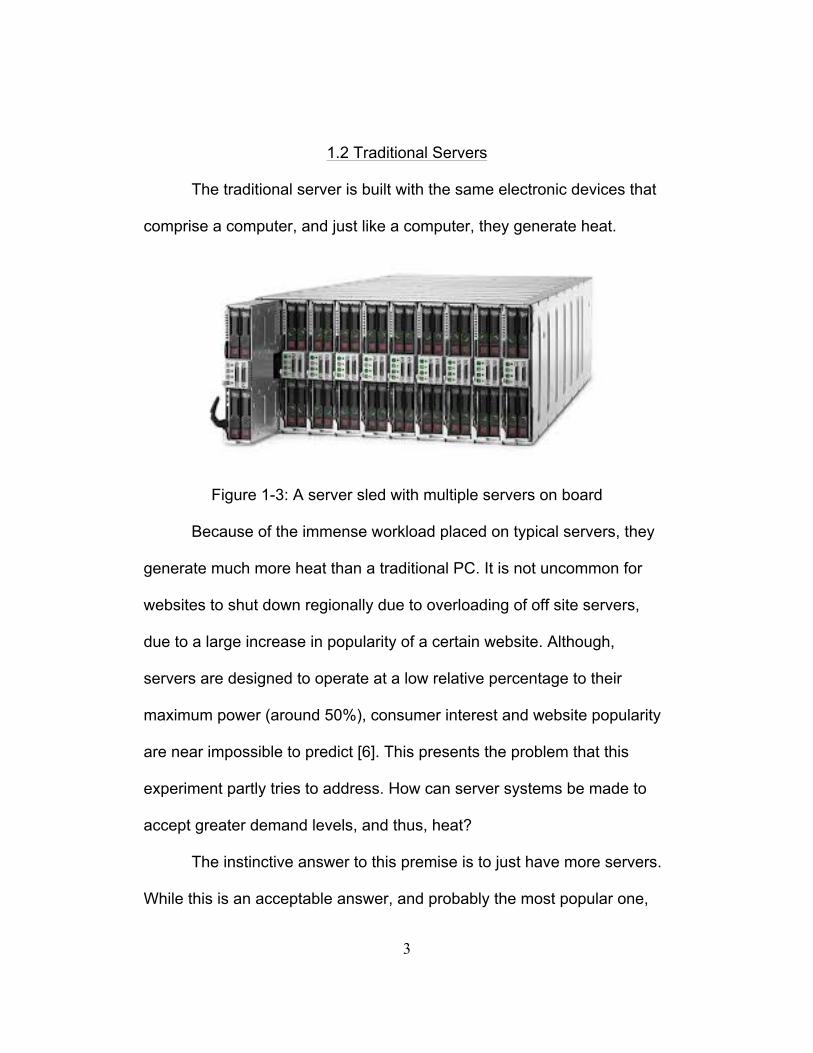
1.2 Traditional Servers

The traditional server is built with the same electronic devices that

comprise a computer, and just like a computer, they generate heat.

Figure 1-3: A server sled with multiple servers on board

Because of the immense workload placed on typical servers, they

generate much more heat than a traditional PC. It is not uncommon for

websites to shut down regionally due to overloading of off site servers,

due to a large increase in popularity of a certain website. Although,

servers are designed to operate at a low relative percentage to their

maximum power (around 50%), consumer interest and website popularity

are near impossible to predict [6]. This presents the problem that this

experiment partly tries to address. How can server systems be made to

accept greater demand levels, and thus, heat?

The instinctive answer to this premise is to just have more servers.

While this is an acceptable answer, and probably the most popular one,

4

companies are realizing that maximizing efficiency of their existing system

produces long term cost savings, significantly impacting the bottom line.

Some examples of increasing the efficiency of the current systems have

included reorganizing the servers within a building to maximize space, or

simply building structures in regions with cooler climates. It is also natural

to assume that the efficiency of the servers themselves have progressed

with time. As microchips have become smaller and more powerful, one of

the largest problems facing the industry is how to cool these systems in

order to maximize their potential.

Traditional servers are air cooled, using forced convection over a

heat sink that is attached to a microchip.

Figure 1-4: Air flow through a traditional server system

5

Fans blow across these heat sinks, and effectively “pull” heat

through the heat sink to the surrounding air. A cooler heat sink increases

the flux (or heat delta) between the microchip and the heat sink, allowing

for faster heat transfer. Over time, these systems have gone from

primitive, to over designed, to peak performance through the use of

experiments just like the one that is about to be discussed.

1.3 Looking Outside of Air-Cooled Systems

As systems have increased in power and heat generation,

companies have begun to look outside the world of air-cooling. The two

most promising alternate cooling methods are water-cooled systems and

oil-cooled systems. Both water and oil are extremely powerful heat

removers, due to their high heat capacities. Water is easy to work with and

cheap to purchase, but it cannot touch the server directly as it is

conductive. Oil on the other hand, is non-conductive and has a higher heat

capacity then water [5]. This allows servers to essentially be immersed in

oil. Oil does have its drawbacks, as it retains dirt and traditional servers

are simply not made to accommodate it.

The experiment that will be discussed in the following pages will

deal with immersion cooling by the use of oil. Although immersion cooling

is very attractive, there are many differences that occur when transitioning

from air to oil cooled systems. These differences must be acknowledged

6

in order to eventually develop a successful design. Because the vast

majority of cooling systems are air driven, the principle differences

between these two methods will be briefly discussed.

7

Chapter 2

Delineation Between Air, Water, and Oil-Cooled Systems

2.1 Compressiblity

While oil and air are still accomplishing the same task in essentially

the same way, the design of an immersion-cooled system may develop

very differently in the future if it gains popularity.

The first difference that must be acknowledged are the properties of

the fluids themselves. Even with no technical understanding of fluid

properties one might postulate that oil is “thicker” or perhaps “stickier” than

water. To dive too deeply into the chemical makeup of each fluid would be

going too far, but we can explore their behaviors. For instance, air is

compressible and oil is considered to be incompressible. That does not

mean that oil could not be compressed slightly under high pressures, or

change volume slightly with large temperature changes, but it does mean

that air can be compressed into a small fraction of its natural pressure at

whatever altitude it resides. Oil simply will not exhibit this behavior [4].

This is relevant to this experiment because air can simply compress in a

system if pressure builds due to pressure drops across certain items,

while oil does not have this ability. This is not necessarily a disadvantage

8

or advantage for either fluid, but it can effect what an efficient design looks

like.

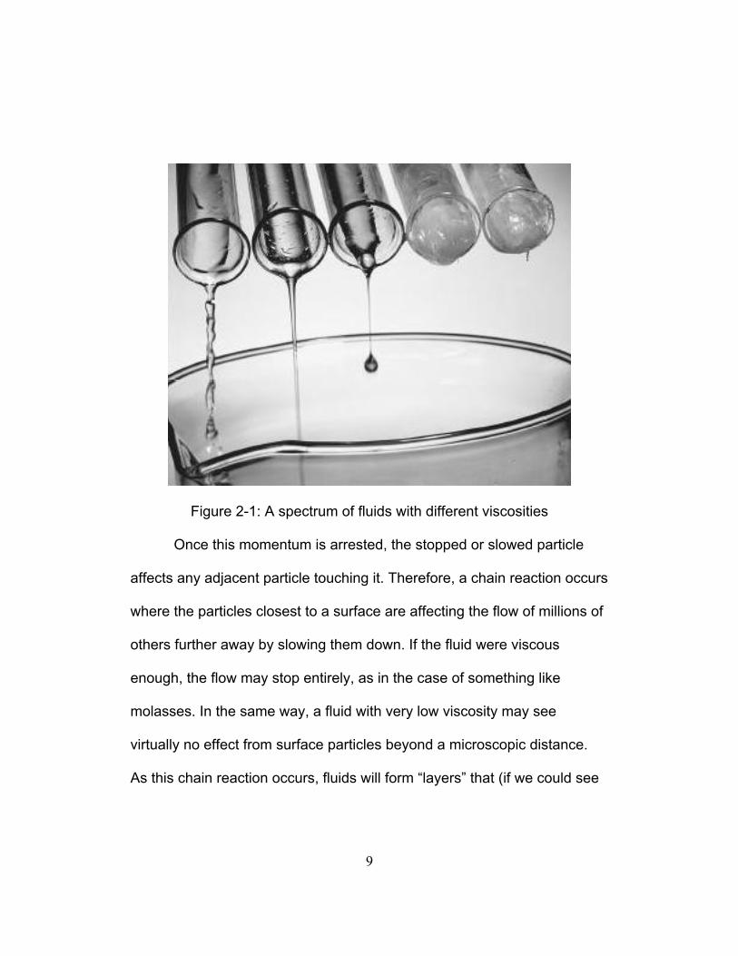
2.2 Viscosity

Another difference in the physical properties of air and oil is

viscosity. This is essentially the “thickness” and “sticky” feeling spoken

about earlier. This, along with density (which is related to viscosity) make

up the most important differences in these fluids with regard to this

experiment. The viscosity of a fluid can be thought of as friction between

the fluid and anything it touches, including itself. As a fluid flows across a

surface, some of the particles in direct contact with the surfaces simply

stop flowing due to the friction between the molecule and the surface.

9

Figure 2-1: A spectrum of fluids with different viscosities

Once this momentum is arrested, the stopped or slowed particle

affects any adjacent particle touching it. Therefore, a chain reaction occurs

where the particles closest to a surface are affecting the flow of millions of

others further away by slowing them down. If the fluid were viscous

enough, the flow may stop entirely, as in the case of something like

molasses. In the same way, a fluid with very low viscosity may see

virtually no effect from surface particles beyond a microscopic distance.

As this chain reaction occurs, fluids will form “layers” that (if we could see

10

them with the naked eye) form waves over a surface. These waves are

called boundary layers.

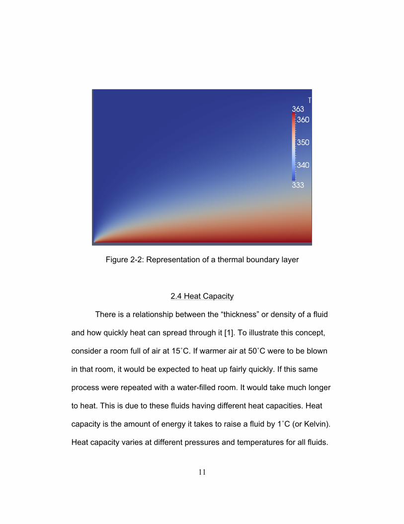
2.3 Boundary Layers

Up to this point, boundary layers have been described as a function

of fluid velocity. Appropriately, these layers are called velocity boundary

layers. Another type of boundary layer exists due to temperature changes

in a fluid. If in the same example given earlier, the bottom surface were

hot, it would be expected that heat would eventually spread through the

container of fluid. If the fluid were static, the heat might spread uniformly

as it rises in the container. However, if flow were present as the heat

moved upward, it would also move along the flow path. This type of

boundary layer is called a thermal boundary layer.

11

Figure 2-2: Representation of a thermal boundary layer

2.4 Heat Capacity

There is a relationship between the “thickness” or density of a fluid

and how quickly heat can spread through it [1]. To illustrate this concept,

consider a room full of air at 15˚C. If warmer air at 50˚C were to be blown

in that room, it would be expected to heat up fairly quickly. If this same

process were repeated with a water-filled room. It would take much longer

to heat. This is due to these fluids having different heat capacities. Heat

capacity is the amount of energy it takes to raise a fluid by 1˚C (or Kelvin).

Heat capacity varies at different pressures and temperatures for all fluids.

12

In all cases, air will have a lower heat capacity than water, and water will

have a lower heat capacity than oil. An example to quantify the difference

in heat capacity in a physical sense is simple to design.

From this example, it is easy to see why immersion cooling is

attractive. Oil could pull vastly more heat away from a system per

molecule than water or air. From this, it is expected that oil could produce

the same cooling effects on a heat sink under lower flow rates, or higher

inlet temperatures, or smaller heat sinks, or under a higher heat output

exerted from the server itself. Each one of these variables were altered in

this experiment to determine if this was indeed a valid expectation. It is

important to note that in the example about heat capacity above, it would

take a proportionally longer time for oil or water to cool down back to room

temperature, as it requires the same amount of energy transaction to cool

off. If a system ever reached the point of overheating with any of these

fluids, the system with oil would by far be in the most danger, as it would

take a great deal of time or energy to cool.

2.5 System Differences

Another difference between oil and air systems is the system itself.

Air cooled systems use fans to pull air from the environment and push it

through a server. Immersion cooled systems need a pump to drive a

circuit. Within this circuit, oil must move through the server to cool it, pass

13

through a pump, and cool through a radiator or heat exchanger. In a large

immersion cooled system, there will most likely be a reservoir of some

type, due to a finite amount of oil. In a system using air, there is a limitless

supply around the system.

14

Chapter 3

Heat Sink Performance

3.1 The Importance of Junction Temperature

To invest more understanding into this topic, and how this specific

experiment relates, it is important to ask how heat sink performance is

measured. Unfortunately, the answer to this question is not quite clear.

The simplest answer is a measurement of how cool a processor will

stay using a certain heat sink. Most processors used in server applications

are designed to record their own temperature in real time [6]. This is also

true of the servers used in this experiment. This method of measurement

heat performance is a baseline measurement, and only measures the one

factor that is ultimately important to the end user. While this method is

effective, it does not assist in understanding the optimum performance of

the heat sink itself. For example, a heat sink that is 40mm tall may keep a

processor at a temperature of 60°C. Under the same loading, it is also

possible to see an 80mm heat keep a processor to nearly the exact same

temperature. The reason that this is possible is because the heat sink is

simply useless at a certain height because eventually the fins of the heat

sink will match the temperature of the environment as you move away

from the processor. From that point upwards, the heat sink is no more

15

than a hunk of metal taking up space. While processor temperatures are

good to monitor and useful data, it is important as an engineer to look for

superior ways to measure heat sink performance. One important thing to

note about processor temperature is that variables must be maintained in

order to establish some type of relativity within the experiment. If variables

are randomly selected, and the processor temperature is recorded

randomly, then no good data comes from the experiment. The data would

only show that a processor maintained better temperatures under certain

random circumstances. If single variables are changed, combined, and

repeated to form a matrix, then curves can be drawn to establish when the

heat sink begins to peak in its performance. This was the method that was

undertaken in this experiment. However, much more than just processor

temperature was gathered from the test.

3.2 Thermal Resistance

One way to measure heat sink performance is to measure the

overall thermal resistance of the heat sink. This allows for the heat sink to

be viewed as a single piece, instead of looking at individual fins or pins [5].

In industry, this is the principle barometer of performance of heat sinks in

air-cooled systems. When shopping for a heat sink, one would ultimately

find technical information that included a graph that showed both the

16

thermal resistance and pressure drop at different flow rates. One such

example is shown below in Figure 3-1.

Figure 3-1: Cooling performance measurement of the tested 2U heat in

air-cooling [6]

It is important that air-cooled systems were mentioned alone when

discussing these graphs. This is simply because the vast majority of heat

sink thermal resistance is not measured in an immersion cooled systems.

To important points should be gleaned from this. First, this means that this

test is measuring something that has not yet been measured in this

system. Secondly, it is very reasonable to assume that the heat sinks

used in this experiment were strictly designed for air-cooling, and thus

Pres

sure

Dro

p (k

g/cm

2 )

17

may encounter natural hurdles to achieving optimum performance in an

immersion-cooled system.

Thermal resistance of a heat sink can be characterized in the

following equation.

𝜃!" = 𝑇!"#$%&'# − 𝑇!"#$%&'

𝛲

Simply put, thermal resistant is the amount that a given object

resists heat traveling through it [4]. A high heat resistance would be very

undesirable for any heat sink, as its job is to transmit heat from the

processor to the surrounding environment.

3.3 Fin Efficiency and Boundary Layers

There are some parameters that are calculable, but ultimately will

not be utilized in this experiment’s scope. One of these parameters is fin

efficiency. Fin efficiency is the usage of the fin to distribute heat to

environment. Earlier, an idea was discussed that only part of a heat sink’s

height may be used to move heat to the environment. The rest of the

length of the fins would be useless, and therefore, inefficient. Fin efficiency

can be calculated by using the following equation by employing the

thermal efficiency above.

𝜂!"! =1 − 𝜃!"𝐴!"#$ℎ𝜃!"𝑁!"#𝐴!"#ℎ

18

In this equation, Abase is the area of the base of the heat sink, NFIN is the

number of fins on the heat sink, AFIN is the area of one side of one fin on a

heat sink, and h is the convection coefficient [3].

Boundary layers are also parameters that can be calculated. For

this experiment we will not investigate this. Most boundary layer equations

rely on strict geometry. Due to this test occurring in a server, the oil will be

passing against uneven terrain, with significant protrusion and geometry

variations. To calculate the exact layer structure would be largely a waste

of time, and does not help us to define the overall performance of the heat

sink itself. Perhaps the boundary layers moving through the heat sink

would be useful to explore, but not in this experiment.

19

Chapter 4

Experimental Characterization of the Current System

4.1 Modifying the Existing Server

A large part of this thesis work was to set up an experiment to test

heat sinks inside of an actual server for immersion cooling. This task

proved to be quite challenging and even slightly expensive. This server

was not designed to accommodate just this single experiment, but a whole

host of future experiments to build off of this one.

The first challenge faced when creating this apparatus was to

“unbuild” the current server system. The original server consisted of a

torpedo-like aluminum case with twin fans on one end designed to blow air

across two heat sinks. These two heat sinks were placed in series, not

side-by-side.

Figure 4-1: A front view of the tested server system without the lid

20

Figure 4-2: A top view of the air-cooled server before cutting

This proved to be an interesting design, because it would ultimately

lead to one heat sink having a different inlet temperature than the other.

Another interesting design in the current server was the lid. Each server is

self-contained and directs the flow of air over the heat sink by using a lid

that forces the air over the heat sinks. Because this lid was unique only to

the baseline heat sink, it could not be used for this experiment to provide

an “apples to apples” relationship in the flow direction between heat sink

sizes. As heat sinks would be dropped to lower and lower heights, the

space between the ceiling and the top of the heat sinks would increase,

allowing for more and more ineffective flow bypass. The solution to this

will be discussed in a few moments, but it was clear that the currently lid

would need to be scrapped.

21

Figure 4-3: A view of the ducting on the lid of the server to control airflow

The next things that had to be removed were the fans. In immersion

cooling (as stated early), pumps are used in lieu of fans, and therefore

they would just be creating pressure drop unnecessarily. Part of the

overall length of the server was portioned to hold the fans, and allow for

air flow to fully develop as it passed the heat sinks. Both ends of the

server bend inward for structural support. This was unnecessary for the

purpose of this test, and would contribute to more pressure drop across

the system. It was decided after some consideration to cut off the two

22

ends of the server in order to make the pathway for the oil as unobstructed

as possible.

4.2 Server Container Design

Originally, the server was never meant to hold liquid, and certainly

could not now with multiple holes already existing throughout its interior

and open ends. Therefore, a clear acrylic case was made to house the

server. The case was sized so that only the width of the server would fit

into it. A small amount of extra room was created for wire routing and

handling purposes, but those gaps were filled with more acrylic as the

server was placed inside the case. Two holes were dilled and tapped on

each end of the case to fit a ½” nominal thread pattern thread in order to

serve as inlets and outlets to the server. The inlet and outlet ports were

placed low in the tank, because the fluid level would be changing as the

height of the heat sink changed.

23

Figure 4-4: The acrylic case housing the server with the lid raised

Now that the case was constructed and the server was properly fit

inside, the ceiling had to addressed. In the original server, the ceiling

piece not only directed flow downward, but did not allow for air to travel

around the sides of the heat sink as well. This was perhaps the greatest

challenge for this experiment. If multiple heat sinks were to be used, then

multiple channeling ducts would need to be created for each heat sink set.

This effort was distressing and led to very expensive or time-consuming

ideas. After much consideration, hard foam and an acrylic sheet appeared

to be the best answer. The foam would be cut to straddle the DIMs that

24

were lined up long the sides of the heat sinks, and protrude outward

toward the heat sinks to within a few millimeters of the sides.

Figure 4-5: A view of the foam cut to force flow through the heat sinks.

The lid is also currently placed on the foam in this figure, although it is

difficult to see.

These foam pieces would also have to be cut to the height of

whatever heat sink was being currently used. In addition, a sheet of acrylic

was cut to lie just with the thickness of the server and lay directly on the

foam, almost touching the tops of the heat sinks. As the heat sinks were

lowered in height, the foam would be cut down to match it. One hazard

that was originally feared were tiny pieces of foam being sent adrift in the

oil and possibly clogging the flow meter or damaging the pumps or the

25

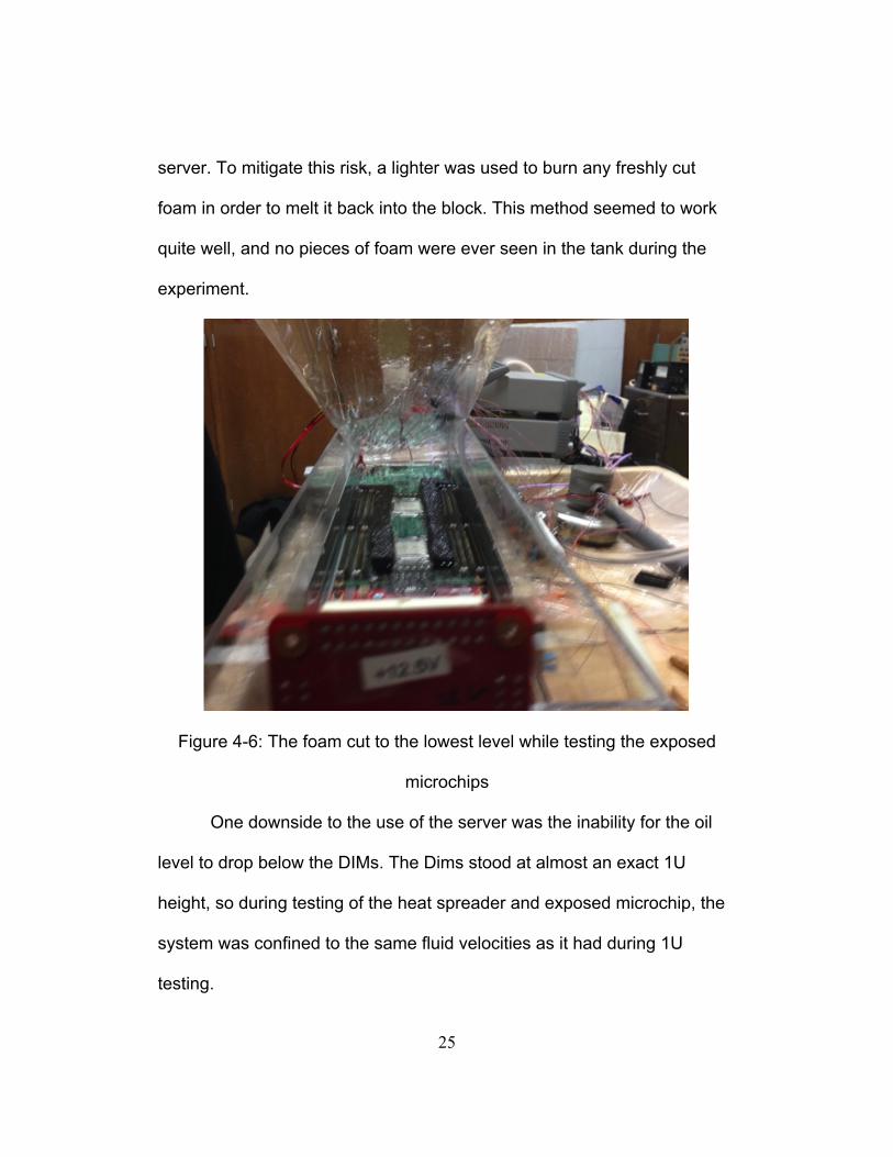
server. To mitigate this risk, a lighter was used to burn any freshly cut

foam in order to melt it back into the block. This method seemed to work

quite well, and no pieces of foam were ever seen in the tank during the

experiment.

Figure 4-6: The foam cut to the lowest level while testing the exposed

microchips

One downside to the use of the server was the inability for the oil

level to drop below the DIMs. The Dims stood at almost an exact 1U

height, so during testing of the heat spreader and exposed microchip, the

system was confined to the same fluid velocities as it had during 1U

testing.

26

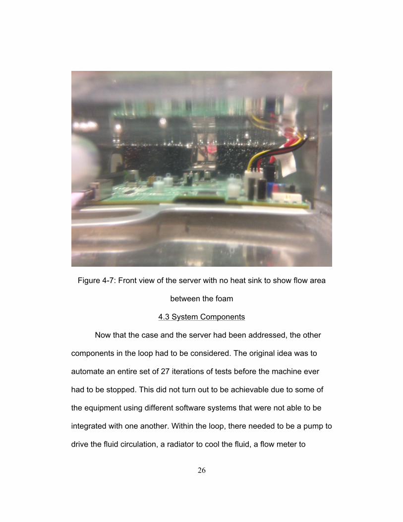
Figure 4-7: Front view of the server with no heat sink to show flow area

between the foam

4.3 System Components

Now that the case and the server had been addressed, the other

components in the loop had to be considered. The original idea was to

automate an entire set of 27 iterations of tests before the machine ever

had to be stopped. This did not turn out to be achievable due to some of

the equipment using different software systems that were not able to be

integrated with one another. Within the loop, there needed to be a pump to

drive the fluid circulation, a radiator to cool the fluid, a flow meter to

27

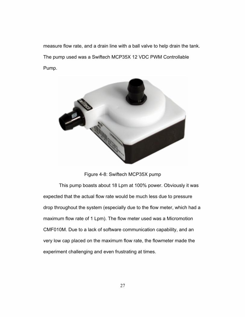
measure flow rate, and a drain line with a ball valve to help drain the tank.

The pump used was a Swiftech MCP35X 12 VDC PWM Controllable

Pump.

Figure 4-8: Swiftech MCP35X pump

This pump boasts about 18 Lpm at 100% power. Obviously it was

expected that the actual flow rate would be much less due to pressure

drop throughout the system (especially due to the flow meter, which had a

maximum flow rate of 1 Lpm). The flow meter used was a Micromotion

CMF010M. Due to a lack of software communication capability, and an

very low cap placed on the maximum flow rate, the flowmeter made the

experiment challenging and even frustrating at times.

28

Figure 4-9: Flowmeter used in the experiment

The radiator used was a Swiftech MCR220QP. The radiator was

initially thought to possibly not have enough power to cool the oil, due to

the oils high heat capacity. However, due to the relatively low flow rates

achieved, the oil had plenty of time to cool while passing through the

radiator. In fact, the radiators had to be blocked with poster board during

experiments that were designed to have a hotter inlet temperature,

because the radiator running at idle was cooling the oil down below the

desired temperature.

29

Figure 4-10: Radiator used in the experiment

All of these components were interconnected using clear tubing in

the circuit configuration shown below.

Figure 4-11: A general flow path of the oil during the experiment

30

Figure 4-12: A top view of the actual experimental flow path

4.4 Control System Integration

The first challenge of the technical side of this set up was

understand how to gather the proper data, and use data in control

systems to at least partially automate the system. The most important data

was of course temperature data. Temperature readings were desired at

the inlet of the server, right in front and behind each heat sink, and the

temperature of the chip itself. The temperature of the chips was given by

the server through the use of the server software. Although this software

could not be integrated with Labview software used in the Data Acquisition

Units, it could be given the same set of time stamps by using scripts in the

31

programming. This allowed for very accurate measurements of each core

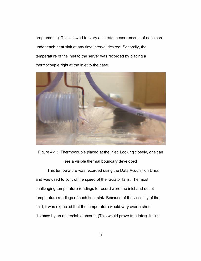
under each heat sink at any time interval desired. Secondly, the

temperature of the inlet to the server was recorded by placing a

thermocouple right at the inlet to the case.

Figure 4-13: Thermocouple placed at the inlet. Looking closely, one can

see a visible thermal boundary developed

This temperature was recorded using the Data Acquisition Units

and was used to control the speed of the radiator fans. The most

challenging temperature readings to record were the inlet and outlet

temperature readings of each heat sink. Because of the viscosity of the

fluid, it was expected that the temperature would vary over a short

distance by an appreciable amount (This would prove true later). In air-

32

cooled servers, thermal mixing of the air occurs at a much greater speed

than in oil, which develops more pronounced thermal boundary layers.

Thus, in a traditional server only one or two temperature readings would

be necessary to take in order to get an accurate temperature reading of

the inlet and outlet. It was concluded that for oil, six thermocouples should

be placed in two rows and three columns in front and behind of heat sink.

All in all, dozens of thermocouples were created to achieve the desired

pattern of sensors. These readings would help calculate the average

thermal resistance of each heat sink.

Figure 4-14: A set of 6 thermocouples measuring temperature between

the heat sinks.

33

Figure 4-15: A closer view of two thermo couples in the fluid

Having thermal resistance would help compare oil-cooled heat

sinks to the traditional air-cooled systems. In order to control the fan

speed, an Arduino Mega 2560 control board was utilize to communicate

the control function between the computer and the fans in order to

maintain a precise inlet temperature reading throughout each iteration.

34

Figure 4-16: The Adriano control board used to control the fans

4.5 Software Integration

Although a great deal of time and energy was spent on the building

of the experimental apparatus, the software was another issue entirely.

Two data acquisition units and four power supplies were necessary for this

effort.

35

Figure 4-17: A stack of power supplies and data acquisition units

Three different software systems were also used in this effort. The

server software was able to run alongside of the LabView software, but

the flow meter software was not able to work appreciably to control the

pumps. Because of this, the pumps were manually controlled between

every three iterations of the experiment.

36

Figure 4-18: Three fans placed in series on the outlet side of the

apparatus. Fan sinks are seen attached using rubber bands to prevent

overheating.

37

The flow meter software was able to record the density, viscosity,

volumetric flow rate, and mass flow rate of the system into a folder.

Figure 4-19: A screenshot of the flow meter software

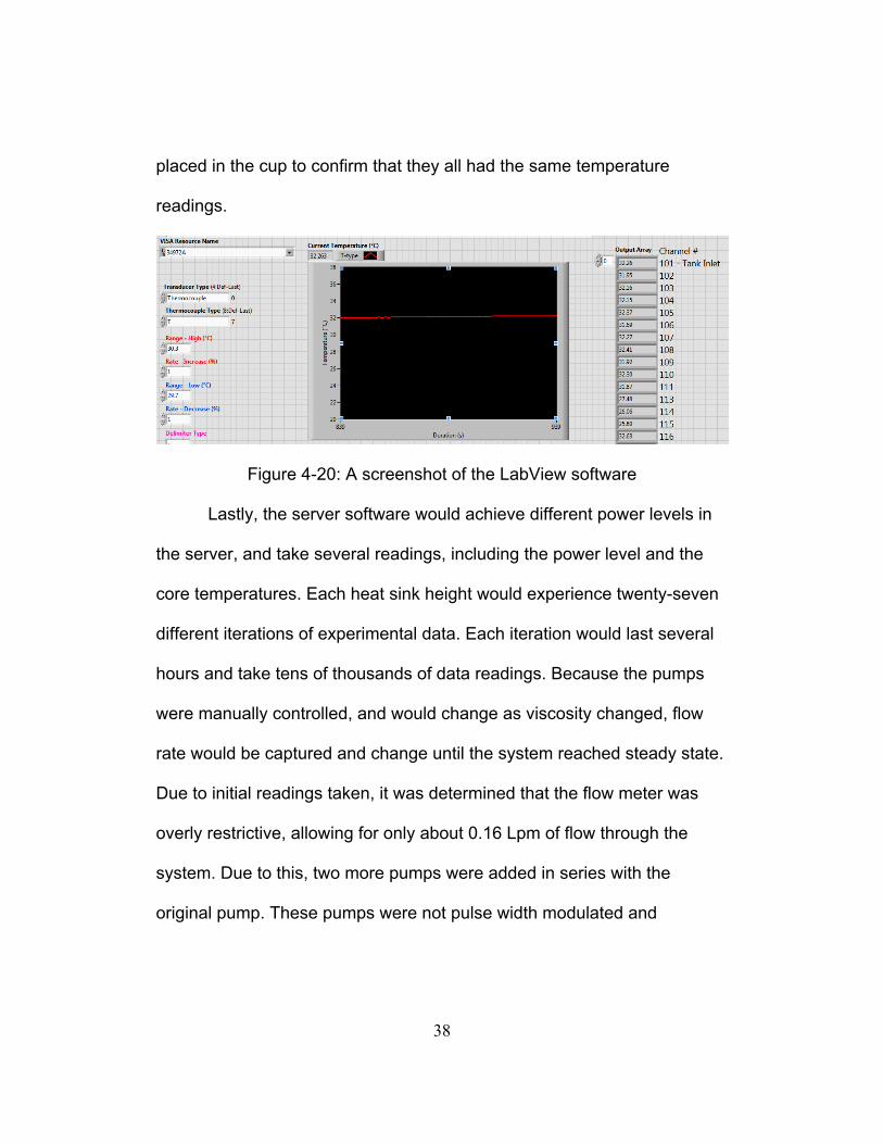
The LabView software would take all the thermocouple readings,

and control the radiator fans in order to control the inlet temperature. In

order to get accurate measurements from the LabView software, it was

imperative to insure that the readings taken by the thermocouples were

uniform throughout the experiment. If a thermocouplebroke, a large

negative reading would commence. This would throw off any averages

later in the data reduction portion of the test. To test these thermocoples,

a large cup of ice water was purchased, and all thermocouples were

38

placed in the cup to confirm that they all had the same temperature

readings.

Figure 4-20: A screenshot of the LabView software

Lastly, the server software would achieve different power levels in

the server, and take several readings, including the power level and the

core temperatures. Each heat sink height would experience twenty-seven

different iterations of experimental data. Each iteration would last several

hours and take tens of thousands of data readings. Because the pumps

were manually controlled, and would change as viscosity changed, flow

rate would be captured and change until the system reached steady state.

Due to initial readings taken, it was determined that the flow meter was

overly restrictive, allowing for only about 0.16 Lpm of flow through the

system. Due to this, two more pumps were added in series with the

original pump. These pumps were not pulse width modulated and

39

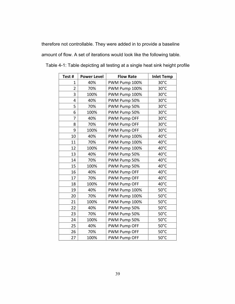
therefore not controllable. They were added in to provide a baseline

amount of flow. A set of iterations would look like the following table.

Table 4-1: Table depicting all testing at a single heat sink height profile

Test # Power Level Flow Rate Inlet Temp 1 40% PWM Pump 100% 30°C 2 70% PWM Pump 100% 30°C 3 100% PWM Pump 100% 30°C 4 40% PWM Pump 50% 30°C 5 70% PWM Pump 50% 30°C 6 100% PWM Pump 50% 30°C 7 40% PWM Pump OFF 30°C 8 70% PWM Pump OFF 30°C 9 100% PWM Pump OFF 30°C 10 40% PWM Pump 100% 40°C 11 70% PWM Pump 100% 40°C 12 100% PWM Pump 100% 40°C 13 40% PWM Pump 50% 40°C 14 70% PWM Pump 50% 40°C 15 100% PWM Pump 50% 40°C 16 40% PWM Pump OFF 40°C 17 70% PWM Pump OFF 40°C 18 100% PWM Pump OFF 40°C 19 40% PWM Pump 100% 50°C 20 70% PWM Pump 100% 50°C 21 100% PWM Pump 100% 50°C 22 40% PWM Pump 50% 50°C 23 70% PWM Pump 50% 50°C 24 100% PWM Pump 50% 50°C 25 40% PWM Pump OFF 50°C 26 70% PWM Pump OFF 50°C 27 100% PWM Pump OFF 50°C

40

Between every pump power level change, an operator would be

accountable for restarting the data collection process, inspecting the tank,

and switching the pump power level manually. Although this process

proved tedious, it allowed for regular checking of the system to ensure all

sensors were in the correct locations.

4.6 Early Challenges

During the initial stages of development of experimental

setup, several problems were encountered and overcome or negotiated.

First, tank leaked on two separate occasions, leading to the tank needing

to be drained and mended. Next, the PWM pump that was used for former

tests would not function properly. It could not be expected to provide

accurate power levels during testing, so a new one had to be ordered.

Also, as discussed previously, the flow meter software was incapable of

communicating with the Labview software, making flow control impossible.

Throughout the experiment, thermocouples would often break when being

moved and would need repairs. In the end, each one of these obstacles

was overcome either by negotiating to a different data gathering tactic, or

finding/buying a replacement part.

41

Chapter 5

Experimental Expectations

5.1 Laminar Flow

Before the experiment began, several expectations were already in

place from a theoretical understanding of heat transfer and fluid dynamics.

First, it was expected that only laminar flow would be encountered during

this experiment. Laminar flow is dependent on the Reynolds number,

which can be determined by dividing the inertial forces of a fluid over the

viscous forces. Below is a table of the dynamic viscosity of air, water, and

oil at the temperature ranges used in this experiment [1].

Table 5-1: Property comparisons between air, oil, and water

Heat Capacity

(kJ/kgK) K (W/mK)

Kinematic Viscosity

(mm^2/s)

Air 1.01 0.02 .016

Oil 1.67 0.13 16.02

Water 4.19 0.58 0.66

It is clear to see that oil has viscosities that are orders of

magnitudes higher than air or water. When calculating the Reynolds

number equation, it is plain to see that a high viscosity will result in in a

42

lower Reynolds number. This simply means that oil is much more unlikely

to exhibit turbulence than air at a given velocity. Due to an already low

projected flow rate in this experiment (because of a 1 Lpm flow cap on the

flow meter), it was hypothesized that no turbulence would occur during

this test.

5.2 Thermal Data Variance

This theoretical understanding provided further insight into what

would occur with the boundary layers. Boundary layers are dependent on

the Reynolds number of flow to determine their width at a given distance.

A low Reynolds number would give a larger boundary layer that would not

reach turbulence. Turbulence is the principle cause of thermal mixing,

which would allow for an average temperature reading to be taken from

one location near the heat sink. Due to large, pronounced boundary

layers, it was again assumed that we would see relatively large

temperature variations at different heights even at the inlet to the first heat

sink.

Furthermore, it was expected that the thermal resistance of a heat

sink should remain constant throughout the experiment at a given inlet

temperature. As stated before, thermal resistance is dependent on inlet

temperature, junction temperature, and power being dissipated. This

means that thermal resistance is not a function of flow rate (and

43

subsequently flow velocity). These parameters should help identify

performance levels of the heat sinks as the experiment continues.

5.3 Thermal Data Considerations

Another goal of this test was to be able to create comparable data

between each variable that could be graphically represented. Once it was

discovered that the pumps could not be controlled as a function of the PID

controller in LabView, it became clear that flow rates would not be able to

be matched perfectly between iterations, especially at different inlet

temperatures. Luckily, flow rates are the independent variable in most

performance graphs in air-cooled systems. This means that it is not

necessary to match flow rates across different iterations, and performance

between different experimental iterations can still be graphically

represented in a comparable form. Although the flow rates will not achieve

the same values from iteration to iteration, enough data points will be

captured to create a curve. This curve will then be plotted across the

range of all of the flow rates captured in order to compare them. While

flow rate can remain independent, it is imperative that the power levels,

inlet temperatures, and heights of the heat sinks are carefully controlled.

44

Chapter 6

Physical Observations

6.1 Visible Boundary Layers

Early observations of the experiment were intriguing. Before the

technical data was analyzed, certain characteristics were observed and

noted within the experiment. These observations were later used in

concert with the digitally gathered data to explain possible reasons for

these observations.

First, one immediate difference to air-cooled servers was a

physically viewable thermal boundary layer coming into the server through

the inlet valve. It was not expected that anything would be seen, but at all

times a strong layer of fluid could be seen until it reached the front of the

server. It should also be noted that at one point, it was decided to run the

test without heat sinks at all. During this quick experiment, the microchips

became dangerously hot, but did maintain temperatures between 85-

100°C. During this time period, very visible thermal layers could be seen

leaving the chip surface.

45

Figure 6-1: Thermal boundary layers visibly seen on the processor chip

Unusually, the visible fluid flow leaving the inlet would not always

behave consistently throughout the experiment. Even while using the

same set of heat sinks, often the flow path would immediately deviate

toward the right side of the server upon leaving the inlet. It was

conjectured that the tank may have not been level, but the fluid flow path

would change without the tank ever moving. The cause for this sudden

change in flow path was never determined.

46

Chapter 7

Experimental Data Results

7.1 Constraining Data Time Periods

As explained earlier, the first iterations of the test were automated

only through the three desired power levels of the server. To be

conservative, each of these automated stages were given 12 hours to

complete, which would allow 4 hours for the completion of each power

level. After the three sets of data were completed (taking approximately 36

hours), the first set of raw data was placed into Excel to get an idea of

when steady state was reached. It was important to accomplish this task

as early in the process as possible in order to make sure steady state was

being achieved, and to decide on a more efficient time frame to run each

power level. When the first set of core temperatures were placed against

time graphically, the three power levels were clearly seen in the graph

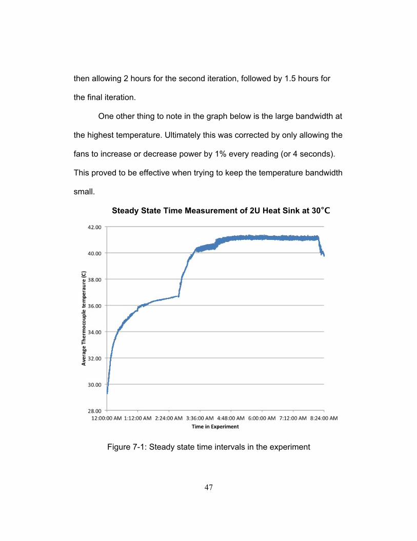
(Figure 7-1). The first temperature increase took a long time to reach

steady state, because it was coming from room temperature. The

subsequent temperature change reached steady state very quickly. After

analyzing multiple cases, it was determined that appropriate data could be

gathered in about 6 hours by shortening the first iteration to 2.5 hours, and

47

then allowing 2 hours for the second iteration, followed by 1.5 hours for

the final iteration.

One other thing to note in the graph below is the large bandwidth at

the highest temperature. Ultimately this was corrected by only allowing the

fans to increase or decrease power by 1% every reading (or 4 seconds).

This proved to be effective when trying to keep the temperature bandwidth

small.

Steady State Time Measurement of 2U Heat Sink at 30°C

Figure 7-1: Steady state time intervals in the experiment

48

7.2 Comparing inlet and outlet temperatures of the heat sinks

The next set of desired data was the tempoerature readings of the

inlet and outlet temperatures of the heat sinks themselves. As discussed

earlier, each heat sink had 6 thermocouples even spaced in front and

behind it. First, it was desired to compare the thermal differences between

thermocouples, both from side to side and top to bottom. Also, it was

important to explore if the delta between thermocouples was consistent at

all three locations.

Figure 7-2: Average difference in temperature within the three

thermocouple groupings

0.00

2.00

4.00

6.00

8.00

10.00

12.00

0% 20% 40% 60% 80% 100% 120% Largest T

empe

rature Differen

ce Between

Thermocou

ples (°C)

Server Power Percentage (%)

Thermocouple Groups Average ΔT Between Min and Max Temperatures

Inlet to Heat Sink 1

Outlet to Heat Sink 1


49

Ultimately, it was determined that the Inlet to the first heat sink had the

smallest temperature difference between the maximum and minimum

thermocouple reading.

Figure 7-3: Average difference in temperature between thermo couple

groupings

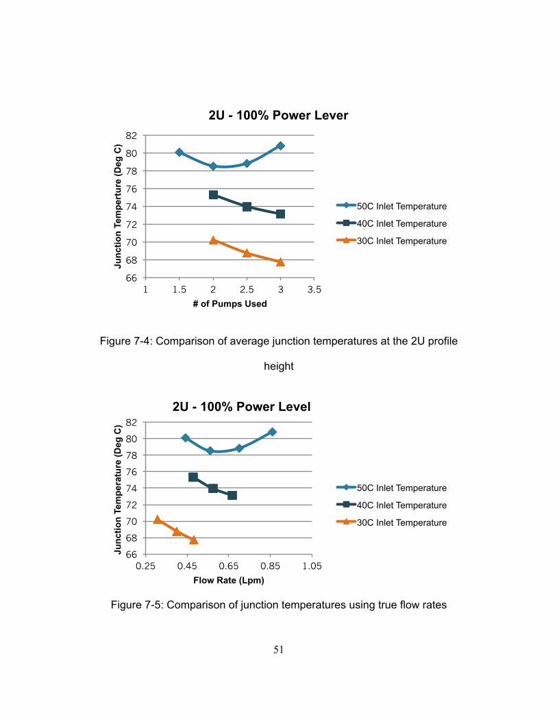
7.3: Performance characteristics of a 2U heat sink at different flow rates

At this time it was necessary to get into the meat of the results. It

took several days to take the hundreds of thousands of data points and

reduce them into usable information. First the different software system

35

37

39

41

43

45

47

49

51

53

0% 20% 40% 60% 80% 100% 120% Thermocou

ple Group

average Tem

perature (°C)

Server Power Level (%)

Temperature Difference Between Thermocouple Groups

Inlet to Heat Sink 1



50

recordings had to be compiled into different spreadsheets and then

melded into master templates. Some initial issues with this procedure

involved data scripts importing time stamps as different time zones, so

one of the programs had to have its time entries changed by one hour to

match its counterparts. Once all data was transferred into a master

template, a master-master template needed to be created to compare the

different height heat sink performances against one another. Before

comparing heat sinks to one another, it was necessary to find the best

performance level that the 2U heat sink could achieve. At first the pumping

power levels were used as the independent variable, but the actual flow

rate proved to be more reliable and valuable for future experiments.

51

Figure 7-4: Comparison of average junction temperatures at the 2U profile

height

Figure 7-5: Comparison of junction temperatures using true flow rates

66

68

70

72

74

76

78

80

82

1 1.5 2 2.5 3 3.5

Junc

tion

Tem

pert

ure

(Deg

C)

# of Pumps Used

2U - 100% Power Lever

50C Inlet Temperature



66

68

70

72

74

76

78

80

82

0.25 0.45 0.65 0.85 1.05

Junc

tion

Tem

pera

ture

(Deg

C)

Flow Rate (Lpm)

2U - 100% Power Level




52

Figure 7-6: Comparison of thermal resistances between flow rates

Figure 7-7: Junction temperatures at 70% power levels

0.250

0.270

0.290

0.310

0.330

0.350

0.370

0.390

0.2 0.4 0.6 0.8

Ther

nmal

Res

ista

nce

(K/W

)

Flow Rate (Lpm)

2U - 100% Power Level




70

72

74

76

78

80

82

84

86

0.2 0.4 0.6 0.8 1

Junc

tion

Tem

pera

ture

(Deg

C)

Flow Rate (Lpm)

2U - 70% Power




53

Figure 7-8: Thermal resistances at 70% power levels

Figure 7-9: Junction temperatures at 40% power levels

0.25

0.27

0.29

0.31

0.33

0.35

0.37

0.39

0.41

0.43

0 0.2 0.4 0.6 0.8 1

Ther

mal

Res

ista

nce

(K/W

)

Flow Rate (Lpm)

2U - 70% Power




50

55

60

65

70

75

0.25 0.45 0.65 0.85 1.05

Junc

tion

Tem

pera

ture

(Deg

C)

Flow Rate (Lpm)

2U - 40% Power




54

Figure 7-10: Thermal resistances at 40% power levels

7.3: Comparison of heat sinks at different profile heights

It was easily determined from this data that the 30 degree inlet

temperature provided the best performance of the 2U heat sink. With this

information, it was decided to test the other profiles at the same inlet

temperature and compare their performances. The results that follow

show the data obtained for junction temperature and thermal resistance of

the heat sinks. It should be noted that the spreader data could only be

obtained at the highest flow rate, because a lower flow rate would cause

the server to overheat.

0.25

0.27

0.29

0.31

0.33

0.35

0.37

0.39

0.41

0 0.2 0.4 0.6 0.8 1

Ther

mal

Res

ista

nce

(K/W

)

Flow Rate (Lpm)

2U - 40% Power




55

Figure 7-11: Heat sink junction temperature comparison at 100% server power

Figure 7-12: Heat sink thermal resistance comparison at 100% server power

60

65

70

75

80

85

90

95

100

0.28 0.33 0.38 0.43 0.48 0.53 0.58

Junc

tion

Tem

pera

ture

(Deg

C)

Flow Rate (Lpm)

Heat Sink Comparison - 100% at 30ºC

2U

1U

SPREADER

0.3

0.35

0.4

0.45

0.5

0.55

0.6

0.65

0.25 0.35 0.45 0.55 0.65

Ther

mal

Res

ista

nce

(K/W

)

Flow Rate (Lpm)


Series1

Series2

Series3

56


power


power

60

65

70

75

80

85

90

95

100

0.28 0.33 0.38 0.43 0.48 0.53 0.58

Junc

tion

Tem

pera

ture

(Deg

C)

Flow Rate (Lpm)


2U

1U

SPREADER

0.3

0.35

0.4

0.45

0.5

0.55

0.6

0.65

0.3 0.35 0.4 0.45 0.5 0.55

Ther

mal

Res

ista

nce

(K/W

)

Flow Rate (Lpm)


2U

1U

SPREADER

57

Figure 7-15: Heat sink junction temperature comparison at 40% power

Figure 7-16: Heat sink thermal resistance comparison at 40% power

50

55

60

65

70

75

80

85

90

0.2 0.3 0.4 0.5 0.6

Junc

tion

Tem

pera

ture

(Deg

C)

Flow Rate (Lpm)


2U

1U

Spreader

0.3

0.35

0.4

0.45

0.5

0.55

0.6

0.65

0.28 0.33 0.38 0.43 0.48 0.53

Junc

tion

Tem

pera

ture

(K/W

)

Flow Rate (Lpm)


2U

1U

SPREADER

58

Chapter 8

Conclusion

8.1 Conclusions

From this data, we can conclude many things. However, the

principle purpose of this experiment was to determine whether the heat

sink profile can be lowered to the height of 1U, which was the same height

as the DIMMs. The results unquestionably show that this is possible, even

if the server is operating at 100% power at very low flow rates. At higher

flow rates, we could assume that a spreader may even be sufficient. To

cool the server.

Figure 8-1: Suggested new profile height for heat sink

59

From this experiment it was also determined that strong boundary

layers exist in immersion cooled systems, and that viscosity has a large

affect on cooling capability and should be a major driver for heat sink

design. If a flow loop were designed for oil, it should be as simple as

possible, mitigating as much pressure drop in the system as possible.

When comparing the system to air, it is difficult to make a direct

comparison. Ultimately, the entire system will have to be taken into

account, not just the heat sinks. When companies ultimately decide

whether immersion-cooled systems are cost prohibitive or not, they must

measure the entire system by cost and performance. More studies will

ultimately have to be performed to analyze each aspect of the system.

8.2 Recommendations

Although a great deal of data and information was taken from this

experiment, further experimentation could be quite useful. The first

recommendation to improve results is to acquire a flowmeter with higher

flowrate capability. The fact that the flowmeter would not allow the system

to achieve flowrates of even 1m/s hindered the bandwidth of results. Much

more clarity could have been achieved with higher flow rates. The

bandwidth was so small from flow rate to flow rate that results did not have

much room to vary. If a range up to 5 m/s were achievable, much more

60

data could be gathered, and true performance curves could be found,

showing where heat sinks stop appreciable performance.

Another recommendation would be to use pin fin heat sinks, and

heat sinks with larger gaps between fins. This would account for the

viscosity of oil. The heat sinks used were designed for air, which has a

much lower viscosity. Having more space between fins would help lower

pressure drop across the heat sink.

A last recommendation would be to use servers in a vertical

position, and see if performance improves as natural convection is utilized.

It was postulated from the experiment and through visibly watching

boundary layers that oil moves with purpose across boundary layers due

to natural convection.

61

References

1. Theodore L. Bergman, Adrienne S. Lavine, Frank P. Incropera,

David P. Dewitt (2011) Fundamentals of Heat And Mass Transfer.

New Jersey: John Wiley & Sons

2. Lee Seri (2010) Optimum Design And Selection Of Heat Sinks.

New Hampshire: Springer

3. P. Teertstra, M.M. Yovanovich, J.R. Culham (2010) Analytical

Forced Convection Modeling of Plate Fin Heat Sinks. Waterloo,

Canada

4. Robert E. Simons (2003) Estimating Parallel Plate-Fin Heat Sink

Thermal Resistance. New York.

5. Joshi Y, Kumar P (2012) Energy Efficient Thermal Management of

Data Centers. New York: Springer

6. http://www.datacenterknowledge.com/archives/2011/04/07/closer-

lookfacebooks-new-open-compute-servers

62

Biographical Information

Trevor McWilliams is originally from the Dallas-Ft. Worth area. He

currently works at Lockheed Martin Missile and Fire Control in Grand

Prarie, Texas, as mechanical engineer in the leadership development

program. Before fromal education, he served four years in the United

States Army as a paratrooper, serving tours in Iraq and Afghanistan.

thesis in template - university of texas at arlington

Documents