thesis final march

A Study on Mean-shift based Object Tracking

i

The undersigned have examined the thesis entitled ‘A STUDY ON MEAN-SHIFT

BASED OBJECT TRACKING’ presented by Nguyen Duy Trung Duong, Ho Hai

Nam, Le Hong Thang and hereby certify that it is worthy of acceptance.

Date Advisors name


ii

ABSTRACT

An efficient method for tracking of non-rigid objects in a video is proposed. The central computational module is based on the mean-shift iterations and finds the most probable target position in the current frame. The dissimilarity between the target model (its color distribution) and the target candidate is expressed by a metric derived from the Bhattacharyya coefficient. The capability of the tracker to handle in partial occlusions, significant clutter, and target scale variations, is demonstrated for several image sequences.

The implementation of the kernel-based tracking of moving video objects based on the mean shift algorithm is also presented. We show that the algorithm performs exceptionally well on moving objects in many videos and that it is robust to changes in shape as well as partial occlusion. We also propose possible extensions of the current implementation and future work that might be done in this area.


iii

ACKNOWLEDGEMENT

This diploma thesis was written in the year 2014. We would like to take this opportunity to express our gratitude and sincere thanks to our respected supervisor Dr. Ho Phuoc Tien from Electronic and Telecommunication Engineering Department, Da Nang University of Technology for his invaluable guidance, insight, and support he has provided throughout the course of this work. We also would like to thank all faculty member and staff of the Center of Excellence for their extreme help throughout the course.

An assemblage of this nature could never have been attempted without reference to and inspiration from the works of others whose details are mentioned in the reference section. We acknowledge our indebtedness to all of them.

Last but not the least our sincere thanks to all our friends, who have patiently extended all sorts of help for accomplishing this undertaking.

Danang, March 2014

Nguyen Duy Trung Duong

Ho Hai Nam

Le Hong Thang


iv

TABLE OF CONTENTS

ABSTRACT ............................................................................................................................ ii

ACKNOWLEDGEMENT .................................................................................................. iii

PREFACE ............................................................................................................................ viii

TEAM CONTRIBUTION .................................................................................................. ix

INTRODUCTION ................................................................................................................ 1

1. Motivation: ....................................................................................................... 1

2. Contribution of the thesis: ................................................................................. 2

3. Organization of the thesis: ................................................................................. 2

REVIEW OF LITERATURE ............................................................................................. 3

CHAPTER 1: BACKGROUND THEORY ..................................................................... 6

1.1. Feature extraction ........................................................................................... 6

1.2. Probability Density Function .......................................................................... 7

1.3. Density Estimation by Histogram ................................................................... 8

1.4. Mean-shift Tracking ..................................................................................... 16

1.5. Bhattacharyya coefficient ............................................................................. 17

CHAPTER 2: PROPOSED ALGORITHMS .................................................................19

2.1. Mean-Shift:....................................................................................................................19

2.1.1. Sample Mean-Shift ................................................................................ 20

2.1.2. A Sufficient Convergence Condition ...................................................... 23

2.2. Bhattacharyya Coefficient based metric for Target Localization ................... 23

2.3. Tracking Algorithm ...................................................................................... 25

2.3.1. Color Representation ............................................................................ 26

2.3.2. Distance Minimization........................................................................... 29


v

2.3.3. Scale Adaptation ................................................................................... 32

CHAPTER 3: EXPERIMENT RESULT AND EVALUATION ...............................33

3.1. Testing video ................................................................................................ 33

3.2. Algorithm and demo..................................................................................... 33

3.3. Result and Evaluation ................................................................................... 34

CHAPTER 4: DICUSSION AND FUTURE WORK ..................................................38

4.1. Discussion .................................................................................................... 38

4.2. Future work .................................................................................................. 38

BIBLIOGRAPHY ................................................................................................................40


vi

LIST OF FIGURES

Figure 1. (a) Different tracking approaches. Multipoint correspondence, (b) parametric transformation of a rectangular patch, (c, d) two examples of contour evolution ..................................................................................................................... 4

Figure 2. Feature extraction example .......................................................................... 7

Figure 3. Example of a discrete probability density histogram .................................... 8

Figure 4. Histogram of the first example ...................................................................... 9

Figure 5. Histogram of the second example ............................................................... 10

Figure 6. Uniform Kernel in 2D ................................................................................. 11

Figure 7. Epanechnikov Kernel in 2D ........................................................................ 12

Figure 8. Gaussian Kernel in 2D ............................................................................... 13

Figure 9. Histogram with block centred over data points ........................................... 13

Figure 10. Undersmooth example of histogram estimation ........................................ 14

Figure 11. Oversmooth example of histogram estimation .......................................... 15

Figure 12. Optimally smoothed example of histogram estimation .............................. 16

Figure 13. Mean-shift vector demonstration ............................................................. 17

Figure 14. Block diagram of Object Tracking ............................................................ 19

Figure 15. The dot product of the two vectors ............................................................ 25

Figure 16. Illustration of the b(xi*) of the target model .............................................. 26

Figure 17. Target density function weighting estimation: (a) Triangular Kernel Weighting; (b) Location with same color value .......................................................... 27

Figure 18. Locating the candidate location ................................................................ 28

Figure 19. Density Estimation Process ..................................................................... 28

Figure 20. Target selection ........................................................................................ 33


vii

Figure 21. Configure coefficients ............................................................................... 34

Figure 22. Street video frames: (a) 2nd frame; (b) 22th frame; (c) 55th frame ............ 34

Figure 23. Ball video frames: (a) 21th frame; (b) 22th frame; (c) 23th frame ............ 35


viii

PREFACE The tracking of moving, non-rigid objects in videos is an important and

challenging task in the field of computer vision and artificial intelligence that has many applications, such as video surveillance (of humans and vehicles), traffic control, and sports videos as well as video summarization, compression, and multimedia mining.

This report presents results obtained by implementing state of the art, kernel-based tracking algorithm using mean shift; in this approach, objects of interest are characterized by the probability density functions of their color features. By masking the distribution with a kernel, a spatially-smooth similarity function is defined and mean shift iterations can use the gradient of this similarity function as an indicator of the direction of target’s movement. The similarity is expressed in terms of Bhattacharyya coefficient, which is argued to be much more suitable than many more commonly employed techniques, such as histogram intersection.

Although, we do not have enough time and resource to test in various cases, we believe that object tracking using mean-shift algorithm is an efficient visual object tracking method


ix

TEAM CONTRIBUTION

January February March

General research on Matlab functions

Nam, Duong, Thang

Theoretical research on Kernel Density Estimation

Nam, Thang

Theoretical research on MeanShift

Duong, Thang

Theoretical research on object tracking survey

Nam

Theoretical research on Battacharyya coefficients

Duong, Nam

Matlab implementation on Parzen window function

Nam, Thang

Matlab implementation on density estimation function

Duong, Nam

Matlab implementation on Mean-shift algorithm

Duong, Thang


x

Matlab code finalization

Nam

Sample testing and evaluation

Thang

Report finalization

Duong, Nam, Thang


1

INTRODUCTION

1. Motivation: The efficient tracking of visual features in complex environments is a challenging

task for the vision community. Real-time applications such as surveillance and monitoring, perceptual user interfaces, smart rooms, and video compression all require the ability to track moving objects [5].

Moeslund et al. [10] identify three distinct application classes for motion capture (and hence object tracking): surveillance, control and analysis

Surveillance applications are concerned primarily with the monitoring of people. For example, we may wish to count the number of people in a group, or to study the overall flux of a crowd, perhaps to detect congestion or other dangerous situations. Tracking individuals within a larger group is one way of accomplishing such tasks. However, it may be desirable to detect the specific activities that are occurring, perhaps in order to notify a security guard of suspicious behavior, for example, loitering. Studying other types of human motion, such as how customers move around shops, also depends on being able to track people.

Control applications relate to the interaction between humans and computers. The EyeToy, which is similar to a webcam, tracks a user’s movements, allowing them to play games on Sony’s PlayStation console. Controlling a computer by means of hand gestures also typically requires the use of tracking. In the field of surgery, virtual objects can be inserted into a video stream in such a way that they appear to be a part of the scene. Real-time, robust tracking of landmarks is essential for these augmented reality systems to work convincingly.

Analysis applications, which also employ object tracking techniques, typically process large amounts of video. For example, systems that track a person’s joints allow doctors to diagnose problems with gait, while algorithms for following players can enable trainers to find means of improving a team’s performance. Other uses of tracking include video annotation and content-based video retrieval. The emerging area of car control also requires object tracking, whether for lane following or for collision avoidance [4].

The computational complexity of the tracker is critical for all of the above applications, only a small percentage of a system resources being allocated for tracking, while the rest is assigned to preprocessing stages or to high-level tasks such as recognition, trajectory interpretation, and reasoning. Thus finding an efficient object tracking with low computational cost is very important, which is our main motivation.


2

2. Contribution of the thesis: The thesis presents a new approach to the real-time tracking of non-rigid objects

based on visual color features, whose statistical distributions characterize the object of interest. The proposed tracking is appropriate for a large variety of objects with different color patterns, being robust to partial occlusions, clutter, rotation in depth, and changes in camera position. This method is based on mean-shift procedure that was introduced earlier and has shown to be efficient in several tasks of image processing such as segmentation, etc. The mean-shift iterations are employed to find the target candidate that is the most similar to a given target model, with the similarity being expressed by a metric based on the Bhattacharyya coefficient. Various test sequences showed good tracking performance, obtained with low computational complexity

3. Organization of the thesis: In Chapter 1, gives an overview of methods which we will apply in our thesis. In

Chapter 2, we suggest the proposed algorithm. Chapter 3 is the experimental result and Evaluation. Chapter 4, the final chapter, we will conclude and present the Future work.


3

REVIEW OF LITERATURE

The aim of an object tracker is to generate the trajectory of an object over time by locating its position in every frame of the video. Object tracker may also provide the complete region in the image that is occupied by the object at every time instant.

There are many different ways to categorize the object tracking methods, but in this thesis, we classify those object tracking method by its shape and appearance model, suggested by Yilmaz, 2006 [1].

Table 1. Category of tracking method

Categories Representative work Point Tracking

Deterministic methods

MGE Tracker GOA Tracker

Statistical methods Kalman filter JPDAF PMHT

Kernel Tracking Template and density based

appearance models Mean-shift KLT Layering

Multi-view appearance models Eigentracking SVM tracker

Silhouette Tracking Contour evolution State space models

Variational method Heuristic methods

Matching shapes Hausdorff Hough transform Histogram

We provide more detail description for each category:

—Point Tracking: Objects detected in consecutive frames are represented by points, and the association of the points is based on the previous object state which can include object position and motion. This approach requires an external mechanism to detect the objects in every frame. An example of object correspondence is shown in Figure 1(a).


4

Figure 1. (a) Different tracking approaches. Multipoint correspondence, (b) parametric transformation of a rectangular patch, (c, d) two examples of contour evolution [2]

—Kernel Tracking: Kernel refers to the object shape and appearance. For example, the kernel can be a rectangular template or an elliptical shape with an associated histogram. Objects are tracked by computing the motion of the kernel in consecutive frames (Figure 1(b)). This motion is usually in the form of a parametric transformation such as translation, rotation, and affine.

—Silhouette Tracking: Tracking is performed by estimating the object region in each frame. Silhouette tracking methods use the information encoded inside the object region. This information can be in the form of appearance density and shape models which are usually in the form of edge maps. Given the object models, silhouettes are tracked by either shape matching or contour evolution (see Figure 1(c), (d)). Both of these methods can essentially be considered as object segmentation applied in the temporal domain using the priors generated from the previous frames.

Some brief descriptions of some typical tracking methods:

SVM Tracker: the algorithm integrates the Support Vector Machine (SVM) classifier into an optic-flow-based tracker. Instead of minimizing an intensity difference function between successive frames, the tracker maximizes the SVM classification score. To account for large motions between successive frames, it builds pyramids from the support vectors and use a coarse-to-fine approach in the classification stage [3].

GOA (Greedy Optimal Assignment) Tracker: This paper studies the motion correspondence problem for which a diversity of qualitative and statistical solutions exist. They concentrate on qualitative modeling, especially for situations where assignment conflicts arise, either because multiple features compete for one detected point or because multiple detected points fit a single feature point. The author leaves out the possibility of point track initiation and termination, because that principally conflicts with allowing for temporary point occlusion. The author introduces individual, combined, and global motion models and fit existing qualitative solutions in this framework. Additionally, the author presents a new efficient tracking algorithm that satisfies these — possibly constrained — models in a greedy matching sense, including an effective way to handle detection errors and occlusion. The performance evaluation shows that the proposed algorithm outperforms existing greedy matching algorithms.


5

Finally, the author describes an extension to the tracker that enables automatic initialization of the point tracks. Several experiments show that the extended algorithm is efficient, hardly sensitive to its few parameters, and qualitatively better than other algorithms, including the presumed optimal statistical multiple hypothesis tracker [11].

Histogram: The author presents an approach for reacquisition of detected moving objects. The author addresses the tracking problem by modeling the appearance of the moving region using stochastic models. The appearance of the object is described by multiple models representing spatial distributions of objects’ colors and edges. This representation is invariant to 2D rigid and scale transformation. It provides a good description of the object being tracked, and produces an efficient blob similarity measure for tracking. Three different similarity measures are proposed, and compared to show the performance of each model. The proposed appearance model allows to track a large number of moving people with partial and total occlusions and permits to reacquire objects that have been previously tracked. We demonstrate the performance of the system on several real video surveillance sequences [9].


6

CHAPTER 1: BACKGROUND THEORY

The theoretical basis of this project comprises of: probability density function, feature extraction, mean-shift Tracking, Density Estimation by Histogram, Bhattacharyya coefficient.

1.1. Feature extraction When the input data to an algorithm is too large to be processed and it is

suspected to be notoriously redundant (e.g. the same measurement in both feet and meters) then the input data will be transformed into a reduced representation set of features (also named features vector). Transforming the input data into the set of features is called feature extraction. If the features extracted are carefully chosen it is expected that the features set will extract the relevant information from the input data in order to perform the desired task using this reduced representation instead of the full size input.

Feature extraction involves simplifying the amount of resources required to describe a large set of data accurately. When performing analysis of complex data one of the major problems stems from the number of variables involved. Analysis with a large number of variables generally requires a large amount of memory and computation power. Feature extraction is a general term for methods of constructing combinations of the variables to get around these problems while still describing the data with sufficient accuracy.

There are a large number of kinds of features that are usually used in image processing: Color (we use this feature in our project) Texture Edge Frequency Etc.


7

Figure 2. Feature extraction example

1.2. Probability Density Function In probability theory, a probability density function (pdf) [12], or density of a

continuous random variable, is a function that describes the relative likelihood for this random variable to take on a given value. The probability of the random variable falling within a particular range of values is given by the integral of this variable’s density over that range—that is, it is given by the area under the density function but above the horizontal axis and between the lowest and greatest values of the range. The probability density function is nonnegative everywhere, and its integral over the entire space is equal to one.


8

Figure 3. Example of a discrete probability density histogram

1.3. Density Estimation by Histogram It is a non-parametric way to estimate Probability Density Distribution (PDF) of

a random variable that based on finite data sample.

From a given number of data sample, we can easily estimate the PDF by using the simplest non-parametric density estimator which is a histogram. In order to build a histogram, we divide the interval covered by the data values and then into equal sub-intervals, known as ‘bins’. Every time, a data value falls into a particular sub-interval, then a block, of size equal 1 by the bin-width, is placed on top of it. When we construct a histogram, we need to consider these two main points: the size of the bins (the bin-width) and the end points of the bins.

Now we will consider how to construct a histogram. Two example are given in figure 4 and figure 5.

In first example of figure 4, we choose to break at 0 and 0.5 and a binwidth of 0.5. It appears that this density is unimodal and skewed to the right, according to this histogram on the left. The choice of end points has a particularly marked effect of the shape of a histogram. For example if we use the same binwidth but with the end points shifted up to 0.25 and 0.75, then out histogram looks like the one in the second example


9

of figure 5. We now have a completely different estimate of the density - it now appears to be bimodal.

Figure 4. Histogram of the first example


10

Figure 5. Histogram of the second example

Observing the two histograms above, we can intuitively recognize the properties of this distribution form.

not smooth

depend on end points of bins

depend on width of bins

We can alleviate the first two problems by using kernel density estimators. To remove the dependence on the end points of the bins, we centre each of the blocks at each data point rather than fixing the end points of the blocks.

This method is also known as Parzen-window density estimation. Emanuel Parzen invented this approach in the early 1960s, providing a rigorous mathematical analysis. Since then, it has found utility in a wide spectrum of areas and applications such as pattern recognition, classification, image registration, tracking, image segmentation, and image restoration.

Basically, this method is using kernel function to replace the rectangular bin in the histogram from a given random sample. It essentially superposes kernel functions placed at each data in the histogram. Of course, each data sample would have its


11

contribution in the process of estimating the histogram. The estimate histogram is, therefore, the total sum of the distribution from the observed data sample. The formula of the Parzen-window estimation is

1

1 1( )n

id

i

x xP x Kn h h

(1.1)

Where K is the kernel function here, which could be Uniform, Epanechnikov or Gaussian (normal) kernel function.

Uniform Kernel function

The formula of this function in 2-dimensional coordinate is given by [3]:

K(u)= 1 푖푓 ‖푢‖ ≤ 10 푖푓 ‖푢‖ ≥ 1 (1.2)

Figure 6. Uniform Kernel in 2D

Epanechnikov Kernel function

K(u)= 1 − |푥| , 푖푓 ‖푢‖ ≤ 1 0, 푖푓 ‖푢‖ ≥ 1

(1.3)


12

Figure 7. Epanechnikov Kernel in 2D

Gaussian Kernel function

2121( )

2u

K u e

(1.4)


13

Figure 8. Gaussian Kernel in 2D

Figure 9. Histogram with block centred over data points


14

In the above histogram, we place a block of width 1/2 and height 1/6 (the dotted boxes) as there are 12 data points, and then add them up. This is known as box kernel density estimate - it is still discontinuous as we have used a discontinuous kernel as our building block. If we use a smooth kernel for our building block, then we will have a smooth density estimate. Thus we can eliminate the first problem with histograms as well. Unfortunately we still can't remove the dependence on the bandwidth (which is the equivalent to a histogram's binwidth).

It's important to choose the most appropriate bandwidth as a value that is too small or too large is not useful. If we use a normal (Gaussian) kernel with bandwidth or standard deviation of 0.1 (which has area 1/12 under the each curve) then the kernel density estimate is said to under smoothed as the bandwidth is too small in the figure 10. We obtain a much flatter estimate by increase the bandwidth of the kernel function. This situation is said to be over smoothed as we have chosen a bandwidth that is too large and have obscured most of the structure of the data (Figure 11).

Figure 10. Undersmooth example of histogram estimation


15

Figure 11. Oversmooth example of histogram estimation

A typical way to choose the bandwidth that minimizes the optimality criterion (which is a function of the optimal bandwidth) is using the AMISE = Asymptotic Mean Integrated Squared Error. Then optimal bandwidth = Argmin AMISE. Thus, the optimal bandwidth is the argument that minimises the AMISE.

In general, the AMISE still depends on the true underlying density (which of course we don't have!) and so we need to estimate the AMISE from our data as well. This means that the chosen bandwidth is an estimate of an asymptotic approximation. It now sounds as if it's too far away from the true optimal value but it turns out that this particular choice of bandwidth recovers all the important features whilst maintaining smoothness.


16

Figure 12. Optimally smoothed example of histogram estimation

The properties of kernel density estimators are, as compared to histograms:

smooth

no end points

depend on bandwidth

1.4. Mean-shift Tracking Mean Shift is a powerful and versatile non parametric iterative algorithm that can

be used for lot of purposes like finding modes, clustering etc. Mean shift considers feature space as an empirical probability density function. If the input is a set of points then Mean shift considers them as sampled from the underlying probability density function. If dense regions (or clusters) are present in the feature space, then they correspond to the mode (or local maxima) of the probability density function. We can also identify clusters associated with the given mode using Mean Shift. For each data point, Mean-shift associates it with the nearby peak of the dataset’s probability density function. For each data point, mean-shift defines a window around it and computes the mean of the data point. Then it shifts the center of the window to the mean and repeats


17

the algorithm till it converges. After each iteration, we can consider that the window shifts to a denser region of the dataset.

Figure 13. Mean-shift vector demonstration [13]

1.5. Bhattacharyya coefficient

Based on the fact that the probability of classification error is directly related to the similarity of the two distributions, the choice of the similarity measure in [6] was such that it was supposed to maximize the Bayes error arising from the comparison of target and candidate pdf’s. Bhattacharyya coefficient was chosen and its maximum searched for to estimate the target localization.

The Bhattacharyya coefficient is an approximate measurement of the amount of overlap between two statistical samples. The coefficient can be used to determine the relative similarity of the two samples being considered.

Calculating the Bhattacharyya coefficient involves a rudimentary form of integration of the overlap of the two samples. The interval of the values of the two samples is split into a chosen number of partitions, and the number of members of each sample in each partition is used in the following formula [8]:


18

1

.n

i ii

Bhattacharyya a b

(1.5)

where considering the samples a and b, n is the number of partitions, and ia ,

ib are the number of members of samples a and b in the i'th partition.

This formula hence is larger with each partition that has members from both sample, and larger with each partition that has a large overlap of the two sample's members within it. The choice of number of partitions depends on the number of members in each sample; too few partitions will lose accuracy by overestimating the overlap region, and too many partitions will lose accuracy by creating individual partitions with no members despite being in a surrounding populated sample space.

The Bhattacharyya coefficient will be 0 if there is no overlap at all due to the multiplication by zero in every partition. This means the distance between fully separated samples will not be exposed by this coefficient alone.


19

CHAPTER 2: PROPOSED ALGORITHMS

2.1. Mean-Shift: In this section, we will introduce about sample mean shift using kernel density

estimation and the convergence theory for kernels with convex and monotonic profiles [5].

Block diagram:

In the block diagram of object tracking, we have four main block, which is:

Determine the initial position: helping the tracker to identify the initiated position0y for the current frame and update the newest position for 0y in the next frame.

Mean-shift: Determine the potential candidate from the initial position 0y using mean-shift vector.

Determine the initial position

Kernel Density Estimation

Similar Function Mean-Shift

Object Tracking

Figure 14. Block diagram of Object Tracking


20

Kernel Density Estimation: Using kernel function such as uniform, Epanechnikov or Gaussian to estimate the histogram of the interested area or patch.

Similar Function: Using the density estimation of the target and potential candidate to determine the Bhattacharyya coefficient. Furthermore, to determine the most suitable candidate for the target.

2.1.1. Sample Mean-Shift

Given a set 1...i i nx

of n points in the d-dimensional space dR , in order to

estimate its’ density distribution, a kernel function will be provided to replace the bins in the histogram of the set 1...i i n

x

. The multivariate kernel density estimate with kernel

K(x) and window radius (bandwidth) h, computed in the point x is defined by the following formula:

1

1ˆ ( )n

di

f Knh h

ix - xx (2.1)

In the process of minimizing the average global difference between the true density and the estimate yield the multivariate Epanechnikov kernel, which is defined as follow: [7]

퐾 (풙) = 푐 (푑 + 2) 1 − |풙| 푖푓 |풙| < 1 0 표푡ℎ푒푟푤푖푠푒

(2.2)

where dc is the volume of the unit d-dimensional sphere. Another commonly used kernel is the multivariate normal or the Gaussian type of kernel.

22 1( ) (2 ) exp2

d

NK

x x (2.3)

Let k be the representative function of the profile of a kernel K satisfied the

condition of: [0, ) R such that 2( ) ( )K kx x . Then the Epanechnikov kernel would be represented by the function k as follow:

푘 (푥) = 푐 (푑 + 2)(1 − 푥) 푖푓 푥 < 1 0 표푡ℎ푒푟푤푖푠푒

(2.4)

The corresponding result for the Gaussian (normal) profile is given as below:


21

2 1( ) (2 ) exp2

d

Nk

x x (2.5)

Employing the profile notation we can write the density estimate (2.1) as:

2

1

1ˆ ( )n

K di

f knh h

ix - xx (2.6)

Let g be the function [0, ) R such that

( ) '( )g x k x (2.7)

Assuming that the derivative of k exists for all [0, )x , except for a finite se of points. A kernel G can be defined as

2( ) ( )G Cgx x (2.8)

Where C is a normalization constant for the density distribution function G(x). Next, we would examine the gradient of the density estimate and obtain the useful result:

ˆˆ ( ) ( )K Kf f x x

2

21

2 ( ) 'n

di

knh h

i

ix - xx - x

2

21

2 ( )n

di

gnh h

i

ix - xx - x

2 2

2 21 1

2 2n n

d di i

g gnh h nh h

i i

ix - x x - xx x

2 2

2 21 1

2 2n n

d di i

g gnh h nh h

i i

ix - x x - xx x


22

2

21

2 21

1

2

n

n i

d ni

i

gh

gnh h

gh

ii

i

i

x - xxx - x x

x - x (2.9)

Where 2

1

n

ig

h

ix x can be assumed to be nonzero.

For kernel K is Epanechnikov profile, the kernel G would result in the uniform profile. In the case of Gaussian profile, the derivative of the normal profile still remain normal.

Analyzing the result density estimate gradient in equation (2.9), we notice that the sample mean shift vector is contained in the last bracket. Thus, the sample mean shift vector is defined as below:

2

1, ( ) 2

1

n

ih G n

i

gh

Mg

h

ii

x

i

x - xxx

x - x (2.10)

And the density estimate at x

2

1

ˆ ( )n

G di

Cf gnh h

ix - xx (2.11)

Computed with kernel G.

Combining the result obtained in (2.10) and (2.11), we can derive (2.9) to be

, ( )22 /ˆˆ ( ) ( )K G h G

Cf f Mh

xx x (2.12)

from where it follows that

2

, ( )

ˆ ( )ˆ2 / ( )

Kh G

G

h fMC f

xx

x (2.13)


23

Expression (2.13) shows that the sample mean shift vector obtained with kernel G is an estimation of the normalized density gradient obtained with kernel K.

2.1.2. A Sufficient Convergence Condition The mean shift procedure is defined recursively by computing the mean shift

vector , ( )h GM x and moving the center of kernel G by a unit amount of , ( )h GM x .

Let us denote by 1,2...j j

y the sequence of successive locations of the kernel

G, where

2

1

1 2

1

,

n

i

jn

i

gh

gh

j ii

j i

y - xx

yy - x

j = 1,2,… (2.14)

which is the weighted mean at jy computed with kernel G and 1y is the center of the

initial kernel. The density estimates computed with kernel K in the current points in (2.14) are

1,2... 1,2...

ˆ ˆ ˆ( ) ( )K K K jj jf f j f y

(2.15)

The sequence create by the formula at (2.14) and the sequence of density estimate using kernel K in formula (2.15) are convergent. The condition is that when kernel K has a convex and monotonic profile while kernel G is defined according to (2.7) and (2.8).

Notice that when K was the Epanechnikov kernel, then G would be the uniform kernel.

2.2. Bhattacharyya Coefficient based metric for Target Localization In this part, we will explain the idea of how to find an appropriate candidate for

the target. The feature that we would use to compare the two objects is the color feature. In this case, let us assume that the feature z representing the color of the target model would have a density qz, while the target candidate centered at location y has the feature distributed according to pz(y). Our mission simply is to locate the position of y whose associated density pz(y) is the most similar to the target density qz.


24

In order to identify the similarity of the two densities, the relation between the similarity of the two distributions and the probability of classification error is taken to consideration. Specifically, the larger the probability of error, the more similar of the two distributions. The probability of error here, which is the Bayes error, could be calculated from the distributions of the target and candidate. Thus, we only need to take derivative of the density estimate that maximizes the Bayes error associated with the target and candidate distribution. For the moment, we assume that the target has equal prior probability to be present at any location y in the neighborhood of the previously estimated location [5].

An entity closely related to the Bayes error is the Bhattachayya coefficient, whose general form is defined by [8]:

( ) [ ( ), ] ( )z zp p p q p q d y y y z (2.16)

Since ( )pz y and qz are density distribution, we would have each total sum

equal to one and these following inequality: 0 ( ) 1p z y and0 1q z . Using the Cauchy-Schwarz inequality we have:

( )( )

2p q

p q

z zz z

yy

( )( )

2p q

p q

z zz z

yy

1 1( )2

p q z zy

( ) [ ( ), ] 1p p q y y (2.17)

The Bhattacharyya coefficient reach its maximum when ( )pz y and qz equal to each other. In reality, the Bhattacharyya coefficient is maximized when the model and candidate distribution are similar.

The derivation of the Bhattacharrya coefficient from sample data involves the estimation of the densities p and q, for which we employ the histogram formulation. Although not the best nonparametric density estimate, the histogram satisfies the low computational cost imposed by real-time processing. We estimate the discrete density

1...ˆ ˆu u m

q

q (with1

ˆ 1m

uu

q

) from the m-bin histogram of the target model, while

1...ˆ ˆ ( )u u m( )= p

p y y (with

1

ˆ 1m

uu

p

) is estimated at a given location from the m-bin


25

histogram of the target candidate. Hence, the sample estimate in discrete-time provided by the Bhattacharyya coefficient is given by:

1

ˆˆ ˆ ˆ( ) [ ( ), ] ( )m

u uu

p p q

y p y q y (2.18)

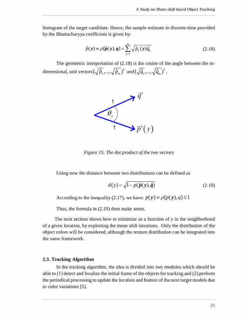
The geometric interpretation of (2.18) is the cosine of the angle between the m-

dimensional, unit vectors 1ˆ ˆ( ,..., )Tmp p and 1 ˆ( ,..., )T

mq q .

Figure 15. The dot product of the two vectors

Using now the distance between two distributions can be defined as

ˆ ˆ( ) 1 ( ( ), )d y p p y q (2.19)

According to the inequality (2.17), we have: ( ) [ ( ), ] 1p p q y y

Thus, the formula in (2.19) does make sense.

The next section shows how to minimize as a function of y in the neighborhood of a given location, by exploiting the mean shift iterations. Only the distribution of the object colors will be considered, although the texture distribution can be integrated into the same framework.

2.3. Tracking Algorithm In the tracking algorithm, the idea is divided into two modules which should be

able to (1) detect and localize the initial frame of the objects for tracking and (2) perform the periodical processing to update the location and feature of the next target models due to color variations [5].


26

2.3.1. Color Representation Target model: Let {x*i}i=1…n be the pixel location of the target model, centered

at 0. We define a function b: R2 {1…m} which associates to the pixel at location xi*

the index b(xi*) of the histogram b in corresponding to the color of that pixel. Thus, the

value of b(xi*) shall be a color value and also the index of the histogram. Many location can have the same b(xi*) color value.

Figure . Illustration of the b(xi*) of the target model

The probability of the color u in the target model is derived by employing a convex and monotonic decreasing kernel profile k which assigns a smaller weight to the locations that are farther from the center of the target. The weighting increases the robustness of the estimation, since the peripheral pixels are the least reliable, being often affected by occlusions (clutter) or background. The radius of the kernel profile is taken equal to one, by assuming that the generic coordinates x and y are normalized with hx and hy, respectively. Hence, we can write [1].

* 2 *

1

ˆ (|| || ) [ ( ) ]n

u i ii

q C k b x u

x (2.20)

Where δ is the Kronecker delta function. The normalization constant C is derived by imposing the condition

1ˆ 1m

uuq

, from where

0

xi b(xi*)

Figure 16. Illustration of the b(xi*) of the target model


27

* 21

1(|| || )n

ii

Ck

x (2.21)

Since the summation of delta function for u=1…m is equal to one.

(a) (b)

Figure 17. Target density function weighting estimation: (a) Triangular Kernel Weighting; (b) Location with same color value

In the figure 17, assume that 1 2 3, ,x x x and 4x are the pixels that have the same feature, such as grey level. Then put them in to the function b would provide the same color value result. Assume that the Kernel estimate function that we used here is Gaussian function. The feature of Gaussian distribution is that the more it is closer to the center the higher the value it get. This could be observed intuitively according to the figure 17. Even though 1 2 3, ,x x x and 4x have the same color value, 2 ,x 4x are more highly weighted in the histogram synthesis process at the index value of b( 1x *) more than 1,x 3x .

Target Candidates: Let 1... hi i nx be the pixel locations of the target candidate,

centered at a calculated location y in the current frame. Similar to the co-ordinate describe in figure 16. However, the center coordinate is y instead of 0. The candidate position can be inferred from the mean-shift vector.


28

Figure 18. Locating the candidate location [13]

Figure 19. Density Estimation Process [13]


29

Using the same kernel profile k, but with radius h, the probability of the color u in the target candidate is given by

2

1

ˆ ( ) [ ]hn

iu h i

ip C k b u

h

y xy x , (2.22)

Where Ch is the normalization constant. The radius of the kernel profile determines the number of pixels (i.e., the scale) of the target candidate. By imposing the condition that we obtain

2

1

1

h

hn ii

Ck

h

y x (2.23)

Note that Ch does not depend on y, since the pixel location xi are organized in a regular lattice, y being one of the lattice nodes. Therefore, Ch can be pre-calculated for a given kernel and different values of h.

2.3.2. Distance Minimization According to Section 3, the most probable location y of the target in the current

frame is obtained by minimizing the distance, which is equivalent to maximizing the Bhattacharyya coefficient ˆ ( )p y . The search for the new target location in the current frame starts at the estimated location 0y of the target in the previous frame. Thus, the

color probabilities 0 1...ˆˆ ( )u u m

p

y of the target candidate at location 0y in the current frame have to be computed first. Using Taylor expansion around the value 0ˆˆ ( )up y , the Bhattacharyya coefficient (17) is approximated as (after some manipulations)

01 1 0

ˆ1 1ˆ ˆ ˆˆ ˆ ˆ( ), ( ) ( )ˆˆ2 2 ( )

m mu

u u uu u u

qp q pp

p y q y yy

(2.24)

Where it is assumed that the target candidate 1...ˆ ( )u u mp

y does not change

drastically from the initial 0 1...ˆˆ ( )u u m

p

y , and that 0ˆˆ ( ) 0up y for all u = 1…m. Introducing now (2.22) in (2.24) we obtain

2

01 1

1ˆ ˆ ˆˆ ˆ( ), ( )2 2

hnmh i

u u iu i

Cp q w kh

y xp y q y (2.25)


30

Where

1 0

ˆ[ ( ) ]

ˆˆ ( )

mu

i iu u

qw b up

xy

(2.26)

Thus, to minimize the distance (2.19), the second term in equation (2.25) has to be maximized, the first term being independent of y. The second term represents the density estimate computed with kernel profile k at y in the current frame, with the data being weighted wi by (2.26). We want to maximize the similarity function of the two distribution. Hence, we need to enlarge the similarity by locating the suitable position y using mean-shift iterations using the following algorithm [5].

Bhattacharyya Coefficient ˆ ˆ( ), p y q Maximization

Given the distribution 1...ˆu u mq

of the target model and the estimated location of

the target in the previous frame:

1. Initialize the location of the target in the current frame with 0y , compute the distribution 0 1...

ˆˆ ( )u u mp

y , and evaluate:

01ˆ ˆ ˆ ˆˆ ˆ( ), ( )m

u uup q

p y q y (2.27)

2. Derive the weights 1...i u mw

according to (25).

3. Based on the mean shift vector, derive the new location of the target (2.14)

20

1

1 20

1

ˆ ˆ

ˆˆ ˆ

h

h

n ii ii

n iii

w gh

w gh

y xxy

y x (2.28)

Update 1 1...ˆˆ ( )u u m

p

y , and evaluate:

1 11ˆ ˆ ˆ ˆˆ ˆ( ), ( )m

u uup q

p y q y

4. While 1 0ˆ ˆ ˆ ˆ ˆ ˆ( ), ( ), p y q p y q (2.29)

Do 1 0 11ˆ ˆ ˆ( )2

y y y

5. If 1 0ˆ ˆ| || y y Stop (2.30)


31

Otherwise Set 0 1ˆ ˆy y and go to Step 1

The proposed optimization employs the mean shift vector in Step 3 to increase the value of the approximated Bhattacharyya coefficient expressed by (2.25). Since this operation does not necessarily increase the value of ˆ ˆ( ), p y q , the test included in Step 4 is needed to validate the new location of the target. However, practical experiments (tracking different objects, for long periods of time) showed that the Bhattacharyya coefficient computed at the location defined by equation (2.28) was almost always larger than the coefficient corresponding to 0y . Less than 0.1% of the performed maximizations yielded cases where the Step 4 iteration were necessary. The termination threshold ε used in Step 5 is derived by constraining the vectors representing 0y and 1y to be within the same pixel in image coordinates.

The tracking consists in running for each time the optimization algorithm described above. Thus given the target model, the new location of the target in the current frame minimizes the distance (2.19) in the neighborhood of the previous location estimate


32

Flow chart:

2.3.3. Scale Adaptation The scale adaptation scheme exploits the property of the distance (2.19) to be

invariant to changes in the object scale. We simply modify the radius h of the kernel profile with a certain fraction (we used +/- 10%), let the tracking algorithm to converge again, and choose the radius yielding the largest decrease in the distance (2.19). An IIR filter is used to derived the new radius based on the current measurement and old radius

Initialize at 0y and calculate q

Start

At the next frame determine 0ˆ( )p y , use mean-

shift vector to find 1y derive weight iw

Determine the similar function

0 01ˆ ˆ ˆ ˆˆ ˆ( ), ( )m

u uup q

p y q y

Find 1ˆ( )p y

Determine the similar function

1 11ˆ ˆ ˆ ˆˆ ˆ( ), ( )m

u uup q

p y q y

1 0ˆ ˆ| || y y

0 11

ˆ ˆˆ2

y yy 0 1ˆ ˆy y

1 0ˆ ˆ( ) ( )y y

TRUE

TRUE

FALSE

FALSE


33

CHAPTER 3: EXPERIMENT RESULT AND EVALUATION

3.1. Testing video a) Ball video

This video contains 3 balls, with 3 different colors, contrast to the background. The balls move with 3 different speeds. In the video, there are time when 3 balls are partially occluded. The frame rate is 25 frames/sec with size 640*480 pixels

b) Street Video

This video contains only one moving object, gray-scale video sequences. The moving speed is quite slow. In the video, there are time when the object changes its shape and appearance. The frame rate is 10 frames/sec with size 320*240 pixels

3.2. Algorithm and demo There are 2 important parts in our experiment that affects a lot to the result: that

is selecting patch and configure the coefficients.

In the figure 20, we show you the window we have designed (in our GUI code) for the selecting patch part. This part provides you the flexibility to choose any object (or area) in interest to track.

Figure 20. Target selection


34

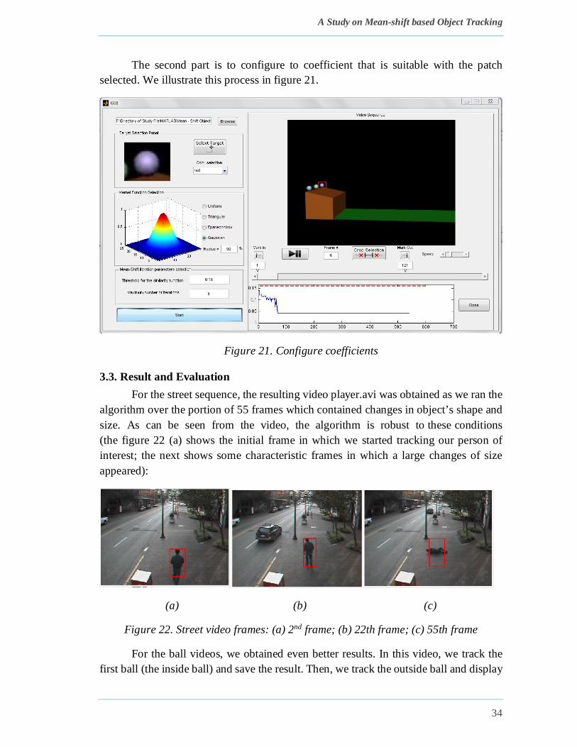
The second part is to configure to coefficient that is suitable with the patch selected. We illustrate this process in figure 21.

Figure 21. Configure coefficients

3.3. Result and Evaluation For the street sequence, the resulting video player.avi was obtained as we ran the

algorithm over the portion of 55 frames which contained changes in object’s shape and size. As can be seen from the video, the algorithm is robust to these conditions (the figure 22 (a) shows the initial frame in which we started tracking our person of interest; the next shows some characteristic frames in which a large changes of size appeared):

(a) (b) (c)

Figure 22. Street video frames: (a) 2nd frame; (b) 22th frame; (c) 55th frame

For the ball videos, we obtained even better results. In this video, we track the first ball (the inside ball) and save the result. Then, we track the outside ball and display


35

both result simultaneously. There are frames in which the inside ball is partially occluded. However, our algorithm manages to keep the inside ball as its target and to avoid occlusion problems.

The problem with the 2 outside balls is that they’re moving too fast. As can be seen in the 22th frame, there was a dramatic change in the outside ball’s speed that made the mean-shift vector for outside ball in 22th frame going the wrong way.

(a) (b) (c)

Figure 23. Ball video frames: (a) 21th frame; (b) 22th frame; (c) 23th frame

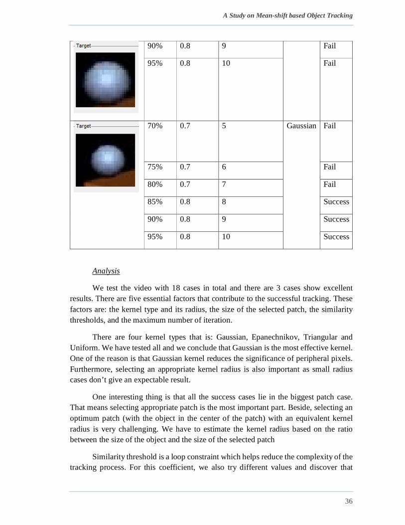
Table 1. The testing table with different parameters.

Select Patch Radius Threshold Max number of iteration

Kernel Result

70% 0.7 5 Gaussian Fail

75% 0.7 6

80% 0.7 7

85% 0.8 8

90% 0.8 9

95% 0.8 10


75% 0.7 6 Fail

80% 0.7 7 Fail

85% 0.8 8 Fail


36

90% 0.8 9 Fail

95% 0.8 10 Fail


75% 0.7 6 Fail

80% 0.7 7 Fail

85% 0.8 8 Success

90% 0.8 9 Success

95% 0.8 10 Success

Analysis

We test the video with 18 cases in total and there are 3 cases show excellent results. There are five essential factors that contribute to the successful tracking. These factors are: the kernel type and its radius, the size of the selected patch, the similarity thresholds, and the maximum number of iteration.

There are four kernel types that is: Gaussian, Epanechnikov, Triangular and Uniform. We have tested all and we conclude that Gaussian is the most effective kernel. One of the reason is that Gaussian kernel reduces the significance of peripheral pixels. Furthermore, selecting an appropriate kernel radius is also important as small radius cases don’t give an expectable result.

One interesting thing is that all the success cases lie in the biggest patch case. That means selecting appropriate patch is the most important part. Beside, selecting an optimum patch (with the object in the center of the patch) with an equivalent kernel radius is very challenging. We have to estimate the kernel radius based on the ratio between the size of the object and the size of the selected patch

Similarity threshold is a loop constraint which helps reduce the complexity of the tracking process. For this coefficient, we also try different values and discover that


37

setting the threshold below 0.4 produce very poor performance. In fact, in most cases, setting the threshold at 0.5 provide the most optimal solution while increasing it slows down the performance.

Similar to the similarity thresholds, the maximum number of iteration should be as high as possible. However, after trying with different values, we observe that the optimum number of iteration is 10 because higher values make no difference in tracking effectiveness but slowing down the performance (longer tracking time).

The final thing we want to talk about is the performance of the algorithm. The sequences were tested, with normal configuration (optimum max iteration number and optimum similarity threshold) on a 2.2 GHz machine with 4000 MB of memory: 55 pedestrian frames took 5 seconds to process, while 120 ball frames took 10 seconds, which is satisfactory, considering that both of these results were obtained within a MATLAB environment. It is assumed that a C implementation could produce much more desirable result


38

CHAPTER 4: DICUSSION AND FUTURE WORK

4.1. Discussion By exploiting the spatial gradient of the statistical measure the mean-shift method

achieves efficient tracking performance, while effectively rejecting background clutter and partial occlusions.

According to Artner, N. M. (2008) [2], Mean-shift is used in color-based object tracking because it is simple and robust. The best results can be achieved if the following conditions are fulfilled:

• The target object is mainly composed of one color.

• The target object does not change its color.

• Illumination does not change dramatically.

• There are no other objects in the scene similar to the target object.

• The color of the background differs from the target object.

• There is no full occlusion of the target object.

The observation of Artner is corresponding to our above video sequences on which the algorithm runs well, thus, providing fully detail about characteristics of mean-shift algorithm.

4.2. Future work One challenge in tracking is to develop algorithms for tracking objects in

unconstrained videos, for example, videos obtained from broadcast news networks or home videos. These videos are noisy, compressed, unstructured, and typically contain edited clips acquired by moving cameras from multiple views. Thus, there is severe occlusion, and people are only partially visible. One interesting solution in this context is to employ histogram of oriented gradient (HOG) in addition to color histogram for object tracking.

The essential thought behind the Histogram of Oriented Gradient descriptors is that local object appearance and shape within an image can be described by the distribution of intensity gradients or edge directions. The implementation of these descriptors can be achieved by dividing the image into small connected regions, called cells, and for each cell compiling a histogram of gradient directions or edge orientations for the pixels within the cell. The combination of these histograms then represents the descriptor. For improved accuracy, the local histograms can be contrast-normalized by calculating a measure of the intensity across a larger region of the image, called a block,


39

and then using this value to normalize all cells within the block. This normalization results in better invariance to changes in illumination or shadowing

Another problem addition is to deal with complete occlusions. One solution is setting a threshold on the similarity coefficient and waiting for a couple of frames, until our target reappears and we have a satisfactory degree of similarity again. This introduces the issue of selecting an optimal threshold on the similarity measure as well as selecting the right number of frames to skip (risking to lose the position of the target).

Finally, to make the algorithm much more efficient, the implementation in C or C++ would be required, thus making the module really applicable to the real-time situations.


40

BIBLIOGRAPHY [1] Alper Yilmaz, Omar Javed, and Mubarak Shah. 2006. Object tracking: A survey. ACM Comput. Surv. 38, 4, Article 13 (December 2006).

[2] Artner, N. M. (2008, April). A comparison of mean shift tracking methods. In 12th Central European Seminar on Computer Graphics (pp. 197-204)

[3] Avidan, S. (2004). Support vector tracking. Pattern Analysis and Machine Intelligence, IEEE Transactions on, 26(8), 1064-1072.

[4] Caulfield, D. (2011). Mean-Shift Tracking for Surveillance: Evaluations and Enhancements.

[5] Comaniciu, D.; Ramesh, V.; Meer, P., "Real-time tracking of non-rigid objects using mean shift," Computer Vision and Pattern Recognition, 2000. Proceedings. IEEE Conference on, vol.2, no., pp.142, 149 vol.2, 2000.

[6] Comaniciu, D.; Ramesh, V.; Meer, P., "Kernel-based object tracking," Pattern Analysis and Machine Intelligence, IEEE Transactions on , vol.25, no.5, pp.564,577, May 2003.

[7] D.W.Scott, Multivariate Density Estimation, New York: Wiley, 1992.

[8] Kailath, T. (1967). The divergence and Bhattacharyya distance measures in signal selection. Communication Technology, IEEE Transactions on, 15(1), 52-60.

[9] Kang, J., Cohen, I., & Medioni, G. (2004, August). Object reacquisition using invariant appearance model. In Pattern Recognition, 2004. ICPR 2004. Proceedings of the 17th International Conference on (Vol. 4, pp. 759-762). IEEE.

[10] T.B. Moeslund, A. Hilton, and V. Kr¨uger. A survey of advances in vision-based human motion capture and analysis. Computer vision and image understanding, 104(2-3):90–126, 2006.

[11] Veenman, C. J., Reinders, M. J., & Backer, E. (2001). Resolving motion correspondence for densely moving points. Pattern Analysis and Machine Intelligence, IEEE Transactions on, 23(1), 54-72.

[12] http://planetmath.org/probabilitydistributionfunction

[13] http://www.wisdom.weizmann.ac.il/~vision/courses/2004_2/files/mean_shift


41

thesis final march

Documents