thesis draft for etd edited - ncsu

ABSTRACT

LYNCH, IYAM IRIE. Friction and Sliding of Polystyrene Micro Particles in the Presence and Absence of Capillary Adhesion. (Under the direction of Dr. Jacqueline Krim.)

This thesis presents the results of a Quartz Crystal Microbalance (QCM) study of how

sample environment (air, nitrogen, vacuum) impacts the form of the friction laws that govern

the polystyrene microparticles deposited onto one of its surface electrodes. Understanding of

friction at both the macro- and nano- scales are far better understood than at this intermediate

(micro) length scale range. Load geometries particularly micro particles are a rapidly

growing field of research. One goal of this thesis was to determine whether the friction

associated with the micron scale particles was similar in nature to typical friction

classifications associated with either scale (Coulomb, granular, viscous, etc.)

The topic has profound implications, given the varied applications in the wide

reaching areas of textiles, biodiagnostics, and nanotransportation. In order to probe the form

of the friction law, studies of the amplitude dependence of particle coupling were performed,

(referred to herein as a “decoupling curve”) monitored both in terms of the QCM response as

well as optically. In order to control, as well as document, the impact of capillary adhesion

on the measurements, an experimental apparatus was designed and constructed to allow

transfer of micro spheres in vacuum from a QCM loaded with spheres to a nearby QCM that

was initially sphere-free. Measurements were performed in air, vacuum, and dry nitrogen,

and the nature of the friction laws was inferred from well- documented QCM frequency

response models. Measurements performed on 5 micron spheres deposited on the surface in

air medium revealed, after an initial drying and “run-in” depinning period, behavior close to

that expected for a physisorbed system governed by a linear viscous friction law. Slip times

for these particles were close to those previously reported for physisorbed water layers.

Measurements performed on dry spheres exhibited far more pronounced decoupling, as well

as a crossover to a friction law closer to conventional Coulomb-type friction observed at

macroscopic length scales. Optical observations showed that the particle motion was

dependent on the oscillation direction and surface topology of the QCM. Particle motion and

dynamics are observed using a microscope with a camera attached. This investigation

documents that the friction and adhesive properties of microspheres are strongly influenced

by the presence or absence of water.

Friction and Sliding of Polystyrene Micro Particles in the Presence and Absence of Capillary Adhesion

by Iyam Irie Lynch

A dissertation submitted to the Graduate Faculty of North Carolina State University

in partial fulfillment of the requirements for the Degree of

Doctor of Philosophy

Physics

Raleigh, North Carolina

2011

APPROVED BY:

_______________________________ ______________________________ Jacqueline Krim David Aspnes Committee Chair ________________________________ ________________________________ Daniel Dougherty Orlando Rojas

ii

DEDICATION

This thesis is dedicated to my grandmother Loretta Campbell for instilling in me the will to

never give up as well as my loving wife Olivia for her constant encouragement.

iii

BIOGRAPHY

Iyam Lynch was born April 7, 1982 at Forsyth Hospital in Winston-Salem, NC. He and his

younger brother Ishum were raised in Mocksville, NC by his grand parents James and

Loretta Campbell. Growing up Iyam was a very curious child who bugged his grandparents

by asking too many questions. He was always active in sports and physical activity however,

he maintained his strong curiosity for understanding how the world worked. It was this

curiosity which led him to pursue physics. In high school Iyam discovered he had a knack

for understanding concepts and most of his courses did not provide too much of a challenge.

This changed when Iyam took a physics course which proved to be both challenging and

humbling. It was then he realized he wanted to take on the challenge of studying this

difficult but wonderfully fundamental discipline. Iyam was not the greatest test taker and his

grades were always above average but nothing outstanding. Despite this fact Iyam was

fortunate enough to obtain acceptance into North Carolina State University under the

transition program. This program was designed to give students of their choosing who were

rejected in the college in which they applied but, their credentials for entering the university

were sufficient. This program was good for Iyam because it required mandatory study hall

and constantly monitored work and grades. After his first semester Iyam received a GPA of

3.8 and was later allowed to matriculate into the physics department. Upon graduating he

decided to stay at NC State to pursue a Ph.D. in physics which had long been his dream. He

was fortunate enough to find a good group that aligned with his interest and personality.

iv

ACKNOWLEDGMENTS

I ultimately realize that with out the help of numerous people I would not even be in a

position to type these sentences on this page. With that said I would first like to

acknowledge my thesis advisor and mentor Dr. Jacqueline Krim whom I respect and admire

for having the patience to deal with me for all these years. I would also like to show my

great appreciation for all of my lab mates past and present who have been extremely helpful

and fun to work with. I would also like to acknowledge Troy Bradshaw, Jessica McNutt,

Andrew Brown, Edward Stevens, and Ben Keller for all of the help they provided me with

collecting data. Lastly, I would like to acknowledge all those individuals who helped keep

my sanity throughout this process my wife Olivia, my family, close friends, and the RDU

Wing Chun School family.

v

TABLE OF CONTENTS

LIST OF TABLES.................................................................................................................... x

LIST OF FIGURES ................................................................................................................. xi

CHAPTER 1: INTRODUCTION............................................................................................. 1

1.1 THE IMPORTANCE OF MICRO-SCALE FRICTION. ............................................... 1

1.2 BIOSENSING APPLICATIONS: THE IMPACT OF FRICTION, ADHESION AND

DECOUPLING ON EMERGING MEDICAL DIAGNOSTIC TECHNIQUES. ................ 2

1.3 THE WORK OF THIS THESIS..................................................................................... 4

1.4 REFERENCES ............................................................................................................... 6

CHAPTER 2: EXPERIMENTAL SETUP ............................................................................... 7

2.1 INTRODUCTION .......................................................................................................... 7

2.2 QUARTZ CRYSTAL MICROBALANCE (QCM) ....................................................... 7

2.2.1 QCM DESIGN......................................................................................................... 8

2.2.2 BASIC QCM THEORY .......................................................................................... 9

2.2.3 THE SAUERBREY RELATION.......................................................................... 12

2.2.4 ELECTRONICS .................................................................................................... 15

2.2.5 MICROSPHERES ................................................................................................. 17

2.2.6 CUSTOMIZED VACUUM CHAMBER .............................................................. 18

2.3 REFERENCES ............................................................................................................. 20

CHAPTER 3: THEORETICAL APPROACHES TO THE ANALYSIS OF QCM

FREQUENCY SHIFT DATA. ............................................................................................... 22

3.1 INTRODUCTION ........................................................................................................ 22

vi

3.2 SLIDING FILMS.......................................................................................................... 23

3.3 THE DYBWAD EXPERIMENT ................................................................................. 28

3.4 QCM CIRCUIT MODEL ............................................................................................. 32

3.5 LIQUID QCM EXPERIMENT .................................................................................... 37

3.6 THE FLANIGAN EXPERIMENT............................................................................... 39

3.7 NEGATIVE SHIFTS, POSITIVE SHIFTS, AND CONTACT AREA ....................... 42

3.8 REVIEW OF “STUDYING MECHANICAL MICROCONTACTS OF FINE

PARTICLES WITH QUARTZ CRYSTAL MICROBALANCE” [32]............................. 49

3.8.1 - 20 MICRON SPHERE SUMMARY................................................................... 54



3.8.4 - 5 MICRON SPHERE SUMMARY..................................................................... 55

3.9 USING A QCM TO DETERMINE THE FRICTION LAW OF LOADING

PARTICLES ....................................................................................................................... 57

3.10 REFERENCES ........................................................................................................... 63

CHAPTER 4 - SPHERE ON FLAT CONTACT MECHANICS........................................... 65

4.1 INTRODUCTION ........................................................................................................ 65

4.2 DRY CONTACTS........................................................................................................ 65

4.2.1 HERTZIAN CONTACT........................................................................................ 65

4.2.3 THE DERJAGUIN APPROXIMATION .............................................................. 67

4.2.2 JKR MODEL ......................................................................................................... 69

4.3 CONTACT MECHANICS IN WET ENVIRONMENTS............................................ 71

vii

4.3.1 CAPILLARY PRESSURE .................................................................................... 71

4.3.2 CAPILLARY CONDENSATION AND FORCES............................................... 73

4.4 REFERENCES ............................................................................................................. 75

CHAPTER 5: FRICTION ANALYSIS OF 5 MICRON POLYSTYRENE SPHERES

DEPOSITED FROM AQUEOUS SOLUTION ON A QUARTZ CRYSTAL

MICROBALANCE ................................................................................................................ 76

5.1 INTRODUCTION ........................................................................................................ 77

5.2 QCM RESPONSE TO LOAD CONFIGURATION AND BEHAVIOR..................... 79

5.3 EXPERIMENTAL SETUP........................................................................................... 83

5.4 METHODS AND MATERIALS.................................................................................. 85

5.5 RESULTS AND DISCUSSION................................................................................... 86

5.6 REFERENCES ............................................................................................................. 97

CHAPTER 6: REDUCING THE EFFECT OF CAPILLARY ADHESION IN QCM

EXPERIMENTS THROUGH IN SITU MICROPARTICAL TRANSFER AND THE

ENVIRONMENTAL DEPENDENCE OF SURFACE DYNAMICS OF POLYSTYRENE

MICROSPHERES ON A QUARTZ CRYSTAL MICROBALANCE .................................. 99

6.1 INTRODUCTION ........................................................................................................ 99

6.2 METHODS AND MATERIALS................................................................................ 101

6.3 PROBING CONTACT MECHANICS WITH A QCM ............................................. 103

6.4 USING DECOUPLING CURVES TO INTERPRET AVERAGE SURFACE

BEHAVIOR...................................................................................................................... 106

6.5 RESULTS AND DISCUSSION................................................................................. 109

viii

6.5.1 DYNAMICS UNDER FLOODED CONDITIONS ............................................ 113

6.5.2 ENVIRONMENTAL INFLUENCE ON FRICTION ......................................... 117

6.5.3 DYNAMICS IN “DRY” CONDITIONS (TRANSFER EXPERIMENT) .......... 123

6.5.4 DYNAMICS IN VARIED ENVIRONMENTAL CONDITIONS...................... 130

6.6 PARTICLE MOTION ................................................................................................ 133

6.7 REFERENCES ........................................................................................................... 139

CHAPTER 7 – STUDIES OF DYNAMICS OF MICROSPHERES IN VARIED FRICTION

REGIMES............................................................................................................................. 141

7.1 WATER DECOUPLING EXPERIMENT IN AIR .................................................... 141

7.2 EXPERIMENT IN AIR OF 15 MICRON SPHERES DEPOSITED FROM AQUEOUS

SOLUTION IN HORIZONTAL ORIENTATION .......................................................... 143

7.2.1 RUN 1 FRICTION ANALYSIS.......................................................................... 145




SOLUTION IN HORIZONTAL ORIENTATION AFTER INTENTIONALLY

DISRUPTING SURFACE BY INDUCING PARTICLE MOTION. .............................. 151


SOLUTION IN VERTICAL ORIENTATION AFTER INTENTIONALLY DISRUPTING

SURFACE BY INDUCING PARTICLE MOTION. ....................................................... 154

ix

7.4.1 EXPERIMENT IN AIR OF 15 MICRON SPHERES DEPOSITED FROM

AQUEOUS SOLUTION IN VERTICAL ORIENTATION AFTER INTENTIONALLY

DISRUPTING SURFACE A SECOND TIME............................................................ 155

7.4.2 FRICTION ANALYSIS OF RUN 1.................................................................... 157



7.5 VARIATION IN MICROPARTICLE COUPLING AS A FUNCTION OF TIME .. 159

7.5.1 15 MICRON SPHERES DEPOSITED FROM AQUEOUS SOLUTION IN AIR

...................................................................................................................................... 161

7.5.2 SINGLE 15 MICRON SPHERE CAUGHT DURING TRANSFER

EXPERIMENT IN 7E-2 TORR VACUUM ENVIRONMENT IN HORIZONTAL

ORIENTATION ........................................................................................................... 162

7.6 REFERENCES ........................................................................................................... 164

CHAPTER 8: CONCLUSIONS AND FUTURE WORK.................................................... 165

8.1 CONCLUSIONS ........................................................................................................ 165

8.2 SUGGESTED FUTURE WORK ............................................................................... 165

x

LIST OF TABLES

Table 3.1- Velocity and slip time values for various friction laws. …………………………61 Table 5.1 - Calculated slip times from forward decoupling curve run. .................................. 89

xi

LIST OF FIGURES

Figure 2.1 - Sketch of experimental apparatus ......................................................................... 7

Figure 2.2 - The AT- Cut9......................................................................................................... 9

Figure 2.3 - QCM front view (a), side view (b), shear mechanical oscillatory response (c)11 . 9

Figure 2.4 - The sound wave propagating through a QCM of thickness T. ........................... 10

Figure 2.5 - Thin film adsorbed on the electrode surfaces of an oscillating QCM ................ 12

Figure 2.6 - Schematic of Pierce oscillator circuit14 ............................................................... 16

Figure 2.7 - Mixer circuit15 ..................................................................................................... 17

Figure 2.8 - Images from left to right 15 micron and 5 micron diameter polystyrene spheres.

.................................................................................................................................... 17

Figure 2.9 - Picture taken of the customized vacuum chamber.............................................. 19

Figure 3.1 - Dybwad’s coupled oscillator model 4 ................................................................. 29

Figure 3.2 - Dybwad’s coupled oscillator extended by arbitrary distances............................ 29

Figure 3.3 - System frequency ω as a function of attachment parameter k.6.......................... 32

Figure 3.4 - Butterworth-Van Dyke equivalent circuit for unloaded QCM. .......................... 33

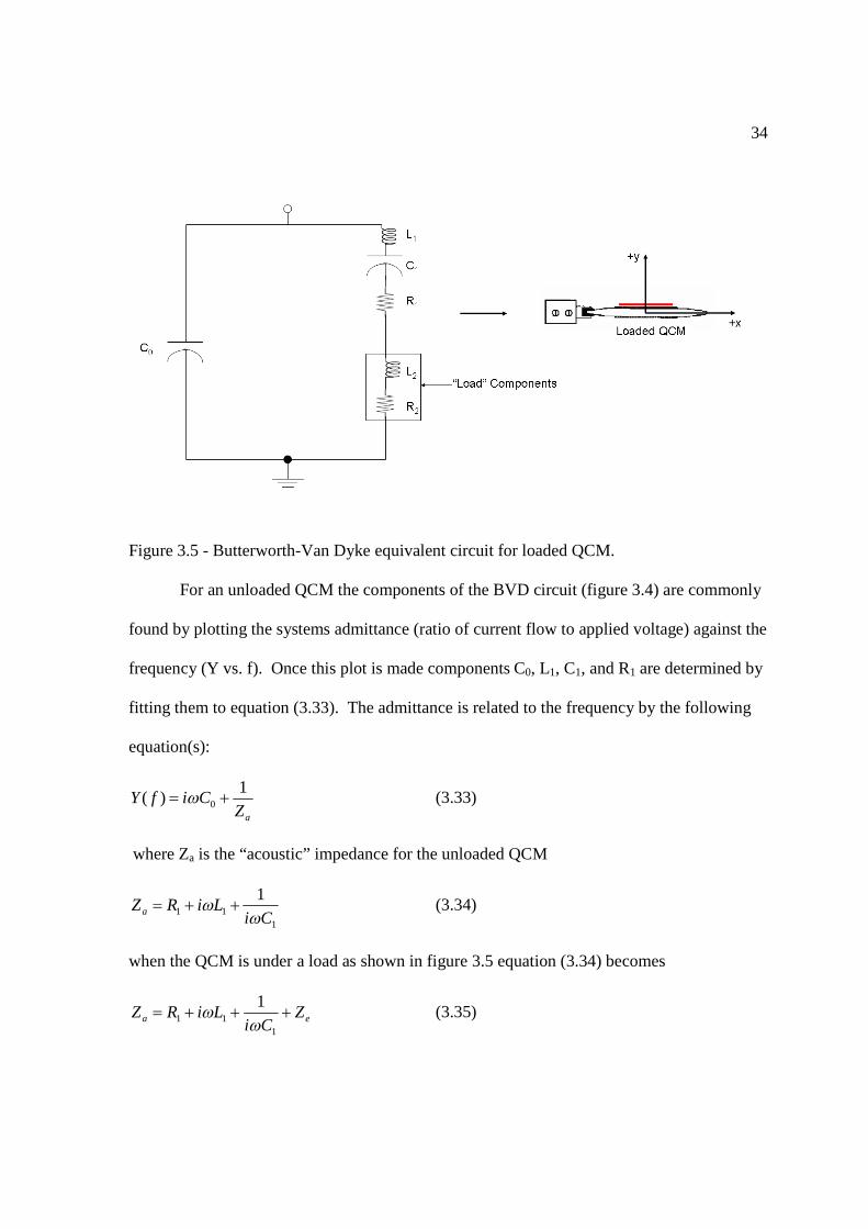
Figure 3.5 - Butterworth-Van Dyke equivalent circuit for loaded QCM. .............................. 34

Figure 3.6 - Flanigan and associates experimental setup12..................................................... 40

Figure 3.7 - Experimental results of Flanigan et. al. Plots show a linear relationship between

frequency shift and contact area of the viscoelastic gel cap12 .................................... 42

Figure 3.8 - A brief summary of QCM frequency shifts for varying load geometries. .......... 43

xii

Figure 3.9 - Lightly coupled sphere on a QCM electrode. The buried contact is magnified to

show that only a few regions or “asperities” are in actual contact. These contact

asperities are highly localized stress regions. ............................................................. 44

Figure 3.10 - Diagram of the experimental setup. .................................................................. 50

Figure 3.11 - System frequency ω as a function of attachment parameter k.6........................ 50

Figure 3.12 - selected QCM experimental results (Fig 6 taken from Ref.18). Drive voltage

was increased to cause a corresponding increase in the oscillation amplitude of the

QCM. Changes in frequency and bandwidth were tracked as the amplitude was

increased. The affects of annealing were monitored in each experiment for the initial

annealing and after a period of time (aged contacts). The experiment was performed

for all size particles. .................................................................................................... 51

Figure 3.13 – 3.13a shows the velocity dependence of various frictional force laws (n). 3.13b

shows the QCM amplitude (velocity) dependence of the slip times (calculating using

n=1) of adsorbed particles (strongly coupled regime) on a QCM. ............................. 58

Figure 3.14 - An illustration of an object set at an initial speed that is subject to a constant

resistive damping force of friction that is velocity dependent. The object shown in this figure

will eventually reach a final velocity of zero as a result of the damping force. The amount of

time the object takes to reach this terminal velocity is dependent on the damping coefficient

and the power law “n” of the damping force. …………………………………………….....60

Figure 3.15- Terminal velocity as a function of slip time for various friction laws. ..………62

Figure 4.1 - Sphere flat geometry under elastic Hertzean contact. ......................................... 67

Figure 4.2 - Sphere on flat geometry in the presence of water ............................................... 72

xiii

Figure 4.3 - Zoomed in image of a microsphere and QCM surface in contact at varying levels

of humidity.................................................................................................................. 73

Figure 5.1 - Depiction of previously studied load geometries of QCM experiments............. 83

Figure 5.2 - Sketch of experimental apparatus. ...................................................................... 85

Figure 5.3 - The image above is a reconstruction of the QCM used in which the initial slip

time was estimated by counting the spheres on the electrode surface before first

oscillation. Each tile is an image with the dimensions of our optical region when

adjusting the resolution to illuminate the spheres on the surface. Scratches were

intentionally placed on the surface to provide a reference point when analyzing the

distance from one image to another when spheres move on the surface. ................... 88

Figure 5.4 -Rresults above were calculated from the slip time values displayed in Table 5.1

for the initial (minimum) drive level and the final (maximum) drive level. .............. 90

Figure 5.5 - (a) in this figure represents an idealized depiction of the QCMs response to in

place particle decoupling or “decoupling curve” in the strong coupling regime of the

Dybwad model. The graph shows no hysteresis because it assumes that particles

return to initial state once crystal amplitude decreases to original drive level. The

graph to the right (b) is the actual experimental data that table 1 is based on. ........... 91

Figure 5.6 - Magnification of runs 1 and 2 from figure 5.5(b) .............................................. 92

Figure 5.7 - Friction analysis of Figure 5.6 decoupling curves. Figure 5.7 (a) is a plot of the

change in frequency from QCM resonance plotted against the crystal amplitude. Run

2 in (a) has been divided into two regions to analyze the change in frictional behavior

associated with the transition between regions. The values of n displayed in (b), (c),

xiv

and (d) correspond with the particle friction law as shown in equation (5.1). These n

values were calculated by applying equation (5.2)..................................................... 93

Figure 6.1 - Schematic of sphere transfer experiment used to reduce the affect of capillary

adhesion from water existing in the buried contact between the QCM electrode and

adsorbed microsphere. In the experiment the 5 MHz or “gun” QCM ejects particles

originally adsorbed from aqueous solution onto the experimental “target” 8 MHz

QCM where data is collected. We chose the 8 MHz QCM as our target due to its

higher sensitivity....................................................................................................... 103

Figure 6.2 - describes the ideal (artificial) situation of decoupling in the strong coupling

regime where a negative shift from fundamental is observed when spheres are

initially applied from mass loading in accordance with the Sauerbrey equation. As

the crystal amplitude is incrementally raised by increasing the drive voltage the

frequency increases as well as a result of effective mass reduction due to sphere

decoupling................................................................................................................. 108

Figure 6.3 - a) displays the QCM response during a decoupling curve experiment, b)the

dependence of crystal amplitude to drive voltage or “signal curve”, and it is linear for

the majority of the experiment.................................................................................. 112

Figure 6.4 - Particle motion observed after rapidly varying the driving voltage. This motion

suggests the bond between the spheres is less than the bond between the spheres and

electrode.................................................................................................................... 112

Figure 6.5 - Image of a QCM in 1 atm Nitrogen while rapidly varying the drive amplitude at

large values to induce particle motion. This QCM had a substantial amount of water

xv

adsorbed onto the surface as a result of the deposition procedure (no drying time). As

a result of the extreme shear forces produced by the QCM the adsorbed layer of water

displayed an extreme amount of mobility................................................................. 113

Figure 6.6 - (a) shows the behavior of the initial decoupling curve performed on this QCM as

well a second decoupling curve followed soon after. The signal curves (b) are

displayed for each data run and show that the oscillation amplitude depended linearly

on the drive voltage from our power supply............................................................. 116

Figures 6.7 - a) and b) are images taken during the initial horizontal orientation decoupling

curve run, these images were taken 3 minutes apart from each other and correspond in

time to the boxed region of the decoupling curve. The increased energy from the rise

in oscillation amplitude from figure 6.7a to 6.7b, aided in breaking the necessary

bonds to translate the circled sphere from the cluster in which it belonged. The

circled sphere is a “first order” or bottom layer sphere that moves roughly in the

oscillation direction................................................................................................... 117

Figure 6.8 - describes the predicted response of the change in QCM frequency to oscillation

amplitude when the adsorbed particles are undergoing a particular frictional

interaction between its contact with the surface. ...................................................... 120

Figure 6.9 - (a) is the change in frequency with respect to crystal amplitude for the

decoupling curve experiment shown in figure 3a. The to plots in (b) are the change in

frequency with respect to crystal amplitude for the “wet” decoupling curve

experiments displayed in figure 6a for the forward runs during the first and second

sweeps. ...................................................................................................................... 121

xvi

Figure 6.10 - Illustrates a mechanism that explains the trend displayed in figures 6.8c and

6.9b run 2 with out the presence of microslip. At increasing amplitude water in the

flooded contact experiences an increase in mobility that draws the microsphere closer

to the substrate increasing the loading force resulting in a negative shift in frequency.

.................................................................................................................................. 122

Figure 6.11 - Image taken after completing a successful transfer experiment. .................... 124

Figure 6.12 - Decoupling curves of the target QCM before and after the transfer experiment

was performed........................................................................................................... 125

Figure 6.13 – Friction analysis of the target QCM after the transfer experiment was

performed.................................................................................................................. 126

Figure 6.14 - Friction analysis of 15 micron microsphere sample deposited from aqueous

solution. The sample was in the strong coupling regime of the Dybwad (SLA) model.

.................................................................................................................................. 127

Figure 6.15 - The image above is a reconstruction of the QCMs used after the transfer

experiment was performed. Each tile is an image with the dimensions of our optical

region when adjusting the resolution to illuminate the spheres on the surface.

Scratches were intentionally placed on the surface to provide a reference point when

analyzing the distance from one image to another when spheres move on the surface.

The highlight region is of a sphere caught near the edge of quartz where the QCM

sensitivity would be minimal. ................................................................................... 128

Figure 6.16 - The above photo consist of two images superimposed onto each other. The first

image is of the surface oriented in the horizontal orientation and the second image is

xvii

after the sample has been rotated in the vertical orientation where gravity has an

affect. We observed particle motion on the rough (quartz) crystal side circled to the

right due to gravity alone whereas no motion was observed for the particles that

landed on the smoother polished gold electrode....................................................... 129

Figure 6.17 - Decoupling curves (forward runs only) for the same sample studied in the

varied environments of air, vacuum (1E-3 torr), and dry nitrogen (N2). The H^2

denotes that the mounting orientation is horizontal or parallel with the surface

(normal to gravity). ................................................................................................... 131

Figure 6.18 -First decoupling curve run in air (approximately 35% r.h.) is shown in (a). The

friction analysis of the forward sweep in the decoupling curve is shown in (b). ..... 131

Figure 6.19 - First decoupling curve run in 1E-3 torr vacuum environment is shown in (a).

The friction analysis of the forward sweep in the decoupling curve is shown in (b).

.................................................................................................................................. 132

Figure 6.20 - Last decoupling curve run in 778 torr dry nitrogen environment is shown in (a).

The frequency shift from resonance of the forward decoupling curve run is shown in

(b). Friction analysis of the forward sweep in the decoupling curve is shown in (c)

and (d). ...................................................................................................................... 133

Figure 6.21 - Dynamics of a partially immersed cluster of aggregated spheres during rapidly

varying the drive voltage of our strong power source. We observed that the shear

stresses were sufficient enough to squeeze water from confined regions within the

cluster........................................................................................................................ 137

Figure 7.1 - Results of water decoupling experiment in air.................................................. 143

xviii

Figure 7.2 - A plot of the water decoupling curve experiment with the forward decoupling

curve runs of the three experiments performed after microspheres were deposited. 144

Figure 7.3 - Friction analysis of the first decoupling curve run ........................................... 145

Figure 7.4 -Ccontinued friction analysis of run 1................................................................. 147

Figure 7.5 - Friction analysis of Run 2 decoupling curve .................................................... 148

Figure 7.6 - Continued friction analysis of Run 2 ................................................................ 149

Figure 7.7 -Friction analysis of Run 3 .................................................................................. 150

Figure 7.8 - Continued friction analysis of Run 3 ................................................................ 151

Figure 7.9 - Decoupling curves after motion generation ...................................................... 153

Figure 7.10 - Decoupling curves before (a) and after (b) motion generation plotted with the

water decoupling experiment.................................................................................... 153

Figure 7.11 - Decoupling curves after placing sample into vertical orientation................... 155

Figure 7.12 - Decoupling curves after disrupting surface in the vertical orientation plotted

with the water decoupling experiment...................................................................... 156

Figure 7.13 - Friction analysis of first decoupling curve run after disrupting surface in the

vertical orientation. ................................................................................................... 157

Figure 7.14 - Friction analysis of second decoupling curve run after disrupting surface in the

vertical orientation .................................................................................................... 158

Figure 7.15 - Friction analysis of fifth decoupling curve run after disrupting surface in the

vertical orientation .................................................................................................... 159

Figure 7.16 - Frequency response over time of a different sample of 15 micron spheres

deposited from aqueous solution. ............................................................................. 161

xix

Figure 7.17 - Frequency response over time of a single15 micron sphere deposited in vacuum

environment. ............................................................................................................. 162

Figure 7.18 - First decoupling curve run of single sphere .................................................... 163

1

CHAPTER 1: INTRODUCTION

1.1 THE IMPORTANCE OF MICRO-SCALE FRICTION.

The notion of transporting micro/nano objects has been of interest to the scientific

community since the early days of nanotechnology. Progress in this area requires an

understanding of the frictional behavior of these objects when they are in motion. Transport

and manipulation of nano and micro devices is a necessary application of both nano/micro

technology that is as intriguing as it is complex. Obtaining this control can lead to many

exciting advancements that span from drug delivery in nanobiotechnology8, micro particle

sorting and grouping by mass5, particle monitoring for toxicological studies as well and many

more favorable applications that span multiple disciplines. However, before these

applications can become a reality several questions must be addressed. What forces

contribute to the friction between the device and surface? How strong are these forces? Can

they be manipulated and if so how? At the micro/nano scale it has been observed in the

literature 9 that particle dynamics are dramatically different than what is seen for the macro

or meso length scales. This is due to the fact that intermolecular and capillary forces become

increasingly important as one approaches these length scales. It was suggested in a previous

study 8 that quartz crystal microbalances (QCMs) could have wide spread potential

applications for separation, sorting, and sizing. In the prior experiments, polystyrene

microspheres were attached to the oscillating surface of a QCM by multiple interactions and

detachment of the spheres from the QCM was achieved by varying the driving voltage of the

QCM. The QCM was oriented horizontally with the spheres deposited on the top side of the

2

electrode. The detachment was inferred by measuring the “sound” the spheres emit upon

detaching with respect to the voltage at which the crystal was being driven. The

experimenters also measured the change in the resonant frequency of the QCM as a function

of the driving voltage. They attributed the changes in frequency of the QCM to be a result of

the spheres detaching from the surface and eventually rolling off the edge of the QCM

causing the mass to decrease which results in a frequency change in the QCM. This

explanation is theoretically sound however, a similar shift in frequency can be observed

when a portion of spheres no longer track the motion of the resonator as a result of surface

decoupling from slipping, sliding, and/or rocking in place in a bound region. In our study we

focus on polystyrene microspheres, which are of growing interest due to their medical and

textile applications. In particular microencapsulation of phase change materials (PCMs)

using polystyrene microspheres, has potential applications toward medical hot/cold therapy

as well as manufacturing clothing to handle extreme weather conditions.10 The topic has also

grown increasingly important in recent years in the biosensing community.

1.2 BIOSENSING APPLICATIONS: THE IMPACT OF FRICTION,

ADHESION AND DECOUPLING ON EMERGING MEDICAL

DIAGNOSTIC TECHNIQUES.

Recent applications involving the use of the quartz crystal microbalance (QCM) are

of growing interest in the biosensor community.1 The QCM provides several advantages in

terms of particle detection. The QCM is low cost and relatively low maintenance in terms of

operation and most importantly is extremely sensitive (can easily detect mass changes on the

3

order of micrograms) to surface changes which makes it ideal for gaining information

regarding contact mechanics2 in a non destructive way. One key advantage the QCM brings

to the biosensor community is its ability to easily distinguish between the weak “non-

specific” surface interactions from the stronger “specific” bonds of study particularly in

complex serums such as blood.1a The use of a QCM also potentially eliminates the need for

tedious labeling procedures during bond rupture scans1b. It has been observed in the

literature3 that varying surface and environmental conditions in particular water layers from

humid air can lead to drastic changes in the binding energy of the particles of study. It has

also been suggested within the biosensing community that the presence of water can result in

unwanted additional effects rising from changes in the acoustic coupling of the adsorbed

liquid layer (interfacial slip) which would cause difficulties during interpretation of data.4

Sensing is not the only issue that is affected by the presence of capillaries from water vapor,

the prospect of micro-sorting via QCM experiments5 would be a cumbersome task in the

presence of water vapor for various reasons. At the microscale inertial loading has little to

no influence on the particles attachment to the surface which means that the particles

adherence to the surface arises primarily from other means such as the van der Waals

interaction and capillary adhesion. It has been observed6 that during QCM experiments

surface particles distributed on the electrode experience non uniform binding energies even

when all surface particles are of the same size and material and deposited under the same

conditions. It is also known7 that the oscillation amplitude of the QCM decreases radially

from the center of the electrode which would have an effect on bond rupture. As a result of

4

these factors it is not guaranteed that adsorbed particles of varying size will sort according to

size alone.

The biosensing community would be well served by a carefully controlled study of the

friction and adhesion of microscale particles. In particular the form of the friction laws that

govern behavior at the micron scale, and how various environmental conditions (air, vacuum,

nitrogen) impact the results.

1.3 THE WORK OF THIS THESIS

As outlined above, this thesis is motivated by a desire to examine how sample

environment, (air, nitrogen, vacuum) impacts the form of the friction laws that govern the

polystyrene microparticles deposited onto the surface electrodes of a QCM. In particular, the

work for this thesis explored whether the friction associated with the micron scale particles

investigated was similar in nature to typical friction classifications associated with classical

friction forms such as Coulomb, granular, viscous, etc. In order to probe the form of the

friction law, studies of the amplitude dependence of particle coupling were performed

(referred to herein as a “decoupling curve”) and monitored both in terms of the QCM

response as well as optically. In order to control, as well as document, the impact of

capillary adhesion on the measurements, an experimental apparatus was designed and

constructed to allow transfer of micro spheres in vacuum from a QCM loaded with spheres to

a nearby QCM that was initially sphere-free. Measurements were performed in air, vacuum,

and dry nitrogen, and the nature of the friction laws was inferred from well- documented

QCM frequency response models. Measurements performed on 5 micron spheres deposited

in air revealed, after an initial drying and “run-in” depinning period, behavior close to that

5

expected for a physisorbed system governed by a linear viscous friction law. Slip times for

these particles were close to those previously reported for physisorbed water layers.

Measurements performed on dry spheres exhibited far more pronounced decoupling, as well

as a crossover to a friction law closer to conventional Coulomb-type friction observed at

macroscopic length scales. Optical observations showed that the particle motion was

dependent on the oscillation direction and surface topology of the QCM. Particle motion and

dynamics were observed using a microscope with a camera attached. As anticipated, this

investigation revealed that the friction and adhesive properties of microspheres were strongly

influenced by the presence or absence of water.

The thesis is organized as follows: The following chapter provides a description of

the experimental chamber and data acquisition procedure. Chapter 3 overviews the various

theories for QCM data analysis based on the assumption of varying forms of the friction laws

assumed to be governing the particle interactions. Chapter 4 overviews the contact mechanics

approaches for asperity contact with an oscillating QCM surface.

Chapters 5 and 6 report respectively a study of the friction law governing 5 micron

spheres in air, and the impact of a dry environment on this law. Chapter 7 describes a unique

investigation of the sliding friction behavior and QCM response to a single 15 micron sphere

located at the center of the QCM electrode. Chapter 8 includes summary comments and

suggestions for future work.

6

1.4 REFERENCES

1. (a) Hirst, E. R.; Yuan, Y. J.; Xu, W. L.; Bronlund, J. E., Bond-rupture immunosensors--A review. Biosensors and Bioelectronics 2008, 23 (12), 1759-1768; (b) Rivet, C.; Lee, H.; Hirsch, A.; Hamilton, S.; Lu, H., Microfluidics for medical diagnostics and biosensors. Chemical Engineering Science 2011, 66 (7), 1490-1507. 2. (a) Dybwad, G. L., A sensitive new method for the determination of adhesive bonding between a particle and a substrate. Journal of Applied Physics 1985, 58 (7), 2789-2789; (b) Flanigan, C. M.; Desai, M.; Shull, K. R., Contact Mechanics Studies with the Quartz Crystal Microbalance. Langmuir 2000, 16 (25), 9825-9829. 3. D'Amour, J. N.; Stålgren, J. J. R.; Kanazawa, K. K.; Frank, C. W.; Rodahl, M.; Johannsmann, D., Capillary Aging of the Contacts between Glass Spheres and a Quartz Resonator Surface. Physical Review Letters 2006, 96 (5), 058301-058301. 4. Ellis, J. S.; Thompson, M., Acoustic physics of surface-attached biochemical species. HFSP Journal 2008, 2 (4), 171-177. 5. Dultsev, F. N.; Ostanin, V. P.; Klenerman, D., “Hearing” Bond Breakage. Measurement of Bond Rupture Forces Using a Quartz Crystal Microbalance. Langmuir 2000, 16 (11), 5036-5040. 6. Vittorias, E.; Kappl, M.; Butt, H.-J.; Johannsmann, D., Studying mechanical microcontacts of fine particles with the quartz crystal microbalance. Powder Technology 2010, 203 (3), 489-502. 7. Seah, P. J. C. a. M. P., The quartz crystal microbalance; radial/polar dependence of mass sensitivity both on and off the electrodes. Measurement Science and Technology 1990, 1 (7), 544-555. 8. Medvedeva, N. V. I., O.M.; Ivanov, Yu. D.; Drozhzhin, A.I.; Archakov, A.I., Nanobiotechnology and nanomedicine. Biomeditsinskaya Khimiya 2006, 52 (6), 529-546. 9. Peri, M. D. M.; Cetinkaya, C., Rotational motion of microsphere packs on acoustically excited surfaces. Applied Physics Letters 2005, 86 (19), 194103-194103. 10. Sánchez, L.; Sánchez, P.; Lucas, A.; Carmona, M.; Rodríguez, J. F., Microencapsulation of PCMs with a polystyrene shell. Colloid and Polymer Science 2007, 285 (12), 1377-1385.

7

CHAPTER 2: EXPERIMENTAL SETUP

2.1 INTRODUCTION

One of the main purposes of our experimental design is to drastically reduce and/or

eliminate capillary forces on the micro particles. Elimination/reduction of these forces

greatly simplifies the analysis and also allows controlled comparisons to be performed in the

presence and absence of capillary effects. An additional benefit of this setup is the ability to

compare results in two different particle environments, dry and humid. Our design also

allows us to study particle motion in both vertical and horizontal orientations which permits

examination of the impact of gravity on particle motion and friction.

Figure 2.1 - Sketch of experimental apparatus

2.2 QUARTZ CRYSTAL MICROBALANCE (QCM)

QCM is the main experimental tool used in our experiments. In particular we employ

two QCM’s operating at very different frequencies (8 MHz and 5 MHz) to eliminate “cross

talk” created by beat frequencies between the two QCM’s. The following section provides

an overview of the basic ideas underlying the design and operation of a QCM.

Oscillator Circuit

Sample

Microscope + CCD Camera

Frequency Counter + Multimeter

Computer

Power Supply 25 microns

25 microns

8

2.2.1 QCM DESIGN

Historically the QCM’s were developed as timer components, and later adapted as

“microbalances” to monitor film thickness and mass per unit area during gas uptake or thin

film deposition.1 They have since been adapted for a wide variety of more diverse

applications2,3,4,5,6,7. A QCM is comprised of two main components, a precisely cut wafer of

quartz and two conducting electrodes that are deposited on the top and bottom portions of the

quartz wafer. The functional component of the QCM is the quartz wafer. Quartz is a

crystalline form of SiO2 and a piezoelectric material, which means that when a voltage is

applied to the quartz it will respond mechanically. When the conducting electrodes are

attached to the top and bottom of the quartz wafer, an alternating voltage can be applied to

the plates to produce an oscillatory response in shear mode within it. The crystal will

oscillate at its fundamental (or overtone) frequency, which is determined by the thickness of

the wafer. A QCM has the favorable properties of high frequency stability as well as a high

“quality factor” (Q) which is the ratio of energy stored to energy lost in the resonator per

cycle. The manner in which a QCM is cut has a major impact on the fundamental properties

of the oscillator, in particular the frequency, stress, and temperature dependence8. In our

experiments we used AT cut crystals which are oriented 35 degrees 15 minutes with respect

to the ZX crystal plane as shown in the figure below.

9

Figure 2.2 - The AT- Cut9 as shown in 2.2b the cut is made along the zx axis.

The AT cut crystal that we employ operate with low temperature sensitivity (highest

frequency stability and mass sensitivity) at room temperature. Our QCM(s) diameter was

0.375 and had a 0.01 inch flat on the –x axis was used to label the direction of oscillation.

The crystals oscillated in the fundamental (8MHz and 5MHz) mode and had an optical

(overtone) polished finish. The electrode was keyhole design with a diameter of 0.250 inches

and it was made from gold deposited atop a thin chrome adhesion layer. Our QCM’s where

purchased from Laptech Precision Inc out of Ontario Canada10.

Figure 2.3 - QCM front view (a), side view (b), shear mechanical oscillatory response (c)11

2.2.2 BASIC QCM THEORY

In this section I review basic ideas discussed in the previous sections. I first discuss how the

frequency of the QCM is determined by the thickness of the quartz disc and how that

10

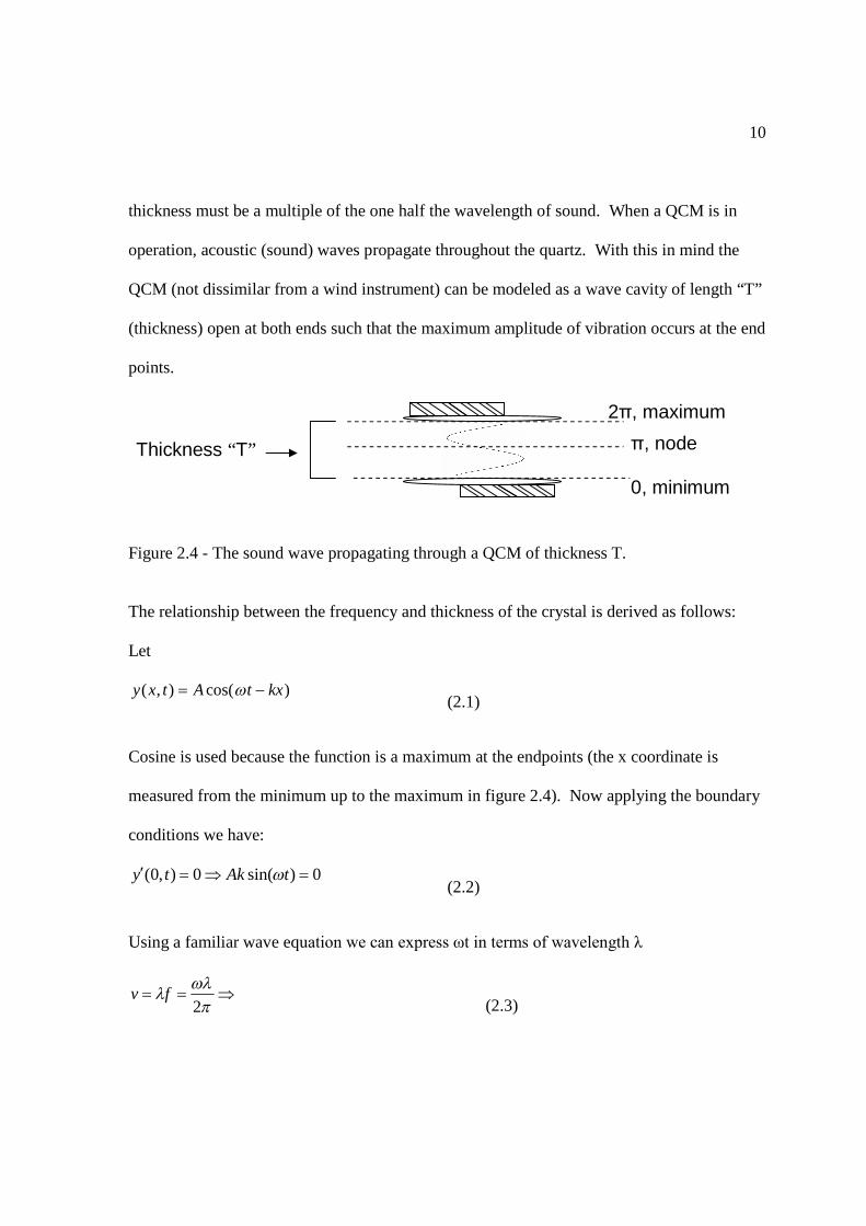
thickness must be a multiple of the one half the wavelength of sound. When a QCM is in

operation, acoustic (sound) waves propagate throughout the quartz. With this in mind the

QCM (not dissimilar from a wind instrument) can be modeled as a wave cavity of length “T”

(thickness) open at both ends such that the maximum amplitude of vibration occurs at the end

points.

Figure 2.4 - The sound wave propagating through a QCM of thickness T.

The relationship between the frequency and thickness of the crystal is derived as follows:

Let

)cos(),( kxtAtxy -= w (2.1)

Cosine is used because the function is a maximum at the endpoints (the x coordinate is

measured from the minimum up to the maximum in figure 2.4). Now applying the boundary

conditions we have:

0)sin(0),0( =Þ=¢ tAkty w (2.2)

Using a familiar wave equation we can express ωt in terms of wavelength λ

Þ==p

wll2

fv (2.3)

0, minimum

Thickness “T”

2π, maximum

π, node

11

Þ=lpw v2

(2.4)

lp

lpw )(22 txvt

t == (2.5)

Applying the boundary condition (2.2) we have

0)sin( =tw (2.6)

,...2,1,0,2

===Þ nnx

t plpw (2.7)

,22mx

nx

==ppl (2.8)

,...3,2,1=® mn n is replace with m to avoid divergence Thus

2lm

x = (2.9)

Setting x equal to the “thickness” T we obtain the following relations

2maxlm

T = (2.10)

Tmvv

f ss

2==

l (2.11)

where sv is the velocity of sound through quartz and maxl is the maximum wavelength of a

sound wave propagating through quartz. This derivation provides information on the

relationship between QCM frequency (fundamental and higher modes “overtones”) and

thickness. It also shows the dependence a QCM’s thickness has on the wavelength of sound.

12

The next section will elaborate on the QCM’s sensitive dependence on changes in thickness,

which is the heart of the approximation made when applying the QCM as a mass sensor.

2.2.3 THE SAUERBREY RELATION

The “microbalance” moniker for the QCM has its origins with the Sauerbrey7

relation. The QCM has a narrow bandwidth and a high quality factor (Q) which makes its

frequency of oscillation very sensitive to small changes in mass or more accurately thickness.

The Sauerbrey7 equation relates the change in QCM mass resulting from the deposition of a

uniform thin film on the electrode surface to the change in the QCM’s frequency from

resonance. The derivation assumes that the mass is rigidly attached to the motion of the

QCM and as a result can be considered as an effective increase in the thickness of the quartz

itself. This assumption works quite well for sufficiently thin films.12

The following figure is a schematic demonstrating the problem that Sauerbrey wished

to solve. In particular, Sauerbrey examined the shift in frequency of the resonator when a

uniform thin layer of mass adsorbed to one side of the QCM surface.

Figure 2.5 - Thin film adsorbed on the electrode surfaces of an oscillating QCM

Sauerbrey assumes equation (2.10), (2.11)

13

,2

maxlmT = (2.12)

Tmvv

f ss

2==

l (2.13)

Using the fundamental mode we set m=1

Tv

f s

2= (2.14)

Since we are interested in how the frequency changes with thickness we will differentiate the

above expression:

( ) ÷øö

çèæ

¶¶

+¶¶

= -

21

21 ss v

TTT

Tv

Tf

dd

(2.15)

To a good approximation δvs/δT = 0 since the mass film is thin and rigidly attached.

Applying this approximation yields the following result

Tf

tv

Tf s 0

22-

=-

=dd

(2.16)

Separating variables we have

TT

ff dd -

=0

(2.17)

We now need to relate the change in quartz thickness with the change in mass (to one side of

the QCM) using the density of quartz (ρq).

Þ= ATm qq r (2.18)

A

mT

q

q

r=

(2.19)

14

AmT

qrdd 1

= (2.20)

Now applying the most important approximation that

qf mm << (2.21)

qfqtotal mmmm »+= (2.22)

fmm »d (2.23)

Plugging this approximation into equation (2.20) yields an equation that relates the change in

quartz thickness to the mass of the adsorbed film mf

A

m

Am

Tq

f

q rrdd == (2.24)

We wish to express the frequency shift from resonance in terms of change in mass.

Combining the earlier equations (2.16) and (2.17) will accomplish this goal.

q

f

m

m

TT

ff -

=-

=dd

0 (2.25)

00 fAT

mf

m

mf

q

f

q

f

rd

-=

-= (2.26)

Finally solving the earlier expression T

vf s

20 = (2.14) for vs and plugging the result in the

previous equation we obtain the Sauerbrey equation for mass adsorbed to one side of the electrode.

20

2f

A

m

vf f

sq÷÷ø

öççè

æ-=

rd (2.27)

15

2.2.4 ELECTRONICS

The QCM was driven by a Pierce oscillator circuit whose output signal was mixed

using a 0.5 to 500 MHz frequency mixer with a reference signal supplied by an 8 MHz can

crystal oscillator driven by a different Pierce oscillator circuit. The mixed output ran through

a low pass filter and was detected using a Hewlett Packard 5384A frequency counter. The

crystal amplitude was measured using a Keithley 2000 multimeter. The reference “can”

QCM was powered by an Elenco Precision model XP-15 regulated variable power supply

and the experimental 8 MHz QCM was driven with a Keithley 2400 digital source meter. A

second Keithley 2400 digital source meter was used to drive a 5 MHz QCM in experiments

where both the 8 MHz and 5MHz crystal were oscillating simultaneously in close range.

These source meters are extremely low noise instruments which allowed us to make accurate

measurements while varying the drive voltage of one of the crystals. Below is a diagram of

the Pierce oscillator circuit. The Pierce circuit was a convenient choice to power our crystals

for several reasons. The Pierce oscillator operates well in the presence of high stray

capacitances resulting from various mounting arrangements as well as maintaining high

frequency stability even for low drive levels13.

16

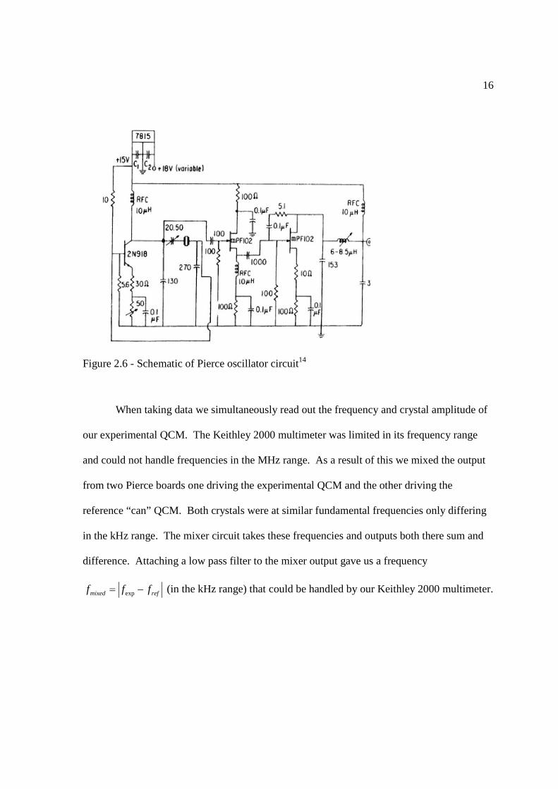
Figure 2.6 - Schematic of Pierce oscillator circuit14

When taking data we simultaneously read out the frequency and crystal amplitude of

our experimental QCM. The Keithley 2000 multimeter was limited in its frequency range

and could not handle frequencies in the MHz range. As a result of this we mixed the output

from two Pierce boards one driving the experimental QCM and the other driving the

reference “can” QCM. Both crystals were at similar fundamental frequencies only differing

in the kHz range. The mixer circuit takes these frequencies and outputs both there sum and

difference. Attaching a low pass filter to the mixer output gave us a frequency

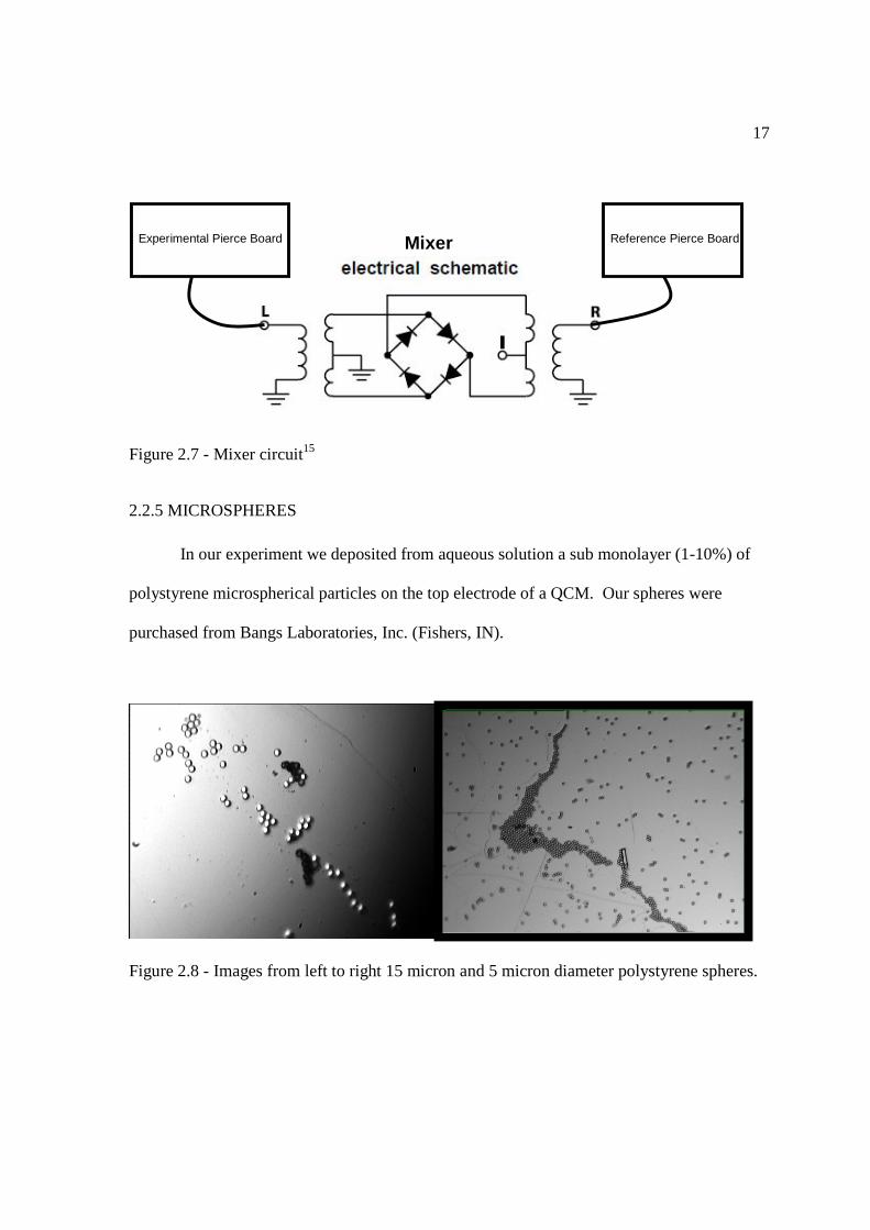
refmixed fff -= exp (in the kHz range) that could be handled by our Keithley 2000 multimeter.

17

Figure 2.7 - Mixer circuit15

2.2.5 MICROSPHERES

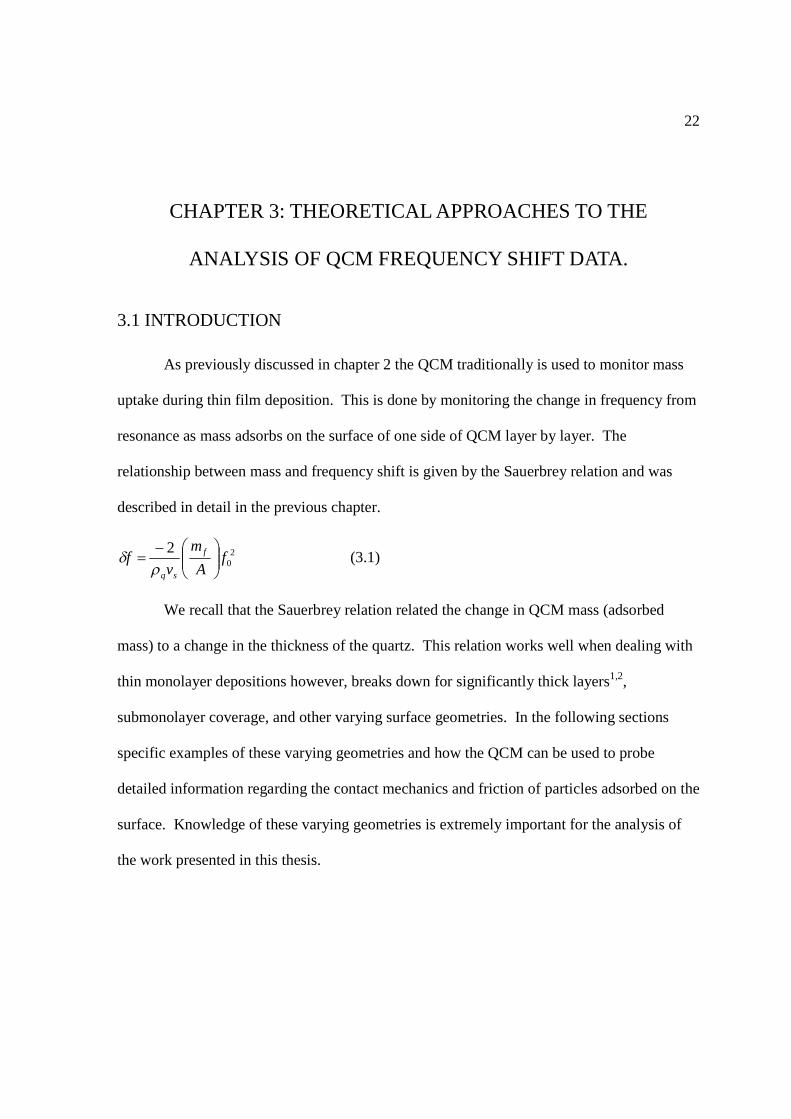
In our experiment we deposited from aqueous solution a sub monolayer (1-10%) of

polystyrene microspherical particles on the top electrode of a QCM. Our spheres were

purchased from Bangs Laboratories, Inc. (Fishers, IN).

Figure 2.8 - Images from left to right 15 micron and 5 micron diameter polystyrene spheres.

Experimental Pierce Board Reference Pierce Board Mixer

18

2.2.6 CUSTOMIZED VACUUM CHAMBER

Experiments were performed in a vacuum chamber customized to rotate

approximately 270 degrees in order to perform experiments in both vertical and horizontal

orientations along with all angles in between. The horizontal and vertical experiments were

both performed in the following environments: air, vacuum, and dry nitrogen. Inside of the

chamber are two QCM holders one oriented in the horizontal plane while the other is

oriented in the vertical plane with respect to the acceleration of gravity. These holders were

placed in such a way to allow sphere transfer experiments to be performed in situ. Transfer

experiments were performed by depositing microspheres on the 5 MHz QCM which were to

be placed in the vertical holder. We then placed a blank 8 MHz QCM in the horizontal

holder located directly below the vertical holder. Spheres were transferred by generating

particle motion on the QCM in the vertical holder by strongly driving and rapidly varying the

applied voltage. The projected particles landed on the oscillating 8 MHz QCM which was

held at a fixed voltage. The choice of 5 and 8 MHz QCMs was chosen to eliminate “cross

talk” from beat frequencies produced from the QCMs. Eliminating the cross talk allowed us

to record QCM behavior during particle transfer. Particle motion was analyzed using an

Edmund optics Proximity Series Infinitube microscope with a Mitutoyo 10X/0.28 lens

illuminated by an Edmund Industrial Optics model 21AC illuminator. Attached to the

microscope was a B/W CCD camera from Industrial Vision Source whose video output was

sent to the computer program Flash Point 3D and a Toshiba DVD recorder to record movies

of surface motion.

19

Figure 2.9 - Picture taken of the customized vacuum chamber.

The data recorded in this setup were analyzed in terms of both the frequency shift data and

the optical information obtained with the camera. In the next chapter, I will describe the

various theoretical approaches employed for analysis of frequency shift data, including

analysis treatments of quality factor shifts when relevant.

20

2.3 REFERENCES

1. King, W. H., Piezoelectric Sorption Detector. Analytical Chemistry 1964, 36 (9), 1735-1739. 2. Dultsev, F. N.; Ostanin, V. P.; Klenerman, D., “Hearing” Bond Breakage. Measurement of Bond Rupture Forces Using a Quartz Crystal Microbalance. Langmuir 2000, 16 (11), 5036-5040. 3. Dybwad, G. L., A sensitive new method for the determination of adhesive bonding between a particle and a substrate. Journal of Applied Physics 1985, 58 (7), 2789-2789. 4. Flanigan, C. M.; Desai, M.; Shull, K. R., Contact Mechanics Studies with the Quartz Crystal Microbalance. Langmuir 2000, 16 (25), 9825-9829. 5. Krim, J.; Widom, A., Damping of a crystal oscillator by an adsorbed monolayer and its relation to interfacial viscosity. Physical Review B 1988, 38 (17), 12184-12184. 6. Laschitsch, A.; Johannsmann, D., High frequency tribological investigations on quartz resonator surfaces. Journal of Applied Physics 1999, 85 (7), 3759-3759. 7. Sauerbrey, G., Verwendung von Schwingquarzen zur Wägung dünner Schichten und zur Mikrowägung. Zeitschrift für Physik 1959, 155 (2), 206-222. 8. Varma, M. R. Vapor Phase Lubrication of Microelectro Mechanical Systems(MEMS): An Atomistic Approach to Solve Friction and Stiction in MEMS. North Carolina State University, Raleigh, 2003. 9. Crystallographic quartz axes figure reference. 10. Laptech Precision Inc, Part # XL1018, http://www.laptech.com. 11. Robbins, M. O., Energy Dissipation in Interfacial Friction. Krim, J., Ed. MRS Bulletin: MRS Bulletin, 1998; Vol. 23, pp 23-26. 12. Vogt, B. D.; Lin, E. K.; Wu, W.-l.; White, C. C., Effect of Film Thickness on the Validity of the Sauerbrey Equation for Hydrated Polyelectrolyte Films. The Journal of Physical Chemistry B 2004, 108 (34), 12685-12690. 13. Abdelmaksoud, M. Nanotribology of a Vapor Phase Lubricant: Quartz Crystal Microbalance Study of Tricresylphosphate (TCP) Uptake on Iron and Chrome North Carolina State University, Raleigh, 2001.

21

14. Winder, S. M. North Carolina State University, Raleigh, 2003. 15. Mini-Circuits, Mini-Circuits Frequency Mixer SRA-1 Data Sheet.

22

CHAPTER 3: THEORETICAL APPROACHES TO THE

ANALYSIS OF QCM FREQUENCY SHIFT DATA.

3.1 INTRODUCTION

As previously discussed in chapter 2 the QCM traditionally is used to monitor mass

uptake during thin film deposition. This is done by monitoring the change in frequency from

resonance as mass adsorbs on the surface of one side of QCM layer by layer. The

relationship between mass and frequency shift is given by the Sauerbrey relation and was

described in detail in the previous chapter.

20

2f

A

m

vf f

sq÷÷ø

öççè

æ-=

rd (3.1)

We recall that the Sauerbrey relation related the change in QCM mass (adsorbed

mass) to a change in the thickness of the quartz. This relation works well when dealing with

thin monolayer depositions however, breaks down for significantly thick layers1,2,

submonolayer coverage, and other varying surface geometries. In the following sections

specific examples of these varying geometries and how the QCM can be used to probe

detailed information regarding the contact mechanics and friction of particles adsorbed on the

surface. Knowledge of these varying geometries is extremely important for the analysis of

the work presented in this thesis.

23

3.2 SLIDING FILMS

Equation (3.1) from the previous section assumes that the adsorbed mass is rigidly

attached to the QCM electrode. As a result of the extreme shear vibrations the adsorbed

particles experience on the electrode surface it is not hard to imagine the possibility of

interfacial slip. When slip occurs on the surface, equation (3.1) is no longer a valid means of

measuring mass due to the additional effects particles slipping on the surface have on the

QCM. In 1986 researchers Krim and Widom3 realized this possibility and developed

methods to quantify the friction between the QCM electrode and the sliding “decoupled”

particles. To address this behavior the researchers used a combination of fluid dynamics and

driven oscillator mechanics to describe the experimental situation. To understand their

methodology we examine the different ways a QCM can be modeled. The most common

ways to model a QCM are as an equivalent circuit or a mass-spring system although other

methods do exist (optical and purely mathematical) 4. Krim and Widom modeled the QCM

as a driven mass-spring system with damping. Writing out the sum of all the forces

(considered) for this system gives:

mm C

xxRxmtF ++= &&&)cos(0 w (3.2)

Assuming solutions have the form

)()( dw -= tiAetx (3.3)

Then the velocity is written as

( )mmm CMiRF

vww /1--

= (3.4)

24

Where mR , mM , mC , and w are the mechanical resistance, mass, compliance (1/(spring

constant k), and frequency respectively and δ represents the phase angle. Equation (3.2) has

obvious parallels with an RLC electrical circuit driven by and alternating emf V. For this

system the mechanical impedance is

)/1( mmmmmm CMiRiXRvF

Z ww --=-== . (3.5)

The term mX is the mechanical reactance of the system and is proportional to the

inertial components of the system and mR is proportional to the energy dissipation (loss) of

the system. The authors realized that a QCM under a particular load would experience some

increase in the impedance (3.5) of the system. If the components of the impedance mR and

mX could be computed in terms of the properties of the loading material then detailed

information regarding the behavior of the particles on the QCM surface could be extracted in

particular whether the surface particles were rigidly attached or decoupled (sliding). In cases

where the Sauerbrey equation (3.1) apply the resistive term of equation (3.5) would go to

zero and the entire contribution of the impedance of the system would be inertial however,

for systems where the films begin to decouple and slide the resistive term is greater than

zero. In order to understand how a 2D film affects the impedance of a QCM it is beneficial

to first examine the effect of a 3D fluid (or gas) interacting with the QCM. For a fluid

interacting with an oscillating plane (QCM) the Navier-Stokes relation is sufficient to

describe the behavior.

25

2

2

33 zv

tv xx

¶¶

=¶

¶ hr , (3.6)

where 3r is the density of the 3D fluid, xv is the velocity of the QCM in the x-direction such

that ( )tvvx wcos0= , and 3h is the bulk viscosity of the 3D fluid. The 2D film adsorbed onto

the surface of the QCM from the surrounding 3D fluid will have the following equation of

motion,

ff vdtvd 22 )/( hfr -Ñ-= (3.7)

where 2h , 2r ,f , and fv are the 2D film viscosity, density, spreading pressure, and velocity

respectively. A 2D adsorbed monolayer film has a spreading pressure equal to zero thus it is

implied from equation (3.7) that

ò ò-= ff vdAdtvddA 22 )/( hr . (3.8)

The classical shear impedance is found from the solution of equation (3.8)

33333 )1( hrpfiiXRZ -=-= (3.9)

where 3Z is the acoustical shear impedance which is equivalent to the mechanical impedance

( )mZ per unit area. In order to compensate for excess momentum fluctuations resulting from

gas particles with velocity components commensurate with the oscillation of the QCM the

authors have replaced the viscosity term in equation (3.9) with the complex viscosity

úû

ùêë

é-

=riwt

hh1

13

*3 (3.10)

26

where rt is the time it takes for the excess particle momentum to relax to 1/e of its initial

equilibrium value. Taking into consideration equation (3.10) the components for equation

(3.9) become,

( )

2/1

233*3 1

11

1 ïþ

ïýü

ïî

ïíì

úû

ùêë

é+÷÷

ø

öççè

æ+

+=

rr

rfRwtwt

wthrp (3.11)

( )

2/12/1

233*3 1

11

1 ïþ

ïýü

ïî

ïíì

úúû

ù

êêë

é-÷÷

ø

öççè

æ+

+=

rr

rfXwtwt

wthrp . (3.12)

Equations (3.11) and (3.12) can be used to find the “excess dissipation per unit mass”

from the momentum fluctuations of the 3D gas to the QCM surface. This is done by taking

the ratio of (3.11) to (3.12) in the limit 1<<rwt (short relaxation times) as shown in

equation (13) below

rXR wt+=1*

3

*3 . (3.13)

For a 2D adsorbed film which is what we are mainly concerned with the authors

found a similar expression for the ratio of the 2D counterparts of equation (3.13)

wt=*2

*2

XR

. (3.14)

where t in (3.14) is the characteristic “slip time” or the time it takes for an adsorbed film to

stop once slipping has begun. This term is analogous to the relaxation time introduced for

the 3D fluid damping case. The authors discuss how the case of a film rigidly attached to the

motion of the QCM (equation (3.1)) is an approximation of the actual situation of slip. When

a film obeys equation (3.1) the slip time is much smaller than the period of oscillation of the

27

QCM thus slip is not observable. However, when the slip time is commensurate with the

period of oscillation of the QCM the effects of slip can be probed via the added impedance to

the QCM. The authors rigorously showed an agreement between the classical result of (3.14)

and a result obtained from a quantum mechanical approach. They found the following

results for the components of the added impedance a QCM experiences from a 2D adsorbed

film on one side

( ),

1 2

22*

2 wttwr

+=R

(3.15)

where 2r is mass per unit area of the 2D adsorbed layer, in g/cm2

( )22*

21 wt

wr+

=X (3.16)

where the ratio of (3.15) to (3.16) is in agreement with (3.14). As stated earlier the real and

imaginary components of the impedance an adsorbed film adds to a QCM are related to the

dissipative and inertial properties respectively. These expressions were derived by

Stockbridge 5 and are

,21 *

qqtR

Q wrd =ú

û

ùêë

é (3.17)

,*

qqtX

rdw = (3.18)

where úû

ùêë

éQ1d is the shift in inverse quality factor or “change in dissipation” of the system,

dw is the shift from resonance and qt is the thickness of quartz. Plugging (3.15) and (3.16)

28

into (3.17) and (3.18) and taking the ratio of (3.17) to (3.18) the authors found the central

result of their work which was an expression of slip time in terms of measurable changes in

the QCM during deposition.

tdwd 21

=úû

ùêë

éQ

(3.19)

Plugging (3.16) into (3.18) gives the frequency shift from resonance the QCM

experiences from film slippage.

( )21 wtd

d+

= filmff (3.20)

In equation (3.20) filmfd is the shift in frequency from mass loading (no slipping) and is

therefore found by applying equation (3.1).

3.3 THE DYBWAD EXPERIMENT

In 1985 Dybwad performed an experiment where he placed a single gold microsphere

on the center portion of an oscillating QCM 6. He observed a positive shift in frequency

which at first glance appears contradictory to the Sauerbrey equation. Similar to the authors

from section 3.2, Dybwad modeled the QCM as a mechanical system. He explained his

result by modeling the single sphere QCM geometry as a coupled mechanical oscillator. By

doing so he justified the possibility of measuring a positive shift in frequency when a single

particle is “lightly” coupled to the electrode of the QCM. This experiment was one of the

first examples of how a QCM could be used to probe particle adhesion.

29

Figure 3.1 - Dybwad’s coupled oscillator model 4

Using figure 3.1 I will review Dybwad’s published result for the system’s frequency response

as a function of the single sphere “attachment parameter” )(kw .

We begin by displacing each object in the coupled oscillator model by an arbitrary

distance as shown in figure 3.2.

Figure 3.2 - Dybwad’s coupled oscillator extended by arbitrary distances.

where M is the mass associated with the QCM, m is the mass of the sphere deposited to one

side of the QCM, K is the spring constant associated with the QCM, and k is the spring

constant of the sphere which is also referred to as the “attachment parameter” a value that

describes the bond strength between the sphere and QCM surface. After applying this

30

displacement we write the equations of motion for objects M and m via Newton’s 2nd law

assuming x2 larger than x1.

)( 1211 xxkKxxM -+-=&& (3.21)

)( 122 xxkxm --=&& (3.22)

01211 =+-+ xMk

xMk

xMK

x&& (3.23)

0122 =-+ xmk

xmk

x&& (3.24)

The differential equations (3.22) and (3.23) can be solved by assuming the following

solutions for x1 and x2.

)cos(11 tCx w= (3.25)

)cos(22 tCx w= (3.26)

Since we are searching for the normal mode frequencies of this coupled oscillator system the

frequency term ω must be the same for both equations (3.25) and (3.26). It is also necessary

that there are exactly two normal mode solutions since there are two objects (QCM and

single microsphere). Plugging (3.25) and (3.26) into (3.23) and 3. (24) we obtain:

Mk

CMk

MK

C 22

1 )( =++-- w (3.27)

mk

Cmk

C 12

2 )( =+-w (3.28)

We now have 2 equations (3.27) and (3.28) with 3 unknown variables C1, C2, and ω.

To solve this problem we must have 3 equations. The third equation comes from finding the

ratio of the amplitudes 21 / CC . When solving this ratio for equations (3.27) and (3.28) then

31

equating the two expressions we effectively eliminate the ratio. The result is an expression

for frequency as a function of “attachment parameter” ω(k).

÷øö

çèæ

÷øö

çèæ +-

=÷øö

çèæ ++-

÷øö

çèæ

=

mk

mk

Mk

MK

Mk

CC

2

22

1

w

w (3.29)

After some algebra, one arrives at the following expression from equation (3.29)

024 =+÷øö

çèæ ++-

MmKk

mk

Mk

MKww . (3.30)

Equation (3.30) is a quadratic equation that leads to two solutions (negative

frequencies have no physical meaning) for the normal modes of the coupled oscillator

system. Applying the quadratic equation to solve Equation (3.30), we obtain:

22

24 w=

-±-a

acbb, where

MmKk

c

mk

Mk

MK

b

a

=

÷øö

çèæ ++-=

=1

(3.31)

After applying equation (3.31) we arrive at Dybwad’s expression for )(kw , where m is the

mass of a particle added on one side of the crystal.

.42

2/122

úúû

ù

êêë

é-÷

øö

çèæ ++±÷

øö

çèæ ++=

mk

MK

mk

Mk

MK

mk

Mk

MKw (3.32)

Plotting the system frequency ω as a function of the attachment parameter k, Dybwad

obtined the idealized behavior of the coupled system. This plot is shown in figure 3.3 where

two coupling regimes, “strong” and “weak”, are highlighted. In the strong region (large k

values) the plot shows negative values for the frequency in accordance with equation (3.1).

32

Conversely in the weak region (small k values) the plot shows that when the sphere is

“loosely” attached to the QCM, positive shifts in frequency are possible. This is a result of

the additional “stiffness” the system experiences from the bond. In other words the bond is

not strong enough for the sphere to track the motion of the QCM so the resonator does not

detect its mass (inertial loading) however, it can sense the added stiffness from the sphere-

electrode bond.

Figure 3.3 - System frequency ω as a function of attachment parameter k.6

3.4 QCM CIRCUIT MODEL

We next consider a theoretical treatment of the QCM that models it in terms of its

equivalent electrical components, which can then be related back to the mechanical

properties of the crystal. An unloaded QCM oscillating at or near resonance can be modeled

as a Butterworth-Van Dyke equivalent circuit as shown in figure 3.4. The Butterworth-van

Dyke (BVD) circuit is an approximation of the more rigorous Mason equivalent circuit 7.

33

Figure 3.4 - Butterworth-Van Dyke equivalent circuit for unloaded QCM.

The term C0 is the “shunt” capacitance and is a combination of the static capacitance

between electrodes on both sides of the quartz and the “parasitic” capacitance that arises

from external sources such as mounting. The right side of figure 3.4 is sometimes referred to

as the “acoustic branch” and is composed of additional inductive, capacitive, and resistive

(L1, C1, and R1 respectively). The terms from the acoustic branch arise from electric

coupling to the shear mechanical displacement resulting from oscillation. When a QCM is

loaded by some external means (film deposition, liquid loading, microspheres deposited on

surface, etc.) the system experiences additional impedance to its motion and is interpreted in

the BVD model as load components. These components are pictured in figure 3.5.

34

Figure 3.5 - Butterworth-Van Dyke equivalent circuit for loaded QCM.

For an unloaded QCM the components of the BVD circuit (figure 3.4) are commonly

found by plotting the systems admittance (ratio of current flow to applied voltage) against the

frequency (Y vs. f). Once this plot is made components C0, L1, C1, and R1 are determined by

fitting them to equation (3.33). The admittance is related to the frequency by the following

equation(s):

aZCifY

1)( 0 += w (3.33)

where Za is the “acoustic” impedance for the unloaded QCM

111

1Ci

LiRZa ww ++= (3.34)

when the QCM is under a load as shown in figure 3.5 equation (3.34) becomes

ea ZCi

LiRZ +++=1

11

1w

w (3.35)

35

where Ze is the electrical load impedance and is written as

22 LiRZ e w+= (3.36)

The electrical load impedance is directly proportional to the load impedance ZL that

results from the contact between the load material and the QCM surface. When LZ is small

compared to the shear wave impedance of quartz, qqqZ rm= , it has been shown8 that

÷÷ø

öççè

æ=

q

Le Z

ZCK

NZ

0024 w

p (3.37)

where N is the overtone order (N=1,3,5,…), 00 2 fpw = where 0f is the undamped resonant

frequency of the QCM and K2 is the AT-cut quartz electromechanical coupling factor and is

equal to 31074.7 -´ according to Ballato9. The load impedance ZL is defined by the ratio of

the shear stress of the loading material to the shear velocity of the load at the QCM boundary.

0=

=yx

xyL v

Zs

(3.38)

where xys is the shear stress (force per unit area in x-direction normal to y-direction see

figure 3.5) to the load material from the oscillation of the QCM and xv is the corresponding

shear velocity of the load particles.

It is important to note that ZL is a complex quantity and the real component Re(ZL)

represents the mechanical power dissipation and corresponds to the stress component in

phase with the particle velocity. The imaginary component Im(ZL) is the stress component

90 degrees out of phase with the particle velocity and corresponds to the mechanical energy

36

storage at the surface. If it is possible to find (3.38) then the “load” components from (3.36)

can be found. Combining (3.36) and (3.37) gives:

q

L

ZZ

CKN

R)Re(

4 0022 w

p= (3.39a)

q

L

ZZ

CKN

L)Im(

4 020

22 wp

= (3.39b)

From equations (3.39a) and (3.39b) we observe that knowledge of the load impedance

gives all the information required to calculate the electrical impedance Ze of the loaded

QCM. Information from these components are used to interpret interfacial properties of the

system such as adhesion and friction 3. It is useful to write out expressions for changes in

frequency and bandwidth in terms of ZL as we will see later on. To do so we begin by

writing the series resonant frequency fs in terms of the acoustic and load components.

021 )(2

1

CLLfs +

=p

(3.40)

Changes in L2 lead to changes in fs thus the change in frequency Δf can be

approximated as:

1

02

2LfL

f-

=D (3.41)

I will now write out the expressions for the unloaded “acoustic” components L1, C1,

and R1 as shown by Martin et al 10.

( )0

20

2

2

1 8 CKN

Lwp

= (3.42a)

)(8

20

2

1 pNCK

C = (3.42b)

37

( )q

q

CKN

Rmhp

02

2

1 8= (3.42c)

In equations (3.42a-c) the term ηq is the viscosity of quartz and the term C0 varies

from the term in figures 3.4 and 3.5 in that it does not take into consideration the “parasitic”

capacitance from external sources and is purely the capacitance between the electrode plates

such that q

q

h

AC 0

0

e= where qe is the permittivity of quartz, 0A is the active region of the

electrode, and qh is the thickness of quartz. Substituting (3.39b) and (3.42a) into equation

(3.41) we obtain the frequency shift in terms of the load impedance LZ .

q

L

ZZ

Nf

f)Im(0

p-=D (3.43)

where equation (3.43) represents the frequency shift for one side of the QCM.

3.5 LIQUID QCM EXPERIMENT

In some applications mass adsorption on the QCM is performed in liquid medium.

When a QCM is submerged in a fluid it experiences additional changes in its amplitude and

frequency that must be subtracted from the effects adsorption. The frequency shift from

resonance of a QCM taken from air and submerged into a Newtonian liquid was derived in

1985 by Kanazawa and Gordon 11.

The liquid decay length for a critically damped shear wave originating from the

QCM’s oscillating surface and migrating into the contacting layer of a Newtonian liquid is

given by the following equation 2.

38

2/1

0

2÷÷ø

öççè

æ=

l

l

rwhd (3.44)

where lh is the viscosity of the surrounding liquid, lr is the density of the surrounding

liquid, and 00 2 fpw = is the angular resonant frequency of the QCM. If we assume that the

thickness of the liquid layer coupled to the motion of the QCM is δ/2, and apply the

following substitutions (3.45) to the Sauerbrey equation (3.1)

( )

2

2

sqq

fl

v

A

m

rm

dr

=

÷÷ø

öççè

æ®

(3.45)

we obtain the following expression:

2/1

2/30

2/12/30

÷÷ø

öççè

æ-=÷

øö

çèæ-

=qq

llll

sq

fv

ff

mprhr

phr

rd (3.46)

Equation (3.46) is known as the Kanazawa-Gordon relation where ρl and ηl are the

density and viscosity of the surrounding liquid. The values in the denominator of equation

(3.46) are intrinsic properties of AT- cut quartz density ρq=2.651 g/cm3 and shear stiffness

µq= 1110947.2 ´ dyn/cm2. Equation (3.46) can also be found using the BVD circuit model

described in the previous section. The velocity field from the QCM generated into a semi

infinite Newtonian fluid is 2

÷øö

çèæ +

= yi

vyv xx d)1(

exp)( 0 . (3.47)

From (3.47) the shear stress xys for this system is

39

( )jvyv x

y

xxy +=

¶¶

-==

10

0d

hhs (3.48)

using thickness equal to δ/2 and plugging )43()38()48( ®® we obtain the Kanazawa-

Gordon equation (3.46).

3.6 THE FLANIGAN EXPERIMENT

Another example of how a QCM can be used to probe contact mechanics is an

experiment performed by Flanigan et. al. in the year 2000. In this experiment they used a

QCM in conjunction with an axisymmetric adhesion test apparatus to obtain calibrations

between the frequency change of the crystal and the corresponding contact area of a

viscoelastic gel cap pressed against the crystal surface 12. Their analysis was a combination

of the JKR contact mechanics model 13 along with the previously mentioned Kanazawa-

Gordon and Sauerbrey equations. Their overall goal was to show how a QCM along with a

displacement sensor can be used to measure adhesion energy according to the JKR contact

mechanics model. They demonstrated how a QCM can be used to acquire contact area

directly without monitoring the contact area between the gel and electrode surface 12. They

found a linear relationship between the QCMs resonant frequency and the gel/electrode

contact area. This is true provided that the contact area is confined to the central portion of

the QCM where the amplitude and sensitivity is largest 8.

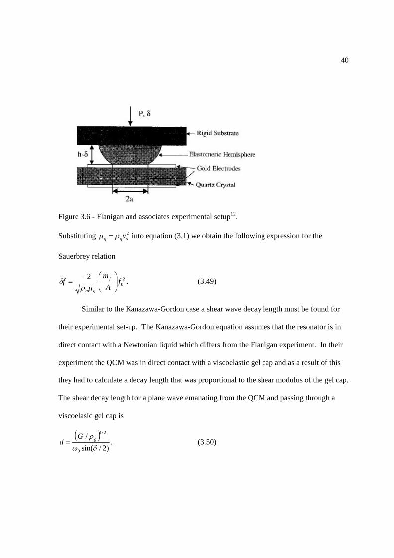
40

Figure 3.6 - Flanigan and associates experimental setup12.

Substituting 2sqq vrm = into equation (3.1) we obtain the following expression for the

Sauerbrey relation

20

2f

A

mf f

qq÷÷ø

öççè

æ-=

mrd . (3.49)

Similar to the Kanazawa-Gordon case a shear wave decay length must be found for

their experimental set-up. The Kanazawa-Gordon equation assumes that the resonator is in

direct contact with a Newtonian liquid which differs from the Flanigan experiment. In their

experiment the QCM was in direct contact with a viscoelastic gel cap and as a result of this

they had to calculate a decay length that was proportional to the shear modulus of the gel cap.

The shear decay length for a plane wave emanating from the QCM and passing through a

viscoelasic gel cap is

( ))2/sin(

/

0

2/1

dwrgG

d = . (3.50)

41

where gr is the density of the gel cap, G is the magnitude of the complex shear modulus of

the gel, and the complex shear modulus is dieGGiGG =¢¢+¢=* . When o902/ == pd is

plugged into the complex shear modulus the entire contribution is from gG hw0=¢¢ and

equation (3.50) reduces to the decay length for a Newtonian liquid (3.44) where gh is the

viscosity of the gel but, for the case of o902/ == pd it reduces to the viscosity of a

Newtonian liquid. Substitution of ÷÷ø

öççè

æ®

=A

md fgrd

2)90( o

in equation (3.49) results in (3.46)

as expected from the previous section. Flanigan and coworkers applied this method for

phase angles (δ) less than o90 to approximate the effects of viscoelasticity. Using equation

(3.50) for d and applying ÷÷ø

öççè

æ®

<A

md fgrd

2)90( o

in equation (3.49) gives:

.)2/sin(2

2/1

0

÷÷ø

öççè

æ-=

qq

gGff

mrr

dpd (3.51)

The researchers realized that their work was not yet done since equation (3.51)

assumes that the gel is in contact with the entire electrode. To address this issue they inserted

a sensitivity factor into equation (3.51) and showed results for the two extreme cases.

( ).

)2/sin(2/

0

2/1

00÷÷ø

öççè

æ÷÷ø

öççè

æ-=

AAGAAKf

fqq

g

mrr

dpd (3.52)

A in equation (3.52) is the “active area” or the area of the gel in direct contact with the QCM

electrode. 0A is the area of the entire electrode and ( )0/ AAK is the sensitivity factor. The

first extreme case is ( ) 11 =K which is in accordance with equation (3.51) the next extreme

42

case is where a very small amount of the gel is in contact with the electrode. This case was

worked out by Lin et. al. 14 and the sensitivity factor is ( ) 20 »K . Plugging this result into

(3.52) gives:

)2/sin(

2/1

dd GK

Af g-

= (3.53)

where

2/1

0

0

÷÷ø

öççè

æ-=

qq

gg A

fK

mrr

p (3.54)

Equation (3.53) represents the slope of frequency shift from resonance plotted against

the contact area of the gel cap. This theoretical model is supported by figure 3.7.

Figure 3.7 - Experimental results of Flanigan et. al. Plots show a linear relationship between

frequency shift and contact area of the viscoelastic gel cap12.

3.7 NEGATIVE SHIFTS, POSITIVE SHIFTS, AND CONTACT AREA

Figure 3.8 outlines the overall effect loading a QCM in a particular way has on the resonant

frequency. One of three things happens to the resonant frequency of a QCM when an

43

object(s) interacts with its surface, the frequency either: decreases, increases, or remains the

same.

Figure 3.8 - A brief summary of QCM frequency shifts for varying load geometries.

From figure 3.8 we see that cases a, b, d, and e are geometries that result in a negative

shift from resonance. Negative shifts in frequency are well understood when the QCM is

modeled with plane waves. We first encountered this in Chapter 2 when working out the

QCM’s frequency dependence to the thickness of the cut. We assumed that “sound” moved

through the QCM in a transverse shear mode as a plane wave, this was also the case for

liquid loading (Kanazawa-Gordon) and viscoelastic materials (Flanigan). Generally speaking

large contacts (uniform thin films and “soft” viscoelastic materials) result in negative shifts

in frequency whereas small contacts result in positive shifts from resonance. A contact is

considered small when the actual radius of the contact (rc) is much smaller than the local

44

radius of contact (R) and the wavelength of sound (λ) 4. When this is the case there is a

stress concentration at the point of contact and it is assumed 15 that a spherical wave is

emitted into the QCM that increases the “stiffness” (“k” value) of the oscillator. It is also

possible for there to be no change in frequency, this is usually the case for purely elastic

materials. In section 3.3 I rigorously worked out the result of Dybwad which shows the

possibility of measuring a positive shift from resonance when a single particle is “lightly”

coupled to the active area of the QCM. Dybwad’s experiment is a classic example of how

point contacts affect the resonant frequency of a QCM and his result can be replicated by

using the BVD model discussed in section 3.7.

Figure 3.9 - Lightly coupled sphere on a QCM electrode. The buried contact is magnified to

show that only a few regions or “asperities” are in actual contact. These contact asperities

are highly localized stress regions.

Researchers Laschitsch and Johannsmann pointed out that if the size or radius cr of

the contact pictured in figure 3.9 is much smaller than the wavelength of sound λ then the

wave transmitted into the sphere can be approximated as spherical15. Knowing the form of

wave emitted into the sphere provides a starting point for evaluating the expected shift in

frequency from this type of load geometry. Assuming that there is just one elastic modulus

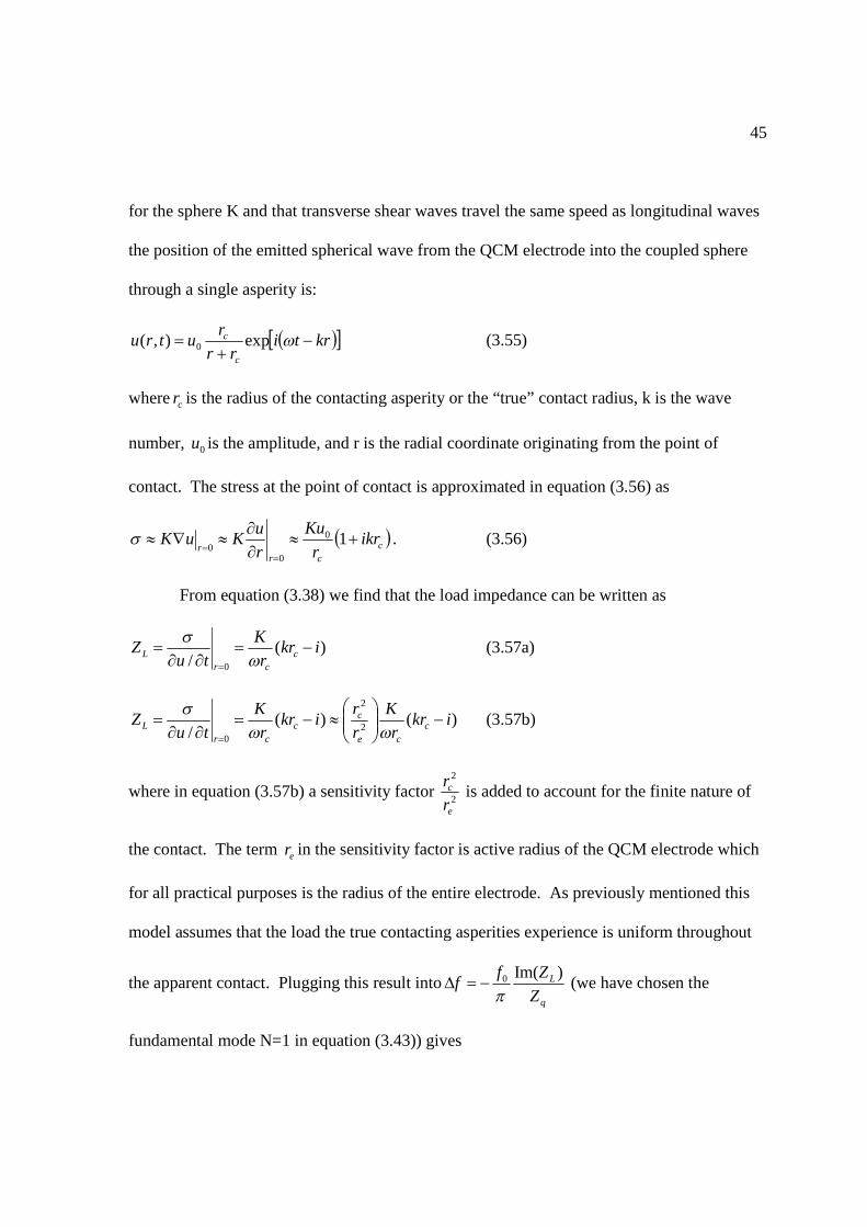
45

for the sphere K and that transverse shear waves travel the same speed as longitudinal waves

the position of the emitted spherical wave from the QCM electrode into the coupled sphere

through a single asperity is:

( )[ ]krtirr

rutru

c

c -+

= wexp),( 0 (3.55)

where cr is the radius of the contacting asperity or the “true” contact radius, k is the wave

number, 0u is the amplitude, and r is the radial coordinate originating from the point of

contact. The stress at the point of contact is approximated in equation (3.56) as

( )ccr

rikr

rKu

ru

KuK +»¶¶

»Ñ»=

=10

00

s . (3.56)

From equation (3.38) we find that the load impedance can be written as

)(/ 0

ikrr

Ktu

Z ccr

L -=¶¶

== w

s (3.57a)

)()(/ 2

2

0

ikrr

Krr

ikrr

Ktu

Z cce

cc

crL -÷÷

ø

öççè

æ»-=

¶¶=

= wws

(3.57b)

where in equation (3.57b) a sensitivity factor 2

2

e

c

rr

is added to account for the finite nature of

the contact. The term er in the sensitivity factor is active radius of the QCM electrode which

for all practical purposes is the radius of the entire electrode. As previously mentioned this

model assumes that the load the true contacting asperities experience is uniform throughout

the apparent contact. Plugging this result intoq

L

ZZf

f)Im(0

p-=D (we have chosen the

fundamental mode N=1 in equation (3.43)) gives

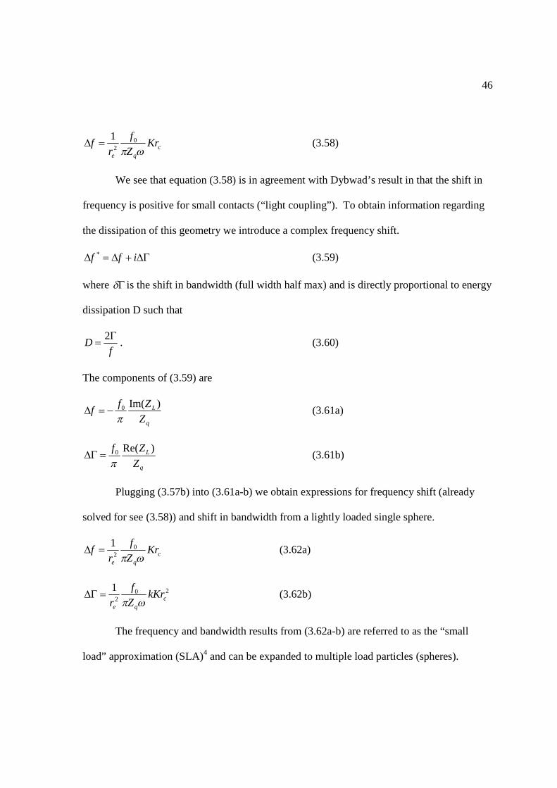
46

cqe

KrZf

rf

wp0

2

1=D (3.58)

We see that equation (3.58) is in agreement with Dybwad’s result in that the shift in

frequency is positive for small contacts (“light coupling”). To obtain information regarding

the dissipation of this geometry we introduce a complex frequency shift.

DG+D=D iff * (3.59)

where Gd is the shift in bandwidth (full width half max) and is directly proportional to energy

dissipation D such that

fD

G=

2. (3.60)

The components of (3.59) are

q

L

ZZf

f)Im(0

p-=D (3.61a)

q

L

ZZf )Re(0

p=DG (3.61b)

Plugging (3.57b) into (3.61a-b) we obtain expressions for frequency shift (already

solved for see (3.58)) and shift in bandwidth from a lightly loaded single sphere.

cqe

KrZf

rf

wp0

2

1=D (3.62a)

202

1c

qe

kKrZf

r wp=DG (3.62b)

The frequency and bandwidth results from (3.62a-b) are referred to as the “small

load” approximation (SLA)4 and can be expanded to multiple load particles (spheres).

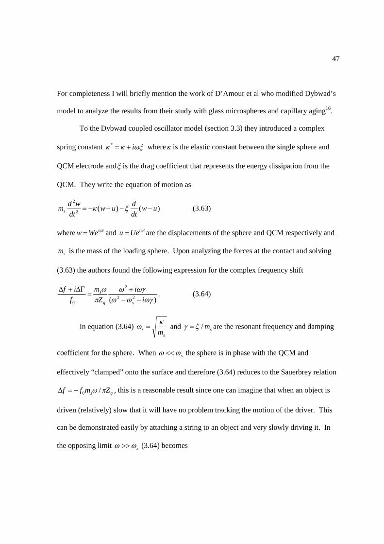
47

For completeness I will briefly mention the work of D’Amour et al who modified Dybwad’s

model to analyze the results from their study with glass microspheres and capillary aging16.

To the Dybwad coupled oscillator model (section 3.3) they introduced a complex

spring constant wxkk i+=* wherek is the elastic constant between the single sphere and

QCM electrode andx is the drag coefficient that represents the energy dissipation from the

QCM. They write the equation of motion as

)()(2

2

uwdtd

uwdt

wdms ----= xk (3.63)

where tiWew w= and tiUeu w= are the displacements of the sphere and QCM respectively and

sm is the mass of the loading sphere. Upon analyzing the forces at the contact and solving

(3.63) the authors found the following expression for the complex frequency shift

)( 22

2

0 wgwwwgw

pw

ii

Zm

fif

sq

s

--+

=DG+D

. (3.64)

In equation (3.64) s

s mkw = and sm/xg = are the resonant frequency and damping

coefficient for the sphere. When sww << the sphere is in phase with the QCM and

effectively “clamped” onto the surface and therefore (3.64) reduces to the Sauerbrey relation

qs Zmff pw /0-=D , this is a reasonable result since one can imagine that when an object is

driven (relatively) slow that it will have no problem tracking the motion of the driver. This

can be demonstrated easily by attaching a string to an object and very slowly driving it. In

the opposing limit sww >> (3.64) becomes

48

2 00

ss

q q

m ff f

Z Zw k

p w p wD = = (3.65a)

00

s

q q

m ff

Z Zwg g

p w pDG = = (3.65b)

these equations are equivalent to the expressions worked out using the BVD model equations

(3.62a-b) where cKrµk . Equations (3.65a-b) are reasonable since they are in the limit

where the loading particle is unable to track the extreme oscillation of the driver and

therefore is not “detected” by the resonator. This condition is exactly that of light coupling

(Dybwad) and leads to positive shifts in frequency. In figure 3.8 the geometry of an SFM

(surface force microscopy) probe15, 17 interacting with a QCM pictured in (f) is well

described in the SLA approximation. In the next section I will review an article18 that uses

the SLA equations (3.62a-b) and (3.65a-b) as its main form of analysis. The geometry of this

experiment is closely related to the work reported in this thesis. Another experiment closely

related to the topic of this thesis is that of Dultsev et al19. This geometry is pictured in figure

3.8 (d) and labeled beside it is a negative shift in frequency. This shift was true for the

experiment performed by the authors however, positive shifts have been observed as well for

the geometry shown in figure 3.8 (d)16, 18. Geometries involving microspheres of varying

sizes and distributions on a QCM have shown varied shifts in resonant frequency when

initially placed on the QCM6, 16, 18 which suggest that the initial conditions of the deposition

procedure are important. We have seen from the various forms of the Dybwad model that

the contact area and overall adhesion or (coupling constant) dictate which way the frequency

will go once the particles are deposited. The variation in behavior suggest that differences in

the environment (dry or wet) during the deposition procedure as well as the roughness of the

49

particles can have a major affect on the initial contact area and adhesion of the particles to

the QCM surface.

3.8 REVIEW OF “STUDYING MECHANICAL MICROCONTACTS OF

FINE PARTICLES WITH QUARTZ CRYSTAL MICROBALANCE” [32]

The aim of the research reported in this article was to analyze the adhesion of glass

microspherical particles, in particular how the adhesion is affected by QCM experiments.

The researchers studied three different particle diameters (5µm, 10µm, and 20µm) in order to

vary the inertial and contact forces. The particles were deposited on a thin polystyrene (PS)

layer that was spin coated on the surface of the electrode. Particle adhesion was increased by

annealing the PS layer at Co150 which formed a PS meniscus. Experiments were performed

by tracking changes in the frequency and bandwidth of the QCM as the oscillation amplitude

was increased. Initial runs were performed on QCM’s with the PS layer alone to test the

range of oscillation amplitudes allowed to perform the experiment. If the oscillation

amplitude was too high the polystyrene film would decouple and slip (see section 3.2) on the

surface which would distort the researcher’s data. To prevent this they performed their

experiments well below this limit. The entire process was observed via optical spectroscopy

as shown in figure 3.10.

50

Figure 3.10 - Diagram of the experimental setup.

A semi-quantitative analysis was performed by applying the Dybwad model (3.64) to

multiple contacts and using SLA equations (3.65a-b). Particles where placed in one of two

categories “strong” or “weak” coupling. Strange behavior in their results was explained by

the particles being in the intermediate coupling regime where behavior is hard to predict as

shown by figure 3.11.

Figure 3.11 - System frequency ω as a function of attachment parameter k.6

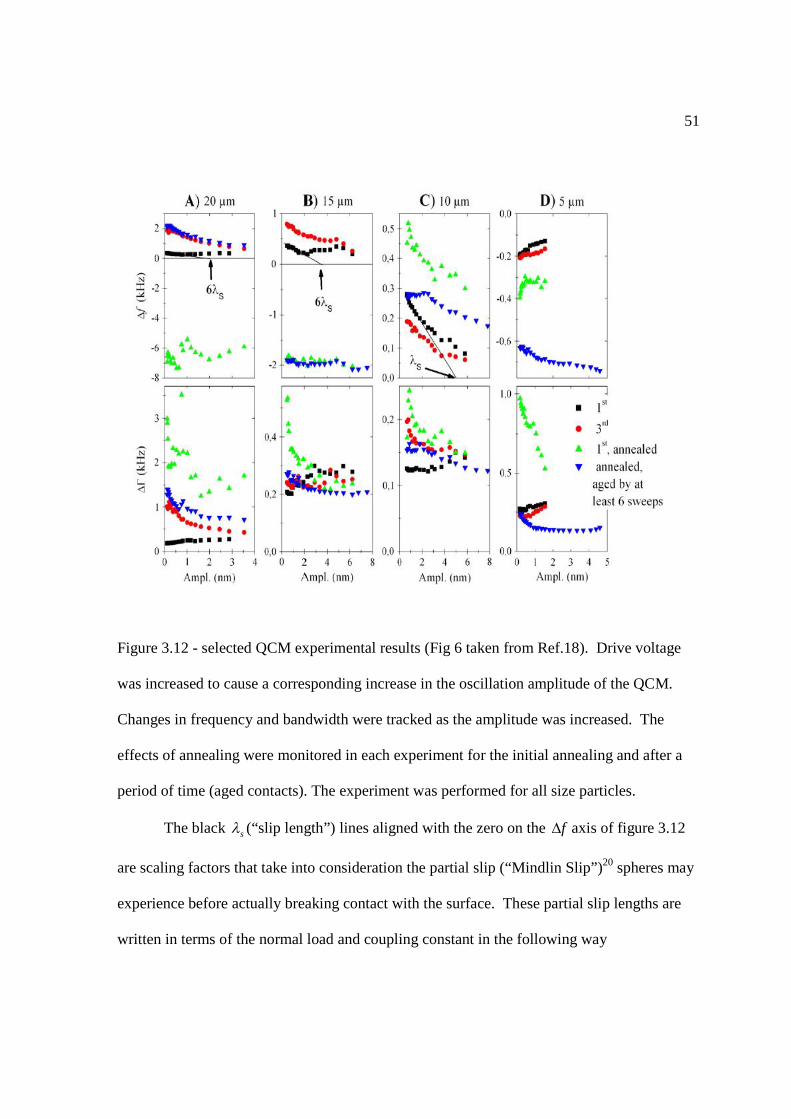
51

Figure 3.12 - selected QCM experimental results (Fig 6 taken from Ref.18). Drive voltage

was increased to cause a corresponding increase in the oscillation amplitude of the QCM.

Changes in frequency and bandwidth were tracked as the amplitude was increased. The

effects of annealing were monitored in each experiment for the initial annealing and after a

period of time (aged contacts). The experiment was performed for all size particles.

The black sl (“slip length”) lines aligned with the zero on the fD axis of figure 3.12

are scaling factors that take into consideration the partial slip (“Mindlin Slip”)20 spheres may

experience before actually breaking contact with the surface. These partial slip lengths are

written in terms of the normal load and coupling constant in the following way

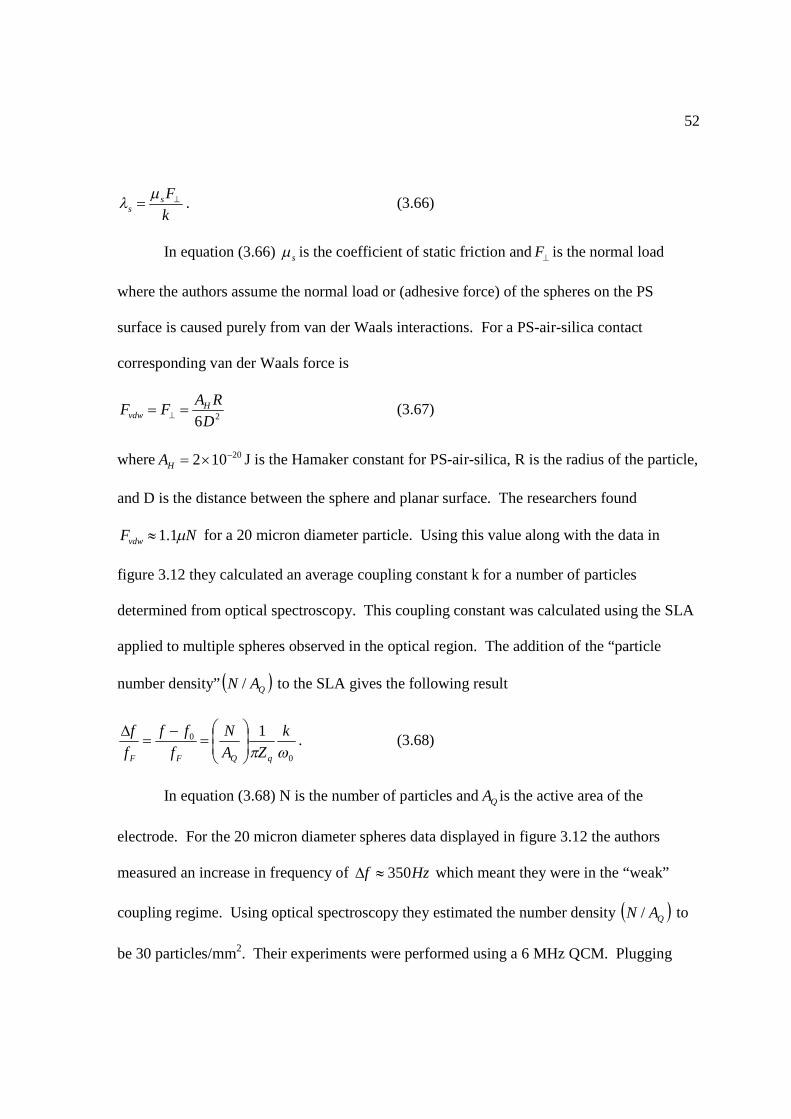
52

kFs

s^=

ml . (3.66)

In equation (3.66) sm is the coefficient of static friction and ^F is the normal load

where the authors assume the normal load or (adhesive force) of the spheres on the PS

surface is caused purely from van der Waals interactions. For a PS-air-silica contact

corresponding van der Waals force is

26DRA

FF Hvdw == ^ (3.67)

where 20102 -´=HA J is the Hamaker constant for PS-air-silica, R is the radius of the particle,

and D is the distance between the sphere and planar surface. The researchers found

NFvdw m1.1» for a 20 micron diameter particle. Using this value along with the data in

figure 3.12 they calculated an average coupling constant k for a number of particles

determined from optical spectroscopy. This coupling constant was calculated using the SLA

applied to multiple spheres observed in the optical region. The addition of the “particle

number density” ( )QAN / to the SLA gives the following result

0

0 1wpk

ZAN

fff

ff

qQFF÷÷ø

öççè

æ=

-=

D. (3.68)

In equation (3.68) N is the number of particles and QA is the active area of the

electrode. For the 20 micron diameter spheres data displayed in figure 3.12 the authors

measured an increase in frequency of Hzf 350»D which meant they were in the “weak”

coupling regime. Using optical spectroscopy they estimated the number density ( )QAN / to

be 30 particles/mm2. Their experiments were performed using a 6 MHz QCM. Plugging

53

these values into equation (3.68) gave what they considered to be an extremely high value for

the average coupling constant k which was equal to approximately 6000 N/m. They

compared this result to an analysis using Hertz theory.

aGk *= (3.69)

In equation (3.69) a is equal to the radius at the contact and *G is equal to the effective

modulus such that

÷÷ø

öççè

æ -+

-=

2

2

1

1*

22811

GGGnn

(3.70)

where 1 and 2 represent the PS layer and the glass (silica) sphere respectively. In equation

(3.70) G is a shear modulus and n is Poisson’s number. In equation (3.69) the contact radius

is found using Hertz theory (neglecting roughness and assuming semi-infinite substrate) and

is

3/1

* ÷øö

çèæ= ^

ERF

a . (3.71)

where

÷÷ø

öççè

æ -+

-=

2

22

1

21

*

11431

EEEnn

(3.72)

The reduced Youngs’ modulus is *E and the Youngs’ modulus is E. Since glass

spheres are much stiffer than the PS layer the terms 2E and 2G are approximately equal to

infinity. Using 3/11 »n the authors found a spring constant k=1000 N/m which is a factor of

6 smaller than their experimental value. The authors argue that discrepancies like the one

above from theory (Hertz) and experimental results have been observed in the past by other

54

and these high k values may be explained (qualitatively) by the existence of multi asperity

contacts.

3.8.1 - 20 MICRON SPHERE SUMMARY

Next the authors began with their interpretation of the results from figure 3.12. For

the 20 micrometer spheres they observed an initial increase in frequency after deposition.

After annealing the surface (increasing the contact area) they observed a decrease in

frequency below resonance which they explained as the system crossing over from the weak

coupling regime to the strong coupling regime in figure 3.9. Using the Sauerbrey equation

and comparing it to optical microscopy they found that 80% of the spheres must be “tightly”

bound to the surface. They however did mention that an alternate explanation was that the

system could reside in the intermediate range of figure 3.11 with k slightly above the

resonance value. The changed the surface properties by performing several (at least 6)

sweeps on the annealed sample. They found that the frequency of the system jumped up to

the starting values above resonance. They explained this by arguing the effects of annealing

where nullified by the contacts breaking during successive sweeps which lowered the mean k

value and brought the system back into the weak coupling regime.


Similar to the 20 micron spheres the authors observed an increase in frequency after

initial deposition. After annealing the surface they also observed a decrease in frequency

below resonance however, when they performed additional sweeps the frequency did not

jump back to the weak coupling regime (above resonance) as it did with the 20 micron

spheres in fact it did not change at all. They explained their results by stating that the

55

particles were so strongly attached to the surface that they did not decouple. They also

suggested that since the particles were smaller than the 20 micron particles moving them

would be more difficult because of the radial dependence of the peak force of the oscillation.

They applied the Sauerbrey equation to these particles and found that their result was off by a

factor of five. They attribute this error to the fact that the system for these size particles is in

the intermediate coupling range of figure 3.9 where analysis is extremely difficult.


When the particles where initially deposited and increase in frequency was observed

as with all previous cases. However, additionally runs after the deposition caused the

frequency to decrease (still above resonance) which is not in agreement with the previous

two particle sizes were the frequency further increased. After annealing the system

frequency increased above the values measured previous to the annealing. This result also

varied from the previous two cases where the frequency decreased upon annealing. The

authors explain this behavior by stating that the annealing process was not enough to move

the system into the strong coupling regime instead it only brought the mean k value closer to

the resonance condition which would explain the observed increase.


When these particles were deposited on the QCM a negative shift in frequency was

observed. The frequency did not change upon successive sweeps of the voltage. After

annealing the sample the frequency further decreased and after aging set in and more sweeps

were performed the frequency further decreased. The authors concluded that the spheres

were in the strong coupling regime.

56

The authors concluded by making some general statements about consistent behavior

found in all the experiments. One particular example was the bandwidth’s dependence on

QCM amplitude before and after the annealing process. Before annealing the authors found

that the bandwidth increased with the amplitude which is in agreement with their Mindlin

slip model (added dissipation from in place rocking). However, after annealing they

observed a decrease in bandwidth with increasing amplitude which is not an obvious result.

They argue that such a dependence could be explained by Coulomb friction. The authors do

however state that measurements of bandwidth alone are not sufficient to understand the

detailed mechanisms. The authors then briefly discuss optical data where surface damage

was observed after QCM experiments in the PS layer. They used these images to estimate a

particle velocity for the displaced sphere. They calculated the velocity in two different ways.

The first way took into consideration only one component ( xv ) of the velocity which yielded

a higher value then the second method that added a vertical component to their calculation.

In their concluding marks the authors summarized the results of their experiments by stating

that observed shifts in frequency are understood as a balance between the coupling and

inertial forces. Individual spheres have varying coupling constants (k) through out the active

region of the QCM. As a result measured coupling constants are interpreted as average

values over an approximate Gaussian distribution of spheres. A fully quantitative

determination of forces between the particles and QCM doesn’t seem possible since a

measured shift in frequency can be the result of varying coupling constants.

57

3.9 USING A QCM TO DETERMINE THE FRICTION LAW OF LOADING

PARTICLES

In 1993 researchers Sokoloff, Krim, and Widom pioneered a method21 for determining the

frictional force law of strongly coupled atomistic thin films on the surface of a QCM. The

astonishing thing about this method is that it is independent of the samples actual friction

law. This at first seems contradictory because in section 3.2 I discussed how a QCM probes

“viscous” friction or friction that obeys Stoke’s law

1vFf h-=. (3.73)

Where fF is the force of friction, h is the drag or “viscous” coefficient, and v is the

velocity. This apparent contradiction is removed when using a more general frictional force

law

)sgn(vvFn

f h-= (3.74)

where nn

vvv 12 -= is the magnitude of the relative velocity between the QCM velocity

( )tvv wcos01 = (3.75)

(the term 0v is the magnitude of the QCM velocity and w resonant angular frequency of the

QCM) and the strongly coupled slipping particles 2v . To account for the oscillating substrate

of a QCM the term sgn(v) is added on to account for the constant sign change of the force.

The term of interest in equation (3.74) is the power law n. The value of n determines the

type of frictional force the adsorbed particles experience while slipping on the surface.

58

Displayed below are figures which show the dependence of frictional force to velocity for

varying friction laws.

Ffriction

velocity

Coulomb0=n

1<n

1>n

1=n

Granular particles (Mindlin slip)

Viscous Frictiont

Amplitude

1<n

1>n

1=n

For strongly bound particles

Granular particles (Mindlin slip)

Viscous Friction

Coulomb

0=n

(a) (b)

Figure 3.13 – 3.13a shows the velocity dependence of various frictional force laws (n). 3.13b shows the QCM amplitude (velocity) dependence of the slip times (calculated using n=1) of adsorbed particles (strongly coupled regime) on a QCM.

The slipping velocity of the adsorbed particles 2v can be solved for exactly for the n=1 case

of viscous friction. This is achieved by first rewriting (3.74) as

)cos(022 tvm

vm

v whh=+&

(3.76)

where m is the mass of the adsorbed particles. Equation (3.76) is a first order differential

equation and is solved by multiplying both sides by the “integrating factor” t

meh

and

integrating. Applying this to equation (3.76) gives

dttem

vev

tm

tm )cos(0

2 wh hh

ò=. (3.77)

Using integration by parts twice on the right hand side of (3.77) allows one to solve for the

velocity which is

59

[ ])sin()cos()( 0021222

2 tmvtvmv wwhwhhw ++= -

. (3.78)

Using the result found from (3.78) along with the relation

( )tAv ww cos1 -= (3.79)

where A is the amplitude of particle slippage, the relative slipping distance of the particles

can be computed. Now returning to the original discussion, I stated earlier that the quantity

of interest in our friction analysis is n, so the question that remains is how the QCM is used

to measure this quantity. The methods discussed earlier in section 3.2 developed by Krim

and Widom that particle slip times can be calculated from the shifts in QCM frequency

fD (3.20) and shifts in inverse quality factor )/1( QD (3.19). The experiments reported in

this thesis use (3.20) to compute slip time values. A main result of the Sokoloff et. al

article21 was the dependence of the inverse quality factor to the amplitude

)11(1 nAQ--- » . (3.80)

Using (3.19) and (3.80) the particle slip time can be written in terms of the oscillation

amplitude and force law “n”

)11(~ nA

--t . (3.81)

Using equation (3.81) the force law “n” can be determined fro m the slope of the line created

from a log-log plot ( )ln(t vs. )ln(A ).

60

3.10 SLIDING FRICTION AND VELOCITY DEPENDENCE

As discussed in sections 3.2 and 3.10 a QCM can be used to probe sliding friction or to be

more specific, systems that follow Stoke’s law (3.73). In the previous section it was shown

how a QCM could be used to probe a wide variety of friction laws using Stoke’s law as a

baseline. These friction laws are velocity dependent and can be interpreted in the same way

as setting an object (the block shown in figure 3.14) at an initial velocity 0v and observing

the amount of time it takes for it to come to a complete stop.

substrate

Initial velocity relative to substratev0

Frictional Forcen

f vF h=

Figure 3.14 An illustration of an object set at an initial speed that is subject to a constant resistive damping force of friction that is velocity dependent. The object shown in this figure will eventually reach a final velocity of zero as a result of the damping force. The amount of time the object takes to reach this terminal velocity is dependent on the damping coefficient and the power law “n” of the damping force. In order to visualize the time it takes for an object to reach its terminal velocity on a QCM I

have created a theoretical plot (figure 3.16) that shows the decay of a particle’s initial

velocity over a period of time with the particle experiencing various velocity dependent

damping forces. The plot shown in figure 3.16 was constructed by first finding the

expression of the particle velocity as a function of time and then computing the characteristic

slip time of a particle as derived using Stoke’s law as a base line. In mathematical terms the

velocity as a function of time or )(tv was found by solving the following equation

61

vmFf &= (3.82)

where

nf vF µ . (3.83)

For the vast majority of “n” values equation (3.82) was in the form of a Bernoulli equation

(first order differential equation) and could be readily solved. Expressions for slip time were

computed using the following equation

0*tan vm

vtconsF nf t

-=-= . (3.84)

Results for a few sample values of n are displayed below in table 3.1.

Table 3.1 velocity and slip time values for various friction laws.

)(tvn t

21

-

1

2

0 tmF

vtv Nm-= 0)(

( )tmbevtv /0)( -=

tm

cvv

tv0

0

1)(

+=

3/22/3

0 23

)( ÷øö

çèæ -= t

md

vtv

NFmvm

t 0=

bm

=t

0cvm

=t

2/30v

dm

=t

The slip time shown for the n=1 case or “Stoke’s law” is independent of velocity which supports what was shown earlier in figure 3.13b. Table 3.1 along with additional values for n

62

were used to create the graph shown below in figure 3.15.

0.0 0.2 0.4 0.6 0.8 1.0 1.2 1.4 1.6 1.8 2.00.0

0.2

0.4

0.6

0.8

1.0

n=0 n=1 n=2 n= -0.5 n= -1 n=-2 n=100

v/v 0

t/t

MindlinRegime

Newton’sLaw

Stoke’sLaw

Coulomb’s Law

Figure 3.15 terminal velocity as a function of slip time for various friction laws. Values of n above 1 in figure 3.15 are representative in granular systems are known to follow

“Mindlin” friction behavior. The value of n=2 is known as Newton’s law of friction, where

as stated earlier n=1 is Stoke’s law and n=0 is Coulomb’s or Amonton’s law of friction.

From figure 3.15 it is shown that a system under going Coulomb friction reaches terminal

velocity in a period of exactly one slip time. For negative values of n terminal velocity is

reached before a complete slip time increment is reached. When n is larger than 0 terminal

velocities are reached at values above a single slip time.

63

3.10 REFERENCES

1. Vogt, B. D.; Lin, E. K.; Wu, W.-l.; White, C. C., Effect of Film Thickness on the Validity of the Sauerbrey Equation for Hydrated Polyelectrolyte Films. The Journal of Physical Chemistry B 2004, 108 (34), 12685-12690. 2. White, F. M., Viscous Fluid Flow. McGraw-Hill New York, 1974. 3. Widom, A.; Krim, J., Q factors of quartz oscillator modes as a probe of submonolayer-film dynamics. Physical Review B 1986, 34 (2), 1403-1403. 4. Johannsmann, D., Viscoelastic, mechanical, and dielectric measurements on complex samples with the quartz crystal microbalance. Physical Chemistry Chemical Physics 2008, 10 (31), 4516-4516. 5. Stockbridge, C. D., Vacuum Microbalance Techniques. Plenum: New York, 1966; Vol. 5. 6. Dybwad, G. L., A sensitive new method for the determination of adhesive bonding between a particle and a substrate. Journal of Applied Physics 1985, 58 (7), 2789-2789. 7. Martin, S. J.; Frye, G. C.; Ricco, A. J.; Senturia, S. D., Effect of surface roughness on the response of thickness-shear mode resonators in liquids. Analytical Chemistry 1993, 65 (20), 2910-2922. 8. Seah, P. J. C. a. M. P., The quartz crystal microbalance; radial/polar dependence of mass sensitivity both on and off the electrodes. Measurement Science and Technology 1990, 1 (7), 544-555. 9. Ballato, A., FREQUENCY-TEMPERATURE-LOAD CAPACITANCE BEHAVIOR OF RESONATORS FOR TCXO APPLICATION. IEEE Transactions on Sonics and Ultrasonics 1978, SU-25 (4), 185-191 10. Martin, S. J.; Granstaff, V. E.; Frye, G. C., Characterization of a quartz crystal microbalance with simultaneous mass and liquid loading. Analytical Chemistry 1991, 63 (20), 2272-2281. 11. Kanazawa, K. K.; Gordon, J. G., Frequency of a quartz microbalance in contact with liquid. Analytical Chemistry 1985, 57 (8), 1770-1771. 12. Flanigan, C. M.; Desai, M.; Shull, K. R., Contact Mechanics Studies with the Quartz Crystal Microbalance. Langmuir 2000, 16 (25), 9825-9829.

64

13. Johnson, K. L.; Kendall, K.; Roberts, A. D., Surface Energy and the Contact of Elastic Solids. Proceedings of the Royal Society of London. A. Mathematical and Physical Sciences 1971, 324 (1558), 301-313. 14. Lin, Z.; Hill, R. M.; Davis, H. T.; Ward, M. D., Determination of Wetting Velocities of Surfactant Superspreaders with the Quartz Crystal Microbalance. Langmuir 1994, 10 (11), 4060-4068. 15. Laschitsch, A.; Johannsmann, D., High frequency tribological investigations on quartz resonator surfaces. Journal of Applied Physics 1999, 85 (7), 3759-3759. 16. D'Amour, J. N.; Stålgren, J. J. R.; Kanazawa, K. K.; Frank, C. W.; Rodahl, M.; Johannsmann, D., Capillary Aging of the Contacts between Glass Spheres and a Quartz Resonator Surface. Physical Review Letters 2006, 96 (5), 058301-058301. 17. Borovsky, B.; Krim, J.; Syed Asif, S. A.; Wahl, K. J., Measuring nanomechanical properties of a dynamic contact using an indenter probe and quartz crystal microbalance. Journal of Applied Physics 2001, 90 (12), 6391-6391. 18. Vittorias, E.; Kappl, M.; Butt, H.-J.; Johannsmann, D., Studying mechanical microcontacts of fine particles with the quartz crystal microbalance. Powder Technology 2010, 203 (3), 489-502. 19. Dultsev, F. N.; Ostanin, V. P.; Klenerman, D., “Hearing” Bond Breakage. Measurement of Bond Rupture Forces Using a Quartz Crystal Microbalance. Langmuir 2000, 16 (11), 5036-5040. 20. Deresiewicz, R. D. M. a. H., Elastic spheres in contact under varying oblique forces. Journal of Applied Mechanics 1953, 20, 327-344. 21. Sokoloff, J. B.; Krim, J.; Widom, A., Determination of an atomic-scale frictional force law through quartz-crystal microbalance measurements. Physical Review B 1993, 48 (12), 9134-9134.

65

CHAPTER 4 - SPHERE ON FLAT CONTACT MECHANICS

4.1 INTRODUCTION

Understanding the fundamental nature of a contact is essential for any tribological study.

The importance only increases as one enters the microscale, where the force of friction

becomes extremely sensitive to both the nature of the contact and the area of contact. An

essential geometry characteristic for the topic of this thesis is the analysis of a sphere

interacting with a flat surface. This chapter will cover this geometry for both dry and humid

(wet) environments.

4.2 DRY CONTACTS

Simply put, a dry contact is one in which the contact behavior or adhesion between the

adjoining surfaces is purely dependent on the surface energies and loading forces of the two

contacts in the absence of external influences such as capillaries forming at the rim of the

contact as a result of a humid environment.

4.2.1 HERTZIAN CONTACT

One of the most basic and useful approximations for the contact area between a

sphere and flat geometry was worked out by Hertz1 in 1882. This geometry is displayed

below in figure 1 where the contact radius, radius of the particle, and the distance resulting

from elastic deformation is represented as a, R and z respectively. The Hertz model is used

66

to describe an elastic contact with the surface which suggests that the process of loading and

unloading is a reversible process. The contact radius a Hertzian Contact predicts is

3/1

43

÷÷ø

öççè

æ=

cERL

a (4.1)

where2

22

1

22 111

EEEc

nu -+

-= is the elastic modulus of the two surfaces in contact, R is the radius

of the sphere and L is the applied load. The “real” contact area associated with this contact

geometry is

3/2

2

43

÷÷ø

öççè

æ==

cERL

aA pp (4.2)

If the loading force is known, then the pressure associated from a Hertzean contact can be

calculated by dividing the loading force by (4.2)

3/13/2

341

LRE

P cm ÷

øö

çèæ=

p (4.3)

Equation (4.3) is an expression for the average (mean) pressure exerted at the contact area

however the pressure is not uniform though out. The pressure distribution is given by

2/12

0 1ïþ

ïýü

ïî

ïíì

÷øö

çèæ-=

ar

pp (4.4)

The deformation distance associated with a Hertzean contact is

3/1

2

22

169

÷÷ø

öççè

æ==D

cREL

Ra

z (4.5)

67

Figure 4.1 - Sphere flat geometry under elastic Hertzean contact. The Herzian model is a first approach to estimating contact area, but does not incorporate the

impact of adhesive forces on the size of the contact area.

4.2.3 THE DERJAGUIN APPROXIMATION

The Derjaguin approximation2 is an extension of the Hertzian contact model that

takes into account the effects of adhesive forces. It relates the force of adhesion adhF (the

main quantity of interest) between contacting surfaces to the interaction energy ( )DW

associated with their bond. This useful approximation is based on the assumption that the

radius of curvature between the two surfaces in contact is much greater than the separation

distance D and the range at which the adhesive force acts. This assumption is generally

applicable for the QCM experiments described in this thesis. The sphere on flat geometry,

which is of great importance for this thesis, is derived from an expression for the force of

adhesion between two contacting spheres given by3

)(2)(21

21 DWRR

RRDF spheresphere ÷÷

ø

öççè

æ+

=- p (4.6)

68

where 1R , 2R , and ( )DW are the radius of curvature for the first sphere, radius of curvature

for the second sphere, and the interaction energy per unit area as a function of separation

distance D respectively. Equation (4.6) has relevance for the conditions in our experiments,

in particular when microspheres adsorbed on the surface of our QCM are in direct contact

and/or on top of each other. The sphere on flat geometry is the special case of equation (6)

where RR =1 (the radius of the sphere) and ¥=2R (the flat or in our case QCM electrode).

Substituting these conditions into (4.6), one obtains:

)(2)( DRWDF flatsphere p=- . (4.7)

When surfaces come in contact with each other, the force of adhesion between them

is thus dependent on the corresponding surface energies between the interacting objects

(sphere and flat). The interaction energy ( )DW is generally expressed as the surface

energy sg which is an intrinsic property dependent on the materials intermolecular actions.

When the sphere and flat are made from the same material )2)(( 1221 ss DW gggg =Þ==

equation (4.7) reduces to

sadh RF gp4= (4.8)

Whenever the surfaces are comprised of different materials, ( )21 gg ¹ , then the

combined surface energy sg is approximated using the Good-Girifalco method4

212 ggfg =s (4.9)

The term f is a correction factor usually in the range5 of 0.5 to 1 to account for a the

varying intermolecular interactions.

69

4.2.2 JKR MODEL

The Johnson–Kendall-Roberts1 or (JKR) is an extension of the Hertz contact

geometry described in section 4.2.1. In the Hertz model the contact between the two surfaces

was assumed to be an elastic interaction with no energy lost from forming the contact. The

JKR model takes into consideration inelastic (irreversible) interactions between the contact

resulting from surface energy induced adhesive forces. The Hertz contact model only takes

into consideration the compressive loads associated with elastic contact which in most real

situation underestimates the real area of contact “a” shown in figure 1. To the Hertz pressure

distribution (4.4) the JKR model adds an additional “tensile” term to the Hertz pressure that

is compressive in nature. Equation (4.4) becomes

2/1

2

22/1

2

2

0 11)(-

÷÷ø

öççè

æ-¢+÷÷

ø

öççè

æ-=

ar

par

prp o (4.10)

where 0p¢ is negative and represents the tensile stress component that is induced from the

sphere adhering to the flat from surface energy. The form of equation (4.10) suggests that

the closer r is to the center, the contribution is mainly a result of compression. However, as r

moves closer to the edge of the contact, the pressure contribution is mainly tensile as

indicated by ( )rp diverging when ar = . This divergence occurs because the JKR model

assumes that the adhesion forces only act over the exact region in which contact is made.

This is an artificial condition. The divergence can be removed6 by substituting a real surface

interaction such as Van der Waals in place of the artificial condition. The increased tensile

energy causes the loaded sphere to elastically deform which causes the contact radius (a) to

increase beyond the value predicted by the Hertz model ( Ha ). The JKR model includes a

70

contribution of a possible external loading force in addition to the load present from the

surface energies ( 12W ) of the contacting objects (adhesion). The relationship between the

contact radius and load is

312

23

83

4aEW

RaE

F cc

ext p=÷÷ø

öççè

æ- (4.11)

where extF is the external loading force, a is the contact radius, 12W is the adhesion energy

between the two surface, and cE is the composite elastic modulus associated with the loading

(deformed) sphere. When no external load ( 0=extF ) is present the contact radius under JKR

theory becomes a constant value 0a that has the form

.9

3/1212

0 ÷÷ø

öççè

æ=

cERW

ap

(4.12)

In the presence of a loading force solving (4.11) for the contact radius gives

( ) ÷øöç

èæ +++= 2

1212123 363

43

RWFRWRWFER

a extextc

ppp . (4.13)

The JKR model can be used to predict an adhesion force in the absence of an external load.

This is done by equating the negative external loading force or “pull off force” to the elastic

restoring force of the sphere at the point of separation this is adhesion force is

RWFadh 1223 p= (4.14)

The contact radius at separation sa predicted by JKR is

3/10

4a

as = . (4.15)

71

The JKR model assumes perfectly smooth surfaces, which is clearly not the case for many

applications. However, this model does prove useful for materials such as rubber5 with low

elastic modulus where the rough contacting asperities flatten out at the contact.

4.3 CONTACT MECHANICS IN WET ENVIRONMENTS

In many experimental situations (such as the experiments examined in this thesis) the

JKR model can not be readily applied since the contacting asperities do not necessarily

flatten out from adhesive forces to form a perfectly smooth surface. When contacts are

unable to flatten out, separation gaps are present in between contacting asperities. These

gaps easily become filled with a mobile fluid (such as water) in the nearby vicinity. The

addition of this fluid has dramatic effects on the contact mechanics between interacting

surfaces. Since the experiments performed in this thesis compare humid and dry conditions,

we also examine the effect water has on the nature of the contact between the sphere and flat

geometry.

4.3.1 CAPILLARY PRESSURE

The capillary pressure Pcap originally derived by Young and Laplace7 in 1805

provides an expression for computing the pressure difference between arbitrary curved

surfaces that are present when liquids such as water attempt minimize surface energy by

forming a sphere.

÷÷ø

öççè

æ+=

21

11rr

P lcap g (4.16)

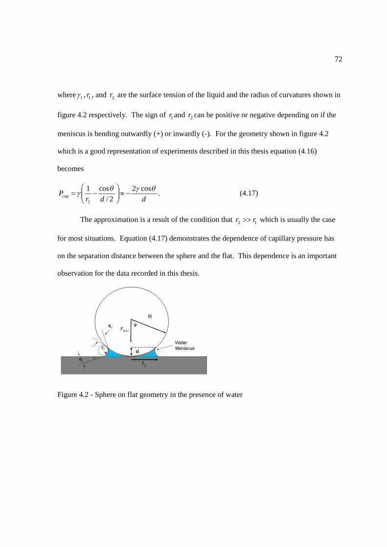
72

where lg , 1r , and 2r are the surface tension of the liquid and the radius of curvatures shown in

figure 4.2 respectively. The sign of 1r and 2r can be positive or negative depending on if the

meniscus is bending outwardly (+) or inwardly (-). For the geometry shown in figure 4.2

which is a good representation of experiments described in this thesis equation (4.16)

becomes

ddrPcap

qgqg cos22/

cos1

2

-»÷÷ø

öççè

æ-= . (4.17)

The approximation is a result of the condition that 12 rr >> which is usually the case

for most situations. Equation (4.17) demonstrates the dependence of capillary pressure has

on the separation distance between the sphere and the flat. This dependence is an important

observation for the data recorded in this thesis.

Figure 4.2 - Sphere on flat geometry in the presence of water

73

4.3.2 CAPILLARY CONDENSATION AND FORCES

Figure 4.3 - Zoomed in image of a microsphere and QCM surface in contact at varying levels of humidity.

Figure 4.3 is a visual interpretation of how capillaries from water vapor may be

distributed within the contact region of a sphere flat geometry. Since vapor pressure is

curvature dependent, it is possible for water vapor to condense at these asperity contacts at

lower vapor pressures then what is expected normally. This is the scenario illustrated from

(a) to (b) where (a) is a perfectly dry contact and (b) represents early water condensation. As

the humidity increases so does the amount of water trapped in the contacts (b). At some

point of extremely high humidity the contacts become completely filled as illustrated in (d).

The force of adhesion as a result of the presence of capillaries is a sum5 of the tensile and

compressive components of associated with the formation of a meniscus.

captenmen FFF += (4.18)

where menF , tenF , and capF are the meniscus force, tensile of “tension” component of force, and

the “compressive” force normal to the surface capillary. In most cases the tensile component

74

is much smaller than the contribution from the capillary interaction thus capmen FF » . The

capillary force is directly proportional to the capillary pressure (4.17) such that

APF capcap ´= where A is area of the meniscus parallel to the surface. For cases where

j (figure 4.2) is small and the water wets both surfaces, the meniscus force becomes

ladhmen RFF gp4»= . (4.19)

This equation has the same form as equation (4.8) which approximated the adhesion force for

a dry contact.

75

4.4 REFERENCES

1. Johnson, K. L.; Kendall, K.; Roberts, A. D., Surface Energy and the Contact of Elastic Solids. Proceedings of the Royal Society of London. A. Mathematical and Physical Sciences 1971, 324 (1558), 301-313. 2. Derjaguin, B., Untersuchungen über die Reibung und Adhäsion, IV - Theorie des Anhaftens kleiner

Teilchen. Kolloid-Zeitschrift 1934, 69 (2), 155-164. 3. Israelachvili, J., Intermolecular and Surface Forces. Elsevier: (1985-2004); Vol. 2. 4. Girifalco, L. A. a. G., R. J., A theory for the estimation of surface and interfacial energies. . Journal of Physical Chemistry 1957, 64, 904-909. 5. Mate, C. M., Tribology on the small scale a bottom up approach to friction,lubrication, and wear. Oxford University Press: New York, 2008; Vol. 1, p 333. 6. Muller, V. M.; Derjaguin, B. V.; Toporov, Y. P., On two methods of calculation of the force of sticking of an elastic sphere to a rigid plane. Colloids and Surfaces 1983, 7 (3), 251-259. 7. Adamson, A. W. a. G., A.P., Physical Chemistry of Surfaces. Wiley: New York, 1997.

76

CHAPTER 5: FRICTION ANALYSIS OF 5 MICRON

POLYSTYRENE SPHERES DEPOSITED FROM AQUEOUS

SOLUTION ON A QUARTZ CRYSTAL MICROBALANCE

I. Lynch, J. McNutt*, and J. Krim

Department of Physics North Carolina State University

*Department of Physics University North Carolina Asheville

In this study we have employed a Quartz Crystal Microbalance (QCM) in conjunction

with optical techniques to analyze the frictions and adhesion of 5µm diameter polystyrene

spheres physisorbed on an oscillating QCM electrode. Upon placing the particles on the

surface, we observe a negative shift in frequency, indicating that the particles are in a strong

coupling regime of adhesion1. In this regime, the Sauerbrey equation should be sufficient to

estimate the mass loading of the microspheres. An optical count of the microspheres on the

electrode confirmed this assumption, if corrections for slipping are taken into account.

Optical observations also reveal that the particle motion depends on the oscillation direction

and surface topology of the QCM. To explore the nature of the decoupling (small amplitude

in-place oscillatory motion, rupture and reattachment, rupture and complete particle removal,

etc) the QCM frequency response was monitored while the drive level was increased and

decreased. The resulting “decoupling curve” is reflective of the nature of the particle

adhesion to the QCM surface as well as the friction law governing it. For the case of

particles “slipping in place” it is possible to calculate an average slip time τ associated with

the QCMs frequency response to the effective decrease in massloading. We found that the

slip time values are of the same order as slip times previously recorded in the literature 2 for

77

physisorbed sytems, including water. After an initial drying and run-in period, the particles

exhibit frictional behavior that is nearly independent of vibrational amplitude, as would be

the case for a system strictly governed by a viscous friction law. The behavior may arise

from the presence of physisorbed water at the interface, which is ubiquitous in air.

5.1 INTRODUCTION

The notion of transporting micro/nano objects has been of interest to the scientific

community since the early days of nanotechnology. Progress in this area requires an

understanding of the frictional behavior of these objects when they are in motion. Transport

and manipulation of nano and micro devices is a necessary application of both nano/micro

technology that is as intriguing as it is complex. Obtaining this control can lead to many

exciting advancements that span from drug delivery in nanobiotechnology3, micro particle

sorting and grouping by mass4, particle monitoring for toxicological studies as well and many

more favorable applications that span multiple disciplines. However, before these

applications can become a reality several questions must be addressed. What forces

contribute to the friction between the device and surface? How strong are these forces? Can

they be manipulated and if so how? At the micro/nano scale it has been observed in the

literature 5 that particle dynamics are dramatically different than what is seen for the macro

or meso length scales. This is due to the fact that intermolecular and capillary forces become

increasingly important at these length scales.

We focus here on polystyrene microspheres, which are of growing interest due to

their medical and textile applications. In particular microencapsulation of phase change

materials (PCMs) using polystyrene microspheres, has potential applications toward medical

78

hot/cold therapy as well as manufacturing clothing to handle extreme weather conditions.6

Dultsev and coworkers, in a pioneering 2000 publication 4, suggested that quartz crystal

microbalances (QCM’s) could have wide spread potential applications for separation, sorting,

and sizing. In their experiment polystyrene microspheres were attached to the oscillating

surface of a QCM by multiple interactions and detachment of the spheres from the QCM was

achieved by varying the driving voltage of the QCM. The sample was oriented horizontally

with the spheres deposited on the top side of the electrode. The detachment was inferred by

measuring the “sound” the spheres emit upon detaching with respect to the voltage at which

the crystal was being driven.

The experimenters also measured the change in the resonant frequency of the QCM

as a function of the driving voltage. They attributed the changes in frequency of the QCM to

be a result of the spheres detaching from the surface and eventually rolling off the edge of the

QCM causing the mass to decrease which results in a frequency change in the QCM. This

explanation is theoretically sound however, a similar shift in frequency can be observed

when a portion of spheres no longer track the motion of the resonator as a result of surface

decoupling from slipping, sliding, and/or rocking in place in a bound region.

Sokoloff7 explored this possibility, by theoretically examining the form of a QCM response

to sliding adsorbed layers whose friction laws were of the form:

vm

F filmfriction

rr

t-= n (5.1)

where mfilm is the mass of the film, v is the sliding velocity, and t is a slip time characteristic

of the particle-substrate friction2. For the case of tightly bound films, Sokoloff reported that

79

slip time measurements recorded as a function of the amplitude of vibration of the QCM

would reveal the form of the friction law, according to:

)/11(1)( nAQ --- »µ¶ t (5.2)

We report here measurements of sliding friction analysis, and images to document the

nature of decoupling observed. In our experiment the particles in our optical region did not

roll off the surface. However, for a small percentage of the particles in the optical region

motion was observed. The observed motion was dependent on the oscillation direction and

surface topology of the QCM. Before we address the details of our experiment we will begin

with a review of prior work outlining QCM response due to various load configurations.

We found that the slip time values are of the same order as slip times previously

recorded in the literature 2 for physisorbed sytems, including water. After an initial drying

and run-in period, the particles exhibit frictional behavior that is nearly independent of

vibrational amplitude, as would be the case for a system strictly governed by a viscous

friction law. The behavior may arise from the presence of physisorbed water at the interface,

which is ubiquitous in air.

5.2 QCM RESPONSE TO LOAD CONFIGURATION AND BEHAVIOR

In what follows we will discuss the results of previous QCM experiments in which

depending on the nature of the experiment, the QCM experiences a shift either in the positive

or negative direction from natural resonance. First we will discuss is the Sauerbrey case

which deals with molecularly thin films that are rigidly attached to the QCM (figure 1a). In

1959 Sauerbrey 8 showed that the mass absorbed on the electrode of a QCM is directly

proportional to the measured frequency shift (5.3).

80

20

)/(2 f

v

Amf

qq

filmfilm r

d -= (5.3)

where mfilm is the mass of a loading film rigidly attached to the motion of the QCM, A is the

area of the electrode, ρq is the density of quartz, νq is the velocity of sound through quartz,

and 0f is the resonant frequency of the QCM. This equation corresponds to negative shifts in

frequency and works well when the loading mass is rigidly attached to the QCM’s motion.

Next we will discuss what we denote as the Krim et. al. case9. This case describes the

frequency response of a QCM coated with a molecularly thin film whose bond with the

surface is strong, but not completely attached to the QCM’s motion as a result of surface

slippage (figure 5.1b). The sliding film is assumed to obey the viscous friction law which

means the force of friction is velocity dependent (no static friction) as shown in the following

equation.

vm

F filmfriction

rr

t-= (5.4)

In this equationt represents the slip time of the film which by definition is the time it takes

for the film sliding velocity to diminish to 1/e of its original value and vr

represents the

average film sliding speed. The frequency response to this type of behavior is described by

equation (5.5) below

2)(1 wtd

d+

= filmmeasured

ff (5.5)

where w is the angular resonant frequency of the crystal. When there is no film slippage

( 0=t ) (5.3) reduces to (5.1). The Krim et. al. case along with the previously mentioned

Sauerbrey case result in a negative shift from resonance of the unloaded QCM frequency.

81

The difference is that the shift for the Krim et. al. case is smaller by a factor of ( )21

1

wt+

which is shown in (5.5). The next case we will discuss (figure 5.1c) gives rise to a positive

shift in QCM frequency, this is the Dybwad case10. In this experiment large (compared to the

two previous cases which were on atomistic length scales) spherical gold particle between

10-50 mm were loosely attached to the surface of a QCM and the resulting frequency shift

from resonance was positive. Dybwad constructed a coupled oscillator model that accurately

predicted the observed behavior. This model has since been modified by the addition of a

complex spring constant to extract additional information concerning the added dissipation to

the QCM upon interaction with surface particles1, 11. According to the Dybwad model a

QCM’s frequency shift is dependent on the bond strength between the load particle(s) and

QCM surface. It is difficult to employ the Dybwad model to predict the response of a QCM

as a result of bond strength when the data lies near the transition from positive to negative

shifts12.

The next case which we denote as the Laschitsch and Johannsmann/Borovsky et. al.

case13 (figure 1d) deals with the QCM’s response to point or “asperity” contacts. To simulate

this geometry they pressed a probe tip into the surface of the QCM, which resulted in an

increase in the QCM’s frequency proportional to the contact area between the tip and

electrode surface. This increase was interpreted as an added stiffness to the QCM resulting

from spherical waves emitted from the probe point contact. The observation of a positive

frequency shift is not limited the single sphere geometry of the Dybwad experiment nor the

82

previously mentioned probe tip geometry but, can easily be realized using sub-monolayer

and monolayer coverages.

For example, in an experiment performed to study the effects of capillary adhesion to

glass microspheres (45-700 mm ) deposited on the surface of a QCM with a gold electrode11.

The researchers observed a positive shift from resonance when a monolayer of spheres was

deposited, that further increased once the bonds where tightened due to capillary forces

further stiffing the surface. This observation agrees with the combined results of the Dybwad

and the Laschitsch and Johannsmann/Borovsky et. al. cases. The last configuration we will

discuss is the Flanigan et. al. case (figure 5.1e) and it results in a negative shift in QCM

frequency. When a viscoelastic medium such as a gel cap is placed on the surface of a QCM

the resulting shift in frequency is negative.

In contrast to the previous case, Flanigan et al. found that by increasing the contact

area between the gel cap and QCM surface the frequency decreased approximately in direct

proportion14. Combining the Flanigan and Johannsmann/Borovsky et. al. cases gives

implications about the effect a melting surface would have on the frequency of a QCM.

Currently experiments15 are being conducted where an STM tip is in contact with an

oscillating QCM coated with a thin film. It has been shown15 that frictional heat generated

from the STM/QCM interaction can cause a detectable phase change in the thin film. This

phase change can be monitored by recording the changes in QCM frequency.

When the STM tip is initially in contact with the QCM the Laschitsch and

Johannsmann/Borovsky case applies and one observes a positive shift in frequency.

However, when the film undergoes a solid to liquid phase change the resulting shift in

83

frequency is negative and is best explained using the Flanigan et. al. case. In summary a

QCM experiences a negative shift from the Sauerbrey case which describes the affect a

rigidly attached film has on the natural frequency a QCM. The next case is the Krim et. al.

which results in a negative shift from resonance that is smaller then the shift from the

Sauerbrey case due to surface decoupling and slippage effects. We employ the latter

approach here to infer particle slip times, as we are able to infer mass loading from both an

optical count of the particles, and from the frequency shift associated with mass loading.

Figure 5.1 - Depiction of previously studied load geometries of QCM experiments.

5.3 EXPERIMENTAL SETUP

In our experiment we depositied a sub monolayer (1-10%) of polystyrene

microspherical particles on the top electrode of a QCM. We initially observed a negative

shift in resonant frequency which suggested that the particles where in the strong coupling

regime according to the small load approximation 16 and agreed with Sauerbrey’s prediction.

. We suspected that as a result of the oscillatory nature of the QCM it was possible that a

84

fraction of the spheres deposited on the surface could be loosely attached or “decoupled” and

as a result increase the initial negative frequency shift caused by the majority particles that

were rigidly attached to the surface. To test this we increased the drive voltage of our QCM

and recorded the frequency response against crystal amplitude. We then decreased the drive

voltage to its starting value to track the frequency response in both directions. We assigned

the name “decoupling curve” to this particular measurement. This type of measurement has

been performed before in the literature in the forward direction alone.4, 12We believed that by

steadily increasing the drive voltage of the QCM we would create more decoupling events

which would be sensed by the crystal and recorded as a relative increase in frequency. When

decreasing the drive voltage back to the original value we observed some interesting

hysteresis behavior. This hysteresis raised further questions about the actual dynamics and

behavior of the particles on the surface. Our main goal for this experiment was to obtain

information regarding the frictional force at this micron scale which is currently not well

understood11. Interestingly enough probing friction at the atomistic scale is a much easier

feat when implementing techniques developed by the Krim group9, 17. As mentioned in the

previous section when a thin uniform film deposited on the electrode of a QCM begins to slip

as a result of the oscillatory motion, frictional properties (in particular the slip time) can be

probed from changes in both the quality factor Q and resonate frequency of the QCM.

Current analytical models (Sauerbrey8, Kanazawa-Gordon18, and Krim group9, 17) describe

properties of uniformly distributed thin films on a QCM. However, our experiments do not

fit the conditions of these models. Spring models such as the Dybwad and

Johannsmann/Borovsky et. al. cases are the most appropriate to describe surface behavior in

85

our experiments. When analyzed with a spring interpretation decoupling curves in principle

describe changes in coupling and stiffness between the particles and surface as the amplitude

of oscillation is increased and then decreased to the original value. This information can be

used to infer surface dynamics as the amplitude of oscillation is swept forward and

backward. Since we are not aware of any existing model that can accurately describe

frictional behavior for our experimental configuration, we used the previously mentioned

methods developed by the Krim group that describes sliding molecularly thin films as our

baseline theory for this undeveloped configuration to calculate particle slip times during

initial deposition and the forward sweep of our decoupling curve. This method assumes that

the microspheres obey a velocity dependent friction law which may or may not be the case

for the microscale.

5.4 METHODS AND MATERIALS

Figure 5.2 - Sketch of experimental apparatus.

Our QCM’s (Laptech Precision, Inc.) were AT cut at 35˚ and the diameter was 0.375

inches with a 0.01 inch flat on the –x axis and were used directly out of the package. The

Oscillator Circuit

Sample

Microscope + CCD Camera

Frequency Counter + Multimeter

Computer

Power Supply 25 microns

25 microns

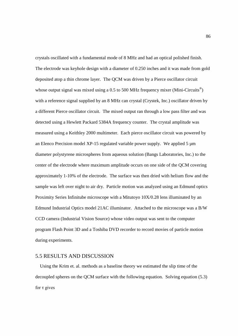
86

crystals oscillated with a fundamental mode of 8 MHz and had an optical polished finish.

The electrode was keyhole design with a diameter of 0.250 inches and it was made from gold

deposited atop a thin chrome layer. The QCM was driven by a Pierce oscillator circuit

whose output signal was mixed using a 0.5 to 500 MHz frequency mixer (Mini-Circuits®)

with a reference signal supplied by an 8 MHz can crystal (Crystek, Inc.) oscillator driven by

a different Pierce oscillator circuit. The mixed output ran through a low pass filter and was

detected using a Hewlett Packard 5384A frequency counter. The crystal amplitude was

measured using a Keithley 2000 multimeter. Each pierce oscillator circuit was powered by

an Elenco Precision model XP-15 regulated variable power supply. We applied 5 µm

diameter polystyrene microspheres from aqueous solution (Bangs Laboratories, Inc.) to the

center of the electrode where maximum amplitude occurs on one side of the QCM covering

approximately 1-10% of the electrode. The surface was then dried with helium flow and the

sample was left over night to air dry. Particle motion was analyzed using an Edmund optics

Proximity Series Infinitube microscope with a Mitutoyo 10X/0.28 lens illuminated by an

Edmund Industrial Optics model 21AC illuminator. Attached to the microscope was a B/W

CCD camera (Industrial Vision Source) whose video output was sent to the computer

program Flash Point 3D and a Toshiba DVD recorder to record movies of particle motion

during experiments.

5.5 RESULTS AND DISCUSSION

Using the Krim et. al. methods as a baseline theory we estimated the slip time of the

decoupled spheres on the QCM surface with the following equation. Solving equation (5.3)

for τ gives

87

11

-D

D=

film

gmassloadin

f

f

wt (5.4)

which shows that the slip time of the particles is proportional to the frequency shift of the

QCM due solely to particle loading. Here the frequency shift of the film represents the shift

in frequency from decoupled spheres when the amplitude of oscillation is increased. We

understood that it was possible that a fraction of spheres may have been decoupled during the

initial oscillation of the crystal which would lead to an underestimated value for the

frequency shift due to mass loading. To correct for this we scanned and imaged the entire

electrode surface and counted the individual spheres on each image. We took this value and

compared it to the amount of spheres predicted by applying the Sauerbrey equation from the

extended Dybwad model (for one side of the QCM) to our initial frequency shift. The

difference in these values corresponded to the amount of decoupled spheres. Applying the

Sauerbrey equation once more we calculated the amount of frequency shift the decoupled

spheres would cause if they were not decoupled. We then added this value to the initial

measured frequency shift to obtain an estimated value for the true mass loading frequency

shift. The modified Sauerbrey equation 1, 11 (equivalent to equation (5.1)) is written as

0fZm

Nfq

sgmassloadin p

w-=D (5.5)

where N is the number per unit area of microspheres, sm is the mass of a single microsphere,

126108.8 --´== skgmvZ qqq r is the impedance of quartz, and 02 fpw = is the angular

frequency of the unloaded QCM. On the electrode surface we counted a total of 6,353

spheres.

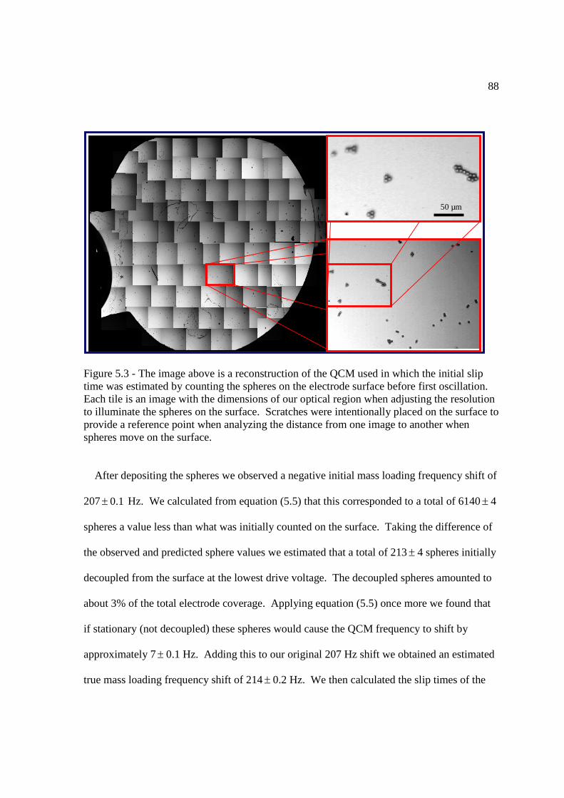
88

Figure 5.3 - The image above is a reconstruction of the QCM used in which the initial slip time was estimated by counting the spheres on the electrode surface before first oscillation. Each tile is an image with the dimensions of our optical region when adjusting the resolution to illuminate the spheres on the surface. Scratches were intentionally placed on the surface to provide a reference point when analyzing the distance from one image to another when spheres move on the surface.

After depositing the spheres we observed a negative initial mass loading frequency shift of

207 1.0± Hz. We calculated from equation (5.5) that this corresponded to a total of 6140 ± 4

spheres a value less than what was initially counted on the surface. Taking the difference of

the observed and predicted sphere values we estimated that a total of 213 ± 4 spheres initially

decoupled from the surface at the lowest drive voltage. The decoupled spheres amounted to

about 3% of the total electrode coverage. Applying equation (5.5) once more we found that

if stationary (not decoupled) these spheres would cause the QCM frequency to shift by

approximately 7 ± 0.1 Hz. Adding this to our original 207 Hz shift we obtained an estimated

true mass loading frequency shift of 214 ± 0.2 Hz. We then calculated the slip times of the

50 µm

89

decoupled particles by applying equation (5.4) to the forward sweep of the initial decoupling

curve using our corrected mass loading frequency shift as a baseline. Our results are

displayed in the following table.

Table 5.1 - Calculated slip times from forward decoupling curve run. Drive Voltage(V)

Crystal Amplitude (mV)

Frequency Shift of Film(Hz)

Slip Time (ns)

8.53 64.8 207 3.7 ± 0.06 9.58 74.9 199 5.5 ± 0.06 10.5 81.6 195 6.2 ± 0.07 11.57 89 186 7.7 ± 0.07 12.56 95.7 183 8.2 ± 0.07 13.53 100.9 179 8.8 ± 0.07 14.57 105.1 176 9.2 ± 0.07 15.57 108.1 170 10.1 ± 0.08

Given the slip times calculated in table 1 we were interested to see what the approximate

amplitude of sphere slippage was relative to the substrate. Keeping with our assumption of a

linear velocity dependent viscous friction law (5.2) we use the equation of motion derived by

Sokoloff et al 7 (5.6) of the velocity of a slipping film (in our case microspheres) as a

function of the relative velocity between the moving QCM substrate and slipping film.

)sgn( 12122 vvvvvm ---= g& (5.6)

Where tg /sm= is the damping coefficient from (5.2), 2v is the velocity of the slipping film,

and )cos(01 tvv w= is the velocity of the QCM at a given amplitude. Equation (5.6) can be

solved exactly for 2v

( )[ ])sin(cos)( 0021222

2 tmvtvmv wwgwggw ++= - . (5.7)

90

Using vector addition on 1v and equation (5.7) we solved for the relative velocity between

the sphere and substrate. From the angular frequency and the calculated relative velocity we

obtained results for the approximate relative amplitude of particle slippage as shown in figure

5.4.

0.0 2.0x10-7 4.0x10-7 6.0x10-7 8.0x10-7

-8.0x10-9-6.0x10-9-4.0x10-9-2.0x10-9

0.02.0x10-94.0x10-96.0x10-98.0x10-9

0.0 2.0x10-7 4.0x10-7 6.0x10-7 8.0x10-7

-4.0x10-10-3.0x10-10-2.0x10-10-1.0x10-10

0.01.0x10-102.0x10-103.0x10-104.0x10-10

maximum qcm drive voltage

Slip

Dis

tanc

e (m

)

Time (s) minimum qcm drive voltage

Slip

Dis

tanc

e (m

)

Time (s)

t=10.1 nsv

0=0.8 m/s

t=3.7 nsv

0=0.1 m/s

Figure 5.4 -Results above were calculated from the slip time values displayed in Table 5.1 for the initial (minimum) drive level and the final (maximum) drive level.

We assumed typical15 QCM velocities of 0.1 m/s and 0.8 m/s for the minimum and

maximum drive levels respectively. Figure 5.4 suggest that the surface particles slosh back

and forth at atomist dimensions for the weakest drive level displaying a relative amplitude

range an order of magnitude lower than the estimated 2 nm amplitude of vibration of the

QCM. At the strongest drive level the particles move at comparable distances with the

estimated amplitude of QCM vibration which was approximately 15nm for a substrate

velocity of 0.8 m/s.

91

Figure 5.5 - (a) in this figure represents an idealized depiction of the QCMs response to in place particle decoupling or “decoupling curve” in the strong coupling regime of the Dybwad model. The graph shows no hysteresis because it assumes that particles return to initial state once crystal amplitude decreases to original drive level. The graph to the right (b) is the actual experimental data that table 1 is based on.

From figure 5.5(b) it is evident that particles are in the strong coupling regime of Dybwad

model as shown by the initial negative shift in frequency from the null curve and the initial

decoupling curve (run 1 forward). As the crystal amplitude increased in run 1 we observed

(roughly) a linear increase in frequency which agreed with figure 5.5(a). However, when

decreasing the drive voltage back to the original level which in turn decreased the crystal

amplitude we observed hysteresis. This hysteresis indicates that even though these drive

levels were insufficient to eject particles from the surface or even cause noticeable motion in

the optical region changes in coupling deep within the buried contact between the

microspheres and the gold electrode were detected by the QCM. The increase in frequency

observed during the decreasing sweep of the decoupling curve in run 1 indicates that the

60 65 70 75 80 85 90 95 100 105 110 115

8005335

8005350

8005365

8005380

8005500

8005515

8005530

8005545

Fre

quen

cy (

Hz)

Amplitude (mV)

No Spheres on Surface Null_forward Null_backward

Spheres on surface run 1_forward run 1_backward run 2_forward

(b) (a)

92

average coupling of the spheres on the surface has decreased. In figure 5.6 the behavior

between runs 1 and 2 are magnified to show the difference in decoupling behavior. Initially

the slope in the increasing decoupling curve for run 2 is less than that for run 2 until some

critical amplitude around 105 mV is reached to further weaken even more bonds on the

surface as indicated by the sharp increase in slope shown in figure 5.6.

60 70 80 90 100 110 1208005325800533080053358005340800534580053508005355

80053608005365

8005370800537580053808005385

Fre

quen

cy (

Hz)

Amplitude (mV)

Spheres on Surface run 1_forward run 1_backward run 2_forward

Figure 5.6 - Magnification of runs 1 and 2 from figure 5.5(b)

93

Figure 5.7 - Friction analysis of Figure 5.6 decoupling curves. Figure 5.7 (a) is a plot of the change in frequency from QCM resonance plotted against the crystal amplitude. Run 2 in (a) has been divided into two regions to analyze the change in frictional behavior associated with the transition between regions. The values of n displayed in (b), (c), and (d) correspond with the particle friction law as shown in equation (5.1). These n values were calculated by applying equation (5.2).

Optical data was recorded for both the long and short run decoupling curves in the

horizontal orientation and we observed no gross movement of the surface particles when

viewing the center of the electrode where the QCM amplitude is a maximum. However, our

data suggest that the particles are not completely idle. The decoupling curve results from

figures 5.5 and 5.6 suggest that these particles are undergoing some sort of behavior

(rocking, sliding, slipping, reordering, depinning, etc…) that reduces the average coupling

4.1 4.2 4.3 4.4 4.5 4.6 4.7-19.6

-19.4

-19.2

-19.0

-18.8

-18.6

-18.4

ln(

slip

tim

e) (

s)

ln( Xtal Amplitude) (mV)

run 1_forward Linear Fit of ln( slip time)

n=0.36

Coulomb like friction

(b)

slope=1.8

4.35 4.40 4.45 4.50 4.55 4.60 4.65 4.70-18.32

-18.31

-18.30

-18.29

-18.28

-18.27

-18.26

ln(

slip

tim

e) (

s)


run 2_forward_region 1 Linear Fit of ln( slip time)

n=0.85

(c)

viscous like friction

slope=0.17

4.67 4.68 4.69 4.70 4.71 4.72 4.73-18.28

-18.26

-18.24

-18.22

-18.20

-18.18

-18.16

ln(

slip

tim

e) (

s)


run 2_forward_region 2 Linear Fit of ln( slip time)

n=0.36

(d)

Coulomb like friction

slope=1.8

60 70 80 90 100 110 120-210

-205

-200

-195

-190

-185

-180

-175

-170

-165

-160

-155

-150

Df

Xtal Amplitude (mV)

run 1_forward run 2_forward

region 1

region 2

(a)

94

between the particles and substrate. In figure 5.7 (a) we see that our frequency shift “Δf”

against crystal amplitude agrees with the trend one would expect to see for particles

undergoing Coulomb like friction as worked out by Vittorias et al.12 This result is favorable

since we observed no loss in particles but still saw an obvious shift in frequency. Using

methods developed by the Krim group we simplified the decoupling mechanism to be in

place slipping in which frictional results can be worked out. We found under this assumption

that our 5 micron diameter polystyrene microspheres adsorbed from aqueous solution behave

like ordinary physisorbed films previously studied in the literature.2

This observation was in the opposite direction of the initial shift observed by

D’Amour et. al in their study of capillary adhesion11 however, agreed with the experiment

performed by Dultsev and coworkers. The discrepancy may be a result of the differences in

the deposition as well as the size (ours were smaller) and/or composition (glass vs.

polystyrene) of the particles. D’Amour et. al found that particles with diameters smaller than

40µm did not agree with small load approximation theory for weak coupled particles 11

which is in agreement with the work presented here. In our experiment spheres were

deposited from aqueous solution where capillary bridges form between the spheres and QCM

surface, these bridges clamp the spheres in place allowing them to track the motion of the

QCM. In their experiment the spheres were deposited from a dry state where the rms

roughness of the spheres was an order of magnitude larger than their QCM surface 11 which

increases the possibility of point contacts upon deposition as well as the chance for their

experiment to fall into the weak coupling regime. In conclusion we found that when QCM

experiments (decoupling curves) were performed on our polystyrene particles experienced

95

initially a “Coulomb like” friction as they underwent some decoupling process that

effectively decreased the average adhesion to the surface. When decreasing the crystal

amplitude to the original value we observed hysteresis in frequency indicated by the

observed increase in frequency from the initial value before the experiment was performed.

This suggested that the overall coupling

strength of particles to the surface has decreased as a result of the initial sweep forward.

Figure 5.8 - Particle motion observed after rapidly varying the driving voltage. Figures (a) and (b) serve to illustrate a reordering mechanism that may occur during QCM experiments. These figures were performed on a different sample in which we observed top layer spheres transition to the surface of the QCM. This motion suggests the sphere-sphere bond is weaker than the spheres-electrode bond.

When performing the experiment a second time we found that the particles

experienced a viscous like friction law similar to that of a physisorbed monolayer until some

critical crystal amplitude value above what was previously tested was reached to induce

particle decoupling which placed particles in a Coulomb like friction regime identical in

value to what was observed initially. This suggest that the particles are essentially “picking

up where they left off” from the initial decoupling run. For a completely viscous friction law

we would expect to calculate a value of 1 for n however, as shown in figure 5.7(c) we

50 µm 50 µm

(a) (b)

t1 = 112s t2 = 114s

96

calculated n=0.87 which is viscous like but suggest other mechanisms are at work on the

surface that hinder a completely viscous friction law. These mechanisms as mentioned

earlier include decoupling, depinning, and reordering of the surface during the QCM

experiment. In figures 5.8 (a) and 5.8 (b) we show one possible reordering mechanism that

may contribute to moving the system away from a completely viscous friction law. Although

we did not observe any movement or behavior in the optical region it is not fair to assume

that all of the particles on the entire surface are experiencing the same inactivity.

97

5.6 REFERENCES

1. Johannsmann, D., Viscoelastic, mechanical, and dielectric measurements on complex samples with the quartz crystal microbalance. Physical Chemistry Chemical Physics 2008, 10 (31), 4516-4516. 2. Krim, J.; Watts, E. T.; Digel, J., Slippage of simple liquid films adsorbed on silver and gold substrates. Journal of Vacuum Science & Technology A: Vacuum, Surfaces, and Films 1990, 8 (4), 3417-3420. 3. Medvedeva, N. V. I., O.M.; Ivanov, Yu. D.; Drozhzhin, A.I.; Archakov, A.I., Nanobiotechnology and nanomedicine. Biomeditsinskaya Khimiya 2006, 52 (6), 529-546. 4. Dultsev, F. N.; Ostanin, V. P.; Klenerman, D., “Hearing” Bond Breakage. Measurement of Bond Rupture Forces Using a Quartz Crystal Microbalance. Langmuir 2000, 16 (11), 5036-5040. 5. Peri, M. D. M.; Cetinkaya, C., Rotational motion of microsphere packs on acoustically excited surfaces. Applied Physics Letters 2005, 86 (19), 194103-194103. 6. Sánchez, L.; Sánchez, P.; Lucas, A.; Carmona, M.; Rodríguez, J. F., Microencapsulation of PCMs with a polystyrene shell. Colloid and Polymer Science 2007, 285 (12), 1377-1385. 7. Sokoloff, J. B.; Krim, J.; Widom, A., Determination of an atomic-scale frictional force law through quartz-crystal microbalance measurements. Physical Review B 1993, 48 (12), 9134-9134. 8. Sauerbrey, G., Verwendung von Schwingquarzen zur Wägung dünner Schichten und zur Mikrowägung. Zeitschrift für Physik 1959, 155 (2), 206-222. 9. Krim, J.; Widom, A., Damping of a crystal oscillator by an adsorbed monolayer and its relation to interfacial viscosity. Physical Review B 1988, 38 (17), 12184-12184. 10. Dybwad, G. L., A sensitive new method for the determination of adhesive bonding between a particle and a substrate. Journal of Applied Physics 1985, 58 (7), 2789-2789. 11. D'Amour, J. N.; Stålgren, J. J. R.; Kanazawa, K. K.; Frank, C. W.; Rodahl, M.; Johannsmann, D., Capillary Aging of the Contacts between Glass Spheres and a Quartz Resonator Surface. Physical Review Letters 2006, 96 (5), 058301-058301.

98

12. Vittorias, E.; Kappl, M.; Butt, H.-J.; Johannsmann, D., Studying mechanical microcontacts of fine particles with the quartz crystal microbalance. Powder Technology 2010, 203 (3), 489-502. 13. (a) Laschitsch, A.; Johannsmann, D., High frequency tribological investigations on quartz resonator surfaces. Journal of Applied Physics 1999, 85 (7), 3759-3759; (b) Borovsky, B.; Krim, J.; Syed Asif, S. A.; Wahl, K. J., Measuring nanomechanical properties of a dynamic contact using an indenter probe and quartz crystal microbalance. Journal of Applied Physics 2001, 90 (12), 6391-6391. 14. Flanigan, C. M.; Desai, M.; Shull, K. R., Contact Mechanics Studies with the Quartz Crystal Microbalance. Langmuir 2000, 16 (25), 9825-9829. 15. Dawson, B. D.; Lee, S. M.; Krim, J., Tribo-Induced Melting Transition at a Sliding Asperity Contact. Physical Review Letters 2009, 103 (20), 205502-205502. 16. (a) Buttry, D. A.; Ward, M. D., Measurement of interfacial processes at electrode surfaces with the electrochemical quartz crystal microbalance. Chemical Reviews 1992, 92 (6), 1355-1379; (b) Seah, P. J. C. a. M. P., The quartz crystal microbalance; radial/polar dependence of mass sensitivity both on and off the electrodes. Measurement Science and Technology 1990, 1 (7), 544-555. 17. Widom, A.; Krim, J., Q factors of quartz oscillator modes as a probe of submonolayer-film dynamics. Physical Review B 1986, 34 (2), 1403-1403. 18. Kanazawa, K. K.; Gordon, J. G., Frequency of a quartz microbalance in contact with liquid. Analytical Chemistry 1985, 57 (8), 1770-1771.

99

CHAPTER 6: REDUCING THE EFFECT OF CAPILLARY

ADHESION IN QCM EXPERIMENTS THROUGH IN SITU

MICROPARTICAL TRANSFER AND THE ENVIRONMENTAL

DEPENDENCE OF SURFACE DYNAMICS OF POLYSTYRENE

MICROSPHERES ON A QUARTZ CRYSTAL MICROBALANCE

I. Lynch, A. Brown*, Ben Keller, and J. Krim

Department of Physics North Carolina State University

*Department of Mechanical Engineering Arizona State University

6.1 INTRODUCTION

Recent applications involving the use of the quartz crystal microbalance (QCM) are

of growing interest in the biosensor community.1,2 The QCM provides several advantages in

terms of particle detection. The QCM is low cost and relatively low maintenance in terms of

operation and most importantly is extremely sensitive (can easily detect mass changes on the

order of micrograms) to surface changes which makes it ideal for gaining information

regarding contact mechanics3,4 in a non destructive way. One key advantage the QCM brings

to the biosensor community is its ability to easily distinguish between the weak “non-

specific” surface interactions from the stronger “specific” bonds of study particularly in

complex serums such as blood.1 The use of a QCM also eliminates the need for tedious

labeling procedures during bond rupture scans2. It has been observed in the literature5 that

varying surface and environmental conditions in particular water layers from the presence of

100

humidity or deposition can lead to drastic changes in the binding energy of the particles of

study. It has also been suggested within the biosensing community that the presence of water

can result in unwanted additional effects rising from changes in the acoustic coupling of the

adsorbed liquid layer (interfacial slip) which would cause difficulties during interpretation of

data.6 Sensing is not the only issue that is affected by the presence of capillaries from water

vapor, the prospect of micro-sorting via QCM experiments7 would be a cumbersome task in

the presence of water vapor for various reasons. At the microscale inertial loading has little

to no influence on the particles attachment to the surface which means that the particles

adherence to the surface arises primarily from other means such as the Van der Waals

interaction and capillary adhesion. It has been observed8 that during QCM experiments

surface particles distributed on the electrode experience non uniform binding energies even

when all surface particles are of the same size and material and deposited under the same

conditions. It is also known9 that the oscillation amplitude of the QCM decreases radially

from the center of the electrode which would have an affect on bond rupture. As a result of

these factors it is not guaranteed that adsorbed particles of varying size will sort according to

size alone. In this article we analyzed (separately) particle dynamics of 5 and 15 micron

polystyrene microspheres deposited on an 8 MHz gold QCM electrode as we increased (and

later decreased to the original value) the amplitude of oscillation of the crystal and monitored

the corresponding shift in resonant frequency, we call this graph a “decoupling curve” which

describes the surface behavior (effective decrease in the adhesion between the attached

particle and substrate) during the forward sweep of our data runs. When the circuitry used

during decoupling curves was insufficient in generating particle motion we connected our

101

sample to a separate stronger power source to induce particle motion which was then

analyzed via optical microscopy coupled with video recording. We perform these

experiments under varying experimental environments including air, vacuum, and dry

nitrogen. We introduce a new method for reducing the unwanted affect of capillary adhesion

during QCM experiments and provide results after applying this method.

6.2 METHODS AND MATERIALS

Our QCMs were AT cut at 35˚ and the diameter was 0.375 inches with a 0.01 inch

flat on the –x axis. The crystals oscillated with a fundamental mode of 8 MHz and had an

optical polished finish. The electrode was keyhole design with a diameter of 0.250 inches

and it was made from gold deposited atop a thin chrome layer. The QCM was driven by a

pierce oscillator circuit whose output signal was mixed using a 0.5 to 500 MHz frequency

mixer with a reference signal supplied by an 8 MHz can crystal oscillator driven by a

different Pierce oscillator circuits. The mixed output ran through a low pass filter and was

detected using a Hewlett Packard 5384A frequency counter. The crystal amplitude was

measured using a Keithley 2000 multimeter. The reference “can” QCM was powered by an

Elenco Precision model XP-15 regulated variable power supply and the experimental 8 MHz

QCM was driven with a Keithley 2400 digital source meter. A second Keithley 2400 digital

source meter was used to drive a 5 MHz QCM in experiments where both the 8 MHz and

5MHz crystal were oscillating simultaneously in close range. We chose different valued

frequency QCMs for these experiments to eliminate “cross talk” from beat frequencies.

These source meters are extremely low noise instruments which allowed us to make accurate

measurements while varying the drive voltage of one of the crystals. We applied the 5 and

102

15 µm diameter polystyrene microspheres from aqueous solution to the center of the

electrode where maximum amplitude occurs on one side of the QCM covering approximately

1-10% of the electrode. The surface was then dried with helium flow and the sample was

either used immediately or left over night to air dry depending on the experiment. The

majority of experiments were performed in a vacuum chamber customized to rotate

approximately 270 degrees in order to perform experiments in both vertical and horizontal

orientations along with all angles in between. The horizontal and vertical experiments were

both performed in the following environments: air, vacuum, and dry nitrogen. Particle

motion was analyzed using an Edmund optics Proximity Series Infinitube microscope with a

Mitutoyo 10X/0.28 lens illuminated by an Edmund Industrial Optics model 21AC

illuminator. Attached to the microscope was a B/W Panasonic CCD camera whose video

output was sent to the computer program Flash Point 3D and a Toshiba DVD recorder to

record movies of surface motion.

103

Figure 6.1 - Schematic of sphere transfer experiment used to reduce the affect of capillary adhesion from water existing in the buried contact between the QCM electrode and adsorbed microsphere. In the experiment the 5 MHz or “gun” QCM ejects particles originally adsorbed from aqueous solution onto the experimental “target” 8 MHz QCM where data is collected. We chose the 8 MHz QCM as our target due to its higher sensitivity.9

6.3 PROBING CONTACT MECHANICS WITH A QCM

The QCM traditionally is used to monitor mass uptake during thin film deposition.

This is done by monitoring the change in frequency from resonance as mass adsorbs on the

surface layer by layer. This relation is given by the Sauerbrey relation In 1959 Sauerbrey10

showed that the mass absorbed on the electrode of a QCM is directly proportional to the

measured frequency shift (6.1).

20

)/(2 f

v

Amf

qq

filmfilm r

d -= (6.1)

104

where mfilm is the mass of a loading film rigidly attached to the motion of the QCM, A is the

area of the electrode, ρq is the density of quartz, νq is the velocity of sound through quartz,

and 0f is the resonant frequency of the QCM. This equation corresponds to negative shifts in

frequency and works well when the loading mass is rigidly attached to the QCM’s motion.

This equation however, does not apply strictly to the load geometry of a non uniform

distribution of microspheres. To understand how this load geometry can be probed by a

QCM one has to visit the Dybwad experiment3 which is the foundation for interpreting the

complex contact behavior associated with this configuration. In 1985 Dybwad performed an

experiment where he placed a single gold microsphere on the center portion of an oscillating

QCM. He observed a positive shift in frequency which at first glance appears contradictory

to the Sauerbrey equation. Similar to the authors from section 3.2 Dybwad decided to view

the QCM as a mechanical system. He explained his result by modeling the single sphere

QCM geometry as a coupled mechanical oscillator. By doing so he justified the possibility

of measuring a positive shift in frequency when a single particle is “lightly” coupled to the

electrode of the QCM. This experiment was one of the first examples of how a QCM could

be used to probe particle adhesion. His model predicts the “coupled” systems frequency

response to the attachment parameter k thus probing contact mechanics. The result is shown

in equation (6.2) below

.42

2/122

úúû

ù

êêë

é-÷

øö

çèæ ++±÷

øö

çèæ ++=

mk

MK

mk

Mk

MK

mk

Mk

MKw (6.2)

where M is the mass associated with the QCM, m is the mass of the sphere, K is the spring

constant associated with the QCM, and k is the spring constant of the sphere which is also

105

referred to as the “attachment parameter” a value that describes the bond strength between

the sphere and QCM surface. Plotting the system frequency ω as a function of the

attachment parameter k, Dybwad showed the idealized behavior of the coupled system. This

plot is asymptotic and displays two main regimes the frequency of the system falls in as a

function of the attachment parameter they are the “strong” and “weak” coupling cases. In the

strong region (large k values) the plot shows negative values for the frequency in accordance

with equation (6.1). Conversely in the weak region (small k values) the plot shows that when

the sphere is “loosely” attached to the QCM positive shifts in frequency are possible. This is

a result of the additional “stiffness” the system experiences from the bond. In other words

the bond is not strong enough for the sphere to track the motion of the QCM so the resonator

does not detect its mass (inertial loading) however, it can sense the added stiffness from the

sphere-electrode bond. The Dybwad model has since been extended5, 11 to include multiple

spheres adsorbed on the surface assuming the loads are small. The details of the SLA or

“small load approximation” have been rigorously shown5, 8 for both strong and weak

coupling regimes. The results are displayed below in the following equations (6.3) and (6.4).

In the weak coupling regime or sww >> such that the loading particles are unable to track

the extreme oscillation of the driver are therefore not “detected” by the resonator. This

condition is exactly that of light coupling (Dybwad) and leads to positive shifts in frequency

given by equation (6.3). The corresponding shift in bandwidth or “dissipation” from the

interaction is also predicted from this model however is not considered in this paper.

2 00

ss

q q

m ff f

Z Zw k

p w p wD = = (6.3)

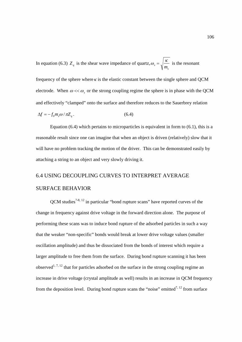
106

In equation (6.3) qZ is the shear wave impedance of quartz,s

s mkw = is the resonant

frequency of the sphere wherek is the elastic constant between the single sphere and QCM

electrode. When sww << or the strong coupling regime the sphere is in phase with the QCM

and effectively “clamped” onto the surface and therefore reduces to the Sauerbrey relation

qs Zmff pw /0-=D . (6.4)

Equation (6.4) which pertains to microparticles is equivalent in form to (6.1), this is a

reasonable result since one can imagine that when an object is driven (relatively) slow that it

will have no problem tracking the motion of the driver. This can be demonstrated easily by

attaching a string to an object and very slowly driving it.

6.4 USING DECOUPLING CURVES TO INTERPRET AVERAGE

SURFACE BEHAVIOR

QCM studies7-8, 12 in particular “bond rupture scans” have reported curves of the

change in frequency against drive voltage in the forward direction alone. The purpose of

performing these scans was to induce bond rupture of the adsorbed particles in such a way

that the weaker “non-specific” bonds would break at lower drive voltage values (smaller

oscillation amplitude) and thus be dissociated from the bonds of interest which require a

larger amplitude to free them from the surface. During bond rupture scanning it has been

observed1, 7, 12 that for particles adsorbed on the surface in the strong coupling regime an

increase in drive voltage (crystal amplitude as well) results in an increase in QCM frequency

from the deposition level. During bond rupture scans the “noise” emitted7, 12 from surface

107

particles as there bonds are broken is measured and plotted under the frequency vs. drive

voltage curve. These experiments show that a relative increase in frequency corresponds to a

spike in the noise spectrum analysis indicating bond breakage during that frequency shift.

The drive levels during bond rupture scans are relatively high and usually result in the

majority of the surface particles rolling, sliding, or hopping off the surface. A relative

increase in frequency does not strictly imply that the surface particles are leaving the surface.

It has been observed8 for particles in the strong coupling regime that relative changes in

frequency during rupture scans did result in the removal of particles from the surface. This

result suggest that the QCM is sensitive to the changes in the average coupling of particles

adhered to the surface as suggested by the SLA and Dybwad model discussed earlier. In our

experiments we ramp the drive voltage in a linear fashion first up to some maximum value

and back down to the starting position and record the frequency response. We call this

measurement a decoupling curve because it provides a qualitative interpretation of the

average bond strength of the particles adsorbed on the surface as they decouple from changes

in oscillation amplitude.

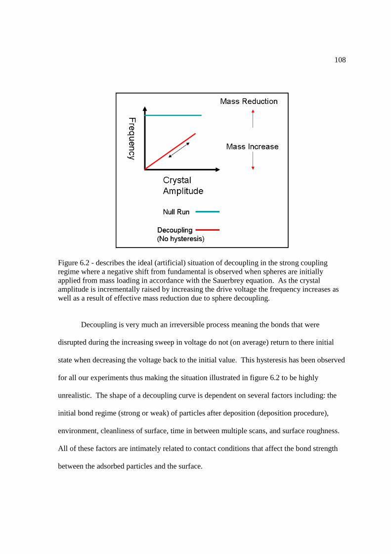
108

Figure 6.2 - describes the ideal (artificial) situation of decoupling in the strong coupling regime where a negative shift from fundamental is observed when spheres are initially applied from mass loading in accordance with the Sauerbrey equation. As the crystal amplitude is incrementally raised by increasing the drive voltage the frequency increases as well as a result of effective mass reduction due to sphere decoupling.

Decoupling is very much an irreversible process meaning the bonds that were

disrupted during the increasing sweep in voltage do not (on average) return to there initial

state when decreasing the voltage back to the initial value. This hysteresis has been observed

for all our experiments thus making the situation illustrated in figure 6.2 to be highly

unrealistic. The shape of a decoupling curve is dependent on several factors including: the

initial bond regime (strong or weak) of particles after deposition (deposition procedure),

environment, cleanliness of surface, time in between multiple scans, and surface roughness.

All of these factors are intimately related to contact conditions that affect the bond strength

between the adsorbed particles and the surface.

109

6.5 RESULTS AND DISCUSSION

Under the Derjaguin approximation13 for a sphere-on-sphere contacting geometry

(6.5)

epolystyrenadh RF gp2= (6.5)

in dry conditions where adhF is the adhesive force between the spheres, R is the radius of a

sphere, and epolystyreng is the surface energy of polystyrene we found that the force between

two 5 micron diameter and two 15 micron diameter spheres was Nm5.0 and

Nm5.1 respectively. Since the majority of our samples were deposited in air from aqueous

solution on samples on samples used directly from the package we assumed the force of

adhesion between the spheres electrode surface to be a combination of capillary adhesion

from water coupled with extra surface energy from contamination (hydrocarbons).

Assuming the meniscus force is the dominating factor for particle adhesion and arises mainly

from the capillary pressure we approximate the force of adhesion as

totalwet

adh RF gp4» (6.6)

where R is the radius of microsphere and

nhydrocarbowatertotal ggfg 2= . (6.7)

Equation (6.7) is the Good-Girifalco method14 which estimates the surface energy at

the contact. We are assuming that under these humid conditions as stated previously arises

from capillaries forming at the buried contacts between the sphere and electrode. Taking into

account the fact that the crystals were used as is we included the surface energy associated

110

with contamination ( nhydrocarbog ). The f term or “correction factor” was set to 0.5 to take into

account the mismatch in intermolecular interactions of water and hydrocarbons. We found

for m

mNwater 73=g and

mmN

nhydrocarbo 23»g that the force of adhesion wetadhF was equal to

approximately Nm2 and Nm6 for the 5 micron and 15 micron diameter spheres respectively.

These estimated forces are approximately 3 times the force which was calculated for

the interaction between microspheres. This implies that any spheres lying on top of spheres

that were directly adsorbed on the surface of the electrode (second order spheres) would in

principle move easier than the spheres attached to the surface (first order spheres). This

behavior was observed during an experiment performed in humid air (34% r.h.) for a sample

of mm5 diameter spheres deposited from aqueous solution on an 8 MHz QCM. This sample

was allowed to air dry over night before experiments were performed. We then performed 2

decoupling curve runs in the horizontal orientation where we observed no motion in the

optical region. Following immediately after the second horizontal decoupling curve run we

moved the sample to the vertical orientation and performed an additional decoupling curve

run where we again observed no motion in the optical region. We knew from previous

experiments that the spheres responded to abrupt changes in crystal amplitude. As a result

of this we performed our next experiment by rapidly and randomly varying the drive voltage

to induce particle motion. Before performing an experiment rapidly varying the QCM

amplitude we performed an additional decoupling curve figure 3a in the horizontal

orientation to gain some qualitative insight as to the varied average coupling strength in

response to changes in oscillation amplitude. We observed a negative shift in frequency

111

from natural resonance of 591 Hz which suggested that the particles were in the strong

coupling regime and equation (6.4) could be used to interpret there behavior. Applying

equation (6.4) we found approximately 17,550 where adsorbed on the surface. During the

forward sweep of our decoupling curve run we observed a slope change in the decoupling

curve around 110 mV indicating an increase in the average rate of particles decoupling. The

observed hysteresis during the backward sweep indicates that the particles restored to a

restored to a state of lower average coupling since the frequency at the return point has

increased from its initial value. After this decoupling curve (as mentioned earlier) we wished

to observe the particles dynamics since we were unable to do so during the decoupling scans.

The sample was mounted horizontally under normal lab air environmental conditions.

Images were taken in 2s intervals over a 10 minute period as we rapidly and randomly varied

the drive voltage in the range of the voltages used during the decoupling curve runs. Results

of this experiment are displayed in figures 6.4a and 6.4b where we observed a group of

second order spheres moving onto the surface of the electrode during the experiment while

no motion was observed during the entire experiment for first order spheres. This suggest

that the force of adhesion between spheres is less than force of adhesion between the spheres

and electrode as predicted earlier using equations (6.5), (6.6), and (6.7).

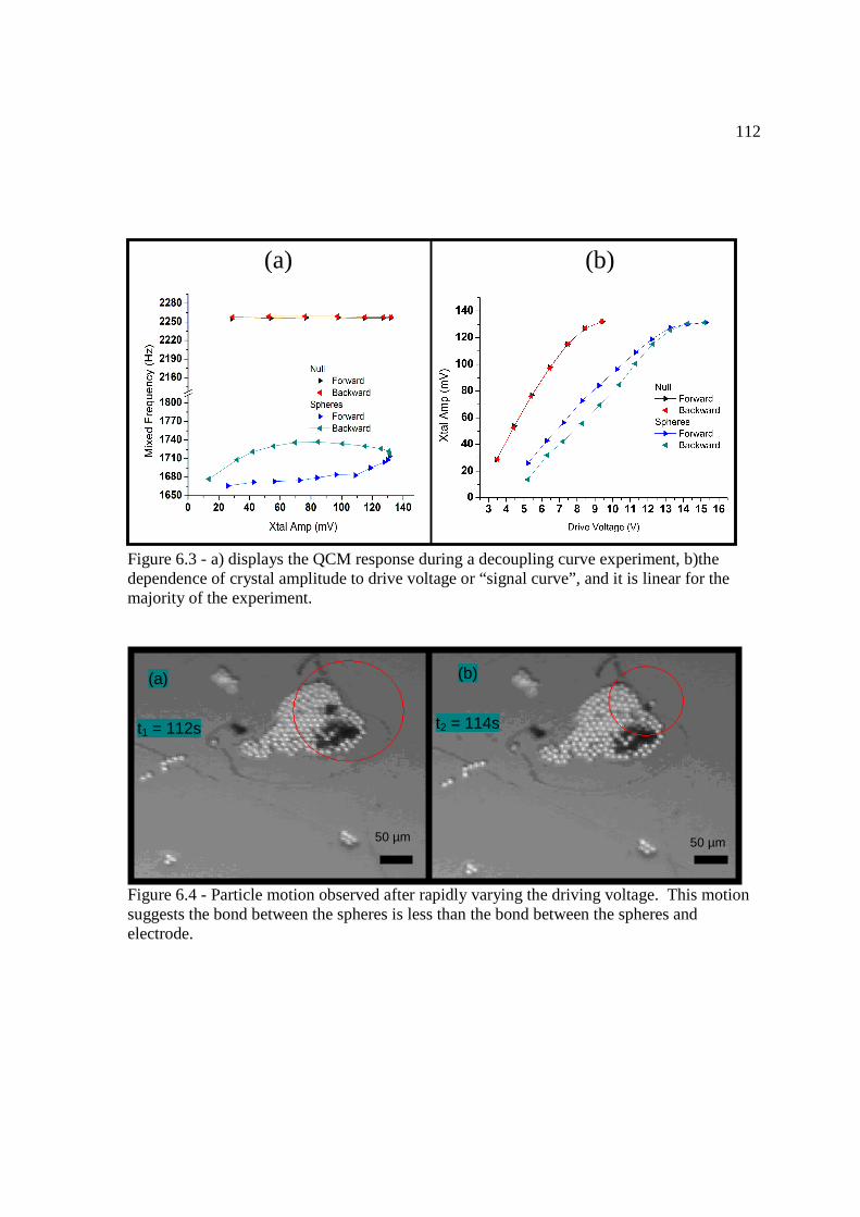
112

Figure 6.3 - a) displays the QCM response during a decoupling curve experiment, b)the dependence of crystal amplitude to drive voltage or “signal curve”, and it is linear for the majority of the experiment.

Figure 6.4 - Particle motion observed after rapidly varying the driving voltage. This motion suggests the bond between the spheres is less than the bond between the spheres and electrode.

50 µm 50 µm

(a) (b)

t1 = 112s t2 = 114s

(a) (b)

113

6.5.1 DYNAMICS UNDER FLOODED CONDITIONS

Figure 6.5 - Image of a QCM in 1 atm Nitrogen while rapidly varying the drive amplitude at large values to induce particle motion. This QCM had a substantial amount of water adsorbed onto the surface as a result of the deposition procedure (no drying time). As a result of the extreme shear forces produced by the QCM the adsorbed layer of water displayed an extreme amount of mobility.

Figure 6.2 describes the ideal situation of decoupling where a negative shift from

fundamental is observed when spheres are initially applied from mass loading in accordance

with the Sauerbrey equation. As the crystal amplitude is incrementally raised by increasing

the drive voltage the frequency increases as well as a result of effective mass reduction due to

sphere decoupling. Since sphere decoupling is energy dependent it is safe to suppose that

under ideal conditions such as a relatively flat and dry surface, that the decoupling curve

could in principle track itself during successive forward and backward runs within a drive

range below that which would induce particle motion. It is our experience that this has not

been the case. It was previously mentioned that the deposition conditions can have a

profound affect on the shape of decoupling curve. This was indeed the case for the

100 µm

114

decoupling curve shown in figure 6.6. This decoupling curve was performed in the

horizontal orientation in laboratory air. For this particular sample we did not allow it to dry

over night like the previously mentioned samples, meaning soon after the 5 micron diameter

spheres were deposited from aqueous solution decoupling curves were performed. We

observed an initial decrease in frequency after the spheres had been applied and for the most

part saw a linear increase in frequency with increasing crystal amplitude. Then when tracing

back to the original crystal amplitude we observed an interesting contradiction to the

decoupling model above and measured an increase instead of a decrease in QCM frequency

with decreasing amplitude. Upon repeating this run twice more we observed that the

hysteresis was removed however, the trend of the decoupling curve was opposite of the

model. These results imply that the surface behavior is more complex, and sphere

decoupling is not the only mechanism at work. For this particular sample sphere movement

was observed in the optical region at the higher amplitude values during the forward sweep.

This observation was true for the successive decoupling curve runs however, the observed

sphere motion decreased with additional runs.

This behavior is characteristic of the dynamics granular materials undergo experience

when there contacts are flooded. When the buried region between two contacting materials

(under capillary adhesion) becomes flooded the capillaries are broken thus weakening and

increasing the mobility between the two objects. This explanation is supported by the fact

we observed motion during decoupling curve runs for this experiment at lower crystal

amplitude values then what was observed for the previously mentioned experiment where the

sample was allowed to air dry over night. For the previously mentioned sample no motion

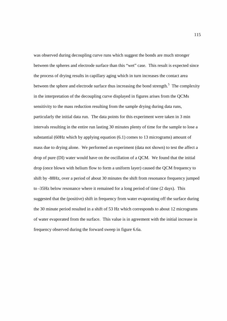
115

was observed during decoupling curve runs which suggest the bonds are much stronger

between the spheres and electrode surface than this “wet” case. This result is expected since

the process of drying results in capillary aging which in turn increases the contact area

between the sphere and electrode surface thus increasing the bond strength.5 The complexity

in the interpretation of the decoupling curve displayed in figures arises from the QCMs

sensitivity to the mass reduction resulting from the sample drying during data runs,

particularly the initial data run. The data points for this experiment were taken in 3 min

intervals resulting in the entire run lasting 30 minutes plenty of time for the sample to lose a

substantial (60Hz which by applying equation (6.1) comes to 13 micrograms) amount of

mass due to drying alone. We performed an experiment (data not shown) to test the affect a

drop of pure (DI) water would have on the oscillation of a QCM. We found that the initial

drop (once blown with helium flow to form a uniform layer) caused the QCM frequency to

shift by -88Hz, over a period of about 30 minutes the shift from resonance frequency jumped

to -35Hz below resonance where it remained for a long period of time (2 days). This

suggested that the (positive) shift in frequency from water evaporating off the surface during

the 30 minute period resulted in a shift of 53 Hz which corresponds to about 12 micrograms

of water evaporated from the surface. This value is in agreement with the initial increase in

frequency observed during the forward sweep in figure 6.6a.

116

5 10 15 20 25 30 35 40 458004100800412080041408004160800418080042008004220

8004310

8004320

8004330

8004340

8004350

Fre

quen

cy (

Hz)

Xtal Amp (mV)

null_forward null_backward 1st Sphere Run_forward 1st Sphere Run_backward 2nd Sphere Run_forward 2nd Sphere Run_backward

6 8 10 12 14 16 18 20 22

5

10

15

20

25

30

35

40

45

Xta

l Am

p (m

V)

Drive Voltage (V)

null_forward null_backward 1st Sphere Run_forward 1st Sphere Run_backward 2nd Sphere Run_forward 2nd Sphere Run_backward

(a) (b)

Figure 6.6 - (a) shows the behavior of the initial decoupling curve performed on this QCM as well a second decoupling curve followed soon after. The signal curves (b) are displayed for each data run and show that the oscillation amplitude depended linearly on the drive voltage from our power supply.

Motion was observed within the first ten minutes of the decoupling curve as shown in

the figures 6.7a and 6.7b. No additional motion was observed until the maximum drive

voltage was reached in which the motion on the surface was substantial. For the most part

microspheres moved in the direction of oscillation however, as shown in the figures this was

not the case for all of the mobile spheres on the surface.

117

Figures 6.7 - a) and b) are images taken during the initial horizontal orientation decoupling curve run, these images were taken 3 minutes apart from each other and correspond in time to the boxed region of the decoupling curve. The increased energy from the rise in oscillation amplitude from figure 6.7a to 6.7b, aided in breaking the necessary bonds to translate the circled sphere from the cluster in which it belonged. The circled sphere is a “first order” or bottom layer sphere that moves roughly in the oscillation direction.

6.5.2 ENVIRONMENTAL INFLUENCE ON FRICTION

In a study4 performed by Flanigan et. al. the researches demonstrated how a QCM

could be used to probe contact mechanics. They found that the (negative) shift in resonate

frequency of a QCM in response to a viscoelastic loading material (such as the spheres we

used in our experiments they used gel caps) is linearly dependent with the (real) contact area

Initial decoupling photos in horizontal orientation

Images were taken in 3 minute intervals. The total time for this decoupling curve was approximately thirty minutes.

50 microns

50 microns

Oscillation Direction

Oscillation Direction

5 10 15 20 25 30 35 40 458004110

8004120

8004130

8004140

8004150

8004160

8004170

8004180

8004190

8004200

8004210

8004220

Fre

quen

cy(H

z)

Crystal Amplitude(mV)

Forward Backward

Figure 7a

Figure 7b

The majority of the observed motion occurred in this region.

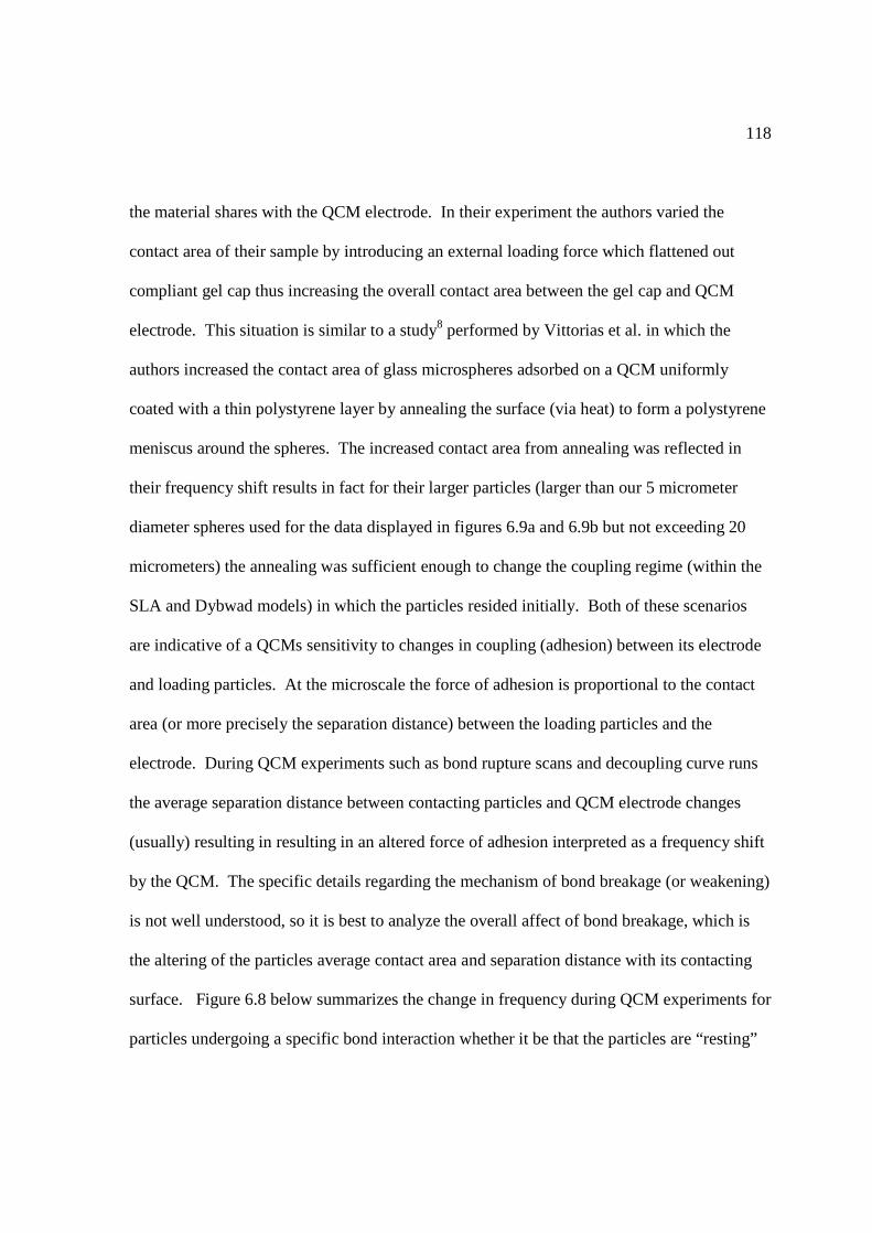
118

the material shares with the QCM electrode. In their experiment the authors varied the

contact area of their sample by introducing an external loading force which flattened out

compliant gel cap thus increasing the overall contact area between the gel cap and QCM

electrode. This situation is similar to a study8 performed by Vittorias et al. in which the

authors increased the contact area of glass microspheres adsorbed on a QCM uniformly

coated with a thin polystyrene layer by annealing the surface (via heat) to form a polystyrene

meniscus around the spheres. The increased contact area from annealing was reflected in

their frequency shift results in fact for their larger particles (larger than our 5 micrometer

diameter spheres used for the data displayed in figures 6.9a and 6.9b but not exceeding 20

micrometers) the annealing was sufficient enough to change the coupling regime (within the

SLA and Dybwad models) in which the particles resided initially. Both of these scenarios

are indicative of a QCMs sensitivity to changes in coupling (adhesion) between its electrode

and loading particles. At the microscale the force of adhesion is proportional to the contact

area (or more precisely the separation distance) between the loading particles and the

electrode. During QCM experiments such as bond rupture scans and decoupling curve runs

the average separation distance between contacting particles and QCM electrode changes

(usually) resulting in resulting in an altered force of adhesion interpreted as a frequency shift

by the QCM. The specific details regarding the mechanism of bond breakage (or weakening)

is not well understood, so it is best to analyze the overall affect of bond breakage, which is

the altering of the particles average contact area and separation distance with its contacting

surface. Figure 6.8 below summarizes the change in frequency during QCM experiments for

particles undergoing a specific bond interaction whether it be that the particles are “resting”

119

in place experiencing constant contact (separation distance remains constant on average)

throughout the entire experiment (6.8a and 6.8b) or that there contact area and perhaps the

separation distance is changing throughout the experiment as a result of friction (6.8c and

6.8d). We assume that the force of adhesion at the scale of our experiments is dominated by

two main forces Van der Waals and capillary respectively. These forces are both dependent

on the separation distance at the contact and are15

26D

RAF Hvdw

adh = (6.8)

DAF l

mencap

adh

g2= (6.9)

where HA ,R,D are the Hamaker constant, radius of particle, and separation distance

respectively for equation (6.8). The terms menA , lg , and D are the area of the flooded contact

region, surface energy/tension of the liquid layer (in our case water), and the separation

distance respectively. When analyzing the observed behavior for the wet environment

associated for our experiments we expect that equation (6.9) provides the most relevant

interpretation.

120

Figure 6.8 - describes the predicted response of the change in QCM frequency to oscillation amplitude when the adsorbed particles are undergoing a particular frictional interaction between its contact with the surface. These scenarios have shown up in the literature before8 with the added component of the

change in bandwidth (dissipation) with oscillation amplitude.

Δf Δf

Δf Δf

Hookean Spring

Viscoelastic Contact

Mindlin Partial Slip

Coulomb Friction

Xtal Amp

Xtal Amp

Xtal Amp

Xtal Amp

(d) (c)

(b) (a)

121

5 10 15 20 25 30 35 40

-225

-210

-195

-180

-165

5 10 15 20 25 30 35 40

-156

-153

-150

-147

-144

Df (

Hz)

Xtal Amp (mV)

1st Sphere Run_foward

Df (

Hz)

Xtal Amp (mV)

2nd Sphere Run_foward

20 40 60 80 100 120 140-600

-590

-580

-570

-560

-550

-540

Df (

Hz)

Xtal Amp (mV)

Sphere Run_forward

(a) (b)

Figure 6.9 - (a) is the change in frequency with respect to crystal amplitude for the decoupling curve experiment shown in figure 3a. The to plots in (b) are the change in frequency with respect to crystal amplitude for the “wet” decoupling curve experiments displayed in figure 6a for the forward runs during the first and second sweeps.

According to figure 6.8 the trends displayed in both 6.9a and 6.9b are indicative of

Coulomb type friction. This is quite possible for the experiment illustrated by plot 6.9a

where the particles were clamped to the surface by capillary aging. This observation is

similar to the situation described in the Vittorias et. al. study8 for the case of annealed

particles where they too observed Coulomb like friction behavior for clamped particles. For

our experiments the environmental conditions along with the varying oscillation amplitude

during decoupling curve runs influenced the contact area between our particles and the

electrode. Even though the initial or “first sphere run” displayed in figure 6.9b suggest a

Coulomb friction mechanism we realized that the majority of the observed behavior was a

result of water drying on the surface due to the wet surface conditions which has little to do

with the actual sphere decoupling friction mechanism. We therefore began our analysis of

the observed sphere behavior at the “second sphere run” which according to 6.8c suggest a

122

“Mindlin16 microslip” friction mechanism. However, after applying friction analysis

mentioned in chapters 3 and 5 the frictrion law was primarily viscous (n=1.05). We illustrate

in figure 10 an alternate mechanism that could result in the trend observed in figures 6.8c and

6.9b (run 2) for spheres in wet conditions (flooded contacts).

Figure 6.10 - Illustrates a mechanism that explains the trend displayed in figures 6.8c and 6.9b run 2 with out the presence of microslip. At increasing amplitude water in the flooded contact experiences an increase in mobility that draws the microsphere closer to the substrate increasing the loading force resulting in a negative shift in frequency.

The scenario shown in figure 10 is supported by the observed (figure 6.5) mobility of

water on the surface of an oscillating QCM. Under these wet conditions it is reasonable to

assume that the majority of the adsorbed spheres on the surface have there entire “buried”

contact area flooded with water from the surface. At the lowest drive levels the water buried

with in the contact has the lowest level of mobility and mainly serves to reduce the adhesive

force with the surface (compared to when it is clamped down in solid-solid contact like the

experiment shown in figure 6.9a) by increasing the separation distance between the sphere

123

and the QCM electrode which supports why we observed particle motion early in our

decoupling curve (figure 6.7). As the oscillation amplitude is increased the buried water

layer becomes more mobile as a result of the increase in shear force and therefore gains a

sufficient amount of energy to escape the buried contact region which draws the particle

closer to the surface as a result of the shear force exceeding the meniscus force as illustrated

in Figure 6.10 above. One main implication of this mechanism is that the oscillation

amplitude is sufficient to remove the water from the buried contact and induce mobility, we

expect that as time increases and the contacts are able to dry this process becomes

exceedingly difficult and will require larger drive levels to release the buried water. For

some critical drying time this “wet decoupling process” will move shift to the strong

coupling regime of the SLA and Dybwad models which was exactly what we observed for

figures 6.3A and 6.9A.

6.5.3 DYNAMICS IN “DRY” CONDITIONS (TRANSFER EXPERIMENT)

In an effort to reduce the affect that capillaries have during QCM experiments and to

analyze particle dynamics in a drier and thus more controlled environment we performed

particle transfer experiments. In these experiments we deposited 15 micron diameter

microspheres from aqueous solution in the usual manner on the electrode of a 5 MHz “gun”

crystal. Our experimental 8 MHz “target” crystal was oriented below the gun to

catch particles during the procedure. The transfer experiments were performed in a dry

(approximately 1 atm of nitrogen gas) environment. After performing the experiment we

observed particle motion during decoupling curve sweeps even though the majority of the

particles landed in regions away from the center of the electrode where the oscillation

124

amplitude is highest. No such motion was observed for similar crystal amplitudes during

experiments where the particles were left to air dry after deposition even though they were

deposited at the center of the electrode. This observation supports that the transferred

spheres from the “gun” QCM are landing on the target QCM and forming a weaker bond

with the surface which is what is expected for a drier contact.

Figure 6.11 - Image taken after completing a successful transfer experiment.

Gun QCM (5 MHz)

Target QCM (8 MHz)

150 µm

125

Figure 6.12 - Decoupling curves of the target QCM before and after the transfer experiment was performed.

The null run in figure 6.12 suggest that the target QCM was not clean and it was

likely that a thin film of water along with containments were present on the sample. The

trend suggest that the contamination particles were undergoing a wet decoupling friction

mechanism. After successful transfer we observed a negative shift from resonance of 12 Hz

which after applying equation (6.4) amounts to approximately 13 spheres on the electrode

surface. After analyzing the surface via optical microscopy (figure 6.14) we counted a total

of approximately 82 spheres which amounted to a considerable difference. This difference

was of no surprise to us as a result of several factors. The first and possibly the most

important factor is the fact that only a very small fraction of the spheres landed near the

center of the QCM electrode where the sensitivity is a maximum9 and falls off in a Gaussian

manner radially outward. Another factor that influenced this difference was the fact that

0.01 0.02 0.03 0.04 0.05 0.06 0.07 0.08 0.09

8009988

8009992

8009996

8010000

8010004

8010008

8010012

8010016

Fre

quen

cy (

Hz)

Voltage (V)

Run 1_forward Run 1_backward null before transfer_forward null before transfer_backward

No spheres on surface

Spheres on surface

126

particles of this size have been observed in the literature8 to fall with in the intermediate

range between strong and weak coupling where analysis is much more difficult. This

transition was indeed observed in Figure 6.13 which shows an abrupt change in friction

mechanism as a result of this newly formed contact from transfer. We compare these curves

to a 15 micron decoupling curve experiment (Figure 6.14) performed under usual

atmospheric conditions (lab air) and deposited from aqueous solution, the sample was then

allowed a day to air dry.

-2.70 -2.65 -2.60 -2.55 -2.50-20.5

-20.0

-19.5

-19.0

-18.5

-18.0

region 3

Run 1_region 3 Linear Fit of ln(slip time)

ln(s

lip ti

me)

(s)

ln(Xtal Amplitude) (V)

slope = 9.5

n = 0.09

Coulomb like

0.02 0.03 0.04 0.05 0.06 0.07 0.08 0.09

-24

-22

-20

-18

-16

-14

-12

-10 Run 1 after transfer_forward

DF

Xtal Amplitude (V)

region 1

region 2

region 3

-3.8 -3.7 -3.6 -3.5 -3.4 -3.3 -3.2 -3.1-18.10

-18.05

-18.00

-17.95

-17.90

-17.85

-17.80 region 1


ln(s

lip ti

me)

(s)


slope = - 0.3

n = 1.4

Mindlin like

-3.1 -3.0 -2.9 -2.8 -2.7-20.5

-20.0

-19.5

-19.0

-18.5

-18.0 region 2


ln(s

lip ti

me)

(s)


slope = -4.67

n = - 0.27

Figure 6.13 – Friction analysis of the target QCM after the transfer experiment was performed.

(a)

(c)

(b)

(d)

127

We observed particle motion (as indicated in figures 6.13a and 6.13b) spheres caught

during the transfer experiment. This motion was first observed right around the time the

friction mechanism changed as indicated by the varied trend in 6.13b. At the critical

amplitude of 65 mV the particles experienced a Coulomb like friction law. This could be

explained by the fact that the water layer the spheres are sliding on is very thin (perhaps even

solid-like17) and as a result experiences a larger viscous force than would be expected

normally (like in experiments displayed in 6.7a and 6.7b). If we think of it this way then

when the oscillation amplitude is sufficient for supplying a shear force that overcomes the

films viscosity (or yield stress if solid like) then the bond breaks and the interaction is the

same as what was observed for particles in the strong coupling regime figure 6.3a.

0.015 0.020 0.025 0.030 0.035 0.040 0.045 0.0507999888

7999890

7999892

7999894

7999896

7999898

7999900

7999902

7999904

7999906

7999908

run 2_forward run 2_backward

Fre

quen

cy (

Hz)

Xtal Amplitude (V)

0.020 0.025 0.030 0.035 0.040 0.045 0.050-190

-185

-180

-175

-170

-165

n = -2.6

n = 0.6mixed law

Df (

Hz)

Xtal Amplitude (V)

n = -3.3

Figure 6.14 - Friction analysis of 15 micron microsphere sample deposited from aqueous solution. The sample was in the strong coupling regime of the Dybwad (SLA) model. The decoupling curve shown in figure 6.14a exhibits a “stick-slip” like behavior as the

amplitude increases to about 35 mV (the “mixed law” region). Figure 6.14b shows that the

friction law transitions but does not change it’s inverse dependence on velocity. This lack of

(a) (b)

128

alteration in friction mechanisms was the main difference between the dry and “semi-wet”

(figure 6.14ab) experiments. Another difference is the appearance of Mindlin like partial slip

in the dry experiment which is not present in the wet experiment.

Figure 6.15 - The image above is a reconstruction of the QCMs used after the transfer experiment was performed. Each tile is an image with the dimensions of our optical region when adjusting the resolution to illuminate the spheres on the surface. Scratches were intentionally placed on the surface to provide a reference point when analyzing the distance from one image to another when spheres move on the surface. The highlight region is of a sphere caught near the edge of quartz where the QCM sensitivity would be minimal.

Shadow of 5MHz“gun” QCM

30 µm

129

Figure 6.16 - The above photo consist of two images superimposed onto each other. The first image is of the surface oriented in the horizontal orientation and the second image is after the sample has been rotated in the vertical orientation where gravity has an affect. We observed particle motion on the rough (quartz) crystal side circled to the right due to gravity alone whereas no motion was observed for the particles that landed on the smoother polished gold electrode.

It was expected that the presence of microscale roughness greatly reduces the force of

adhesion between two solids in contact. Figure 6.16 supports that the particles are indeed

“drier” as indicated by the observed movement of a cluster of spheres on the rougher quartz

region of the crystal from gravity alone. This observation supports the idea that roughness

increases the separation distance between the particle and substrate which in turn weakens

the force of adhesion (Van der Waals) which is inversely proportional to the square of the

separation distance. If the particles on the quartz were wet at the contact the increased

roughness of the quartz would have less of an effect on the force of adhesion which would be

primarily a result of the liquid meniscus force. Since the landed particles are presumably

drier there attraction to the surface would result from a Van der Waals interaction which is

Gravity

130

sufficient to hold them on the surface (provided the separation distance between the particles

and the surface is small enough).

6.5.4 DYNAMICS IN VARIED ENVIRONMENTAL CONDITIONS

Several decoupling curve experiments were performed in the vacuum chamber to

observe how altering the environment of a sample affects the friction. These experiments

were performed on a sample with 5 micron diameter spheres deposited from aqueous

solution. No motion was observed in the optical region during these decoupling curve runs.

Friction laws (n) for these experiments were determined using methods outlined in chapters 3

and 5 of this thesis. All of the experiments resided in the strong coupling regime of the

Dybwad model which allowed for calculation of slip times. These slip time values were

computed relative to the inertial loading point (largest (magnitude) shift in frequency from

resonance) as shown in figure 6.17. The runs performed in air and vacuum show similar

decoupling curve trends as well as friction laws. The vacuum experiment resulted in a

slightly more viscous like friction law (less decoupling) which suggested that the average

particle adhesion increased as a result of introducing vacuum. The dry nitrogen environment

showed transition if frictional behavior from a “slightly more viscous” than “Coulomb like”

friction law to a slipping mechanism that was inversely proportional to the cube of velocity.

This type of friction law ( nvF -µ ) was observed in the decoupling curve experiments

performed on 15 micron spheres (figures 16.14ab). The implication from this result is that

the removal excess water layers on the surface can cause 5 micron spheres that strongly

bonded to the surface and behave like ordinary physisorbed systems into a slipping

mechanism similar to what was observed for the larger 15 micron particles.

131

5 10 15 20 25 30 35 40 45 50 55 60 65 707990700

7990710

7990720

7990730

7990740

7991300

7991310

7991320

7991330

7991340

7991350

Last run in N2 778 torr_H^2 Run 1 in N2 778 torr_H^2 Run 2 in vac_H^2 Run 1 in vac_H^2 Run 5 in air_H^2 Run 1 in air_H^2 Null Run_H^2 Null Run_H^2

Fre

quen

cy (

Hz)

Xtal Amplitude (mV)

no spheres

with spheres

inertial loading point

Figure 6.17 - Decoupling curves (forward runs only) for the same sample studied in the varied environments of air, vacuum (1E-3 torr), and dry nitrogen (N2). The H^2 denotes that the mounting orientation is horizontal or parallel with the surface (normal to gravity).

2.0 2.2 2.4 2.6 2.8 3.0 3.2 3.4 3.6 3.8

-19.9

-19.8

-19.7

-19.6

-19.5

-19.4

-19.3

-19.2

-19.1

-19.0 Run 1 in air

H^2 run 1 in air Linear Fit of ln(slip time)

ln(s

lip ti

me)

(s)

ln(xtal amp) (mV)

n=0.67

slope = 0.5

5 10 15 20 25 30 35 407990705

7990710

7990715

7990720

7990725

7990730

7990735

7990740

7990745

7990750

Fre

quen

cy (

Hz)

Xtal Amplitude (mV)

Run 1 in air_H^2 Run 1 in air_H^2

Run 1 in air

Figure 6.18 -First decoupling curve run in air (approximately 35% r.h.) is shown in (a). The friction analysis of the forward sweep in the decoupling curve is shown in (b).

132

2.0 2.2 2.4 2.6 2.8 3.0 3.2 3.4 3.6 3.8

-20.1

-20.0

-19.9

-19.8

-19.7

-19.6

-19.5

-19.4

-19.3

H^2 run 1 in vac Linear Fit of ln(slip time)

ln(s

lip ti

me)

(s)

ln(xtal amp) (mV)

n=0.73

slope = 0.37

Run 1 in vacuum 1E-3 torr

5 10 15 20 25 30 35 40 457990700

7990705

7990710

7990715

7990720

7990725

7990730

7990735

7990740

Run 1 in vac 1E-3 torr

Fre

quen

cy (

Hz)

Xtal Amplitude (mV)

Run 1 in vac_H^2 Run 1 in vac_H^2

Figure 6.19 - First decoupling curve run in 1E-3 torr vacuum environment is shown in (a). The friction analysis of the forward sweep in the decoupling curve is shown in (b).

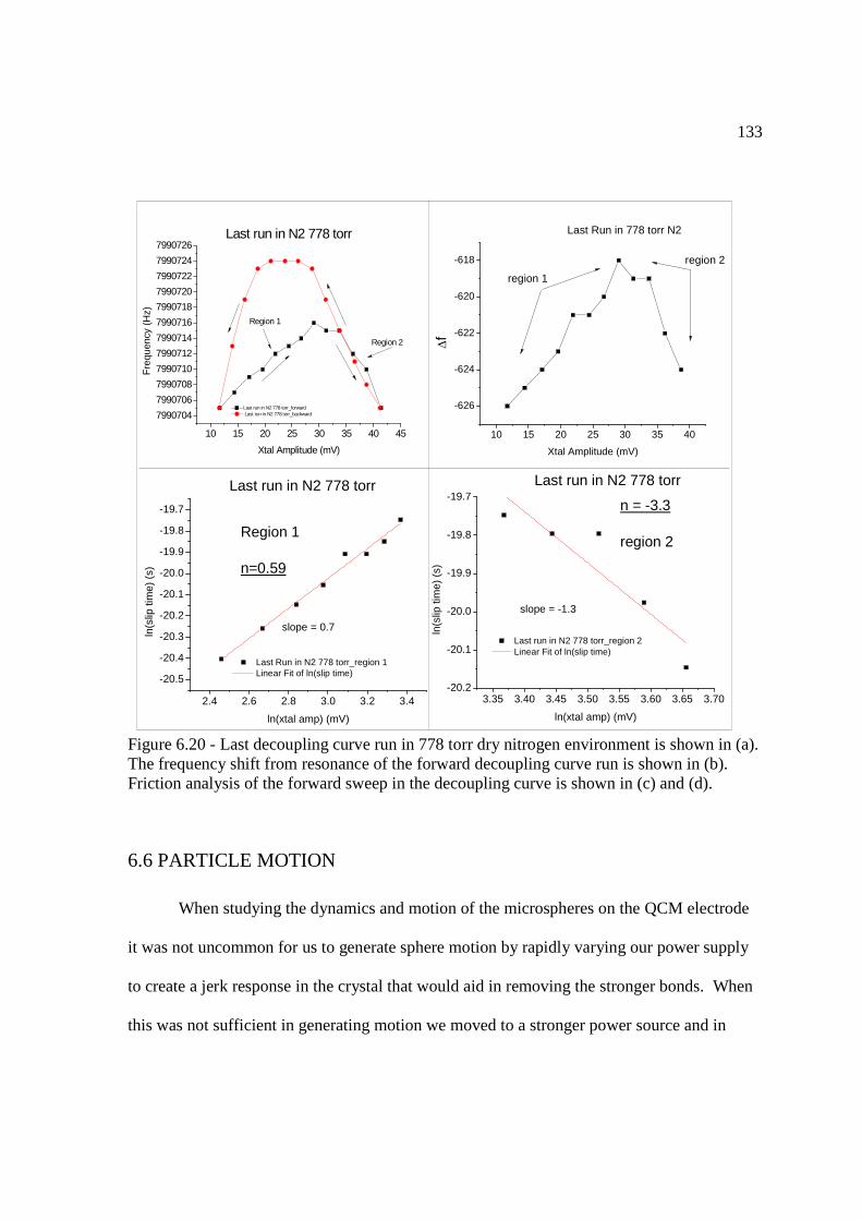
133

10 15 20 25 30 35 40 45

7990704

7990706

7990708

7990710

7990712

7990714

7990716

7990718

7990720

7990722

7990724

7990726Last run in N2 778 torr

Last run in N2 778 torr_forward Last run in N2 778 torr_backward

Fre

quen

cy (

Hz)

Xtal Amplitude (mV)

Region 1

Region 2

2.4 2.6 2.8 3.0 3.2 3.4

-20.5

-20.4

-20.3

-20.2

-20.1

-20.0

-19.9

-19.8

-19.7

Last run in N2 778 torr

Last Run in N2 778 torr_region 1 Linear Fit of ln(slip time)

ln(s

lip ti

me)

(s)

ln(xtal amp) (mV)

Region 1

n=0.59

slope = 0.7

3.35 3.40 3.45 3.50 3.55 3.60 3.65 3.70-20.2

-20.1

-20.0

-19.9

-19.8

-19.7Last run in N2 778 torr

Last run in N2 778 torr_region 2 Linear Fit of ln(slip time)

ln(s

lip ti

me)

(s)

ln(xtal amp) (mV)

slope = -1.3

n = -3.3

region 2

10 15 20 25 30 35 40

-626

-624

-622

-620

-618 region 2

Last Run in 778 torr N2

DfXtal Amplitude (mV)

region 1

Figure 6.20 - Last decoupling curve run in 778 torr dry nitrogen environment is shown in (a). The frequency shift from resonance of the forward decoupling curve run is shown in (b). Friction analysis of the forward sweep in the decoupling curve is shown in (c) and (d).

6.6 PARTICLE MOTION

When studying the dynamics and motion of the microspheres on the QCM electrode

it was not uncommon for us to generate sphere motion by rapidly varying our power supply

to create a jerk response in the crystal that would aid in removing the stronger bonds. When

this was not sufficient in generating motion we moved to a stronger power source and in

134

doing so observed some very interesting behavior. The microspheres on the surface of a

QCM experience an extreme shear force resulting from the high frequency oscillation of the

QCM that governs there observed surface dynamics. The rapidly changing direction of this

force causes particles to “ratchet” along the surface of the electrode. A maximum value for

the distance a microsphere (we report here results for the 5 micron diameter spheres) travels

for the duration the peak force acts on the sphere can be approximated provided a few

assumptions. The first assumption is that kinematic equations apply for the non inertial

reference frame of an oscillating QCM. If we solve the problem for the time ( )02/1 f at

which the peak force acts on the microsphere we find that this force acts in one direction

making it a reasonable approximation to assume the acceleration is constant thus allowing

the use of kinematic equations. The next assumption is that the microsphere is stationary

which is artificial since the microsphere before detachment is initially moving at a velocity

equal to the velocity of the QCM however, the direction in which that vector is pointing is

not so obvious due to a lack of knowledge regarding the bond rupture mechanism. As a

result we assume set the initial velocity to zero to provide an “order of magnitude”

approximation of sliding distance. In the absence of friction the one dimensional sliding

distance becomes2

2pA were A is the oscillation amplitude of the QCM. An oscillation

amplitude A=21nm (which was easily achieved by our strong power source) would result in a

sliding distance of 0.1 microns. The shortest time span we could observe with our dvd

recorder was 0.01s. The measurement of 0.1 microns was for the duration of half an

oscillation period, in the unlikely case that in 0.01s or 80,000 periods this force only induced

135

motion in one direction during the observation time a sphere would travel approximately 640

m or 0.4 miles. We stated previously that particles tightly bound to the surface via capillary

interaction are more likely to undergo a coulomb type friction mechanism during bond

rupture. Inserting this resistive term into our distance approximation we obtain

úû

ùêë

é-=

20

22

42 fm

FA

nd

s

adhkoddsliding

mp . (6.10)

where nodd is the total number of odd cycles (periods), A is the amplitude of oscillation, km is

the coefficient of kinetic friction, adhF is the force of adhesion (capillary or Van der Waals),

kgms14107 -´= is the mass of the loading (5 micron diameter) particle, and 0f is the

resonant frequency (8 MHz) of QCM.

Plugging in typical values 5.0=km and NFF capadh m2== results in a decrease of

approximately 55 nm per half cycle which would result in a sliding distance over a period

0.01s to now be 228 m or 0.1 miles which is an appreciable decrease in motion. This

example is of course highly unrealistic since the particle has an “equal” probability to be

translated in either direction along the surface. When analyzing the dynamics this competing

aspect is immediately obvious especially when drive levels are high and motion is

substantial. In the Vittorias8 experiment they observed 3 main modes scenarios of particle

dynamics from analyzing deformation patterns. They found that it is not uncommon for

microspheres to remain at one location for a large number of periods before sliding. The

authors observed shear deformation patterns which indicates the spheres were sliding

however, this does not rule out the possibility of rolling. One particularly interesting

observation was particles leaving the surface in via hopping from place to place. We hooked

136

the sample shown in figure 6.5 up to our strong power source to stimulate particle motion on

this wet surface. We observed many interesting dynamics including the hopping described

earlier. Particles generally moved in along the direction of oscillation however, if they were

confined in cracks or defects on the surface the followed the path of the defect or pinning site

until the oscillation was sufficient to eject it from its potential barrier. This may aid in

achieving controlled or at the very least enhancing microparticle manipulation and control

via intentional defect regions for “guiding” microparticles. We also observed what appeared

to be motion influenced by charge interactions between microparticles. These cases involved

microspheres in sync with out actually touching its neighbor. Since our surface was wet we

observed many interesting dynamics influenced by the water on the surface. For aggregated

microsphere islands whose contacts were completely immersed we observed in real time the

water ejecting from the many contacts within the island.

137

Conclusion Figure 6.21 - Dynamics of a partially immersed cluster of aggregated spheres during rapidly varying the drive voltage of our strong power source. We observed that the shear stresses were sufficient enough to squeeze water from confined regions within the cluster.

In this study we have demonstrated methods for interpreting average particle

behavior on during QCM experiments mainly through realizing the possibility of wet

decoupling. We have shown overwhelming evidence that the effects of water during QCM

experiments can not be ignored and in many cases govern the dynamics as a whole on the

surface. The affects of dissipation (bandwidth shift) were not reported on in this study

however, it is important to realize that water will have a huge affect on the dissipation data

especially under a wet decoupling mechanism. We introduced a new method for decreasing

the presence of water during QCM experiments and provided sufficient evidence that upon

landing the overall system force of adhesion is greatly reduced and reflected in both the

decoupling and delta frequency plots. Particle transfer experiments have the potential for

many fundamental applications of better understanding the friction mechanism at microscale.

It is possible with a customized chamber one could measure the friction force directly after a

transfer experiment by orienting the chamber vertically (figure 6.16) in a controlled manner

recording the dynamics and rotation angle during the experiment. In this study we have

138

found that the analysis of decoupling curves can be quite complex due to the inconsistent

bond strength of the spheres on the surface and the multiple paths spheres can take once in

motion. Due to the nature of the deposition and the sub-monolayer surface configuration

hysteresis and non uniformity can somewhat be expected in these decoupling curves. The

notion of micro particle sorting as suggested by the observed particle motion is not a straight

forward task especially in humid/wet environments. However, it may be easier to achieve

such control and sorting in a dry environment such as particles on the surface after a transfer

experiment. Future work must be done to see if movement can be better controlled and

understood.

Acknowledgments:

The authors would like to acknowledge Edward Stevens for his help in constructing images.

139

6.7 REFERENCES

1. Hirst, E. R.; Yuan, Y. J.; Xu, W. L.; Bronlund, J. E., Bond-rupture immunosensors--A review. Biosensors and Bioelectronics 2008, 23 (12), 1759-1768. 2. Rivet, C.; Lee, H.; Hirsch, A.; Hamilton, S.; Lu, H., Microfluidics for medical diagnostics and biosensors. Chemical Engineering Science 2011, 66 (7), 1490-1507. 3. Dybwad, G. L., A sensitive new method for the determination of adhesive bonding between a particle and a substrate. Journal of Applied Physics 1985, 58 (7), 2789-2789. 4. Flanigan, C. M.; Desai, M.; Shull, K. R., Contact Mechanics Studies with the Quartz Crystal Microbalance. Langmuir 2000, 16 (25), 9825-9829. 5. D'Amour, J. N.; Stålgren, J. J. R.; Kanazawa, K. K.; Frank, C. W.; Rodahl, M.; Johannsmann, D., Capillary Aging of the Contacts between Glass Spheres and a Quartz Resonator Surface. Physical Review Letters 2006, 96 (5), 058301-058301. 6. Ellis, J. S.; Thompson, M., Acoustic physics of surface-attached biochemical species. HFSP Journal 2008, 2 (4), 171-177. 7. Dultsev, F. N.; Ostanin, V. P.; Klenerman, D., “Hearing” Bond Breakage. Measurement of Bond Rupture Forces Using a Quartz Crystal Microbalance. Langmuir 2000, 16 (11), 5036-5040. 8. Vittorias, E.; Kappl, M.; Butt, H.-J.; Johannsmann, D., Studying mechanical microcontacts of fine particles with the quartz crystal microbalance. Powder Technology 2010, 203 (3), 489-502. 9. Seah, P. J. C. a. M. P., The quartz crystal microbalance; radial/polar dependence of mass sensitivity both on and off the electrodes. Measurement Science and Technology 1990, 1 (7), 544-555. 10. Sauerbrey, G., Verwendung von Schwingquarzen zur Wägung dünner Schichten und zur Mikrowägung. Zeitschrift für Physik 1959, 155 (2), 206-222. 11. Johannsmann, D., Viscoelastic, mechanical, and dielectric measurements on complex samples with the quartz crystal microbalance. Physical Chemistry Chemical Physics 2008, 10 (31), 4516-4516. 12. (a) Dultsev, F. N.; Speight, R. E.; Fiorini, M. T.; Blackburn, J. M.; Abell, C.; Ostanin, V. P.; Klenerman, D., Direct and Quantitative Detection of Bacteriophage by “Hearing” Surface Detachment Using a Quartz Crystal Microbalance. Analytical Chemistry 2001, 73

140

(16), 3935-3939; (b) Cooper, M. A., Biosensing using rupture event scanning (REVS) . Measurement Science and Technology 2003, 14 (11), 1888-1893. 13. Derjaguin, B., Untersuchungen über die Reibung und Adhäsion, IV - Theorie des Anhaftens kleiner

Teilchen. Kolloid-Zeitschrift 1934, 69 (2), 155-164. 14. Israelachvili, J., Intermolecular and Surface Forces. Elsevier: (1985-2004); Vol. 2. 15. Mate, C. M., Tribology on the small scale a bottom up approach to friction,lubrication, and wear. Oxford University Press: New York, 2008; Vol. 1, p 333. 16. Deresiewicz, R. D. M. a. H., Elastic spheres in contact under varying oblique forces. Journal of Applied Mechanics 1953, 20, 327-344. 17. Peachey, J.; Van Alsten, J.; Granick, S., Design of an apparatus to measure the shear response of ultrathin liquid films. Review of Scientific Instruments 1991, 62 (2), 463-463.

141

CHAPTER 7 – STUDIES OF DYNAMICS OF MICROSPHERES

IN VARIED FRICTION REGIMES

7.1 WATER DECOUPLING EXPERIMENT IN AIR

In the sections that follow below unless otherwise stated I deposited 15 micron polystyrene

sphere from aqueous solution onto the electrode of a QCM in ordinary (30% - 40% rh) lab

air. With this in mind a baseline experiment was performed to show the effect a dried water

layer has on the surface of our experimental QCM. This baseline was important in

determining the true “null” frequency behavior of our sample. When analyzing the frictional

behavior of the microspheres deposited on the surface it was extremely important to have the

proper mass loading frequency value so that slip time (frictional) measurements would be as

accurate as possible. The water droplet was deposited in the same manner as microspheres.

It was drawn from a glass pipette and blown with helium flow to remove bulk water layers,

the sample was then left out to air dry overnight before experiments were performed. The

results of this experiment are displayed below in figure 7.1. The dried water layer is in the

strong coupling regime of the Dybwad model1 (negative shift from resonance) which means

the particles are strongly coupled to the surface and the Sauerbrey equation2 can be used to

approximate the mass of the film which is approximately 70 ng. Friction laws “n” and slip

times were calculated using methods outlined in chapters 3, 5, and 6 of this thesis. As shown

in figure 7.1 (b) the frictional behavior throughout a forward sweep of a decoupling curve is

not always uniform and thus the plots are split into regions in order to obtain a more detailed

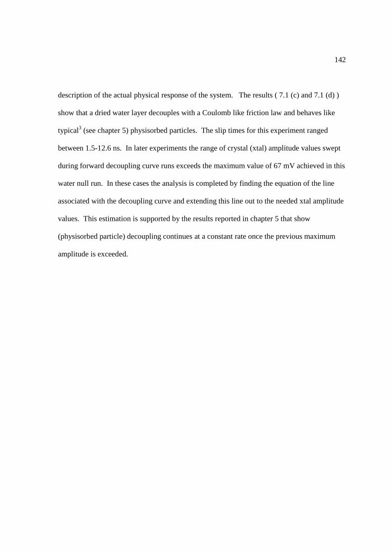
142

description of the actual physical response of the system. The results ( 7.1 (c) and 7.1 (d) )

show that a dried water layer decouples with a Coulomb like friction law and behaves like

typical3 (see chapter 5) physisorbed particles. The slip times for this experiment ranged

between 1.5-12.6 ns. In later experiments the range of crystal (xtal) amplitude values swept

during forward decoupling curve runs exceeds the maximum value of 67 mV achieved in this

water null run. In these cases the analysis is completed by finding the equation of the line

associated with the decoupling curve and extending this line out to the needed xtal amplitude

values. This estimation is supported by the results reported in chapter 5 that show

(physisorbed particle) decoupling continues at a constant rate once the previous maximum

amplitude is exceeded.

143

Figure 7.1 - Results of water decoupling experiment in air.

7.2 EXPERIMENT IN AIR OF 15 MICRON SPHERES DEPOSITED FROM

AQUEOUS SOLUTION IN HORIZONTAL ORIENTATION

In the following experiment shown in figures 7.2-7.8 15 micron diameter polystyrene

microspheres were deposited from aqueous solution (in the same manner as the water droplet

experiment) on the same QCM that was used to perform the water decoupling experiment.

Three decoupling curve runs were performed on this sample and the detailed analysis of the

frictional behavior is outlined in the sections that follow.

0.02 0.03 0.04 0.05 0.06 0.07

8000075

8000080

8000085

8000090

8000095

8000100

8000105

8000110

null run_forward null run_backward Dried Water layer_forward Dried Water layer_backward

Fre

quen

cy (

Hz)

Xtal amplitude (V)

-33 Hz shift » 70 ng water layer

0.024 0.032 0.040 0.048 0.056 0.064 0.072-34

-32

-30

-28

-26

-24

Df (

Hz)

Xtal amplitude (V)

Dried Water layer_forward

region 1 region 2

-3.6 -3.5 -3.4 -3.3 -3.2 -3.1 -3.0 -2.9-20.6

-20.4

-20.2

-20.0

-19.8

-19.6

-19.4

-19.2

-19.0

ln(

Slip

tim

e) (

s)

ln( Xtal amplitude) (V)

Dried Water layer_forward_region 1 Linear Fit of ln( Slip time)

n=0.36

Coulomb like

slope = 1.8

-3.00 -2.95 -2.90 -2.85 -2.80 -2.75 -2.70

-18.9

-18.8

-18.7

-18.6

-18.5

-18.4

-18.3

-18.2

-18.1

ln(

Slip

tim

e) (

s)


Dried Water layer_forward_region 2 Linear Fit of ln( Slip time)

n=0.27

Coulomb like

slope = 2.7

(a)

(d) (c)

(b)

144

0.021 0.028 0.035 0.042 0.049 0.056 0.063 0.0707999880799988579998907999895799990079999057999910

80000768000078800008080000828000084800008680000888000090

run 2_forward Dried Water layer_forward Dried Water layer_backward run1_forward run3_forward

Fre

quen

cy (

Hz)

Xtal Amplitude (V)

Figure 7.2 - A plot of the water decoupling curve experiment with the forward decoupling curve runs of the three experiments performed after microspheres were deposited.

From figure 7.2 above shows that the microspheres were initially in the strong coupling

regime of the Dybwad model. Microspheres with this size (15 microns) have been observed4

to fall near the intermediate regime (between strong and weak coupling) of the Dybwad

model. This suggest that if sufficient changes are made in the average coupling strength of

the particles the system could move to the weak coupling regime. In section 7.3 we present

data that shows this is indeed the case. The trend in the decoupling curves above suggest that

the friction mechanism these particles undergo is different then that of physisorbed particles.

145

7.2.1 RUN 1 FRICTION ANALYSIS

Figure 7.3 - Friction analysis of the first decoupling curve run

The decoupling curve shown in figure 7.3 a shows an initial decrease in frequency with

several jagged “stick-slip” like events that follow. This type of downward trend (also shown

in 7.3b) suggest a “Mindlin like” slipping mechanism according to previous studies4

however, after analyzing the regions outlined in 7.3b we observed slipping mechanism that is

different then what is expected of Mindlin like slipping (n>1). As previously discussed in

chapters 3,5, and 6 the slip time of sliding particles is a function of the mass or “inertial”

frequency shift. For small physisorbed particles such as films this value is the shift in

0.015 0.020 0.025 0.030 0.035 0.040 0.045 0.050 0.0557999886

7999888

7999890

7999892

7999894

7999896

7999898

7999900

7999902

7999904

run1_forward run1_backward

Fre

quen

cy (

Hz)

Xtal amplitude (V)

0.020 0.025 0.030 0.035 0.040 0.045 0.050 0.055

-190

-188

-186

-184

-182

-180

-178

-176

-174

-172 run1_forward

Df (

Hz)

Xtal amplitude (V)

region 1

region 2 region 3

Point of most contact

region 4

region 5

region 6

-3.85 -3.80 -3.75 -3.70 -3.65 -3.60 -3.55 -3.50 -3.45-19.7

-19.6

-19.5

-19.4

-19.3

-19.2

-19.1

-19.0

-18.9

run 1_forward_region 1 Linear Fit of ln( Slip time)

ln(

Slip

tim

e) (

s)


slope = -1.9

n= -1.1

-3.45 -3.44 -3.43 -3.42 -3.41 -3.40 -3.39 -3.38 -3.37-19.65

-19.60

-19.55

-19.50

-19.45

-19.40

-19.35 run 1_forward_region 2 Linear Fit of ln( Slip time)

ln(

Slip

tim

e) (

s)


Slope= -3

n = -0.5

(a)

(d) (c)

(b)

146

frequency from resonance observed when the sample is initially oscillated as shown in

section 7.1 for the water decoupling experiment. Performing a decoupling curve on these

type of particles only increases (lowers the mass via “decoupling”) the frequency from the

initial mass loading shift this however is not the case for the trend shown in figure 7.3a-b.

From chapter 3 of this thesis I discussed how the shift in frequency from mass loading is

directly proportional to the contact area of the loaded particles and the QCM. The observed

trend suggest that the mass/contact area of surface particles increases as the velocity of the

substrate is increased (xtal amplitude). The data above implies that the slipping mechanism

involved in this experiment is one in which the average contact area of the particles increases

with increased shearing. This type of behavior has been observed before5 for 3mm copper

spheres under tangential loading against a sapphire flat. The authors observed a growth in

the contacting junction (contact area increase) between sphere and flat as the tangential force

increased. In figure 7.3b the area labeled “point of most contact” (-188.7 Hz) is the value

used for the mass loading frequency in the slip time calculations which ranged from 1.3-6 ns.

For all sloped regions (1-4, and 6) shown in figures 7.3c-d and 7.4abd the friction law or

slipping mechanism observed for the particles was inversely related to velocity (n<1). In

region 5 the analyzed portion was a transition region or “stick” region between 2 sloped or

slipping regions. This transition region exhibited a Coulomb like (n close to zero with very

little velocity dependence) friction mechanism. No particle motion was observed in the

optical region during these experiments (runs 1-3).

147

Figure 7.4 -Ccontinued friction analysis of run 1


The decoupling curve shown in figure 7.4a is “smoother” than what was shown in run 1 and

displays less frequent slipping (sloped) regions than what was observed for the initial run.

This may indicate that as successive decoupling curve experiments are performed less

particles are mobile on the surface as a result of migration to pinning sites from the initial

run. The overall trend of the decoupling curve is however quite similar to what was observed

for the initial run. As indicated by figures 7.5 and 7.6 when slipping (downward slopping

regions) the force law that the particles follow is inversely proportional to velocity whereas,

-3.30 -3.29 -3.28 -3.27 -3.26 -3.25 -3.24 -3.23 -3.22-19.8

-19.7

-19.6

-19.5

-19.4

-19.3


ln(

Slip

tim

e) (

s)


slope = -5

n = -0.25

-3.200-3.195-3.190-3.185-3.180-3.175-3.170-3.165-3.160-19.85

-19.80

-19.75

-19.70

-19.65

-19.60

-19.55


ln(

Slip

tim

e) (

s)


slope = -7

n = -0.17

-3.120 -3.117 -3.114 -3.111 -3.108 -3.105 -3.102-19.55

-19.50

-19.45

-19.40

-19.35

-19.30

-19.25

-19.20

-19.15


ln(

Slip

tim

e) (

s)


slope = 19.6

n = 0.05

Coulomb Like

-3.08 -3.07 -3.06 -3.05 -3.04 -3.03 -3.02 -3.01

-20.0

-19.8

-19.6

-19.4

-19.2

-19.0


ln(

Slip

tim

e) (

s)


slope = -12

n = -0.1

(a)

(d) (c)

(b)

148

the transition regions (jumps in the graph) are a mixture of viscous and Coulomb like friction

laws.

Figure 7.5 - Friction analysis of Run 2 decoupling curve

0.015 0.020 0.025 0.030 0.035 0.040 0.045 0.0507999888

7999890

7999892

7999894

7999896

7999898

7999900

7999902

7999904

7999906

7999908

run 2_forward run 2_backward

Fre

quen

cy (

Hz)

Xtal Amplitude (V)

0.020 0.025 0.030 0.035 0.040 0.045 0.050-190

-185

-180

-175

-170

-165

region 6region 5

region 4region 3

region 2

run 2_forward

Df (

Hz)

Xtal Amplitude (V)

region 1

-3.9 -3.8 -3.7 -3.6 -3.5 -3.4

-19.4

-19.3

-19.2

-19.1

-19.0

-18.9

-18.8

-18.7


ln(

Slip

tim

e) (

s)


slope = -1.3

n = -3.3

-3.465 -3.458 -3.451 -3.444 -3.437 -3.430 -3.423-19.376

-19.374

-19.372

-19.370

-19.368

-19.366

-19.364

-19.362

-19.360

-19.358


ln(

Slip

tim

e) (

s)


slope = 0.45

n = 0.7viscous like

(a)

(c) (d)

(b)

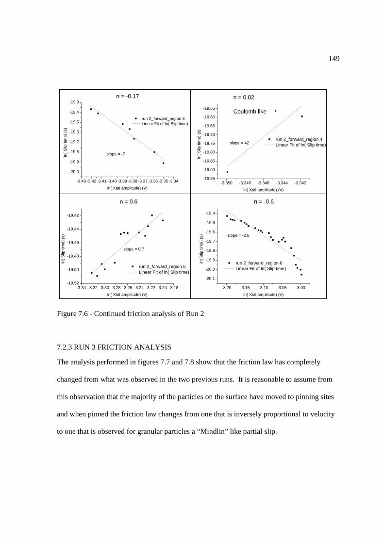
149

Figure 7.6 - Continued friction analysis of Run 2


The analysis performed in figures 7.7 and 7.8 show that the friction law has completely

changed from what was observed in the two previous runs. It is reasonable to assume from

this observation that the majority of the particles on the surface have moved to pinning sites

and when pinned the friction law changes from one that is inversely proportional to velocity

to one that is observed for granular particles a “Mindlin” like partial slip.

-3.43 -3.42 -3.41 -3.40 -3.39 -3.38 -3.37 -3.36 -3.35 -3.34

-20.0

-19.9

-19.8

-19.7

-19.6

-19.5

-19.4

-19.3


ln(

Slip

tim

e) (

s)


slope = -7

n = -0.17

-3.350 -3.348 -3.346 -3.344 -3.342-19.95

-19.90

-19.85

-19.80

-19.75

-19.70

-19.65

-19.60

-19.55


ln(

Slip

tim

e) (

s)


slope = 42

n = 0.02

Coulomb like

-3.34 -3.32 -3.30 -3.28 -3.26 -3.24 -3.22 -3.20 -3.18-19.52

-19.50

-19.48

-19.46

-19.44

-19.42


ln(

Slip

tim

e) (

s)


slope = 0.7

n = 0.6

-3.20 -3.15 -3.10 -3.05 -3.00

-20.1

-20.0

-19.9

-19.8

-19.7

-19.6

-19.5

-19.4


ln(

Slip

tim

e) (

s)


slope = -2.6

n = -0.6

150

Figure 7.7 -Friction analysis of Run 3

0.015 0.020 0.025 0.030 0.035 0.040 0.045 0.0507999894

7999896

7999898

7999900

7999902

7999904

7999906 run 3_forward run 3_backward

Fre

quen

cy (

Hz)

Xtal Amplitude (V)

0.015 0.020 0.025 0.030 0.035 0.040 0.045 0.050-182

-180

-178

-176

-174

-172

-170

-168

region 6

region 2

region 5

region 3

region 4

Df

Df (

Hz)

Xtal Amplitude (V)

region 1

-3.95 -3.90 -3.85 -3.80 -3.75 -3.70 -3.65 -3.60 -3.55

-19.15

-19.10

-19.05

-19.00

-18.95

-18.90

-18.85

-18.80


ln(

Slip

tim

e) (

s)


slope = -0.8

n = 5

Mindlin like

-3.55 -3.50 -3.45 -3.40 -3.35

-19.30

-19.28

-19.26

-19.24

-19.22

-19.20

-19.18

-19.16

-19.14


ln(

Slip

tim

e) (

s)


slope = -0.56

n = 2.3

Mindlin like

151

Figure 7.8 - Continued friction analysis of Run 3


AQUEOUS SOLUTION IN HORIZONTAL ORIENTATION AFTER

INTENTIONALLY DISRUPTING SURFACE BY INDUCING PARTICLE

MOTION.

No motion was observed for the decoupling curves studied in section 7.2. In order to

generate motion on the surface the sample was connected to a separate oscillator circuit that

was tuned to output a larger voltage. When doing so significant motion was observed with

-3.35 -3.34 -3.33 -3.32 -3.31 -3.30

-19.30

-19.25

-19.20

-19.15

-19.10

-19.05

ln(

Slip

tim

e) (

s)



slope = 9

n = 0.1

Coulomb like

-3.30 -3.29 -3.28 -3.27 -3.26 -3.25 -3.24-19.13

-19.12

-19.11

-19.10

-19.09

-19.08

-19.07

-19.06

-19.05

-19.04


ln(

Slip

tim

e) (

s)


slope = 1.3

n = 0.4

Coulomb like

-3.26 -3.24 -3.22 -3.20 -3.18 -3.16 -3.14 -3.12

-19.048

-19.046

-19.044

-19.042

-19.040

-19.038

-19.036

-19.034

-19.032

-19.030

-19.028


ln(

Slip

tim

e) (

s)


slope = 0.1

n = 0.9

viscous like

-3.12 -3.10 -3.08 -3.06 -3.04 -3.02

-19.14

-19.12

-19.10

-19.08

-19.06

-19.04


ln(

Slip

tim

e) (

s)


Slope = -0.96

n = 25

Mindlin like

152

fraction of spheres leaving the surface. Once the motion generation experiment was

complete the sample was connected back on the original electronics to perform additional

decoupling curves. The aim was to observe the effect shaking and depinning of the particles

would have on the decoupling curves. We found that system as indicated by figures 7.9 and

7.10 moved into the weak coupling regime of the Dybwad model. This was an interesting

find but, not a complete surprise since particles of this size (15 microns) have been observed

in the literature4 to fall in to the intermediate coupling regime of the Dybwad model.

Detailed friction analysis was not performed for this experiment since our method requires

that the particles are in the strong coupling regime of the Dybwad model as discussed in

chapter 3 of this thesis.

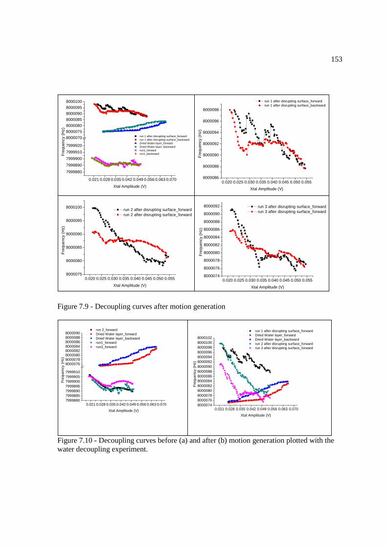
153

Figure 7.9 - Decoupling curves after motion generation

Figure 7.10 - Decoupling curves before (a) and after (b) motion generation plotted with the water decoupling experiment.

0.021 0.028 0.035 0.042 0.049 0.056 0.063 0.070

7999880

7999890

7999900

7999910

7999920

8000070

8000075

8000080

8000085

8000090

8000095

8000100

run 1 after disrupting surface_forward run 1 after disrupting surface_backward Dried Water layer_forward Dried Water layer_backward run1_forward run1_backwardF

requ

ency

(H

z)

Xtal Amplitude (V)0.020 0.025 0.030 0.035 0.040 0.045 0.050 0.055

8000086

8000088

8000090

8000092

8000094

8000096

8000098

run 1 after disrupting surface_forward run 1 after disrupting surface_backward

Fre

quen

cy (

Hz)

Xtal Amplitude (V)

0.020 0.025 0.030 0.035 0.040 0.045 0.050 0.0558000075

8000080

8000085

8000090

8000095

8000100 run 2 after disrupting surface_forward run 2 after disrupting surface_forward

Fre

quen

cy (

Hz)

Xtal Amplitude (V)0.020 0.025 0.030 0.035 0.040 0.045 0.050 0.055

8000074

8000076

8000078

8000080

8000082

8000084

8000086

8000088

8000090

8000092 run 3 after disrupting surface_forward run 3 after disrupting surface_forward

Fre

quen

cy (

Hz)

Xtal Amplitude (V)

0.021 0.028 0.035 0.042 0.049 0.056 0.063 0.070800007480000768000078800008080000828000084800008680000888000090800009280000948000096800009880001008000102

run 1 after disrupting surface_forward Dried Water layer_forward Dried Water layer_backward run 2 after disrupting surface_forward run 3 after disrupting surface_forward

Fre

quen

cy (

Hz)

Xtal Amplitude (V)

0.021 0.028 0.035 0.042 0.049 0.056 0.063 0.0707999880799988579998907999895799990079999057999910

80000768000078800008080000828000084800008680000888000090

run 2_forward Dried Water layer_forward Dried Water layer_backward run1_forward run3_forward

Fre

quen

cy (

Hz)

Xtal Amplitude (V)

154


AQUEOUS SOLUTION IN VERTICAL ORIENTATION AFTER

INTENTIONALLY DISRUPTING SURFACE BY INDUCING PARTICLE

MOTION.

After performing a the third decoupling curve run in the experiment shown in figure 7.9 the

sample was rotated into the vertical orientation (parallel with gravity) with oscillation

direction perpendicular with gravity (VH orientation). When performing the first decoupling

curve an immediate change in the surface behavior was observed as suggested by the

direction of the decoupling curve. The transition for horizontal orientation to the vertical

orientation moved the particles further into the weak regime as indicated by the rise in

frequency from the horizontal runs studied in figure 7.9 to the vertical runs shown in figure

7.11. This observation provides strong evidence that the acceleration of gravity has an

observable affect on the decoupling behavior of microparticles (15 micron in this case)

during QCM experiments. After the initial varied behavior in the decoupling curve observed

in run 1 the decoupling trend returned to what was observed in the previous experiment

performed in the horizontal orientation.

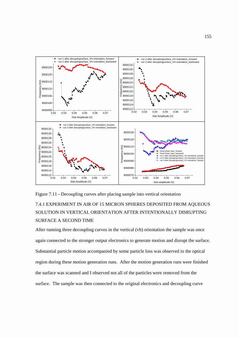
155

Figure 7.11 - Decoupling curves after placing sample into vertical orientation

7.4.1 EXPERIMENT IN AIR OF 15 MICRON SPHERES DEPOSITED FROM AQUEOUS

SOLUTION IN VERTICAL ORIENTATION AFTER INTENTIONALLY DISRUPTING

SURFACE A SECOND TIME

After running three decoupling curves in the vertical (vh) orientation the sample was once

again connected to the stronger output electronics to generate motion and disrupt the surface.

Substantial particle motion accompanied by some particle loss was observed in the optical

region during these motion generation runs. After the motion generation runs were finished

the surface was scanned and I observed not all of the particles were removed from the

surface. The sample was then connected to the original electronics and decoupling curve

0.02 0.03 0.04 0.05 0.06 0.078000095

8000100

8000105

8000110

8000115

8000120

8000125

run 1 after disruptingsurface_VH orientation_forward run 1 after disruptingsurface_VH orientation_backward

Fre

quen

cy (

Hz)

Xtal Amplitude (V)

0.02 0.03 0.04 0.05 0.06 0.078000112

8000114

8000116

8000118

8000120

8000122

8000124

8000126

8000128

8000130

8000132


Fre

quen

cy (

Hz)

Xtal Amplitude (V)

0.02 0.03 0.04 0.05 0.06 0.078000112

8000114

8000116

8000118

8000120

8000122

8000124

8000126

8000128

8000130

8000132


Fre

quen

cy (

Hz)

Xtal Amplitude (V)

0.02 0.03 0.04 0.05 0.06 0.078000070

8000080

8000090

8000100

8000110

8000120

8000130

Dried Water layer_forward Dried Water layer_backward run 1 after disruptingsurface_VH orientation_forward run 2 after disruptingsurface_VH orientation_forward run 3 after disruptingsurface_VH orientation_forward

Fre

quen

cy (

Hz)

Xtal amplitude (V)

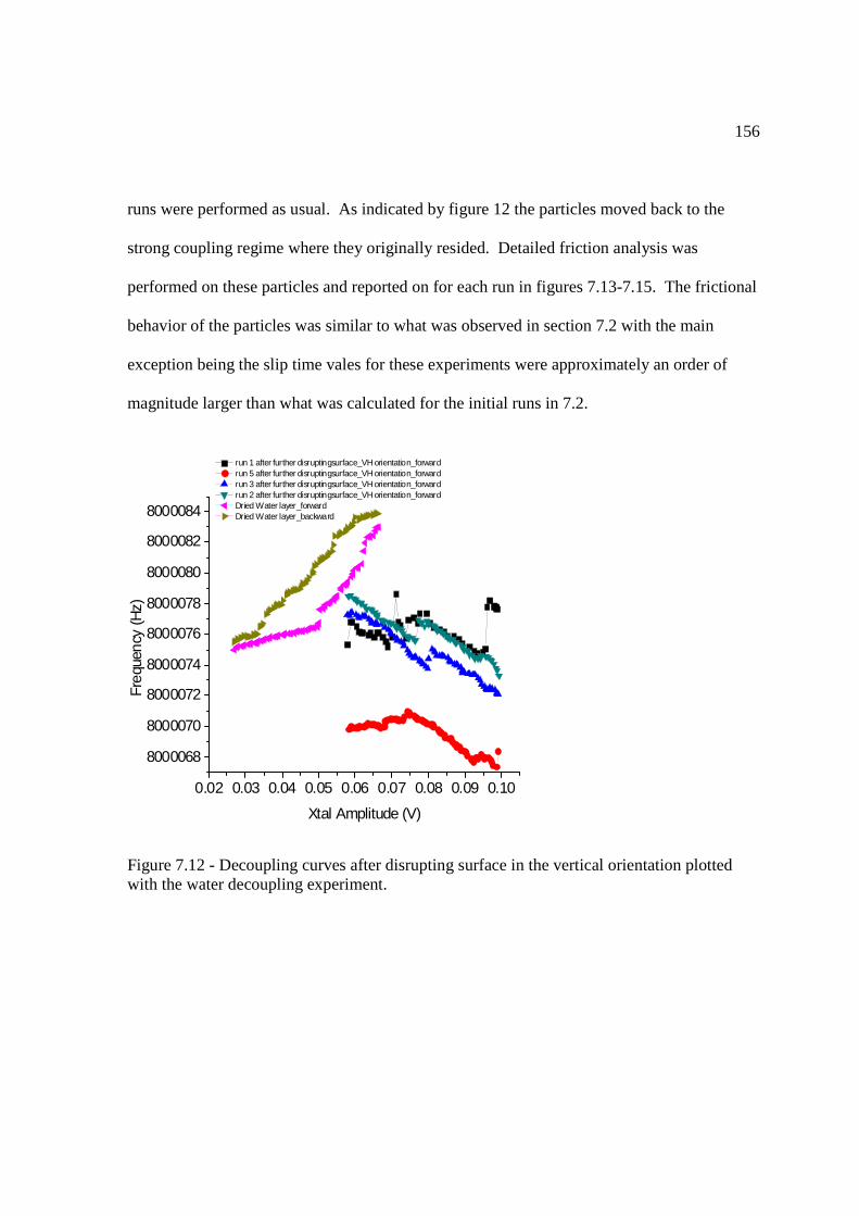
156

runs were performed as usual. As indicated by figure 12 the particles moved back to the

strong coupling regime where they originally resided. Detailed friction analysis was

performed on these particles and reported on for each run in figures 7.13-7.15. The frictional

behavior of the particles was similar to what was observed in section 7.2 with the main

exception being the slip time vales for these experiments were approximately an order of

magnitude larger than what was calculated for the initial runs in 7.2.

0.02 0.03 0.04 0.05 0.06 0.07 0.08 0.09 0.10

8000068

8000070

8000072

8000074

8000076

8000078

8000080

8000082

8000084

run 1 after further disruptingsurface_VH orientation_forward run 5 after further disruptingsurface_VH orientation_forward run 3 after further disruptingsurface_VH orientation_forward run 2 after further disruptingsurface_VH orientation_forward Dried Water layer_forward Dried Water layer_backward

Freq

uenc

y (H

z)

Xtal Amplitude (V)

Figure 7.12 - Decoupling curves after disrupting surface in the vertical orientation plotted with the water decoupling experiment.

157

7.4.2 FRICTION ANALYSIS OF RUN 1

Figure 7.13 - Friction analysis of first decoupling curve run after disrupting surface in the vertical orientation.

0.05 0.06 0.07 0.08 0.09 0.108000074.5

8000075.0

8000075.5

8000076.0

8000076.5

8000077.0

8000077.5

8000078.0

8000078.5

8000079.0

8000079.5

run 1 after further disruptingsurface_VH orientation_forward run 1 after further disruptingsurface_VH orientation_backward

Fre

quen

cy (

Hz)

Voltage (V)

-2.9 -2.8 -2.7 -2.6 -2.5 -2.4 -2.3-16.6

-16.4

-16.2

-16.0

-15.8

-15.6

run 1 after further disruptingsurface_VH orientation_forward Linear Fit of ln( Slip time)

ln(

Slip

tim

e) (

s)ln( Xtal amplitude) (V)

slope = -1.2

n = -5

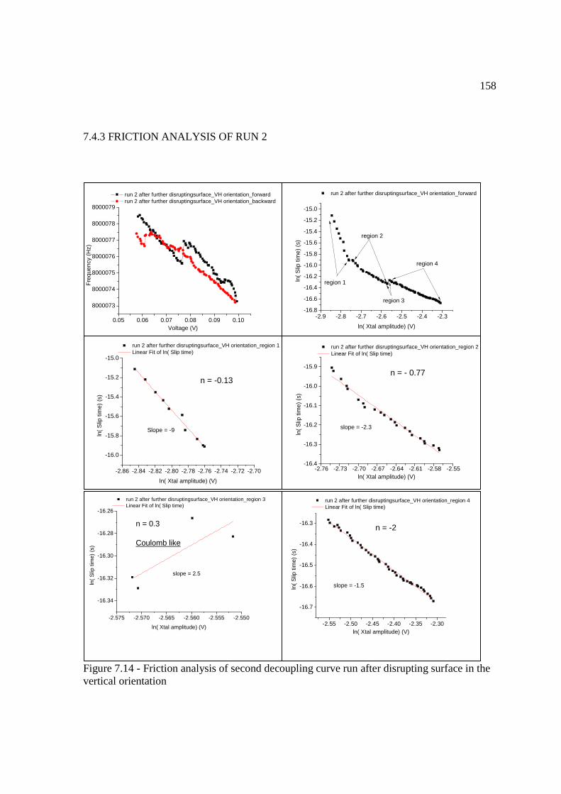
158


Figure 7.14 - Friction analysis of second decoupling curve run after disrupting surface in the vertical orientation

-2.9 -2.8 -2.7 -2.6 -2.5 -2.4 -2.3-16.8

-16.6

-16.4

-16.2

-16.0

-15.8

-15.6

-15.4

-15.2

-15.0

run 2 after further disruptingsurface_VH orientation_forward

ln(

Slip

tim

e) (

s)


region 1

region 2

region 3

region 4

0.05 0.06 0.07 0.08 0.09 0.10

8000073

8000074

8000075

8000076

8000077

8000078

8000079


Fre

quen

cy (

Hz)

Voltage (V)

-2.86 -2.84 -2.82 -2.80 -2.78 -2.76 -2.74 -2.72 -2.70

-16.0

-15.8

-15.6

-15.4

-15.2

-15.0

run 2 after further disruptingsurface_VH orientation_region 1 Linear Fit of ln( Slip time)

ln(

Slip

tim

e) (

s)


Slope = -9

n = -0.13

-2.76 -2.73 -2.70 -2.67 -2.64 -2.61 -2.58 -2.55-16.4

-16.3

-16.2

-16.1

-16.0

-15.9


ln(

Slip

tim

e) (

s)


slope = -2.3

n = - 0.77

-2.575 -2.570 -2.565 -2.560 -2.555 -2.550

-16.34

-16.32

-16.30

-16.28

-16.26


ln(

Slip

tim

e) (

s)


slope = 2.5

n = 0.3

Coulomb like

-2.55 -2.50 -2.45 -2.40 -2.35 -2.30

-16.7

-16.6

-16.5

-16.4

-16.3


ln(

Slip

tim

e) (

s)


slope = -1.5

n = -2

159


Figure 7.15 - Friction analysis of fifth decoupling curve run after disrupting surface in the vertical orientation

7.5 VARIATION IN MICROPARTICLE COUPLING AS A FUNCTION OF

TIME

From the previous sections above I have shown several examples of how the friction

associated with 15 micron polystyrene spheres varies with substrate velocity (xtal amplitude).

In the sections that follow data is reported on for microspheres at “constant” (velocity is not

truly constant since the direction is changing with each oscillation of the QCM) substrate

velocity (xtal amplitude). The data from sections 7.5.1 and 7.5.2 show the behavior of the

microspheres in different environments and deposited it different ways. The experiment

shown in 7.5.1 was deposited in the usual way from aqueous solution however, the

experiment shown in figure 7.5.2 was deposited via transfer experiment as described in

detail in chapters 2 and 6. In both experiments slow changes in coupling (frequency) were

0.05 0.06 0.07 0.08 0.09 0.108000067.0

8000067.5

8000068.0

8000068.5

8000069.0

8000069.5

8000070.0

8000070.5

8000071.0

8000071.5

8000072.0

8000072.5


Fre

quen

cy (

Hz)

Xtal Amplitude (V)-2.9 -2.8 -2.7 -2.6 -2.5 -2.4 -2.3

-16.8

-16.7

-16.6

-16.5

-16.4

-16.3

-16.2

run 5 after further disruptingsurface_VH orientation_forward Linear Fit of ln( Slip time)

ln(

Slip

tim

e) (

s)


slope = -0.99

n = 100

Mindlin Slip

160

observed for both experiments. The frequency of occurrence for these varying coupling

events where similar for both experiments (30-40 minutes) but the main difference was the

shape of these events. The sample deposited from aqueous solution (wet deposition) in

figure 7.16 displayed jagged stick-slip like events similar to what was observed during the

decoupling curve runs in the earlier sections. The dry deposition sample figure 7.17 displays

a smooth roughly sinusoidal response with a frequency of about 30 minutes. Figure 7.18

shows the first decoupling curve run after several frequency response curves were performed.

This decoupling curve run demonstrated of a single sphere supports the statement that

particles of this size are in the intermediate coupling regime. The details concerning these

observed slow coupling changes is currently not well understood. It was suggested in a

previous study4 that QCMs may not be the best devices for generating Mindlin microslip

processes. If the observed behavior coupling behavior is Mindlin in nature it is indeed

possible that the observed long periods in coupling changes is a reflection of the QCM

measurement device coupled with friction at the sphere flat contact region. During

decoupling curve runs the surface particles are experiencing additional forces from the

varying oscillation amplitude of the QCM which would aid in initiating the “micro-slip”

mechanism. According to our previous decoupling curve experiments (sections 7.2-7.4) the

observed slipping mechanism or force law for these fixed crystal amplitude experiments is

more than likely a force law that is inversely proportional to velocity.

161

7.5.1 15 MICRON SPHERES DEPOSITED FROM AQUEOUS SOLUTION IN AIR

0 2000 4000 6000 8000 10000

8000570

8000580

8000590

8000600

8000610

8000620

Freq

uenc

y (H

z)

Time (sec)

Frequency (Hz)

xtal amp = 50 mV

"Stick-slip" events are on the order of 30 - 40 minutes

Figure 7.16 - Frequency response over time of a different sample of 15 micron spheres deposited from aqueous solution.

162

7.5.2 SINGLE 15 MICRON SPHERE CAUGHT DURING TRANSFER EXPERIMENT IN

7E-2 TORR VACUUM ENVIRONMENT IN HORIZONTAL ORIENTATION

0 1000 2000 3000 4000 5000 6000 7000

45.0

45.5

46.0

46.5

47.0

47.5

48.0

Fre

quen

cy-7

9949

00 (

Hz)

Time (s)

Frequency-7994900

Period oscillation between is on the order of 30 minutes

Single "dry" sphere in 5E-3 torr vacuum environment

Figure 7.17 - Frequency response over time of a single15 micron sphere deposited in vacuum environment.

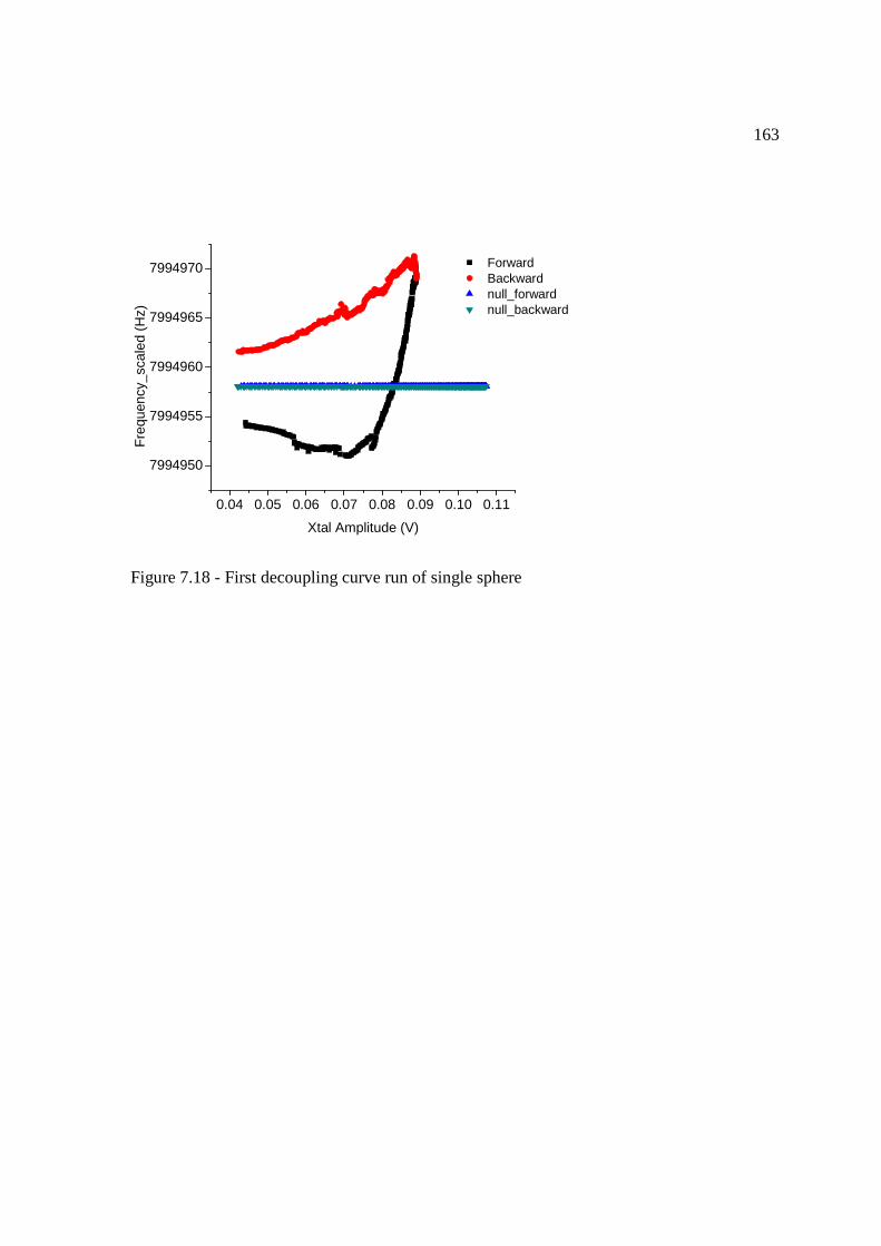
163

0.04 0.05 0.06 0.07 0.08 0.09 0.10 0.11

7994950

7994955

7994960

7994965

7994970 Forward Backward null_forward null_backward

Fre

quen

cy_s

cale

d (H

z)

Xtal Amplitude (V)

Figure 7.18 - First decoupling curve run of single sphere

164

7.6 REFERENCES

1. Dybwad, G. L., A sensitive new method for the determination of adhesive bonding between a particle and a substrate. Journal of Applied Physics 1985, 58 (7), 2789-2789. 2. Sauerbrey, G., Verwendung von Schwingquarzen zur Wägung dünner Schichten und zur Mikrowägung. Zeitschrift für Physik 1959, 155 (2), 206-222. 3. Krim, J.; Watts, E. T.; Digel, J., Slippage of simple liquid films adsorbed on silver and gold substrates. Journal of Vacuum Science & Technology A: Vacuum, Surfaces, and Films 1990, 8 (4), 3417-3420. 4. Vittorias, E.; Kappl, M.; Butt, H.-J.; Johannsmann, D., Studying mechanical microcontacts of fine particles with the quartz crystal microbalance. Powder Technology 2010, 203 (3), 489-502. 5. Etsion, I., Revisiting the Cattaneo--Mindlin Concept of Interfacial Slip in Tangentially Loaded Compliant Bodies. Journal of Tribology 2010, 132 (2), 020801-9.

165

CHAPTER 8: CONCLUSIONS AND FUTURE WORK

8.1 CONCLUSIONS

In this study, methods for interpreting average particle behavior during QCM

experiments have been discussed. We have shown overwhelming evidence that the effects of

water during QCM experiments can not be ignored and in many cases govern the dynamics

as a whole on the surface. The affects of dissipation (bandwidth shift) were not reported on

in this study however, it is important to realize that water will have a huge affect on the

dissipation data especially under a wet decoupling mechanism where large amounts of water

are present. In this study we have found that the analysis of decoupling curves can be quite

complex due to the inconsistent bond strength of the spheres on the surface and the multiple

paths spheres can take once in motion. Due to the nature of the deposition and the sub-

monolayer surface configuration hysteresis and non uniformity can somewhat be expected in

these decoupling curves.

8.2 SUGGESTED FUTURE WORK

A new method was introduced in this thesis for decreasing the presence of water

during QCM experiments and provided sufficient evidence that upon landing the overall

system force of adhesion was greatly reduced and the behavior was reflected in both the

decoupling and delta frequency plots. In the future these experiments should include

dissipation measurements to further support arguments involving the friction mechanism at

the contact. Particle transfer experiments have the potential for many fundamental

166

applications of better understanding the friction mechanism at the microscale. It is possible

with a customized chamber similar to the one I use in this thesis that one could measure the

friction force directly after a transfer experiment. This could be accomplished by catching a

sphere on the target QCM which would be oriented horizontally. Using a camera mounted

directly on the chamber to illuminate the target, one could in principle very carefully rotate

the vacuum chamber (monitoring the angle) and estimate a static coefficient of friction

(assuming pure roll without slip) by angle at which the particle begins to rotate during the

experiment. It is possible that the transfer experiment could be performed multiple times

with in a properly constructed chamber to achieve even drier contacts where surface

dynamics could be probed in a more controlled environment. The notion of micro particle

sorting as suggested by the observed particle motion is not a straight forward task especially

in humid/wet environments. However, it may be easier to achieve such control and sorting in

a dry environment such as particles on the surface after a transfer experiment. Future work

must be done to see if movement can be better controlled and understood.

thesis draft for etd edited - ncsu

Documents