thermodynamic and economic evaluation of existing and prospective processes … · ·...
TRANSCRIPT

DISSERTATION
ThermodynamicandEconomicEvaluationofExistingandProspectiveProcessesfor
LiquefactionofNaturalGasinMalaysia
M.Sc.MohdNazriBinOmar
Berlin


ThermodynamicandEconomic
EvaluationonExistingandPerspectiveProcessesforLiquefactionofNaturalGasinMalaysia
vorgelegt von
Master of Science in Global Production Engineering
Mohd Nazri Bin Omar geb. in Johor Bahru,
Malaysia
von der Fakultät III – Prozesswissenschaften
der Technischen Universität Berlin
zur Erlangung des akademischen Grades
Doktor der Ingenieurwissenschaften
– Dr.‐Ing. –
genehmigte Dissertation
Promotionsausschuss
Vorsitzender: Prof. Dr.‐Ing. Felix Ziegler
Berichter: Prof. Dr. Tetyana Morozyuk
Berichter: Prof. Dr. Wojciech Stanek
Berichter: Prof. Dr.‐Ing. George Tsatsaronis
Tag der wissenschaftlichen Aussprache: 22. Oktober 2015
Berlin, 2016


1
Foreword
ThisworkhasbeenconductedduringmyleavefromUniversitiMalaysiaPerlis UniMAP asa On‐Study Leave staff of School of Manufacturing Engineering, and hence as a Ph.Dstudent at the )nstitute for Energy Engineering at the Technische Universität Berlin TUBerlin .ThisstudywassponsoredbyUniMAPandbytheMinistryofEducationMalaysiainrefertoscholarship)DKPT BS SkimLatihanAkademikBumiputera SLAB .With this opportunity, ) would like to express my utmost praise and gratitude to theAlmightyAllah,andtothepeoplethatfacilitatedthecompletionofthiswork.)amespeciallygratefultoProfessorTetyanaMorozyuk,whosupervisedthisworkandwasalwayswilling,helpful,creativeandpresent.(ersupportwasthemostimportantmotivatortocompletethiswork.Professor George Tsatsaronis was always patient and willing to assist. (is energy andexcitementbrightenedsomecloudydays!)would like to thankProfessor Stanek for the reviewof this thesis. ) amalso thankful toProfessorZieglerforhiswillingnesstochairmythesisdefense.)amindebtedtothestudentsthatcontributedtothiswork:Adrian(iemann,RobertSelim(ill,MehmetÖzbek,andEmreTopal.And,specialthankstomycolleaguesfromtheinstitutefor the fruitful collaboration, eventfulmeetingsandniceexperiencesgathered.TheywereNidal Abboud, Max Sorgenfrei, Berit Erlach, Wanda Ali Akbar and MehrnoushSarcheshmepoor.FortheprovidedsoftwareAspenPlusofAspenTech,)amgrateful.) truly appreciate the help frommy parents and siblings, my wife and children, andmyextended families.Without their sacrifices, the completion of thisworkwould have beenimpossible.Finally, ) would like to thankmyMalaysian ikhwah, akhowat and all my friends here inGermanyandinMalaysiafortheirunderstanding,supportandencouragement.Only(im,Allah,couldrepayalltheabove‐mentioneddeedsinthisworldandhereafter.Berlin,June MohdNazriBinOmar

2
IfLiving’sSimplyToLive
EvenPigsInJungleLive
IfWorking’sSimplyToWork
EvenMonkeysWork(AMKA[ ]

3
Synopsis
LiquefiedNaturalGas LNG intheenergysectorisseenasarealisticsourceforprovidingcleaner,smalltolargescalefuel,duetotheever‐increasingglobalenvironmentalprotectionandhigh demandof electricity at a competitive rate. )n thiswork, several LNGprocessesexistingandprospectiveonesareanalysedthermodynamicallyandeconomically.Refrigerationtechnologyisimportantinassessingtheconsideredenergyconversionplants.Thedifferentdesignsinprecooling,maincryogenicandsubcoolingcyclesamongtheLNG processes, with various pure‐ and mixed‐refrigerants, added the complexity butsignificant in their evaluations. While energetic analysis provides important informationthatcanleadstoplantgeneralperformance,forexamplefromthecumulativecoolingcurveschart, useful energy and irreversibilities of the system and system components can offerbetterassessment.Thisledtothedevelopmentofexergy‐basedanalyses,inwhichexergyoffuel and product at system and component levels derive their exergy destructions andexergetic efficiencies. )n cold production, physical exergy is split into thermal andmechanical exergies because of the wide range of working pressures and temperatures;betweenthehigh Cdownto‐ Cat theircorrespondingpressures,aswellas theirconditional ambient references. Sensitivity analysis helped against the challenges inobtaining the industrial plants datawhere confidentiality, costly information, and limitedreliable sources are in norm. Thus among the examined processes, themost efficient arethose working with the mixed‐refrigerant technology. The highest exergetic efficiencyamongallanalysedsystemsistheC MRprocessat % . mtpa followedbytheMR‐Xprocessat % . mtpa .EconomicanalysisisapproachedtoseetheLNGsystemsfurther.The main cryogenic multi‐flow heat exchangers remain the highest priced compared toothercriticalcomponentsintheirFixedCapital)nvestments.Thetotalcostsfortheanalysedsystems, from . to . $ bn/mtpa, are in rangewith available literatures consistent forgreenfieldpowerplants.AnewlydesignconceptofLNGprocess,theMR‐X,ispresentedtogetherwithsimilaranalyses.)topensupanewinsight,wheresuchdesignisfeasible,practicalandrealistictovariousclimaticandinfrastructurechallengeswhilehavingefficientandeconomichighLNGproductionstrongtocooperatewiththelatestLNGtechnologiesinthemarket.

Zusammenfassung
In der Energiewirtschaft wird verflüssigtes Erdgas (LNG) weltweit als
umweltfreundlicher Energieträger für Klein- und Großanlagen betrachtet, wobei LNG
zur Deckung des stetig wachsenden Bedarfs an elektrischem Strom geeignet ist. In der
vorliegenden Arbeit werden sowohl bestehende als auch neue Prozesse zur LNG
Produktion thermodynamisch und wirtschaftlich analysiert.
Die analysierten Prozesse unterscheiden sich im Bereich der Vorkühlung, der
kryogenen Hauptkühlung durch Kreisprozesse sowie in der Verwendung verschiedener
Kältemitteln, die aus einem Reinstoff oder einem Stoffgemisch bestehen. Basierend auf
Energieanalysen werden Leistungen in den Anlagen zum Beispiel durch Summenkurven
für die Wärmeübertragung ermittelt. Andererseits werden die Komponenten und
Systeme durch Exergie bewertet. Die damit verbundenen exergiebasierten Analysen
nutzen den exergetischen Aufwand und Nutzen zur Ermittlung der Exergievernichtung
sowie der jeweiligen exergetischen Wirkungsgrade. Für die Erzeugung der notwendigen
Kälteleistung wird die physikalische Exergie in einen mechanischen und thermischen
Anteil unterteilt, da der große Bereich von Druck und Temperatur (142 bis -168°C) die
Umgebungsbedingungen überschreitet. Da Betreiber industrieller Anlagen viele
Betriebsparameter vertraulich behandeln und Veröffentlichungen über zuverlässige
Kostendaten kaum existieren, werden Sensitivitätsanalysen verwendet.
Generell stellten sich Prozesse mit Kältemittelgemischen als effizienter heraus.
Als exergetisch effizienteste Prozesse wurden der C3MR-Prozess mit 33% (4,5 mtpa)
gefolgt vom MR-X-Prozess mit 32% (7,8 mtpa) ermittelt. Zum weiteren Verständnis
wurden Wirtschaftlichkeitsanalysen durchgeführt. Im Besonderen sind die Kosten des
Hauptwärmeübertragers, in dem thermische Energie im kryogenen Temperaturbereich
übertragen wird, am höchsten. Die ermittelten Produktgestehungskosten liegen
zwischen 0,3 und 0,6 $bn/mtpa, was im üblichen Bereich für Neubauanlagen liegt. Unter
anderem wird ein neuer Prozess (MR-X) vorgestellt. Dabei wurde festgestellt, dass dieser
Prozess unter verschiedenen klimatischen und infrastrukturellen Rahmenbedingungen
effizient und wirtschaftlich LNG produziert.

4
Table of Contents
1. Introduction .................................................................................................................................................... 16
1.1. LNG chain ................................................................................................................................................ 18
1.2. LNG processes – global and Malaysian context ...................................................................... 19
2. Literature Review on Malaysian LNG Processes .............................................................................. 23
3. Overview on Energy, Exergy, and Economic Analyses .................................................................. 31
3.1. Energy Analysis .................................................................................................................................... 31
3.2. Exergy Analysis .................................................................................................................................... 33
3.2.1. Software requirements for simulation and exergy calculations ............................ 36
3.3. Economic Analysis .............................................................................................................................. 38
3.3.1. Estimation of Total Capital Investment (TCI) ................................................................ 38
4. Processes of Liquefaction of Natural Gas in Malaysia .................................................................... 44
4.1. Propane Pre-Cooled Mixed-Refrigerant (C3MR) LNG Process......................................... 44
4.1.1. Principle of Operation.............................................................................................................. 44
4.1.2. Simulation and Energy Analysis .......................................................................................... 45
4.1.3. Exergy Analysis .......................................................................................................................... 53
4.1.4. Economic Analysis .................................................................................................................... 54
4.2. AP-XTM LNG Process ........................................................................................................................... 56
4.2.1. Principle of Operation.............................................................................................................. 56
4.2.2. Simulation and Energy Analysis .......................................................................................... 57
4.2.3. Exergy Analysis .......................................................................................................................... 60
4.2.4. Economic Analysis .................................................................................................................... 62
4.3. MR-X LNG Process .............................................................................................................................. 67
4.3.1. Principle of Operation.............................................................................................................. 70
4.3.2. Simulation and Energy Analysis .......................................................................................... 71
4.3.3. Exergy Analysis .......................................................................................................................... 72
4.3.4. Economic Analysis .................................................................................................................... 74
5. Conclusion and Future Works ................................................................................................................. 82
6. References ........................................................................................................................................................ 85

5
Appendix A. Research Contributions ..................................................................................................... 91
Appendix B. Energy and Exergy Analyses – Data, Flow and Results ........................................ 92
B.1 General Information on Liquefaction Processes ................................................................... 93
B.2 System testing using PRICO® process [23,24,32] ................................................................ 99
B.3 C3MR Process [73] ........................................................................................................................... 103
B.4 AP-XTM Process [51]......................................................................................................................... 111
B.5 MR-X Process [56,94] ..................................................................................................................... 124
Appendix C. Economic Analysis Data and Flow – A Study Case on the C3MR Process ... 129
C.1 Purchased Equipment Costs (PEC) Estimates ...................................................................... 130
C.1.1 Heat Exchangers ...................................................................................................................... 131
C.1.2 Dissipative coolers ................................................................................................................. 131
C.1.3 Propane and mixed refrigerant compressors ............................................................. 132
C.1.4 Separators .................................................................................................................................. 133
C.1.5 Valves and mixers ................................................................................................................... 134
C.2 Estimation of Total Capital Investment................................................................................... 136
C.2.1 Calculation of startup costs (SUC) and working capital (WC) ............................. 136
C.2.2 Estimation of allowance for funds used during construction (AFUDC) ........... 138
C.3 Estimation of Operating and Maintenance (O&M) Costs ................................................. 141
C.4 Estimation of the Fuel Costs (FC) .............................................................................................. 142
C.5 Estimation of Revenue Requirements ..................................................................................... 143
C.5.1 Total capital recovery ........................................................................................................... 145
C.5.2 Returns on equity and debt ................................................................................................ 146
C.5.3 Taxes and insurance .............................................................................................................. 147
C.5.4 Fuel, operating and maintenance costs ......................................................................... 147
C.5.5 Total revenue requirement (TRR) ................................................................................... 148
C.5.6 Levelized Costs and the Cost of the Main Product .................................................... 150

6
List of Figures
Fig. 1.1. Global LNG demand [6]. ...................................................................................................................... 16
Fig. 1.2. Comparison of transportation cost [9]. ........................................................................................ 17
Fig. 1.3. The process chain for LNG - from Extraction, Processing and Transport to
Consumption [10]................................................................................................................................................... 18
Fig. 1.4 Liquefaction Capacity by Type of Technology, 2013-2018 [15]. ........................................ 19
Fig. 1.5. Malaysia is located in the Asia Pacific basin, color-coded reference by the IGU.
Modified from [15]. ................................................................................................................................................ 21
Fig. 1.6. The three Malaysian LNG process plants including their corresponding trains are
located in Bintulu, Sarawak, an eastern state of Malaysia [17]. .......................................................... 21
Fig. 3.1. A Single Cycle Liquefaction Process [60]. .................................................................................... 31
Fig. 3.2. High level view of refrigeration cycles within processes [60]. ........................................... 32
Fig. 4.1. A general schematic of the C3MR process. .................................................................................. 45
Fig. 4.2. Overall cooling curves for the simulated C3MR process [73]. ............................................ 50
Fig. 4.3. A similar curves for propane pre-cooled MR cycle versus the natural gas’ proposed
by Madhavan [81]. .................................................................................................................................................. 51
Fig. 4.4. Exergy destruction (MW) and exergy destruction ratio (%) for selected components
of the AP-X process. ............................................................................................................................................... 61
Fig. 4.5. Exergetic efficiency for selected components of the AP-X process. .................................. 62
Fig. 4.6. The estimation of direct costs for AP-X process ....................................................................... 65
Fig. 4.7. A general cooling curve for cascade type of LNG process. The smoother curve is the
NG-LNG curve and below it is the refrigerants curve [92]. ................................................................... 67
Fig. 4.8. Cooling curves for C3MR process [92]. ......................................................................................... 68
Fig. 4.9. Exergy destruction (MW) and exergy destruction ratio (%) for the components of
the MR-X process. ................................................................................................................................................... 73
Fig. 4.10. Exergetic efficiency of selected components of the MR-X process. ................................ 73
Fig. 4.11. PEC ($ mil) for selected components of the MR-X process and distribution of the
PEC among the components............................................................................................................................... 76
Fig. 4.12. Levelized total revenue requirement for the MR-X process using different
assumptions for the economic analysis: OMC as a function of CC - between 1% and 10% and
cost of the electricity – between 0.05 and 0.20 $/kWh. ......................................................................... 79

7
Fig. 4.13. Cost per unit of mass of the liquefaction process when different assumptions for
the economic analysis are used. ...................................................................................................................... 80
Fig. B.1. Classification of natural gas liquefaction processes [93]. .................................................... 93
Fig. B.2. A typical coil-wound MCHE for a C3MR process-based LNG plant [103]. .................... 98
Fig. B.3. Flow diagram of PRICO process: CM1 - Compressor 1; COL - Cooler; CM2 -
Compressor 2; CD - Condenser; HE - Heat exchanger; TV - Throttling Valve [24]. .................... 99
Fig. B.4. C3MR flowsheet using Aspen Plus [73]. .................................................................................... 105
Fig. B.5. A general schematic on the AP-X process. ................................................................................ 111
Fig. B.6. Flowsheet for AP-XTM process. ...................................................................................................... 112
Fig. B.7. �- T diagram for HEX0 (∆ ����ℎ = 0.3�).............................................................................. 113
Fig. B.8. �- T diagram for HEX1 (∆ ����ℎ = 6.4�) ............................................................................. 113
Fig. B.9. �- T diagram for HEX2 (∆ ����ℎ = 2.1�).............................................................................. 114
Fig. B.10. �- T diagram for HEX3 (∆ ����ℎ = 17.7�) ........................................................................ 114
Fig. B.11. PETRONAS FLNG to be commissioned in 2015 [15]. ........................................................ 123
Fig. B.12. A general schematic on the MR-X process. ............................................................................ 124
Fig. B.13 Process flow diagram for MR-X process .................................................................................. 125
Fig. B.14. Cumulative cooling curves for the MR-X process. .............................................................. 126

8
List of Tables
Table 1.1. Pounds of Air Pollutant Produced per Billion Btu of Energy [8] ................................... 17
Table 1.2. Typical LNG Compositions at Different Plant Locations [16]. ........................................ 20
Table 3.1. Elements of total capital investment [62]. .............................................................................. 39
Table 4.1. Estimation on Purchased Equipment Cost for selected AP-X process equipments
........................................................................................................................................................................................ 64
Table 4.2. The optimum composition of precooling refrigerants for DMR process analysed by
[93]. .............................................................................................................................................................................. 69
Table 4.3. Estimation of the fixed-capital investment. ............................................................................ 77
Table B.1. Malaysian LNG Plants. ..................................................................................................................... 94
Table B.2. Liquefaction Plants with specific LNG Technology, sorted by year of project start
[102]. ............................................................................................................................................................................ 95
Table B.3. Composition and concentration of natural gas and refrigerants. ................................. 99
Table B.4. Thermodynamic data for material streams at real operating conditions............... 100
Table B.5. Reference values for the exergetic analysis (state 0) for material streams. .......... 100
Table B.6. Detailed thermodynamic data of each chemical component in the streams within
mixed refrigerant. ................................................................................................................................................ 101
Table B.7. Definition of the exergy of fuel and the exergy of product for the components of
the PRICO® process. .......................................................................................................................................... 101
Table B.8. Results obtained from the exergetic analysis. .................................................................... 102
Table B.9. Composition for the C3MR process mixed-refrigerant in molar percentage. ....... 103
Table B.10. LMR and HMR compositions. .................................................................................................. 103
Table B.11. Boiling temperatures (in C) for refrigerants at different pressures [104]. ......... 103
Table B.12. Stream 7 molar fraction and its partial pressures ......................................................... 103
Table B.13. Enthalpy and Entropy Values Required for Exergy Calculation............................... 104
Table B.14. Thermodynamic data for the material streams at real operating conditions for
C3MR process [73]. ............................................................................................................................................. 106
Table B.15. Standard Molar Chemical Exergy Values for Selected Substances at Tref =
298.15K. Model II is referred. ......................................................................................................................... 107
Table B.16. Chemical exergy result for affected streams for C3MR ................................................ 107

9
Table B.17. Definition of the exergy of fuel and the exergy of product for the components of
the C3MR process. ............................................................................................................................................... 108
Table B.18. Exergy rate of product and fuel for the selected components of the C3MR process
..................................................................................................................................................................................... 110
Table B.19. Composition for the AP-X process in molar percentage. ............................................. 111
Table B.20. Thermodynamic data for the material streams at real operating conditions. ... 115
Table B.21. Mole flow rate of the mixed refrigerant. ............................................................................ 117
Table B.22. Definition of the exergy of fuel and the exergy of product for the selected
components of the AP-X process. .................................................................................................................. 119
Table B.23. Exergy rate of product and fuel for the AP-X process. ................................................. 121
Table B.24. Power net required by AP-X process components. ....................................................... 122
Table B.25. Composition of NG and refrigerants for MR-X process. ............................................... 124
Table B.26. Thermodynamic data for the material streams (at real operating conditions). 127
Table C.1. Parameters and assumptions used in TRR calculations [62] ....................................... 130
Table C.2. U and A values of the liquefaction heat exchangers [101]. ............................................ 131
Table C.3. The purchased equipment cost of liquefaction heat exchangers (106$). ................ 131
Table C.4. U and A values of dissipative coolers [106]. ........................................................................ 132
Table C.5. Purchase equipment cost of dissipative coolers (106$). ................................................ 132
Table C.6. The process work input (indicated and net required). ................................................... 133
Table C.7. The purchased equipment cost of the compressors (106 $). ........................................ 133
Table C.8 Sizing parameters of the separators. ....................................................................................... 134
Table C.9 Purchased equipment cost of separators (106$). ............................................................... 134
Table C.10 Purchased equipment cost of throttling valves (106$). ................................................. 135
Table C.11. Estimation of the total capital investment. ....................................................................... 137
Table C.12. The calculated values for the allowance for funds used during construction (106
$). ................................................................................................................................................................................ 139
Table C.13. Statutory percentages for use in the MACRS for a life period of 15 years, annual
tax depreciation and tax book at the end of each year for the LNG plant. ................................... 140
Table C.14. Year-by-year revenue requirement breakdown of the LNG liquefaction plant (106
$) ................................................................................................................................................................ ................. 144
Table C.15. Year by year capital recovery schedule for the LNG plant. (106 $) .......................... 146
Table C.16. Distribution of capital recovery for the LNG plant (106 $). ........................................ 149
Table C.17. LNG plant data set [98]. ............................................................................................................. 152

10
Table C.18. Economic data for the selected LNG plants [98]. ............................................................ 153

11
Nomenclature
Abbreviations
AC aftercooler
AFUDC allowance for funds used during construction
APCI Air Products and Chemicals Inc.
bn billion
C3MR propane pre-cooled mixed refrigerant cycle
CD condenser
CEPCI chemical engineering plant cost index
CI cost index
COMP compressor
COP coefficient of performance
CWHE coil wound heat exchanger
DMR dual mixed refrigerant cycle
EV evaporator
EXP expander
FCI fixed capital investment
FLNG floating liquefied natural gas
HEX pre-cooling heat exchanger
HEX heat exchanger
HMR heavy mixed refrigerant
HPN2 high pressure nitrogen compressor
IC intercooler
LMR light mixed refrigerant
LNG liquefied natural gas
LPG liquefied petroleum gas
LPMR low pressure mixed-refrigerant compressor
LPN2 low pressure nitrogen compressor

12
MACRS modified accelerated cost recovery system
MBtu million British thermal unit
MCE main cryogenic exchanger
MCHE main cryogenic heat exchanger
mil million
MIX mixer
MLHE main liquefaction heat exchanger
MLNG Malaysian Liquefied Natural Gas plant
mmtpa million metric tonne per annum
MPMR middle pressure mixed-refrigerant compressor
MPN2 middle pressure nitrogen compressor
MR mixed-refrigerant
MT million ton
mtpa million ton per annum
N2 nitrogen
NG natural gas
NGL natural gas liquids
PEC purchased equipment cost
PETRONAS Petroliam Nasional Berhad
PFHE plate fin heat exchanger
PHX pre-cooling heat exchanger
PMR parallel mixed refrigerant cycle
PPHE perforated plate heat exchanger
SEPA separator
SMR Single Mixed-Refrigerant
SRK Soave-Redlich-Kwong
TCI total capital investment
TV throttling valve
VALVE throttling valve

13
Symbols
A heat transfer surface area [m2]
C cost rate associated with exergy transfer [$/h]
c cost per unit of exergy [$/GJ]
E time rate of exergy transfer [kW]
e specific exergy [kJ/kg]
F future value of money [$]
f exergoeconomic factor [%]
H rate of enthalpy [kW]
h specific enthalpy [kJ/kg]
ieff effective annual discount rate [%]
k variable used in levelized cost calculations [-]
m mass flow rate [kg/s]
n number of time period [year]
Q heat transfer rate [kW]
p pressure [bar]
P present value of money [$]
r relative cost difference [-]
S rate of entropy [kW/K]
s specific entropy [kJ/kgK]
t income tax rate [%]
T temperature [K, ⁰C]
U overall heat transfer coefficient [W/m2K]
V volume [m3]
v specific volume [m3/kg]
W work [MJ]
W work rate [MW]
X variable represents the size of equipment [-]
Dy exergy destruction ratio [%]
Ly exergy loss ratio [%]

14
Z non-exergy related cost rate [$/h]
Greek letters
α capacity exponent [-] Δ difference [-] ε exergetic efficiency [-]
mechη mechanical efficiency [%]
isη isentropic efficiency [%]
δ variable used for cost difference in coolers [-]
γ activity coefficient [-] τ average annual plant operation hours [h]
Subscripts
BM bare module
ce common equity
CM compressor machine
d debt
D exergy destruction
F fuel
e outlet stream
el electricity
i specified state
i inlet stream
is isentropic
j stream of matter : year
k component of the plant
L levelized value : exergy loss
M material factor
mech mechanical

15
NG natural gas
out exiting exergy
OTXI other taxes and insurance
P product : pressure
PH physical exergy
ps preferred stock
r real escalation
ref reference state
tot overall system
x type of financing
0 ambient/environment state
1-2 control volume inlet and outlet
Superscripts
CH chemical exergy
CI capital investment
KN kinetic energy
M mechanical exergy or cost
OM operating and maintenance
PH physical exergy
PT potential exergy
T thermal exergy
TOT total cost of the stream

16
1. Introduction
Energy worldwide is in demand exponentially [2,3] and expectably will increase even
speedier in the near future while oil reserves are depleting and alternative sources are cost-
challenging. Furthermore, the world’s desire for cleaner type of fuel with numerous
governments regulating environmental policies and incentives for green technologies has
pushed natural gas as an exciting solution.
Natural gas is not new in providing solutions to mankind, as a record shows the
Chinese have applied it commercially some 2 400 years ago [4] and was highly consumed
during the post Second World War. Such abundant source is now providing 23% of the
world’s total energy supply. Its applications currently include but not limited to electricity
generation, grid heating as well as domestic needs. The liquefied natural gas (LNG) is an
enhanced type of such energy, yielding approximately 40% more heating value than any
liquid fuel derived from the chemical conversion of natural gas [5]. In February 2015 BP
showed as per Fig. 1.1 the current and projected global demand for LNG.
Fig. 1.1. Global LNG demand [6].
Among characteristics of LNG are odorless, colorless, shapeless, and lighter than air.
These are advantageous when compared to the solid coal or the liquid oil, especially on the
aspect of greenhouse gas emission (where oil and coal produced 1.4 – 1.75 times more of
CO2), as compiled in Table 1.1. Since January the 1st, the Europeans has had recently
regulated stricter emission control under the International Convention for the Prevention of
1 . I n t r o d u c t i o n
17
Pollution from ships (MARPOL), referring to Sulphur Oxides (SOx) pollution. Thus, LNG-
fueled vessel has become a preferable option due to its low sulphur emission [7].
Table 1.1. Pounds of Air Pollutant Produced per Billion Btu of Energy [8]
Pollutant Natural Gasa Oilb Coalc
Carbon
117 000 164 000 208 000
Carbon
40 33 208
Nitrogen
92 448 457
Sulphur
0.6 1 122 2 591
Particulates 7.0 8.4 2 744
Formaldehyde 0.750 0.220 0.221
Mercury 0.000 0.007 0.016
a Natural gas burned in uncontrolled residential gas burners.
b Oil is # 6 fuel oil at 6.287 million Btu per barrel and 1.03% sulphur
with no post-combustion removal of pollutants. c Bituminous coal at 12,027 Btu per pound and 1.64% sulphur with
no post-combustion removal of pollutants.
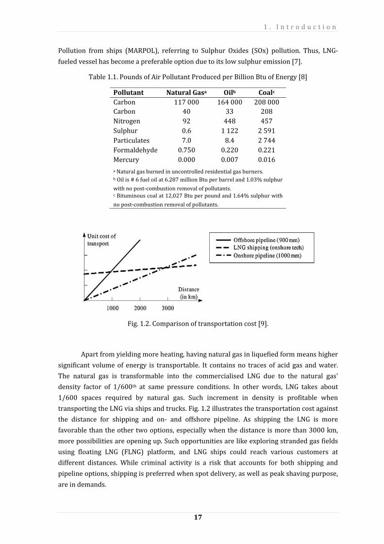
Fig. 1.2. Comparison of transportation cost [9].
Apart from yielding more heating, having natural gas in liquefied form means higher
significant volume of energy is transportable. It contains no traces of acid gas and water.
The natural gas is transformable into the commercialised LNG due to the natural gas’
density factor of 1/600th at same pressure conditions. In other words, LNG takes about
1/600 spaces required by natural gas. Such increment in density is profitable when
transporting the LNG via ships and trucks. Fig. 1.2 illustrates the transportation cost against
the distance for shipping and on- and offshore pipeline. As shipping the LNG is more
favorable than the other two options, especially when the distance is more than 3000 km,
more possibilities are opening up. Such opportunities are like exploring stranded gas fields
using floating LNG (FLNG) platform, and LNG ships could reach various customers at
different distances. While criminal activity is a risk that accounts for both shipping and
pipeline options, shipping is preferred when spot delivery, as well as peak shaving purpose,
are in demands.

1 . I n t r o d u c t i o n
18
1.1. LNG chain
LNG liquefaction and transportation (ship or truck) become economically reasonable when
the reserves size justifies the principal investment of an LNG process plant [4]. The
liquefaction process refrigerates in a particular plant; either peak shaving plant or baseload
plant depending on factors for example customer demand, reserves location, geographical
and economic challenges as well as political conditions. Storage applications are essential
prior to LNG transport and when receiving it for regasification (for sale). Fig. 1.3 shows the
LNG production chain.
Fig. 1.3. The process chain for LNG - from Extraction, Processing and Transport to
Consumption [10]
In the above process chain, after being pointed by geo-exploration team, the raw
natural gas is drill-extracted from its reserves in the earth. The raw gas is firstly fed into a
purification part of the liquefaction plant to remove unwanted materials. Treating the gas is
important to ensure it has as much methane as possible, and contaminants do not interfere
in the process of achieving the optimum temperature for LNG (at about -162 C). Treated
natural gas then enters into the main liquefying phase of the plant. Depending on the
installed refrigeration technology of plant, in modern system the natural gas undergone a
typical pre-cooling by selected refrigerant(s) before proceeds to main cryogenic heat
exchanger (MCHE) for a deeper liquefying and before being sub-cooled. Once the conditions
(pressure and temperature) are met, the liquefied natural gas is kept in storage due to be
shipped at designated times. The LNG ship that will carry the LNG is designed specially,
particularly its tanks, to cater the behaviors of natural gas such as boil-off and regasification
during transport. Based on contracts, the LNG is transported to worldwide customers at
mutually agreed prices. The transported LNG is then being stored before it is regasified into
commercial gas for various needs. Japan, for example, has been among the biggest world’s
LNG importer which Malaysia are among its trusted exporters for the past decades.
Energy Information Administration [11] has reported the costs throughout the LNG
chain in detailed, however, in brief:

1 . I n t r o d u c t i o n
19
• Production of natural gas. The cost of carrying (including all related processing)
natural gas from the reserves to the LNG process plant is 15-20% of the total cost.
• LNG process plant. The cost for all related processes (treatment, liquefaction, by-
production, storage and ship-loading) is 30-45% of the total cost.
• Shipment of LNG. The shipping cost for LNG is 10-30% of the total cost.
• LNG receiving terminal. The cost for all related processes (ship-unloading, storage,
regasification and sales) is 15-25% of the total cost.
The liquefaction plant part of the LNG production chain takes the highest value compared to
the other parts. Among the factors contributing to such cost are the strict design and safety
standards as well as the remote location aspect. Jenson estimated (personal
communication) a base case LNG project particularly on liquefaction part is about $350
million in CAPEX (for a greenfield infrastructure plus $250 million/ton of LNG capacity) and
about $0.20/mmBtu in OPEX [12]. Referring to an Indonesian LNG facility [13,14], the cost
for three trains used to treat and liquefy LNG is $202 million from the total $869 million of
CAPEX, the highest cost contributor comparing to other project components. As such, the
selection of liquefaction technology is the most critical in the whole LNG chain. Proper
classification of the liquefaction technology or process is imperative to ensure the desired
LNG process plant is sustaining as long as possible. Fig. B.1 (Appendix 1) shows a general
classification of natural gas liquefaction processes.
1.2. LNG processes – global and Malaysian context
Fig. 1.4 Liquefaction Capacity by Type of Technology, 2013-2018 [15].
There are at least nine different LNG processes operating around the world. Technologists
are striving in giving better solutions to the increasing demand for better quality of LNG

1 . I n t r o d u c t i o n
20
product while at the same time cheaper and long-lasting. Such efficiency is rapidly seen in
patents and in the industrial world hence competition to achieve higher efficiency of LNG is
inevitable. Fig. 1.4 describes the liquefaction capacity made and forecasted versus the type
of LNG processes.
It can be seen that several processes, such as the APC C3MR/Split MR process and
ConocoPhillips Optimized Cascade process are expected to increase in capacity per year,
whereas others are anticipated to be stagnant and decreasing over the years. These may be
contributed by the increment of LNG production capacity (C3MR/Split MR and Optimized
Cascade), and by the emergence of new LNG process namely Floating LNG process.
Individual processes are decreasing per world’s percentage capacity due to stagnancy. This,
for example refers to the 51% to 38% (estimated) LNG capacity for Air Products’ C3MR
process, in which it will still stay at about 150 mtpa for the next four years to come. The
various kinds of LNG processes provide higher chances for clients (gasfield owner) to have
the best technology that suits their conditions and limitations.
Among the challenges gasfield and process owners are facing are the different
compositions of natural gas extracted. Other components of natural gas may be processed
into commercial by-products, like butane and propane gases. Nevertheless, the lesser these
elements contained in the natural gas the higher percentage of methane gas, and
consequently the cheaper it is for treatment and fractionation, as well as higher volume of
LNG could be produced for sales. Specific processes are necessary to handle the light and
heavy hydrocarbons. The final LNG product, therefore, has different compositions when
compared to other locations. Table 1.2 shows such typical comparison.
Table 1.2. Typical LNG Compositions at Different Plant Locations [16].
Component,
mole %
Das Island,
Abu Dhabi
Whitnell
Bay,
Australia
Bintulu,
Malaysia
Arun,
Indonesia
Lumut,
Brunei
Bontang,
Indonesia
Ras
Laffan,
Qatar
Methane 87.10 87.80 91.20 89.20 89.40 90.60 89.60
Ethane 11.40 8.30 4.28 8.58 6.30 6.00 6.25
Propane 1.27 2.98 2.87 1.67 2.80 2.48 2.19
Butane 0.141 0.875 1.36 0.511 1.30 0.82 1.07
Pentane 0.001 - 0.01 0.02 - 0.01 0.04
The different of LNG composition can be associated with the respective basins namely
Atlantic-Mediterranean basin, Middle East basin and Pacific basin (Fig. 1.5). From Table 1.2,
Malaysia which has the highest methane percentage is located within the Pacific basin.
1 . I n t r o d u c t i o n
21
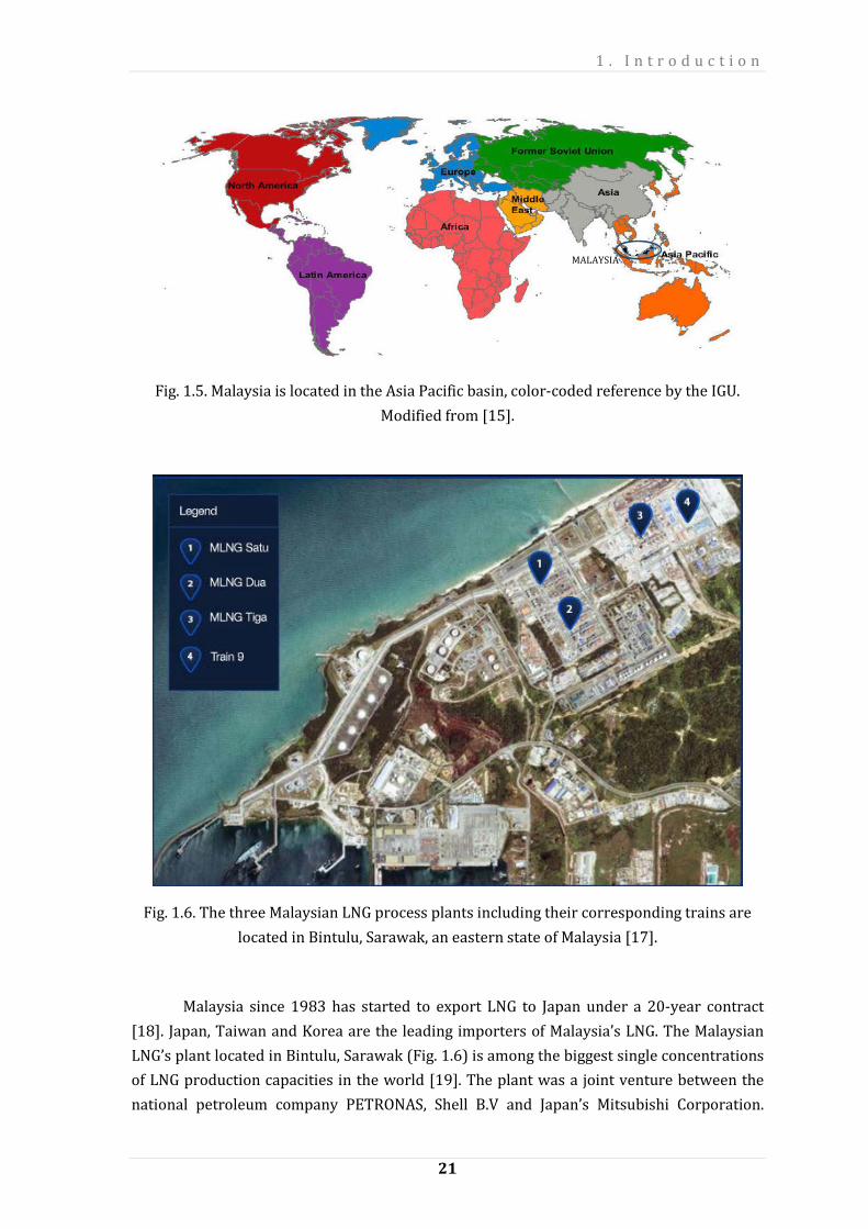
Fig. 1.5. Malaysia is located in the Asia Pacific basin, color-coded reference by the IGU.
Modified from [15].
Fig. 1.6. The three Malaysian LNG process plants including their corresponding trains are
located in Bintulu, Sarawak, an eastern state of Malaysia [17].
Malaysia since 1983 has started to export LNG to Japan under a 20-year contract
[18]. Japan, Taiwan and Korea are the leading importers of Malaysia’s LNG. The Malaysian
LNG’s plant located in Bintulu, Sarawak (Fig. 1.6) is among the biggest single concentrations
of LNG production capacities in the world [19]. The plant was a joint venture between the
national petroleum company PETRONAS, Shell B.V and Japan’s Mitsubishi Corporation.
MALAYSIA

1 . I n t r o d u c t i o n
22
Several characteristics of Malaysian LNG plants are illustrated in Table B.1. As PETRONAS is
expecting their ninth onshore production train completion (adding 3.6 mtpa in capacity),
their PFLNG 1 and 2, built in South Korea, will start producing LNG in 2015 and 2018,
respectively. These will make the global petroleum conglomerate the first company in the
world to bring an FLNG facility to the market. The PFLNG1 will operate at the Kanowit field
offshore Sarawak, and the PFLNG2 will run in the Rotan field offshore Sabah, Malaysia
[20,21]. Both plants will increase Malaysia’s total LNG production capacity from 25.7 mtpa
to 26.9 mtpa and is expected to rise to over 30 mtpa in total by 2017. The industry players
are paying full attention to see how the world’s first Malaysia’s PFLNGs and their
technologies will perform.
23
2. Literature Review on Malaysian
LNG Processes
There are not many specific studies involving MLNG processes which are openly accessible
and at the same time reputable. Although there are numerous publications pertaining to the
market state of MLNG, technical reports about its liquefaction processes are limited.
Following Fig. B.1, a classical cascade type of liquefaction of natural gas is one of the
first LNG processes. It is a three-cascade refrigeration system with single refrigerant for
each cascade. Beside several publications exist in 1960s, this process has been examined by
Morosuk et al. [22] in view of Malaysian operating and environmental conditions. The
analysis includes up to advanced exergetic analysis to reveal the interactions among system
components. The advanced analysis also aided the authors to show potential for improving
the components and overall system thermodynamic efficiencies. Three-cascade
refrigeration system is used. The selection of cascade type of LNG plant may not represent
accurately the existing MLNG plants, but provides bases for a proper and reliable flow of
analyses and methodologies. It is also advantageous for understanding the liquefaction
process system and their process equipment, using explicit EES simulation software, and for
learning necessary assumptions and system boundaries for analyses. Important and less
important liquefaction equipment (for improvement) were found based on their exergy
destructions and exergetic efficiencies. Three components were established as the most
important components for improvements (compressors CM1, CM2, and heat exchangers
CD1-EV1, CD2-EV2). Summarily, conventional exergetic analysis provides useful
information but an advanced exergetic analysis makes such information more precise,
useful and supplies additional information that cannot be supplied by the conventional
analysis. The advanced exergetic analysis is also able to correct the ranking of a certain
component that was initially found from the conventional analysis result (throttling valves
TV2 and TV3). Only CH4 is used as the composition for natural gas thus creates potential for
further improvement where one may replace such composition with a more mixed-type of
natural gas, such as presented in this thesis. The mixture of several components in a gas, or
in a refrigerant, proves, however, more complicated for analyses and, therefore, requires
careful selection of simulation software, data sources, and results interpretations. Apart
from the single-material NG composition, other initial data and assumptions are in the range
of existing MLNG plants data. Among valuable data that validates and support this thesis

2 . L i t e r a t u r e R e v i e w o n M a l a y s i a n L N G P r o c e s s e s
24
data are the outlet temperature for cooling water, the exergetic efficiency and the system
coefficient of performance.
An insight over a type of LNG process called Single Mixed Refrigerant (SMR) is
necessary. This is because the current process for MLNG plants is among the close
successors to the SMR process. Experiences learned from the plants that used the single-
cycle SMR process helped technologists to develop the two-cycle C3MR process. PRICO is a
popular process that uses SMR technology. This process has been drawn up by the
Black&Veatch Company, and the industrial applications of PRICO started in the year 1955,
when it was applied to one of the first world’s LNG plants [23–25]. Three U.S./international
patents cover the PRICO process. At present at least 21 LNG plants use this process while 16
more plants are in the design and/or construction phase. The PRICO process is famous for
LNG peak-shaving units. In the year 2010, 25% of the LNG plants in the U.S. used this
process. Within two years after that, design and construction for the world's first offshore
LNG project started [25]. The following advantages are associated with the PRICO process
[26]: 1) proven process that achieves the promised performance, 2) relative simple
operation, 3) minimal refrigerant inventory, 4) reduced number of equipment items, 5) low
capital cost and operating cost, 6) high flexibility, 7) high reliability, and 8) rapid startup.
There are not many research publications dealing with liquefaction processes;
however, the PRICO (SMR) process recently became quite popular among researchers. Four
processes for small-scale LNG plants were evaluated by Remeljej and Hoadley, 2006 [27].
The PRICO process was selected there as a reference process. An exergy analysis was
performed in a simple way, and only relative data are given. The exergy destructions
(thermodynamic inefficiencies) are distributed as follows: 21% - within both compressors,
30% - within both coolers, 46% - within a heat exchanger, and 3% - within the throttling
valve. The paper concluded that, among all studied processes, the SMR process has the
lowest exergy consumption for the compressors, and that the main difference between the
processes was caused by efficiency differences of the expander-driven compressors. Jensen
and Skogestad, 2009 [28] discussed eight compositions of the mixed refrigerant that usable
for the PRICO process; the effect of properties of the mixed refrigerant to the main
characteristics of the PRICO process were reported. The authors demonstrated that
increasing the concentration of nitrogen within the mixed refrigerant leads to an
improvement in the heat-transfer performance of all heat exchangers. An application of the
gradient-free optimization-simulation method to processes modeled with the simulator
Aspen HYSYS is reported by Aspelund et al., 2010 [29]. The PRICO process was selected as
an academic example for the optimization for two reasons: firstly, this process is a simple
LNG process with seven independent variables (opted by the authors). This number is too
large for the optimization routine but small enough to be optimized with an optimization-
simulation tool. The second reason is that it is possible to verify the results by investigating
the hot and cold composite curves. The paper focused on the number of iterations required
to get an optimal concentration of the mixed refrigerant. Mokarizadeh Haghighi Shirazi and
Mowla, 2010 [30] discussed the simulation of SMR concepts and the properties that are

2 . L i t e r a t u r e R e v i e w o n M a l a y s i a n L N G P r o c e s s e s
25
used in MATLAB to generate the objective function. A genetic algorithm was used for
optimization. The energy consumption of the process was minimized. Depending on the
concentration of the refrigerant, the specific energy consumption can be reduced from 1485
kJ/kg LNG to 1186.6 kJ/kg LNG or from 1126.7 kJ/kg LNG to 1092.4 kJ/kg LNG. The smaller
values were taking from Lee, 2001 [31] (as a reference publication). The authors applied
also an exergy analysis, in order to calculate the values of the exergy destruction within the
components: 31% - within both compressors, 33% - within both coolers, 27% - within the
heat exchanger, and 9% - within the throttling valve. Hiemann, 2011 [32] conducted a
detailed exergy analysis of the PRICO process. Here the approach “exergy of fuel/exergy of
product” has been used taking into account a splitting of the physical exergy into thermal
and mechanical parts. Marmolejo-Correa and Gundersen, 2012 [33] selected the PRICO
process as an academic example to demonstrate the effect of using different approaches in
the exergy analysis (“inlet exergy/outlet exergy” versus “exergy of fuel/exergy of product”
as well as splitting of the physical exergy into thermal and mechanical parts) on the
obtained results. The authors assumed the operation conditions without necessarily a
reference to real plants. Xu et al., 2013 [34] reported the results of the optimization of the
concentration of the refrigerant as a function of the inlet temperature to the heat exchanger
(263.15 K through 313.15 K). For the optimization, a genetic algorithm coupled with the
process simulation software Aspen Plus has been used. The results show that when the
ambient temperature increases, the concentrations of methane, ethylene and propane
should decrease while the concentration of isopentane should increase. In this way, the
overall exergetic efficiency can be increased from 30% (calculated by the authors for the
commercial concentration of the refrigerant) up to 39.6-42.3%. In this paper, the exergetic
efficiency is a function of COP and of a “correlation factor”. In their follow-up paper, the
effect of concentration on each working fluid within the mixed refrigerant was investigated.
Such is to minimize the specific power consumption (the value of 1003.6 kJ/kg LNG was
reached), i.e. maximize the values of COP and exergetic efficiency. The reported value of
COP=0.782 is surprisingly high in comparison with results reported in other publications;
however, the definition of COP is not given. The exergetic efficiency was calculated as 43.9%,
which is in the range of other available data for the PRICO process. The distribution of the
exergy destruction within the components is as follows: 36% - within both compressors,
27%- within both coolers, 26% - within the heat exchanger, and 11% - within the throttling
valve. Sequential quadratic programming was also applied to the optimization of the PRICO
process (Morin A. et al., 2011) [35]. The research focused on the method used for
optimization. The optimization results related to the liquefaction process itself were
discussed very briefly for the two study cases, in which the mixed refrigerant is with and
without pentane. Through the energetic optimization, the specific energy supply decreases
by 3.12%. Again the same optimization procedure for the PRICO process was reported by
Wahl et al., 2013 [36]. The optimal composition of the mixed refrigerant was a function of
the composition of the natural gas (so-called “lean natural gas” and “rich natural gas”). The
heat-transfer characteristics for the multi-flow heat exchanger are also discussed. The main

2 . L i t e r a t u r e R e v i e w o n M a l a y s i a n L N G P r o c e s s e s
26
goal of the authors was to get the results of the optimization within a short period of
execution time, in comparison with the optimization procedure discussed by Aspelund et al.,
2010 [29] that required 12 h. Castillo and Dorao, 2012 [37], discussed economic issues
related to LNG processes. They reported the application of Decision-Making (using a Genetic
Algorithm binary coding and Nash-GA) for the PRICO process. The LNG markets were also
considered in the optimization of the PRICO process. Only relative economic data are
reported, for example, the cost of the multi-flow heat exchanger is approximately 10-15% of
the total investment cost and the cost associated with the compression process is always the
dominating factor for all approaches used in the optimization. Khan et al., 2012 [38]
discussed the optimal composition of the mixed refrigerant for the SMR process from the
energetic point of view, i.e. through the minimization of energy consumption for the
compression process (from 1600 to 1528 kJ/kg LNG). The log mean temperature difference
within the multi-flow heat exchanger is 7.8 K. The SMR process was modeled in the UniSim
Design simulator, and the model was optimized with nonlinear programming. The exergy
analysis was implemented into the described optimization methodology (Khan et al., 2013
[39]) and more complex mixed refrigerant processes were optimized. Heldt, 2011 [40]
developed and tested a mathematical model for control strategies, in order for the SMR
processes to operate at optimal conditions. High attention was given to the modeling of the
multi-flow heat exchanger based on industrial experimental data. The literature review for
the evaluation of the PRICO (SMR) process shows that mainly energetic optimizations were
discussed using different methods for the mathematical optimization and corresponding
algorithms. Sometimes the selected method for optimization and its
improvement/robustness were more important to the authors that the obtained results
related to the PRICO process. The objective function of the optimization refers mainly to the
composition of the mixed refrigerant. An economic analysis is not very common for the
evaluation of the PRICO liquefaction process. Morosuk et al. [24] reiterated the variety
advantages that PRICO process has, and added that recently it has become popular among
researchers. As the simulated process was a two-staged compression ( =1CMW 44.70 MW
and =2CMW 46.51 MW), the energetic analysis showed among others that 5.6 MW more
would be required if one-stage compression was applied. From their evaluation, the PRICO
process productive components (compressors, heat exchanger and throttling valve) have
high exergetic efficiencies (80-90%). More interesting and useful information can be
obtained on the interdependence between the components and the real potential for their
improvement through advanced exergetic analysis. Conclusively, PRICO, in general, is well-
designed in terms of thermodynamics and economics while its heat exchanger could be
improved further due to the intensiveness of energy, cost, and environmental impact. These
are, after all, common challenges to all LNG process plants. The evolution from a single-cycle
to the two-cycle proved to be significant worldwide as process owners continuously seek
possibilities for higher capacity production. Since 1970s, the SMR process plants with
capacities about 1 mtpa were quickly replaced by the C3MR process [41], with Brunei
Lumut 1 plant as the first utilising the C3MR (in 1972) [42].
2 . L i t e r a t u r e R e v i e w o n M a l a y s i a n L N G P r o c e s s e s
27
The C3MR process was developed for improving the SMR process. The
improvements were cycle efficiency and increasing capacity potential per LNG train. AP
reported [43] that the SMR train at Libya had a capacity of around 0.6 mtpa per train, and
the first C3MR process plant at Brunei is more than 1 mtpa per train of capacity. This
improvement of at least 0.4 mtpa was mostly caused by the reduction in MR volumetric flow
due to the propane pre-cooling configuration. The reduction also effectively debottlenecked
the MCHE and MR compression equipment design. From the experiences gained in the
Brunei Lumut 1 C3MR process as well as in other parts of the world, process developers and
owners with Malaysian Government started the MLNG complex. Kasmuni et al. [44]
reported the historical growth of MLNG Complex. The three plants - MLNG Satu, MLNG Dua,
and MLNG Tiga, and their expansions (1983) are detailed down to the utilities and facilities.
The type and arrangement of coolers, staged-compressors, and cryogenic heat exchangers
are revealed. All three MLNG plants have common C3MR process as their primary LNG
production technology. The authors compared installed components between the C3MR
plants and their advantages and disadvantages. This is because each MLNG plant and train
has a different arrangement of drivers and compressors, different in type of turbines, and
some have been debottlenecked for more production. For example, the plants use a similar
kind of heat exchanger for the Main Cryogenic Heat Exchanger (MCHE) that is of spiral
wound type. However, with different ‘bundle design’ (the MLNG Satu with a 3-bundle design
and the MLNG Dua with 2-bundle design), the former has 4 warm-end feed circuits (NG,
light MR, heavy MR and a low pressure LPG reinjection circuit) and the latter has 3 warm-
end feed circuits. This warm-end feeds help researchers to simulate the MCHE more
accurately in the simulation software. Incorrect match between warm and cold feeds in the
simulation interface results in crossover of the temperature progress for the particular heat
exchanger. Crossover issue prevents simulating system to converge fully. Using the
experiences gained from MLNG Satu and MLNG Dua, MLNG Tiga has the preferred 3-bundle
design with 3 warm-end circuits (warm, middle and cold). Kasmuni et al. also show the
number of propane compression stages that differs between the plants, from 3 stages to 4
stages of compression. The useful information about the (maximum) temperature of
seawater cooling was found. Related economic views are presented, and some challenges
due to the continuous modifications of the MLNG plants are given. The information about
the mixed refrigerant and the reason behind the selection of C3MR process are, however,
unavailable. It may be helpful if the authors also present the different design schematics
between the existing MLNG plants. The schematics should vary from plants to plants over
the past decades of installation, retrofitting and debottlenecking. The starters and turbine
drivers are distinguished as well. MLNG Satu uses the steam turbine to power the
compressors while MLNG Dua and MLNG Tiga use gas turbine driven compressors. The
application of gas turbine on the LNG plants proved better efficiency in fuel and reduced the
complexity, compared to the steam-based plant. This is because the gas turbine is directly
connected to the compressor shaft, and the absence of boilers (steam generation)
equipment, steam cycle water treating water facilities, as well as overall cooling

2 . L i t e r a t u r e R e v i e w o n M a l a y s i a n L N G P r o c e s s e s
28
requirements for the plant, were significantly reduced. While using steam turbine as the
driver has the advantages of high reliability and availability, it may require a large space for
its operation and maintenance [45]. Meanwhile, the intensive maintenance and high CO2
emissions related to the gas turbine are still challenges need to be further improved.
MLNG Satu initially commissioned at a total capacity of 8.1 mtpa, has since de-
bottlenecked to yield a further 30% of its initial capacity. This significant increment was
done using operating experiences at other plants existed at that time, including the Brunei
LNG plant [46]. The steam-based plant is cooled using seawater heat exchangers while
MLNG Dua and MLNG Tiga use hybrid (sea water and air) heat exchangers to cool the gas
turbine based plant.
Awang [47] in the LNG Journal explained the growing challenges of heat exchanger
operations at MLNG plants. Some relevant information for future simulation works is
shown, for example, the detailed components specifications and characteristics. The
methods and modifications of the seawater cooling line were presented. The report focused
mainly on maintenance and inspection especially on the main cryogenic heat exchanger.
Hence, only a few important aspects are significant to this thesis though one may see from
the author’s recommendations the complexity of analysing the internal side of LNG heat
exchangers. Potential for future works from this thesis is seen possible by referring to the
subject of Awang’s report.
Norrazak et al. (1998) [48] define in their report the fundamental features of the
MLNG Tiga project during its development with particular emphasis on the integration
aspects of the previous existing two plants. The particular LNG process is mentioned
together with its cooling and driving types. The train fuel efficiency is claimed to be
enhanced by the use of gas turbine exhaust heat waste, but specific value or percentage of
such efficiency cannot be found. Although stated as simplified, the C3MR process flowsheet
revealed in their paper is comprehensive comparing to other available sources. It is
significant to note the mention of the Main Cryogenic Heat Exchanger (MCHE) that was
supplied by APCI. This confirmation is important because it came from the client itself
(PETRONAS), and, therefore, all data from APCI websites and white papers became more
reliable for reference purpose. There are other MCHEs produced by different cryogenic-
based component companies with various efficiencies and qualities. Norrazak et al. also
confirmed the 4-stage propane precooling compressor (while the previous two plants are 3-
stage precooling compression [44]), and the liquefaction and endflash compressors are
driven by an average specific power of 12.4 kW/tpd (or around 34 MW/tpy), in which they
claimed to be low.
Norrazak et al. (2004) [49] in another paper presented the usage of dynamic
simulation for research of plant design and verification of the plant performance, claiming it
to be effective. The simulation model included a full representation of the propane, mixed
refrigerant and the natural gas circuits. At the particular year mentioned, the MLNG Tiga
trains have been among the largest ever built with an annual capacity of 3.9 mtpa. The type

2 . L i t e r a t u r e R e v i e w o n M a l a y s i a n L N G P r o c e s s e s
29
and number of compressor used in this plant are revealed; (apart from one 4-stage
centrifugal type mentioned above) one low pressure axial type MR compressor and one high
pressure centrifugal type MR compressor (connected both by a common shaft). The
arrangement of compressors and drivers is presented in a schematic. An example of simple
propane refrigeration system was illustrated however this was not part of the MLNG Tiga
plant, but only to show the use of dynamic simulation. From there the compressor
performance was shown. The authors reported in detail on how to simulate a real
complicated system, component by component design and head curves. Interestingly, for
heat exchanger models they used a fixed value for UA in the LMTD calculation. This value
was retrieved through the physical property from their database. The value was not shown
in the report. In estimating the costs for LNG heat exchangers, among important factors are
the UA values. In this paper, several parameters for example MR composition and LP MR
compressor are permitted to be manipulated while others are restricted during the quest of
searching the maximum value LNG production. Among the restrictions are all temperature
approach in the MCHE should be higher than a predetermined minimum, typically 1 or 2
degree Celsius, and compression power must be less than or equal to the maximum
allowable power. This information is valuable for researchers to manipulate parameters
while restricting other variables during software simulation, especially whenever data
availability and reliability are difficult to have or to validate. In the same lengthy report,
Norrazak et al. established a set of steps for verification of system and failure scenario. The
final section may as well be another potential for future works in furthering LNG process
research and development particularly in health, safety and environment aspects.
It is widely known about the C3MR to AP-XTM system evolution, but it is not so for
the AP-XTM to AP-NTM evolution. PETRONAS will be using the latter process in their floating
LNG production entirely soon, and it is worth to understand the AP-XTM first due to the
implication similar to SMR-C3MR process evolution mentioned earlier. The AP-XTM has been
reported significantly only by its investors [26,50] and Omar et al. [51]. In the latter study,
the system was simulated using Aspen Plus and analysed energetically and exergetically in
detail. The AP-XTM used Propane (pre-cooling), MR (liquefying) and Nitrogen (sub-cooling).
The addition of the third cycle (the Nitrogen cycle) is the main evolution from the two-cycle
C3MR process. The process is presented in this thesis after the C3MR process section. While
the COP of the AP-XTM was found to be 0.14, and its overall exergetic efficiency was 15%, the
exergetic efficiency for each component of the system is in between 65% to more than 95%
individually, which is a high percentage range for such type of efficiency. Of the total exergy
destruction, 28% is associated with the main heat exchanger and two multi-stage
compressors. A further evaluation of this process should be conducted, suggested by the
authors, using advanced exergy analysis where the interdependence between the
components as well as the real potential for improving the overall system will be
discovered. AP-XTM so far is claimed by reputable sources to be the largest operating
liquefaction capacity production. Based on such success and experience, the company built
the latest AP-NTM, which has been confirmed for PETRONAS’ FLNG application [21].

2 . L i t e r a t u r e R e v i e w o n M a l a y s i a n L N G P r o c e s s e s
30
The Borneo Post [52] recently reported about the two PETRONAS’ FLNGs (PFLNG)
that will increase the current Malaysia LNG production output of 25.7 mmtpa. The FLNG1
will contribute 1.2 mmtpa and FLNG2 1.5 mmtpa. The FLNG vessels will use AP-NTM
technology [53–55] while Dual-Mixed Refrigerant (DMR) technology is being seen as a
favorite to be integrated into this newest area of LNG production. However, note that the
DMR process was developed for Arctic climate operation conditions - low average annual
temperature but relatively high-temperature differences during the year [56]. Therefore,
the use of mixed refrigerant instead of propane refrigerant as their pre-cooling refrigerant
proved to be critical due to the negative effect of propane, for example when operating
below -30 C. Meanwhile, the AP-NTM which evolved from the AP-XTM, (the former) used only
Nitrogen (which has very low boiling temperature) to liquefy and sub-cool NG. With this,
PETRONAS will be the world pioneer in the LNG production via FLNG. Such move is
expected to transform Malaysia into an ‘LNG import-free nation’ by 2016 [57] as currently
Malaysia regasifies short-term contracted LNG from overseas for domestic usage. The
PFLNG is expected to accommodate the regasification storing capacity of 3.8 mtpa. The
FLNG market is young and has enormous potentials to be explored in terms of process
integration and innovation. It is interesting to explore and design a new concept of
liquefaction of natural gas that could integrate or retrofit C3MR, AP-X, and DMR together, for
better capacity and efficiency. A new design is presented in the final part of this thesis as
MR-X with simulations, analyses and discussions.
Weems and Sullivan [58] in 2014 presented the “LNG at 50 - History and Projected
Future for Liquefied Natural Gas Exports in an Unconventional Era” at an annual meeting of
Rocky Mountain Mineral Law Institute. They set their report based on decades of LNG
history, and Malaysia’s are shown grouped together with Australia, as major LNG exporters.
Classic and on-going contracts are detailed with relations to the U.S. and European markets.
Current and planned LNG technologies are provided, especially the Malaysian floating
storage and regasification vessels (FSRUs). It is expected that the report is not technically
explored due to the wide breadth of scopes covering many countries. Nevertheless, charting
prices of LNG per producing/importing countries for the past 50 years may prove
important, particularly when reduction of capital investment for plant construction is taken
into consideration. The absence of such prices may due to the issue of confidentiality.
Nonetheless, Damon Evans [59] reported some gas prices in which the Malaysian
power producer Tenaga Nasional Berhad (TNB) pays at 4.53 $/mmBtu (or 0.016 $/kWh).
Even though in the process chain the final LNG product is several steps behind the
commercially gas product, the pricing may not be far in range of the said price due to factors
for instance government subsidy, transport distance, and long-term contract incentives.
Lately it is reported that Malaysia is projected to be fully independent of LNG (or rather
having no LNG import at all) in a year thus such condition reduces the risk of global LNG
price volatility [57] at least for Malaysia.

31
3. Overview on Energy, Exergy,
and Economic Analyses
3.1. Energy Analysis
In discussing the LNG technologies used in Malaysia, it is important to understand first the
basics of a liquefaction process. The success of a liquefaction process is influenced much by
the number of cycles it has. An example of a cycle is shown in Fig. 3.1.
Fig. 3.1. A Single Cycle Liquefaction Process [60].
Pre-treated natural gas is fed at warm temperature into the cycle, and the cycle cools
it until it becomes liquefied. For the cycle to have the cooling, Work, � is put into it using
compressor, and heat must be rejected from it using air or water cooler. The compressor
usually has its dedicated working fluid or refrigerant. Hence the compressor (size, type), its
refrigerant (flowrate, composition), and its driver (size, type) that contribute to the amount
of work � are key factors for a cooler LNG in such process.
While there are peak-shaving LNG plants that use single-cycle process, almost all
base-load LNG plants use either two- or three-cycle process. For example, the widely used
Propane Pre-Cooled Mixed Refrigerant (C3MR) process has two cycles; the first is the
Propane cycle that pre-cools feed gas and mixed-refrigerant, and the second is the mixed-
refrigerant cycle that cools and sub-cools up to the final product. Each of this cycle has their
own refrigerant, compressors and heat exchangers.
Among existing LNG processes that use three cycles are AP-XTM, Linde MFC, and the
ConocoPhillips Optimized Cascade (refer Table B.2 for all existing LNG processes). Fig. 3.2
shows the macro level view of refrigeration cycles within processes.

3 . O v e r v i e w o n E n e r g y , E x e r g y , a n d E c o n o m i c A n a l y s e s
32
Fig. 3.2. High level view of refrigeration cycles within processes [60].
This thesis discusses in detail the two-cycle process (C3MR) and three-cycle process
(AP-X and MR-X) only, through software simulations and their analyses that follow.

3 . O v e r v i e w o n E n e r g y , E x e r g y , a n d E c o n o m i c A n a l y s e s
33
3.2. Exergy Analysis
Exergy is the maximum theoretical useful work (shaft work or electrical work) obtainable
from a thermal system as it brought into thermodynamic equilibrium with the environment
while interacting with the environment only [61]. The environment is a large equilibrium
system, in which the state variables (T0, p0) and the chemical potential of the chemical
components contained in it remain constant, when, in a thermodynamic process, heat and
materials are exchanged between another system and the environment. It is important that
no chemical reactions can take place between the environmental chemical components. The
environment is free of irreversibilities and the exergy of its amounts to zero. In any thermal
system surroundings, the environment is part of the surroundings.
For an energy conversion system, the total exergy can be divided into four main
parts (neglecting nuclear, magnetic, electrical and surface tension effects): physical,
chemical, kinetic and potential exergy [62], that is ���� = ������ + � � + � � + ��� (3.1)
The rate of physical exergy ������ associated with a material stream (subscript j) is ��� = �� − � � − � − � (3.2)
where � and denote the rates of enthalpy and entropy, respectively. The subscript 0
denotes values at temperature and � of the environment. The physical exergy, where
similarly ��� = � ∙ �� (3.3)
= �� �ℎ − ℎ � − ∗ �� − � � �. At per unit kilogram of mass, the physical exergy of a working fluid can be further
split into its thermal (eT – due to its temperature) and mechanical (eM – due to its pressure)
exergy components: �� = � + (3.4)
�� = ��ℎ − ℎ ,�� − (� − � ,���=�����.+ ��ℎ ,� − ℎ , � − (� ,� − � , ��0=�����.
(3.5)
where X is the state where the temperature is at ambient temperature, and the pressure is at
specified temperature, or specifically [62]

3 . O v e r v i e w o n E n e r g y , E x e r g y , a n d E c o n o m i c A n a l y s e s
34
�� = ��ℎ − ℎ @�0,��� − �� − � @�0,��� �
+ ��ℎ @�0,�� − ℎ @�0,�0� − �� @�0,�� − � @�0,�0� � (3.6)
Exergy destruction � , and exergy loss � , are measures of inefficiencies
associated with the irreversible processes taking place in k-th system component. Exergy
analysis additionally often involves the calculation of measures of performance: exergy
destruction ratios, exergy loss ratio and exergetic efficiencies. As dimensionless criteria are
used for performance evaluations, an appropriate defined exergetic efficiency
unambiguously characterizes the performance of a system or system component from the
thermodynamic viewpoint. The rate of exergy destruction in the kth component is given by � , = � , − ��, − � , (3.7)
Here, � , represents the exergy loss in kth component, which is usually zero when the
component boundaries are at . For the overall system, � includes the exergy flow rates of
all streams leaving the system.
Exergy of product, �� is the desired result expressed in exergy terms, and achieved
by the system (the k-th component) being considered. �� is defined to be equal to the sum
of:
• all the exergy values to be accounted at the outlet (including the exergy of energy
streams generated in the component) plus
• all the exergy increases between inlet and outlet (i.e. the exergy additions to the
respective material streams) that are in accord with the purpose of the component.
Exergy of fuel, � is the exergetic resources expended to generate the exergy of the
product. Similarly, � is defined to be equal to:
• all the exergy values to be accounted at the inlet (including the exergy of energy
streams supplied to the component) plus
• all the exergy decreases between inlet and outlet (i.e. the exergy removals from the
respective material streams) minus
• all the exergy increases (between inlet and outlet) that are not in accord with the
purpose of the component.
The performance evaluation and the design optimization of thermal systems require
a proper definition of the exergetic efficiency and an appropriate costing approach for each
component of the system. The exergetic efficiency of a component and fuel are defined by
��
��

3 . O v e r v i e w o n E n e r g y , E x e r g y , a n d E c o n o m i c A n a l y s e s
35
considering the desired result produced by the component and the resources expended to
generate the result. � =�,��,� = 1 − �,� �,� (3.8)
In addition to � and � , , the thermodynamic evaluation of a system component is
based on the exergy destruction ratio , , which compares the exergy destruction in the
kth component with the fuel supplied to the overall system � ,��� :
y =� ,� ,���
(3.9)
This ratio expresses the percentage of the decrease in the overall system exergetic efficiency
due to the exergy destruction in the kth system component:
� =��,���� ,��� = 1−� , − � ,���� ,���
(3.10)
����� =��,���� ,���
(3.11)
� , is an absolute measure of the inefficiencies in the kth component, whereas � and ,
are relative measures of the same inefficiencies. In � the exergy destruction within a
component is related to the fuel for the same component, whereas in , the exergy
destruction in a component is related to the fuel for the overall system.
Alternatively, the component exergy destruction rate can be compared to the total exergy
destruction rate within the system, � ,��� , giving ratio
∗ =� ,� ,���
(3.12)
For the comparison of dissimilar components, the exergy destruction ratio may be
used. The exergy loss ratio can be defined similarly, by comparing the exergy loss to the
exergy of the fuel provided to the overall system:
=� ,���� ,���
(3.13)
Where and when necessary, chemical exergy is considered as referred to the
correlation in equation (3.1). The tabulated values for standard molar chemical exergy for
substances at normal environment conditions [61], help chemical exergy calculation. Such
calculation, for an ideal mixture of N ideal gasses,
�� ��������� ������ = � � ∗��= � � + � ∗ ∗� � ∗�
�= ln ( �) (3.14)

3 . O v e r v i e w o n E n e r g y , E x e r g y , a n d E c o n o m i c A n a l y s e s
36
and, for liquids (where coefficients of activity, �� is involved),
��������� = � � ∗��= � � + � ∗ ∗� � ∗�
�= ln (γ� ∗ �) (3.15)
The coefficients of activity, �� is represented as ‘gamma’ in Aspen Plus. Aspen Plus also
checked the enthalpy balances. Most components had zero error, while the maximum error
among components was in the scale of around 10-12 W. There are two models for the
tabulated standard chemical exergy values: The first one is suggested by [63] and uses pref =
1.019 atm, while the second one is suggested by [64] and uses pref = 1 atm [65]. The second
model was used because for this system pref was also taken as 1 atm.
3.2.1. Software requirements for simulation and exergy calculations
Aspen Plus [66] simulates LNG process system, components and streams. To prepare for
simulation, the following are the necessary inputs:
1. Components – Specifications: All involved materials must be identified here,
depending on the desired system to be simulated.
2. Methods – Specifications – Global – Property methods & options – Base method: SRK
(Soave-Redlich-Kwong). The Methods Assistant helps to suggest user to choose
property method based on user’s input [67].
3. Methods – Specifications – Global – Petroleum calculation options – Free-water
method: STEAMNBS. This method is selected due to its correlation with the SRK
method above.
4. Methods – Specifications – Global – Referenced – Reference methods: PENG-ROB,
CHAO-SEA, PSRK, REFPROP, RK-SOAVE, RKSWS, SRK, SR-POLAR. These are chosen
based on their specific approach towards natural gas, mixtures and non-ideal system
equation of state.
5. Property Sets – Properties: GAMMA. This property is chosen only when chemical
exergy is concern, where it is referred as the activity coefficient, �� [68]. It is strongly
recommended to remove this property should chemical exergy is not considered to
avoid multiple error messages in the Aspen Plus’ Control Panel.
To calculate the two split exergies, �� and � to have more accurate physical
exergy, the equation (3.6) could be executed using common formulas in Microsoft Excel
spreadsheet [69]. However, the spreadsheet requires from Aspen Plus unit-customized
results of each stream’s:
i. mass enthalpy (J/Kg), ℎ
ii. mass enthalpy (J/Kg), ℎ @�0,�� iii. mass enthalpy (J/Kg), ℎ @�0,�0
iv. mass entropy (J/Kg.K), �

3 . O v e r v i e w o n E n e r g y , E x e r g y , a n d E c o n o m i c A n a l y s e s
37
v. mass entropy (J/Kg.K), � @�0,�� vi. mass entropy (J/Kg.K), � @�0,�0
vii. mass flow (Kg/s), �
viii. ambient temperature (K),
Hence the calculated thermal and mechanical parts are in Watts units. As ��� = �� + � (3.16)
the addition of both results should produce the physical exergy. This could be validated
using physical exergy result produced from Fortran-Aspen subroutines calculations in
Megawatts (MW) term. Such MW term is useful for the next step calculation – exergies for
fuel and product of system and system components.
3 . O v e r v i e w o n E n e r g y , E x e r g y , a n d E c o n o m i c A n a l y s e s
38
3.3. Economic Analysis
An important aspect of analysing a process is economy. The success of a process design is
always, but not limited to, measured by monetary terms. To accomplish such, a complete
design of a process relies on the estimation of costs – of major things for example important
equipment, capital investment including fuel, operation and maintenance, and the
estimation of the final cost of the product. With proper cost estimations through the project
design, important basis for decision making can be achieved.
An initial practical economic analysis is conducted by means of engineering
economics with the help of several assumptions and estimations, in view of the type of the
process, technological and legal environments [29, 32]. For such analysis, it is vital to have
various factors such as the process flow, its flow rates, the process conditions, its
thermodynamic states of each material streams as well as the specifications of necessary
unit operations and equipment. To help the analysis with regards of the said factors, the
Total Revenue Requirement (TRR) method for estimating the Total Capital Investment (TCI)
is referred throughout the economics.
3.3.1. Estimation of Total Capital Investment (TCI)
The TCI of a plant is measured as a one-time cost, unlike cost of fuel or operating and
maintenance costs that are categorized as the continuous expenses, especially when the
plant’s design, construction and start-up phase is concerned. The criteria of the plant TCI are
shown in Table 3.1.

3 . O v e r v i e w o n E n e r g y , E x e r g y , a n d E c o n o m i c A n a l y s e s
39
Table 3.1. Elements of total capital investment [62].
I. Fixed Capital Investment (FCI)
A. Direct costs (DC)
1. Onsite costs (ONSC)
• Purchased equipment cost (PEC)
• PEC installation (45% of PEC)
• Piping (35% of PEC)
• Instrumentation and control (20 % of PEC)
• Electrical equipment and materials (20% of PEC)
2. Offsite costs (OFSC)
• Land (10% of PEC)
• Civil, structural and architectural work (50% of PEC)
• Service facilities (65% of PEC)
B. Indirect costs (IC)
1. Engineering and supervision (35% of PEC)
2. Construction costs (15% of DC)
3. Contingencies (10% of IC)
II. Other Outlays (OO)
A. Startup costs
B. Working capital
C. Cost of licensing, R&D
D. Allowance for funds used during construction (AFUD)
From the TCI criteria there are two main components
1. Fixed Capital Investment (FCI), and
2. Other Outlays (OO)
The FCI is applied for money needed for land and all necessary constructions,
purchases and installations of facilities and equipment of the plant. This is executed by
assuming the period for such FCI is a zero-time period of design, construction and
installation for the total cost of the plant. Properly the FCI is further divided into direct costs
and indirect costs categories. The former are the costs covering the main permanent
components, labor, materials and other means used throughout the construction,
fabrication and installation of the plant’s fixed facilities. The latter are the costs covering
other remaining expenses including temporary facilities needed for the project [29, 32].
Considering the information provided, the total capital investment is calculated as
OOICDCTCI ++= (3.17)
FCI

3 . O v e r v i e w o n E n e r g y , E x e r g y , a n d E c o n o m i c A n a l y s e s
40
Estimation of purchased equipment cost (PEC)
Estimating PEC is the first step in economic analysis. To do that, the construction materials
and the operating conditions of the process are specified. With as much quality data as
possible, the estimation and calculations implemented here will be better in accuracy and
reliability. Estimating the FCI is best when experience of such in the real industrial scene is
taking into account thus vendor’s quotation of any criterion of cost is valuable. The bigger
the scale of the project, the more important it is to consider advices, consultations or at least
price tags from vendors for costly equipment. Otherwise should manufacturer’s quotation
be unavailable due to confidentiality or whatnot, estimations taken from qualified and
seasoned professionals are preferred. These include calculations done from extensive cost
databases of reliable firms. Then, if the two most preferred options are not obtainable,
perhaps due to time or budget limitations, the purchased equipment cost (PEC) can be also
estimated via available charts in the literature [29].
The charts are usually built using the help of a high volume of data in cost and
design. When parameters necessary to get values from the charts are known, such as heat
exchanger’s heat transfer area or compressor’s power, it is easily possible to study the
charts for the desired cost of the equipment. The charts also allow effects of the equipment
characteristics to be taken into account, for example temperature and pressure. The
equipment base cost (CB) which obtainable from the charts is corrected by having these
effects as factors such as material factor (fm), temperature factor (fT) or pressure factor (fp)
[29]. Furthermore, bare module factors (fBM) can be included as well to the equipment final
module cost of, as shown below.
BMpTmdB fffffCPEC = (3.18)
Normally for stainless steel, fM = 2.5 and for electric motor driver, fD =1. For a compressor,
the base cost, referring to the year 2009 (CEPCI 394) is given by [70] � = exp {7.2223 + 0.80[ln(� )]} (3.19)
Typically, the charts available in the literature are costs log-plotted against the
equipment size, resulting in a straight line across the chart. The line’s slope, α, or the scaling
factor, is used for cost estimation of a specific equipment (CPE,Y) at a certain specific
parameter, for instance size (XY), in the presence of the purchase equipment cost of the same
equipment (CPE,W) at a different size (XW), as shown in the Equation (3.20).
α
W
YWPE,YPE,
X
XCC
= (3.20)
The change in reference year and size could fluctuate the scaling factor α. These two
parameters are searchable in the literature for various types of equipment and sizes. Unless
reliable data is available to be used, α may be assumed as 0.6 commonly known as the six-
tenths rule [29].

3 . O v e r v i e w o n E n e r g y , E x e r g y , a n d E c o n o m i c A n a l y s e s
41
Another key parameter for the economic analysis is the cost index. As the charts may
only have data referring for a specific period of time, all data gained from these charts have
to be carried to the same reference year (in which the year used as a basis for all economic
analysis). The Cost Index (CI), or referable as inflation indicator, is stated as
=
yearoriginal
yearreference
originalyearreference
CI
CI
CostCost (3.21)
The objective of this cost index is to correct the costs for the equipment, supplies, labor and
material for the estimation. The indexes typically referred to are Marshall and Swift (M&S)
Equipment Cost Index which is based on the construction expenses for numerous chemical
process industries, and Chemical Engineering Plant Cost Index (CEPCI), which is based on
the construction expenses for chemical plants [29].
Estimation of direct costs of FCI
There are two core divisions for direct costs as they are a component of FCI. Firstly, there is
the onsite costs (ONSC) and secondly the offsite costs (OFSC). While it is probable to
estimate these divisions through assessments based on the detailed flow diagrams of the
system, a factor method is applied for the rest of the calculations. Factor method is used for
respective component in terms of a percentage of the purchased equipment costs (% of
PEC). These percentage values given for each component are established as a product of an
experience from various plants in the chemical process industry [29].
Purchased equipment installation consists of the costs for the shipping and insurance
to bring equipment from the manufacturer to the site, the unloading, handling, ground
works, supports and labor and all other expenses that are significant to install fully the
equipment. The average value of 45 % may be used if any other information is not provided
[29].
Piping represents the expenses that relate to the material and labor costs required
for the construction of the whole piping grid in the plant. The piping costs 10% to 70% of
the purchased equipment costs.
The instrumentation and control rely heavily upon the intricacy of the purchased
equipment. The higher degree of automation and control are resulting more sophistication
in the equipment design, the more these instrumentation and control then costs. Typically, it
covers around 6-40% of the purchased equipment cost.
Electrical equipment and materials is defined as the expenses related to the
materials, installation and labor for distribution lines, power centers, substations,
emergency control supplies, switch gears and area lightning. Average value of 20% of the
PEC is applicable should the information for such section is unavailable.

3 . O v e r v i e w o n E n e r g y , E x e r g y , a n d E c o n o m i c A n a l y s e s
42
Land for the plant relies highly on the location of the plant. Typically, if need be
around 10% of the PEC is expected to cover such cost.
Service facilities are consisting of but not limited to the utilities (water, electricity,
steam and fuel) supply. For such expenses 65% is accounted from the PEC [29].
Estimation of indirect costs of FCI
The costs associated with supervision, construction and contingencies of the plant are
categorized as the indirect costs (IC).
Engineering and supervision expenses consist of the expense for the complete plant
design, drawings and other necessities such as supervision and inspection, scale models,
administration and procurement, travel and advisor fees. This engineering and supervision
may cost 25-75% of the PEC.
The construction fee itself which usually have the charges for movable facilities and
operations, equipment and tools, personnel home office on-site as well as insurances is
assumable at 15% of the PEC.
Contingencies accounts all uncertainties and risks in the actual costs calculations in
view of changing weather, challenges in transportation and sudden price changes, as well as
work stoppages. Contingencies take 5-20% of the FCI relying on the difficulty, size and
uniqueness of the plant [29].
Other outlays
The charges involved in the working funds, startup investment and allowance for funds used
during construction are referred as Other Outlays. These charges are second part of the total
capital investment (TCI).
Startup costs mostly involve the expenses of equipment, materials and overheads
which are funded only throughout the startup phase of the plant prior to its operation. The
startup costs of a thermal system are representable as a total of the unescalated costs such
as one month of permanent O&M charges, one month of unfixed operating costs calculated
at full load, one week of fuel at full load and 2% of the plant facilities investment.
Additionally, to these outlays, working capital is the capitals needed for the period of
the plant operation. It is essential for the operating costs prior to receiving the payment
from the product sale. Working capital includes the investment for [29]
a) raw materials, fuels and provisions carried in stock
b) finished goods in stock and semi-finished goods in the process of being
manufactured

3 . O v e r v i e w o n E n e r g y , E x e r g y , a n d E c o n o m i c A n a l y s e s
43
c) monies kept on hand for operating expenses, taxes and other current
obligations, and
d) accounts receivable
e) accounts payable
The allowance for funds used during construction (AFUDC) characterizes the time
value of the money through the construction, based on an interest rate equivalent to the
weighted cost of capital. Taking into account the construction period of a plant, portion of
the outlay is necessary to cover design studies, civil, acquisition, engineering effort and
setting up of equipment without having any income from the plant [29].

44
4. Processes of Liquefaction of
Natural Gas in Malaysia
Three LNG processes are discussed here in details: Propane Pre-cooled Mixed-Refrigerant
(C3MR), AP-XTM, and newly-developed MR-X.
The PRICO process however is not discussed in detail because it was used exclusively for
testing the simulation and mathematical models. The testing, executed prior to the three
former-mentioned LNG processes, was necessary to see the possibility (a) to simulate them
in suitable platforms, and (b) to analyse them using energy and exergy analyses especially
when involving the mixed-refrigerant cases. To regard such contributions and their
importance, the PRICO system is shown in Appendix B.1 (System testing using PRICO®
process).
4.1. Propane Pre-Cooled Mixed-Refrigerant (C3MR)
LNG Process
4.1.1. Principle of Operation
To facilitate the understanding of C3MR process, Fig. 4.1 is used for simplification and Fig.
B.4 is used for simulation. Mainly there are two main blocks (or cycles per Fig. 3.2). The first
block is the pre-cooling block, which uses Propane as its refrigerant (refer Legend). The
second block uses mixed-refrigerant to liquefy and successively sub-cool, in the central heat
exchanger known as the Main Cryogenic Heat Exchanger (MCHE) (or sometimes referred as
“coldbox”).

4 . P r o c e s s e s o f L i q u e f a c t i o n o f N a t u r a l G a s i n M a l a y s i a
45
Fig. 4.1. A general schematic of the C3MR process.
Typically, wet natural gas (NG) undergoes the pre-treatment process. In the pre-
treatment process, acid gas is firstly being removed from the NG. It then proceeds to
dehydration (water removal) and mercury removal process. After that, natural gas liquids
(NGL) are withdrawn from the NG. The NGL normally is sent for fractioning various by-
products such as Ethane and LPG among others. The pre-treatment and fractionation
processes for the C3MR process plant, however, are not analysed in detail in this thesis.
At (above) near ambient temperature, the cleaned NG from pre-treatment is fed into
the pre-cooling block at about 65 bar. The mixed-refrigerant coming from the coldbox is also
fed into this pre-cooling block, at about 48 bar. Both feeds’ temperatures produced from this
block are about -33°C. Throughout the cycles (including liquefaction), heat is removed using
air and/or seawater through inter- and after-coolers, to the environment. The pre-cooled
NG is fed into the coldbox to be liquefied and sub-cooled. The MR that received refrigerating
effect from the pre-cooling block is separated into gas and liquid phase through a phase
separator before going into the coldbox, at about 84 kg/s and 218 kg/s respectively, to
liquefy and subsequently sub-cool NG. A typical coldbox for a C3MR process-based LNG
plant is shown in Fig. B.2. The vaporized- and liquid-phase mixed-refrigerants recombine at
the exit (bottom catchment) of the coldbox. It is looped back afterwards into the pre-cooling
block driven by axial compressors [71] of several stages. The sub-cooled NG, which at this
state as liquefied, exits the coldbox. About temperature -162 C and slightly above ambient
pressure, through valve-throttling, the final LNG product, is ready for storage for shipment
purpose. Other targets may be implemented such as recycling flashed LNG into the system,
local electricity sources or further by-products.
4.1.2. Simulation and Energy Analysis
Aspen Plus [66] is chosen to simulate this process. For initialization, the Soave-Redlich-
Kwong (SRK) property method, recommended by the Aspen Property Method Assistant is
selected for this C3MR process simulation. Generally, SRK is recommended for gas
applications, as it can calculate the enthalpy and entropy values of the process streams, it is

4 . P r o c e s s e s o f L i q u e f a c t i o n o f N a t u r a l G a s i n M a l a y s i a
46
appropriate for a mixture of non-polar or mildly-polar, consistent even in the critical region,
and reasonable results can be found at all pressures and temperature [67].
Assumptions and specifications for the process, are as follow:
• The ambient temperature and pressure are set as 25 C (298. 15 K) and 1.01325
bar, respectively.
• Pressure drops throughout all heat exchangers are assumed to be 3% (in side
pipes), and no pressure loss for propane cycle for simplicity sake [22,72].
• It is also assumed no pressure loss within phase separators and mixers, and all
phase separations are specified to have no heating duty.
• The isentropic efficiencies are assumed to be 78% (propane compressors) and
75% (mixed-refrigerant compressors).
• The mechanical efficiencies are assumed to be 90% for all compressors.
• The discharge pressures for propane compressors are specified as 2.5 – 5.1 – 7.2
– 14.3 bar, and for mixed-refrigerant compressors are as 7.5 – 17.5 – 48.6 bar
[73].
• The initial values necessary to simulate NG feed, propane and mixed-refrigerant
mass flows are regulated according to a common LNG train capacity that used
C3MR process, which is at 4.5 mtpa. As such, the propane mass flow is specified
as 442.7 kg/s, the mixed-refrigerant mass flow as 301.8 kg/s, and the NG feed
mass flow is specified as 158.4 kg/s at 65 bar and 300 K (26.85 C)
• The composition for this process is as Table B.9 [74].
• The NG feed gas is pre-treated, pre-dried, and all unwanted materials including
acid gas are assumed to be removed before NG is being fed into the pre-cooling
block.
• The final LNG product is set to be slightly above ambient pressure, 1.2 bar
(113.15 K or -160 C) for further purpose such as storage.
Fig. B.4 shows the detailed C3MR process flowsheet used in the simulation using Aspen Plus.
For this particular simulation, full vapor NG at 65 bar and 26.85 C enters the first
pre-cooling heat exchanger, HEX1 and is pre-cooled by two-phased Propane at 14.19 C
through stream 19. The colder NG (17.85 C) leaves HEX1 and enters another three pre-
cooling heat exchangers HEX2, HEX3, and finally HEX4. Each of them has a similar pre-
cooling arrangement as the first; that is Propane that has been expanded pre-cools NG. NG
exits HEX4 at -33.15 C (57.55 bar) leaving the pre-cooling block and enters the liquefaction
and sub-cooling block through stream 43.
Each of these pre-cooling heat exchangers produces two-phase Propane (stream 20,
23, 26 and 29) which increases in temperature as the stage increases. They are separated
into vapor and liquid state using separators, where the former is used for compression, and
the latter is valve-expanded for pre-cooling. The vaporized Propane exiting from HEX4 is

4 . P r o c e s s e s o f L i q u e f a c t i o n o f N a t u r a l G a s i n M a l a y s i a
47
however recompressed. Such arrangement in series of stages, as the Propane’s pressure
being let down, reduces its temperature further and provides refrigeration to the NG.
Meanwhile in view of the refrigerant, the vaporized Propane is recompressed by
centrifugal compressor COMP1 from 1.3 bar (-34.65 C) to 2.5 bar (-7.73 C). It is then mixed
with separated Propane gas (stream 38 at 2.5 bar and -19.24 C) for the next series of
compression stages. Similar compression arrangement as the first one for the next COMP2,
COMP3 and COMP4. The Propane gas leaves COMP4 and enters its aftercooler at 14.3 bar
and 58.37 C. After expanded, the partially-condensed Propane pre-cools the first pre-cooling
heat exchanger HEX1 through stream 19 (7.2 bar).
For the mixed-refrigerant coming from the liquefaction and sub-cooling blocks into
the pre-cooling block, it enters the first pre-cooling HEX1 at 31.85 C and 48.2 bar. It then
continues to receive the refrigerating effects at all pre-cooling heat exchangers that follow.
The mixed-refrigerant leaves HEX4 at -33.15 C similar to that of NG and enters phase
separator SEPA4 for gas-liquid separation.
NG at gas state enters the liquefaction and sub-cooling block at MCE1. The MCE1 and
MCE2 heat exchangers with its valves and mixers represent the Main Cryogenic Heat
Exchanger (MCHE). The arrangement is as such so that the industrial MCHE flow and the
main reason behind the flow arrangement could be replicated as close as possible,
considering all the limitations that exist. To simulate the industrial MCHE as per its original
structure would be too complex and out of this thesis’ scope. Inside the MCHE, the NG is sent
through a tube circuit where it is liquefied (from vapor to liquid state, in this case at stream
44) and sub-cooled to -139.15 C at the exit of MCE2, by mixed-refrigerant.
The mixed-refrigerant (vapor at stream 8 and liquid at stream 14) coming from the
phase separator SEPA4 enter the MCHE simultaneously at -33.15 C and 42.63 bar. It is found
when the two-phase mixed-refrigerant is split into its individual vapor and liquid streams,
they formed new compositions of mixed-refrigerant. These mixed-refrigerant vapor stream
and mixed-refrigerant liquid stream are called Light Mixed-Refrigerant (LMR) and Heavy
Mixed-Refrigerant (MHR), respectively. Table B.10 [73] shows the newly formed
compositions.
Both streams climb through separate tube circuits where they are liquefied and sub-
cooled [75]. As they are relieved in pressure reducing their temperatures further, they
vaporize and flow downward on the shell side of the MCHE. This provides the liquefaction
(stream 13) and sub-cooling (stream 11) to the NG. Then, exiting the MCHE, the vaporized
mixed-refrigerant is sent to the compressors for recompression.
For the mixed-refrigerant coming from MCHE to be recompressed, a series of axial
compressors is used starting with COMP5 compressing the vaporized mixed-refrigerant
from 2.82 bar (-270.33 C). COMP6 and COMP7 with intercooler further compress it up to
48.6 bar (109.12 C), before being after-cooled and reinserted into the pre-cooling block.

4 . P r o c e s s e s o f L i q u e f a c t i o n o f N a t u r a l G a s i n M a l a y s i a
48
For the final product, LNG at stream 45 (54.15 bar, -139.15 C) is expanded through
VALVE7 and is sent to a high pressure phase separator. Due to the expansion any vaporized
NG is separated into stream 47. The vast expansion expands the LNG down to a slightly-
above ambient pressure (1.22 bar) and further reduces the LNG temperature to -160 C. Such
pressure and temperature is necessary for later processes such as LNG storage for shipping
or local transportation. A selected simulation results for this C3MR process is shown in
Table B.14.
In energetic analysis of the C3MR process, it is crucial to analyse the flow of energy
conversion process occurred in the particular system.
In the pre-treatment process for example, apart from bulk components such as
water and CO2, hydrogen sulphide, carbon dioxide and mercaptans are also removed from
the NG to ensure the NG that will be inserted into the liquefaction block has heavier
hydrocarbon components [76]. These heavy hydrocarbon components allow them to freeze
at very low temperature, condense, and consequently removed from the main gas (in the
liquefaction block). As a treated condensate, they can be shipped for commercial targets, or
being further refractionated into clean marketable products such as butane and propane.
The NG proceeds to the pre-cooling block as a clean and treated gas.
In the C3MR pre-cooling block, the propane cycle cools both MR and NG feeds at
several pressure levels or stages depending on the propane compressors arrangement.
Particularly for MLNG Dua plant, these are centrifugal type of compressors [60]. Different
designs of pre-cooling mean different number of pre-cooling stages, depending on the
environmental conditions. The number of compressors in C3MR system could be reduced,
compared to another system with the different type of refrigerant [77]. This is because MR
presents an extensive temperature glide up to the sub-cool temperature.
The vital system cooling using seawater has several important points. Awang [47]
stated about the early operation of heat exchangers in MLNG Satu and MLNG Dua facing
seawater tube failures. There were more than 150 documented cases due to pin hole
perforations initiated internally. Using seawater also required the Malaysian LNG producer
to obey the minimum standard for chlorination (level of 0.2 – 0.5 ppm) to keep the heat
exchangers free from marine fouling. While using seawater may hinder growth of barnacle
inside the heat exchangers, the higher level of chlorination proves to be challenging as
various materials of the exchangers reacts to such chlorination, which in this case important
to be accounted when selecting C3MR LNG heat exchangers, with further research.
Moreover, to avoid deposits and erosion-corrosion, all heat exchangers are advised to
operate at seawater velocities. As such, the seawater cooling systems require more
maintenance and should be designed specifically to the location’s environmental conditions.
Air cooling system may not be as cheap as the seawater cooling system in the long run, but it
is easier to operate and lesser to maintain.

4 . P r o c e s s e s o f L i q u e f a c t i o n o f N a t u r a l G a s i n M a l a y s i a
49
Meanwhile, in the main liquefaction refrigerant tubes, MR is preferred for its
efficiency. Reviewing the cooling curve of NG and its refrigerant is one of various methods to
determine the efficiencies of the liquefaction system and of the refrigerants applied. For
these two (NG and refrigerants) curves progressing from pre-cooling towards sub-cooling,
the closer the gap of these two curves, the more efficient is the system. As such, the
refrigerant curve should depict as much as possible the NG curve, and as close as possible.
By increasing the process efficiency, the work done by the heat exchangers would be
decreased [78]. As seen for cascade-type (such as of ConocoPhillips) and C3MR-type
liquefaction systems, the gap between the curves indicates the amount of exergy destruction
within the heat exchangers.
Fig. 4.2 shows the overall cooling curves for the C3MR process. Basically NG has a
cooling curve needs to be matched by the refrigerant system’s, and therefore their
compositions are important for the system to achieve high efficiency [79,80]. As such, the
smaller the gaps between NG curve and its refrigerant curve, the more efficient the process
will be. Here, it is notable the use of a single component (or pure) pre-cooling refrigerant
with a staged pressure let-down provides an easy to manage pre-cooling phase [75].
Nevertheless, the pressure levels permit unnecessary gaps which could be tackled through
for example the use of multi-component pre-cooling refrigerant. S. Madhavan [81] in his
presentation paper showed a similar curve for propane precooled mixed refrigerant cycle
against the natural gas’ (Fig. 4.3).

4 . P r o c e s s e s o f L i q u e f a c t i o n o f N a t u r a l G a s i n M a l a y s i a
50
Fig. 4.2. Overall cooling curves for the simulated C3MR process [73].
125
145
165
185
205
225
245
265
285
305
Te
mp
era
ture
(K
)
Heat Duty (MW)
NG cooling curve
Propane pre-cooling
Mixed-refrigerant
liquefaction and sub-
cooling

4 . P r o c e s s e s o f L i q u e f a c t i o n o f N a t u r a l G a s i n M a l a y s i a
51
Fig. 4.3. A similar curves for propane pre-cooled MR cycle versus the natural gas’ proposed
by Madhavan [81].
Meanwhile, the gaps located along the mixed-refrigerant curve could be improved
through transferring a partial of its distribution load to an additional consequent cycle (such
as per AP-XTM and MR-X processes) and/or readjustment of the multi-component
composition. In any case, the multi-component composition partial pressures and their
individual boiling temperatures are important to be understood first, for the sake of
advancements. Castillo et al. [77] however argues that when aspects like equipment size,
efficiency, final investment and other factors are considered, following the cooling curve
may not necessarily result in an optimal process.
The mixed-refrigerant used to liquefy and sub-cool LNG is a multi-component type of
refrigerant, which means several components are lumped together to be one working fluid.
The C3MR refrigerant components (Table B.9), are an unmixed mixture. It is not as water
and sugar which blends and becomes one entity, but take it simply as water and oil that is
together but unmixed. Of course, each of these non-azeotropic components affects each
other as pressure changes.
In this C3MR process condensation, the Propane substance of the mixed-refrigerant
starts the condensation. Propane, compared to other substances, has the highest boiling
temperature, as shown in Table B.11.

4 . P r o c e s s e s o f L i q u e f a c t i o n o f N a t u r a l G a s i n M a l a y s i a
52
This occurs when the (partial) pressure of the substance, �� is higher than its
saturated pressure, at a particular temperature. That is �� > ���� (4.1)
resulting condensation.
Taking stream 7 for example, at -33.15 C the saturation pressure ���� for pure
Propane is 1.467 bar. But, the partial pressure for Propane substance �������� (of the
mixed-refrigerant) at that particular temperature, can be calculated through �� = �� ∙ ���� (4.2)
where ���� is the total pressure of the mixed-refrigerant, and �� is the mole fraction of the
specific substance. Hence for Propane substance, �������� = 0.213 ∙ 42.63 bar = 9.08 bar (4.3)
therefore larger than the ����,������� (for pure Propane 1.467 bar at -33.15 C) or simply �������� > ����,�������(−33.15 �) (4.4)
which means the Propane substance condenses. Table B.12 shows the mixed-refrigerant
molar fraction and its partial pressure at stream 7 (as a sample for this process).
Note the effects affected the substances in the multi-component refrigerant affects
the compositions of the vapor and liquid phase of the partially condensed mixed-refrigerant.
However, as such changes occur over time, the overall mole fraction of a mixed-refrigerant
stream does not change. The partially condensed mixed-refrigerant may be separated into
LMR and HMR, where each has different composition, but when it recombines (even though
the LMR and HMR have undergone expansion and/or heat exchange) the overall mole
fraction is as before its separation.
Aspen Plus calculates entered user specifications, including the property method. It
will only simulate if all required specifications, and mass and properties balances are
correct. Error or warning messages will be shown to user based on the severity of
simulation issues. The software however cannot analyse whether a design is good, or bad.
Only the user could see and compare different designs, thus further execute (for example)
sensitivity or exergetic analysis to see which design is better.
As C3MR process involved cycles that use pure and mixed refrigerants, specially
designed diagrams are necessary [73]. These include their process and saturation curves (T-
s diagram), and cooling curves (T-Q diagram). The diagrams are important for analysing the
flow of a process and the relationships between involving properties. For such purpose,
additional Aspen Plus simulations are required based on their unique properties, and the
results are plotted using Microsoft Excel. Aspen Plus calculates enthalpies and entropies as ℎ = (�������� ,�ℎ�� , ,�) (4.5)

4 . P r o c e s s e s o f L i q u e f a c t i o n o f N a t u r a l G a s i n M a l a y s i a
53
� = (�������� ,�ℎ�� , ,�) (4.6)
4.1.3. Exergy Analysis
Based on the theory explained in the Overview on Energy, Exergy, and Economic Analyses
chapter, it is important to analyse the C3MR process exergetically through specific exergies.
To have the necessary enthalpies and entropies for thermal exergy calculation, each
stream of the C3MR process were resimulated at ambient temperature, and specified
pressure, �� . Also, prior to the resimulation, other data required by Aspen Plus were
reconciled from the previous result.
Similarly, to calculate mechanical exergy, the streams were reconciled and
resimulated but at ambient temperature, and ambient pressure, � . Table B.13 shows the
enthalpy and entropy values required for exergy calculation. Equations (3.3), (3.5) and (3.6)
enable the exergy components such as TE , M
E and PHE to be calculated (Table B.14).
These three components are particularly important to define the product and fuel for
conduction of the component-by-component exergy analysis as well as the total C3MR
system.
The C3MR process involved chemical exergy in its evaluation, as such the foundation
equation (3.1) is applied. The components need to be considered for chemical exergy here
are MIX4, a mixer, and SEPA4, a phase separator. These components are affected because of
the separation and mixing processes of the LMR and HMR. The LMR and the HMR, due to
their different compositions chemical reaction occurs and thus creates difference between
the chemical exergies of the streams related to the mentioned components.
Aspen Plus ‘gamma’ helps in calculating chemical exergy through equations (3.14)
and (3.15). The standard tabulated data mentioned in the chapter of ‘Overview on Energy,
Exergy, and Economic Analyses’ is also used, and values for chemical exergy are shown in
Table B.15 and Table B.16.
For other process components, chemical exergies which also occur remains similar,
and thus nullify each other when the components’ exergies of product and fuel are defined.
Consequently, the definitions of the exergy of fuel and the exergy of product for the C3MR
process are illustrated in Table B.17. The definitions are achieved through the splitting and
calculations of thermal and mechanical exergies. And hence the process exergy rate of
product and fuel is calculated, as well as the exergy destruction, exergetic efficiency and
exergy destruction ratio, as shown in Table B.18.
The total C3MR exergetic efficiency, ����� is 33.6%.
To improve the system exergetic efficiency, the components such as mixers, coolers
and throttling valves are excluded, it is imperative to see other more important components

4 . P r o c e s s e s o f L i q u e f a c t i o n o f N a t u r a l G a s i n M a l a y s i a
54
and their priorities. Only the components with highest exergy destruction values and lowest
exergetic efficiencies should be improved. For example, component MLHE1 has the highest
exergy destruction rate possesses very high exergetic efficiency. Similarly, component HEX1
has the lowest exergetic efficiency holds very low exergy destruction rate. Moreover, heat
exchangers type of component is difficult to improve significantly due to the manufacturer’s
confidentiality and complexity. The next possible components to be improved are COMP5
and COMP6 compressors. This is because they have relatively high exergy destruction (over
10 MW) as well as their exergetic efficiencies still have rooms for further improvement.
4.1.4. Economic Analysis
Economic analysis on the C3MR process is carried out based on the TRR (Total Revenue
Requirement) method [62]. To conduct a detailed economic analysis, it is important to
estimate the purchased equipment cost (PEC) as accurate as possible, because the
remaining cost contributors are calculated based on this value. As such, the most significant
assumptions and results are given for each component group:
• Multi-flow, low-temperature heat exchangers are considered as quite challenging due
to their unique design. Only a few companies in the world produce such heat
exchangers; therefore, the data required for the economic analysis of the heat
exchangers used for LNG processes are confidential and not available in the open
literature. Before cost estimation, it is necessary to assess the heat transfer area (A)
based on the operation conditions. Due to the complexity of calculations of the
overall heat transfer coefficient (U) [70,82,83] for each heat exchanger, it is
necessary as well to estimate such values. The heat transfer area A and the overall
heat transfer coefficient U are shown in Table C.2. Aspen Plus simulation of the
C3MR process provides ‘UA’ values at each heat exchangers, which in turn help
significantly to estimate the necessary parameters as accurate as possible. The PECs
for the heat exchangers are estimated per equation (3.20). The base cost is referred
from [83] and the scaling factor, α is assumed to be . . )n addition, the relation for cost index (CI) as per equation (3.21) is used for years between 2009 and 2012, due
to the base costs that are evaluated at the year 2009 with CEPCI of 521.9. In 2012,
the CEPCI is 584.6. The bare module factor (fBM) is assumed to be equal to 3. These
parameters help to produce the PECs shown in Table C.3.
• Turbomachineries is the second most important group of equipment within the
C3MR process. Centrifugal compressors are selected. All compressors are driven by
electric motors. For the cost calculations of these equipment-items, the net required
power (PC) is used as a sizing factor [70]. Using equations (3.18) and (3.19), the
purchase equipment cost correlation is expressed as
BMD CFFPEC = (4.7)

4 . P r o c e s s e s o f L i q u e f a c t i o n o f N a t u r a l G a s i n M a l a y s i a
55
and a CEPCI of 584.6 in 2012 is applied. The PC and their PEC values are illustrated in
Table C.6 and Table C.7.
• Remaining equipment items – interstage- and aftercoolers, separators, mixers and
throttling valves.
Interstage coolers are considered to be shell-and-tube heat exchangers. The UA
values of the coolers were obtained from the AspenPlus simulation software, and the
overall heat transfer coefficients (U) were taken from the literature. Derived from
the estimating charts, such following equation � = �{11.0545− 0.9228[ln(�)] + 0.09861[ln (�)] } (4.8)
is applied to its purchased equipment cost. One may avoid the error of reading the
estimating charts by using the above correlation.
When the detailed economic analysis is conducted, it is also essential to compare the results
of the economic analysis with the real data of the industry. The C3MR process that is
analysed in this work is assumed to be in Malaysia. Therefore, the initial unit costs such as
electricity, labor cost or the cost of natural gas are selected according to this criterion. In
addition, the offsite costs which are mainly consist of the cost of land, civil, structural and
architectural work and service facilities, are not considered during the during the analysis
as no reliable information is available for the costs related to the property of the plant. Table
C.17 demonstrates the data set of some LNG plants that are still in operation. Consistent
with this table, the unit cost is assessed based on the total capital investment. The unit cost
of LNG is approached as follow: � �� =�����
(4.9)
� �� =. � 9� $
. ( 6) ��� = 0.344 $ bn/mtpa.
When the unit cost with a different approach is compared with the real existing
plants operating in Malaysia, it can be seen that the measured value is in the range of the
actual plant values at the capacity of 4.5 mtpa.
Technical and economic data correlated to the C3MR production facilities (the initial
start-up time is between 1994 and 2007) is illustrated in Table C.18. In this table, only LNG
plants that operate in warm climatic conditions are shown. It can be seen that the capital
unit costs of C3MR plants has decreased by a factor of . − . during the last years. For the analysis it is safely assumed that the minimum capital unit cost should be close to . − 0.30 $ bn/MTA for one- and two-train LNG plants and 0.37 – 0.40 $ bn/MTA for LNG plants
with three or more trains.

4 . P r o c e s s e s o f L i q u e f a c t i o n o f N a t u r a l G a s i n M a l a y s i a
56
4.2. AP-XTM LNG Process
A more suitable LNG process is preferable as the popular C3MR process, even with the use
of multiple drivers and large motors, could feasibly produce up to 5 mtpa [84]. This is true,
for example, for centrifugal MR and propane compressors (of the C3MR process)
approaching single casing flow limits at current world production scale. Furthermore,
customers continuously demand a lower unit cost.
The AP-XTM process was analyzed in this thesis with several objectives. With bigger
capacity production and design than the previous two processes (PRICO and C3MR), as well
as different in climatic conditions and compositions, more interesting results and
perspectives could be achieved by such analyses. Also, the AP-X process is confirmed to
influence the latest Malaysian AP-NTM process FLNG plant. Owned by PETRONAS, the latter
process plant is in construction phase ready to be commissioned in 2015 and 2018 as the
world’s first floating LNG plant offshore state of Sarawak, Malaysia [85]. In this thesis the
suggestions for improving AP-XTM process given in [50] are implemented.
4.2.1. Principle of Operation
The principle of operation for the AP-X process is almost similar to the C3MR process. It
differs mainly on 1) the subcooling section, and 2) the production capacity. Other
parameters such as the refrigerant compositions, drivers, and climatic conditions may also
differ, but they are less important compared to the two mentioned points as far as both
operations are concerned.
Fig. B.5 shows a simplified schematic of the AP-X process. The C3MR process is a
part of the AP-X process. Both, the C3MR and the AP-X processes use a multicomponent
mixture of the refrigerants as a working fluid. This mixture can contain hydrocarbons such
as methane, ethane, propane, butane, and other light hydrocarbons, and also nitrogen
[26,50].
There are mainly three main blocks (Fig. B.5). The first block is the pre-cooling
block, which uses Propane as its refrigerant (refer Legend). The second block uses mixed-
refrigerant to liquefy in large heat exchanger known as the Main Cryogenic Heat Exchanger
(MCHE) (“coldbox”). The third block is the sub-cooling block, which uses nitrogen as its sole
refrigerant.
Typically, wet natural gas (NG) undergoes the pre-treatment process. In the pre-
treatment process, acid gas is firstly being removed from the NG. It then proceeds to
dehydration (water removal) and mercury removal process. After that, natural gas liquids
(NGL) are withdrawn from the NG. The NGL normally is sent for fractioning various by-
products such as Ethane and LPG among others. The pre-treatment and fractionation
processes for the AP-X process plant, however, are not analyzed in detail in this thesis.

4 . P r o c e s s e s o f L i q u e f a c t i o n o f N a t u r a l G a s i n M a l a y s i a
57
At (above) near ambient temperature, the cleaned NG from pre-treatment is fed into
the pre-cooling block at about 65 bar. The mixed-refrigerant coming from the coldbox is also
fed into this pre-cooling block, at about 38 bar.
Throughout the cycles (including liquefaction), heat is removed using air and/or
seawater through inter- and after-coolers, to the environment.
The pre-cooled NG is fed into the coldbox to be liquefied and sub-cooled. The MR
that received refrigerating effect from the pre-cooling block is separated into gas and liquid
phase through a phase separator before going into coldbox to liquefy and subsequently sub-
cool NG. As AP-XTM process is a C3MR process-based, a rather similar typical coldbox for
such LNG process plant is shown in Fig. B.2. This however may depend on the larger size of
AP-X process – almost doubled the capacity of the C3MR’s.
The vaporized- and liquid-phase mixed-refrigerants recombine at the exit (bottom
catchment) of the coldbox. It is looped back afterwards into the pre-cooling block driven by
axial compressors [71] of several stages.
The final liquefied NG in the MCHE exits the coldbox, and enters the nitrogen
expander loop at -111 C to be further sub-cooled up to -166 C. After a valve-throttling, the
LNG is ready to be stored for shipping and other purposes including recycling flashed LNG
into system, local electricity sources or further by-products.
4.2.2. Simulation and Energy Analysis
Aspen Plus [66] is used to simulate this process. For initialization, the Soave-Redlich-Kwong
(SRK) property method, recommended by the Aspen Property Method Assistant is selected
for this AP-X process simulation. Generally, SRK is recommended for gas applications, as it
can calculate the enthalpy and entropy values of the process streams, is appropriate for a
mixture of non-polar or mildly-polar, is consistent even in the critical region, and reasonable
results can be found at all pressures and temperature [67].
Assumptions and specifications for the process, are as follow:
• The mass flow rate of the natural gas feed is 224.23 kg/s, in accordance with the 7.8
mtpa production.
• The spiral-wound Main Cryogenic Heat Exchanger (MCHE) or coldbox is modeled
using two multi-flow heat exchangers and a refrigerant catchment.
• Scrubbing and fractionation effects for the mixed refrigerant working fluid are
neglected.
• In general, the pressure drops across the process are 0 bar.
• The volumetric flow of the nitrogen expander outlet is 35% of the volumetric flow of
the inlet of separator for the mixed refrigerant [50].
• The isentropic efficiency of the nitrogen expander is 85% [50].

4 . P r o c e s s e s o f L i q u e f a c t i o n o f N a t u r a l G a s i n M a l a y s i a
58
• The mass flow rate of stream 11 is equal to zero.
• Based on Qatari conditions, the ambient temperature and pressure are set as 43 C
and 1.01325 bar, respectively.
• The composition for this process is as per Table B.19.
• The NG feed gas is pre-treated, pre-dried, and all unwanted materials including acid
gas are assumed to be removed before NG is being fed into the pre-cooling block.
• The final LNG product is set to be slightly above ambient pressure for further
purpose such as storage.
Fig. B.6 shows the detailed AP-X process flowsheet used in the Aspen Plus simulation.
The AP-X process can be divided into four circuits in general: a) natural gas (streams
1 through 10), b) mixed refrigerants (streams 100 through 120), c) nitrogen (streams 1000
through 1006), and d) propane (streams 500 through 521).
Natural gas at state 1 passes through four in-series propane loop heat exchangers
and exits as stream 5. Pre-cooled natural gas at state 5 goes through (a) the COLDBOX that
consists of the two multi-flow heat exchangers HEX0 and HEX1, and mixer MIX1, and (b) the
HEX2. Then it is throttled down (V3) to the required pressure (state 8) and at state 9 it is
transferred for storage and further transportation.
The mixed-refrigerants at state 100 is separated in the separator SEP2 to its liquid
and gas phases. Both streams, 101 and 102, enter HEX0 and exit it as stream 112 and stream
103, respectively. Stream 112 continues to HEX1 and after that (stream 113) is split into
stream 114 and stream 118. Stream 114 through V1 returns to the coldbox (stream 115),
and after passing through HEX1 and HEX0 (stream 117), it is mixed with streams 105 and
120 (in MIX1 and MIX 2) to obtain stream 107. Stream 107 then is compressed in low- and
high-pressure compressors (LPMR and MPMR). During the interstage cooling process
between LPMR and MPMR, liquid may have formed and condensed under the multi-
components refrigerant partial pressure (stream 109). Stream 109 passes the pump (P1) to
reach the pressure that is equal to the pressure of stream 108. Both streams, 108 and 109,
are mixed, and the resulting stream 111 is pre-cooled in the four ‘in-series’ propane loop
heat exchangers to reach the condition of state 100.
The propane refrigerant at state 500 takes the heat from both MR and NG streams
from PHX1, the first precooling heat exchanger of four ‘in-series’, to state 501 into PSEP1 to
separate a) gas phase at stream 519 to combine with compressed stream 515 for the fourth
compression in COMP4, and b) liquid phase to take the heat again from both NG and MR
streams (2 and 97, respectively) and exits as stream 504. The PSEP2 separates again stream
504 into a) gas phase stream 502 so to combine with compressed stream 513 for the third
compression in COMP3, and b) liquid phase stream 505 to be valve-throttled at state 506 to
take the heat again from both NG and MR streams (3 and 98, respectively) and exits as
stream 507 for another phase separation. PSEP3 separates the phases to a) gas phase
stream 521 to combine with compressed stream 511 for the second compression in COMP2,

4 . P r o c e s s e s o f L i q u e f a c t i o n o f N a t u r a l G a s i n M a l a y s i a
59
and b) liquid phase stream 508 to be throttled to state 509 to a final pre-cooling heat
exchange at PHX4 before exit to stream 510 for the first compression in COMP1.
The discussion of the nitrogen cycle starts with stream 1001 that passes the LPN2,
MPN2 and HPN2 (multi-stage compressor with corresponding interstage coolers), followed
by the after-cooler AC, and the multi-flow heat exchanger HEX3. At state 1004 nitrogen is
expanded in expander EXP1 (stream 1005) and through HEX2 (stream 1000) to return to
HEX3.
The thermodynamic data for the material streams at real operating conditions is
illustrated in Table B.20 for all type of streams (1-11, 97-120, 500-521, and 1000-1005).
The process to produce 7.8 mtpa in a single train uses the multi-component refrigerant in
the main liquefaction section. Each stream carries the partial pressure of every component
that depends on their boiling temperature, saturation and stream pressures per molar
fraction. Table B.21 shows the mole flow rate of the mixed refrigerant at the different phases
for each substance.
Ideally the final exit pressure should at or slightly below the dew-point pressure of
the nitrogen - a temperature cold enough to affect the cooling of the LNG to the desired
temperature.
The coefficient of performance (COP) of the AP-X process, ��� =� − �����
(4.10)
is 0.41.
In the energetic analysis of AP-XTM process, it is crucial to analyse the flow of energy
conversion process occurred in the particular system. Almost similar to the C3MR process,
in the pre-treatment process for example, apart from bulk components such as water and
CO2, hydrogen sulphide, carbon dioxide and mercaptans are also removed from the NG to
ensure the NG that will be inserted into the liquefaction block has heavier hydrocarbon
components [76]. These heavy hydrocarbon components allow them to freeze at very low
temperature, condense, and consequently removed from the main gas (in the liquefaction
block). As a treated condensate, they can be shipped for commercial targets, or being further
refractionated into clean marketable products such as butane and propane. The NG
proceeds to the pre-cooling block as a clean and treated gas.
In the AP-X pre-cooling block, the propane cycle cools both MR and NG feeds at
several pressure levels or stages depending on the propane compressors arrangement.
Depending on the environmental conditions, different designs of pre-cooling mean different
number of pre-cooling stages. The power net required by the AP-X process components is
given in Table B.24. The expander power is shown to have -66.93 MW. The ‘minus’
represents the power produced by the expander.

4 . P r o c e s s e s o f L i q u e f a c t i o n o f N a t u r a l G a s i n M a l a y s i a
60
In view of ∆ ����ℎ of liquefying multi-flow heat exchangers namely HEX0, HEX1,
HEX2, and HEX3, their hot-cold temperature against cumulative duty (MW) are shown in
Fig. B.7, Fig. B.8, Fig. B.9, and Fig. B.10, respectively.
While small-scale LNG plant may show insignificant inefficiency due to the sole-
Nitrogen usage, mid- and larger-size LNG plants are recommended to couple nitrogen as
their sub-cooling refrigerant with another type of refrigerant(s) for pre- and main
liquefaction of LNG. [43] claimed that the AP-X process in Qatar has the best refrigerants
selection and arrangement due to having Propane (sub-cooling section), mixed-refrigerant
(main liquefaction) and Nitrogen (sub-cooling section) as their refrigerants. Nevertheless,
the latest AP-NTM technology for the first FLNG in the world, located in Malaysia, uses only
nitrogen as their primary refrigerant. Further study on the latter technology is highly
recommended to see the nitrogen’s capability, as well as its particular system efficiency.
The pre-cooling block for AP-X process uses pure propane as the refrigerant. The selection
of propane as the refrigerant, as explained earlier is due to the advancements made by
integrating both Single MR process and cascade-type process. In view of pure propane pre-
cooling, Castillo and Dorao [77] highlighted that in some cases, the application of pre-
cooling refrigerant seems to be related to patentability issues of the technology more than
due to engineering or efficiency factors. The authors mentioned that it was still not well
understood the advantages and disadvantages of considering an MR or pure refrigerant for
pre-cooling. The propane refrigerant however when being compared between C1, C2, mix1
(50% C1, 50% C2), and mix2 (25% C1, 25% C2, 50% C3), showed it consumed the least power.
And, while low power consumption could be a plus factor for propane preference, one must
aware about the limitation it has for lower temperature reaching capability at -36°C [86],
thus the possibility of vacuuming if it is lower than such.
While the C3MR process uses its similar loop from the MCHE for subcooling, the AP-X
process uses a nitrogen expander cycle to subcool the NG. As such, the cycle makes
significantly bigger capacity achievable [84]. This is possible through the reduction of both
propane and mixed-refrigerant flow. The MR volumetric flow at the low-pressure
compressor suction is around 60% of that used by the C3MR process for the same capacity.
The propane mass flow is around 80% of that used by the C3MR process. Therefore, the AP-
X subcooling process allows train capacities to achieve eight mtpa – almost doubled the
production of C3MR process. This is done without repeating compression equipment, in the
existing compressor frame sizes and using a single spool-wound MCHE, produced in a single
train.
4.2.3. Exergy Analysis
The definitions of the exergy of fuel and the exergy of the product for the AP-X process are
illustrated in Table B.22. The definitions are achieved through the splitting and calculations

4 . P r o c e s s e s o f L i q u e f a c t i o n o f N a t u r a l G a s i n M a l a y s i a
61
of thermal and mechanical exergies. Consequently, the process exergy rate of product and
fuel is calculated, as well as the exergy destruction, exergetic efficiency and exergy
destruction ratio, as shown in Table B.23 and is described simpler as per Fig. 4.4 and Fig. 4.5
for selected components.
Fig. 4.4. Exergy destruction (MW) and exergy destruction ratio (%) for selected components
of the AP-X process.
Referring to Fig. 4.4, the pre-cooling heat exchangers (PHX1-4) produces
insignificant exergy destruction when compared to the MCHE. Nevertheless, in the same
precooling section, the final COMP4 is the second highest component in destroying exergy.
Two compressors ‘in-series’ (LMPR and MPMR) carry the highest exergy destruction, when
combined, if compared to the HEX0 exergy destruction. The HEX0 exergy destruction is
understandably high due to maximum mixture of refrigerants and natural gas. The mixtures
in the MCHE therefore have high chemical potentials and reactions. In structural term, its
enormous column and long tubes which easily possess pressure drops, frictions and other
factors contribute as well to the highest-single-component exergy destruction.
Meanwhile Fig. 4.5 demonstrates the exergetic efficiency for selected components of
the AP-X process. Except for the PHX1, the PHX2-4 is seen to have the lowest efficiency even
though it belongs to the less-priority pre-cooling heat exchangers group of low exergy
COMP1
2%COMP2
3% COMP3
5%
COMP4
15%
EXP1
5%
HEX0
23%
HEX1
1%
HEX2
1%
HPN2
2%
LPMR
9%
LPN2
2%
MPMR
15%
MPN2
5%
P1
0%
PHX1
0%
PHX2
1% PHX3
3%
PHX4
7%

4 . P r o c e s s e s o f L i q u e f a c t i o n o f N a t u r a l G a s i n M a l a y s i a
62
destruction. This opens to a reevaluation of the PHXs, as well as for COMP4 that has only
around 30% exergetic efficiency but significant exergy destruction.
Fig. 4.5. Exergetic efficiency for selected components of the AP-X process.
Both low-pressure compressors for the MR circuit and the nitrogen expander cycle
achieve more than 70% of exergetic efficiency, a good mark for high LNG capacity
production. This is also true for both pre-cooling compressors COMP1 and COMP2. The
pump P1 while shows high efficiency produces only less than 500 kW for this 7.8 million tpa
plant.
On another note, between liquefaction and subcooling, supplemental refrigeration is
provided to heat exchanger HEX3 by a small steam 119 of the mixed refrigerant - to reduce
the irreversibility in the process by causing the cooling curves heat exchanger HEX3 to be
more closely aligned.
The implemented suggestions for improving AP-X process [50] showed only
reducing in the specific values of exergy destruction. Since the mass flow rate the working
fluid increased significantly, the total values became very large. As the result, the exergetic
efficiency of the overall system is 6%.
4.2.4. Economic Analysis
DiNapoli et al. [87] compared direct costs of five LNG plants (QatarGas, Nigeria LNG, Atlantic
LNG, RasGas, and Oman LNG) in detailed. The database is among the first available
econometric analysis of LNG plant capital cost development. In comparison to the cost
study, Table 4.1 and Fig. 4.6 show the estimation of the Purchased Equipment Cost and
direct costs for the AP-X process, respectively. The PEC is executed using equations (3.20)
and (3.21) where the previous C3MR process values are taken as its reference for
0
10
20
30
40
50
60
70
80
90
100

4 . P r o c e s s e s o f L i q u e f a c t i o n o f N a t u r a l G a s i n M a l a y s i a
63
benchmark assessment. The PHX1-4 have to take the maximum size data available, that is of
the MCHE, due to no publicly available data for them. It should be noted that since the MCHE
carries the highest cost in all LNG liquefaction components, it is therefore the PHX1-4 should
actually costs lower and therefore reducing the total direct cost.

4 . P r o c e s s e s o f L i q u e f a c t i o n o f N a t u r a l G a s i n M a l a y s i a
64
Table 4.1. Estimation on Purchased Equipment Cost for selected AP-X process equipments
No. Type Name Variable
X Value
XY Unit
Exponent α
C3MR ref. Value
XW Unit
C3MR ref. CPE,W (106 $)
AP-X
CPE,Y (106 $)
1 Expander EXP1 Power 66.93 MW 0.6 COMP6 36.11 MW 35.43 51.31
2 Heat Exchanger HEX0 & HEX1 Area 20,0001 m2 0.58 MLHE1&2 8,718 m2 92.1 149.08
3 Heat Exchanger HEX2 Area 2,0982 m2 0.58 MLHE 2 329 m2 12.2 35.73
4 Heat Exchanger HEX3 Area 10,0583 m2 0.58 MLHE 1 8,389 m2 79.9 88.76
5 Heat Exchanger PHX1-4 Area 20,0004 m2 0.58 MLHE1&2 8,718 m2 92.1 149.08
9 Compressor LPMR Power 504.36 MW 0.6 COMP7 42.87 MW 40.64 178.36
10 Compressor MPMR Power 495.35 MW 0.6 COMP6 36.11 MW 35.43 170.51
11 Compressor LPN2 Power 112.23 MW 0.6 COMP4 21.43 MW 18.73 50.58
12 Compressor MPN2 Power 173.00 MW 0.6 COMP4 21.43 MW 18.73 65.58
13 Compressor HPN2 Power 94.35 MW 0.6 COMP4 21.43 MW 18.73 45.58
14 Compressor COMP1 Power 100.70 MW 0.6 COMP1 3.38 MW 4.28 32.80
15 Compressor COMP2 Power 198.48 MW 0.6 COMP2 10.66 MW 10.72 61.97
16 Compressor COMP3 Power 203.82 MW 0.6 COMP3 7.77 MW 8.32 59.08
17 Compressor COMP4 Power 308.88 MW 0.6 COMP4 21.42 MW 18.73 92.88
18 Pump P1 Power 0.45 MW 0.6 COMP1 3.38 MW 4.28 1.28
TOTAL 1232.57
1 Based on Suprapto, 2007 [109]. 2 The usage of coil-wound heat exchanger (CWHE) [84]. 3 The usage of brazed aluminium type of plate fin heat exchanger (PFHE) [84]. 4 No data available thus is assumed similar to of the MCHE (HEX0 and HEX1).

4 . P r o c e s s e s o f L i q u e f a c t i o n o f N a t u r a l G a s i n M a l a y s i a
65
The total direct costs for the process, 4.252 $ bn for the 7.8 mtpa, or 0.545 $ bn per
tons per annum according to the DiNapoli’s reference shows the AP-X process (7.8 mtpa)
lies slightly higher than the QatarGas process plant (4.5 mtpa). Take into consideration that
the report from [87] is compiled by a consulting firm that has limited public access. The
costs for some specific precooling heat exchangers (PHX1-4) are represented by the MCHE
(HEX0 and HEX1) cost due to the unavailability of data. The estimation of such is done
according to the [62,73,83] references. The scaling factor, α is assumed to be 0.58. In
addition, the relation for cost index (CI) as per equation (3.21) is used for years between
2009 and 2012, due to the base costs that are evaluated at the year 2009 with CEPCI of
521.9. In 2012, the CEPCI is 584.6.
Fig. 4.6. The estimation of direct costs for AP-X process
The cost of building LNG plant varies over time. In the 1980s, the building cost
reported by the Economist [88] was 0.350 $ bn per year, while in 2000 it was 0.200 $ bn per
tpa. This is due to technological advancement, high competition among newly emerged and
seasoned LNG key players among other factors. However, in 2012, the costs could go further
as high as 1 $ bn per tpa partly because of the steel price hike as per the Economist report.
The AP-X process at this level is positioned at the near end of the range that is
approximately 0.700 $ bn per tpa. This value is the Total Fixed-Capital Investment (FCI)
which includes the total direct and indirect costs. This value also is consistent with a
consultant firm report [89] on the cost for the liquefaction part in the LNG chain at around 1
$ bn.
2711,65
1232,57
554,66431,40
246,51 246,51
1540,71
123,26
616,28801,17
0
500
1000
1500
2000
2500
3000
Est
ima
tio
n o
f C
ost
s
Elements of Direct Costs (Onsite + Offsite Costs)
4 . P r o c e s s e s o f L i q u e f a c t i o n o f N a t u r a l G a s i n M a l a y s i a
66
It was common to accept that this was a “learning curve” effect, and it would carry
on into the future. This is as recent as 2003. However, this insight of steadily falling costs for
LNG plant construction has been avoided in the past couple of years [90]. The construction
charges of greenfield LNG projects started to rise steeply from 2004 afterward and has
amplified from about 0.400 $ mil per tpa of capacity to 1 $ bn per tpa of capacity in 2008.
The following describe the main reasons for the sharply increased costs in the LNG industry
[91]:
• US dollar devaluation.
• High raw material prices due to surge in demand for such.
• Low availability of EPC contractors as a result of the extraordinary high level of
ongoing petroleum projects globally.
• Lack of skilled and experienced workforce in LNG industry.
The global financial crisis between 2007–2008 affected a general decline in raw
material and equipment prices, which somewhat lessened the construction cost of LNG
plants. However, by the year 2012, this was more than a counterbalance to the increasing
demand for materials and labor for the LNG market.

4 . P r o c e s s e s o f L i q u e f a c t i o n o f N a t u r a l G a s i n M a l a y s i a
67
4.3. MR-X LNG Process
To understand the newly design MR-X concept, the integration between the LNG processes
(C3MR, AP-X and DMR) are necessary to be described which leads to the creation of the MR-
X process. The new process is designed to replace, or at the least counterbalance, any
deficiency of the previous LNG systems. Therefore, it is also necessary to see the pros and
cons of them in general.
The AP-X process is known so far capable to produce the biggest capacity per train
(up to 10 mtpa [51]). While this may mainly be achieved by the nitrogen subcooling cycle,
the AP-X process still precools using pure Propane. There are pros and cons about it, but in
terms of cumulative cooling curves which can represent the system efficiency, it is rather
disadvantageous. A similar type of inefficiency is found in the previous systems; the C3MR
and the cascade systems; due to the application of pure refrigerant(s). This inefficiency is
seen using the cooling curves. Fig. 4.7 and Fig. 4.8 show the respective curves for both
mentioned process.
Fig. 4.7. A general cooling curve for cascade type of LNG process. The smoother curve is the
NG-LNG curve and below it is the refrigerants curve [92].
Work done on a liquefaction system is based on the function of heat duty ( �) and
temperature of the process. The smaller the work done for a similar LNG production, the
more efficient the process is. For example, for a Carnot cycle running between a certain low
temperature and the ambient temperature, hence � = �(��� − ����� ) (4.11)
Given a differential area by

4 . P r o c e s s e s o f L i q u e f a c t i o n o f N a t u r a l G a s i n M a l a y s i a
68
� = �( ��� − �� ) (4.12)
therefore integrating it produces � =���� (4.13)
As a result, the larger area between ��� and the curve, the more work the process
has to carry out.
Nevertheless, it is impossible to have refrigerants to exactly follow the NG-LNG
cooling curve in the real process. As ideally as possible, the refrigerants curve needs to
follow the NG-LNG curve since the closer it is, the more efficient the system is. Fig. 4.8 below
shows the existing C3MR process’ cooling curves.
Fig. 4.8. Cooling curves for C3MR process [92].
The mixed refrigerant, although more complicated than the pure ones, has the
option to manipulate its compositions (in the multi-components working fluid). This
adjustment enables it to match the NG-LNG curves as best as possible, therefore, increases
the system efficiency. The C3MR process has achieved so far due to such, except for its
precooling section (which the process owner may has proper and fair justification for it).
Apart from system inefficiency, having pure Propane as refrigerant means the
respective refrigeration system has to endure the limited low temperature. The precooling
cycle that uses Propane is not recommended to perform below -35 C [92]. Executing
Propane to refrigerate below such temperature will cause vacuum suction in the propane
compressor. This is more significant as typically the C3MR precooling section is the area
where most of the power reduction occurs.
The C3MR process is the most installed system globally, thus to have an improved
system (by removing the above disadvantages), a practical approach is essential. The

4 . P r o c e s s e s o f L i q u e f a c t i o n o f N a t u r a l G a s i n M a l a y s i a
69
improvement should increase the system efficiency and flexibility while maintaining
worldwide accepted and success-proven infrastructure. Malaysia is suitable to have such
newly improved system as the C3MR system infrastructure exists for at least three plants,
and train expansions have been progressing well [44].
The AP-X process is an extended version of the C3MR process. It still has similar
infrastructure of the latter system, thus by improving the AP-X process particularly on the
precooling section will both have the increased efficiency and flexibility, as well as the AP-
X’s advantage on largest production per train capability.
From here, scientific research is vital in finding the best pre-cooling system available
publicly, and reliable, for a new LNG process. Shell, has claimed that its Dual-Mixed
Refrigerant (DMR) process overcame the C3MR propane limitations [71]. Venkatarathnam
[93] also showed that the DMR exergetic efficiency is higher than the C3MR’s. In the same
analysis, a detailed comparison also was done between two DMR processes; DMR-1 and
DMR-2. Another variety is shown in Table 4.2 below where the author, in conclusion,
showed the DMR-1 is better than the DMR-2 overall. The fraction of Propane (of the mixed-
refrigerant) is very different between the two systems, which has influenced the process
performance.
Table 4.2. The optimum composition of precooling refrigerants for DMR process analysed by
[93].
Component
mol (%)
DMR-1 DMR-2
Ethane, C2H6 45.47 24.82
Propane, C3H8 4.94 64.16
nButane, C4H10-1 49.59 11.03
The DMR process was developed for Arctic climatic operation conditions: low
average annual temperature but relatively high-temperature differences during the year.
For such operating conditions, the precooling load varies significantly during the year. The
DMR process was built for a single train only so far referring to Sakhalin project in Russia.
Therefore, referring comments from [92], and based on the reasons mentioned
above, the DMR-1 is selected to replace the precooling Propane in the AP-X process.
Although it may be more intricate when compared to single-component refrigerant system,
the benefit is that two mixed-refrigerant systems (precooling using DMR-1 and central
liquefaction using MR of C3MR process) allow more flexibility in selecting the precooling
temperature. Furthermore, this permits a more favorable choice of drivers and compressors
for certain feeds or ambient conditions.

4 . P r o c e s s e s o f L i q u e f a c t i o n o f N a t u r a l G a s i n M a l a y s i a
70
Due to the arctic condition design initially for the DMR process, by employing it in
the AP-X pre-cooling process, the design condition is reset to the Equator temperature (in
this case referring to Qatar’s 40 C ambient temperature). This energetic conversion from a
freezing condition to a very hot climate enables LNG producers that have existing
infrastructures, such as Malaysia, to have improvement and expansion more convenient.
Furthermore, with regards to the many C3MR process-based plants operating for decades
compared to the Sakhalin DMR process that operates recently, designing the improved LNG
process using a C3MR-based process is seen as more preferable. The AP-X nitrogen
subcooling section that uses C3MR-based process also put more weight here.
Therefore, the author [56,94] redesign an improved LNG process that combines all said
advantages as well as removes the adverse effects. Such newly LNG system is named MR-X5.
The MR-X process is hoped to be a favorite due to its adjustability on mixed refrigerant
composition at seasonal basis as the temperature changes to have the best efficiency.
“As an alternative to propane, precooling can also be accomplished by using a separate MR
loop in a variant known as a dual mixed refrigerant (DMR) process. While operating an MR
precooling system may be more complicated than the simple single component propane
system, the advantage is that two MR systems in series allow more flexibility in selecting the
precooling temperature. With certain feeds or ambient conditions, this may allow a more
optimum selection of compressors and drivers.”
Bronfenbrenner et al., page 3 [92].
Hence, the novelty concept of MR-X is developed from the above reference, with the
support of previous experience in analysing LNG processes and their advantages and
disadvantages.
4.3.1. Principle of Operation
The principle of operation for the MR-X process is almost similar to the AP-X process. It
differs mainly only on the pre-cooling section. This includes the type of pre-cooling
refrigerant in which the MR-X process used mixed-refrigerant. Other parameters such as the
MCHE mixed-refrigerant compositions, drivers, and climatic conditions may also differ, but
they are less important compared to the two mentioned points as far as both operations are
concerned.
Fig. B.12 shows a simplified schematic of the MR-X process. It consists of three
blocks: pre-cooling, liquefaction and sub-cooling. For the pre-cooling and liquefaction
blocks, mixed refrigerants are used, whereas nitrogen is employed for the sub-cooling block.
The flow diagram of the MR-X process is shown in Fig. B.13. The C3MR process is a part of
the MR-X process. All three processes (C3MR, AP-X and MR-X) use the multicomponent
5 M: Malaysian, MR: mixed-refrigerant, X: acknowledgement to AP-X

4 . P r o c e s s e s o f L i q u e f a c t i o n o f N a t u r a l G a s i n M a l a y s i a
71
mixture of the refrigerants as the working fluid for their systems. It can contain
hydrocarbons such as methane, ethane, propane, butane, and other light hydrocarbons, and
also nitrogen [26,50]. Note that suggestions for improving AP-X process given in [50] are
also implemented for MR-X process.
Operationally as other LNG process plants, wet natural gas (NG) undergoes the pre-
treatment process. In the pre-treatment process, acid gas is firstly being removed from the
NG. It then proceeds to dehydration (water removal) and mercury removal process. After
that, natural gas liquids (NGL) are withdrawn from the NG. The NGL normally is sent for
fractioning various by-products such as Ethane and LPG among others. The pre-treatment
and fractionation processes for the MR-X process plant, however, are not analysed in detail
in this thesis.
Cleaned and treated natural gas Stream is cooled down to − C within two heat exchangers of the pre-cooling block. The main mixed-refrigerant is fed (Stream 111) in
parallel to the natural gas for generating a refrigeration effect. Within the pre-cooling block,
there is a two-stage compression process with interstage cooling done by the ejection of the
vapor of the refrigerant in the pipe between the compressors. The liquefaction process takes
place within the “cryogenic heat exchanger” (simulated as the combination of HEX0 and
HEX1). The natural gas in the form of LNG leaves the liquefaction block with a temperature of − C Stream . The two-stage compression process with interstage cooling (using
cooling water) is part of the liquefaction block. The LNG sub-cooling process down to − C (Stream 6) takes place within HEX2. The sub-cooling block consists of a three-stage
compression process with interstage cooling (using cooling water) as well as an expansion
process and HEX 3 used for both (liquefaction and sub-cooling) blocks. Finally, the liquefied
natural gas is throttled to a slightly above ambient pressure value for storage and shipping
purposes.
4.3.2. Simulation and Energy Analysis
The MR-X process has been simulated using the Aspen Plus software [66]. The Soave-
Redlich-Kwong equation of state was applied. The ambient temperature was assumed to be
equal to 43 C, and the pressure 1.013 bar. The liquefaction capacity of the MR-X system was
assumed to be equal to 7.8 MTA, which corresponds to a mass flow rate of the natural gas at
224.22 kg/s. The compositions of all working fluids are shown in Table B.25. The
thermodynamic data for the material streams are given in Table B.26.
During the simulation, in the nitrogen circuit, the expanded stream 1005 should
carry the gas fraction at around 85% to avoid crossover in the HEX3 multi-flow heat
exchanger. For software issue, to simulate multi-flow heat exchanger, only one-side input
should be entered and the other side should be left emptied. Otherwise, crossover problem
would occur due to the conflict between both entered values. This also applies to a three-
flow heat exchanger where the freedom of calculation is necessary.

4 . P r o c e s s e s o f L i q u e f a c t i o n o f N a t u r a l G a s i n M a l a y s i a
72
The following data have been obtained from the energetic analysis:
Power: =LPMRW 113.74 MW, =MPMRW 40.63 MW, =2LPNW 60.12 MW, =2MPNW 70.41
MW, =2HPNW 38.41 MW, =1PCW 13.81 MW, =2PCW 30.27 MW, =1PW 0.89 MW, and =1EXPW
28.69 MW (note that for the energetic and exergetic analyses it is assumed that the
expander EXP1 does not generate electricity but drives one of the compressors of the sub-
cooling block). Heat transfer rates: 1PHEQ = 148.1 MW, 2PHEQ = 99.47 MW, 0HEXQ = 557.02
MW, 1HEXQ = 40.35 MW, 2HEXQ = 41.25 MW, and 3HEXQ = 120.11 MW. For the coefficient of
performance (COP), it is calculated as
netW
HHCOP
61 −=
(4.14)
where
1212
221
PPCPCHPN
MPNLPNMPMRLPMREXPnet
WWWW
WWWWWW
++++
++++−=
(4.15)
obtaining the COP = 0.58.
The cumulative curves for the MR-X process (Fig. B.14) consist of the processes
within the three blocks: pre-cooling, liquefaction and sub-cooling. The curves for the
liquefaction and sub-cooling processes correlate very well with the results reported by
other authors (for example [26,74,95,96]). The distance between the curves for the pre-
cooling process demonstrates the advantage of replacing propane as a one-component
refrigerant by a mixed refrigerant.
4.3.3. Exergy Analysis
An energetic analysis is complemented and enhanced by an exergetic one, in which one
calculates the real thermodynamic inefficiencies (exergy destructions) within a system, the
true thermodynamic value of all energy carriers, and variables that unambiguously
characterize the performance of a system (or one of its components) from the
thermodynamic viewpoint [62]. Since all processes here occur either below the
environmental temperature or cross it, the physical exergy of each material stream is split
into its thermal and mechanical parts [97].
The exergy of fuel, k,FE and the exergy of product, k,PE of the MR-X process are
defined according to the principles described in [62,66,84,98] by considering the fact that
the processes occur below ambient temperature, as they are reported in [23,97]. All coolers
and mixers are dissipative components [62,99]. The results obtained from the exergetic
analysis are shown in Fig. 4.9 and Fig. 4.10.

4 . P r o c e s s e s o f L i q u e f a c t i o n o f N a t u r a l G a s i n M a l a y s i a
73
Fig. 4.9. Exergy destruction (MW) and exergy destruction ratio (%) for the components of
the MR-X process.
Fig. 4.10. Exergetic efficiency of selected components of the MR-X process.
EXP115.236%
HEX022.5410%
HEX15.352%
HEX24.462%
HEX310.544%
PHE13.141%
PHE29.984%
LPMR27.2012%
MPMR10.294%
LPN214.166% MPN2
20.359% HPN2
9.334%
PC13.702%
PC27.643%
Others9.984%
Dissipatives42.5218%
V03.451%
V15.672%
V20.240%
V38.023%

4 . P r o c e s s e s o f L i q u e f a c t i o n o f N a t u r a l G a s i n M a l a y s i a
74
The values of the exergy destruction ratio (Fig. 4.9) are calculated by tot,D
k,Dk
E
Ey
= . For
the overall MR-X process the following results obtained:
• The exergy of fuel for the overall system defined by ( )MM
nettotF EEWE 61, −+= is
equal to =tot,FE 342 MW.
• The exergy of the product for the overall system defined by TTtot,P EEE 16
−= is equal
to =tot,PE 109 MW.
• Since all coolers and mixers are dissipative components, =tot,LE 0.
• The total exergy destruction within all system components is =tot,DE 231 MW, and
• The overall exergetic efficiency is equal to 32%.
For the exergetic evaluation of the MR-X process, the concept of “exergy of
product/exergy of fuel” was applied. Therefore, a comparison between the results obtained
in this section for the MR-X process and the results obtained by other authors for the C3MR,
AP-X and DMR processes are not meaningful.
The results obtained from the exergetic analysis show that the components with the
highest values of the exergy destruction are the LPMR with y=12% and HEXO with y=10%
within the liquefaction block, as well as MPN2 (y=9%), LPN2 (y=6%), and EX1 (y=6%)
within the sub-cooling block. However, all components of the MR-X process have relatively
high exergetic efficiencies. The maximum potential for improving the MR-X process from the
thermodynamic viewpoint is within the sub-cooling block.
4.3.4. Economic Analysis
Reference to the previous economics of C3MR and AP-X process plants is essential to the
MR-X process. No economic data related to the AP-X are given in the open literature. Only a
comparison between C3MR and AP-X was reported in [84], and a general plant comparison
in [87] is available. The following assumptions were made for the analysis: (a) the total
plant capacity is equal to 8 MTA, the operation conditions, marine facilities and temporary
infrastructure remain the same for both LNG plants; (b) the C3MR plant is working with two
trains, while the AP-X plant uses one train. As a result, it is obtained that (a) the cost of plant
facilities for the C3MR and AP-X plants are estimated at 1.795 and 1.596 (2013 $ bn),
respectively; and (b) the capital unit cost is 0.224 and 0.119 (2013 $ bn/mtpa) for the C3MR
and AP-X plants, respectively. These values are 30% lower than the values reported in Table
C.18. This can be explained by the fact that the offsite costs (storage, loading, and whatnot) were left out of the economic analysis they usually amount to − % of the overall costs of an LNG plant) [84].
4 . P r o c e s s e s o f L i q u e f a c t i o n o f N a t u r a l G a s i n M a l a y s i a
75
Therefore, an economic analysis was carried out based on the TRR (Total Revenue
Requirement) method [62]. In order to conduct a detailed economic analysis, it is important
to “accurately” estimate the purchased equipment cost (PEC) while the remaining cost
contributors are calculated based on this value. The most critical assumptions and results
are given for each component group:
• Multi-flow, low-temperature heat exchangers (i.e., HEX0, HEX1, HEX2, HEX3, PHE1
and PHE2) are considered as quite challenging due to their particular design. Only a
few companies in the world produce such heat exchangers; therefore, the data
required for the economic analysis of the heat exchangers used for LNG processes
are confidential and not available in the open literature. Before a cost estimation,
one needs to calculate the heat transfer area (A) based on the operation conditions
and to estimate the value of the overall heat transfer coefficient (U) [82,100] for
each heat exchanger: UHEX0=2500 W/m2K; UHEX1=1700 W/m2K; UHEX2=1200 W/m2K;
UHEX3=1300 W/m2K; UPHE1=1200 W/m2K and UPHE2=1000 W/m2K.
• Turbomachinery (i.e., propane and mixed refrigerant compressors, as well as the
propane expander) is the second most important group of equipment within MR-X
process. Centrifugal compressors are selected. All compressors are driven by electric
motors. For the cost calculations of these equipment-items, the net required power (
kW ) is used as a sizing factor [100].
• Remaining equipment items – interstage coolers, separators, mixers and throttling
valves. Interstage coolers are considered to be shell-and-tube heat exchangers. The
UA values of the coolers were obtained from the AspenPlus simulation software, and
the overall heat transfer coefficients (U) were taken from the literature, i.e., U=500
W/m2K [101]. Separators, mixers and throttling valves were evaluated economically
based on data reported in [100].
Fig. 4.11 shows the estimated values of PEC for selected components and the distribution of
PEC among the components.
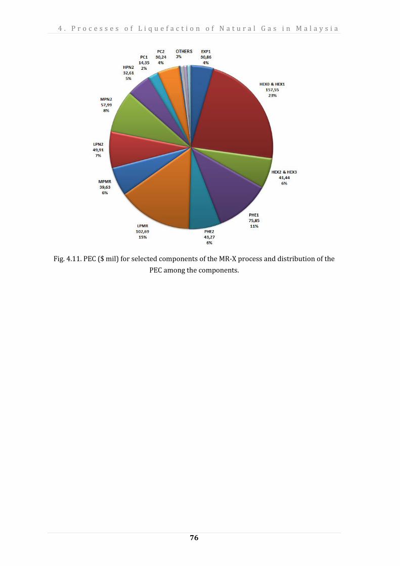
4 . P r o c e s s e s o f L i q u e f a c t i o n o f N a t u r a l G a s i n M a l a y s i a
76
Fig. 4.11. PEC ($ mil) for selected components of the MR-X process and distribution of the
PEC among the components.

4 . P r o c e s s e s o f L i q u e f a c t i o n o f N a t u r a l G a s i n M a l a y s i a
77
Table 4.3. Estimation of the fixed-capital investment.
2013 $
Direct costs
Onsite costs
Total purchased equipment cost (PEC) 700
PEC installation (45% of PEC) 315
Piping (35% of PEC) 245
Instrumentation and control (20 % of PEC) 140
Electrical equipment and materials (20% of PEC) 140
Total onsite costs 1540
Offsite costs 0
Total direct costs 1540
Indirect costs
Engineering and supervision (35% of PEC) 245
Construction costs (15% of DC) 231
Contingencies (10% of IC) 48
Total indirect costs 524
Fixed-capital investment 2064
The calculation of fixed-capital investment (including assumptions made) is given in Table
4.3. Since the location of the evaluated LNG plant is unknown, office costs were not taken
into consideration. Based on the estimated fixed-capital investment and the assumptions for
the economic, financial, operating, and market input variables, the total revenue
requirement is calculated on a year-by-year basis. Finally, the non-uniform annual monetary
values associated with the investment (carrying charges, CC), operating, maintenance
(OMC), and fuel costs (FC) of the system being analyzed) are levelized, that is they are
converted into an equivalent series of constant payments (annuities). The series of annual
costs associated with carrying charges (CCj) and expenses (FCj and OMCj) for the jth year of
plant operation are not uniform. The levelized carrying charges are calculated as
( ) CRFInvestmentCapitalTotalCCL ×= (4.16)
where the capital-recovery factor (CRF) is given by
( )( ) 11
1
−+
+=
neff
neffeff
i
iiCRF
(4.17)
Here, the ieff is the average annual effective discount rate (cost of money), and n
denotes the plant economic life expressed in years.
For the fuel, the constant escalation levelization factor (CELF) calculates

4 . P r o c e s s e s o f L i q u e f a c t i o n o f N a t u r a l G a s i n M a l a y s i a
78
( )( ) CRF
k
kkFCCELFFCFC
FC
nFCFC
L−
−=×=
1
100
(4.18)
with eff
FCFC
i
rk
++
=1
1 and rFC = const. The term rFC denotes the average annual nominal
escalation rate for fuel cost. The levelized annual operating and maintenance costs OMCL are
given by
( )( ) CRF
k
kkOMCCELFOMCOMC
FC
nFCFC
L−
−=×=
1
100
(4.19)
with eff
OMCOMC
i
rk
++
=1
1 and rOMC = const, where rOMC is the average annual nominal escalation
rate for the operating and maintenance costs. Finally, the levelized total revenue
requirement (TRR) is obtained from
TRR = CC + FC + OMC (4.20)

4 . P r o c e s s e s o f L i q u e f a c t i o n o f N a t u r a l G a s i n M a l a y s i a
79
Fig. 4.12. Levelized total revenue requirement for the MR-X process using different
assumptions for the economic analysis: OMC as a function of CC - between 1% and 10% and
cost of the electricity – between 0.05 and 0.20 $/kWh.

4 . P r o c e s s e s o f L i q u e f a c t i o n o f N a t u r a l G a s i n M a l a y s i a
80
The following assumptions have been made for the economic analysis:
• The operating and maintenance costs are a function of the CC and are varied
between 1% and 10%.
• The cost of electricity is assumed to vary between 0.05 and 0.20 $/kWh.
• The LNG plant operates with a 100% capacity during 7446 hours per year
(capacity factor = 85%).
• The average cost of money is ieff= 10%.
• The plant economic life is n=20 years.
• The average general inflation rate is rn=2.5%.
It is fully considered that the reported economic data cannot be accepted as absolute
correct because no detailed cost information is given in the open literature. However, the
relative economic characteristics are also very helpful for evaluating novel (and non-
proven) processes.
Fig. 4.13. Cost per unit of mass of the liquefaction process when different assumptions for
the economic analysis are used.
The results obtained from the economic analysis show that approximately 46% of the total
PEC are associated with multi-flow, low-temperature heat exchangers; % − with turbomachinery and only 3% with the remaining equipment. The preliminary estimation of
the fixed-capital investment of the novel MR-X LNG process is 2.064 $ bn or 0.265 (2013 $
bn/MTA). These values correlate well with the data reported in this section and the data
associated with the C3MR and AP-X process plants. The operation and maintenance costs
affect significantly the economic performance of the LNG plant. At low fuel cost (cost of

4 . P r o c e s s e s o f L i q u e f a c t i o n o f N a t u r a l G a s i n M a l a y s i a
81
electricity), the values of CC and OMC are dominant. However, with increasing fuel cost
(0.10 $/kWh) the fuel costs became comparable with the CC and OMC and even dominate.
The cost of the liquefaction process varies between 0.07 and 0.19 $/kgLNG (Fig. 4.13) using
different assumptions for the economic analysis. The results obtained from the economic
analysis show that the assumptions made play a significant role. These assumptions refer to
the cost of electricity and to OMC (% of CC), i.e. they depend on the country where the LNG
plant is located.

82
5. Conclusion and Future Works
In this thesis, several high energy-intensity LNG plants have been evaluated using energetic,
exergetic and economic analyses. A new LNG process concept has been designed, the MR-X
process, and has been analyzed to evaluate its thermodynamic and economic performances
and efficiency. All LNG processes possess particular characteristics where direct comparison
may not produce accurate perspectives. Nevertheless, in improving existing processes and
designing the new ones, scientists generally implement at least a general benchmark on
current technologies the world realistically has, and from where and how they can proceed
further.
Among important parameters to understand and analyze the LNG processes are
their principle of operations, through practical simulations and methodologies to analyze
them. While many ways are available for researchers to select in understanding and
bringing the technologies to the next level, practical solutions are significant especially to
the process owners and their stakeholders. The LNG circuits are complex enough, and in
analyzing them properly and practically without losing important characteristics are
delicate. Simulating the LNG process in Aspen was helpful, and many potentials for future
works are derived from such platform. However, like many other tool, the methodologies,
including energetic, exergetic, and economic analyses, have rooms for improvements. The
LNG processes itself, for example their multi-components compositions, compressor-power
arrangement, and heat exchangers’ duty are as well have various ways for further
advancement.
The newly introduced MR-X process combines the advantages and as much as
possible overcomes the limitations of the C3MR, AP-X and DMR processes. The MR-X system
coefficient of the performance and the exergetic efficiency are equal to 0.58 and 32%,
respectively. These relatively high values demonstrate that the novel process is efficient
from the thermodynamic viewpoint.
The preliminary estimation of the fixed-capital investment for the MR-X system
leads to 2.064 $ bn or 0.265 (2013 $ bn/MTA). The values reported for the AP-X plant are
slightly higher. This is an important point that should be clarified in the future, i.e. the effect
of the assumptions used for the economic analysis of an LNG plant needs to be studied.
Advanced exergy-based methods are recommended to be applied in the future, to obtain
more accurate and more specific information about the options for improving the
performance of the novel MR-X process from the economic and environmental viewpoints.

5 . C o n c l u s i o n a n d F u t u r e W o r k s
83
The AP-X process is the largest LNG power plant so far exists. The process is not only
complex due to its multi-component refrigeration in the MCHE, but it also uses the classical
pure propane refrigerant to precool a never-seen-in-history LNG capacity. The economics of
scale could be used for its justification, however the use of mixed-refrigerant as the
precooling agent is engaging, as per proven by the MR-X process. The AP-X system
coefficient of the performance and the exergetic efficiency are equal to 0.41 and 6%,
respectively. 24% of the total exergy destruction is associated with the multi-flow heat
exchanger HEX0 and HEX1. These are the MCHE which developers are strict on their data
confidentiality. The values may have better accuracies should more information about the
system and the system components publicly available, and advanced exergy is implemented,
where the interdependence between the components as well as the real potential for
improving the overall system will be discovered and discussed. The preliminary estimation
of the fixed-capital investment for the MR-X system leads to 5.8 $ bn or 0.95 (2013 $
bn/MTA).
Since all LNG processes are not only energy-intensive but also cost- and
environmental-impact-intensive, the design of the heat exchanger should be a central focus
of such LNG plants, especially the heat transfer characteristics. Despite the fact that the
investment cost of the heat exchanger is relatively high due to the large heat transfer surface
and to a complex and unique design, decreasing the inefficiencies within this component
and accepting higher investment cost will finally lead to a significant decrease in the overall
cost of the generated LNG.
In other perspective, for example the view of current global awareness and practical
applications in many governmental and societal levels to protect the earth against global
warming and ozone layer depletion, the selection and usage of refrigerants in the
liquefaction of natural gas should be considered essential. There are adverse effects
generated from the usage of the refrigerants, categorically could be in two perspectives: 1)
direct effect, and 2) indirect effects.
The direct effects are widely known for the past decades, as the development of non-
toxic and non-flammable refrigerants happening throughout the globe, and the application
of Montreal and Kyoto protocols at almost all countries and refrigerant manufacturers.
Notably while these developments and protocols are being actively referred to, the
flammable and toxic refrigerants may still exist because of research and military necessities.
Moreover, while direct effects are often clear for us to point out, the indirect effects of the
refrigerants are not so clear. LNG plants particularly in Malaysia have moved from steam-
based drivers towards gas-turbine drivers. The steam-based components, compared to the
current gas-turbine driven system, have more mechanical parts and, therefore, are less
efficient in electricity consumption as fuel. However, present gas-turbine drivers are still
dependent on fossil fuel-based starters.
In general, the indirect effects are due to the involvement of electricity or mechanical
components that needed to drive these refrigerants. The electrical and mechanical parts of

5 . C o n c l u s i o n a n d F u t u r e W o r k s
84
the LNG system need to be driven by fossil fuel that in turn indirectly contaminates earth's
environment. Subsequently, this contamination would cost LNG plant provider in monies
term where local government policies restricted the environment contamination. Indirectly
also, the reputation and future opportunities for these fossil-fuel-plant companies are in
risks.
The FLNG process is very near future work for LNG scientists. So far while there are
only Malaysian and Australian FLNG systems, the world is racing harder than before in this
new technology where different challenges are to be embraced. Deeper and stranded gas
reserves are becoming reachable than before as demand in higher quality of energy as well
as in environmental protection are increasing. As Malaysian LNG provider is the current
global pioneer on FLNG, studies on the sloshing effect of refrigerants and natural gas being
liquefied on ship, as well as all analyses done in this thesis and their proposals as future
works could be executed on this offshore process.
The analyzed MR-X process has shown the beneficial use of the mixed-refrigerant.
While not denying the use of Nitrogen as the sole refrigerant in the recently-launched AP-
NTM FLNG system, exergetic efficiency may come in handy in seeing these processes in terms
of exergetic efficiency performance and their exergy destructions. Furthermore,
exergoeconomics and exergoenvironmental analyses should be applied, that will provide
clearer reasonable and practical results on this latest LNG arena.

85
6. References
[1] HAMKA - Oxford Islamic Studies Online
http://www.oxfordislamicstudies.com/article/opr/t125/e795 (accessed April 27, 2015).
[2] Murphy T. Galactic-Scale Energy | Do the Math 2011. http://physics.ucsd.edu/do-the-
math/2011/07/galactic-scale-energy/ (accessed March 4, 2015).
[3] Exponential Growth and Energy Consumption - World Population Balance - sustainable
world US population. http://www.worldpopulationbalance.org/growth_and_energy
(accessed March 4, 2015).
[4] Kidnay AJ, Parrish WR. Fundamentals of Natural Gas Processing. Taylor and Francis
Group, LLC; 2006.
[5] Zaïm A. Dynamic Optimization of an LNG Plant: Case Study: GL2Z LNG Plant in Arzew,
Algeria. Shaker, 2002.
[6] BP. BP Energy Outlook 2035. 2015.
[7] McKay J. For The Record. LNG Journal 2015.
[8] Energy Information Administration. Natural Gas 1998 Issues and Trends. US Department
of Energy 1999;0560.
[9] Foss MM. Introduction To LNG - An overview on liquefied natural gas (LNG), its
properties, organization of the LNG industry and safety considerations. Austin, Texas:
Center for Energy Economics; 2007.
[10] The International Group of Liquefied Natural Gas Importers (GIIGNL). The LNG Process
Chain. Levallois: 2009.
[11] DOE/EIA-0637. The Global Liquefied Natural Gas Market: Status & Outlook. Vol. 0637.
2003.
[12] Al-Saadoon FT, Nsa AU. Economics of LNG Projects. Proceedings of SPE Production and
Operations Symposium 2009. doi:10.2118/120745-MS.
[13] Harjono P. Testimony of President - Director of Pertamina before the Federal Power
Commission. 1977.
[14] Project Structure, Cost, and Financing. The Future of Liquefied Natural Gas Imports, p.
68–106.
[15] International Gas Union. World LNG Report - 2014 Edition. 2014.
[16] Yang CC, Kaplan A, Huang Z. Cost-effective design reduces C2 and C2 at LNG receiving
terminals. Oil & Gas Journal 2003.
[17] Petronas MLNG. http://www.mlng.com.my (accessed May 15, 2015).
[18] The Petroleum Economist Ltd. World LNG Map. 1998.
[19] IEA, OECD. NATURAL GAS MARKET REVIEW - Security in a globalising market to 2015.
International Energy Agency 2007.

6 . R e f e r e n c e s
86
[20] Woodside Wants Three FLNG Facilities at Browse| Offshore Energy Today.
http://www.offshoreenergytoday.com/woodside-wants-three-flng-facilities-at-browse/
(accessed September 25, 2014).
[21] Air Products’ LNG Expertise Selected for Second Malaysia PETRONAS FLNG Project -
Yahoo Finance. http://finance.yahoo.com/news/air-products-lng-expertise-selected-
065500120.html (accessed September 25, 2014).
[22] Morosuk T., Omar M.N.B, Tsatsaronis G., Naw R. Advanced Exergetic Analysis of a
Refrigeration System for Liquefaction of Natural Gas. Proceedings of the 23-rd
International Conference on Efficiency, Cost, Optimization Simulation and Environmental
Impact of Energy Systems (ECOS2010), Lausanne, Switzerland, 2010.
[23] Morosuk T., Hiemann A., Omar M.N.B., Tsatsaronis G. Exergy-Based Methods Applied to
the Chain “NATURAL GAS – LNG – NATURAL GAS” − Liquefaction Using a Single Mixed-
Refrigerant Process. 3rd International Exergy, Life Cycle Assessment, and Sustainability
Workshop & Symposium (ELCAS3) 07 -09 July, 2013, Nisyros, Greece, 2013.
[24] Morosuk T., Tesch S., Hiemann A., Tsatsaronis G., Omar M.N.B. Evaluation of the PRICO
liquefaction process using exergy-based methods. Journal of Natural Gas Science and
Engineering 2015:1–9. doi:10.1016/j.jngse.2015.02.007.
[25] Black&Veatch. www.bv.com.
[26] Roberts MJ, Liu Y, Bronfenbrenner JC, Solomon J, James C. Technology selection. USA,
2004.
[27] Remeljej C, Hoadley A. An exergy analysis of small-scale liquefied natural gas (LNG)
liquefaction processes. Energy 2006;31:2005–19. doi:10.1016/j.energy.2005.09.005.
[28] Jensen JB, Skogestad S. Single-cycle mixed-fluid LNG process Part I: Optimal design. 1st
Annual Gas Processing Symposium, Doha, Qatar, 2009.
[29] Aspelund A, Gundersen T, Myklebust J, Nowak MP, Tomasgard A. An optimization-
simulation model for a simple LNG process. Computers & Chemical Engineering
2010;34:1606–17. doi:10.1016/j.compchemeng.2009.10.018.
[30] Shirazi MMH, Mowla D. Energy optimization for liquefaction process of natural gas in
peak shaving plant. Energy 2010;35:2878–85. doi:10.1016/j.energy.2010.03.018.
[31] Lee GC. Optimal design and anaylysis of refrigeration systems for low temperature
processes. The University of Manchester, 2001.
[32] Hiemann A. Energy and Exergy Analysis of a Single Mixed Refrigerant Process for the
Liquefaction of Natural Gas. 2011.
[33] Marmolejo-Correa D, Gundersen T. A comparison of exergy efficiency definitions with
focus on low temperature processes. Energy 2012;44:477–89.
doi:10.1016/j.energy.2012.06.001.
[34] Xu X, Liu J, Jiang C, Cao L. The correlation between mixed refrigerant composition and
ambient conditions in the PRICO LNG process. Applied Energy 2013;102:1127–36.
doi:10.1016/j.apenergy.2012.06.031.
[35] Morin A, Wahl PE, Mølnvik M. Using evolutionary search to optimise the energy
consumption for natural gas liquefaction. Che E g Res Des ; : 4 − 44 .
[36] Wahl PE, Løvseth SW, Mølnvik MJ. Optimization of a simple LNG process using sequential
quadratic programming. Computers & Chemical Engineering 2013;56:27–36.
doi:10.1016/j.compchemeng.2013.05.001.
[37] Castillo L, Dorao C A. Consensual decision-making model based on game theory for LNG

6 . R e f e r e n c e s
87
processes. Energy Conversion and Management 2012;64:387–96.
doi:10.1016/j.enconman.2012.06.014.
[38] Khan MS, Lee S, Lee M. Optimization of single mixed refrigerant natural gas liquefaction
plant with nonlinear programming. Asia-Pacific Journal of Chemical Engineering
2012;7:258–61. doi:10.1002/apj.642.
[39] Khan MS, Lee S, Rangaiah GP, Lee M. Knowledge based decision making method for the
selection of mixed refrigerant systems for energy efficient LNG processes. Applied Energy
2013;111:1018–31. doi:10.1016/j.apenergy.2013.06.010.
[40] Heldt S. Near-optimal operation of LNG Liquefaction processes by means of regulation.
2011.
[41] Barclay MA, Yang CC. Offshore LNG: The Perfect Starting Point for the 2-Phase Expander?
Offshore Technology Conference, Texas, 1-4 May, vol. OTC 18012, 2006.
[42] Barclay M, Denton N. Selecting offshore LNG processes. LNG Journal 2005:34–6.
[43] Roberts MJ, Bronfenbrenner JC, Liu Y-N, Petrowski JM. Large Capacity Single Train AP-
XTM Hybrid LNG Process. GASTECH2002, Qatar, 2002.
[44] Kasmuni AA, Ann GN, Regterschot J. THE MALAYSIA LNG COMPLEX — SUSTAINABLE
GROWTH. Thirteenth International Conference on Liquefied Natural Gas, Institute of Gas
Technology; 2001, p. 3.
[45] Lim W, Choi K, Moon I. Current Status and Perspectives of Liquefied Natural Gas (LNG)
Plant Design. Industrial & Engineering Chemistry Research 2013:3065–88.
doi:dx.doi.org/10.1021/ie302877g.
[46] Bosma P, Nagelvoort RK. Liquefaction Technology; Developments through History.
Proceedings of the 1st Annual Gas Processing Symposium, 2009.
[47] Maritime Content Ltd. LNG16 cloud cleared to reveal Sunrise FLNG project decision
commercial success Publisher Editor. LNG Journal 2010.
[48] Ismail NH, Grootjans H. THE MLNG TIGA PROJECT. LNG 12, Perth, Australia. May 4-7,
1998.
[49] Ismail NH, Ariffin MS, Omori H, Konishi H, Ray SA, Durr CA. Application of Dynamic
Simulation for Design and Commissioning of LNG Plants (Experience in MLNG Tiga
Project). LNG 14, Doha, Qatar, March 2004.
[50] Roberts MJ, Agrawal R. Hybrid cycle for the production of liquefied natural gas. US Patent
6308531, 2001.
[51] Omar M.N.B., Morosuk T, Tsatsaronis G. Exergy Analyses Applied to an AP-X Process for
the Liquefaction Of Natural Gas. Proceedings of the ASME 2012 International Mechanical
Engineering Congress & Exposition IMECE2012, Houston, Texas, 2012.
[52] Gas: Fueling the future of energy – BorneoPost Online
http://www.theborneopost.com/2013/10/20/gas-fueling-the-future-of-energy/
(accessed September 16, 2014).
[53] Bukowski JD, Liu Y-N, Pillarella M, Boccella SJ, Kennington WA. NATURAL GAS
LIQUEFACTION TECHNOLOGY FOR FLOATING LNG FACILITIES. LNG 17 Conference:
Floating LNG Facilities, Houston, Texas, 2013.
[54] Howe B, Skinner G, Maunder T. UK’s Gasconsult ZR-LNG liquefaction technology aims to
make impact with new mid-scale solution. LNG Journal 2013:28–32.
[55] International Gas Union (IGU). ACCESS TO ENERGY - Gas delivers sustainable economic
development.

6 . R e f e r e n c e s
88
[56] Omar M.N.B., Morosuk T., Tsatsaronis G. Thermodynamic And Economic Evaluation Of A
Novel Mixed-Refrigerant Process For The Liquefaction Of Natural Gas. Proceedings of the
ASME2014 International Mechanical Engineering Congress & Exposition (IMECE2014),
Montreal, Canada, 2014.
[57] Malaysia to be LNG import-free nation by 2016, says Petronas senior official | Malay Mail
Online. http://www.themalaymailonline.com/money/article/msia-to-be-lng-import-free-
nation-by-2016-says-petronas-senior-official (accessed March 10, 2015).
[58] Philip R. Weems (King & Spalding LLP), Harry W. Sullivan J (ConocoPhillips). LNG at 50 -
History and Projected Future for Liquefied Natural Gas Exports in an Unconventional Era.
RMMLF 60th Annual Institute 2014.
[59] PETROLEUM ECONOMIST. WGC News 2012.
[60] Barclay M, Shukri T, L. N. G. Consultants. Enhanced single mixed refrigerant process for
stranded gas liquefaction. 79th Annual Gas Processors Association Convention, Atlanta,
2000.
[61] Tsatsaronis G, Cziesla F. Exergy Analysis of a Simple Process. Encyclopedia of Life Support
Systems (EOLSS), UNESCO, Eolss Publishers, 2004.
[62] Bejan A, Tsatsaronis G, Moran MJ. Thermal Design and Optimization. John Wiley & Sons,
1996.
[63] Ahrends J. Reference States. Energy - The International Journal 1980:667–77.
[64] Szargut J, Morris DR, Steward FR. Exergy Analysis of Thermal, Chemical and Metallurgical
Processes. New York, Hemisphere Publishing Corporation, 1988.
[65] Morosuk T, Tsatsaronis G. A New Approach to the Exergy Analysis of Absorption
Refrigeration Machines. Energy – The International Journal 2008;33:890–907.
[66] The software is a proprietary product of AspenTech. Aspen Plus 2012;V7.3.2.
[67] Aspen Technology Inc. Aspen Physical Property System - Physical Property Methods V7.2
2010.
[68] Aspen Technology Inc. Getting Started Building Model.
[69] The software is part of Microsoft Office 365. Microsoft® Excel 2013.
[70] Seider WD, Seader JD, Lewi DR. Product a d Process Desig Pri ciples : Sy thesis, Analysis, and Evaluation. Second Edi. Wiley, 2003.
[71] Van Driel A, Nagelvoort RK, Pek BJJ, de Jong ECJN. Large Capacity LNG Plant
Development. LNG-14, Qatar: Shell Global Solutions International B.V., 2004.
[72] Neeraas BO, Fredheim AO, Aunan B. Experimental shell-side heat transfer and pressure
drop in gas flow for spiral-wound LNG heat exchanger. International Journal of Heat and
Mass Transfer 2004;47:353–61. doi:10.1016/S0017-9310(03)00400-9.
[73] Hill RWS. Exergy Analysis Applied to a C3MR Process for the Liquefaction of Natural Gas.
Technical University Berlin, 2012.
[74] Venkatarathnam G. CRYOGENIC MIXED REFRIGERANT PROCESSES International
cryogenics monograph series. Springer Science + Business Media. LLC; 2008.
[75] Pillarella M, Liu Y-N, Petrowski J, Bower R. The C3MR Liquefaction Cycle: Versatility For A
Fast Growing, Ever Changing LNG Industry. Presentation at the 15th International
Conference on LNG, Barcelona, Spain, April 2007, 2007.
[76] Rigby J, Ramsay G, Featherston WA, Potter A, Wood A, Brooks A. UBS Investment
Research Global Oil & Gas 2008.

6 . R e f e r e n c e s
89
[77] Castillo L, Dorao CA. On the conceptual design of pre-cooling stage of LNG plants using
propane or an ethane/propane mixture. Energy Conversion and Management
2013;65:140–6. doi:10.1016/j.enconman.2012.07.015.
[78] Rivera V, Aduku A, Harris O. Evaluation of LNG Technologies. University of Oklahoma,
2008.
[79] Shukri T. LNG technology selection. 2004.
[80] Laurents G. LNG Processing and On Stream Analysis. 2007.
[81] Madhavan S. LNG Technology. Dehra Dun, 2010.
[82] Bass N, Al-Aidaroos S, Downey B, Ziegler J. Offshore LNG Production 2009.
[83] Topal E. Exergoeconomic analysis of a plant for the liquefaction of natural gas. Master
thesis. Technische Universität Berlin, 2013.
[84] Roberts MJ, Petrowski JM, Liu Y-N. Reducing LNG capital cost in today’s competitive
environment 2007:1–12.
[85] Bukowski J, Liu YN, Boccella SJ, Kowalski L. Innovations in natural gas liquefaction
technology. International Gas Union Research Conference 2011, 2011.
[86] Cengel YA, Boles MA. Thermodynamics: An Engineering Approach. 2nd ed. McGraw-Hill
Inc., 1994.
[87] DiNapoli R., Yost C. Benchmarking study compares LNG plant costs. Oil & Gas Journal
2003;14.
[88] A liquid market | The Economist. http://www.economist.com/node/21558456 (accessed
May 19, 2015).
[89] Heath T, Tidy M. How to penetrate the global lng market. 2005.
[90] Jensen JT. The Outlook for Global Trade in Liquefied Natural Gas Projections To the Year
2020. 2007.
[91] Hashimoto H. Evolving Roles of LNG and Asian Economies in the Global Natural Gas
Markets. Pacific Energy Summit, Jakarta, 2011.
[92] Bronfenbrenner JC, Pillarella M, Solomon J. Selecting A Suitable Process.
LNGINDUSTRYCOM 2009.
[93] Venkatarathnam G. Chapter 6. Natural gas liquefaction processes, 2008.
doi:10.1007/978-0-387-78514-1_6.
[94] Omar M.N.B., Morosuk T, Tsatsaronis G. A Novel Mixed-Refrigerant Process for the
Liquefaction of Natural Gas. Proceedings of ECOS 2014 - The 27th International
Conference on Efficiency, Cost, Optimization, Simulation and Environmental Impact of
Energy Systems on June 15-19, Turku, Finland, 2014.
[95] Dolatshahi A, Amidpour M. Exergy Analysis of Propane Pre-cooled Mixed Refrigerant
Process Used in LNG Plants. Proceedings of the 23-rd International Conference on
Efficiency, Cost, Optimization Simulation and Environmental Impact of Energy Systems,
Lausanne, Swiss, 2010, p. 1872–7.
[96] Alabdulkarem A, Mortazavi A, Hwang Y, Radermacher R, Rogers P. Optimization of
propane pre-cooled mixed refrigerant LNG plant. Applied Thermal Engineering
2011;31:1091–8. doi:10.1016/j.applthermaleng.2010.12.003.
[97] Morosuk T, Tsatsaronis G. A new approach to the exergy analysis of absorption
refrigeration machines. Energy 2008;33:890–907. doi:10.1016/j.energy.2007.09.012.
[98] Greaker M, Lund Sagen E. Explaining experience curves for new energy technologies: A

6 . R e f e r e n c e s
90
case study of liquefied natural gas. Energy Economics 2008;30:2899–911.
doi:10.1016/j.eneco.2008.03.011.
[99] Lazzaretto A, Tsatsaronis G. SPECO: A systematic and general methodology for calculating
efficiencies and costs in thermal systems. Energy 2006;31:1257–89.
doi:10.1016/j.energy.2005.03.011.
[100] Seider WD, Seader JD, Lewin DR. Product & Process Design Principles - Synthesis, Analysis
& Evaluation. Chemistry 2003:728.
[101] Kakac S, Liu H, Pramuanjaroenkij A. Heat exchangers: selection, rating, and thermal
design. CRC press, 2012.
[102] IGU World LNG Report - 2013 Edition. 2013.
[103] Mckeever J, Pillarella M, Bower R. LNG Industry - An ever evolving technology. Air
Products and Chemicals 2008.
[104] Department of Mechanical Engineering Technical University of Denmark. Cool Pack
Version 1.46 2000.
[105] Air Products’ LNG Expertise Selected for PETRONAS FLNG Project in Malaysia.
http://www.airproducts.com/company/news-center/2012/07/0718-air-products-lng-
expertise-selected-for-petronas-flng-project-in-
malaysia.aspx?utm_source=&utm_medium=NR&utm_campaign=fy1
3-News-Release (accessed June 30, 2014).
[106] Verein Deutscher Ingenieure, Gesellschaft Verfahrenstechnik und
Chemieingenieurwesen. VDI-Wärmeatlas: Berechnungsblätter für den Wärmeübergang.
Springer, 2002.
[107] Emmet G. International construction cost survey 2012. Turner & Townsend Plc 2012:1–
42.
[108] Tenaga Nasional Berhad. Pricing & Tariff 2011. http://www.tnb.com.my/business/for-
industrial/pricing-tariff.html#industrial (accessed April 12, 2013).
[109] Suprapto YP. Chapter 30 - LNG Technology - Processes. LNG & the World of Energy,
Indonesia: PT Badak NGL, 2007.
91
Appendix A. Research
Contributions
1. Morosuk T, Tesch S, Hiemann a., Tsatsaronis G, Bin Omar N. 2015.
“Evaluation of the PRICO liquefaction process using exergy-based methods.”
Journal of Natural Gas Science and Engineering.
2. Bin Omar MN, Morosuk T, Tsatsaronis G. 2014.
“Thermodynamic And Economic Evaluation Of A Novel Mixed-Refrigerant Process
For The Liquefaction Of Natural Gas.”
Proceedings of the ASME2014 International Mechanical Engineering Congress &
Exposition (IMECE2014), Montreal, Canada.
3. Bin Omar N, Morosuk T, Tsatsaronis G. 2014.
“A Novel Mixed-Refrigerant Process for the Liquefaction of Natural Gas.”
Proceedings of ECOS 2014 - The 27th International Conference on Efficiency, Cost,
Optimization, Simulation and Environmental Impact of Energy Systems on June 15-
19, Turku, Finland.
4. T. Morosuk, A. Hiemann, N. Bin Omar, Tsatsaronis G. 2013.
“Exergy-Based Methods Applied To The Chain “Natural Gas – LNG – Natural Gas” − Liquefaction Using A Single Mixed-Refrigerant Process.”
3rd International Exergy, Life Cycle Assessment, and Sustainability Workshop &
Symposium (ELCAS3) 07-09 July, 2013, NISYROS – GREECE.
5. Omar MN Bin, Morosuk T, Tsatsaronis G. 2012.
“Exergy Analyses Applied to an AP-X Process for the Liquefaction Of Natural Gas.”
Proceedings of the ASME 2012 International Mechanical Engineering Congress &
Exposition IMECE2012, Houston, Texas.
6. Morosuk T, Nazri M, Omar B, Tsatsaronis G, Naw R. 2010.
“Advanced Exergetic Analysis of a Refrigeration System for Liquefaction of Natural
Gas.”
Proceedings of the 23-rd International Conference on Efficiency, Cost, Optimization
Simulation and Environmental Impact of Energy Systems (ECOS2010), Lausanne,
Switzerland.

92
Appendix B. Energy and Exergy
Analyses – Data, Flow and
Results
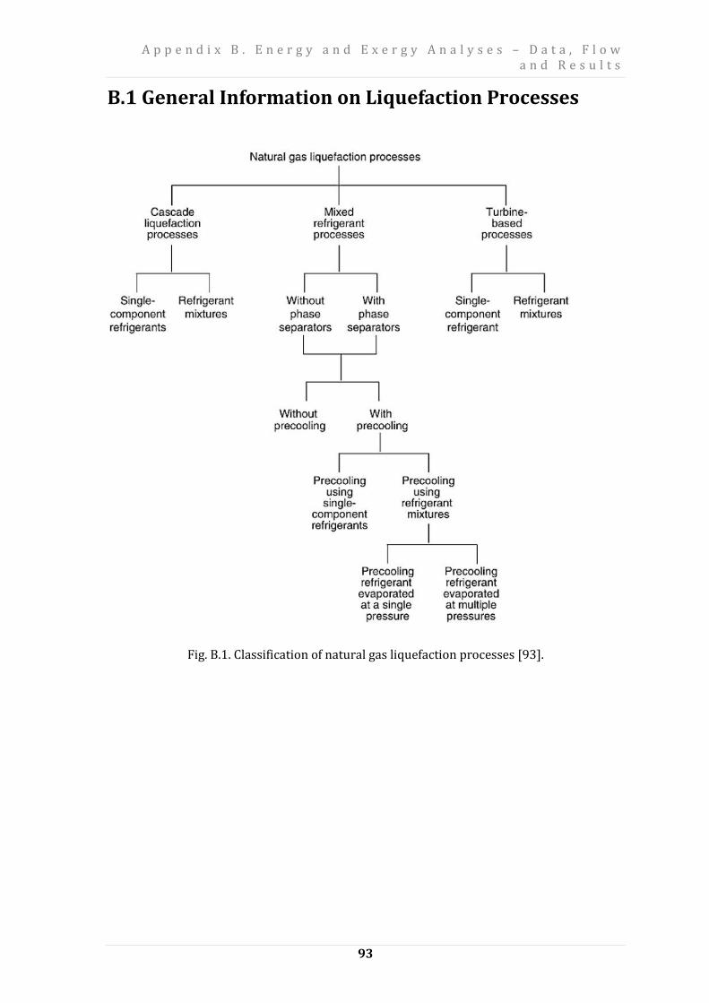
A p p e n d i x B . E n e r g y a n d E x e r g y A n a l y s e s – D a t a , F l o w a n d R e s u l t s
93
B.1 General Information on Liquefaction Processes
Fig. B.1. Classification of natural gas liquefaction processes [93].

A p p e n d i x B . E n e r g y a n d E x e r g y A n a l y s e s – D a t a , F l o w a n d R e s u l t s
94
Table B.1. Malaysian LNG Plants.
Bintulu MLNG
Satu
Bintulu MLNG
Dua
Bintulu MLNG
Tiga
PETRONAS
Floating LNG
Project 1
(PFLNG 1)
PETRONAS
Floating LNG
Project 2
(PFLNG 2)
Start-up 1983 1995 2003 Late 2015 2018
Operator MLNG Satu MLNG Dua MLNG Tiga PFLNG 1 PFLNG 2
Shareholders
PETRONAS
(60%), Shell
(17.5%),
Mitsubishi
(17.5%),
Sarawak state
government
(5%)
PETRONAS
(60%), Shell
(15%),
Mitsubishi
(15%),
Sarawak state
government
(10%)
PETRONAS
(60%), Shell
(10%), Nippon
Oil (10%),
Occidental
LNG Malaysia
(10%),
Sarawak state
government
(10%)
(TBC) (TBC)
Capacity
(MMTPA) 8.1 7.8 6.8 1.2 1.5
No. of trains 3 3 2 1 1
LNG process
type
Air Products’
C3MR
Air Products’
C3MR
Air Products’
C3MR
Air Products’
AP-NTM
Air Products’
AP-NTM
Gas fields Central
Luconia Basin
Central
Luconia Basin Jintan
Kanowit
(offshore
Sarawak)
Rotan
(offshore
Sabah)

A p p e n d i x B . E n e r g y a n d E x e r g y A n a l y s e s – D a t a , F l o w a n d R e s u l t s
95
Table B.2. Liquefaction Plants with specific LNG Technology, sorted by year of project start [102].
Country Project Name Start Year
Nameplate Capacity (mmtpa)
Owners Liquefaction Technology
US Kenai LNG* 1969 1.5 ConocoPhillips ConocoPhillips
Optimized Cascade®
Algeria Skikda - GL1K (T1-4) 1972 1 Sonatrach Teal (T1-3), PRICO (T4)
Brunei Brunei LNGT1-5 1972 7.2 Government of Brunei, Shell, Mitsubishi APC C3MR
Indonesia Bontang LNG T1-2 1977 5.4 Pertamina APC C3MR
United Arab Emirates
ADGAS LNGT1-2 1977 2.6 ADNOC, Mitsui, BP, TOTAL APC C3MR
Algeria Arzew- GL1Z (T1-6) 1978 6.6 Sonatrach APC C3MR
Indonesia Arun LNG T1 1978 1.65 Pertamina APC C3MR
Algeria Arzew-GL2Z (T1-6) 1981 8.2 Sonatrach APC C3MR
Algeria Skikda - GL2K (T5-6) 1981 2.2 Sonatrach PRICO
Indonesia Bontang LNG T3-4 1983 5.4 Pertamina APC C3MR
Malaysia MLNG Satu (T1-3) 1983 8.1 PETRONAS, Mitsubishi, Sarawak State government APC C3MR
Indonesia Arun LNG T6 1986 2.5 Pertamina APC C3MR
Australia North West Shelf T1 1989 2.5 BHP Billiton, BP, Chevron, Shell, Woodside, Mitsubishi,
Mitsui APC C3MR
Australia North West Shelf T2 1989 2.5 BHP Billiton, BP, Chevron, Shell, Woodside, Mitsubishi,
Mitsui APC C3MR
Indonesia Bontang LNG T5 1989 2.9 Pertamina APC C3MR
Australia North West Shelf T3 1992 2.5 BHP Billiton, BP, Chevron, Shell, Woodside, Mitsubishi,
Mitsui APC C3MR
Indonesia Bontang LNG T6 1994 2.9 Pertamina APC C3MR
United Arab Emirates
ADGAS LNG T3 1994 3.2 ADNOC, Mitsui, BP, TOTAL APC C3MR
Malaysia MLNG Dua (T1-3) 1995 7.8 PETRONAS, Shell, Mitsubishi, Sarawak State government APC C3MR
Qatar Qatargas I (T1) 1997 3.2 Qatar Petroleum, ExxonMobil, TOTAL, Marubeni, Mitsui APC C3MR
Qatar Qatargas I (T2) 1997 3.2 Qatar Petroleum, ExxonMobil, TOTAL, Marubeni, Mitsui APC C3MR
Indonesia Bontang LNG T7 1998 2.7 Pertamina APC C3MR
Qatar Qatargas I (T3) 1998 3.1 Qatar Petroleum, ExxonMobil, TOTAL, Mitsui, Marubeni APC C3MR

A p p e n d i x B . E n e r g y a n d E x e r g y A n a l y s e s – D a t a , F l o w a n d R e s u l t s
96
Indonesia Bontang LNG T8 1999 3 Pertamina APC C3MR
Nigeria NLNGT1 1999 3.3 NNPC, Shell, TOTAL, Eni APC C3MR
Qatar RasGas I (T1) 1999 3.3 Qatar Petroleum, ExxonMobil, KOGAS, Itochu, LNG Japan APC C3MR
Trinidad ALNG T1 1999 3.3 BP, BG, Repsol, CIC, NGC Trinidad ConocoPhillips
Optimized Cascade®
Nigeria NLNG T2 2000 3.3 NNPC, Shell, TOTAL, Eni APC C3MR
Oman Oman LNG T1 2000 3.55 Petroleum Development Oman (PDO), Shell, TOTAL,
Korea LNG, Partex, Mitsubishi, Mitsui, Itochu APC C3MR
Oman Oman LNG T2 2000 3.55 Petroleum Development Oman (PDO), Shell, TOTAL,
Korea LNG, Partex, Mitsubishi, Mitsui, Itochu APC C3MR
Qatar RasGas I (T2) 2000 3.3 Qatar Petroleum, ExxonMobil, KOGAS, Itochu, LNG Japan APC C3MR
Nigeria NLNGT3 2002 3 NNPC, Shell, TOTAL, Eni APC C3MR
Trinidad ALNG T2 2002 3.5 BP, BG, Repsol ConocoPhillips
Optimized Cascade®
Malaysia MLNG Tiga (T1-2) 2003 6.8 PETRONAS, Shell, Nippon, Sarawak State government,
Mitsubishi APC C3MR
Trinidad ALNG T3 2003 3.5 BP, BG, Shell ConocoPhillips
Optimized Cascade®
Australia North West Shelf T4 2004 4.4 BHP Billiton, BP, Chevron, Shell, Woodside, Mitsubishi,
Mitsui APC C3MR
Qatar RasGas II (T1) 2004 4.7 Qatar Petroleum, ExxonMobil APC C3MRI Split MR™
Egypt ELNG T1 2005 3.6 BG, PETRONAS, EGAS, EGPC, GDF SUEZ ConocoPhillips
Optimized Cascade®
Egypt ELNG T2 2005 3.6 BG, PETRONAS, EGAS, EGPC ConocoPhillips
Optimized Cascade®
Egypt SEGAS T1 2005 5 Gas Natural Fenosa, Eni, EGPC, EGAS APC C3MRI Split MR™
Qatar RasGas II (T2) 2005 4.7 Qatar Petroleum, ExxonMobil APC C3MRI Split MR™
Australia Darwin LNG T1 2006 3.6 ConocoPhillips, Santos, INPEX, Eni, TEPCO, Tokyo Gas ConocoPhillips
Optimized Cascade®
Nigeria NLNG T4 2006 4.1 NNPC, Shell, TOTAL, Eni APC C3MR
Nigeria NLNG T5 2006 4.1 NNPC, Shell, TOTAL, Eni APC C3MR
Oman Qalhat LNG 2006 3.7 Omani Govt, Petroleum Development Oman (PDO), Shell,
Mitsubishi, Gas Natural Fenosa, Eni, Itochu, Osaka Gas, TOTAL, Korea LNG, Mitsui, Partex
APC C3MR
Trinidad ALNG T4 2006 5.2 BP, BG, Repsol, NGC Trinidad ConocoPhillips
Optimized Cascade®

A p p e n d i x B . E n e r g y a n d E x e r g y A n a l y s e s – D a t a , F l o w a n d R e s u l t s
97
Equatorial Guinea
EG LNGT1 2007 3.7 Marathon, Sonagas, Mitsui, Marubeni ConocoPhillips
Optimized Cascade®
Norway Snohvit LNG T1 2007 4.2 Statoil, Petoro, TOTAL, GDF SUEZ, RWE Linde MFC
Qatar RasGas II (T3) 2007 4.7 Qatar Petroleum, ExxonMobil APC C3MRI Split MR™
Australia North West Shelf T5 2008 4.4 BHP Billiton, BP, Chevron, Shell, Woodside, Mitsubishi,
Mitsui APC C3MR
Nigeria NLNG T6 2008 4.1 NNPC, Shell, TOTAL, Eni APC C3MR
Indonesia Tangguh LNG T1 2009 3.8 BP, CNOOC, Mitsubishi, INPEX, JOGMEC, JX Nippon Oil & Energy, LNG Japan, Talisman Energy, Kanematsu, Mitsui
APC C3MRI Split MR™
Indonesia Tangguh LNG T2 2009 3.8 BP, CNOOC, Mitsubishi, INPEX, JOGMEC, JX Nippon Oil & Energy, LNG Japan, Talisman Energy, Kanematsu, Mitsui
APC C3MRI Split MR™
Qatar Qatargas II (T1) 2009 7.8 Qatar Petroleum, ExxonMobil APC AP-X
Qatar Qatargas II (T2) 2009 7.8 Qatar Petroleum, ExxonMobil, TOTAL APC AP-X
Qatar RasGas III (T1) 2009 7.8 Qatar Petroleum, ExxonMobil APC AP-X
Russia Sakhalin 2 (T1) 2009 4.8 Gazprom, Shell, Mitsui, Mitsubishi Shell DMR
Russia Sakhalin 2 (T2) 2009 4.8 Gazprom, Shell, Mitsui, Mitsubishi Shell DMR
Yemen Yemen LNG T1 2009 3.35 TOTAL, Hunt Oil, Yemen Gas Co., SK Corp, KOGAS, GASSP,
Hyundai APC C3MRI Split MR™
Malaysia MLNG Dua Debottleneck 2010 1.2 PETRONAS, Shell, Mitsubishi, Sarawak State government APC C3MR
Norway Skangass LNG 2010 0.3 Skangass Linde LIMUM
Peru Peru LNG 2010 4.45 Hunt Oil, Repsol, SK Corp, Marubeni APC C3MRI Split MR™
Qatar Qatargas III 2010 7.8 Qatar Petroleum, ConocoPhillips, Mitsui APC AP-X
Qatar RasGas III (T2) 2010 7.8 Qatar Petroleum, ExxonMobil APC AP-X
Yemen Yemen LNG T2 2010 3.35 TOTAL, Hunt Oil, Yemen Gas Co., SK Corp, KOGAS, GASSP,
Hyundai APC C3MRI Split MR™
Qatar Qatargas IV 2011 7.8 Qatar Petroleum, Shell APC AP-X
Australia Pluto LNG T1 2012 4.3 Woodside, Kansai Electric, Tokyo Gas Shell propane precooled mixed refrigerant design

A p p e n d i x B . E n e r g y a n d E x e r g y A n a l y s e s – D a t a , F l o w a n d R e s u l t s
98
Fig. B.2. A typical coil-wound MCHE for a C3MR process-based LNG plant [103].
The picture on the LEFT side shows the coiling of the cooling tube and eventually will be
placed inside a bundled-shell shown in the RIGHT side. Apart from liquefaction purpose, the
shell directly serves as secondary protection in case of tube leakages thus adding more
value towards the selection of MCHE in LNG production.

A p p e n d i x B . E n e r g y a n d E x e r g y A n a l y s e s – D a t a , F l o w a n d R e s u l t s
99
B.2 System testing using PRICO® process [23,24,32]
Fig. B.3. Flow diagram of PRICO process: CM1 - Compressor 1; COL - Cooler; CM2 -
Compressor 2; CD - Condenser; HE - Heat exchanger; TV - Throttling Valve [24].
Table B.3. Composition and concentration of natural gas and refrigerants.
Component Formula Refrigerant [34] (% mol)
Natural gas [97] (% mol)
Methane CH4 0.30 0.88
Ethane C2H6 0.30 0.08
Propane C3H8 − 0.02
Butane C4H10 0.25 −
Nitrogen N2 0.15 0.02

A p p e n d i x B . E n e r g y a n d E x e r g y A n a l y s e s – D a t a , F l o w a n d R e s u l t s
100
Table B.4. Thermodynamic data for material streams at real operating conditions S
tre
am
Ma
teri
al
stre
am
m
(kg/s)
T
(ºC)
p
(bar)
x
(kg/kg)
h
(kJ/kg)
s
(kJ/kg K)
TE
(kW)
ME
(kW)
PHE
(kW)
1
Re
frig
era
nt
475
15 3 − -2443 -5.15 0.14 9.61 9.75
2 71 8 − -2345 -5.09 2.84 25.36 28.20
3 30 8 − -2320 -5.32 0.03 25.36 25.39
4 91 22 − -2313 -5.25 5.86 60.50 66.36
5 30 22 0.84 -2510 -5.87 0.08 61.36 61.44
6 -159 19 0 -3160 -9.22 94.29 133.25 227.53
7 -162 6 0.07 -3159 -9.19 108.33 114.07 222.39
8
Na
tura
l g
as
38 67 − -4162 -6.77 0.03 24.91 24.94
9 50 -159 64 0 -4999 -11.12 16.49 31.48 47.97
10 -163 1 0.05 -4999 -10.98 46.08 0.18 46.26
11 3 -163 1 1 -3403 -4.85 0.51 0.18 0.69
12 47 -163 1 0 -5088 -11.32 45.58 0.18 45.76
Table B.5. Reference values for the exergetic analysis (state 0) for material streams.
Stream Material stream
T
(ºC)
p
(bar)
h
(kJ/kg)
s
(kJ/kg K)
1 - 7 Refrigerant 25 1.013
-2426 -4.81
8-10 Natural gas -4141 -5.03

A p p e n d i x B . E n e r g y a n d E x e r g y A n a l y s e s – D a t a , F l o w a n d R e s u l t s
101
Table B.6. Detailed thermodynamic data of each chemical component in the streams within
mixed refrigerant.
Stream 1 2 3 4 5 6 7 8 9 10 11 12
Vapor Mass Fraction (kg/kg)
Methane 0.148 0.148 0.148 0.148 0.144 − 0.002 0.786 − 0.035 0.661 −
Ethane 0.277 0.277 0.277 0.277 0.249 − 0.000 0.134 − 0.000 0.000 −
Propane 0.000 0.000 0.000 0.000 0.000 − 0.000 0.049 − 0.000 0.000 −
Butane 0.446 0.446 0.446 0.446 0.224 − 0.000 0.000 − 0.000 0.000 −
Nitrogen 0.129 0.129 0.129 0.129 0.128 − 0.057 0.031 − 0.018 0.338 −
Liquid Mass Fraction (kg/kg)
Methane − − − − 0.004 0.148 0.145 − 0.786 0.751 − 0.793
Ethane − − − − 0.028 0.277 0.277 − 0.134 0.134 − 0.141
Propane − − − − 0.000 0.000 0.000 − 0.049 0.049 − 0.052
Butane − − − − 0.222 0.446 0.446 − 0.000 0.000 − 0.000
Nitrogen − − − − 0.001 0.129 0.072 − 0.031 0.013 − 0.014
Partial Pressure (bar)
Methane 0.90 2.40 2.40 6.60 7.69 − 0.43 58.96 − 0.80 0.80 −
Ethane 0.90 2.40 2.40 6.60 7.10 − 0.00 5.36 − 0.00 0.00 −
Propane − − − − − − − 1.34 − 0.00 0.00 −
Butane 0.75 2.00 2.00 5.50 3.31 − 0.00 − − − − −
Nitrogen 0.45 1.20 1.20 3.30 3.91 − 5.57 1.34 − 0.24 0.24 −
Table B.7. Definition of the exergy of fuel and the exergy of product for the components of
the PRICO® process.
Component k,FE k,PE
CM1 T
CMCM,F EWE 111 +=
TMM
CM,P E)EE(E 2221 +−=
COL Dissipative component, 32 EEE COL,D −=
CM2 22 CMCM,F WE = 342 EEE CM,P
−=
CD Dissipative component, 54 EEE CD,D −=
HE TTMM
TT
HE,F
EE)EE(
)EE(E
8517
17
++−+
+−=
TTMM
MM
HE,P
EE)EE(
)EE(E
9656
89
++−+
+−=
TV1 MM
TV,F EEE 761 −=
TT
TV,P EEE 671 −=
TV2 MM
TV,F EEE 1092 −=
TT
TV,P EEE 9102 −=
Overall
system 21 CMCMtot,F WWE += 810 EEE tot,P −=
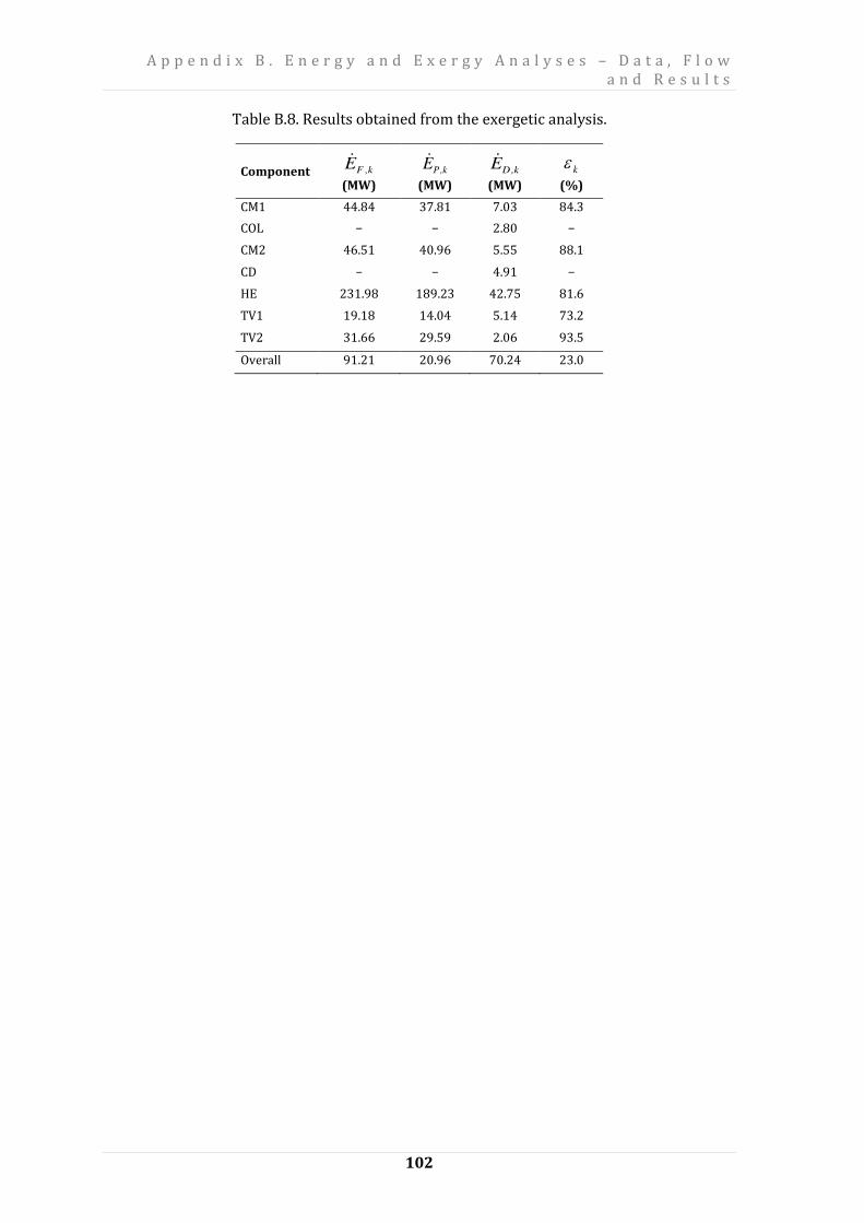
A p p e n d i x B . E n e r g y a n d E x e r g y A n a l y s e s – D a t a , F l o w a n d R e s u l t s
102
Table B.8. Results obtained from the exergetic analysis.
Component k,FE
(MW)
k,PE
(MW)
k,DE
(MW)
kε
(%)
CM1 44.84 37.81 7.03 84.3
COL − − 2.80 −
CM2 46.51 40.96 5.55 88.1
CD − − 4.91 −
HE 231.98 189.23 42.75 81.6
TV1 19.18 14.04 5.14 73.2
TV2 31.66 29.59 2.06 93.5
Overall
91.21 20.96 70.24 23.0

A p p e n d i x B . E n e r g y a n d E x e r g y A n a l y s e s – D a t a , F l o w a n d R e s u l t s
103
B.3 C3MR Process [73]
Table B.9. Composition for the C3MR process mixed-refrigerant in molar percentage.
Component Formula
Mole fraction (%)
Mixed-refrigerant
Natural gas
Methane CH4 41.8 87.5
Ethane C2H6 29.9 5.5
Propane C3H8 21.3 2.1
N-Butane C4H10 - 0.5
I-Butane C4H10 - 0.3
Nitrogen N2 7.0 4.1
Table B.10. LMR and HMR compositions.
Component Formula Mixed-refrigerant (% mol)
LMR HMR
Methane CH4 66.6 28.0
Ethane C2H6 14.9 38.2
Propane C3H8 3.4 31.3
Nitrogen N2 15.1 2.5
Table B.11. Boiling temperatures (in C) for refrigerants at different pressures [104].
Methane Ethane Propane Nitrogen
1 bar -161.7 -89.1 -42.2 -195.9
3 bar -146.5 -66 -13.9 -185.3
6 bar -134.5 -47.9 8.2 -176.8
19 bar -108.7 -9.3 54.8 -158.5
22 bar -104.7 -3.5 61.8 -155.8
Table B.12. Stream 7 molar fraction and its partial pressures
Component Mixed-
refrigerant (% mol)
Partial pressure
(bar)
Methane 41.8 17.82 Ethane 29.9 12.75
Propane 21.3 9.08
Nitrogen 7.0 2.98

A p p e n d i x B . E n e r g y a n d E x e r g y A n a l y s e s – D a t a , F l o w a n d R e s u l t s
104
Table B.13. Enthalpy and Entropy Values Required for Exergy Calculation. S
tre
am
Ma
teri
al
Str
ea
m
T
(K)
P
(bar)
hj (kJ/kg) sj (kJ/kg.K) ���� ���� ���� ���� ���� ����
1
Mix
ed
-re
frig
era
nt
238.57 2.82 -3009.96 -2906.56 -2903.83 -5.62 -5.23 -4.91
2A 300.95 7.50 -2908.57 -2913.78 -2903.83 -5.53 -5.55 -4.91
2B 361.72 17.50 -2800.92 -2930.20 -2903.83 -5.46 -5.85 -4.91
2C 305.00 17.33 -2916.40 -2929.91 -2903.83 -5.80 -5.85 -4.91
2D 382.27 48.60 -2788.57 -2993.79 -2903.83 -5.72 -6.32 -4.91
3 305.00 48.20 -2974.43 -2992.80 -2903.83 -6.26 -6.32 -4.91
4 291.00 46.74 -3032.58 -2989.24 -2903.83 -6.45 -6.30 -4.91
5 279.00 45.33 -3108.24 -2985.87 -2903.83 -6.71 -6.28 -4.91
6 257.00 43.96 -3228.68 -2982.65 -2903.83 -7.15 -6.26 -4.91
7 240.00 42.63 -3307.31 -2979.59 -2903.83 -7.46 -6.25 -4.91
8 240.00 42.63 -3319.20 -3187.16 -3143.89 -5.96 -5.47 -3.87
9 146.00 41.34 -3822.78 -3185.78 -3143.89 -8.57 -5.45 -3.87
10 134.00 40.09 -3860.07 -3184.45 -3143.89 -8.83 -5.44 -3.87
11 118.04 3.00 -3860.07 -3145.89 -3143.89 -8.72 -4.31 -3.87
12 125.98 2.91 -3743.54 -3145.80 -3143.89 -7.77 -4.29 -3.87
13 135.13 2.91 -3605.33 -2906.69 -2903.83 -8.85 -5.24 -4.91
14 240.00 42.63 -3302.76 -3000.20 -2812.01 -8.04 -6.92 -5.37
15 146.00 41.34 -3552.42 -2992.40 -2812.01 -9.35 -6.89 -5.37
16 141.34 2.91 -3552.42 -2815.42 -2812.01 -9.29 -5.67 -5.37
17
Pro
pa
ne
, C3H
8
331.52 14.30 -2351.54 -2742.93 -2376.42 -6.50 -7.74 -6.11
18 305.00 14.30 -2722.83 -2742.93 -2376.42 -7.68 -7.74 -6.11
19 287.34 7.20 -2722.83 -2393.78 -2376.42 -7.67 -6.52 -6.11
20 287.34 7.20 -2675.58 -2393.78 -2376.42 -7.50 -6.52 -6.11
21 287.34 7.20 -2773.09 -2393.78 -2376.42 -7.84 -6.52 -6.11
22 275.45 5.10 -2773.09 -2387.45 -2376.42 -7.84 -6.44 -6.11
23 275.45 5.10 -2687.94 -2387.45 -2376.42 -7.53 -6.44 -6.11
24 275.45 5.10 -2805.09 -2387.45 -2376.42 -7.95 -6.44 -6.11
25 253.91 2.50 -2805.09 -2380.27 -2376.42 -7.94 -6.29 -6.11
26 253.91 2.50 -2600.62 -2380.27 -2376.42 -7.14 -6.29 -6.11
27 253.91 2.50 -2859.76 -2380.27 -2376.42 -8.16 -6.29 -6.11
28 237.14 1.30 -2859.76 -2377.15 -2376.42 -8.15 -6.16 -6.11
29 238.50 1.30 -2471.73 -2377.15 -2376.42 -6.51 -6.16 -6.11
30 265.42 2.50 -2434.22 -2380.27 -2376.42 -6.48 -6.29 -6.11
31 258.13 2.50 -2445.80 -2380.27 -2376.42 -6.53 -6.29 -6.11
32 289.34 5.10 -2402.76 -2387.45 -2376.42 -6.49 -6.44 -6.11
33 285.07 5.10 -2410.09 -2387.45 -2376.42 -6.52 -6.44 -6.11
34 301.12 7.20 -2388.42 -2393.78 -2376.42 -6.50 -6.52 -6.11
35 297.41 7.20 -2395.10 -2393.78 -2376.42 -6.53 -6.52 -6.11
36 287.34 7.20 -2413.10 -2393.78 -2376.42 -6.59 -6.52 -6.11
37 275.45 5.10 -2426.45 -2387.45 -2376.42 -6.58 -6.44 -6.11
38 253.91 2.50 -2452.42 -2380.27 -2376.42 -6.55 -6.29 -6.11

A p p e n d i x B . E n e r g y a n d E x e r g y A n a l y s e s – D a t a , F l o w a n d R e s u l t s
105
Fig. B.4. C3MR flowsheet using Aspen Plus [73].
NG
LNG
Liquefaction and
Sub-cooling Block
Pre-cooling
Block
Legend:
Natural Gas LNG refrigerant (Propane) mixed-refrigerant mixed-refrigerant (gas) mixed-refrigerant (liquid)
Final Product

A p p e n d i x B . E n e r g y a n d E x e r g y A n a l y s e s – D a t a , F l o w a n d R e s u l t s
106
Table B.14. Thermodynamic data for the material streams at real operating conditions for
C3MR process [73].
Str
ea
m
Ma
teri
al
stre
am
m T p x TE
ME
PHE
(kg/s) (°K) (bar) (kg/kg) (kW) (kW) (kW)
1 M
ixe
d R
efr
ige
ran
t 301.84 238.57 2.82 1.00 3556.46 28059.29 31615.75
2A 301.84 300.95 7.50 1.00 7.34 54453.44 54460.77
2B 301.84 361.72 17.50 1.00 3691.12 76447.38 80138.51
2C 301.84 305.00 17.33 1.00 46.17 76202.22 76248.39
2D 301.84 382.27 48.60 1.00 7234.19 99939.58 107173.77
3 301.84 305.00 48.20 1.00 62.28 99775.23 99837.51
4 301.84 291.00 46.74 0.91 185.95 99158.24 99344.20
5 301.84 279.00 45.33 0.73 1315.82 98535.69 99851.51
6 301.84 257.00 43.96 0.50 5553.83 97904.16 103457.98
7 301.84 240.00 42.63 0.36 10572.31 97264.45 107836.77
8 83.58 240.00 42.63 1.00 1273.96 36167.88 37441.84
9 83.58 146.00 41.34 0.00 24425.44 35890.78 60316.22
10 83.58 134.00 40.09 0.00 28179.01 35613.12 63792.13
11 83.58 118.04 3.00 0.18 50361.68 10719.10 61080.78
12 83.58 125.98 2.91 0.45 36602.91 10419.07 47021.97
13 301.84 135.13 2.91 0.22 113993.78 28915.64 142909.43
14 218.27 240.00 42.63 0.00 6465.87 59991.16 66457.03
15 218.27 146.00 41.34 0.00 37406.26 59706.93 97113.19
16 218.27 141.34 2.91 0.08 75098.15 18480.75 93578.90
17
Pro
pa
ne
, C3H
8
442.70 331.52 14.30 1.00 8842.63 52910.10 61752.73
18 442.70 305.00 14.30 0.00 101.36 52910.10 53011.46
19 442.70 287.34 7.20 0.14 5317.29 46310.07 51627.36
20 442.70 287.34 7.20 0.27 4530.45 46310.07 50840.52
21 322.79 287.34 7.20 0.00 4487.48 33766.25 38253.74
22 322.79 275.45 5.10 0.08 9723.92 28144.07 37867.99
23 322.79 275.45 5.10 0.31 7458.59 28144.07 35602.66
24 222.92 275.45 5.10 0.00 7303.29 19436.79 26740.08
25 222.92 253.91 2.50 0.13 15003.73 11026.38 26030.11
26 222.92 253.91 2.50 0.64 7062.21 11026.38 18088.59
27 81.10 253.91 2.50 0.00 6231.08 4011.54 10242.61
28 81.10 237.14 1.30 0.09 8964.84 1115.87 10080.71
29 81.10 238.50 1.30 1.00 869.21 1115.87 1985.07
30 81.10 265.42 2.50 1.00 256.38 4011.54 4267.92
31 222.92 258.13 2.50 1.00 1063.50 11026.38 12089.87
32 222.92 289.34 5.10 1.00 51.34 19436.79 19488.13
33 322.79 285.07 5.10 1.00 164.53 28144.07 28308.60
34 322.79 301.12 7.20 1.00 8.59 33766.25 33774.84
35 442.70 297.41 7.20 1.00 0.77 46310.07 46310.85
36 119.91 287.34 7.20 1.00 42.97 12543.82 12586.78
37 99.87 275.45 5.10 1.00 155.30 8707.28 8862.58

A p p e n d i x B . E n e r g y a n d E x e r g y A n a l y s e s – D a t a , F l o w a n d R e s u l t s
107
38 141.82 253.91 2.50 1.00 831.14 7014.84 7845.99
39
Na
tura
l G
as
158.42 300.00 65.00 1.00 2.36 86893.82 86896.18
40 158.42 291.00 63.05 1.00 35.98 86316.80 86352.77
41 158.42 279.00 61.16 1.00 267.99 85738.21 86006.20
42 158.42 257.00 59.33 1.00 1360.82 85158.73 86519.55
43 158.42 240.00 57.55 1.00 3002.05 84575.73 87577.78
44 158.42 146.00 55.82 0.00 48032.84 83989.62 132022.46
45 158.42 134.00 54.15 0.00 55971.06 83404.49 139375.55
46 158.42 113.15 1.22 0.18 127682.63 3918.38 131601.01
47 28.71 113.15 1.22 1.00 5427.65 711.13 6138.77
LNG LNG 129.71 113.15 1.22 0.00 121075.46 3207.19 124282.65
Table B.15. Standard Molar Chemical Exergy Values for Selected Substances at Tref =
298.15K. Model II is referred.
Substance Formula �� �
(kJ/kmol)
Propane C3H8 (g) 2154000
Nitrogen N2 (g) 720
Methane CH4 (g) 831650
Ethane C2H6 (g) 1495840
Table B.16. Chemical exergy result for affected streams for C3MR
Stream 7 8 12 13 14 16 � � (GW) 13.96 3.39 3.39 13.96 10.57 10.57

A p p e n d i x B . E n e r g y a n d E x e r g y A n a l y s e s – D a t a , F l o w a n d R e s u l t s
108
Table B.17. Definition of the exergy of fuel and the exergy of product for the components of the C3MR process.
Component � , ��,
HEX1** � = �� + �� + �� − � �+ �� − � �+ �� − � �+ ��� − �� � �� = �� + ��
HEX2 � = ��� − �� � + �� − � � + �� − � �+ �� − � � �� = ��� − ���+ ��� − �� �
HEX3 � = ��� − �� � + �� − � �+ �� − � �+ �� − � � �� = ��� − ��� + ��� − �� �
HEX4 � = ��� − �� � + �� − � � + �� − � � + �� − � � �� = ��� − ���+ ��� − �� �
MLHE1 � = ��� − ���+ �� − � � + �� − � �+ �� − � �
+ �� − � �
�� = ��� − �� �+ ��� − ��� + ��� − �� �
MLHE2 � = ��� − �� �+ �� − � � + �� − � � + �� − � � �� = ��� − ��� + ��� − �� �
COMP1 � = ��� − �� �+ � � � �� = �� − � �
COMP2 � = ��� − �� �+ � � � �� = �� − � �
COMP3** � = �� + � � � �� = �� − � � + ��
COMP4 � = �� + � � � �� = �� − � � + ��
COMP5 � = �� + � � � �� = �� − � �+ ��
COMP6 � = � � � �� = ��� − �� �+ �� − � �
COMP7 � = � � � �� = ��� − �� �+ �� − � �
** Components crossing the environmental temperature

A p p e n d i x B . E n e r g y a n d E x e r g y A n a l y s e s – D a t a , F l o w a n d R e s u l t s
109
MIX1 � = � ∗ � + � ∗ ( � − � ) �� = � ∗ �
MIX2 � = � ∗ ( � − � ) �� = � ∗ ( � − � )
MIX3 � = � ∗ ( � − � ) �� = � ∗ ( � − � )
MIX4 � = � ∗ ( � − � ) + � ∗ ( � − �) + � ∗ ( − ) �� = � ∗ ( � − � ) + � ∗ ( � − �) + � ∗ ( − )
VALVE1 � = �� − � � �� = ��� − �� �
VALVE2 � = �� − � � �� = ��� − �� �
VALVE3 � = �� − � � �� = ��� − �� �
VALVE4** � = �� − � �+ �� �� = ��� �
VALVE5 � = �� − � � �� = ��� − �� �
VALVE6 � = �� − � � �� = ��� − �� �
Overall system
� ,������ = ������������� ��,������ = � − �
** Components crossing the environmental temperature

A p p e n d i x B . E n e r g y a n d E x e r g y A n a l y s e s – D a t a , F l o w a n d R e s u l t s
110
Table B.18. Exergy rate of product and fuel for the selected components of the C3MR process
Component
,
(MW)
�,
(MW)
,
(MW)
� (%)
� ,
(%)
HEX1 2.05 0.22 1.82 10.85 1.17
HEX2 3.47 1.36 2.1 39.29 1.35
HEX3 9.15 5.33 3.82 58.24 2.45
HEX4 9.32 6.66 2.66 71.47 1.7
MLHE1 112.44 99.12 13.32 88.16 8.53
MLHE2 14.92 11.69 3.23 78.35 2.07
COMP1 3.99 2.90 1.1 72.52 0.7
COMP2 11.67 8.41 3.26 72.05 2.09
COMP3 7.94 5.63 2.31 70.92 1.48
COMP4 21.43 15.44 5.99 72.07 3.83
COMP5 37.56 26.40 11.16 70.29 7.14
COMP6 36.11 25.68 10.43 71.12 6.68
COMP7 42.87 30.93 11.95 72.13 7.65
Total System 156.22 52.48 103.74*) 33.59 66.41
*) Throttling valves and mixers as well as coolers (dissipative components) are included

A p p e n d i x B . E n e r g y a n d E x e r g y A n a l y s e s – D a t a , F l o w a n d R e s u l t s
111
B.4 AP-XTM Process [51]
Fig. B.5. A general schematic on the AP-X process.
Table B.19. Composition for the AP-X process in molar percentage.
Component Formula Mole fraction (%)
Natural
Mixed Refrigerant Nitrogen N2 0.1 1.4
Methane CH4 86.0 34.3
Ethane C2H6 7.5 39.5
Propane C3H8 3.5 0.6
I-Butane C4H10 1.0 9.1
Butane C4H10 1.0 15.1
I-Pentane C5H12 0.3 -
Pentane C5H12 0.2 -
Hexane C6H14 0.4 -

A p p e n d i x B . E n e r g y a n d E x e r g y A n a l y s e s – D a t a , F l o w a n d R e s u l t s
112
Fig. B.6. Flowsheet for AP-XTM process.

A p p e n d i x B . E n e r g y a n d E x e r g y A n a l y s e s – D a t a , F l o w a n d R e s u l t s
113
Fig. B.7. �- T diagram for HEX0 (∆ ����ℎ = 0.3�)
Fig. B.8. �- T diagram for HEX1 (∆ ����ℎ = 6.4�)
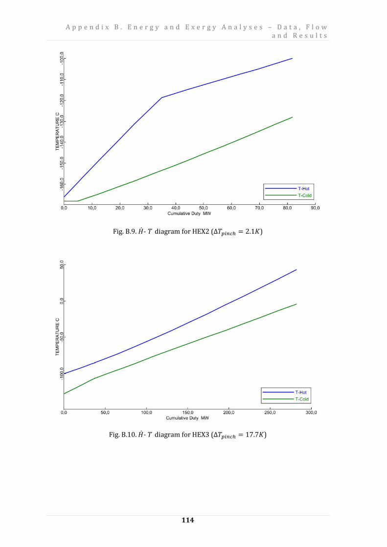
A p p e n d i x B . E n e r g y a n d E x e r g y A n a l y s e s – D a t a , F l o w a n d R e s u l t s
114
Fig. B.9. �- T diagram for HEX2 (∆ ����ℎ = 2.1�)
Fig. B.10. �- T diagram for HEX3 (∆ ����ℎ = 17.7�)

A p p e n d i x B . E n e r g y a n d E x e r g y A n a l y s e s – D a t a , F l o w a n d R e s u l t s
115
Table B.20. Thermodynamic data for the material streams at real operating conditions.
Stream
Ma
teri
al
Str
ea
m
(kg/s) T
(°C) P
(bar) x
ET (MW)
EM (MW)
EPH (MW)
1 N
atu
ral
Ga
s 224.23 43.00 65.00 0.00 0.00 121.85 121.85
2 224.23 17.85 65.00 0.00 0.64 121.85 122.49
3 224.23 7.00 65.00 0.01 1.53 121.85 123.37
4 224.23 -16.15 65.00 0.06 4.97 121.85 126.82
5 224.23 -33.15 65.00 0.12 9.48 121.85 131.32
6 224.23 -85.00 65.00 1.00 43.05 121.85 164.90
7 224.23 -111.00 65.00 1.00 60.43 121.85 182.27
8 224.23 -166.00 4.51 1.00 188.16 44.95 233.12
9 224.23 -165.84 1.05 1.00 231.58 1.06 232.64
10 224.23 -165.84 1.05 1.00 231.58 1.06 232.64
11
97
Mix
ed
-re
frig
era
nt
7000.00 65.00 38.00 0.00 26.82 1913.78 1940.60
98 7000.00 60.00 38.00 0.02 19.76 1913.78 1933.54
99 7000.00 55.00 38.00 0.08 9.76 1913.78 1923.54
100 7000.00 45.00 38.00 0.20 0.47 1913.78 1914.25
101 5062.25 45.00 38.00 0.00 0.33 1575.49 1575.82
102 1937.75 45.00 38.00 1.00 0.37 292.91 293.29
103 1937.75 -55.00 38.00 1.00 90.45 293.05 383.50
104 1937.75 -54.27 10.00 0.99 128.59 240.94 369.53
105 1937.75 28.57 10.00 0.52 5.30 240.94 246.24
106 6792.45 15.69 10.00 0.06 36.51 1235.37 1271.87
107 7000.00 14.57 10.00 0.07 42.20 1278.02 1320.22
107A 7000.00 42.18 21.00 0.01 0.60 1659.77 1660.36
107B 7000.00 40.00 19.45 0.01 0.57 1622.41 1622.98
107C 6897.81 40.00 19.45 0.00 0.17 1608.24 1608.42
108 6897.81 84.46 38.00 0.00 54.91 1899.65 1954.56
109 102.19 40.00 19.45 1.00 0.00 10.75 10.75
110 102.19 41.74 38.00 1.00 0.00 11.16 11.16
111 7000.00 82.41 38.00 0.00 53.42 1913.78 1967.19
112 5062.25 -100.00 38.00 1.00 881.43 1575.49 2456.92
113 5062.25 -111.00 34.50 1.00 1041.92 1540.12 2582.04
114 4854.70 -110.95 33.46 1.00 1008.19 1466.11 2474.30
115 4854.70 -111.37 10.00 0.98 1441.86 989.74 2431.60
116 4854.70 -105.00 10.00 0.90 1286.21 989.74 2275.94
117 4854.70 28.57 10.00 0.00 3.31 989.74 993.05
118 207.55 -110.95 33.46 1.00 43.10 62.68 105.78
119 207.55 -111.37 10.00 0.98 61.64 42.31 103.96

A p p e n d i x B . E n e r g y a n d E x e r g y A n a l y s e s – D a t a , F l o w a n d R e s u l t s
116
120 207.55 -34.05 10.00 0.28 11.42 42.31 53.73
500
Pro
pa
ne
4000.00 17.58 7.90 0.89 117.69 467.50 585.19
501 4000.00 17.58 7.90 0.66 90.24 467.50 557.74
502 2658.31 17.58 7.90 1.00 87.65 310.69 398.33
503 2658.31 6.61 5.80 0.92 128.88 266.42 395.30
504 2658.31 6.61 5.80 0.78 110.63 266.42 377.05
505 2069.74 6.61 5.80 1.00 108.31 207.43 315.74
506 2069.74 -17.09 2.70 0.85 189.04 118.33 307.37
507 2069.74 -17.09 2.70 0.55 130.90 118.33 249.23
508 1145.35 -17.09 2.70 1.00 120.97 65.48 186.45
509 1145.35 -36.01 1.30 0.89 166.57 16.83 183.41
510 1145.35 -36.01 1.30 0.00 21.53 16.83 38.36
511 1145.35 20.49 5.00 0.00 1.68 105.44 107.12
512 2069.74 1.82 2.70 0.00 10.04 118.33 128.37
513 2069.74 61.49 10.00 0.00 2.05 267.27 269.32
514 2658.31 45.45 5.80 0.00 0.09 266.42 266.51
515 2658.31 91.57 15.00 0.00 20.12 394.49 414.61
516 4000.00 62.51 7.90 0.00 4.47 467.50 471.96
517 4000.00 109.12 20.00 0.00 100.52 598.40 698.93
518 4000.00 31.85 20.00 1.00 2.29 598.40 600.70
519 1341.69 17.58 7.90 0.00 2.62 156.81 159.43
520 588.57 6.61 5.80 0.00 2.34 58.99 61.33
521 924.39 -17.09 2.70 0.00 9.82 52.85 62.67
1000
Nit
rog
en
1510.00 -149.70 11.00 0.00 179.57 338.02 517.59
1001 1510.00 -34.05 11.00 0.00 18.16 338.02 356.17
1001A 1510.00 30.60 21.00 0.00 0.41 429.80 430.20
1001B 1510.00 40.00 21.00 0.00 0.02 429.80 429.82
1001C 1510.00 137.99 44.00 0.00 19.61 535.07 554.68
1001D 1510.00 40.00 44.00 0.00 0.02 535.07 535.10
1002 1510.00 93.10 67.00 0.00 6.09 595.27 601.36
1003 1510.00 43.00 67.00 0.00 0.00 595.27 595.27
1004 1510.00 -100.00 67.00 0.00 0.00 621.61 621.61
1005 1510.00 -168.04 11.00 0.02 255.74 338.02 593.76

A p p e n d i x B . E n e r g y a n d E x e r g y A n a l y s e s – D a t a , F l o w a n d R e s u l t s
117
Table B.21. Mole flow rate of the mixed refrigerant.
Component Nitrogen Methane Ethane Propane iButane Butane
Total stream (kmol/s)
100 3.05 74.79 86.13 1.31 19.84 32.93
101 2.96 70.69 72.80 0.92 11.13 16.67
102 0.09 4.10 13.33 0.39 8.71 16.25
103 0.09 4.10 13.33 0.39 8.71 16.25
104 0.09 4.10 13.33 0.39 8.71 16.25
105 0.09 4.10 13.33 0.39 8.71 16.25
106 2.93 71.89 83.14 1.27 19.39 32.24
107 3.05 74.79 86.13 1.31 19.84 32.93
107A 3.05 74.79 86.13 1.31 19.84 32.93
107B 3.05 74.79 86.13 1.31 19.84 32.93
107C 3.05 74.71 85.76 1.29 19.36 31.88
108 3.05 74.71 85.76 1.29 19.36 31.88
109 0.00 0.08 0.37 0.02 0.49 1.05
110 0.00 0.08 0.37 0.02 0.49 1.05
111 3.05 74.79 86.13 1.31 19.84 32.93
112 2.96 70.69 72.80 0.92 11.13 16.67
113 2.96 70.69 72.80 0.92 11.13 16.67
114 2.84 67.80 69.81 0.88 10.67 15.99
115 2.84 67.80 69.81 0.88 10.67 15.99
116 2.84 67.80 69.81 0.88 10.67 15.99
117 2.84 67.80 69.81 0.88 10.67 15.99
118 0.12 2.90 2.98 0.04 0.46 0.68
119 0.12 2.90 2.98 0.04 0.46 0.68
120 0.12 2.90 2.98 0.04 0.46 0.68
Vapor phase (kmol/s)
100 2.96 70.69 72.80 0.92 11.13 16.67
101 2.96 70.69 72.80 0.92 11.13 16.67
102 0.00 0.00 0.00 0.00 0.00 0.00
103 0.00 0.00 0.00 0.00 0.00 0.00
104 0.02 0.29 0.06 0.00 0.00 0.00
105 0.09 3.84 10.05 0.19 2.52 3.76
106 2.93 71.60 81.24 1.17 16.02 24.92
107 3.05 74.45 83.86 1.19 15.93 24.49
107A 3.05 74.68 85.62 1.29 19.20 31.56
107B 3.05 74.71 85.76 1.29 19.36 31.88
107C 3.05 74.71 85.76 1.29 19.36 31.88
108 3.05 74.71 85.76 1.29 19.36 31.88
109 0.00 0.00 0.00 0.00 0.00 0.00
110 0.00 0.00 0.00 0.00 0.00 0.00
111 3.05 74.79 86.13 1.31 19.84 32.93
112 0.00 0.00 0.00 0.00 0.00 0.00
113 0.00 0.00 0.00 0.00 0.00 0.00
114 0.00 0.00 0.00 0.00 0.00 0.00
115 0.60 2.42 0.04 0.00 0.00 0.00

A p p e n d i x B . E n e r g y a n d E x e r g y A n a l y s e s – D a t a , F l o w a n d R e s u l t s
118
116 1.85 14.74 0.40 0.00 0.00 0.00
117 2.84 67.80 69.81 0.88 10.67 15.99
118 0.00 0.00 0.00 0.00 0.00 0.00
119 0.03 0.10 0.00 0.00 0.00 0.00
120 0.12 2.80 2.14 0.01 0.05 0.05
Liquid phase (kmol/s)
100 0.09 4.10 13.33 0.39 8.71 16.25
101 0.00 0.00 0.00 0.00 0.00 0.00
102 0.09 4.10 13.33 0.39 8.71 16.25
103 0.09 4.10 13.33 0.39 8.71 16.25
104 0.07 3.80 13.27 0.39 8.71 16.25
105 0.00 0.25 3.28 0.20 6.19 12.50
106 0.00 0.29 1.90 0.10 3.36 7.32
107 0.01 0.34 2.27 0.12 3.91 8.44
107A 0.00 0.11 0.51 0.02 0.64 1.37
107B 0.00 0.08 0.37 0.02 0.49 1.05
107C 0.00 0.00 0.00 0.00 0.00 0.00
108 0.00 0.00 0.00 0.00 0.00 0.00
109 0.00 0.08 0.37 0.02 0.49 1.05
110 0.00 0.08 0.37 0.02 0.49 1.05
111 0.00 0.00 0.00 0.00 0.00 0.00
112 2.96 70.69 72.80 0.92 11.13 16.67
113 2.96 70.69 72.80 0.92 11.13 16.67
114 2.84 67.80 69.81 0.88 10.67 15.99
115 2.24 65.38 69.77 0.88 10.67 15.99
116 0.99 53.06 69.42 0.88 10.67 15.99
117 0.00 0.00 0.00 0.00 0.00 0.00
118 0.12 2.90 2.98 0.04 0.46 0.68
119 0.10 2.80 2.98 0.04 0.46 0.68
120 0.00 0.10 0.85 0.03 0.40 0.63
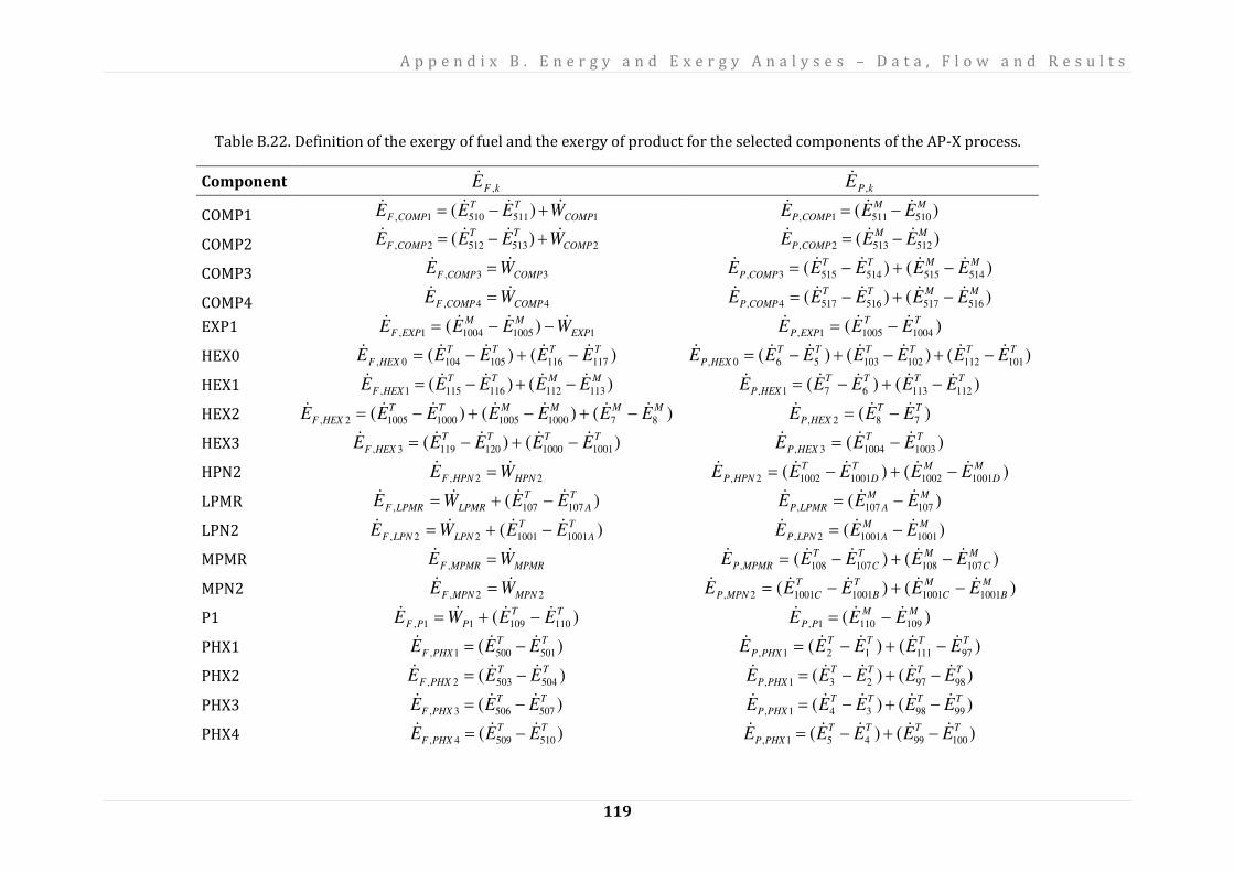
A p p e n d i x B . E n e r g y a n d E x e r g y A n a l y s e s – D a t a , F l o w a n d R e s u l t s
119
Table B.22. Definition of the exergy of fuel and the exergy of product for the selected components of the AP-X process.
Component kFE , kPE ,
COMP1 15115101, )( COMP
TT
COMPF WEEE +−= )( 5105111,
MM
COMPP EEE −=
COMP2 25135122, )( COMP
TT
COMPF WEEE +−= )( 5125132,
MM
COMPP EEE −=
COMP3 33, COMPCOMPF WE = )()( 5145155145153,
MMTT
COMPP EEEEE −+−=
COMP4 44, COMPCOMPF WE = )()( 5165175165174,
MMTT
COMPP EEEEE −+−=
EXP1 1100510041, )( EXP
MM
EXPF WEEE −−= )( 100410051,
TT
EXPP EEE −=
HEX0 )()( 1171161051040,
TTTT
HEXF EEEEE −+−= )()()( 101112102103560,
TTTTTT
HEXP EEEEEEE −+−+−=
HEX1 )()( 1131121161151,
MMTT
HEXF EEEEE −+−= )()( 112113671,
TTTT
HEXP EEEEE −+−=
HEX2 )()()( 8710001005100010052,
MMMMTT
HEXF EEEEEEE −+−+−= )( 782,
TT
HEXP EEE −=
HEX3 )()( 100110001201193,
TTTT
HEXF EEEEE −+−= )( 100310043,
TT
HEXP EEE −=
HPN2 22, HPNHPNF WE = )()( 10011002100110022,
M
D
MT
D
T
HPNP EEEEE −+−=
LPMR )( 107107,
T
A
T
LPMRLPMRF EEWE −+= )( 107107,
MM
ALPMRP EEE −=
LPN2 )( 1001100122,
T
A
T
LPNLPNF EEWE −+= )( 100110012,
MM
ALPNP EEE −=
MPMR MPMRMPMRF WE =, )()( 107108107108,
M
C
MT
C
T
MPMRP EEEEE −+−=
MPN2 22, MPNMPNF WE = )()( 10011001100110012,
M
B
M
C
T
B
T
CMPNP EEEEE −+−=
P1 )( 11010911,
TT
PPF EEWE −+= )( 1091101,
MM
PP EEE −=
PHX1 )( 5015001,
TT
PHXF EEE −= )()( 97111121,
TTTT
PHXP EEEEE −+−=
PHX2 )( 5045032,
TT
PHXF EEE −= )()( 9897231,
TTTT
PHXP EEEEE −+−=
PHX3 )( 5075063,
TT
PHXF EEE −= )()( 9998341,
TTTT
PHXP EEEEE −+−=
PHX4 )( 5105094,
TT
PHXF EEE −= )()( 10099451,
TTTT
PHXP EEEEE −+−=

A p p e n d i x B . E n e r g y a n d E x e r g y A n a l y s e s – D a t a , F l o w a n d R e s u l t s
120
PSEP1 )( 5015011,
MT
PSEPF EEE +=
)()( 5195025195021,
MMTT
PSEPP EEEEE +++=
PSEP2 )( 5045042,
MT
PSEPF EEE +=
)()( 5205055205052,
MMTT
PSEPP EEEEE +++=
PSEP3 )( 5075073,
MT
PSEPF EEE +=
)()( 5215085215082,
MMTT
PSEPP EEEEE +++=
PV1 )( 5035021,
MM
PVF EEE −=
)( 5025031,
TT
PVP EEE −=
PV2 )( 5065052,
MM
PVF EEE −=
)( 5055062,
TT
PVP EEE −=
PV3 )( 5095083,
MM
PVF EEE −=
)( 5085093,
TT
PVP EEE −=
PV4 )( 5005184,
MM
PVF EEE −=
)( 5185004,
TT
PVP EEE −=
SEP2 )( 1001002,
MT
SEPF EEE +=
)()( 1021011021012,
MMTT
SEPP EEEEE +++=
SEP3 )( 1071073,
M
B
T
BSEPF EEE +=
)()( 1091071091073,
MM
C
TT
CSEPP EEEEE +++=
V0 )( 1041030,
MM
VF EEE −=
)( 1031040,
TT
VP EEE −=
V1 )( 1151141,
MM
VF EEE −=
)( 1141151,
TT
VP EEE −=
V2 )( 1191182,
MM
VF EEE −=
)( 1181192,
TT
VP EEE −=
V3 )( 983,
MM
VF EEE −=
)( 893,
TT
VP EEE −=
Total System
� ,������ = ������������� ��,������ = � − �
Note: Dissipative components are mixers, coolers, after- and intercoolers. Separator SEP1 has no flash product thus not considered.

A p p e n d i x B . E n e r g y a n d E x e r g y A n a l y s e s – D a t a , F l o w a n d R e s u l t s
121
Table B.23. Exergy rate of product and fuel for the AP-X process.
Component
,
(MW)
�,
(MW)
,
(MW)
� (%)
COMP1 120.5 88.6 31.9 74
COMP2 206.5 148.9 57.5 72
COMP3 223.8 128.1 95.8 57
COMP4 404.9 130.9 274.0 32
EXP1 283.6 188.8 94.8 67
HEX0 1406.2 1004.7 401.4 71
HEX1 191.0 177.9 13.2 93
HEX2 153.1 127.7 25.3 83
HEX3 211.6 0.0 211.6 0
HPN2 100.4 60.2 40.2 60
LPMR 546.0 381.8 164.2 70
LPN2 130.0 91.8 38.2 71
MPMR 550.1 291.4 258.7 53
MPN2 192.6 105.3 87.3 55
P1 0.5 0.4 0.0 89
PHX1 27.5 27.2 0.2 99
PHX2 18.2 7.9 10.3 44
PHX3 58.1 13.4 44.7 23
PHX4 145.0 13.8 131.2 10
Overall System 2024.7 111.27 2013.41*) 6
*) Throttling valves and mixers as well as coolers (dissipative components) are included

A p p e n d i x B . E n e r g y a n d E x e r g y A n a l y s e s – D a t a , F l o w a n d R e s u l t s
122
Table B.24. Power net required by AP-X process components.
Components Power (MW)
COMP1 100.70
COMP2 198.48
COMP3 203.82
COMP4 308.88
EXP1 -66.93
HPN2 94.35
LPMR 504.36
LPN2 112.23
MPMR 495.35
MPN2 173.00
P1 0.45

A p p e n d i x B . E n e r g y a n d E x e r g y A n a l y s e s – D a t a , F l o w a n d R e s u l t s
123
As of 2013, the AP-XTM process has been utilized in the liquefaction plant at 12% in capacity
worldwide, as per Fig. 1.4. This coverage does not include Malaysia. However, PETRONAS’
new floating LNG (PFLNG 1) process namely AP-NTM uses AP-XTM as its reference design
[105].
Fig. B.11. PETRONAS FLNG to be commissioned in 2015 [15].

A p p e n d i x B . E n e r g y a n d E x e r g y A n a l y s e s – D a t a , F l o w a n d R e s u l t s
124
B.5 MR-X Process [56,94]
Table B.25. Composition of NG and refrigerants for MR-X process.
Component Formula
Mole Fraction (%)
Natural Gas
Pre-cooling
Liquefaction Sub-
cooling
Nitrogen N2 0.1
1.4 100.0
Methane CH4 86.0
34.3
Ethane C2H6 7.5 45.5 39.5
Propane C3H8 3.5 4.9 0.6
I-Butane C4H10-2 1.0
9.1
Butane C4H10-1 1.0 49.6 15.1
I-Pentane C5H12-2 0.3
Pentane C5H12-1 0.2
Hexane C6H14-1 0.4
Legend:
natural gas L N G mixed-refrigerant nitrogen for pre-cooling block for sub-cooling block mixed refrigerant gas phase liquid phase of mixed refrigerant of mixed refrigerant
Fig. B.12. A general schematic on the MR-X process.

A p p e n d i x B . E n e r g y a n d E x e r g y A n a l y s e s – D a t a , F l o w a n d R e s u l t s
125
V1
HEX2
EXP1
V3
V2
HEX3
AC
SEP2
HEX0
V0
HEX1
SEP1
P1
MIX3
MIX2
MIX1
S1
HPN2
LPMR
ICMR
SEP3
MPMR
IC2
LPN2 MPN2
PHE2
PHE1
PS1
PV1
PM1
PV2
PC1
PAC
IC1
PC2
114
115
5
10056
1000 1004
7
118
119
1003
1001
120
1002
100
101
102
3
104
116
105117
103
1124
113
9
8
109
110
108
106
107
1001D
107A
107B
107C
1001C1001A
204
2
207
206
208
205
1
201
202
210
203209 211
1001B
111
212
99
NG
Flash gas
COLDBOX
LNG
Legend:
NG-LNG
Mixed-refrigerant for main
liquefaction section
Mixed-refrigerant for pre-
cooling section
Nitrogen for sub-cooling
section
Fig. B.13 Process flow diagram for MR-X process

A p p e n d i x B . E n e r g y a n d E x e r g y A n a l y s e s – D a t a , F l o w a n d R e s u l t s
126
Fig. B.14. Cumulative cooling curves for the MR-X process.

A p p e n d i x B . E n e r g y a n d E x e r g y A n a l y s e s – D a t a , F l o w a n d R e s u l t s
127
Table B.26. Thermodynamic data for the material streams (at real operating conditions).
Stream Material
stream
m p T TE
ME
PHE
(kg/s) (bar) (ºC) (MW) (MW) (MW)
1
NG
-LN
G
224.22
65.00 43.00 0.00 121.84 121.84
2 65.00 0.00 2.30 121.84 124.14
3 65.00 -33.15 9.46 121.84 131.31
4 63.05 -85.00 43.46 121.02 164.49
5 61.16 -111.00 61.37 120.22 181.59
6 59.32 -168.00 119.45 119.40 238.85
7 1.05 -165.21 229.77 1.06 230.83
8 1.05 -165.21 229.77 1.06 230.83
99
Ma
in M
ixe
d R
efr
ige
ran
t
958.33 50.00 60.00 2.31 275.11 277.42
100 958.33 50.00 50.00 0.36 275.11 275.47
101 638.36 50.00 50.00 0.29 212.79 213.08
102 319.98 50.00 50.00 0.06 56.91 56.97
103 319.98 48.50 -55.00 15.05 56.79 71.85
104 319.98 10.00 -57.17 25.17 43.23 68.40
105 319.98 10.00 41.84 0.02 43.23 43.25
106 932.16 10.00 33.18 0.32 169.62 169.94
107 958.33 10.00 32.99 0.30 174.97 175.27
107A 958.33 30.00 104.04 12.52 249.29 261.82
107B 958.33 30.00 43.00 0.02 249.29 249.31
107C 769.96 30.00 43.00 0.02 219.20 219.22
108 769.96 50.00 80.24 4.74 244.79 249.53
109 188.37 30.00 43.00 0.00 24.79 24.79
110 188.37 50.00 45.14 0.02 25.63 25.64
111 958.33 50.00 64.89 3.97 275.11 279.08
112 638.36 48.50 -100.00 102.03 211.54 313.57
113 638.36 34.50 -111.00 130.66 196.40 327.06
114 612.18 34.50 -111.00 125.31 188.34 313.65
115 612.18 10.00 -111.75 181.88 126.10 307.98
116 612.18 10.00 -100.02 145.94 126.10 272.04
117 612.18 10.00 41.84 0.01 126.10 126.11
118 26.17 34.50 -111.00 5.36 8.05 13.41
119 26.17 10.00 -111.75 7.78 5.39 13.17
120 26.17 10.00 26.55 0.02 5.39 5.41
1000
Nit
rog
en
649.17
11.00 -118.48 46.10 145.32 191.42
1001 10.67 26.55 0.30 143.46 143.77
1001A 21.00 115.16 4.96 184.77 189.73
1001B 21.00 43.00 0.00 184.77 184.77

A p p e n d i x B . E n e r g y a n d E x e r g y A n a l y s e s – D a t a , F l o w a n d R e s u l t s
128
1001C 44.00 145.93 9.76 230.03 239.79
1001D 44.00 43.00 0.00 230.03 230.03
1002 67.00 98.75 3.20 255.91 259.12
1003 67.00 43.00 0.00 255.91 255.91
1004 64.99 -100.00 43.01 254.03 297.04
1005 11.00 -168.04 107.81 145.32 253.13
201
Pre
-co
oli
ng
Mix
ed
Re
frig
era
nt
500.00 19.00 43.00 0.00 71.90 71.90
202 500.00 19.00 0.00 5.10 71.90 77.00
203 305.00 19.00 0.00 3.11 43.86 46.97
204 195.00 19.00 0.00 1.99 28.04 30.03
205 305.00 8.83 -5.33 9.36 36.82 46.18
206 195.00 19.00 -33.15 5.66 28.04 33.70
207 195.00 3.51 -38.82 19.03 13.87 32.90
208 195.00 3.51 26.35 0.16 13.87 14.03
209 195.00 9.00 67.67 0.43 23.71 24.14
210 305.00 8.83 63.77 0.49 36.82 37.30
211 500.00 8.83 65.22 0.85 60.36 61.20
212 500.00 19.00 102.14 11.94 71.90 83.84

129
Appendix C. Economic Analysis
Data and Flow – A Study Case on
the C3MR Process

A p p e n d i x C . E c o n o m i c A n a l y s i s D a t a a n d F l o w – A S t u d y C a s e o n t h e C 3 M R P r o c e s s
130
C.1 Purchased Equipment Costs (PEC) Estimates
Levelized values of total capital investment (TCI) comprising purchase equipment costs, fuel
costs, and operating and maintenance expenditures for the life span of the liquefaction plant
is assumed to be 20 years (2016-2036). Annually, the average plant capacity factor is
assumed to be 85 %, which means it operates 7446 hrs out of total 8760 hrs available. Table
C.1 presents all considered parameters for the analysis.
Table C.1. Parameters and assumptions used in TRR calculations [62]
Parameter (units) Value
1a. Average general inflation rate (1994-2017) (%) 5.0
b. Average nominal escalation rate of all costs (except fuel) (1994-2017) (%) 5.0
c. Average nominal escalation rate of electricity (1994-2017) (%) 6.0
2a. Beginning of the design and construction period Jan.1, 2014
b. Date of commercial operation Jan.1, 2016
3a. Plant economic life (years) 20
b. Plant life for tax purposes (years) 15
4. Plant financing fractions and required returns on capital:
Common Preferred
Type of financing Equity Stock Debt
Financing fraction (%) 35.0 15.0 50.0
Required annual return (%) 15.0 11.7 10.0
Resulting average cost of money (%) 12.0
5a. Average combined income tax rate (1994-2017) (%) 38
b. Average property tax rate (1994-2017) [% of PFI (in end-2015 dollars)] 1.5
c. Average insurance rate (1994-2017) [% of PFI (in end-2015 dollars)] 0.5
6. Average capacity factor (%) 85
7. Labor positions for operating and maintenance 30
8. Average labor rate ($/h) 2.24
9. Annual fixed operating and maintenance costs at full capacity (106 $) 0.336
10. Annual variable operating and maintenance costs at full capacity (106 $) 0.031
11. Unit cost of fuel (cent/kWh) 25
12. Allocation of plant facilities investment to the individual years
of design and construction (%)
Jan. 1-Dec.31, 2014 40
Jan. 1-Dec.31, 2015 60

A p p e n d i x C . E c o n o m i c A n a l y s i s D a t a a n d F l o w – A S t u d y C a s e o n t h e C 3 M R P r o c e s s
131
C.1.1 Heat Exchangers
It is important to size the C3MR heat exchanger before proceeding to its cost estimation. The
heat transfer area of the heat exchanger is used as the sizing parameter. The heat
exchangers’ UA values are obtained from the AspenPlus simulation results (U - the overall
heat transfer coefficient, and A - heat transfer area). Due to the calculation complexity
necessary for estimating the U, these values are assumed from literature sources
considering the heat transfer areas for each heat exchanger is calculated, and the type of the
fluids in contact with each other, as shown in Table C.2 [82,101]. Applying the sizing
parameter, the PEC for heat exchangers is estimated based on equation (3.20), as shown in
Table C.3.
Table C.2. U and A values of the liquefaction heat exchangers [101].
Component HEX1 HEX2 HEX3 HEX4 MLHE1 MLHE2
U [W/m2K] 1000 1200 1300 1500 2500 1700
A [m2] 2810 2785 3262 2379 8389 329
Table C.3. The purchased equipment cost of liquefaction heat exchangers (106$).
Component HEX1 HEX2 HEX3 HEX4 MLHE1 MLHE2
PEC [2012] 42.36 42.14 46.19 38.46 79.90 12.20
C.1.2 Dissipative coolers
Unlike the primary heat exchangers, the sizing of these dissipative coolers is based on the
assumption that they are standard equipment. The type as traditional fixed head shell-and-
tube heat exchanger is opted. The AspenPlus simulation provides coolers’ UA values, and the
overall heat transfer (U) values are assumed from literature considering the condition of
heat transfer (Table C.4). For the PEC calculation, equation (C.1) derived from the estimating
charts is applied before proceeding with equation (C.2). The use of correlation instead of
chart avoids reading inaccuracy. The cost calculated from this equation is in 2000 with
CEPCI of 394, and then the cost in 2012 is calculated with the aid of the equation (3.20) [70].
FP, FM and FL represent the shell-side pressure factor, material factor and correction of tube-
length, respectively. Giving to these definitions, the material of construction is selected as
carbon steel/stainless steel. Calculation from equation (C.3) is continued by using the
coefficients a and b for selected materials [70]. The pressure factor is calculated from
equation (C.4) by considering the shell-side pressure. FL value is assumed as 1. By
considering all the stated effects, the total PECs of the coolers are as per Table C.5.

A p p e n d i x C . E c o n o m i c A n a l y s i s D a t a a n d F l o w – A S t u d y C a s e o n t h e C 3 M R P r o c e s s
132
Table C.4. U and A values of dissipative coolers [106].
Component COOLER COOLER2 COOLER3
U [W/m2K] 1200 500 500
A [m2] 10175 3069 3972
[ ] [ ]{ }2)ln(09861.0)ln(9228.00545.11exp AACB +−= (C.1)
BLMP CFFFPEC = (C.2)
b
M
AaF
+=100
(C.3)
2
1000017.0
100018.09803.0
+
+=
PPFP
(C.4)
Table C.5. Purchase equipment cost of dissipative coolers (106$).
Component COOLER COOLER2 COOLER3
PEC [2012] 3.69 1.00 1.49
C.1.3 Propane and mixed refrigerant compressors
The compressor is the second most important equipment for example in the C3MR process.
The type is centrifugal turbo, and electric motors drive it. For cost calculations, net required
power (PC) is used as size factor for each compressor (Table C.6). The limitation of the range
of the size factor situation mentioned in coolers for the cost calculations is also valid for the
compressors. The purchase equipment cost correlation is expressed by the equation (C.5).
FD and FM represent the effect of driving type and material used for the construction,
respectively. FD =1 for the electric motor drives and FM = 2.5 for stainless steel. The base
compressor purchase cost for a CEPCI of 394 in 2009 is given by the equation (C.6) [70]. The
final values for compressors and drivers purchased equipment costs are calculated by
taking all the mentioned effects and the CEPCI of 584.6 in 2012 into consideration. These
are shown in Table C.7 [83].
BMD CFFPEC = (C.5)

A p p e n d i x C . E c o n o m i c A n a l y s i s D a t a a n d F l o w – A S t u d y C a s e o n t h e C 3 M R P r o c e s s
133
Table C.6. The process work input (indicated and net required).
Component Indicated Power, PC
(MW) Net Required Power
(MW)
COMP1 3.04 3.38
COMP2 9.59 10.66
COMP3 6.99 7.77
COMP4 19.28 21.42
COMP5 30.60 34.00
COMP6 32.49 36.10
COMP7 38.58 42.87
TOTAL 140.57 156.20
( )[ ]{ }CB PlnexpC 80.02223.7 += (C.6)
Table C.7. The purchased equipment cost of the compressors (106 $).
Compressor COMP1 COMP2 COMP3 COMP4 COMP5 COM6 COMP7
PEC [2012] 4.28 10.72 8.32 18.73 33.77 35.43 40.64
C.1.4 Separators
Process phase separators are designed and sized as vertically oriented columns containing
little or no internals. Such design finds many different application areas such as flash drums,
reflux drums, storage drums, mixing vessels and chemical reactors. The separators
purchased equipment cost at CEPCI =394 is based on the weight of the shell and two 2:1
elliptical heads (W). The heads include an allowance for ladders, platforms, manholes and a
nominal number of nozzles. Its PEC is given by equation (C.7). FM, CV, CPL account for the
material factor (1.20 for low alloy steel), cost of empty vessel, and cost of extra equipment
(such as nozzles, manholes, ladders and supports), respectively. The cost of empty vessel
and heads for vertical orientation is given by the correlation equation (C.8). On sizing this
equipment, the ratio between length (L) and diameter of the vessel (D), L/D is assumed as 4.
Assuming the holdup time is at 2 minutes, the volumetric flow rate determines the volume
of the vessel.
PLVM CCFPEC += (C.7)
( )[ ] ( )[ ]{ }2
V Wln02297.0Wln18255.0775.6expC ++= (C.8)

A p p e n d i x C . E c o n o m i c A n a l y s i s D a t a a n d F l o w – A S t u d y C a s e o n t h e C 3 M R P r o c e s s
134
Table C.8 Sizing parameters of the separators.
Parameter Unit SEPA1 SEPA2 SEPA3 SEPA4 SEPA5
Flow rate m3/s 8.42 9.51 25.59 1.95 12.07
Holdup time s 120 120 120 120 120
Volume m3 1011 1141 3070 233 1448
Diameter (D) m 6.85 7.13 9.92 4.20 7.72
Length (L) m 27 28 39 16 31
Table C.8 illustrates the sizing results. The added cost CPL, (platforms and ladders for the
vessels) depends on the diameter (D) and the length (L) which expressed by equation (C.9).
The weight (W) of the vessel or tower depends on the wall thickness of the shell and the two
heads. For cost estimation purposes, it is sufficient to assume shell thickness equal to the
head thickness. Then, the weight of the shell and two heads is estimated per equation (C.10).
( ) ( ) 80161.063316.01.237 LDCPL = (C.9)
( )( ) ρtDLtDπW SS 0.8++= (C.10)
where the term L accounts for the cylinder part, the term 0.8 D accounts for the two heads, ρ
represents the density of the carbon steel and tS the shell thickness. The effects of the
corrosion, wind and earthquake are excluded from the calculation and, in this case, shell
thickness is calculated as
d
dS
PSE
DPt
1.22 −= (C.11)
Table C.9 Purchased equipment cost of separators (106$).
Component SEPA1 SEPA2 SEPA3 SEPA4 SEPA5
PEC [2012] 0.911 0.798 1.06 0.987 0.419
where D = shell diameter, Pd = internal design pressure, S = maximum allowable stress of
the shell material at the design temperature and E = fractional weld efficiency. All the
required parameters are selected from the literature, and the weight of the vessel is
calculated. The final results of the purchased equipment cost of the separators are
illustrated in Table C.9 [100].
C.1.5 Valves and mixers
The purchased equipment costs for the mixers are assumed to be zero. Although there are
mixers in the simulation flow sheet of the process, in the real plant they are designed as the

A p p e n d i x C . E c o n o m i c A n a l y s i s D a t a a n d F l o w – A S t u d y C a s e o n t h e C 3 M R P r o c e s s
135
junction of two different pipelines. Additionally, the PEC of the valves, based on the flow
rates of the propane and mixed refrigerant, are obtained through a personal interview [83]
since they are considered significant capacity components. After obtaining the base cost and
the base sizing factor as flow rate, the final valves PECs are calculated using equation (3.20).
The final PEC values for the valves are shown in Table C.10.
Table C.10 Purchased equipment cost of throttling valves (106$).
Component VALVE1 VALVE2 VALVE3 VALVE4 VALVE5 VALVE6
PEC [2012] 0.603 0.471 0.239 0.745 0.464 0.243

A p p e n d i x C . E c o n o m i c A n a l y s i s D a t a a n d F l o w – A S t u d y C a s e o n t h e C 3 M R P r o c e s s
136
C.2 Estimation of Total Capital Investment
The total PEC is 426.26*106 $ for the year 2012 inclusive the appropriate cost indexes.
Referring the percentages of the total PEC (Table 5.1), the fixed capital investment (FCI) cost
for the plant is estimated at 1.364*106 $. The total capital investment (TCI)6 is calculated at
1.459*106 $. The total capital investment breakdown is given in Table 3.1. The evaluation of
other outlays is given in detail in this section.
C.2.1 Calculation of startup costs (SUC) and working capital (WC)
The cost required for the plant startup is a part of other outlays. After calculating the fixed
capital investment, startup costs and the working capital are to be estimated. The startup
costs are the sum of the unescalated expenses, such as one month of fixed O&M costs, one
month of variable O&M costs at full load, one week of full load fuel and 2% of the plant
facilities investment:
)10*021.1364)(02.0(52
)10*163.98(
12
)10*031.0(
12
)10*336.0(SUC 6
666
2012 1,Jan +++=
After the escalation of the cost to the end of December 31, 2015
6
2015 31, Dec 10*49.35SUC = $
The working capital is the sum of the unescalated expenses of 2 months of fuel cost and
variable O&M costs at full load and 3 months of labor cost, plus a contingency at 25 % of
those said costs:
)25.1(4
10*154.0
6
10*163.98WC
66
2012 1,Jan
+
=
After the escalation of the cost to the end of December 31, 2015
64
2012 1,Jan 2015 31, Dec 10*916.24)1(*WCWC =+= ni $
6 defined as the sum of the fixed capital investment and other outlays
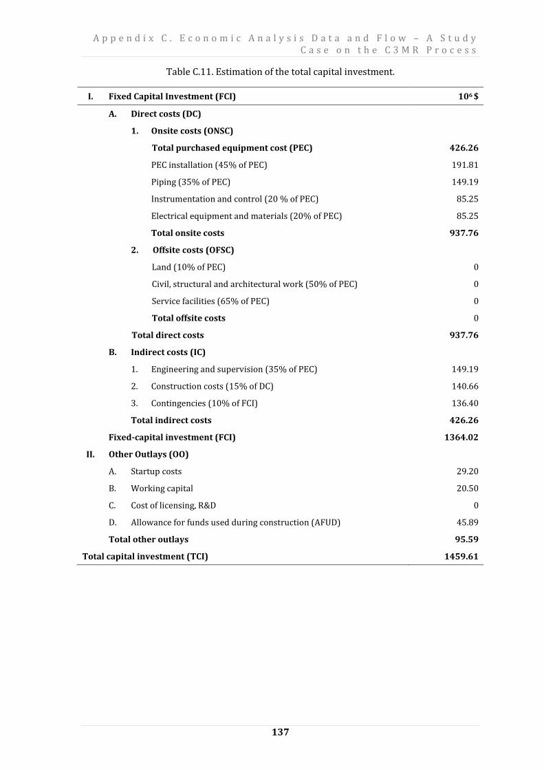
A p p e n d i x C . E c o n o m i c A n a l y s i s D a t a a n d F l o w – A S t u d y C a s e o n t h e C 3 M R P r o c e s s
137
Table C.11. Estimation of the total capital investment.
I. Fixed Capital Investment (FCI) 106 $
A. Direct costs (DC)
1. Onsite costs (ONSC)
Total purchased equipment cost (PEC) 426.26
PEC installation (45% of PEC) 191.81
Piping (35% of PEC) 149.19
Instrumentation and control (20 % of PEC) 85.25
Electrical equipment and materials (20% of PEC) 85.25
Total onsite costs 937.76
2. Offsite costs (OFSC)
Land (10% of PEC) 0
Civil, structural and architectural work (50% of PEC) 0
Service facilities (65% of PEC) 0
Total offsite costs 0
Total direct costs 937.76
B. Indirect costs (IC)
1. Engineering and supervision (35% of PEC) 149.19
2. Construction costs (15% of DC) 140.66
3. Contingencies (10% of FCI) 136.40
Total indirect costs 426.26
Fixed-capital investment (FCI) 1364.02
II. Other Outlays (OO)
A. Startup costs 29.20
B. Working capital 20.50
C. Cost of licensing, R&D 0
D. Allowance for funds used during construction (AFUD) 45.89
Total other outlays 95.59
Total capital investment (TCI) 1459.61

A p p e n d i x C . E c o n o m i c A n a l y s i s D a t a a n d F l o w – A S t u d y C a s e o n t h e C 3 M R P r o c e s s
138
C.2.2 Estimation of allowance for funds used during construction
(AFUDC)
The plant facilities investment (PFI) is provided in the equation (C.12). The land cost is
excluded from the economic analysis thus the PFI is equal to the plant fixed capital
investment. With an annual rate of 5 % to December 31, 2014, 40% of the plant facilities
investment should be escalated, and the rest of it (which accounts 60%) should be escalated
to December 31, 2015. This is according to the parameters assumed in the economic
analysis.
LandJan.1,2012Jan.1,2012 CostFCIPFI −= (C.12)
The allowance for funds used during construction for the liquefaction plant is calculated
separately and listed in Table C.12. It is based on the parameters assumed for the plant
financing fractions and required returns on capital. The total AFUDC calculated is
72.214*106 $ at the end of the year 2015. Consequently, the evaluations of the total non-
depreciable (TNI)7 in the equation (C.13) and depreciable capital investments (TDI) in
equation (C.14) for the liquefaction plant are carried out.
AFUDCEquityCommon++= WCCostTNI Land (C.13)
6
5Dec.31.201 10*497.56TNI =
Assessing the total depreciable capital investment as
TNITCITDI −= (C.14)
6
5Dec.31.201 10*115.1403TDI = $.
After the total depreciable investment (TDI) calculation, the modified accelerated cost
recovery system (MACRS) factors can be estimated for the tax life of the system which is 15
years. It is significant to note that, according to MACRS the depreciation is calculated for one
more extra years. Therefore, for a system that has the tax life of 15 years, the depreciation
should be calculated for 16 years (Table C.13) [62].
7 defined as the sum of the land cost, working capital and common equity of AFUDC.

A p p e n d i x C . E c o n o m i c A n a l y s i s D a t a a n d F l o w – A S t u d y C a s e o n t h e C 3 M R P r o c e s s
139
Table C.12. The calculated values for the allowance for funds used during construction (106 $).
Plant-Facilities Investment Common Equity Preferred Equity Debt
Construction
Year
Calendar
Year
In Jan.1,2012
Dollars
Amount of
Escalation
Escalated
Investment
Escalated
Investment
AFUDC
Escalated
Investment
AFUDC
Escalated
Investment
AFUDC
1 2014 545.609 55.925 601.533 210.537 31.581 90.230 10.557 300.767 30.077
2 2015 818.413 129.002 947.415 331.595 0.000 142.112 0.000 473.708 0.000
Subtotals 1364.021 184.927 1548.948 542.132 31.581 232.342 10.557 774.474 30.077
Total AFUDC 72.214
Total AFUDC in 2012 45.893

A p p e n d i x C . E c o n o m i c A n a l y s i s D a t a a n d F l o w – A S t u d y C a s e o n t h e C 3 M R P r o c e s s
140
Table C.13. Statutory percentages for use in the MACRS for a life period of 15 years, annual
tax depreciation and tax book at the end of each year for the LNG plant.
Year of Commercial Operation
Calendar
Year
MACRS Depreciation
Factor (%)
Annual Tax Depreciation
(106$)
End-Year Tax Book Value
(106$)
0 2015 - - 1403.115
1 2016 5.00 70.156 1332.960
2 2017 9.50 133.296 1199.664
3 2018 8.55 119.966 1079.697
4 2019 7.70 108.040 971.657
5 2020 6.93 97.236 874.421
6 2021 6.23 87.414 787.007
7 2022 5.90 82.784 704.224
8 2023 5.90 82.784 621.440
9 2024 5.91 82.924 538.516
10 2025 5.90 82.784 455.732
11 2026 5.91 82.924 372.808
12 2027 5.90 82.784 290.024
13 2028 5.91 82.924 207.100
14 2029 5.90 82.784 124.316
15 2030 5.91 82.924 41.392
16 2031 2.95 41.392 0.000
Totals 100.00 1403.115

A p p e n d i x C . E c o n o m i c A n a l y s i s D a t a a n d F l o w – A S t u d y C a s e o n t h e C 3 M R P r o c e s s
141
C.3 Estimation of Operating and Maintenance (O&M)
Costs
The operating and maintenance costs are defined as the total of the fixed and variable costs.
The compounds of the fixed O&M costs are operating labor, maintenance labor, maintenance
materials, overhead, administration and support, distribution and marketing and so on. For
the maintenance and operation of the plant, 30 labor positions are expected with an average
labor rate of 2.24 $ per hour assumed for Malaysia. The labor cost value is achieved for the
year 2009 and escalated to 2011. The average working hours for a labor position is
considered as 2080 hrs per annum, and the yearly direct labor cost is evaluated as
0.154*106 $. Based on this evaluation, the yearly fixed O&M costs and the yearly variable
O&M costs at full capacity are valued at 0.336*106 $ and 0.031*106 $, respectively.
Considering the capacity factor of the plant, these values are calculated as 0.286*106 $ and
0.026*106 $, respectively [107].
To calculate the corresponding costs for the first year of the operation, these fixed and
variable O&M costs are escalated at a nominal escalation rate of 5 % per year to the Jan.1,
2016.
$10*364.0)1(* 65 =+= nfixedJan.1,2011fixedJan.1,2016 iM&OM&O
$10*033.0)1(* 65 =+= nvariableJan.1,2011variableJan.1,2016 iM&OM&O
A p p e n d i x C . E c o n o m i c A n a l y s i s D a t a a n d F l o w – A S t u d y C a s e o n t h e C 3 M R P r o c e s s
142
C.4 Estimation of the Fuel Costs (FC)
Fuel costs are typically a part of operating and maintenance costs. Nevertheless, they are
determined independently in this analysis because of their importance for the thermal
systems. In LNG plants, the fuel of the system is normally the electricity supplied to the
propane and mixed refrigerant compressors. The unit electricity price in Malaysia is 25
Malaysian cents per kWh for the year 2011. The fuel price is then calculated as 98.162*106 $
in view of the working hours 7446 hrs in a year with 85 % of plant availability and the total
power consumption of the compressors as 156.22 MW. The calculated value is escalated to
the Jan.1, 2016 with an escalation rate of 6 % as [108].
65 10*364.131)1(* =+= nJan.1,2011Jan.1,2016 iFCFC $

A p p e n d i x C . E c o n o m i c A n a l y s i s D a t a a n d F l o w – A S t u d y C a s e o n t h e C 3 M R P r o c e s s
143
C.5 Estimation of Revenue Requirements
The annual total revenue requirement (TRR) of a thermal plant is defined as the income that
must be gained in a specified year. It should come from the trade of all the yields of the plant
to pay the system operating business for the expenses acquired in the same specified year.
This is also to ensure plant operation is economically sound. TRR is assessed as the total of
the eight yearly amounts: total capital recovery (TCR); minimum return on investment (ROI)
for common equity (ce), preferred stock (ps) and debt (d); income taxes (ITX); other taxes
and insurance (OTXI); fuel costs (FC); and operating and maintenance costs (O&M). Equation
(C.15) states such as follows [62]:
jjjjdj,psj,cej,jj M&OFCOTXIITXROIROIROITCRTRR +++++++= (C.15)
(9) (1) (2) (3) (4) (5) (6) (7) (8)
The year-by-year evaluation is executed to evaluate the levelized revenue requirement. It is
shown in Table C.14.
Meanwhile, the annuities and the cost levelization involved in the revenue requirements
estimates will refer to the following correlations ((C.16) to (C.17)) and ((C.18) to (C.19))
[62,83], respectively.
( )( )neffeff
n
eff
ii
iAP
+
−+=
1
11
(C.16)
( )( ) 11
1
−+
+==
n
eff
n
effeff
i
ii
P
ACRF
(C.17)
( )( ) CRF
k
kkFCCELFFCFC
FC
FCn
FC00L −
−×=×=
1
1
(C.18)
( )( ) CRF
k
kkOMCCELFOMCOMC
OMC
OMCn
OMC00L −
−×=×=
1
1
(C.19)
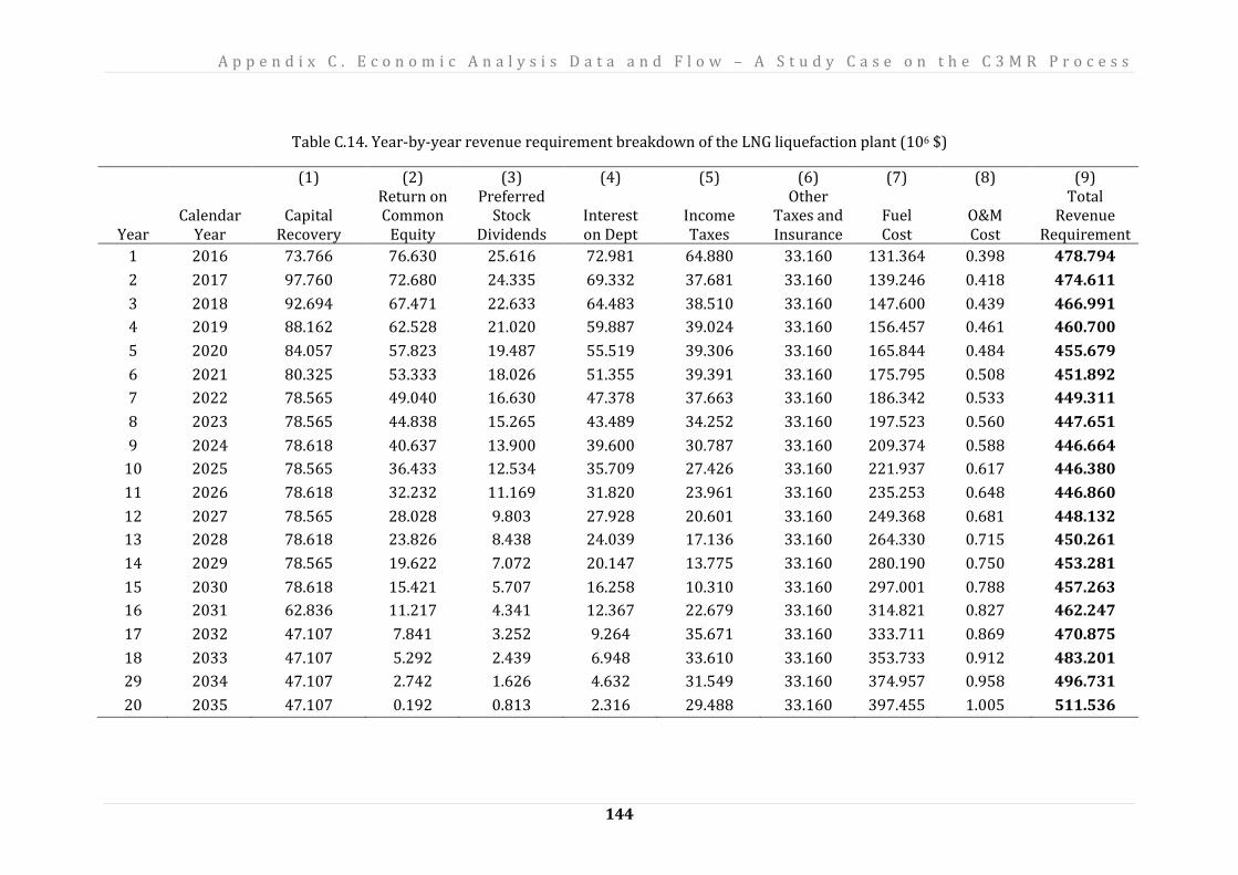
A p p e n d i x C . E c o n o m i c A n a l y s i s D a t a a n d F l o w – A S t u d y C a s e o n t h e C 3 M R P r o c e s s
144
Table C.14. Year-by-year revenue requirement breakdown of the LNG liquefaction plant (106 $)
Year
Calendar Year
(1)
Capital Recovery
(2) Return on Common
Equity
(3) Preferred
Stock Dividends
(4)
Interest on Dept
(5)
Income Taxes
(6) Other
Taxes and Insurance
(7)
Fuel Cost
(8)
O&M Cost
(9) Total
Revenue Requirement
1 2016 73.766 76.630 25.616 72.981 64.880 33.160 131.364 0.398 478.794
2 2017 97.760 72.680 24.335 69.332 37.681 33.160 139.246 0.418 474.611
3 2018 92.694 67.471 22.633 64.483 38.510 33.160 147.600 0.439 466.991
4 2019 88.162 62.528 21.020 59.887 39.024 33.160 156.457 0.461 460.700
5 2020 84.057 57.823 19.487 55.519 39.306 33.160 165.844 0.484 455.679
6 2021 80.325 53.333 18.026 51.355 39.391 33.160 175.795 0.508 451.892
7 2022 78.565 49.040 16.630 47.378 37.663 33.160 186.342 0.533 449.311
8 2023 78.565 44.838 15.265 43.489 34.252 33.160 197.523 0.560 447.651
9 2024 78.618 40.637 13.900 39.600 30.787 33.160 209.374 0.588 446.664
10 2025 78.565 36.433 12.534 35.709 27.426 33.160 221.937 0.617 446.380
11 2026 78.618 32.232 11.169 31.820 23.961 33.160 235.253 0.648 446.860
12 2027 78.565 28.028 9.803 27.928 20.601 33.160 249.368 0.681 448.132
13 2028 78.618 23.826 8.438 24.039 17.136 33.160 264.330 0.715 450.261
14 2029 78.565 19.622 7.072 20.147 13.775 33.160 280.190 0.750 453.281
15 2030 78.618 15.421 5.707 16.258 10.310 33.160 297.001 0.788 457.263
16 2031 62.836 11.217 4.341 12.367 22.679 33.160 314.821 0.827 462.247
17 2032 47.107 7.841 3.252 9.264 35.671 33.160 333.711 0.869 470.875
18 2033 47.107 5.292 2.439 6.948 33.610 33.160 353.733 0.912 483.201
29 2034 47.107 2.742 1.626 4.632 31.549 33.160 374.957 0.958 496.731
20 2035 47.107 0.192 0.813 2.316 29.488 33.160 397.455 1.005 511.536
A p p e n d i x C . E c o n o m i c A n a l y s i s D a t a a n d F l o w – A S t u d y C a s e o n t h e C 3 M R P r o c e s s
145
C.5.1 Total capital recovery
The total net investment of the system must be recovered during the assumed economic life
of the plant. Calculations of the total capital recovery of the natural gas liquefaction plant are
conducted by year by year analysis and illustrated in Table C.15. According to this table the
column D (total capital recovery) is previously calculated and illustrated in total revenue
requirement in Table C.14. The book life (BL) and the total depreciable investment (TDI) are
used to calculate the annual book depreciation (BD), shown in the column A of Table C.15 by
applying the straight-line method described as [62].
BL
TDIBD j = , j =1, ..., BL (C.20)
where the index j represents the j-th year of the book life. The deferred income taxes (DITX)
for the j-th year of tax life (TL) is illustrated in column B of Table C.15 which are coming
from the difference between the annual tax depreciation (TXD), which is expressed by the
equation (C.21) and using the MACRS method. The annual book depreciation (BD) is
calculated by the equation (C.22), where the term t denotes the average combined income
tax rate in Table C.1 [62].
jMACRS,j f*TDITDX = , j = 1, …, TL+1 (C.21)
( ) t*BDTXDDITX jjj −= , j = 1, …, TL+1 (C.22)
BL
CEAFRCEAF j = , j =1, ..., BL
(C.23)
The common equity allowance for funds used during the construction (CEAF) that is not
considered in the net depreciable investment is recovered by applying a constant annual
amount (RCEAF). It is illustrated in the column C of the Table C.15 and calculated by the
equation (C.23), where CEAF represents the common equity AFUDC at the end of the design
and construction period [62].
The total capital recovery (TCR) for the j-th year of book life is the sum of the book
depreciation, deferred income taxes and recovery of the common equity AFUDC as shown as
jjjj RCEAFDITXBDTCR ++= , j = 1, …, BL (C.24)

A p p e n d i x C . E c o n o m i c A n a l y s i s D a t a a n d F l o w – A S t u d y C a s e o n t h e C 3 M R P r o c e s s
146
Table C.15. Year by year capital recovery schedule for the LNG plant. (106 $)
Year of
Commercial Operation
Calendar
Year
(A) Annual Book Depreciation
(B) Deferred
Income Taxes
(C) Recovery of
Common Equity AFUDC
(D) Total
Capital Recovery
1 2016 70.156 0.000 3.611 73.766
2 2017 70.156 23.993 3.611 97.760
3 2018 70.156 18.928 3.611 92.694 4 2019 70.156 14.396 3.611 88.162 5 2020 70.156 10.290 3.611 84.057 6 2021 70.156 6.558 3.611 80.325
7 2022 70.156 4.799 3.611 78.565
8 2023 70.156 4.799 3.611 78.565
9 2024 70.156 4.852 3.611 78.618
10 2025 70.156 4.799 3.611 78.565 11 2026 70.156 4.852 3.611 78.618 12 2027 70.156 4.799 3.611 78.565
13 2028 70.156 4.852 3.611 78.618
14 2029 70.156 4.799 3.611 78.565
15 2030 70.156 4.852 3.611 78.618
16 2031 70.156 -10.930 3.611 62.836 17 2032 70.156 -26.659 3.611 47.107 18 2033 70.156 -26.659 3.611 47.107
19 2034 70.156 -26.659 3.611 47.107
20 2035 70.156 -26.659 3.611 47.107
Subtotal 1403.115 0 72.214 1475.329
Total Investment 1459.612
C.5.2 Returns on equity and debt
The distribution of capital recovery among debt, preferred stock and common equity year-
by-year for the LNG plant is shown in Table C.16. This table is applied to calculate the
balance representing the basis for determining the returns on equity and the debt interest.
It is listed in Table C.14, columns 2-4, at the beginning of each year for each type of
financing. The total investment is distributed considering the financing fractions (see Table
C.1). Determination of the balances at the beginning of the first year (BBY1,x) for the xth type
of financing is expressed as
x1,x f*TNIBBY = , x = d, ps, ce (C.25)
The adjustment columns in the Table C.16 for different fractions of financing are analyzed
using the following equations. Additionally, the adjustment column for common equity also
includes the recovery of common equity allowance for funds used during construction.

A p p e n d i x C . E c o n o m i c A n a l y s i s D a t a a n d F l o w – A S t u d y C a s e o n t h e C 3 M R P r o c e s s
147
djdj, fDITXADJ = , j = 1, …, BL (C.26)
psjpsj, fDITXADJ = , j = 1, …, BL (C.27)
jcejcej, RCEAFfDITXADJ += , j = 1, …, BL (C.28)
The columns representing the book depreciation in Table C.16 are evaluated for each type of
financing by applying the straight-line depreciation
BL
ADJBBY
BD
BL
1kk,x,x
j,x
∑−= =
1
, j =1, …, BL, x = d, ps, ce
(C.29)
The balance at the beginning of the j th year for each type of financing is assessed as
( )j,xj,x1,xjj,x ADJBDBBYBBY +−= − , j = 2, …, BL, x = d, ps, ce (C.30)
The return on investment (ROI) for the year j is shown as
xj,xj,x iBBYROI = , j = 1, …, BL , x = d, ps, ce (C.31)
where ix accounts for the annual rate of return for the xth investment.
C.5.3 Taxes and insurance
Taxes and insurance are valued in the columns 5 and 6 in the Table C.14. The income taxes
(ITXj) which are to be paid during the j th year are analyzed through the equation (C.32)
( ) jjpsj,cej,j DITXRCEAFROIROIt
tITX −++
−=
1
(C.32)
where the term t is the total income tax rate, listed in Table C.1. The yearly sum of the other
taxes (property taxes) and insurance costs (OTXI) may be evaluated as a constant
percentage of the escalated plant facilities investment (PFI) as
OTXIj f*PFIOTXI = , j = 1, …, BL (C.33)
where the value of the factor fOTXI is assumed to be 2 %, listed in Table C.1 (entries 5b and
5c).
C.5.4 Fuel, operating and maintenance costs
The total fuel costs and O&M costs for the LNG plant for the first year of the operation are
considered in the subchapters C.3 and C.4 as 0.397*106 $ /year and 131.364*106 $/year,
respectively.

A p p e n d i x C . E c o n o m i c A n a l y s i s D a t a a n d F l o w – A S t u d y C a s e o n t h e C 3 M R P r o c e s s
148
C.5.5 Total revenue requirement (TRR)
Total revenue requirement for the LNG plant is evaluated for each year separately with the
aid of the equation (C.15) and is provided in the last column of the Table C.14.

A p p e n d i x C . E c o n o m i c A n a l y s i s D a t a a n d F l o w – A S t u d y C a s e o n t h e C 3 M R P r o c e s s
149
Table C.16. Distribution of capital recovery for the LNG plant (106 $).
Debt
Preferred Stock
Common Equity
Year
Calendar
Year
Balance Beginning
of Year
Book
Depreciation
Adjustment
Balance
Beginning of Year
Book
Depreciation
Adjustment
Balance
Beginning of Year
Book
Depreciation
Adjustment
Total Capital
Recovery
1 2016 729.806 36.490 0.000 218.942 10.947 0.000 510.864 22.718 3.611 73.766
2 2017 693.316 36.490 11.997 207.995 10.947 3.599 484.535 22.718 12.008 97.760
3 2018 644.829 36.490 9.464 193.449 10.947 2.839 449.808 22.718 10.236 92.694
4 2019 598.874 36.490 7.198 179.662 10.947 2.159 416.855 22.718 8.649 88.162
5 2020 555.186 36.490 5.145 166.556 10.947 1.544 385.487 22.718 7.212 84.057
6 2021 513.551 36.490 3.279 154.065 10.947 0.984 355.556 22.718 5.906 80.325
7 2022 473.781 36.490 2.399 142.134 10.947 0.720 326.932 22.718 5.290 78.565
8 2023 434.892 36.490 2.399 130.468 10.947 0.720 298.923 22.718 5.290 78.565
9 2024 396.002 36.490 2.426 118.801 10.947 0.728 270.915 22.718 5.309 78.618
10 2025 357.086 36.490 2.399 107.126 10.947 0.720 242.887 22.718 5.290 78.565
11 2026 318.196 36.490 2.426 95.459 10.947 0.728 214.879 22.718 5.309 78.618
12 2027 279.280 36.490 2.399 83.784 10.947 0.720 186.851 22.718 5.290 78.565
13 2028 240.390 36.490 2.426 72.117 10.947 0.728 158.843 22.718 5.309 78.618
14 2029 201.474 36.490 2.399 60.442 10.947 0.720 130.816 22.718 5.290 78.565
15 2030 162.584 36.490 2.426 48.775 10.947 0.728 102.807 22.718 5.309 78.618
16 2031 123.668 36.490 -5.465 37.100 10.947 -1.640 74.780 22.718 -0.215 62.836
17 2032 92.643 36.490 -13.330 27.793 10.947 -3.999 52.276 22.718 -5.720 47.107
18 2033 69.482 36.490 -13.330 20.845 10.947 -3.999 35.278 22.718 -5.720 47.107
19 2034 46.321 36.490 -13.330 13.896 10.947 -3.999 18.279 22.718 -5.720 47.107
20 2035 23.161 36.490 -13.330 6.948 10.947 -3.999 1.281 22.718 -5.720 47.107
21 2035 0 36.490 0 0.000 10.947 0 -15.717 22.718 0 70.156
Totals 729.806 0 218.942 0 454.367 72.214 1475.329

A p p e n d i x C . E c o n o m i c A n a l y s i s D a t a a n d F l o w – A S t u d y C a s e o n t h e C 3 M R P r o c e s s
150
C.5.6 Levelized Costs and the Cost of the Main Product
The evaluation of the annual values of carrying charges (CC), fuel costs (FC) and O&M
expenses of a thermal system is necessary for the evaluation of the design modifications and
cost effectiveness. These cost components are expected to vary considerably over the entire
economic life of the production facilities. Carrying costs show a decreasing trend where the
fuel and O&M charges tend to increase with increasing years of operation. Therefore, it is
recommended to use levelized annual values for cost components in terms of design
modifications. The levelized value of the annual total revenue requirement is assessed by
taking the summation of the present values of the 20 annual values in Table C.14. These
values are then converted to equivalent annuities with the help of the equation (C.16). The
average cost of money (ieff) of 12 % is assumed as the discount rate during the evaluations.
The levelized fuel costs (FCL) are considered with the aid of the equations (C.17) and
(C.18) as
946.012.01
06.01=
++
=Fk
134.01)12.01(
)12.01(12.020
20
=−+
+=CRF
6206
10*145.190)946.01(
)134.0)(946.01(
06.1
10*364.131=
−−
×=LFC $.
Equally, the levelized annual operating and maintenance costs (OMCL) are projected using
the equations (C.17) and (C.19):
9375.012.01
05.01=
++
=OMk
6206
10*538.0)9375.01(
)134.0)(9375.01(9375.0
05.1
10*398.0=
−−
×=LOMC .
The levelized annual total revenue requirement is calculated as the sum of the
present values of 20 annual values given in year by year analysis in Table C.14. It is the
converted to an equivalent annuity with the aid of the equation (C.17).
∑==
−−
20
1nyearbyyearP TRRTRR
$10*595.46110*861.3447*134.0 66 === PL TRR*CRFTRR .

A p p e n d i x C . E c o n o m i c A n a l y s i s D a t a a n d F l o w – A S t u d y C a s e o n t h e C 3 M R P r o c e s s
151
The levelized annual carrying charges (CCL) can be estimated then as
$10*912.270 6=−−= LLLL OMCFCTRRCC
The ratio between the annual total revenue requirement (TRR) and the product
quantity (MPQ) calculates the unit cost of the product (MPUC):
MPQ
TRRMPUC L=
(C.34)
The primary product of the liquefaction plant is the liquefied natural gas with a mass
flow rate of 158.4 kg/s. The yearly quantity of the product is calculated seeing the plant
capacity of 85% as follow
610*246.41744636004.158 ==kg
Ton
yr
h
h
s
s
kgMPQ Ton/yr.
The levelized unit cost of the liquefied natural gas is then considered using the equation
(C.34):
kgTon /$11.0/$71.108Ton10*246.4
$10*595.461
MPQ
TRRMPUC
6
6L ====

A p p e n d i x C . E c o n o m i c A n a l y s i s D a t a a n d F l o w – A S t u d y C a s e o n t h e C 3 M R P r o c e s s
152
Table C.17. LNG plant data set [98].
LNG Plant
Country Startup
Year Technology
Capacity (mtpa)
Capital Unit Costs
($ bn/mtpa)
Marsa El Brega Libya 1970 APCI 2.6 0.163
Lumut Brunei 1972 APCI 5.3 0.253
Arun, Phase 1 Indonesia 1978 APCI 4.2 0.532
Adgas, Das Island Abu Dhabi 1977 APCI 3.0 0.414
Bonny Island, T1+2 Nigeria 1999 APCI 5.9 0.421
Bonny Island T3 Nigeria 2002 APCI 2.9 0.289
MLNG I, Bintulu Malaysia 1984 APCI 6.0 0.495
MLNG II (Dua) Malaysia 1995 APCI 5.2 0.403
MLNG III (TIGA) Malaysia 2003 APCI 7.6 0.211
Damietta Egypt 2005 APCI 5.0 0.208
Bonny Island, T4+5 Nigeria 2005 APCI 8.0 0.217
Qalhat, T3 Oman 2006 APCI 3.30 0.189

A p p e n d i x C . E c o n o m i c A n a l y s i s D a t a a n d F l o w – A S t u d y C a s e o n t h e C 3 M R P r o c e s s
153
Table C.18. Economic data for the selected LNG plants [98].
LNG Plant Country Initial
Start-up Capacity/ train
(MTA) Capital Unit Costs (2013 $ bn/MTA)
One train
Adgas, Das Island Abu Dhabi 1994 2.60 0.635
Bontang Indonesia 1998 3.00 0.605
Damietta Egypt 2005 5.00 0.293
Qalhat Oman 2006 3.30 0.267
Two trains
Rasgas Qatar 1999 2.60 0.443
Qalhat Oman 1999 3.00 0.388
MLNG Malaysia 2003 3.80 0.298
Bonny Island Nigeria 2005 4.00 0.306
Tangguh Indonesia 2007 3.50 0.282
Three trains
Burrup Northwest
Australia 1989 2.00 0.638
MLNG Malaysia 1995 2.60 0.569
Qatargas Qatar 1998 2.50 0.427
Bonny Island Nigeria 1999 3.20 0.594
Bonny Island Nigeria 2002 3.70 0.408
Seven trains
Bontang Indonesia 1999 2.60 0.368