General rights Copyright and moral rights for the publications made accessible in the public portal are retained by the authors and/or other copyright owners and it is a condition of accessing publications that users recognise and abide by the legal requirements associated with these rights.

Users may download and print one copy of any publication from the public portal for the purpose of private study or research.

You may not further distribute the material or use it for any profit-making activity or commercial gain

You may freely distribute the URL identifying the publication in the public portal If you believe that this document breaches copyright please contact us providing details, and we will remove access to the work immediately and investigate your claim.

Downloaded from orbit.dtu.dk on: Jan 11, 2020

Thermocline thermal storage systems for concentrated solar power plants: One-dimensional numerical model and comparative analysis

Modi, Anish; Perez-Segarra, Carlos David

Published in:Solar Energy

Link to article, DOI:10.1016/j.solener.2013.11.033

Publication date:2014

Link back to DTU Orbit

Citation (APA):Modi, A., & Perez-Segarra, C. D. (2014). Thermocline thermal storage systems for concentrated solar powerplants: One-dimensional numerical model and comparative analysis. Solar Energy, 100, 84-93.https://doi.org/10.1016/j.solener.2013.11.033

1

Thermocline thermal storage systems for concentrated solar power plants: One-dimensional numerical model and comparative analysis

Anish Modi a, 1, Carlos David Pérez-Segarrab a Department of Mechanical Engineering, Technical University of Denmark (DTU), Nils Koppels Allé, Bldg. 403, Kgs. Lyngby – 2800, Denmark

bCentre Tecnològic de Transferència de Calor (CTTC), Universitat Politècnica de Catalunya (UPC), ETSEIAT, C/Colom 11, Terrassa – 08222, Spain

Abstract Concentrated solar power plants have attracted increasing interest from researchers and governments all over the world in recent years. An important part of these plants is the storage system which improves dispatchability and makes the plant more reliable. In this paper, a one-dimensional transient mathematical model for a single-tank thermocline thermal energy storage system is presented. The model used temperature dependent correlations to obtain the thermophysical properties for the heat transfer fluid and considered heat loss through the tank wall. The effect of variation in important system parameters like the type of heat transfer fluid, the storage temperature difference and the cycle cut-off criterion on system performance was investigated. The results suggest that two important aspects for assessing the performance of the system are the cyclic behaviour of the system and the time required to attain equilibrium conditions. These aspects directly influence the discharge capacity and discharge power of the storage system, and therefore play an essential role in understanding the start-up characteristics of the system and provide an insight regarding the availability of storage when designing the power cycle for concentrated solar power applications. It was also observed that the cycle durations and the time required to attain cyclic conditions are highly sensitive to not only the storage temperature difference, but also the cut-off temperature difference.

Keywords Concentrated solar power; thermocline storage; numerical model; cyclic behaviour

Highlights • One-dimensional mathematical model for high temperature thermocline thermal storage tank • Temperature dependent thermophysical properties of the HTF • Heat loss from tank walls considered using overall heat loss coefficient • Cyclic behaviour indicates independence from initial conditions • Storage temperature difference, cut-off criteria and type of HTF have high impact on cycle durations

1 Introduction In recent times, concentrated solar power (CSP) plants have increasingly been regarded as viable candidates for large-scale electricity generation (Greenpeace International et al. 2009). CSP technologies have matured considerably over the last few years thanks to innovations in the collectors, thermal energy storage (TES) systems and novel approaches like concentrated solar photovoltaics and solar thermoelectrics (Fernández-García et al. 2010; Barlev et al. 2011). With suitable support, it has been estimated that CSP could satisfy 11.3% of global electricity demand by the year 2050 – out of which 9.6% would be from solar power and the rest from back-up fuels (International Energy Agency 2010). In theory, a CSP plant consists of three key sections: the solar field, the storage system and the power block. Of these, the capacity of the storage system determines the proportion of time for which power is available. An affordable energy storage method is thus a crucial element in a successful year-round operation of a solar thermal power plant (Barlev et al. 2011). However, it is also one of the less developed parts and only a few CSP plants in the world have tested high temperature TES systems (between 120 °C and 600 °C) (Gil et al. 2010). TES systems are usually classified into three types: sensible, latent and thermochemical (Dincer & Dost 1996). The current study focuses on the thermal and cyclic behaviour of a high temperature single-tank sensible thermocline storage tank. The thermocline thermal energy storage (TTES) system has the potential to reduce the overall cost of the plant since most of the expensive storage fluid can be replaced by low cost filler material (Gil et al. 2010; Brosseau et al. 2005). This potential resulted in an increased interest in evaluating such systems through modelling and simulations. Van Lew et al. (Van Lew et al. 2009) investigated the interactions between the heat transfer fluid (HTF) and the filler material using a dimensionless form of the Schumann model

1 Corresponding author: anmod@mek.dtu.dk; +45-45251910

2

(Schumann 1929). The same research group also presented generalized charts of energy storage effectiveness for thermocline tank design, and proposed calibration as an effective tool to size the tanks (Van Lew et al. 2009; Karaki et al. 2010; Van Lew et al. 2011; Li et al. 2011; Valmiki et al. 2012). Tesfay and Venkatesan (Tesfay & Venkatesan 2013) presented a one-dimensional model using Schumann equations simulating the model in C programming language. Bayón and Rojas (Bayón & Rojas 2013) presented a single phase one-dimensional model highlighting the importance of certain design parameters such as size of the tank, thermal power and charge/discharge time while designing a tank in practice, and provided guideline plots to be used in the design process of thermocline prototypes. A detailed two-temperature two-dimensional model was presented by Yang and Garimella (Yang & Garimella 2010b) to study the discharge process of the thermocline system with molten salt and filler material. The same group also conducted a thermomechanical analysis of the tank walls to study the thermal ratcheting phenomenon involved with the tank walls (Yang & Garimella 2010b; Yang & Garimella 2010a; Flueckiger et al. 2011; Yang & Garimella 2013; Flueckiger et al. 2012). Fluekiger et al. (Flueckiger et al. 2014) showed that by employing a 6 h storage capacity using a TTES system for a 100 MW central receiver CSP plant working with a simple Rankine cycle, it is possible to increase the annual plant capacity factor from 27.3% to 53.1% and the annual solar-to-electricity efficiency of the plant from 7.6% to 14.7%. The authors assumed perfect insulation and one-dimensional behaviour of the tank for the annual performance analysis. Xu et al. (Xu et al. 2012b) presented a two-dimensional, two-phase model for heat transfer and fluid dynamics within the thermocline storage system. The authors used the model to evaluate different correlations for the interstitial heat transfer coefficient, effective thermal conductivity and the effect of the thermal conductivity of solid fillers. The effect of insulation on thermal behaviour was also presented. The authors concluded that a uniform cross-sectional temperature can be attained with two insulation layers and that the thermocline region can cover more than 1/3rd of the tank height at its maximum thickness for a tank height of 14 m. The same authors also published results from the effects of fluid inlet velocity, inlet temperature, porosity, tank height and solid particle properties on the thermal performance of a TTES system (Xu et al. 2012b; Xu et al. 2012a; Xu et al. 2013). The published one- and two-dimensional models examined the effect of varying system parameters such as porosity, filler material diameter, tank dimensions etc. on overall performance of the TTES system. The one-dimensional models by Van Lew et al. (Van Lew et al. 2009) and Tesfay and Venkatesan (Tesfay & Venkatesan 2013) assume constant thermophysical properties for the HTF and no heat loss to the environment. The model by Bayón and Rojas (Bayón & Rojas 2013) considers the thermal losses to the environment, but it is a single-phase model assuming thermal equilibrium between the HTF and the filler bed. The assumption of constant thermophysical properties, local thermal equilibrium between the HTF and the filler bed or no heat loss to the environment makes these models overly simplified. For example, the operation of a TTES system is in fact due to the buoyancy effect caused by density difference between the hot and the cold sections of the tank, and that the significant difference between the thermophysical properties of the HTF and the filler material calls for a two-temperature model accounting for local thermal non-equilibrium. The two-dimensional models (Yang & Garimella 2010b; Xu et al. 2012b) on the other hand are detailed models, but at the same time are computationally intensive. Most of the above studies were focussed on evaluating the tank performance with a particular type of HTF and with adiabatic conditions. To the authors’ knowledge, there have been no studies regarding the comparison of using different HTFs in the TTES systems and the evaluation of the TTES system performance based on the storage temperature difference and the cut-off temperature difference, and their effect on the cycle durations. The current study attempts to fill these gaps by presenting a numerical model of the TTES system considering local thermal non-equilibrium between the HTF and the filler bed and thermal losses to the ambient; using temperature dependent thermophysical properties for the HTF; comparing the performance of the three most commonly considered HTF for CSP applications; and comparing the performance of the TTES system depending on the storage temperature difference and the cut-off temperature difference when using Solar Salt (a 60%-40% mixture of sodium nitrate and potassium nitrate respectively by wt.) as the HTF. The objective of this paper is thus to present a simplified one-dimensional model and its validation using the experimental data by Pacheco et al. (Pacheco et al. 2002) so as to have a computationally non-intensive model which can be integrated with the design of the power cycle for CSP applications for a sufficiently accurate evaluation of the storage system on an overall level. In addition, the current model demonstrates the importance of considering the cyclic behaviour of the storage system and the time required to attain stability in operating conditions which directly influences the response time of the storage system, its discharge rate and the storage capacity. Appropriate boundary conditions were applied to bring the analysis closer to the real operation of a CSP plant. These included assuming a storage hot temperature (Th in Figure 1) of 390 °C (in the range commonly used for parabolic trough CSP plants) and 560 °C (in the range commonly used for central receiver CSP plants). The effect of using different HTF, the temperature range for the operation of the storage system and the cut-off temperature difference on the duration of the charge and the discharge cycles was also studied. The results from this analysis would be helpful in designing or optimising the power cycle for CSP plants with regards to the availability and the capacity of the storage system. The study consisted of two parts: mathematical formulation of the heat transfer process including verification and validation methodologies for a reference case; and a comparative analysis using a hypothetical tank of larger dimensions based on the choice of the HTF, the storage hot temperature and the cut-off temperature difference. Section 2 presents the assumptions, the

3

numerical model, the solution algorithm and the validation procedure for the study. Section 3 presents the results from the model validation and the comparative analysis, while section 4 discusses the results from the comparative analysis. Finally, section 5 concludes the paper.

2 Methodology The reference case for modelling was considered to be the same tank as used by Pacheco et al. (Pacheco et al. 2002) so that the model could be validated against their experimental observations. The main assumptions for the modelling process were:

• The system parameters were assumed to change only in the axial direction reducing the model to a one-dimensional form along the tank axis. The storage tank was modelled as a cylindrical tank with cold fluid entering at the bottom of the tank and the hot fluid leaving from the top during the discharge cycle. The flow direction reverses during the charge cycle. Figure 1 shows the tank during a discharge cycle with the side walls and a division into ‘N’ control volumes (CVs) on the left; a typical CV with node notations is shown on the right. The nodes for the fluid were at the boundaries of the CV whereas the nodes for the filler bed were at the centre of the CV. This was so as to be able to apply the boundary conditions during a charge or discharge cycle with respect to the fluid, i.e., the cold fluid entering the tank during discharging was assumed to have a constant temperature Tc during the entire cycle. Similarly, the hot fluid entering the tank during charging was assumed to have a constant temperature Th during the entire cycle. Thus, there would be ‘N’ nodes for the filler bed and ‘N+1’ nodes for the HTF.

Figure 1: Tank (left) and control volume (right) representation during a typical discharge cycle

• The filler bed was assumed to be isotropic and homogeneous. Conduction in the filler bed was neglected as the filler material was assumed to be spherical and so the elements have only point contacts. The diameter of the spherical elements was small enough to assume constant temperature inside the spheres. Conduction in the HTF was also neglected.

• The thermophysical property relations for the reference case HTF (Solar Salt) for a temperature range of 300 °C to 600 °C are given in Table 1 (Zavoico 2001). For simplification, it was assumed that the same relations would hold true for ±10% of the mentioned temperature range.

Table 1: Correlations for thermophysical properties of Solar Salt (Zavoico 2001), T (°C)

Density kg/m3 2090 – 0.636 T Specific heat capacity J/kg-K 1443 + 0.172 T Absolute viscosity kg/m-s 2.2714·10-4 – 1.20·10-4 T + 2.281·10-7 T2 – 1.474·10-10 T3 Thermal conductivity W/m-K 0.443 + 1.9·10-4 T

The properties for the reference case filler material (quartzite rock/filter sand mixture) were assumed constant and taken to be: density = 2500 kg/m3; specific heat capacity = 830 J/kg-K; and thermal conductivity = 5.69 W/m-K. (Yang & Garimella 2010b; Xu et al. 2012a)

• The heat loss through the tank wall was represented using an overall heat transfer coefficient (Uloss) for the tank wall. It was assumed that only HTF was in contact with the tank on the inside. This is a reasonable assumption since the main mode of heat transfer is through convection from the HTF. The area of the tank touched by the HTF was used to calculate the heat transfer area per unit volume (aloss) in the energy balance equations. Losses from the top and bottom parts of

N

:

:

:

:

i

:

:

:

1

Tc

Th

H

D

Wall

Wall

Node ‘i’ for Tf

Node ‘i+1’ for Tf

Control VolumeBoundary

Node ‘i’ for Tb Δz

4

tank were neglected as the temperature profiles at the top and the bottom showed no visible shifts caused by thermal losses in these regions (Flueckiger et al. 2012). Since it is stated in the publication by Pacheco et al. (Pacheco et al. 2002) that the experimental set-up had electric heat-trace cables wrapped around the tank with good insulation to prevent heat losses, a relatively low value of Uloss (5 W/m2-K ) was assumed for the simulations. The ambient temperature (Text) was assumed to be constant at 25 °C.

• The HTF was assumed to have a uniform distribution at the entry and exit points. Not using the flow distributors at inlet and exit is thermally equivalent to using them as per Yang and Garimella (Yang & Garimella 2010b). In the current study, which is primarily a thermal analysis, the distributors were therefore not considered as a part of the system.

• An important aspect of this analysis was the cyclic behaviour of the storage system, and the time required to attain it. For this, a cut-off criterion was set to be a temperature difference of 20 °C from the normal operating condition, i.e., during a discharge cycle, the cycle was cut off as soon as the outlet temperature reached a value 20 °C below the storage hot temperature (Th); whereas during a charge cycle, the cycle was cut off as soon as the outlet temperature reached a value 20 °C above the system cold temperature (Tc). This value is dependent on the application of interest and for CSP plants, and a value of 20 °C was considered useful in generation of superheated steam (Xu et al. 2012b).

The reference case specifications are given in Table 2.

Table 2: Parameters for the reference case model

Parameter Symbol Value

HTF - Solar Salt

Filler bed - Quartzite rock + sand filler

Tank height H 6.1 m

Tank diameter D 3 m

Filler bed porosity ε 0.22

Diameter of quartzite rock Dp 0.01905 m

HTF inlet flow velocity (Darcy) w 4.186 x 10-4 m/s

Hot temperature of the storage system Th 390 °C

Cold temperature of the storage system Tc 290 °C

Overall heat loss coefficient for tank walls Uloss 5 W/m2-K

Ambient temperature Text 25 °C

Cut-off temperature at outlet for charge cycle - 310 °C

Cut-off temperature at outlet for discharge cycle - 370 °C

2.1 Governing equations The following equations were used to analyse the system (subscript f for the HTF and b for the filler bed). The equations were solved iteratively for all the CVs and for all time steps.

• Continuity equation for the HTF

( ) ( ) 0f f wt zερ ρ

∂ ∂+ =

∂ ∂ (1)

• Energy balance for the filler bed

( ) ( )1 bb b f b

TC h T T

t νε ρ∂

− = −∂

(2)

• Energy balance for the HTF

( ) ( )f f

b f loss loss f extf f f fT T

h T T U a T Tt z

C C w νερ ρ∂ ∂

+ = − − −∂ ∂

(3)

• The volumetric heat transfer coefficient hv (W/m3-K) was calculated using the following correlation as mentioned by Xu et al. (Xu et al. 2012a), where the ReP is the local Reynolds number based on Dp, and Pr is the local Prandtl number for the HTF.

( ) 0.6 1/3

2

6 1 2 1.1Re PrP

p

fv

k

Dh

ε− + = (4)

5

2.2 Solution algorithm and model validation With reference to Figure 1: for the charge cycle, the fluid flow was from node ‘i+1’ towards node ‘i', whereas for the discharge cycle, the flow was in the opposite direction, i.e., from node ‘i' to node ‘i+1’. Thus, during the charge cycle, the unknown variables were calculated at the fluid and the bed node ‘i' with known quantities at the fluid node ‘i+1’. Similarly, for the discharge cycle, the calculations were made for the unknown quantities at the fluid node ‘i+1’ and the bed node ‘i’ with known quantities at the fluid node ’i’. Finite volume technique was used for discretization of the governing equations with the upwind scheme for convective terms and the fully implicit scheme for time discretization. The code was verified for grid size and time step independence. A convergence criterion of 10-8 was used, i.e., any iteration was concluded when the residual was below or equal to 10-8. The solution algorithm is described below:

• The conditions at time t = 0 for the temperature profile inside the tank were given at the beginning to be used as an input to the model. The number of CVs (= N), porosity and other parameters such as the tank dimensions, filler bed thermophysical properties, flow velocity and cut-off criteria were also used as input data.

• The charge cycle was then initiated from the top of the tank with the inlet node (node ‘N+1’) temperature put equal to the storage hot temperature Th (390 °C for the reference case) as the boundary condition. At the end of the charge cycle, the discharge cycle was initiated from the bottom of the tank with the inlet node (node ‘1’) temperature put equal to the storage cold temperature Tc (290 °C for the reference case) as the boundary condition. The temperature distribution for the HTF and the filler bed at the beginning of the discharge cycle was the same as that at the end of its corresponding charge cycle. The idle time between the charge and the discharge cycles was not considered in this study as with adequate insulation, it would take as much as 100 h of standby time to observe a change in the temperature profile of the storage system (Xu et al. 2012a). This duration is much more than the idle time to be experienced by the storage system during the daily operation of the plant. The same procedure, as used for the charge cycle simulation, was followed to calculate the temperature profile of the HTF and the filler bed for the discharge cycle. Continuous charge and discharge cycles were simulated as loops to assess the cyclic behaviour of the system.

2.3 Comparative analysis considering a modified reference case The performance of a modified reference case was evaluated by studying the effects of variation in some important system parameters. In the modified reference case, the tank was assumed to have an internal diameter of 8 m and a height of 14 m. In view of the change in the tank height, a grid independence test was again performed and 4000 CVs were chosen for the comparative analysis. These are the only differences from the reference case (Table 2) for the purpose of comparative analysis. Comparisons based on the following parameters were made:

• HTF: The performance of the modified reference case was compared when using Solar Salt, HITEC or Therminol 66 as the HTF. The correlations for the thermophysical properties of HITEC molten salt (Yang & Garimella 2010b) and Therminol 66 (SOLUTIA 2013) are given in the Appendix.

• Storage hot temperature (Th): The performance of the modified reference case was analysed using Solar Salt as the HTF based on the storage temperature difference (i.e. the difference between the hot and the cold temperatures of the storage system) by varying the storage hot temperature. Two cases were compared: with Th = 390 °C and Th = 560 °C. The cut-off temperature at the outlet during a discharge cycle would therefore be 370 °C and 540 °C respectively. In both the cases, the storage cold temperature of the system was 290 °C, and therefore the cut-off temperature during a charge cycle for both the cases would be 310 °C.

• Cut-off temperature difference: The performance of the modified reference case was analysed using Solar Salt as the HTF with respect to change in the cut-off temperature difference from 20 °C to either 10 °C or 30 °C. Although the value of the cut-off temperature difference depends on the application of interest, it is still relevant to investigate the effect of choosing a particular value of this parameter on the storage capacity and the cycle durations.

The above comparisons were made with the temperature of both the HTF and the filler bed set at 290 °C at the beginning of the first charge cycle. The TTES system was then simulated until cyclic behaviour was attained (i.e. when the temperature profiles of the HTF and the filler bed began to show insignificant difference between one charge-discharge loop and the next; specifically, when the maximum difference between temperatures at any node between a cycle and its next one is less than 0.2%). Here, a group of a charge cycle and its corresponding discharge cycle is considered as a charge-discharge loop.

3 Results This section presents the results from model verification, validation and simulations using the validated model.

3.1 Verification of the numerical results and validation of the mathematical model for the reference case Comparing the values at time steps of 1 s and 10 s for a charge cycle for the reference case, a maximum difference of 0.376% between any corresponding temperature values over all the values at 30, 60, 90, 120, 150 and 180 minutes of simulation was

6

observed. This became negligible below time step of 4 s, and hence this value was chosen for further analysis. Similar observations were made for the total accumulated energy in the system. The optimum grid size was obtained by comparing the temperature profiles and accumulated energy figures at 20 equidistant levels in the tank for different numbers of CVs at different times of the simulation (i.e. at 30, 60, 90, 120, 150 and 180 minutes). The most fluctuating values for both the fluid temperature and the accumulated energy were compared for the charge cycle. The difference for the most fluctuating values of the fluid temperature and the accumulated energy in the system as compared between 600 CVs and 6000 CVs were 0.006% and 0.015% respectively. This became negligible above 1500 CVs and thus this value was chosen for further analysis of the reference case.

After establishing the grid and time step independence, the model was validated against the experimental observations obtained by Pacheco et al. (Pacheco et al. 2002). Figure 2 compares the temperature profiles from Pacheco et al. (Pacheco et al. 2002) (dashed lines) with those obtained from the model in the present study (coloured lines) for the reference case. The temperature curve at t = 11:30 from the graph presenting the observations by Pacheco et al. (Pacheco et al. 2002) was considered to be the initial temperature distribution in the tank (thus resulting in an overlay of the dashed line from experimental observations by Pacheco et al. (Pacheco et al. 2002) by the coloured line from the model for t = 11:30 in Figure 2). The remaining four temperature profiles (i.e. at t = 12:00, t = 12:30, t = 13:00 and t = 13:30) were used to compare the outputs from the code. For the initial temperature profile at t = 11:30, it was assumed that the bed and the fluid temperature profiles were similar.

Figure 2: Model validation for a discharge cycle against experimental data presented by Pacheco et al. (Pacheco et al. 2002)

It may be observed that the output temperature profiles obtained from the current model closely follow the ones from the experimental observations obtained by Pacheco et al. (Pacheco et al. 2002). The minor discrepancies can be because the exact experimental conditions were not reported; hence an approximation based on published data was used. Also, since the thermophysical properties of the 50/50 mixture of NaNO3 and KNO3 as used in the experiment were not known, the properties of a similar mixture (Solar Salt, a 60/40 mixture of NaNO3 and KNO3) were used in the model. There are inherent uncertainties in experimental measurements, and the results from the model are well matched considering these facts. This implies that the assumptions made for modelling purposes provide a good representation of an operational TTES tank.

3.2 Comparison of the TTES system performance with different HTFs Figure 3 shows the temperature profiles at the beginning of a typical discharge cycle (black lines) and after 5 h of discharge (red lines), for different HTFs for the modified reference case.

7

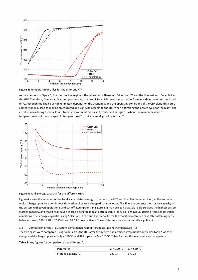
Figure 3: Temperature profiles for the different HTF

As may be seen in Figure 3, the thermocline region is the widest with Therminol 66 as the HTF and the thinnest with Solar Salt as the HTF. Therefore, from stratification’s perspective, the use of Solar Salt results in better performance than the other simulated HTFs. Although the choice of HTF ultimately depends on the economics and the operating conditions of the CSP plant, this sort of comparison may lead to making an educated decision with respect to the HTF when optimising the power cycle for the plant. The effect of considering thermal losses to the environment may also be observed in Figure 3 where the minimum value of temperature is not the storage cold temperature (Tc), but a value slightly lower than Tc.

Figure 4: Tank storage capacity for the different HTFs

Figure 4 shows the variation of the total accumulated energy in the tank (the HTF and the filler bed combined) at the end of a typical charge cycle for a continuous simulation of several charge-discharge loops. This figure represents the storage capacity of the system with given operational and cut-off assumptions. In Figure 4, it may be seen that Solar Salt provides the highest system storage capacity, and that it took seven charge-discharge loops to attain stable (or cyclic) behaviour, starting from similar initial conditions. The storage capacities using Solar Salt, HITEC and Therminol 66 for the modified reference case after attaining cyclic behaviour were 120.17 GJ, 107.25 GJ and 92.63 GJ respectively. These differences are economically significant.

3.3 Comparison of the TTES system performance with different storage hot temperature (Th) The two cases were compared using Solar Salt as the HTF after the system had attained cyclic behaviour which took 7 loops of charge and discharge cycles with Th = 390 °C, and 48 loops with Th = 560 °C. Table 3 shows the key results for comparison.

Table 3: Key figures for comparison using different Th

Parameter Th = 390 °C Th = 560 °C

Storage capacity (GJ) 120.17 179.26

8

Parameter Th = 390 °C Th = 560 °C

Charge cycle duration (h) 6.04 3.44

Discharge cycle duration (h) 5.52 3.03 From Table 3, it may be observed that the storage capacity of the tank is larger for the higher value of Th. This happens because a significantly larger amount of energy was supplied to the storage system as a direct result of operating with a much higher storage hot temperature. However, as will be shown later, there is no straight relation between the storage capacity and the storage hot temperature as the cut-off temperature difference also plays a significant role. It may also be observed that the there is a difference between the duration of the charge cycle and its corresponding discharge cycle for both the storage hot temperatures. This difference is a consequence of the relatively larger amount thermal losses to the ambient during the discharge cycle than during the charge cycle, when considering the same cut-off criterion for both the cycles.

3.4 Comparison of the TTES system performance with change in the cut-off temperature difference The cut-off temperature difference was changed to 10 °C and 30 °C while using Solar Salt as the HTF, for two values of the storage hot temperature (i.e. for Th = 390 °C and 560 °C). The storage cold temperature Tc was kept constant at 290 °C for all the cases. The TTES system performance was investigated with respect to the change in the cut-off temperature difference after the system had attained cyclic behaviour. The key results are shown in Table 4.

Table 4: Key figures for comparison using different values of the cut-off temperature difference

Parameter Cut-off temperature difference

Th = 390 °C Th = 560 °C

Storage capacity (GJ) 10 70.58 36.28 20 120.17 179.26 30 139.58 254.61

Charge cycle duration (h)

10 3.63 0.70 20 6.04 3.44 30 6.96 4.86

Discharge cycle duration (h)

10 3.12 0.63 20 5.52 3.03 30 6.53 4.34

From Table 4, it may be observed that with increasing value of the cut-off temperature difference, the durations of both the charge and the discharge cycles increase. This might be expected as increasing cut-off temperature difference allows for the tank to operate for a longer duration. As might also be expected, the storage capacity of the tank also increases with the cut-off temperature difference.

4 Discussion The presented model demonstrates the effect of considering the cyclic behaviour of the storage system and the time required to attain stability which directly influences the response time of the storage system, its discharge rate and storage capacity. The results from the simulations for a reference case have been validated against the experimental observations made by Pacheco et al. (Pacheco et al. 2002). The model may thus be regarded as simplified yet sufficiently accurate to predict system performance without being computationally intensive. As mentioned earlier, it was observed that the duration of the charge cycle is different than that of the corresponding discharge cycle (see Table 3). This difference is a direct influence of considering the cut-off criterion for the charge and the discharge cycles, and the thermal loss to the ambient. The higher thermal loss during the discharge cycle is because a larger volume of the tank is filled with HTF at the storage hot temperature, thus creating a higher average temperature difference between the HTF and the ambient. Since the cut-off criterion for both the charge and the discharge cycles was the same, the higher thermal loss resulted in attaining the cut-off temperature sooner for the discharge cycle than its corresponding charge cycle, and hence a lesser duration for the discharge cycle than its corresponding charge cycle. Most previous studies have either considered equal durations for both charge and discharge cycles, or have not considered this aspect at all. The present model thus brings the analysis closer to reality, as the cycle durations are related to the fluid outlet conditions. The cut-off criterion for a discharge cycle depends upon the application, while for the charge cycle it also depends upon the plant layout. Thus, while modelling the storage system, it is important to know the operating conditions from both the collector and the load sides. This was considered by using relevant boundary conditions for CSP plants as mentioned in Section 1. Until now, most of the publications dealt with the thermal behaviour of a thermocline tank in isolation. To study the tank performance as a part of the entire power cycle including both the solar receiver and the power block, the current model will be

9

useful as it would include variation in cycle durations for the charge and the discharge cycles, and predict the power cycle behaviour during the start-up of the storage system. At the same time, it is also important to consider this behaviour during everyday operation. This consideration would assist the designer size the solar field and the storage tank, depending on the sun hours available for charging and the storage capacity requirement. For a TTES system operating with higher value of storage hot temperature with the cut-off temperature difference set at 20 °C, even when the duration of a typical charge or discharge cycle was much lower, it took more time for the tank to attain cyclic behaviour (312.7 h with Th = 560 °C as compared with 84.69 h with Th = 390 °C). From Table 4, it may be observed that the storage capacity of the tank is highly sensitive to not only the cut-off temperature difference, but also the storage hot temperature. The storage capacity sees a much larger variation with a higher value of Th. It should be noted that the storage cold temperature (Tc) was kept constant at 290 °C for all the cases. Thus, it may be concluded that along with the storage temperature difference (i.e. Th - Tc), the most initial conditions also play a role in the TTES system performance with respect to the time required to attain the cyclic behaviour. This is important as a CSP plant is bound to shut down during long low irradiation periods even if a storage system is employed. During these shut-downs, it is not necessary that it will take the same amount of time for the TTES system to attain cyclic behaviour as it took in the beginning when the TTES system was put into operation for the first time. Therefore, when designing a storage system for particular operating conditions depending on the application of interest, it is important to consider the relative importance of storage capacity and the stability criteria such as cycle duration and cyclic behaviour.

5 Conclusion A one-dimensional transient model for TTES system was developed. The model assumes local thermal non-equilibrium between the HTF and the filler bed, variation in the thermophysical properties of the HTF with temperature and the effect of heat loss from the tank walls using an overall heat loss coefficient. The presented model was carefully verified based on grid refinement and time step independence studies, and validated against experimental data by Pacheco et al. (Pacheco et al. 2002). The main observations from the analysis are presented below. These findings are important in sizing a storage tank based on the power cycle operational requirements such as storage capacity, discharge power and flow rate.

• The cyclic behaviour of the system was found to be attained only after several charge-discharge loops. The cyclic temperature profiles and the storage capacity depended upon the type of HTF used and the storage temperature difference, but not on the initial conditions (i.e. the temperature distribution of the HTF and the filler bed at the beginning of the first charge cycle).

• From stratification perspective, Solar Salt performs the best from the three compared HTFs. • The effect of the temperature difference between the hot fluid and the cold fluid in the storage system has a great

impact on system stability (i.e. the system takes longer to attain cyclic behaviour even when the duration of individual cycles is smaller for higher temperature differences).

• The difference in the durations of the charge cycle and its corresponding discharge cycle can be attributed to the consideration of similar cycle cut-off criterion and thermal losses to the ambient.

• The storage capacity of the tank is highly sensitive to both the cycle cut-off criteria and the storage temperature difference.

Acknowledgements The first author gratefully acknowledges the financial support received from the Erasmus Mundus and EIT KIC InnoEnergy SELECT program. David Wyon is thanked for proofreading the manuscript and suggesting improvements.

Nomenclature Characters aloss Tank wall area per unit volume, m-1 C Isobaric specific heat capacity, J/kg-K D Tank diameter, m Dp Filler bed particle diameter, m H Tank height, m hv Volumetric heat transfer coefficient, W/m3-K k Thermal conductivity, W/m-K ṁ Mass flow rate, kg/s

10

N Number of control volumes Pr Prandtl number ReP Reynolds number based on particle diameter T Temperature, K t Time, s Uloss Overall heat loss coefficient for tank wall, W/m2-K w Darcy or superficial velocity, m/s Δz Grid height for simulations, m Abbreviations and acronyms CSP Concentrated solar power CV Control volume HTF Heat transfer fluid TES Thermal energy storage TTES Thermocline thermal energy storage Greek letters ε Filler bed porosity ρ Density, kg/m3 Subscripts b Filler bed property c Fluid cold state ext Ambient or external property f Heat transfer fluid property h Fluid hot state

References Barlev, D., Vidu, R. & Stroeve, P., 2011. Innovation in concentrated solar power. Solar Energy Materials and Solar Cells, 95(10),

pp.2703–2725. Bayón, R. & Rojas, E., 2013. Simulation of thermocline storage for solar thermal power plants: From dimensionless results to

prototypes and real-size tanks. International Journal of Heat and Mass Transfer, 60, pp.713–721. Brosseau, D. et al., 2005. Testing of Thermocline Filler Materials and Molten-Salt Heat Transfer Fluids for Thermal Energy Storage

Systems in Parabolic Trough Power Plants. Journal of Solar Energy Engineering, 127(1), pp.109–116. Dincer, I. & Dost, S., 1996. A perspective on thermal energy storage systems for solar energy applications. International Journal of

Energy Research, 20, pp.547–557. Fernández-García, A. et al., 2010. Parabolic-trough solar collectors and their applications. Renewable and Sustainable Energy

Reviews, 14(7), pp.1695–1721. Flueckiger, S., Yang, Z. & Garimella, S. V., 2011. An integrated thermal and mechanical investigation of molten-salt thermocline

energy storage. Applied Energy, 88(6), pp.2098–2105. Flueckiger, S.M. et al., 2014. System-level simulation of a solar power tower plant with thermocline thermal energy storage.

Applied Energy, 113, pp.86–96. Flueckiger, S.M., Yang, Z. & Garimella, S. V., 2012. Thermomechanical Simulation of the Solar One Thermocline Storage Tank.

Journal of Solar Energy Engineering, 134(4), p.041014. Gil, A. et al., 2010. State of the art on high temperature thermal energy storage for power generation. Part 1—Concepts, materials

and modellization. Renewable and Sustainable Energy Reviews, 14(1), pp.31–55. Greenpeace International, SolarPACES & ESTELA, 2009. Concentrating Solar Power: Global Outlook 2009, International Energy Agency, 2010. Technology Roadmap: Concentrating Solar Power, OECD Publishing. Karaki, W. et al., 2010. Heat transfer in thermocline storage system with filler materials: Analytical model. In Proceedings of the

ASME 2010 4th International Conference on Energy Sustainability. Phoenix, Arizona, USA: ASME, pp. 1–10. Van Lew, J.T. et al., 2011. Analysis of Heat Storage and Delivery of a Thermocline Tank Having Solid Filler Material. Journal of Solar

Energy Engineering, 133(2), p.021003. Van Lew, J.T. et al., 2009. Transient heat delivery and storage process in a thermocline heat storage system. In 2009 International

Mechanical Energineering Congress & Exposition. Lake Buena Vista, Florida: ASME, pp. 1–10. Li, P. et al., 2011. Generalized charts of energy storage effectiveness for thermocline heat storage tank design and calibration. Solar

Energy, 85(9), pp.2130–2143.

11

Pacheco, J.E., Showalter, S.K. & Kolb, W.J., 2002. Development of a Molten-Salt Thermocline Thermal Storage System for Parabolic Trough Plants. Journal of Solar Energy Engineering, 124(2), p.153.

Schumann, T.E.W., 1929. Heat transfer: A liquid flowing through a porous prism. Journal of the Franklin Institute, 208(3), pp.405–416.

SOLUTIA, 2013. Therminol 66. Available at: http://twt.mpei.ac.ru/TTHB/HEDH/HTF-66.PDF [Accessed July 29, 2013]. Tesfay, M. & Venkatesan, M., 2013. Simulation of thermocline thermal energy storage system using C. International Journal of

Innovation and Applied Studies, 3(2), pp.354–364. Valmiki, M.M. et al., 2012. Experimental investigation of thermal storage processes in a thermocline tank. Journal of Solar Energy

Engineering, 134(4), p.041003. Xu, C. et al., 2013. Effects of solid particle properties on the thermal performance of a packed-bed molten-salt thermocline thermal

storage system. Applied Thermal Engineering, 57(1-2), pp.69–80. Xu, C. et al., 2012a. Parametric study and standby behavior of a packed-bed molten salt thermocline thermal storage system.

Renewable Energy, 48, pp.1–9. Xu, C. et al., 2012b. Sensitivity analysis of the numerical study on the thermal performance of a packed-bed molten salt

thermocline thermal storage system. Applied Energy, 92, pp.65–75. Yang, Z. & Garimella, S. V., 2013. Cyclic operation of molten-salt thermal energy storage in thermoclines for solar power plants.

Applied Energy, 103, pp.256–265. Yang, Z. & Garimella, S. V., 2010a. Molten-salt thermal energy storage in thermoclines under different environmental boundary

conditions. Applied Energy, 87(11), pp.3322–3329. Yang, Z. & Garimella, S. V., 2010b. Thermal analysis of solar thermal energy storage in a molten-salt thermocline. Solar Energy,

84(6), pp.974–985. Zavoico, A.B., 2001. Solar power Tower: Design basis document, San Francisco, California.

Appendix The correlations for thermophysical properties of HITEC molten salt (Yang & Garimella 2010b) and Therminol 66 (SOLUTIA 2013) are given in Tables A1 and A2 respectively. For simplification, it was assumed that the same relations would hold true for ±10% of the operating temperature range as specified by the manufacturer. Table A1: Correlations for thermophysical properties of HITEC molten salt, T (K) Density kg/m3 1938 – 0.732 (T – 200) Specific heat capacity J/kg-K 1561.7 (nearly constant for operating temperature range) Absolute viscosity kg/m-s exp [-4.343 – 2.0143 {ln (T) – 5.011}] Thermal conductivity W/m-K 0.421 – 0.000653 (T – 260)

Table A2: Correlations for thermophysical properties of Therminol 66, T (K) Density kg/m3 1164.45 – 0.4389 T – 3.21·10-4 T2 Specific heat capacity J/kg-K 658 + 2.82 T + 8.97·10-4 T2 Absolute viscosity kg/m-s (1164.45 – 0.4389 T – 3.21·10-4 T2) · exp [-16.096 + {586.38 / (T – 210.65)}] Thermal conductivity W/m-K 0.116 + 4.9·10-5 T – 1.5·10-7 T2