thermal and pore pressure history of the haynesville shale
TRANSCRIPT
Louisiana State UniversityLSU Digital Commons
LSU Master's Theses Graduate School
2012
Thermal and pore pressure history of theHaynesville Shale in north Louisiana: a numericalstudy of hydrocarbon generation, overpressure, andnatural hydraulic fracturesWilliam C. TorschLouisiana State University and Agricultural and Mechanical College
Follow this and additional works at: https://digitalcommons.lsu.edu/gradschool_theses
Part of the Earth Sciences Commons
This Thesis is brought to you for free and open access by the Graduate School at LSU Digital Commons. It has been accepted for inclusion in LSUMaster's Theses by an authorized graduate school editor of LSU Digital Commons. For more information, please contact [email protected].
Recommended CitationTorsch, William C., "Thermal and pore pressure history of the Haynesville Shale in north Louisiana: a numerical study of hydrocarbongeneration, overpressure, and natural hydraulic fractures" (2012). LSU Master's Theses. 268.https://digitalcommons.lsu.edu/gradschool_theses/268

THERMAL AND PORE PRESSURE HISTORY OF THE HAYNESVILLE SHALE IN NORTH LOUISIANA: A NUMERICAL STUDY OF HYDOCARBON GENERATION,
OVERPRESSURE, AND NATURAL HYDRAULIC FRACTURES
A Thesis
Submitted to the Graduate Faculty of the Louisiana State University and
Agricultural and Mechanical College in partial fulfillment of the
Requirements for the degree of Masters of Science
in
The Department of Geology and Geophysics
by William Cross Torsch
B.S., Baylor University, 2010 December 2012

ii
Acknowledgments I would like to thank my advisory Dr. Jeffrey Nunn for mentoring me at
Louisiana State University and for guidance in the classroom and research. I would also
like to thank my committee members Dr. Jeffrey Hanor and Dr. Arash Dahi for their help
and support. I would like to thank Marathon Oil and the LSU Department of Geology
and Geophysics for financial support. Additionally, thanks to Halliburton and
Schlumberger for software donations.
Special thanks to Richard Campbell of Edgewood Exploration for mentoring me
in the field of petroleum geology and sharing his knowledge of the geology of south
Louisiana. Thanks to my fellow students in the Department of Geology and Geophysics.
Lastly, I would like to thank the faculty and staff at Baylor University for providing me
with a strong foundation that enabled me to achieve my goals at LSU.

iii
Table of Contents Acknowledgments ............................................................................................................... ii
List of Tables ....................................................................................................................... v
List of Figures .................................................................................................................... vi
Abstract .............................................................................................................................. ix
Chapter 1. Introduction ....................................................................................................... 1
Chapter 2. Geologic Overview ............................................................................................ 2
2.1 Study Area ................................................................................................................. 2
2.2 Tectonic Framework ................................................................................................. 3
2.3 The Haynesville Shale ............................................................................................... 5
2.4 Fluid Overpressure .................................................................................................. 11
2.5 Hydraulic Fractures ................................................................................................. 12
Chapter 3. Data and Methods ............................................................................................ 14
3.1 Data ......................................................................................................................... 14
3.2 Well Tops and Lithologies ...................................................................................... 14
3.3 Modeling ................................................................................................................. 17
3.4 Geologic Ages ......................................................................................................... 18
3.5 Erosion Estimates .................................................................................................... 20
3.6 Present Day Heat Flow ............................................................................................ 21
3.7 Paleoheat Flow ........................................................................................................ 23
3.8 Thermal Maturity .................................................................................................... 24
3.9 Porosity and Pressure .............................................................................................. 25
3.10 Paleowater Depths and Sediment Water Interface Temperature .......................... 26
Chapter 4. Results ............................................................................................................. 27
4.1 Thermal Maturation................................................................................................. 27
4.2 Fluid Pressure .......................................................................................................... 28
4.3 Fluid Migration ....................................................................................................... 31
Chapter 5. Discussion ....................................................................................................... 46
iv
5.1 Sensitivity Studies ................................................................................................... 46
5.2 Fluid Pressure Transfer ........................................................................................... 57
5.3 Hydrocarbon Migration ........................................................................................... 60
5.4 Natural Hydraulic Fractures .................................................................................... 65
Chapter 6. Conclusions ..................................................................................................... 67
References ......................................................................................................................... 69
Appendix A. Well Tops ................................................................................................... 75
Appendix B. Basin Modeling ........................................................................................... 76
Appendix C. Thermal Maturity ......................................................................................... 81
Vita .................................................................................................................................... 82

v
List of Tables Table 1:. Lithologies used for modeling ........................................................................... 17
Table 2: Cenozoic and Mesozoic unconformities of north Louisiana ............................. 21
Table B1:. Fundamental physical transport laws and variables ........................................ 80
vi
List of Figures Figure 1: Map showing the locations of the Gulf Coast sub-basins.................................... 2
Figure 2: Structural elements of the northern Gulf of Mexico ............................................ 4
Figure 3: Model of crust from gravity data along a north-south line through the Sabine Uplift along the Texas-Louisiana border ............................................................................ 5
Figure 4: Stratigraphic column for north Louisiana ............................................................ 6
Figure 5: Pressure contour map of the Haynesville Shale from well test data .................... 9
Figure 6: Twenty feet of image log showing natural fractures at mid level position in Haynesville Shale. Well is located in DeSoto Parish ........................................................ 10
Figure 7: Map of north Louisiana with well control shown by circles ............................. 15
Figure 8: Type log for north Louisiana ............................................................................. 16
Figure 9: Discretization of 2 D models ............................................................................. 19
Figure 10: Eroded thickness of the missing Cretaceous section and well locations ......... 22
Figure 11: North America heat flow map ......................................................................... 23
Figure 12: Paleo heat flow models used in this study ....................................................... 25
Figure 13: . Map of study area indicating the locations of the four wells shown in the results and discussion sections .......................................................................................... 28
Figure 14: Burial history plots with EASY Ro% overlay ................................................. 29
Figure 15: Plot of vitrinite reflectance vs. time for four wells .......................................... 30
Figure 16: 1D pressure versus depth models for 1 Gish, 1 Cates, 1 Foster, and C1 Tremont wells .................................................................................................................... 32
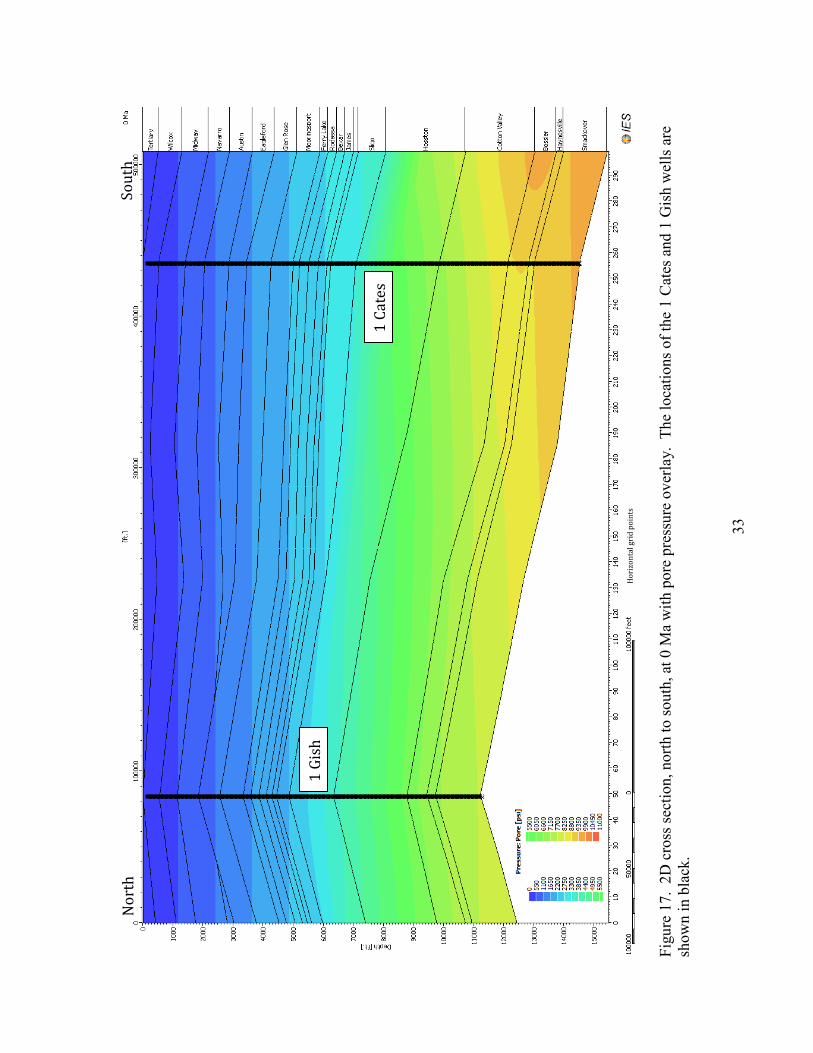
Figure 17: 2D cross section, north to south, at 0 Ma with pore pressure overlay ............. 33

vii
Figure 18: 2D cross section, west to east, at 0 Ma with pore pressure overlay ................ 34
Figure 19: Pore pressure versus depth at 0 Ma extracted from 2D models ...................... 35
Figure 20: Pore and fracture pressures versus time. Extractions from 2D models .......... 36
Figure 21: 2D cross section, north to south, at 87 Ma with pore pressure overlay ........... 37
Figure 22: 2D cross section, west to east, at 87 Ma with pore pressure overlay .............. 38
Figure 23: 2D cross section, north to south, at 0 Ma with pore pressure overlay. Haynesville Shale gas (red) and oil (green) migration pathways indicated by arrows ..... 39
Figure 24: 2D cross section, west to east, at 0 Ma with pore pressure overlay. Haynesville Shale gas (red) and oil (green) migration pathways indicated by arrows ..... 41
Figure 25: 2D cross section, north to south, at 87 Ma with pore pressure overlay. Haynesville Shale gas (red) and oil (green) migration pathways indicated by arrows ..... 42
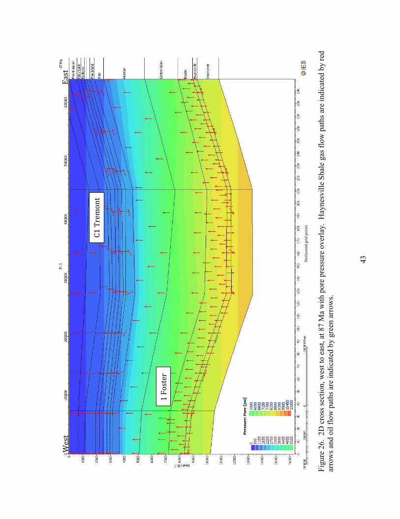
Figure 26: 2D cross section, west to east, at 87 Ma with vertical permeability overlay. Haynesville Shale gas (red) and oil (green) migration pathways indicated by arrows ..... 43
Figure 27: 2D cross sections from north to south and east to west at 0 Ma with vertical permeability overlay. Blue arrows represent water flow pathways ................................. 44
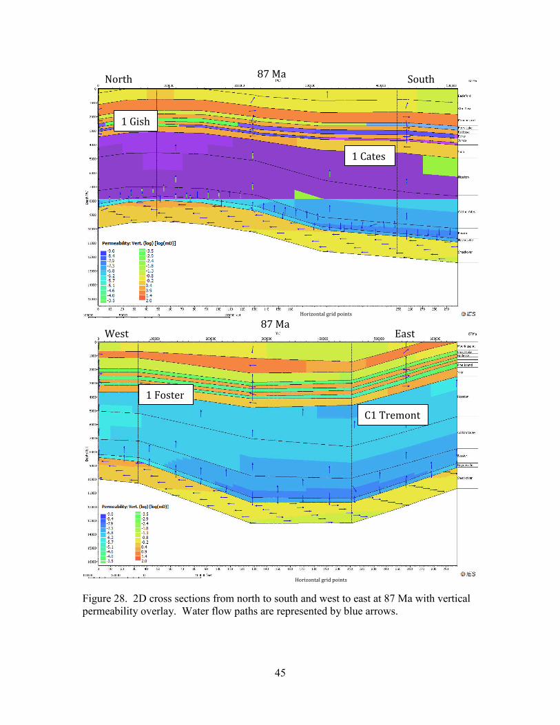
Figure 28: 2D cross sections from north to south and east to west at 87 Ma with vertical permeability overlay. Blue arrows represent water flow pathways ................................. 45
Figure 29: . Haynesville hydrocarbon generation pressure versus time extracted from 2D models at the 1-Gish and 1-Cates wells ............................................................................ 47
Figure 30: Pressure increase due to hydrocarbon generation in the north to south cross-section at 105 and 88 Ma................................................................................................... 48
Figure 31: Pressure increase due to hydrocarbon generation in the north to south cross-section at 87 and 85 Ma..................................................................................................... 49
Figure 32: Pressure versus depth for variable permeabilities of the Hosston, Cotton Valley, and Bossier formations ......................................................................................... 51

viii
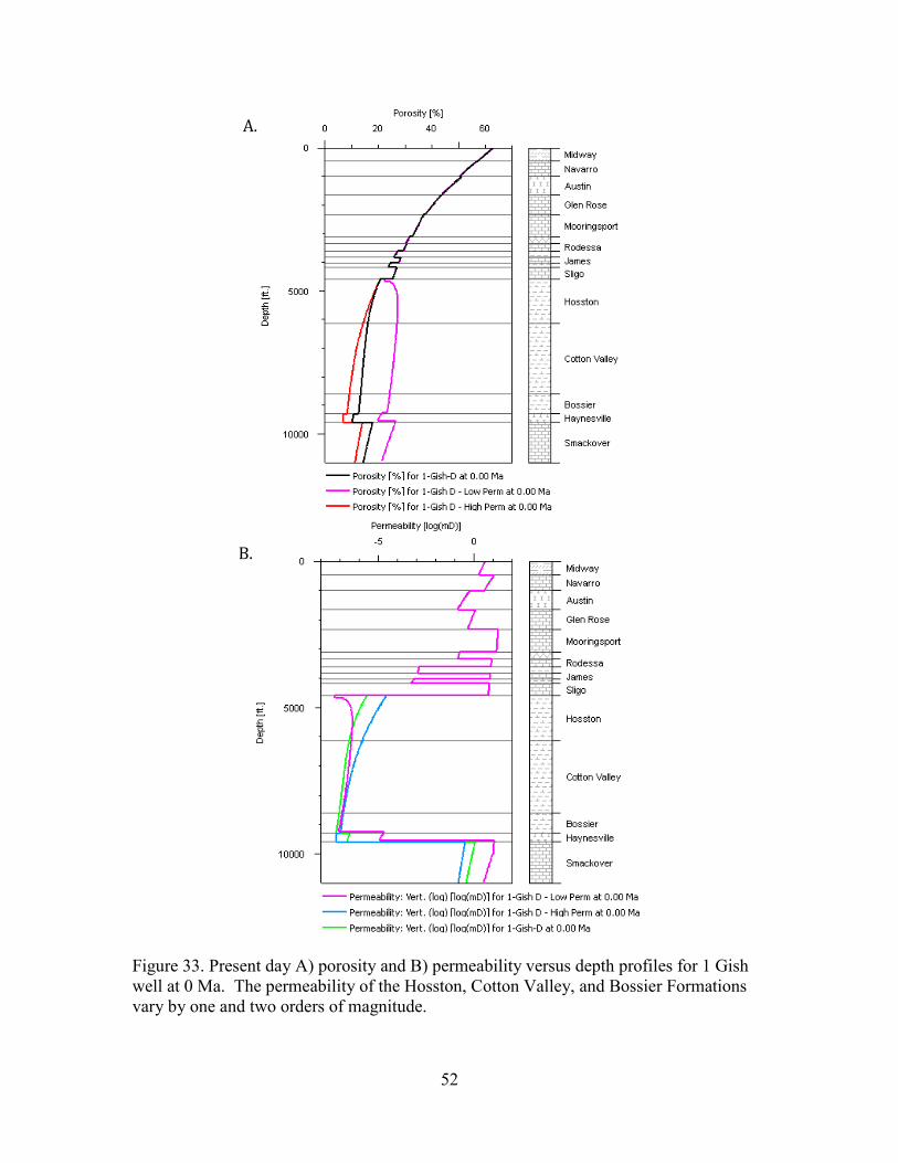
Figure 33: Porosity and permeability versus depth profile for 1 Gish well at 0 Ma. The permeability of the Hosston, Cotton Valley, and Bossier Formations vary by one and two orders of magnitude. .......................................................................................................... 52
Figure 34: Cross section B-B’ with pressure overlay and arrows indicating direction of gas (red) and oil (green) migration. Smackover Limestone permeability values are one order of magnitude less those used in final model. ........................................................... 54
Figure 35: Cross section B-B’ with pressure overlay and arrows indicating direction of gas (red) and oil (green) migration. Smackover Limestone permeability values are two orders of magnitude less those used in final model. ......................................................... 55
Figure 36: Pressure versus depth for the 1 Gish D well at 0 Ma for 0 ft, 500 ft, and 1500 ft of Eocene erosion. ........................................................................................................ 56
Figure 37: Smackover and Haynesville hydrocarbon generation pressure in the north to south cross section at 105 and 88 Ma. ............................................................................... 58
Figure 38: Smackover and Haynesville hydrocarbon generation pressure in the north to south cross section at 87 and 85 Ma. ................................................................................. 59
Figure 39: Present day pore pressure comparison of 1D vs 2D models for 1-Gish well .. 61
Figure 40: Present day pore pressure comparison of 1D vs 2D models for 1-Cates well . 61
Figure 41: Present day pore pressure comparison of 1D vs 2D models for 1-Foster well 62
Figure 42: Present day pore pressure comparison of 1D vs 2D models for C1-Tremont well .................................................................................................................................... 62
Figure 43: Smackover structure map at 0 Ma. Red arrows indicate the direction of fluid migration. Well control is shown by black dots ............................................................... 63
Figure 44: Smackover structure map at 0 Ma. Red arrows indicate the direction of fluid migration. Well control is shown by black dots ............................................................... 66
Figure B1: Major geologic processes in basin modeling .................................................. 77
Figure B2: Process workflow diagram for numerical basin modeling.............................. 78
ix
Abstract
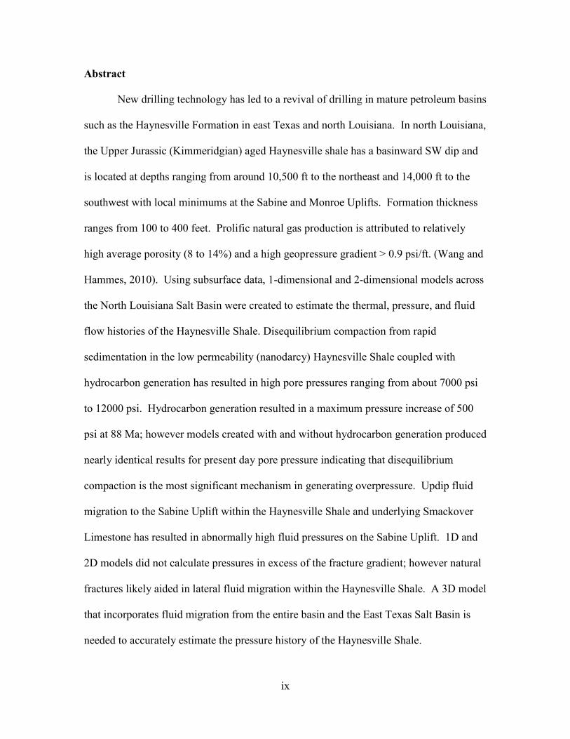
New drilling technology has led to a revival of drilling in mature petroleum basins
such as the Haynesville Formation in east Texas and north Louisiana. In north Louisiana,
the Upper Jurassic (Kimmeridgian) aged Haynesville shale has a basinward SW dip and
is located at depths ranging from around 10,500 ft to the northeast and 14,000 ft to the
southwest with local minimums at the Sabine and Monroe Uplifts. Formation thickness
ranges from 100 to 400 feet. Prolific natural gas production is attributed to relatively
high average porosity (8 to 14%) and a high geopressure gradient > 0.9 psi/ft. (Wang and
Hammes, 2010). Using subsurface data, 1-dimensional and 2-dimensional models across
the North Louisiana Salt Basin were created to estimate the thermal, pressure, and fluid
flow histories of the Haynesville Shale. Disequilibrium compaction from rapid
sedimentation in the low permeability (nanodarcy) Haynesville Shale coupled with
hydrocarbon generation has resulted in high pore pressures ranging from about 7000 psi
to 12000 psi. Hydrocarbon generation resulted in a maximum pressure increase of 500
psi at 88 Ma; however models created with and without hydrocarbon generation produced
nearly identical results for present day pore pressure indicating that disequilibrium
compaction is the most significant mechanism in generating overpressure. Updip fluid
migration to the Sabine Uplift within the Haynesville Shale and underlying Smackover
Limestone has resulted in abnormally high fluid pressures on the Sabine Uplift. 1D and
2D models did not calculate pressures in excess of the fracture gradient; however natural
fractures likely aided in lateral fluid migration within the Haynesville Shale. A 3D model
that incorporates fluid migration from the entire basin and the East Texas Salt Basin is
needed to accurately estimate the pressure history of the Haynesville Shale.

1
Chapter 1. Introduction The Upper Jurassic (Kimmeridgian) Haynesville Shale is a prolific natural gas
producing rock that has led to the revival of exploration and drilling in the heavily
explored North Louisiana Salt Basin and East Texas Salt Basin (Figure 1) (Mancini et
al, 2005). New drilling and completion techniques allow companies to produce
hydrocarbons directly from the source rock. The Haynesville is a particularly
attractive shale gas play because of high overpressures (Wang and Hammes, 2010).
High overpressures tend to enhance the porosity, gas content, and apparent
brittleness of gas shales (Wang and Hammes, 2010). The pore pressure of the
Haynesville is near the fracture pressure. Low effective stress makes the
Haynesville easy to hydraulically fracture using modern well completion techniques.
(Wang and Lui, 2011)
The Haynesville Shale consists of a dark, organic rich, mudstone-marl facies
with ubiquitous pyrite (Buller and Dix, 2009). The Haynesville is known to contain
natural hydraulic fractures that have been mineralogically healed as a result of fluid
flow (Buller and Dix, 2009). Disequilibrium compaction coupled with hydrocarbon
generation can result in significant overpressures in low permeability (nanodarcy)
rocks (Swarbrick et al, 2002) such as the Haynesville Shale. The purpose of this
study is to use 1D and 2D basin models to estimate the burial, thermal, maturation,
pore pressure, and fluid migration history of the Haynesville Shale to further our
understanding of the distribution of overpressures and the propagation of natural
hydraulic fractures (Nunn et al., 1984; Li, 2006; Mancini et al., 2008).

2
Chapter 2. Geologic Overview
2.1 Study Area
The Haynesville Shale gas play occurs over a broad area covering the East Texas
Salt Basin and the North Louisiana Salt Basin. This study is confined to north Louisiana
(Figure 1). The main play occurs over the Sabine Uplift corresponding to relatively
shallower Jurassic strata and high gas production (Hammes et al., 2011). The initial
basin architecture and extensional history created a series of high standing basement
blocks separated by areas of more extended crust influencing the distribution and
deposition of salt and younger Jurassic rocks. Cretaceous uplift likely affected thermal
history, burial history, and thermal maturity of the basin (Hammes et al., 2011).
Figure 1. Map showing the locations of the Gulf Coast sub-basins. The study area is shown in red (modified after Mancini et al., 2005).
3
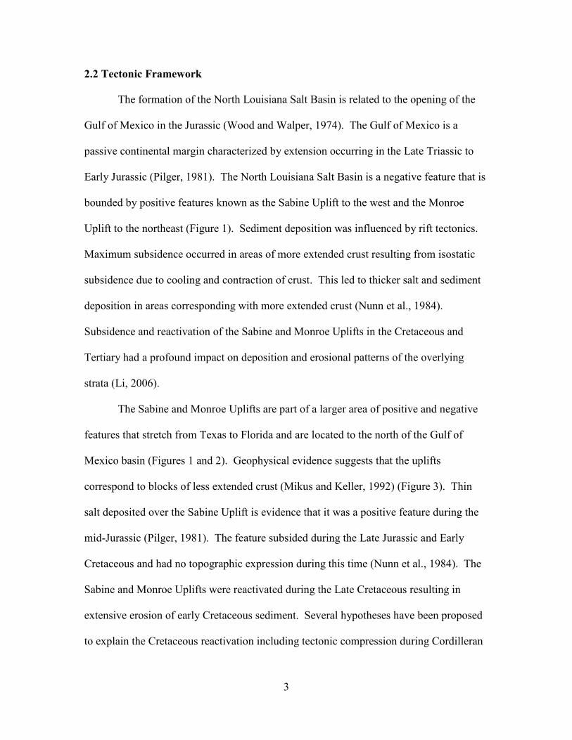
2.2 Tectonic Framework
The formation of the North Louisiana Salt Basin is related to the opening of the
Gulf of Mexico in the Jurassic (Wood and Walper, 1974). The Gulf of Mexico is a
passive continental margin characterized by extension occurring in the Late Triassic to
Early Jurassic (Pilger, 1981). The North Louisiana Salt Basin is a negative feature that is
bounded by positive features known as the Sabine Uplift to the west and the Monroe
Uplift to the northeast (Figure 1). Sediment deposition was influenced by rift tectonics.
Maximum subsidence occurred in areas of more extended crust resulting from isostatic
subsidence due to cooling and contraction of crust. This led to thicker salt and sediment
deposition in areas corresponding with more extended crust (Nunn et al., 1984).
Subsidence and reactivation of the Sabine and Monroe Uplifts in the Cretaceous and
Tertiary had a profound impact on deposition and erosional patterns of the overlying
strata (Li, 2006).
The Sabine and Monroe Uplifts are part of a larger area of positive and negative
features that stretch from Texas to Florida and are located to the north of the Gulf of
Mexico basin (Figures 1 and 2). Geophysical evidence suggests that the uplifts
correspond to blocks of less extended crust (Mikus and Keller, 1992) (Figure 3). Thin
salt deposited over the Sabine Uplift is evidence that it was a positive feature during the
mid-Jurassic (Pilger, 1981). The feature subsided during the Late Jurassic and Early
Cretaceous and had no topographic expression during this time (Nunn et al., 1984). The
Sabine and Monroe Uplifts were reactivated during the Late Cretaceous resulting in
extensive erosion of early Cretaceous sediment. Several hypotheses have been proposed
to explain the Cretaceous reactivation including tectonic compression during Cordilleran

thrust faulting in western North America (Jackson and Laubach, 1988; Laub
Jackson, 1990) and partial relaxation of the lithosphere due to buoyant crustal blocks of
different thicknesses (Nunn, 1
in Texas and northeastern Mexico
uplifts are a result of thermal
and Monroe Uplifts were reactivated during the Eocene as evidenced by thinning of the
Wilcox formation (Jackson and Laubach, 1988).
Figure 2. Structural elements of the northern Gulf of Mexico. basement in kilometers modified from Sawyer et al. (1991). Partial cross section Afor Figure 3 is shown. SU=Sabine Uplift; WU=Wiggins Uplift; MGA=Middle Ground Arch; SA=Sarasota Arch, ETSB=East Texas Salt Basin; NLSB=North Louisiana Salt Basin; MSB=Mississippi Salt Basin; Green lines are transform faults; dark orange=continental crust, light orange=thick transitional crust; light green = thin transitionaafter Hammes et al, 2011).
4
estern North America (Jackson and Laubach, 1988; Lauba
Jackson, 1990) and partial relaxation of the lithosphere due to buoyant crustal blocks of
different thicknesses (Nunn, 1990). However, lack of Cretaceous anticlinal development
in Texas and northeastern Mexico as well as the absence of strike slip faulting suggest
relaxation of the lithosphere (Ewing, 2009). The Sabine
reactivated during the Eocene as evidenced by thinning of the
n (Jackson and Laubach, 1988).
Figure 2. Structural elements of the northern Gulf of Mexico. Contours: depth to modified from Sawyer et al. (1991). Partial cross section A
for Figure 3 is shown. SU=Sabine Uplift; WU=Wiggins Uplift; MGA=Middle Ground Arch; SA=Sarasota Arch, ETSB=East Texas Salt Basin; NLSB=North Louisiana Salt Basin; MSB=Mississippi Salt Basin; DSSB=De Soto Salt Basin; TB=Tampa Basin. Green lines are transform faults; dark orange=continental crust, light orange=thick transitional crust; light green = thin transitional crust; purple = oceanic crust
ach and
Jackson, 1990) and partial relaxation of the lithosphere due to buoyant crustal blocks of
development
as well as the absence of strike slip faulting suggest the
The Sabine
reactivated during the Eocene as evidenced by thinning of the
depth to modified from Sawyer et al. (1991). Partial cross section A-A’
for Figure 3 is shown. SU=Sabine Uplift; WU=Wiggins Uplift; MGA=Middle Ground Arch; SA=Sarasota Arch, ETSB=East Texas Salt Basin; NLSB=North Louisiana Salt
DSSB=De Soto Salt Basin; TB=Tampa Basin. Green lines are transform faults; dark orange=continental crust, light orange=thick
(modified

Figure 3. Model of crust from gravity data along a northUplift along the Texas-Louisiana borderObserved gravity is represented by a triangle, and the calculated gravity isa plus symbol. (B) Interpretation of Crust. Numbers represent density in g/cm3. mi mafic intrusions (3.05 g/cm3)A-A’ shown in Figure 2.
2.3 The Haynesville Shale
The Late Jurassic (Kimme
Smackover Limestone (Figure 4)
dominated, matrix supported carbonate
grainstones of the Upper Smackover (
Overlying the Haynesville
Group consists of the Bossier, Cotton Valley, Hosston and Sligo Formation
Valley Formation is predominately shale interbedded with tight
porosity and 0.1 mD permeability) and limestone
5
Figure 3. Model of crust from gravity data along a north-south line through the Sabine Louisiana border. (A) Gravity data measured in Gal x 1000.
Observed gravity is represented by a triangle, and the calculated gravity is represented by a plus symbol. (B) Interpretation of Crust. Numbers represent density in g/cm3. mi mafic intrusions (3.05 g/cm3) (modified after Mickus and Keller, 1992). Line of section
Jurassic (Kimmeridgian) aged Haynesville Shale is underlain by the
(Figure 4). The lower Smackover consists of mudstone
dominated, matrix supported carbonates that grade upwards into packstones and
grainstones of the Upper Smackover (Presley and Reed, 1984).
Overlying the Haynesville Shale is the Cotton Valley Group. The Cotton Valley
the Bossier, Cotton Valley, Hosston and Sligo Formations. The C
ormation is predominately shale interbedded with tight sandstones (8
.1 mD permeability) and limestones (Zimmerman, 1999).
ine through the Sabine . (A) Gravity data measured in Gal x 1000.
represented by a plus symbol. (B) Interpretation of Crust. Numbers represent density in g/cm3. mi –
1992). Line of section
is underlain by the
mudstone
that grade upwards into packstones and
is the Cotton Valley Group. The Cotton Valley
s. The Cotton
sandstones (8-10 %

6
Figure 4. Stratigraphic column of north Louisiana (Li, 2006).
7
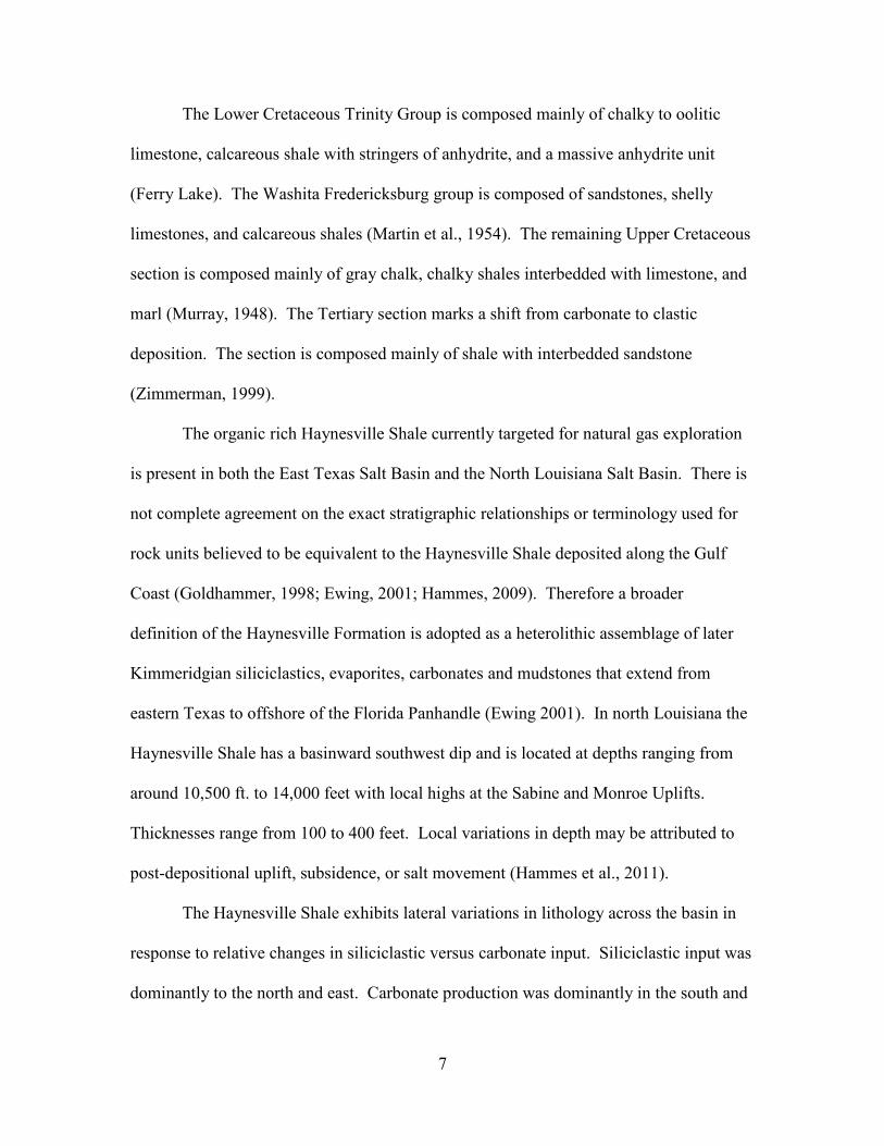
The Lower Cretaceous Trinity Group is composed mainly of chalky to oolitic
limestone, calcareous shale with stringers of anhydrite, and a massive anhydrite unit
(Ferry Lake). The Washita Fredericksburg group is composed of sandstones, shelly
limestones, and calcareous shales (Martin et al., 1954). The remaining Upper Cretaceous
section is composed mainly of gray chalk, chalky shales interbedded with limestone, and
marl (Murray, 1948). The Tertiary section marks a shift from carbonate to clastic
deposition. The section is composed mainly of shale with interbedded sandstone
(Zimmerman, 1999).
The organic rich Haynesville Shale currently targeted for natural gas exploration
is present in both the East Texas Salt Basin and the North Louisiana Salt Basin. There is
not complete agreement on the exact stratigraphic relationships or terminology used for
rock units believed to be equivalent to the Haynesville Shale deposited along the Gulf
Coast (Goldhammer, 1998; Ewing, 2001; Hammes, 2009). Therefore a broader
definition of the Haynesville Formation is adopted as a heterolithic assemblage of later
Kimmeridgian siliciclastics, evaporites, carbonates and mudstones that extend from
eastern Texas to offshore of the Florida Panhandle (Ewing 2001). In north Louisiana the
Haynesville Shale has a basinward southwest dip and is located at depths ranging from
around 10,500 ft. to 14,000 feet with local highs at the Sabine and Monroe Uplifts.
Thicknesses range from 100 to 400 feet. Local variations in depth may be attributed to
post-depositional uplift, subsidence, or salt movement (Hammes et al., 2011).
The Haynesville Shale exhibits lateral variations in lithology across the basin in
response to relative changes in siliciclastic versus carbonate input. Siliciclastic input was
dominantly to the north and east. Carbonate production was dominantly in the south and

8
west. Calcite content is controlled by erosion of nearby carbonate shoals (Goldhammer,
1998; Ewing 2001). The Haynesville shale is inferred to be more carbonate rich in the
south and southeast and more silica rich in the north and northwest (Buller and Dix,
2009). The Haynesville Shale is inferred to be more carbonate rich in north Louisiana
versus more clastic rich in east Texas.
A unique feature of the Haynesville Shale compared to other shale gas plays is
that it has abnormally high pressures (Wang and Liu, 2011). The pore pressure gradient
is about 0.9 psi/ft (Wang and Hammes, 2010), which is much higher than a normal
pressure gradient of 0.465 psi/ft. for typical Gulf Coast waters (Schlumberger Oilfield
Glossary). High pressures enhance porosity, gas content, and apparent brittleness in the
shale. Wang and Hammes (2010) estimated bottom hole pore pressures from well test
data (Figure 5). They observed that in Louisiana, Haynesville pore pressures exceeding
10,000 psi are found in Desoto and Red River Parishes and pore pressures decrease to the
north and south of this area.
Natural fractures play an important role in many shale plays (Gale et al., 2007;
Engelder et al., 2009). The Haynesville Shale is known to be brittle and naturally
fractured in some areas (Figure 6) (Buller and Dix, 2009). Very few natural fractures are
open and most are cemented with minerals such as calcite (Buller and Dix, 2009).
Although the Haynesville Shale is known to be hydraulically fractured, little research has
been made public as to the characterization or orientation of the fractures.
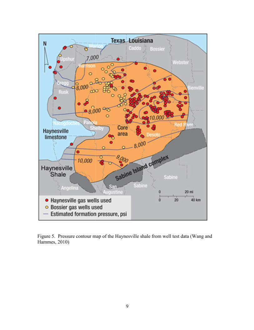
Figure 5. Pressure contour map of the Haynesville shale from well test data (Wang and Hammes, 2010)
9
map of the Haynesville shale from well test data (Wang and
map of the Haynesville shale from well test data (Wang and

10
Figure 6. Twenty feet of image log showing natural fractures at mid-level position in Haynesville Shale (Buller and Dix, 2009). The well is located in Desoto Parish, LA.

11
2.4 Fluid Overpressure
Much of the world’s oil and gas was generated from overpressured source rocks
(Hunt, 1990). If the pore pressure in a sedimentary rock is greater than the pressure
predicted by the weight of the overlying water column than it is referred to as
overpressured. Many theories have been proposed to explain the generation of
overpressures in sedimentary basins. The mechanisms that have the most impact on the
generation of overpressure in sedimentary basins are disequilibrium compaction,
hydrocarbon generation, or some combination of both (Swarbrick et al., 2002).
Disequilibrium compaction refers to the incomplete dewatering of low
permeability sediments during rapid sedimentation. Rapid sedimentation causes an
increase in vertical stress in a relatively short time span. Because the sediment does not
have adequate time to dewater, some portion of the weight of the increased load is
supported by the pore fluid (Swarbrick et al., 2002). Disequilibrium compaction will
result in sediments having greater pore pressure than the predicted hydrostatic pressure
(weight of the overlying water column) and a higher porosity relative to a normally
pressured and fully compacted rock. Disequilibrium compaction occurs at depth when
the permeability of the sediment is too low to allow for complete dewatering to occur.
According to Luo and Vasseur (1992) the main factors controlling the generation of
overpressure due to disequilibrium compaction are sedimentation rate, compaction
coefficient (rock “compressibility”), temperature, and permeability.
The conversion of kerogen to hydrocarbons may also play a role in the generation
of overpressure in sedimentary basins. Organic rich source rocks are exposed to
increasing temperatures as depth of burial increases which may convert kerogen to

12
hydrocarbons. The pore space in these source rocks becomes filled with petroleum and
water. Pore pressure will increase as the high-density kerogen in the source rocks is
converted into low-density hydrocarbons which results in an increase in volume.
Overpressure will occur as long as the rate of volume increase is faster than the rate of
fluid expulsion out of the source rock. (Guo et al., 2011).
2.5 Hydraulic Fractures A hydraulic fracture is a fracture that propagates as a result of the migration of
highly pressured fluid through a brittle rock (Hubbert and Willis 1957). It is important to
distinguish external hydraulic fractures from internal hydraulic fractures (Mandl and
Harkness 1987). External hydraulic fractures result from a fluid that originates from the
outside and penetrates an impermeable rock. This mechanism is used to explain the
migration of magmatic dikes and sills. Internal hydraulic fractures occur when
overpressured fluids migrate through the pore spaces within a rock and create fractures at
an internal point of weakness. This mechanism is generally used to explain mineral filled
veins in low permeability rocks. Primary migration of hydrocarbons through low-
permeability source rocks may be assisted by hydraulic fracture propagation (Nunn
1996).
The fracture pressures calculated in this study are the minimum pressure needed
for hydraulic fractures to propagate perpendicular to the least principal stress. In a
passive continental margin setting such as the North Louisiana Salt Basin, the least
effective stress is horizontal and fractures should be vertical (Sibson, 2003). The
Haynesville Shale may contain horizontal factures (J. A. Nunn, personal communication
2012). However, detailed fracture data are not yet available in the public domain.
13
Horizontal fractures within the Haynesville Shale may be explained by at least
one of the following conditions: 1) horizontal compression from tectonic forces, 2) high
susceptibility for fractures along bedding planes (anisotropic tensile strength) (Lash and
Engelder, 2005), or 3) vertical seepage forces from migrating fluid cause the least
principal stress to become vertical (Cobbold and Rodrigues, 2007).
14
Chapter 3. Data and Methods
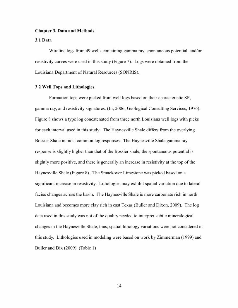
3.1 Data Wireline logs from 49 wells containing gamma ray, spontaneous potential, and/or
resistivity curves were used in this study (Figure 7). Logs were obtained from the
Louisiana Department of Natural Resources (SONRIS).
3.2 Well Tops and Lithologies
Formation tops were picked from well logs based on their characteristic SP,
gamma ray, and resistivity signatures. (Li, 2006; Geological Consulting Services, 1976).
Figure 8 shows a type log concatenated from three north Louisiana well logs with picks
for each interval used in this study. The Haynesville Shale differs from the overlying
Bossier Shale in most common log responses. The Haynesville Shale gamma ray
response is slightly higher than that of the Bossier shale, the spontaneous potential is
slightly more positive, and there is generally an increase in resistivity at the top of the
Haynesville Shale (Figure 8). The Smackover Limestone was picked based on a
significant increase in resistivity. Lithologies may exhibit spatial variation due to lateral
facies changes across the basin. The Haynesville Shale is more carbonate rich in north
Louisiana and becomes more clay rich in east Texas (Buller and Dixon, 2009). The log
data used in this study was not of the quality needed to interpret subtle mineralogical
changes in the Haynesville Shale, thus, spatial lithology variations were not considered in
this study. Lithologies used in modeling were based on work by Zimmerman (1999) and
Buller and Dix (2009). (Table 1)

15
Fi
gure
7.
Map
of n
orth
Lou
isia
na w
ith w
ell c
ontr
ol s
how
n by
cir
cles
.

16
SP Resistivity SP Resistivity
Figure 8. Type log for north Louisiana. The spontaneous potential curve in the left track and the resistivity curve in the right track. The type log is an aggradation of three wells located in north Louisiana. All logs are 1 inch with 100 ft. spacing. Logs were downloaded from the State of Louisiana Department of Natural Resources (sonris.com).
SP Resistivity
SP Resistivity
17
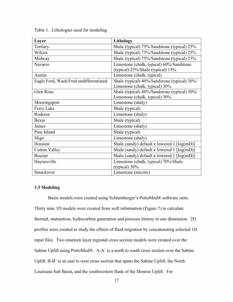
Table 1. Lithologies used for modeling Layer Lithology Tertiary Shale (typical) 75%/Sandstone (typical) 25% Wilcox Shale (typical) 75%/Sandstone (typical) 25% Midway Shale (typical) 75%/Sandstone (typical) 25% Navarro Limestone (chalk, typical) 60%/Sandstone
(typical) 25%/Shale (typical) 15% Austin Limestone (chalk, typical) Eagle Ford, Wash/Fred undifferentiated Shale (typical) 40%/Sandstone (typical) 30%/
Limestone (chalk, typical) 30% Glen Rose Shale (typical) 40%/Sandstone (typical) 30%/
Limestone (chalk, typical) 30% Mooringsport Limestone (shaly) Ferry Lake Shale (typical) Rodessa Limestone (shaly) Bexar Shale (typical) James Limestone (shaly) Pine Island Shale (typical) Sligo Limestone (shaly) Hosston Shale (sandy) default κ lowered 1 [log(mD)] Cotton Valley Shale (sandy) default κ lowered 1 [log(mD)] Bossier Shale (sandy) default κ lowered 1 [log(mD)] Haynesville Limestone (chalk, typical) 70%/Shale
(typical) 30% Smackover Limestone (micrite)
3.3 Modeling
Basin models were created using Schlumberger’s PetroMod® software suite.
Thirty nine 1D models were created from well information (Figure 7) to calculate
thermal, maturation, hydrocarbon generation and pressure history in one dimension. 2D
profiles were created to study the effects of fluid migration by concatenating selected 1D
input files. Two nineteen layer regional cross section models were created over the
Sabine Uplift using PetroMod®. A-A’ is a north to south cross section over the Sabine
Uplift. B-B’ is an east to west cross section that spans the Sabine Uplift, the North
Louisiana Salt Basin, and the southwestern flank of the Monroe Uplift. For

18
unconformities, stratigraphic thickness was restored to original thickness and removed
later as erosional events. 1D models were gridded using a maximum cell thickness of 20
m for all layers and a maximum time step duration of 1 Ma. 2D models were gridded
using a maximum vertical cell thickness of 20 m for the Haynesville layer, 50 m for the
Bossier and Smackover layers, and 400 m for the remaining layers. Running the models
with tighter grids for formations younger than the Bossier did not impact the
Haynesville’s geohistory and required significantly longer run times. 300 horizontal grid
points and maximum time step durations of 1 Ma were used in each 2D model (Figure 9).
Appendix B contains a more detailed explanation of the numerical modeling used in this
study.
3.4 Geologic Ages Stratigraphic intervals observed in well log data used in this study range from
Jurassic to Eocene in age. Geologic ages were assigned to the stratigraphic intervals
(Figure 4) using extensive biostratigraphic work done in the Gulf Coast region
summarized by Li (2006). Ages of the Tertiary units are from the work of Mancini and
Tew (1991). For the Upper Cretaceous strata, outcrop work of Christopher (1982),
Puckett (1985), Mancini et al. (1996), and the subsurface work of Mancini and Payton
(1981) were used to assign ages. Ages of the Lower Cretaceous units are from Imlay
(1940) and Young (1970). Ages of the Upper Jurassic strata are from Imlay and Herman
(1984) and Young and Oloritz (1993). Li also used geologic age data published by Todd
and Mitchum (1997) and Salvador (1987).

19
Fi
gure
9.
Dis
cret
izat
ion
of 2
D m
odel
s. 2
0 m
max
imum
cel
l thi
ckne
ss w
as u
sed
for t
he H
ayne
svill
e la
yer,
50 m
for t
he B
ossi
er a
nd
Smac
kove
r lay
ers,
and
a m
axim
um c
ell t
hick
ness
of 4
00 m
was
use
d fo
r all
othe
r lay
ers.
300
hor
izon
tal g
rid
poin
ts w
ere
used
.
Wes
t Ea
st
20
3.5 Erosion Estimates Erosion in the North Louisiana Salt Basin is related to activation of the Sabine
and Monroe Uplifts. The uplifts became active in the mid-Cretaceous (Jackson and
Laubach, 1988; Nunn, 1990). Uplift and erosion continued through the late Cretaceous.
On the Sabine and Monroe, uplift occurred as recently as the Eocene (Laubach and
Jackson, 1990). Significant erosion of Cretaceous strata on the Monroe Uplift is
observed as truncation of strata down to the Hosston Formation. Erosion is less
significant on the Sabine Uplift (Li, 2006), and maximum erosion has truncated sediment
as deep as the Upper Glen Rose Formation. Erosion in the North Louisiana Salt Basin
exists primarily on the north flank of the basin and has removed sediment as deep as the
Mooringsport Formation (Li, 2006).
Six major unconformities are interpreted to have occurred within the Mesozoic
and Cenozoic strata of north Louisiana and the unconformities were broken down into
two categories, depositional hiatus or sediment erosion (Li, 2006) (Table 2).
On the Sabine Uplift, Cretaceous sediment erosion varies from 200 to 600 feet
(Figure 10) (Li, 2006). The largest amounts of erosion occurred over the Monroe Uplift.
Maximum erosion is estimated at 7,200 feet (Li, 2006). Uplift and erosion occurred as
recently as the early Eocene, but the original thicknesses of Eocene sediments deposited
on the Sabine are not known and the Sabine was likely subaerially exposed during this
time (Jackson and Laubach, 1988; Laubach and Jackson, 1990).
Due to the thin stratigraphic thickness of Cretaceous units including the Eagle
Ford, Tuscaloosa, and Washita/Fredericksburg Formations (Figure 8), the units were
consolidated into a single layer for modeling. The layer is referred to as the Eagle Ford
21
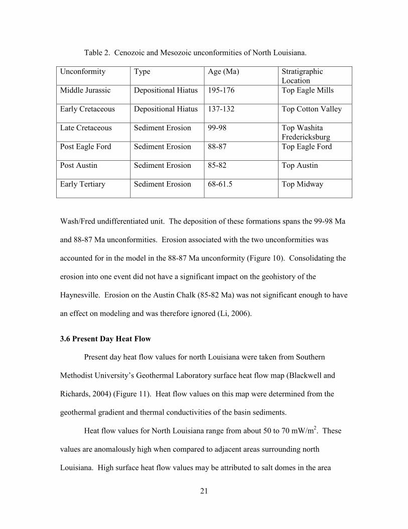
Table 2. Cenozoic and Mesozoic unconformities of North Louisiana.
Unconformity Type Age (Ma) Stratigraphic Location
Middle Jurassic Depositional Hiatus 195-176 Top Eagle Mills
Early Cretaceous Depositional Hiatus 137-132 Top Cotton Valley
Late Cretaceous Sediment Erosion 99-98 Top Washita Fredericksburg
Post Eagle Ford Sediment Erosion 88-87 Top Eagle Ford
Post Austin Sediment Erosion 85-82 Top Austin
Early Tertiary Sediment Erosion 68-61.5 Top Midway
Wash/Fred undifferentiated unit. The deposition of these formations spans the 99-98 Ma
and 88-87 Ma unconformities. Erosion associated with the two unconformities was
accounted for in the model in the 88-87 Ma unconformity (Figure 10). Consolidating the
erosion into one event did not have a significant impact on the geohistory of the
Haynesville. Erosion on the Austin Chalk (85-82 Ma) was not significant enough to have
an effect on modeling and was therefore ignored (Li, 2006).
3.6 Present Day Heat Flow Present day heat flow values for north Louisiana were taken from Southern
Methodist University’s Geothermal Laboratory surface heat flow map (Blackwell and
Richards, 2004) (Figure 11). Heat flow values on this map were determined from the
geothermal gradient and thermal conductivities of the basin sediments.
Heat flow values for North Louisiana range from about 50 to 70 mW/m2. These
values are anomalously high when compared to adjacent areas surrounding north
Louisiana. High surface heat flow values may be attributed to salt domes in the area

22
Figure 10. A) Eroded thickness (feet) of the missing Cretaceous section in north Louisiana from Li (2006). Well control is shown by red and blue dots (Li, 2006) B) locations of wells used by Li ( 2006).
A. B.
B.

Figure 11. North America heat flow map (Blackwell and Richards, 2004) and/or an increase of radioactive elements in the basement rocks. Salt has a thermal
conductivity on the order of 2 to 4 times greater than other sedimentary rocks (Gray and
Nunn, 2010). An average present day heat flow value of 60
study. Slight variations in present day heat flow
day %Ro values, but do not significantly impact the thermal history of the Haynesville
and timing of hydrocarbon generation.
3.7 Paleoheat Flow The North Louisiana Salt Basin formed as a result of rifting during the opening of
the Gulf of Mexico from the Late Triassic to Early Jurassic (
flow values associated with the opening of the basin were calculated
simple extensional model (McKenzie, 1978).
23
Figure 11. North America heat flow map (Blackwell and Richards, 2004)
ncrease of radioactive elements in the basement rocks. Salt has a thermal
conductivity on the order of 2 to 4 times greater than other sedimentary rocks (Gray and
An average present day heat flow value of 60 mW/m2 was used in this
Slight variations in present day heat flow result in negligible differences in present
Ro values, but do not significantly impact the thermal history of the Haynesville
and timing of hydrocarbon generation.
Louisiana Salt Basin formed as a result of rifting during the opening of
the Gulf of Mexico from the Late Triassic to Early Jurassic (Pilger, 1981). Paleoheat
associated with the opening of the basin were calculated in PetroMod
extensional model (McKenzie, 1978).
ncrease of radioactive elements in the basement rocks. Salt has a thermal
conductivity on the order of 2 to 4 times greater than other sedimentary rocks (Gray and
was used in this
result in negligible differences in present
Ro values, but do not significantly impact the thermal history of the Haynesville
Louisiana Salt Basin formed as a result of rifting during the opening of
Pilger, 1981). Paleoheat
in PetroMod using a

24
Paleoheat flow values calculated by the McKenzie model are impacted by rifting
and the amount of lithospheric extension. A rifting period from 190-170 mya was used.
Lithospheric extension is quantified using the beta factor (β), which is the ratio of
lithosphere thickness before and after extension. The beta factor for North Louisiana is
approximately 1.5-2 (Nunn et al., 1984). Paleoheat flow increased to a maximum at the
end of the rifting phase.
Two paleoheat flow models were used in this study. Paleoheat flows of
sediment overlying the Sabine and Monroe Uplifts were calculating using a beta factor of
1.5 (Figure 11) because it is inferred the crust there is less extended. Sediments
deposited in the North Louisiana Salt Basin are inferred to overlie more extended crust
and paleoheat flow values were calculated using a beta factor of 1.8 (Figure 12).
3.8 Thermal Maturity Thermal maturity of the Haynesville Shale was computed from the burial history
and thermal history using The EASY %Ro kinetic model (Burnham and Sweeny, 1989) in
PetroMod®. Observed TOC (total organic carbon) values in the Haynesville Shale
typically range from 2-6% (Dix et al., 2010) a value of 5% was used for modeling. TOC
weight percent is not an approximate estimation of resource present, and must be used
with caution when estimating the amount of hydrocarbons generated (Dembicki, 2009).
As the source rock generates and expels hydrocarbons, the amount of organic matter in
the source rock (TOC) and hydrogen index (HI) will decrease.

25
A)
B)
Figure 12. Paleo heat flow models used in this study. A) Calculated using a beta factor of 1.5 and used for wells located on the Sabine Uplift. B) Calculated using a beta factor of 1.8 and used for wells located in the deep basin and south of the Sabine Uplift.
3.9 Porosity and Pressure
Porosity estimates were calculated using the PetroMod® software. Porosity
estimates are based on Athy’s Law (1930) of mechanical sediment compaction.
Sediments progressively lose their porosity as a function of depth due to the effects of
loading. Athy used the following equation to estimate porosity:
Φ=Φ0 e(-az) (1)
Where Φ is estimated porosity, z = sub bottom depth (in meters), and Φ0 and a are
constants that vary with sediment type and burial history. Initial porosity of sediment
depends on lithology. Shales and mudstones start with porosities > 60%, sandstones
~40%, and carbonates can start as high as ~70% (Sclater and Christie, 1980). Fluid
pressures were computed as a function of overburden stress and fluid expansion in 1D
and 2D using PetroMod® software.

26
3.10 Paleowater Depths and Sediment Water Interface Temperature Paleowater depths and eustatic sea level correlations have not been
incorporated in this study because it is assumed that the sediments were deposited
in a shallow water environment (Nunn, 1984). The maximum estimated water
depth in north Louisiana in the Tertiary through the Jurassic is approximately 100
to 150 meters (Zimmerman, 1999). The effects of water loading at these depths are
believed to be negligible (Li, 2006).

27
Chapter 4. Results Models from four wells were chosen to display how burial, maturation, and
pressure history varies across the basin (Figure 13).
4.1 Thermal Maturation The transformation of kerogen to oil is interpreted to initiate at a vitrinite
reflectance (R0) value of 0.55%. The process of oil generation reaches completion at a
vitrinite reflectance value of 1%. The last liquid hydrocarbons are cracked to wet gas at
an R0 value of 1.3%. The shift from wet gas to dry gas occurs at an R0 value of 2.0%.
The production of dry gas ceases at an R0 value of 4.0% (Sweeney and Burnham, 1990).
The kerogen types associated with the Haynesville Shale were mainly gas prone type III
and some oil and gas prone type II/III (Mancini et al., 2008). Because oil generation
results in greater overpressure than gas generation, type II kerogen was used for all
models to simulate maximum pressures resulting from hydrocarbon generation. In the
North Louisiana Salt Basin, the Haynesville Shale began hydrocarbon generation in the
early Cretaceous and has continued into the Tertiary (Figure 14). On the Sabine Uplift,
calculated present day R0 values fall in the wet gas range. South and east of the Sabine
Uplift, Haynesville Shale maturity increases as depth of burial increases. R0 values fall
into the dry gas range.
1D basin models show that the earliest hydrocarbon generation within the
Haynesville Shale began in the deepest part of the basin and occurred at progressively
younger times for shallower beds (Figure 15). The onset of hydrocarbon generation
ranges from about 140-130 Ma in the study area. Modeled Haynesville R0 values range
from about 1.5% on the Sabine Uplift to 2.7% in the deep basin to 0.8% on the Monroe

28
Uplift (Appendix C). R0 values suggest the Haynesville has generated mostly gas.
Thermal maturity values are consistent with measured data (Mancini et al., 2008).
Figure 13. Map of study area showing the locations of the four wells discussed in the results and discussion sections. North to south cross section, A-A’, and west to east cross section, B-B; used in 2D models are shown in black.
4.2 Fluid Pressure In this study, 1D models were created to predict pore pressure as a function of
disequilibrium compaction and hydrocarbon generation. By definition 1D models do not
incorporate the effects of lateral fluid migration. Pore pressure, hydrostatic pressure,
lithostatic pressure, and the fracture pressure are plotted versus depth. The fracture
pressure computed in PetroMod® for all lithologies is 80% of the difference between the

29
A)
1-G
ish
(Sab
ine)
C
) 1-F
oste
r (Sa
bine
)
B)
C1-C
ates
(So
uth
of S
abin
e)
D)
C1-
Tre
mon
t (N
LSB
)
Figu
re 1
4. B
uria
l his
tory
plo
ts fr
om 1
D m
odel
s w
ith E
ASY
%R
O (S
wee
ny a
nd B
urnh
am, 1
990)
ove
rlay
for A
) 1-G
ish
(Sab
ine
Upl
ift)
, B
) 1-C
ates
(sou
th o
f Sab
ine
Upl
ift)
, C) 1
-Fos
ter (
Sabi
ne U
plif
t), a
nd D
) C1-
Tre
mon
t (ba
sin
cent
er) w
ells
.

30
Figure 15. Plot of vitrinite reflectance versus time from 1D models for the Haynesville Shale for four wells. The onset of hydrocarbon generation occurs at R0 = 0.55%, wet gas at R0 = 1.3%, and dry gas at R0 = 2% hydrostatic pressure and lithostatic pressure. 1D models show that the onset of present
day (0 Ma) overpressure begins in the Hosston Formation and increases with depth. 1D
models predict Haynesville overpressure to be greatest in areas of deep burial and for
pressure to decrease with burial depth (Figure 16). 1D modeling predicts the 1-Gish well
(Sabine Uplift) to have a present day pressure of 6,000 psi, the 1 Cates well (south of the
Sabine) 9,300 psi, 1-Foster (Sabine) 7,300 psi and the C1-Tremont well (deep basin) to
have a pressure of 11,100 psi. 1D models based on compaction disequilibrium and
hydrocarbon generation underestimate pressures observed on the Sabine Uplift (1-Gish
and 1-Foster wells) by an average of 1,000 psi (Figure 5).
Due to the underestimation of pressure resulting from 1D model calculations
compared to pressure data from well tests (Wang and Hammes, 2010) (Figure 5), 2D
basin models were created to study the effect of fluid migration on the occurrence of
overpressure in the Haynesville Shale (Figures 17 and 18). Two regional cross sections
Time [Ma]
Vitrinite Reflectance [%Ro]
Gish (Sabine)
Foster (Sabine)
Cates (south of Sabine)
Tremont (basin center)

31
were created from well data (Figure 13) to reflect the subsurface architecture of north
Louisiana. Two depth extractions were taken from each cross section at the well
locations: 1 Gish, 1 Cates, 1 Foster, and C1 Tremont (Figure 19). Extractions from the
2D model were used to compare the difference in pressure calculated using 1D and 2D
models. 2D pressure models predict present day (0 Ma) overpressure to begin at the top
of the Hosston Formation. 2D models A-A’ (Figure 17) and B-B’ (Figure 18) predict that
the greatest Haynesville Shale pore pressures are generated in the deep basin and pressure
progressively decreases as the depth to the Haynesville Shale decreases. In the north to
south cross section, A-A’ (Figure 17), estimated Haynesville Shale pore pressure ranges
from 9,000 psi south of the Sabine Uplift to 7,000 psi over the Sabine Uplift. South of
the Sabine Uplift a decrease in pressure relative to the overlying strata occurs in the lower
Bossier and Haynesville Formations. In the west to east cross section, B-B’ (Figure 18),
estimated Haynesville Shale pore pressures range from 10,000 in the deep basin to 8,200
on the Sabine Uplift. In the deepest part of the basin there is a decrease in pressure that
occurs in the lower Bossier and Haynesville relative to the overlying and underlying
strata. Haynesville Shale fluid pressure is nearest the fracture gradient on the Sabine
Uplift (Figure 20) directly after the Cretaceous reactivation of the Sabine Uplift and
erosion event occurring at 87 Ma (Figures 21 and 22)
4.3 Fluid Migration
Hydrocarbon flow path modeling shows that lateral fluid migration and vertical
migration into overburden and underburden formations has occurred in the Haynesville
Shale. In the north to south cross section model A-A’ (Figure 23), model results show
hydrocarbons generated in the Haynesville are expelled vertically into the overlying

32
A) 1 Gish at 0 Ma B) 1 Foster at 0
C) 1 Cates at 0 Ma D) C1 Tremont at 0 Ma
Figure 16. Pressure versus depth from 1D models. Modeled pressure estimates at the Haynesville Shale are as followed: a) 1 Gish - 6,000 psi, b) 1 Cates – 9,300 psi, c) 1 Foster – 7,000 psi, and d) C1 Tremont – 11,100 psi. Estimated pressure from well test data (Wang and Hammes, 2010) shown by the blue stars. C) and D) are outside the data used by Wang and Hammes (2010).
33
Fi
gure
17.
2D
cro
ss s
ectio
n, n
orth
to s
outh
, at 0
Ma
with
por
e pr
essu
re o
verl
ay.
The
loca
tions
of t
he 1
Cat
es a
nd 1
Gis
h w
ells
are
sh
own
in b
lack
.
1 G
ish
1 Ca
tes
Nor
th
Sout
h
Hor
izon
tal g
rid
poin
ts

34
Fi
gure
18.
2D
cro
ss s
ectio
n, e
ast t
o w
est,
at 0
Ma
with
por
e pr
essu
re o
verl
ay.
The
loca
tions
of t
he 1
Fos
ter a
nd C
1 T
rem
ont w
ells
are
sh
own
in b
lack
.
1 Fo
ster
C1 T
rem
ont
Wes
t Ea
st
Hor
izon
tal g
rid
poin
ts

35
1 Gish at 0 Ma 1 Foster at 0 Ma
1 Cates at 0 Ma C1 Tremont at 0 Ma
Figure 19. Pressure at 0 Ma from 2D model at well locations. Pressures at the well locations are as follows: a) 1Gish – 6,900 psi b) 1 Foster – 8,200 c) 1 Cates – 8,400 psi and d) C1 Tremont – 10,000 psi. Estimated pressure from well test data (Wang and Hammes, 2010) shown by the blue stars.

36
1-Gish (Sabine)
1-Cates (South of Sabine)
1-Foster (Sabine)
C1-Tremont (deep basin)
Figure 20. Pore pressure and fracture pressure versus time. Extractions from 2D models at well locations. Pressures from wells located on the Sabine Uplift (1 Gish and 1 Foster) are nearest the fracture gradient at 87 Ma
Time [Ma]
Time [Ma]
Time [Ma]
Time [Ma]
Fracture Pressure
Pore Pressure
Fracture Pressure
Pore Pressure
Fracture Pressure
Pore Pressure
Fracture Pressure
Pore Pressure
150 100 50 0
150 100 50 0
150 100 50 0
150 100 50 0

37
Fi
gure
21.
2D
cro
ss s
ectio
n, n
orth
to s
outh
, at 8
7 M
a w
ith p
ore
pres
sure
ove
rlay
.
Nor
th
Sout
h
1 G
ish
1 Ca
tes
Hor
izon
tal g
rid
poin
ts

38
Fi
gure
22.
2D
cro
ss s
ectio
n, w
est t
o ea
st, a
t 87
Ma
with
por
e pr
essu
re o
verl
ay.
Wes
t Ea
st
1 Fo
ster
C1 T
rem
ont
Hor
izon
tal g
rid
poin
ts

39
Figu
re 2
3. 2
D c
ross
sec
tion,
nor
th to
sou
th, a
t 0 M
a w
ith p
ore
pres
sure
ove
rlay
. H
ayne
svill
e Sh
ale
gas
flow
pat
hs a
re in
dica
ted
by re
d ar
row
s an
d oi
l flo
w p
aths
are
indi
cate
d by
gre
en a
rrow
s.
Nor
th
Sout
h
1 G
ish
1 Ca
tes
Hor
izon
tal g
rid
poin
ts

40
Bossier Formation and the underlying Smackover Formation. Hydrocarbons generated
south of the Sabine are expelled downward into the more permeable Smackover
Formation and migrate updip along the Haynesville/Smackover interface toward the
Sabine Uplift. In the west to east cross section B-B’ (Figure 24), model results show
hydrocarbons generated in the deep basin migrate downward into the Smackover
Formation and then migrate updip along the Haynesville/Smackover interface to the
Sabine and Monroe Uplifts.
Similar hydrocarbon migration flow paths are observed at 87 Ma (Figures 25 and
26). In the deep basin or south of the Sabine, fluids are expulsed downward into the
Smackover formation and travel updip along the Haynesville/Smackover interface toward
the Sabine and Monroe Uplifts. Some lateral fluid migration occurs within the
Haynesville, but this model does not incorporate a possible increase in effective
permeability due to the propagation of natural hydraulic fractures which could greatly
enhance lateral fluid migration within the Haynesville Shale. Fluids are also expulsed
vertically into overlying formations at this time.
Water migration pathways are shown for the north to south cross section and the
west to east cross section (Figures 27 and 28). At 0 Ma and 87 Ma water from the
Haynesville Shale is expelled upward into overlying formations at the Sabine Uplift. Off
structure, water is expelled vertically into the underlying Smackover Formation. At 0 Ma
all water in the Smackover is migrating from south to north and east to west. At 87 Ma,
and throughout most of the basin history, water migrated updip toward the Sabine and
Monroe uplifts.

41
Figu
re 2
4. 2
D c
ross
sec
tion,
wes
t to
east
, at 0
Ma
with
por
e pr
essu
re o
verl
ay.
Hay
nesv
ille
Shal
e ga
s fl
ow p
aths
are
indi
cate
d by
red
arro
ws
and
oil f
low
pat
hs a
re in
dica
ted
by g
reen
arr
ows.
Wes
t Ea
st
1 Fo
ster
C1 T
rem
ont
Hor
izon
tal g
rid
poin
ts

42
Figu
re 2
5. 2
D c
ross
sec
tion,
nor
th to
sou
th, a
t 87
Ma
with
por
e pr
essu
re o
verl
ay.
Hay
nesv
ille
Shal
e ga
s fl
ow p
aths
are
indi
cate
d by
re
d ar
row
s an
d oi
l flo
w p
aths
are
indi
cate
d by
gre
en a
rrow
s.
Nor
th
Sout
h
1 G
ish
1 Ca
tes
Hor
izon
tal g
rid
poin
ts
43
Figu
re 2
6. 2
D c
ross
sec
tion,
wes
t to
east
, at 8
7 M
a w
ith p
ore
pres
sure
ove
rlay
. H
ayne
svill
e Sh
ale
gas
flow
pat
hs a
re in
dica
ted
by re
d ar
row
s an
d oi
l flo
w p
aths
are
indi
cate
d by
gre
en a
rrow
s.
Wes
t Ea
st
1 Fo
ster
C1 T
rem
ont
Hor
izon
tal g
rid
poin
ts

44
Figure 27. 2D cross sections, north to south and west to east, at 0 Ma with vertical permeability overlay. Water flow paths are represented by blue arrows.
North South
0 Ma West
0 Ma
1 Gish
1 Cates
1 Foster
East
C1 Tremont
Horizontal grid points
Horizontal grid points
45
Figure 28. 2D cross sections from north to south and west to east at 87 Ma with vertical permeability overlay. Water flow paths are represented by blue arrows.
1 Gish
1 Cates
1 Foster
C1 Tremont
87 Ma North South
West 87 Ma
East
Horizontal grid points
Horizontal grid points
46
Chapter 5. Discussion
5.1 Sensitivity Studies Thermal maturation of the Hayneville Shale resulted in the onset of hydrocarbon
generation in the early Cretaceous. 1D and 2D models run with and without the effects
of hydrocarbon generation produced nearly identical results for present day pore pressure
indicating that much of the pressure resulting from hydrocarbon generation has dissipated
over time. Previous numerical modeling studies have shown that although hydrocarbon
generation contributes to overpressure, disequilibrium compaction is the most important
mechanism (Chi et al., 2010). Hydrocarbon generation plays an important role in the
pressure history of the Haynesville Shale. Hydrocarbon generation may result in an
increase in pressure (hydrocarbon generation pressure) due to the conversion of high
density kerogen into low density hydrocarbons. 2D model results show hydrocarbon
generation pressure maximums occurring in the late Cretaceous between 105-85 Ma
(Figure 29) with hydrocarbon generation pressure greatest just prior to Cretaceous uplift
and erosion at 88 Ma. Hydrocarbon generation pressure nears 500 psi at 88 Ma south of
the Sabine Uplift near the 1-Cates well (Figures 30 and 31). On the Sabine Uplift
hydrocarbon generation pressure at the 1-Gish well reaches a maximum of 60 psi (Figure
29). Due to the dynamic nature of fluids and the relatively thin stratigraphy of the
Haynesville Shale, large pressure increases due to hydrocarbon generation observed
south of the Sabine Uplift are not sustained over geologic time. Modeled hydrocarbon
generation pressures from 1D calculations are at least one order of magnitude lower than
hydrocarbon generation pressures calculated from 2D models. Haynesville Shale
overpressures resulting from disequilibrium compaction alone are at least one to two

47
orders of magnitude greater than the largest pressure increases due to hydrocarbon
generation.
Haynesville Shale Hydrocarbon Generation Pressure 1-Gish
Haynesville Shale Hydrocarbon Generation Pressure 1-Cates
Figure 30. Haynesville Shale hydrocarbon generation pressure versus time extracted from 2D model at the 1-Gish well (Sabine) and 1-Cates well (south of Sabine). Peaks in pressure occur from 105 – 85 Ma.

48
Figure 30. Pressure increases due to Haynesville Shale hydrocarbon generation in the north to south cross-section at 105 and 88 Ma. Haynesville Shale hydrocarbon generation pressure reaches a maxium at 88 Ma.
1 Gish
1 Cates
North South Hydrocabon Generation Pressure– 105 Ma
North South
1 Gish
1 Cates
Hydrocabon Generation Pressure– 88 Ma
Horizontal grid points
Horizontal grid points

49
Figure 31. Pressure increases due to Haynesville Shale hydrocarbon generation in the north to south cross-section at 87 and 85 Ma.
North South
North South
1 Gish
1 Cates
1 Gish
1 Cates
Hydrocarbon Generation Pressure– 87 Ma
Hydrocarbon Generation Pressure– 85 Ma
Horizontal grid points
Horizontal grid points

50
Fluid overpressure related to disequilibrium compaction is sensitive to rock
permeability and permeability values for a given lithology can vary over several orders of
magnitude. Simulations for fluid pressure were carried out varying the permeability of
the Hosston, Cotton Valley, and Bossier Formations by one and two orders of magnitude
lower than the PetroMod® software default permeability for the Shale (sandy) lithology.
PetroMod® assigns permeability based a multipoint porosity/permeability model. Each
point in this model is assigned porosity and permeability value. Each permeability value
at a given porosity was decreased by either one or two orders of magnitude during this
sensitivity study. Fluid overpressure increased significantly with decreasing permeability
as shown from the pressure profile from the 1-Gish well (Sabine Uplift) (Figure 33).
Varying the permeability in these formations also has an effect on the porosity and
permeability development of the Haynesville Shale and Smackover Limestone (Figure
34). Lowering the permeability of the Hosston, Cotton Valley, and Bossier Formations
by one order of magnitude resulted in porosity and permeability values for these
formations and the Haynesville that are consist with values published from literature
(Mancini et al., 2008). Lowering the permeability of these formations by one order of
magnitude results in a 900 psi pressure increase for the 1 Gish well (1D calculation).
Rock permeability has an effect on fluid flow pathways. 2D models were run
varying the permeability of the Smackover Limestone by 1 and 2 orders of magnitude
lower than the default permeability for limestone (micrite) lithology. Using default
permeability, hydrocarbons expelled into the Smackover migrate updip along the
Haynesville/Smackover interface and reenter the Haynesville at the Sabine Uplift (Figure
23). If the Smackover permeability is decreased by 1 order of magnitude, hydrocarbons

51
continue to migrate downward into the Smackover Formation and laterally along the
Smackover/Haynesville interface.
Figure 32. 1D present day pore pressure versus depth profile for the 1 Gish well with variable permeabilities for the Hosston, Cotton Valley, and Bossier Formations. The red line represents pressure using a default PetroMod® permeability, the black line represents a one order of magnitude permeability decrease, and the purple line represents a 2 order of magnitude permeability decrease. The blue star represents pressure estimated from well test data (Wang and Hammes, 2010).
52
Figure 33. Present day A) porosity and B) permeability versus depth profiles for 1 Gish well at 0 Ma. The permeability of the Hosston, Cotton Valley, and Bossier Formations vary by one and two orders of magnitude.
A.
B.

53
The change in permeability does not significantly alter the pore pressure across the basin
(Figure 34). When the Smackover permeability was decreased by two orders of
magnitude downward hydrocarbon migration from the Haynesville Shale in the deep
basin continues, and hydrocarbons continue to migrate laterally along the
Haynesville/Smackover interface. The distribution of fluid pressure across the basin is
not significantly altered (Figure 34). The permeability of the Smackover must be
decreased much more significantly to have a profound impact on hydrocarbon migration
pathways through the Smackover.
The pre-erosional thicknesses of early Eocene sediment on the Sabine Uplift are
unknown. Facies distributions indicate the Sabine may have been subaerially exposed
during Eocene deposition (Jackson and Laubach, 1988; Laubach and Jackson, 1990).
Eocene erosion is not believed to have occurred on the Sabine Uplift and was not
accounted for in previous modeling studies (Li, 2006; Mancini et al., 2008). However, if
Eocene sediments were in fact deposited and eroded it could impact the pressure history
of the Haynesville Shale. Sensitivity analyses were run varying the magnitude of Eocene
erosion by 0 ft, 500 ft, and 1500 ft (Figure 36). 500 ft of Eocene deposition and
subsequent erosion increases present day Haynesville pore pressure at the 1 Gish well by
200 psi. 1500 ft of Eocene deposition and subsequent erosion increases present day
Haynesville pore pressure at the 1 Gish well by 800 psi. Results show that Eocene
erosion would have an effect on the pressure history of the Haynesville, but erosion on
the scale of thousands of feet would be needed to have a significant impact on the present
day pressure. It is unlikely Eocene erosion of that magnitude occurred on the Sabine
Uplift

54
Fi
gure
34.
Cro
ss s
ectio
n B
-B’ w
ith p
ore
pres
sure
ove
rlay
at 0
Ma.
Red
(ga
s) a
nd g
reen
(oil)
arr
ows
indi
cate
hyd
roca
rbon
flow
pa
thw
ays.
Sm
acko
ver L
imes
tone
per
mea
bilit
y va
lues
are
1 o
rder
of m
agni
tude
less
thos
e us
ed in
the
fina
l mod
el.
Wes
t Ea
st
1 Fo
ster
C1 T
rem
ont
Hor
izon
tal g
rid
poin
ts

55
Fi
gure
35.
Cro
ss s
ectio
n B
-B’ w
ith p
ore
pres
sure
ove
rlay
. R
ed (g
as) a
nd g
reen
(oil)
arr
ows
indi
cate
hyd
roca
rbon
flow
pat
hway
s.
Smac
kove
r Lim
esto
ne p
erm
eabi
lity
valu
es a
re 2
ord
ers
of m
agni
tude
less
thos
e us
ed in
the
fina
l mod
el.
Wes
t Ea
st
1 Fo
ster
C1 T
rem
ont
Hor
izon
tal g
rid
poin
ts

56
Figure 36. Pressure versus depth for 1 Gish D well at 0 Ma with varied amounts of Eocene erosion. (Jackson and Laubach, 1988; Laubach and Jackson, 1990).
The focus of this study is the Haynesville Shale. However, the Smackover
Formation is the major petroleum source rock in the North Louisiana Salt Basin (Sassen
et al., 1987; Mancini et al., 2005). The Smackover Limestone has a measured present-

57
day TOC average of 0.58% and a calculated original TOC average of 1.00% (Mancini et
al, 2005). The kerogen found in the Smackover is type I and the majority of
hydrocarbons generated are believed to have been expelled into younger formations
(Mancini et al., 2005). A model was run with Smackover hydrocarbon generation along
with Haynesville generation to test the impact of Smackover hydrocarbon generation on
the pressure history of the Haynesville. Smackover hydrocarbon generation resulted in
maximum overpressure of 1900 psi occurring in the upper Smackover at 88 Ma (Figures
38 and 39). The incorporation of Smackover hydrocarbon generation into the model does
not significantly alter the pressure history of the Haynesville Shale nor did it result in
overpressures great enough to hydraulically fracture the Haynesville at any point in time.
Hydrocarbons generated in the Smackover Formation migrate updip towards the Sabine
and Monroe Uplift.
5.2 Fluid Pressure Transfer
The effect of lateral fluid pressure transfer is observed by comparison of 1D and
2D models. In the N-S profile the 1 Gish well, located on the Sabine Uplift, shows an
increase of 1000 psi when migration is incorporated into the model (Figure 39). South
of the Sabine Uplift, the 1 Cates well shows a decrease in pressure in the Bossier Shale,
Haynesville Shale, and Smackover Limestone when fluid migration is applied to the
model. In the 2D model Haynesville Shale pore pressure decreases by 900 psi relative to
the 1D model (Figure 40). In the E-W profile, the 2D 1-Foster well, located on the
Sabine Uplift, shows an increase of 1200 psi relative to the 1D model (Figure 41). East
of the Sabine Uplift, in the deep basin, the 2D C1 Tremont well model shows a decrease
in pressure in the Bossier Shale, Haynesville Shale, and Smackover Limestone relative to

58
Figure 37. North to south 2D model showing Smackover and Haynesville hydrocarbon generation pressures at 105 and 88 Ma.
North South Generation Pressure– 105 Ma
North Generation Pressure– 88 Ma
1 Gish
1 Cates
1 Gish
1 Cates
Horizontal grid points
Horizontal grid points

59
Figure 38. North to south 2D model showing Smackover and Haynesville hydrocarbon generation pressures at 105 and 88 Ma.
1 Gish
1 Cates
1 Gish
1 Cates
Generation Pressure– 87 Ma North South
North South Generation Pressure– 85 Ma
Horizontal grid points
Horizontal grid points

60
1D model. Haynesville pore pressure decreases by 1300 psi (Figure 42). The increase in
pressure observed on the Sabine Uplift and decrease in pressure in the deep basin in the
2D models relative to the 1D models is evidence that lateral fluid pressure transfer has
occurred within the Haynesville Shale and underlying Smackover Formation.
2D fluid migration modeling indicates that lateral fluid pressure transfer is largely
influenced by burial depth. Overpressures increase as depth of burial increases. Fluids
migrate from areas of deep burial and high overpressure to structural highs. Therefore
fluid pressure transfer occurring at 0 Ma is strongly influenced by the present day
structure of the basin. The top of the Smackover Formation was contoured to estimate
basin wide fluid migration at 0 Ma (Figure 43).
5.3 Hydrocarbon Migration
The direction of hydrocarbon migration is dependent on the pressure gradient,
permeability of the strata, capillary effects, and buoyancy force (Hubbert, 1953). The
model results indicate that the maximum occurrence of overpressure in the Haynesville
Shale occurs where depth of burial is the greatest. In the central basin of the west to east
cross section an increase in fluid pressure relative to the Haynesville Shale occurs in the
overlying Bossier Shale, forming a pressure barrier for upward fluid migration (Figure
24). The variations in fluid pressures in the deep basin resulted in a pressure gradient
favorable for the downward migration of fluid into the Smackover Limestone. Once
fluids were expelled into the underlying Smackover Limestone, the fluids migrate
laterally updip toward structural highs.
2D basin models predict that the Haynesville Shale pressure was nearest the
fracture gradient directly following the Cretaceous reactivation of the Sabine Uplift at 87

61
B) 1 Gish 2D
B) 1 Cates 2D
Figure 39. A) Present day pore pressure at 1 Gish well estimated from 1D model – 6,000 psi and B) pore pressure at 1 Gish well estimated from 2D model – 6,900 psi. The blue stars show pore pressure estimated from well test data (Wang and Hammes, 2010).
Figure 40. A) Present day pore pressure at 1 Cates well estimated from 1D model – 9,300 psi and B) pore pressure at 1 Gish well estimated from 2D model – 8,400 psi.
A) 1 Gish 1D
A) 1 Cates 1D

62
B) 1 Foster 2D
B) C1 Tremont 2D
Figure 41. A) Present day pore pressure at 1 Foster well estimated from 1D model – 7,000 psi and B) pore pressure at 1 Gish well estimated from 2D model – 8,200 psi. The blue stars show pore pressure estimated from well test data (Wang and Hammes, 2010)
Figure 42. A) Present day pore pressure at C1 Tremont well estimated from 1D model – 11,000 psi and B) pore pressure at C1 Tremont well estimated from 2D model – 10,000 psi.
A) 1 Foster 1D
A) C1 Tremont 1D
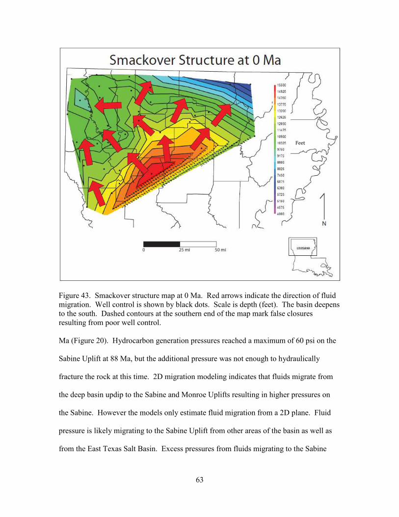
63
Figure 43. Smackover structure map at 0 Ma. Red arrows indicate the direction of fluid migration. Well control is shown by black dots. Scale is depth (feet). The basin deepens to the south. Dashed contours at the southern end of the map mark false closures resulting from poor well control. Ma (Figure 20). Hydrocarbon generation pressures reached a maximum of 60 psi on the
Sabine Uplift at 88 Ma, but the additional pressure was not enough to hydraulically
fracture the rock at this time. 2D migration modeling indicates that fluids migrate from
the deep basin updip to the Sabine and Monroe Uplifts resulting in higher pressures on
the Sabine. However the models only estimate fluid migration from a 2D plane. Fluid
pressure is likely migrating to the Sabine Uplift from other areas of the basin as well as
from the East Texas Salt Basin. Excess pressures from fluids migrating to the Sabine
Feet

64
may result in overpressures great enough to hydraulically fracture the Haynesville Shale
at 87 Ma (Figure 20).
5.4 Natural Hydraulic Fractures
Anisotropy due to natural fractures in the Haynesville was not accounted for in
this study but likely has an influence on hydrocarbon flow pathways. Lateral fluid
migration may have been facilitated through increased permeability along bedding planes
and natural hydraulic fractures. The propagation of natural hydraulic fractures would
increase the effective permeability of the Haynesville Shale and aid lateral fluid
migration. Haynesville Shale overpressure was closest to the fracture gradient on the
Sabine Uplift directly following the Cretaceous erosional event at 87 Ma. 2D models
show fluid migration occurring from the deep basin to the Sabine Uplift. A 3D model is
needed to incorporate fluid migration from the North Louisiana Salt Basin and East
Texas Salt Basin to the Sabine Uplift. 2D modeling suggests that at 87 Ma Haynesville
Shale overpressure was very near the fracture gradient. It is likely that 3D focusing of
fluid flow to structural highs would predict overpressures in excess of the fracture
gradient at this time. This would greatly enhance the effective permeability of the
Haynesville and fluid flow at this time. In order to estimate fluid migration pathways at
87 Ma 39 wells were decompacted and the top of the Smackover at 87 Ma was mapped
across the North Louisiana Salt Basin (Figure 44). 2D pressure models indicate that
Haynesville Shale fluids migrate from the deep basin towards the Sabine and Monroe
Uplifts. The propagation of natural hydraulic fractures during this time may have aided
fluid migration.

65
The Haynesville Shale is characterized by low permeability on the nanodarcy
scale (Wang and Hammes, 2010). Natural fractures can play a role in increasing the
permeability of this otherwise tight rock. Little research has been made public on
Haynesville Shale fractures, therefore the role of hydraulic fractures in fluid migration
within the Haynesville Shale is poorly understood. However, natural fractures are
common in petroleum source rocks (Gale et al., 2007; Engelder et al., 2009) and have
been observed in the Haynesville Shale (Buller and Dix, 2009). Most natural fractures in
the Haynesville have been mineralogically healed evidencing paleo fluid flow.
Horizontal hydraulic fractures may have increased the effective permeability and aided
the lateral migration of fluid pressure within the Haynesville Shale. Horizontal hydraulic
fractures may connect with joints or faults to aid expulsion of fluid pressure into
overlying and underlying formations. Hydrocarbon generation causes a localized
pressure increase within the Haynesville allowing fluids to be expulsed vertically into
overlying and underlying formations. Fluids expulsed into the underlying, more
permeable Smackover Limestone migrate laterally updip. On the Sabine Uplift, fluid
pressures increase within the Haynesville and Smackover due to lateral fluid pressure
transfer.
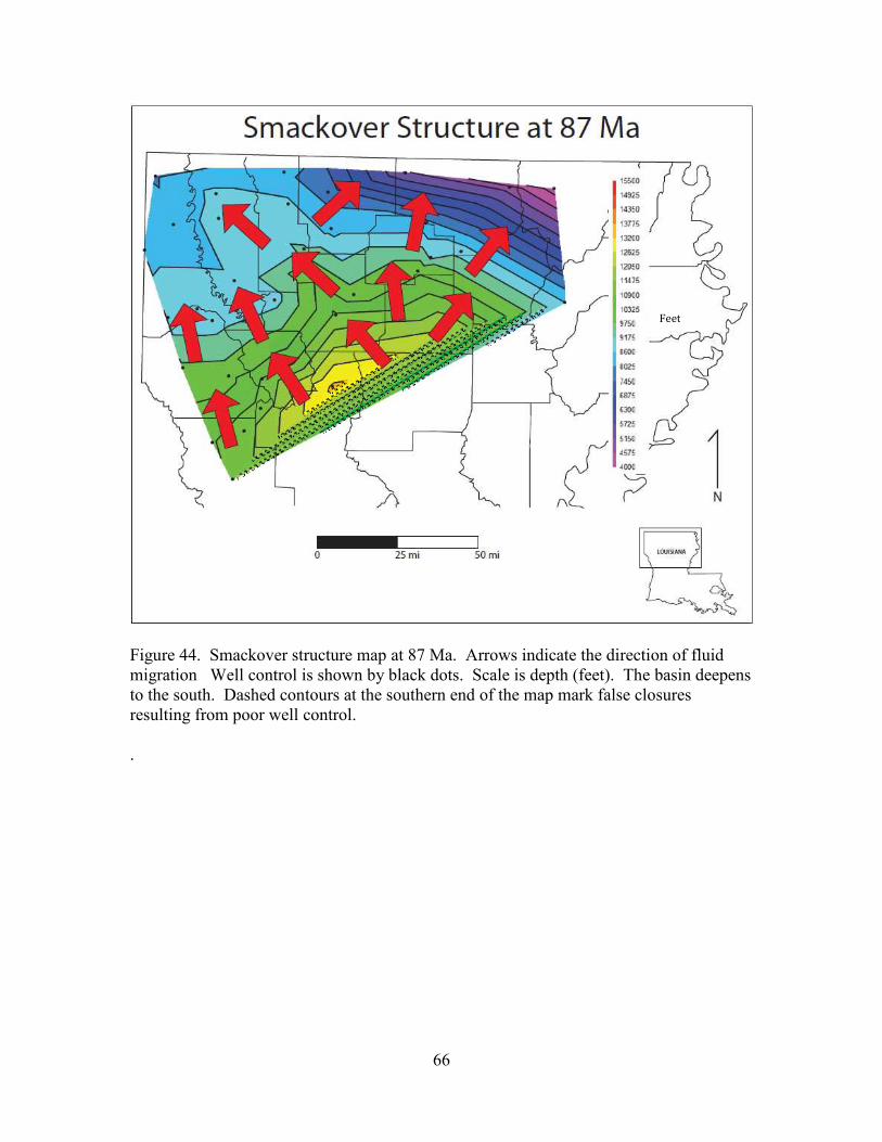
66
Figure 44. Smackover structure map at 87 Ma. Arrows indicate the direction of fluid migration Well control is shown by black dots. Scale is depth (feet). The basin deepens to the south. Dashed contours at the southern end of the map mark false closures resulting from poor well control. .
Feet

67
Chapter 6. Conclusions 1D and 2D basin models were created to estimate the burial history, thermal
history, and pressure history of the Haynesville Shale. Disequilibrium compaction
coupled with hydrocarbon generation has resulted in significant overpressures within the
Haynesville Shale. However disequilibrium compaction is the main control over the
occurrence of overpressure as hydrocarbon generation in the Haynesville resulted in a
maximum pressure increase of 500 psi compared to compaction disequilibrium results.
1D pore pressure models underestimate pore pressures calculated from well test data
from wells located on the Sabine Uplift (Wang and Hammes, 2010) by an average of
2000 psi. 2D pore pressure models underestimate well test data from wells located on the
Sabine Uplift by an average of 500 psi. Results from 2D models show higher pore
pressure on the Sabine Uplift compared to 1D model, and lower pressures in the deep
basin compared to 1D models, thus indicating that lateral fluid pressure transfer plays a
significant role in distribution of Haynesville fluid pressure. Hydrocarbon and water
migration modeling show that fluids expelled from the Haynesville Shale into the
underlying Smackover Formation migrate laterally updip along the
Haynesville/Smackover interface towards the Sabine and Monroe Uplifts. 1D and 2D
models did not produce Haynesville pore pressures in excess of the fracture gradient.
However, 2D Haynesville pressure models were very near the fracture gradient on the
Sabine Uplift following the Cretaceous erosion event due to a decrease in overburden
stress coupled with maximum hydrocarbon generation pressures. A 3D fluid migration
model that incorporates the entire North Louisiana Salt Basin and the East Texas Salt
Basin are needed to accurately estimate the pressure history of the Haynesville Shale on

68
the Sabine Uplift. Natural hydraulic fractures would increase the effective lateral
permeability of the Haynesville Shale and aid fluid migration toward the Sabine Uplift.
69
References Athy, L. F., 1930, Density, porosity, and compaction of sedimentary rocks: The
American Association of Petroleum Geologists Bulletin, v. 14, p. 1-21. Blackwell, D. D., and M. Richards, 2004, Geothermal Map of North America: American
Association of Petroleum Geologists, scale 1:6,500,000.
Buller, D., and M. C. Dix, 2009, Petrophysical evaluation of the Haynesville Shale in northwest Louisiana and northeast Texas: Gulf Coast Geological Association of Geological Societies Transactions, v. 59, p. 127-143.
Burnham, A. K., and J. J. Sweeney, 1990, Evaluation of a simple model of vitrinite reflectance based on chemical kinetics: The American Association of Petroleum Geologists Bulletin, v. 74, No. 10, p. 1559-1570.
Cobbold, P. R. and N. Rodrigues, 2007, Seepage forces, important factors in the formation of horizontal hydraulic fractures and bedding-parallel fibrous veins ('beef' and 'cone-in-cone'): Geofluids, v. 7, p. 313-322.
Chi, G. X., D. Lavoie, R. Bertrand, and M. K. Lee, 2010. Downward hydrocarbon
migration predicted from numerical modeling of fluid overpressure in the Paleozoic Anticosti Basin, eastern Canada: Geofluids, v. 10, p. 334-350.
Christopher, R. A., 1982, Palynostratigraphy of the basal Cretaceous units of the eastern Gulf and southern Atlantic coastal plains: in D. D. Arden, B. F. Beck, and E. Morrow, eds., Proceedings of the Second Symposium on the Geology of the Southeastern Coastal Plain: Georgia Geological Survey Information Circular, v. 53, p. 10-23.
Dembicki, H. Jr., 2009, Three common source rock evaluation errors made by geologists during prospect or play appraisals: American Association of Petroleum Geologists Bulletin, v. 93, p. 341-356.
Engelder, T., G. G. Lash, and R. S. Uzacategui, 2009, Joint sets that enhance production from Middle and Upper Devonian gas shales of the Appalachian Basin: American Association of Petroleum Geologists Bulletin, v. 93, p. 857-899.
Ewing, T. E., 2001, Review of Late Jurassic depositional systems and potential hydrocarbon plays, northern Gulf of Mexico Basin: Gulf Coast Geological Association of Geological Societies Transactions, v. 51, p. 85-96. Ewing, T. E., 2009, The ups and downs of the Sabine Uplift and the Northern Gulf of Mexico Basin: Jurassic basement blocks, Cretaceous thermal uplifts, and Cenozoic flexure: Gulf Coast Association of Geological Societies Transactions, v. 59, p. 253-269.

70
Fan, L., J.W. Thompson, and J. R. Robinson, 2010, Understanding gas production
mechanisms and effectiveness of well stimulation in the Haynesville Shale through reservoir simulation: Paper CSUG/SPE 136696 presented at the Canadian Unconventional Resources and International Petroleum Conference, Calgary, 9-21 October.
Gale, J. F., R. M. Reed, and J. Holder, 2007, Natural fractures in the Barnett Shale and their importance for hydraulic fracture treatments: American Association of Petroleum Geologists Bulletin, v. 91, p. 603-622.
Goldhammer, R. K., 1998, Second-order accommodation cycles and points of
“stratigraphic turnaround”: Implications for carbonate buildup reservoirs in Mesozoic carbonate systems of the East Texas Salt Basin, and south Texas, in W. D. Demis and M. K. Nelis, eds, West Texas Geological Society Annual Field Conference Guidebook, West Texas Geologic Society Publication 98-105, p. 11-28.
Geologic Consulting Services, 1976, Type Log: Tertiary and Mesozoic N. LA & S.
ARK. Houston, TX. Gray, T. A., and J. A. Nunn, 2010, Geothermal Resource Assessment of the Gueydan Salt
Dome and the Adjacent Southeast Gueydan Field, Vermillion Parish, Louisiana: Gulf Coast Association of Geological Societies Transactions, v. 60, p. 307-323.
Guo, X., S. He, K. Liu, and L. Zheng, 2011, Quantitative estimation of overpressure
caused by oil generation in petroliferous basins: Organic Geochemistry, v. 42, p. 1343-1350.
Hammes, U., H. S. Hamlin, and T. E. Ewing, 2011, Geologic analysis of the Upper
Jurassic Haynesville Shale in east Texas and west Louisiana. The American Association of Petroleum Geologists, v. 95, No. 10, p. 1643-1666.
Hantschel, T., and A. I. Kauerauf, 2010, Fundamentals of Basin and Petroleum Systems Modeling. Springer-Vertag, Berlin, Heidelberg, p. 1-29. Hubbert, M. K., 1953, Entrapment of petroleum under hydrodynamic conditions: American Association of Petroleum Geologists Bulletin, v. 37, p. 1956 - 2026. Hubbert M. K., W. D. Will, 1957, Mechanics of hydraulic fracturing. Petroleum
Transactions of the American Institute of Mining Engineers, v. 210, p. 153-168.
Hunt, J. M., 1990, Generation and migration of petroleum from abnormally pressured fluid compartments: American Association of Petroleum Geologists Bulletin, v. 74, p. 1-12.

71
Imlay, R. W., 1940, Lower Cretaceous and Jurassic formations of southern Arkansas and their oil and gas possibilities: Arkansas Division of Geology Information Circular, v. 12, p. 1-64.
Imlay, R. W., and G. Herman, 1984, Upper Jurassic ammonites of the subsurface
of Texas, Louisiana, and Mississippi: in W. P. S. Ventress, D. G. Bebout, B. F. Perkins, and C. H. Moore, eds., The Jurassic of the Gulf Rim: Proceedings of the Third Annual Research Conference, Gulf Coast Section, Society of Economic Paleontologists and Mineralogists Foundation, p. 149-170.
Jackson, M. L. W., and S. E. Laubach, 1988, Cretaceous and Tertiary compressive tectonics as the cause of the Sabine Arch, east Texas and northeast Louisiana: Gulf Coast Association of Geological Societies Transactions, v. 38, p. 245-256.
Laubach, S. E., and M. L. W. Jackson, 1990, Origin of arches in the northwestern Gulf of Mexico Basin: Geology, v. 18, p. 595-598.
Li, Peng, 2006, Modeling of Thermal Maturity of Strata in the North Louisiana Salt
Basin Area: Gulf Coast Association of Geological Societies Transactions, v. 56, p. 439-454.
Lou, X., and G. Vasseur, 1992, Contributions of compaction and aquathermal pressuring to geopressure and the influence of environmental conditions: American Association of Petroleum Geologists Bulletin, v. 76, p. 1550-1559.
Mancini, E. A., L. Peng, D. A. Goddard, V. Ramirez, and S. C. Talukdar, 2008, Mesozoic
(Upper Jurassic-Lower Cretaceous) deep gas reservoir play, central and eastern Gulf coastal plain: American Association of Petroleum Geologists Bulletin, v. 92, p. 283-308.
Mancini, E. A., T. M. Puckett, and B. H. Tew, 1996, Integrated biostratigraphic
and sequence stratigraphic framework for Upper Cretaceous strata of the eastern Gulf Coastal Plain, USA: Cretaceous Research, v. 17, p. 645-669.
Mancini, E. A., and J. W. Payton, 1981, Petroleum geology of South Carlton Field,
Lower Tuscaloosa “Pilot Sand”, Clarke and Baldwin counties, Alabama: Gulf Coast Association of Geological Societies Transactions, v. 31, p. 139- 147.
Mancini, E. A., and B. H. Tew, 1991, Relationships of Paleogene stage and planktonic foraminiferal zone boundaries to lithostratigraphic and allostratigraphic contacts in the eastern Gulf Coastal Plain: Journal of Foraminiferal Research, v. 21, p. 48-66.

72
Mancini, E. A., P. Li, D. A. Goddard, and R. K. Zimmerman, 2005, Petroleum source rocks of the onshore interior salt basins, north central and northeastern Gulf of Mexico: Gulf Coast Association of Geological Transactions, v. 55, p. 486 – 504.
Mandl, G., R. M. Harkness, 1987, Hydrocarbon migration by hydraulic fracturing. In:
Deformation of sediments and sedimentary rocks. Ed. Jones M. E., and R. M. F Preston, Geological Society of London Special Publications, 29, 39-53.
Mickus, K. L., and G. R. Keller, 1992, Lithospheric structure of the south-central United States: Geology, v. 20, p 387-390, doi: 10.1120/G25465A.1.
Nunn, J. A., 1996, Buoyancy-driven propagation of isolated fluid-filled fractures:
Implications for fluid transport in Gulf of Mexico geopressured sediments: Journal of Geophysical Research, v. 101, no. B2, p. 2963-2970.
Nunn, J. A., 1990, Relaxation of Continental Lithosphere: An Explanation For Late Cretaceous Reactivation of the Sabine Uplift of Louisiana-Texas: Tectonics, v. 9, no. 2, p. 341-359.
Nunn, J. A., A. D. Scardina, R. H. Pilger Jr., 1984, Thermal Evolution of the North-
Central Gulf Coast: Tectonics: v. 3, no. 7, p. 723-740. Peters, K. E., L. B. Magoon., C. Lampe, A. H. Scherier, P. G. Lillis, and D. L. Gautier, 2007, A Four-Dimensional Petroleum Systems Model for the San Joaquin Basin Province, California. U.S. Geological Survey Professional Paper 1713, p. 1-35. Pilger, R. H., 1981, The opening of the Gulf of Mexico: Implications for the tectonic
evolution of the northern Gulf Coast: Gulf Coast Association of Geological Societies Transactions, v. 31, p. 377-381.
Presley, M. W., and C. H. Reed, 1984, Jurassic exploration trends of east Texas, in M.
W. Presley, ed., The Jurassic of east Texas: East Texas Geological Society, p. 11-22.
Puckett, T. M., 1995, Planktonic foraminiferal and ostracod biostratigraphy of the late Santonian through early Maastrichtian strata in Dallas County, Alabama: Geological Survey of Alabama Bulletin, v. 1644, p. 1-59.
Todd, R. G., and R. M. Mitchum, Jr., 1977, Seismic stratigraphy and global
changes of seal level; Part 8, Identification of Upper Triassic, Jurassic, and Lower Cretaceous seismic sequences in Gulf of Mexico and offshore West Africa, in C. E. Payton, ed., Seismic Stratigraphy: Application to Hydrocarbon Exploration: American Association of Petroleum Geologists Memoir 26, p. 145-163.

73
Salvador, A., 1987, Late Triassic-Jurassic paleogeography and origin of Gulf of Mexico Basin: American Association of Petroleum Geologists Bulletin, v. 71, p. 419-451.
Sassen, R., C.H. Moore, and F.C. Meendsen, 1987, Distribution of hydrocarbon source
potential in the Jurassic Smackover Formation: Organic Geochemistry, v. 11, p. 379-383.
Schlumberger Oilfield Glossary, <http://www.glossary.oilfield.slb.com>. Sclater, J. G., P. A. F. Christie, 1980, Continental stretching: an explanation of the post-
mid-Cretaceous subsidence of the Central North Sea Basin. Journal of Geophysical Research, v. 85, p. 3711–3739.
Sibson, R. H., 2003, Brittle-failure controls on maximum sustainable overpressure
in different tectonic regimes: American Association of Petroleum Geologists Bulletin, v. 87, p. 901-908.
Swarbrick, R. E., M. J. Osborne, and G. S. Yardley, 2002, Comparison of overpressure magnitude resulting from the main generating mechanisms. In: Pressure Regimes in Sedimentary Basins and their Prediction. Ed. Huffman, A.R., and G. L. Bowers, American Association of Petroleum Geologists Memoir, v. 76, p. 1-12.
Von Terzaghi, K, 1923, Die Berchnung der Durchlassigkeitsziffer des Tones aus dem Verlauf der hydrodynameschen Spannungerscheinnugen. Sitzungsberchite der Akademie der Wissenchaften in Wien, mathesmatischnaturwissenscaftliche Klasse, Abteilung IIa, v. 132, p. 125-138.
Wang, F. P., U. Hammes. 2010, Key petrophysical factors affecting fluid flow in geopressured Haynesville Shale: AAPG Search and Discover, Article #90104. Wang, J., and Y. Liu, 2011, Simulation based well performance modeling in Haynesville Shale reservoir. SPE 142740. Wood, M. L., and J. L. Walper, 1974, The evolution of the interior Mesozoic basin and
the Gulf of Mexico: Gulf Coast Association of Geological Societies Transactions, v. 24, p. 21-41.
Young, K., 1972, Cretaceous paleogeography: implications of endemic ammonite
faunas: Texas Bureau of Economic Geology Geological Circular 72-2, p. 1-13.
Young, K., and F. Oloriz, 1993, Ammonites from the Smackover Limestone, Cotton Valley field, Webster Parish, Louisiana, U.S.A.: Geobios, v. 15, p. 401-409.

74
Zimmerman, R. K., 1999, Potential Oil Generation Capacity of the North Louisiana Hydrocarbon System: Gulf Coast Association of Geological Societies Transactions, v. 49, p. 532-540.

75
Appendix A. Well Tops
Top
Su
bse
a W
ell
Nam
eA
PI
Wil
cox
MD
YN
VR
AST
NEF
WF
un
dif
fG
LRS
MR
SPFR
LKR
OD
SB
XR
Jam
es
PI
Slig
oH
SSTN
CV
BO
SSR
HN
SVSM
K1-
AN
DR
EWS,
B. 3
3
17-0
31-2
4388
-00
-239
-1,0
42-1
,781
-2,5
11-3
,189
-3,9
04-4
,669
-4,8
95-5
,154
-5,4
54-5
,687
-5,8
38-6
,582
-9,0
24-1
0,95
9-1
1,58
0-1
1,80
41-
AN
TRIM
TR
UST
17
-015
-215
59-0
0-2
04-6
83-1
,356
-2,1
33-2
,387
-3,0
52-3
,822
-4,5
95-4
,833
-4,9
41-5
,348
-5,5
68-5
,757
-6,0
28-7
,972
-10,
061
-10,
586
-10,
712
1-B
AK
ER
17-0
13-2
0382
-00
159
-719
-1,3
32-2
,015
-2,5
25-3
,255
-3,8
99-4
,126
-4,4
57-4
,647
-4,9
15-5
,082
-5,2
71-7
,575
-10,
089
-10,
413
-10,
629
1-B
EEN
E 22
17
-027
-222
21-0
0-4
00-1
,251
-2,8
20-2
,230
-3,0
35-3
,765
-4,0
62-4
,229
-4,4
47-4
,706
-4,9
24-5
,119
-7,4
15-8
,714
-9,4
08-9
,632
1-B
LAC
KM
ON
P E
17
-061
-200
83-0
0-1
,382
-2,0
07-2
,306
-2,6
45-3
,055
-3,4
20-3
,957
-4,1
63-4
,329
-4,6
45-4
,959
-5,1
90-5
,429
-8,2
36-1
0,53
5-1
1,41
1-1
1,70
11-
BO
STW
ICK
HO
LT
17-0
17-2
0762
-00
-480
-1,3
12-2
,144
-2,5
67-3
,024
-3,7
59-4
,516
-4,7
62-4
,959
-5,2
91-5
,460
-5,6
29-5
,905
-7,3
22-9
,720
-10,
014
-10,
118
1-B
UR
TON
, CA
RTE
R
17-0
15-0
0100
-00
-179
-650
-1,4
71-2
,307
-2,7
33-3
,303
-4,1
07-4
,804
-5,0
34-5
,169
-5,4
79-5
,729
-5,9
18-6
,155
-7,9
60-1
0,02
3-1
0,27
2-1
0,37
41-
CA
TES
17
-085
-205
50-0
017
7-5
34-1
,419
-2,0
58-2
,871
-3,4
47-4
,256
-4,9
94-5
,210
-5,5
17-5
,830
-6,1
18-6
,236
-6,8
73-9
,639
-11,
702
-12,
342
-12,
518
1-C
RO
WN
ZEL
LER
BA
CH
A
17-0
69-2
0088
-00
-249
-997
-1,4
92-2
,391
-3,1
35-4
,057
-4,8
21-4
,952
-5,4
56-5
,672
-5,9
96-6
,150
-6,7
65-9
,178
-11,
969
-12,
627
-12,
896
1-FO
STER
17
-031
-214
23-0
0-1
57-1
,046
-1,6
63-2
,343
-2,6
63-3
,372
-4,1
29-4
,382
-4,6
52-4
,926
-5,1
43-5
,302
-5,7
69-7
,280
-9,0
87-1
0,15
7-1
0,48
41-
FULL
ER E
ST
17-0
61-2
0495
-00
-1,1
86-1
,794
-2,0
94-2
,582
-3,3
14-3
,519
-3,6
28-3
,847
-4,2
35-4
,502
-4,6
97-7
,305
-9,6
04-1
0,41
0-1
0,62
41-
GEO
RG
IA P
AC
IFIC
"W
"
17-0
67-2
1801
-00
-1,2
56-1
,879
-2,2
96-2
,467
-4,1
09-5
,441
-6,0
48-6
,190
1-G
ISH
, D.
17-0
17-2
2848
-00
135
-517
-1,1
42-1
,831
-2,5
59-3
,326
-3,5
78-4
,008
-4,0
81-4
,280
-4,4
28-4
,848
-7,0
06-8
,434
-9,1
20-9
,311
1-G
LOR
IA'S
RA
NC
H 1
6
17-0
17-3
4300
-00
-496
-1,2
81-1
,995
-2,7
35-2
,995
-3,6
95-4
,477
-4,7
30-4
,980
-5,2
62-5
,465
-5,6
19-6
,139
-7,4
36-9
,614
-10,
241
-10,
434
1-H
OD
GES
33
17
-119
-219
89-0
0-4
8-8
66-1
,718
-2,1
27-2
,698
-3,5
00-4
,149
-4,3
37-4
,464
-4,6
48-4
,960
-5,2
86-5
,521
-7,7
12-9
,330
-9,8
52-1
0,08
01-
KEN
DR
ICK
"A
"
17-0
27-2
1485
-00
-757
-1,5
04-2
,114
-2,3
63-2
,805
-3,4
52-4
,134
-4,3
56-4
,520
-4,8
42-5
,128
-5,3
58-5
,564
-7,8
55-9
,088
-9,7
37-9
,922
1-K
ENN
EBR
EW, M
AM
IE M
. 17
-027
-020
99-0
0-9
59-1
,705
-2,3
26-2
,571
-3,0
12-3
,654
-4,3
30-4
,553
-4,6
75-4
,883
-5,1
87-5
,395
-5,6
76-8
,010
-9,8
60-1
0,56
9-1
0,72
51-
LON
GW
OO
D
17-0
17-0
2848
-00
-165
-1,0
49-1
,658
-2,1
35-2
,663
-3,3
86-4
,134
-4,3
99-4
,578
-4,7
70-5
,084
-5,2
11-5
,522
-7,4
18-9
,288
-10,
181
-10,
420
1-M
C C
RA
RY
17
-119
-202
50-0
0-1
,044
-1,7
60-2
,409
-3,3
42-3
,426
-3,8
50-4
,637
-4,8
89-5
,215
-5,4
45-5
,704
-5,9
15-6
,195
-8,4
52-1
0,91
1-1
1,19
7-1
1,33
41-
MO
NC
LA 3
1
17-0
17-3
4486
-00
-473
-1,3
62-1
,978
-2,6
84-2
,986
-3,7
79-4
,488
-4,7
50-5
,038
-5,3
08-5
,514
-5,6
76-6
,069
-7,4
76-9
,225
-10,
045
-10,
296
1-M
OR
GA
N
17-0
81-2
0443
-00
-136
-1,0
13-1
,582
-2,1
80-2
,997
-4,0
68-4
,703
-4,9
31-5
,230
-5,5
30-5
,848
-6,0
25-6
,770
-8,7
68-1
1,51
1-1
2,23
4-1
2,47
61-
NA
BO
RS
10-1
2-12
H
17-0
31-2
4464
-00
-676
-1,3
01-1
,978
-2,6
72-3
,401
-4,1
71-4
,394
-4,7
97-5
,068
-5,2
30-5
,374
-5,9
77-8
,941
-10,
926
-11,
515
-11,
736
1-P
AR
DEE
17
-069
-200
82-0
0-9
91-1
,732
-2,4
08-2
,911
-3,9
20-4
,877
-5,7
16-5
,961
-6,4
12-6
,598
-6,9
80-7
,188
-7,9
14-1
0,97
7-1
4,09
5-1
5,43
4-1
5,67
41-
PR
ICE
17
-111
-255
93-0
0-1
,158
-1,7
79-2
,324
-2,8
29-3
,189
-3,7
38-6
,092
-7,2
02-7
,804
-8,0
381-
PR
IMO
S LB
R.(
EXX
ON
)
17-1
11-2
4454
-00
-846
-1,4
63-1
,984
-2,4
14-2
,866
-3,1
65-5
,001
-6,3
52-7
,063
-7,3
471-
RA
BB
17
-061
-201
85-0
0-1
,376
-2,0
73-2
,503
-2,8
42-3
,249
-3,7
13-4
,441
-4,6
66-4
,821
-5,1
38-5
,470
-5,7
00-6
,003
-8,4
77-1
2,11
7-1
2,82
4-1
3,00
91-
RO
YE
17-1
11-2
2863
-00
-1,3
87-1
,995
-2,2
96-2
,693
-2,7
38-3
,395
-3,6
17-3
,746
-4,0
83-4
,408
-4,6
51-4
,824
-7,8
37-1
0,27
8-1
1,32
9-1
1,61
31-
RU
SS R
EALI
TY
17-0
81-2
0267
-00
-648
-1,2
16-1
,809
-2,6
25-3
,703
-4,4
84-4
,703
-5,1
02-5
,316
-5,6
20-5
,761
-6,4
98-9
,138
-11,
511
-12,
218
-12,
494
1-SA
RTO
R
17-0
83-2
0440
-00
-1,0
63-1
,689
-2,2
37-2
,604
-3,1
97-3
,447
-3,7
01-3
,795
-4,1
91-4
,428
-5,0
85-8
,376
-10,
394
-10,
959
-11,
238
1-SE
C 1
3 U
NIT
17
-015
-015
25-0
0-2
5-5
37-1
,276
-1,9
36-2
,301
-2,8
38-3
,522
-3,7
42-3
,997
-4,2
37-4
,453
-4,6
18-5
,004
-7,3
36-9
,444
-9,9
50-1
0,25
41-
SIB
LEY
17-0
85-2
0576
-00
-504
-1,3
00-2
,183
-2,8
24-3
,639
-4,3
80-5
,121
-5,8
87-6
,150
-6,5
25-6
,708
-6,9
94-7
,261
-8,0
73-1
0,56
0-1
2,55
2-1
3,21
3-1
3,44
61-
WES
T 28
17
-119
-218
23-0
0-1
,368
-2,0
87-2
,511
-2,9
72-3
,484
-4,1
59-4
,945
-5,1
94-5
,525
-5,7
54-6
,009
-6,2
20-6
,541
-8,6
89-1
1,25
6-1
1,66
4-1
1,90
725
-BEN
TON
17-0
15-0
0708
-00
-164
-839
-1,6
16-1
,872
-2,5
97-3
,274
-3,9
94-4
,219
-4,3
51-4
,633
-4,9
10-5
,084
-5,3
55-7
,274
-9,9
17-1
0,23
2-1
0,46
22-
CU
MM
ING
S, T
. 17
-013
-001
83-0
0-1
,143
-1,8
40-2
,381
-2,9
50-3
,463
-4,2
59-5
,027
-5,2
77-5
,593
-5,7
41-6
,136
-6,3
33-6
,707
-9,0
14-1
1,30
3-1
2,43
7-1
2,66
12-
JOH
NSO
N D
DD
17
-085
-204
16-0
0-8
30-1
,652
-2,0
36-2
,640
-3,4
43-4
,302
-5,0
62-5
,290
-5,6
16-5
,931
-6,2
61-6
,392
-7,0
33-9
,441
-12,
364
-12,
994
-13,
259
2-W
OO
D 1
17
-013
-200
35-0
0-6
84-1
,559
-2,1
71-2
,748
-3,5
54-4
,651
-5,2
76-5
,486
-5,7
09-5
,818
-6,2
07-6
,398
-7,0
25-9
,099
-12,
087
-12,
945
-13,
185
3-D
AV
IS, N
. 17
-119
-015
30-0
0-7
41-1
,438
-2,0
78-2
,599
-3,1
15-3
,886
-4,6
60-4
,952
-5,2
39-5
,499
-5,8
28-6
,060
-6,5
21-8
,803
-11,
223
-12,
284
-12,
530
C1-
TREM
ON
T LB
R
17-0
49-0
0099
-00
-916
-2,0
59-2
,716
-3,0
99-4
,046
-4,5
10-5
,154
-5,9
85-6
,191
-6,4
95-6
,615
-6,8
44-7
,221
-7,7
07-1
1,39
4-1
2,94
4-1
3,84
6-1
4,06
0
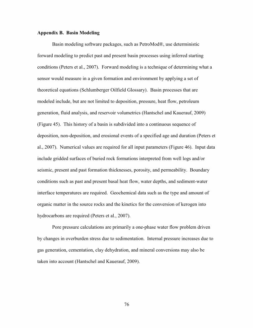
76
Appendix B. Basin Modeling
Basin modeling software packages, such as PetroMod®, use deterministic
forward modeling to predict past and present basin processes using inferred starting
conditions (Peters et al., 2007). Forward modeling is a technique of determining what a
sensor would measure in a given formation and environment by applying a set of
theoretical equations (Schlumberger Oilfield Glossary). Basin processes that are
modeled include, but are not limited to deposition, pressure, heat flow, petroleum
generation, fluid analysis, and reservoir volumetrics (Hantschel and Kauerauf, 2009)
(Figure 45). This history of a basin is subdivided into a continuous sequence of
deposition, non-deposition, and erosional events of a specified age and duration (Peters et
al., 2007). Numerical values are required for all input parameters (Figure 46). Input data
include gridded surfaces of buried rock formations interpreted from well logs and/or
seismic, present and past formation thicknesses, porosity, and permeability. Boundary
conditions such as past and present basal heat flow, water depths, and sediment-water
interface temperatures are required. Geochemical data such as the type and amount of
organic matter in the source rocks and the kinetics for the conversion of kerogen into
hydrocarbons are required (Peters et al., 2007).
Pore pressure calculations are primarily a one-phase water flow problem driven
by changes in overburden stress due to sedimentation. Internal pressure increases due to
gas generation, cementation, clay dehydration, and mineral conversions may also be
taken into account (Hantschel and Kauerauf, 2009).

Figure B1. Major geological processes in basin modeling (Hantschel and Kauerauf, 2009).
77
. Major geological processes in basin modeling (Hantschel and Kauerauf,
. Major geological processes in basin modeling (Hantschel and Kauerauf,
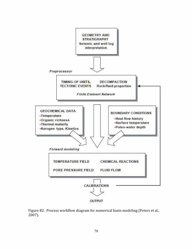
Figure B2. Process workflow diagram for2007).
78
. Process workflow diagram for numerical basin modeling (Peters et al.,
numerical basin modeling (Peters et al.,

79
Temperature calculations are the main goal of heat flow analysis. Past and
present temperatures are necessary for the determination of geochemical reaction rates
such as the conversion of kerogen into petroleum. It is possible to use basin models to
predict vitrinite reflectance. Because vitrinite reflectance is temperature sensitive, it can
be compared to measured data so that uncertain thermal input data, such as paleo heat
flow can be calibrated (Hantschel and Kauerauf, 2009).
Petroleum generation modeling includes the conversion of hydrocarbons from
kerogen (primary cracking) and the secondary cracking of petroleum described with sets
of parallel reactions of decomposition kinetics. Adsorption models are used to describe
the release of hydrocarbons into pore space of the source rock (Hantschel and Kauerauf,
2009).
Darcy flow is used for fluid migration. Darcy flow describes multicomponent
three-phase flow on the basis of pressure gradient and relative permeability. Migration
velocities and accumulation saturations are calculated in one step. Special algorithms are
used to describe migration due to natural fracture propagation and migration across
faults. Diffusion effects may evaluate the transport of light hydrocarbons in the water
phase (Hantschel and Kauerauf, 2009).
Alternatively, migration and accumulation can be modeled using invasion
percolation assuming that on geologic timescales, hydrocarbons move instantaneously
through the basin driven by buoyancy and capillary pressure. Time control is neglected
and the petroleum volume is subdivided into very small amounts. This method is
convenient for one phase flow and in-fault flow (Hantschel and Kauerauf, 2009).
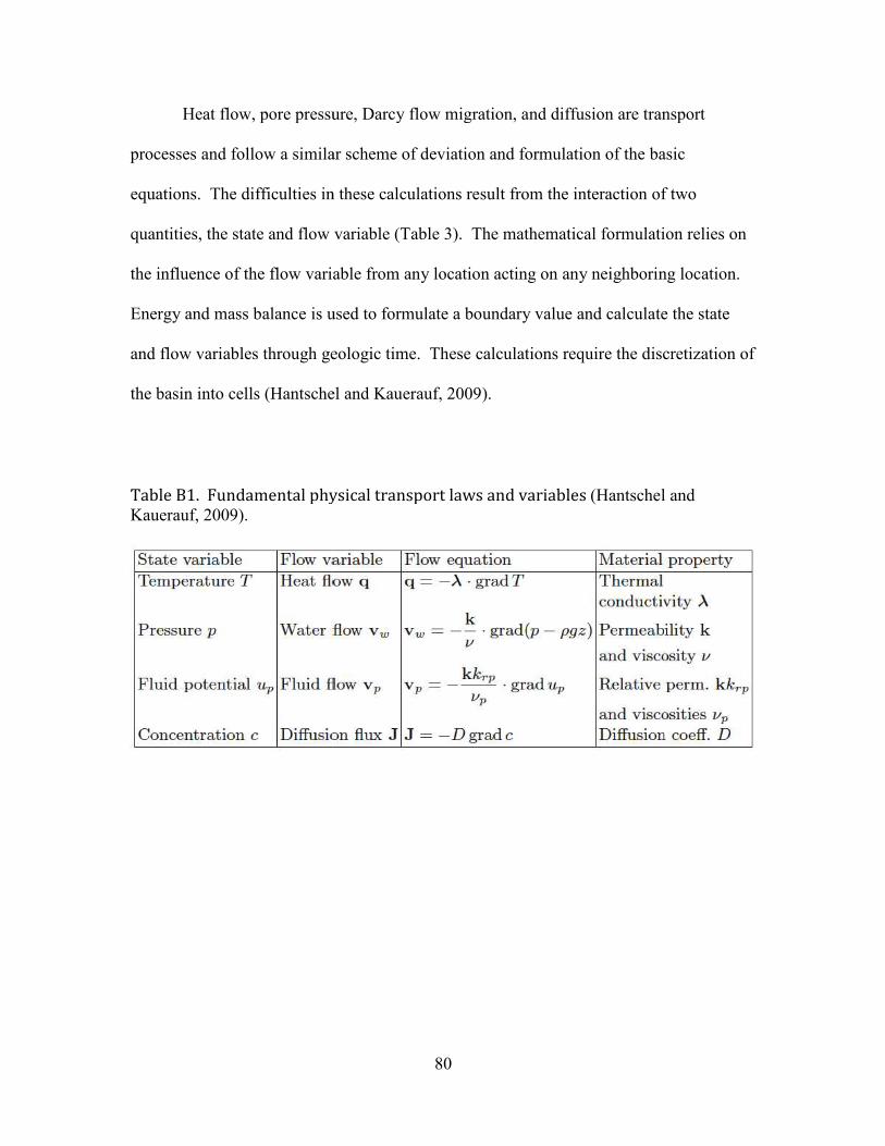
Heat flow, pore pressure,
processes and follow a similar scheme of deviation and formulation of the basic
equations. The difficulties in these calculations result from the interaction of two
quantities, the state and flow variable
the influence of the flow variable from any location acting on any neighboring location.
Energy and mass balance is used to formulate a boundary value and calculate the state
and flow variables through ge
the basin into cells (Hantschel and Kauerauf, 2009)
Table B1. Fundamental physical transport laws and variables Kauerauf, 2009).
80
Heat flow, pore pressure, Darcy flow migration, and diffusion are transport
processes and follow a similar scheme of deviation and formulation of the basic
equations. The difficulties in these calculations result from the interaction of two
state and flow variable (Table 3). The mathematical formulation relies on
the influence of the flow variable from any location acting on any neighboring location.
Energy and mass balance is used to formulate a boundary value and calculate the state
and flow variables through geologic time. These calculations require the discretization of
(Hantschel and Kauerauf, 2009).
. Fundamental physical transport laws and variables (Hantschel and
Darcy flow migration, and diffusion are transport
processes and follow a similar scheme of deviation and formulation of the basic
equations. The difficulties in these calculations result from the interaction of two
). The mathematical formulation relies on
the influence of the flow variable from any location acting on any neighboring location.
Energy and mass balance is used to formulate a boundary value and calculate the state
ologic time. These calculations require the discretization of
(Hantschel and

81
Appendix C. Thermal Maturity Well Name %Ro (PetroMod®) 1-Antium Trust 1.57 1-Beene 1.45 1-Blackmon 1.84 1-Bostwick Holt 1.65 1-Burton Carter 1.43 1-Fuller 1.65 1-Gloria's Ranch 16 1.52 1-Hodges 1.43 1-J Davis 1.55 1-Johnson Odd 2.21 1-Kendrick 1.38 1-Longwood 1.52 1-McCrary 1.71 1-Moncala 31 1.57 1-Morgan 2.26 1-Pardee 3.16 1-Price 0.92 1-Primos 1.04 1-Rabb 2.24 1-Roye 1.82 1-Russ Reality 2.15 1-Sartor 1.89 1-Sec 13 1.49 1-West 28 1.83 1-Foster 1.56 1-Andrews B 1.86 1-Baker 1.62 1-Cates 2.16 1-Crown Zellerbach A 2.34 1-Gish D 1.61 1-Nabors 10 2.03 1-Sibley 2.21 2-Cummings 2.17 25-Benton 1.11 2-Wood 1 2.35 3-Davis 2.18 C1-Tremont Lbr 2.75 Georgia Pacific W 0.91 1-Kennebrew 1.56

82
Vita
Will Torsch was born in Louisville, Kentucky in 1987. He and his family settled
in Birmingham, Alabama, where he grew up. Will earned a Bachelor of Science degree in
geology from Baylor University in May of 2010. He then went on to pursue a Master of
Science degree in the Department of Geology and Geophysics from Louisiana State
University under the advisement of Dr. Jeffrey Nunn. After completing his degree Will
will work full-time as a geophysicist for Newfield Exploration in Houston, Texas.