theory of dielectric

Pu b lish ed by A MS S Press, Wu h an , Ch in aActa Mechanica Solida Sinica, Vol. 23, No. 6, December, 2010 ISSN 0894-9166

THEORY OF DIELECTRIC ELASTOMERS⋆⋆

Z hig ang Suo

⋆

(School of Engineering and Applied Sciences, Kavli Institute for Nanobio Science and Technology, Harvard

University, Cambridge, MA 02138, USA)

Received 25 October 2010, revision received 30 November 2010

ABSTRACT In response to a stimulus, a soft material deforms, and the deformation providesa function. We call such a material a soft active material (SAM). This review focuses on oneclass of soft active materials: dielectric elastomers. When a membrane of a dielectric elastomeris subject to a voltage through its thickness, the membrane reduces thickness and expands area,possibly straining over 100%. The dielectric elastomers are being developed as transducers forbroad applications, including soft robots, adaptive optics, Braille displays, and electric generators.This paper reviews the theory of dielectric elastomers, developed within continuum mechanicsand thermodynamics, and motivated by molecular pictures and empirical observations. The the-ory couples large deformation and electric potential, and describes nonlinear and nonequilibriumbehavior, such as electromechanical instability and viscoelasticity. The theory enables the finiteelement method to simulate transducers of realistic configurations, predicts the efficiency of elec-tromechanical energy conversion, and suggests alternative routes to achieve giant voltage-induceddeformation. It is hoped that the theory will aid in the creation of materials and devices.

KEY WORDS soft active material, dielectric elastomer, electromechanical instability, large de-formation, transducer

I. INTRODUCTION1.1. Soft Active Materials for Soft Machines

The convergence of parts of biology and engineering has created exciting opportunities of discovery,invention and commercialization. The overarching themes include using engineering methods to advancebiology, combining biology and engineering to invent medical procedures, and mimicking biology tocreate engineering devices.

Machines in engineering use mostly hard materials, while machines in nature are often soft. Whatdoes softness impart to the life of animals and plants? A conspicuous feature of life is to receive andprocess information from the environment, and then move. The movements are responsible for diversefunctions, far beyond the function of going from place to place. For example, an octopus can changeits color at an astonishing speed, for camouflage and signaling. This rapid change in color is mediated

⋆ Corresponding author. E-mail: [email protected]⋆⋆ This review draws upon work carried out over the last six years, as a part of a research program on Soft Active Materials,supported at various times by NSF (CMMI-0800161, Large Deformation and Instability in Soft Active Materials), byMURI (W911NF-04-1-0170, Design and Processing of Electret Structures; W911NF-09-1-0476, Innovative Design andProcessing for Multi-Functional Adaptive Structural Materials), and by DARPA (W911NF-08-1-0143, ProgrammableMatter; W911NF-10-1-0113, Cephalopod-Inspired Adaptive Photonic Systems). This work was done in collaborationwith many individuals, as indicated by co-authored papers listed in the references. This review has been revised fromearly drafts using comments received from Siegfried Bauer, Luis Dorfmann, Christoph Keplinger, Guggi Kofod, AdrianKoh, Gabor Kovacs, Liwu Liu, Edoardo Mazza, Arne Schmidt, Carmine Trimarco, and Jian Zhu.

· 550 · ACTA MECHANICA SOLIDA SINICA 2010

Fig. 1. The environment affects a material through diverse stimuli, such as a force, an electric field, a change in pH, anda change in temperature. In response to a stimulus, a soft active material (SAM) deforms. The deformation provides afunction, such as a change in color and a change in flow rate.

by thousands of pigment-containing sacs. Attached to the periphery of each sac are dozens of radialmuscles. By contracting or relaxing the muscles, the sac increases or decreases in area in less than asecond. An expanded sac may be up to about 1 mm in diameter, showing the color. A retracted sacmay be down to about 0.1 mm in diameter, barely visible to the naked eye[1].

As another example, in response to a change in the concentration of salt, a plant can change therate of water flowing through the xylem. This regulation of flow is thought to be mediated by pectins,polysaccharides that are used to make jellies and jams. Pectins are long polymers, crosslinked intoa network. The network can imbibe a large amount of water and swell many times its own volume,resulting in a hydrogel. The amount of swelling changes in response to a change in the concentrationof salt. The change in the volume of the hydrogel alters the size of the microchannels in the xylem,regulating the rate of flow[2].

The above examples concerning animals and plants are intriguing. But many more examples areeverywhere around and inside us. Consider the accommodation of the eye, the beating of the heart, thesound shaped by the vocal folds, and the sound in the ear. Abstracting these biological soft machines, wemay say that a stimulus causes a material to deform, and the deformation provides a function (Fig.1).Connecting the stimulus and the function is the material capable of large deformation in response toa stimulus. We call such a material a soft active material (SAM).

An exciting field of engineering is emerging that uses soft active materials to create soft machines.Soft active materials in engineering are indeed apt in mimicking the salient feature of life: movementsin response to stimuli. An electric field can cause an elastomer to stretch several times its length. Achange in pH can cause a hydrogel to swell many times its volume. These soft active materials arebeing developed for diverse applications, including soft robots, adaptive optics, self-regulating fluidics,programmable haptic surfaces, electric generators, and oilfield management[3–8].

Research in soft active materials has once again brought mechanics to the forefront of humancreativity. The familiar language finds new expressions, and deep thoughts are stimulated by newexperience. To participate in advancing the field of soft active materials and soft machines effectively,mechanicians must retool our laboratories and our software, as well as adapt our theories.

The biological phenomena, as well as the tantalizing engineering applications, have motivated thedevelopment of theories of diverse soft active materials, including dielectric elastomers[9–13], elastomericgels[14–19], polyelectrolytes[20,21], pH-sensitive hydrogels[22–24], and temperature-sensitive hydrogels[25].The theories attempt to answer commonly asked questions. How do mechanics, chemistry, and elec-trostatics work together to generate large deformation? What characteristics of the materials optimizetheir functions? How do molecular processes affect macroscopic behavior? How efficiently can a materialconvert energy from one form to another? The theories are being implemented in software, so that theycan become broadly useful in the creation of materials and devices.

1.2. Dielectric Elastomers

This review will focus on a class of soft active materials: dielectric elastomers. All materials containelectrons and ions—charged particles that move in response to an applied voltage. In a conductor,electrons or ions can move over macroscopic distances. By contrast, in a dielectric, the charged particlesmove relative to one another by small distances. In the dielectric, the two processes—deformation andpolarization—are inherently coupled. All dielectrics are electroactive.

Figure 2 illustrates the principle of operation of a dielectric elastomer transducer. A membrane ofa dielectric elastomer is sandwiched between two electrodes. For the dielectric elastomer to deform

Vol. 23, No. 6 Zhigang Suo: Theory of Dielectric Elastomers · 551 ·

Fig. 2. A dielectric elastomer in the reference state and in a current state.

substantially, the electrodes are made of an even softer substance, with mechanical stiffness lower thanthat of the dielectric elastomer. A commonly used substance for electrodes is carbon grease. When thetransducer is subject to a voltage, charge flows through an external conducting wire from one electrodeto the other. The charges of the opposite signs on the two electrodes cause the membrane to deform.

It was discovered a decade ago that an applied voltage may cause dielectric elastomers to strainover 100%[3]. Because of this large strain, dielectric elastomers are often called artificial muscles. Inaddition to large voltage-induced strains, other desirable attributes of dielectric elastomers includefast response, no noise, light weight, and low cost. The discovery has inspired intense developmentof dielectric elastomers as transducers for diverse applications[26–28]. The discovery has also inspiredrenewed interest in the theory of coupled large deformation and electric field[9–13].

This paper reviews the theory of dielectric elastomers. §II describes the thermodynamics of a trans-ducer of two independent variations. Emphasis is placed on basic ideas: states of the transducer, cyclicoperation of the transducer, region of allowable states, equations of state, stability of a state, andnonconvex free-energy function. These ideas are described in both analytical and geometrical terms.§III develops the theory of homogeneous fields. After setting up a thermodynamic framework for elec-tromechanical coupling, we consider several specific material models: a vacuum as an elastic dielectricof vanishing stiffness, incompressible materials, ideal dielectric elastomers, electrostrictive materials,and nonlinear dielectrics. §IV applies nonequilibrium thermodynamics to dissipative processes, suchas viscoelasticity, dielectric relaxation, and electrical conduction. §V discusses electromechanical in-stability, both as a mode of failure and as a means to achieve giant voltage-induced deformation. §VIoutlines the theory of inhomogeneous fields. The condition for thermodynamic equilibrium is formulatedin terms of a variational statement, as well as in terms of partial differential equations. The model ofideal dielectric elastomers is described. Also described is a finite element method for analyzing elasticdielectric membranes of arbitrary shapes. We perturb a state of static equilibrium to analyze oscillationand bifurcation. We examine the conditions of equilibrium for coexistent phases.

II. THERMODYANMICS OF A TRANSDUCERIt is well appreciated that most fundamental concepts of thermodynamics can be illustrated by

using a fluid—a system capable of two independent variations (thermal and mechanical). The fluidcan serve as the working substance of many devices for thermomechanical energy conversion, includingengines and refrigerators. By analogy, the same concepts of thermodynamics are summarized here forelectromechanical transducers. We are mostly concerned with transducers made of elastomers, which arehighly entropic. To describe such a transducer with two independent variations (electrical and mechan-ical), here we limit ourselves to isothermal processes, removing temperature from explicit consideration.

2.1. States of a Transducer

Figure 3 illustrates a transducer, consisting of a dielectric that separates two electrodes. The trans-ducer is subject to a force P , represented by a weight. The two electrodes are connected through aconducting wire to a voltage Φ, represented by a battery. The weight moves by distance l, and thebattery pumps charge Q to flow through the conducting wire from one electrode to the other.

Because the force P and the voltage Φ can be applied independently, the transducer is capable of twoindependent variations. Consequently, the states of the transducer can be represented graphically on aplane. The two coordinates of the plane may be chosen from variables such as P , Φ, l and Q. Figure 4, for


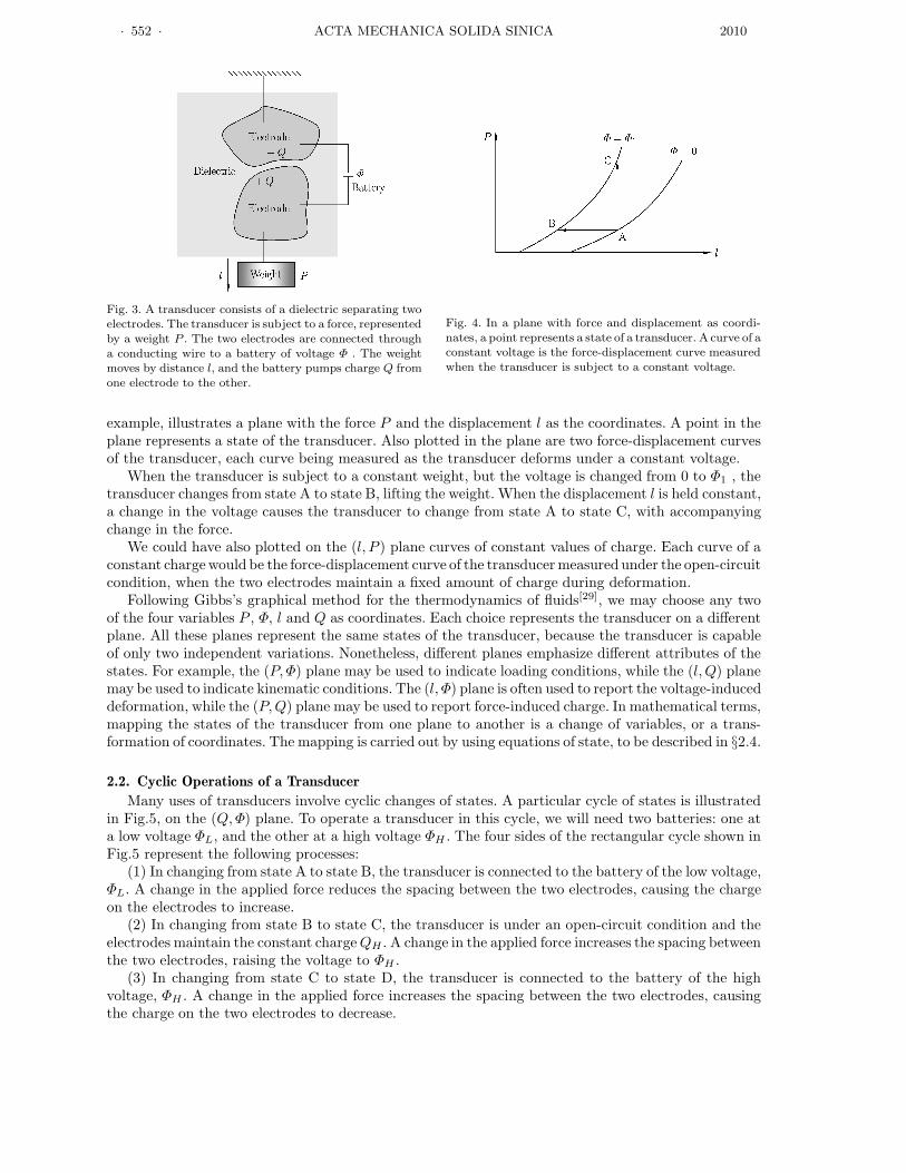
Fig. 3. A transducer consists of a dielectric separating twoelectrodes. The transducer is subject to a force, representedby a weight P . The two electrodes are connected througha conducting wire to a battery of voltage Φ . The weightmoves by distance l, and the battery pumps charge Q fromone electrode to the other.

Fig. 4. In a plane with force and displacement as coordi-nates, a point represents a state of a transducer. A curve of aconstant voltage is the force-displacement curve measuredwhen the transducer is subject to a constant voltage.

example, illustrates a plane with the force P and the displacement l as the coordinates. A point in theplane represents a state of the transducer. Also plotted in the plane are two force-displacement curvesof the transducer, each curve being measured as the transducer deforms under a constant voltage.

When the transducer is subject to a constant weight, but the voltage is changed from 0 to Φ1 , thetransducer changes from state A to state B, lifting the weight. When the displacement l is held constant,a change in the voltage causes the transducer to change from state A to state C, with accompanyingchange in the force.

We could have also plotted on the (l, P ) plane curves of constant values of charge. Each curve of aconstant charge would be the force-displacement curve of the transducer measured under the open-circuitcondition, when the two electrodes maintain a fixed amount of charge during deformation.

Following Gibbs’s graphical method for the thermodynamics of fluids[29], we may choose any twoof the four variables P , Φ, l and Q as coordinates. Each choice represents the transducer on a differentplane. All these planes represent the same states of the transducer, because the transducer is capableof only two independent variations. Nonetheless, different planes emphasize different attributes of thestates. For example, the (P, Φ) plane may be used to indicate loading conditions, while the (l, Q) planemay be used to indicate kinematic conditions. The (l, Φ) plane is often used to report the voltage-induceddeformation, while the (P, Q) plane may be used to report force-induced charge. In mathematical terms,mapping the states of the transducer from one plane to another is a change of variables, or a trans-formation of coordinates. The mapping is carried out by using equations of state, to be described in §2.4.

2.2. Cyclic Operations of a Transducer

Many uses of transducers involve cyclic changes of states. A particular cycle of states is illustratedin Fig.5, on the (Q, Φ) plane. To operate a transducer in this cycle, we will need two batteries: one ata low voltage ΦL, and the other at a high voltage ΦH . The four sides of the rectangular cycle shown inFig.5 represent the following processes:

(1) In changing from state A to state B, the transducer is connected to the battery of the low voltage,ΦL. A change in the applied force reduces the spacing between the two electrodes, causing the chargeon the electrodes to increase.

(2) In changing from state B to state C, the transducer is under an open-circuit condition and theelectrodes maintain the constant charge QH . A change in the applied force increases the spacing betweenthe two electrodes, raising the voltage to ΦH .

(3) In changing from state C to state D, the transducer is connected to the battery of the highvoltage, ΦH . A change in the applied force increases the spacing between the two electrodes, causingthe charge on the two electrodes to decrease.


(4) In changing from state D to state A, the transducer is under an open-circuit condition andthe electrodes maintain the constant charge QL. A change in the applied force decreases the spacingbetween the two electrodes, lowering the voltage to ΦL.

This cycle of operation of an electromechanical transducer is analogous to the Carnot cycle, providedwe replace voltage with temperature, and replace charge with entropy. During the cycle, the transducerreceives mechanical work from the environment, draws an amount of charge from the low-voltage battery,and deposits the same amount of charge to the high-voltage battery. Thus, the transducer is a generator,producing electric energy by receiving mechanical work. The mechanical work can be done, for example,by an animal or human during walking. The mechanical work can also be done on a large scale, forexample, by ocean waves.

Indeed, a closed curve of any shape on the (Q, Φ)plane represents a cyclic operation of the trans-ducer. To operate such a cycle would require avariable-voltage source. The amount of energy con-verted per cycle is given by the area enclosed by thecycle on the (Q, Φ) plane. When the states cyclecounterclockwise on the (Q, Φ) plane, the trans-ducer is a generator, converting mechanical energyto electrical energy. When the states cycle clock-wise on the (Q, Φ) plane, the transducer is an ac-tuator, converting electrical energy to mechanicalenergy.

Cyclic operation of a transducer can also berepresented on the (l, P ) plane. Figure 4 already

Fig. 5 In a plane with voltage and charge as coordinates, apoint represents a state of a transducer. A use of the trans-ducer typically involves a cyclic change of the state. The rect-angle represents a cycle involving two levels of voltage and twovalues of charge.

contains force-displacement curves measured with two values of constant voltage. We could add force-displacement curves measured with two values of constant charge. The four curves would represent thesame cycle of operation as that shown in Fig.5.

2.3. Modes of Failure and Region of Allowable States

A transducer may fail in multiple modes, such as mechanical rupture, electrical breakdown, elec-tromechanical instability, and loss of tension[30–32]. The critical condition for each mode of failure canbe represented on the (Q, Φ) plane by a curve. Curves of all modes of failure bound in the plane aregion, which we call the region of allowable states of the transducer. Such graphic methods have beenused to optimize actuators[33,34] and calculate the maximal energy of conversion for generators[35–37].Figure 6 shows an example[35]. By transformations of coordinates, we can represent the same modes of

Fig. 6. A state of a dielectric membrane is represented by a point in the charge-voltage plane[35]. The coordinates are givenin dimensionless forms, with the horizontal axis being the normalized charge, and the vertical axis being the normalizedvoltage. Plotted are curves representing various modes of failure: electrical breakdown (EB), electromechanical instability(EMI ), loss of tension (s = 0), and rupture by stretch (λ = λR). These curves bound the region of allowable states of thetransducer. A cycle involving two levels of voltage and two values of charge is represented by dotted lines.


failure on planes (l, P ), (l, Q), etc.

2.4. Equations of State

We will analyze isothermal processes of a transducer, and remove temperature from explicit consid-eration. A main component of the transducer is an elastomer—a three-dimensional network of long andflexible polymer chains. The thermodynamic behavior of the transducer is highly entropic, characterizedby the Helmholtz free energy, which we denote as F .

On dropping a small distance δl, the weight does work Pδl. On pumping a small amount of chargeδQ, the battery does work ΦδQ. The force is work-conjugate to the displacement, and the voltage iswork-conjugate to the charge. When the transducer equilibrates with the applied force and the appliedvoltage, the change in the free energy of the transducer equals the sum of the work done by the weightand the work done by the battery:

δF = Pδl + ΦδQ (1)

This condition of equilibrium holds for arbitrary and independent small variations δl and δQ.The two independent variables (l, Q) characterize the state of the transducer. The Helmholtz free

energy of the transducer is a function of the two independent variables:

F = F (l, Q) (2)

Associated with small variations δl and δQ, the free energy varies by

δF =∂F (l, Q)

∂lδl +

∂F (l, Q)

∂QδQ (3)

A comparison of Eqs.(1) and (3) gives[

∂F (l, Q)

∂l− P

]

δl +

[

∂F (l, Q)

∂Q− Φ

]

δQ = 0 (4)

When the transducer equilibrates with the weight and the battery, the condition of equilibrium (4)holds for independent and arbitrary variations δl and δQ. Consequently, in equilibrium, the coefficientsof the two variations in Eq.(4) both vanish, giving

P =∂F (l, Q)

∂l(5)

Φ =∂F (l, Q)

∂Q(6)

Once the free-energy function F (l, Q) is known, Eqs.(5) and (6) express P and Φ as functions of l andQ. That is, the two equations give the force and voltage needed to cause a certain displacement and acertain charge. The two equations (5) and (6) constitute the equations of state of the transducer. Theequations represent the transformations that map the states of the transducer from one thermodynamicplane to another.

Equation (5) can be used to determine the free-energy function from the force-displacement curvesof the transducer measured under the open-circuit conditions, when the electrodes maintain constantcharges. For each value of Q, the free energy is the area under the force-displacement curve. Sim-ilarly, Eq.(6) can be used to determine the free-energy function from the voltage-charge curves ofthe transducer. As mentioned before, (l, P ) and(Q, Φ) are convenient planes to represent the statesof the transducer when we wish to highlight workand energy.

As an illustration, consider a parallel-platecapacitor—two plates of electrodes separated bya thin layer of a vacuum (Fig.7). The separation lbetween the two electrodes may vary, but the areaA of either electrode remains fixed. Recall the ele-mentary fact that the amount of charge on either

Fig. 7 A parallel-plate capacitor consists of two electrodesseparated by a thin gap of a vacuum. When a voltage is ap-plied, the two electrodes attract each other. The electrostaticattraction is balanced by applying a force.


electrode is linear in the voltage:

Φ =lQ

ε0A(7)

where ε0 is the permittivity of the vacuum. Inserting Eq.(7) into Eq.(6), and integrating Eq.(6) withrespect to Q while holding l fixed, we obtain that

F (l, Q) =lQ2

2ε0A(8)

Inserting Eq.(8) into Eq.(5), we obtain that

P =Q2

2Aε0(9)

Equations (7) and (9) constitute the equations of state of the parallel-plate capacitor. They arereadily interpreted. The applied voltage causes charge to flow from one electrode to the other, so thatone electrode is positively charged, and the other negatively charged. Equation (7) relates the chargeto the applied voltage. The oppositely charged electrodes attract each other. To maintain equilibrium,a force need be applied to each electrode. Equation (9) relates the applied force to the charge.

Define the electric field by E = Φ/l and the stress by σ = P/A. Rewrite Eq.(9) as

σ =1

2ε0E

2 (10)

This equation gives the stress needed to be applied to the electrodes to counteract the electrostaticattraction. This stress is known as the Maxwell stress.

2.5. Stability of a State against Linear Perturbation

For a given transducer, the free energy F (l, Q) may take a complicated functional form. The equationsof state, Eqs.(5) and (6), are in general nonlinear. If the transducer operates in the neighborhood ofa particular state (l, Q), the equations of state can be linearized in this neighborhood, written in anincremental form:

δP =∂2F (l, Q)

∂l2δl +

∂2F (l, Q)

∂Q∂lδQ (11)

δΦ =∂2F (l, Q)

∂l∂Qδl +

∂2F (l, Q)

∂Q2δQ (12)

The increments of the loads, δP and δΦ, are linear in the increments of the kinematic variables,δl and δQ. This procedure is known as linear perturbation. We call ∂2F (l, Q) /∂l2 the mechanicaltangent stiffness of the transducer, and ∂2F (l, Q) /∂Q2 the electrical tangent stiffness of the trans-ducer. The two electromechanical coupling effects are both characterized by the same cross derivative,∂2F (l, Q) /(∂l∂Q) = ∂2F (l, Q) /(∂Q∂l). The matrix

H (l, Q) =

∂2F (l, Q)

∂l2∂2F (l, Q)

∂Q∂l∂2F (l, Q)

∂l∂Q

∂2F (l, Q)

∂Q2

(13)

is known as the Hessian of the free-energy function F (l, Q).As mentioned above, a state of the transducer can be represented by a point in the (l, Q) plane,

as well as by a point in the (P, Φ) plane. For the same state of the transducer, the point in the (l, Q)plane is mapped to the point in the (P, Φ) plane by the equations of state, (5) and (6). The mappingmay not always be invertible. That is, given a pair of the loads (P, Φ), the equations of state may notbe invertible to determine a state (l, Q). For example, Eqs.(11) and (12) are not invertible when theHessian is a singular matrix, detH = 0.

This singularity may be understood in terms of thermodynamics. The transducer and the loadingmechanisms (i.e., the weight and the battery) together constitute a thermodynamic system. The free


energy of the system is the sum of the free energies of the individual parts—the transducer, the weight,and the battery. The free energy (i.e., the potential energy) of a constant weight is −Pl. The free energyof a battery of a constant voltage is −ΦQ . Consequently, the free energy of the thermodynamic systemcombining the transducer and the loading mechanisms is

G (l, Q) = F (l, Q) − Pl − ΦQ (14)

The system has two independent variables, l and Q.Thermodynamics requires that the system should reach a stable state of equilibrium when the free-

energy function G (l, Q) is a minimum against small changes in l and Q. When the weight moves by δland the battery pumps charges δQ, the free energy of the system varies by

δG =

[

∂F (l, Q)

∂l− P

]

δl +

[

∂F (l, Q)

∂Q− Φ

]

δQ +∂2F (l, Q)

2∂l2(δl)

2

+∂2F (l, Q)

∂l∂Q(δl) (δQ) +

∂2F (l, Q)

2∂Q2(δQ)2 (15)

We have expanded the Taylor series of the function F (l, Q) up to terms quadratic in δl and δQ. In astate of equilibrium, the coefficients of the first-order variations vanish, recovering the equations of state(5) and (6). To ensure that this state of equilibrium minimizes G, the sum of the second-order variationsmust be positive for arbitrary combination of δl and δQ. That is, a state of equilibrium is stable againstsmall perturbation if the Hessian of the free energy of the transducer, H (l, Q), is positive-definite. Thetwo-by-two matrix is positive-definite if and only if

∂2F (l, Q)

∂l2> 0,

∂2F (l, Q)

∂Q2> 0,

[

∂2F (l, Q)

∂l2

] [

∂2F (l, Q)

∂Q2

]

>

[

∂2F (l, Q)

∂l∂Q

]2

(16)

When the Hessian of the free energy function is positive-definite, the function F (l, Q) is convex at thisstate (l, Q).

As an illustration, consider the parallel-plate capacitor again. Given the free-energy function (8),the second derivatives are

∂2F (l, Q)

∂l2= 0,

∂2F (l, Q)

∂Q2=

l

ε0A,

[

∂2F (l, Q)

∂l∂Q

]

=Q

ε0A(17)

Consequently, the Hessian is not positive-definite in any state of equilibrium. That is, the parallel-platecapacitor subject to a constant force and a constant voltage cannot reach a stable state of equilibrium.The conclusion is readily understood. The weight is independent of the separation between the plates,but the electrostatic attractive force increases as the separation decreases. Subject to a fixed weight,the two plates will be pulled apart if the voltage is low, and will be pulled together if the voltage ishigh.

The capacitor can be stabilized by a modification of the loading mechanisms. For example, we canreplace the weight with a spring that restrains the relative movement of the plates. Let K be the stiffnessof the spring, and l0be the separation between the electrodes when the spring is unstretched, so thatthe force in the spring is P = K (l0 − l). The free energy of the system is the sum of the free energiesof the capacitor, the spring and the battery:

G (l, Q) =lQ2

2ε0A+

1

2K (l − l0)

2− ΦQ (18)

In a state of equilibrium, the first derivatives of G (l, Q) vanish, giving the same equations of state asEqs.(10) and (12). The state of equilibrium is stable if and only if the Hessian of G (l, Q) is positive-definite. The second derivatives of the function G (l, Q) are

∂2G (l, Q)

∂l2= K,

∂2G (l, Q)

∂Q2=

l

ε0A,

∂2G (l, Q)

∂l∂Q=

Q

ε0A(19)

A state of equilibrium (l, Q) is stable if and only if

Kl

ε0A>

(

Q

ε0A

)2

(20)

Thus, the transducer is stable when the spring is stiff and the applied voltage is small.


2.6. Nonconvex Free-Energy Surface

Following Gibbs[38], we may interpret above analytical statements geometrically. This geometricrepresentation not only shows the geometric nature of the stability against linear perturbation, butalso shows the possibility of coexistent states.

Consider a three-dimensional space with (l, Q) as the horizontal plane, and F as the vertical axis.In this space, the Helmholtz free energy F (l, Q) is represented by a surface. Consider an inclined planepassing through the origin of the space, with P being the slope of the inclined plane with respectto the l axis, and Φ being the slope of the inclined plane with respect to the Q axis. According toEq.(14), the vertical distance between the surface F (l, Q) and the inclined plane is the function G (l, Q).Thermodynamics dictates that this vertical distance G (l, Q) should minimize when the transducerequilibrates with the loads (P, Φ).

Picture a plane simultaneously parallel to the inclined plane and tangent to the surface F (l, Q).From the geometry, the tangent point minimizes the vertical distance G (l, Q) if the surface F (l, Q) isabove the tangent plane—that is, if the surface F (l, Q) is convex at the state (l, Q).

When the loads (P, Φ) change gradually, the inclined plane rotates, and the associated tangent planerolls along the free-energy surface. If the surface F (l, Q) is globally convex, every tangent plane touchesthe surface at only one point, and only one state of equilibrium is associated with a pair of given loads(P, Φ). By contrast, if part of the surface F (l, Q) is concave, a tangent plane may touch the surface attwo points, and the two states of equilibrium are associated with a pair of given loads (P, Φ).

It was discovered that the free-energy functions for dielectric elastomers are typically nonconvex[39].Associated with a given set of loads, two states of equilibrium may coexist. This topic will be discussedin §5.4 and §6.8.

III. HOMOGENEOUS FIELDWe now develop a field theory of deformable dielectrics. The field theory assumes that a body is a

sum of many small pieces, and the field in each small piece is homogeneous. This assumption enablesus to define quantities per unit length, per unit area, and per unit volume. This section focuses on thehomogeneous field of a small piece, and §VI considers inhomogeneous field in the body by summing upsmall pieces.

This section begins by setting up a thermodynamic framework for electromechanical coupling. Wethen consider several specific material models: a vacuum as an elastic dielectric of vanishing rigidity,incompressible materials, ideal dielectric elastomers, electrostrictive materials, and nonlinear dielectrics.

3.1. Condition of Thermodynamic Equilibrium

With reference to Fig.2, consider a membrane of an elastic dielectric, sandwiched between twocompliant electrodes. In the reference state, the dielectric is subject to neither force nor voltage, andthe dielectric is of dimensions L1, L2 and L3. In the current state, the dielectric is subject to forces P1,P2 and P3, and the two electrodes are connected to a battery of voltage Φ through a conducting wire.In the current state, the dimensions of the dielectric become l1, l2 and l3, the two electrodes accumulateelectric charges ±Q, and the Helmholtz free energy of the membrane is F .

When the dimensions of the dielectric change by δl1, δl2 and δl3, the forces do work P1δl1 +P2δl2 +P3δl3. When a small quantity of charge δQ flows through the conducting wire, the voltage does workΦδQ. When the dielectric equilibrates with the forces and the voltage, the increase in the free energyequals the work done:

δF = P1δl1 + P2δl2 + P3δl3 + ΦδQ (21)

The condition of equilibrium (21) holds for arbitrary small variations of the four independent variables,l1, l2, l3 and Q.

3.2. Equations of State in Terms of Nominal Quantities

Define the nominal density of the Helmholtz free energy by W = F/(L1L2L3), stretches by λ1 =l1/L1, λ2 = l2/L2 and λ3 = l3/L3, nominal stresses by s1 = P1/ (L2L3) , s2 = P2/ (L1L3) and s3 =P3/ (L1L2), nominal electric field by E = Φ/L3, and nominal electric displacement by D = Q/(L1L2).


The amount of charge on either electrode relates to the nominal electric displacement by Q = DL1L2.When the membrane is subject to forces and voltage, the variation of the charge is δQ = L1L2δD.

Divide both sides of Eq.(21) by L1L2L3, the volume of the membrane in the reference state. Weobtain that

δW = s1δλ1 + s2δλ2 + s3δλ3 + EδD (22)

This condition of equilibrium holds for arbitrary and independent small variations δλ1, δλ2, δλ3 andδD.

As a material model, the nominal density of the Helmholtz free energy is prescribed as a functionof the four independent variables:

W = W(

λ1, λ2, λ3, D)

(23)

Inserting Eq.(23) into Eq.(22), we obtain that(

∂W

∂λ1− s1

)

δλ1 +

(

∂W

∂λ2− s2

)

δλ2 +

(

∂W

∂λ3− s3

)

δλ3 +

(

∂W

∂D− E

)

δD = 0 (24)

This condition of equilibrium holds for arbitrary and independent small variations δλ1, δλ2, δλ3 andδD. Consequently, when the dielectric equilibrates with the applied forces and the applied voltage, thecoefficient in front of each variation in Eq.(24) vanishes, giving

s1 =∂W

(

λ1, λ2, λ3, D)

∂λ1(25)

s2 =∂W

(

λ1, λ2, λ3, D)

∂λ2(26)

s3 =∂W

(

λ1, λ2, λ3, D)

∂λ3(27)

E =∂W

(

λ1, λ2, λ3, D)

∂D(28)

The equations of state (25)-(28) give the values of the forces and voltage needed to equilibrate with

the dielectric in the state(

λ1, λ2, λ3, D)

once the free-energy function W(

λ1, λ2, λ3, D)

is prescribed

as a material model.In the above, we have defined stresses as applied forces divided by areas. In the absence of the

applied forces, the stresses in the dielectric vanish. The stresses are zero even when the voltage causesthe dielectric to deform. Thus, when the battery applies a voltage to the dielectric, the positive chargeon one electrode and the negative charge on the other electrode cause the dielectric to thin down.We simply report what we have observed in this experiment: the voltage causes the dielectric to de-form. We do not jump to the conclusion that the voltage causes a compressive stress. In this regard,we view the deformation caused by the voltage in the same way as we view the deformation causedby a change in temperature: both are stress-free deformation, so long as the material is unconstrained[12].

3.3. Equations of State in Terms of True Quantities

In §3.2, we have represented the equations of state in terms of the nominal quantities. We nowrepresent the equations of state in terms of true quantities. The two sets of equations describe the samecondition of thermodynamic equilibrium, but they are convenient under different circumstances.

Define the true stresses by σ1 = P1/ (l2l3), σ2 = P2/ (l1l3) and σ3 = P3/ (l1l2), true electric field byE = Φ/l3, and true electric displacement by D = Q/(l1l2). The amount of charge on either electroderelates to the electric displacement by Q = Dl1l2. When the membrane is subject to forces and voltage,all three quantities D, l1 and l2 can vary, so that the variation of the charge is

δQ = Dl2δl1 + Dl1δl2 + l1l2δD (29)


This equation should be contrasted with δQ = L1L2δD , where the nominal electric displacement isused.

Dividing both sides of Eq.(21) by L1L2L3, the volume of the membrane in the reference state, andusing Eq.(29), we obtain that

δW = (σ1 + DE)λ2λ3δλ1 + (σ2 + DE)λ1λ3δλ2 + σ3λ1λ2δλ3 + λ1λ2λ3EδD (30)

The condition of equilibrium (30) holds for arbitrary and independent variations δλ1, δλ2 , δλ3 andδD.

As a material model, the nominal density of Helmholtz free energy is taken to be a function of thefour independent variables,

W = W (λ1, λ2, λ3, D) (31)

Comparing Eqs.(23) and (31), we remark that here the true electric displacement, rather than thenominal electric displacement, is used as an independent variable.

Inserting Eq.(31) into Eq.(30), we obtain that

[

∂W

∂λ1− (σ1 + DE)λ2λ3

]

δλ1 +

[

∂W

∂λ2− (σ2 + DE)λ1λ3

]

δλ2

+

(

∂W

∂λ3− σ3λ1λ2

)

δλ3 +

(

∂W

∂D− λ1λ2λ3E

)

δD = 0 (32)

This condition of equilibrium holds for arbitrary and independent small variations δλ1, δλ2, δλ3 andδD. Consequently, when the dielectric equilibrates with the applied forces and the applied voltage, thecoefficient in front of each variation in Eq.(32) vanishes, giving

σ1 =∂W (λ1, λ2, λ3, D)

λ2λ3∂λ1− ED (33)

σ2 =∂W (λ1, λ2, λ3, D)

λ1λ3∂λ2− ED (34)

σ3 =∂W (λ1, λ2, λ3, D)

λ1λ2∂λ3(35)

E =∂W (λ1, λ2, λ3, D)

λ1λ2λ3∂D(36)

Equations (33)-(36) constitute the equations of state for an elastic dielectric once the function W (λ1,λ2, λ3, D) is given. These equations suggest that electromechanical coupling be classified into two kinds.First, the geometric coupling is characterized by Eq.(29), which results in the term DE in Eqs.(33) and(34). Second, the material coupling is characterized by the function W (λ1, λ2, λ3, D). Several specificmaterial models are described next.

3.4. Vacuum

We think of a vacuum as an elastic dielectric with vanishing stiffness, undergoing a homogenousdeformation λ1, λ2, and λ3. Recall an elementary fact that in the vacuum the electric field relates tothe electric displacement as E = D/ε0. Integrating Eq.(30) with respect to D, while holding λ1, λ2 andλ3 fixed, we obtain that

W (λ1, λ2, λ3, D) =D2

2ε0λ1λ2λ3 (37)

This expression recovers a familiar result in electrostatics: D2/ (2ε0) is the electrostatic energy per unitvolume in the vacuum. The factor λ1λ2λ3 appears in Eq.(37) because we have defined W as the nominaldensity of energy.


Inserting Eq.(37) into Eqs.(33)-(35), we obtain that

σ1 = −1

2ε0E

2 (38)

σ2 = −1

2ε0E

2 (39)

σ3 =1

2ε0E

2 (40)

Equations (38)-(40) recover the stresses obtained by Maxwell[40]. They are valid in the vacuum whenthe electric field is in direction 3.

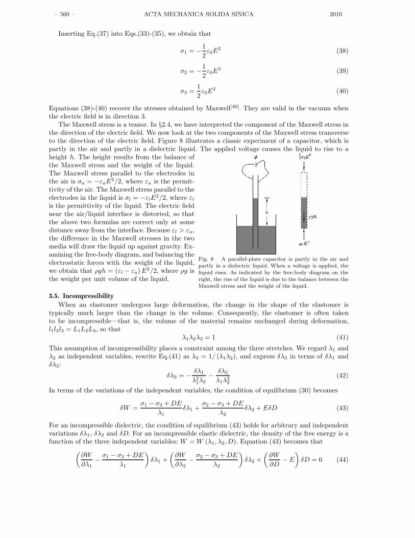
The Maxwell stress is a tensor. In §2.4, we have interpreted the component of the Maxwell stress inthe direction of the electric field. We now look at the two components of the Maxwell stress transverseto the direction of the electric field. Figure 8 illustrates a classic experiment of a capacitor, which ispartly in the air and partly in a dielectric liquid. The applied voltage causes the liquid to rise to aheight h. The height results from the balance ofthe Maxwell stress and the weight of the liquid.The Maxwell stress parallel to the electrodes inthe air is σa = −εaE2/2, where εa is the permit-tivity of the air. The Maxwell stress parallel to theelectrodes in the liquid is σl = −εlE

2/2, where εl

is the permittivity of the liquid. The electric fieldnear the air/liquid interface is distorted, so thatthe above two formulas are correct only at somedistance away from the interface. Because εl > εa,the difference in the Maxwell stresses in the twomedia will draw the liquid up against gravity. Ex-amining the free-body diagram, and balancing theelectrostatic forces with the weight of the liquid,we obtain that ρgh = (εl − εa)E2/2, where ρg isthe weight per unit volume of the liquid.

Fig. 8 A parallel-plate capacitor is partly in the air andpartly in a dielectric liquid. When a voltage is applied, theliquid rises. As indicated by the free-body diagram on theright, the rise of the liquid is due to the balance between theMaxwell stress and the weight of the liquid.

3.5. Incompressibility

When an elastomer undergoes large deformation, the change in the shape of the elastomer istypically much larger than the change in the volume. Consequently, the elastomer is often takento be incompressible—that is, the volume of the material remains unchanged during deformation,l1l2l3 = L1L2L3, so that

λ1λ2λ3 = 1 (41)

This assumption of incompressibility places a constraint among the three stretches. We regard λ1 andλ2 as independent variables, rewrite Eq.(41) as λ3 = 1/ (λ1λ2), and express δλ3 in terms of δλ1 andδλ2:

δλ3 = −δλ1

λ21λ2

−δλ2

λ1λ22

(42)

In terms of the variations of the independent variables, the condition of equilibrium (30) becomes

δW =σ1 − σ3 + DE

λ1δλ1 +

σ2 − σ3 + DE

λ2δλ2 + EδD (43)

For an incompressible dielectric, the condition of equilibrium (43) holds for arbitrary and independentvariations δλ1, δλ2 and δD. For an incompressible elastic dielectric, the density of the free energy is afunction of the three independent variables: W = W (λ1, λ2, D). Equation (43) becomes that

(

∂W

∂λ1−

σ1 − σ3 + DE

λ1

)

δλ1 +

(

∂W

∂λ2−

σ2 − σ3 + DE

λ2

)

δλ2 +

(

∂W

∂D− E

)

δD = 0 (44)


Because δλ1, δλ2 and δD are independent variations, the condition of equilibrium (44) is equivalent tothree equations:

σ1 − σ3 = λ1∂W (λ1, λ2, D)

∂λ1− ED (45)

σ2 − σ3 = λ2∂W (λ1, λ2, D)

∂λ2− ED (46)

E =∂W (λ1, λ2, D)

∂D(47)

Once the function W (λ1, λ2, D) is given for an incompressible dielectric elastomer, the four equations,(41) and (45)-(47), constitute the equations of state.

3.6. Ideal Dielectric ElastomersAn elastomer is a three-dimensional network

of long and flexible polymers, held together bycrosslinks (Fig.9). Each polymer chain consists ofa large number of monomers. Consequently, thecrosslinks have negligible effect on the polarizationof the monomers—that is, the elastomer can polar-ize nearly as freely as a polymer melt. This molec-ular picture is consistent with the following exper-imental observation: the permittivity changes byonly a few percent when a membrane of an elas-

Fig. 9 An elastomer is a three dimensional network of longand flexible polymer chains. Each polymer chain consists ofa large number of monomers.

tomer is stretched to increase the area 25 times[41].

As an idealization, we may assume that the dielectric behavior of an elastomer is exactly the sameas that of a polymer melt—that is, the true electric field relates to the true electric displacement as

E = D/ε (48)

where ε is the permittivity of the elastomer, taken to be a constant independent of deformation. InsertingEq.(48) into Eq.(43), and integrating Eq.(43) with respect to D while holding λ1 and λ2 fixed, we obtainthat

W (λ1, λ2, D) = Ws (λ1, λ2) +D2

2ε(49)

The constant of integration, Ws (λ1, λ2), is the Helmholtz free energy associated with the stretchingof the elastomer. The material is also taken to be incompressible, λ1λ2λ3 = 1. This material model(49) is known as the model of ideal dielectric elastomers[39]. In this model (49), the stretches and thepolarization contribute to the free energy independently. Consequently, the electromechanical couplingin an ideal dielectric elastomer is purely a geometric effect, in the sense as remarked at the end of §3.3.

Inserting Eq.(49) into Eqs.(45) and (46), and also using Eq.(48), we obtain that

σ1 − σ3 = λ1∂Ws (λ1, λ2)

∂λ1− εE2 (50)

σ2 − σ3 = λ2∂Ws (λ1, λ2)

∂λ2− εE2 (51)

Equations (41), (48), (50) and (51) constitute the equations of state for an incompressible, ideal dielectricelastomer, provided the permittivity ε and the function Ws (λ1, λ2) are given. These equations ofstate have been used almost exclusively in all analyses of dielectric elastomers, and agree well withexperimentally measured equations of state[42]. The equations are usually justified in terms of theMaxwell stress[3], and can be interpreted using the model of ideal dielectric elastomers[39]. That is,the Maxwell stress is valid when the dielectric behavior of the material is liquid-like, unaffected bydeformation.


As shown in Eqs.(50) and (51), a through-thickness voltage induces a compressive stress of magnitudeεE2 in the two in-plane directions. This magnitude is twice the magnitude of the Maxwell stress. Theapparent difference is readily understood (Fig.10). Because the elastomer is taken to be incompressible,superposition of a state of hydrostatic stress does not affect the state of deformation. Start from thestate of triaxial stresses

(

−εE2/2, −εE2/2, +εE2/2)

, as derived by Maxwell. A superposition of a

state of hydrostatic stress(

+εE2/2, +εE2/2, +εE2/2)

gives a state of uniaxial stress(

0, 0, +εE2)

. A

superposition of a state of hydrostatic stress(

−εE2/2, −εE2/2, −εE2/2)

gives a state of biaxial stress(

−εE2, −εE2, 0)

. For an incompressible material, the three states of stress illustrated in Fig.10 causethe same state of deformation.

Fig. 10. A dielectric in three states of stresses.

The free energy due to the stretching of the elastomer, Ws (λ1, λ2), may be selected from a largemenu of well-tested functions in the theory of rubber elasticity. For example, the neo-Hookean modeltakes the form

Ws =µ

2

(

λ21 + λ2

2 + λ23 − 3

)

(52)

where µ is the small-stress shear modulus. This free energy is due to the change of entropy when polymerchains are stretched[43].

In an elastomer, each individual polymer chain has a finite contour length. When the elastomer issubject to no loads, the polymer chains are coiled, allowing a large number of conformations. Subjectto loads, the polymer chains become less coiled. As the loads increase, the end-to-end distance of eachpolymer chain approaches the finite contour length, and the elastomer approaches a limiting stretch. Onapproaching the limiting stretch, the elastomer stiffens steeply. This effect is absent in the neo-Hookeanmodel, but is represented by the Arruda and Boyce model[44] and the Gent model[45]. The latter takesthe form

Ws = −µJlim

2log

(

1 −λ2

1 + λ22 + λ2

3 − 3

Jlim

)

(53)

where µ is the small-stress shear modulus, and Jlim is a constant related to the limiting stretch. Thestretches are restricted as 0 ≤

(

λ21 + λ2

2 + λ23 − 3

)

/Jlim < 1. When(

λ21 + λ2

2 + λ23 − 3

)

/Jlim → 0, theTaylor expansion of Eq.(53) is Eq.(52). That is, the Gent model recovers the neo-Hookean model whendeformation is small compared to the limiting stretch. When

(

λ21 + λ2

2 + λ23 − 3

)

/Jlim → 1, the freeenergy diverges, and the elastomer approaches the limiting stretch.

3.7. Electrostriction

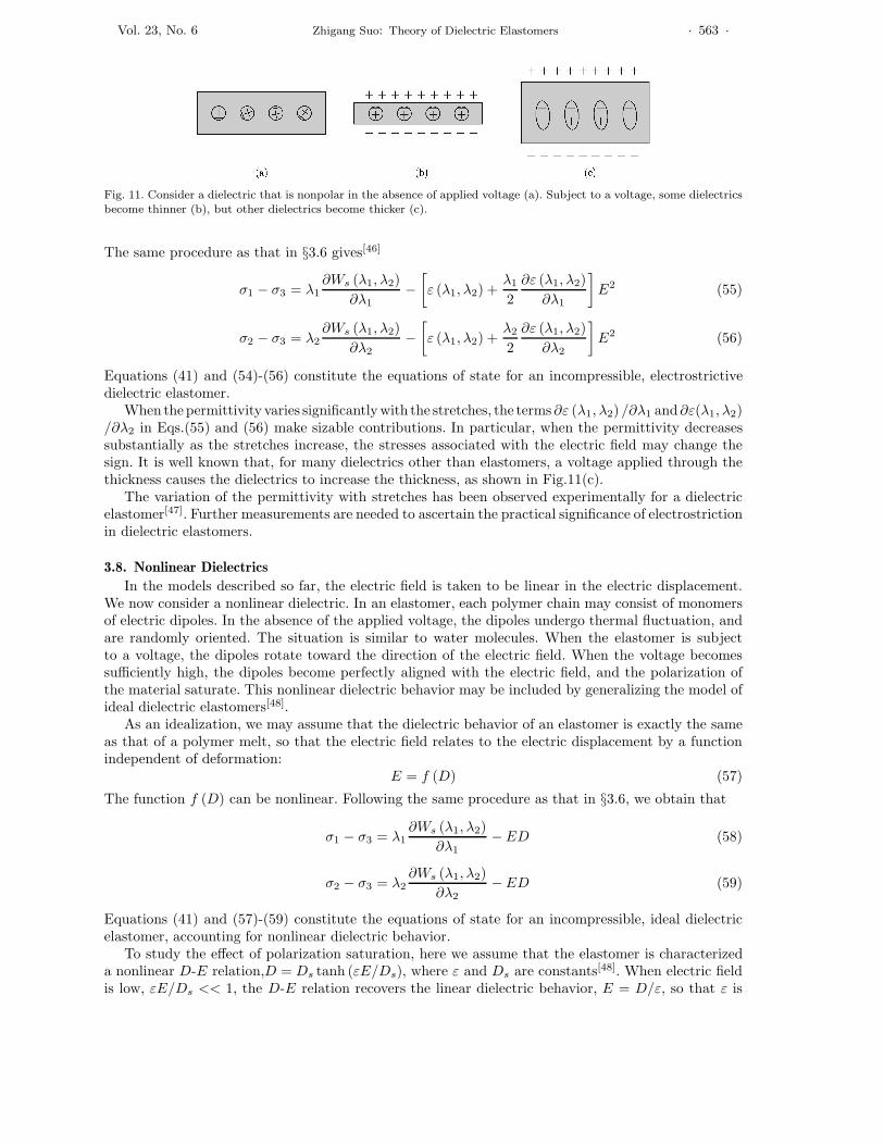
Subject to a voltage through the thickness, some dielectrics become thinner, but other dielectricsbecome thicker (Fig.11). For dielectrics that are nonpolar in the absence of electric field, the voltage-induced deformation has been analyzed by invoking stresses of two origins: electrostriction and theMaxwell stress. The electrostriction results from the effect of deformation on permittivity.

As a simplest model of electrostriction, we still assume that the true electric field is linear in thetrue electric displacement, but now the permittivity is a function of the stretches. Write the relationbetween the electric field and the electric displacement as

E =D

ε (λ1, λ2)(54)


Fig. 11. Consider a dielectric that is nonpolar in the absence of applied voltage (a). Subject to a voltage, some dielectricsbecome thinner (b), but other dielectrics become thicker (c).

The same procedure as that in §3.6 gives[46]

σ1 − σ3 = λ1∂Ws (λ1, λ2)

∂λ1−

[

ε (λ1, λ2) +λ1

2

∂ε (λ1, λ2)

∂λ1

]

E2 (55)

σ2 − σ3 = λ2∂Ws (λ1, λ2)

∂λ2−

[

ε (λ1, λ2) +λ2

2

∂ε (λ1, λ2)

∂λ2

]

E2 (56)

Equations (41) and (54)-(56) constitute the equations of state for an incompressible, electrostrictivedielectric elastomer.

When the permittivity varies significantlywith the stretches, the terms ∂ε (λ1, λ2) /∂λ1 and∂ε(λ1, λ2)/∂λ2 in Eqs.(55) and (56) make sizable contributions. In particular, when the permittivity decreasessubstantially as the stretches increase, the stresses associated with the electric field may change thesign. It is well known that, for many dielectrics other than elastomers, a voltage applied through thethickness causes the dielectrics to increase the thickness, as shown in Fig.11(c).

The variation of the permittivity with stretches has been observed experimentally for a dielectricelastomer[47]. Further measurements are needed to ascertain the practical significance of electrostrictionin dielectric elastomers.

3.8. Nonlinear Dielectrics

In the models described so far, the electric field is taken to be linear in the electric displacement.We now consider a nonlinear dielectric. In an elastomer, each polymer chain may consist of monomersof electric dipoles. In the absence of the applied voltage, the dipoles undergo thermal fluctuation, andare randomly oriented. The situation is similar to water molecules. When the elastomer is subjectto a voltage, the dipoles rotate toward the direction of the electric field. When the voltage becomessufficiently high, the dipoles become perfectly aligned with the electric field, and the polarization ofthe material saturate. This nonlinear dielectric behavior may be included by generalizing the model ofideal dielectric elastomers[48].

As an idealization, we may assume that the dielectric behavior of an elastomer is exactly the sameas that of a polymer melt, so that the electric field relates to the electric displacement by a functionindependent of deformation:

E = f (D) (57)

The function f (D) can be nonlinear. Following the same procedure as that in §3.6, we obtain that

σ1 − σ3 = λ1∂Ws (λ1, λ2)

∂λ1− ED (58)

σ2 − σ3 = λ2∂Ws (λ1, λ2)

∂λ2− ED (59)

Equations (41) and (57)-(59) constitute the equations of state for an incompressible, ideal dielectricelastomer, accounting for nonlinear dielectric behavior.

To study the effect of polarization saturation, here we assume that the elastomer is characterizeda nonlinear D-E relation,D = Ds tanh (εE/Ds), where ε and Ds are constants[48]. When electric fieldis low, εE/Ds << 1, the D-E relation recovers the linear dielectric behavior, E = D/ε, so that ε is


the small-field permittivity. When the electric field is high, εE/Ds >> 1, the D-E relation becomesD = Ds, so that Ds is the saturated electric displacement.

The effect of polarization saturation is appreciated by inspecting the equations of state, (58) and(59). When the dielectric behavior is linear, D = εE, the term DE recovers the Maxwell stress εE2.As polarization saturates, however, the term DE becomes DsE, which increases with the electric fieldlinearly. Consequently, polarization saturation makes the stress associated with voltage rise less steeply.This behavior may markedly affect electromechanical coupling[48].

IV. NONEQUILIBRIUM THERMODYNAMICS OF DIELECTRIC ELASTOMERSAn elastomer responds to forces and voltage by time-dependent, dissipative processes[49–51]. Vis-

coelastic relaxation may result from slippage between long polymers and rotation of joints betweenmonomers. Dielectric relaxation may result from distortion of electron clouds and rotation of polargroups. Conductive relaxation may result from migration of electrons and ions through the elastomer.This section describes an approach to construct models of dissipative dielectric elastomers, guided bynonequilibrium thermodynamics[52].

Thermodynamics requires that the increase in the free energy should not exceed the total work done,namely,

δF ≤ P1δl1 + P2δl2 + P3δl3 + ΦδQ (60)

For the inequality to be meaningful, the small changes are time-directed: δf means the change of thequantity f from one time to a slightly later time.

Divide both sides of Eq.(60) by the volume of the membrane, L1L2L3, and the thermodynamicinequality becomes

δW ≤ s1δλ1 + s2δλ2 + s3δλ3 + EδD (61)

As a model of the dielectric elastomer, the free-energy density is prescribed as a function:

W = W(

λ1, λ2, λ3, D, ξ1, ξ2, ...)

(62)

We characterize the state of a dielectric by λ1, λ2, λ3 and D, along with additional parameters (ξ1, ξ2, ...).Inspecting Eq.(61), we note that λ1, λ2, λ3 and D are the kinematic parameters through which theexternal loads do work. By contrast, the additional parameters (ξ1, ξ2, ...) are not associated with theexternal loads in this way. These additional parameters describe the degrees of freedom associated withdissipative processes, and are known as internal variables.

Inserting Eq.(62) into Eq.(61), we rewrite the thermodynamic inequality as(

∂W

∂λ1− s1

)

δλ1 +

(

∂W

∂λ2− s2

)

δλ2 +

(

∂W

∂λ3− s3

)

δλ3 +

(

∂W

∂D− E

)

δD +∑

i

∂W

∂ξiδξi ≤ 0 (63)

As time goes forward, this thermodynamic inequality holds for any change in the independent variables(

λ1, λ2, λ3, D, ξ1, ξ2, ...)

. We next specify a model consistent with this inequality.

We assume that the system is in mechanical and electrostatic equilibrium, so that in Eq.(63) thefactors in front of δλ1, δλ2 , δλ3 and δD vanish:

s1 =∂W

(

λ1, λ2, λ3, D, ξ1, ξ2, ...)

∂λ1(64)

s2 =∂W

(

λ1, λ2, λ3, D, ξ1, ξ2, ...)

∂λ2(65)

s3 =∂W

(

λ1, λ2, λ3, D, ξ1, ξ2, ...)

∂λ3(66)

E =∂W

(

λ1, λ2, λ3, D, ξ1, ξ2, ...)

∂D(67)


Equations (64)-(67) constitute the thermodynamic equations of state of the dielectric elastomer.Once the elastomer is assumed to be in mechanical and electrostatic equilibrium, the inequality (63)

becomes

∑

i

∂W(

λ1, λ2, λ3, D, ξ1, ξ2, ...)

∂ξiδξi ≤ 0 (68)

This thermodynamic inequality may be satisfied by prescribing a suitable relation between (δξ1, δξ2, ...)and (∂W/∂ξ1, ∂W/∂ξ2, ...). For example, one may adopt a kinetic model of the type

dξi

dt= −

∑

j

Mij

∂W(

λ1, λ2, λ3, D, ξ1, ξ2, ...)

∂ξj(69)

Here Mij is a positive-definite matrix, which may depend on the independent variables (λ1, λ2,

λ3, D, ξ1, ξ2, ...)

.

To represent a dissipative dielectric elastomer using the above approach, we need to specify a

set of internal variables (ξ1, ξ2, ...), and then specify the functions W(

λ1, λ2, λ3, D, ξ1, ξ2, ...)

and

Mij

(

λ1, λ2, λ3, D, ξ1, ξ2, ...)

. There is considerable flexibility in choosing kinetic models to fulfill the

thermodynamic inequality (68). To develop a kinetic model for a given material, one also draws uponmechanistic pictures and experimental data.

Viscoelastic relaxation is commonly pictured with an array of springs and dashpots, known as therheological models; see recent examples[52,53]. Similarly, dielectric relaxation is commonly pictured withmodels consisting of resistors and capacitors. By contrast, electrical conduction involves the transportof charged species over a long distance. Coupled large deformation and transport of charged speciesare significant in polyelectrolytes[21], and will not be discussed here.

V. ELECTROMECHANICAL INSTABILITYWhile all dielectrics deformunder voltage, the amount of deformationdiffersmarkedly amongdifferent

materials. Under voltage, piezoelectric ceramics attain strains of typically less than 1%. Glassy andsemi-crystalline polymers can attain strains of less than 10%[54]. Strains about 30% were observedin some elastomers[55]. In the last decade, strains over 100% have been achieved in several ways, bypre-stretching an elastomer[3], by using an elastomer of interpenetrating networks[56,57], by swelling anelastomer with a solvent[58], and by spraying charge on an electrode-free elastomer[59].

These experimental advances have prompted a theoretical question: What is the fundamental limitof deformation that can be induced by voltage? After all, one can easily increase the length of a rubberband several times by using a mechanical force. Why is it difficult to do so by using a voltage?

5.1. Electrical Breakdown and Electromechanical Instability

The difficulty to achieve large deformation by voltage has to do with two modes of failure: electricalbreakdown and electromechanical instability. For a stiff dielectric such as a ceramic or a glassy polymer,voltage-induced deformation is limited by electrical breakdown, when the voltage mobilizes chargedspecies in the dielectric to produce a path of electrical conduction. For a compliant dielectric such asan elastomer, the voltage-induced deformation is often limited by electromechanical instability.

Stark and Garton[60] described a model that accounted for the following experimental observation:the breakdown fields of a polymer reduces when the polymer becomes soft at elevated temperatures.As the applied voltage increases, the polymer thins down, so that the same voltage induces an evenhigher electric field. This positive feedback results in a mode of instability, known as electromechanicalinstability or pull-in instability, which causes the polymer to reduce the thickness drastically, oftenleading to electrical breakdown. Electromechanical instability has been recognized as a mode of failurefor insulators in power transmission cables.


5.2. Desirable Stress-Stretch Behavior for Large Voltage-Induced Deformation

Electromechanical instability is sensitive to the stress-stretch behavior of the elastomer[39]. Figure12(a) sketches a dielectric membrane pulled by biaxial stresses σ. The length of the membrane in anydirection in the plane is stretched by a ratio λ. As will become clear, to attain a large voltage-inducedstretch, the dielectric should have a stress-stretch curve σ (λ) of the following desirable features[61]: (a)The dielectric is compliant at small stretches, and (b) the dielectric stiffens steeply at modest stretches.That is, the limiting stretch, λlim, should not be excessive.

Fig. 12. Several molecular structures can lead to a stress-stretch curve of a desirable form [61]. (a) Stress-stretch curve ofa membrane under biaxial stresses. (b) Fibers embedded in a compliant matrix. (c) A network of polymers with foldeddomains. (d) A network of polymers with side chains. (e) A network of polymers swollen with a solvent.

Also sketched are several designs of materials that exhibit the stress-stretch curve of the desirableform. Many biological tissues, such as skins and vascular walls, deform readily, but avert excessivedeformation. Figure 12(b) sketches a design of such a tissue, consisting of stiffer fibers in a compliantmatrix. At small stretches, the fibers are loose, and the tissue is compliant. At large stretches, the fibersare taut, and the tissue stiffens steeply. As another example, Fig.12(c) sketches a network of polymerswithfolded domains. The domains unfold when the network is pulled, giving rise to substantial deformation.After all the domains unfold, the network stiffens steeply.

Consider an elastomer, i.e., a network of polymer chains. When the individual chains are short, theinitial modulus of the elastomer is large and the limiting stretch λlim is small. When the individualchains are long, the initial modulus of the elastomer is small and the limiting stretch λlim is large.Consequently, it is difficult to achieve the stress-stretch curve of the desirable form by adjusting thedensity of crosslinks alone. The stress-stretch curve, however, can be shaped into the desirable form inseveral ways. For example, the widely used dielectric elastomer, VHB, is a network of polymers withside chains (Fig. 12(d)). The side chains fill the space around the networked chains. The motion ofthe networked chains is lubricated, lowering the glass transition temperature. Also the density of thenetworked chains is reduced, lowering the stiffness of the elastomer when the stretch is small. Whilethe side chains do not change the contour length of the networked chains, the side chains pull thenetworked chains towards their full contour length even when the elastomer is not loaded. Once loaded,the elastomer may stiffen sharply, averting electromechanical instability. Similar behavior is expectedfor a network swollen with a solvent (Fig.12(e)). The stress-stretch curve can also be shaped into thedesirable form by prestretch[3], or by using interpenetrating networks[56,57].

5.3. Voltage-Stretch Curve Goes Up, Down, and Up Again

We now use the stress-stretch curve σ (λ) to deduce the voltage-stretch curve Φ (λ). As illustratedin Fig.13(a), when a membrane of an elastomer, thickness H in the undeformed state, is subject to a


Fig. 13. Three types of behavior of a dielectric transducer[61]. (a) A membrane of a dielectric elastomer subject to a voltagereduces thickness and expands area. The voltage-stretch curve is typically not monotonic, (b)-(d) Three types behaviorare distinguished, depending on where the two curves Φ (λ) and ΦB (λ) intersect.

voltage Φ, the membrane is stretched by λ in both directions in the plane, the thickness of the membranereduces to Hλ−2, and the electric field in the membrane is E = λ2Φ/H . The membrane is taken to beincompressible. The voltage-induced stretch can be described by using the Maxwell stress (50), namely,σ (λ) − εE2 = 0.

A combination of the above considerations relates the voltage to the stretch:

Φ = Hλ−2√

σ (λ) /ε (70)

This voltage-stretch relation is sketched in Fig.13(a). Even though the stress-stretch curve σ (λ) ismonotonic, the voltage-stretch curve Φ (λ) is usually not[39]. At a small stretch (λ ∼1), the rising σ (λ)dominates, and the voltage increases with the stretch. At an intermediate stretch, the factor λ−2 dueto thinning of the membrane becomes important, and the voltage falls as the stretch increases. As theelastomer approaches the limiting stretch λlim, the steep rise of σ (λ) prevails, and the voltage rises again.The shape of the voltage-stretch curve Φ (λ) indicates a snap-through electromechanical instability[39].

The local maximum voltage represents a critical condition, which can be estimated as follows. Underthe equal-biaxial stresses, Hooke’s law takes the form σ (λ) = 6µ (λ − 1), where µ is the shear modulus.Inserting this expression into Eq.(70), and maximizing the function Φ (λ), we find local maximum voltageΦc ≈ 0.80H

√

µ/ε and the critical λc = 4/3 = 1.33. The critical values vary somewhat with the stress-stretch relation. For example, for the neo-Hookean model, σ (λ) = µ

(

λ2 − λ−4)

, the maximum voltage

is Φc ≈ 0.69H√

µ/ε and the critical stretch is λc = 21/3 ≈ 1.26. This electromechanical instability hasbeen analyzed systematically by using the Hessian[62–66]. Stability analysis has also been carried outby considering inhomogeneous perturbation[67,68].

The stretch also affects the voltage for electrical breakdown, ΦB . The function ΦB (λ) may bedetermined experimentally as follows. Before a voltage is applied, an elastomer is prestretched to λ bya mechanical force, and is then fixed by rigid electrodes. Subsequently, when the voltage is applied, theelastomer will not deform further. The measured voltage at failure is taken to be the voltage for electricalbreakdown,ΦB. Experiments indicate that the breakdownvoltage is a monotonically decreasing functionof the prestretch[30,41]. This trend may be understood as follows: the larger the prestretch, the thinnerthe membrane, and the higher the electric field for the same applied voltage.


According to where the curves Φ (λ) andΦB (λ) intersect, we distinguish three types of transducers[61].A type I transducer suffers electrical breakdown prior to electromechanical instability, and is capable ofsmall voltage-induced deformation, Fig.13(b). A type II transducer reaches the peak of the Φ (λ) curve,and thins down excessively, leading to electrical breakdown, Fig.13(c). The transducer is recorded to failat the peak of Φ (λ), which can be much below the breakdown voltage ΦB . The voltage-induced deforma-tion is limited by the stretch at which the voltage reaches the peak. A type III transducer eliminates orsurvives electromechanical instability, reaches a stable state before the electrical breakdown, and attainsa large voltage-induced deformation, Fig.13(d). This classification accounts for existing experimentalobservations, and suggests alternative routes to achieve giant voltage-induced deformation[61].

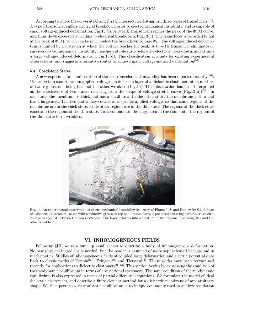
5.4. Coexistent States

A new experimental manifestation of the electromechanical instability has been reported recently[30].Under certain conditions, an applied voltage can deform a layer of a dielectric elastomer into a mixtureof two regions, one being flat and the other wrinkled (Fig.14). This observation has been interpretedas the coexistence of two states, resulting from the shape of voltage-stretch curve (Fig.13(a))[39]. Inone state, the membrane is thick and has a small area. In the other state, the membrane is thin andhas a large area. The two states may coexist at a specific applied voltage, so that some regions of themembrane are in the thick state, while other regions are in the thin state. The regions of the thick stateconstrain the regions of the thin state. To accommodate the large area in the thin state, the regions ofthe thin state form wrinkles.

Fig. 14. An experimental observation of electromechanical instability (courtesy of Plante J. S. and Dubowsky S.). A layerof a dielectric elastomer, coated with conductive grease on top and bottom faces, is pre-stretched using a frame. An electricvoltage is applied between the two electrodes. The layer deforms into a mixture of two regions, one being flat and theother wrinkled.

VI. INHOMOGENEOUS FIELDSFollowing §III, we now sum up small pieces to describe a body of inhomogeneous deformation.

No new physical ingredient is needed, but the reader is assumed of more sophisticated background inmathematics. Studies of inhomogeneous fields of coupled large deformation and electric potential dateback to classic works of Toupin[69], Eringen[70] and Tiersten[71]. These works have been reexaminedrecently for applications to dielectric elastomers[9–13]. This section begins by expressing the condition ofthermodynamic equilibrium in terms of a variational statement. The same condition of thermodynamicequilibrium is also expressed in terms of partial differential equations. We formulate the model of idealdielectric elastomers, and describe a finite element method for a dielectric membrane of any arbitraryshape. We then perturb a state of static equilibrium, a technique commonly used to analyze oscillation


and bifurcation. We conclude with a discussion of coexistent phases.

6.1. Variational Statement of Thermodynamic Equilibrium

A body of an elastic dielectric is represented by a sum of many small pieces, called material particles.Each material particle is named after the coordinate X of its place when the body is in a referencestate. In the current state, at time t, the particle X moves to a place with coordinate x. The function

x = x (X, t) (71)

describes the history of the deformation of the body. Define the deformation gradient F as

FiK =∂xi (X, t)

∂XK(72)

The deformation gradient generalizes the notion of the stretches.In the current state at time t, the electric potential at particle X is denoted as

Φ = Φ (X, t) (73)

The gradient of the electric potential defines the nominal electric field E, namely,

EK = −∂Φ (X, t)

∂XK(74)

The negative sign in Eq.(74) follows the convention that the electric field points from a material particleof a high voltage to a material particle of a low voltage.

Motivated by Eq.(22), we write the variation of the nominal density of the Helmholtz free energy,δW , in the form

δW = siKδFiK + EKδDK (75)

where δFiK is a small change in the deformation gradient, and δDK is a small change in the nominalelectric displacement. Equation (75) defines the nominal stress s as a tensor work-conjugate to thedeformation gradient F , and the nominal electric displacement D as a vector work-conjugate to thenominal electric field E.

Inspecting Eqs.(72) and (74), we wish to use the deformation gradient and the nominal electric fieldas the independent variables. Introducing a new quantity W by

W = W − EKDK (76)

The quantity W may be called the electrical Gibbs free energy. A combination of Eqs.(75) and (76)gives

δW = siKδFiK − DKδEK (77)

We may call the quantity DKδEK the complementary electrical work.

A material model is prescribed by a function W = W(

F , E)

. When the body undergoes a rigid-body

motion, the free energy is invariant. Consequently, the function depends on the deformation gradientF through the Green deformation tensor, CKL = FiKFiL. Associated with small changes δFiK andδEK , the electrical Gibbs free energy changes by

δW =∂W

(

F , E)

∂FiKδFiK +

∂W(

F , E)

∂EK

δEK (78)

On each material element of volume dV (X), we prescribe mass ρ (X) dV , force B (X, t) dV andcharge q (X, t) dV . The effect of inertia may be represented by adding to the force the inertial force, so thatthe combination of the applied force and the inertial force on the element of volume is

(

B − ρ∂2x/∂t2

)

dV .The body may consist of dissimilar dielectrics and conductors, separated by interfaces. Consider aninterface separating two parts of the body labeled as − and +. When the body is in the reference state,denote an element of the interface by dA (X), and denote the unit vector normal to the element of the


interface by N , pointing toward part +. On the element of the interface, we prescribe force T (X, t) dAand charge ω (X , t) dA.

Let δxi = ξi (X) be a field of virtual displacement of the body. Associated with the field of virtualdisplacement, the forces do virtual work

∫ (

Bi − ρ∂2xi/∂t2)

δxidV +∫

TiδxidA. Similarly, let δΦ =η (X) be a field of virtual electric potential of the body. Associated with the field of electric potential,the charges do virtual complementary work

∫

qδΦdV +∫

ωδΦdA. The virtual deformation gradient is

δFiK = ∂ξi (X) /∂XK , and the virtual nominal electric field is δEK = −∂η (X) /∂XK . The virtualchange in the electrical Gibbs free energy is

∫

δWdV , where δW is given by Eq.(78).When the body is in thermodynamic equilibrium, the change in the electrical Gibbs free energy

equals the mechanical work minus the complementary electrical work:∫

δWdV =

∫(

Bi − ρ∂2xi

∂t2

)

δxidV +

∫

TiδxidA −

∫

qδΦdV −

∫

ωδΦdA (79)

This condition of thermodynamic equilibrium has the similar physical content as Eqs.(1) and (21), andholds for arbitrary and independent variations δx and δΦ. The above presentation follows closely aprevious paper[12]. Variational statements of various forms may be developed from alternative startingpoints[72–75].

Once the loads and the electrical Gibbs free-energy function W(

F , E)

are prescribed, the varia-

tional statement (79), along with the definitions (72) and (74), is the basis for the finite element method,determining the field of deformation x (X, t) and the field of electric potential Φ (X, t) simultaneously.Several implementations of the finite element method have been reported[75–78], but few practical ex-amples are available. Significant effort is needed to develop the finite element method, and to apply themethod to analyze phenomena and devices.

6.2. Differential Equations

A comparison of Eqs.(77) and (78) gives that

siK =∂W

(

F , E)

∂FiK(80)

DK = −∂W

(

F , E)

∂EK

(81)

Once the electrical free-energy function W(

F , E)

is prescribed, Eqs.(80) and (81) constitute the

equations of state.Inserting Eqs.(72), (74) and (77) into the condition of thermodynamic equilibrium (79), and recalling

that the condition holds for arbitrary and independent variations in δx and δΦ, we obtain that

∂siK (X, t)

∂XK+ Bi (X , t) = ρ (X)

∂2xi (X, t)

∂t2(82)

in the volume(

s−iK − s+iK

)

NK = Ti (83)

on the interfaces∂DK (X, t)

∂XK= q (X, t) (84)

in the volume, and(

D+K − D−

K

)

NK = ω (X, t) (85)

on the interfaces. Equations (82) and (83) reproduce the equations for momentum balance, and Eqs.(84)and (85) reproduce Gauss’s law of electrostatics.

Equations (71)-(74) and (80)-(85) are governing equations to determine the field of deformationx (X, t) and the field of electric potential Φ (X, t) simultaneously, once the loads and the free-energy


function W(

F , E)

are prescribed. These partial differential equations have been used to solve boundary-

value problems[79–86]. Observe that the equations of mechanics, (71), (72), (82) and (83), decouple fromthose of electrostatics, (73), (74), (84) and (85). The only coupling between mechanics and electrostaticsarises from the material model, (80) and (81).

6.3. True Quantities

The true stress σij relates to the nominal stress by

σij =FjK

detFsiK (86)

The true electric displacement Di relates to the nominal electric displacement as

Di =FiK

detFDK (87)

The true electric field Ei relates to the nominal electric field as

Ei = HiKEK (88)

where HiK is the inverse of the deformation gradient, namely, HiKFiL = δKL and HiKFjK = δij .The true quantities may be taken as functions of x and t, and satisfy the familiar partial differentialequations in mechanics and electrostatics.

6.4. Ideal Dielectric Elastomers

For an isotropic elastic dielectric, the free-energy density is a function of six invariants of thedeformation gradient tensor and the electric field vector[69]. Function of this complexity is unavailablefor any real material. We next describe ideal dielectric elastomers—a material model nearly exclusivelyused in the literature. As discussed before in connection with Fig.9, for an ideal dielectric elastomer,the dielectric behavior is the same as that of a liquid—that is, the dielectric behavior is unaffected bydeformation[39].

As a simplest model of a dielectric liquid, assume that the true electric displacement Dm is linearin the true electric field Em:

Dm = εEm (89)

The permittivity ε is taken to be independent of deformation.Using Eqs.(87) and (88), we express Eq.(89) in terms of the nominal fields:

DN = εELHmNHmL det F (90)

Inserting Eq.(90) into Eq.(81) and integrating with respect to E while holding F fixed, we obtain thenominal density of the electrical Gibbs free energy:

W(

F , E)

= Ws (F ) −ε

2EN ELHmNHmL detF (91)

The constant of integration, Ws (F ), is the free energy associated with the elasticity of the elastomer,which may be selected from a large menu in the theory of elasticity. While the elastomer is nearlyincompressible, in the finite element method, it is convenient to allow the material to be compressiblewith a large bulk modulus.

Insert Eq.(91) into Eq.(80), and recall mathematical identities ∂HmN/∂FiK = −HmKHiN and∂ detF /∂FiK = HiK detF . We obtain that

siK =∂Ws (F )

∂FiK+ εEN EL

(

HiNHmKHmL −1

2HmNHmLHiK

)

detF (92)

This equation of state relates the nominal stress to the deformation gradient and the nominal electricfield.


A combination of Eqs.(86) and (92) gives

σij =FjK

detF

∂Ws (F )

∂FiK+ ε

(

EiEj −1

2EmEmδij

)

(93)

This equation relates the true stress to the deformation gradient and the true electric field. The con-tribution due to the deformation gradient results from the stretching of the elastomer, and is thesame as that in the theory of elasticity. The contribution due to the electric field is identical to thatderived by Maxwell[40]. When σij = 0, Eq.(93) balances elasticity and electrostatics, and determinesthe voltage-induced deformation. As commented before, the Maxwell stress correctly accounts for thevoltage-induced deformation only when the dielectric behavior is liquid-like, an idealization that workswell with elastomers, but not for other solid dielectrics.

Equations (89) and (93) constitute the equations of state, for an ideal dielectric elastomer, in termsof the true quantities. The equations of state exhibit one-way coupling: the deformation does not affectthe electrical behavior, but the electric field contributes to the stress-stretch relation. As noted before,the partial differential equations of mechanics decouple from those of electrostatics. One may solveelectrostatic boundary-value problems in terms of the true fields, and then add the Maxwell stress insolving the elastic field. Of course, the deformation will change the shape of the boundary of the body.This change must be included in solving the electrostatic problems. The one-way coupling may notbring any advantage after all.

The model of ideal dielectric elastomers can be generalized to account for nonlinear dielectric behavior,by replacing Eq.(89) with a nonlinear relation between the electric field and electric displacement[12,48].Furthermore, the model of ideal dielectric elastomers can be modified to include dissipative processes,such as viscoelasticity, dielectric relaxation, and electrical conduction[21,52].

6.5. Weak Statements

We recall a well known statement in continuum mechanics. On each part of the boundary of a body,either the displacement or the traction is prescribed. Let ξi (X) be a function defined in the body andon the boundary. Set ξi (X) = 0 on the part of the boundary where the displacement is prescribed, butleave the function ξi (X) otherwise arbitrary. Equations (82) and (83) are equivalent to requiring that

∫

siK∂ξi

∂XKdV =

∫(

Bi − ρ∂2xi

∂t2

)

ξidV +

∫

TiξidA (94)

hold for any arbitrary function ξi (X) as described above. The volumetric integrals extend over thevolume of the body, and the surface integral extends over the boundary where the traction is prescribed.The statement (94) is readily confirmed by applying the divergence theorem.

Also recall a weak statement concerning electrostatics. On each part of the boundary, either theelectric potential or the charge is prescribed. Let η (X) be a function defined in the body and on theboundary. Set η (X) = 0 on the part of the boundary where the electric potential is prescribed, andleave η (X) otherwise arbitrary. Equations (84) and (85) are equivalent to requiring that

∫(

−∂η

∂XK

)

DKdV =

∫

ηqdV +

∫

ηωdA (95)

hold for any arbitrary functions η (X) as specified above. The volumetric integrals extend over thevolume, and the surface integral extends over the boundary where charge is prescribed.

6.6. Finite Element Method for an Elastic Dielectric Membrane

To induce a significant deformation, the voltage needs to be on the order Φ ∼ H√

µ/ε, whereH is the thickness over which the voltage is applied, µ the shear modulus, and ε the permittivity. Arepresentative order of magnitude is

√

µ/ε ∼ 108 V/m, which is a very high electric field. Consequently,to reduce the voltage needed for actuation, nearly all dielectric elastomer transducers are in the formof thin membranes, with the thickness much smaller than the in-plane dimensions of the membranes.

Membranes of circular, spherical and axisymmetric symmetries have been analyzed[9,30,47,80–85].Here we briefly review a finite element method for dielectric membranes of arbitrary shapes, coupledwith passive materials of arbitrary shapes[77].


Consider a dielectric membrane sandwiched between two electrodes. The nominal electric field inthe membrane takes the form

E =Φ

H (X)N (X) (96)

where Φ is the voltage applied between the electrodes, H (X) is the thickness of the membrane, andN (X) is the unit vector normal to the membrane. Both the thickness and the unit normal vector aremeasured when the membrane is in the reference state, where the thickness may vary from place toplace, and the shape of the membrane can be curved. When the voltage Φ is prescribed, Eq.(96) givesthe nominal electric field E.

For any material specified by a function W(

F , E)

, the nominal stress relates to the deforma-

tion gradient and the nominal electric field by siK = ∂W(

F , E)

/∂FiK . This equation, along with

Eq.(96), relates the nominal stress to the deformation gradient, with Φ as a known parameter. The weakstatement (94) defines a boundary-value problem in elasticity. This boundary-value problem is readilyimplemented in the commercial finite element package ABAQUS by using a user-defined subroutine[77].ABAQUS readily accounts for passive materials of arbitrary shapes.

6.7. Linear Perturbation around a State of Static Equilibrium

We now return to the general theory in §6.1 and §6.2. Subject to a set of time-independent loads,a body may attain a state of static equilibrium. We may perturb this state with fields small in strainand electric field[12,67,68]. Such a linear perturbation analysis is commonly used to analyze oscillationand bifurcation[87].

Perturb the state of static equilibrium with a small-amplitude oscillation of frequency Ω. Write thetime-dependent fields of deformation and electric potential as

x (X, t) = x (X) + x

′ (X) exp (iΩt) (97)

Φ (X, t) = Φ (X) + Φ′ (X) exp (iΩt) (98)

where x (X) and Φ (X) are the state of static equilibrium, and x

′ (X) and Φ′ (X) are the amplitudefields of the oscillation. Associated with the static state of equilibrium, the deformation gradient isF

iK = ∂x

i (X) /∂XK , and the nominal electric field is E

K = −∂Φ (X) /∂XK . Associated with theoscillation, the amplitudes of the deformation gradient and the nominal electric field are

F ′

iK =∂x′

i (X)

∂XK(99)

E′

K = −∂Φ′ (X)

∂XK(100)

The amplitudes of the oscillation are small, so that the amplitudes of the nominal stress and thenominal electric displacement can be obtained by linear perturbation:

s′iK = KiKjLF ′

jL − eiKLE′

L (101)

D′

L = eiKLF ′

iK + εLKE′

K (102)

The tangent moduli are calculated from

KiKjL =∂2W

∂FjL∂FiK, εKL = −

∂2W

∂EK∂EL

, eiKL = −∂2W

∂FiK∂EL

(103)

The derivatives are calculated at the static field(

F, E

)

. So long as the oscillation around a static

field is concerned, all dielectrics, including vacuum, act like a linear piezoelectric. Because the staticstate of equilibrium can be inhomogeneous, the tangent moduli may vary from one material particleto another.


The amplitude fields satisfy the partial differential equations and boundary conditions:

∂s′iK∂XK

= −ρΩ2x′

i (104)

∂D′

K

∂XK= 0 (105)

(

s′−iK − s′+iK)

NK = 0 (106)

(

D′+K − D′−

K

)

NK = 0 (107)

The governing equations for the oscillation constitute an eigenvalues problem, with the frequency asthe eigenvalue.

Applying the weak statements (94) and (95) to the amplitude fields, we obtain that∫

s′iKF ′

iKdV = Ω2

∫

ρx′

ix′

idV (108)

∫

E′KD′

KdV = 0 (109)

Adding these two equations, and using Eqs.(101) and (102), we obtain that∫

(

KiKjLF ′

iKF ′

jL + εKLE′KE′

L

)

dV = Ω2

∫

ρx′

ix′

idV (110)

When the tangent moduli KiKjL and εKL are positive-definite, the frequency Ω is real-valued.Several oscillatory dielectric elastomer actuators have been analyzed[82,83]. The above analysis also

applies when the frequency is set to be zero. Equations (97) and (98) then pose a bifurcation problem:in the neighborhood of a given state of static equilibrium we look for other states of static equilibrium.This bifurcation problem has been discussed briefly in connection with the electromechanical instabilityin §V. More detailed discussions are available elsewhere[67,68].

6.8. Coexistent Phases

As noted in §V, coexistent phases have been observed experimentally for dielectric elastomers. Suchcoexistence has been analyzed by matching regions of two homogeneous states[39,88], and the transitionalregion has been analyzed by using finite element method[76]. Here we consider coexistent phases ingeneral terms. The displacement and electric potential are continuous across the phase boundary, butthe deformation gradient, stress, electric field and electric displacement can be discontinuous across thephase boundary. We next derive the conditions of equilibrium following an established method[89–91].

The elastomer, the applied forces and the applied charge together constitute a thermodynamicsystem. The free energy of the system includes contributions from all the parts:

G =

∫

WdV −

∫

BixidV −

∫

TixidA +

∫

ΦqdV +

∫

ΦωdA (111)

The free energy varies when the displacement and electric potential vary, and when the phase boundarymoves. In equilibrium, the variation of the free energy associated with any such change must vanish.

§6.1 has considered the variation of the free energy associated with the variations of deformationand electric potential, while holding the phase boundary immobile. Setting this variation of free energyto zero, Eq.(79), we obtain field equations in §6.2. In particular, consider an element of the phaseboundary dA (X), with N (X) being the unit vector normal to the element. Equation (83) requiresthat the traction be continuous across the phase boundary:

〈siK〉NK = 0 (112)

The notation 〈f〉 stands for the jump of f across the phase boundary. Similarly, Eq.(85) requires thatthe component of the electric displacement normal to the phase boundary be continuous across thephase boundary:

⟨

DK

⟩

NK = 0 (113)


We next consider the change in the free energy associated with the motion of the phase boundary.The motion of the phase boundary is tracked in the reference state. When the phase boundary movesby a displacement δα (X), the element of the phase boundary at material particle X moves to a newmaterial particle X + N (X) δα (X). Associated with the movement of the phase boundary, the freeenergy varies by

δG =

∫

⟨

W +(

DKEL − siKFiL

)

NKNL

⟩

δαdA (114)

The integral extends over the phase boundary. Equation (114) corrects a mistake in Eq.(4.22) in myprevious paper[91].

When the two phases are in equilibrium, δG vanishes for arbitrary small movement of the phaseboundary δα (X), so that the jump in front of δα (X) in Eq.(114) vanishes:

⟨

W +(

DKEL − siKFiL

)

NKNL

⟩

= 0 (115)

One can readily confirm that Eq.(115) recovers the condition for coexistence for a special case[39].

VII. CONCLUDING REMARKSA large number of examples in biology demonstrate that deformation of soft materials connect

many stimuli to many functions essential to life. Using soft active materials to create soft machines hasemerged as an exciting field of engineering. To participate in advancing the field of soft active materialsand soft machines effectively, mechanicians must retool our laboratories and our software, as well asadapt our theories. While theories are being developed for diverse soft active materials, this reviewfocuses on one class of soft active materials: dielectric elastomers. This focus allows us to review thetheory of dielectric elastomers in some depth, within the framework of nonlinear continuum mechanicsand nonequilibrium thermodynamics, while motivating the theory by empirical observations, molecularpictures and applications. It is hoped that the theory will be used to develop software, study intriguingphenomena of electromechanical coupling, and aid the design of electromechanical transducers. It isalso hoped that this review of dielectric elastomers will contribute to the rapid development of theoriesfor diverse soft active materials and soft machines.

References[1] Mathger,L.M., Denton,E.J., Marshall,N.J. and Hanlon,R.T., Mechanisms and behavioral functions of struc-

tural coloration in cephalopods. Journal of the Royal Society Interface, 2008, 6 (Suppl 2): S149-S163.[2] Zwieniecki,M.A., Melcher,P.J. and Holbrook,N.M., Hydrogel control of xylem hydraulic resistance in plants.

Science, 2001, 291: 1059-1062.[3] Pelrine,R., Kornbluh,R., Pei,Q.B. and Joseph,J., High-speed electrically actuated elastomers with strain

greater than 100%. Science, 2000, 287: 836-839.[4] McKay,T., O’Brien,B., Calius,E. and Anderson,I., Self-priming dielectric elastomer generators. Smart Ma-

terials and Structures, 2010, 19: 055025.[5] Beebe,D.J., Moore,J.S., Bauer,J.M., Yu,Q., Liu,R.H., Devadoss,C. and Jo,B.H., Functional hydrogel struc-

tures for autonomous flow control inside microfluidic channels. Nature, 2000, 404: 588-590.[6] Calvert,P., Hydrogels for soft machines. Advanced Materials, 2009, 21: 743-756.[7] Trivedi,D., Rahn,C.D., Kier,W.M. and Walker,I.D., Soft robotics: biological inspiration, state of the art,

and future research. Applied Bionics and Biomechanics, 2008, 5: 99-117.[8] Cai,S.Q., Lou,Y.C., Ganguly,P., Robisson,A. and Suo,Z.G., Force generated by a swelling elastomer subject

to constraint. Journal of Applied Physics, 2010, 107: 103535.[9] Goulbourne,N.C., Mockensturm,E.M. and Frecker,M., A nonlinear model for dielectric elastomer mem-

branes, Journal of Applied Mechanics, 2005, 72: 899-906.[10] Dorfmann,A. and Ogden,R.W., Nonlinear electroelasticity. Acta Mechanica, 2005, 174: 167-183.[11] McMeeking,R.M. and Landis,C.M., Electrostatic forces and stored energy for deformable dielectric mate-

rials. Journal of Applied Mechanics, 2005, 72: 581-590.[12] Suo,Z.G., Zhao,X.H. and Greene,W.H., A nonlinear field theory of deformable dielectrics. Journal of the

Mechanics and Physics of Solids, 2008, 56: 467-286.[13] Trimarco,C., On the Lagrangian electrostatics of elastic solids. Acta Mechanica, 2009, 204: 193-201.[14] Sekimoto,K., Thermodynamics and hydrodynamics of chemical gels. Journal of Physics II, 1991, 1: 19-36.


[15] Dolbow,J., Fried,E. and Jia,H.D., Chemically induced swelling of hydrogels. Journal of the Mechanics and

Physics of Solids, 2004, 52: 51-84.[16] Baek,S. and Srinivasa,A.R., Diffusion of a fluid through an elastic solid undergoing large deformation.

International Journal of Non-linear Mechanics, 2004, 39: 201-218.[17] Hong,W., Zhao,X.H., Zhou,J.X. and Suo,Z.G., A theory of coupled diffusion and large deformation in

polymeric gels. Journal of the Mechanics and Physics of Solids, 2008, 56: 1779-1793.[18] Doi,M., Gel dynamics. Journal of the Physical Society of Japan, 2009, 78: 052001.[19] Chester,S.A. and Anand,L., A coupled theory of fluid permeation and large deformations for elastomeric

materials. Journal of the Mechanics and Physics of Solids, 2010, 58: 1879-1906.[20] Nemat-Nasser,S. and Li,J.Y., Electromechanical response of ionic polymer-metal composites. Journal of

Applied Physics, 2000, 87: 3321-3331.[21] Hong,W., Zhao,X.H. and Suo,Z.G., Large deformation and electrochemistry of polyelectrolyte gels. Journal

of the Mechanics and Physics of Solids, 2010, 58: 558-577.[22] Baek,S. and Srinivasa,A.R., Modeling of the pH-sensitive behavior of an ionic gel in the presence of diffusion.

International Journal of Non-linear Mechanics, 2004, 39: 1301-1318.[23] Li,H., Luo,R., Birgersson,E. and Lam,K.Y., Modeling of multiphase smart hydrogels responding to pH and

electric voltage coupled stimuli. Journal of Applied Physics, 2007, 101: 114905.[24] Marcombe,R., Cai,S.Q., Hong,W., Zhao,X.H., Lapusta,Y. and Suo,Z.G., A theory of constrained swelling

of a pH-sensitive hydrogel. Soft Matter, 2010, 6: 784-793.[25] Cai,S.Q. and Suo,Z.G., Mechanics and chemical thermodynamics of a temperature-sensitive hydrogel.

Manuscript in preparation.[26] Shankar,R., Ghosh,T.K. and Spontak,R.J., Dielectric elastomers as next-generation polymeric actuators.

Soft Matter, 2007, 3: 1116-1129.[27] Carpi,F., Electromechanically active polymers, editorial introducing a special issue dedicated to dielectric

elastomers. Polymer International, 2010, 59:277-278.[28] Brochu,P. and Pei,Q.B., Advances in dielectric elastomers for actuators and artificial muscles. Macromolec-

ular Rapid Communications, 2010, 31: 10-36.[29] Gibbs,J.W., Graphical methods in the thermodynamics of fluids. Transactions of the Connecticut Academy,

1973, 2: 309-342 (Available online at Google Books).[30] Plante,J.S. and Dubowsky,S., Large-scale failure modes of dielectric elastomer actuators. International

Journal of Solids and Structures, 2006, 43: 7727-7751.[31] Wissler,M. and Mazza,E., Mechanical behavior of acrylic elastomer used in dielectric elastomer actuators.

Sensors and Actuators A, 2007, 134: 494-504.[32] Kollosche,M. and Kofod,G., Electrical failure in blends of chemically identical, soft thermoplastic elastomers

with different elastic stiffness. Applied Physics Letters, 2010, 96: 071904.[33] Lochmatter,P., Kovacs,G. and Michel,S., Characterization of dielectric elastomer actuators based on a

hyperelastic film model. Sensors and Actuators A, 2007, 135: 748-757.[34] Moscardo,M., Zhao,X.H., Suo,Z.G. and Lapusta,Y., On designing dielectric elastomer actuators. Journal

of Applied Physics, 2008, 104: 093503.[35] Koh,S.J.A., Zhao,X.H. and Suo,Z.G., Maximal energy that can be converted by a dielectric elastomer

generator. Applied Physics Letters, 2009, 94: 262902.[36] Koh,S.J.A., Keplinger,C., Li,T.F., Bauer,S. and Suo,Z.G., Dielectric elastomer generators: how much energy

can be converted? Transactions on Mechatronics, in press.[37] Diaz-Calleja.,R. and Llovera-Segovia,P., Energy diagrams and stability restrictions for electroelastic gen-

erators. Journal of Polymer Science B, 2010, 48: 2023-2028.[38] Gibbs,J.W., A method of geometrical representation of the thermodynamic properties of substances by

means of surfaces. Transactions of the Connecticut Academy, 1973, 2: 382-404 (Available online at GoogleBooks).

[39] Zhao,X.H., Hong,W. and Suo,Z.G., Electromechanical coexistent states and hysteresis in dielectric elas-tomers. Physical Review B, 2007, 76: 134113.

[40] Maxwell,J.C., A Treatise on Electricity and Magnetism, Volume 1, Chapter V, Mechanical action betweentwo electrical systems. Oxford: Oxford University Press, 1873 (Available online at Google Books).

[41] Kofod,G., Sommer-Larsen,P., Kornbluh,R. and Pelrine,R., Actuation response of polyacrylate dielectricelastomers. Journal of Intelligent Material Systems and Structures, 2003, 14: 787-793.

[42] Kofod,G. and Sommer-Larsen,P., Silicone dielectric elastomer actuators: finite-elasticity model of actuation.Sensors and Actuators A, 2005, 122: 273-283.

[43] Treloar,L.R.G., The Physics of Rubber Elasticity. Oxford: Oxford University Press, 1975.[44] Arruda,E.M. and Boyce,M.C., A three-dimensional constitutive model for the large stretch behavior of

rubber elastic materials. Journal of the Mechanics and Physics of Solids, 1993, 41: 389-412.


[45] Gent,A.N., A new constitutive relation for rubber. Rubber Chemistry and Technology, 1996, 69: 59-61.

[46] Zhao,X. and Suo,Z.G., Electrostriction in elastic dielectrics undergoing large deformation. Journal of Ap-

plied Physics, 2008, 104: 123530.

[47] Wissler,M. and Mazza,E., Electromechanical coupling in dielectric elastomer actuators. Sensors and Ac-

tuators A, 2007, 138: 384-393.

[48] Li,B., Liu,L.W. and Suo,Z.G., Extension limit, polarization saturation, and snap-through instability ofdielectric elastomers. Submitted for publication.

[49] Lochmatter,P., Kovacs,G. and Wissler,M., Characterization of dielectric elastomers based on a visco-hyperelastic film model. Smart Materials and Structures, 2007, 135: 748-757.

[50] Ha,S.M., Wissler,M., Pelrine,R., Stanford,S., Kovas,G. and Pei,Q., Characterization of electroelastomersbased on interpenetrating polymer networks. Proceedings of SPIE, 2007, 6524: 652408.

[51] Plante,J.S. and Dubowsky,S., On the performance mechanisms of dielectric elastomer actuators. Sensors

and Actuators A, 2007, 137: 96-109.

[52] Zhao,X.H., Koh,S.J.A. and Suo,Z.G., Nonequilibrium thermodynamics of dielectric elastomers. Interna-

tional Journal of Applied Mechanics. Preprint: http://www.seas.harvard.edu/suo/papers/242.pdf.

[53] Silberstein,M.N. and Boyce,M.C., Constitutive modeling of the rate, temperature, and hydration dependentdeformation response of Nafion to monotonic and cyclic loading. Journal of Power Sources, 2010, 195: 5692-5706.

[54] Zhang,Q.M., Bharti,V. and Zhao,X., Giant electrostriction and relaxor ferroelectric behavior in electron-irradiated poly (vinylidene fluoride-trifluoroethylene) copolymer. Science, 1998, 280: 2101-2104.

[55] Pelrine,R.E., Kornbluh,R.D. and Joseph,J.P., Electrostriction of polymer dielectrics with compliant elec-trodes as a means of actuation. Sensors and Actuators A, 1998, 64: 77-85.

[56] Ha,S.M., Yuan,W., Pei,Q.B., Pelrine,R. and Stanford,S., Interpenetrating polymer networks for high-performance electroelastomer artificial muscles. Advanced Materials, 2006, 18: 887-891.

[57] Suo,Z.G. and Zhu,J., Dielectric elastomers of interpenetrating networks. Applied Physics Letters, 2009, 95:232909.

[58] Shankar,R., Ghosh,T.K. and Spontak,R.J., Electroactive nanostructured polymers as tunable actuators.Advanced Materials, 2007, 19: 2218-2223.

[59] Keplinger,C., Kaltenbrunner,M., Arnold,N. and Bauer,S., Rontgen’s electrode-free elastomer actuatorswithout electromechanical pull-in instability. PNAS, 2010, 107: 4505-4510.

[60] Stark,K.H. and Garton,C.G., Electric strength of irradiated polythene. Nature, 1955, 176: 1225-1226.

[61] Zhao,X.H. and Suo,Z.G., Theory of dielectric elastomers capable of giant deformation of actuation. Physical

Review Letters, 2010, 104: 178302.

[62] Zhao,X.H. and Suo,Z.G., Method to analyze electromechanical stability of dielectric elastomers. Applied

Physics Letters, 2007, 91: 061921.[63] Norris,A.N., Comments on ‘Method to analyze electromechanical stability of dielectric elastomers’. Applied

Physics Letters, 2008, 92: 026101.[64] Diaz-Calleja,R., Riande,E. and Sanchis,M.J., On electromechanical stability of dielectric elastomers. Ap-

plied Physics Letters, 2008, 93: 101902.

[65] Leng,J.S., Liu,L.W., Liu,Y.J., Yu,K. and Sun,S.H., Electromechanical stability of dielectric elastomers.Applied Physics Letters, 2009, 94: 211901.

[66] Xu,B.X., Mueller,R., Classen,M. and Gross,D., On electromechanical stability analysis of dielectric elas-tomer actuators. Applied Physics Letters, 2010, 97: 162908.

[67] Dorfmann,A. and Ogden,R.W., Nonlinear electroelastics: incremental equations and stability. International

Journal of Engineering Science, 2010, 48: 1-14.[68] Bertoldi,K. and Gei,M., Instabilities in multilayered soft dielectrics. Journal of the Mechanics and Physics

of Solids, 2011, 59: 18-42.

[69] Toupin,R.A., The elastic dielectric. Journal of Rational Mechanics and Analysis, 1956, 5: 849-914.

[70] Eringen,A.C., On the foundations of electroelastostatics. International Journal of Engineering Science,1963, 1: 127-153.

[71] Tiersten,H.F., On the nonlinear equations of thermoelectroelasticity. International Journal of Engineering

Science, 1971, 9: 587-604.[72] McMeeking,R.M., Landis,C.M. and Jiminez,M.A., A principle of virtual work for comined electrostatic and

mechanical loading of materials. International Journal of Non-Linear Mechanics, 2007, 42: 831-838.[73] Bustamente,R., Dorfmann,A. and Ogden,R.W., Nonlinear electroelastostatics: a variational framework.

Zeitschrift fur Angewandte Mathematik und Physik, 2009, 60: 154-177.

[74] Trimarco,C., On the dynamics of electromagnetic bodies. International Journal of Advances in Engineering

Sciences and Applied Mathematics, 2009, 1: 157-162.


[75] Vu,D.K., Steinmann,P. and Possart,G., Numerical modelling of non-linear electroelasticity. International

Journal for Numerical Methods in Engineering, 2007, 70: 685-704.[76] Zhou,J.X., Hong,W., Zhao,X.H. and Suo,Z.G., Propagation of instability in dielectric elastomers. Interna-

tional Journal of Solids and Structures, 2008, 45: 3739-3750.[77] Zhao,X.H. and Suo,Z. G., Method to analyze programmable deformation of dielectric elastomer layers.

Applied Physics Letters, 2008, 93: 251902. The user-supplied subroutine for ABAQUS is available athttp://imechanica.org/node/4234.

[78] O’Brien,B., McKay,T., Calius,E., Xie,S. and I.Anderson, Finite element modelling of dielectric elastomerminimum energy structures. Applied Physics A, 2009, 94: 507-514.

[79] Dorfmann,A. and Ogden,R.W., Nonlinear electroelastic deformations. Journal of Elasticity, 2006, 82: 99-127.

[80] Mockensturm,E.M. and Goulbourne,N., Dynamic response of dielectric elastomers. International Journal

of Non-Linear Mechanics, 2006, 41: 388-395.[81] Goulbourne,N.C., Mockensturm,E.M. and Frecker,M.I., Electro-elastomers: large deformation analysis of

silicone membranes. International Journal of Solids and Structures, 2007, 44: 2609-2626.[82] Zhu,J., Cai,S.Q. and Suo,Z.G., Resonant behavior of a membrane of a dielectric elastomer. International

Journal of Solids and Structures, 2010, 47: 3254-3262.[83] Zhu,J., Cai,S.Q. and Suo,Z.G., Nonlinear oscillation of a dielectric elastomer balloon. Polymer International,

2010, 59: 378-383.[84] He,T.H., Zhao,X.H. and Suo,Z.G., Equilibrium and stability of dielectric elastomer membranes undergoing

inhomogeneous deformation. Journal of Applied Physics, 2009, 106: 083522.[85] He,T.H., Cui,L.L., Chen,C. and Suo,Z.G., Nonlinear deformation analysis of dielectric elastomer-spring

system. Smart Materials and Structures, 2010, 19: 085017.[86] Zhu,J., Stoyanov,H., Kofod,G. and Suo.Z.G., Large deformation and electromechanical instability of a

dielectric elastomer tube actuator. Journal of Applied Physics, 2010, 108: 074113.[87] Willis,J.R., Stability of Media and Structures. http://imechanica.org/node/9292.[88] De Tommasi,D., Puglisi,Saccomandi,G. and Zurlo,G., Pull-in and wrinkling instabilities of electroactive

dielectric actuators. Journal of Physics D, 2010, 43: 325501.[89] Eshelby,J.D., The continuum theory of lattice defects. Solid State Physics, 1956, 3: 79-144.[90] Abeyaratne,R. and Knowles,J.K., On the driving traction acting on a surface of strain discontinuity in a

continuum. Journal of the Mechanics and Physics of Solids, 1990, 38: 345-360.[91] Suo,Z.G., Motions of microscopic surfaces in materials. Advances in Applied Mechanics, 1997, 33: 193-294.

theory of dielectric

Documents