theory and practice of cavity rf test systemsuspas.fnal.gov/materials/11odu/rf_test.pdf · theory...
TRANSCRIPT
THEORY AND PRACTICE OF CAVITY RF TEST SYSTEMS *
Tom Powers†, Thomas Jefferson National Accelerator Facility
Abstract Over the years Jefferson Lab staff members have
performed about 2500 cold cavity tests on about 500
different superconducting cavities. Most of these cavities
were later installed in 73 different cryomodules, which
were used in three different accelerators. All of the
cavities were tested in our vertical test area. About 25%
of the cryomodules were tested in our cryomodule test
facility and later commissioned in an accelerator. The
remainder of the cryomodules were tested and
commissioned after they were installed in their respective
accelerator. This paper is an overview which should
provide a practical background in the RF systems used to
test the cavities as well as provide the mathematics
necessary to convert the raw pulsed or continuous wave
RF signals into useful information such as gradient,
quality factor, RF-heat loads and loaded Q’s.
Additionally, I will provide the equations necessary for
determining the measurement error associated with these
values.
RF SOURCE
There are two fundamental ways to provide a low level
RF (LLRF) drive signal to a cavity. In situations where
beam is involved, fixed frequency RF systems are
implemented. These make use of high gain phase and
amplitude control loops. In these systems the mechanical
length of the cavity is usually adjusted using tuners driven
by motors, piezo crystals, or both. [1, 2, 3] Some systems
make use of high power voltage controlled reactive tuners
to pull the cavity’s center frequency as seen at the
fundamental power port.[4] An integral part of these
LLRF systems is an interface to and algorithm for driving
the tuner mechanism.
The second way is to make use of a LLRF system
which is designed to track the cavity frequency. Such
systems have two major advantages. They can be used
with critically coupled SRF cavities, which have
bandwidths on the order of 1 Hz, and the cavities do not
need operational mechanical tuners. Thus, when there are
pressure variations or frequency shifts due to microphonic
or Lorentz effects, the LLRF system tracks the shifts and
the cavity gradient is maximized for the given forward
power and input coupling. Additionally, using such
systems allows one to intentionally vary the cavity
frequency so that the tuners can be fully characterized and
measurements of phenomena such as dynamic Lorentz
effects and microphonics can be studied [5]. The majority
of the cavity tests completed at Jefferson Lab were done
using voltage controlled oscillators configured in phase
locked loops (VCO-PLL).
The VCO-PLL
A detailed mathematical treatment of phase locked loop
circuits is provided in Reference [6]. The intent of this
work is to go trough the practical considerations relating
to VCO-PLLs when using them for driving supercon-
ducting cavities. Although these systems can be designed
to be compact and inexpensive by using surface mount
components and custom printed circuit boards, in most
instances connectorized components are used in order to
minimize the non-recurring design costs. All of the
devices described are generally available in both formats.
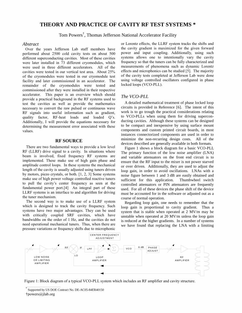
Figure 1 shows a block diagram for a basic VCO-PLL
The primary function of the low noise amplifier (LNA)
and variable attenuators on the front end circuit is to
ensure that the RF input to the mixer is not power starved
or over driven. Additionally, they are used to adjust the
loop gain, in order to avoid oscillations. LNAs with a
noise figure between 1 and 3 dB are easily obtained and
sufficient for this application. Thumbwheel switch
controlled attenuators or PIN attenuators are frequently
used. For all of these devices the phase shift of the device
must be accounted for in the software or adjusted out as a
course of normal operation.
Regarding loop gain, one needs to remember that the
loop gain is proportional to cavity gradient. Thus a
system that is stable when operated at 2 MV/m may be
unstable when operated at 20 MV/m unless the loop gain
is reduced at the higher gradients. In a number of systems
we have found that replacing the LNA with a limiting
Figure 1: Block diagram of a typical VCO-PLL system which includes an RF amplifier and cavity structure.
PH ASE
AD JU ST
R F
LO
IFLPF
C EN TER FR EQ U EN C Y
AD JU STM EN T
VC O 6 dB
LO O P
AM PLIF IER
R F
AM PLIF IER
LO W N O ISE
O R LIM ITIN G
AM PLIF IER
___________________________________________
* Supported by US DOE Contract No. DE-AC05-84ER40150
amplifier, such as the difficult to find Lucent LG1605,
provides an expanded dynamic range with reduced
oscillation problems.
The LNA section is followed by a mixer. Typically
double balanced diode ring mixers are used. Devices
such as a Mini-Circuits ZFM-150 are perfectly adequate.
The two major considerations are that the intermediate
frequency (IF) output must be DC coupled and the
operating level of the local oscillator (LO) should be as
high as practical. Typically 7 to 13 dBm mixers are used.
Mixers with a LO much higher than 13 dBm will require
that one insert an amplifier between the coupled VCO
output and the LO input.
The low pass filter (LPF) stage serves two purposes.
The first is to eliminate any the frequency content at the
fundamental frequency or it’s second harmonic. The
other purpose is to limit the loop bandwidth to about
20 kHz which reduces the system noise without
compromising the lock time necessary for cavities which
happen to have rise times on the order of 1 ms or less.
The variable gain amplifier provides another way to
adjust loop gain that, unlike the LNA, is independent of
loop phase. Unless the following phase shifter is capable
of more than 360º of phase shift, this amplifier should
have an invert switch. At the summing junction, the error
signal is summed with an offset signal, that is typically
generated using two ten-turn potentiometers, one for
coarse and one for fine frequency adjustments. The
reference voltage for the potentiometer is typically a band
gap voltage reference based circuit. This is done in order
to ensure that the source is stable and low noise. In
addition to custom circuit designs, devices like a Stanford
Research SR540 amplifier can be used to implement the
loop gain and filter functions.
There are a number of choices for VCOs. The least
expensive devices are broadband devices such as those
produced by Mini-Circuits. While they have the
advantage of low cost, they typically have electrical
tuning ranges between 500 MHz and 1000 MHz. With a
control voltage range between 10 and 25 Volts, these
devices have a tuning a sensitivity, between 30 MHz/V
and 100 MHz/V. Additionally, inexpensive devices are
not thermally stabilized and are subject to thermal drifts.
When excessive, these thermal drifts have been known to
cause a cavity – VCO-PLL system to lose lock within
minutes of being properly tuned. Such drifts can be
mitigated by packaging the devices in a thermally isolated
enclosure such as a foam lined metal box.
For a few thousand dollars one can purchase a custom
VCO that is thermally stabilized. Devices manufactured
by EMF Systems Inc., as well as others, can be
mechanically tuned over a range of a few hundred MHz
with an electrical tuning range and sensitivity on the order
of 10 MHz and 1 MHz/V respectively. [7] (Note: Tuning
sensitivities and ranges are given for VCOs operated
between 800 MHz and 2 GHz.)
Although expensive, an excellent alternative for the
VCO is to use an RF signal source that has an option for
an external frequency modulation (FM) control which can
be DC-coupled. Sources such as an Agilent E4422B
work well for this application. This and similar RF
sources have a low FM bandwidth, have stable low noise
RF drive capabilities, and are flexible with respect to the
operating frequency. They have an added advantage in
that the output can be AM modulated simultaneous with
FM modulation. This configuration is used when
performing a measurement of the dynamic Lorentz force
effects [5]. Remember when performing such tests that
the minimum RF amplitude must be maintained at the LO
port on the mixer for the system to function properly.
The final low level section consists of a directional
coupler, along with the amplitude and phase controls. The
directional coupler is used to provide the LO signal from
the VCO to the input of the mixer. The specific coupling
is determined by the output capability of the VCO and the
required LO signal level. In some cases an amplifier must
be used between the coupler and the mixer in order to
provide sufficient signal level. Typically the phase shifter
is a mechanical device such as a Narda 3752 or Arra
D3428B. When selecting these devices insure that they
provide at least 190º of phase shift or 370º depending on
the configuration of the loop amplifier. For manual
systems, a series of mechanical attenuators are used to
adjust the RF drive level.
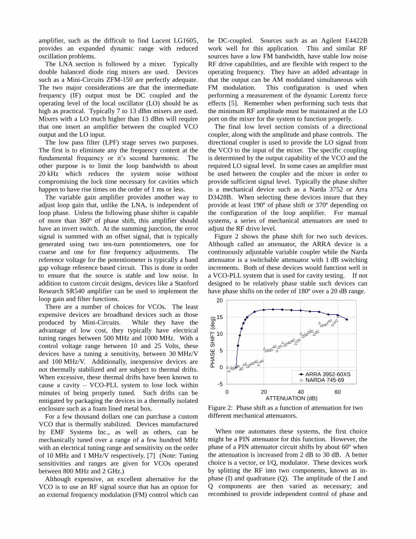
Figure 2 shows the phase shift for two such devices.
Although called an attenuator, the ARRA device is a
continuously adjustable variable coupler while the Narda
attenuator is a switchable attenuator with 1 dB switching
increments. Both of these devices would function well in
a VCO-PLL system that is used for cavity testing. If not
designed to be relatively phase stable such devices can
have phase shifts on the order of 180º over a 20 dB range.
-5
0
5
10
15
20
0 20 40 60ATTENUATION (dB)
PH
AS
E S
HIF
T (
deg)
ARRA 3952-60XSNARDA 745-69
Figure 2: Phase shift as a function of attenuation for two
different mechanical attenuators.
When one automates these systems, the first choice
might be a PIN attenuator for this function. However, the
phase of a PIN attenuator circuit shifts by about 60º when
the attenuation is increased from 2 dB to 30 dB. A better
choice is a vector, or I/Q, modulator. These devices work
by splitting the RF into two components, known as in-
phase (I) and quadrature (Q). The amplitude of the I and
Q components are then varied as necessary; and
recombined to provide independent control of phase and
amplitude of the RF. Discrete device I/Q modulators
which use analog voltage controls are produced by
companies like Analog Devices and Aligent Tech-
nologies. Connectorized devices with digital controls are
available from GT Microwave and Vectronics, Inc.
The RF amplifier shown in the diagram varies
depending on the loaded-Q of the cavity. For systems that
are near critical coupling, i. e. very little reflected power
at the input coupler, the amplifiers are usually solid state
devices typically on the order of a few hundred watts.
When the cavity is configured in a cryomodule they are
typically strongly over coupled and the amplifier is
typically a klystron delivering several kilowatts to several
hundred kilowatts of RF power.
VERTICAL TEST SYSTEM
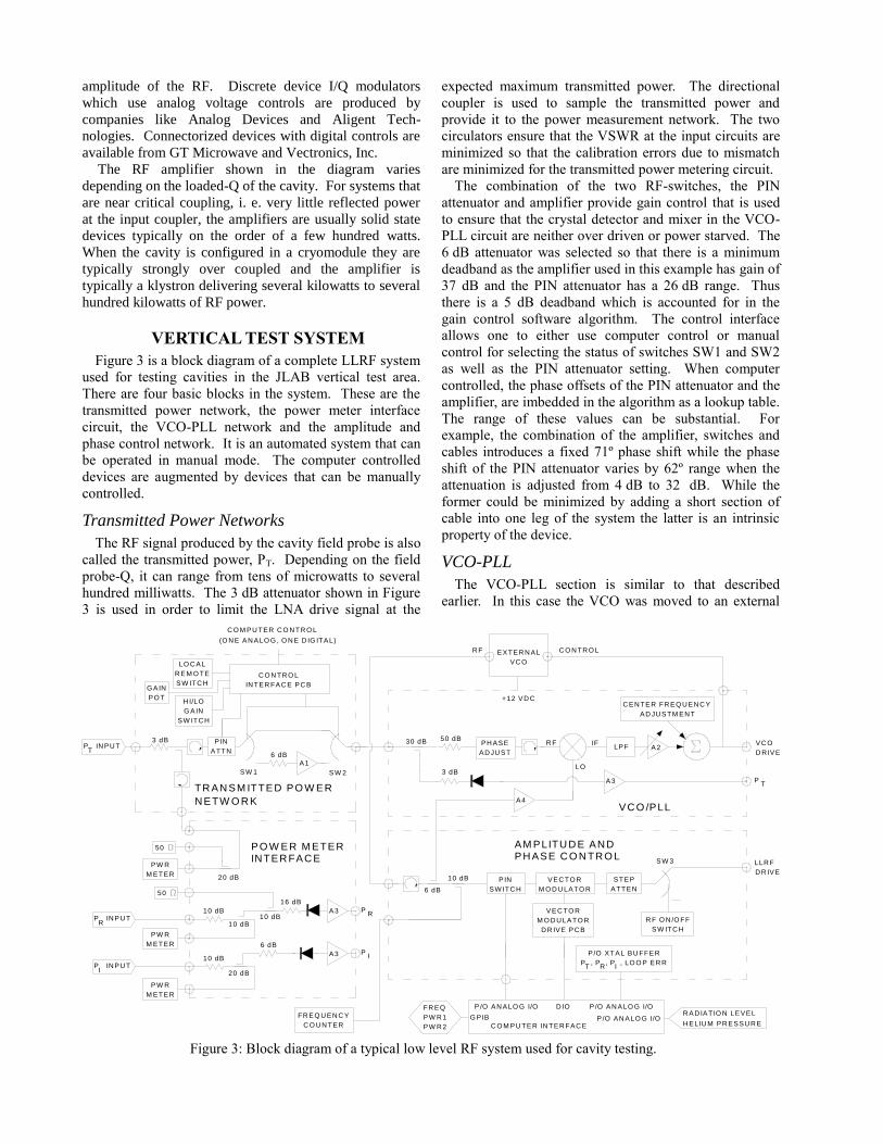
Figure 3 is a block diagram of a complete LLRF system
used for testing cavities in the JLAB vertical test area.
There are four basic blocks in the system. These are the
transmitted power network, the power meter interface
circuit, the VCO-PLL network and the amplitude and
phase control network. It is an automated system that can
be operated in manual mode. The computer controlled
devices are augmented by devices that can be manually
controlled.
Transmitted Power Networks
The RF signal produced by the cavity field probe is also
called the transmitted power, PT. Depending on the field
probe-Q, it can range from tens of microwatts to several
hundred milliwatts. The 3 dB attenuator shown in Figure
3 is used in order to limit the LNA drive signal at the
expected maximum transmitted power. The directional
coupler is used to sample the transmitted power and
provide it to the power measurement network. The two
circulators ensure that the VSWR at the input circuits are
minimized so that the calibration errors due to mismatch
are minimized for the transmitted power metering circuit.
The combination of the two RF-switches, the PIN
attenuator and amplifier provide gain control that is used
to ensure that the crystal detector and mixer in the VCO-
PLL circuit are neither over driven or power starved. The
6 dB attenuator was selected so that there is a minimum
deadband as the amplifier used in this example has gain of
37 dB and the PIN attenuator has a 26 dB range. Thus
there is a 5 dB deadband which is accounted for in the
gain control software algorithm. The control interface
allows one to either use computer control or manual
control for selecting the status of switches SW1 and SW2
as well as the PIN attenuator setting. When computer
controlled, the phase offsets of the PIN attenuator and the
amplifier, are imbedded in the algorithm as a lookup table.
The range of these values can be substantial. For
example, the combination of the amplifier, switches and
cables introduces a fixed 71º phase shift while the phase
shift of the PIN attenuator varies by 62º range when the
attenuation is adjusted from 4 dB to 32 dB. While the
former could be minimized by adding a short section of
cable into one leg of the system the latter is an intrinsic
property of the device.
VCO-PLL
The VCO-PLL section is similar to that described
earlier. In this case the VCO was moved to an external
AD JU STM EN T
C EN TER FR EQ U EN C Y
LPF
VC O /PLL
SW ITC H
G AIN
H I/LO
SW ITC H
R EM O TE
LO C AL
PO T
G AIN
VC O
+12 VD C
EXTER N AL
IF
LO
R F
AD JU ST
PH ASE
ATTEN
STEP
SW ITC H
PIN
M O D U LATO R
VEC TO R
VEC TO R
R F O N /O FF
SW ITC H
IT R
D R IVE PC B
R AD IATIO N LEVEL
H ELIU M PR ESSU R E
P , P , P , LO O P ER R
P/O XTAL BU FFER
M O D U LATO R
C O M PU TER C O N TR O L
(O N E AN ALO G , O N E D IG ITAL)
IN TER FAC E PC B
C O N TR O L
50 dB30 dB
10 dB
6 dB
6 dB
50
20 dB
16 dB
PIN3 dB
TP IN PU T
50
M ETER
PW R
10 dB
TR AN SM ITTED PO W ER
ATTN
D IO
C O M PU TER IN TER FAC E
6 dB
10 dB
20 dB
FR EQ U EN C Y
C O U N TERG PIB
PW R 2
PW R 1
FR EQ P/O AN ALO G I/O
PW R
M ETER
PW R
M ETER
R
P IN PU TI
PO W ER M ETER
10 dB
P IN PU T 10 dB
P/O AN ALO G I/O
P/O AN ALO G I/O
LLR F
D R IVE
VC O
D R IVE
PT
RP
IP
A1
A2
A3
A3
A3
SW 1 SW 2
SW 3
3 dB
N ETW O R K
IN TER FAC E
AM PLITU D E AN DPH ASE C O N TR O L
C O N TR O LR F
A4
Figure 3: Block diagram of a typical low level RF system used for cavity testing.
location so that it could be thermally stabilized.
Additionally, having it external allows one to use an
alternate VCO for different applications. The 3 dB and
50 dB attenuators are carefully selected as part of the
system optimization. The 50 dB attenuator is a major
contributor to setting the loop gain. In this case the VCO
is a broad band device with a sensitivity of about
5.6 MHz/V, thus the high value of attenuation. As a rule
of thumb, the attenuator should be chosen to be 10 dB
greater than the value at which the phase loop just starts to
oscillate, but still low enough that the loop will lock and
have a moderate lock range.
The 3 dB attenuator and the 30 dB coupler were chosen
such that the crystal detector is not power starved and is
still in the square law range when the loop is locked and
not oscillating. While the incident and reflected power
crystal detectors may be operated beyond the square law
range without compromising the measurements, one must
be careful to ensure that the transmitted power crystal
detector is operated in the square law range, (i.e. between
10 and 25 mV at the output, depending on the detector
and load combination) when making a decay measure-
ment. As a matter of convenience and in order to ensure
that there is adequate voltage available at the inputs to the
data acquisition card in the computer, the gain of the A3-
amplifiers was set to 400. Front panel connections
provide an easy means to observe these signals using an
oscilloscope. The A4 amplifier may be necessary
depending on the output level of the VCO and the input
requirements of the LO port on the mixer. In most
instances it is not necessary.
Amplitude and Phase Control
The output of the VCO is routed to the amplitude and
phase control section. The first device in that section is a
circulator. It is there to ensure that frequency pulling due
to impedance mismatches is minimized. Directional
couplers are placed in the circuit to couple power out for
the mixer local oscillator and the frequency counter. In
this way both devices always have a constant level signal
independent of the state of the output switches or
amplitude control circuits. The PIN switch provides a
means to pulse the RF on and off using either a pulse
generator or the computer controls. In addition to tuning
overcoupled cavities and verifying if the cavity is over
coupled or under coupled, this switch is used when
making decay measurements. The PIN switch is followed
by an I/Q modulator and a step attenuator that were
described previously. In most instances, computer control
is used and the step attenuator is not operated. The on-off
switch is actually an RF-relay that provides an easy way
for the operator to control the application of RF power. It
also provides a means to manually pulse the system. This
manual pulsed operation is frequently used in critically
coupled test of SRF cavities where cavity time constants
in excess of a few tenths of a second are not uncommon.
Power Meter Interface
The two critical considerations for the power meter
interface are stability of the components and low VSWR
in the power meter signal path. Neglecting either of these
will lead to unnecessary errors in the measurements. In
addition to the function of protecting the power heads
from damage due to peak RF power levels, the attenuators
act as matching devices which absorb any reflections due
to VSWR missmatch before they have a chance to
multiply. The crystal detectors are provided so that the
signals can be observed with an oscilloscope. Typically
the three traces that are observed are the transmitted
power signal, the reflected power signal and the VCO
drive signal. The auxiliary RF ports on the transmitted
and reflected power signals are provided so that a
spectrum analyzer may be used rather than the crystal
detectors.
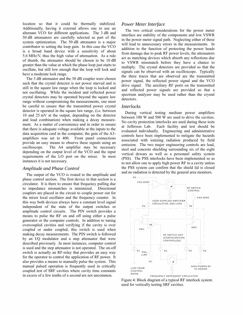
Interlocks
During vertical testing medium power amplifiers
between 100 W and 500 W are used to drive the cavities.
No cavity protection interlocks are used during these tests
at Jefferson Lab. Each facility and test should be
evaluated individually. Engineering and administrative
controls have been implemented to mitigate the hazards
associated with ionizing radiation produced by field
emission. The two major engineering controls are lead,
steel and concrete shielding surrounding six of the eight
vertical dewars as well as a personnel safety system
(PSS). The PSS interlocks have been implemented so as
to not allow one to apply high power RF to a cavity unless
the PSS system can confirm that the shield lid is closed
and no radiation is detected by the general area monitors.
LLR F
PSS
AC
P6P5
P4P3P2P1
PSS H PR F
AC
C O N TR O LLED )
(C O N FIG U R ATIO N
R F SW ITC H U N IT
1W
SW 2SW 1
C IR C U LATO R , AN D LO AD
U SER SU PPLIED AM PLIFIER
FR EQ U EN C Y D EPEN D EN T C IR C U LATO RR O O M
C O N TR O L
LLR F FR O M
PSS H PR F
C O N TR O L
R F SW ITC H
TO D EW AR
H IG H PO W ER R F
Figure 4: Block diagram of a typical RF interlock system
used for vertically testing SRF cavities.
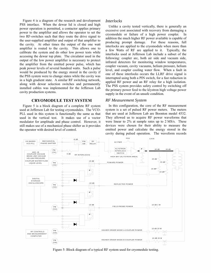
Figure 4 is a diagram of the research and development
PSS interface. When the dewar lid is closed and high
power operation is permitted, a contactor applies primary
power to the amplifier and allows the operator to set the
two RF-switches such that they route the drive signal to
the user-supplied amplifier and output of that amplifier to
the cavity. At other times the output of the one watt
amplifier is routed to the cavity. This allows one to
calibrate the system and do other low power tests while
accessing the dewar top plate. The circulator used in the
output of the low power amplifier is necessary to protect
the amplifier from the emitted power pulse, which has
peak power levels of several hundred watts. Such a pulse
would be produced by the energy stored in the cavity if
the PSS system were to change states while the cavity was
in a high gradient state. A similar RF switching network,
along with dewar selection switches and permanently
installed cables was implemented for the Jefferson Lab
cavity production systems.
CRYOMODULE TEST SYSTEM
Figure 5 is a block diagram of a complete RF system
used at Jefferson Lab for testing cryomodules. The VCO-
PLL used in this system is functionally the same as that
used in the vertical test. It makes use of a vector
modulator for amplitude and phase control. However, it
still makes use of a mechanical phase shifter as it provides
the operator with desired level of control.
Interlocks
Unlike a cavity tested vertically, there is generally an
excessive cost associated with recovery from damaging a
cryomodule or failure of a high power coupler. In
addition the much higher RF power available is capable of
producing prompt damage. For these reasons, full
interlocks are applied to the cryomodule when more than
a few Watts of RF are applied to it. Typically, the
interlocks used at Jefferson Lab include a subset of the
following: coupler arc, both air side and vacuum side,
infrared detectors for monitoring window temperatures,
coupler vacuum, cavity vacuums, helium pressure, helium
level, and coupler cooling water flow. When a fault in
one of these interlocks occurs the LLRF drive signal is
interrupted using both a PIN switch, for a fast reduction in
applied RF power and an RF relay for a high isolation.
The PSS system provides safety control by switching off
the primary power feed to the klystron high voltage power
supply in the event of an unsafe condition.
RF Measurement System
In this configuration, the core of the RF measurement
system is a set of pulsed RF power meters. The meters
that are used at Jefferson Lab are Boonton model 4532.
They allowed us to acquire RF power waveforms that
were linear to 2% at sample rates up to 2 MS/s. These
devices were chosen for their ability to measure the
emitted power and calculate the energy stored in the
cavity during pulsed operation. The waveform records
O SC ILLO SC O PE
STO R AG E
D IG ITAL
C O M PU TER
AN D M EASU R EM EN T
R F C O N TR O LS
40 dB
10 dB 1 W
PSS
AC PW R
H IG H ER O R D ER M O D E B-C O U PLER PO W ER
H IG H ER O R D ER M O D E A-C O U PLER PO W ER
C H 6
PM
C H 5
PM
10 dB 20 W
10 dB 20 W
H IG H BAY (KLYSTR O N AR EA)
C AVE
R EFLEC TED PO W ER
FO W AR D PO W ER
PM
C H 4
C H 3
PM
PM
C H 2
SW ITC H
IN TER LO C K
KLYSTR O N
10 dB*
20 dB
40 dB
10 dB*
20 dB
-10 dB
-10 dB
R ELAY
R F
SW
PIN
-10 dB
-6 dB
FIELD PR O BE PO W ER
VXI BASED
VC O -PLL PH ASE SH IFTER
M EC H AN IC AL
AR C , IRC O U PLER VAC U U M
BEAM LIN E VAC U U M
H ELIU M PR ESSU R E
C O U PLER W ATER FLO W
LIQ U ID LEVEL
PM
C H 16 dB
R F IN TER LO C KS
Figure 5: Block diagram of a typical RF system used for cryomodule testing.
were transferred from the instruments and processed on a
desktop computer in order to determine the cavity
parameters.
The four way splitters were added to the system so that
the RF signals could be used by other systems in parallel
with the standard acquisition process. The crystal
detectors were used for operator feedback. They were not
calibrated and were frequently operated beyond the square
law range. As in the VTA systems circulators and
attenuators were distributed throughout the system in
order to reduce the VSWR induced errors and to ensure
that the power meter readings were not affected by
changes in the configuration of the output ports on the 4-
way splitters. Polyphaser B50 or MR50 series lightning
arrestors were added to the HOM ports after several RF
power heads and medium power attenuators, rated at
20 W(CW) and 500 W(peak), were destroyed during SNS
cryomodule testing. Although precise measurements were
not captured, excessive power was observed on a crystal
detector when a cavity had a thermal quench. The leading
hypothesis is that the frequency shift associated with a
quench was more than several bandwidths of the HOM
couplers notch reject filter. Thus power levels on the
order of several tens of kilowatts was coupled out of the
cavity for a few hundred microseconds.
At times during the SNS testing a 20 kW CW klystron
was substituted for the 1 MW pulsed klystron. Iris plates
and stub tuners were placed in the waveguide circuit just
up stream of the fundamental power coupler, in order to
increase the external-Q of the system. Administrative
limits were put in place on the average cavity gradient
when operating in this mode. The limit was set such that
the equivalent average power rating of the coupler was
not exceeded.
CONSTRUCTION TECHNIQUES AND
AUTOMATION
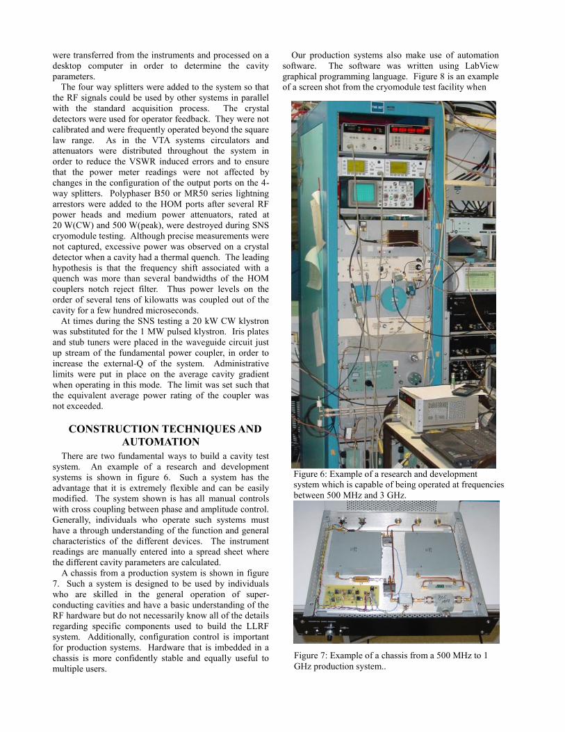
There are two fundamental ways to build a cavity test
system. An example of a research and development
systems is shown in figure 6. Such a system has the
advantage that it is extremely flexible and can be easily
modified. The system shown is has all manual controls
with cross coupling between phase and amplitude control.
Generally, individuals who operate such systems must
have a through understanding of the function and general
characteristics of the different devices. The instrument
readings are manually entered into a spread sheet where
the different cavity parameters are calculated.
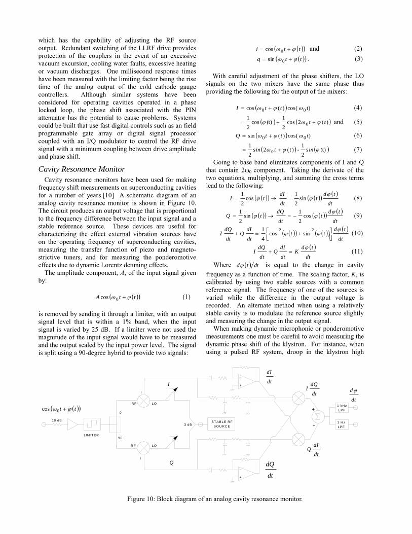
A chassis from a production system is shown in figure
7. Such a system is designed to be used by individuals
who are skilled in the general operation of super-
conducting cavities and have a basic understanding of the
RF hardware but do not necessarily know all of the details
regarding specific components used to build the LLRF
system. Additionally, configuration control is important
for production systems. Hardware that is imbedded in a
chassis is more confidently stable and equally useful to
multiple users.
Our production systems also make use of automation
software. The software was written using LabView
graphical programming language. Figure 8 is an example
of a screen shot from the cryomodule test facility when
Figure 6: Example of a research and development
system which is capable of being operated at frequencies
between 500 MHz and 3 GHz.
Figure 7: Example of a chassis from a 500 MHz to 1
GHz production system..

Figure 8: Image of a screen of the cryomodule production
software.
testing an SNS medium beta cavity. RF amplitude and
phase are controlled by entering a value for attenuation
and adjusting a phase knob. These values are combined
and transformed into a pair of control voltages for a
discrete I/Q modulator which is imbedded in a VXI-
packaged VCO-PLL. Cable calibration values are entered
into the program and the power meter readings are
corrected in the software. The waveforms in the upper
plot are of the reflected and forward power in Watts.
When operated in a pulsed mode each set of acquired
waveforms are processed to provide values for the
relevant parameters such as peak power levels, average
power levels, the stored energy at the end of the pulse, the
external-Q of all of the cavity ports, etc. Once a careful
measurement of the field probe external-Q is performed,
the value is entered into the screen and the lower trace
produces a time domain plot of the cavity gradient. Thus,
the operator has constant feedback as to the operating
point of the system. The software also has an interactive
routine for making calorimetric Q0 measurements. This
software controls the heaters as well as the state (on-off)
of the RF power. The routine also measures the rate of
rise of the helium pressure and calculates the power
dissipated by the cavity.
The vertical test software was written in a similar
manner. One of the more useful features of this software
is the interactive calibration routine with imbedded
operator instructions. Again the software has controls for
RF drive attenuation and phase controls which are
transformed to I and Q values. It is capable of doing
decay measurements in order to calculate the field probe
external-Q. Once the field probe-Q has been established,
a value is entered into the software and the operator has
continuous feedback of the incident power, 0Q , cavity
gradient, and field emission radiation levels. In both
software packages the error in percent for the relevant
variables is calculated and recorded to the data file as part
of the process and displayed on the screens.
AUXILIARY EQUIPMENT
In addition to standard RF test equipment such as
spectrum analyzers, network analyzers, low noise
amplifiers, etc. we have found it useful when making
microphonic measurements to have a dynamic signal
analyzer, and a cavity resonance monitor. Another
custom-made device that we used during production and
testing of SNS couplers, is know as a vacuum
conditioning controller. A similar device was used at
CERN for conditioning the LEP power couplers [8]
Coupler Conditioning Controller
A simple diagram of a vacuum conditioning controller
is shown in figure 9. As show, the system is capable of
processing two couplers connected in series. Typically
this connection is done through a rectangular waveguide
structure. The waveguide on the output coupler can be
either a fixed load or a sliding short [9]. The system uses
the analog vacuum signals from the gauge controllers to
control the klystron drive signal.
The difference between the set point and the actual each
of the actual vacuum signals is multiplied by 2.5. These
signals are diode added so that the larger of the two error
signals is passed and eventually controls the RF power
level. There is a gain adjustment and it as well as the set
point, the raw vacuum signal, and the PIN-attenuator
control voltage are monitored by a computer system
Figure 9: Block diagram of a vacuum conditioning system.
KLYSTR O N
IN TER LO C KS
AR C , C O O LIN G W ATER , ETC
VAC U U M
G AU G E
C O N TR O LLER
C O N TR O LLER
G AU G E
VAC U U M
TEST
C ELLC ELL
TEST
R EAD BAC K
C IR C U ITS
PR O TEC TIO N
KLYSTR O N
R F SO U R C E
PIN ATTN
R F
PIN SW ITC H
C O N TR O L-2 .5
+
++1
C O N TR O L
VAC U U M
-5V
-2.5
+
+
G AIN
VAC U U M
R EAD BAC K
SETPO IN T
-V
VAC U U M
LIN EAR IZATIO N
C IR C U IT
+
which has the capability of adjusting the RF source
output. Redundant switching of the LLRF drive provides
protection of the couplers in the event of an excessive
vacuum excursion, cooling water faults, excessive heating
or vacuum discharges. One millisecond response times
have been measured with the limiting factor being the rise
time of the analog output of the cold cathode gauge
controllers. Although similar systems have been
considered for operating cavities operated in a phase
locked loop, the phase shift associated with the PIN
attenuator has the potential to cause problems. Systems
could be built that use fast digital controls such as an field
programmable gate array or digital signal processor
coupled with an I/Q modulator to control the RF drive
signal with a minimum coupling between drive amplitude
and phase shift.
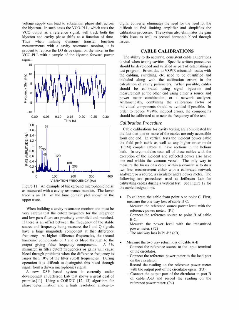
Cavity Resonance Monitor
Cavity resonance monitors have been used for making
frequency shift measurements on superconducting cavities
for a number of years.[10] A schematic diagram of an
analog cavity resonance monitor is shown in Figure 10.
The circuit produces an output voltage that is proportional
to the frequency difference between the input signal and a
stable reference source. These devices are useful for
characterizing the effect external vibration sources have
on the operating frequency of superconducting cavities,
measuring the transfer function of piezo and magneto-
strictive tuners, and for measuring the ponderomotive
effects due to dynamic Lorentz detuning effects.
The amplitude component, A, of the input signal given
by:
ttA 0cos (1)
is removed by sending it through a limiter, with an output
signal level that is within a 1% band, when the input
signal is varied by 25 dB. If a limiter were not used the
magnitude of the input signal would have to be measured
and the output scaled by the input power level. The signal
is split using a 90-degree hybrid to provide two signals:
tti 0cos and (2)
ttq 0sin . (3)
With careful adjustment of the phase shifters, the LO
signals on the two mixers have the same phase thus
providing the following for the output of the mixers:
t)cos()(cos 00 ttI (4)
)(2cos2
1(t)cos
2
1 0 tt and (5)
t)cos()(sin 00 ttQ (6)
(t)s2
1-)(2s
2
1 0 inttin (7)
Going to base band eliminates components of I and Q
that contain 2ω0 component. Taking the derivate of the
two equations, multiplying, and summing the cross terms
lead to the following:
dt
tdt
dt
dItI
sin
2
1cos
2
1 (8)
dt
tdt
dt
dQtQ
cos
2
1sin
2
1 (9)
dt
tdtt
dt
dIQ
dt
dQI
22
sincos4
1 (10)
dt
tdK
dt
dIQ
dt
dQI
(11)
Where dttd is equal to the change in cavity
frequency as a function of time. The scaling factor, K, is
calibrated by using two stable sources with a common
reference signal. The frequency of one of the sources is
varied while the difference in the output voltage is
recorded. An alternate method when using a relatively
stable cavity is to modulate the reference source slightly
and measuring the change in the output signal.
When making dynamic microphonic or ponderomotive
measurements one must be careful to avoid measuring the
dynamic phase shift of the klystron. For instance, when
using a pulsed RF system, droop in the klystron high
LPF
1 H z
LPF
1 kH z
+
+
_
+
_
+
SO U R C E
STABLE R F3 dB
I
I
LO
LOR F
R F
90
0
LIM ITER
10 dB
tt 0cos
dt
dQI
Q
I
dt
dQ
dt
dI
dt
dIQ
dt
d
Figure 10: Block diagram of an analog cavity resonance monitor.
voltage supply can lead to substantial phase shift across
the klystron. In such cases the VCO-PLL, which uses the
VCO output as a reference signal, will track both the
klystron and cavity phase shifts as a function of time.
Thus when making dynamic transfer function
measurements with a cavity resonance monitor, it is
prudent to replace the LO drive signal on the mixer in the
VCO-PLL with a sample of the klystron forward power
signal.
-10
-5
0
5
10
15
0.00 0.05 0.10 0.15 0.20 0.25 0.30
Time (s)
Fre
quency S
hift
(Hz)
0
0.2
0.4
0.6
0.8
1
1.2
1.4
1.6
1.8
0 100 200 300 400
VIBRATION FREQUENCY (Hz)
RM
S A
MP
LIT
UD
E (
Hz)
208180
120
58
3035
46
Figure 11: An example of background microphonic noise
as measured with a cavity resonance monitor. The lower
trace is an FFT of the time domain plot shown in the
upper trace.
When building a cavity resonance monitor one must be
very careful that the cutoff frequency for the integrator
and low pass filters are precisely controlled and matched.
If there is an offset between the frequency of the stable
source and frequency being measure, the I and Q signals
have a large magnitude component at that difference
frequency. At higher difference frequencies, the second
harmonic components of I and Q bleed through to the
output giving false frequency components. A 5%
mismatch in filter cutoff frequencies or gains will cause
bleed through problems when the difference frequency is
larger than 10% of the filter cutoff frequencies. During
operation it is difficult to distinguish this bleed through
signal from a driven microphonics signal.
A new DSP based system is currently under
development at Jefferson Lab that shows a great deal of
promise.[11] Using a CORDIC [12, 13] algorithm for
phase determination and a high resolution analog-to-
digital converter eliminates the need for the need for the
difficult to find limiting amplifier and simplifies the
calibration processes. The system also eliminates the gain
drifts issue as well as second harmonic bleed through
issues.
CABLE CALIBRATIONS
The ability to do accurate, consistent cable calibrations
is vital when testing cavities. Specific written procedures
should be developed and verified as part of establishing a
test program. Errors due to VSWR mismatch issues with
the cabling, switching, etc. need to be quantified and
included along with the calibration errors in the
calculation of cavity parameters. When possible, cables
should be calibrated using signal injection and
measurement at the other end using either a source and
power meter combination, or a network analyzer.
Arithmetically, combining the calibration factor of
individual components should be avoided if possible. In
order to reduce VSWR induced errors, the components
should be calibrated at or near the frequency of the test.
Calibration Procedure
Cable calibrations for cavity testing are complicated by
the fact that one or more of the cables are only accessible
from one end. In vertical tests the incident power cable
the field prob cable as well as any higher order mode
(HOM) coupler cables all have sections in the helium
bath. In cryomodules tests all of these cables with the
exception of the incident and reflected power also have
one end within the vacuum vessel. The only way to
measure the losses of a cable within a cryostat is to do a
two loss measurement either with a calibrated network
analyzer; or a source, a circulator and a power meter. The
following are procedures used at Jefferson Lab for
calibrating cables during a vertical test. See Figure 12 for
the cable designations.
To calibrate the cable from point A to point C. First,
measure the one way loss of cable B-C.
- Measure the reference source power level with the
reference power meter. (P1)
- Connect the reference source to point B of cable
B-C.
- Measure the power level with the transmitted
power meter. (P2)
- The one way loss is P1-P2 (dB)
Measure the two way return loss of cable A-B
- Connect the reference source to the input terminal
of the circulator.
- Connect the reference power meter to the load port
on the circulator.
- Record the reading on the reference power meter
with the output port of the circulator open. (P3)
- Connect the output port of the circulator to port B
of cable A-B and record the reading on the
reference power meter. (P4)

- The two way return loss of cable A-B is:
.43 PP
The cable calibration for the transmitted power meter,
A-C path, is:
(dB) 2
4321 PPPPC AC
(12)
To calibrate the cable from point D to F and D to G
Measure the forward power calibration from E to F
- Connect the reference power meter to point E of
the cable from the RF drive source.
- Turn on the RF drive source and increase the power
until the power level on the reference power meter
is about 2/3 of the maximum allowed.
- Record the power levels on the reference meter
(P5) and the incident meter (P6)
Measure the reflected power calibration from E to G
- Turn off the RF source drive
- Measure the reference source power level with the
reference power meter. (P7)
- Connect the reference source to point E of the path
E-G.
- Measure the power level with the reflected power
meter. (P8)
Measure the two way loss for the cable D-E with a
slightly detuned cavity.
- Connect the RF drive source to the cavity at
point E.
- Turn on the RF drive source and apply power to
the cavity at a frequency about 10 to 20 kHz
higher or lower than the cavity’s resonant
frequency.
- Measure the incident (P9) and reflected power
(P10) with the respective meters.
The cable calibration for the incident, F-D path, and
reflected power, G-D path, meters are:
(dB) 2
1098765 PPPPPPC INC
(13)
(dB) 2
1098*37*356 PPPPPPC REFL
(14)
Calibration Verification
Two ways to verify calibration procedures are to
calibrate the system using an external cable in place of the
cable within the dewar then do one or both of the
following. For the field probe cable calibration and
reflected power calibration inject a known signal level into
the external cable and measure the power using the
calibrated power meter. For the forward power
calibration connect the external cable to a remote power
meter; inject a signal into the drive cable using the RF
drive source; and measure the power using the remote
power meter and the incident power meter. In both cases
it can be a good exercise to vary the frequency over an 1
MHz to 2 MHz range and compare the values over the
range. Variations of more than a few percent the readings
from the calibrated power meter and the reference power
meter indicates excessive VSWR mismatches somewhere
in the system.
A third way to verify the calibration and to look for
VSWR problems in the incident power cable is to use the
RF drive source to apply power to either an open test
cable that has been calibrated or a detuned cavity. Record
the values of the calibrated forward and reflected power
as a function of frequency. They should be equal at all
times. A variation in the difference between the two
calibrated power measurements indicates a VSWR
problem in the system. Figure 13 shows the results of
such a measurement. The cabling with the minimal errors
as a function of frequency made use of attenuators
distributed throughout the signal path.
-8.0%
-6.0%
-4.0%
-2.0%
0.0%
2.0%
4.0%
804.0 804.5 805.0 805.5 806.0
FREQUENCY (MHz)
DIF
FE
RE
NC
E F
RO
M 8
05
MH
z
Figure 13: Difference between RF power measurements
calibrated at 805 MHz and those taken at nearby
frequencies for several different signal paths.
CABLE BREAKDOWN
When performing vertical tests at 2 K the incident
power cables must pass through the low pressure helium
gas in order to get to the fundamental power coupler.
C IR C U LATO R
R EFER EN C E
TYPIC AL
30 dB
G
F
E
D
C
B
A
SO U R C E
R F D R IVE
SO U R C E
R EFER EN C E
M ETER
PO W ER
R EFER EN C E
M ETER
PO W ER
TR AN SM ITTED
M ETER
PO W ER
IN C ID EN T
M ETER
PO W ER
R EFLEC TED
Figure 12: Diagram of the cabling and power meters
used for a typical vertical test
The pressure at which helium goes superfluid is 35 Torr,
and systems are typically operated at pressures between
20 and 25 Torr. Operating in this pressure regime with the
typical dimensions of medium power RF connectors (i.e.
1 mm to 5 mm) means that the connectors are operating at
or near the Pasching minimum of 4 Torr-cm. At this
pressure-distance product the breakdown voltage in
helium gas is minimized [14], and thus, there is a
reasonable probability that glow discharges will occur.
Work done by MacDonald and Brown in 1949 indicated
that the minimum pressure for RF breakdown in helium
was between 8 and 30 Torr depending on the
geometery.[15] The probability of breakdown is further
enhanced by field emission radiation. In general, this
phenomenon is not new and has been extensively studied
by individuals working in the satellite industry where it is
known as multipactor breakdown. [16]
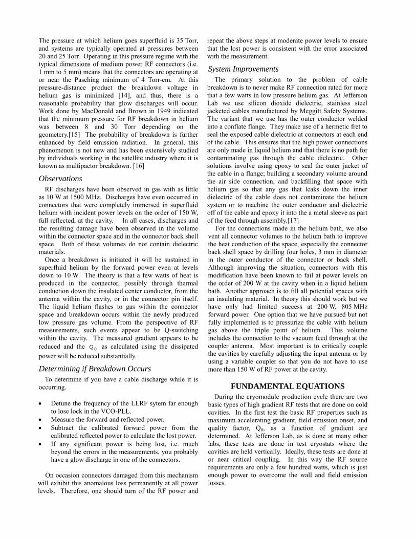
Observations
RF discharges have been observed in gas with as little
as 10 W at 1500 MHz. Discharges have even occurred in
connectors that were completely immersed in superfluid
helium with incident power levels on the order of 150 W,
full reflected, at the cavity. In all cases, discharges and
the resulting damage have been observed in the volume
within the connector space and in the connector back shell
space. Both of these volumes do not contain dielectric
materials.
Once a breakdown is initiated it will be sustained in
superfluid helium by the forward power even at levels
down to 10 W. The theory is that a few watts of heat is
produced in the connector, possibly through thermal
conduction down the insulated center conductor, from the
antenna within the cavity, or in the connector pin itself.
The liquid helium flashes to gas within the connector
space and breakdown occurs within the newly produced
low pressure gas volume. From the perspective of RF
measurements, such events appear to be Q-switching
within the cavity. The measured gradient appears to be
reduced and the 0Q as calculated using the dissipated
power will be reduced substantially.
Determining if Breakdown Occurs
To determine if you have a cable discharge while it is
occurring.
Detune the frequency of the LLRF sytem far enough
to lose lock in the VCO-PLL.
Measure the forward and reflected power.
Subtract the calibrated forward power from the
calibrated reflected power to calculate the lost power.
If any significant power is being lost, i.e. much
beyond the errors in the measurements, you probably
have a glow discharge in one of the connectors.
On occasion connectors damaged from this mechanism
will exhibit this anomalous loss permanently at all power
levels. Therefore, one should turn of the RF power and
repeat the above steps at moderate power levels to ensure
that the lost power is consistent with the error associated
with the measurement.
System Improvements
The primary solution to the problem of cable
breakdown is to never make RF connection rated for more
that a few watts in low pressure helium gas. At Jefferson
Lab we use silicon dioxide dielectric, stainless steel
jacketed cables manufactured by Meggitt Safety Systems.
The variant that we use has the outer conductor welded
into a conflate flange. They make use of a hermetic fret to
seal the exposed cable dielectric at connectors at each end
of the cable. This ensures that the high power connections
are only made in liquid helium and that there is no path for
contaminating gas through the cable dielectric. Other
solutions involve using epoxy to seal the outer jacket of
the cable in a flange; building a secondary volume around
the air side connection; and backfilling that space with
helium gas so that any gas that leaks down the inner
dielectric of the cable does not contaminate the helium
system or to machine the outer conductor and dielectric
off of the cable and epoxy it into the a metal sleeve as part
of the feed through assembly.[17]
For the connections made in the helium bath, we also
vent all connector volumes to the helium bath to improve
the heat conduction of the space, especially the connector
back shell space by drilling four holes, 3 mm in diameter
in the outer conductor of the connector or back shell.
Although improving the situation, connectors with this
modification have been known to fail at power levels on
the order of 200 W at the cavity when in a liquid helium
bath. Another approach is to fill all potential spaces with
an insulating material. In theory this should work but we
have only had limited success at 200 W, 805 MHz
forward power. One option that we have pursued but not
fully implemented is to pressurize the cable with helium
gas above the triple point of helium. This volume
includes the connection to the vacuum feed through at the
coupler antenna. Most important is to critically couple
the cavities by carefully adjusting the input antenna or by
using a variable coupler so that you do not have to use
more than 150 W of RF power at the cavity.
FUNDAMENTAL EQUATIONS
During the cryomodule production cycle there are two
basic types of high gradient RF tests that are done on cold
cavities. In the first test the basic RF properties such as
maximum accelerating gradient, field emission onset, and
quality factor, Q0, as a function of gradient are
determined. At Jefferson Lab, as is done at many other
labs, these tests are done in test cryostats where the
cavities are held vertically. Ideally, these tests are done at
or near critical coupling. In this way the RF source
requirements are only a few hundred watts, which is just
enough power to overcome the wall and field emission
losses.

In the second type of test the cavities are installed in the
final cryostat and they are typically strongly over coupled.
This presents a problem as the errors in lost RF power get
excessive when 95% to 99.9% of the incident power is
reflected back out of the fundamental power coupler.
Thus, during cryomodule tests the RF heat load is
measured calorimetrically.
Table 1: Common variables used when discussing
superconducting RF cavities.
Symbol Variable Name Units
Qr / Geometric Shunt Impedance Ω/m
G Geometry Factor Ω
E Electric Field V/m
L Electrical Length M
0 Cavity Frequency s-1
U Stored Energy J
sr Surface Resistance Ω
CT Critical Temperature K
XP RF Power at Port X W
emitP Emitted Power W
R Shunt Impedance Ω
T Operational Temperature K
residr Residual Surface Resistance Ω
0Q Intrinsic Quality Factor
FPCQ Fundamental Power Coupler
Coupling Factor
2 , QQ FP Field Probe Coupling Factor
CR Coupling Impedance Ω/m
I Beam Current A
MI Matching Current A
dispP Dissipated Power W
Decay Time s
r Shunt Impedance Per
Unit Length Ω/m
Summary of Variables Names and Units
Table 1 is a listing of the variables commonly used
when discussing superconducting cavities, their names
and associated units. The equations that follow were
extracted from several sources over the years [18, 19, 20].
They are the basis for many of the RF measurements and
associated calculations associated with SRF cavities. A
good general reference for this material is entitled RF
Superconductivity for Accelerators, by Padamsee,
Knobloch and Hayes.
The Appendix of this document contains a complete set
of equations used for making cavity measurements, near
critical coupling using the decay method and the CW
method as well as for making measurements of strongly
over coupled systems. Additionally, the appendix
contains equations used for calculating the errors
associated with the calculated values.
The critical variable for calculating the RF parameters
of a superconducting cavity is the shunt impedance, which
relates the stored energy to the effective accelerating
gradient, peak electric field, and peak magnetic field for
any given mode. It is determined using electromagnetic
simulation tools such as Mafia or Superfish. One should
be careful in applying this variable as there are different
definitions of shunt impedance, R, and geometric shunt
impedance, (r/Q), in use[21]. For this paper, both
variables are based on the definition that PVR2
,
which includes the transient time factor.
General RF Measurement Equations
The following are general RF equations that apply to
SRF cavities:
Qr
LEU
/0
2
(15)
Qr
L
Q
E
Q
UP
/
2
0
(16)
adingElectronLoQrSGQ ||/0 (17)
resid
TT
S reT
fGHzKr
c
/95.12
)2/(410 (18)
FPCFPFPCL QQQQQ ||||0 (19)
)/( QrQR LC (20)
CM REI / (22)
The power delivered to the beam is:
LEIPBeam (23)
The coupling factor, β, is a measure of the efficiency of
coupling RF power into the system it is given by:
incidentreflected
incidentreflected
PPC
PPC
/1
/1
(24)
where C is 1 for the under coupled and -1 for the over
coupled case. For a cavity which are perfectly tuned and
with the beam on crest, the power required by the klystron
is:
C
CKly
R
IRELP
2
4
1
(25)
2
)/(
1
4
1r/QIQE
Qr
L
QL
L
(26)

The Power reflected back to the circulator is:
C
CRef
R
IRELP
2
4
1
(27)
2)/(
1
4
1r/QIQE
Qr
L
QL
L
(28)
The time dependent complex differential equation
where K
is the incident wave amplitude in Watts , d
is the (time varying) detune angle, and Lf Q2/0 :
IRL
RK
dt
Ed
ωE
ω
ω-j C
C
ff
d
2
11 (29)
Adding microphonics and the effects of the difference
cavity center frequency 0f and that of the RF source, f ,
and the beam current, I, being off crest by B leads to the
equation (30) as the power required of the klystron.[20]
2
0
0
20
sin2
cos
4
1
BCL
BC
C
Kly
RIEf
fQ
RIE
R
LP
(30)
When testing strongly overcoupled cavities 1 ,
0QQ L and FPL QQ which means that
FPCL QQ , in this case.
2LQ (31)
L
QrQPE LIncident
)/(
)1(
42
(32)
Because 1 , 41
4
and, in this case.
L
QrQPE LIncident
)/(4 (33)
Although using the above forward power to calculate
gradient is a reasonable technique, practical experience
says that there can easily be as much as 25% difference
between the gradient as calculated using the forward
technique power and the emitted power technique or
using a well calibrated field probe. This difference can be
reduced by properly tuning the phase locked loop,
variable frequency system, or the cavity for a fixed
frequency system.
Error Analysis
Most of the error analysis done when making cavity
measurements can be done using a few fundamental
equations as follows:
22)(
B
B
A
A
AB
AB (34)
2
22)(
BA
BA
BA
BA
(35)
A
A
A
A
2
1)( (36)
A
A
AA
AA
2
)( (37)
The first two equations assume that the errors are
Gaussian and uncorrelated. The factors of ½ and 2 found
in equations (36) and (37) are because the errors are
correlated. There are occasions, for instance the emitted
power measurement, when using the simple equations is
not appropriate and can lead to non causal errors. In such
cases it is a simple matter to perform a Monte Carlo
calculation to determine the dependencies. Additionally,
care must be taken when chaining together calculations.
For instance, determination of FPQ for a strongly over
coupled cavity includes any fixed calibration error in the
transmitted power signal. If the calculated value of FPQ
is used to later calculate the gradient based on the
transmitted power signal (using the same cable calibration
factor), the error in the gradient should not include the
transmitted power cable calibration factor. In this case the
error in the transmitted power based gradient should only
contain the error in the linearity of the power meter
measurement and the error associated with FPQ .
CRITICALLY COUPLED CAVITY
MEASUREMENTS
When a cavity is near critical coupling, the process for
determining the cavity parameters of FPQQE and , , 0 is as
follows. The RF frequency and phase are controlled by a
VCO-PLL. The phase is carefully adjusted to minimize
the reflected power, which also maximizes the transmitted
(i.e., the field probe) power. Then a decay measurement
is made which determines the values of FPQQE and , , 0 .
Once the results of the decay measurement is completed,
FPQ is used along with the RF power measurements to
calculate 0 and QE .
The Decay Measurement
The decay measurement is initiated by pulsing RF
power on and off so that one can determine if the cavity is
over coupled or under coupled. Figure 14 shows the
shape of the reflected power pulse for the different
coupling conditions. Stable gradient is established and
the steady state forward, reflected and transmitted power
levels, ( TranRefFwd PPP and , , respectively) are recorded.
Next, the cavity drive signal is turned off and the decay
time constant, , of the resulting transmitted power
transient is determined using a crystal detector, a spectrum
analyzer or a pulsed RF power meter.
The decay time, , is used to calculate a value for the
loaded-Q, LQ . TranRefFwdL PPPQ and , ,, are used to
calculate 0Q . The gradient may then be calculated as:

L
QrQPE Loss
)/(0 (38)
and the field probe-Q can be calculated as:
Qr
LPEQ TranFP
/
2 (39)
As stated earlier, the operator must determine if the
cavity is over coupled or under coupled prior to
calculating the cavity parameters using the decay
measurement technique. Typically a crystal detector is
placed on the reflected power signal and the resultant
signal is observed on an oscilloscope. Figure 14 is a
depiction of the reflected power waveforms produced by a
properly tuned cavity under different, near critical
coupling, conditions.
In all of the reflected power pulses, the first peak has
the same magnitude as the reflected power signal when
the cavity is detuned. When the cavity is over coupled,
the emitted power pulse, i.e. the second peak, is larger
than the first peak. When the phase loop is properly tuned
the minimum after the first peak goes through zero.
When the cavity is critically coupled, the leading and
trailing peaks are of equal magnitude and the reflected
power goes to zero at the end of the pulse. When the
cavity is under coupled the secondary peak, if there is
one, is smaller than the first peak and the reflected power
signal does not go to zero during the pulse.
U N D ER C O U PLED < 1/3
U N D ER C O U PLED 1< < 1/3
O VER C O U PLED >1
C R ITIC ALLY C O U PLED =1
FIELD PR O BE PO W ERFO R W AR D PO W ER
Figure 14: Upper four traces are depictions of reflected
power waveforms for various coupling states. The lower
two traces are the corresponding forward and field probe
pulse shapes.
CW Measurements
Once a value has been determined for the field probe-Q
the calculations become much simpler. The gradient is
given by:
L
QrQPE FPTrans
)/( (40)
and the quality factor is given by:
Qr
LPEQ Loss
/
2
0 (41)
Decay Measurement Errors
Crystal detectors are frequently used to measure the
decay time, . Other alternatives included using a pulsed
RF power meter as discussed earlier or using a spectrum
analyzer set up to do a zero span, time domain
measurement. The crystal detector measurement relies on
the fact that the crystal detector is operating within the
square law range. In this power, or output voltage, range
the output voltage is proportional to the RF power.
Using the half power, decay time constant technique, a
properly terminated crystal detector can be used to make a
+/- 3% measurement of the cavity decay time constant if
the peak detector voltage is below 10 mV. If, for
example, the same crystal detector were inadvertently
used at 100 mV, the measured decay time would be
overestimated by about 40%, the calculated 0Q would be
40% higher than the actual value and the calculated cavity
gradient would be 18% higher than the actual value.
Another source of decay measurement errors is changes
in the loaded-Q during the decay measurement. Usually
this is due to non linear effects such as field emission
loading. As the energy stored in the cavity is emitted out
of the fundamental power port, the gradient in the cavity
is reduced; the field emission loading is reduced; and the
loaded-Q is increased. This also occurs if the cavity has a
strong Q-slope. The logarithmic slope of the decaying
power is . In general is a function of E, or
equalivently EQ 0 . In such cases the decay slope at the
start of the decay must be used, or a systematic error will
lead to calculated 0Q and E values that are larger than
the actual values.
Lost Power Measurement Errors
Because the lost power is a difference between three
power meter measurements, the error is given by the
following:
2
222
TranRefFwd
TranRefFwd
Loss
Loss
PPP
PPP
P
P
(42)
Thus the error in the lost power increases dramatically
when the reflected power approaches that of the forward
power. Remember, when the cavity is critically coupled
1 ; the reflected power is equal to zero and virtually
all of the forward power goes into wall heating. As 1
increases much above three or below one third the
reflected power starts to become a substantial fraction of
the wall heating power and the error in the lost power
increases. This is the major contributor to the error is CW
0Q measurements and decay measurement based of the
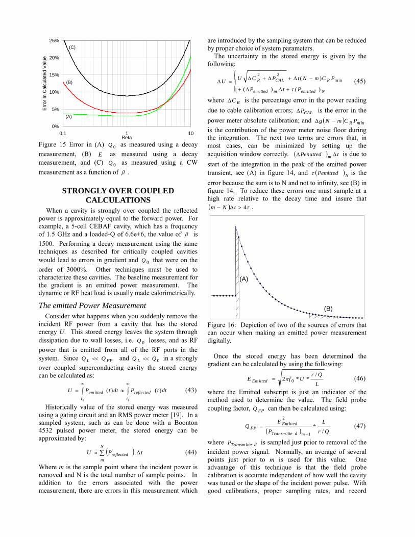
gradient. Figure 15 are plots of the error in gradient and
0Q as a function of . The calculations assume that the
power meter measurements, including cable calibrations
are %7 , the linearity of the power meters is %2 , that
is known to %3 and that the power meters are
operated well above their noise floor. Under these
conditions, the error in the decay based gradient
measurement and the CW 0Q measurement vary because
of the errors in the lost power calculation. Thus it is best
to try to make all of the measurements when 25.0 .
0%
5%
10%
15%
20%
25%
0.1 1 10Beta
Err
or
In C
alc
ula
ted
Va
lue
(A)
(B)
(C)
Figure 15 Error in (A) 0Q as measured using a decay
measurement, (B) E as measured using a decay
measurement, and (C) 0Q as measured using a CW
measurement as a function of .
STRONGLY OVER COUPLED
CALCULATIONS
When a cavity is strongly over coupled the reflected
power is approximately equal to the forward power. For
example, a 5-cell CEBAF cavity, which has a frequency
of 1.5 GHz and a loaded-Q of 6.6e+6, the value of is
1500. Performing a decay measurement using the same
techniques as described for critically coupled cavities
would lead to errors in gradient and 0Q that were on the
order of 3000%. Other techniques must be used to
characterize these cavities. The baseline measurement for
the gradient is an emitted power measurement. The
dynamic or RF heat load is usually made calorimetrically.
The emitted Power Measurement
Consider what happens when you suddenly remove the
incident RF power from a cavity that has the stored
energy U. This stored energy leaves the system through
dissipation due to wall losses, i.e. 0Q losses, and as RF
power that is emitted from all of the RF ports in the
system. Since FPL QQ and 0QQ L in a strongly
over coupled superconducting cavity the stored energy
can be calculated as:
dttPdttPU
t
reflected
t
emitted )()(
00
(43)
Historically value of the stored energy was measured
using a gating circuit and an RMS power meter [19]. In a
sampled system, such as can be done with a Boonton
4532 pulsed power meter, the stored energy can be
approximated by:
tPU
N
m
reflected (44)
Where m is the sample point where the incident power is
removed and N is the total number of sample points. In
addition to the errors associated with the power
measurement, there are errors in this measurement which
are introduced by the sampling system that can be reduced
by proper choice of system parameters.
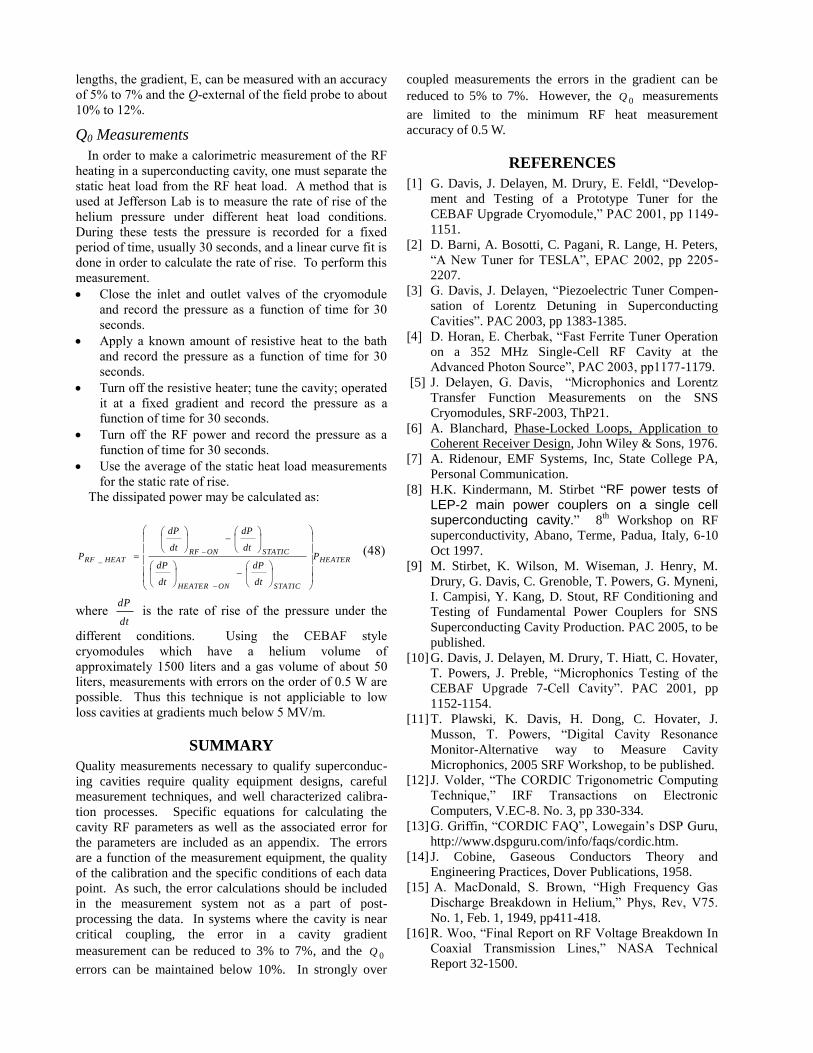
The uncertainty in the stored energy is given by the
following:
Nemittedmemitted
RCALR
PtP
PCmNtPCUU
)()(
)( min
22
(45)
where RC is the percentage error in the power reading
due to cable calibration errors; CALP is the error in the
power meter absolute calibration; and minR PCmNg
is the contribution of the power meter noise floor during
the integration. The next two terms are errors that, in
most cases, can be minimized by setting up the
acquisition window correctly. tPenuttedm is due to
start of the integration in the peak of the emitted power
transient, see (A) in figure 14, and N
Pemitted is the
error because the sum is to N and not to infinity, see (B) in
figure 14. To reduce these errors one must sample at a
high rate relative to the decay time and insure that
4 tNm .
(A)
(B)
Figure 16: Depiction of two of the sources of errors that
can occur when making an emitted power measurement
digitally.
Once the stored energy has been determined the
gradient can be calculated by using the following:
L
QrUfE Emitted
/**2 0 (46)
where the Emitted subscript is just an indicator of the
method used to determine the value. The field probe
coupling factor, FPQ can then be calculated using:
Qr
L
P
EQ
mdTransmitte
EmittedFP
/*
1
2
(47)
where dTransmitteP is sampled just prior to removal of the
incident power signal. Normally, an average of several
points just prior to m is used for this value. One
advantage of this technique is that the field probe
calibration is accurate independent of how well the cavity
was tuned or the shape of the incident power pulse. With
good calibrations, proper sampling rates, and record
lengths, the gradient, E, can be measured with an accuracy
of 5% to 7% and the Q-external of the field probe to about
10% to 12%.
Q0 Measurements
In order to make a calorimetric measurement of the RF
heating in a superconducting cavity, one must separate the
static heat load from the RF heat load. A method that is
used at Jefferson Lab is to measure the rate of rise of the
helium pressure under different heat load conditions.
During these tests the pressure is recorded for a fixed
period of time, usually 30 seconds, and a linear curve fit is
done in order to calculate the rate of rise. To perform this
measurement.
Close the inlet and outlet valves of the cryomodule
and record the pressure as a function of time for 30
seconds.
Apply a known amount of resistive heat to the bath
and record the pressure as a function of time for 30
seconds.
Turn off the resistive heater; tune the cavity; operated
it at a fixed gradient and record the pressure as a
function of time for 30 seconds.
Turn off the RF power and record the pressure as a
function of time for 30 seconds.
Use the average of the static heat load measurements
for the static rate of rise.
The dissipated power may be calculated as:
HEATER
STATICONHEATER
STATICONRFHEATRF P
dt
dP
dt
dP
dt
dP
dt
dP
P
_
(48)
where dt
dP is the rate of rise of the pressure under the
different conditions. Using the CEBAF style
cryomodules which have a helium volume of
approximately 1500 liters and a gas volume of about 50
liters, measurements with errors on the order of 0.5 W are
possible. Thus this technique is not appliciable to low
loss cavities at gradients much below 5 MV/m.
SUMMARY
Quality measurements necessary to qualify superconduc-
ing cavities require quality equipment designs, careful
measurement techniques, and well characterized calibra-
tion processes. Specific equations for calculating the
cavity RF parameters as well as the associated error for
the parameters are included as an appendix. The errors
are a function of the measurement equipment, the quality
of the calibration and the specific conditions of each data
point. As such, the error calculations should be included
in the measurement system not as a part of post-
processing the data. In systems where the cavity is near
critical coupling, the error in a cavity gradient
measurement can be reduced to 3% to 7%, and the 0Q
errors can be maintained below 10%. In strongly over
coupled measurements the errors in the gradient can be
reduced to 5% to 7%. However, the 0Q measurements
are limited to the minimum RF heat measurement
accuracy of 0.5 W.
REFERENCES
[1] G. Davis, J. Delayen, M. Drury, E. Feldl, “Develop-
ment and Testing of a Prototype Tuner for the
CEBAF Upgrade Cryomodule,” PAC 2001, pp 1149-
1151.
[2] D. Barni, A. Bosotti, C. Pagani, R. Lange, H. Peters,
“A New Tuner for TESLA”, EPAC 2002, pp 2205-
2207.
[3] G. Davis, J. Delayen, “Piezoelectric Tuner Compen-
sation of Lorentz Detuning in Superconducting
Cavities”. PAC 2003, pp 1383-1385.
[4] D. Horan, E. Cherbak, “Fast Ferrite Tuner Operation
on a 352 MHz Single-Cell RF Cavity at the
Advanced Photon Source”, PAC 2003, pp1177-1179.
[5] J. Delayen, G. Davis, “Microphonics and Lorentz
Transfer Function Measurements on the SNS
Cryomodules, SRF-2003, ThP21.
[6] A. Blanchard, Phase-Locked Loops, Application to
Coherent Receiver Design, John Wiley & Sons, 1976.
[7] A. Ridenour, EMF Systems, Inc, State College PA,
Personal Communication.
[8] H.K. Kindermann, M. Stirbet “RF power tests of LEP-2 main power couplers on a single cell superconducting cavity.” 8
th Workshop on RF
superconductivity, Abano, Terme, Padua, Italy, 6-10
Oct 1997.
[9] M. Stirbet, K. Wilson, M. Wiseman, J. Henry, M.
Drury, G. Davis, C. Grenoble, T. Powers, G. Myneni,
I. Campisi, Y. Kang, D. Stout, RF Conditioning and
Testing of Fundamental Power Couplers for SNS
Superconducting Cavity Production. PAC 2005, to be
published.
[10] G. Davis, J. Delayen, M. Drury, T. Hiatt, C. Hovater,
T. Powers, J. Preble, “Microphonics Testing of the
CEBAF Upgrade 7-Cell Cavity”. PAC 2001, pp
1152-1154.
[11] T. Plawski, K. Davis, H. Dong, C. Hovater, J.
Musson, T. Powers, “Digital Cavity Resonance
Monitor-Alternative way to Measure Cavity
Microphonics, 2005 SRF Workshop, to be published.
[12] J. Volder, “The CORDIC Trigonometric Computing
Technique,” IRF Transactions on Electronic
Computers, V.EC-8. No. 3, pp 330-334.
[13] G. Griffin, “CORDIC FAQ”, Lowegain’s DSP Guru,
http://www.dspguru.com/info/faqs/cordic.htm.
[14] J. Cobine, Gaseous Conductors Theory and
Engineering Practices, Dover Publications, 1958.
[15] A. MacDonald, S. Brown, “High Frequency Gas
Discharge Breakdown in Helium,” Phys, Rev, V75.
No. 1, Feb. 1, 1949, pp411-418.
[16] R. Woo, “Final Report on RF Voltage Breakdown In
Coaxial Transmission Lines,” NASA Technical
Report 32-1500.

[17] A. Bosotti, G. Varisco, “A Reliable Coaxial
Feedthrough To Avoid Breakdown in Vertical Test
Facilities for SC Cavity Measurements”, INFN
Technical note INFN/TC-01/05.
[18] Padamsee, Knobloch, and Hays, RF Supercon-
ductivity for Accelerators, John Wiley & Sons 1998.
[19] I. Campisi, “Calibration of Cavity Field Probe”,
CEBAF-TN89-139.
[20] L. Merminga, J. Delayen, “On the Optimization of
Qext Under Heavy Beam Loading and In the
Presence of Microphonics,” CEBAF-TN96-022.
[21] Padamsee, op. cit., pp47-48
ACKNOWLEDGEMENTS
The author would like to thank the members of the
Jefferson Lab Superconducting Radio Frequency Institute
for their time and patience in providing guidance during
the development of this document. Specific recognition
should go to Charles Reece, Robert Rimmer, Jean
Delayen and Joseph Preble for their advice and support.

Theory and Practice of Cavity RF Test Systems - Appendix A
Basic cavity formulas r/Q Geometric Shunt Impedance Ω/m T Operational Temperature K
G Geometry Factor Ω Rresid Residual Surface Resistance Ω
E Electric Field V/m Q0 Intrinsic Quality Factor
L Electrical Length M QFPC FPC coupling Factor
ω0 Cavity Frequency S-1
QFP, Q2 Field Probe Coupling
Factor
U Stored Energy J RC Coupling Impedance Ω
rS Surface Resistance Ω I Beam Current A
TC Critical Temperature K IM Matching Current A
PX RF Power at Port X W Pdisp Dissipated Power W
Pemit Emitted Power W τ Decay Time s
R Shunt Impedance Ω r Shunt Impedance per Unit L Ω/m
2
0
0
20
B0
0
0
2
C
2C
2
C
2C
sin2cos)/(4
1
:bycrest off ,current, beam and
by detuned ffrequency center cavity for requiredpower for the equation The
21
1
: 2/ and angle, detune varying)(time theis ,Watts in
amplitude aveincident w theis whereequation ldiferentiacomplex dependent, Time
/)/(4
1
4R
IREL circulator the toreflected
/)/(4
1
4R
IREL klystron thefrom needed
beam todelivered
cavites. dovercouplestrongly for levelsPower
BCLBC
L
Klystron
CC
ff
d
Lfd
L
L
L
L
RIEf
fQRIE
QrQ
LP
I
f
IRL
RK
dt
Ed
ωE
ω
ω-j
Q
K
QrIQEQr
L
Q
QrIQEQr
L
Q
LEI
CM
LC
FPCFPFPCL
resid
TT
S
adingElectronLoS
REI
QrQR
QQQQQ
reT
fGHzKr
QrGQ
QrQ
LE
Q
UP
Qr
LEU
c
/
)/(
||||
)/(410
||/
/
/
0
/95.12
2
0
2
0
0
2
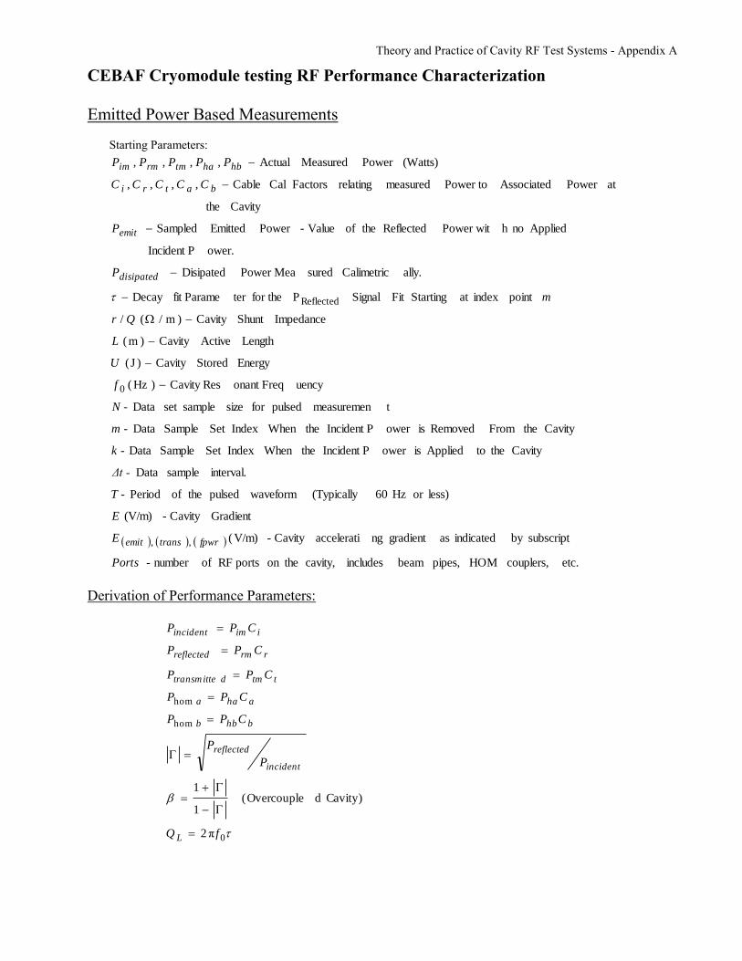
Theory and Practice of Cavity RF Test Systems - Appendix A
CEBAF Cryomodule testing RF Performance Characterization
Emitted Power Based Measurements
Starting Parameters:
etc. couplers, HOMpipes, beam includes cavity, theon ports RFofnumber -
subscriptby indicated asgradient ngacceleratiCavity - V/m)(
GradientCavity -(V/m)
less)or Hz60 (Typically waveformpulsed theof Period
interval. sample Data
Cavity the toApplied isower Incident P theWhenIndex Set Sample Data
Cavity the From Removedisower Incident P theWhenIndex Set Sample Data
tmeasuremen pulsedfor size sampleset Data
uency onant FreqCavity Res )Hz(
EnergyStoredCavity )J(
LengthActiveCavity )m(
ImpedanceShunt Cavity )m/(/
point index at Starting Fit Signal Pfor theter fit Parame Decay
ally.Calimetric sured Power MeaDisipated
ower.Incident P
Applied no h Power wit Reflected theof Value - Power EmittedSampled
Cavity the
at Power Associated Power tomeasured relating FactorsCal Cable ,,,,
(Watts) Power MeasuredActual ,,,,
, ,
0
Reflected
Ports
E
E
T -
Δt -
k -
m -
N -
f
U
L
Qr
m
P
P
CCCCC
PPPPP
fpwrtransemit
disipated
emit
batri
hbhatmrmim
Derivation of Performance Parameters:
0
hom
hom
π2
Cavity)dOvercouple(1
1
fQ
P
P
CPP
CPP
CPP
CPP
CPP
L
incident
reflected
bhbb
ahaa
ttmdtransmitte
rrmreflected
iimincident
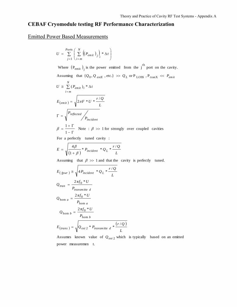
Theory and Practice of Cavity RF Test Systems - Appendix A
CEBAF Cryomodule testing RF Performance Characterization
Emitted Power Based Measurements
t.measuremenpower
emitted an on based typicallyis whichofvalueknownAssumes
/**
*π2
*π2
*π2
/**4
tuned.perfectly iscavity that theand 1thatAssuming
/***
1
4
:cavity tunedperfectly a For
cavities coupledover strongly for 1 :Note 1
1
/**2
*)(
P,or P etc.} ,{ that Assuming
cavity. theonport j thefrom emittedpower theis P Where
*
2
2
hom
0hom
hom
0hom
0
tranXLOSS0
th
jemit
1
ext
dtransm itteexttrans
b
b
a
a
dtransm itte
tran
Lincidentfpwr
Lincident
incident
reflected
emit
N
mi
iemit
emitLextX
Ports
j
N
miijem it
Q
L
QrPQE
P
UfQ
P
UfQ
P
UfQ
L
QrQPE
L
QrQPE
P
P
L
QrUFE
tPU
PQ, QQ
tPU

Theory and Practice of Cavity RF Test Systems - Appendix A
CEBAF Cryomodule testing RF Performance Characterization
Q0 Measurements
CW measurements where Pdissipated is the average dissipated power measured calorimetrically.
dissipateddissipated P
Uf
Qr
L
P
EQ
*π2
/*
0
2
0
For pulsed operation the gradient is not constant throughout the measurement. In this case the
field probe transmitted power is recorded as a function of time with at a sample interval t; the
gradient can be calculated using the transmitted power method; and Q0 is calculated as:
Qr
L
P
tET
Qo
disapated
N
ki
itrans
/*
*1 2
Where Pdissipated is the average dissipated power measured calorimetrically, and T is the period of
the pulses. It should be noted that the numerator in the above equation is used to account for the
non square pulse shape. Values of Q0 calculated using this method will be different for different
gradient pulse shapes or CW operations. If CW values are desired, it is best to make such
measurements with pulse widths that are much greater than the cavity fill times.
To measure the dissipated power calorimetrically one isolates the cryomodule from the helium
supply and return lines and records the rate of rise of the pressure under three conditions. These
are static heat load with RF and resistive heaters on; static plus a known resistive heat load
applied to the bath; and static plus a unknown RF heat load due to the cavity losses. The
dissipated power is then calculated using the following.
.conditionsdifferent under the pressure theof rise of rate theis where
dt
dP
P
dt
dP
dt
dP
dt
dP
dt
dP
P HEATER
STATICONHEATER
STATICONRFDISSIPATED

Theory and Practice of Cavity RF Test Systems - Appendix A
Derivation of Measurement Errors - Cryomodule:
Starting Parameters:
Watts. in in
error theis i.e. variable, theas same theare units The .a variable ofError
tmeasuremenmeter power theoflinearity theofy uncertaint l Fractiona
nscalibratio cable iny uncertaint al Fraction
measuredpower absolute iny uncertaint Fractional
used sensorspower oflimit y Sensitivit min
tran
tran
Lin
cal
P
PΔ
P
C
P
P
Parameter Uncertainties:
22
22
22
homhom
22
homhom
22
22
22
500min
min
min
min
min
min
2
)(
)()()()(
)(
)(
)(
)(
)(
)()()(
incident
incident
reflected
reflected
irm
irmireflectediemit
hbm
bmhbb
ham
amhaa
tm
tmdtransmittedtransmitte
rm
rmreflectedreflected
im
imincidentincident
pwrRFzero
ptsovercalirmirm
calhbmhbm
calhamham
caltmtm
calrmrm
calimim
P
P
P
P
P
PCPP
P
PCPP
P
PCPP
P
PCPP
P
PCPP
P
PCPP
PmeanPPP
PPPP
PPPP
PPPP
PPPP
PPPP

Theory and Practice of Cavity RF Test Systems - Appendix A
22
22
22
min
min
22
2
*4
2
2
floornoisemeterpowertodueisTerm)(
nintegratiothestartingforjittertodueisTerm))((
togintegratinnotfromterm
)()(
transX
transX
transX
transXtranstransX
transX
transX
em it
em itextXextX
incident
incident
L
Lfpwr
fpwr
em item it
r
mem it
N
rNmem itcalr
P
P
Q
QEE
P
P
E
EQQ
P
P
Q
QEE
U
UEE
PCmNt
tP
P
PCmNtPtPPCUU
Where transQ and transQ were entered values that were determined under different
operating conditions and calibrations than the current measurement.
2
min
2**
2
trans
XtransXLin
trans
transtranstrans
P
PCPP
Q
QEE
Where transQ and transQ were determined under same operating conditions and
calibrations than the current measurement.
LinLLL
dissipated
dissipated
trans
transtranstrans
dissipated
dissipated
fpwr
fpwr
fpwrfpwr
PQQQ
P
P
E
EQQ
P
P
E
EQQ
ΔΔ
11
2Δ
2Δ
22
22
)(0)(0
22
)(0)(0

Theory and Practice of Cavity RF Test Systems - Appendix A
CEBAF Vertical Pair Testing RF Performance Characterization
Decay Measurement Formulas
Starting Parameters:
frequency resonant Cavity )Hz(
OFF. d turne
been haspower Fincident R the whenmeasured as signalpower ed transmittor the
signal)power reflected at the measured (as emitted for the (seconds)darameter fit Decay
coupled.over for 1- coupled,under for 1factor coupling Over/under
cavity. at thepower RF
associated power to RFmeasured relating factors ncalibratio Cable ,,,,
tmeasuremendecay for the OFF RF
the turningprior tojust (Watts),power CW RF measured Actual ,,,,
0
f
C
CCCCC
PPPPP
batri
hbhatmrmim
Derivation of Performance Parameters:
0
*
homhom
hom
hom
π2
1
1
fQ
C
P
P
PPPPPP
CPP
CPP
CPP
CPP
CPP
L
incident
reflected
badtransm ittereflectedincidentloss
bhbb
ahaa
ttmdtransm itte
rrmreflected
iimincident
This implicitly assumes that Q0 and the external-Q of all of the RF ports are independent of the
stored energy, i.e. linear, flat Q0 , and constant coupling factor for gradients at or below that of the
starting point of the decay measurement.
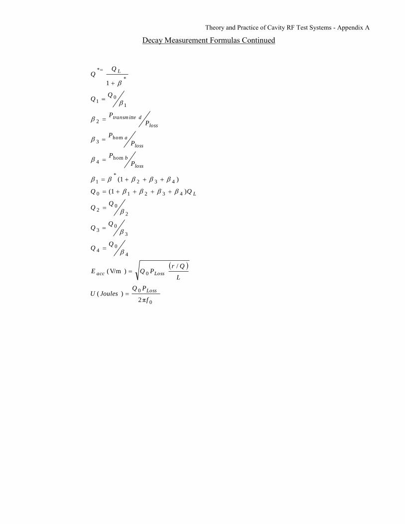
Theory and Practice of Cavity RF Test Systems - Appendix A
Decay Measurement Formulas Continued
0
0
0
4
04
3
03
2
02
43210
432
*
1
hom4
hom3
2
1
01
*
*
π2)(
/)V/m(
)1(
)1(
1
f
PQJoulesU
L
QrPQE
P
P
P
P
P
P
Loss
Lossacc
L
loss
b
loss
a
loss
dtransm itte
L

Theory and Practice of Cavity RF Test Systems - Appendix A
CW Formulas
Starting Parameters:
uency onant FreqCavity Res )Hz(
tmeasuremen Decay previousa from determined as Q External ProbeonTransmissi
OFF. d turne
been haspower Fincident R the whenmeasured as signalpower ed transmittor the
signal)power reflected at the measured (as emitted for the (seconds)darameter fit Decay
coupled.over for 1- coupled,under for 1factor coupling Over/Under
cavity. at thepower RF
associated power to RFmeasured relating FactorsnCalibratio Cable ,,,,
tmeasuremendecay for the OFF RF
the turningprior tojust (Watts), Power CW RF MeasuredActual ,,,,
0
2
f
Q
C
CCCCC
PPPPP
batri
hbhatmrmim
Derivation of Performance Parameters:
b
dtransm itte
a
dtransm itte
loss
dtransm itte
incident
reflected
badtransm ittereflectedincidentloss
bhbb
ahaa
ttmdtransm itte
rrmreflected
iimincident
P
PQQ
P
PQQ
P
PQQ
C
P
P
PPPPPP
CPP
CPP
CPP
CPP
CPP
hom
24
hom
23
1
01
20
*
homhom
hom
hom
1
1
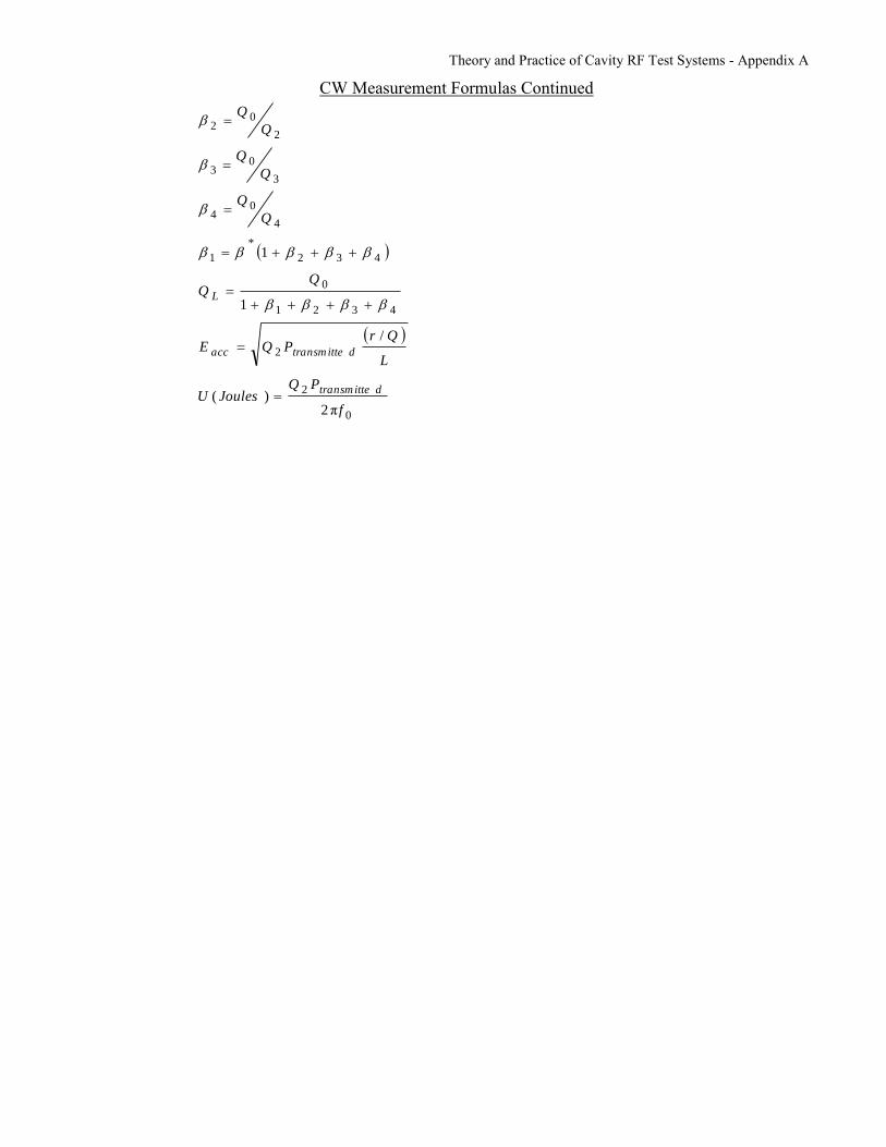
Theory and Practice of Cavity RF Test Systems - Appendix A
CW Measurement Formulas Continued
0
2
2
4321
0
432
*
1
4
04
3
03
2
02
π2)(
/
1
1
f
PQJoulesU
L
QrPQE
Q
Q
Q
Q
Q
Q
dtransmitte
dtransmitteacc
L
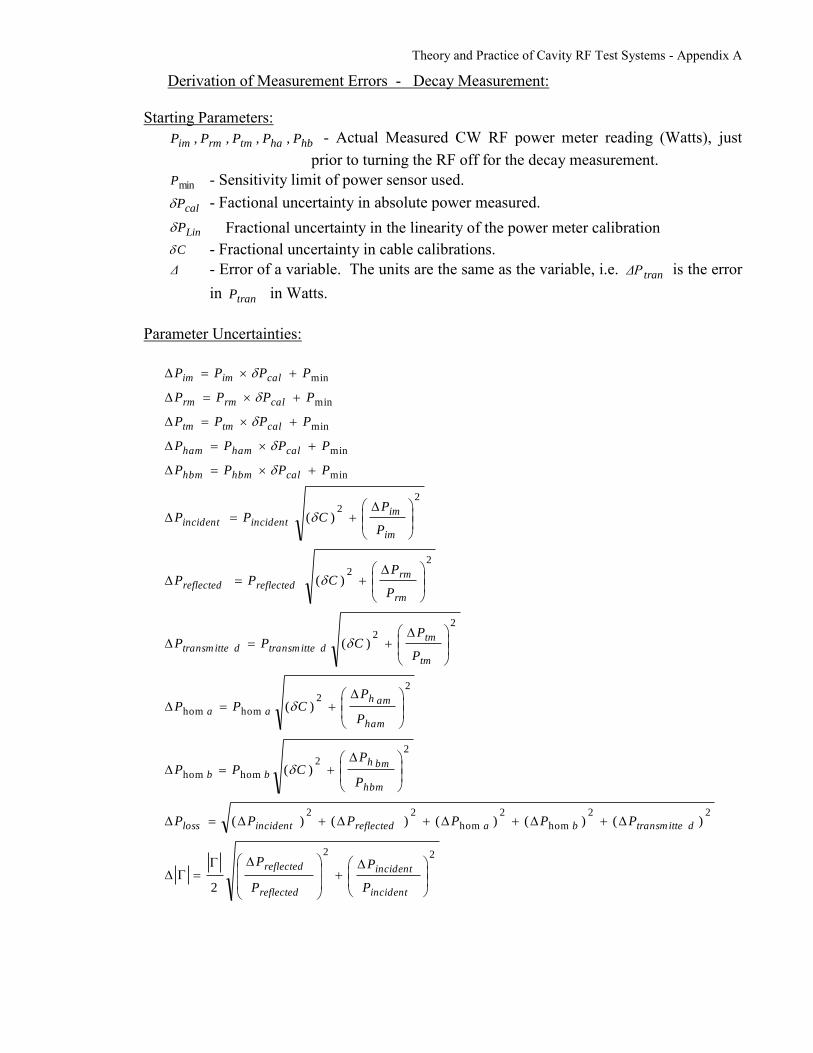
Theory and Practice of Cavity RF Test Systems - Appendix A
Derivation of Measurement Errors - Decay Measurement:
Starting Parameters:
hbhatmrmim PPPPP ,,,, - Actual Measured CW RF power meter reading (Watts), just
prior to turning the RF off for the decay measurement.
minP - Sensitivity limit of power sensor used.
calP - Factional uncertainty in absolute power measured.
LinP Fractional uncertainty in the linearity of the power meter calibration
C - Fractional uncertainty in cable calibrations.
Δ - Error of a variable. The units are the same as the variable, i.e. tranΔP is the error
in tranP in Watts.
Parameter Uncertainties:
22
22
hom
2
hom
22
22
homhom
22
homhom
22
22
22
min
min
min
min
min
2
)()()()()(
)(
)(
)(
)(
)(
incident
incident
reflected
reflected
dtransm ittebareflectedincidentloss
hbm
bmh
bb
ham
amh
aa
tm
tmdtransmittedtransmitte
rm
rmreflectedreflected
im
imincidentincident
calhbmhbm
calhamham
caltmtm
calrmrm
calimim
P
P
P
P
PPPPPP
P
PCPP
P
PCPP
P
PCPP
P
PCPP
P
PCPP
PPPP
PPPP
PPPP
PPPP
PPPP
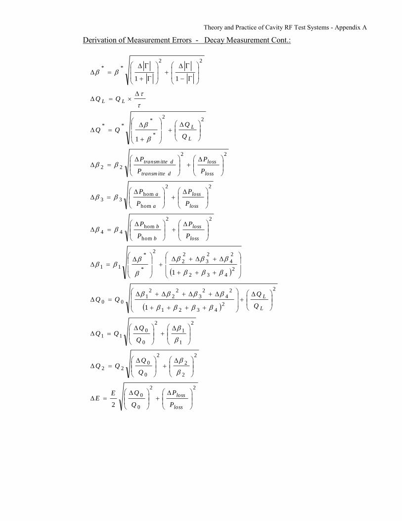
Theory and Practice of Cavity RF Test Systems - Appendix A
Derivation of Measurement Errors - Decay Measurement Cont.:
22
0
0
2
2
2
2
0
022
2
1
1
2
0
011
2
24321
24
23
22
21
00
2432
2
4
2
3
2
2
2
*
*
11
22
hom
hom44
22
hom
hom33
22
22
22
*
***
22
**
2
1
1
1
11
loss
loss
L
L
loss
loss
b
b
loss
loss
a
a
loss
loss
dtransm itte
dtransm itte
L
L
LL
P
P
Q
QEE
Q
QQQ
Q
QQQ
Q
QQQ
P
P
P
P
P
P
P
P
P
P
P
P
Q
QQQ
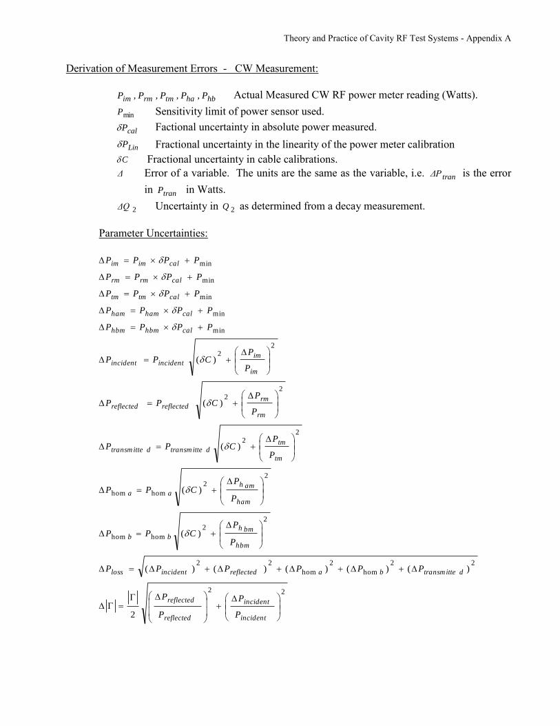
Theory and Practice of Cavity RF Test Systems - Appendix A
Derivation of Measurement Errors - CW Measurement:
hbhatmrmim PPPPP ,,,, Actual Measured CW RF power meter reading (Watts).
minP Sensitivity limit of power sensor used.
calP Factional uncertainty in absolute power measured.
LinP Fractional uncertainty in the linearity of the power meter calibration
C Fractional uncertainty in cable calibrations.
Δ Error of a variable. The units are the same as the variable, i.e. tranΔP is the error
in tranP in Watts.
2ΔQ Uncertainty in 2Q as determined from a decay measurement.
Parameter Uncertainties:
22
22
hom
2
hom
22
22
homhom
22
homhom
22
22
22
min
min
min
min
min
2
)()()()()(
)(
)(
)(
)(
)(
incident
incident
reflected
reflected
dtransmittebareflectedincidentloss
hbm
bmh
bb
ham
amh
aa
tm
tmdtransmittedtransmitte
rm
rmreflectedreflected
im
imincidentincident
calhbmhbm
calhamham
caltmtm
calrmrm
calimim
P
P
P
P
PPPPPP
P
PCPP
P
PCPP
P
PCPP
P
PCPP
P
PCPP
PPPP
PPPP
PPPP
PPPP
PPPP

Theory and Practice of Cavity RF Test Systems - Appendix A
Derivation of Measurement Errors - CW Measurement Cont.:
2
2
2
2
200
loss
lossLin
P
PP
Q
QQQ
0Q error assumes that the 2Q used was measured using the same power meter and cable
calibrations.
222
2
200
loss
loss
tran
tran
P
P
P
P
Q
QQQ
0Q error assumes that the 2Q used was measured using different power meter and cable
calibrations.
22
2
2
24321
24
23
22
21
2
0
0
2
1
1
2
0
011
2432
24
23
22
2
11
22
**
2
4
4
2
0
044
2
3
3
2
0
033
2
2
2
2
0
022
22
hom
hom
2
2
244
22
hom
hom
2
2
233
2
1
1*
*
11
dtransm itte
dtransm itte
LL
loss
loss
b
b
loss
loss
a
a
P
P
Q
QEE
Q
QQQ
Q
QQQ
Q
Q
Q
Q
Q
Q
Q
Q
Q
Q
Q
Q
P
P
P
P
Q
QQQ
P
P
P
P
Q
QQQ