Theory and Application of Induced

Higher Order Color Aberrations

Dissertationzur Erlangung des akademischen Grades

Doktor-Ingenieur (Dr.-Ing.)

vorgelegt dem Rat der Physikalisch-Astronomischen Fakultät

der Friedrich-Schiller-Universität Jena

von M.Eng. Andrea Berner

geboren am 10.09.1986 in Nordhausen

Gutachter

1. Prof. Dr. Herbert Gross, Friedrich-Schiller-Universität Jena

2. Prof. Dr. Alois Herkommer, Universität Stuttgart

3. Prof. Dr. Burkhard Fleck, Ernst-Abbe-Hochschule Jena

Tag der Disputation: 09.06.2020

Contents

1 Motivation and Introduction 5

2 Theory and State of the Art 82.1 Paraxial Image Formation . . . . . . . . . . . . . . . . . . . . . . . . . 8

2.1.1 Paraxial Region . . . . . . . . . . . . . . . . . . . . . . . . . . . 82.1.2 Paraxial Properties of an Optical Surface . . . . . . . . . . . . . 92.1.3 Paraxial Raytrace and Lagrange Invariant . . . . . . . . . . . . 112.1.4 Refractive Power of a Thick and a Thin Lens . . . . . . . . . . . 13

2.2 Aberration Theory . . . . . . . . . . . . . . . . . . . . . . . . . . . . . 152.2.1 Wavefront Aberration Function . . . . . . . . . . . . . . . . . . 152.2.2 Transverse Ray Aberration Function . . . . . . . . . . . . . . . 202.2.3 Seidel Surface Coefficients . . . . . . . . . . . . . . . . . . . . . 21

2.3 Chromatic Aberrations . . . . . . . . . . . . . . . . . . . . . . . . . . . 232.3.1 Axial Color Aberration . . . . . . . . . . . . . . . . . . . . . . . 262.3.2 Lateral Color Aberration . . . . . . . . . . . . . . . . . . . . . . 28

2.4 Design Process . . . . . . . . . . . . . . . . . . . . . . . . . . . . . . . 302.5 State of the Induced Aberration Problem . . . . . . . . . . . . . . . . . 32

2.5.1 Induced Monochromatic Aberration . . . . . . . . . . . . . . . . 332.5.2 Induced Axial and Lateral Color . . . . . . . . . . . . . . . . . . 342.5.3 Induced Chromatic Variation of 3rd-order Aberrations . . . . . 35

3 Extended Induced Color Aberration Theory 363.1 The Concept of Induced Color Aberrations . . . . . . . . . . . . . . . . 36

3.1.1 Characteristics . . . . . . . . . . . . . . . . . . . . . . . . . . . 363.1.2 Aberration Classification . . . . . . . . . . . . . . . . . . . . . . 373.1.3 Overview of new Results in this Chapter . . . . . . . . . . . . . 38

3.2 Induced Axial Color . . . . . . . . . . . . . . . . . . . . . . . . . . . . 393.2.1 Surface Contribution of Intrinsic and Induced Axial Color . . . 393.2.2 Lens Contribution of Intrinsic and Induced Axial Color . . . . 433.2.3 Discussion . . . . . . . . . . . . . . . . . . . . . . . . . . . . . . 45

3.3 Induced Lateral Color . . . . . . . . . . . . . . . . . . . . . . . . . . . 47

3

3.3.1 Surface Contribution of Intrinsic and Induced Lateral Color . . 473.3.2 Lens Contribution of Intrinsic and Induced Lateral Color . . . . 533.3.3 Discussion . . . . . . . . . . . . . . . . . . . . . . . . . . . . . . 55

3.4 Induced Spherochromatism . . . . . . . . . . . . . . . . . . . . . . . . . 583.4.1 Definition of Spherochromatism . . . . . . . . . . . . . . . . . . 583.4.2 Surface Contribution of Intrinsic and Induced Spherochromatism 603.4.3 Thin Lens Contribution of Intrinsic and Induced Spherochromatism 653.4.4 Discussion . . . . . . . . . . . . . . . . . . . . . . . . . . . . . . 67

3.5 Induced Chromatic Variation of 3rd-order Seidel Aberrations . . . . . . 70

4 Application of the New Theory 734.1 Classical Design Examples . . . . . . . . . . . . . . . . . . . . . . . . . 73

4.1.1 8f-imaging System . . . . . . . . . . . . . . . . . . . . . . . . . 734.1.2 Thick Meniscus . . . . . . . . . . . . . . . . . . . . . . . . . . . 774.1.3 Schupmann Achromat . . . . . . . . . . . . . . . . . . . . . . . 784.1.4 Catadioptric System . . . . . . . . . . . . . . . . . . . . . . . . 814.1.5 Split Achromat . . . . . . . . . . . . . . . . . . . . . . . . . . . 84

4.2 Complex Design Example - A Microscope Objective Lens . . . . . . . . 894.2.1 Design Specifications . . . . . . . . . . . . . . . . . . . . . . . . 894.2.2 Design Analysis . . . . . . . . . . . . . . . . . . . . . . . . . . . 924.2.3 Improved Analysis by the New Theory . . . . . . . . . . . . . . 94

5 Summary 102

A Appendix i

Bibliography vii

List of Figures xii

List of Tables xiv

Zusammenfassung

Ehrenwörtliche Erklärung

Danksagung

4

1 Motivation and Introduction

Optical design describes an optimization process for lens systems combining appliedaberration theory, system engineering and the experience of the designer. Meeting aset of optical performance specifications as well as manufacturing and costs constraints,very often complex lens systems with a multi-dimensional solution space are required.Prior to the development of digital computers, lens optimization was a hand-calculationtask using trigonometric and logarithmic tables to calculate selected single rays trougha lens system up to the image. Nowadays, for this purpose, the main tool of an opticaldesigner is the computer. Since computational power became available, the empha-sis quickly shifted to powerful optimization techniques. They can navigate the designthrough the multi-dimensional solution space and push it to different local minima. Toevaluate the several found solutions, a merit function is set up by the optical designer.Ensuring the final performance at the end of the optical system, typically this meritfunction is based on ray intersection operands at the final image plane and on some1st-order parameters, e.g. focal length, magnification or intersection length. An ex-plicit control of certain 3rd-order or even higher-order aberrations is unusual to givemeaningful measures of the final image quality. Hence, because of the ability to domany computations simultaneously and due to the associated tendency to treat lenssystems as black boxes, a deeper understanding about how and why a lens design workscan only be achieved by a systematic and constant analysis of the different optimizeddesign states.The best way to find out the inner workings of an optical systems is to understandwhy aberrations arise and how they sum up surface by surface to their final amountat the image plane. Such a surface or lens resolved analysis describes the key methodfor achieving a deeper understanding and better optimizations of the designs. Its mainadvantage is the identification of performance dominating surfaces or lenses, refer-ring to the five primary, 3rd-order aberrations, which are spherical aberration, coma,astigmatism, field curvature and distortion as well as to the chromatic aberrations.Furthermore, well balanced aberration contributions additionally indicate the systeminsensitivity to large tolerances, which always is an intended characteristic of a goodlens design. Ludwig Seidel [Sei56] derived these well-known coefficients in 1856 andestablished the basic principles of aberration correction. Knowing the single contribu-

5

tions of every lens within the optical system enables the designer to work with deter-mined steps like decreasing ray angles at dominating surfaces, add lenses at stressedpositions or changing glasses of lenses with less or inverted chromatic contributions.Re-optimization after such determined system changes can push the design quickly tobetter or simpler states.As today a multitude of the lens designs are specified to work in broad wavelengthranges, providing large field of views and apertures within very compact lens dimen-sions, higher-order aberrations are often the factor that at the end limits the resolutiona lens can give [KT02]. Hence, although the correction of the five 3rd-order aberrationsand the 1st-order chromatic aberration is a necessary condition to guarantee a goodoverall aberration correction, the influence of higher-order aberrations can not be ne-glected in all cases. Assuming the same ray-based approach like Seidel, Buchdahl andRimmer[Buc54], [Rim63] derived the 5th- and 7th-order surface contributions of themonochromatic aberrations in 1963. Hoffman [Hof93] and Sasian [Sas10] completed5th-order surface contribution theory in terms of wavefront aberration in 1993 and2010. Clearly, those coefficients are not that reasonably simple anymore, but they arewell described and discussed today.In contrast to the 3rd-order aberrations, which are completely independent of eachother, 5th-order aberrations are characterized by additional aberration parts that areinduced by prior generated aberrations of lower-order. This special differentiation be-tween induced and intrinsic contributions allows the lens designer not only to analyze,if there are dominating 5th-order aberrations, but it also tells how well the intrinsic andinduced parts are balanced. Thereby, large induced aberrations parts refer to eitherunbalanced great 3rd-order aberrations somewhere inside the system or in some spe-cial cases large induced contributions even helps to correct the remaining intrinsic parts.

The present investigation now applies to the induced surface contributions of coloraberrations. Especially for today’s advanced applications, different challenges regard-ing the chromatic correction of optical systems have to be managed. For instance, incase of consumer optics, where mostly only plastic lenses can be applied because ofweight and cost specifications, or in case of freeform optics, where the overall numberof optical elements is often limited by compactness requirements, the options for colorcorrection regarding glass choice and an appropriate refractive power distribution arehighly restricted. Other applications, like hyper spectral imaging systems, IR- and Ra-man microscopy, again have to cover and correct an extreme broad wavelength bandby the optical elements of the systems. Hence, for these cases the lens designer hasto go further than the classical 1st-order color correction of axial and lateral colorby considering also higher-order color aberrations and by taking advantage of inducedaberration effects. To enable the designer to understand and to push its optical system

6

concerning these aberrations, the new expressions for induced surface contributions ofcolor aberrations were derived in this investigation.In contrast to the monochromatic aberrations, here, induced influences are alreadyobservable in the paraxial regime, since even paraxial rays are affected by dispersion.In analogous manner, lower-order aberrations picked up surface by surface in the pre-ceding optical system, generates induced aberrations of higher order. In case of axialcolor and lateral color, different orders refer to the dependency of paraxial rays on dis-persion. Concerning the chromatic variation of 3rd-order aberrations, different ordersrefer to the dependency of monochromatic 3rd-order aberrations on 1st-order coloraberrations. In overcoming the analytical gap discussed in Section 2.5 for inducedsurface contributions of color aberrations in literature, the derivations for both caseswill be given in this investigation. Spherochromatism as the most significant and mostdiscussed chromatic variation of 3rd-order aberration is particularly emphasized. Fi-nally, five classical and academic examples for induced color aberrations as well as onecomplex microscope lens design will be analyzed extensively. Here, the new theory isapplied, in order to understand how the higher-order color aberrations behave in realoptical systems and to demonstrate how their induced and intrinsic aberration partscan influence the overall performance of the optical system.

7

2 Theory and State of the Art

2.1 Paraxial Image Formation

The paraxial approximation of imaging considers the properties of light only in theregion infinitesimally close to the optical axis. This area is usually known as theparaxial region or the Gaussian region. Inside this, all paraxial rays starting at onepoint 𝑂(𝑥, 𝑦) of the object plane 𝑂𝑃 will perfectly meet at an image point 𝑂′(𝑥′, 𝑦′)

at the conjugated paraxial image plane 𝐼𝑃 . Figure 2-1 shows this main concept ofparaxial imaging.

Figure 2-1: Paraxial approximation of imaging, assuming all rays starting at onepoint of the object plane 𝑂𝑃 perfectly meeting at an image point of theconjugated image plane 𝐼𝑃 .

2.1.1 Paraxial Region

The domain of paraxial rays is valid, if they are close enough to the optical axis toensure that all terms of higher order of magnitude than quadratic in heights and inangles are to be neglected. Hence, to define the paraxial region, three assumptionshave to be taken into account. Initially, any refracting or reflecting surface with an

8

curvature of c can be described by the first term in power series of a spherical surfacesag z :

𝑧 ≈ 1

2𝑐𝑦2 (2.1)

Furthermore, the extension of the object and the image surfaces in x- and y-coordinatesare limited to terms proportional to the square of the real object and image size. Finally,any ray angle is assumed to be sufficiently small so that its sine and the tangent functioncan also be linear approximated by[KT02]:

sin 𝑖 ≈ tan ≈ 𝑖 (2.2)

The cosine function is set equal to 1 in this approximation.Although these assumptions limit the validity of the paraxial approach to a very smallarea enclosing the optical axis, the paraxial approximation enables the calculation ofthe basic properties of an optical system like working distance, total track length, theLagrange Invariant as well as the entrance and exit pupil positions. Even the estimationof the system performance based on paraxial relationships are of tremendous utility.Their simplicity makes calculation and manipulation quick and easy. Optical systemsof practical value forming good images, apparently show that most of the light raysoriginating at an object point must pass at least reasonably close to the paraxial imagepoint. Hence, the image point locations given by the paraxial relationships serve asan excellent approximation for the imaging of a well-corrected optical system [Smi66].For this reason, paraxial imaging represent the point of reference for the definition ofall aberrations.

2.1.2 Paraxial Properties of an Optical Surface

For the present investigation in this work, especially the surface related paraxial rela-tions will be of greater interest. Figure 2-2 shows the imaging of an optical surface byrefraction, assuming rotational symmetry along the z-axis. Please note, the marginalray is defined as the paraxial ray starting at the optical axis passing through the edgeof the aperture stop. The chief ray is defined as the ray starting at the maximumobject height, passing through the center of the aperture stop.The refractive spherical surface has a radius R with a center of curvature at c andseparates two media of refractive index 𝑛 and n’ in front and behind, respectively. Themarginal ray intersects the surface at a ray height y. Its incident ray encloses the angleu with the axis before refraction and u’ after refraction. The angle i describes theangle between the incident marginal ray and the normal to the surface and the anglei’ is the angle between the refracted ray and the normal. Please note, all of the abovedescribed ray parameters similarly apply for the chief ray. Those quantities are labeled

9

with bars. The distance of the object is denoted by the intersection length s and itsheight by 𝑦𝑂. After imaging through the surface, the image arises at an intersectionlength of s’ and its height is 𝑦𝐼 .

Figure 2-2: Refraction at an optical surface, assuming rotational symmetry alongz-axis.

Generally, the normal Cartesian sign convention is applied, including these extensions:

• Light travels from left to right in 𝑧-direction.

• Ray heights above the optical axis are positive and under the optical axis arenegative.

• Distances to the right of the surface are positive and to the left are negative.

• A radius is positive if the center of curvature lies to the right of the surface.

• Ray angles are positive if the slopes of the rays are positive.

• The angles of incidence and refraction are positive if the ray is rotated clockwiseto reach the normal.

Determining the ray path from surface to surface through the optical system, Snell’slaw of refraction at dielectric interfaces or mirrors, 𝑛 sin 𝑖 = 𝑛′ sin 𝑖′, has to be applied[Gro+07]. Following Equation 2.2, in paraxial approximation this is written as

𝑛𝑖 = 𝑛′𝑖′ (2.3)

Furthermore, simple trigonometric considerations reviewing Figure 2-2 concerning theray angles u and u’ as well as the marginal incident angle i and the emergent angle i’lead to (2.4).

𝑢′ = 𝑢− 𝑖 + 𝑖′ (2.4)

𝑖 = 𝑢 + 𝑦𝑐 (2.5)

10

𝑖′ = 𝑢′ + 𝑦𝑐 =𝑛𝑖

𝑛′ (2.6)

By equivalent trigonometric treatment of the ray height y and the intersection lengthss as well as s’, Equations (2.7) and (2.8) are obtained.

𝑢 = −𝑦

𝑠(2.7)

𝑢′ = − 𝑦

𝑠′(2.8)

Now, if the two relations (2.3) and (2.4) as well as the paraxial approximation of (2.1) isassumed, the imaging equation of 2.9 for a refracting spherical surface can be deduced[Smi66].

𝑛′

𝑠′− 𝑛

𝑠= (𝑛′ − 𝑛)𝑐 = 𝐹 (2.9)

Here, F is the refractive power of the surface. A surface with positive power will benda ray toward the axis and a negative-powered surface will bend a ray away from theaxis.

2.1.3 Paraxial Raytrace and Lagrange Invariant

Paraxial Raytrace If now calculations are to be continued through more than onesurface, paraxial ray tracing is required. Reviewing the imaging equation of (2.9) andrearranging it by separating quantities before refraction and quantities after refraction,the following relation is obtained:

𝑛′

𝑠′=

𝑛

𝑠+ (𝑛′ − 𝑛)𝑐 (2.10)

Multiplying both sides of the equation by y leads to

𝑛′𝑦

𝑠′=

𝑛𝑦

𝑠+ (𝑛′ − 𝑛)𝑦𝑐 (2.11)

and by substituting 𝑦/𝑠 and 𝑦/𝑠′ according to Equation (2.7) and (2.8), the relationdescribing the ray angle u’ after refraction at a single spherical surface yields:

𝑛′𝑢′ = 𝑛𝑢− 𝑦𝑐(𝑛′ − 𝑛) = 𝑛𝑢− 𝑦𝐹 (2.12)

To continue the calculation to the next surface of the system, a set of transfer equationsare required. Figure 2-3 shows two spherical surfaces, 𝑗 and 𝑗+1, of an arbitrary opticalsystem separated by an axial distance d. The ray is shown after refraction by surface𝑗; its slope is the angle 𝑢′

𝑗. The intersection heights of the ray at the surfaces are 𝑦𝑗

11

and 𝑦𝑗+1, respectively.

Figure 2-3: Paraxial ray transfer at an arbitrary surface 𝑗 ofan optical system to surface 𝑗 + 1.

The triangle formed by the distance d and both ray intersection points results in thetrigonometric relation:

tan𝑢′𝑗 =

𝑦𝑗 − 𝑦𝑗+1

𝑑(2.13)

Within the paraxial approximation and by rearranging to obtain the ray height at thesecond surface 𝑗 + 1, this relation simplifies to:

𝑦𝑗+1 = 𝑦𝑗 + 𝑑𝑢′𝑗 (2.14)

Since the slope of the ray incident on surface 𝑗 + 1 is the same as the slope afterrefraction by surface 𝑗, a second transfer equation is achieved:

𝑛′𝑗𝑢

′𝑗 = 𝑛𝑗+1𝑢𝑗+1 (2.15)

Therefore, only the two Equations (2.12) and (2.14) are necessary to calculate a raytraceof any paraxial ray through an arbitrary optical system up to the image plane [Smi66].Please note, if the marginal ray is chosen, like exemplary did in the equations above,the position of the image formed by the complete optical system can be determinedand if the chief ray is chosen, the image size is obtained.

Lagrange Invariant A second important concept in paraxial optics, should also beemphasized here, since it is fundamental in calculating the 3rd-order aberrations, theLagrange Invariant H. Reviewing the raytrace Equation (2.12) for the marginal ray,the same can be applied for the chief ray:

𝑛′�̄�′ = 𝑛�̄� + 𝑦𝑐(𝑛′ − 𝑛) = 𝑛�̄� + 𝑦𝐹 (2.16)

12

Here, the barred ray parameters refer to the chief ray. By eliminating 𝑐(𝑛′−𝑛) in bothequations, the following relation, known as the Lagrange Invariant or optical invariantat spherical surfaces is obtained:

𝑛(𝑢𝑦 − �̄�𝑦) = 𝑛′(𝑢′𝑦 − �̄�′𝑦) = 𝐻 (2.17)

Since it is also invariant after transfer from one surface to another, the relation isidentical at all surfaces in a lens system. It can be shown that the square of theLagrange Invariant is proportional to the energy transmitted by the lens, assumingthat the object radiates uniformity [KT02]. Hence, the Lagrange Invariant can beunderstood as a consequence of the law of conversation of energy in refracting opticalsystems [Wel86].

2.1.4 Refractive Power of a Thick and a Thin Lens

The refractive power F of an optical element is defined as the reciprocal of its effectivefocal length f. In general, the focal length of an optical system can simply be calculatedby tracing a ray through the optical system, coming from infinity, with an initial rayangle u equal to zero. The effective focal length then is defined as the relation of theray height at the first surface and the ray angle after emerging from the last surface.Similarly, for the back focal length the ray height at the last surface is taken intoaccount. In a system with k surfaces, Equation (2.18) and (2.19) show the definitionsof the effective focal length f and the back focal length f ’, respectively[Smi66].

𝑓 = − 𝑦1𝑢′𝑘

(2.18)

𝑓 ′ = −𝑦𝑘𝑢′𝑘

(2.19)

Assuming now a thick lens in air, having a refractive index of n, the effective focallength can easily be calculated by tracing a parallel ray through the two surfaces ofthe thick lens. The surface radii are 𝑅1 and 𝑅2 and the surface curvatures are 𝑐1 and𝑐2. The lens’ thickness is 𝑡. Figure 2-4 illustrates these relevant quantities for the thicklens approach. If the lens is surrounded by air, the indices of refraction can be assumedto be 𝑛0 = 𝑛2 = 1.

13

Figure 2-4: Refraction of the marginal ray (solid line) and the chief ray(dashed line) at a thick lens.

Applying the raytrace equations of Subsection 2.1.3, the refractive power 𝐹 𝑡𝐿 of a thicklens, or the reciprocal of its effective focal length, can now be expressed by [Smi66]:

𝐹 𝑡𝐿 =1

𝑓= −𝑢2

𝑦1

= (𝑛− 1)

(︂𝑐1 − 𝑐2 + 𝑡𝑐1𝑐2

𝑛− 1

𝑛

)︂

= (𝑛− 1)

(︂1

𝑅1

− 1

𝑅2

+𝑡(𝑛− 1)

𝑛𝑅1𝑅2

)︂(2.20)

Referring to the definition of the refractive power of a single surface, as shown in (2.9),the refractive power of a thick lens can also be calculated by considering the singlesurface powers 𝐹1 and 𝐹2 and the thickness t :

𝐹 𝑡𝐿 = 𝐹1 + 𝐹2 −𝑡𝐹1𝐹2

𝑛(2.21)

Reviewing this relation, also an equivalent expression for thin lenses can be found.By considering the limiting behavior of Equation (2.20) for t converging to zero, therefractive power 𝐹𝐿 of a thin lens is described by:

𝐹𝐿 = (𝑛− 1) (𝑐1 − 𝑐2)

= (𝑛− 1)

(︂1

𝑅1

− 1

𝑅2

)︂

= 𝐹1 + 𝐹2 (2.22)

14

2.2 Aberration Theory

In Section 2.1 the perfect imaging characteristics of optical systems, limited to aninfinitesimal close region to the optical axis, were discussed. Here, a lens forms animage without any aberrations. The image size as well as the location are given by theequations for the paraxial region. Leaving this paraxial region of an imaging system, ingeneral, real optics with finite ray heights and ray angles do not perform ideal imaging.Hence, rays emerging from one object point O(x,y) will not all perfectly meet at asingle image point O’(x’,y’). Figure 2-5 shows an example with three random rays ofthe y-z-plane.

Figure 2-5: Real imaging of an optical system, considering real optics with finite rayheights and ray angles.

To determine the aberrations by the amount by which the real rays miss the paraxialimage point, several methods are used for description. Deviations from perfect imagingcan either be described in terms of wavefront aberrations, measured in optical pathlength differences, or in terms of the geometrical ray interception errors, measured intransverse or longitudinal aberrations at the image plane.

2.2.1 Wavefront Aberration Function

Wavefront Definition The fundamental law for defining wavefront aberrations isthe theorem of Malus and Dupin. It states the definition of a wavefront by a surfaceof constant optical path length measured from a point at the object plane. Figure 2-6illustrates this principle. Here, several rays are traced from a source point O at theobject plane. The points 𝑃1, 𝑃2 and 𝑃3 all represent points, having the same opticalpath length |𝑂𝑃1| = |𝑂𝑃2| = |𝑂𝑃3| starting at O. This is also true for any other rayoutside the y-z-plane starting at O. In case of an isotropic material having a refractiveindex of n, the wavefront is the locus of the points 𝑃1, 𝑃2, 𝑃3 etc., since it representsthe surface of constant optical path length. Please note, the wavefront containing the

15

points 𝑃1 up to 𝑃𝑛 is a sphere centered on O. However, if the points 𝑄1 up to 𝑄𝑛 ofthe image space are taken, the wavefront is not in general a sphere anymore, since itwas aberrated by the preceding optical system [KT02]. Here, it is easy to see, that thetheorem of Malu and Dupin can also be interpreted in such a way that geometricalwavefronts always are perpendicular to the rays starting at the same object point[Wel86].

Figure 2-6: Definition of wavefronts as a surface of constant optical path lengthmeasured from a point at the object plane.

Wavefront Aberration After describing the wavefront itself, a definition for thewavefront errors is introduced. Spherical wavefronts in image space converge to asingle, unblurred image point. However, aberrated wavefronts deviate from a perfectsphere. Therefore, it is suitable to express the wavefront aberration W with respectot a reference sphere. It is measured in terms of optical path length difference alongthe ray. In general, the reference sphere is determined by its center O’, which is theassumed paraxial image point, and by its radius R. Usually, R is defined by the locationof the exit pupil, so that the reference sphere contains the intersection point of the chiefray with the optical axis. Figure 2-7 illustrates these conditions.

16

Figure 2-7: Wavefront aberration defined as the deviation of the wavefront to a ref-erence sphere (dotted line). This is determined by the paraxial imagepoint O’ as center and the intersection point of the chief ray with theoptical axis.

By considering the definition of the wavefront aberration W, the optical path measuredalong the ray from the reference sphere to the wavefront is obtained by [Gro+07]:

𝑊 = [𝑂𝑄2] − [𝑂𝐽2] (2.23)

In this case, the wavefront aberration is negative, 𝑊 < 0.

Power Series Expansion The example above shows, that the wavefront aberrationclearly depends on the chosen ray. If the wave aberration is to be described for all raysemerging from the object point O and passing through the exit pupil, all concernedrays can be identified by their pupil coordinates 𝑥𝑝 and 𝑦𝑝. Hence, the wave aberra-tion 𝑊 (𝑥𝑝, 𝑦𝑝) then becomes a function of two variables. However, this function onlydescribes the aberrations for the chosen object point O. A complete information aboutthe total system aberrations is only obtained by considering the whole object field.Therefore, if an object point is characterized by its object plane coordinates x and y,then the wavefront aberration becomes a function of four variables 𝑊 (𝑥, 𝑦, 𝑥𝑝, 𝑦𝑝). Thisfunction of four variables is essential, if optical systems without rotational symmetryare investigated [Gro+07]. For reasons of simplification, Figure 2-8 only shows theobject plane and the exit pupil plane of an optical system.Here, a single ray is regarded, starting at the object coordinates x and y and passingthrough the pupil coordinates 𝑥𝑝 and 𝑦𝑝. For this ray the wavefront aberration is definedby 𝑊 (𝑥, 𝑦, 𝑥𝑝, 𝑦𝑝). In the more common case of a rotational symmetric system, thisray can be rotated about the optical axis by an arbitrary amount, but the wavefrontaberration will still be the same.

17

Figure 2-8: Definition of field vector 𝐹 at the object plane and pupil vector𝑃 at the pupil plane of an optical system.

Hence, instead of describing the ray by the above mentioned four variables of theCartesian object and pupil coordinates, adapted variables which are invariant withrespect to rotation about the optical axis, can be found. Consequently, if 𝐹 indicatesthe field vector within the object plane origin to the object point (x, y) and if 𝑃 isthe pupil vector from the pupil plane origin to the pupil point (𝑥𝑝, 𝑦𝑝), the rotationalinvariant variables are:

|𝐹 |2 = 𝑥2 + 𝑦2 the square of the field vector length

|𝑃 |2 = 𝑥2𝑝 + 𝑦2𝑝 the square of the pupile vector length

𝑃 · 𝐹 = |𝑃 ||𝐹 | cos(𝜙) = 𝑥𝑝𝑥 + 𝑦𝑝𝑦 the scalar product of 𝑃 and 𝐹

In addition to the lengths of both vectors, the last quantity also contains the infor-mation about the angle 𝜙 = 𝜙𝐹 − 𝜙𝑃 between the two vectors. With these new rota-tional invariant variables the wavefront aberration for an arbitrary ray can be stated as𝑊 (𝑥2 + 𝑦2 , 𝑥2

𝑝 + 𝑦2𝑝 , 𝑥𝑝𝑥+ 𝑦𝑝𝑦), depending only on the length of the object vector, thelength of the pupil vector and on the angle between the object and pupil vector. Now,without loss of generality, one more simplification can be assumed as the object pointcan be chosen to lay on the y-axis. Therefore, by setting 𝑥 = 0 the wave aberrationthen is defined by [Gro+07]:

𝑊 (𝑦2, 𝑥2𝑝 + 𝑦2𝑝, 𝑦𝑝𝑦) (2.24)

An equivalent and also often used expression for W is found by changing from Cartesiancoordinates to a polar coordinate description. In this case, the field coordinate y stays

18

the same, as it was chosen to lay on the y-axis . For the pupil parameters, the radialcoordinate r is assumed to be 𝑟2 = 𝑥2

𝑝 + 𝑦2𝑝 and the angular coordinate is defined bycos𝜙 = 𝑦𝑝/𝑟. Hence, in polar coordinates the wavefront aberration function reads:

𝑊 (𝑦2, 𝑟2, 𝑦 𝑟 cos𝜙) (2.25)

To classify now the different types of image errors comprised by the wavefront aberra-tion function and to understand the behavior of each type, W can be written in themost general power series of its three variables. The result is shown in Equation (2.26).Here, again polar coordinates were assumed.

𝑊 = 𝑊 (𝑦, 𝑟, 𝜙)

= + 𝑤020𝑟2 + 𝑤111𝑦𝑟 cos𝜙 Defocus and scale error

+ 𝑤040𝑟4 + 𝑤131𝑦𝑟

3 cos𝜙 + 𝑤222𝑦2𝑟2 cos2 𝜙 Primary aberrations

+ 𝑤220𝑦2𝑟2 + 𝑤311𝑦

3𝑟 cos𝜙

+ 𝑤060𝑦6 + 𝑤151𝑦𝑟

5 cos𝜙 + 𝑤242𝑦2𝑟4 cos2 𝜙 Higher-order aberrations

+ 𝑤240𝑦2𝑟4 + 𝑤331𝑦

3𝑟3 cos𝜙 + 𝑤333𝑦3𝑟3 cos3 𝜙

+ 𝑤422𝑦4𝑟2 cos2 𝜙 + 𝑤420𝑦

4𝑟2 + 𝑤511𝑦5𝑟 cos𝜙

(2.26)Please note, since a power expansion is strictly mathematical, but the wavefront aber-ration is not an arbitrary function to be expanded, a constant term and all coefficientswith no dependence on pupil parameters were set to zero within this mathematicalexpression [Gro+07]. The latter is due to the fact that those wavefront parts are as-sociated to the chief ray and therefore would cause 𝑊 (𝑦, 𝑟, 𝜙) to be zero for this point[Hop50].Equation (2.26) now shows the classification of the different aberrations types. Thecoefficient’s notation by 𝑤𝑖,𝑗,𝑘, which is due to Hopkins [Hop50], indicate the nature ofthe different aberrations by their suffixes, concerning on how they depend on the field,which is the first suffix, on the pupil, which is the second suffix, as well as in whichpower they depend on the azimuth angle 𝜙, described by the third suffix. However, theclassification to primary and higher-order aberrations is only based on their dependenceon the field coordinate y and the aperture coordinate 𝑟. Considering this, in axiallysymmetrical systems, the sum of field and pupil powers only gives even-order terms.Odd-order terms may not exist. Therefore, primary aberrations include all terms thatare dependent on the fourth power in field and aperture and higher-order aberrationsshow a total power sum of sixth-, eighth- and tenth-order etc. The defocus and thescale error, are usually not considered as aberrations at all, since those terms do notprohibit perfect imaging. Defocus only shifts the perfect image to another image plane

19

in 𝑧-direction and the magnification error generates a perfect image but of differentsize.To specify the primary aberration more detailed, the five terms shown in Equation(2.26) are spherical aberration, coma, astigmatism, field curvature and distortion, re-spectively. The spherical aberration term 𝑤040𝑟

4 is the only one, which is independentof the object size y and the azimuth angle 𝜙, so it is constant over field and azimuthangle. Expressed as a wavefront aberration, it is proportional to 𝑟4 and therefore theonly monochromatic aberration that can occur on-axis. However, coma, 𝑤131𝑦𝑟

3 cos𝜙,is proportional to 𝑟3 in the y-z section, but within the x-z-section, when 𝑦𝑝 = 0 andcos𝜙 = 0 , this wavefront aberration is zero. Since coma is linearly proportional to y,at small field angles coma is the most important off-axis aberration. In contrast, thewavefront aberrations associated with astigmatism and field curvature, 𝑤222𝑦

2𝑟2 cos2 𝜙

and 𝑤220𝑦2𝑟2 respectively, are both proportional to 𝑟2. Hence, these aberrations gen-

erate a defocus effect of some extent. Specifically, the field curvature term representsa defocus that is proportional to 𝑦2 and therefore causes a curved image plane andcorresponding to this, astigmatism is a similar aberration, but it is purely cylindrical.Therefore, astigmatism gives only a defocus for the tangential section. The fifth pri-mary aberration is distortion,𝑤311𝑦

3. Comparable to the scale error, distortion alsoproduces a lateral displacement of the image, but in this primary aberration case itadditionally varies with field y and is proportional to the third power of it [KT02].

2.2.2 Transverse Ray Aberration Function

The transverse ray aberration ∆𝑥′ and ∆𝑦′ give the lateral displacement componentsin 𝑥- and 𝑦-direction of the ray intersection point with a reference plane measured froma reference point. Usually, the paraxial image plane and the intersection point of chiefray are used for these references. Figure 2-9 illustrates the transverse ray aberrationin the 𝑦-𝑧-plane of an optical system.

Figure 2-9: Transverse ray aberration Δ𝑦′ in the y-z-plane of an opticalsystem.

20

According to Equations (2.27) and (2.28) the transverse ray aberrations can be calcu-lated by differentiating with respect to 𝑥𝑝 and 𝑦𝑝, respectively [Gro05].

∆𝑥′ = −𝑅

𝑛′ ·𝜕𝑊

𝜕𝑥𝑝

(2.27)

∆𝑦′ = −𝑅

𝑛′ ·𝜕𝑊

𝜕𝑦𝑝(2.28)

Here, 𝑅 is again the radius of reference sphere, n’ is the index of refraction at imagespace and 𝑥𝑝 and 𝑦𝑝 are the ray exit pupil coordinates. By applying these equationsto the primary aberrations of the power series expansion of Equation (2.26), the aber-ration polynomial for the primary transverse ray aberrations is obtained and shown inEquation (2.30).

∆𝑥′ = −𝑅

𝑛′

[︀2𝑏1𝑥𝑝 + 4𝑐1𝑟

3 sin𝜙 + 𝑐2𝑦𝑟2 sin 2𝜙 + 2𝑐4𝑦

2𝑟 sin𝜙]︀

(2.29)

∆𝑦′ = −𝑅

𝑛′

[︀2𝑏1𝑦𝑝 + 𝑏2𝑦 + 4𝑐1𝑟

3 cos𝜙 + 𝑐2𝑦𝑟2(2 + cos 2𝜙) + 2(𝑐3 + 𝑐4)𝑦

2𝑟 cos𝜙 + 𝑐5𝑦3]︀

(2.30)

Here, the coefficients were renamed to 𝑏1, 𝑏2 and 𝑐1 up to 𝑐5, but the arrangement ofthe terms is still in the same proper order from defocus and scale error to sphericalaberration, coma, astigmatism, field curvature and distortion. As the transverse aber-rations are derived from the wavefront aberrations by differentiation with respect tothe pupil coordinate, the power sum of a transverse aberration term is always one lessthan the power sum in the corresponding wavefront aberration term. Therefore, theseaberrations, consisting of terms with the lowest powers, which are regarded as primaryaberrations, are also called 3rd-order aberrations or Seidel aberrations. Please note,the naming “third-order” refers to the above shown power series for the transverse aber-rations, although considered as wave aberrations the order for the primary aberrationsis four [Gro+07].

2.2.3 Seidel Surface Coefficients

The last section showed that the wavefront aberration can be written as the differencebetween the optical path lengths along a system’s chief ray and any other ray, startingfrom the same object point. This can be calculated as a part of ray tracing andit is used to analyze the optical performance of a system, concerning the differenttypes of aberrations. However, the wavefront analysis only gives information about theaberrations at the image plane of a lens. Characteristic data helping to understand why

21

a lens shows its aberrations or what parameters should be changed, in order to reducethem, is missing. For this purpose, aberration coefficients, describing the contributionsof the individual surfaces in a lens, are needed.Figure 2-10 illustrates a lens with three surfaces, an object at 𝑂 and an image at 𝑂′.

Figure 2-10: Lens example with three surfaces, forming a real intermediate image ineach space in between the surfaces.

Here, a real intermediate image in each space between the surfaces is formed. Referringto the wavefront definition in 2.2.1, the wavefront aberration at the image point 𝑂′ canbe expressed by:

𝑊 = [𝑂𝐴𝐵𝐶𝐷�̄�𝑂′] − [𝑂𝐴𝐵𝐶𝐷𝐸𝑂′] (2.31)

Because of the intermediate images, which each become the object of the followingsurface, this relation can also be rewritten by summing up the three optical pathlengths from one intermediate image to the next:

𝑊 = [𝑂𝐴𝐵] − [𝑂𝐴𝐵] + [𝐵𝐶𝐷] − [𝐵𝐶𝐷] + [𝐷�̄�𝑂′] − [𝐷𝐸𝑂′] (2.32)

Hence, it can be seen from Equation (2.32) that the wavefront aberration of an opticalsystem can also be expressed as the sum of the wavefront aberration contributionsof the individual surfaces in the lens. In case of the five primary aberrations, thesecontributions can be evaluated independently, since they do not affect each other fromsurface to surface and furthermore only paraxial ray data, like ray heights and anglesof the marginal and the chief ray, can be applied. This described approach representsthe basis of Seidel’s aberration analysis [KT02]. Please note, although it can not beidentified directly as an intermediate image in between two surfaces like in the shownexample, every optical surface either generates a real or a virtual intermediate image,which then becomes the object of the following surface.Based on the paraxial quantities introduced in Section 2.1.2 and 2.1.3, the following ex-pressions for the so-called Seidel sums 𝑆𝐼 , 𝑆𝐼𝐼 , 𝑆𝐼𝐼𝐼 , 𝑆𝐼𝑉 and 𝑆𝑉 can be derived [Wel86].These sums represent the summation of the single surface contributions in an opticalsystem according to the five primary aberrations. They can be understood as a new

22

set of coefficients instead of the five coefficients 𝑤040 to 𝑤311 used in the mathematicalderivation of the power series in Section 2.2.1 [Gro+07].

𝑆𝐼 = −∑︁

𝐴2𝑦 ∆

(︂𝑢

𝑛

)︂Spherical aberration (2.33)

𝑆𝐼𝐼 = −∑︁

𝐴𝐴𝑦 ∆

(︂𝑢

𝑛

)︂Coma (2.34)

𝑆𝐼𝐼𝐼 = −∑︁

𝐴2𝑦 ∆

(︂𝑢

𝑛

)︂Astigmatism (2.35)

𝑆𝐼𝑉 = −∑︁

𝐻2𝑐∆

(︂1

𝑛

)︂Field curvature (2.36)

𝑆𝑉 = −∑︁ 𝐴

𝐴(𝑆𝐼𝐼𝐼 + 𝑆𝐼𝑉 ) Distortion (2.37)

In this equations, 𝐴 = 𝑛𝑖 and 𝐴 = 𝑛�̄� are the refraction invariants at the chosen surfacefor the marginal ray and the chief ray, respectively. The ∆ stands for the difference ofthe particular quantities after and in front of the surface. Hence, ∆ (𝑢/𝑛) = 𝑢′/𝑛′−𝑢/𝑛.It should be emphasized, how reasonable simple these Seidel surface contributions areand that they enable the lens designer to distinguish between the influence of everysingle surface to a particular aberration. Listing the Seidel contributions of an opticalsystem allows to find performance dominating surfaces and also shows, what parametersshould be changed in order to reduce their contribution.In general, the Seidel sums are calculated with maximum aperture and maximum field.So, to find an equivalent expression for the wave aberration function in terms of theSeidel sums, the pupil coordinate r and the field coordinate y have to be redefined asrelative coordinates 𝜌 = 𝑟/𝑟𝑚𝑎𝑥 and 𝜂 = 𝑦/𝑦𝑚𝑎𝑥, respectively. With these, the totalprimary monochromatic wave aberration reads [Gro+07]:

𝑊 = 𝑊 (𝜂, 𝜌, 𝜙)

=1

8𝑆𝐼𝜌

4 +1

2𝑆𝐼𝐼𝜂𝜌

3 cos𝜙 +1

2𝑆𝐼𝐼𝐼𝜂

2𝜌2 cos2 𝜙 +1

4(𝑆𝐼𝐼𝐼 + 𝑆𝐼𝑉 )𝜂2𝜌2 +

1

2𝑆𝑉 𝜂

3𝜌 cos𝜙

(2.38)

2.3 Chromatic Aberrations

Generally, optical systems have to be corrected within a certain wavelength range.The optical properties as well as the aberration of an optical system depend on therefractive index n characterizing the required glasses. Since the refractive index ofany medium other than vacuum varies as a function of the light’s wavelength, also

23

the optical properties of a lens inherently depend on the wavelength. This variationof n is known as the dispersion and it is exemplary shown in Figure 2-11. Here, thedependence of the refractive index of the optical glass BK7 over the visual wavelengthrange is plotted [Nak15].

Figure 2-11: Variation of the refractive index n with wavelength for BK7

In general, the index of refraction of optical materials is higher for short wavelengthsthan for long wavelengths. Therefore, the short wavelengths are refracted more stronglyat each surface of a lens than the longer wavelengths. Reviewing the wave aberrationfunction of Section 2.2.1, based on the optical path length concept, as well as the Seidelcoefficients in Section 2.2.3, clearly, all of the monochromatic aberrations will show theirchromatic variation effects caused by dispersion. Usually, this is called colored coma,colored astigmatism, etc. For the chromatic variation of spherical aberration, thereis a separate denotation, known as spherochromatism. But by varying the refractiveindices, not only the aberration, even the paraxial quantities, such as the image positionand the image size, will show chromatic variations. These change in focus and imagesize represent the primary chromatic aberrations known as axial color aberration andlateral color aberration, respectively.The parameters, which determine those variations, are well-known as the Abbe number𝜈 and the partial dispersion P. The Abbe number describes the dispersive characterof an optical glass by the relation of its refractive indices at three characteristic wave-lengths. Within the visible spectrum, it is common to measure the value of refractiveindex at 587.6 nm, which represents the yellow helium Fraunhofer d-line. The disper-sion is conventionally taken to be the difference between the refractive indices at thehydrogen blue F- and red C-line wavelengths. These are traditionally Fraunhofer linevalues at 486.13 nm and 656.27 nm, respectively. Some design software and glass man-

24

ufacturer also prefer to use the mercury green line at 546.1 nm instead of the heliumyellow line, since it is closer to the peak of the visual response of the human eye. Inthis case, the dispersion is measured between the F’-line at 479.99 nm and C’-line at643.85 nm. Equation (2.39) and (2.40) shows those two definitions for the Abbe number𝜈𝑑 and 𝜈𝑒.

𝜈𝑑 =𝑛𝑑 − 1

𝑛𝐹 − 𝑛𝐶

(2.39)

𝜈𝑒 =𝑛𝑒 − 1

𝑛′𝐹 − 𝑛′

𝐶

(2.40)

To categorize different types of optical glasses, the Abbe diagram, also called ’the glassmap’, plots the Abbe number 𝜈𝑑 of an optical material versus its refractive index 𝑛𝑑.Therefore, glasses can then be selected according to their positions on the diagram,describing their optical properties. An example Abbe diagram of the manufacturerSchott is shown in Figure 2-12.However, some optical systems are required to operate at other wavelength bands,different from the visual spectrum, determined e.g. by the spectral emission of thesource or by the spectral sensitivity of the detector. In this case, a glass map for anappropriate set of wavelengths should be generated and be used [KT02].Consequently, since the curve of refractive index versus wavelength shown in Figure2-11 follows a nonlinear behavior, also its gradient varies with wavelength. Therefore,a second relation for optical glasses characterizing the waveband starting at the d-lineup to the F-line, was introduced by the well-known partial dispersion P :

𝑃 =𝑛𝐹 − 𝑛𝑑

𝑛𝐹 − 𝑛𝐶

(2.41)

Plotting this value versus the Abbe number 𝜈𝑑 leads to a second classical glass diagramtype. Here, the majority of the glasses lay on the so-called normal glass line drawnthrough the glasses K7 and F2. The slope of this line is constant at ∆𝑃/∆𝜈𝑑 = −0.0005.Glasses distant from the line are called anomalous glasses. Because of their specialproperties, they are in most of the cases expensive materials. But they are necessaryto reduce the secondary spectrum, when primary color aberrations are corrected.

25

Figure 2-12: Abbe diagram of the manufacturer Schott

Figure 2-13: Partial Dispersion of the manufacturer Schott

2.3.1 Axial Color Aberration

The chromatic variation of the paraxial focus position is called axial color aberration.Therefore, it is a 1st-order chromatic aberration and can be described as the change of

26

intersection length ∆𝑠′ of an optical system with wavelength:

∆𝑠′ = 𝑠′𝑏𝑙𝑢𝑒 − 𝑠′𝑟𝑒𝑑 (2.42)

Here 𝑠′𝑏𝑙𝑢𝑒 and 𝑠′𝑟𝑒𝑑 are the intersection lengths for the blue and the red wavelength.Assuming a single positive thin lens, focusing light coming from infinity, the intersectionlength s’ equals to the focal length 𝑓 = 1/𝐹 . Equation (2.22) in Section 2.1.4 givesits refractive power 𝐹 = (𝑛𝑔𝑟𝑒𝑒𝑛 − 1)(𝑐1 − 𝑐2) with an refractive index of 𝑛𝑔𝑟𝑒𝑒𝑛 for acentral green wavelength. The power will be larger at short wavelengths and its focalpoint for red light will be farther from the lens than for the blue light. This is shownin 2-14.

Figure 2-14: Axial color aberration Δ𝑠′ of a single positive thin lens

If the dispersion of its glass between the blue and the red wavelength is ∆𝑛 = 𝑛𝑏𝑙𝑢𝑒 −𝑛𝑟𝑒𝑑, the change in focal power ∆𝐹 = 𝐹𝑏𝑙𝑢𝑒 − 𝐹𝑟𝑒𝑑 will be [KT02]:

∆𝐹 = ∆𝑛(𝑐1 − 𝑐2) (2.43)

=∆𝑛

𝑛𝑔𝑟𝑒𝑒𝑛 − 1𝐹

=𝐹

𝜈(2.44)

This result emphasizes the definition of axial color and simultaneously shows how it canbe corrected. If the same refractive power F is provided by two cemented lenses, axialcolor aberration between the blue and the red wavelength will vanish by combining apositive and negative lens in a way that both ∆𝐹 contributions will cancel out eachother. The refractive power values of those both lenses, 𝐹1 and 𝐹2, that satisfy thesetwo conditions for an achromatic doublet are presented in (2.45).

𝐹1 =𝐹𝜈1

𝜈1 − 𝜈2and 𝐹2 =

−𝐹𝜈2𝜈1 − 𝜈2

(2.45)

27

This relation is called the achromatism condition. Figure 2-15 illustrates a typicalachromatic case, plotting the intersection length over wavelength. If the blue and redfoci coincide, then the focal length for the green wavelength will be shorter. Thisremaining effect is known as secondary spectrum and is commonly corrected by usinganomalous glasses.

Figure 2-15: Achromatic case, where the blue and red foci show the sameintersection length. The green focal length is shorter.

Furthermore, Welford [Wel86] showed how the Seidel approach, considering Conrady’sso-called D-minus-d expression, can be applied to derive a surface contribution for axialcolor aberration. Following this, the sum over the system’s surface coefficients for axialcolor can be written as:

𝐶1 =∑︁

𝑛𝑖𝑦

(︂∆𝑛′

𝑛′ − ∆𝑛

𝑛

)︂(2.46)

Here, ∆𝑛 and ∆𝑛′ describe the dispersion of the optical materials in front of the surfaceand behind the surface, respectively.An equivalent thin lens contribution was obtained by:

𝐶𝐿1 =

∑︁𝑦2∆𝑛𝐿(𝑐1 − 𝑐2) (2.47)

Here, the dispersion of the lens is ∆𝑛𝐿.

2.3.2 Lateral Color Aberration

The chromatic variation of the paraxial image size is called lateral color aberration.Hence, it is also a 1st-order chromatic aberration and can be described as the change

28

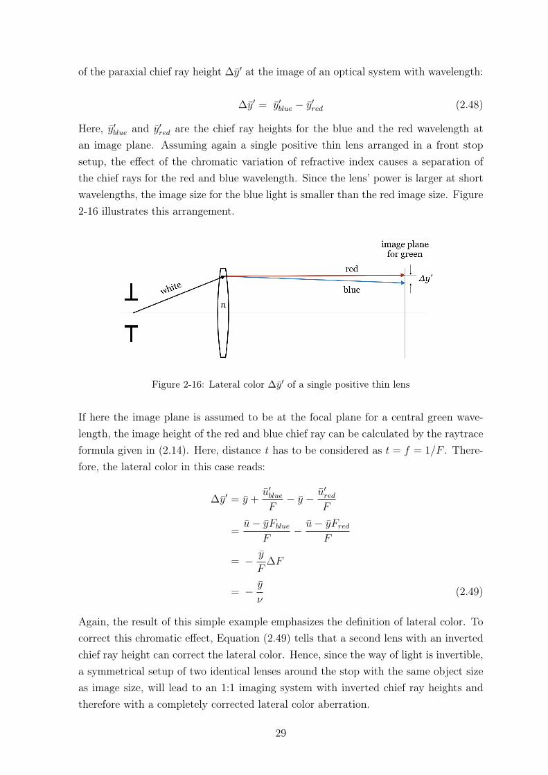
of the paraxial chief ray height ∆𝑦′ at the image of an optical system with wavelength:

∆𝑦′ = 𝑦′𝑏𝑙𝑢𝑒 − 𝑦′𝑟𝑒𝑑 (2.48)

Here, 𝑦′𝑏𝑙𝑢𝑒 and 𝑦′𝑟𝑒𝑑 are the chief ray heights for the blue and the red wavelength atan image plane. Assuming again a single positive thin lens arranged in a front stopsetup, the effect of the chromatic variation of refractive index causes a separation ofthe chief rays for the red and blue wavelength. Since the lens’ power is larger at shortwavelengths, the image size for the blue light is smaller than the red image size. Figure2-16 illustrates this arrangement.

Figure 2-16: Lateral color Δ𝑦′ of a single positive thin lens

If here the image plane is assumed to be at the focal plane for a central green wave-length, the image height of the red and blue chief ray can be calculated by the raytraceformula given in (2.14). Here, distance t has to be considered as 𝑡 = 𝑓 = 1/𝐹 . There-fore, the lateral color in this case reads:

∆𝑦′ = 𝑦 +�̄�′𝑏𝑙𝑢𝑒

𝐹− 𝑦 − �̄�′

𝑟𝑒𝑑

𝐹

=�̄�− 𝑦𝐹𝑏𝑙𝑢𝑒

𝐹− �̄�− 𝑦𝐹𝑟𝑒𝑑

𝐹

= − 𝑦

𝐹∆𝐹

= − 𝑦

𝜈(2.49)

Again, the result of this simple example emphasizes the definition of lateral color. Tocorrect this chromatic effect, Equation (2.49) tells that a second lens with an invertedchief ray height can correct the lateral color. Hence, since the way of light is invertible,a symmetrical setup of two identical lenses around the stop with the same object sizeas image size, will lead to an 1:1 imaging system with inverted chief ray heights andtherefore with a completely corrected lateral color aberration.

29

A surface resolved contribution like the Seidel coefficients again was derived by Welford[Wel86], using a similar approach as for axial color. The result for the system’s sum oflateral color surface contributions is given in Equation (2.50).

𝐶2 =∑︁

𝑛�̄�𝑦

(︂∆𝑛′

𝑛′ − ∆𝑛

𝑛

)︂(2.50)

Here, again ∆𝑛 and ∆𝑛′ describe the dispersion of the optical materials in front of thesurface and behind the surface, respectively. An equivalent thin lens contribution wasobtained by:

𝐶𝐿2 =

∑︁𝑦𝑦∆𝑛𝐿(𝑐1 − 𝑐2) (2.51)

Here, the dispersion of the lens is ∆𝑛𝐿.

2.4 Design Process

During the lens design process, aberration theory and especially the concept of theSeidel coefficients are the main tools to control and to direct the optimization of anoptical system. Considering the given degrees of freedom a lens design contains; likeradii, air spaces, glass selection and stop position, the solution space becomes extremelywide and multi-dimensional [Smi04]. In most of the cases, there are different localminima, meeting a set of optical performance specifications as well as manufacturingand costs constraints. To find the several local solutions, a merit function is set up bythe optical designer. Ensuring the final performance after passing the optical system,typically this merit function is based on ray intersection operands at the final imageplane and on some 1st-order parameters, e.g. focal length, magnification or intersectionlength. An explicit control of certain 3rd-order or even higher-order aberrations isunusual to give meaningful measures of the final image quality. To evaluate the differentsolutions found by the optimizing algorithm, a deeper understanding about how andwhy the lens design works can be achieved by a systematic and continuous analysis ofthe different design states.The best way to find out the inner workings of an optical systems is to understand whythe present left aberrations arise and how they sum up surface by surface to its finalamount at the image plane. This surface or lens resolved analysis is applied by the Sei-del surface or lens contributions. Its main advantage is the identification of performancedominating surfaces or lenses referring to the five primary, 3rd-order aberrations, whichare spherical aberration, coma, astigmatism, field curvature and distortion as well asto the chromatic aberrations. Knowing the single contributions of every lens withinthe optical system enables the designer to work with determined steps like decreasing

30

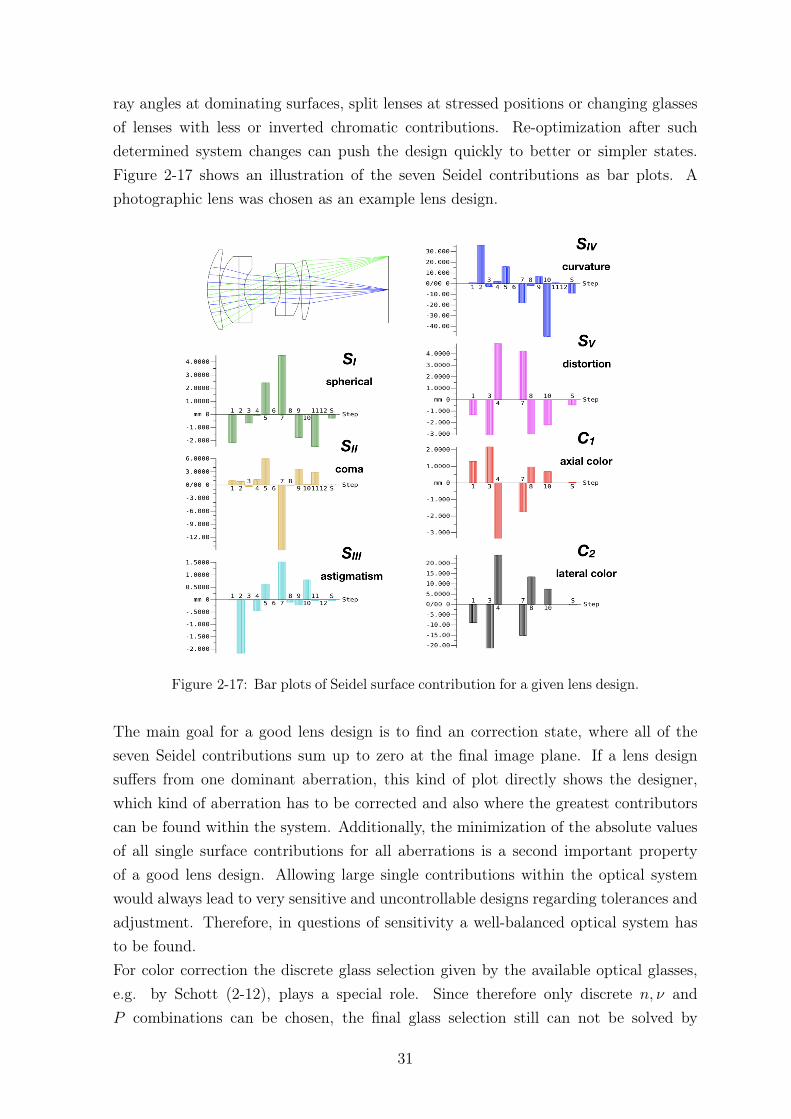
ray angles at dominating surfaces, split lenses at stressed positions or changing glassesof lenses with less or inverted chromatic contributions. Re-optimization after suchdetermined system changes can push the design quickly to better or simpler states.Figure 2-17 shows an illustration of the seven Seidel contributions as bar plots. Aphotographic lens was chosen as an example lens design.

Figure 2-17: Bar plots of Seidel surface contribution for a given lens design.

The main goal for a good lens design is to find an correction state, where all of theseven Seidel contributions sum up to zero at the final image plane. If a lens designsuffers from one dominant aberration, this kind of plot directly shows the designer,which kind of aberration has to be corrected and also where the greatest contributorscan be found within the system. Additionally, the minimization of the absolute valuesof all single surface contributions for all aberrations is a second important propertyof a good lens design. Allowing large single contributions within the optical systemwould always lead to very sensitive and uncontrollable designs regarding tolerances andadjustment. Therefore, in questions of sensitivity a well-balanced optical system hasto be found.For color correction the discrete glass selection given by the available optical glasses,e.g. by Schott (2-12), plays a special role. Since therefore only discrete 𝑛, 𝜈 and𝑃 combinations can be chosen, the final glass selection still can not be solved by

31

a continuously working optimization algorithm, like a damped least squares (DLS)or orthogonal descent (OD) algorithm. Here, an experienced designer is supposedto find the best glass combination by carefully chosen incremental steps inside theAbbe diagram. The main contributors on color aberrations again can be found by theSeidel contributions. But in this case, not only the single surface but the whole lenscontribution has to be considered, since a change of glass always influences the coloreffects of both surfaces of the lens.Although the correction of the five 3rd-order aberrations and the two 1st-order chro-matic aberration is a necessary condition to guarantee a good overall aberration cor-rection, the influence of higher-order aberration can not be neglected in many cases.In contrast to the 3rd-order aberrations, which are completely independent of eachother, 5th-order aberrations are characterized by additional aberration parts that areinduced by prior generated aberrations of lower-order. This special differentiation be-tween induced and intrinsic contributions allows the lens designer not only to analyze,if there are dominating 5th-order aberrations, but it also tells how well the intrinsicand induced parts are balanced. Thereby, large induced aberrations parts refer to ei-ther unbalanced large 3rd-order aberration somewhere inside the system or in somespecial cases large induced contributions even helps to correct the remaining intrinsicparts. This is often used for higher-order color aberrations without direct intention ofthe designer. An analytical tool like the Seidel contributions does not exist so far. Forhigher-order monochromatic aberrations some special design features like asphericalsurfaces can help to correct them, without increasing the amount of elements and thetotal track length. A Seidel equivalent analysis tool for this was found by Buchdahl[Buc54] and Rimmer [Rim63]. 5th-order surface contributions theory in terms of wave-front aberrations was completed by Hoffman [Hof93] and Sasian [Sas10], which alsocan be found in some of today’s lens design software.

2.5 State of the Induced Aberration Problem

The 1st-order theory of the color aberrations and the 3rd-order theory of the monochro-matic aberrations are based on a linearized perturbation theory [Gro+07]. Therefore,a clear surface contribution formula can be derived for all of those aberrations andthe total amount of the system aberrations can be expressed by the sum over all con-tributions. This was shown in Section 2.2.3 and 2.3. However, in realita, ray datadeviates from the paraxial ones during its path in the optical system. The results aresmall, but present differences in ray heights (∆𝑦) and ray angles (∆𝑢) at the refractivesurfaces compared to the paraxial ray data. Induced aberrations are caused by thesedifferences. Therefore, they only occur at higher order aberrations [Ber+15].As today, a multitude of the lens designs are specified to work in broad wavelength

32

ranges, providing large field of views and large apertures within very compact lensdimensions, higher-order aberrations are often the factor that at the end limits theresolution a lens can give [KT02]. Hence, although the correction of the five 3rd-orderaberrations and the two 1st-order chromatic aberrations is a meaningful condition toguarantee a good overall aberration correction, the influence of higher-order aberrationsand therefore also of induced aberrations can not be neglected in most cases.

2.5.1 Induced Monochromatic Aberration

When considering these higher orders of aberrations, the linearity of the 3rd-ordermonochromatic theory is no longer valid and mixing effects of higher perturbation termsoccur. In consequence, at every optical surface, two types of aberration characteristicscan be distinguished [Ber+15]:

1. Intrinsic aberration contributions, that are generated directly at the surface itself.Here it is assumed, that the incoming ray is a paraxial aberration free ray.

2. Induced aberration contributions, which occur, because of the prior summed upaberrations affecting the ray, hitting the surface.

This understanding of monochromatic intrinsic and induced aberration parts is shownin Figure 2-18 for the simple example of a single lens.

Figure 2-18: Monochromatic intrinsic and induced ray aberration parts

Assuming the same ray based approach like Seidel, Buchdahl [Buc54] and Rimmer[Rim63] derived the 5th- and 7th-order surface contributions of the monochromaticaberrations in 1963. Hoffman [Hof93] and Sasian [Sas10] completed 5th-order surfacecontributions theory in terms of wavefront aberration in 1993 and 2010. Clearly, theanalytic expressions for these higher-order surface contributions are no longer as simpleas the originally Seidel surface contributions. However, they are well described today,including the differentiation of intrinsic and induced aberration parts.

33

2.5.2 Induced Axial and Lateral Color

In case of color aberrations, different orders do not refer to their dependency on theray field and pupil coordinates, only. They can also be considered with respect totheir dependency of dispersion. Hence, this approach extends the paraxial theory tosecond and higher-order effects regarding the paraxial ray dependency on dispersion.Thus, the primary axial and lateral color aberration description, introduced in section2.3, linearly depend on the dispersive behavior of the glasses. Nevertheless, in 1987Wynne [Wyn77] [Wyn78] has already shown analytically that for every optical systems,axial color and lateral color are additionally influenced by non-linear contributions, inwhich induced aberrations are part of these nonlinear effects. He found that inducedaberrations can have a significant impact on the correction of secondary axial color andhe identified a way to determine the contribution of induced axial and lateral color bytracing two paraxial rays with different wavelengths. Also in present research today, forsingle selected design examples and certain special cases Roger[Rog13b] [Rog13a] andMcCarthy [Mcc55] obtained analytical expressions for secondary axial color includinginduced aberration parts. Actually, they showed, that there are certain types of op-tical systems that exclusively take advantage of induced aberration effects to obtaina chromatically corrected image. In addition to those special cases, a more generaldescription of the 2nd-order axial color distribution of thin lenses in air was underpresent investigation by Nobis [Nob14] [Nob15]. He derived an axial color contributionincluding higher orders by considering ray based parameters like ray angles, ray heightsand the refractive power of the thin lens. Comparing these different approaches, thereis one particular benefit of Nobis’ descriptive, analytical formula for longitudinal lenscontributions to axial color up to 2nd-order [Nob15]. In contrast to Wynne [Wyn78],his calculation requires ray data of the reference wavelength, only. Hence, a second rayof the other wavelength is not needed to be traced. This was similar to the Seidel sur-face contribution approach for primary color aberration and resulted in the followingequation for the 2nd-order axial color contribution 𝐶𝐻𝐿2𝑛𝑑 of a thin lens in air:

𝐶𝐻𝐿𝐿2𝑛𝑑 =

𝐹

𝑢𝑢′𝐶𝐻𝐿21𝑠𝑡 +

2𝑦∆𝐹

𝑢′ 𝐶𝐻𝐿1𝑠𝑡 +𝑦3∆𝐹 2

𝑢′ (2.52)

Here, a prior 1st-order axial color aberration 𝐶𝐻𝐿1𝑠𝑡, summed up lens by lens in theprevious optical system, was assumed. Reviewing the general definition and differen-tiation of intrinsic and induced aberration parts, described before for monochromaticaberrations, clearly, two terms of induced character are included here. These two termsare the first and second one, since they are depending on the prior summed up 1st-orderaxial color aberration. However, a comparable and equivalent expression for a surfacecontribution on axial and also on lateral color up to 2nd-order is missing literature.

34

2.5.3 Induced Chromatic Variation of 3rd-order Aberrations

Concerning the chromatic variation of 3rd-order aberrations, in particular e.g. for sphe-rochromatism, different orders refer to the dependency of 3rd-order spherical aberrationon 1st-order color aberrations. In this case, there were useful results due to Slyusarev[Sli84], Conrady [Con14] and Hopkins [Hop50]. However, Slyusarev [Sli84] consideredonly the special case of an object at infinity and also didn’t include the 1st-order deriva-tives of the ray based parameters with respect to the refractive index to his approach.Hence, a general expression for spherochromatism was missing here. Furthermore,Conrady [Con14] permits the calculation of all chromatic aberrations, including sphe-rochromatism, by tracing an exact ray at a single wavelength. But, the terms whichwere ignored during his derivation can become significantly high, in case that one partof a lens shows a large amount of color aberration, which is corrected in another widelyseparated part of the lens [KT02]. In other words, induced effects are not consideredwithin Conrady’s approach. Since Hopkin’s solution in [Hop50] is also based on Con-rady’s idea, his results for spherochromatism suffer from the same disadvantages. Toemphasize, in 1986 also Welford [Wel86] already mentioned the simple idea for spec-ifying all of the chromatic variations of aberrations only by differentiating the Seidelcontributions with respect to refractive index. But he also called the expected resultsto be cumbersome and too unwieldy for general use.Hence, in case of the chromatic variation of 3rd-order aberrations, there is a great an-alytical gap concerning Seidel equivalent surface resolved expressions for spherochro-matism, colored coma, colored astigmatism, colored field curvature and for coloreddistortion. Furthermore, following the basic idea of induced aberrations, these missingexpressions are expected to also include induced aberration parts caused by 1st-ordercolor aberrations.

35

3 Extended Induced Color AberrationTheory

3.1 The Concept of Induced Color Aberrations

In analogous manner to the monochromatic aberrations, in general induced aberrationsare higher-order aberrations. They are caused by ray perturbations of lower order,picked up surface by surface in the preceding optical system. This monochromaticconcept can be transferred to the color aberrations.Please note, the following chapter includes a revised version of [BNG17] and [Ber+18],which have been published in advance in 2017 and 2018.

3.1.1 Characteristics

Following the monochromatic approach, induced color aberrations are higher-orderaberrations, caused by small ray perturbations of lower-order color aberrations. Theselower-order color aberrations sum up surface by surface on the light’s way through theoptical system. Therefore, a surface or lens resolved approach is the key method forcharacterizing and understanding them.Regarding a single surface of an optical system, a polychromatic ray trace results insmall ray deviations for the different wavelengths at the investigated surface. Thereason for this is the wavelength depending law of refraction, 𝑛 sin 𝑖 = 𝑛′ sin 𝑖′. Sincethe refractive index n varies with different wavelengths, every refractive surface in frontof the investigated surface leads to small differences in ray angles ∆𝑢 and therefore,after transferring to the next surface, also to small differences in ray heights ∆𝑦. Theraytrace equations (2.12) and (2.14) of Section 2.1.3 illustrates these relations. To thateffect, the prior summed up color aberrations, causing the induced aberration parts,appear as ray perturbations in ray angles and ray heights for the different wavelengthsat the investigates surface of the optical system.Following those considerations, the total amount of a surface contribution on coloraberrations can always be divided into two parts:

36

1. the intrinsic aberration part, which is generated by the dispersion ∆𝑛 of thesurface itself, assuming a perfect, color aberration free incoming ray.

2. the induced aberration part, which is only generated, if a prior color aberratedray hits the surface.

In other words, the intrinsic aberration part ignores all dispersive effects before andthe induced aberration part is only present if a certain separation of the differentwavelengths in ray angles and ray heights occurred before. Please note, all of thesedefinitions are also true for a lens resolved analysis, assuming thin lenses. Hence, Figure3-1 illustrates these considerations by a simple lens design and its differentiation of thetotal axial color aberration into the intrinsic and induced parts.

Figure 3-1: Intrinsic and induced color aberration parts

3.1.2 Aberration Classification

In case of induced color aberrations, the definition of different aberration orders donot refer to the ray dependency on field and pupil coordinates only, this approachextends the aberration theory to higher-order effects regarding the ray dependency ondispersion.

Following this, originating from the paraxial parameters of the intersection length sand the image height y, 1st-order terms result in the well-known Seidel contributions ofaxial color (2.50) and lateral color (2.46) shown in Section 2.3, since they are linearlydepending on dispersion. Consequently, further differentiation with respect to disper-sion then leads to 2nd- or higher-order terms, respectively. In contrast to the 1st-order,these terms also comprise the interaction of linear and higher-order terms. Therefore,dispersive effects between different elements of the optical system are considered. Inconsequence, they include induced color effects by definition, caused by lower 1st-ordercolor aberrations, picked up in the preceding optical system.Increasing as a next step the order of pupil and field dependency, the paraxial region isleft and the primary monochromatic aberrations are obtained. Clearly, these primary

37

monochromatic aberrations as well as all higher-order monochromatic aberrations are ofzero-order in color, since they do not depend on dispersive effects. However, by differen-tiation with respect to the wavelength, the chromatic variations of the monochromaticaberrations are found. They describe the interaction of monochromatic aberrationswith dispersive effects of the optical systems. Therefore, in case of chromatic varyingmonochromatic aberrations, induced aberration terms already occur, if higher-ordermonochromatic aberrations depend on lower-order color aberrations, picked up in thepreceding optical system.

Figure 3-2: Classification of different color aberration orders exemplary shown, startingat (a) paraxial intersection lengths s and (b) image height y. The greenand yellow colored quantities mark the well-known Seidel and Buchdahl co-efficients, respectively. The blue framed quantities include induced coloraberrations.

Figure 3-2 (a) and (b) illustrate exemplary these classifications, starting at the paraxialparameters of the intersection lengths s and the image height y. The monochromaticaberration denotations are based on Seidel’s [KT02] and Buchdahl’s definitions [Buc54].The prefix "c" indicates the chromatic variation of the individual quantity. Please note,all of the blue framed quantities consist of an intrinsic as well as an induced aberrationpart.

3.1.3 Overview of new Results in this Chapter

The Sections 2.5.2 and 2.5.3 already gave information about the current state of theinduced color aberration problem. There were noteworthy contributions by Nobis

38

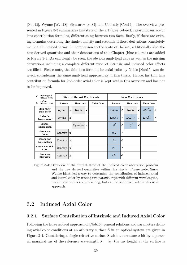
[Nob15], Wynne [Wyn78], Slyusarev [Sli84] and Conrady [Con14]. The overview pre-sented in Figure 3-3 summarizes this state of the art (grey colored) regarding surface orlens contribution formulas, differentiating between two facts, firstly, if there are exist-ing formulas describing the single quantity and secondly if those derivations completelyinclude all induced terms. In comparison to the state of the art, additionally also thenew derived quantities and their denotations of this Chapter (blue colored) are addedto Figure 3-3. As can clearly be seen, the obvious analytical gaps as well as the missingderivations including a complete differentiation of intrinsic and induced color effectsare filled. Please note, the thin lens formula for axial color by Nobis [Nob15] was de-rived, considering the same analytical approach as in this thesis. Hence, his thin lenscontribution formula for 2nd-order axial color is kept within this overview and has notto be improved.

Figure 3-3: Overview of the current state of the induced color aberration problemand the new derived quantities within this thesis. Please note, SinceWynne identified a way to determine the contribution of induced axialand lateral color by tracing two paraxial rays with different wavelengths,his induced terms are not wrong, but can be simplified within this newapproach.

3.2 Induced Axial Color

3.2.1 Surface Contribution of Intrinsic and Induced Axial Color

Following the lens-resolved approach of [Nob15], general relations and parameters defin-ing axial color conditions at an arbitrary surface S in an optical system are given inFigure 3-4. Considering a single refractive surface S with a curvature c hit by a parax-ial marginal ray of the reference wavelength 𝜆 = 𝜆1, the ray height at the surface is

39

y, the ray angle before the surface is u, and the ray angle after the surface is 𝑢′. Thematerials before and after the surface are characterized by their individual refractiveindices n and 𝑛′ , respectively.

Figure 3-4: Refraction of two paraxial marginal rays with different wavelengths(black and blue line) at an arbitrary surface S

The intersection length s between the refractive surface and the intermediate imagebefore, which is assumed to lie on a finite distance, is the result of

𝑠(𝑦, 𝑢) = −𝑦

𝑢(3.1)

To define the intersection lengths 𝑠′ after refraction, the definition for the refractivepower F of a single surface (2.9) and the paraxial ray trace formula (2.12) have to beconsidered. Consequently, the intersection lengths s’ after refraction results in:

𝑠′(𝑦, 𝑢, 𝑛, 𝑛′) = − 𝑦

𝑢′

= − 𝑦𝑛′

𝑛𝑢− 𝑦(𝑛′ − 𝑛)𝑐(3.2)

Considering a second wavelength 𝜆2 = 𝜆1 + ∆𝜆, the corresponding ray height 𝑦2 at thesurface is 𝑦2 = 𝑦 + ∆𝑦 and the ray angles before and after the surface are 𝑢2 = 𝑢+ ∆𝑢

and 𝑢′2 = 𝑢′ + ∆𝑢′. Similarly, the refractive indices show a wavelength dependent,

dispersive behavior with 𝑛2 = 𝑛+∆𝑛 and 𝑛′2 = 𝑛′ +∆𝑛′. Reviewing now the definition

in Section 2.3.1, axial color can be described as the change of intersection length of anoptical system with wavelength. Hence, the axial color aberrations before and after

40

the surface, ∆𝑠 and ∆𝑠′, within a wavelength range from𝜆1 to 𝜆2 are given by

∆𝑠 = 𝑠𝜆2 − 𝑠

= 𝑠(𝑦 + ∆𝑦, 𝑢 + ∆𝑢) − 𝑠(𝑦, 𝑢) (3.3)

∆𝑠′ = 𝑠′𝜆2 − 𝑠′

= 𝑠′(𝑦 + ∆𝑦, 𝑢 + ∆𝑢, 𝑛 + ∆𝑛, 𝑛′ + ∆𝑛′) − 𝑠′(𝑦, 𝑢, 𝑛, 𝑛′) (3.4)

If the differences ∆𝑦,∆𝑢,∆𝑛 and ∆𝑛′ are small, a Taylor series expansion can be ap-plied. Since all of these differences occurred because of dispersion within the opticalsystem, an expansion up to second order refer to the 2nd-order color aberration clas-sification of Section 3.1.2. Hence, the following expressions for the intersection lengths𝑠𝜆2 and 𝑠′𝜆2 are obtained:

𝑠𝜆2 = 𝑠(𝑦, 𝑢) +𝜕𝑠

𝜕𝑦∆𝑦 +

𝜕𝑠

𝜕𝑢∆𝑢 +

1

2

𝜕2𝑠

𝜕𝑦2∆𝑦2 +

𝜕2𝑠

𝜕𝑦𝜕𝑢∆𝑦∆𝑢 +

1

2

𝜕2𝑠

𝜕𝑢2∆𝑢2 (3.5)

𝑠′𝜆2 = 𝑠′(𝑦, 𝑢, 𝑛, 𝑛′) +𝜕𝑠′

𝜕𝑦∆𝑦 +

𝜕𝑠′

𝜕𝑢∆𝑢 +

𝜕𝑠′

𝜕𝑛∆𝑛 +

𝜕𝑠′

𝜕𝑛′∆𝑛′

+1

2

𝜕2𝑠′

𝜕𝑦2∆𝑦2 +

𝜕2𝑠′

𝜕𝑦𝜕𝑢∆𝑦∆𝑢 +

𝜕2𝑠′

𝜕𝑦𝜕𝑛∆𝑦∆𝑛 +

𝜕2𝑠′

𝜕𝑦𝜕𝑛′∆𝑦∆𝑛′

+1

2

𝜕2𝑠′

𝜕𝑢2∆𝑢2 +

𝜕2𝑠′

𝜕𝑢𝜕𝑛∆𝑢∆𝑛 +

𝜕2𝑠′

𝜕𝑢𝜕𝑛′∆𝑢∆𝑛′ +1

2

𝜕2𝑠′

𝜕𝑛2∆𝑛2

+𝜕2𝑠′

𝜕𝑛𝜕𝑛′∆𝑛∆𝑛′ +1

2

𝜕2𝑠′

𝜕𝑛′2∆𝑛′2 (3.6)

Inserting this into Equation (3.3) and (3.4), the axial color before and after the refrac-tive surface results in:

∆𝑠 =𝜕𝑠

𝜕𝑦∆𝑦 +

𝜕𝑠

𝜕𝑢∆𝑢 +

1

2

𝜕2𝑠

𝜕𝑦2∆𝑦2 +

𝜕2𝑠

𝜕𝑦𝜕𝑢∆𝑦∆𝑢 +

1

2

𝜕2𝑠

𝜕𝑢2∆𝑢2 (3.7)

∆𝑠′ =𝜕𝑠′

𝜕𝑦∆𝑦 +

𝜕𝑠′

𝜕𝑢∆𝑢 +

𝜕𝑠′

𝜕𝑛∆𝑛 +

𝜕𝑠′

𝜕𝑛′∆𝑛′

+1

2

𝜕2𝑠′

𝜕𝑦2∆𝑦2 +

𝜕2𝑠′

𝜕𝑦𝜕𝑢∆𝑦∆𝑢 +

𝜕2𝑠′

𝜕𝑦𝜕𝑛∆𝑦∆𝑛 +

𝜕2𝑠′

𝜕𝑦𝜕𝑛′∆𝑦∆𝑛′

+1

2

𝜕2𝑠′

𝜕𝑢2∆𝑢2 +

𝜕2𝑠′

𝜕𝑢𝜕𝑛∆𝑢∆𝑛 +

𝜕2𝑠′

𝜕𝑢𝜕𝑛′∆𝑢∆𝑛′ +1

2

𝜕2𝑠′

𝜕𝑛2∆𝑛2

+𝜕2𝑠′

𝜕𝑛𝜕𝑛′∆𝑛∆𝑛′ +1

2

𝜕2𝑠′

𝜕𝑛′2∆𝑛′2 (3.8)

41

1st-order terms At first only the derivatives of the linear terms, e.g. the 1st-orderterms, are considered. When inserting the derivatives for ∆𝑠 and ∆𝑠′, attached inAppendix, the following equations are obtained:

∆𝑠1𝑠𝑡 = − 1

𝑢∆𝑦 +

𝑦

𝑢2∆𝑢 (3.9)

∆𝑠′1𝑠𝑡 = − 𝑛𝑢

𝑛′𝑢′2∆𝑦 +𝑛𝑦

𝑛′𝑢′2∆𝑢 +𝑦𝑖

𝑛′𝑢′2∆𝑛− 𝑛𝑦𝑖

𝑛′2𝑢′2∆𝑛′ (3.10)

Here, i is the paraxial incident angle of the marginal ray with 𝑖 = 𝑢 + 𝑦𝑐 (see Section2.1.2). To specify the axial color contribution 𝐴𝑋𝐶𝑆

1𝑠𝑡 of the refractive surface, thedifference of the axial color aberration at the intermediate image after the surface ∆𝑠′1𝑠𝑡

and the axial color aberration at the intermediate image in front of the surface ∆𝑠1𝑠𝑡

has to be considered. Since these axial color aberrations are longitudinal aberrationsat a specific intermediate image, the axial magnification 𝛼 = 𝑛𝑢2/𝑛′𝑢′2 between theconsidered intermediate image and the final image needs to be taken into account asa longitudinal scaling factor (see Section 2.4). Note that, in the case of intermediateimages of surfaces, the axial magnification not only depends on the marginal ray anglesbut also on the refractive indices of the individual materials.Following these considerations, the 1st-order axial color surface contribution 𝐴𝑋𝐶𝑆

1𝑠𝑡

is given by

𝐴𝑋𝐶𝑆1𝑠𝑡 = ∆𝑠′1𝑠𝑡(−𝑛′𝑢′2) − ∆𝑠1𝑠𝑡(−𝑛𝑢2) (3.11)

Inserting and simplifying Equation (3.9) and (3.10) leads to the following relation:

𝐴𝑋𝐶𝑆1𝑠𝑡 =

(︂− 𝑛𝑢

𝑛′𝑢′2∆𝑦 +𝑛𝑦

𝑛′𝑢′2∆𝑢 +𝑦𝑖

𝑛′𝑢′2∆𝑛− 𝑛𝑦𝑖

𝑛′2𝑢′2∆𝑛′)︂

(−𝑛′𝑢′2)

−(︂− 1

𝑢∆𝑦 +

𝑦

𝑢2∆𝑢

)︂(−𝑛𝑢2) (3.12)

𝐴𝑋𝐶𝑆1𝑠𝑡 = 𝑛𝑖𝑦

(︂∆𝑛′

𝑛′ − ∆𝑛

𝑛

)︂(3.13)

This result agrees with the common Seidel theory of primary axial color, shown inSection 2.3.1.

2nd-order terms In analogous manner to the 1st-order terms, the nonlinear termsare obtained. Consequently, the 2nd-order axial color effects of an arbitrary surfaceequals to:

𝐴𝑋𝐶𝑆2𝑛𝑑 = ∆𝑠′2𝑛𝑑(−𝑛′𝑢′2) − ∆𝑠2𝑛𝑑(−𝑛𝑢2) (3.14)

42

Here, the following relations for the 2nd-order terms ∆𝑠2𝑛𝑑 and ∆𝑠′2𝑛𝑑 are applied.

∆𝑠2𝑛𝑑 =1

2

𝜕2𝑠

𝜕𝑦2∆𝑦2 +

𝜕2𝑠

𝜕𝑦𝜕𝑢∆𝑦∆𝑢 +

1

2

𝜕2𝑠

𝜕𝑢2∆𝑢2 (3.15)

∆𝑠′2𝑛𝑑 =1

2

𝜕2𝑠′

𝜕𝑦2∆𝑦2 +

𝜕2𝑠′

𝜕𝑦𝜕𝑢∆𝑦∆𝑢 +

𝜕2𝑠′

𝜕𝑦𝜕𝑛∆𝑦∆𝑛 +

𝜕2𝑠′

𝜕𝑦𝜕𝑛′∆𝑦∆𝑛′

+1

2

𝜕2𝑠′

𝜕𝑢2∆𝑢2 +

𝜕2𝑠′

𝜕𝑢𝜕𝑛∆𝑢∆𝑛 +

𝜕2𝑠′

𝜕𝑢𝜕𝑛′∆𝑢∆𝑛′ +1

2

𝜕2𝑠′

𝜕𝑛2∆𝑛2

+𝜕2𝑠′

𝜕𝑛𝜕𝑛′∆𝑛∆𝑛′ +1

2

𝜕2𝑠′

𝜕𝑛′2∆𝑛′2 (3.16)

Inserting the 2nd-order derivatives, attached at the appendix, a slightly more complexexpression compared to the thin lens approach of [Nob14] is achieved. This is causedby the additional terms depending on ∆𝑛 and ∆𝑛′. Following the idea of inducedaberrations, illustrated in Section 3.1, some of the 2nd-order terms have to dependon the cumulative preexisting lower-order aberrations in the system before. Hence, inthe case of a single refractive surface, there have to be some of the 2nd-order terms,depending on the 1st-order axial color aberration in front of the surface, which wasalready described by Equation (3.9). Multiplied by the magnification factor, Equation(3.17) shows the expression 𝐴𝑋𝐶1𝑠𝑡 characterizing the preexisting 1st-order axial coloraberration in front of the surface.

𝐴𝑋𝐶1𝑠𝑡 = ∆𝑠1𝑠𝑡(−𝑛𝑢2) = 𝑛𝑢∆𝑦 − 𝑛𝑦∆𝑢 (3.17)

Analyzing now the 2nd-order terms for a dependence on this expression, the 2nd-orderaxial color surface contribution is obtained after simplifying with common relations forray tracing (Section 2.1.3):

𝐴𝑋𝐶𝑆2𝑛𝑑 =

𝐹

𝑛𝑛′𝑢𝑢′𝐴𝑋𝐶21𝑠𝑡 +

𝑢′ + 2𝑦𝑐

𝑢′

(︂∆𝑛′

𝑛′ − ∆𝑛

𝑛

)︂𝐴𝑋𝐶1𝑠𝑡 +

𝑛2𝑖2𝑦

𝑛′𝑢′

(︂∆𝑛′

𝑛′ − ∆𝑛

𝑛

)︂2

− 𝑛𝑖𝑦

(︂∆𝑛′2

𝑛′2 − ∆𝑛′∆𝑛

𝑛′𝑛

)︂(3.18)

This equation is one of the main results of this thesis.

3.2.2 Lens Contribution of Intrinsic and Induced Axial Color

Since induced aberrations are caused by the small differences in ray heights and rayangles due to the prior lower-order aberrations, especially the influence of the distancebetween two lens surfaces will be of greater interest. Furthermore, a derivation of a

43

2nd-order axial color thick lens contribution will be more instructive for an opticaldesigner than a surface resolved contribution, as color correction is usually connectedto changing glasses of lenses, not surfaces.

Figure 3-5: Refraction of the marginal ray at a thick lens. The marginal ray heightsand angles are 𝑦1 and 𝑢1 as well as 𝑦2 and 𝑢2 at surface S1 and surfaceS2, respectively.

To find an analytical description for a lens in air with a thickness t and a refractive indexof n, Equation (3.18) can be considered for the two surfaces of a thick lens applying aparaxial ray trace for the ray propagation within this lens. Figure 3-5 illustrates therelevant quantities for the thick lens approach. The preexisting 1st-order axial colorfor surface S1 is again 𝐴𝑋𝐶1𝑠𝑡 and according to the Seidel surface coefficient for axialcolor 𝐶1 (Section 2.3.1, Equation (2.46)) shows the preexisting axial color for surfaceS2 is:

𝐴𝑋𝐶 ′1𝑠𝑡 = 𝐴𝑋𝐶1𝑠𝑡 + 𝑦1𝑖1

∆𝑛

𝑛(3.19)

Considering now a certain thickness t for an individual lens in an optical system the2nd-order axial color thick lens contribution 𝐴𝑋𝐶𝑡𝐿

2𝑛𝑑 can be calculated by the sum ofboth surface contributions.

𝐴𝑋𝐶 𝑡𝐿2𝑛𝑑 = 𝐴𝑋𝐶𝑆1

2𝑛𝑑 + 𝐴𝑋𝐶𝑆22𝑛𝑑 (3.20)

with a surface contribution 𝐴𝑋𝐶𝑆12𝑛𝑑 of surface S1:

𝐴𝑋𝐶𝑆12𝑛𝑑 =

𝐹1

𝑛𝑢0𝑢1

𝐴𝑋𝐶21𝑠𝑡 +

𝑢1 + 2𝑦1𝑐1𝑢1

∆𝑛

𝑛𝐴𝑋𝐶1𝑠𝑡 +

𝑖21𝑦1𝑛𝑢1

(︂∆𝑛

𝑛

)︂2

− 𝑖1𝑦1

(︂∆𝑛2

𝑛2

)︂(3.21)

44

and a second surface contribution 𝐴𝑋𝐶𝑆22𝑛𝑑 of surface S2:

𝐴𝑋𝐶𝑆22𝑛𝑑 =

𝐹2

𝑛𝑢1𝑢2

𝐴𝑋𝐶 ′21𝑠𝑡 −

𝑢2 + 2𝑦2𝑐2𝑢2

∆𝑛

𝑛𝐴𝑋𝐶 ′

1𝑠𝑡 +𝑛2𝑖22𝑦2𝑛𝑢2

(︂∆𝑛

𝑛

)︂2

(3.22)

The indices 0, 1 and 2 are used for ray data according to Figure 3-5. Here, the lens’thickness t is represented in Equation (3.22) by the raytrace parameters 𝑦2(𝑡), 𝑖2(𝑦2) and𝑢2(𝑦2). Inserting now Equations (3.21) and (3.22) into Equation (3.20) and rearrangingas well as simplifying the terms, the following thick lens formula is achieved:

𝐴𝑋𝐶 𝑡𝐿2𝑛𝑑 =

𝐹𝐿

𝑢0𝑢2

𝐴𝑋𝐶21𝑠𝑡 +

2𝑦1(𝑐1 − 𝑐2)∆𝑛

𝑢2

𝐴𝑋𝐶1𝑠𝑡 +𝑦31(𝑐1 − 𝑐2)

2

𝑢2

∆𝑛

+ 𝑡(𝑛− 1)𝑐1𝑐2

𝑛𝑢0𝑢2

𝐴𝑋𝐶21𝑠𝑡 − 𝑡

𝛼1∆𝑛

𝑛𝑢2

𝐴𝑋𝐶1𝑠𝑡 + 𝑡𝛼2

𝑛𝑢2

∆𝑛2 (3.23)

The coefficients 𝛼1 and 𝛼2(𝑡) can be found in the appendix. Comparing this withNobis’ thin lens formula (2.52) shown in Section 2.5.2 and considering the relation∆𝐹𝐿 = ∆𝑛(𝑐1 − 𝑐2), a consistent relation to his results is obtained.

𝐴𝑋𝐶 𝑡𝐿2𝑛𝑑 = 𝐶𝐻𝐿 𝐿

2𝑛𝑑 + 𝑡(𝑛− 1)𝑐1𝑐2

𝑛𝑢0𝑢2

𝐴𝑋𝐶21𝑠𝑡 − 𝑡

𝑎1∆𝑛

𝑛𝑢2

𝐴𝑋𝐶1𝑠𝑡 + 𝑡𝑎2(𝑡)

𝑛𝑢2

∆𝑛2 (3.24)

3.2.3 Discussion

A Taylor expansion of the surface resolved axial color considering derivatives up to2nd-order results in Equation (3.18).

Induced and Intrinsic Terms There are four terms. The first two terms dependon the preexisting 1st-order axial color aberration in front of the surface. Hence, theyare of induced character, since they vanish, if there is no preexisting axial color. Thelast two terms are pure dispersion depending terms. They show only dependencies onthe chromatic variation of the refractive indices before and after the surface ∆𝑛 and∆𝑛′ without any additional dispersion-depending quantities. Hence, these terms areintrinsic terms of 2nd-order.In detail, the first 2nd- order term 𝐹

𝑛𝑛′𝑢𝑢′𝐴𝑋𝐶21𝑠𝑡 shows a quadratic dependence on the

preexisting cumulative 1st-order axial color 𝐴𝑋𝐶1𝑠𝑡 without any additional wavelengthdepending quantities. Hence, this term describes an induced 2nd-order contributionof an optical surface, which is not required to be made of a dispersive material. Forthat case, even a mirror with a specific refractive power F can show this induced axialcolor 2nd-order effect, if a relevant amount of prior summed up axial color aberration

45

is present.The second term 𝑢′+2𝑦𝑐

𝑢′

(︀Δ𝑛′

𝑛′ − Δ𝑛𝑛

)︀𝐴𝑋𝐶1𝑠𝑡 of Equation (3.18) is characterized by its

linear dependency on the preexisting axial color. This term is also an induced one,as it describes the interaction between the summed up 1st-order axial color with adispersive refracting surface. For a mirror, this contribution vanishes.In contrast to the first two terms, the third term 𝑛2𝑖2𝑦

𝑛′𝑢′

(︀Δ𝑛′

𝑛′ − Δ𝑛𝑛

)︀2 is of intrinsic char-acter, as it is caused by pure dispersive effects only. Hence, if there is no preexistingaxial color, this 2nd-order term will still be non- zero, unless the surface is positionedat an intermediate image, where y equals to zero or in the case of normal incidence.The character of the fourth term 𝑛𝑖𝑦

(︀Δ𝑛′2

𝑛′2 − Δ𝑛′Δ𝑛𝑛′𝑛

)︀is similar to the third one. All of

the considerations for the third term are also true for this last one. Additionally, itshows a dependence on the individual surface type. If it is a back surface in air, thisterm vanishes as ∆𝑛′ for air is zero. But for a cemented surface or front surface in air,the fourth term introduces a certain 2nd -order contribution to axial color.

Required Parameters Beneficial, due to the Seidel sum definition (2.46), the 1st-order axial color 𝐴𝑋𝐶1𝑠𝑡 before an individual surface 𝑆𝑗 inside an optical system caneasily be calculated by summing up all of the 1st-order surface contributions up tosurface 𝑗 − 1 by:

𝐴𝑋𝐶1𝑠𝑡 =

𝑗−1∑︁𝑎=1

𝐴𝑋𝐶𝑆1𝑠𝑡

=

𝑗−1∑︁𝑎=1

𝑛𝑎𝑖𝑎𝑦𝑎

(︂∆𝑛′

𝑛′ − ∆𝑛

𝑛

)︂𝑎

(3.25)

Therefore, all terms in Equation (3.18) are determined by paraxial marginal ray datafor the reference wavelength, only. Hence, one paraxial raytrace for the referencewavelength provides all required parameters for calculating the 2nd-order axial coloreffects. An additional raytrace for another wavelength is not necessary.

Lens Contribution Note that the results and the discussion of the first three 2nd-order surface contribution terms is very similar to the outcome of Nobis’ thin lensresolved analysis for axial color [Nob14]. Comparing both results, the most noticeablefact is the additional intrinsic term in the new surface resolved description. But bycompleting the new surface contribution with its deduced thick lens contribution, de-rived in Equation (3.23), the derivation shows that for lenses the additional intrinsicterm of 2nd-order cancels out. Therefore, the new surface based approach is completelyconsistent and describes a consequent enhancement of Nobis’ approach. Consequently,the thick lens formula consists of four sums, the thin lens contribution and three thick-

46

ness depending terms. The latter one can again be divided in thickness dependinginduced terms 𝑡 (𝑛−1)𝑐1𝑐2

𝑛𝑢0𝑢2𝐴𝑋𝐶2

1𝑠𝑡 and 𝑡𝑎1Δ𝑛𝑛𝑢2

𝐴𝑋𝐶1𝑠𝑡, as well as one thickness dependingintrinsic term 𝑡𝑎2(𝑡)

𝑛𝑢2∆𝑛2. According to the coefficient 𝑎2(𝑡), given in the appendix, the

intrinsic term includes linear as well as quadratic and cubic dependencies on t.

3.3 Induced Lateral Color

3.3.1 Surface Contribution of Intrinsic and Induced Lateral

Color

In this section an equivalent approach for lateral color is introduced. Figure 3-6 il-lustrates the parameters and relations defining lateral color conditions at an arbitrarysurface S in an optical system.

Figure 3-6: Refraction of two paraxial chief rays with different wavelengths (blackand blue line) at an arbitrary surface S. The intermediate images showdifferent lateral color aberrations Δ𝑦1 and Δ𝑦′1 , whereby the imageposition is defined by the intersection length of the marginal ray (dashedline)

Considering a single refractive surface S with a curvature c hit by a paraxial chief andmarginal ray of the reference wavelength 𝜆 = 𝜆1, the chief ray height at the surface is 𝑦and the marginal ray height is y. The chief and marginal ray angles before the surfaceare �̄� and u, respectively, and the chief and marginal ray angles after the surface are�̄�′ and u’, respectively. At the intermediate images in front and after the surface, thechief ray heights are 𝑦1 and 𝑦′1. Since the position of these intermediate images arefixed by the marginal ray’s intersection lengths s and s’, 𝑦1 and 𝑦′1 can be obtained by

𝑦1(𝑦, �̄�) = 𝑦 + 𝑠�̄� (3.26)

𝑦′1(𝑦, �̄�′) = 𝑦 + 𝑠′�̄�′ (3.27)

47

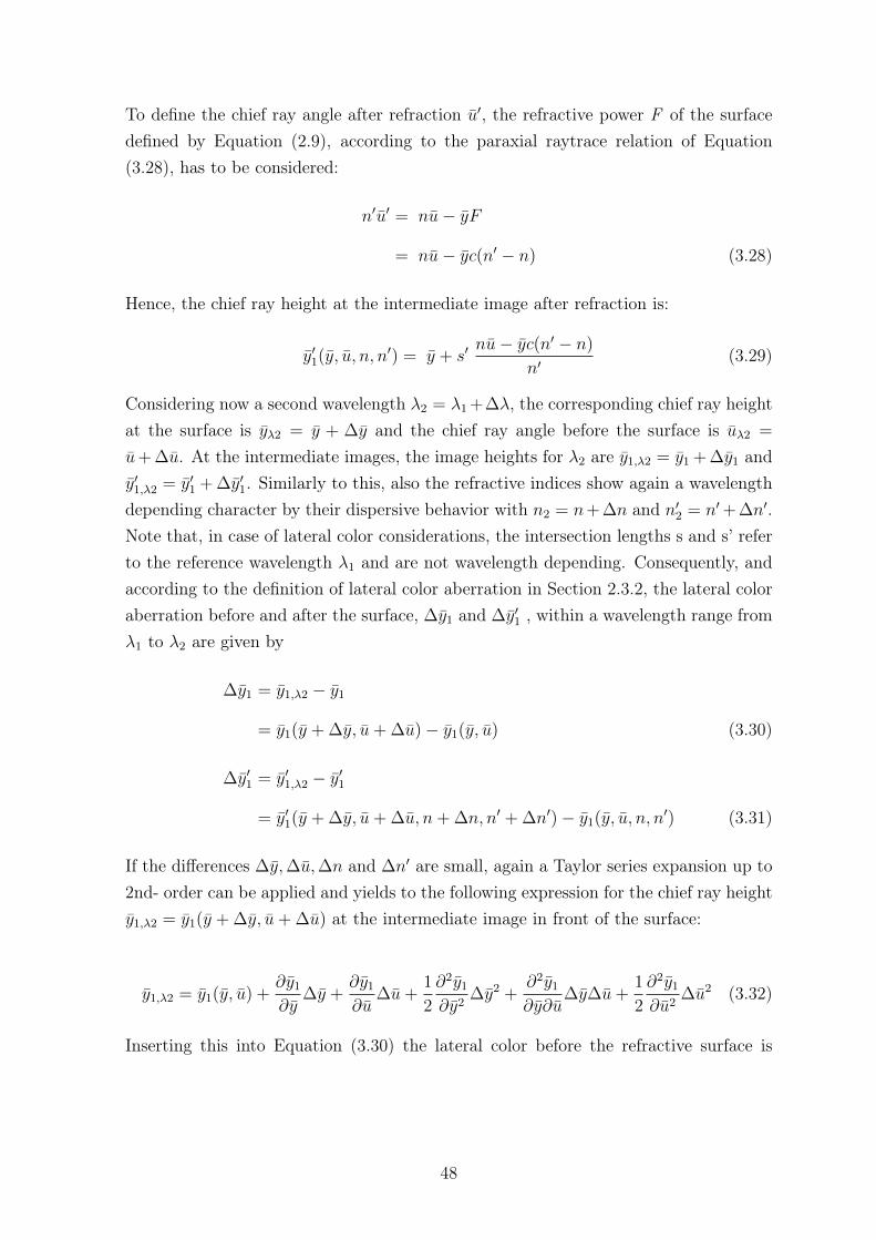
To define the chief ray angle after refraction �̄�′, the refractive power F of the surfacedefined by Equation (2.9), according to the paraxial raytrace relation of Equation(3.28), has to be considered:

𝑛′�̄�′ = 𝑛�̄�− 𝑦𝐹

= 𝑛�̄�− 𝑦𝑐(𝑛′ − 𝑛) (3.28)

Hence, the chief ray height at the intermediate image after refraction is:

𝑦′1(𝑦, �̄�, 𝑛, 𝑛′) = 𝑦 + 𝑠′

𝑛�̄�− 𝑦𝑐(𝑛′ − 𝑛)

𝑛′ (3.29)

Considering now a second wavelength 𝜆2 = 𝜆1 +∆𝜆, the corresponding chief ray heightat the surface is 𝑦𝜆2 = 𝑦 + ∆𝑦 and the chief ray angle before the surface is �̄�𝜆2 =

�̄�+ ∆�̄�. At the intermediate images, the image heights for 𝜆2 are 𝑦1,𝜆2 = 𝑦1 + ∆𝑦1 and𝑦′1,𝜆2 = 𝑦′1 + ∆𝑦′1. Similarly to this, also the refractive indices show again a wavelengthdepending character by their dispersive behavior with 𝑛2 = 𝑛+ ∆𝑛 and 𝑛′

2 = 𝑛′ + ∆𝑛′.Note that, in case of lateral color considerations, the intersection lengths s and s’ referto the reference wavelength 𝜆1 and are not wavelength depending. Consequently, andaccording to the definition of lateral color aberration in Section 2.3.2, the lateral coloraberration before and after the surface, ∆𝑦1 and ∆𝑦′1 , within a wavelength range from𝜆1 to 𝜆2 are given by

∆𝑦1 = 𝑦1,𝜆2 − 𝑦1

= 𝑦1(𝑦 + ∆𝑦, �̄� + ∆�̄�) − 𝑦1(𝑦, �̄�) (3.30)

∆𝑦′1 = 𝑦′1,𝜆2 − 𝑦′1

= 𝑦′1(𝑦 + ∆𝑦, �̄� + ∆�̄�, 𝑛 + ∆𝑛, 𝑛′ + ∆𝑛′) − 𝑦1(𝑦, �̄�, 𝑛, 𝑛′) (3.31)

If the differences ∆𝑦,∆�̄�,∆𝑛 and ∆𝑛′ are small, again a Taylor series expansion up to2nd- order can be applied and yields to the following expression for the chief ray height𝑦1,𝜆2 = 𝑦1(𝑦 + ∆𝑦, �̄� + ∆�̄�) at the intermediate image in front of the surface:

𝑦1,𝜆2 = 𝑦1(𝑦, �̄�) +𝜕𝑦1𝜕𝑦

∆𝑦 +𝜕𝑦1𝜕�̄�

∆�̄� +1

2

𝜕2𝑦1𝜕𝑦2

∆𝑦2 +𝜕2𝑦1𝜕𝑦𝜕�̄�

∆𝑦∆�̄� +1

2

𝜕2𝑦1𝜕�̄�2

∆�̄�2 (3.32)

Inserting this into Equation (3.30) the lateral color before the refractive surface is

48

obtained by:

∆𝑦1 =𝜕𝑦1𝜕𝑦

∆𝑦 +𝜕𝑦1𝜕�̄�

∆�̄� +1

2

𝜕2𝑦1𝜕𝑦2

∆𝑦2 +𝜕2𝑦1𝜕𝑦𝜕�̄�

∆𝑦∆�̄� +1

2

𝜕2𝑦1𝜕�̄�2

∆�̄�2 (3.33)

Applying the same for 𝑦′1 and ∆𝑦′1 leads to the following result:

∆𝑦′1 =𝜕𝑦′1𝜕𝑦

∆𝑦 +𝜕𝑦′1𝜕�̄�

∆�̄� +𝜕𝑦′1𝜕𝑛

∆𝑛 +𝜕𝑦′1𝜕𝑛′ ∆𝑛′

+1

2

𝜕2𝑦′1𝜕𝑦2

∆𝑦2 +𝜕2𝑦′1𝜕𝑦𝜕�̄�

∆𝑦∆�̄� +𝜕2𝑦′1𝜕𝑦𝜕𝑛

∆𝑦∆𝑛 +𝜕2𝑦′1𝜕𝑦𝜕𝑛′∆𝑦∆𝑛′

+1

2

𝜕2𝑦′1𝜕�̄�2

∆�̄�2 +𝜕2𝑦′1𝜕�̄�𝜕𝑛

∆�̄�∆𝑛 +𝜕2𝑦′1𝜕�̄�𝜕𝑛′∆�̄�∆𝑛′

+1

2

𝜕2𝑦′1𝜕𝑛2

∆𝑛2 +𝜕2𝑦′1𝜕𝑛𝜕𝑛′∆𝑛∆𝑛′

+1

2

𝜕2𝑦′1𝜕𝑛′2 ∆𝑛′2 (3.34)

1st-order terms At first again only the derivatives of the 1st-order terms, e.g. thelinear terms, are considered. When inserting the derivatives for ∆𝑦1 and ∆𝑦′1, given atthe appendix, the following equations are obtained:

∆𝑦1,1𝑠𝑡 = ∆𝑦 + 𝑠∆�̄� = ∆𝑦 − 𝑦

𝑢∆�̄� (3.35)

∆𝑦′1,1𝑠𝑡 = ∆𝑦 − 𝑠′𝑐(𝑛′ − 𝑛)

𝑛′ ∆𝑦 +𝑠′𝑛

𝑛′ ∆�̄� +𝑠′̄𝑖

𝑛′ ∆𝑛− 𝑛𝑠′̄𝑖

𝑛′2 ∆𝑛′ (3.36)

Here, i is the incident angle of the chief ray with �̄� = �̄�+𝑦𝑐. To describe now the lateralcolor surface contribution 𝐿𝐴𝐶𝑆

1𝑠𝑡 of the refractive surface, the difference between thelateral color aberration ∆𝑦′1,1𝑠𝑡 at the intermediate image after the surface and thelateral color aberration ∆𝑦1,1𝑠𝑡 at the intermediate image in front of the surface hasto be considered. Since these lateral color aberrations are determined as transverseaberrations at a specific intermediate image, the magnification 𝛽 = (𝑛𝑢)/(𝑛′𝑢′) betweenthe considered intermediate image and the final image needs to be taken into accountas a scaling factor (Section 2.4). Note again, in the case of intermediate images ofsurfaces, the magnification not only depends on the marginal ray angles but also onthe refractive indices of the individual materials. Following these considerations, the1st-order lateral color surface contribution 𝐿𝐴𝐶𝑆

1𝑠𝑡 is equal to:

𝐿𝐴𝐶𝑆1𝑠𝑡 = ∆𝑦′1,1𝑠𝑡(𝑛

′𝑢′) − ∆𝑦1,1𝑠𝑡(𝑛𝑢) (3.37)

49

Now, inserting Equation (3.35) and (3.36) leads to the following relation:

𝐿𝐴𝐶𝑆1𝑠𝑡 = 𝑛′𝑢′∆𝑦 − 𝑢′𝑠′𝑐(𝑛′ − 𝑛)∆𝑦 + 𝑛𝑢′𝑠′∆�̄� + 𝑢′𝑠′̄𝑖∆𝑛− 𝑢′𝑛𝑠

′̄𝑖

𝑛′ ∆𝑛′

− 𝑛𝑢∆𝑦 − 𝑛𝑢𝑠∆�̄� (3.38)

Considering now Equation (3.1) and (3.2) for the intersection lengths s and s’ of themarginal ray, the 1st-order lateral color surface contribution 𝐿𝐴𝐶𝑆

1𝑠𝑡 is given by:

𝐿𝐴𝐶𝑆1𝑠𝑡 = 𝑛�̄�𝑦

(︂∆𝑛′

𝑛′ − ∆𝑛

𝑛

)︂(3.39)

This result agrees with the common Seidel theory of primary lateral color, shown inSection 2.3.2.

2nd-order terms In analogous manner to the 1st-order terms, the nonlinear termsare obtained. Hence, the 2nd-order lateral color effects of an arbitrary surface is equalto

𝐿𝐴𝐶𝑆2𝑛𝑑 = ∆𝑦′1,2𝑛𝑑(𝑛

′𝑢′) − ∆𝑦1,2𝑛𝑑(𝑛𝑢) (3.40)

with

∆𝑦1,2𝑛𝑑 =1

2

𝜕2𝑦1𝜕𝑦2

∆𝑦2 +𝜕2𝑦1𝜕𝑦𝜕�̄�

∆𝑦∆�̄� +1

2

𝜕2𝑦1𝜕�̄�2

∆�̄�2 (3.41)

and

∆𝑦′1,2𝑛𝑑 =1

2

𝜕2𝑦′1𝜕𝑦2

∆𝑦2 +𝜕2𝑦′1𝜕𝑦𝜕�̄�

∆𝑦∆�̄� +𝜕2𝑦′1𝜕𝑦𝜕𝑛

∆𝑦∆𝑛 +𝜕2𝑦′1𝜕𝑦𝜕𝑛′∆𝑦∆𝑛′

+1

2

𝜕2𝑦′1𝜕�̄�2

∆�̄�2 +𝜕2𝑦′1𝜕�̄�𝜕𝑛

∆�̄�∆𝑛 +𝜕2𝑦′1𝜕�̄�𝜕𝑛′∆�̄�∆𝑛′

+1

2

𝜕2𝑦′1𝜕𝑛2

∆𝑛2 +𝜕2𝑦′1𝜕𝑛𝜕𝑛′∆𝑛∆𝑛′

+1

2

𝜕2𝑦′1𝜕𝑛′2 ∆𝑛′2 (3.42)

In the case of lateral color, inserting the 2nd-order derivatives leads to a quite compactexpression compared to the axial color one. This is caused by the six derivativesdepending on ray differences only. They vanish, since the chief ray height, describedin Equation (3.26) and (3.27), only depends linearly on those ray based quantities.Consequently, the following expression for a 2nd-order lateral color surface contribution

50

𝐿𝐴𝐶𝑆2𝑛𝑑 is obtained:

𝐿𝐴𝐶𝑆2𝑛𝑑 = 𝑠′𝑢′𝑐∆𝑦∆𝑛− 𝑠′𝑢′𝑛𝑐

𝑛′ ∆𝑦∆𝑛′ + 𝑠′𝑢′∆�̄�∆𝑛− 𝑠′𝑢′𝑛

𝑛′ ∆�̄�∆𝑛′

− 𝑠′𝑢′̄𝑖

𝑛′ ∆𝑛∆𝑛′ +𝑠′𝑢′𝑛�̄�

𝑛′2 ∆𝑛′2 (3.43)

If again Equations (3.1) and (3.2) for the intersection lengths s and s’ of the marginalray are considered, Equation (3.43) will simplify to:

𝐿𝐴𝐶𝑆2𝑛𝑑 = − 𝑦𝑐∆𝑦∆𝑛 +

𝑛𝑦𝑐

𝑛′ ∆𝑦∆𝑛′ − 𝑦∆�̄�∆𝑛 +𝑛𝑦

𝑛′ ∆�̄�∆𝑛′

+𝑦�̄�

𝑛′ ∆𝑛∆𝑛′ − 𝑦𝑛�̄�

𝑛′2 ∆𝑛′2 (3.44)

Following now again the idea of induced aberrations, illustrated in the Section 3.1,some of the 2nd-order terms have to depend on the cumulative preexisting lower-orderaberrations in the system before. Hence, in case of a single refractive surface, there haveto be some of the 2nd-order terms depending on the 1st-order lateral color aberrationin front of the surface. This 1st-order amount was already described by Equation(3.35). Multiplied by the magnification factor, the preexisting 1st-order lateral coloraberration in front of the surface 𝐿𝐴𝐶1𝑠𝑡 results in:

𝐿𝐴𝐶1𝑠𝑡 = ∆𝑦1,1𝑠𝑡(𝑛𝑢) = 𝑛𝑢∆𝑦 − 𝑛𝑦∆�̄� (3.45)

Analyzing the 2nd-order terms for a dependence on 𝐿𝐴𝐶1𝑠𝑡 and simplifying the termswith common relations for ray tracing (Section 2.1.3), a 2nd- order lateral color sur-face contribution 𝐿𝐴𝐶𝑆

2𝑛𝑑 depending on the prior summed up 1st-order lateral color isobtained by:

𝐿𝐴𝐶𝑆2𝑛𝑑 = 𝐿𝐴𝐶1𝑠𝑡

(︂∆𝑛′

𝑛′ − ∆𝑛

𝑛

)︂+ 𝑛𝑖∆𝑦

(︂∆𝑛′

𝑛′ − ∆𝑛

𝑛

)︂− 𝑛�̄�𝑦

(︂∆𝑛′2

𝑛′2 − ∆𝑛∆𝑛′

𝑛𝑛′

)︂(3.46)

Comparing this result to the 2nd-order axial color contribution in Equation (3.18), thesecond term of Equation (3.46) stands out, since there is neither a dependency on thepreexisting lower-order aberration nor it is a pure dispersive depending term like thethird one.Hence, to find a clear characterization for the second term, an extended descriptionspecifying lateral color relations and parameters shown in Figure 3-7 has to be consid-ered.

51

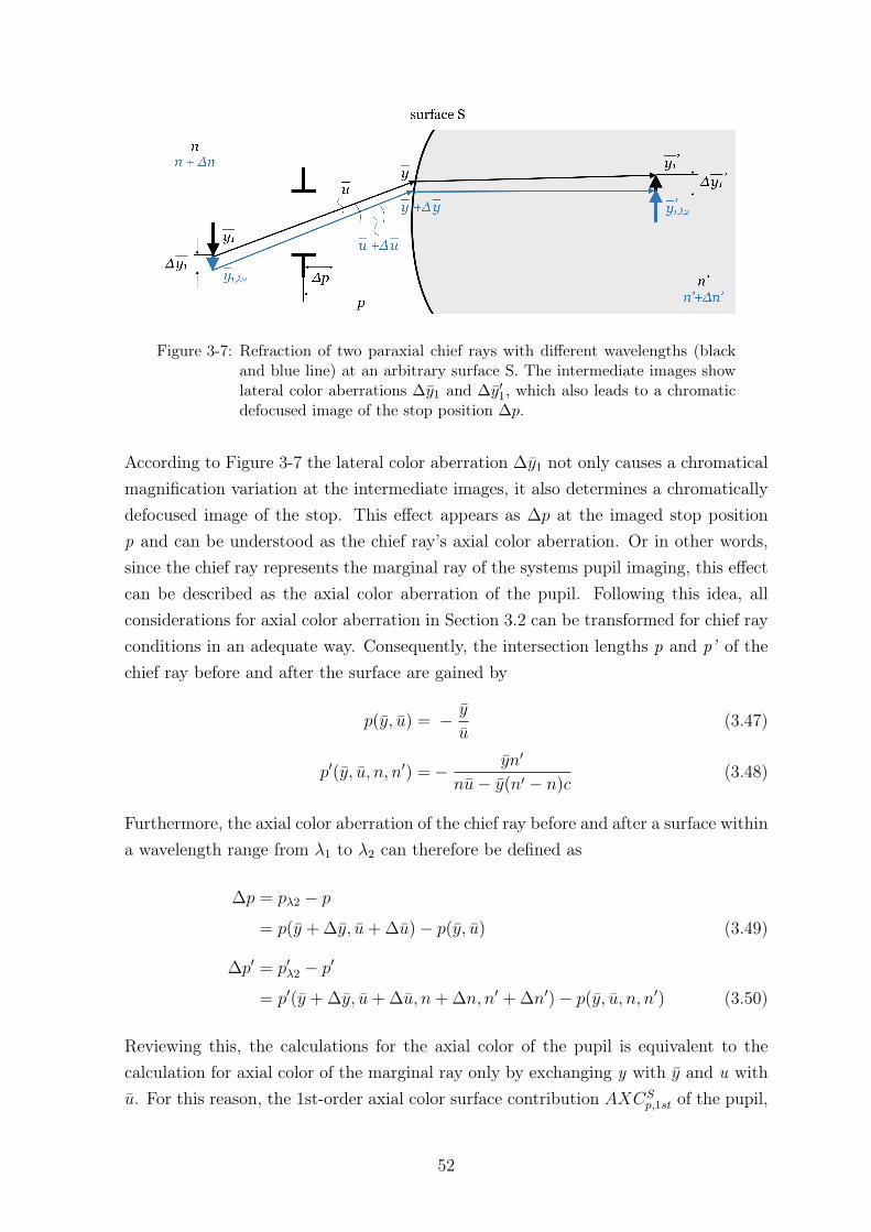
Figure 3-7: Refraction of two paraxial chief rays with different wavelengths (blackand blue line) at an arbitrary surface S. The intermediate images showlateral color aberrations Δ𝑦1 and Δ𝑦′1, which also leads to a chromaticdefocused image of the stop position Δ𝑝.

According to Figure 3-7 the lateral color aberration ∆𝑦1 not only causes a chromaticalmagnification variation at the intermediate images, it also determines a chromaticallydefocused image of the stop. This effect appears as ∆𝑝 at the imaged stop positionp and can be understood as the chief ray’s axial color aberration. Or in other words,since the chief ray represents the marginal ray of the systems pupil imaging, this effectcan be described as the axial color aberration of the pupil. Following this idea, allconsiderations for axial color aberration in Section 3.2 can be transformed for chief rayconditions in an adequate way. Consequently, the intersection lengths p and p’ of thechief ray before and after the surface are gained by

𝑝(𝑦, �̄�) = − 𝑦

�̄�(3.47)

𝑝′(𝑦, �̄�, 𝑛, 𝑛′) = − 𝑦𝑛′

𝑛�̄�− 𝑦(𝑛′ − 𝑛)𝑐(3.48)

Furthermore, the axial color aberration of the chief ray before and after a surface withina wavelength range from 𝜆1 to 𝜆2 can therefore be defined as

∆𝑝 = 𝑝𝜆2 − 𝑝

= 𝑝(𝑦 + ∆𝑦, �̄� + ∆�̄�) − 𝑝(𝑦, �̄�) (3.49)

∆𝑝′ = 𝑝′𝜆2 − 𝑝′

= 𝑝′(𝑦 + ∆𝑦, �̄� + ∆�̄�, 𝑛 + ∆𝑛, 𝑛′ + ∆𝑛′) − 𝑝(𝑦, �̄�, 𝑛, 𝑛′) (3.50)

Reviewing this, the calculations for the axial color of the pupil is equivalent to thecalculation for axial color of the marginal ray only by exchanging y with 𝑦 and u with�̄�. For this reason, the 1st-order axial color surface contribution 𝐴𝑋𝐶𝑆

𝑝,1𝑠𝑡 of the pupil,

52

describing the chromatically defocused imaged stop p is found by

𝐴𝑋𝐶𝑆𝑝,1𝑠𝑡 = 𝑛�̄�𝑦

(︂∆𝑛′

𝑛′ − ∆𝑛

𝑛

)︂(3.51)

Consequently, also the corresponding description of the chief ray’s preexisting 1st-orderaxial color aberration 𝐴𝑋𝐶𝑝,1𝑠𝑡 in front of the surface can be found by equation (3.52).

𝐴𝑋𝐶𝑝,1𝑠𝑡 = ∆𝑝1𝑠𝑡(−𝑛�̄�2) = 𝑛�̄�∆𝑦 − 𝑛𝑦∆�̄� (3.52)

Combining Equation (3.45) and (3.52) reveals the eliminating of ∆�̄� within these tworelations:

𝑛∆�̄� =−𝐴𝑋𝐶𝑝,1𝑠𝑡 + 𝑛�̄�∆𝑦

𝑦=

−𝐿𝐴𝐶1𝑠𝑡 + 𝑛𝑢∆𝑦

𝑦(3.53)

Reordering this leads to a new expression for 𝑛∆𝑦.

𝑛∆𝑦 =𝑦𝐴𝑋𝐶𝑝,1𝑠𝑡 − 𝑦𝐿𝐴𝐶1𝑠𝑡

𝑦�̄�− 𝑦𝑢(3.54)

Now, with this findings, the second term 𝑛𝑖∆𝑦(∆𝑛′/𝑛′−∆𝑛/𝑛) of Equation (3.46) andits single dependency on the chromatic difference of the chief ray height ∆𝑦 can simplybe rewritten by inserted (3.54) into Equation (3.46). This results in a new expressionfor 2nd-order lateral color surface contribution 𝐿𝐴𝐶𝑆

2𝑛𝑑 with all terms depending eitheron preexisting lower-order aberration or pure dispersive effects:

𝐿𝐴𝐶𝑆2𝑛𝑑 = 𝐿𝐴𝐶1𝑠𝑡

(︂∆𝑛′

𝑛′ − ∆𝑛

𝑛

)︂+

𝑖𝑦𝐴𝑋𝐶𝑝,1𝑠𝑡 − 𝑖𝑦𝐿𝐴𝐶1𝑠𝑡

𝑦�̄�− 𝑦𝑢

(︂∆𝑛′

𝑛′ − ∆𝑛

𝑛

)︂

− 𝑛�̄�𝑦

(︂∆𝑛′2

𝑛′2 − ∆𝑛∆𝑛′

𝑛𝑛′

)︂(3.55)

Rearranging and simplifying leads to a formula with only two terms left. Hence, thefinal description of 2nd-order lateral color surface contribution 𝐿𝐴𝐶𝑆

2𝑛𝑑 is obtained by

𝐿𝐴𝐶𝑆2𝑛𝑑 =

𝑦(𝑖𝐴𝑋𝐶𝑝,1𝑠𝑡 − �̄�𝐿𝐴𝐶1𝑠𝑡)

𝑦�̄�− 𝑦𝑢

(︂∆𝑛′

𝑛′ − ∆𝑛

𝑛

)︂− 𝑛�̄�𝑦

(︂∆𝑛′2

𝑛′2 − ∆𝑛∆𝑛′

𝑛𝑛′

)︂(3.56)

This equation is the second main result of this thesis.

3.3.2 Lens Contribution of Intrinsic and Induced Lateral Color

Since all of the considerations for the surface resolved lateral color can also be used fora thin lens description analog to [Nob15], the equivalent thin lens contribution formula

53

of 2nd-order lateral color is obtained by Equation (3.57).

𝐿𝐴𝐶𝐿2𝑛𝑑 =

𝑦∆𝐹𝐿

𝑦�̄�− 𝑦𝑢(𝑦𝐴𝑋𝐶𝑝,1𝑠𝑡 − 𝑦𝐿𝐴𝐶1𝑠𝑡) (3.57)

In contrast, the parameters for a thick lens formula in air are shown in Figure 3-8.

Figure 3-8: Refraction of the marginal ray and chief ray (dashed and solid line) at a thicklens with an refractive index of n. The marginal ray heights and angles are 𝑦1 and𝑢1 as well as 𝑦2 and 𝑢2 at surface S1 and surface S2, respectively. The chief rayheights and angles are 𝑦0 and �̄�0, 𝑦1 and �̄�1 as well as 𝑦2 and �̄�2 at the intermediateimage, surface S1 and surface S2, respectively.

Considering a certain thickness t for an individual lens in an optical system, the 2nd-order lateral color thick lens contribution 𝐿𝐴𝐶𝑡𝐿

2𝑛𝑑 can be calculated by the sum of bothsurface contributions:

𝐿𝐴𝐶𝑡𝐿2𝑛𝑑 = 𝐿𝐴𝐶𝑆1

2𝑛𝑑 + 𝐿𝐴𝐶𝑆22𝑛𝑑(𝑡) (3.58)

The surface contribution 𝐿𝐴𝐶𝑆12𝑛𝑑 of surface S1 is

𝐿𝐴𝐶𝑆12𝑛𝑑 =

𝑦1(𝑖1𝐴𝑋𝐶𝑝,1𝑠𝑡 − �̄�1𝐿𝐴𝐶1𝑠𝑡)

𝑦1�̄�0 − 𝑦1𝑢0

(︂∆𝑛

𝑛

)︂− 𝑛�̄�1𝑦1

(︂∆𝑛2

𝑛2

)︂(3.59)

and the surface contribution 𝐿𝐴𝐶𝑆22𝑛𝑑 of surface S2 is

𝐿𝐴𝐶𝑆22𝑛𝑑 =

𝑦2(𝑖2𝐴𝑋𝐶𝑝,1𝑠𝑡 − �̄�2𝐿𝐴𝐶1𝑠𝑡)

𝑦2�̄�1 − 𝑦2𝑢1

(︂−∆𝑛

𝑛

)︂(3.60)

Here, the preexisting 1st-order chromatic variation of magnification at the intermediateimage in front of surface S1 is assumed to 𝐿𝐴𝐶1𝑠𝑡. According to the Seidel surfacecoefficient 𝐶2 (Section 2.3.2), for surface S2 the preexisting 1st-order lateral color can

54

be calculated by:

𝐿𝐴𝐶 ′1𝑠𝑡 = 𝐿𝐴𝐶1𝑠𝑡 + �̄�1𝑦1∆𝑛/𝑛 (3.61)

Equivalent considerations have to be done for the chromatically defocused image of thestop. Here, the axial color of the imaged stop in front of surface S1 is considered to be𝐴𝑋𝐶𝑝,1𝑠𝑡. Following Equation (3.51) , the preexisting axial color of the chief ray forsurface S2 can be obtained by:

𝐴𝑋𝐶 ′𝑝,1𝑠𝑡 = 𝐴𝑋𝐶𝑝,1𝑠𝑡 + �̄�1𝑦1∆𝑛/𝑛 (3.62)

The influence of the lens’ thickness is represented by 𝑦2(𝑡), 𝑦2(𝑡), 𝑖2(𝑡) and �̄�2(𝑡). Insert-ing now Equation (3.59) and (3.60) into Equation (3.58) and rearranging as well assimplifying it, the following thick lens formula is achieved:

𝐿𝐴𝐶𝑡𝐿2𝑛𝑑 = − 𝑦1(𝑐1 − 𝑐2)∆𝑛

𝑦1�̄�0 − 𝑦1𝑢0

(︂𝑦1𝐴𝑋𝐶𝑝,1𝑠𝑡 − 𝑦1𝐿𝐴𝐶1𝑠𝑡

)︂

+ 𝑡𝛽1∆𝑛

𝑦1�̄�0 − 𝑦1𝑢0

𝐴𝑋𝐶𝑝,1𝑠𝑡 + 𝑡𝛽2∆𝑛

𝑦1�̄�0 − 𝑦1𝑢0

𝐿𝐴𝐶1𝑠𝑡

+ 𝑡�̄�1∆𝑛2(𝛽1𝑦1 + 𝛽2𝑦1)

𝑛(𝑦1�̄�0 − 𝑦1𝑢0)(3.63)

The coefficients 𝛽1 and 𝛽2 can be found in the appendix. Now, considering the relation∆𝐹𝑡𝐿 = ∆𝑛(𝑐1𝑐2) and the definition of the Lagrange Invariant 𝐻 = 𝑛(𝑦�̄� − 𝑦𝑢) ofSection 2.1.3, the following final result for the thick lens formula is obtained:

𝐿𝐴𝐶𝑡𝐿2𝑛𝑑 = − 𝐿𝐴𝐶𝐿

2𝑛𝑑 + 𝑡𝛽1𝑛∆𝑛

𝐻𝐴𝑋𝐶𝑝,1𝑠𝑡 + 𝑡𝛽2

𝑛∆𝑛

𝐻𝐿𝐴𝐶1𝑠𝑡 + 𝑡

�̄�1∆𝑛2(𝛽1𝑦1 + 𝛽2𝑦1)

𝐻(3.64)

3.3.3 Discussion

In case of 2nd-order lateral color surface contributions, Equation (3.56) was obtainedby a Taylor expansion up to 2nd-order considering a differentiation with respect todispersion. Here, the 2nd-order effects are expressed by two terms.

Induced and Intrinsic Terms The first term depends on the preexisting 1st-orderlateral color aberration in front of the surface, expressed by the chromatic variation ofmagnification at the intermediate image 𝐿𝐴𝐶1𝑠𝑡 supplemented with the chromaticallydefocused image of the stop 𝐴𝑋𝐶𝑝,1𝑠𝑡. Considering the definition and characteristicsof induced color aberrations, introduced in Section 3.1, this term describes clearly an

55

induced effect, as it would vanish, if there is no preexisting lateral color or axial colorof the pupil. In contrast to this, the second term only shows dependencies on thechromatic variation of the refractive indices before and after the surface ∆𝑛 and∆𝑛′ .Therefore, this term is an intrinsic term of 2nd-order.Analyzing the two terms of Equation (3.56) in detail, a linear dependency of the firstterm on the preexisting lateral color described by (𝑖𝐴𝑋𝐶𝑝,1𝑠𝑡 − �̄�𝐿𝐴𝐶1𝑠𝑡) is found.Furthermore, since also the dispersion factor (∆𝑛′/𝑛′ − ∆𝑛/𝑛) is present, this termspecifies the interaction between the preexisting summed up 1st-order lateral coloreffects with a dispersive acting surface. As it is the only induced term, a mirror cannotproduce any induced lateral color effects.Comparing the last term −𝑛�̄�𝑦(Δ𝑛′2

𝑛′2 − Δ𝑛Δ𝑛′

𝑛𝑛′ ) of Equation (3.56) with the last term−𝑛𝑖𝑦(Δ𝑛′2

𝑛′2 − Δ𝑛′Δ𝑛𝑛′𝑛

) of the 2nd-order axial color contribution, the calculation for thelateral color term is equivalent to the calculation for the axial color term only byexchanging i with �̄�. Hence, this term shows again a dependence on the individualsurface type. If it is a back surface in air, this term vanishes, as ∆𝑛′ for air is zero.But if it is a cemented surface or a front surface in air, this term introduces a certain2nd-order contribution to lateral color. Therefore, for the lens resolved approach thisterm vanishes analog to the fourth term of 2nd-order axial color.

Required Parameters Due to the additional consideration of the pupil axial coloraberration effect, again the calculation of all required quantities by only one paraxialraytrace is enabled. Following the Seidel sum definition for lateral color (2.50) andthe new found relation of (3.51), any preexisting 1st-order lateral color 𝐿𝐴𝐶1𝑠𝑡 and1st-order axial color of the pupil 𝐴𝑋𝐶𝑝,1𝑠𝑡 before an individual surface 𝑆𝑗 can easilybe calculated by summing up all 1st-order surface contributions up to surface 𝑆𝑗−1 by:

𝐿𝐴𝐶1𝑠𝑡 =

𝑗−1∑︁𝑎=1

𝐿𝐴𝐶𝑆1𝑠𝑡

=

𝑗−1∑︁𝑎=1

𝑛𝑎𝑦𝑎�̄�𝑎

(︂∆𝑛′

𝑛′ − ∆𝑛

𝑛

)︂𝑎

(3.65)

𝐴𝑋𝐶𝑝,1𝑠𝑡 =

𝑗−1∑︁𝑎=1

𝐴𝑋𝐶𝑆𝑝,1𝑠𝑡

=

𝑗−1∑︁𝑎=1

𝑛𝑎𝑦𝑎�̄�𝑎

(︂∆𝑛′

𝑛′ − ∆𝑛

𝑛

)︂𝑎

(3.66)

56

Therefore, all terms in Equation (3.56) are determined by paraxial marginal and chiefray data for the reference wavelength only. Hence, a single paraxial raytrace for thereference wavelength provides all required parameters for calculating the 2nd-orderlateral color effects. An additional raytrace for another wavelength is again not needed.

The Role of the Real Stop Furthermore, just as for 1st-order lateral color, thelocation of the real stop within an optical system influences the amount of 2nd-order,too. For 2nd-order lateral color this influence of the real stop position is representedby 𝐴𝑋𝐶𝑝,1𝑠𝑡. For every surface in an optical system an intermediate image formed bythe preceding optical elements can be determined. For lateral color, additionally theimage of the real stop, seen from that intermediate image has to be considered. Aslong as the chief ray hits the optical axis at an image of the stop, a certain amount of𝐴𝑋𝐶𝑝,1𝑠𝑡 will be identified. But in case of the real stop position, the axial color of thechief ray 𝐴𝑋𝐶𝑝,1𝑠𝑡 will be zero by definition at the location of the stop, as for everywavelength the chief ray will pass through the center of it. Hence, in optical systemswith a front stop arrangement 𝐴𝑋𝐶𝑝,1𝑠𝑡 sums up surface by surface. However, a setupwith a real stop within the optical system shows a certain off-set of 𝐴𝑋𝐶𝑝,1𝑠𝑡 in frontof the first surface, which then sums up surface by surface to zero until the real stopis reached. Hence, for the front part of the system the summation 𝐴𝑋𝐶𝑝,1𝑠𝑡 has to bedone in the opposite direction starting at the real stop position.

Lens Contribution The considerations for the thick lens resulting in Equation(3.64) again confirms two facts. On the one hand the compensating effect of theintrinsic term in Equation (3.56) is shown, as there is no 2nd-order intrinsic term leftin the equation, independent of the thickness t. This intrinsic term is canceling out byrearranging and simplifying Equation (3.58). On the other hand, the expected relationbetween the thin lens formula and the thick lens approach was shown again. In case of2nd-order lateral color the thick lens formula consists of four summands, the thin lenscontribution of Equation (3.57) and three thickness depending terms. Here, the latterone can again be divided in two thickness depending induced terms, 𝑡𝑏1 𝑛Δ𝑛

𝐻𝐴𝑋𝐶𝑝,1𝑠𝑡

as well as +𝑡𝑏2𝑛Δ𝑛𝐻

𝐿𝐴𝐶1𝑠𝑡 , and one thickness depending intrinsic term 𝑡 �̄�1Δ𝑛2(𝑏1𝑦1+𝑏2𝑦1)𝐻

.

57

3.4 Induced Spherochromatism

3.4.1 Definition of Spherochromatism

In this section, the paraxial region of axial and lateral color is left by increasing theaberration’s order of pupil dependency obtaining spherical aberration and its chromaticvariation. In general, spherochromatism is defined as the chromatic variation of spher-ical aberration. Therefore, the analytical description of spherical aberration representsthe initial point for this approach. There are several ways to obtain an exact expres-sion for spherical aberration at an arbitrary surface in an optical system describedin literature [Del52], [Ker95], [CK92]. An appropriate expression of [Del52]is shownin Equation (3.67). Additionally, Figure 3-9 illustrates the corresponding parametersdefining the spherical aberration conditions.

𝑆𝑃𝐻 ′ = 𝑆𝑃𝐻𝑛𝑢 sin𝑈

𝑛′𝑢′ sin𝑈 ′ +−4𝑛𝑖𝑟 sin( 𝐼−𝑈

2) sin( 𝐼−𝐼′

2)

𝑛′𝑢′ sin𝑈 ′ (3.67)

Here, a single refractive surface j with curvature c is hit by a paraxial and real marginalray. The paraxial and the real ray heights at the surface are y and Y, respectively. Theparaxial ray angle before the surface is determined by u, and the paraxial ray angleafter the surface is determined by u‘. Accordingly, the ray angles of the real ray beforeand after the surface are defined by U and U’. Furthermore, the equivalent incidentangles are described by i for the paraxial ray and I for the real ray. Consideringnow the different intersection lengths s and S of the paraxial marginal ray and thereal marginal ray, respectively, the longitudinal spherical aberration SPH before thesurface is obtained by the difference 𝑆𝑃𝐻 = 𝑆−𝑠. Similarly, the longitudinal sphericalaberration SPH’ at the intermediate image after the surface is represented by thecorresponding difference of the intersection lengths S’ and s’ of the real and paraxialray after the surface. (Figure 3-9)

Figure 3-9: Parameters defining the spherical aberration conditions. Here, capitalletters refer to real ray and small letter to the paraxial ray parameters.

58

Equation (3.67) now allows the exact calculation of SPH’ depending on the sphericalaberration in the preceding optical system SPH and the above described ray conditionsat an arbitrary surface. The first term of Equation (3.67) represents the longitudinalspherical aberration, transferred from the preceding system, in which the factor in frontof SPH describes the longitudinal magnification of the surface. However, the secondterm expresses the new longitudinal spherical aberration introduced by the surfaceitself. This term represents the relevant part for obtaining a single surface contributionformula.Considering now the definition of spherochromatism, the chromatic variation of theabove described parameters have to be included. Here, the first wavelength is assumedto be the reference wavelength 𝜆 = 𝜆1 . For a second wavelength 𝜆2 small differenceswithin the material’s refractive index ∆𝑛,∆𝑛′, in ray heights ∆𝑦,∆𝑌 and in ray angles∆𝑢,∆𝑈 for the paraxial as well as for the real marginal ray occur. Hence, for a secondwavelength different spherical aberration values before and after the surface as wellas the axial color between the two wavelengths affects the spherochromatism. This isshown in Figure 3-10.

Figure 3-10: Quantities defining spherochromatism. Here, the solid black line pa-rameters refer to the real ray path and dashed black line parameters tothe paraxial ray path of the primary wavelength 𝜆1. The second wave-length 𝜆2 is represented by blue lines. Again, capital letters belong tothe real rays and small letters to the paraxial rays.

In literature, no consistent procedure can be found how to deal with the axial colorcontribution. For example, Haferkorn [Haf86], Hofmann [Hof] and Smith [Smi04] in-clude axial color to the spherochromatism amount, but e.g. Kingslake [Kin12], Zimmer[Zim67] and Malacara [MM17] remove the axial color for their definitions. Since thisapproach is following the Seidel idea, where a surface contribution for axial color isalready existing and to ensurean independent evaluation of the spherical aberrationeffects, here the influence of the surface’s axial color will be neglected. Hence, thelongitudinal spherochromatism GA, named corresponding to its German expression

59

Gaußfehler, is defined as the difference of the longitudinal spherical aberration of dif-ferent wavelengths:

𝐺𝐴 = 𝑆𝑃𝐻𝜆2 − 𝑆𝑃𝐻𝜆1 (3.68)

Figure 3-11 illustrates this definition for the case, shown in Figure 3-10. Please notethat for spherochromatism GA and GA’ the axial color contribution is neglected.

Figure 3-11: Longitudinal aberration plot corresponding to the relations, shown inFigure 3-10 for wavelength 𝜆1 and wavelength 𝜆1. Here, the intersectionlength s for 𝜆1 provides the reference. Δ𝑠 describes the difference in z-direction to this reference and ℎ𝑝 characterizes the relative pupil height.

3.4.2 Surface Contribution of Intrinsic and Induced Spherochro-

matism

Following now Seidel’s approach, where the primary monochromatic aberrations areobtained by paraxial approximation of the rays, a 3rd-order spherochromatism willbe achieved by the chromatic variation of the paraxial rays, characterizing primaryspherical aberration. As mentioned before, the second term of the exact Equation(3.67) represents the relevant term for defining an exact single surface contributionformula of spherical aberration 𝑆𝑃𝐻𝑒𝑥𝑎𝑐𝑡

𝑗 :

𝑆𝑃𝐻𝑒𝑥𝑎𝑐𝑡𝑗 =

−4𝑛𝑖𝑟 sin( 𝐼−𝑈2

) sin( 𝐼−𝐼′

2)

𝑛′𝑢′ sin𝑈 ′ (3.69)

60

Considering this expression, the primary surface contribution for spherical aberrationis now obtained by assuming sin𝑥 = 𝑥 , by replacing the real ray data with theirparaxial ray data with 𝑈 = 𝑢, 𝑢′ = 𝑢′, 𝐼 = 𝑖, 𝐼 ′ = 𝑖′ and by taking the followingparaxial relations (2.5) and (2.6) of Section 2.1.2 as well as (2.12) of Section 2.1.3 intoaccount.Equation (3.70) shows the result for primary longitudinal spherical aberration surfacecontribution 𝑆𝑃𝐻 ′

𝑗. Here, 𝑆𝐼 describes the Seidel coefficient for spherical aberration.The expression 1

2𝑛′𝑢′2 is the conversion factor for the longitudinal description of thewavefront aberration 𝑆𝐼 .

𝑆𝑃𝐻𝑗 =1

2𝑛′𝑢′2 𝑛2𝑖2𝑦

(︂𝑢′

𝑛′ −𝑢

𝑛

)︂=

−𝑆𝐼

2𝑛′𝑢′2 (3.70)

For a 3rd-order chromatic variation approach, the Seidel coefficient 𝑆𝐼 = −𝑛2𝑖2𝑦(𝑢′

𝑛′ −𝑢𝑛) represents the basic relation to investigate for different wavelengths. Hence, an

expression depending only on ray heights, angles and the refractive index is requiredand can be obtained by applying the paraxial relation for the incident angle 𝑖 = 𝑢+ 𝑦𝑐

and the raytrace equation 𝑛′𝑢′ = 𝑛𝑢− 𝑦𝑐(𝑛′ − 𝑛):

𝑆𝐼(𝑢, 𝑦, 𝑛, 𝑛′) = −𝑦(𝑛2 − 𝑛′𝑛)(𝑢 + 𝑦𝑐)2(𝑛𝑢 + 𝑛′𝑢 + 𝑦𝑐𝑛)

𝑛′2 (3.71)

Considering now a second wavelength 𝜆2 = 𝜆1 + ∆𝜆, the corresponding paraxial rayheight at the surface is 𝑦2 = 𝑦+ ∆𝑦 and the corresponding ray angle before the surfaceis𝑢2 = 𝑢+ ∆𝑢. Similarly to this, also the refractive indices show a wavelength depend-ing, dispersive behavior, considered by 𝑛2 = 𝑛 + ∆𝑛 and 𝑛′

2 = 𝑛′ + ∆𝑛′. Therefore,thechromatic variation ∆𝑆𝐼 of the Seidel coefficient, within a wavelength range from 𝜆2

to 𝜆1 represents the Seidel equivalent surface coefficient for spherochromatism 𝐺𝑆 andcan be defined by

𝐺𝑆 = ∆𝑆𝐼 = 𝑆𝐼,𝜆2 − 𝑆𝐼,𝜆1

= 𝑆𝐼(𝑢 + ∆𝑢, 𝑦 + ∆𝑦, 𝑛 + ∆𝑛, 𝑛′ + ∆𝑛′) − 𝑆𝐼(𝑢, 𝑦, 𝑛, 𝑛′) (3.72)

Equally to the Seidel coefficient 𝑆𝐼 , also the here described spherochromatism co-efficient G is expressed in effective wavefront aberration. Now, if the differences∆𝑢,∆𝑦,∆𝑛 and ∆𝑛′ are small, a Taylor expansion of 1st-order yields to the following

61

expression for the Seidel coefficient 𝑆𝐼,𝜆2 of the second wavelength:

𝑆𝐼,𝜆2 = 𝑆𝐼(𝑢 + ∆𝑢, 𝑦 + ∆𝑦, 𝑛 + ∆𝑛, 𝑛′ + ∆𝑛′)

= 𝑆𝐼(𝑢, 𝑦, 𝑛, 𝑛′) +

𝜕𝑆1

𝜕𝑦∆𝑦 +

𝜕𝑆1

𝜕𝑢∆𝑢 +

𝜕𝑆1

𝜕𝑛∆𝑛′ +

𝜕𝑆1

𝜕𝑛′ ∆𝑛′ (3.73)

Corresponding to Equation (3.72) the Seidel equivalent surface contribution of sphe-rochromatism 𝐺𝑆 is given by:

𝐺𝑆 =𝜕𝑆1

𝜕𝑦∆𝑦 +

𝜕𝑆1

𝜕𝑢∆𝑢 +

𝜕𝑆1

𝜕𝑛∆𝑛′ +

𝜕𝑆1

𝜕𝑛′ ∆𝑛′ (3.74)

The partial derivatives required for 𝐺𝑆 can be found in the appendix. Considering thoseand the paraxial relations of mentioned before, an expression for the spherochromatismsurface contribution 𝐺𝑆 is obtained:

𝐺𝑆 = ∆𝑦(𝑢− 𝑢′)(−4𝑛′𝑖2 − 𝑛𝑢2 + 3𝑛𝑢𝑢′)

+ ∆𝑢𝑦(𝑢− 𝑢′)(−4𝑛′𝑖 + 𝑛𝑢− 3𝑛𝑢′)

+ ∆𝑛𝑖𝑦(𝑖′2 − 𝑖′𝑢 + 2𝑖′𝑢′ − 𝑢2 + 𝑢𝑢′)

+ ∆𝑛′𝑖′2𝑦(𝑢′ − 𝑖′) (3.75)

Here, two terms depending on the dispersive behavior of the materials before and afterthe surface, represented by ∆𝑛 and ∆𝑛′, can be found. But additionally, also bothterms depending on the chromatic variation of the paraxial marginal ray angle ∆𝑢

and the paraxial marginal ray height ∆𝑦 remain after expansion. In contrast to the1st-order derivatives of axial color and lateral color in Section 3.2.1 and 3.3.1, theseterms do not cancel out for the chromatic variation of Seidel’s spherical aberrationcoefficient.Following now the idea of induced aberrations, some of the four terms in Equation(3.75) have to depend on the cumulative preexisting lower-order color aberrations ofthe system before. Since here the marginal ray’s chromatic variation occurs, 1st-orderaxial color is investigated. For the preexisting axial color AXC in front of a surface, anexpression, including the marginal ray’s ∆𝑢 and ∆𝑦, was already described in (3.17):

𝐴𝑋𝐶1𝑠𝑡 = 𝑛𝑢∆𝑦 − 𝑛𝑦∆𝑢 (3.76)

Analyzing the spherochromatism terms of Equation (3.75) for a dependency on Equa-tion (3.76), shows that 𝐺𝑆 cannot be described with the help of axial color only. Hence,to specify all paraxial effects of a chromatically varying marginal ray, the approach hasto be extended. Figure 3-12, shows the additional considerations.

62

Figure 3-12: Extended considerations on a chromatically varying marginal ray. Here, thesolid line parameters again refer to the marginal ray of the primary wavelength𝜆1 and the blue line parameters to the marginal ray of the second wavelength𝜆2. Additionally, the chief ray of 𝜆1 is plotted as a dotted line. The intersectionlength s of the marginal ray characterizes the intermediate image for 𝜆1. At thisimage, an axial color aberration Δ𝑠 is present. The position of the imaged stopin front of the surface is defined by the intersection length p of the chief ray.Here, a chromatic varying stop size characterized by Δ𝑦𝑝 is present. The sameconsiderations are applied for the primed quantities after the surface.

The relations shown in Figure 3-12 describe the consequent extension of the very simi-lar approach of Section 3.3.1. In contrast to this, here the influence of a chromaticallyvarying marginal ray on the imaged stop is considered. According to Figure 3-12, thecolor variation of the marginal ray not only causes a chromatic difference in imageposition, which is described by the axial color amount ∆𝑠 at the intermediate image,it also generates a chromatically varying imaged stop size ∆𝑦𝑝. Since the marginal rayrepresents the chief ray of the systems pupil imaging, this effect can be understood asa lateral color aberration at the imaged stop position p. Hence, this extended consid-eration on a chromatically varying marginal ray, allows a description of all chromaticeffects by two individual quantities, the axial color at the intermediate image and thelateral color of the pupil image.For the axial color, the common used Seidel surface contribution formula 𝐶1 (Section2.3.1, Equation (2.46)) as well as Equation (3.76) can be applied. For the lateral colorof the stop image, the considerations for 2nd-order lateral color derived in Section3.3.1 can be adopted, but have to be transformed for the above explained marginal rayconditions in an adequate way. Therefore, the ray heights of the marginal ray at theimaged stop position, 𝑦𝑝 and ∆𝑦′𝑝, before and after the surface are obtained by:

𝑦𝑝(𝑦, 𝑢) = 𝑦 + 𝑝𝑢 (3.77)

𝑦′𝑝(𝑦, 𝑢, 𝑛, 𝑛′) = 𝑦 + 𝑝′

𝑛𝑢− 𝑦𝑐(𝑛′ − 𝑛)

𝑛′ (3.78)

63

Here, the imaged stop positions p and p’ can be understood as the intersection lengthsof the chief ray, which is characterized by its ray height 𝑦 and its ray angle �̄�. (3-12)Hence, they are found by:

𝑝(𝑦, 𝑢) = − 𝑦

𝑢(3.79)

𝑝′(𝑦, 𝑢, 𝑛, 𝑛′) = − 𝑦𝑛′

𝑛�̄�− 𝑦𝑐(𝑛′ − 𝑛)(3.80)

Now, the lateral color aberration of the imaged stop before and after a surface, ∆𝑦𝑝

and ∆𝑦′𝑝, within a wavelength range from 𝜆1 to 𝜆2, is defined by the difference of thetwo stop sizes for 𝜆1 and 𝜆2. Here, again the chromatic variation in ray angle ∆𝑢, rayheight ∆𝑦 and for the material’s refractive index, and ∆𝑛 and and ∆𝑛′, are included:

∆𝑦𝑝 = 𝑦𝑝,𝜆2 − 𝑦𝑝,𝜆1

= 𝑦𝑝(𝑦 + ∆𝑦, 𝑢 + ∆𝑢) − 𝑦𝑝(𝑦, 𝑢) (3.81)

∆𝑦′𝑝 = 𝑦′𝑝,𝜆2 − 𝑦′𝑝,𝜆1

= 𝑦′𝑝(𝑦 + ∆𝑦, 𝑢 + ∆𝑢, 𝑛 + ∆𝑛, 𝑛′ + ∆𝑛′) − 𝑦′𝑝(𝑦, 𝑢, 𝑛, 𝑛′) (3.82)

Reviewing this, the calculations for the lateral color of pupil image is equivalent tothe calculation for the lateral color of the object, only by exchanging 𝑦 withy and 𝑦

with u.For this reason, the surface contribution for the lateral color of the imaged stop𝐿𝐴𝐶𝑆

𝑝 as well as the corresponding expression for the preexisting amount in front of asurface 𝐿𝐴𝐶𝑝, can easily be obtained by the same exchange of ray data. For 𝐿𝐴𝐶𝑆

𝑝 ,this exchange is applied to Seidel’s well-known surface contribution formula for lateralcolor 𝐶2 (Section 2.3.2, Equation (2.50)). The result is shown in Equation (3.83).

𝐿𝐴𝐶𝑆𝑝,1𝑠𝑡 = 𝑛𝑖𝑦

(︂∆𝑛′

𝑛′ − ∆𝑛

𝑛

)︂(3.83)

Furthermore, after exchanging the chief ray data with the marginal ray data of Equation(3.45) to obtain 𝐿𝐴𝐶𝑝, the relation shown in (3.84), depending on ∆𝑢 and ∆𝑦 is found:

𝐿𝐴𝐶𝑝,1𝑠𝑡 = 𝑛�̄�∆𝑦 − 𝑛𝑦∆𝑢 (3.84)

Coming back to the Seidel equivalent spherochromatism coefficient 𝐺𝑆(∆𝑦,∆𝑢,∆𝑛,∆𝑛′),derived in Equation(3.75), the remaining dependency on the chromatic variation of theparaxial marginal ray angle ∆𝑢 and ray height∆𝑦 can be expressed by combining Equa-tion (3.76) and (3.84). This is carried out by rearranging the formulas for 𝐴𝑋𝐶1𝑠𝑡 and

64

𝐿𝐴𝐶𝑝,1𝑠𝑡 in the following way.

∆𝑦 =𝐴𝑋𝐶1𝑠𝑡 + 𝑛𝑦∆𝑢

𝑛𝑢=

𝐿𝐴𝐶𝑝,1𝑠𝑡 + 𝑛𝑦∆𝑢

𝑛�̄�(3.85)

∆𝑢 =−𝐴𝑋𝐶1𝑠𝑡 + 𝑛𝑢∆𝑦

𝑛𝑦=

−𝐿𝐴𝐶𝑝,1𝑠𝑡 + 𝑛�̄�∆𝑦

𝑛𝑦(3.86)

Considering these relations,∆𝑢 and ∆𝑦 can be rewritten as shown in Equation (3.87)and (3.88) . Please again note, 𝐴𝑋𝐶1𝑠𝑡 represents the cumulative summed up 1st-orderaxial color Seidel coefficients in front of the surface, 𝐿𝐴𝐶𝑝,1𝑠𝑡 the summed up 1st-orderlateral color of the imaged stop in front of the surface and H the Lagrange Invariantwith 𝐻 = 𝑛�̄�𝑦 − 𝑛𝑢𝑦.

∆𝑢 =𝑢𝐿𝐴𝐶𝑝,1𝑠𝑡 − �̄�𝐴𝑋𝐶1𝑠𝑡

𝑛�̄�𝑦 − 𝑛𝑢𝑦=

𝑢𝐿𝐴𝐶𝑝,1𝑠𝑡 − �̄�𝐴𝑋𝐶1𝑠𝑡

𝐻(3.87)

∆𝑦 =𝑦𝐿𝐴𝐶𝑝,1𝑠𝑡 − 𝑦𝐴𝑋𝐶1𝑠𝑡

𝑛�̄�𝑦 − 𝑛𝑢𝑦=

𝑦𝐿𝐴𝐶𝑝,1𝑠𝑡 − 𝑦𝐴𝑋𝐶1𝑠𝑡

𝐻(3.88)

These two Equations now represent the missing relations to allow all terms of 𝐺𝑆 todepend either on preexisting lower-order color aberration or pure dispersive effects.Hence, inserting them into Equation (3.75) results in a new expression for a 3rd-orderSeidel equivalent spherochromatism surface contribution 𝐺𝑆:

𝐺𝑆 = (𝑦𝐴𝑋𝐶1𝑠𝑡 − 𝑦𝐿𝐴𝐶𝑝,1𝑠𝑡)4𝑖𝑛

𝐻(𝑢− 𝑢′)(𝑖 + 𝑢′)

− 𝐴𝑋𝐶1𝑠𝑡(𝑢− 𝑢′)(𝑢′ − 3𝑢− 4𝑖′)

− ∆𝑛𝑖𝑦(︀(𝑢′ − 𝑢)2 − (𝑖′ + 𝑢′)2 + 𝑢(𝑖′ + 𝑢′)

)︀− ∆𝑛′𝑖′2𝑦(𝑖′ + 𝑢′) (3.89)

This equation is the third main result of this thesis.

3.4.3 Thin Lens Contribution of Intrinsic and Induced Sphe-

rochromatism

To analyze the effect of spherochromatism in compound systems, also a contributionformula for a thin lens in air is investigated. For spherochromatism, this lens contri-bution can again be derived by the sum of both thin lens’ surface contributions:

𝐺𝐿 = 𝐺𝑆1 + 𝐺𝑆2 (3.90)

65

Here, the surface contribution 𝐺𝑆1 of the this lens’ first surface S1 equals to Equation(3.91), considering 𝑛 = 0 and ∆𝑛 = 0, since the lens is assumed to be in air. Thetwo material characterizing quantities of the thin lens’ glass are the refractive index𝑛′ = 𝑛𝐿 and its dispersive quantity ∆𝑛′ = ∆𝑛′

𝐿.

𝐺𝑆1 = (𝑦𝐴𝑋𝐶𝑆11𝑠𝑡 − 𝑦𝐿𝐴𝐶𝑆1

𝑝,1𝑠𝑡)4𝑖0𝐻

(𝑢0 − 𝑢′0)(𝑖0 + 𝑢′

0)

− 𝐴𝑋𝐶𝑆11𝑠𝑡(𝑢0 − 𝑢′

0)(𝑢′0 − 3𝑢0 − 4𝑖′0)

− ∆𝑛′𝑖′2𝑦(𝑖′ + 𝑢′) (3.91)

𝐴𝑋𝐶𝑆11𝑠𝑡 and 𝐿𝐴𝐶𝑆1

𝑝,1𝑠𝑡 are the prior summed up 1st-order color aberrations in front ofthe thin lens.Consequently, the second surface contribution 𝐺𝑆2 of the thin lens’ second surface S2is obtained by:

𝐺𝑆2 = (𝑦𝐴𝑋𝐶𝑆21𝑠𝑡 − 𝑦𝐿𝐴𝐶𝑆2

𝑝,1𝑠𝑡)4𝑖1𝑛𝐿

𝐻(𝑢1 − 𝑢′

1)(𝑖1 + 𝑢′1)

− 𝐴𝑋𝐶𝑆21𝑠𝑡(𝑢1 − 𝑢′

1)(𝑢′1 − 3𝑢1 − 4𝑖′1)

− ∆𝑛𝑖1𝑦(︀(𝑢′

1 − 𝑢1)2 − (𝑖′1 + 𝑢′

1)2 + 𝑢1(𝑖

′1 + 𝑢′

1))︀

(3.92)

Please note, the ray heights y and 𝑦 do not differ from surfaces S1 to surface S2, sincea negligible thickness is assumed. Concerning the incident and emergent angles as wellas the ray angle before and after the surfaces, the index 0 refer to the angles in frontof surface S1 and the index 1 to the angles in front of surface S2. Now, consideringthe paraxial relations (2.5) and (2.6) of Section 2.1.2 as well as the ray trace Equation(2.12) of Section 2.1.3, the different angles at surface S2 can simply be calculated fromthe given angles at surface S1. As a result of this and referring to the Seidel axial colorsurface contribution 𝐶1 (Section 2.3.1, Equation (2.46)) and Equation (3.83) for thesurface contribution of 𝐿𝐴𝐶𝑝,1𝑠𝑡, the prior summed up axial color at the second surfaceis equal to 𝐴𝑋𝐶𝑆2

1𝑠𝑡 = 𝐴𝑋𝐶1𝑠𝑡 − 𝑛𝐿𝑖1𝑦∆𝑛𝐿/𝑛𝐿 and the prior summed up lateral colorof the pupil at the second surface is equal to 𝐿𝐴𝐶𝑆2

𝑝,1𝑠𝑡 = 𝐿𝐴𝐶𝑝,1𝑠𝑡 − 𝑛𝐿𝑖1𝑦∆𝑛𝐿/𝑛𝐿 .With those considerations and by inserting Equation (3.92) and (3.91) into Equation(3.90), the final thin lens spherochromatism formula is obtained by:

𝐺𝐿 = (𝑦𝐴𝑋𝐶1𝑠𝑡 − 𝑦𝐿𝐴𝐶𝑝,1𝑠𝑡)4𝑦𝐹

𝐻𝑛𝐿

𝛾1 + 𝐴𝑋𝐶1𝑠𝑡𝑦𝐹

𝑛𝐿

𝛾2 + ∆𝑛𝐿𝑦2

𝑛2𝐿

(𝑐1 − 𝑐2)𝛾3 (3.93)

Here, F is the refractive power of the thin lens shown in Section 2.1.4 by Equa-tion (2.22).The coefficients 𝛾1(𝑖0, 𝑢0, 𝑖

′1, 𝑛𝐿),𝛾2(𝑖0, 𝑢0, 𝑖

′1, 𝑛𝐿) and 𝛾3(𝑖0, 𝑢0, 𝑖

′1, 𝑛𝐿) can be

found in the appendix.

66

3.4.4 Discussion

The final equation for a 3rd-order Seidel equivalent spherochromatism surface contribu-tion is shown in Equation 65. It was obtained by a Taylor expansion of Seidel’s spher-ical aberration coefficient 𝑆𝐼 up to 1st–order concerning its dependency on wavelengthvariation. Equally to the Seidel coefficient 𝑆𝐼 , also the new found spherochromatismcoefficient G is given as an effective wavefront aberration.

Induced and Intrinsic Terms Here, G is expressed by four terms. The first twoterms depend on prior summed up 1st-order color effects, caused by the chromaticvariation of the marginal ray. In case of the first term, this is expressed by the factor(𝑦𝐴𝑋𝐶1𝑠𝑡 − 𝑦𝐿𝐴𝐶𝑝,1𝑠𝑡), including both, the prior summed up lateral color of the pupil𝐿𝐴𝐶𝑝,1𝑠𝑡 and the prior summed up axial color 𝐴𝑋𝐶1𝑠𝑡. In case of the second term,again the presence of the prior summed up axial color 𝐴𝑋𝐶1𝑠𝑡 indicates its dependencyon the chromatic variation of the marginal ray. Hence, these two terms show clearlyinduced characteristics, as they would vanish, if there is no preexisting axial color orlateral color of the imaged stop. In contrast to this, the third and fourth term showonly dependencies on the chromatic variation of the refractive indices before and afterthe surface ∆𝑛 and ∆𝑛′. Therefore, these terms are of intrinsic character, as theywould still be valid without any prior element in front of the investigated surface.

Required Parameters The extended considerations by including also the coloraberrations of the imaged stop besides the axial color, enables the calculation of allrequired quantities by only one paraxial raytrace through the optical system. Due toEquations 64 and the well-known Seidel sum for axial color 𝐶1 (Section 2.3.1, Equa-tion (2.46), the 1st-order color aberrations 𝐴𝑋𝐶1𝑠𝑡. and 𝐿𝐴𝐶𝑝,1𝑠𝑡 before an individualsurface j can easily be calculated by summing up all of their surface contributions upto surface 𝑗 − 1 by:

𝐴𝑋𝐶1𝑠𝑡 = 𝐶1

=

𝑗−1∑︁𝑎=1

𝑛𝑎𝑖𝑎𝑦𝑎

(︂∆𝑛′

𝑛′ − ∆𝑛

𝑛

)︂𝑎

(3.94)

𝐿𝐴𝐶𝑝,1𝑠𝑡 =

𝑗−1∑︁𝑎=1

𝐿𝐴𝐶𝑆𝑝,1𝑠𝑡

=

𝑗−1∑︁𝑎=1

𝑛𝑎𝑖𝑎𝑦𝑎

(︂∆𝑛′

𝑛′ − ∆𝑛

𝑛

)︂𝑎

(3.95)

67

Therefore, all terms of Equation (3.89) are determined by the marginal and chief raydata for the reference wavelength only. Hence, a single paraxial raytrace for the refer-ence wavelength provides all required parameters for calculating the 3rd -order sphe-rochromatism. An additional raytrace for another wavelength is not needed.

The Role of the Real Stop Just as known for higher-order spherical aberration[Haf86], the location of the real stop within an optical system influences the amountof 3rd- order spherochromatism, too. For spherochromatism this influence of the realstop position is represented by 𝐿𝐴𝐶𝑝,1𝑠𝑡. For every surface in an optical system anintermediate image formed by the preceding optical elements can be determined. Forspherochromatism, additionally the image of the real stop, seen from that intermediateimage has to be considered. As long as the chief ray hits the optical axis at an imageof the stop, a certain amount of 𝐿𝐴𝐶𝑝,1𝑠𝑡 will be identified. But in case of the real stopposition, the lateral color of the marginal ray 𝐿𝐴𝐶𝑝,1𝑠𝑡 will be zero by definition, asfor every wavelength the marginal ray will pass the stop at the rim. Hence, in opticalsystems with a front stop arrangement 𝐿𝐴𝐶𝑝,1𝑠𝑡 sums up surface by surface. However,a setup with a real stop within the optical system shows a certain off-set of 𝐿𝐴𝐶𝑝,1𝑠𝑡

in front of the first surface, which then sums up surface by surface to be zero until thereal stop is reached.

Longitudinal Spherochromatism Contribution Since the contribution of G wasderived from Seidel’s spherical aberration coefficient 𝑆𝐼 , also Equation (3.89) and all ofthe previous expressions of G give the spherochromatism surface contribution in termsof wavefront aberrations. Please note, likewise the Seidel aberrations, this is essen-tially a wavefront aberration. E.g.,the scaling factor of 1/8 relates Seidel’s sphericalaberration coefficient to the actual wavefront aberration coefficient (Section 2.2.3).Obtaining an expression for the longitudinal contribution of spherochromatism, re-quires a comparable longitudinal conversion calculation like for Seidel coefficients. Butin case of spherochromatism, this is not only a simple conversion factor, since the imagespace condition of the second wavelength also has to be considered. Hence, to gainthis longitudinal spherochromatism surface contribution GA, taking the image spaceconditions of an arbitrary surface k into account, the following relation is initially valid:

𝐺𝐴 =𝑆𝐼,𝜆2

2𝑛′𝑘,𝜆2

𝑢′2𝑘,𝜆2

− 𝑆𝐼,𝜆1

2𝑛′𝑘𝑢

′2𝑘

(3.96)

Here, the expression 12𝑛′

𝑘𝑢′2𝑘

is the common used conversion factor for the longitudinaldescription of Seidel’s spherical aberration coefficient 𝑆𝐼 of the primary wavelength.This was already shown in Equation (3.70). Including now the second wavelength, the

68

spherical aberration coefficient as well as the conversion factor has to be adapted. Toobtain the spherical aberration coefficient 𝑆𝐼,𝜆2 of the second wavelength, the followingsimple relation according to Equation (3.72) can be considered:

𝑆𝐼,𝜆2 = 𝐺 + 𝑆𝐼,𝜆1 (3.97)

For adapting the conversion factor for the second wavelength, not only the differentrefractive index of the k-th image space 𝑛′

𝑘,𝜆2but also the different marginal ray angle

𝑢′𝑘,𝜆2

of the second wavelength has to be taken into account. Beneficially, again thenew relation found in Equation (3.86) can also be applied for this in the following way:

𝑢′𝑘,𝜆2

= 𝑢′𝑘 + ∆𝑢′

𝑘 (3.98)

with

𝑢′𝑘,𝜆2

=𝑢𝑘𝐿𝐴𝐶𝑝,1𝑠𝑡 − �̄�𝑘𝐴𝑋𝐶1𝑠𝑡

𝐻(3.99)

Since the axial color 𝐴𝑋𝐶1𝑠𝑡 and the lateral color of the imaged stop 𝐿𝐴𝐶𝑝,1𝑠𝑡, presentat the k-th image space, can be summed up applying Equation (3.94) and (3.95) , againall required parameters also for a longitudinal description of 3rd-order spherochroma-tism GA can be calculated with paraxial ray data of primary wavelength only. There-fore, this approach now fulfills all conditions to be approved as an expansion of Seidel’smonochromatic and primary color surface contributions by a new spherochromatismcontribution.

Lens Contribution Additionally, the considerations for a thin lens contribution re-sulting in Equation (3.93) completes this approach. The 𝐴𝑋𝐶1𝑠𝑡 and 𝐿𝐴𝐶𝑝,1𝑠𝑡, are theprior summed up 1st-order color aberrations in front of the investigated lens, calcu-lated according to their thin lens formulas. For the pupil’s lateral color 𝐿𝐴𝐶𝑝,1𝑠𝑡 againonly the marginal and chief ray heights, 𝑦 with 𝑦 have to be exchanged within thewell-known thin lens contribution 𝐶𝐿

2 for lateral color of the object imaging (Section2.3.2, Equation (2.51)). Equation (3.100) and (3.101) show those thin lens formulasfor the summed up 1st-order color aberrations of the j-th lens in a compound system.

𝐴𝑋𝐶𝐿1𝑠𝑡 = 𝐶𝐿

1 =

𝑗−1∑︁𝑎=1

𝑦2𝑎∆𝑛𝐿,𝑎(𝑐1 − 𝑐2)𝑎 (3.100)

𝐿𝐴𝐶𝐿𝑝,1𝑠𝑡 = 𝐶𝐿

2 =

𝑗−1∑︁𝑎=1

𝑦𝑎𝑦𝑎∆𝑛𝐿,𝑎(𝑐1 − 𝑐2)𝑎 (3.101)

69

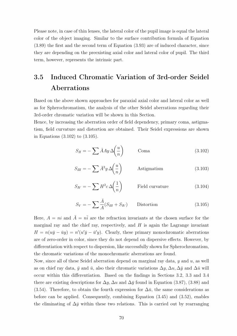
Please note, in case of thin lenses, the lateral color of the pupil image is equal the lateralcolor of the object imaging. Similar to the surface contribution formula of Equation(3.89) the first and the second term of Equation (3.93) are of induced character, sincethey are depending on the preexisting axial color and lateral color of pupil. The thirdterm, however, represents the intrinsic part.

3.5 Induced Chromatic Variation of 3rd-order Seidel

Aberrations

Based on the above shown approaches for paraxial axial color and lateral color as wellas for Spherochromatism, the analysis of the other Seidel aberrations regarding their3rd-order chromatic variation will be shown in this Section.Hence, by increasing the aberration order of field dependency, primary coma, astigma-tism, field curvature and distortion are obtained. Their Seidel expressions are shownin Equations (3.102) to (3.105).

𝑆𝐼𝐼 = −∑︁

𝐴𝐴𝑦 ∆

(︂𝑢

𝑛

)︂Coma (3.102)

𝑆𝐼𝐼𝐼 = −∑︁

𝐴2𝑦 ∆

(︂𝑢

𝑛

)︂Astigmatism (3.103)

𝑆𝐼𝑉 = −∑︁

𝐻2𝑐∆

(︂1

𝑛

)︂Field curvature (3.104)

𝑆𝑉 = −∑︁ 𝐴

𝐴(𝑆𝐼𝐼𝐼 + 𝑆𝐼𝑉 ) Distortion (3.105)

Here, 𝐴 = 𝑛𝑖 and 𝐴 = 𝑛�̄� are the refraction invariants at the chosen surface for themarginal ray and the chief ray, respectively, and 𝐻 is again the Lagrange invariant𝐻 = 𝑛(𝑢𝑦 − �̄�𝑦) = 𝑛′(𝑢′𝑦 − �̄�′𝑦). Clearly, these primary monochromatic aberrationsare of zero-order in color, since they do not depend on dispersive effects. However, bydifferentiation with respect to dispersion, like successfully shown for Spherochromatism,the chromatic variations of the monochromatic aberrations are found.Now, since all of these Seidel aberration depend on marginal ray data, 𝑦 and 𝑢, as wellas on chief ray data, 𝑦 and �̄�, also their chromatic variations ∆𝑦,∆𝑢,∆𝑦 and ∆�̄� willoccur within this differentiation. Based on the findings in Sections 3.2, 3.3 and 3.4there are existing descriptions for ∆𝑦,∆𝑢 and ∆𝑦 found in Equation (3.87), (3.88) and(3.54). Therefore, to obtain the fourth expression for ∆�̄�, the same considerations asbefore can be applied. Consequently, combining Equation (3.45) and (3.52), enablesthe eliminating of ∆𝑦 within these two relations. This is carried out by rearranging

70

the formulas for 𝐴𝑋𝐶𝑝,1𝑠𝑡 and 𝐿𝐴𝐶1𝑠𝑡 in the following way:

∆𝑦 =𝐴𝑋𝐶𝑝,1𝑠𝑡 + 𝑛𝑦∆�̄�

𝑛�̄�=

𝐿𝐴𝐶1𝑠𝑡 + 𝑛𝑦∆�̄�

𝑛𝑢(3.106)

Reordering this leads to the expression for the chromatic variation of the chief ray angle∆�̄�. The Equation is shown in (3.110), together with the prior derived expressions for∆𝑦,∆𝑢 and ∆𝑦. Please note, in order to simplify the following equations, the indicesare reduced by "1st", but still mean 1st-order color aberrations in any case.

∆𝑦 =𝑦𝐿𝐴𝐶𝑝 − 𝑦𝐴𝑋𝐶

𝐻(3.107)

∆𝑢 =𝑢𝐿𝐴𝐶𝑝 − �̄�𝐴𝑋𝐶

𝐻(3.108)

∆𝑦 =𝑦𝐴𝑋𝐶𝑝 − 𝑦𝐿𝐴𝐶

𝐻(3.109)

∆�̄� =𝑢𝐴𝑋𝐶𝑝 − �̄�𝐿𝐴𝐶

𝐻(3.110)

These four equations represent the main idea of the discussed approach within thisthesis. They explain how and why the paraxial marginal ray and chief ray varies inangle and in ray height on the way through the optical system, caused by the influenceof dispersion. The direct relation to prior summed paraxial color aberrations, 𝐴𝑋𝐶

and 𝐿𝐴𝐶, and pupil color aberrations, 𝐴𝑋𝐶𝑝 and 𝐿𝐴𝐶𝑝, found within this approach,now enables the calculation of the chromatic variations of all aberrations described bymarginal and chief ray data and additionally the differentiation of intrinsic and inducedparts.Considering these expressions for the four Seidel aberration Coma, Astigmatism, FieldCurvature and Distortion, the following final results are obtained after a differentia-tion with respect to dispersion. Here, 𝑐𝑆𝐼𝐼 , 𝑐𝑆𝐼𝐼𝐼 , 𝑐𝑆𝐼𝑉 and 𝑐𝑆𝑉 describe the chromaticvariations of 3rd-order Coma, Astigmatism, Field Curvature and Distortion, respec-tively. Again, the distinction between intrinsic and induced terms is possible by find-ing induced terms to depend on the prior summed up lower-order color aberrations𝐴𝑋𝐶,𝐴𝑋𝐶𝑝, 𝐿𝐴𝐶 and 𝐿𝐴𝐶𝑝.

71

𝑐𝑆𝐼𝐼 = 𝐴𝑋𝐶

(︂𝑐𝐻(𝑛 + 2𝑛′)

𝑛𝑛′ +3𝑛𝑦(𝑖′ + 𝑢)(̄𝑖𝑢′ − 𝑖�̄�)

𝐻+ 3𝑖(̄𝑖− 2�̄�) + 6̄𝑖′𝑢′ + 𝑢�̄�− 4𝑢′�̄�′

)︂+𝐴𝑋𝐶𝑝

𝑛𝑖𝑦(𝑖 + 𝑢′)(𝑢− 𝑢′)

𝐻

−(𝐿𝐴𝐶 − 3𝐿𝐴𝐶𝑝)(𝑢− 𝑢′)

(︂𝑛𝑖𝑦(𝑖 + 𝑢′)

𝐻+ (𝑖′ + 𝑢)

)︂−∆𝑛(𝑖𝑦 +

𝐻

𝑛)(︀𝑖′2 − 𝑖′(𝑢− 2𝑢′) + 𝑢(𝑢′ − 𝑢)

)︀+∆𝑛′𝑖′2𝑦(𝑖′ + 𝑢′) + ∆𝑛′𝑖′

𝐻

𝑛(𝑖′ − 𝑢 + 2𝑢′) + ∆𝑛′𝐻(𝑢− 𝑢′)(𝑢− 2𝑢′)

𝑛′ (3.111)

𝑐𝑆𝐼𝐼𝐼 =𝐴𝑋𝐶�̄�2 (𝐻 (𝑛′2 − 𝑛2) + 2𝑛𝑛′𝑦(𝑛′𝑢− 𝑛𝑢′))

𝐻𝑛′2

+𝐴𝑋𝐶𝑝(𝑢

′ − 𝑢)2𝑛�̄�𝑦(𝑖 + 𝑢′)

𝐻

+(𝐿𝐴𝐶 − 𝐿𝐴𝐶𝑝)(�̄�− �̄�′)2𝑛�̄�𝑦(𝑖 + 𝑢′)

𝐻

+∆𝑛�̄�2𝑦(𝑖𝑛′ − 𝑢(𝑛 + 2𝑛′) + 𝑢′(3𝑛 + 𝑛′))

𝑛′

+∆𝑛′̄𝑖2𝑦 (𝑛′(𝑢(𝑛 + 𝑛′) − 𝑖𝑛′) − 𝑢′ (2𝑛2 + 𝑛𝑛′ + 𝑛′2) + 𝑛2𝑢)

𝑛′2 (3.112)

𝑐𝑆𝐼𝑉 = − (𝐿𝐴𝐶 − 𝐿𝐴𝐶𝑝)2𝑐𝐻(𝑛− 𝑛′)

𝑛𝑛′ − ∆𝑛𝑐𝐻2(𝑛′ − 2𝑛)

𝑛2𝑛′ − ∆𝑛′ 𝑐𝐻2

𝑛′2 (3.113)

𝑐𝑆𝑉 = (𝐴𝑋𝐶�̄� + 3𝑖𝐿𝐴𝐶 − 𝑖𝐿𝐴𝐶𝑝)𝑦𝑛(̄𝑖 + �̄�′)(�̄�− �̄�′)

𝐻

+𝐴𝑋𝐶𝑝

(︂3𝑛𝑖𝑦(�̄�′(𝑖− 𝑢 + 𝑢′) − 𝑖�̄�)

𝐻− 𝑢(3�̄� + �̄�′) + 𝑢′(�̄� + 3�̄�′)

)︂+∆𝑛𝑖𝑦

(︀𝑖2 − 3̄𝑖�̄� + 4̄𝑖�̄�′ + �̄�2 − 4�̄��̄�′ + 3�̄�′2)︀

+∆𝑛2𝐻�̄�′(�̄�′2 + �̄�− �̄�)

𝑛

−∆𝑛′𝑦(︀𝑖𝑖2 + 4�̄�′(𝑖(̄𝑖− 2�̄�) + 𝑢�̄�) − 3𝑖𝑖�̄� + �̄�′2(5𝑖− 5𝑢 + 2𝑢′) + 3𝑖�̄�2 − 𝑢�̄�2

)︀+∆𝑛′𝐻(𝑛′�̄�′(−2̄𝑖 + �̄� + �̄�′) + 𝑛(�̄� + �̄�′)(�̄�− 2�̄�′))

𝑛𝑛′ (3.114)

72

4 Application of the New Theory

4.1 Classical Design Examples

In this Section some of the classical design examples for induced color aberrationsare investigated. All of them are kept very simple in design, since those are bestfor understanding the characteristics and possible influences of 2nd-order induced andintrinsic color aberrations. Particularly, the catadioptric system in 4.1.4 and the splitachromat in 4.1.5 are often-cited examples for induced color effects. But an exactanalytical analysis and therefore also a deeper understanding of them was missing.Here, the new surface contribution formulas, found in this thesis, can now be appliedand explain how these designs work.

4.1.1 8f-imaging System

As a first example a simple 8f-system composed of two lenses, each in a 4f-arrangement,is analyzed. Figure 4-1 illustrates the paraxial conditions for axial and lateral coloraberration.The primary wavelength is 𝜆 = 587 nm and a wavelength range from 𝜆1 = 486 nm to𝜆2 = 656 nm is assumed. The object height is 𝑦 = 1 mm. Note that the stop positionof the system is located after lens 2. Two cases shall be analyzed. Case (1) is describedby two, equiconvex lenses consisting of a 3 mm thick, low dispersive crown glass BK7,each with a focal length of 𝑓 ′ = 50 mm. In case (2) lens 1 now consists of SF6, ahigh dispersive flint glass and the center thickness of lens 2 is 12 mm. To analyzethese designs for intrinsic and induced color aberration, only a ray trace of the primarywavelength 𝜆 = 587 nm is required.

73

Figure 4-1: Example design composed of two lenses, each in a 4f- arrangement. (a) shows themarginal raytrace for two different wavelengths (dashed and dotted line), illus-trating the axial color parameters and (b) shows the chief raytrace of two differentwavelengths (solid and dotted line) illustrating the lateral color parameters.

Considering the equations for 1st- and 2nd-order axial color of Equation (3.18) twice,at first for 𝜆1 = 486 nm and secondly for 𝜆2 = 656 nm, and adding up these contri-butions, a differentiation between intrinsic and induced parts for a wavelength rangefrom 486 nm to 656 nm according to Table 4.1 and Table 4.2 is achieved.

Table 4.1: Axial color contributions for the example system for case (1). The wave-length range is 𝜆1 = 486 nm to 𝜆2 = 656 nm.

Surf.prior𝐴𝑋𝐶

1st𝐴𝑋𝐶

[mm]

2nd𝐴𝑋𝐶

[mm]

lensint

[mm]

lensind

[mm]

thickn.𝐴𝑋𝐶

[mm]

S1 0.000 1.449 −0.870 −0.034 0.000 0.0002

S2 0.004 1.459 0.836

S3 0.008

S4 0.008 1.508 −7.779 −0.036 −0.135 0.002

S5 0.012 1.518 7.609

S6 0.016

sum contrib. 5.934 −0.205 −0.070 −0.135 0.002

sum 1st+2nd 5.729

sum system 5.747

74

Table 4.2: Axial color contributions for the example system for case (2). The wave-length range is 𝜆1 = 486 nm to 𝜆2 = 656 nm.

Surf.prior𝐴𝑋𝐶

1st𝐴𝑋𝐶

[mm]

2nd𝐴𝑋𝐶

[mm]

lensint

[mm]

lensind

[mm]

thickn.𝐴𝑋𝐶

[mm]

S1 0.000 3.261 −6.515 −0.217 0.000 0.001

S2 0.010 3.284 6.298

S3 0.020

S4 0.020 1.368 −7.369 −0.031 −0.548 0.025

S5 0.024 1.397 6.790

S6 0.028

sum contrib. 9.310 −0.795 −0.248 −0.548 0.026

sum 1st+2nd 8.515

sum system 8.658

Assuming then the same considerations for lateral color (Equation (3.56)) and takingadditionally the rear sided stop position into account, the results of Table 4.3 and Table4.4 are obtained.

Table 4.3: Lateral color contributions for the example system for case (1). Thewavelength range is 𝜆1 = 486 nm to 𝜆2 = 656 nm.

Surf.prior

𝑖𝐴𝑋𝐶𝑝

10−3

prior�̄�𝐿𝐴𝐶

10−3

1st𝐿𝐴𝐶

[mm]

2nd𝐿𝐴𝐶

[mm]

lensint

[mm]

lensind

[mm]

thickn.𝐿𝐴𝐶

[µm]

S1 −0.113 0.000 −27.53 0.499 0.003 0.888 0.003

S2 0.033 −0.033 −17.77 0.392

S3 0.003 −0.013

S4 0.009 0.008 1.72 0.001 0.000 −0.172 0.005

S5 −0.005 −0.034 11.67 −0.173

S6 0.000 −0.023

sum contrib. −31.92 0.719 0.003 0.715 0.008

sum 1st+2nd −31.20

sum system −31.23

75

Table 4.4: Lateral color contributions for the example system for case (2). Thewavelength range is 𝜆1 = 486 nm to 𝜆2 = 656 nm.

Surf.prior

𝑖𝐴𝑋𝐶𝑝

10−3

prior�̄�𝐿𝐴𝐶

10−3

1st𝐿𝐴𝐶

[mm]

2nd𝐿𝐴𝐶

[mm]

lensint

[mm]

lensind

[mm]

thickn.𝐿𝐴𝐶

[µm]

S1 −0.191 0.000 −67.05 3.086 0.019 5.189 0.018

S2 0.041 −0.046 −36.15 2.122

S3 0.004 −0.026

S4 0.011 0.033 2.86 −0.096 −0.001 −0.577 0.055

S5 −0.006 −0.086 11.49 −0.483

S6 0.000 −0.072

sum contrib. −88.85 4.63 0.02 4.61 0.07

sum 1st+2nd −84.23

sum system −84.68

Comparing case (1) and case (2) shows clearly the influence of preexisting 1st-ordercolor aberrations, expressed by the prior 1st-order parameters 𝐴𝑋𝐶,𝐴𝑋𝐶𝑝 and 𝐴𝑋𝐶𝑝

according to Equation (3.25), (3.65) and (3.66). In case (1), due to the low dispersiveBK7 lens, small 1st- order axial color aberrations are summed up until the light hitslens 2. Hence, the induced contributions equal only 2.4% of the overall sum for axialcolor of the 8f-system. In contrast to this, in case (2) the high dispersive flint glassSF6 produces large 1st-order axial color aberrations ∆𝑠1 at the intermediate imagein front of lens 2(Figure 4-1). This induces larger 2nd-order terms at the second lenscompared to case (1). Here, they reach up to 6.5% of the overall aberration. It shouldalso be noted that the individual 2nd-order surface contributions are partly of sameorder of magnitude as the 1st-order ones and also at some points larger. The lenscontributions, however, in all cases show the expected lower order of magnitude. Thesame basic conclusions as for axial color are also true for lateral color. Since theinduced lateral color aberrations show a linear dependency on (𝑖𝐴𝑋𝐶𝑝,1𝑠𝑡 − �̄�𝐿𝐴𝐶1𝑠𝑡),the 1st-order parameters 𝑖𝐴𝑋𝐶𝑝 and �̄�𝐿𝐴𝐶 are plotted in Table 4.3 and Table 4.4 asreference. Here, additionally the influence of the rear sided stop location at surfaceS6 has to be considered. Hence, in Table 4.3 and Table 4.4 non-zero off-set values forprior 𝑖𝐴𝑋𝐶𝑝,1𝑠𝑡 are present, which then sum up surface by surface and become zero atsurface S6, since the real stop position is located here. These non-zero off-set conditionsare also the reason for the large induced contributions of lens 1 compared to lens 2. Inthis regard, Table 4.3 shows an eight times larger induced contribution of lens 1 andTable 4.4 illustrates even a factor of ten between lens 1 and 2.Additionally the increased thickness of lens 2 in case (2) leads to a rise of thickness

76

depending terms by a factor of twelve for 2nd-order axial color and by a factor of elevenfor 2nd-order lateral color compared to case (1).In summary, although this is a very simple design example composed of only twolenses, very large 2nd-order effects dominated by the induced parts in both cases andfor both color aberration are present. The reason for this effect can be found in thewidely separated lenses. Hence, the introduced color aberration of lens 1 leads tolarge differences in ray angles and ray heights at the second lens for the differentwavelengths. Consequently, in optical systems like this, where single, non achromizedlenses are widely separated from each other, induced color aberration parts can reachup to 9.3% or even more of the overall aberration (Table 4.3 and Table 4.2 ). Withoutconsidering those contributions here, a 1st-order prediction would show an error of7.5% compared to the real design value. But by considering the 2nd-order effects theerror reduces to only 1.6%.

4.1.2 Thick Meniscus

As a second example, a single meniscus lens, focusing light from infinity, is analyzedfor axial color. Figure 4-2 illustrates this lens setup.

Figure 4-2: Thick meniscus lens with same radii of 𝑅 = 15mm and a thickness of𝑡 = 10mm.

Both radii of the lens are supposed to have the same value of 𝑅 = 1/𝑐1 = 1/𝑐2 = 15 mm.The center thickness is 10 mm. Assuming F2 as a glass material for the meniscus lens,the resulting sums of intrinsic and induced surface contributions are shown in Table4.5.Note, for such a meniscus lens the thin lens formula for 2nd-order axial color contri-butions by Nobis [Nob14] is no longer valid, since the thin lens approach would resultin a 2nd-order contribution of zero for the meniscus lens. Instead of that, the newsurface approach applied in Table 4.5, shows the first surface already inducing a rele-vant amount of 2nd-order axial color at the second surface. In combination with thethickness of the lens, a significant amount of 2nd-order intrinsic and induced effectsare present.

77

Table 4.5: Induced and intrinsic axial color contributions of a meniscus lens for awavelength range from 486 nm (F-line) to 587 nm (d-line).

Surf. R[mm]

t[mm]

glass 1st𝐴𝑋𝐶[mm]

2nd𝐴𝑋𝐶[mm]

surf.int

[mm]

surf.ind

[mm]

STOP 10 0 0 0 0S2 15 10 F2 4.455 −0.087 −0.087 0S3 15 70.62 −1.946 0.016 −0.054 0.069

sum contrib. 2.508 −0.071 −0.140 0.069sum 1st+2nd 2.437sum system 2.439

4.1.3 Schupmann Achromat

The third example shows an one-glass dialyte lens, presented in Figure 4-3. Dialytesenable color correction at a virtual image plane with two widely air spaced lenses,consisting of the same glass material [Kin12]. Figure 4-3(a) shows this classical two-lens setup.

Figure 4-3: (a) Schupmann achromatic design, where a positive lens with 𝑓 ′𝐿1 and negative

lens with 𝑓 ′𝐿2 = −𝑓 ′

𝐿1 are set up together, separated by an airspace of 𝑑 = 2𝑓 ′𝐿1.

(b) Schupmann design improved by a third lens with 𝑓 ′𝐿3 = 1/2𝑓 ′

𝐿1, positionedexactly at the intermediate image between the two lenses.

In case of the Schupmann Achromat, a positive lens L1 with a focal length 𝑓 ′𝐿1 and a

negative lens L2 with a focal length of 𝑓 ′𝐿2 = −𝑓 ′

𝐿1 are set up together separated by anairspace 𝑑 = 2𝑓 ′

𝐿11. According to 1st-order theory, such a design is perfectly correctedfor axial color. This is a result of the same dispersive behavior of both lenses, sincethey are made of the same glass. The 1st-order axial color introduced by lens L1 isexactly canceled out by the 1st-order axial color contribution of lens L2, as they have

78

equal but opposite power and are operating at identical marginal ray heights. However,for secondary color, a significant amount of color aberration is left, which cannot beexplained with this 1st-order approach. Nobis showed in [Nob14] how 2nd-order coloraberration, including induced aberration parts, leads to this amount of secondary color.Furthermore, he also proved with his approach that an additional third lens L3, with𝑓 ′𝐿3 = 1/2𝑓 ′

𝐿1 positioned exactly at the intermediate image between the two lenses, canalmost perfectly correct the secondary color of the system by introducing additionalinduced axial color amounts. This design setup is shown in Figure 4-3(b). Now, Figure4-4 gives the longitudinal aberration plot for the classical two- lenses and the improvedthree-lenses Schupmann design, assuming 𝑓 ′

𝐿1 = −𝑓 ′𝐿2 = 2𝑓 ′

𝐿3 = 50 mm and N-BK7 tobe the glass material. The entrance pupil diameter is chosen to be 7 mm and the lensesare assumed to be thin lenses with either a plano-convex or plano-concave shape.

Figure 4-4: Longitudinal aberration plots for (a) the two-lenses N-BK7 Schupmann designand (b) the same Schupmann design improved by a third N-BK7 thin lens withpositioned exactly at the intermediate image between the two lenses.

These longitudinal aberration plots clearly show that not only secondary color is cor-rected, but also spherochromatism is completely vanishing by inserting the additionalthird lens.Now, according to the thin lens formula derived in Equation (3.93), the total sphe-rochromatism amount 𝐺𝐿

𝑡𝑜𝑡 for the classical two-lens Schupmann Achromat is obtainedby the sum of both thin lens contributions 𝐺𝐿1 and 𝐺𝐿2:

𝐺𝐿𝑡𝑜𝑡 = 𝐺𝐿1 + 𝐺𝐿2 (4.1)

Considering the induced terms of 𝐺𝐿1 to be zero, since no prior axial and lateral colorwas summed up previously, 𝐺𝐿

𝑡𝑜𝑡 is determined by adding up the intrinsic part 𝐺𝐿1𝑖𝑛𝑡

of lens L1 and the induced as well as the intrinsic part of lens L2, 𝐺𝐿2𝑖𝑛𝑡 and 𝐺𝐿2

𝑖𝑛𝑑

79

respectively:

𝐺𝐿𝑡𝑜𝑡 = 𝐺𝐿1

𝑖𝑛𝑡 + 𝐺𝐿2𝑖𝑛𝑡 + 𝐺𝐿2

𝑖𝑛𝑑 (4.2)

Assuming now 𝜆1 = 546 nm to be the primary wavelength and 𝜆2 = 480 nm as thesecond wavelength, Table 4.6 represents those results.

Table 4.6: 𝐺𝐿 coefficients of the two-lens Schupmann design for the prior summedup 1st-order color aberrations 𝐴𝑋𝐶𝐿 and 𝐿𝐴𝐶𝐿

𝑝 and the intrinsic andinduced parts of 𝐺𝐿

Lens 𝑦

[mm]

𝑦

[mm]

prior𝐴𝑋𝐶𝐿

10−4

[mm]

prior𝐿𝐴𝐶𝐿

𝑝

10−4

[mm]

𝐺𝐿

10−4

[mm]

int𝐺𝐿

10−4

[mm]

ind𝐺𝐿

10−4

[mm]

L1 3.5 0 0 0 −0.03 −0.03 0L2 3.5 2 9.7 0 0.45 0.11 0.34

sum 0.42 0.08 0.34

Similar to Nobis’ axial color study of the Schupmann design [Nob15], the analysis,shown in Table 4.6, indicates a dominating amount of induced aberration parts forspherochromatism also. Lens L2 introduces more than 80% of the total spherochroma-tism amount by its induced aberration parts. Since the prior summed up lateral colorof the imaged stop is equal to zero for that lens, the whole induced amount is causedby the 1st-order axial color of lens L1.If now the third lens L3 is insert into the system, its spherochromatism contribution,represented by 𝐺𝐿3

𝑖𝑛𝑡 and 𝐺𝐿3𝑖𝑛𝑑, has to be added to the total spherochromatism amount

𝐺𝐿𝑡𝑜𝑡 :

𝐺𝐿𝑡𝑜𝑡 = 𝐺𝐿1

𝑖𝑛𝑡 + 𝐺𝐿2𝑖𝑛𝑡 + 𝐺𝐿2

𝑖𝑛𝑑 + 𝐺𝐿3𝑖𝑛𝑡 + 𝐺𝐿3

𝑖𝑛𝑑 (4.3)

Here, the position of lens L3 at the intermediate image, where the marginal ray heighty is zero, causes some special conditions. First of all, according to Equation (3.93)this position leads to a zero spherochromatism contribution of lens L3 for the inducedas well as for the intrinsic case, since in all terms of Equation (3.93) the marginal rayheight y occurs as a constant factor. Hence, the terms 𝐺𝐿3

𝑖𝑛𝑡 and 𝐺𝐿3𝑖𝑛𝑑 of Equation (4.3)

vanishes and the total amount of spherochromatism in the three-lens system again onlydepends on the contributions of L1 and L2.Furthermore, the special position of L3 enables also the same marginal ray propagationlike for the two-lens design. For this reason, the ray heights and ray angles at lens L1and lens L2 are still the same as before, which causes a conservation of both intrinsic

80

contributions of L1 and L2. Therefore, the total intrinsic sum of the two-lens design iskept and its value of 0.08 × 10−4 mm can be insert into Equation (4.3):

𝐺𝐿𝑡𝑜𝑡 = 0.08 × 10−4 mm + 𝐺𝐿2

𝑖𝑛𝑑 (4.4)

Now, Equation (4.4) clearly shows that only the induced parts of lens L2 are left forcorrecting the system’s spherochromatism. These two induced terms are shown inEquation (4.5).

𝐺𝐿2𝑖𝑛𝑑 = (𝑦𝐴𝑋𝐶𝐿2

1𝑠𝑡 − 𝑦𝐿𝐴𝐶𝐿2𝑝,1𝑠𝑡)

4𝑦𝐹

𝐻𝑛𝐿

𝛾1 + 𝐴𝑋𝐶𝐿21𝑠𝑡

𝑦𝐹

𝑛𝐿

𝛾2 (4.5)

Due to the fact that the marginal ray height y at the position of L3 equals to zero andconsidering then Equation (3.100) and (3.101) for the prior summed up 1st-order coloraberrations, neither an additional axial color contribution nor an additional lateralcolor contribution of lens L3 is introduced to the system. With that, the prior summedup color aberrations in front of lens L2 are also maintained and still show the values of𝐴𝑋𝐶𝐿2

1𝑠𝑡 = 9.7×10−4 mm and 𝐿𝐴𝐶𝐿2𝑝,1𝑠𝑡 = 0 mm like for the two-lens chase. Considering

all of these simplifications, the only left parameter, which is changed by inserting thethird lens L3, is the chief ray height 𝑦𝐿2 at lens L2. By inserting all of the maintainedvalues into Equation (4.5), the following simple relation is gained.

𝐺𝐿2𝑖𝑛𝑑 = − 0.08 × 10−4 mm + 0.21 × 10−4 mm 𝑦𝐿2 (4.6)

Finally, it is easy to see that the remaining overall spherochromatism 𝐺𝐿𝑡𝑜𝑡 of the three-

lens system, shown in Equation (4.4), can only be corrected completely, if the chief rayheight 𝑦𝐿2 at lens L2 becomes zero. Since this condition is perfectly fulfilled, if the focallength of L3 is exactly 𝑓 ′

𝐿3 = 1/2𝑓 ′𝐿1, for the first time the above shown derivation can

prove analytical that not only secondary color is corrected, but also spherochromatismis completely vanishing by inserting the additional third lens with half of the focallength of L1 and L2 at the intermediate image. (Figure 4-3 and 4-4)

4.1.4 Catadioptric System

Since the probably most impressive example on induced color aberrations is the simpledesign, focusing light, coming from infinity, by two elements, a positive spherical lensand a collecting spherical mirror, this kind of system dealing with spherochromatismis now investigated. The design is illustrated in Figure 4-5. Here, the biconvex lens is

81

made of the high dispersive flint glass NSF6 with an center thickness of 2 mm and radiiof 𝑅1 = −𝑅2 = 50 mm. The distance to the mirror equals 16mm and the mirror’s radiusis 𝑅𝑀 = −30 mm. A stop is placed 6 mm in front of the lens and shows a diameter of10 mm. Furthermore, the light is coming from infinity within a field of view of ±1 deg.For the described case, the primary wavelength is chosen to be 𝜆1 = 587 nm with asecond wavelength, which is 𝜆2 = 656 nm.

Figure 4-5: Thick meniscus lens with same radii of 𝑅 = 15mm and a thickness of𝑡 = 10mm.

Table 4.7 summarizes the Seidel results for the spherical aberration coefficient 𝑆𝐼 ,gained by two single paraxial ray traces for 𝜆1 and 𝜆2. Additionally, the resultingdifferences are calculated and plotted in the third column. Therefore, the first threecolumns describe, how spherochromatism contributions where identified in the past.Now, the fourth column represents the 3rd-order spherochromatism values 𝐺 obtainedby Equation (3.89) of this thesis. Hence, for this values, only the ray trace data of theprimary wavelength were used and no additional raytrace for the second wavelengthwas needed. Comparing the results, shows the very high accuracy of 𝐺. Please note,the only reason for the remaining error are the small differences in ray heights and rayangles caused by higher order effects of axial and lateral color.

Table 4.7: Seidel wavefront aberration coefficient 𝑆𝐼 by two single ray traces and thecomparison to the spherochromatic coefficient 𝐺.

Surf. 𝑆𝐼,𝜆1

[mm]𝑆𝐼,𝜆2

[mm]𝑆𝐼,𝜆2 − 𝑆𝐼,𝜆1

[mm]G

[mm]

S1 0 0 0 0S2 −0.001 24 −0.001 23 0.000 01 0.000 01S3 −0.044 03 −0.042 86 0.001 17 0.001 18S4 −0.021 01 −0.021 39 −0.000 38 −0.000 38

sum −0.066 28 −0.065 49 0.000 79 0.000 80

Table 4.8 and Table 4.9 now illustrate the main advantage of Equation (3.89). Besidesthe above shown benefit of 𝐺 by following the basic idea of Seidel’s approach, as it

82

ensures the calculation by tracing only the paraxial rays for the primary wavelength,this formula furthermore allows the differentiation of intrinsic and induced parts. Theseparts considering Equation (3.89) are shown in Table 4.8. In addition, also the priorsummed up amounts of 𝐴𝑋𝐶1𝑠𝑡 and 𝐿𝐴𝐶𝑝,1𝑠𝑡 in front of the different surfaces, accordingto Equation (3.94) and (3.94), are given. For this design example, each of the threesystem surfaces show a different distribution of intrinsic and induced parts. The firstsurface of the lens does not exhibit any induced spherochromatism contribution. Thewhole amount is of intrinsic character. This is caused since it represents the first opticalsurface of the system, where no 1st-order color aberrations like 𝐴𝑋𝐶1𝑠𝑡 and 𝐿𝐴𝐶𝑝,1𝑠𝑡

could sum up before. Hence, the two terms of Equation (3.89), depending on this,also become zero and only the intrinsic terms, depending on the dispersive behaviorof the surface are left. In contrast to this, surface S3 shows both, an intrinsic part ofspherochromatism and an induced part. Here, the prior axial color and lateral color ofthe imaged stop, introduced by surface S2, causes the induced amount of S3. Moreover,also the intrinsic parts are present, since surface S3 is again a lens surface suffering fromdispersion. Finally, the mirror surface S4 is the most interesting one. Table 4.7 alreadyshowed that S4 is suffering from a chromatic variation of spherical aberration, althoughthis is the mirror surface of the system. Due to the fact that mirrors inherently do nothave dispersive characteristics, the input of the mirror surface S4 on spherochromatismwas not explainable by any common used 3rd-order theory before. Table 4.8 now givesthe reason for this. Since the lens is the only dispersive element in the system, themirror’s spherochromatic behavior is completely caused in front of it by the lens’ priorintroduced 1st-order lateral color of the imaged stop as well as its axial color aberration.No intrinsic parts are present for S4.

Table 4.8: Wavefront aberration coefficients of the mirror design example for theprior summed up chromatic aberrations 𝐴𝑋𝐶1𝑠𝑡 and 𝐿𝐴𝐶𝑝,1𝑠𝑡 and theintrinsic and induced parts of 𝐺.

Surf.prior𝐴𝑋𝐶[mm]

prior𝐿𝐴𝐶𝑝

[mm]

total𝐺

[mm]

int𝐺

[mm]

ind𝐺

[mm]

STOP 0 0 0 0 0S2 0 0 0.000 01 0.000 01 0S3 −0.0025 −0.000 05 0.001 18 0.000 91 0.000 27S4 −0.0089 −0.000 21 −0.000 38 0 −0.000 38

sum 0.000 80 0.000 91 −0.000 11

As an addition, Table 4.9 shows the equivalent longitudinal values of the spherochro-matism contributions. Here, the adapted conversion relation of Equation (3.96) wasapplied. Please note, for the marginal ray angle 𝑢′

𝑆4𝜆2of the second wavelength, the

83

calculation according to Equation (3.94) and (3.95), also has to be adapted individu-ally for identifying the intrinsic and induced parts. For example, when determining theintrinsic amounts of 𝐺, the 𝐴𝑋𝐶1𝑠𝑡 and 𝐿𝐴𝐶𝑝,1𝑠𝑡 contributions in front of the surfacehave to be neglected, when calculating the image space sum of 𝐴𝑋𝐶1𝑠𝑡 and 𝐿𝐴𝐶𝑝,1𝑠𝑡

by (3.94) and (3.95), since by definition of the intrinsic parts, all of the color contribu-tions in front of the surface are ignored. Following then the characteristics of inducedaberrations, the difference between the total longitudinal amount at the image andthe intrinsic longitudinal amount at the image equals the longitudinal induced sum ofspherochromatism in image space.To finally compare the spherochromatism results to the exact longitudinal value of0.004 58 mm, determined by a real raytrace, Table 4.9 additionally shows the differencebetween the 3rd-order approximation and the exact value in the last row. Here, againthe results are in very good agreement with the actual ray trace results. The mainreason for the remaining error of ca. 10% is the 3rd-order approximation of the sphericalaberration. The exact value of spherochromatism includes terms of higher-order, whichare not considered here. Therefore, for other design examples, where also higher-orderspherical aberration is present, such errors may become larger. But for systems withsmall 5th-order contributions on spherical aberration, the accuracy is as high as shownhere.

Table 4.9: Conversation of Seidel’s spherical aberration coefficients and of the sphe-rochromatism coefficient 𝐺 into longitudinal aberrations 𝑆𝑃𝐻 and 𝐺𝐴

Surf. 𝑆𝑃𝐻𝜆2 − 𝑆𝑃𝐻𝜆1

[mm]

total𝐺𝐴[mm]

int𝐺𝐴[mm]

ind𝐺𝐴[mm]

STOP 0 0 0 0S2 0.000 01 0.000 01 0.000 01 0S3 0.006 04 0.006 09 0.004 64 0.001 45S4 −0.001 77 −0.001 77 0 −0.001 77

sum 0.004 28 0.004 33 0.004 65 −0.000 32error −0.000 31 0.000 25

4.1.5 Split Achromat

The last example to gain a deeper analytical understanding for a simple, but still lessanalytically discussed lens system is the split achromat.Figure 4-6 (a) shows a classical achromatic design of two lenses made of NBK7 (crownglass) and NSF5 (flint glass). The focal length is set to be 𝑓 ′ = 100 mm and theentrance pupil diameter is 20 mm. In literature, the example of a split achromat,exhibited in Figure 4-6 (b), is often showed for correcting spherochromatism, since

84

the main aberration left for a classical, unsplit achromat is the chromatic variation ofspherical aberration [KT02] [Kin12]. The longitudinal aberration plot in Figure 4-7(a) demonstrates this conditions. Here, spherical aberration of the primary wavelength𝜆2 = 587 nm as well as axial color between 𝜆1 = 486 nm and 𝜆3 = 656 nm is cor-rected. But for zonal and maximum pupil height spherical aberration of those twoouter wavelengths separate widely and causes still a large on axial spot size. However,the longitudinal aberration plot of the split achromat, shown in 4-7 (b), indicates anadditional corrected spherochromatism for the maximal pupil height.The reason for this are the different numbers of degrees of freedom within the systems.By assuming thin lenses and if the glass combination of the achromat is fixed, theunsplit achromat offers only three degrees of freedom. Those are the three radii of thesystem. Requiring a certain focal length of 𝑓 ′ = 100 mm, only two additional conditionscan be solved. Hence, in case of the achromat shown in 4-6 (a), these conditions are thecorrection of spherical aberration 𝑆𝑃𝐻 of the primary wavelength and the correctionof axial color 𝐴𝑋𝐶.

Figure 4-6: (a) a classical unsplit achromat and (b) a split achromat with a air space betweenthe lenses.

Figure 4-7: Longitudinal aberration plots for (a) the classical unsplit achromat and (b) thesplit achromat with a air space between the lenses. The first, positive lens is madeof NBK7 and the second, negative lens of NSF5.

In case of spherical aberration, the longitudinal aberration plot also illustrates the

85

existence and the need of higher order spherical aberration for correction. This canbe proven, since its longitudinal dependency on pupil height is not only of lowest,quadratic character. For large pupil heights, higher order spherical aberration termsenable the reversal of the graph and therefore the correction of spherical aberration formaximum pupil height. Consequently, only the sum of 3rd- and higher-order sphericalaberration leads to a corrected overall spherical aberration. In literature, Buchdahl[Buc54] and Rimmer [Rim63] derived a 5th-order surface contributions for monochro-matic aberrations, assuming the same ray based approach like Seidel. Here, 5th-orderspherical aberration is named 𝐵5 and will be applied here. Its explicit formula givenby Buchdahl and Rimmer can be found in the appendix.Therefore, regarding the unsplit achromat, the three condition, which can be solved,are:

𝑓 ′ = 100𝑚𝑚 (4.7)

𝐴𝑋𝐶 =𝑆3∑︁𝑆1

𝐶1 =𝑆3∑︁𝑆1

𝑛𝑖𝑦

(︂∆𝑛′

𝑛′ − ∆𝑛

𝑛

)︂= 0 (4.8)

𝑆𝑃𝐻 =𝑆3∑︁𝑆1

𝑆𝐼 + 𝐵5 =𝑆3∑︁𝑆1

𝑛2𝑖2𝑦 ∆

(︂𝑢

𝑛

)︂+

𝑆3∑︁𝑆1

𝐵5 = 0 (4.9)

By applying paraxial relations (Section 2.1) and solving this system of equations forthe given glass combination of NBK7 and NSF5, an achromat with the following radii𝑅1, 𝑅2 and 𝑅3, axial color as well as spherical aberration contributions is obtained.(Table 4.10)

Table 4.10: Numerical solution for three variable radii 𝑅1, 𝑅2 and 𝑅3 of the unsplitachromat. The Seidel contributions for axial color 𝐴𝑋𝐶 and 3rd-orderspherical aberration 𝑆𝐼 as well as the Buchdahl-Rimmer 5th-order con-tributions 𝐵5 are given.

Surf. 𝑅[mm] Glass 𝐴𝑋𝐶

[mm]𝑆1

[mm]𝐵5

[mm]

S1 54.864 NBK7 −0.009 68 0.013 60 −0.000 26S2 −48.365 NSF5 0.029 20 −0.031 26 0.002 11S3 −176.850 −0.019 52 0.019 08 −0.000 43

sum 0.000 0.0142 −0.0142

Here, the perfect correction of 1st-order axial color 𝐴𝑋𝐶 and spherical aberration𝑆𝑃𝐻, including 3rd-order and 5th-order contributions, are shown.Comparing those results with optimized values by a damped least squares algorithm,the exact radii would be 𝑅1 = 54.480 mm, 𝑅2 = −48.668 mm and 𝑅3 = −180.963 mm

to fulfill the conditions of 𝑓 ′ = 100 mm, a corrected axial color and a corrected spherical

86

aberration. Compared to the values of the Table 4.10, there are only small differencesleft, which verifies the above described approach. Furthermore, these differences indi-cates an additional, but small presents of even higher spherical aberration orders.Now, due to the new surface resolved spherochromatism formula found in Section 3.4,the same approach can be followed for the first time also for a split achromat. Theadvantage of the split achromat design is the larger number of degrees of freedom byintroducing the additional air space. Hence, two more variables within the system aregenerated, the size of the air space and the extra fourth radius. Regarding the addi-tional correction of spherochromatism 𝐺, only one extra variable is required. A secondone could be assumed to minimize also zonal spherical aberration by introducing evenhigher order spherical aberration terms. But this will not be investigated here. Con-sequently, one radius given from the unsplit achromat can be fixed and the remainingthree radii as well as the air space are set to be variable. Therefore, in case of thesplit achromat, these four conditions, now including spherochromatism 𝐺, have to besolved:

𝑓 ′ = 100𝑚𝑚 (4.10)

𝐴𝑋𝐶 =𝑆3∑︁𝑆1

𝐶1 =𝑆3∑︁𝑆1

𝑛𝑖𝑦

(︂∆𝑛′

𝑛′ − ∆𝑛

𝑛

)︂= 0 (4.11)

𝑆𝑃𝐻 =𝑆3∑︁𝑆1

𝑆𝐼 + 𝐵5 =𝑆3∑︁𝑆1

𝑛2𝑖2𝑦 ∆

(︂𝑢

𝑛

)︂+

𝑆3∑︁𝑆1

𝐵5 = 0 (4.12)

𝐺 =𝑆3∑︁𝑆1

(𝑦𝐴𝑋𝐶1𝑠𝑡 − 𝑦𝐿𝐴𝐶𝑝,1𝑠𝑡)4𝑖𝑛

𝐻(𝑢− 𝑢′)(𝑖 + 𝑢′)

− 𝐴𝑋𝐶1𝑠𝑡(𝑢− 𝑢′)(𝑢′ − 3𝑢− 4𝑖′)

− ∆𝑛𝑖𝑦(︀(𝑢′ − 𝑢)2 − (𝑖′ + 𝑢′)2 + 𝑢(𝑖′ + 𝑢′)

)︀− ∆𝑛′𝑖′2𝑦(𝑖′ + 𝑢′) = 0 (4.13)

The numerical results, found by solving this system of four equations assuming thegiven glass combination of NBK7 and NSF5, can be found in Table 4.11. The fourvariables are 𝑅2, 𝑅3, 𝑅4 and the size of air space t in between both lenses. 𝑅1 is keptas 𝑅1 = 54.480 mm.For the first time, the results shown in Table 4.11 analytically confirm the well-knownand often discussed possibility to correct also Spherochromatism, besides axial colorand spherical aberration, by applying an additional air space between both lenses ofan achromat.Although, the longitudinal plots of Figure 4-7(b) may constitute the need of considera-

87

tions for even higher-order Spherochromatism, again a comparison to optimized valuesby a damped least squares algorithm approves the here applied approach. The exactradii found by this are 𝑅1 = 54.480 mm, 𝑅2 = −38.972 mm, 𝑅3 = −32.522 mm as wellas 𝑅4 = −103.775 mm and the optimized air space is 𝑡 = 4.505 mm. The differencesto the values of Table 4.11 are still small, which indicates a present but still almostnegligible influence of higher orders. Hence, the main correction effects are exceptedto be caused by 3rd-order spherochromatism.

Table 4.11: Numerical solution for three variable radii 𝑅2, 𝑅3, 𝑅4 and a variableair space thickness t of the split achromat. The Seidel contribution foraxial color 𝐴𝑋𝐶 and 3rd-order spherical aberration 𝑆𝐼 as well as theBuchdahl-Rimmer 5th-order contributions 𝐵5 and the Spherochroma-tism contributions 𝐺 are given.

S 𝑅[mm]

𝑡[mm] Glass 𝐴𝑋𝐶

[mm]𝑆𝐼

[mm]𝐵5

[mm]𝐺

[mm]

S1 54.48 0 NBK7 −0.0098 0.0139 −0.0003 0.0001S2 −36.06 5.612 −0.0274 0.5234 −0.0948 0.0171S3 −28.50 0 NSF5 0.0586 −0.5758 0.0861 −0.0171S4 −87.93 100 −0.0215 0.0300 0.0006 0.0001

sum 0.000 −0.0085 −0.0084 0.000

Furthermore, the new surface contributions also enables an deeper understanding, whyand how the correction is possible. The main contributions on spherochromatismare clearly found at both inner surfaces, S2 and S3. Here, S3 exactly cancels out thecontribution of S2. Furthermore, these are those two radii, which are directly in contactwith the additional variable air space between the two lenses. The first and the lastsurface, S1 and S4, almost do not contribute at all.Following that finding, a complementary investigation for the other three design ver-sions, where 𝑅2, 𝑅3 and 𝑅4 are kept, showed that solutions also can be found for afixed 𝑅2 and 𝑅4, but by fixing 𝑅3 there is no existing solution solving the system ofthe four equations. Therefore, to complete the understanding on why and how the cor-rection of spherochromatism works within this design, Table 4.12 shows the separationof induced and intrinsic spherochromatism contributions for the same case like Table4.11.Emphasizing the dominating role of S3, the analysis of Table 4.12 also shows the in-duced part to be the main contributor for surface S3. Hence, to understand how theadditional air space can correct spherochromatism, the three variable radii R2, R3 andR4 are again assumed to solve the conditions of the focal length to be 𝑓 ′ = 100 mm,a corrected axial color and a corrected spherical aberration like for the unsplit case.Now, the thickness 𝑡 of the air space is left to enable the correction of spherochroma-

88

tism 𝐺. Since this is only possible due to induced effects of surface S3, the optimumthickness 𝑡 of the airspace is strongly connected to the prior introduced lower ordercolor aberration of the system before and the radius 𝑅3 of surface S3. Following thatand considering the results of Table 4.12, the single, exact solution for 𝑡 only is found,if the induced part of S3, caused by the prior introduced color aberration of the firstlens, plus the intrinsic part of S3, caused by the radius 𝑅3, exactly cancels out thespherochromatism contributions introduced by the first lens.

Table 4.12: Numerical solution for three variable radii 𝑅2, 𝑅3, 𝑅4 and a variable airspace thickness t of the split achromat. The spherochromatism contri-butions 𝐺 and its intrinsic as well as its induced parts are given.

S 𝑅[mm]

𝑡[mm]

Glass 𝐺[mm]

int𝐺

[mm]

ind𝐺

[mm]

S1 54.80 0 NBK7 0.0001 0.0001 0.0000S2 −36.06 5.612 0.0171 0.0136 0.0035S3 −28.50 0 NSF5 −0.0171 −0.0064 −0.0107S4 −87.93 100 0.0001 0.0016 −0.0015

sum 0.000 0.009 −0.009

4.2 Complex Design Example - A Microscope Objec-

tive Lens

Compared to the classical and to same extend academic design examples of Section 4.1,now a more complex microscope objective lens is investigated. Although the simpledesign examples are best for understanding the characteristics and possible influenceof 2nd-order induced and intrinsic color aberrations, a more complex design exampleshows a higher relevance for the practical work of an optical designer. Here, very oftensystems of many lenses within compact arrangements and a multitude of possible glasscombinations are present. Especially for those systems, a surface resolved analysiscan be the key method to find out the inner workings of the optical system and tounderstand why the present left aberrations arise at the final image plane.

4.2.1 Design Specifications

Microscope objectives represent a special kind of optical systems. They are essentiallydiffraction-limited optical devices with small object fields, but extremely high numer-ical apertures in object space. Therefore, microscope lenses are usually characterized

89

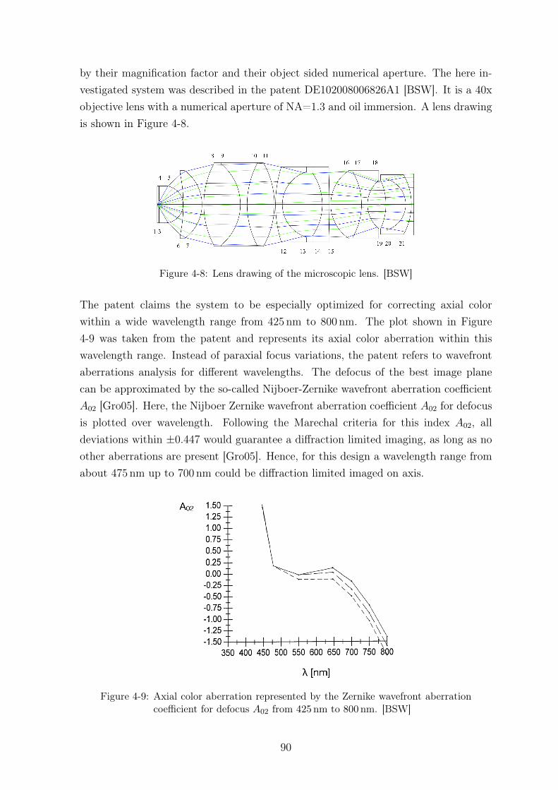
by their magnification factor and their object sided numerical aperture. The here in-vestigated system was described in the patent DE102008006826A1 [BSW]. It is a 40xobjective lens with a numerical aperture of NA=1.3 and oil immersion. A lens drawingis shown in Figure 4-8.

Figure 4-8: Lens drawing of the microscopic lens. [BSW]

The patent claims the system to be especially optimized for correcting axial colorwithin a wide wavelength range from 425 nm to 800 nm. The plot shown in Figure4-9 was taken from the patent and represents its axial color aberration within thiswavelength range. Instead of paraxial focus variations, the patent refers to wavefrontaberrations analysis for different wavelengths. The defocus of the best image planecan be approximated by the so-called Nijboer-Zernike wavefront aberration coefficient𝐴02 [Gro05]. Here, the Nijboer Zernike wavefront aberration coefficient 𝐴02 for defocusis plotted over wavelength. Following the Marechal criteria for this index 𝐴02, alldeviations within ±0.447 would guarantee a diffraction limited imaging, as long as noother aberrations are present [Gro05]. Hence, for this design a wavelength range fromabout 475 nm up to 700 nm could be diffraction limited imaged on axis.

Figure 4-9: Axial color aberration represented by the Zernike wavefront aberrationcoefficient for defocus 𝐴02 from 425 nm to 800 nm. [BSW]

90

Please note, for this plot, a tube lens with a focal length of 164.5 mm, also mentioned inthe patent, was positioned in a distance of 126.5 mm. The tube lens parameters weretaken from [War19] and also include an additional 80 mm NBK7 glass block. Thiscombination of microscope objective lens and tube lens enables the magnification of40x. Although, the patent claims a numerical aperture of NA=1.3, a detailed analysisof the system showed that this microscope lens performs well and almost diffractionlimited for a reasonable object field of 0.5 mm and a numerical aperture of NA=1.0within a wavelength range of 450 nm to 700 nm. A lens drawing of the total designis shown in Figure 4-10 and the summary of the most important performance plots isrepresented by Figure 4-11.

Figure 4-10: Lens drawing of the microscopic lens described in [BSW] combined witha standard tube lens package, described in [War19].

Figure 4-11: Optical Performance plots of the microscopic lens at 𝑁𝐴 = 1.0 (a) Spot diagram,(b) polychromatic MTF, (c) Longitudinal aberration plot and (d) paraxial chro-matic focus shift

91

4.2.2 Design Analysis

The spot diagram in Figure 4-11(a) and the polychromatic MTF plot in Figure 4-11(b)confirm the very high optical performance of the lens. Especially the on axis field pointshows an almost perfectly corrected spot. The root mean square (RMS) spot radiusis 7.85 µm and therefore less than the Airy disc radius of 13.9 µm (for 546 nm), inwhich the diffraction limited resolution is guaranteed. The RMS field point spot sizeis 18.5 µm. Hence, also a very high resolution over the whole field was achieved. Thisbehavior is again verified by the polychromatic MTF plot, where both field points arevery close to the theoretical resolution limit.The most significant plot for the design is the longitudinal aberration diagram. Here,the idea of correction can be seen. Since microscopic lenses are characterized by theirhigh numerical apertures and small object fields, the most critical aberrations areaxial color, spherical aberration and spherochromatism. In most cases, the only wayto correct spherical aberration for such a high aperture system is to find the bestinteraction between 3rd-order and 5th- or even higher order spherical aberration parts.For the patent design, it can be seen that up to a numerical aperture of NA=0.5 aparabolic behavior and therefore a 3rd-order behavior is dominant for all wavelengths.For aperture rays higher than NA=0.5 a first or even a second inflection point ispresent. At these inflection points higher-order aberration become dominant and enablea balancing of the lower order aberration parts. It should be noted, since higher orderaberrations always lead to increased sensitivities of the design, its presence and itsamounts should always be reduced as best as possible by ensuring a high correctionof 3rd-order aberrations up to a high NA, like it was done here. By means of thework of Buchdahl [Buc54], Rimmer [Rim63], Hoffman [Hof93] and Sasian [Sas10] thehere present balancing of 3rd-, 5th- and 7th-order spherical aberration amounts, cancompletely be analyzed surface by surface through the design.Now, within a considerable wavelength range like for the patent case, not only sphericalaberration but also axial color and spherochromatism become performance criticalaberrations. This was especially addressed within the patent. Here, the availableanalyzing tools for an optical designer are more limited and sometimes even less helpfulto understand the system’s way of color correction. For instance, usually first of allthe chromatic focus shift plot, shown in Figure 4-11(d), and a Seidel analysis for axialcolor are investigated. In case of the microscope objective lens, the Seidel diagramsfor axial color of the outer wavelength 450 nm to 700 nm and of secondary color from450 nm to 546 nm are shown in Figures 4-12 and 4-13, respectively.

92

Figure 4-12: Longitudinal Seidel surface coefficients of axial color (1st AXC) for 450 nm and700 nm. Surface numbers 1 to 3 are immersion surfaces. Surface numbers from4 to 21 and 23 to 26 are the microscopic lens surfaces and the tube lens withglass block, respectively. The last bar shows the sum over the total system andits exact values above.

Figure 4-13: Longitudinal Seidel surface coefficients of axial color (1st AXC) for 450 nm and546 nm. Surface numbers are the same as in Figure 4-12.

93

Here, a first misleading result can be found. By comparing the results of the chromaticfocus shift plot to the longitudinal Seidel coefficients, a large deviation of the final axialcolor amounts can be found. Since the focus shift plot is based on a paraxial raytrace,its values are expected to be reproduced by the Seidel analysis. But in case of themicroscopic lens, the Seidel analysis gives a total amount of −1.635 mm instead of−1.945 mm for 450 nm to 700 nm and even only −0.031 mm instead of −0.968 mm for450 nm to 546 nm. Hence, for this design the standard Seidel analysis is not a reliableanalyzing tool.Furthermore, by investigating the paraxial chromatic focus shift plot of Figure 4-11(d)in detail, its result moreover does not meet the exceptions for a diffraction limiteddesign and the corresponding axial color plot of the patent in Figure 4-9. Similar tothe Airy disk diameter for the spot size, the Rayleigh length describes the longitudinalrange within a diffraction limited imaging is possible [Gro05]. Since the Rayleigh lengthfor the microscopic design amounts 0.87 mm, only a very narrow wavelength range of510 nm up to 580 nm would be diffraction limited following the chromatic focus shiftdiagram. Therefore, the interpretation of this plot strongly deviates from the statementof the axial color aberration diagram of the patent, shown in Figure 4-9, which indicatesa diffraction limited imaging from about 475 nm up to 700 nm. In consequence, thisway of analyzing, by only considering the paraxial focus shift, seems to be not enough,since it contradicts the Rayleigh length criteria as well as the statement of the axialcolor plot taken from the patent.

4.2.3 Improved Analysis by the New Theory

Now, to overcome these misleading results of the two standard analyzing tools a lensdesigner can work with, the new surface contribution formulas, found in this thesis,have to be applied. They provide more reasonable results and give an additional deeperunderstanding on how this microscopic lens design works.At first, the 1st-order Seidel coefficient results of Figure 4-12 and 4-13 for the longitu-dinal axial color contributions can be extended by their 2nd-order axial color amounts.For this purpose, the surface contribution formula (3.18) of Section 3.2 converted toits longitudinal description by the conversion factor 1/2𝑛𝑢′2 gives the following, newaxial color surface contribution plots.Comparing these results to the real, raytrace based axial color plot, this extensionof the standard 1st-order Seidel analysis tool with their 2nd-order contributions nowprovides a reliable surface resolved analysis for axial color.

94

Figure 4-14: Longitudinal Seidel surface coefficients of axial color including 1st- and 2nd-ordercontributions for 450 nm and 700 nm. Surface numbers 1 to 3 are immersionsurfaces. Surface numbers from 4 to 21 and 23 to 26 are the microscopic lenssurfaces and the tube lens with glass block, respectively. The last bar shows thesum over the total system and its exact values above.

Figure 4-15: Longitudinal Seidel surface coefficients of axial color including 1st- and 2nd-orderfor 450 nm to 546 nm. Surface numbers are the same as in Figure 4-14.

95

Considering the plots of Figure 4-14 and 4-15 , the new surface coefficient analysis nowgives a total amount of −1.989 mm for 450 nm to 700 nm (instead of −1.945 mm byraytrace) and −0.995 mm for 450 nm to 546 nm (instead of −0.968 mm by raytrace).This reduces the error of the total axial color amount at the image plane for both plotsto less than 3%.Furthermore, a larger influence of the 2nd-order terms on secondary spectrum thanon the outer wavelengths is in evidence. This effect was already described by Wynne[Wyn78], Rogers [Rog13b] and Nobis [Nob15]. It is due to the fact that the 2nd-order color aberration parts introduce an additional bowing to the chromatic focalshift, which is essentially expressed as secondary color and can now be quantitativelyrecovered in Figure 4-15. In case of the microscopic lens, the 2nd-order parts accountmore than 96% of the final axial color value.However, the most significant effect, when adding the 2nd-order terms to the 1st-orderterms, is found in how the single surface contributions, their relation to each otherand their relative input to the overall correction of axial color change. For instance,if only 1st-order Seidel contributions would be considered, surface 16 is the secondlargest negative contributor for secondary color and plays an important role for theoverall correction. But by introducing 2nd-order parts, the contribution of surface 16is almost completely canceled out. In contrast to this, the influence of surface 8 changesfrom one of the weakest negative contributors to the strongest one, since it is almostdoubled by the 2nd-order part. Similar to these two examples, also the surfaces 9 and15 suffer from comparable changes. Please note, besides the impact to the microscopiclens also the tube lens (surfaces 23-24) is affected by 2nd-order terms. Instead ofbeing almost neglectable according to 1st-order, the tube lens does show a relevantcontribution to the overall color correction. This kind of color correction concept ischaracteristic for the here shown microscope system designed by the company ZEISSand would not be visible without 2nd-order.Hence, the new extended analyzing tool reproduces the values of raytrace based chro-matic focus shift plot correctly, shows the right single surface contributions, how theyare balanced by a strong negative front and rear group with a mainly positive actingmiddle group, and gives the correct relative input to the overall color correction at thefinal image plane.

Now, the second misleading result of the standard analyzing tools is addressed. Here,the inconsistency of the paraxial chromatic focus shift plot compared to the Rayleighlength criteria and the proven diffraction limited imaging over the total wavelengthrange has to be solved. Since the axial color plot, taken from the patent 4-9, confirmsthe high performance of the system, the differences between both plots were investi-gated. Following that, the reason for the contradiction can be found in the definition

96

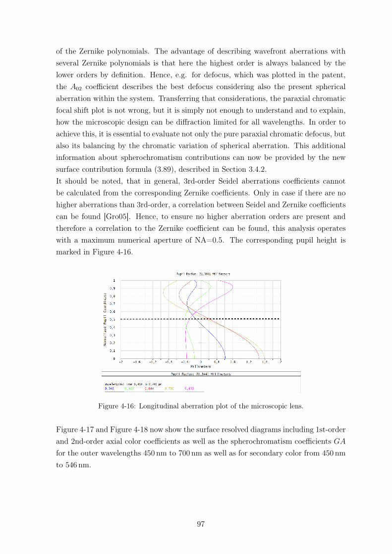
of the Zernike polynomials. The advantage of describing wavefront aberrations withseveral Zernike polynomials is that here the highest order is always balanced by thelower orders by definition. Hence, e.g. for defocus, which was plotted in the patent,the 𝐴02 coefficient describes the best defocus considering also the present sphericalaberration within the system. Transferring that considerations, the paraxial chromaticfocal shift plot is not wrong, but it is simply not enough to understand and to explain,how the microscopic design can be diffraction limited for all wavelengths. In order toachieve this, it is essential to evaluate not only the pure paraxial chromatic defocus, butalso its balancing by the chromatic variation of spherical aberration. This additionalinformation about spherochromatism contributions can now be provided by the newsurface contribution formula (3.89), described in Section 3.4.2.It should be noted, that in general, 3rd-order Seidel aberrations coefficients cannotbe calculated from the corresponding Zernike coefficients. Only in case if there are nohigher aberrations than 3rd-order, a correlation between Seidel and Zernike coefficientscan be found [Gro05]. Hence, to ensure no higher aberration orders are present andtherefore a correlation to the Zernike coefficient can be found, this analysis operateswith a maximum numerical aperture of NA=0.5. The corresponding pupil height ismarked in Figure 4-16.

Figure 4-16: Longitudinal aberration plot of the microscopic lens.

Figure 4-17 and Figure 4-18 now show the surface resolved diagrams including 1st-orderand 2nd-order axial color coefficients as well as the spherochromatism coefficients 𝐺𝐴

for the outer wavelengths 450 nm to 700 nm as well as for secondary color from 450 nm

to 546 nm.

97

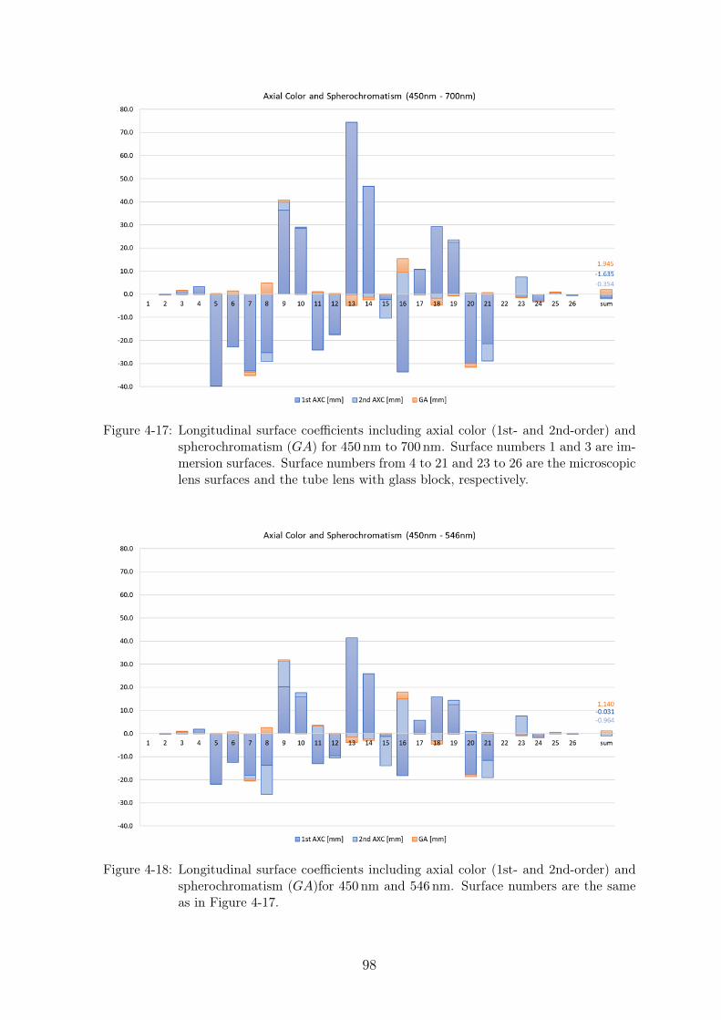
Figure 4-17: Longitudinal surface coefficients including axial color (1st- and 2nd-order) andspherochromatism (𝐺𝐴) for 450 nm to 700 nm. Surface numbers 1 and 3 are im-mersion surfaces. Surface numbers from 4 to 21 and 23 to 26 are the microscopiclens surfaces and the tube lens with glass block, respectively.

Figure 4-18: Longitudinal surface coefficients including axial color (1st- and 2nd-order) andspherochromatism (𝐺𝐴)for 450 nm and 546 nm. Surface numbers are the sameas in Figure 4-17.

98

These two new plots illustrate descriptively the compensation and balancing effects ofaxial color and spherochromatism through the whole optical system and at the finalimage plane. Although the single surface contributions of spherochromatism are muchsmaller than the axial color ones, they finally reach a relevant amount at the imageplane. This is caused by their signs, since for almost all surfaces the spherochromatismparts show the opposite sign than the axial color ones. In both cases, adding upthe spherochromatism contributions leads to an total sum of 1.945 mm for 450 nm to700 nm and 1.140 mm for secondary color, which balances the corresponding large axialcolor values of −1.989 mm and −0.995 mm to a final color contribution smaller thanthe Rayleigh length.Although this new way of analyzing the on axis chromatic errors can only be appliedwithin an numerical aperture, where no higher aberrations than 3rd-order are present,this analyzing tool finally explains how the microscopic lens works. Only the combina-tion of axial color and spherochromatism enables the diffraction limited imaging. Thenew plots demonstrate descriptively how they are balanced and where the dominatingsurfaces and lenses are. Comparing this to the misleading standard Seidel surface coef-ficient plot, these extended analysis now enables the optical designer to understand themicroscopic system and to find the best surfaces or lenses to even improve the design.For example, as stated before, since higher order aberrations always lead to increasedsensitivities of the system, its present and its amounts should always be reduced as bestas possible by ensuring a high correction of 3rd-order aberrations up to a high NA. Thisdesign goal now can directly be addressed by optimizing the system to compensate thehere plotted axial color and spherochromatism for a even larger numerical apertures,e.g. NA=0.6.Finally, to complete the detailed analysis of the microscopic lens, the new found surfacedescription not only allows to analyze the relation between 1st- order and 2nd-orderaxial color as well as spherochromatism, it also enables the designer to distinguishbetween intrinsic and induced aberration parts. The corresponding diagrams for sec-ondary color are shown in Figure 4-19 and 4-20 for axial color and spherochromatism,respectively.

99

Figure 4-19: Longitudinal surface coefficients of axial color, distinguishing between intrinsicand induced aberration parts. Surface numbers 1 and 3 are immersion surfaces.Surface numbers from 4 to 21 and 23 to 26 are the microscopic lens surfaces andthe tube lens with glass block, respectively.

Figure 4-20: Longitudinal surface coefficients of spherochromatism, distinguishing betweenintrinsic and induced aberration parts. Surface numbers are the same as inFigure 4-19.

100

The here shown diagrams demonstrate clearly the high influence of induced aberrationson the performance of the microscope lens. Especially for axial color, some inducedparts reach out almost the same amounts as the intrinsic ones or as for surface 15 and23 also exceed them. The most impact of induced axial color aberrations can be foundwithin the middle part of the microscopic objective from surface 8 to 16. Since thefirst three lenses of the objective essentially correct spherical aberration, implying highrefractive glasses and meniscus shaped lenses, a large amount of 1st-order axial colorsum up within this front group. This introduced 1st-order axial color generates theprominent induced color aberration amounts within the middle group. However, theinduced parts of the tube lens is not directly a consequence of a very large 1st-orderaxial color summed before in the microscopic objective, but it is mainly caused bythe huge distance between the microscope and tube lens. Hence, although the priorsummed axial in front of the tube lens is relatively small, the separation of wavelengthat the first surface of the tube becomes comparable large to the separation at surface 8,which is the first surface of the middle group. Figure 4-21 shows, how the wavelengthsare separated at surface 8 and the tube lens.

Figure 4-21: Separation of the different wavelengths at the first surface of the middle groupof the microscopic lens as well as at the first surface of the tube lens.

Regarding spherochromatism, the influences of the induced aberrations are comparablesmall to the axial color ones. Mainly, surface 8 and surface 13 show a relevant amount.The reason for surface 8 can again be found in the large prior summed up 1st-order axialcolor. However, surface 13 shows no noticeable amount for induced axial color, but forspherochromatism this is the strongest contributor for induced and intrinsic parts. Theexplanation is found in the large incident angles 𝑖 at this surface, which can also beseen in Figure 4-8. Here, surface 13 is the cemented surface of the second triplet, whichis extremely bent. Since the induced as well as the intrinsic terms are linear dependingon 𝑖, this extremely bent cemented surface is the key surface for spherochromatism andhas to be observed very carefully during an optimization process.Finally, at the image plane, for both aberrations, axial color and spherochromatism,the intrinsic and the induced parts are well balanced. Therefore, the overall diffractionlimited performance can again be seen here.

101

5 Summary

The major focus of this work was devoted to the investigation of higher-order coloraberrations and their induced and intrinsic aberration parts. In analogous manner tothe monochromatic aberrations, lower-order aberrations, picked up surface by surface inthe preceding optical system, generate induced aberrations of higher order. However,contrary to monochromatic aberrations, induced influences of color aberrations arealready observable in the paraxial regime, since even paraxial rays are affected bydispersion.Consequently, at first a new classification of aberration orders was introduced in thesis,since, in case of color aberrations, different orders do not refer to the ray dependencyon field and pupil coordinates only. This work extended the aberration theory tohigher-order effects regarding the ray dependency on dispersion.Following that, a new analytical approach was described, investigating the influence ofdispersion, starting at the paraxial parameters of the intersection length and the imageheight up to its impact on 3rd-order monochromatic aberrations. Based on the cumu-lative characteristics of induced aberrations, a surface and lens resolved descriptionswas required. In Section 3.2, 3.3, 3.4 and 3.5 a complex analytical analysis showed,that the influence of dispersion can always be identified by the small chromatic differ-ences in ray heights (∆𝑦 and ∆𝑦) and ray angles (∆𝑢 and ∆�̄�) of the marginal andchief ray within the optical system. In overcoming the analytical gap for induced coloraberrations discussed in Section 2.5, the essential analytical finding of this thesis werefour equations, (3.107), (3.108), (3.109) and (3.110), representing the direct relation ofthe marginal and chief ray variations to prior summed up 1st-order color aberrations,𝐴𝑋𝐶 and 𝐿𝐴𝐶, and pupil color aberrations, 𝐴𝑋𝐶𝑝 and 𝐿𝐴𝐶𝑝. Considering these re-lations, the calculation of 2nd-order axial and lateral color as well as of the chromaticvariations of spherical aberration, coma, astigmatism, field curvature and distortion,distinguishing between intrinsic and induced aberration parts, were enabled.These new surface coefficient formulas provides the optical designer a new analysistool to get a deeper understanding of how and why induced color aberration occur.Hence, in the second part of this work, at first five classical and academic examples forinduced color aberrations were discussed. All of them are kept very simple in design,since those are best for understanding the characteristics and possible influences of 2nd-

102

order induced and intrinsic color aberrations. Particularly, the catadioptric system in4.1.4 and the split achromat in 4.1.5 are often-cited examples for induced color effects.However, an exact analytical analysis and therefore also a deeper understanding ofthem was missing. Here, the new surface contribution formulas, found in this thesis,were applied and explained how these designs work.Finally, since a more complex design example represents a higher relevance for thepractical work of an optical designer, the final system example was a complex micro-scope objective lens. Here, a system of many lenses within a compact arrangement anda multitude of different glass combinations was presented. A detailed design analysisshowed, that by considering the available standard analysis tools for color aberrations,like Seidel’s surface coefficients and a chromatic focus shift plot, misleading resultsoccurred. Only, by extending those standard tools with the new 2nd-order axial colorsurface coefficients and by adding up the balancing parts of spherochromatism, thepresent diffraction limited imaging can be explained. The new surface coefficient plotsdemonstrated descriptively how the intrinsic and induced 1st-order and 2nd-order ax-ial color as well as spherochromatism parts were balanced and where the dominatingsurfaces and lenses were. Comparing this to the misleading standard Seidel surfacecoefficient plot, these extended analysis enabled the optical designer to understand themicroscopic system and to find the best surfaces or lenses to even improve the design.

103

A Appendix

A.1 Induced Axial Color

1st-order derivatives for axial color:

𝜕𝑠

𝜕𝑦= −1

𝑢

𝜕𝑠

𝜕𝑢=

𝑦

𝑢2

𝜕𝑠′

𝜕𝑦= − 𝑛𝑢

𝑛′𝑢′2

𝜕𝑠′

𝜕𝑢=

𝑛𝑦

𝑛′𝑢′2

𝜕𝑠′

𝜕𝑛=

𝑦𝑖

𝑛′𝑢′2

𝜕𝑠′

𝜕𝑛′ = − 𝑛𝑦𝑖

𝑛′2𝑢′2

2nd-order derivatives for axial color:

𝜕2𝑠

𝜕𝑦2= 0

𝜕2𝑠

𝜕𝑢2= −2𝑦

𝑢3

𝜕2𝑠′

𝜕𝑦2= −𝑛𝑢𝑐(𝑛′ − 𝑛)

𝑛′2𝑢′3

𝜕2𝑠′

𝜕𝑢2= − 𝑛2𝑦

𝑛′2𝑢′3𝑢

𝜕2𝑠′

𝜕𝑛2= − 𝑦𝑖2

𝑛′2𝑢′3

𝜕2𝑠′

𝜕𝑛′2 = −𝑦2𝑛𝑖𝑐

𝑛′3𝑢′3

i

𝜕2𝑠

𝜕𝑦𝜕𝑢=

1

𝑢2

𝜕2𝑠′

𝜕𝑦𝜕𝑢=

𝑛(𝑛′ − 𝑛)𝑦𝑐 + 𝑛2𝑢

𝑛′2𝑢′3

𝜕2𝑠′

𝜕𝑦𝜕𝑛=

𝑢(𝑛′ − 𝑛)𝑦𝑐 + 𝑛𝑢2 + 2𝑛𝑢𝑦𝑐

𝑛′2𝑢′3

𝜕2𝑠′

𝜕𝑦𝜕𝑛′ = −−𝑛2𝑢2 + 𝑛𝑢(𝑛′ − 𝑛)𝑦𝑐− 2𝑛′𝑛𝑢𝑦𝑐

𝑛′3𝑢′3

𝜕2𝑠′

𝜕𝑢𝜕𝑛=

−𝑦2(𝑛′ − 𝑛)𝑐− 𝑛𝑦𝑢− 2𝑛𝑦2𝑐

𝑛′2𝑢′3𝑢

𝜕2𝑠′

𝜕𝑢𝜕𝑛′ =𝑛𝑢′𝑦 + 2𝑛𝑦2𝑐

𝑛′2𝑢′3

𝜕2𝑠′

𝜕𝑛𝜕𝑛′ =𝑛𝑦𝑖2 + 𝑛′𝑦2𝑖𝑐

𝑛′3𝑢′3

Equation (3.23). Coefficients 𝛼1 and 𝛼2 of the thick lens formula for axial color:

𝛼1 = 2𝑢1𝑐2 + 2𝑦1𝑐1𝐹2

𝛼2 = 𝑛𝑢31 − 𝑐2𝑢

21𝑦1 − 𝑐21𝑦

31𝐹2 + 3𝑐22𝑛𝑢1𝑦

21 − 2𝑐1𝑐2𝑢1𝑦

21 + 3𝑐2𝑛𝑢

21𝑦1

+ 3𝑐22𝑡𝑛𝑢21𝑦1 + 2𝑐2𝑡𝑛𝑢

31 + 𝑐22𝑡

2𝑛𝑢31

A.2 Induced Lateral Color

1st-order derivatives for lateral color:

𝜕𝑦1𝜕𝑦

= 1

𝜕𝑦1𝜕�̄�

= 𝑠

𝜕𝑦′1𝜕𝑦

= 1 − 𝑠′(𝑛′ − 𝑛)𝑐

𝑛′

𝜕𝑦′1𝜕�̄�

= −𝑠′𝑛

𝑛′

𝜕𝑦′1𝜕𝑛

=𝑠′̄𝑖

𝑛′

𝜕𝑦′1𝜕𝑛′ = −𝑛𝑠′̄𝑖

𝑛′2

ii

2nd-order derivatives for lateral color:

𝜕2𝑦1𝜕𝑦2

=𝜕2𝑦1𝜕𝑦𝜕�̄�

=𝜕2𝑦1𝜕�̄�2

=𝜕2𝑦′1𝜕𝑦2

=𝜕2𝑦′1𝜕𝑦𝜕�̄�

=𝜕2𝑦′1𝜕�̄�2

=𝜕2𝑦′1𝜕𝑛2

= 0

𝜕2𝑦′1𝜕𝑦𝜕𝑛

=𝑠′𝑐

𝑛′

𝜕2𝑦′1𝜕𝑦𝜕𝑛′ = −𝑠′𝑛𝑐

𝑛′2

𝜕2𝑦′1𝜕�̄�𝜕𝑛

=𝑠′

𝑛′

𝜕2𝑦′1𝜕�̄�𝜕𝑛′ = −𝑠′𝑛

𝑛′2

𝜕2𝑦′1𝜕𝑛𝜕𝑛′ = − 𝑠′̄𝑖

𝑛′2

𝜕2𝑦′1𝜕𝑛′2 =

2𝑠′𝑛�̄�

𝑛′3

Equation (3.64). Coefficients 𝛽1 and 𝛽2 of the thick lens formula for lateral color

𝛽1 = 2𝑦1𝑢1𝑐2 + 𝑢21 + 𝑡𝑢2

1𝑐2

𝛽2 = − 𝑦1�̄�1𝑐2 − 𝑢1�̄�1 − 𝑦1𝑢1𝑐2 − 𝑡𝑢1�̄�1𝑐2

A.3 Induced Spherochromatism

1st-order derivatives for spherochromatism:

𝜕𝑆1

𝜕𝑦= −𝑖𝑛(𝑛− 𝑛′)((𝑢− 2𝑖)2 + (4𝑖− 3𝑢)𝑢′)

𝑛′

𝜕𝑆1

𝜕𝑢= (𝑢− 𝑢′)(4𝑖′𝑛′ − 𝑛𝑢 + 3𝑛𝑢′)𝑦

𝜕𝑆1

𝜕𝑛= 𝑖(𝑖′𝑢− 𝑖′2 + 𝑢2 − (2𝑖′ + 𝑢)𝑢′)𝑦

𝜕𝑆1

𝜕𝑛′ = 𝑖′2(𝑖′ + 𝑢′)𝑦

iii

Equation (3.93). Coefficients 𝛾1,𝛾2 and 𝛾3 of the thin lens formula for spherochroma-tism:

𝛾1 = 𝑖20 + 𝑖′1𝑛𝐿(𝑖′1 + 𝑢0) + 𝑖0(𝑖′1 + 𝑛𝐿𝑢0)

𝛾2 = 𝑖′1 + 3𝑖′1𝑛𝐿 + 𝑖0(3 + 𝑛𝐿) + 2𝑛𝐿𝑢0

𝛾3 = 𝑖20(𝑛𝐿 − 2) + 𝑖0𝑛𝐿(2𝑖′1𝑛𝐿 − 3𝑖′1 − 𝑢0) + 𝑖′1𝑛𝐿(2𝑖′1 − 3𝑖′1𝑛𝐿 + 𝑢0 − 2𝑛𝐿𝑢0)

iv

Bibliography

[Ber+15] A. Berner et al. “Chromatic Variation of Aberration: The Role of InducedAberrations and Raytrace Direction”. In: vol. 9626. 2015.

[Ber+18] A. Berner et al. “3rd-Order Spherochromatism Surface Contribution andIts Intrinsic and Induced Aberration Parts”. In: J. Opt. Soc. Am. A 35.8(Aug. 2018), pp. 1368–1378.

[BNG17] A. Berner, T. Nobis, and H. Gross. “Induced Axial and Lateral Color Sur-face Contributions”. In: J. Opt. Soc. Am. A 34.5 (May 2017), pp. 685–695.

[BSW] M. Brehm, R. Shi, and R. Wartmann. “Mikroskopobjektiv”. DE102008006826A1.

[Buc54] H.A. Buchdahl. Optical Aberration Coefficients. Oxford University Press,1954.

[CK92] A.E. Conrady and R. Kingslake. Applied Optics and Optical Design. Ap-plied Optics and Optical Design Bd. 1. Dover Publications, 1992. isbn:978-0-486-67007-2.

[Con14] A.E. Conrady. Applied Optics and Optical Design, Part Two. Dover Bookson Physics. Dover Publications, 2014. isbn: 978-0-486-16262-1.

[Del52] E. Delano. “A General Contribution Formula for Tangential Rays”. In: J.Opt. Soc. Am. 42.9 (Sept. 1952), pp. 631–633.

[Gro+07] H. Gross et al. Handbook of Optical Systems, Aberration Theory and Correc-tion of Optical Systems. Handbook of Optical Systems. Wiley, 2007. isbn:978-3-527-40379-0.

[Gro05] H. Gross. Handbook of Optical Systems, Fundamentals of Technical Optics.Handbook of Optical Systems. Wiley, 2005. isbn: 978-3-527-40377-6.

[Haf86] H. Haferkorn. Bewertung Optischer Systeme. Optisches Instrument. VEBDeutscher Verlag der Wissenschaften, 1986. isbn: 978-3-326-00000-8.

[Hof] C. Hofmann. “Die Bewertung Optischer Systeme”. In: Fortschritte der Physik27.11-12 (), pp. 595–639.

[Hof93] J. M. Hoffman. Induced Aberrations in Optical Systems. The University ofArizona., 1993.

v

[Hop50] H.H. Hopkins. Wave Theory of Aberrations. Monographs on the Physicsand Chemistry of Materials. Clarendon Press, 1950.

[Ker95] A. Kerber. Beiträge Zur Dioptrik. Vol. Erstes Heft. Selbstverlag, Leipzig,1895.

[Kin12] R. Kingslake. Lens Design Fundamentals. Elsevier Science, 2012. isbn: 978-0-08-051009-5.

[KT02] M.J. Kidger and V.V. Tuchin. Fundamental Optical Design. Press Mono-graphs. Society of Photo Optical, 2002. isbn: 978-0-8194-3915-4.

[Mcc55] E. L. Mccarthy. “Optical System with Corrected Secondary Spectrum”. In:(Jan. 1955). US Patent 2,698,555.

[MM17] D. Malacara-Hernández and Z. Malacara-Hernández. Handbook of OpticalDesign. CRC Press, 2017. isbn: 978-1-351-83292-2.

[Nak15] H. Nakajima. Optical Design Using Excel: Practical Calculations for LaserOptical Systems. Wiley, 2015. isbn: 978-1-118-93914-7.

[Nob14] T. Nobis. “A Lens-Resolved Approach for Analyzing and Correcting Sec-ondary Axial Color”. In: Classical Optics 2014. Classical Optics 2014. Op-tical Society of America, 2014, ITu1A.1.

[Nob15] T. Nobis. “Second-Order Axial Color of Thin Lenses in Air”. In: J. Opt.Soc. Am. A 32.10 (Oct. 2015), pp. 1857–1869.

[Rim63] M.P. Rimmer. Optical Aberration Coefficients. 1963.

[Rog13a] J. R. Rogers. “Secondary Color Correction and Tolerance Sensitivity: WhatCan You Get Away With?” In: vol. 8844. 2013.

[Rog13b] J. R. Rogers. “The Importance of Induced Aberrations in the Correctionof Secondary Color”. In: Advanced Optical Technologies 2.1 (2013), p. 41.issn: 21928584.

[Sas10] J. Sasián. “Theory of Sixth-Order Wave Aberrations”. In: Appl. Opt. 49.16(June 2010), pp. D69–D95.

[Sei56] L. Seidel. “Zur Dioptrik. Ueber Die Entwicklung Der Glieder 3ter Ordnung,Welche Den Weg Eines Ausserhalb Der Ebene Der Axe Gelegenen Licht-strahles Durch Ein System Brechender Medien Bestimmen, von Herrn Dr.L. Seidel”. In: Astronomische Nachrichten 43.19 (1856), pp. 289–304.

[Sli84] G. G. Sliusarev. “Aberration and Optical Design Theory”. In: Bristol, Eng-land, Adam Hilger, Ltd., 1984, 672 p. Translation. (1984).

[Smi04] W. Smith. Modern Lens Design. Electronic Engineering. Mcgraw-hill, 2004.isbn: 978-0-07-143830-8.

vi

[Smi66] W. J. Smith. Modern Optical Engineering. McGraw-Hill, 1966.

[War19] R. Wartmann. “Apochromatisches Mikroskopobjektiv Und Mikroskop”. DE102017218169B3. Mar. 2019.

[Wel86] W. T. Welford. Aberrations of Optical Systems. Series in Optics and Opto-electronics. Taylor & Francis, 1986. isbn: 978-0-85274-564-9.

[Wyn77] C. G. Wynne. “Secondary Spectrum Correction with Normal Glasses”. In:Optics Communications 21.3 (June 1977), pp. 419–424. issn: 0030-4018.

[Wyn78] C. G. Wynne. “A Comprehensive First-Order Theory of Chromatic Aberra-tion. Secondary Spectrum Correction without Special Glasses”. In: OpticaActa: International Journal of Optics 25.8 (1978), pp. 627–636.

[Zim67] H.-G. Zimmer. Geometrische Optik. Springer Verlag, Berlin, Heidelberg,NewYork, 1967.

vii

List of Figures

2-1 Paraxial approximation of imaging, assuming all rays starting at onepoint of the object plane 𝑂𝑃 perfectly meeting at an image point of theconjugated image plane 𝐼𝑃 . . . . . . . . . . . . . . . . . . . . . . . . . 8

2-2 Refraction at an optical surface, assuming rotational symmetry alongz-axis. . . . . . . . . . . . . . . . . . . . . . . . . . . . . . . . . . . . . 10

2-3 Paraxial ray transfer at an arbitrary surface 𝑗 of an optical system tosurface 𝑗 + 1. . . . . . . . . . . . . . . . . . . . . . . . . . . . . . . . . 12

2-4 Refraction of the marginal ray (solid line) and the chief ray (dashed line)at a thick lens. . . . . . . . . . . . . . . . . . . . . . . . . . . . . . . . 14

2-5 Real imaging of an optical system, considering real optics with finite rayheights and ray angles. . . . . . . . . . . . . . . . . . . . . . . . . . . . 15

2-6 Definition of wavefronts as a surface of constant optical path lengthmeasured from a point at the object plane. . . . . . . . . . . . . . . . . 16

2-7 Wavefront aberration defined as the deviation of the wavefront to areference sphere (dotted line). This is determined by the paraxial imagepoint O’ as center and the intersection point of the chief ray with theoptical axis. . . . . . . . . . . . . . . . . . . . . . . . . . . . . . . . . . 17

2-8 Definition of field vector 𝐹 at the object plane and pupil vector 𝑃 atthe pupil plane of an optical system. . . . . . . . . . . . . . . . . . . . 18

2-9 Transverse ray aberration ∆𝑦′ in the y-z-plane of an optical system. . . 202-10 Lens example with three surfaces, forming a real intermediate image in

each space in between the surfaces. . . . . . . . . . . . . . . . . . . . . 222-11 Variation of the refractive index n with wavelength for BK7 . . . . . . 242-12 Abbe diagram of the manufacturer Schott . . . . . . . . . . . . . . . . 262-13 Partial Dispersion of the manufacturer Schott . . . . . . . . . . . . . . 262-14 Axial color aberration ∆𝑠′ of a single positive thin lens . . . . . . . . . 272-15 Achromatic case, where the blue and red foci show the same intersection

length. The green focal length is shorter. . . . . . . . . . . . . . . . . 282-16 Lateral color ∆𝑦′ of a single positive thin lens . . . . . . . . . . . . . . 292-17 Bar plots of Seidel surface contribution for a given lens design. . . . . 31

viii

2-18 Monochromatic intrinsic and induced ray aberration parts . . . . . . . 33

3-1 Intrinsic and induced color aberration parts . . . . . . . . . . . . . . . 373-2 Classification of different color aberration orders exemplary shown, start-

ing at (a) paraxial intersection lengths s and (b) image height y. Thegreen and yellow colored quantities mark the well-known Seidel andBuchdahl coefficients, respectively. The blue framed quantities includeinduced color aberrations. . . . . . . . . . . . . . . . . . . . . . . . . . 38

3-3 Overview of the current state of the induced color aberration problemand the new derived quantities within this thesis. Please note, SinceWynne identified a way to determine the contribution of induced axialand lateral color by tracing two paraxial rays with different wavelengths,his induced terms are not wrong, but can be simplified within this newapproach. . . . . . . . . . . . . . . . . . . . . . . . . . . . . . . . . . . 39

3-4 Refraction of two paraxial marginal rays with different wavelengths (blackand blue line) at an arbitrary surface S . . . . . . . . . . . . . . . . . . 40

3-5 Refraction of the marginal ray at a thick lens. The marginal ray heightsand angles are 𝑦1 and 𝑢1 as well as 𝑦2 and 𝑢2 at surface S1 and surfaceS2, respectively. . . . . . . . . . . . . . . . . . . . . . . . . . . . . . . . 44

3-6 Refraction of two paraxial chief rays with different wavelengths (blackand blue line) at an arbitrary surface S. The intermediate images showdifferent lateral color aberrations ∆𝑦1 and ∆𝑦′1 , whereby the imageposition is defined by the intersection length of the marginal ray (dashedline) . . . . . . . . . . . . . . . . . . . . . . . . . . . . . . . . . . . . . 47

3-7 Refraction of two paraxial chief rays with different wavelengths (blackand blue line) at an arbitrary surface S. The intermediate images showlateral color aberrations ∆𝑦1 and ∆𝑦′1, which also leads to a chromaticdefocused image of the stop position ∆𝑝. . . . . . . . . . . . . . . . . . 52

3-8 Refraction of the marginal ray and chief ray (dashed and solid line) ata thick lens with an refractive index of n. The marginal ray heights andangles are 𝑦1 and 𝑢1 as well as 𝑦2 and 𝑢2 at surface S1 and surface S2,respectively. The chief ray heights and angles are 𝑦0 and �̄�0, 𝑦1 and �̄�1

as well as 𝑦2 and �̄�2 at the intermediate image, surface S1 and surfaceS2, respectively. . . . . . . . . . . . . . . . . . . . . . . . . . . . . . . . 54

3-9 Parameters defining the spherical aberration conditions. Here, capitalletters refer to real ray and small letter to the paraxial ray parameters. 58

ix

3-10 Quantities defining spherochromatism. Here, the solid black line param-eters refer to the real ray path and dashed black line parameters to theparaxial ray path of the primary wavelength 𝜆1. The second wavelength𝜆2 is represented by blue lines. Again, capital letters belong to the realrays and small letters to the paraxial rays. . . . . . . . . . . . . . . . . 59

3-11 Longitudinal aberration plot corresponding to the relations, shown inFigure 3-10 for wavelength 𝜆1 and wavelength 𝜆1. Here, the intersectionlength s for 𝜆1 provides the reference. ∆𝑠 describes the difference inz-direction to this reference and ℎ𝑝 characterizes the relative pupil height. 60

3-12 Extended considerations on a chromatically varying marginal ray. Here,the solid line parameters again refer to the marginal ray of the primarywavelength 𝜆1 and the blue line parameters to the marginal ray of thesecond wavelength 𝜆2. Additionally, the chief ray of 𝜆1 is plotted as adotted line. The intersection length s of the marginal ray characterizesthe intermediate image for 𝜆1. At this image, an axial color aberration∆𝑠 is present. The position of the imaged stop in front of the surface isdefined by the intersection length p of the chief ray. Here, a chromaticvarying stop size characterized by ∆𝑦𝑝 is present. The same considera-tions are applied for the primed quantities after the surface. . . . . . . 63

4-1 Example design composed of two lenses, each in a 4f- arrangement. (a)shows the marginal raytrace for two different wavelengths (dashed anddotted line), illustrating the axial color parameters and (b) shows thechief raytrace of two different wavelengths (solid and dotted line) illus-trating the lateral color parameters. . . . . . . . . . . . . . . . . . . . . 74

4-2 Thick meniscus lens with same radii of 𝑅 = 15 mm and a thickness of𝑡 = 10 mm. . . . . . . . . . . . . . . . . . . . . . . . . . . . . . . . . . . 77

4-3 (a) Schupmann achromatic design, where a positive lens with 𝑓 ′𝐿1 and

negative lens with 𝑓 ′𝐿2 = −𝑓 ′

𝐿1 are set up together, separated by anairspace of 𝑑 = 2𝑓 ′

𝐿1. (b) Schupmann design improved by a third lenswith 𝑓 ′

𝐿3 = 1/2𝑓 ′𝐿1, positioned exactly at the intermediate image between

the two lenses. . . . . . . . . . . . . . . . . . . . . . . . . . . . . . . . . 784-4 Longitudinal aberration plots for (a) the two-lenses N-BK7 Schupmann

design and (b) the same Schupmann design improved by a third N-BK7thin lens with positioned exactly at the intermediate image between thetwo lenses. . . . . . . . . . . . . . . . . . . . . . . . . . . . . . . . . . . 79

4-5 Thick meniscus lens with same radii of 𝑅 = 15 mm and a thickness of𝑡 = 10 mm. . . . . . . . . . . . . . . . . . . . . . . . . . . . . . . . . . . 82

x

4-6 (a) a classical unsplit achromat and (b) a split achromat with a air spacebetween the lenses. . . . . . . . . . . . . . . . . . . . . . . . . . . . . . 85

4-7 Longitudinal aberration plots for (a) the classical unsplit achromat and(b) the split achromat with a air space between the lenses. The first,positive lens is made of NBK7 and the second, negative lens of NSF5. . 85

4-8 Lens drawing of the microscopic lens. [BSW] . . . . . . . . . . . . . . 904-9 Axial color aberration represented by the Zernike wavefront aberration

coefficient for defocus 𝐴02 from 425 nm to 800 nm. [BSW] . . . . . . . 904-10 Lens drawing of the microscopic lens described in [BSW] combined with

a standard tube lens package, described in [War19]. . . . . . . . . . . . 914-11 Optical Performance plots of the microscopic lens at 𝑁𝐴 = 1.0 (a) Spot

diagram, (b) polychromatic MTF, (c) Longitudinal aberration plot and(d) paraxial chromatic focus shift . . . . . . . . . . . . . . . . . . . . . 91

4-12 Longitudinal Seidel surface coefficients of axial color (1st AXC) for450 nm and 700 nm. Surface numbers 1 to 3 are immersion surfaces.Surface numbers from 4 to 21 and 23 to 26 are the microscopic lenssurfaces and the tube lens with glass block, respectively. The last barshows the sum over the total system and its exact values above. . . . . 93

4-13 Longitudinal Seidel surface coefficients of axial color (1st AXC) for450 nm and 546 nm. Surface numbers are the same as in Figure 4-12. . 93

4-14 Longitudinal Seidel surface coefficients of axial color including 1st- and2nd-order contributions for 450 nm and 700 nm. Surface numbers 1 to3 are immersion surfaces. Surface numbers from 4 to 21 and 23 to 26are the microscopic lens surfaces and the tube lens with glass block,respectively. The last bar shows the sum over the total system and itsexact values above. . . . . . . . . . . . . . . . . . . . . . . . . . . . . . 95

4-15 Longitudinal Seidel surface coefficients of axial color including 1st- and2nd-order for 450 nm to 546 nm. Surface numbers are the same as inFigure 4-14. . . . . . . . . . . . . . . . . . . . . . . . . . . . . . . . . . 95

4-16 Longitudinal aberration plot of the microscopic lens. . . . . . . . . . . 974-17 Longitudinal surface coefficients including axial color (1st- and 2nd-

order) and spherochromatism (𝐺𝐴) for 450 nm to 700 nm. Surface num-bers 1 and 3 are immersion surfaces. Surface numbers from 4 to 21 and23 to 26 are the microscopic lens surfaces and the tube lens with glassblock, respectively. . . . . . . . . . . . . . . . . . . . . . . . . . . . . . 98

4-18 Longitudinal surface coefficients including axial color (1st- and 2nd-order) and spherochromatism (𝐺𝐴)for 450 nm and 546 nm. Surface num-bers are the same as in Figure 4-17. . . . . . . . . . . . . . . . . . . . . 98

xi

4-19 Longitudinal surface coefficients of axial color, distinguishing betweenintrinsic and induced aberration parts. Surface numbers 1 and 3 areimmersion surfaces. Surface numbers from 4 to 21 and 23 to 26 are themicroscopic lens surfaces and the tube lens with glass block, respectively. 100

4-20 Longitudinal surface coefficients of spherochromatism, distinguishing be-tween intrinsic and induced aberration parts. Surface numbers are thesame as in Figure 4-19. . . . . . . . . . . . . . . . . . . . . . . . . . . . 100

4-21 Separation of the different wavelengths at the first surface of the middlegroup of the microscopic lens as well as at the first surface of the tubelens. . . . . . . . . . . . . . . . . . . . . . . . . . . . . . . . . . . . . . 101

xii

List of Tables

4.1 Axial color contributions for the example system for case (1). The wave-length range is 𝜆1 = 486 nm to 𝜆2 = 656 nm. . . . . . . . . . . . . . . . 74

4.2 Axial color contributions for the example system for case (2). The wave-length range is 𝜆1 = 486 nm to 𝜆2 = 656 nm. . . . . . . . . . . . . . . . 75

4.3 Lateral color contributions for the example system for case (1). Thewavelength range is 𝜆1 = 486 nm to 𝜆2 = 656 nm. . . . . . . . . . . . . 75

4.4 Lateral color contributions for the example system for case (2). Thewavelength range is 𝜆1 = 486 nm to 𝜆2 = 656 nm. . . . . . . . . . . . . 76

4.5 Induced and intrinsic axial color contributions of a meniscus lens for awavelength range from 486 nm (F-line) to 587 nm (d-line). . . . . . . . 78

4.6 𝐺𝐿 coefficients of the two-lens Schupmann design for the prior summedup 1st-order color aberrations 𝐴𝑋𝐶𝐿 and 𝐿𝐴𝐶𝐿

𝑝 and the intrinsic andinduced parts of 𝐺𝐿 . . . . . . . . . . . . . . . . . . . . . . . . . . . . . 80

4.7 Seidel wavefront aberration coefficient 𝑆𝐼 by two single ray traces andthe comparison to the spherochromatic coefficient 𝐺. . . . . . . . . . . 82

4.8 Wavefront aberration coefficients of the mirror design example for theprior summed up chromatic aberrations 𝐴𝑋𝐶1𝑠𝑡 and 𝐿𝐴𝐶𝑝,1𝑠𝑡 and theintrinsic and induced parts of 𝐺. . . . . . . . . . . . . . . . . . . . . . . 83

4.9 Conversation of Seidel’s spherical aberration coefficients and of the sphe-rochromatism coefficient 𝐺 into longitudinal aberrations 𝑆𝑃𝐻 and 𝐺𝐴 84

4.10 Numerical solution for three variable radii 𝑅1, 𝑅2 and 𝑅3 of the unsplitachromat. The Seidel contributions for axial color 𝐴𝑋𝐶 and 3rd-orderspherical aberration 𝑆𝐼 as well as the Buchdahl-Rimmer 5th-order con-tributions 𝐵5 are given. . . . . . . . . . . . . . . . . . . . . . . . . . . 86

4.11 Numerical solution for three variable radii 𝑅2, 𝑅3, 𝑅4 and a variableair space thickness t of the split achromat. The Seidel contribution foraxial color 𝐴𝑋𝐶 and 3rd-order spherical aberration 𝑆𝐼 as well as theBuchdahl-Rimmer 5th-order contributions 𝐵5 and the Spherochroma-tism contributions 𝐺 are given. . . . . . . . . . . . . . . . . . . . . . . 88

xiii

4.12 Numerical solution for three variable radii 𝑅2, 𝑅3, 𝑅4 and a variable airspace thickness t of the split achromat. The spherochromatism contri-butions 𝐺 and its intrinsic as well as its induced parts are given. . . . . 89

xiv

Zusammenfassung

Der Schwerpunkt dieser Arbeit lag auf der Untersuchung von Farbaberrationen höhererOrdnung sowie der Differenzierung ihrer induzierten und intrinsischen Aberrationsan-teile.In analoger Weise zu den monochromatischen Abbildungsfehlern, erzeugen Fehler niedrig-erer Ordnung induzierte Fehler höherer Ordnung, welche sich Fläche für Fläche inner-halb des optischen System aufsummieren. Diese induzierten Aberrationsanteile ex-istieren im Falle der Farbfehler jedoch bereits im paraxialen Bereich, da auch paraxialeStrahlen durch Dispersion beeinflusst werden.Folglich wurde in dieser Arbeit zunächst eine neue Klassifikation der Aberrationsord-nungen eingeführt. Im Falle von Farbfehlern beziehen sich die unterschiedliche Ord-nungen neben der Feld- und Pupillenabhängigkeiten der Strahlen zusätzlich auf dieAbhängigkeit von Dispersion.In dem anschließenden Kapitel wurde ein neuer analytischer Ansatz beschrieben, derden Einfluss von Dispersion, beginnend bei den paraxialen Parametern der Schnitt-weite und der Bildhöhe bishin zu ihrer Auswirkung auf die monochromatischen Aber-rationen 3. Ordnung, beschreibt. Basierend auf den kumulativen Eigenschaften voninduzierte Aberrationen war eine flächen- und linsenaufgelöste Beschreibung erforder-lich. Im Abschnitt 3.2, 3.3, 3.4 und 3.5 konnte eine komplexe analytische Untersuchungzeigen, dass sich der Einfluss der Dispersion durch die chromatischen Unterschiede inden Strahlhöhen (∆𝑦 und ∆𝑦) und den Strahlwinkeln (∆𝑢 und ∆�̄�) des Rand- bzw.Hauptstrahls identifiziert lässt. Somit konnte die im Kapitel 2.5 aufgezeigte analy-tische Lücke bzgl. induzierter Farbfehler durch die vier Hauptergebnisse dieser Ar-beit geschlossen werden. Diese vier Gleichungen (3.107), (3.108), (3.109) und (3.110)zeigen den direkten Zusammenhang zwischen den benannten, durch Dispersion verur-sachten Rand- und Hauptstrahlvariationen und den zuvor im optischen System auf-summierten, niedrigeren Farbfehlern 1. Ordnung, 𝐴𝑋𝐶, 𝐿𝐴𝐶, 𝐴𝑋𝐶𝑝 and 𝐿𝐴𝐶𝑝.Unter Berücksichtigung dieser Relationen konnten neben dem Farblängs- und Farb-querfehler 2. Ordnung nun auch die chromatischen Variationen der Sphärischen Aber-ration, Koma, Astigmatismus, Bildfeldwölbung und Verzeichnung analytisch bestimmtund auf ihre induzierten und intrinsichen Anteile untersucht werden.Diese Erweiterung der bekannten Flächenkoeffizientenformeln bietet dem Optikde-

signer ein neues Analysewerkzeug, welches zeigt, wie und warum Farbfehler höhererOrdnung, im speziellen induzierte Farbfehler, auftreten und ermöglicht somit dem De-signer ein tieferes Systemverständnis zu erlangen. Daher wurden in dem zweiten Teildieser Arbeit zunächst fünf klassische Beispiele für induzierte Farbaberrationen disku-tiert. Alle Beispielsysteme sind simpel gehalten, da diese am besten zum besserenVerständnis der Eigenschaften und möglichen Einflüsse von induzierten und intrinsi-schen Farbfehlern beitragen. Insbesondere das katadioptrische System in 4.1.4 und deraufgesplittete Achromat in 4.1.5 sind in der Literatur häufig zitierte Beispiele für in-duzierte Farbeffekte. Jedoch war ihre genaue analytische Untersuchung bis jetzt nichtmöglich. Hier konnten nun die neuen Flächebeitragsformeln, die in dieser Arbeit ge-funden wurden, angewendet werden und erklären, wie die optischen System unter derBerücksichtigung von induzierten Fehleranteilen funktionieren.Schließlich stellt dann ein komplexeres optisches System mit höherer Praxisrelevanzfür einen Optikdesigner das finale Beispiel dar. Dieses letzte Systembeispiel war einaufwendiges Mikroskopobjektiv. Hierbei handelt es sich um ein Design aus einerVielzahl von Linsen in einer kompakten Anordnung sowie unterschiedlichen Glaskom-binationen. Eine detaillierte Designanalyse ergab, dass unter Berücksichtigung der ver-fügbaren Standardanalysewerkzeuge für Farbfehler, wie z. B. die Seidel’sche flächen-aufgelöste Analyse sowie dem chromatischen Fokusverschiebungsdiagramm, unzurei-chende Ergebnisse auftraten. Nur durch die Erweiterung dieser Standardwerkzeugemit den neuen Farblängsfehlerkoeffizienten 2. Ordnung und durch Hinzufügen derausgleichenden Anteile des Gaußfehlers konnte die vorliegende beugungsbegrenzte Ab-bildungsleistung erklärt werden. Die neuen Flächenkoeffizientendiagramme zeigten an-schaulich, wie sich die intrinsische und induzierte Farblängsfehler 1. und 2. Ordnungsowie die Gaußfehleranteile ausbalancieren und wo die performance-dominierendenSystemflächen und Linsen waren. Vergleicht man dies mit der in diesem Beispielunzureichenden Seidelanalyse, befähigte erst das neue Analysetool den Designer dasMikroskopsystem zu verstehen und dominierende Flächen bzw. Linsen zu identifizieren.

Ehrenwörtliche Erklärung

Ich erkläre hiermit ehrenwörtlich, dass ich die vorliegende Arbeit selbstständig, ohneunzulässige Hilfe Dritter und ohne Benutzung anderer als der anegegebenen Hilfs-mittel und Literatur angefertigt habe. Die aus anderen Quellen direkt oder indirektübernommenen Daten und Konzepte sind unter der Angabe der Quelle gekennzeichnet.Bei der Auswahl und Auswertung folgenden Materials haben mir die nachstehendenaufgelisteten Personen in der jeweils beschriebenen Weise unentgeltlich geholfen:

(1) Die für die Berechnung und Analyse der optischen Systeme genutzte Software (Oase,OpticsStudio, Matlab, Mathematica) wurde von der Corporate Research&Technologyder Carl Zeiss AG (Dipl.-Ing. M. Hanft, Director Design Jena) zur Verfügung gestellt.

(2) Ewa Kasperkiewicz, Studentin der Friedrich-Schiller-Universität, erarbeitete imRahmen ihrer Werksstudententätigkeit bei der Carl Zeiss AG auf der Grundlagen, derin Kapitel 3.2 und 3.3 beschriebenen Theorie, einen Mathematica Code zur Berechnungder induzierten Flächenbeiträge an optischen Beispielsystemen.

(3) Yasmin Abou Laban, Studentin der Friedrich-Schiller-Universität, implementierteim Rahmen ihres Research Lab Praktikums einen Macro Code für OpticStudio.

Weitere Personen waren an der inhaltlich-materiellen Erstellung der Arbeit nicht be-teiligt. Insbesondere habe ich hierfür nicht die entgeltliche Hilfe von Vermittlungs-bzw. Beratungsdiensten in Anspruch genommen. Niemand hat von mir unmittelbaroder mittelbar geldwerte Leistungen für Arbeiten erhalten, die im Zusammenhang mitdem Inhalt der vorgelegten Arbeit stehen.Die Arbeit wurde bisher weder im In- noch Ausland in gleicher oder ähnlicher Formeiner anderen Prüfungsbehörde vorgelegt. Die geltende Promotionsordnung der Physika-lisch-Astronomischen Fakultät ist mir bekannt. Ich versichere, daß ich nach bestemWissen die reine Wahrheit gesagt und nichts verschwiegen habe.

Jena,

Danksagung

Okay, dies ist nun wirklich die allerletzte Seite, die ich innerhalb dieser Arbeit tippe.Im Gegensatz zu den restlichen Kapiteln habe ich mich dazu entschlossen nicht zugoogeln, wie man eine gute Danksagung formuliert, sondern sie einfach zu schreiben.

Als allererstes fallen mir die drei wichtigsten Männer ein, die es mir nicht nur er-möglicht, sondern mich auch in jeglicher Weise dabei unterstützt und geleitet haben,diese Dissertation zu schreiben. Herbert, Willi Ulrich und Marco, ihr wart für michdie besten Ermöglicher und Mentoren, die ich mir vorstellen konnte. Nicht nur ausfachlicher Sicht (das weiß, denke ich, jeder aus der Community) war es für mich immeretwas Besonderes euch drei in meinem Rücken zu wissen. Vielen Dank dafür und vorallem vielen Dank, dass ihr an mich geglaubt habt.Jetzt, meine Family... Auf diesen Abschnitt habe ich mich schon seit fast 5 Jahrengefreut! Ich weiß, ihr wusstet es nicht. Vielleicht habt ihr es geahnt, wegen Thessas"Verplapperer" auf meiner Einzugsparty oder dem Geburtstagsvideo zu meinem 30.Jedenfalls haltet ihr jetzt diese Arbeit in der Hand und lest diese Danksagung an euch.Ich hoffe, ihr seid nicht bös, dass ich es nicht erzählt habe, aber ohne es zu wissen, wartihr ein entscheidender Teil dieser Arbeit. Ohne euch, Ma und Pa, wäre ich nie bis nachJena und zu ZEISS gekommen. Ihr habt mich immer unterstützt, habt alle Fragenzu Mathe und Physik mit mir am Wohnzimmertisch durchgekaut, mir mein Studiumermöglicht und wart zusammen mit Chrissy, Bernd und der kleinen Klara in den letzten5 Jahren, die Auszeitmöglichkeit, die ich brauchte. Dieses dicke Dankeschön habt ihreuch mehr als verdient!Jetzt, meine zweite Family... dieses Mal die aus Jena, Essen, Hamburg, mittlerweileauch Peking und Sao Paulo. Ihr habt die Diss am direktesten mit- und abbekommen.Ohne euch Schnuffis, die ihr u.a. auch Diskussionschallenger, aber vor allem Supporterund Ablenkungsprogramm (am Strand von Holland, auf den Tanzflächen und auf denBeach- sowie Hallencourts Jenas) wart, hätte ich das nicht gepackt. Ihr seid die bestenFreunde... und ich hoffe, ihr freut euch schon auf die Verteidigungsparty! Save thedate ist hiermit raus.Last but not least, gibt es natürlich auch noch viele Kollegen, die mich unterstützthaben und denen ich danken will. Ihr dürft natürlich auch zur Party kommen! Aber

am wichtigsten ist mir dabei einer, Thomas, der "alte Hase" aus unserem Bunny Nest.Herzlichen Glückwunsch, du bist die meist zitierte Quelle in dieser Arbeit und auchdie wichtigste. Ich bin echt froh, dass Marco dich neben mich gesetzt hat. Du warstder einzige, der mir verloren in meinen Rechnung und bei den ganzen Details helfenkonnte. Ohne diese Hilfe bei den unzähligen kleinen und großen Fragen zwischendurchwäre ich wahrscheinlich irgendwo mittendrin untergegangen. Vielen, vielen Dank dafür!

Andrea

PS: Danke Grenouille.