theoretical analysis of the dynamic behavior of hysteresis elements

International Journal of Non-Linear Mechanics 39 (2004) 1721–1735

Theoretical analysis of the dynamic behavior of hysteresiselements in mechanical systems

F. Al-Bender∗, W. Symens, J. Swevers, H. Van BrusselMechanical Engineering Department, Division PMA, Katholieke Universiteit Leuven, Celestijnenlaan 300B, Heverlee 3001, Belgium

Received 26 March 2003; received in revised form 25 November 2003; accepted 7 April 2004

Abstract

Many machine elements in common engineering use exhibit the characteristic of “hysteresis springs”. Plain and rollingelement bearings that are widely used in motion guidance of machine tools are typical examples. The study of the non-lineardynamics caused by such elements becomes imperative if we wish to achieve accurate control of such machines.

This paper outlines the properties of rate-independent hysteresis and shows that the calculation of the free response of asingle-degree-of-freedom (SDOF) mass-hysteresis-spring system is amenable to an exact solution. The more important issueof forced response is not so, requiring other methods of treatment. We consider the approximate describing function methodand compare its results with exact numerical simulations. Agreement is good for small excitation amplitudes, where thesystem approximates to a linear mass-spring-damper system, and for very large amplitudes, where some sort of mass-line isapproached. Intermediate values however, show high sensitivity to amplitude variations, and no regular solution is obtainedby either approach. This appears thus to be an inherent property of the system pointing to the need for developing furtheranalysis methods.? 2003 Elsevier Ltd. All rights reserved.

Keywords: Non-linear systems; Numerical simulation; Hysteretic spring; Describing function; Phase plane analysis

1. Introduction

Machine axes that have to perform large strokes relyon slides or guideways. The most widely used types ofbearings for such devices are plane or rolling elementbearings, exhibiting highly non-linear friction behav-ior. The presence of this friction hampers the e=ective

∗ Corresponding author. Tel.: +32-16-32-25-12; fax: +32-16-32-29-87.E-mail addresses: [email protected]

(F. Al-Bender), [email protected] (W. Symens),[email protected] (J. Swevers),[email protected] (H. Van Brussel).

control of machine axes, especially when accurate andfast positioning is envisaged.Much description of friction phenomena can be

found in literature (see, e.g. [1,2]). The force resultingfrom friction can be both velocity and displacementdependent.The friction force dependency on the displace-

ment manifests itself predominantly in the so-calledpre-sliding/pre-rolling region [2], i.e. the small dis-placement range just after velocity reversals. In thatregion, the friction force vs. displacement relationshipcan be described by a rate-independent hysteresisfunction [3]. Depending on the nature of the contact,the pre-sliding/pre-rolling region may range from a

0020-7462/$ - see front matter ? 2003 Elsevier Ltd. All rights reserved.doi:10.1016/j.ijnonlinmec.2004.04.005

mailto:[email protected]




1722 F. Al-Bender et al. / International Journal of Non-Linear Mechanics 39 (2004) 1721–1735

Desired trajectory

Controller

FeedforwardHysteresis

compensation

Hysteresis

Linearized systemMeasured trajectory

-

+ + +

-

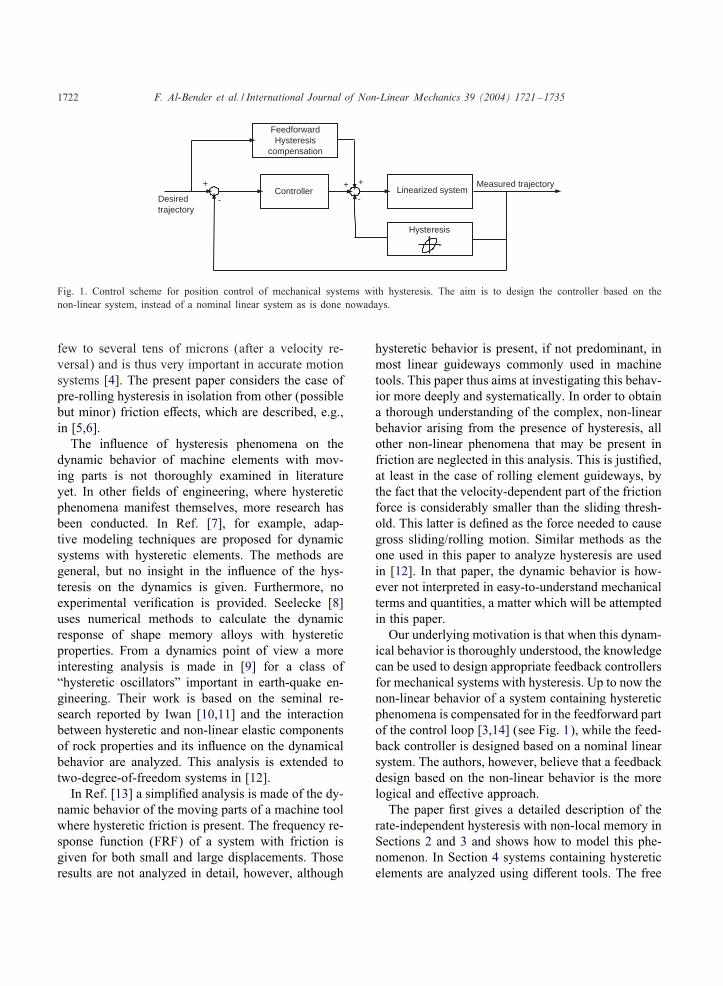
Fig. 1. Control scheme for position control of mechanical systems with hysteresis. The aim is to design the controller based on thenon-linear system, instead of a nominal linear system as is done nowadays.

few to several tens of microns (after a velocity re-versal) and is thus very important in accurate motionsystems [4]. The present paper considers the case ofpre-rolling hysteresis in isolation from other (possiblebut minor) friction e=ects, which are described, e.g.,in [5,6].The inHuence of hysteresis phenomena on the

dynamic behavior of machine elements with mov-ing parts is not thoroughly examined in literatureyet. In other Ields of engineering, where hystereticphenomena manifest themselves, more research hasbeen conducted. In Ref. [7], for example, adap-tive modeling techniques are proposed for dynamicsystems with hysteretic elements. The methods aregeneral, but no insight in the inHuence of the hys-teresis on the dynamics is given. Furthermore, noexperimental veriIcation is provided. Seelecke [8]uses numerical methods to calculate the dynamicresponse of shape memory alloys with hystereticproperties. From a dynamics point of view a moreinteresting analysis is made in [9] for a class of“hysteretic oscillators” important in earth-quake en-gineering. Their work is based on the seminal re-search reported by Iwan [10,11] and the interactionbetween hysteretic and non-linear elastic componentsof rock properties and its inHuence on the dynamicalbehavior are analyzed. This analysis is extended totwo-degree-of-freedom systems in [12].In Ref. [13] a simpliIed analysis is made of the dy-

namic behavior of the moving parts of a machine toolwhere hysteretic friction is present. The frequency re-sponse function (FRF) of a system with friction isgiven for both small and large displacements. Thoseresults are not analyzed in detail, however, although

hysteretic behavior is present, if not predominant, inmost linear guideways commonly used in machinetools. This paper thus aims at investigating this behav-ior more deeply and systematically. In order to obtaina thorough understanding of the complex, non-linearbehavior arising from the presence of hysteresis, allother non-linear phenomena that may be present infriction are neglected in this analysis. This is justiIed,at least in the case of rolling element guideways, bythe fact that the velocity-dependent part of the frictionforce is considerably smaller than the sliding thresh-old. This latter is deIned as the force needed to causegross sliding/rolling motion. Similar methods as theone used in this paper to analyze hysteresis are usedin [12]. In that paper, the dynamic behavior is how-ever not interpreted in easy-to-understand mechanicalterms and quantities, a matter which will be attemptedin this paper.Our underlying motivation is that when this dynam-

ical behavior is thoroughly understood, the knowledgecan be used to design appropriate feedback controllersfor mechanical systems with hysteresis. Up to now thenon-linear behavior of a system containing hystereticphenomena is compensated for in the feedforward partof the control loop [3,14] (see Fig. 1), while the feed-back controller is designed based on a nominal linearsystem. The authors, however, believe that a feedbackdesign based on the non-linear behavior is the morelogical and e=ective approach.The paper Irst gives a detailed description of the

rate-independent hysteresis with non-local memory inSections 2 and 3 and shows how to model this phe-nomenon. In Section 4 systems containing hystereticelements are analyzed using di=erent tools. The free

F. Al-Bender et al. / International Journal of Non-Linear Mechanics 39 (2004) 1721–1735 1723

response of a system is deduced by an analytic so-lution and the more diLcult problem of forced re-sponse is discussed and treated by using the approxi-mate describing function approach. The results of thisapproximation are evaluated by comparisons with di-rect simulation, and the general behavior of the forcedsystem is discussed. Finally, Section 5 draws someappropriate conclusions to be taken up for furtherexperimental validation.

2. Hysteresis in a nutshell

In this paper, we are interested in the “rate-independent hysteresis” of the friction behavior be-tween two bodies which move relative to one another,(regarding other friction characteristics as secondary).The Concise Oxford dictionary gives a general deIni-tion of hysteresis as “the lagging after of e=ect whencause varies in amount etc., especially of magneticinduction behind magnetizing force”. This “laggingbehind” phenomenon, which occurs in many otherphysical phenomena such as surface adsorption, op-tics, etc., should not be confused with the “time lag”that is observed, e.g., in the displacement–veloc-ity relation of a linear mass-damper-spring system.Verstroni and Noori [15] tersely sum up what is un-derstood by hysteresis by: “...a system is said to beendowed with hysteresis if there is a lag in the arrivalof the output with respect to the input, or if outputdepends, in a rate-independent way, on the history ofthe input”. The dependence on the history of the inputmanifests itself in the “non-local memory” charac-ter of hysteresis [16]. Thus, while rate independencerelatively eases the treatment of the problem, thedependence on the history makes it very diLcult toobtain analytically tractable formulations.

3. Description and modeling of rate-independenthysteresis with non-local memory

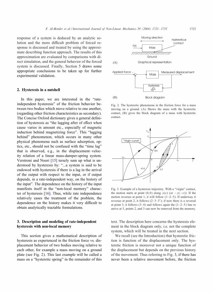
This section gives a mathematical description ofhysteresis as experienced in the friction force vs. dis-placement behavior of two bodies moving relative toeach other, for example a mass moving on a groundplate (see Fig. 2). This last example will be called amass on a “hysteretic spring” in the remainder of this

(A)

(B)

Fig. 2. The hysteretic phenomena in the friction force for a massmoving on a ground. (A) Shows the mass with the hystereticcontact, (B) gives the block diagram of a mass with hystereticcontact.

Fig. 3. Example of a hysteresis trajectory. With a “virgin” contact,the motion starts at point (0; 0) along y(x) (or −y(−x)). If themotion reverses at point 1, it will follow (1–2–5). If underway itreverses at point 2, it follows (2–3–3′); if now there is a reversalat point 3, it follows (3–4) and follows again the (1–2–5) line toarrive at 5, points 2, and 3 can now be removed from the memory.

text. The description here concerns the hysteresis ele-ment in the block diagram only, i.e. not the completesystem, which will be treated in the next section.We recall (see the Introduction) that hysteretic fric-

tion is function of the displacement only. The hys-teretic friction is moreover not a unique function ofthe displacement but depends on the previous historyof the movement. Thus referring to Fig. 3, if there hasnever been a relative movement before, the friction


force follows a virgin curve f(x).

Rule I :{Ffric = f(x) with f(x) =

{y(x) if x¿ 0;

−y(−x) if x6 0:

Usually y(x) has the following properties: y(0) = 0;y′(0)¿ 0 and y′′(x)6 0 (where the primes indicatederivation of the function with respect to its argu-ment). The Irst two properties are universal, while thethird implies that the hysteretic function is “dissipa-tive” for all displacements.If the motion direction changes at x = xm (see

Fig. 3) the friction force becomes:

Rule II :Ffric = Fm + 2f

(x − xm

2

)

Fm = Ffric(xm) calculated with the formula

for Ffric before the reversal:

If the movement reverses again, before x = −xm, thesame reversal Rule II is used for the friction force. If,on the contrary, the direction of movement at x=−xmhas not reversed, the friction force follows Rule Iagain. Thus, when |x| becomes larger than the maxi-mum of the absolute value of any reversal point, RuleI describes the friction force. If |x| is smaller than thisvalue, the friction force is calculated from Rule II us-ing for (Fm; xm) the values of the last reversal point.When “an internal loop is closed” (see for examplethe hatched part in Fig. 3) the two last reversal pointsare not needed anymore, and are thus “forgotten”, andthe curve based on the third last reversal point is fol-lowed. This is called the wiping out e=ect of hystereticbehavior [16]. Based on these rules, the resulting fric-tion force can be calculated for any input motion tra-jectory of the body. This kind of hysteresis is called“hysteresis with non-local memory”, since every ve-locity reversal has to be remembered until an internalloop is closed. The rules (I & II) describing this kindof hysteresis are called “Masing Rules” [17,18]. Thephysics behind this phenomenon can be understoodby imagining friction as asperity adhesion where theasperities Irst deform elastically and then plasticallybefore slip occurs [2]. Experiments [3,19] conIrm therate independent, i.e. frequency independent, characterof this type of friction. Similar phenomena are treated

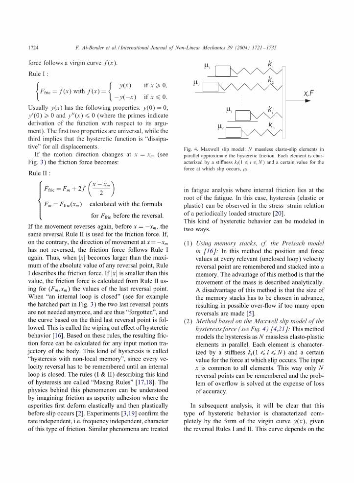
Fig. 4. Maxwell slip model: N massless elasto-slip elements inparallel approximate the hysteretic friction. Each element is char-acterized by a sti=ness ki(16 i6N ) and a certain value for theforce at which slip occurs, �i .

in fatigue analysis where internal friction lies at theroot of the fatigue. In this case, hysteresis (elastic orplastic) can be observed in the stress–strain relationof a periodically loaded structure [20].This kind of hysteretic behavior can be modeled intwo ways.

(1) Using memory stacks, cf. the Preisach modelin [16]: In this method the position and forcevalues at every relevant (unclosed loop) velocityreversal point are remembered and stacked into amemory. The advantage of this method is that themovement of the mass is described analytically.A disadvantage of this method is that the size ofthe memory stacks has to be chosen in advance,resulting in possible over-How if too many openreversals are made [5].

(2) Method based on the Maxwell slip model of thehysteresis force (see Fig. 4) [4,21]: This methodmodels the hysteresis as N massless elasto-plasticelements in parallel. Each element is character-ized by a sti=ness ki(16 i6N ) and a certainvalue for the force at which slip occurs. The inputx is common to all elements. This way only Nreversal points can be remembered and the prob-lem of overHow is solved at the expense of lossof accuracy.

In subsequent analysis, it will be clear that thistype of hysteretic behavior is characterized com-pletely by the form of the virgin curve y(x), giventhe reversal Rules I and II. This curve depends on the


properties (area, roughness, etc.) of the contact sur-faces, the materials used, the temperature, the lubrica-tion, etc. A theoretical derivation of this curve basedon these properties (which hitherto is practically im-possible) is out of the scope of this paper and is ma-terial for detailed tribologic studies. In this paper, theformulas used for the virgin curves are based eitheron experimental measurements (when available) oron arbitrarily assumed shapes (for general analysis).

4. Dynamic behavior of a mass on a “hystereticspring”

This section discusses the dynamic behavior of amass that is connected to a Ixed reference framethrough a “hysteretic spring” (see Fig. 2). It is impor-tant to have a thorough understanding of this dynam-ics if the mass is to be position controlled to a veryaccurate level. Since the hysteretic friction force de-pends on the position and the past velocity reversals,the force is described by: 1

Fhysteresis = �(x; his(xim)): (1)

The equation of motion of the system considered isthen:

m Ox + �(x; his(xim)) = F(t): (2)

Since � is not a polynomial non-linearity, there ap-pear to be hardly any general tools in the literatureto analyze the behavior of systems described by suchequations. Because of this, we investigate the systemdescribed by Eq. (2) in two separate cases; Irst theexcitation force term F(t) is set to zero, giving rise tothe free response of the system. Second, the system isanalyzed under excitation with a harmonic force.

4.1. Free response of the system (F(t) = 0)

The free response of the system described by Eq. (2)is considered when it is brought out of its equilibrium.In that case, the equation of motion becomes

m Ox + �(x; his(xim)) = 0; (3)

1 In this formula his(xim) represents whole the history of themovement that is relevant for the future movement, thus all relevantreversal points (xim; F

im).

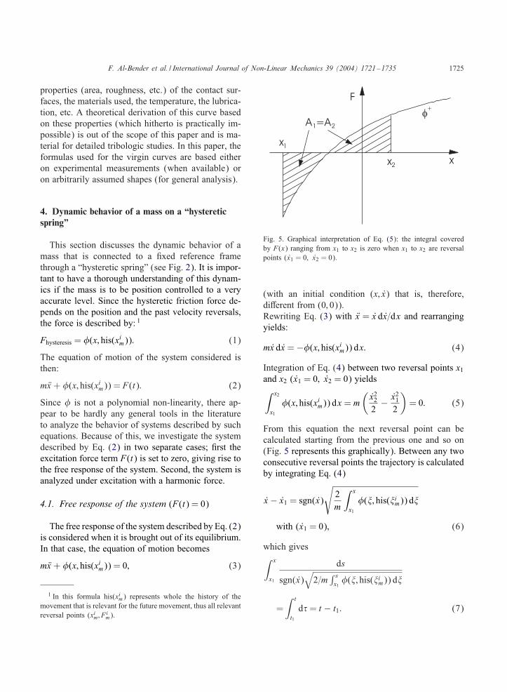
Fig. 5. Graphical interpretation of Eq. (5): the integral coveredby F(x) ranging from x1 to x2 is zero when x1 to x2 are reversalpoints (x1 = 0; x2 = 0).

(with an initial condition (x; x) that is, therefore,di=erent from (0; 0)).Rewriting Eq. (3) with Ox = x dx=dx and rearrangingyields:

mx dx = −�(x; his(xim)) dx: (4)

Integration of Eq. (4) between two reversal points x1and x2 (x1 = 0; x2 = 0) yields∫ x2

x1�(x; his(xim)) dx = m

(x222

− x212

)= 0: (5)

From this equation the next reversal point can becalculated starting from the previous one and so on(Fig. 5 represents this graphically). Between any twoconsecutive reversal points the trajectory is calculatedby integrating Eq. (4)

x − x1 = sgn(x)

√2m

∫ x

x1�(�; his(�im)) d�

with (x1 = 0); (6)

which gives∫ x

x1

ds

sgn(x)√2=m

∫ sx1�(�; his(�im)) d�

=∫ t

t1d�= t − t1: (7)


(A) (B)

(C) (D)

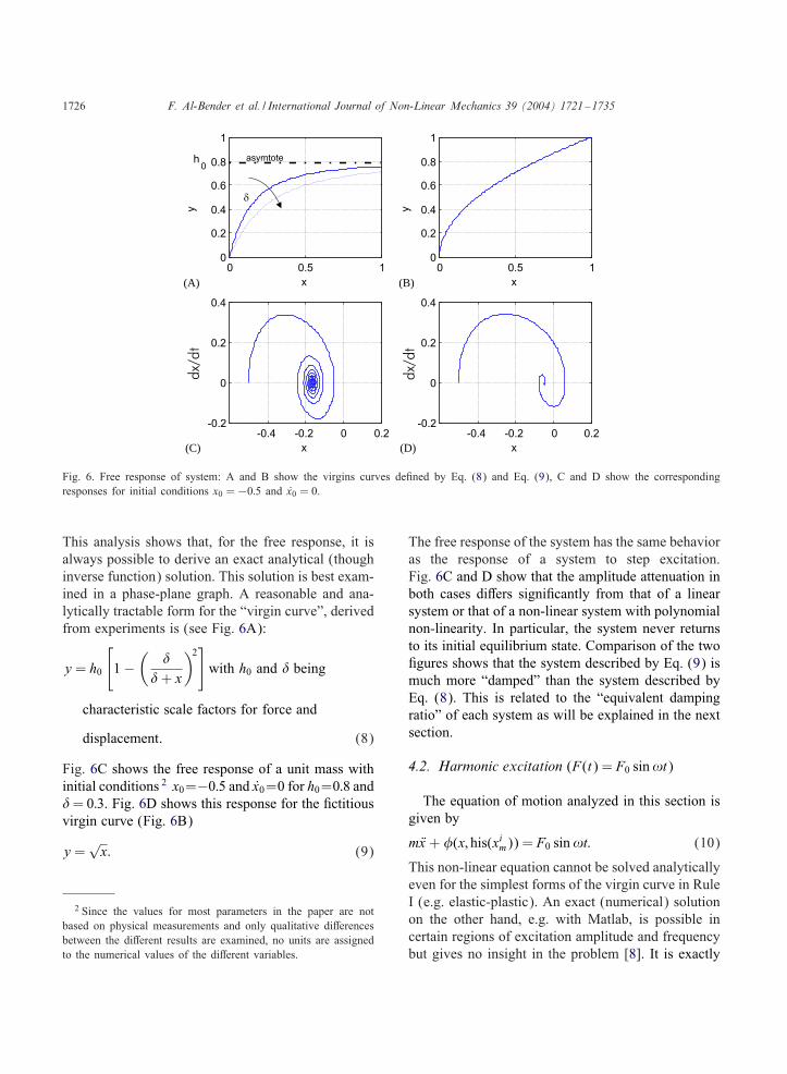
Fig. 6. Free response of system: A and B show the virgins curves deIned by Eq. (8) and Eq. (9), C and D show the correspondingresponses for initial conditions x0 = −0:5 and x0 = 0.

This analysis shows that, for the free response, it isalways possible to derive an exact analytical (thoughinverse function) solution. This solution is best exam-ined in a phase-plane graph. A reasonable and ana-lytically tractable form for the “virgin curve”, derivedfrom experiments is (see Fig. 6A):

y = h0

[1 −

(�

�+ x

)2]with h0 and � being

characteristic scale factors for force and

displacement: (8)

Fig. 6C shows the free response of a unit mass withinitial conditions 2 x0=−0:5 and x0=0 for h0=0:8 and�= 0:3. Fig. 6D shows this response for the Ictitiousvirgin curve (Fig. 6B)

y =√x: (9)

2 Since the values for most parameters in the paper are notbased on physical measurements and only qualitative di=erencesbetween the di=erent results are examined, no units are assignedto the numerical values of the di=erent variables.

The free response of the system has the same behavioras the response of a system to step excitation.Fig. 6C and D show that the amplitude attenuation inboth cases di=ers signiIcantly from that of a linearsystem or that of a non-linear system with polynomialnon-linearity. In particular, the system never returnsto its initial equilibrium state. Comparison of the twoIgures shows that the system described by Eq. (9) ismuch more “damped” than the system described byEq. (8). This is related to the “equivalent dampingratio” of each system as will be explained in the nextsection.

4.2. Harmonic excitation (F(t) = F0 sin!t)

The equation of motion analyzed in this section isgiven by

m Ox + �(x; his(xim)) = F0 sin!t: (10)

This non-linear equation cannot be solved analyticallyeven for the simplest forms of the virgin curve in RuleI (e.g. elastic-plastic). An exact (numerical) solutionon the other hand, e.g. with Matlab, is possible incertain regions of excitation amplitude and frequencybut gives no insight in the problem [8]. It is exactly


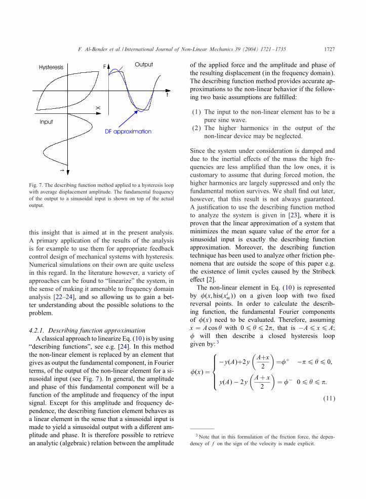
Fig. 7. The describing function method applied to a hysteresis loopwith average displacement amplitude. The fundamental frequencyof the output to a sinusoidal input is shown on top of the actualoutput.

this insight that is aimed at in the present analysis.A primary application of the results of the analysisis for example to use them for appropriate feedbackcontrol design of mechanical systems with hysteresis.Numerical simulations on their own are quite uselessin this regard. In the literature however, a variety ofapproaches can be found to “linearize” the system, inthe sense of making it amenable to frequency domainanalysis [22–24], and so allowing us to gain a bet-ter understanding about the possible solutions to theproblem.

4.2.1. Describing function approximationA classical approach to linearize Eq. (10) is by using

“describing functions”, see e.g. [24]. In this methodthe non-linear element is replaced by an element thatgives as output the fundamental component, in Fourierterms, of the output of the non-linear element for a si-nusoidal input (see Fig. 7). In general, the amplitudeand phase of this fundamental component will be afunction of the amplitude and frequency of the inputsignal. Except for this amplitude and frequency de-pendence, the describing function element behaves asa linear element in the sense that a sinusoidal input ismade to yield a sinusoidal output with a di=erent am-plitude and phase. It is therefore possible to retrievean analytic (algebraic) relation between the amplitude

of the applied force and the amplitude and phase ofthe resulting displacement (in the frequency domain).The describing function method provides accurate ap-proximations to the non-linear behavior if the follow-ing two basic assumptions are fulIlled:

(1) The input to the non-linear element has to be apure sine wave.

(2) The higher harmonics in the output of thenon-linear device may be neglected.

Since the system under consideration is damped anddue to the inertial e=ects of the mass the high fre-quencies are less ampliIed than the low ones, it iscustomary to assume that during forced motion, thehigher harmonics are largely suppressed and only thefundamental motion survives. We shall Ind out later,however, that this result is not always guaranteed.A justiIcation to use the describing function methodto analyze the system is given in [23], where it isproven that the linear approximation of a system thatminimizes the mean square value of the error for asinusoidal input is exactly the describing functionapproximation. Moreover, the describing functiontechnique has been used to analyze other friction phe-nomena that are outside the scope of this paper e.g.the existence of limit cycles caused by the Stribecke=ect [2].The non-linear element in Eq. (10) is represented

by �(x; his(xim)) on a given loop with two Ixedreversal points. In order to calculate the describ-ing function, the fundamental Fourier componentsof �(x) need to be evaluated. Therefore, assumingx = A cos � with 06 �6 2�, that is −A6 x6A;� will then describe a closed hysteresis loopgiven by: 3

�(x) =

−y(A)+2y(A+x2

)=�+ −�6 �6 0;

y(A) − 2y(A+ x2

)= �− 06 �6 �:

(11)

3 Note that in this formulation of the friction force, the depen-dency of f on the sign of the velocity is made explicit.


This yields the fundamental components of thefriction force for a cosinusoidal 4 displacement input

a0 = 0

a1 = − 4�

∫ �

0y

(A2(1 − cos �)

)d�

b1 = − 1�A

{8

∫ A

0

(y(x) − y(A)

2

)dx

}: (12)

The derivation of these formulas can be found inAppendix A.Physical interpretation of the fundamental Fourier

terms is as follows:

(1) The fact that a0 = 0 indicates that there is no DCshift.

(2) The term between {: : :} is equal to the area en-closed by the hysteresis loop of amplitude A.

(3) Since the describing function linearizes the sys-tem in the way described above, it is possible toextract an equivalent sti=ness and damping fromthe fundamental Fourier terms. The equivalentsti=ness of the hysteresis is given by ke = a1=A.The value of ke can be directly calculated fromEq. (12).

(4) The equivalent damping is given by: ce! =−b1=A= loop area=�A2 i.e. the damping force =ce!A = loop area=�A. This amount of energydissipation per cycle does not depend on thevelocity, as in the case of viscous damping, butdepends on the amplitude of the motion. Theloop area per cycle is indeed independent of thevelocity at which the cycle is traversed. In theliterature, this kind of energy dissipation is calledhysteretic damping, solid damping, or structuraldamping. Sometimes this damping is incorpo-rated in the sti=ness term, which is also amplitudedependent. This gives rise to the complex sti=ness(ke+jce) hence our choice of the term “hystereticspring”.

(5) Moreover it is expedient to deIne the equiva-lent damping ratio at resonance �r = ce!=2ke =function(A), which gives a measure of the“damping” capacity of the system. As examples,for the “virgin curve” of Eq. (8) considered inthe previous section, �r → 0 as A → 0; and for

4 This choice makes calculations somewhat easier.

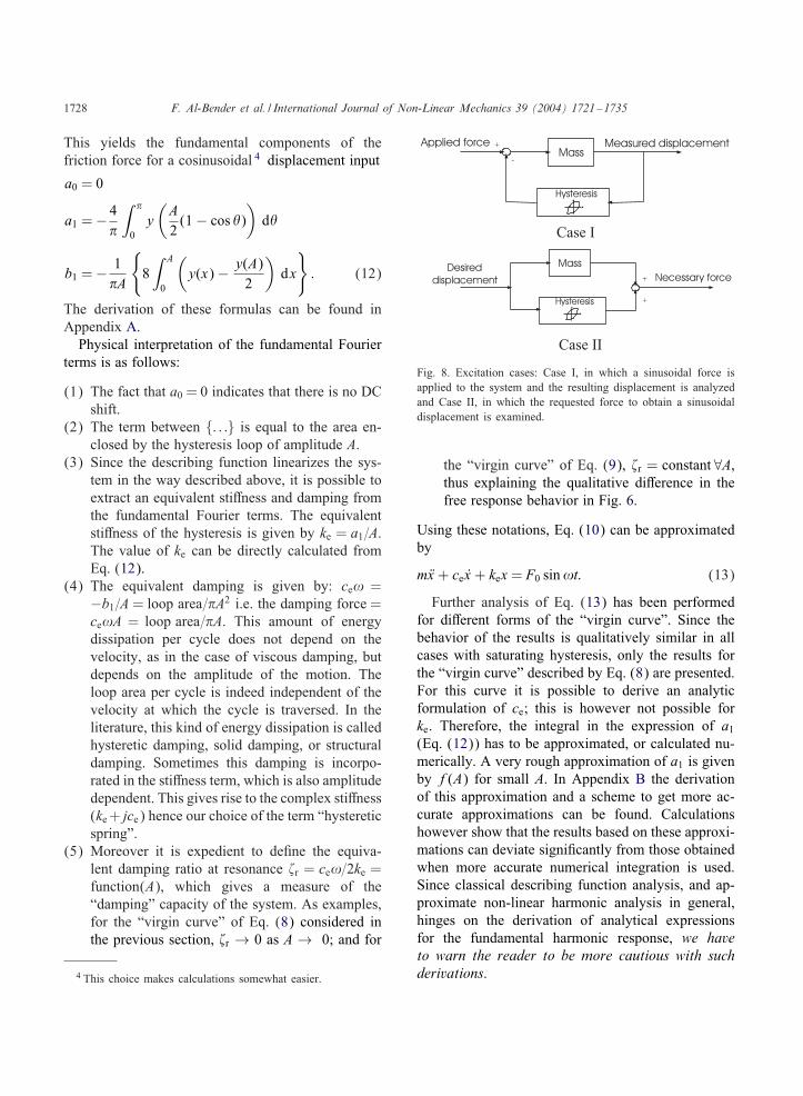
Fig. 8. Excitation cases: Case I, in which a sinusoidal force isapplied to the system and the resulting displacement is analyzedand Case II, in which the requested force to obtain a sinusoidaldisplacement is examined.

the “virgin curve” of Eq. (9), �r = constant ∀A,thus explaining the qualitative di=erence in thefree response behavior in Fig. 6.

Using these notations, Eq. (10) can be approximatedby

m Ox + cex + kex = F0 sin!t: (13)

Further analysis of Eq. (13) has been performedfor di=erent forms of the “virgin curve”. Since thebehavior of the results is qualitatively similar in allcases with saturating hysteresis, only the results forthe “virgin curve” described by Eq. (8) are presented.For this curve it is possible to derive an analyticformulation of ce; this is however not possible forke. Therefore, the integral in the expression of a1(Eq. (12)) has to be approximated, or calculated nu-merically. A very rough approximation of a1 is givenby f(A) for small A. In Appendix B the derivationof this approximation and a scheme to get more ac-curate approximations can be found. Calculationshowever show that the results based on these approxi-mations can deviate signiIcantly from those obtainedwhen more accurate numerical integration is used.Since classical describing function analysis, and ap-proximate non-linear harmonic analysis in general,hinges on the derivation of analytical expressionsfor the fundamental harmonic response, we haveto warn the reader to be more cautious with suchderivations.


(A)

(B)

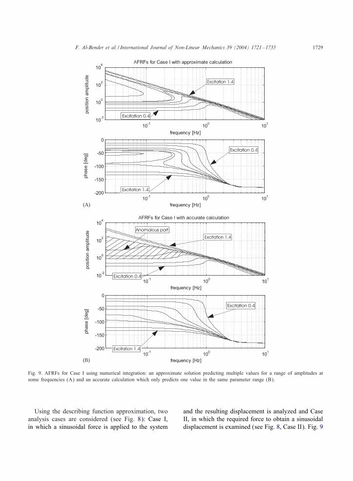
Fig. 9. AFRFs for Case I using numerical integration: an approximate solution predicting multiple values for a range of amplitudes atsome frequencies (A) and an accurate calculation which only predicts one value in the same parameter range (B).

Using the describing function approximation, twoanalysis cases are considered (see Fig. 8): Case I,in which a sinusoidal force is applied to the system

and the resulting displacement is analyzed and CaseII, in which the required force to obtain a sinusoidaldisplacement is examined (see Fig. 8, Case II). Fig. 9


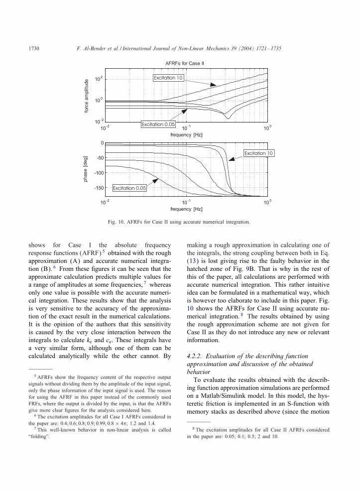
Fig. 10. AFRFs for Case II using accurate numerical integration.

shows for Case I the absolute frequencyresponse functions (AFRF) 5 obtained with the roughapproximation (A) and accurate numerical integra-tion (B). 6 From these Igures it can be seen that theapproximate calculation predicts multiple values fora range of amplitudes at some frequencies, 7 whereasonly one value is possible with the accurate numeri-cal integration. These results show that the analysisis very sensitive to the accuracy of the approxima-tion of the exact result in the numerical calculations.It is the opinion of the authors that this sensitivityis caused by the very close interaction between theintegrals to calculate ke and ce. These integrals havea very similar form, although one of them can becalculated analytically while the other cannot. By

5 AFRFs show the frequency content of the respective outputsignals without dividing them by the amplitude of the input signal,only the phase information of the input signal is used. The reasonfor using the AFRF in this paper instead of the commonly usedFRFs, where the output is divided by the input, is that the AFRFsgive more clear Igures for the analysis considered here.

6 The excitation amplitudes for all Case I AFRFs considered inthe paper are: 0:4; 0:6; 0:8; 0:9; 0:99; 0:8 × 4�; 1.2 and 1.4.

7 This well-known behavior in non-linear analysis is called“folding”.

making a rough approximation in calculating one ofthe integrals, the strong coupling between both in Eq.(13) is lost giving rise to the faulty behavior in thehatched zone of Fig. 9B. That is why in the rest ofthis of the paper, all calculations are performed withaccurate numerical integration. This rather intuitiveidea can be formulated in a mathematical way, whichis however too elaborate to include in this paper. Fig.10 shows the AFRFs for Case II using accurate nu-merical integration. 8 The results obtained by usingthe rough approximation scheme are not given forCase II as they do not introduce any new or relevantinformation.

4.2.2. Evaluation of the describing functionapproximation and discussion of the obtainedbehaviorTo evaluate the results obtained with the describ-

ing function approximation simulations are performedon a Matlab/Simulink model. In this model, the hys-teretic friction is implemented in an S-function withmemory stacks as described above (since the motion

8 The excitation amplitudes for all Case II AFRFs consideredin the paper are: 0.05; 0.1; 0.5; 2 and 10.


(A)

(B)

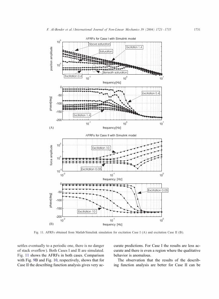
Fig. 11. AFRFs obtained from Matlab/Simulink simulation for excitation Case I (A) and excitation Case II (B).

settles eventually to a periodic one, there is no dangerof stack overHow). Both Cases I and II are simulated.Fig. 11 shows the AFRFs in both cases. Comparisonwith Fig. 9B and Fig. 10, respectively, shows that forCase II the describing function analysis gives very ac-

curate predictions. For Case I the results are less ac-curate and there is even a region where the qualitativebehavior is anomalous.The observation that the results of the describ-

ing function analysis are better for Case II can be


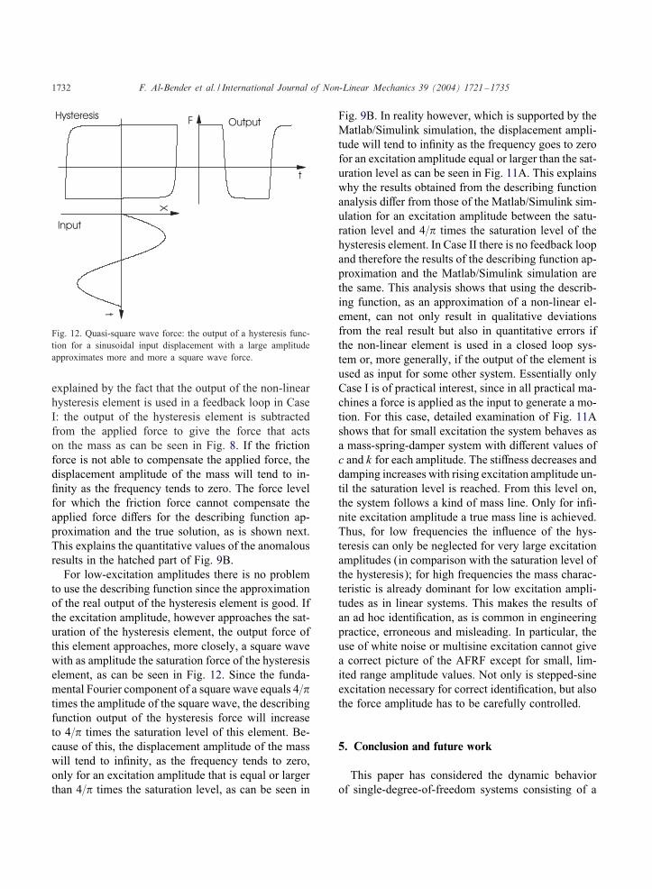
Fig. 12. Quasi-square wave force: the output of a hysteresis func-tion for a sinusoidal input displacement with a large amplitudeapproximates more and more a square wave force.

explained by the fact that the output of the non-linearhysteresis element is used in a feedback loop in CaseI: the output of the hysteresis element is subtractedfrom the applied force to give the force that actson the mass as can be seen in Fig. 8. If the frictionforce is not able to compensate the applied force, thedisplacement amplitude of the mass will tend to in-Inity as the frequency tends to zero. The force levelfor which the friction force cannot compensate theapplied force di=ers for the describing function ap-proximation and the true solution, as is shown next.This explains the quantitative values of the anomalousresults in the hatched part of Fig. 9B.For low-excitation amplitudes there is no problem

to use the describing function since the approximationof the real output of the hysteresis element is good. Ifthe excitation amplitude, however approaches the sat-uration of the hysteresis element, the output force ofthis element approaches, more closely, a square wavewith as amplitude the saturation force of the hysteresiselement, as can be seen in Fig. 12. Since the funda-mental Fourier component of a square wave equals 4=�times the amplitude of the square wave, the describingfunction output of the hysteresis force will increaseto 4=� times the saturation level of this element. Be-cause of this, the displacement amplitude of the masswill tend to inInity, as the frequency tends to zero,only for an excitation amplitude that is equal or largerthan 4=� times the saturation level, as can be seen in

Fig. 9B. In reality however, which is supported by theMatlab/Simulink simulation, the displacement ampli-tude will tend to inInity as the frequency goes to zerofor an excitation amplitude equal or larger than the sat-uration level as can be seen in Fig. 11A. This explainswhy the results obtained from the describing functionanalysis di=er from those of the Matlab/Simulink sim-ulation for an excitation amplitude between the satu-ration level and 4=� times the saturation level of thehysteresis element. In Case II there is no feedback loopand therefore the results of the describing function ap-proximation and the Matlab/Simulink simulation arethe same. This analysis shows that using the describ-ing function, as an approximation of a non-linear el-ement, can not only result in qualitative deviationsfrom the real result but also in quantitative errors ifthe non-linear element is used in a closed loop sys-tem or, more generally, if the output of the element isused as input for some other system. Essentially onlyCase I is of practical interest, since in all practical ma-chines a force is applied as the input to generate a mo-tion. For this case, detailed examination of Fig. 11Ashows that for small excitation the system behaves asa mass-spring-damper system with di=erent values ofc and k for each amplitude. The sti=ness decreases anddamping increases with rising excitation amplitude un-til the saturation level is reached. From this level on,the system follows a kind of mass line. Only for inI-nite excitation amplitude a true mass line is achieved.Thus, for low frequencies the inHuence of the hys-teresis can only be neglected for very large excitationamplitudes (in comparison with the saturation level ofthe hysteresis); for high frequencies the mass charac-teristic is already dominant for low excitation ampli-tudes as in linear systems. This makes the results ofan ad hoc identiIcation, as is common in engineeringpractice, erroneous and misleading. In particular, theuse of white noise or multisine excitation cannot givea correct picture of the AFRF except for small, lim-ited range amplitude values. Not only is stepped-sineexcitation necessary for correct identiIcation, but alsothe force amplitude has to be carefully controlled.

5. Conclusion and future work

This paper has considered the dynamic behaviorof single-degree-of-freedom systems consisting of a


mass on a non-linear “hysteretic spring”. After an ap-propriate description and formulation of the hystere-sis phenomenon, it is shown that an analytic solutioncan be found for the free response problem and thata phase-plane analysis is a suitable tool to investigatethe behavior of such a system. For forced motions,however, an analytic solution is not possible. It is fur-ther shown that the describing function analysis wellapproximates the direct-simulation solution in mostof the amplitude and frequency ranges of harmonicexcitation. However, for some values of the excita-tion amplitude, near saturation, anomalous results areobtained. Therefore, other analysis tools have to bedeveloped. The di=erences in the results obtained bydi=erent analysis methods, for the forced system, indi-cate that care has to be taken when analyzing or iden-tifying highly non-linear systems with approximationmethods. This analysis is of extreme relevance to theproblem of designing appropriate feedback controllersfor mechanical systems with hysteretic friction.Finally, the theoretical analysis of the behavior of

hysteretic friction considered in this paper has beenveriIed experimentally. Results of that investigationwill be presented in another communication, where thepredominance of the hysteretic behavior in pre-rollingfriction becomes clear.

Acknowledgements

This research is sponsored by the Belgian pro-gram of Interuniversity Poles of Attraction by theBelgian State, Prime Minister’s OLce, Science PolicyProgramming (IUAP). The Irst author would like toacknowledge the partial support of the VW-foundationunder Grant no. I/76938. W. Symens was a ResearchAssistant of the Fund for ScientiIc Research—Flan-ders (Belgium) (F.W.O.) during the period this re-search was conducted. The scientiIc responsibility isassumed by its authors.

Appendix A. Calculations to obtain Eq. (12)

The Fourier series of a function f(x) is given by

f(x) =∞∑n=0

an cos (!nx) +∞∑n=1

bn sin (!nx); (A.1)

with

!n = n!0; !0 =2�P;

a0 =12P

∫ P

−P�(x) dx;

an =1P

∫ P

−P�(x) cos(!nx) dx;

bn =1P

∫ P

−P�(x) sin(!nx) dx:

Thus, for the cosinusoidal excitation the fundamentalcomponents of the Fourier series for the friction forceare: 9

a0 =12�

∫ �

−��(A cos �) d�

=12�

[∫ 0

−��+(A cos �) d�+

∫ �

0�−(A cos �) d�

]

=12�

[∫ �

0�+(−A cos �) d �

+∫ �

0�−(A cos �) d�=

]= 0;

a1 =1�

∫ �

−��(A cos �) cos � d �

=12�

[∫ 0

−��+(A cos �) cos � d �

+∫ �

0�−(A cos �) cos � d�

]

=12�

[∫ �

0�+(−A cos �)(−cos �) d �

+∫ �

0�−(A cos �) cos � d �

]

=− 4�

∫ �

0f

(A2(1 − cos �)

)d �;

9 In all the calculations the following change of variable is used:� = � + � on −�6 �6 0.


b1 =1�

∫ �

−�� (A cos �) sin � d�

=12�

[∫ 0

−��+(A cos �) sin � d�

+∫ �

0�−(A cos �) sin � d�

]

=12�

[∫ �

0�+(−A cos �)(−sin �) d�

+∫ �

0�−(A cos �) sin � d�

]

=2�

∫ 1

−1

[f(A) + 2f

(A2(1 − cos �)

)]d(cos �)

=− 1�A

{8

∫ A

0

(f(x) − f(A)

2

)dx

}:

Appendix B. Di+erent approximation formulasfor a1

Table 1 gives some approximations of a1in Eq. (12) based on well-known integration rules.

Table 1Approximations of a1 based on the well-known trapezoidal integration rules and the rules of Simpson

a1 = − 4�

∫ �0 F(�) d� with F(�) = f

(A2(1 − cos �

)cos �

� 0 �=3 �=2 2�=3 �

F(�) 012f

(A4

)0 − 1

2f

(3A4

)−f(A)

Method Approximation of a1

Trapezoidal rule with 3 points f(A)

Trapezoidal rule with 6 points13

[2f(A) +

32f

(3A4

)− 3

2f

(A4

)]

Simpson’s rule with 3 points23f(A)

Simpson’s rule with 6 points13

[f(A) +

32f

(3A4

)− 3

2f

(A4

)]

References

[1] R. Arnell, P. Davies, J. Halling, T. Whomes, Tribology,Macmillan Education, London, 1991.

[2] B. Armstrong-HUelouvry, Control of Machines with Friction,Kluwer Academic Publishers, Dordrecht, 1991.

[3] T. Prajogo, Experimental study of pre-rolling friction formotion-reversal error compensation on machine tool drivesystems, Ph.D. Thesis, Division of Production Engineering,Machine Design and Automation, Katholieke UniversiteitLeuven, 1998.

[4] M. Goldfarb, N. Celanovic, A lumped parameterelectromechanical model for describing the non-linearbehaviour of piezoelectric actuators, Trans. ASME, J. Dyn.Syst. Meas. Control 119 (1979) 478–485.

[5] J. Swevers, F. Al-Bender, C. Ganseman, T. Prajogo, Anintegrated friction model with improved presliding behaviourfor accurate friction compensation, IEEE Trans. Automat.Control 45 (4) (2000) 675–686.

[6] V. Lampaert, J. Swevers, F. Al-Bender, ModiIcations ofthe Leuven integrated friction model structure, IEEE Trans.Automat. Control 47 (4) (2002) 683–687.

[7] A. Smyth, S. Masri, E. Kosmatopoulos, A. Chassiakos, T.Caughey, Development of adaptive modeling techniques fornon-linear hysteretic systems, Int. J. Non-Linear Mech. 37(2002) 1435–1451.

[8] S. Seelecke, Modeling the dynamic behavior of shapememory alloys, Int. J. Non-Linear Mech. 37 (2002)1363–1374.

[9] D. Capecchi, F. Vestroni, Steady-state dynamic analysisof hysteretic systems, J. Eng. Mech. 111 (12) (1985)1515–1531.


[10] W. Iwan, A distributed-element model for hysteresis and itssteady-state dynamic response, Trans. ASME J. Appl. Mech.(1966) 893–900.

[11] W. Iwan, On a class of models for the yielding behavior ofcontinuous and composite systems, Trans. ASME J. Appl.Mech. (1967) 612–617.

[12] R. Masiani, D. Capecchi, F. Vestroni, Resonant and coupledresponse of hysteretic two-degree-of-freedom systems usingharmonic balance method, Int. J. Non-Linear Mech. 37 (2002)1421–1434.

[13] F. Altpeter, Friction modeling, identiIcation and compen-sation, Ph.D. Thesis, UEcole Polytechnique FUederale deLausanne, 1999.

[14] C. Ganseman, Dynamic modeling and identiIcation ofmechanisms with application to industrial robots, Ph.D.Thesis, Division of Production Engineering, Machine designand Automation, Katholieke Universiteit Leuven, 1998.

[15] F. Vestroni, M. Noori, Hysteresis in mechanical systems—modeling and dynamic response, Int. J. Non-Linear Mech.37 (2002) 1261–1262 (Special Issue on Hysteresis).

[16] I. Mayergoyz, Mathematical Models of Hysteresis, Springer,New York, 1991.

[17] G. Masing, Eigenspannungen un verfestigung beim messing,in: Second International Congress for Applied Mechanics,Zurich, 1926, pp. 332–335 (in German).

[18] K. Smith, P. Watson, T. Topper, A stress-strain function forthe fatigue of metals, J. Mater. 5 (4) (1970) 767–778.

[19] S. Futami, A. Furutani, S. Yoshida, Nanometer positioningand its micro-dynamics, Nanotechnology 1 (1) (1990)31–37.

[20] Z. OsUinski (Ed.), Damping of Vibrations, A.A. Balkema,Rotterdam/BrookIeld, 1998.

[21] B. Lazan, Damping of Materials and Members in StructuralMechanics, Pergamon Press, London, 1968.

[22] B. Armstrong, B. Amin, PID Control in the presence of staticfriction: a comparison of algebraic and describing functionanalysis, Automatica 32 (5) (1996) 679–692.

[23] R.H. Macmillan, Non-Linear Control System Analysis,Pergamon Press, Oxford, 1962.

[24] G.J. Taylor, R.G. Brown, Analysis and Design of FeedbackControl Systems, 2nd Edition, McGraw-Hill, New York,1960.

theoretical analysis of the dynamic behavior of hysteresis elements

Documents