thebranchofphysicsthattreatstheactionofforceon statics ...grupen/603/slides/dynamicsi.pdf · •...

Dynamics

The branch of physics that treats the action of force on

bodies in motion or at rest; kinetics, kinematics, and

statics, collectively. — Websters dictionary

Outline

• Conservation of Momentum

• Inertia Tensors - translation and rotation

• Dynamics

– Newton/Euler Dynamics

– Lagrangian Dynamics

– State Space Form - computed torque equation

• Applications:

– simulation;

– control - feedforward compensation;

– analysis - the acceleration ellipsoid.

1 Copyright c©2018 Roderic Grupen

Newton’s Laws

1. a particle will remain in a state of constant rectilinear motionunless acted on by an external force;

2. the time-rate-of-change in the momentum (mv) of the particleis proportional to the externally applied forces, F = d

dt(mv);

and

3. any force imposed on body A by body B is reciprocated by anequal and opposite reaction force on body B by body A.

Conservation of Momentum

Linear:

F =d

dt[mx] = mx

[N] =

[

kg m

sec2

]

Angular:

τ =d

dt

[

Jθ]

= Jθ

[Nm] =

[

kg m2

sec2

]

J is called the mass moment of inertia



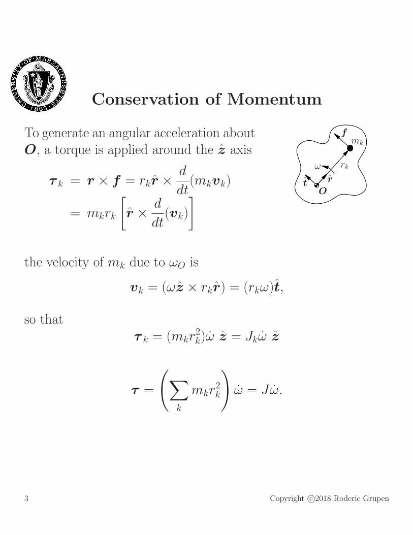
To generate an angular acceleration aboutO, a torque is applied around the z axis

τ k = r × f = rkr ×d

dt(mkvk)

= mkrk

[

r ×d

dt(vk)

]

t r

O

ω rk

fmk

the velocity of mk due to ωO is

vk = (ωz × rkr) = (rkω)t,

so thatτ k = (mkr

2k)ω z = Jkω z

τ =

(

∑

k

mkr2k

)

ω = Jω.



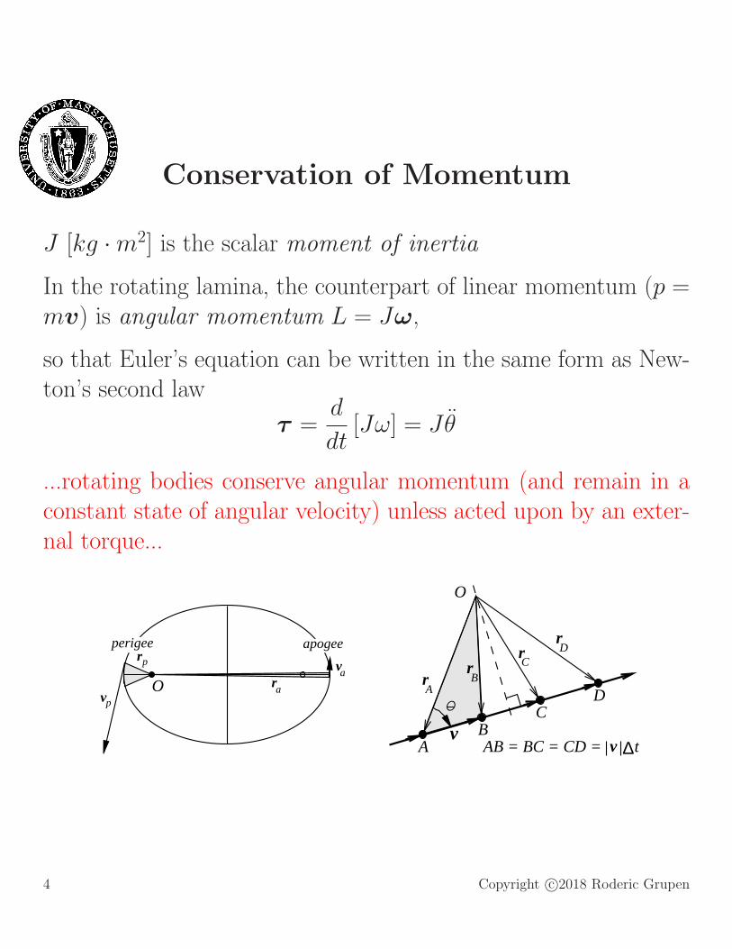
J [kg ·m2] is the scalar moment of inertia

In the rotating lamina, the counterpart of linear momentum (p =mv) is angular momentum L = Jω,

so that Euler’s equation can be written in the same form as New-ton’s second law

τ =d

dt[Jω] = Jθ

...rotating bodies conserve angular momentum (and remain in aconstant state of angular velocity) unless acted upon by an exter-nal torque...

O

BvA

rA

rB

CD

rC

rD

AB = BC = CD = t∆v

O

apogeeperigeerp

raav

pvO


Inertia Tensor

A

y

xz

axisa

A

y

xz

r

r

axisa

jlamina mk

Okt

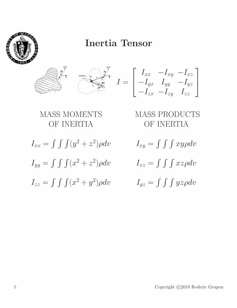
r a I =

Ixx −Ixy −Ixz−Iyx Iyy −Iyz−Izx −Izy Izz

MASS MOMENTS MASS PRODUCTSOF INERTIA OF INERTIA

Ixx =∫ ∫ ∫

(y2 + z2)ρdv Ixy =∫ ∫ ∫

xyρdv

Iyy =∫ ∫ ∫

(x2 + z2)ρdv Ixz =∫ ∫ ∫

xzρdv

Izz =∫ ∫ ∫

(x2 + y2)ρdv Iyz =∫ ∫ ∫

yzρdv


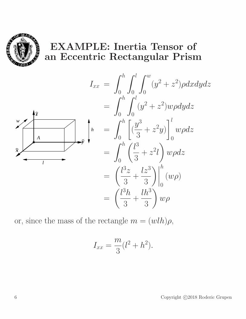
EXAMPLE: Inertia Tensor ofan Eccentric Rectangular Prism

x

y

z

l

h

w

A

Ixx =

∫ h

0

∫ l

0

∫ w

0

(y2 + z2)ρdxdydz

=

∫ h

0

∫ l

0

(y2 + z2)wρdydz

=

∫ h

0

[

(y3

3+ z2y)

]l

0

wρdz

=

∫ h

0

(

l3

3+ z2l

)

wρdz

=

(

l3z

3+

lz3

3

)∣

∣

∣

∣

h

0

(wρ)

=

(

l3h

3+

lh3

3

)

wρ

or, since the mass of the rectangle m = (wlh)ρ,

Ixx =m

3(l2 + h2).


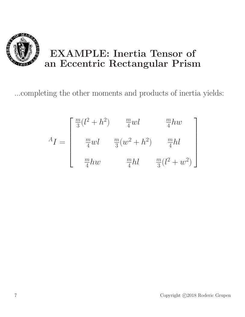
EXAMPLE: Inertia Tensor ofan Eccentric Rectangular Prism

...completing the other moments and products of inertia yields:

AI =

m3(l2 + h2) m

4wl m

4hw

m4wl m

3(w2 + h2) m

4hl

m4hw m

4hl m

3(l2 + w2)


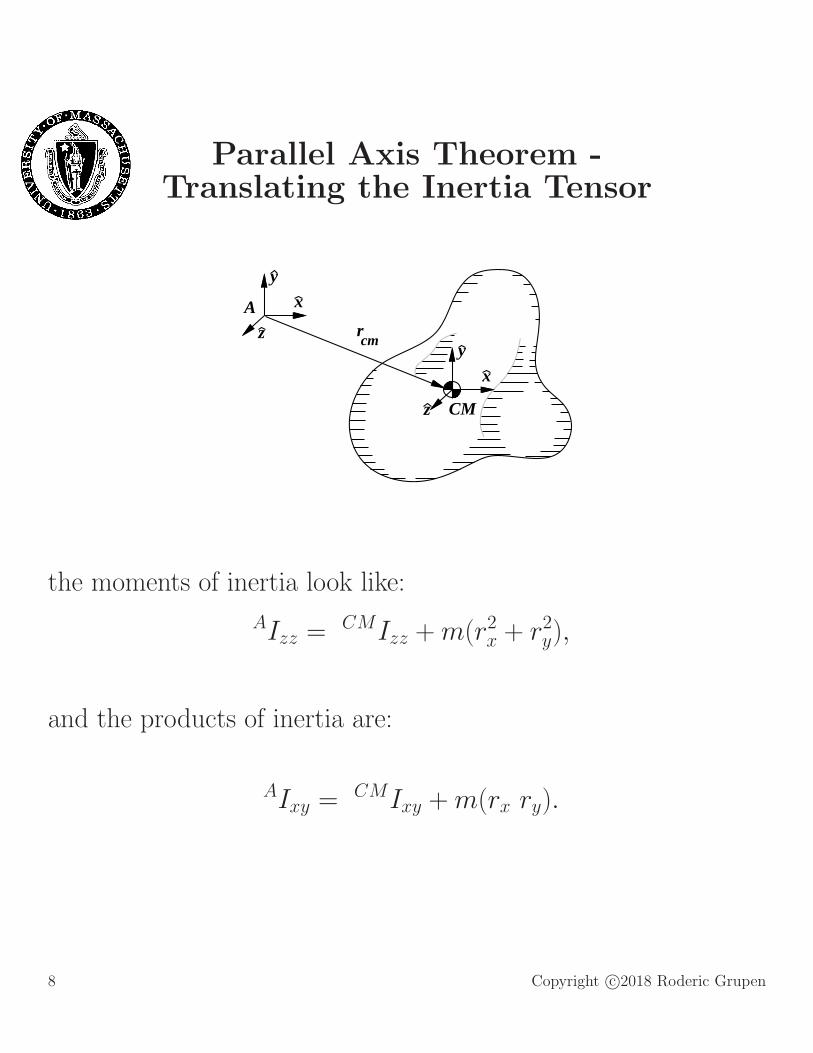
Parallel Axis Theorem -Translating the Inertia Tensor

y

x

z

A

y

x

z

CM

rcm

the moments of inertia look like:

AIzz =CMIzz +m(r2x + r2y),

and the products of inertia are:

AIxy =CMIxy +m(rx ry).


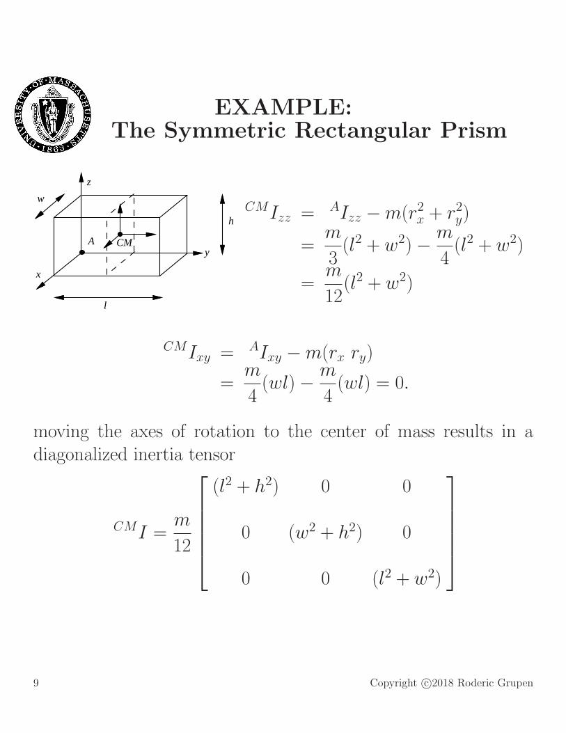
EXAMPLE:The Symmetric Rectangular Prism

x

y

z

l

h

w

A CM

CMIzz = AIzz −m(r2x + r2y)

=m

3(l2 + w2)−

m

4(l2 + w2)

=m

12(l2 + w2)

CMIxy = AIxy −m(rx ry)

=m

4(wl)−

m

4(wl) = 0.

moving the axes of rotation to the center of mass results in adiagonalized inertia tensor

CMI =m

12

(l2 + h2) 0 0

0 (w2 + h2) 0

0 0 (l2 + w2)


Rotating the Inertia Tensor

angular momentum L0 = I0ω about frame 0 in a vector quantitythat is conserved.

we can express it relative to frame 1 as

L1 = 1R0L0

or

I1ω1 = R(I0ω0)

= RI0RTRω0

and therefore,I1 = RI0R

T .


Rotating Coordinate Systems

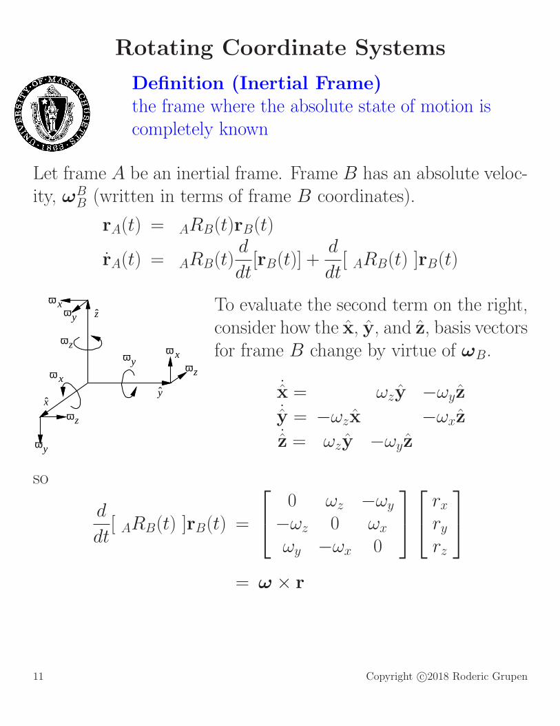
Definition (Inertial Frame)the frame where the absolute state of motion iscompletely known

Let frame A be an inertial frame. Frame B has an absolute veloc-ity, ωB

B (written in terms of frame B coordinates).

rA(t) = ARB(t)rB(t)

rA(t) = ARB(t)d

dt[rB(t)] +

d

dt[ ARB(t) ]rB(t)

yx

z

ω x

ωy

ωz

ωz

ωy

ωz

ω x

ωy

ω x To evaluate the second term on the right,consider how the x, y, and z, basis vectorsfor frame B change by virtue of ωB.

˙x = ωzy −ωyz˙y = −ωzx −ωxz˙z = ωzy −ωyz

so

d

dt[ ARB(t) ]rB(t) =

0 ωz −ωy

−ωz 0 ωx

ωy −ωx 0

rxryrz

= ω × r


Rotating Coordinate Systems

Therefore,

rA(t) = ARB(t)d

dt[rB(t)] +

d

dt[ ARB(t) ]rB(t)

= ARB

[

rB + (ωBB × rB)

]

and, in fact, all vector quantities expressed in local frames thatare moving relative to an inertial frame are differentiated in thisway

d

dt[ARB(t)(·)B] = ARB

[

d

dt(·)B + (ωB × (·)B)

]


Rotating Coordinate Systems:Low Pressure Systems

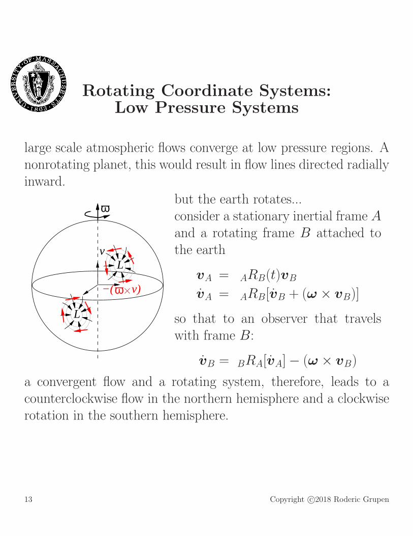
large scale atmospheric flows converge at low pressure regions. Anonrotating planet, this would result in flow lines directed radiallyinward.

−( v)

L

ω

L

ω

v

but the earth rotates...consider a stationary inertial frame Aand a rotating frame B attached tothe earth

vA = ARB(t)vB

vA = ARB[vB + (ω × vB)]

so that to an observer that travelswith frame B:

vB = BRA[vA]− (ω × vB)

a convergent flow and a rotating system, therefore, leads to acounterclockwise flow in the northern hemisphere and a clockwiserotation in the southern hemisphere.


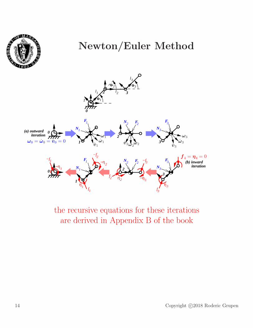
Newton/Euler Method

O1

0

1

l1

O 2

2 l2

O3

3

l3

1

N1

F1

2

F2N2

3

F3

N30(a) outward

iteration

(b) inward iteration

1−η

0

1−f2

−η2

−f

f1

η1

1

N1

F1 3−f

3−ηf2 η2

2

F2N2

η3f3

3

F3

N3

ω1

ω1v1

ω2ω2v2

ω3

ω3v3

ω0 = ω0 = v0 = 0

f 4 = η4 = 0

the recursive equations for these iterationsare derived in Appendix B of the book


Recursive Newton-Euler Equations

Outward Iterations

Angular Velocity: ω

REVOLUTE: i+1ωi+1 = i+1Riiωi + θi+1zi+1

PRISMATIC: i+1ωi+1 = i+1Riiωi

Angular Acceleration: ω

REVOLUTE: i+1ωi+1 = i+1Riiωi + ( i+1Ri

iωi × θi+1zi+1) + θi+1zi+1

PRISMATIC: i+1ωi+1 = i+1Riiωi

Linear Acceleration: v

REVOLUTE: i+1vi+1 = i+1Ri

[

ivi + ( iωi ×ipi+1) + ( iωi ×

iωi ×ipi+1)

]

PRISMATIC: i+1vi+1 = i+1Ri

[

ivi + dixi + 2( iωi × dixi) + ( iωi × dixi)

+ ( iωi ×iωi × dixi)

]

Linear Acceleration (center of mass): vcmi+1vcm,(i+1) = ( i+1ωi+1 ×

i+1pcm)

+ ( i+1ωi+1 ×i+1ωi+1 ×

i+1pcm) + i+1vi+1

Net Force: Fi+1Fi+1 = mi+1

i+1vcm i+1

Net Moment: Ni+1Ni+1 = Ii+1

i+1ωi+1 + ( i+1ωi+1 × Ii+1i+1ωi+1)

Inward Iterations

Inter-Link Forces:ifi =

iFi + iRi+1i+1fi+1

Inter-Link Moments:iηi =

iNi + iRi+1i+1ηi+1 + ( ipcm × iFi)

+ ( ipi+1 × iRi+1i+1fi+1)


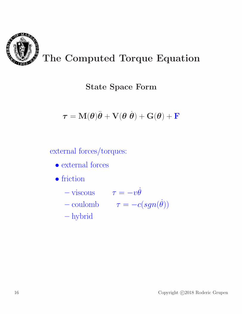
The Computed Torque Equation

State Space Form

τ = M(θ)θ +V(θ θ) +G(θ) + F

external forces/torques:

• external forces

• friction

– viscous τ = −vθ

– coulomb τ = −c(sgn(θ))

– hybrid


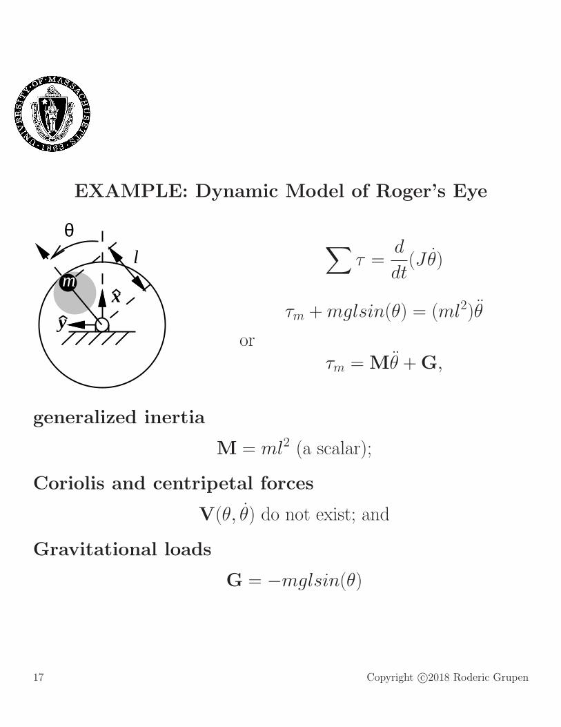
EXAMPLE: Dynamic Model of Roger’s Eye

xy

θl

m

∑

τ =d

dt(Jθ)

τm +mglsin(θ) = (ml2)θ

orτm = Mθ +G,

generalized inertia

M = ml2 (a scalar);

Coriolis and centripetal forces

V(θ, θ) do not exist; and

Gravitational loads

G = −mglsin(θ)


EXAMPLE: Dynamic Model of Roger’s Arm

l1

l2

01

y2

x2

y0

y1 x1

x0

20y3

x3m2

m1

M(θ) =

[

m2l22 + 2m2l1l2c2 + (m1 +m2)l

21 m2l

22 +m2l1l2c2

m2l22 +m2l1l2c2 m2l

22

]

V(θ, θ) =

[

−m2l1l2s2(θ22 + 2θ1θ2)

m2l1l2s2θ21

]

Nm

G(θ) =

[

−(m1 +m2)l1s1g −m2l2s12g

−m2l2s12g

]

Nm


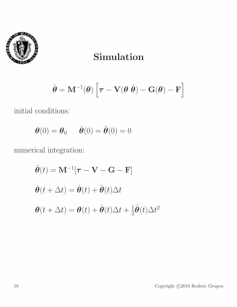
Simulation

θ = M−1(θ)[

τ −V(θ θ)−G(θ)− F]

initial conditions:

θ(0) = θ0 θ(0) = θ(0) = 0

numerical integration:

θ(t) = M−1[τ −V −G− F]

θ(t +∆t) = θ(t) + θ(t)∆t

θ(t +∆t) = θ(t) + θ(t)∆t + 12θ(t)∆t2


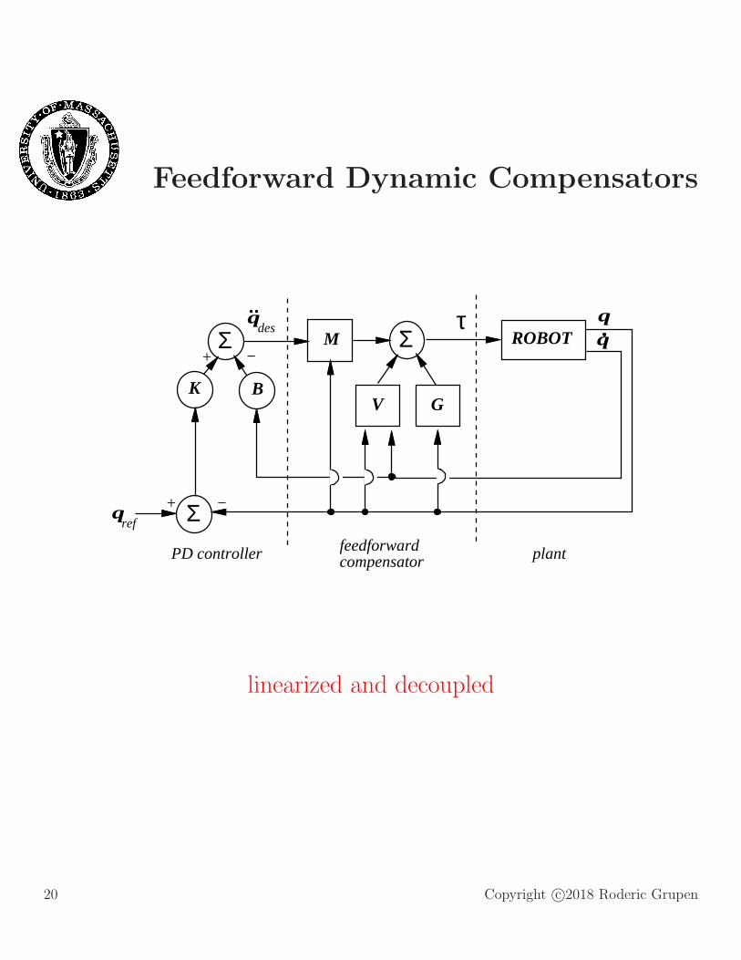
Feedforward Dynamic Compensators

Σ

Σ

Σ ROBOTqq

V G

M

feedforwardcompensator plant

qdes

ref

PD controller

+

+

−

τ

K B

−

q

linearized and decoupled


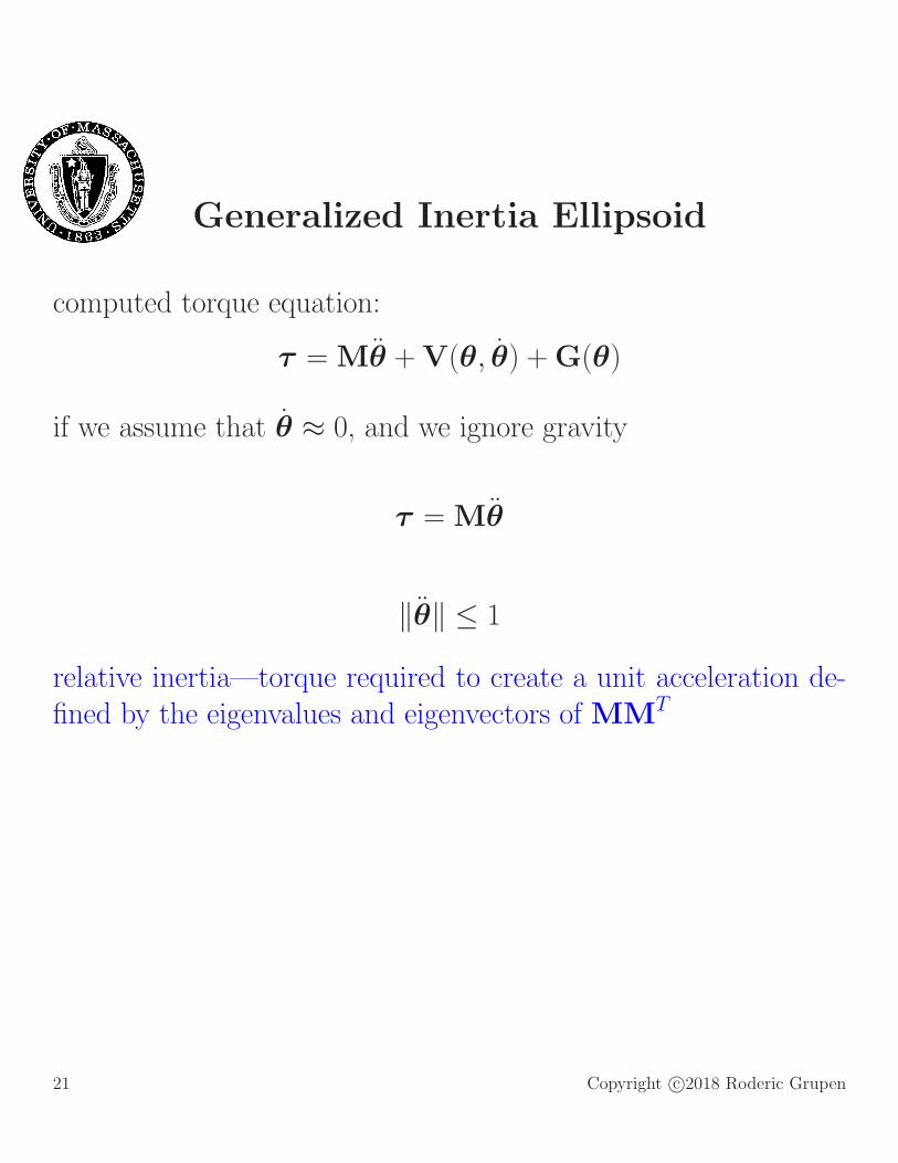
Generalized Inertia Ellipsoid

computed torque equation:

τ = Mθ +V(θ, θ) +G(θ)

if we assume that θ ≈ 0, and we ignore gravity

τ = Mθ

‖θ‖ ≤ 1

relative inertia—torque required to create a unit acceleration de-fined by the eigenvalues and eigenvectors of MMT


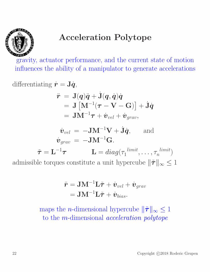
Acceleration Polytope

gravity, actuator performance, and the current state of motioninfluences the ability of a manipulator to generate accelerations

differentiating r = Jq,

r = J(q)q + J(q, q)q

= J[

M−1(τ −V −G)]

+ Jq

= JM−1τ + vvel + vgrav,

vvel = −JM−1V + Jq, and

vgrav = −JM−1G.

τ = L−1τ L = diag(τ limit1 , . . . , τ limit

n )

admissible torques constitute a unit hypercube ‖τ‖∞ ≤ 1

r = JM−1Lτ + vvel + vgrav

= JM−1Lτ + vbias.

maps the n-dimensional hypercube ‖τ‖∞ ≤ 1to the m-dimensional acceleration polytope


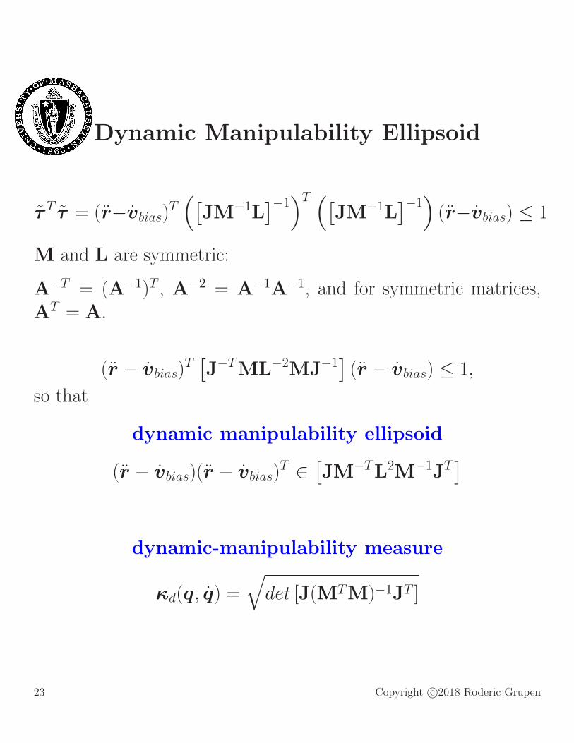
Dynamic Manipulability Ellipsoid

τ T τ = (r−vbias)T(

[

JM−1L]−1)T (

[

JM−1L]−1)

(r−vbias) ≤ 1

M and L are symmetric:

A−T = (A−1)T , A−2 = A−1A−1, and for symmetric matrices,AT = A.

(r − vbias)T[

J−TML−2MJ−1]

(r − vbias) ≤ 1,

so that

dynamic manipulability ellipsoid

(r − vbias)(r − vbias)T ∈

[

JM−TL2M−1JT]

dynamic-manipulability measure

κd(q, q) =√

det [J(MTM)−1JT ]


Conditioning Acceleration

y

x

y

x

x=0.5 m

x=0.3 m

y=−0.265 m y=−0.765 m

m1 = m2 = 0.2 kg, l1 = l2 = 0.25 m, τTτ ≤ 0.005 N 2m2.

black ellipsoids - unbiased dynamic manipulabilitygravity biased dynamic manipulabilitynormalized acceleration polytope with gravity bias


thebranchofphysicsthattreatstheactionofforceon statics ...grupen/603/slides/dynamicsi.pdf · •...

Documents