arX

iv:0

907.

0830

v1 [

astr

o-ph

.CO

] 5

Jul

200

9Astronomy & Astrophysics manuscript no. lsb c© ESO 2018November 8, 2018

The age of blue LSB galaxies

E. I. Vorobyov1,2, Yu. Shchekinov5⋆, and D. Bizyaev3,4, D. Bomans5, R.-J. Dettmar5,

1 The Institute for Computational Astrophysics, Saint Mary’s University, Halifax NS, B3H 3C3, Canada2 Institute of Physics, South Federal University, Stachki 194, Rostov-on-Don, Russia3 New Mexico State University/APO, Sunspot, NM, 88349, USA4 Sternberg Astronomical Institute, Universitetsky 13, Moscow, 119992, Russia5 Astronomisches Institut, Ruhr-Universitat Bochum, Bochum, Germany

ABSTRACT

Context. Low metallicities, large gas-to-star mass ratios, and blue colors of most low surface brightness (LSB) galaxiesimply that these systems may be younger than their high surface brightness counterparts.Aims. We seek to find observational signatures that can help to constrain the age of blue LSB galaxies.Methods. We use numerical hydrodynamic modelling to study the long-term (∼ 13 Gyr) dynamical and chemicalevolution of blue LSB galaxies adopting a sporadic scenario for star formation. Our model galaxy consists of a thin gasdisk, stellar disk with a developed spiral structure and spherical dark matter halo. Our models utilize various rates ofstar formation and different shapes of the initial mass function (IMF). We complement hydrodynamic modelling withpopulation synthesis modelling to produce the integrated B − V colors and Hα equivalent widths.Results. We find that the mean oxygen abundances, B − V colors, Hα equivalent widths, and the radial fluctuationsin the oxygen abundance, when considered altogether, can be used to constrain the age of blue LSB galaxies if someindependent knowledge of the IMF is available. Our modelling strongly suggests the existence of a minimum age forblue LSB galaxies. Model B − V colors and mean oxygen abundances set a tentative minimum age at 1.5–3.0 Gyr,whereas model Hα equivalent widths suggest a larger value of order 5–6 Gyr. The latter value may decrease somewhat,if blue LSB galaxies host IMFs with a truncated upper mass limit. We found no firm evidence that the age of blue LSBgalaxies is significantly smaller than 13 Gyr.Conclusions. The age of blue LSB galaxies may vary between 1.5–6 Gyr and 13 Gyr, depending on the physical conditionsin the disk that control the form of the IMF and the rate of star formation. A failure to observationally detect largeradial fluctuations in the oxygen abundance of order 0.5–1.0 dex, which, according to our modelling, are characteristicof (1-2)-Gyr-old galaxies, will argue in favour of the more evolved nature of blue LSB galaxies.

Key words. ISM:galaxies – galaxies:abundances – galaxies:evolution

1. Introduction

Low surface brightness (LSB) galaxies are the galaxieswhose central surface brightness is much fainter than theFreeman value µB = 21.65 ± 0.30 mag arcsec−2. Thesegalaxies are thought to represent a significant fraction ofthe galaxy number density in the universe (McGaugh et al.,1995; O’Neil & Bothun, 2000; Trachternach et al., 2006).LSB galaxies show a wide spread of colours rangingfrom red (B − V ≃ 1.7) to very blue (B − V ≃0.2) (O’Neil et al., 1997), but the most common typeseems to be blue LSB galaxies: late-type, disk dom-inated spirals with central surface brightness µB >∼23 mag arcsec−2 and colors lying in the range (B −V ) = 0.3 − 0.7. These blue LSB galaxies are among themost gas-rich (up to 50% of the total baryonic mass)and metal-deficient (about 5%-20% of the solar metallic-ity) galaxies (McGaugh, 1994; Ronnback & Bergvall, 1995;McGaugh & Blok, 1997; de Blok & van der Hulst, 1998;Kuzio de Narray et al., 2004).

Low metallicities and large gas-to-star mass ratios maybe interpreted in various ways. For instance, blue LSB

Send offprint requests to: E. I. Vorobyov⋆ on leave from Department of Physics, South Federal

University, and Special Astrophysical Observatory

galaxies may have formed recently, at redshifts close toz = 0. However, this can confront the hierarchical scenarioof large-scale structure formation, within which low-massgalaxies form first at redshifts close to the onset of the reion-ization epoch, z ∼ 10. Therefore, it is more likely that blueLSB galaxies have formed at large z but have had a delayedonset of major star formation epoch. In this case, a conflictwith the hierarchical structure formation is relaxed. Indeed,blue LSB galaxies show a wide range of masses with an ex-cess of dwarf systems with luminosities of order 107−108L⊙

(Sprayberry et al., 1997). Such dwarf systems are knownto have a younger mean stellar age than their more mas-sive counterparts – a phenomenon known as ‘downsizing’(e.g. Thomas et al., 2005). Another possible interpretationof the apparent unevolved nature of blue LSBs is that theydo not form late, nor have a delayed onset of star formation,but simply evolve slower than their high surface brightnesscounterparts (e.g. van den Hoek et al., 2000).

There have been many efforts to infer the age ofblue LSB galaxies from the properties of stellar popula-tion. Broadband photometric studies, complemented by Hαemission line data and synthetic stellar population codemodeling, predict quite a wide range for the ages of blueLSB galaxies: from 1-2 Gyr (Zackrisson et al., 2005) to 7-9 Gyr (Padoan et al., 1997; Jimenez et al., 1998). Rather

2 Vorobyov et al.: Age of blue LSB galaxies

young ages of blue LSB galaxies (< 5 Gyr) follow alsofrom their (V − I) colors and HI content (Schombert et al.,2001). The comparison of measured spectral energy distri-butions in a sample of LSB galaxies with the synthetic spec-tra (derived assuming an exponentially declining SFR) byHaberzettl et al. (2005) suggests the ages of the dominantstellar population between 2 and 5 Gyr.

In this paper, we perform numerical hydrodynamicmodelling of the dynamical, chemical, and photometricevolution of blue LSB galaxies with the purpose to con-strain their typical range of ages. The cornerstone sup-position of our modelling, motivated by observational evi-dence, is a sporadic nature of star formation in blue LSBgalaxies. Indeed, McGaugh (1994), de Blok et al. (1995),Gerretsen & de Blok (1999), and others argue that the pri-mary cause for the blue colors is the young age of the dom-inant stellar population. This can take the form of younglocal bursts of star formation superimposed (or not) ona continuous low-rate star formation. Available Hα im-ages of LSB galaxies (see e.g. McGaugh & Bothun, 1994;McGaugh et al., 1995; Auld et al., 2006) appear to sup-port this so-called sporadic star formation scenario. Currentstar formation is localized to a handful of compact regions.There is little or no diffuse Hα emission coming from therest of the galactic disk. Randomly distributed star forma-tion sites, along with inefficient spatial stirring of heavy el-ements, give rise to radial fluctuations in the oxygen abun-dance on spatial scales of order 1 − 2 kpc. The resultedfluctuation spectrum is age-sensitive and can be potentiallyused to set order-of-magnitude constraints on the age ofblue LSB galaxies. However, the age prediction may be con-siderably improved by using the mean oxygen abundancesand Hα equivalent widths provided that some independentknowledge of the initial mass function is available.

The paper is organized as follows. In the next Sectionwe discuss qualitatively the processes that mix heavy ele-ments in disks of LSB galaxies. Section 3 details our the-oretical model, while Section 4 describes our observations.In Sections 5 and 6 we discuss our numerical results, andSection 7 presents main conclusions.

2. Mixing of heavy elements in LSB disks

In high surface brightness (HSB) galaxies mixing of heavyelements is provided by multiple shock waves from super-nova explosions. It requires approximately 100 Myr to ho-mogenize heavy elements in the warm neutral interstel-lar medium of HSB galaxies (de Avillez & MacLow, 2002).LSB galaxies, on the other hand, are characterized by thestar formation rate (∼ 0.1M⊙ yr−1) that is almost two or-ders of magnitude lower than the Milky Way value, ≈ 5M⊙

yr−1. Consequently, the frequency of shock waves in theinterstellar medium of LSB galaxies and the correspond-ing volume filling factor occupied by the shock processedgas can be as small as Ψsh

<∼ (200 Myr)−1 and fsh <

∼ 0.004,respectively. For comparison, the corresponding values inthe Milky Way are Ψsh ∼ (5 Myr)−1 (Draine & Salpeter,1979) and fsh ∼ 0.2 (de Avillez & Breitschwerdt, 2005). Inthese conditions, homogenization of heavy elements in LSBgalaxies may require a considerably longer time scale than100 Myr, a typical value for HSB galaxies. Differential ro-tation of the galactic disk and radial convection driven bythe spiral stellar density waves may in principle be efficientin mixing of heavy elements in LSB galaxies. However, the

time scales for these processes in LSB galaxies are not wellknown and numerical simulations are needed to determinetheir importance. Therefore, the distribution of heavy ele-ments in the disk of an LSB galaxy may be characterizedby radial variations, the typical amplitude of which is ex-pected to diminish with time. It is our purpose to determinewhether these radial abundance fluctuations can be used toconstrain the ages of LSB galaxies.

We note that mixing in the azimuthal direction isstrongly enhanced by differential rotation. Namely, the sizeof a mixing eddy grows with time due to differential ro-tation as ∆x ∼ (uφ)

′

r D1/2t3/2, much faster than due to

hydrodynamic mixing ∆x ∝ t (Scalo & Elmegreen, 2004),where (uφ)

′

r is the radial derivative of the rotation velocity,D is the diffusion coefficient. Differential rotation thereforehomogenizes metals in the azimuthal direction faster thanin the radial one and the radial variations remain for alonger time.

3. Model LSB galaxy

3.1. Initial configuration

LSB galaxies show a wide range of morphological types,ranging from giant spirals to dwarf irregular galaxies, fromearly-type red galaxies to late-type blue ones. In this pa-per we focus on late-type blue LSB galaxies. According tothe observational data (van den Hoek et al., 2000), a typi-cal blue LSB galaxy has a dynamical mass of order 1010 M⊙

and HI mass of order 2 × 109 M⊙. We closely follow theseestimates when constructing our model galaxy. Our modelLSB galaxy consists of a thin gas disk, which evolves in theexternal gravitational potential of both the spherical darkmatter halo and extended stellar disk. LSB galaxies oftenfeature a few ill-defined spiral arms. Therefore, we assumethat our model stellar disk has developed a two-armed spi-ral structure. Below, we provide a more detailed explana-tion for each of the constituents of our model galaxy.

The velocity field of most LSB galaxies is betterfitted by dark matter models described by a modi-fied isothermal sphere rather than by a NFW profile(Kuzio de Naray et al., 2006). Therefore, the spherical darkmatter halo in our model is modelled by a radial densityprofile described by the modified isothermal sphere

ρh =ρh0

(1 + r/rh)2, (1)

where ρh0 = 6.0× 10−3 M⊙ pc−3 and rh = 5.7 kpc are thecentral volume density and characteristic scale length of thedark matter halo, respectively, and r is the radial distance.The adopted values of ρh0 and rh are similar to those ob-tained by Kuzio de Naray et al. (2006) for UGC 5750. Thedark matter halo mass in the inner 15 kpc is approximately2.0×1010 M⊙. The radial gravity force (per unit mass) dueto the spherical dark matter halo in the plane of the diskcan be written as

∂Φh

∂r= 4πGρh0rh [r/rh − arctan(r/rh)]

(rhr

)2

. (2)

The stellar component of our model galaxy consists oftwo parts – an axisymmetric stellar disk and a two-armedspiral pattern. The former is described by a radially declin-ing exponential profile

Σst = Σs0 exp(−r/rs), (3)

Vorobyov et al.: Age of blue LSB galaxies 3

where Σs0 = 30 M⊙ pc−2 is the central stellar surface den-sity and rs = 4 kpc is the radial scale length of the stellardisk. The adopted value for rs is typical for blue LSB galax-ies (de Blok et al., 1995). We note that our model stellardisk serves as a proxy to the real stellar disk that is expectedto form during the evolution of our model galaxy. The massof the stellar disk in the inner 15 kpc is Ms = 2.6×109 M⊙.For numerical purposes, the gravitational potential of theaxisymmetric thin stellar disk in the plane of the disk iscalculated as

Φst(r, z = 0) = −πGΣs0r [I0(y)K1(y)− I1(y)K0(y)] , (4)

where In and Kn are modified Bessel functions of the firstand second kinds, respectively, and y ≡ r/(2rs).

The non-axisymmetric gravitational potential of stellarspiral arms is described in polar coordinates (r, φ) by a run-ning density wave (see e.g. Vorobyov & Shchekinov, 2005)

Φsp(r, φ) = −C(r) cos [m(cot(i) ln(r/rsp) + φ− Ωspt)] , (5)

where C(r) is the radially varying amplitude, i is the pitchangle, rsp is the characteristic radius of the spiral at φ = 0,m = 2 is the number of spiral arms, and Ωsp is the angularvelocity of the spiral pattern. In the following we adoptrsp = 6 kpc and Ωsp = 5.5 km s−1 kpc. The pitch angle isset to 25, typical for the late-type spiral galaxies.

The amplitude C(r) of the spiral stellar gravitationalpotential Φsp determines the response of the gas and con-sequently the appearance of a spiral pattern in the gasdisk. We adopt the following expression for the amplitudeC(r) = C0(r)

α(r). Here, C0(r) is a linear function of radiuswhich has a value of 0 at r = 0 kpc and equals 1.8× 10−3

(in dimensionless units) at r = 17 kpc. The amplitude isset to zero at the galactic center to ensure that the gravi-tational potential of the stellar spiral density wave dimin-ishes at small galactocentric distances. Otherwise, even asmall-amplitude spiral gravitational potential would pro-duce strong azimuthal gravitational forces near the galacticcenter due to converging radial gridlines in polar coordi-nates, which quickly destroys the gas disk during the nu-merical simulations. The exponent α(r) decreases linearlywith radius r. More specifically, we choose α(r = 0 kpc) =2.3, and α(r = 17 kpc) = 0.6. This specific form of C(r)allows us to produce spiral gravitational potentials with dif-ferent shapes and maximum amplitudes. The resulted ratioβ(r) of the maximum non-axisymmetric gravitational accel-eration due to spiral arms [(∂Φsp/∂r)

2+(r−1 ∂Φsp/∂φ)2]1/2

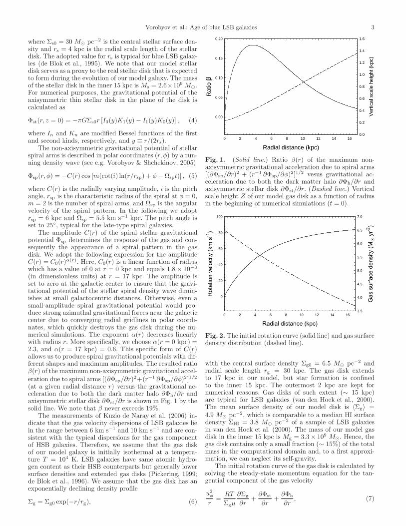
(at a given radial distance r) versus the gravitational ac-celeration due to both the dark matter halo ∂Φh/∂r andaxisymmetric stellar disk ∂Φst/∂r is shown in Fig. 1 by thesolid line. We note that β never exceeds 19%.

The measurements of Kuzio de Naray et al. (2006) in-dicate that the gas velocity dispersions of LSB galaxies liein the range between 6 km s−1 and 10 km s−1 and are con-sistent with the typical dispersions for the gas componentof HSB galaxies. Therefore, we assume that the gas diskof our model galaxy is initially isothermal at a tempera-ture T = 104 K. LSB galaxies have same atomic hydro-gen content as their HSB counterparts but generally lowersurface densities and extended gas disks (Pickering, 1999;de Blok et al., 1996). We assume that the gas disk has anexponentially declining density profile

Σg = Σg0 exp(−r/rg), (6)

Radial distance (kpc)

0 2 4 6 8 10 12 14 16

Rat

io β

0.00

0.05

0.10

0.15

0.20

Ver

tical

sca

le h

eigh

t (kp

c)

0.0

0.2

0.4

0.6

0.8

1.0

1.2

1.4

1.6

Fig. 1. (Solid line.) Ratio β(r) of the maximum non-axisymmetric gravitational acceleration due to spiral arms[(∂Φsp/∂r)

2 + (r−1 ∂Φsp/∂φ)2]1/2 vesus gravitational ac-

celeration due to both the dark matter halo ∂Φh/∂r andaxisymmetric stellar disk ∂Φst/∂r. (Dashed line.) Verticalscale height Z of our model gas disk as a function of radiusin the beginning of numerical simulations (t = 0).

Radial distance (kpc)

0 2 4 6 8 10 12 14 16

Ro

tatio

n v

elo

city (

km

s-1

)

0

20

40

60

80

100

Ga

s s

urf

ace d

en

sity (

M

yr-2

)

3.5

4.0

4.5

5.0

5.5

6.0

6.5

7.0

Fig. 2. The initial rotation curve (solid line) and gas surfacedensity distribution (dashed line).

with the central surface density Σg0 = 6.5 M⊙ pc−2 andradial scale length rg = 30 kpc. The gas disk extendsto 17 kpc in our model, but star formation is confinedto the inner 15 kpc. The outermost 2 kpc are kept fornumerical reasons. Gas disks of such extent (∼ 15 kpc)are typical for LSB galaxies (van den Hoek et al., 2000).The mean surface density of our model disk is 〈Σg〉 =4.9 M⊙ pc−2, which is comparable to a median HI surfacedensity ΣHI = 3.8 M⊙ pc−2 of a sample of LSB galaxiesin van den Hoek et al. (2000). The mass of our model gasdisk in the inner 15 kpc is Mg = 3.3× 109 M⊙. Hence, thegas disk contains only a small fraction (∼ 15%) of the totalmass in the computational domain and, to a first approxi-mation, we can neglect its self-gravity.

The initial rotation curve of the gas disk is calculated bysolving the steady-state momentum equation for the tan-gential component of the gas velocity

u2φ

r=

RT

Σgµ

∂Σg

∂r+

∂Φst

∂r+

∂Φh

∂r, (7)

4 Vorobyov et al.: Age of blue LSB galaxies

Table 1. Main structural properties of our model galaxy

mass scale length central densityStellar disk 2.6× 109 4 30gas disk 3.3× 109 30 6.5halo 2.0× 1010 5.7 6.0× 10−3

All masses are in M⊙, scale lengths in kpc, and densities inM⊙ pc−2 (gas and stellar disks) and M⊙ pc−3 (halo). All

masses are calculated inside 15 kpc radius.

where µ = 1.2 is the mean molecular weight for a gas ofatomic hydrogen (76% by mass) and atomic helium (24%by mass) and R is the universal gas constant. The initialradial gas density profile and rotation curve are shown inFig. 2 by the dashed and solid lines, respectively. It is evi-dent that our model LSB galaxy is characterized by a risingrotation curve with a maximum rotation velocity of approx-imately 80 km s−1, in agreement with the measured shapesof the rotation curve in UGC 5750 and other LSB galaxiesKuzio de Naray et al. (2006). The main properties of ourmodel galaxy are summarized in Table 1.

3.2. Basic equations

We use the thin-disk approximation to compute the long-term evolution of our model LSB galaxy. It is only thegas disk that is dynamically active, while both the stel-lar disk and dark matter halo serve as a source of exter-nal gravitational potential. In the thin-disk approximation,the vertical motions in the gas disk are neglected and thebasic equations of hydrodynamics are integrated in the z-direction from z = −Z(r, φ, t) to z = +Z(r, φ, t) to yieldthe following equations in polar coordinates (r, φ)

∂Σg

∂t+∇p · (vpΣg) = −βRM ΣSFR, (8)

∂sp∂t

+ ∇p · (sp · vp) = −∇pp− Σg∇pΦh

− Σg∇p(Φsp +Φst)− vpβRM ΣSFR, (9)

∂ǫ

∂t+∇p · (vpǫ) = −p(∇ · v) + Γsn + 2Z(Γcr + Γbg)

− 2ZΛ− v2pβRM ΣSFR. (10)

In the above equations, vp = rvr + φvφ is the gas velocityin the disk plane, sp ≡ Σgvp is the momentum per surface

area in the disk plane, ∇p = r∂/∂r + φr−1∂/∂φ is thegradient along the planar coordinates of the disk, p is thevertically integrated gas pressure, ǫ is the internal energyper surface area, and Z is the vertical scale height of the gasdisk. The basic equations of hydrodynamics are modified toinclude the effect of star formation, where ΣSFR is the starformation rate (SFR) per unit area and βRM = 0.42 is thefraction of stellar mass that ends up as an inert remnant(Koppen & Arimoto, 1991). Equations (8)-(10) are closedwith the equation of state of a perfect gas p = (γ− 1)ǫ andγ = 5/3.

The volume cooling rate Λ ≡ Λ(

erg cm−3 s−1)

as afunction of gas temperature T is calculated from the cool-ing curves of Wada & Norman (2001) and is linearly inter-polated for metallicities between 10−4 and 1.0 of the solar.

The heating of gas is provided by supernova energy releaseΓsn, cosmic rays Γcr, and background ultraviolet radiationfield Γbg. The supernova energy release (per unit time andunit surface area) is defined as

Γsn =esnΣSFR

msn

∫mup

8M⊙mξ(m)dm

∫ mup

mlowmξ(m)dm

, (11)

esn = 1051 erg is the energy release by a single supernova,and msn = 15 M⊙ is the mean mass of massive stars capa-ble of producing supernova explosions. We use the Kroupainitial mass function (Kroupa, 2001) defined as

ξ(m) =

Am−1.3 if m ≤ 0.5 M⊙

Bm−2.3 if m > 0.5 M⊙ ,(12)

with the lower and upper cutoff masses mlow = 0.1 M⊙ andmup = 100M⊙, respectively. The ratio of the normalizationconstants A/B = 2 is found using the continuity conditionat m = 0.5 M⊙. We adopt the cosmic ray heating per unittime

Γcr = 10−27ng

(

erg cm−3 s−1)

, (13)

where ng = Σg/(2ZµmH) is the volume number densityof gas. Heating due to the background ultraviolet radia-tion field is supposed to balance cooling and help sustaina gas temperature T = 104 K in the unperturbed by starformation gas disk of our model galaxy. Therefore, Γbg isdetermined in the beginning of numerical simulations fromthe following relation Γbgng = Λ, where Λ and ng are thoseof the initial gas disk configuration, and is kept fixed after-wards.

The volume heating and cooling rates in equation (10)are assumed to be independent of z-direction and are mul-tiplied by the disk thickness (2Z) to yield the correspond-ing vertically integrated rates. The vertical scale heightZ ≡ Z(r, φ, t) is calculated via the equation of local pres-sure balance in the gravitational field of the dark matterhalo, stellar, and gas disks

ρg c2s = 2

∫ Z

0

ρg(

ggasz + gstz + ghaloz

)

dz, (14)

where ρg c2s is the gas pressure in the disk midplane, ggasz ,

gstz , and ghaloz are the vertical gravitational accelerationsdue to self-gravity of a gas layer, stellar layer, and grav-itational pull of the dark matter halo, respectively, andc2s = γ(γ − 1)ǫ/Σg is the square of the sound speed.The details of this method are given in the Appendix.We plot Z as a function of radius by the dashed line inFig. 1 for our model gas disk in the beginning of numeri-cal simulations. It is evident that the disk is rather thick,which is indeed expected for an intermediate-mass galaxy(∼ a few × 1010 M⊙) considered in the present paper. Inpractice, we do not let the vertical scale height to drop be-low 100 pc, since such low values of Z are not expected inLSB galaxies and may lead to overcooling of our model gasdisk. It should be noticed that in our numerical simulationsthe energy release by supernova explosions is localized inthe disk due to the adopted thin-disk approximation. Inreality, some portion of the supernova energy may be lostto the intergalactic medium if the vertical scale height of agas disk is sufficiently small and the energy release by mul-tiple supernova explosions is sufficiently large. Given that

Vorobyov et al.: Age of blue LSB galaxies 5

intermediate-mass LSB galaxies are characterized by thickgas disks and low rates of star formation (∼ 0.1 M⊙ yr−1),we do not expect this blowout effect to considerably influ-ence the dynamics of our model gas disk.

3.3. Instantaneous recycling approximation

The temporal and spatial evolution of oxygen in our modelgalaxy is computed adopting the so-called instantaneousrecycling approximation, in which an instantaneous enrich-ment by freshly synthesized elements is assumed. This ap-proximation is valid for the oxygen enrichment, becausemost of oxygen is produced by short-lived, massive stars.We adopt the oxygen yields of Woosley & Weaver (1995).We assume that oxygen is collisionally coupled to the gas,which eliminates the need to solve an additional momen-tum equation for oxygen. The continuity equation for theoxygen surface density Σox modified for oxygen productionvia star formation reads as

∂Σox

∂t+∇p · (vpΣox) = Rox − βRM ΣSFR

Σox

Σg. (15)

The oxygen production rate per unit area by supernovae iscalculated as

Rox = ΣSFR

∫mup

12M⊙p(m) ξ(m)dm

∫mup

mlowmξ(m)dm

, (16)

where p(m) is the mass of oxygen released by a star withmass m (Woosley & Weaver, 1995). We assume that theinitial oxygen abundance of our model galaxy is [O/H] =log10(Σox/Σg) − log10 (Σox/Σg)⊙ = −4, where the ratio

(Σox/Σg)⊙ in the Solar neighbourhood is set equal to

7.56× 10−3.

3.4. Code description

An Eulerian finite-difference code is used to solve equa-tions (8)-(10) and (15) in polar coordinates (r, φ). The ba-sic algorithm of the code is similar to that of the commonlyused ZEUS code. The operator splitting is utilized to ad-vance in time the dependent variables in two coordinatedirections. The advection is treated using the consistenttransport method and the van Leer interpolation scheme.There are a few modifications to the usual ZEUS method-ology, which are necessitated by the presence of star for-mation and cooling and heating processes in our model hy-drodynamic equations. The total hydrodynamic time stepis calculated as a harmonic average of the usual time stepdue to the Courant-Friedrichs-Lewy condition and the starformation time step defined as tSF = 0.1Σg/ΣSFR. The in-ternal energy update due to cooling and heating in equa-tion (10) is done implicitly via Newton-Raphson iterations,supplemented by a bisection algorithm for occasional zoneswhere the Newton-Raphson method does not converge.This ensures a considerable economy in the CPU time. Atypical run takes about four weeks on four 2.2 GHz Opteronprocessors. The resolution is 500×500 grid zones, which areequidistantly spaced in both coordinate directions. The ra-dial size of the grid cell is 34 pc and the radial extent ofthe computational area is 17 kpc. However, star formationis confined to only the inner 15 kpc. The code performswell on the angular momentum conservation problem (see

e.g. Vorobyov & Basu, 2006). This test problem is essentialfor the adequate modelling of rotating systems with radialmass transport.

3.5. Sporadic star formation

Low gas surface densities (de Blok et al., 1996; Pickering,1999), which are usually below the critical value determinedby the Toomre criterion, and low total star formation rates(van den Hoek et al., 2000) argue against large-scale starformation as a viable scenario for LSB galaxies. Despitethe low gas surface densities, there is evidence for a no-ticeable young stellar population as indicated by the bluecolors of most LSBs (de Blok et al., 1995). According tode Blok et al. (1995) and Gerretsen & de Blok (1999), asporadic star formation scenario (i.e. small surges in theSFR, either superimposed on a very low constant SFR ornot) can best explain the observed blue colors and evidencefor young stars.

There is little known about physical processes that con-trol sporadic star formation in LSB galaxies. The recentuncalibrated Hα imaging of a sample of LSB galaxies byAuld et al. (2006) and the observational data presentedhere (see Sect. 4) suggest that star formation is highly clus-tered. Current star formation is localized to a handful ofcompact regions. There is little or no diffuse Hα emissioncoming from the rest of the galactic disk. Motivated by thisobservational evidence, we adopt the sporadic scenario forstar formation in our model LSB galaxy.

We use a simple model of sporadic star formation inwhich the individual star formation sites (SFSs) are dis-tributed randomly throughout the galactic disk and the starformation rate per unit area in each SFS is determined bya Schmidt law

ΣSFR

M⊙ yr−1 kpc−2= αSF

(

Σg

M⊙ pc−2

)1.5

if T < Tcr, (17)

where αSF = 6 × 10−4 is a proportionality constant andTcr = 2 × 104 K. If the gas temperature in a randomlychosen SFS exceeds the critical value, the SFS is rejected.The adopted value of Tcr = 2 × 104 K differs from typicaltemperatures of star-forming molecular clouds: T <∼ 30 −50 K. They are however more appropriate for identificationof star-forming regions on ∼ 34 pc scales that are resolvedin the present numerical simulations. A Schmidt law withindex n ∼ 1.5 would be expected for self-gravitating disks,if the SFR is equal to the ratio of the local gas volumedensity (ρ) to the free-fall time (∝ ρ−0.5), all multipliedby some star formation efficiency ǫ. The efficiency ǫ is ameasure of the fraction of the gas mass converted into starsbefore the clouds are disrupted. It can be shown that ǫ isrelated to αSF as (Vorobyov, 2003)

αSF = 0.12 ǫ

(

Z

pc

)−0.5

(18)

This means that the adopted star formation efficiency inour model ranges between 0.045 and 0.15 for possible valuesof the vertical scale height Z = 100− 1500 pc.

The number of star formation sites at any given timecan be roughly determined using the uncalibrated Hα im-ages of LSB galaxies by (Auld et al., 2006). These imageshighlight only a handful of small regions that have re-cently formed stars. There is little diffuse Hα emission,

6 Vorobyov et al.: Age of blue LSB galaxies

contrary to the emission in K-, R-, and B-bands which (asa rule) show a noticeable diffuse component. The number ofHII regions within an individual LSB galaxy identified byvan den Hoek et al. (2000) ranges between 4 and 26, witha median number of HII regions equal to 11. Therefore, thenumber of SFS, NSFS, in our numerical simulations is setto approximately 15. If we further assume that both NSFS

and a typical area occupied by an individual star forma-tion site SSFS do not change significantly with time, thiswould yield a near-constant mean SFR over the lifetimeof our model galaxy. However, there is evidence that starformation in blue LSB galaxies does not proceed at a near-constant rate. Our own numerical simulations and modelingby Zackrisson et al. (2005) indicate that the SFR should bedeclining with time to reproduce the observed Hα equiv-alent widths in LSB galaxies. Therefore, we assume thatthe typical area occupied by a SFS is a decreasing func-tion of time of the form SSFS = SSFS0 exp(−t/τSFR), whereSSFS0 = 450×450 pc is the area at t = 0 and τSFR = 1.3 Gyris a characteristic time of exponential decay in the star for-mation rate.

The duration of star formation in an individual starformation site (τSFS) is poorly known. We use the theoret-ical and empirical knowledge gained by analyzing similarprocesses in the Solar neighbourhood. Observations of thecurrent star formation activity in nearby molecular cloudcomplexes indicate that the ages of T Tauri stars usuallyfall in the 1−10Myr range (Palla & Stahler, 2002). Clustersthat are 10 Myr old often have little associated gas remain-ing, implying that the process shuts off by then. However,the volume gas density in disks of LSB galaxies is expectedto be lower (on average) than that of the Solar neighbour-hood, which may prolong the process of gas conversion intostars. It should also be noted that individual star forma-tion sites in LSB galaxies have characteristic sizes that aremuch larger than those of an individual giant molecularcloud. Otherwise, we would have to assume unrealisticallyhigh star formation efficiency in LSB galaxies to retrieve theobserved star formation rates of order 0.1 M⊙ yr−1. Thisimplies a presence of local triggering mechanisms within anindividual SFS that should also act to prolong the star for-mation activity. From a theoretical background one can ar-gue that the duration of star formation should be limited bya feedback action from newly born massive stars and super-nova explosions. The lifetime of a least massive star capableof producing a supernova is approximately 40 Myr. Hence,the actual lifetime of an individual SFS should lie in be-tween 10 Myr and 40 Myr. Using spectro-photometric evo-lution models, van den Hoek et al. (2000) have also foundthat τSFS = 10−50Myr reproduce well the observed (R−I)colors and I-band luminosities of LSB galaxies. In our nu-merical simulations we assume that τSFS = 20 Myr. Thus,each twenty million years we initialize a new set of SFSs(NSFS ≈ 15) and randomly distribute them in the inner15 kpc of the galactic disk. Each SFS is assigned a velocityequal to that of the local gas velocity upon its creation andis evolved collisionlessly in the total gravitational potentialof the stellar disk and the dark matter halo using the fifth-order Runge-Kutta Cash-Karp integration scheme. The oldSFSs are rendered inactive and their further evolution is notcomputed.

Fig. 3. Reprocessed and continuum subtracted images ofthe LSB galaxies UGC 9024 (upper left), UGC 12845 (up-per right), UGC 5675 (lower left), and UGC 6151 (lowerright).

4. Observations

There is still just a small number of (nearby) LSB galaxieswith published Hα images, which would allow the study ofthe distribution and properties of their star-formation re-gions. Hα images of about 18 LSB galaxies are available inMcGaugh & Bothun (1994); McGaugh et al. (1995), whilede Blok & van der Hulst (1998) only published the spec-tra and some broad band images. A new sample of 6 LSBgalaxies was presented in Auld et al. (2006).

From the image data set (McGaugh, priv. comm.) weselected 4 LSB spiral galaxies based on their B band mor-phology. We selected the galaxies to be close to face-on andshowing different disk surface brightness and spiral mor-phology. This resulted in UGC 9024, UGC 12845, UGC5675, and UGC 6151. A different version of the Hα imagesof UGC 9024, UGC 5675, and UGC 6151 was previouslypublished in McGaugh et al. (1995).

For the presentation in Figure 3 we improved on the cos-mic rays rejection and correction for detection blemishes ofthe already flat-fielded images. The generation of the con-tinuum corrected Hα images followed closely the schemadescribed e.g. in Bomans (1997). We realigned the Hα andcontinuum images carefully using the foreground stars visi-ble in both images to sub-pixel accuracy and subtracted thescaled continuum image. We tested different scaling factorsand defined an optimal subtraction based on the disappear-ance of the stellar disk of the LSB galaxy. These factors alsogave the smallest foreground star residuals and is consistentwith the scaling factor calculated by measuring the flux ofseveral foreground stars in both images.

The distribution of the HII regions in all 4 galaxies inFigure 3 is consistent with the predicted pattern of sporadicstar formation. The Hα images of 6 LSB galaxies recentlypublished by Auld et al. (2006) show the same behavior, asdo the other galaxies published in McGaugh et al. (1995).

Vorobyov et al.: Age of blue LSB galaxies 7

5. Numerical results

5.1. Gas density and temperature distribution

A model galaxy described in Section 3 will be referred here-after as model 1. In a due course, we will also introduceother models that will have identical structural propertiessuch as those summarized in Table 1 but different IMFs andstar formation rates. We start our numerical simulations bysetting the equilibrium gas disk and slowly introducing thenon-axisymmetric gravitational potential of the stellar spi-ral arms. Specifically, Φsp is multiplied by a function ξ(t),which has a value of 0 at t = 0 and linearly grows to its max-imum value of 1.0 at t ≥ 200 Myr. It takes another hundredmillion years for the gas disk to adjust to the spiral gravi-tational potential and develop a spiral structure. Figure 4shows the gas surface density distribution (in log units)in the 1-Gyr-old (upper left), 2-Gyr-old (upper right), 5-Gyr-old, (lower left), and 12-Gyr-old (lower right) disks. Itis seen that the gas disk develops a strong phase separa-tion with age. While the initial gas disk has surface densi-ties between 3.5 M⊙ pc−2 and 6.5 M⊙ pc−2, the 1-Gyr-olddisk features some dense clumps with surface densities inexcess of 100 M⊙ pc−2 and temperatures of order 100–200 K. The number of such clumps increases with time andthey are getting stretched into extended filaments and arcsby galactic differential rotation. Observational detection ofsuch features could be a powerful test on the sporadic na-ture of star formation in LSB galaxies. The gas response tothe underlying spiral stellar density wave is rather weak inthe early disk evolution and can hardly be noticed in the 5-and 13-Gyr-old disks. It implies that mixing due to spiralstellar density waves is inefficient in the old disk.

The phase separation of the gas disk can be nicely il-lustrated by calculating the gas mass per unit tempera-ture band at different evolutionary times. Figure 5 showsthe gas mass per Kelvin as a function of temperature att = 2 Gyr (solid line), t = 5 Gyr (dashed line) andt = 13 Gyr (dash-dotted line). There are two prominentpeaks that manifest the separation of the gas into twophases – a cold gas phase with peak temperature aboutT = 50 − 100 K and a warm gas phase with peak tem-perature about T = (1.0 − 1.5) × 104 K. The positions ofthe peaks drift apart as the gas disk evolves, indicatingthat the cold phase becomes colder and the warm phasebecomes warmer with time. However, the gas temperaturenever drops below 35 K. It is also evident from the ampli-tudes of the peaks that the cold phase accumulates gas masswith time, which is explained by increased cooling due toongoing heavy element production. A similar phase separa-tion was also obtained in numerical simulations of LSBs byGerretsen & de Blok (1999). The fact that there is little gaswith temperature below 35 K implies that most of the coldphase may be in the form of atomic rather than molecularhydrogen, but more accurate numerical simulations with achemical reaction network and higher numerical resolutionare needed to prove this hypothesis.

Figure 5 indicates that model 1 has no hot gas phasewith temperatures of order 106 K, which is a consequenceof a relatively low SFR and moderate numerical resolution.The energy injection by star formation of such a low rateis not enough to convert all gas in a computational cell(∼ 34 × 34 pc) to a hot phase. To remind the reader, wesolve the equations of hydrodynamics for a single fluid. As aconsequence, temperature of all gas in a computational cell

Fig. 4. Gas surface density distribution in the 1-Gyr-old(upper left), 2-Gyr-old (upper right), 5-Gyr-old (lower left),and 12-Gyr-old (lower right) disks. Dark regions are thedensest and coldest. The scale bar is M⊙ pc−2 (log units).

Temperature (K)

10 100 1000 10000

Gas

mas

s pe

r K

elvi

n (M

K -1

)

1e-1

1e+0

1e+1

1e+2

1e+3

1e+4

1e+5

1e+6

1e+7

2.0 Gyr5.0 Gyr12 Gyr

Fig. 5. Gas mass per Kelvin versus temperature in disksof distinct age as indicated in the legend. The two peaksmanifest the phase separation. Note that there is little gaswith temperatures below 40 K.

is characterized by a specific value, there is no gas phaseseparation within an individual cell. This, however, doesnot mean that the hot gas is not present at all in LSBgalaxies, we simply may need a much higher numerical res-olution to resolve it. We do start seeing the hot phase if weincrease the SFR in our model by a factor of several. Wenote that Gerretsen & de Blok (1999) have also found littlehot gas in their numerical simulations.

8 Vorobyov et al.: Age of blue LSB galaxies

Fig. 6. Star formation rate versus time in model 1. Thesolid and thick dashed lines show the SFR averaged over20 Myr and 1.0 Gyr, respectively. Note large amplitudefluctuations in the 20-Myr-averaged SFRs around the 1-Gyr-averaged values.

Figure 6 shows the SFR as a function of time in model 1.In particular, the solid line presents the SFR averaged overthe past 20 Myr, these values are later used to constructHα equivalent widths. In addition, the thick dashed lineplots the SFR averaged over a 1 Gyr interval centered onthe current time (running average method). It is seen thatthe 20-Myr-averaged SFRs have considerable fluctuationsaround the 1-Gyr-averaged values. These fluctuations havea characteristic time scale of a few hundreds of Myr andamplitudes that may exceed 0.1 M⊙ yr−1. The existenceof such bursts of star formation is an essential ingredientfor successful modelling of blue colors of at least some LSBgalaxies (e.g. van den Hoek et al., 2000). Similar fluctua-tions in the SFR were also observed in numerical simula-tions by Gerretsen & de Blok (1999). The 1-Gyr-averagedSFR quickly grows to a maximum value 0.26 M⊙ yr−1 att = 2.6 Gyr and subsequently declines to 0.08 M⊙ yr−1

at t = 13.0 Gyr. Typical star formation rates in LSBgalaxies range from 0.02 to 0.2 M⊙ yr−1, with a medianSFR of 0.08 M⊙ yr−1 (van den Hoek et al., 2000). Model 1yields SFRs that are consistent with the inferred present-day rates.

5.2. Radial variations in the oxygen abundance

We calculate the oxygen abundance [O/H] =log10(Σox/Σg) − log10(7.56 × 10−3) in our disk fromthe model’s known surface densities of gas (Σg) and oxy-gen (Σox). We find that the spatial distribution of oxygenin the 1-Gyr-old gas disk has a pronounced patchy ap-pearance – local regions with enhanced oxygen abundanceadjoin local regions with low oxygen abundance. The localcontrast in [O/H] may be as large as 1.0 dex or even more.As the galaxy evolves, the spatial distribution of oxygenbecomes noticeably smoother. The smearing is caused bystirring due to differential rotation, radial migration of gastriggered by the non-axisymmetric gravitational potentialof stellar spiral arms, and energy release of supernovaexplosions.

Radial distance (kpc)

2 4 6 8 10 12

Oxy

gen

abun

danc

e [O

/H]

-2.0

-1.5

-1.0

-0.5

0.0

Radial distance (kpc)

2 4 6 8 10 12

Oxy

gen

abun

danc

e [O

/H]

-2.0

-1.5

-1.0

-0.5

0.0

5.0 Gyr

1.0 Gyr

Radial distance (kpc)

2 4 6 8 10 12

Oxy

gen

abun

danc

e [O

/H]

-2.0

-1.5

-1.0

-0.5

0.0

Radial distance (kpc)

2 4 6 8 10 12

Oxy

gen

abun

danc

e [O

/H]

-2.0

-1.5

-1.0

-0.5

0.0

2.0 Gyr

12.0 Gyr

Fig. 7. Radial profiles of [O/H] obtained by making a nar-row cut through the galactic disk at an azimuthal angleφ = 0. The age of the disk is indicated in each frame.

To better illustrate the spatial variations in the oxygendistribution in model 1, we show in Fig. 7 the radial profilesof the oxygen abundance obtained by making a narrow (∼50 pc) radial cut through the galactic disk at φ = 0. Thenumbers in each frame indicate the age of our model galaxy.The most prominent feature in Figure 7 is a sharp decline ina typical amplitude of the radial fluctuations in [O/H]. Forinstance, the radial distribution of the oxygen abundancein the 1-Gyr-old disk is very irregular and shows radialfluctuations with amplitudes as large as 1.0 dex and evenmore. The fluctuations have a short characteristic radialscale of order 1 − 2 kpc. The fluctuation amplitudes havenoticeably decreased in the 2-Gyr-old disk, which now hasa maximum amplitude of order 0.5 dex. The 5-Gyr-old disk(and older disks) feature only low-amplitude fluctuationsin the oxygen abundance with amplitudes rarely exceeding0.2 dex.

Figure 7 reveals the absence of any significant radialabundance gradients in our model disk. This appears tobe typical for LSB galaxies (e.g. de Blok & van der Hulst,1998). The lack of radial abundance gradients is most likelycaused by a spatially and temporally sporadic nature ofstar formation, i.e., LSB galaxies must have evolved at thesame rate over their entire disk. Well-known star formationthreshold criteria, such as those based on the gas surfacedensity threshold (Toomre criterion) or the rate of shear(Martin & Kennicutt (2001); Vorobyov (2003)), would in-crease the likelihood for star formation in regions of higherdensity and lower angular velocity, which are usually the in-ner galactic regions. As a result, negative radial abundancegradients may develop with time. The fact that we do notsee radial abundance gradients in LSB galaxies implies thatstar formation has no threshold barrier.

To analyze the properties of the oxygen abundance fluc-tuations in disks of different age, we calculate the fluctua-tion spectrum defined as the (normalized) number of fluctu-ations versus the fluctuation amplitude A. The latter is cal-culated in the following manner. We scan the disk in the ra-dial direction along each azimuthal angle (φ) of our numer-ical polar grid for the adjacent minima and maxima in the

Vorobyov et al.: Age of blue LSB galaxies 9

Fluctuation amplitude (dex)

0.0 0.5 1.0 1.5 2.0

Flu

ctua

tion

spec

trum

1e-4

1e-3

1e-2

1e-1

1e+0solid lines - 1 Gyrdashed lines - 2 Gyrdash-dotted lines - 5 Gyrdash-dot-dotted lines - 12 Gyr

Fig. 8. Oxygen abundance fluctuation spectrum defined asthe normalized number of radial oxygen abundance fluctu-ations versus fluctuation amplitude (in dex). Lines of dis-tinct color corresponds to different numerical models andlines of distinct type corresponds to different galactic agesas indicated. See the text for more details.

oxygen abundance distribution. The absolute value of thedifference between the adjacent minimum and maximum(or vice versa) gives us the radial amplitude of a fluctua-tion on spatial scales of our numerical resolution, ∼ 40 pc.The calculated fluctuation amplitudes are distributed in 40logarithmically spaced bins between 0.1 dex and 3.0 dexand then normalized by the total number of fluctuations inall bins. The resultant fluctuation spectrum has the mean-ing of the probability function F(A)—the product of thetotal number of fluctuations and F(A) yields the numberof fluctuation with amplitude A.

Figure 8 shows the probability function F(A) derivedfor four models detailed below. Hereafter, different linetypes in Fig. 8 will help to distinguish between galaxiesof distinct age and different line colors will correspond todifferent numerical models. Black lines present F(A) inmodel 1 for the 1-Gyr-old disk (solid line), 2-Gyr-old disk(dashed line), 5-Gyr-old disk (dash-dotted line), and 12-Gyr-old disk (dash-dot-dotted line). It is evident that theprobability functions for disks of different age intermix forF(A) >∼ 0.1 but appear to be quite distinct for F(A) <∼ 0.05.Can this peculiar feature of F(A) be used to constrain theage of LSB galaxies? The extent to which oxygen is spa-tially mixed in the galactic disk may depend on the modelparameters such as the strength of the spiral density wave,shape of the IMF, and details of the energy release by SNe.In order to estimate the dependence of F(A) on these fac-tors, we run two test models. In particular, model T1 hasno spiral density waves and model T2 is characterized bya factor of 2 lower energy input by SNe (latter ‘T’ standsfor ‘test’ to distinguish from regular models). Model T2 at-tempts to mimic the case when part of the SN energy is lostto the extragalactic medium via SN bubbles. It is also im-portant to see the effect that a different IMF may have onthe probability function. Therefore, we have also introducedmodel 2, which is characterized by the Salpeter IMF withthe upper and lower cut-off masses of 0.1 M⊙ and 100 M⊙.Model 2 has the same structural parameters as model 1except for τSFR which is set to 18.5 Gyr. The parameters

of models 1 and 2 are detailed in Table 2. The probabil-ity functions corresponding to model T1, model T2, andmodel 2 are shown in the top panel of Fig. 8 by the red,blue, and cyan lines, respectively. The meaning of the linetypes (i.e., solid, dashed, etc.) is indicated in the figure.

A noticeable scatter in the probability functions of dis-tinct age is seen among different models. In particular, theprobability functions of galaxies of 5-12 Gyr age intermin-gle and thus cannot be used for making age predictions.However, it is still possible to differentiate between (1-2)-Gyr-old and (5-12)-Gyr-old galaxies based on the slope ofF(A). Young galaxies of 1-2 Gyr age have fluctuation spec-tra with a much shallower slope than (5-13)-Gyr-old galax-ies, meaning that the former feature radial oxygen abun-dance fluctuations of much larger amplitude than the lat-ter. A similar behaviour of F(A) is found when we decreasethe spatial resolution of the fluctuation amplitude measure-ments from 40 pc to several hundred parsecs (more appro-priate for modern observational techniques). We concludethat measurements of the radial oxygen abundance fluc-tuations may be used only to set order-of-magnitude con-straints on the age of blue LSB galaxies.

We are aware of only one successful measurement of theradial abundance gradients in three LSB galaxies done byde Blok & van der Hulst (1998). Unfortunately, the num-ber of resolved HII regions and oxygen abundance measure-ments in each galaxy is too low (< 10) to make a mean-ingful comparison with our predictions. With such a smallsample, the probability function would be confined in the0.1 < F(A) < 1.0 range, which is not helpful for makingage predictions due to degeneracy of F(A) in this range.

6. Constraining the age of blue LSB galaxies

In this section, we investigate if the time evolution of themean oxygen abundance, complemented by Hα emissionequivalent widths and optical colors, can be used to betterconstrain the age of blue LSB galaxies. We consider severalnew models (in addition to our models 1 and 2) that havedifferent rates of star formation.

6.1. Time evolution of the oxygen abundance

There have been several efforts in the past to measurethe oxygen abundances in HII regions of blue LSB galax-ies. For instance, oxygen abundances in a sample of 18galaxies in Kuzio de Narray et al. (2004) have a medianvalue 〈[O/H]〉 = −0.95. Their smallest and largest mea-sured abundances (using the equivalent width method) are[O/H] = −1.2 (F611-1) and [O/H] = −0.04 (UGC 5709).de Blok & van der Hulst (1998) have observed 64 HII re-gions in 12 LSB galaxies and derived oxygen abundancesthat peak around [O/H] = −0.80. The lowest abundance intheir sample is [O/H] = −1.1. These data demonstrate thatthe present day mean oxygen abundance in LSB galaxies isabout 〈[O/H]〉LSB = −0.85 dex, albeit with a wide scatter.We plot the minimum and maximum oxygen abundancesfound in blue LSB galaxies by horizontal dotted lines inFig. 9, while the mean oxygen abundance for LSB galaxiesis shown by the vertical dash-dot-dotted line.

The amount of produced oxygen and the oxygen abun-dance are expected to depend on the adopted rate of starformation and on the details of the initial mass function.

10 Vorobyov et al.: Age of blue LSB galaxies

Table 2. Summary of galactic models

model IMF type upper/lower cutoffs τSFR αSF min/max SFR1 Kroupa 0.1 − 100 M⊙ 13.0 6× 10−4 0.075/0.261L Kroupa 0.1 − 100 M⊙ 13.0 4× 10−4 0.085/0.172 Salpeter 0.1 − 100 M⊙ 18.5 6× 10−4 0.045/0.202L Salpeter 0.1 − 100 M⊙ 18.5 4× 10−4 0.050/0.14

Star formation rate is in M⊙ yr−1 and characteristic time of SFR decay τSFR is in Gyr.

Fig. 9. Mean oxygen abundance as a function of galac-tic age. Each line type corresponds to a particular nu-merical model as indicated in the figure. The horizon-tal dotted lines delineate the range of oxygen abundancesfound in blue LSB galaxies (de Blok & van der Hulst, 1998;Kuzio de Narray et al., 2004) and the horizontal dashed-dot-dotted line shows the mean oxygen abundance derivedfrom a large sample of LSB galaxies. See the text andTable 2 for more details.

Most of oxygen is produced by intermediate to massive starsand both the slope and the upper mass cutoff are those pa-rameters of the IMF that may influence the rate of oxygenproduction. In this paper, we study IMFs of different slope,leaving cut-off IMFs for a subsequent study.

The mean oxygen abundances 〈[O/H]〉 obtained inmodel 1 are presented in Fig. 9 by the thick solid line. Themean values are calculated by summing up local oxygenabundances in every computational cell between 1 kpc and14 kpc and then averaging over the corresponding numberof cells. The dashed line shows 〈[O/H]〉 as a function ofgalactic age in model 2. In addition, we have introducedtwo more models that have structural parameters identicalto those of models 1 and 2 (see Table 1) but are character-ized by lower SFRs. In particular, models 1L and 2L (thinsolid line/dash-dotted line) feature on average a factor of1.4 lower rates of star formation than models 1 and 2. Theparameters of models 1L and 2L, as well as the minimumand maximum SFRs, are listed in Table 2. It is evident thatmodels with Salpeter IMF yield lower 〈[O/H]〉 than the cor-responding models with Kroupa IMF. With the lower andupper mass limits being identical, the Sapleter IMF may beregarded bottom-heavy in comparison to that of Kroupa.A bottom-heavy IMF has a lower relative number of mas-

Time (Gyr)

2 4 6 8 10 12

(B-V

)

0.0

0.2

0.4

0.6

0.8

Time (Gyr)

0 2 4 6 8 10 12

Hα

equi

vale

nt w

idth

10

100

1000

10000

E(B-V) = 0.1

Hα

equi

vale

nt w

idth

10

100

1000

(B-V

)

0.0

0.2

0.4

0.6

model 1

model 2

Fig. 10. Hα equivalent widths (left column) and globalB − V colors (right column) for model 1 (top row) andmodel 2 (bottom row). The horizontal dotted lines delineatea range of observed values in blue LSB galaxies accordingto de Blok et al. (1995) and Zackrisson et al. (2005). Thethick dashed lines show EWHα averaged over 1 Gyr. Thearrow shows a (possible) reddening due to dust extinctionfor a fiducial value of the color excess E(B − V ) = 0.1(McGaugh, 1994).

sive stars and this fact accounts for a lower rate of oxygenproduction in models with the Salpeter IMF. Furthermore,models with lower SFRs yield lower mean oxygen abun-dances.

There are several interesting conclusions that can bedrawn by analyzing Fig. 9. First, our models can reproducethe entire range of observed oxygen abundances found inLSB galaxies (delimited by horizontal dotted lines). Second,for a given value of 〈[O/H]〉, the predicted ages show a largescatter (that increases along the sequence of increasing oxy-gen abundances), making mean oxygen abundances alone apoor age indicator, especially for metal-rich LSBs. Finally,the minimum oxygen abundance found among LSB galax-ies (bottom dotted line in Fig 9) can be attained after just1–3.5 Gyr of evolution, suggesting a possibility of ratheryoung age for LSB galaxies. We will return to this issue insome more detail in the following section.

6.2. Hα equivalent widths and B-V integrated colors

In this section we use population synthesis modelling to cal-culate the integrated B−V colors and Hα equivalent widths(EW (Hα)) using the model’s known SFRs and mean oxy-gen abundances. The interested reader can find details ofthe population synthesis model and essential tests in theAppendix. There is observational evidence that LSB galax-ies are characterized by B−V colors and EW (Hα) that lie

Vorobyov et al.: Age of blue LSB galaxies 11

in certain limits. For instance, the observed B − V colorsof blue LSB galaxies (which we attempt to model in thispaper) appear to lie in the 0.3 − 0.7 range (de Blok et al.,1995). According to Zackrisson et al. (2005), EW (Hα) ofa sample of blue LSB galaxies seem to be confined withinrather narrow bounds, EW (Hα) = 10−60 A. Hence, popu-lation synthesis modelling may be regarded as a consistencytest for our numerical models, which should yield EW (Hα)and B − V colors in acceptable agreement with observa-tions.

We present the results of population synthesis mod-elling only for models with different IMFs; models withdifferent SFRs show a similar behaviour. Figure 10 showsmodel EW (Hα) (left column) and B − V colors (right col-umn) as a function of galactic age for model 1 (top) andmodel 2 (bottom). The equivalent widths are derived us-ing SFRs averaged over the past 20 Myr. For convenience,the thick dashed lines show EW (Hα) averaged over 1 Gyr.The horizontal dotted lines in the left panels show a typicalrange for EW (Hα) in blue LSB galaxies (Zackrisson et al.,2005), while the horizontal dotted lines in the right pan-els outline typical B − V colors of blue LSB galaxies(de Blok et al., 1995). The arrow shows a (possible) red-dening due to dust extinction for a fiducial value of thecolor excess E(B − V ) = 0.1 (McGaugh, 1994).

It is evident that model EW (Hα) show considerablefluctuations of order 15–20 A around mean values, whichreflect the corresponding fluctuations in the SFR. Nethermodel 1 nor model 2 can account for the observed equiv-alent widths in the early evolution, yielding too largeEW (Hα) during the first 5–6 Gyr. Both models begin tomatch the observed EW (Hα) only in the late evolution af-ter 6 Gyr, with model 2 (Salpeter IMF) yielding a somewhatbetter fit. We note that all models feature short-term varia-tions in EW (Hα) of such an amplitude that the correspond-ing equivalent widths may accidently go beyond either theupper or lower observed limits in the late evolution phase.This is however not alarming, since these fluctuations areshort-lived and the observed range is inferred from just afew galaxies and may enlarge as more observational databecome available.

Unlike model EW (Hα), there are no large short-termfluctuations in model B − V colors shown in the right col-umn of Fig. 10. Younger galaxies have on average bluercolors. The lowest observed color B − V = 0.3 is reachedafter approximately 2.5–3.0 Gyr of evolution. Taking intoaccount a possible reddening, the latter value may decreaseto approximately 1.5–2.0 Gyr. A similar lower limit on thegalactic age was inferred from numerical modelling of oxy-gen abundances in Section 6.1. However, model equivalentwidths suggest a much larger value, ∼ 5 − 6 Gyr. Thisvalue may decrease slightly, if LSB galaxies feature trun-cated IMFs with a smaller upper mass limit, say 40 M⊙

instead of 100M⊙. The oxygen abundance fluctuation spec-trum F(A) can be used to better constrain the minimumage of blue LSB galaxies.

It is well known that blue LSB galaxies have B−V col-ors that are systematically bluer than those of HSB galax-ies (de Blok et al., 1995). It is tempting to assume that thisfact may be indicative of blue LSB galaxies being systemat-ically younger than their HSB counterparts. However, ourevolved galaxies seem to have colors that fall within theobserved limits. There is a mild possibility for the modelB − V color to exceed the upper observed limit if dust ex-

Mean oxygen abundance

-1.2 -1.0 -0.8 -0.6 -0.4 -0.2 0.0

Hα

equi

vale

nt w

idth

0

20

40

60

80

100

5

7

10

filled circles - model 1open squares - model 2

1313

10

7

5

Fig. 11. Mean oxygen abundance versus Hα equivalentwidth diagram. Each symbol presents a pair of data pointscorresponding to a model galaxy of specific age, as indi-cated in Gyr. Each symbol type corresponds to a partic-ular numerical model specified in the upper-left corner.Bidirectional bars assigned to every symbol characterize atypical range of values found in our numerical modelling. Agray rectangular area delineates a range of observed valuestypical for blue LSB galaxies.

tinction is taken into account. But considering the uncer-tainty in dust content in blue LSB galaxies, this possibilityis not conclusive. In any way, even if blue LSB galaxies areyounger than their HSB counterparts, the difference in ageis not dramatic, of the order of a few Gyr at most. It is likelythat blue LSB galaxies owe their bluer than usual colors tothe sporadic nature of star formation (see e.g. McGaugh,1994; de Blok et al., 1995; Gerretsen & de Blok, 1999).

6.3. Mean oxygen abundances versus Hα equivalent widths

As the final stroke of the brush, we present the 〈[O/H]〉 −EW (Hα) diagram in Fig. 11. Each symbol in this diagramrepresents a pair of data points [〈[O/H]〉, EW (Hα)] corre-sponding to a specific galactic age in Gyr as indicated in thefigure. In particular, filled circles and open squares repre-sent models 1 and 2, respectively. Each symbol is assignedbi-directional bars, which characterize a typical range ofvalues found in our numerical simulations. More specifi-cally, the vertical bars illustrate typical short-term fluctu-ations of EW (Hα) within each model, while the horizontalbars represent a typical range of 〈[O/H]〉 found among mod-els with identical IMFs but different SFRs. A gray rectan-gular area shows a typical range of observed oxygen abun-dances and Hα equivalent widths in blue LSB galaxies.

There are several important features in Fig. 11 that wewant to emphasize. First, only those model galaxies thatare older than 5–7 Gyr appear to fit into the observedrange of both EW (Hα) and B − V . Younger galaxies failto reproduce the observed Hα equivalent widths. Second,numerical models with standard mass limits (mlow,mup =0.1, 100 M⊙) populate the upper-right portion of the ob-served EW (Hα) vs. B − V phase space. This suggest thatat least some LSB galaxies may have IMFs that are differentfrom those considered in the present work, i.e., they may

12 Vorobyov et al.: Age of blue LSB galaxies

have a truncated upper mass limit. Third, our modellingsuggests an upper limit on the age of blue LSB galaxiesthat is comparable to or slightly less than the Hubble time.Forth, an accurate age prediction is possible if some inde-pendent knowledge of the IMF is available.

7. Conclusions

We have used numerical hydrodynamic modelling to studythe long-term (∼ 13 Gyr) dynamical, chemical, and pho-tometric evolution of blue LSB galaxies. Motivated by ob-servational evidence, we have adopted a sporadic model forstar formation, which utilizes highly localized, randomlydistributed bursts of star formation that inject metals intothe interstellar medium. We have considered several modelgalaxies that have masses and rotation curves typical forblue LSB galaxies and are characterized by distinct SFRsand IMFs. We seek to find chemical and photometric signa-tures (such as radial oxygen abundance fluctuations, timeevolution of mean oxygen abundances, integrated B−V col-ors and Hα equivalent widths) that can help to constrainthe age of blue LSB galaxies. We find the following.

– Local bursts of star formation leave signatures in thedisk in the form of oxygen enriched patches, which aresubject to a continuing destructive influence of differ-ential rotation, tidal forcing from spiral stellar densitywaves, and supernova shock waves from neighboring starformation sites. As a result, our model galaxy revealsshort scale (∼ 1–2 kpc) radial fluctuations in the oxygenabundance [O/H]. Typical amplitudes of these fluctua-tions are 0.5–1.0 dex in (1–2)-Gyr-old galaxies but theydecrease quickly to just 0.1–0.2 dex in (5–13)-Gyr-oldones.

– The oxygen abundance fluctuation spectrum (i.e., thenormalized number of fluctuations versus the fluctua-tion amplitude) has a characteristic shallow slope in(1–2)-Gyr-old galaxies. The fluctuation spectrum is age-dependent and steepens with time, reflecting the ongo-ing mixing of heavy elements in the disk. The depen-dence of the fluctuation spectrum on the model param-eters and spatial resolution makes it possible to use thespectrum only for order-of-magnitude age estimates.

– The mean oxygen abundance 〈[O/H]〉 versus EW (Hα)diagram can be used to constrain the age of blue LSBgalaxies, if some independent knowledge of the IMF isavailable.

– Numerical models with Salpeter and Kroupa IMFs andstandard mass limits (0.1–100M⊙) populate the upper-right portion of the observed 〈[O/H]〉 vs. EW (Hα)phase space. This implies that blue LSB galaxies arelikely to have IMFs with a truncated upper mass limit.

– Our model data strongly suggest the existence of a min-imum age for blue LSB galaxies. From model B − Vcolors and mean oxygen abundances we infer a mini-mum age of 1.5–3.0 Gyr. However, model Hα equivalentwidths imply a larger value, of order 5–6 Gyr. The lat-ter value may decrease somewhat if LSB galaxies hostIMFs with a truncated upper mass limit. A failure toobservationally detect large oxygen abundance fluctua-tions, which, according to our modelling, are typical for(1–2)-Gyr-old galaxies, will argue in favour of the moreevolved nature of blue LSB galaxies.

– The oldest galaxies (13 Gyr) in all numerical modelshave mean oxygen abundances, colors and equivalentwidths that lie within the observed range, suggestingthat LSB galaxies are not considerably younger thantheir high surface brightness counterparts.

– Low metallicities and moderate cooling render the for-mation of cold gas with temperature <∼ 50 K inefficient.This fact implies that most of the cold phase may bein the form of atomic rather than molecular hydro-gen, though further numerical simulations are neededto make firm conclusions.

– Sporadic star formation yields no radial abundance gra-dients in the disk of our model galaxy, in agreementwith the lack of oxygen abundance gradients in blueLSB galaxies.

Acknowledgements. We appreciate the anonymous referee’s sugges-tion to use population synthesis modelling. We thank Stacy McGaughfor allowing us to reanalyze his multicolor CCD image database ofLSB galaxies. This work is partly supported by the Federal Agency ofScience and Education (project code RNP 2.1.1.3483), by the FederalAgency of Education (grant 2.1.1/1937), by the RFBR (project code06-02-16819) and by SFB 591. E. I. V. gratefully acknowledges sup-port from an ACEnet Fellowship. The numerical simulations were per-formed on the Atlantic Computational Excellence Network (ACEnet).We also thank Professor Martin Houde for access to computationalfacilities.

Appendix A: Disk scale height

We derive the disk vertical scale height Z at each computational cellvia the equation of local vertical pressure balance

ρgc2s = 2

Z Z

0

ρg“

ggasz + gstz + ghaloz

”

dz, (A.1)

where ρg is the gas volume density, ggasz and gstz are the vertical grav-itational accelerations due to self-gravity of gas and stellar layers,respectively, and ghaloz is the gravitational pull of a dark matter halo.Assuming that ρg is a slowly varying function of vertical distance zbetween z = 0 (midplane) and z = Z (i.e. Σg = 2Z ρg) and using theGauss theorem, one can show that

Z Z

0

ρg ggasz dz =

π

4GΣ2

g (A.2)

Z Z

0

ρg gstz dz =

π

4GΣstΣg (A.3)

Z Z

0

ρg ghaloz dz =

GMh(r)ρg

r

(

1−

»

1 +

„

Σg

2ρgr

«–−1/2)

, (A.4)

where r is the radial distance and Mh(r) is the mass of the dark matterhalo located inside radius r. In equation (A.3) we have assumed thatthe volume density of stars can be written as Σst/Z. Substitutingequations (A.2)-(A.4) back into equation (A.1) we obtain

ρg c2s =

π

2GΣg+

π

2GΣgΣst+

2GMh(r)ρg

r

(

1−

»

1 +

„

Σg

2ρgr

«–−1/2)

.(A.5)

This can be solved for ρg given the model’s known c2s, Σg, Σst, andMh(r). The vertical scale height is finally derived as Z = Σg/(2ρg).

Appendix B: Population synthesis modelling

We make use of the single-burst models by Bruzual & Charlot (2003)to synthesize broad-band colors and Hα equivalent widths. The con-tinuum level Fc(t) near the Hα line at time t can be found as

Fc(t) =

Z t

0

fc(t − τ, Zm)Ψ(τ) dτ , (B.1)

Vorobyov et al.: Age of blue LSB galaxies 13

Time (Gyr)

0 2 4 6 8 10 12 14

Hα

equi

vale

nt w

idth

1

10

100

1000

10000

Fig.B.1. Hα equivalent width versus galactic age for atest model as described in the text. The solid line presentsthe data for metallicity Zm = 0.001. The horizontal dottedlines delineate the observed range of values for blue LSBgalaxies.

where Ψ(τ) is the SFR at time τ , and fc(t− τ, Zm) is the continuumluminosity per wavelength for a single-burst stellar population withage t − τ and metallicity Zm.

The Hα luminosity LHα(t) at time t is estimated as LHα [erg/s] =1.36×10−12NLyc[1/s] (Kennicutt, 1983), whereNLyc is the rate of ion-izing photon production derived directly from Bruzual and Charlot’spopulation synthesis modelling. The resulting equivalent width isfound as EW (Hα) = LHα/Fc. The broad-band B − V color at timet is found via B and V luminosities (LB(t) and LV(t), respectively)calculated using equation (B.1), in which fc is replaced with lumi-nosities in the B and V bands, respectively. The resulting color is(B − V ) = −2.5 log10[LB(t) /LV(t)].

We perform a consistency test on our population synthesis modelby comparing our predicted EW (Hα) with those of Zackrisson et al.(2005) for a model galaxy with a constant (over 15 Gyr) SFR, totalmass of formed stars 1010 M⊙, metallicity Zm = 0.001, and SalpeterIMF with mass limits (mlow, mup) = (0.1, 120) M⊙. The resulting Hαequivalent width as a function of time is shown in Fig. B.1 by the solidline. Our model Hα equivalent widths match those of Zackrisson et al.(2005) quite well—at t = 15 Gyr we find EW (Hα) = 88 A, whereasfigure 2 in Zackrisson et al. (2005) shows EW (Hα) ≈ 86 A. Thisexample demonstrates that a constant SFR produces too large Hαequivalent widths and hence is unlikely.

Finally, we would like to note that Zm = 0.001 (or [O/H] =−1.3) is not typical for present-day blue LSB galaxies. According tode Blok & van der Hulst (1998) and Kuzio de Narray et al. (2004),the mean oxygen abundance of blue LSB galaxies is 〈[O/H]〉LSB =−0.85 dex or one seventh of the solar metallicity. Higher metallicityis expected to yield lower Hα equivalent widths.

References

Auld, R., de Blok W. J. G., Bell, E., Davies, J. I., 2006, MNRAS, 366,1475

Bomans, D. J., Chu, Y.-H., Hopp, U., 1997, AJ, 113, 1678Bruzual, G. & Charlot, S. 2003, MNRAS, 344, 1000de Avillez M. A., MacLow M.-M., 2002, ApJ, 581, 1047de Avillez M. A. & Breitschwerdt D., 2005, ApJ, 634, L65de Blok, W. J. G., van der Hulst, J. M., Bothun, G. D., 1995, MNRAS,

274, 235de Blok, W. J. G., McGaugh, S. S., van der Hulst, J. M., 1996,

MNRAS, 283, 18de Blok, W. J. G, van der Hulst, J. M., 1998, A&A, 335, 421Draine B. T. & Salpeter E. E., 1979, ApJ, 231,Gerretsen, J. P. E., de Blok, W. J. G., 1999, A&A, 342, 655Haberzettl, L., Bomans, D. J., Dettmar, R.-J., 2005, in The Evolution

of Starbursts: The 331st Wilhelm and Else Heraeus Seminar. AIPConference Proceedings, 783, 296

Jimenez, R., Padoan, P., Matteucci F., Heavens, A. F., 1998, MNRAS,299, 123

Kennicutt, R. 1983, ApJ, 272, 54Kennicutt, R. C., 1998, ARA&A, 36, 189Koppen, J., Arimoto, N., 1991, A&ASS, 87, 109Kroupa P. 2001, MNRAS, 322, 231Kunth D., Sargent W.L.W. 1986, ApJ 300, 496Kuzio de Naray, R., McGaugh, S. S., de Blok, W. J. G., 2004, MNRAS,

355, 887Kuzio de Naray, R., McGaugh, S. S., deBlok, W. J. G., Bosma, A.,

2006, ApJS, 165, 461Martin, C. L., Kennicutt, R. C., 2001, ApJ, 555, 301McGaugh, S. S., 1994, ApJ, 426, 135McGaugh, S. S. and Bothun, G. D., 1994, AJ, 107, 530McGaugh S. S., Bothun G. D. & Schombert J. M., 1995, AJ, 110, 573McGaugh, S. S., Schombert, J. M., Bothun, G. D., 1995, AJ, 109,

2019McGaugh S. S., de Blok W. J. G., 1997, ApJ, 481, 689Mihos, J. C., Spaans, M., McGaugh, S. S., 1999, ApJ, 515, 89O’Neil K. & Bothun G., 2000, ApJ, 529, 811O’Neil K., Bothun G. D., Schombert J., Cornell M. E., Impey C. D.,

1997, AJ, 144, 244Padoan P., Jimenez R., Antonuccio-Delogu V., 1997, ApJ, 481, L27Palla, F. & Stachler, S. W., 2002, ApJ, 581, 1194Pickering, T. E., 1999, in Davies, J. I., Impey, C., and Phillipps, S.

eds, The Low Surface Brightness Universe. ASP Conference Series,170, 214

Ronnback J., Bergvall N., 1995, A&A, 302, 353Scalo, J., Elmegreen, B. G., ARA&A, 42, 275Schombert, J. M., McCaugh S. S., Eder, J. A., 2001, AJ, 121, 2420Sprayberry D., Impey C. D., Irwin M. J., Bothn G. D., 1997, ApJ,

481, 104Thomas D., Maraston C., Bender R., Mendes de Oliveira C., 2005,

ApJ, 621, 673Trachternach C., Bomans D., Haberzettl L. & Dettmar R.-J., 2006,

A&A, 458, 341van den Hoek, L. B., de Blok, W. J. G., van der Hulst, J. M., de Jong,

T., 2000, A&AS, 357, 397Vorobyov, E. I., 2003, A&A, 407, 913Vorobyov, E.I. & Shchekinov, Yu. A., 2005, New Astronomy, 11, 240Vorobyov, E. I., Basu, S., 2006, ApJ, 650, 956Wada, K., & Norman, C. A., 2001, ApJ, 547, 172Woosley, S. E., Weaver, T. A., 1995, ApJSS, 101, 181Zackrisson E., Bergvall N., Ostlin G., 2005, A&A, 435, 29