1

The WST-method for fracture testing of fibre-reinforced concrete

Ingemar Löfgren Department of Civil and Environmental Engineering Chalmers University of Technology SE-412 96 Göteborg, Sweden E-mail: ingemar.lofgren@sem.chalmers.se.

John Forbes Olesen Department of Civil Engineering Technical University of Denmark DK-2800 Lyngby, Denmark E-mail: jfo@byg.dtu.dk

Mathias Flansbjer SP – Swedish National Testing and Research Institute SE-501 15 Borås, Sweden E-mail:mathias.flansbjer@sp.se

ABSTRACT

To evaluate the reproducibility of the wedge-splitting test method (WST-method) and to provide guidelines, a round robin study was conducted – financed by NORDTEST – in which three labs participated; see Löfgren et al. [1]. The test results from each lab were analysed and a study of the variation was performed. From the study of the intra-lab variations, it is evident that the variations of the steel fibre-reinforced concrete properties are significant. The investigation of the inter-lab variation, based on an analysis of variance (ANOVA), indicated no inter-lab variation. Furthermore, the tensile fracture properties were interpreted from the test results as a bi-linear stress-crack opening relationship using inverse analysis.

Key words: Fibre-reinforced concrete, fracture testing, wedge-splitting test method, round-robin study.

1. INTRODUCTION

Industrialisation of the building industry is presently a very important topic, and use of fibre reinforcement as replacement for ordinary reinforcement of concrete could play an important role in this development. In some types of structures like slabs on grade, foundations and walls, fibres are likely to replace the ordinary reinforcement completely, while in other structures such

2

as beams and slabs, fibres can be used in combination with pre-stressed or ordinary reinforcement. In both cases the potential benefits are due to economical factors, but also the rationalisation and improvement of the working environment at the construction sites. However, for this to be realised simple test methods have to be available to the concrete industry. This is imperative for fibre reinforced concrete, where the industry lacks such a method for their daily production quality control, and it would allow concrete producers to verify and further develop their products. Further, it would provide the structural engineers with pertinent material data allowing design of structures that are safe and cost-effective. Moreover, as the design tools of the structural engineers are becoming more advanced and the design requirements more complex, fracture mechanical properties are required for structural analysis. This endorses the view that there is a need for a simple and robust test method for determining the fracture properties of fibre-reinforced cementitious composites, which can be used by small and medium size companies in their daily production without having to invest in expensive testing equipment. During the past four decades, different methods have been proposed and used to characterize the tensile behaviour of fibre-reinforced concrete (FRC), for example: by measuring the flexural strength, as in the early work of Romualdi and Mandel [2]; by determining the behaviour in terms of dimensionless toughness indices (as prescribed in ACI 544 [3] and ASTM C 1018 [4]); by determining the flexural toughness using the round panel test (see ASTM C 1550-2 [5]); or by determine residual flexural strengths at prescribed deflections, see Gopalaratnam & Gettu [6], Barr et al. [7], and RILEM TC 162-TDF [8]. The most recent recommendations on test methods for steel-fibre reinforced concrete (SFRC) are those by RILEM technical committee TC 162-TDF, “Test and design methods for steel fibre reinforced concrete”, see RILEM-Committee-TDF-162 [8] and [9]. The proposed test methods are a uniaxial tension test (UTT) and a three-point bending test (3PBT) on a notched beam. The three-point bending test on notched beams is probably the most widespread method for determining the fracture properties; see RILEM TC-50 FMC [10] for conventional concrete and RILEM TC 162-TDF [8] for steel fibre-reinforced concrete. The UTT requires sophisticated testing equipment, is quite time-consuming, and it has been shown that the test results may be affected by machine specimen interaction; see e.g. Østergaard [11]. Drawbacks to the 3PBT are that the specimen is quite large and heavy; furthermore, the method is not suited for evaluation of material properties in existing structures. The wedge splitting test (WST) method, originally proposed by Linsbauer and Tschegg [12] and later developed by Brühwiler and Wittmann [13], is an interesting test method since it does not require sophisticated test equipment; the test is stable and mechanical testing machines with a constant actuator displacement rate can be used. Furthermore, a standard cube specimen is used, but the test can also be performed on core-drilled samples. Researchers have used the WST-method extensively, and recently there has been an increased interest in the method. The method has proven itself to be successful for the determination of fracture properties of ordinary concrete, at early age and later, see Østergaard [11] and Hansen et al. [14], and for autoclaved aerated concrete, see Trunk et al. [15]. In addition, the method has been used for the study of fatigue crack growth in high-strength concrete, see Kim and Kim [16], and fracture behaviour of polypropylene fibre-reinforced concrete, see Elser et al. [17]. For steel fibre-reinforced concrete a small number of references can be found; Meda et al. [18] used the WST-method (with three specimen sizes) to determine a bi-linear stress crack opening relationship through inverse analysis. Nemegeer et al. [19] used the WST-method to investigate the corrosion resistance of cracked fibre-reinforced concrete. However, in an experimental study conducted by Löfgren [20] it was demonstrated that horizontal cracks might develop and thus jeopardise the test; this was

3

also shown by Leite at el. [21]. However, to the authors’ knowledge no proper recommendations exist for the testing of steel fibre-reinforced concrete using the WST-method (specimen size, interpretation, etc). The objectives of the project were to carry out a round robin test program (see Löfgren et al. [1]), with three participating labs, in order to verify the reliability of measurements and to provide guidelines for using the wedge splitting test method. The laboratories participating in this project were:

� DTU –Technical University of Denmark, Department of Civil Engineering;

� CTH – Chalmers University of Technology, Department of Structural Engineering and Mechanics; and

� SP – Swedish National Testing and Research Institute.

2. INTRODUCTION TO THE WEDGE-SPLITTING TEST METHOD

In Figure 1 the specimen geometry and loading procedure are clarified. The specimen is equipped with a groove (to be able to apply the splitting load) and a starter notch (to ensure the crack propagation). Two steel platens with roller bearings are placed partly on top of the specimen partly into the groove, and through a wedging device the splitting force, Fsp, is applied. During a test, the load in the vertical direction, Fv, and the crack mouth opening displacement (CMOD) is monitored. The applied horizontal splitting force, Fsp, is related to the vertical compressive load, Fv, through (eq. 1), see RILEM Report 5 [22]:

( )( )( )αµ

αµ

α cot1

tan1

tan2 ⋅+

⋅−⋅

⋅=

vsp

FF (1)

were α is the wedge angle (here α = 15 degrees), and µ is the coefficient of friction for the roller bearing. The coefficient of friction normally varies between 0.1% and 0.5%. If the friction is neglected in (eq. 1) the splitting force, Fsp, is about 1.866 × Fv, and the error introduced by this is about 0.4% to 1.9%, see RILEM Report 5 [22].

4

load cell

steel loading device with roller bearings wedging

device

linear support

Clip gauge

cube specimen

actuator

starter notch (cut-in)

groove (cast)

Figure 1. Schematic view of the equipment and test setup.

In the WST no measurements are made of the real crack opening – this is often due to measurement technique or due to specific test circumstances. As can be seen in Figure 2, while the CMOD is measured at some distance from the tip of the notch the crack tip opening displacement (CTOD) is the crack opening at the tip of the notch. The CTOD, however, represents a ‘true’ crack opening and, thus, is an important parameter when evaluating the fracture properties. Relationships between the CMOD and the CTOD have been evaluated with the aid of FE-analyses of test results on five different mixes.

Fsp

Position of CMOD gauge

CTOD Fsp

a

h*

x

h*

(a) (b) (c)

ftR

Fc

FtR Fv/2 dy

dx +CMOD

Fv/2

Figure 2. (a) Schematic view of a cracked specimen and the definition of CMOD and CTOD.

(b) The stress distribution in a cracked WST-specimen (h* denotes the total length of

the ligament and a the length of the fictitious crack). (c) Simplified stress

distribution based on the assumption of a constant residual tensile stress ftR. x

denotes the height of the compressive zone, dx the distance (for the undeformed

specimen) between the loading points, and dy the distance from the bottom of the

specimen to the point where the splitting load is applied (for the undeformed

specimen).

5

For the 150×150 mm2 WST-specimens (see section 3.2), the following expression (based on five mixes with the fibre content varying between 0.5% and 1.0 %) has been evaluated for the relationship between the CMOD and the CTOD (eq. 2):

0084.0551.0 −⋅= CMODCTOD [mm] (2)

For the 200×200 mm2 WST-specimens, the following expressions have been evaluated for the relationship between the CMOD and the CTOD (eq. 3):

0110.0533.0 −⋅= CMODCTOD [mm] (3)

As the main benefit from fibre reinforcement is the ability to transfer stress across a crack it is important to characterise the stress-crack opening relationship. Inverse analysis has proven to be successful for determining the non-linear fracture mechanics parameters from the experimental result. Inverse analysis – also refereed to as parameter or function estimation – is achieved by minimizing the differences between calculated displacements and target displacements obtained from test results (e.g. CMOD), see Figure 3. In this manner, inverse analysis can be used for

determining a σ-w relationship from test results of methods like the three point bending test on notched beams and the WST. The stress-crack opening relationship can either be approximated as bilinear, multilinear or non-linear. For regular concrete (i.e. without fibres), extensive research has been carried out to determine the best approach for inverse analysis and different

strategies have been proposed. Of the available approaches, some define the shape of the σ-w relationship as bi-linear – see e.g. Roelfstra and Wittmann [23], Trunk et al., [15], Planas et al. [24], Østergaard [11], Bolzon et al. [25], and Que and Tin-Loi [26] – while others use a poly-

linear σ-w relationship in conjunction with a stepwise analysis – see e.g. Kitsutaka [27], Nanakorn and Horii [28]. Some methods have also been used for FRC; see e.g. Uchida et al. [29], Kooiman [30], Meda et al. [18], Sousa et al. [31], and Löfgren et al. [32].

experimental results

model prediction: yi = f (xi, α1,...,αn)

y

x

∆yi

Error:

xi

( ) ( )21,..., in yE ∆∑=αα

Figure 3. Principle of inverse analysis.

A simplified approach to determine a residual tensile stress is to use the given relationships between CMOD and CTOD (eq. 2 & 3) and an assumption of the height of the compressive zone. It is then possible to determine the residual tensile stress, ftR, at a specific CMOD and calculate the corresponding crack opening. Figure 2(b) shows the non-linear stress distribution in a cracked WST-specimen. If this is simplified according to Figure 2(c), assuming a constant residual tensile stress ftR, and that the height of the compressive zone is given by (eq. 4):

6

10

*hx ≈ (4)

then the residual tensile stress, ftR can be calculated by solving the equilibrium equation of forces (eq. 5) and the equilibrium equation of moment with respect to the position of the neutral axis (eq. 6):

sptRcspctR FFFFFF −=⇔=−− 0 (5)

( )

022

2

3

2

2

2*

=

+

−

−−−−

⋅+

−⋅

CMODdF

xd

CMODxdFxF

xhF

xv

yyspctR

(6)

3. MATERIALS AND SPECIMEN PREPARATION

3.1 Concrete mix

In this study, all specimens were manufactured at one location and then shipped to the participating laboratories. Two different mixes were investigated and for each lab six specimens were prepared, a total of 18 specimens, for each mix. The concrete used in this investigation was a self-compacting concrete, with a water to cement ratio (w/c) of 0.55 and a fibre content of 40 kg/m3 (fibre type Dramix, from Bekaert). Two mixes were made with two different fibre lengths; see Table 1 for mix composition. In Mix 1 the fibre length was 35 mm and in Mix 2 the fibre length was 60 mm. The concrete was produced and delivered from a ready-mix concrete company, AB Färdig Betong. After casting, the specimens were covered with plastic and stored in a climate room with a constant temperature of 20ºC and relative humidity of 65%. The specimens were shipped after two weeks to the participating labs where they were stored in water until the time of testing which in most cases took place 28 days after casting. One week prior to testing the notches were prepared by using a wet diamond saw.

Table 1. Concrete mix compositions.

Constituents Density

[kg/m3] Mix 1

[kg/m3] Mix 2

[kg/m3] CEM II/A-LL 42.5 R 3100 350 350 Filler, micro glass 2500 80 80 Water 1000 189 189 w/c-ratio - 0.55 0.55 Plasticizer, Sikament 56 1090 0.4 0.953 Aggregates: 00 – 08 mm

2535

971.76

971.76

08 – 16 mm 2637 667.40 667.40 Fibres, kg (Vf) (Aspect ratio/Length)

7800 40 (0.51%) (65/35)

40 (0.51%) (65/60)

Measured fibre content [kg/m3] *: 31.5 36.9 Measured air content* : 8.9% 10.8%

*measured at the concrete plant, 20 litres of concrete was taken out at the back of the truck.

7

3.2 Specimens

Two different specimen sizes were used, see Figure 4. For the shorter fibre (35 mm long) a 150×150 mm2 specimen was used while for the longer fibre (60 mm long) a 200×200 mm2 specimen was used. Both specimen sizes had a thickness of 150 mm and were equipped with 25 mm deep guide notches (see Figure 4).

(a) (b)

Figure 4. Specimen geometries: (a) 150×150 mm2 specimens used for concrete Mix 1 (35 mm

long fibres); and (b) 200×200 mm2 specimens used for concrete Mix 2 (60 mm long

fibres).

4. TESTS PERFORMED AT THE LABORATORIES

The testing system consists of: frame, actuator, load cell, clip gauge (or other measuring device), controller and data acquisition equipment as a minimum (see Figure 5). It is preferable to have a closed-loop controlled testing machine, however, this is not required. The load shall be

measured with an accuracy of ±1% of the maximum load value in the test. The accuracy of the

displacement-measuring device, measuring the CMOD, shall be better than ±0.01 mm. The specimens may be removed from the water 60 minutes prior to starting the test. The specimen is then placed in the testing machine and should be pre-loaded to a level of 50 to 100 N. Thereafter the test can begin and the testing machine should be operated so that, in the beginning of the

test, the measured CMOD increases at a constant rate of 25 to 50 µm/min for CMOD ranging from 0 to 0.2 mm. For CMOD values between 0.2 and 2 mm a constant rate of 0.25 mm/min

8

should be applied. When the CMOD is larger than 2 mm, the rate of loading may be increased to 0.5 mm/min. The changes in the loading rate should be made progressively in such a way that it influences the test result minimally – i.e. the changes should not be too abrupt as this may result in a sudden increase in the load. The load-CMOD diagram shall be determined by continuously measuring and logging corresponding values of the vertical load, Fv, and the CMOD. During the first two minutes, data shall be logged with a frequency not less than 5 Hz; thereafter, until the end of the test, the frequency shall not be less than 1 Hz.

(a) (b)

Figure 5. (a) Experimental setup used at SP (an Instron 8501 universal testing machine). (b)

Experimental setup used at CTH (a deformation controlled testing machine - screw

driven).

5. COMPARISON OF TEST RESULTS

5.1 Splitting load-CMOD curves

The test results from each lab have been analysed and average splitting load-CMOD curves have been constructed. Furthermore, an average splitting load-CMOD curve based on the total test population (i.e. the individual test results from all labs) have also been calculated. The average curves for the 150×150 mm2 specimens can be seen in Figure 6(a) while the average curves for the 200×200 mm2 specimens can be seen in Figure 6(b). For the 150×150 mm2 specimens, there are only minor differences between the curves. For the 200×200 mm2 specimens, the differences seem to be larger, and mainly different levels of the post-peak load are observed.

9

0

500

1 000

1 500

2 000

2 500

3 000

0.0 0.5 1.0 1.5 2.0 2.5 3.0 3.5 4.0

CMOD [mm]

Sp

itti

ng

lo

ad, F

sp, [N

]

SP-Av (150)

DTU-Av (150)

Average (150)CTH-Av (150)

0

500

1 000

1 500

2 000

2 500

3 000

3 500

4 000

0.0 0.5 1.0 1.5 2.0 2.5 3.0 3.5 4.0

CMOD [mm]

Sp

itti

ng

lo

ad, F

sp, [N

] SP-Av (200)DTU-Av (200)

Average (200)

CTH-Av (200)

(a) (b)

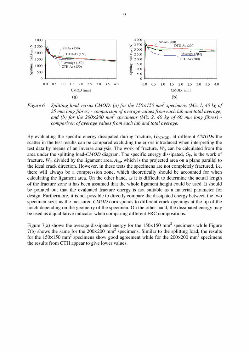
Figure 6. Splitting load versus CMOD: (a) for the 150×150 mm2 specimens (Mix 1, 40 kg of

35 mm long fibres) - comparison of average values from each lab and total average;

and (b) for the 200×200 mm2 specimens (Mix 2, 40 kg of 60 mm long fibres) -

comparison of average values from each lab and total average.

By evaluating the specific energy dissipated during fracture, Gf.CMOD, at different CMODs the scatter in the test results can be compared excluding the errors introduced when interpreting the test data by means of an inverse analysis. The work of fracture, Wf, can be calculated from the area under the splitting load-CMOD diagram. The specific energy dissipated, GF, is the work of fracture, WF, divided by the ligament area, Alig, which is the projected area on a plane parallel to the ideal crack direction. However, in these tests the specimens are not completely fractured, i.e. there will always be a compression zone, which theoretically should be accounted for when calculating the ligament area. On the other hand, as it is difficult to determine the actual length of the fracture zone it has been assumed that the whole ligament height could be used. It should be pointed out that the evaluated fracture energy is not suitable as a material parameter for design. Furthermore, it is not possible to directly compare the dissipated energy between the two specimen sizes as the measured CMOD corresponds to different crack openings at the tip of the notch depending on the geometry of the specimen. On the other hand, the dissipated energy may be used as a qualitative indicator when comparing different FRC compositions. Figure 7(a) shows the average dissipated energy for the 150×150 mm2 specimens while Figure 7(b) shows the same for the 200×200 mm2 specimens. Similar to the splitting load, the results for the 150×150 mm2 specimens show good agreement while for the 200×200 mm2 specimens the results from CTH appear to give lower values.

10

0

200

400

600

800

1 000

0.0 1.0 2.0 3.0 4.0

CMOD [mm]

Dis

sip

ated

en

erg

y, G

f,

[Nm

/m2]

SP-Av (150)

DTU-Av (150)

Average

(150)

CTH-Av (150)

0

250

500

750

1 000

1 250

1 500

0.0 1.0 2.0 3.0 4.0

CMOD [mm]

Dis

sip

ated

en

erg

y, G

f,

[Nm

/m2]

SP-Av (200)

DTU-Av (200)

Average (200)

CTH-Av (200)

(a) (b)

Figure 7. Dissipated energy versus CMOD: (a) for the 150×150 mm2 specimens (Mix 1, 40 kg

of 35 mm long fibres) - comparison of average values from each lab and total

average; and (b) for the 200×200 mm2 specimens (Mix 2, 40 kg of 60 mm long

fibres) - comparison of average values from each lab and total average.

5.2 Intra-lab variation

When testing steel-fibre reinforced concrete it is often found that the scatter is quite large, and the coefficient of variance (Cov) can be as high as 40%. In this study, the coefficient of variance for the splitting load has been calculated, both individually for each lab and for the total test population. In Figure 8(a) the coefficient of variance for the 150×150 mm2 specimens can be seen and Figure 8(b) shows the same for the 200×200 mm2 specimens. The scatter is quite large; for the 150×150 mm2 specimens the average coefficient of variance is around 24% while it is 32% for the 200×200 mm2 specimens. The reason for the scatter being larger for the 200×200 mm2 specimens is believed to be related to the fibre dimensions. The longer fibres lead to a larger scatter since there are fewer fibres present. The coefficient of variance has also been calculated for the dissipated energy, see Figure 9. For the dissipated energy the coefficient of variance is 20% for the 150×150 mm2 specimens respectively 30% for the 200×200 mm2 specimens.

0%

10%

20%

30%

40%

0.0 1.0 2.0 3.0 4.0

CMOD [mm]

Co

effi

cien

t o

f v

aria

nce

[%

]

SP-Av (150)

DTU-Av (150)

Average (150)

CTH-Av (150)

0%

10%

20%

30%

40%

0.0 1.0 2.0 3.0 4.0

CMOD [mm]

Co

effi

cien

t o

f v

aria

nce

[%

]

SP-Av (200)

DTU-Av (200)

Average (200)

CTH-Av (200)

(a) (b)

Figure 8. Coefficient of variance for the splitting load: (a) for the 150×150 mm2 specimens

(Mix 1, 40 kg of 35 mm long fibres) - comparison of values from each lab and total

average; and (b) for the 200×200 mm2 specimens (Mix 2, 40 kg of 60 mm long

fibres) - comparison of values from each lab and total average.

11

0%

10%

20%

30%

40%

0.0 1.0 2.0 3.0 4.0

CMOD [mm]

Co

effi

cien

t o

f v

aria

nce

[%

]

SP-Av (150)

DTU-Av (150)

Average (150)

CTH-Av (150)

0%

10%

20%

30%

40%

0.0 1.0 2.0 3.0 4.0

CMOD [mm]

Co

effi

cien

t o

f v

aria

nce

[%

]

SP-Av (200)

DTU-Av (200)

Average (200)

CTH-Av (200)

(a) (b)

Figure 9. Coefficient of variance for the dissipated energy: (a) for the 150×150 mm2

specimens (Mix 1, 40 kg of 35 mm long fibres) - comparison of values from each lab

and total average; and (b) for the 200×200 mm2 specimens (Mix 2, 40 kg of 60 mm

long fibres) - comparison of values from each lab and total average.

5.3 Inter-lab variation

In this round robin test programme, tests were carried out at three labs. To evaluate the reproducibility of the test method, it is important to determine whether there are significant differences introduced by carrying out the test at different labs. A comprehensive study using statistical methods was carried out to investigate the level of variation obtained for the following parameters:

� the peak-load (Fmax);

� the load at CMOD = 1.0 mm (F1.0);

� the load at CMOD = 2.0 mm (F2.0);

� the load at CMOD = 3.0 mm (F3.0);

� the load at CMOD = 4.0 mm (F4.0); and

� the energy dissipated until a CMOD = 4.0 mm (Gf4.0). In this study, the analysis of variance method (more commonly known as ANOVA) was used. In essence, the ANOVA method is able to indicate whether there are any significant differences in the test results at a particular confidence level. The mathematical basis of this method can be found in books on statistics. After carrying out the analysis, a p-value was computed which is an indication of the difference in the test results. If the p-value is near zero, this casts doubt on the null hypothesis and suggests that at least one sample-mean is significantly different from the other sample-means. The choice of a critical p-value to determine whether the result is judged "statistically significant" is left to the researcher. It is common to declare a result significant if

the p-value is less than 0.05 or 0.01. The level of confidence is represented by the value of α.

Normally, in statistical inferences, a value of α = 0.05 is adopted. This value of α has been used in this study. Generally, the ANOVA has four statistical parameters of interest:

� The Fstatic, which is calculated from the different sets of results and is the ratio of the Mean Squares (MS) for each source, which in turn is the ratio (SS / df) of the Sum of Squares (SS) to the degrees of freedom (df) associated with each source.

� The p-value, which is obtained from statistical tables based on the level of confidence, α, and the calculated degrees of freedom (number of labs and number of specimens).

12

� The Fcritic, which is derived from statistical tables based on the level of confidence, α, and the degrees of freedom associated with the test results.

� The ratio of the Fstatic and the Fcritic. A value greater than unity would indicate that there

is a significant difference between the treatments based on the level of confidence, α.

The results of the ANOVA can be seen in Table 2 and Table 3. The ratio of Fstatic /Fcritic is less than unity for all the considered parameters (for both the 150×150 mm2 and the 200×200 mm2 specimens) and the ANOVA indicate that no significant difference between the treatments other than the internal variation. However, the result for the 200×200 mm2 specimens shows a larger variation, which also can be seen in Figure 6(b) and 7(b) where the results from CTH is lower than the others, and as the scatter for this series is quite large it is possible that more specimens were needed to make a more rigorous conclusions. Hence, the ANOVO indicate no inter-lab variation, possible due to the large test scatter, and the test result can be said to be independent of the testing location and the equipment used (with CMOD-control or without).

Table 2. Compilation of ANOVA results for the 150×150 mm2 specimens (Mix 1, 40 kg of 35

mm long fibres).

ANOVA analysis results for the 150×150 mm2 specimens (Mix 1, 40 kg of 35 mm long fibres)

Considered parameter

Statistical parameters Fmax F1.0 F2.0 F3.0 F4.0 Gf4.0

F static 1.3015 0.4001 0.1610 0.0796 0.2221 0.1654

p-value 0.3053 0.6782 0.8530 0.9239 0.8038 0.8494

F crit 3.8056 3.8056 3.8056 3.8056 3.8056 3.8056

F static /F critic 0.342 0.105 0.042 0.021 0.058 0.043

Table 3. Compilation of ANOVA results for the 200×200 mm2 specimens (Mix 2, 40 kg of 60

mm long fibres).

ANOVA analysis results for the 200×200 mm2 specimens (Mix 2, 40 kg of 60 mm long fibres)

Considered parameter

Statistical parameters Fmax F1.0 F2.0 F3.0 F4.0 Gf4.0

F static 2.2513 1.3092 1.3258 1.1054 0.9818 1.1083

p-value 0.1447 0.2992 0.2950 0.3566 0.3974 0.3557

F crit 3.8056 3.6823 3.6823 3.6823 3.6823 3.6823

F static /F critic 0.592 0.356 0.360 0.300 0.267 0.301

5.4 Comparison of specimens fibre distribution

As the variation in the test results is quite large it was decided to determine and compare the fibre distribution. In all the tested specimens the total number of fibres were counted and the average number of fibres per square centimetre have been compared in Figure 10. Furthermore, the coefficient of variance for the number of fibres per square centimetre can be seen in Figure 11. From the figures it becomes clear that the scatter in the fibre distribution is quite large, for the short fibre (35 mm) the coefficient of variance varies between 6% and 18% while for the long fibre (60 mm) it varies between 28% and 38%.

13

0.0

0.1

0.2

0.3

0.4

0.5

0.6

0.7

0.8

0.9

1.0

CTH 150 DTU 150 SP 150 Average 150

No

. fi

bre

s /

cm2

Max

Average

Min

0.0

0.1

0.2

0.3

0.4

0.5

0.6

0.7

CTH 200 DTU 200 SP 200 Average

200

No

. fi

bre

s /

cm2

Max

Average

Min

(a) (b)

Figure 10. Comparison of the number of fibres per square centimetre: (a) for the 150×150 mm2

specimens (Mix 1, 40 kg of 35 mm long fibres) – max, average, and min; and (b) for

the 200×200 mm2 specimens (Mix 2, 40 kg of 60 mm long fibres) – max, average,

and min.

0%

10%

20%

30%

40%

CTH

150

DTU

150

SP 150

Ave

rage

150

CTH

200

DTU

200

SP 200

Ave

rage

200

Coef

fici

ent of

var

ian

ce [

%]

Figure 11 Coefficient of variance for number of fibres per square centimetre (no. fibres / cm2).

6. INTERPRETATION OF TEST RESULTS

6.1 Results from inverse analysis

As the main benefit from fibre reinforcement is the ability to transfer stress across a crack it is important to characterise the stress-crack opening relationship. The stress-crack opening

14

relationship is also required for advanced (non-linear) analysis of structural behaviour (cracking, crack propagation and fracture). Hence, to show how the test results may be interpreted, inverse analyses were conducted on the averaged load-CMOD curves (the average of all tested

specimens from one mix). The inverse analysis was conducted using a Matlab program, developed at DTU by Østergaard [11]. The programme is based on the cracked hinge model by Olesen [33], see Østergaard & Olesen [34], which uses the fictitious crack concept by Hillerborg

et al. [35], see also Hillerborg [36]. In the cracked hinge model it was assumed that the σ-w relationship could be approximated by a bi-linear function, see Figure 12.

Ec

ε

1

wc w1

b2

a1

a2 w

( )

ctf

wσ

( )( ) ( )

( ) ( )

≤<⋅−

≤≤⋅−=

cct

ct

wwwwabf

wwwafw

122

11 01σ

(b) (a)

1

( )

ctf

εσ

Figure 12. Assumed bi-linear stress-crack opening relationship and definition of the

parameters describing the relationship.

In Table 4 the results of the inverse analyses can be seen and the bi-linear stress-crack opening relationships can be seen in Figure 13. There are some minor differences between the obtained stress-crack opening relationships but the overall agreement is quite good. The largest differences are found in the post-cracking parameters (a1, a2, and b2), which is expected as these are highly influenced by the number, orientation and distribution of fibres. The bi-linear stress-crack opening relationships can be seen in Figure 13. There are some minor differences between the obtained stress-crack opening relationships but the overall agreement is quite good.

Table 4. Results of the inverse analyses on the test results: for the 150×150 mm2 specimens

(Mix 1, 40 kg of 35 mm long fibres) the 200×200 mm2 specimens (Mix 2, 40 kg of 60

mm long fibres).

WST 150 WST 200

fct a1 a2 b2 %error fct a1 a2 b2 %error

[MPa] [mm-1] [mm-1] [-] [MPa] [mm-1] [mm-1] [-]

CTH 2.05 10.01 0.0463 0.399 2.38 CTH 2.18 10.0 0.055 0.48 3.20

DTU 1.98 15.12 0.1187 0.508 2.36 DTU 2.49 22.1 0.041 0.51 2.34

SP 1.90 10.256 0.0748 0.490 2.58 SP 2.46 20.0 0.026 0.54 2.61

Average: 1.98 11.80 0.080 0.47 2.44 Average: 2.37 17.4 0.040 0.51 2.71 Cov: 3.9% 12.5% Cov: 7.2% 5.7%

15

0.0

0.5

1.0

1.5

2.0

2.5

0.0 0.5 1.0 1.5 2.0

Crack opening, w , [mm]

Str

ess,

σw, [M

Pa]

CTH (150)

DTU (150)

SP (150)

Average

0.0

0.5

1.0

1.5

2.0

2.5

3.0

0.0 0.5 1.0 1.5 2.0

Crack opening, w , [mm]

Str

ess,

σw, [M

Pa]

CTH (200)

DTU (200)

SP (200)

Average

(a) (b)

Figure 13. Comparison of stress-crack opening relationships (σ-w) obtained by inverse

analysis: (a) for the 150×150 mm2 specimens (Mix 1, 40 kg of 35 mm long fibres);

and (b) for the 200×200 mm2 specimens (Mix 2, 40 kg of 60 mm long fibres).

6.2 Results from simplified analysis

A residual tensile stress, ftR, can be determined by the simplified approach, see Section 2. The relationships between CMOD and CTOD (eq. 2 & 3) can be used to calculate the corresponding crack opening, w.

For the 150×150 mm2 WST-specimens, the relationship between the CMOD and the CTOD is given by eq. 2. This leads to a crack opening, w=2.20 mm, for a maximum CMOD of 4.0 mm.

For the 200×200 mm2 WST-specimens, the relationship between the CMOD and the CTOD is given by eq. 3. This leads to a crack opening, w=2.12 mm, for a maximum CMOD of 4.0 mm. Figure 14 shows the external forces acting on the specimen and the internal forces, based on the simplified stress distribution. The residual tensile stress, ftR can be calculated by solving the equilibrium equation of forces (eq. 6) and the equilibrium equation of moment with respect to the position of the neutral axis (eq. 6):

16

Fsp

Position of CMOD

CTOD Fsp

x

h*

(a) (b)

ftR

Fc

FtR Fv/2 dy

dx +CMOD

Fv/2

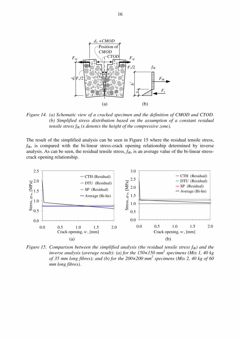
Figure 14. (a) Schematic view of a cracked specimen and the definition of CMOD and CTOD.

(b) Simplified stress distribution based on the assumption of a constant residual

tensile stress ftR (x denotes the height of the compressive zone).

The result of the simplified analysis can be seen in Figure 15 where the residual tensile stress, ftR, is compared with the bi-linear stress-crack opening relationship determined by inverse analysis. As can be seen, the residual tensile stress, ftR, is an average value of the bi-linear stress-crack opening relationship.

0.0

0.5

1.0

1.5

2.0

2.5

0.0 0.5 1.0 1.5 2.0Crack opening, w , [mm]

Str

ess,

σw, [M

Pa]

CTH (Residual)

DTU (Residual)

SP (Residual)

Average (Bi-lin)

0.0

0.5

1.0

1.5

2.0

2.5

3.0

0.0 0.5 1.0 1.5 2.0

Crack opening, w , [mm]

Str

ess,

σw, [M

Pa]

CTH (Residual)

DTU (Residual)

SP (Residual)

Average (Bi-lin)

(a) (b)

Figure 15. Comparison between the simplified analysis (the residual tensile stress ftR) and the

inverse analysis (average result): (a) for the 150×150 mm2 specimens (Mix 1, 40 kg

of 35 mm long fibres); and (b) for the 200×200 mm2 specimens (Mix 2, 40 kg of 60

mm long fibres).

17

7. CONCLUDING REMARKS

To evaluate the reproducibility of the wedge-splitting test method, a round robin study was conducted in which three labs participated (see Löfgren et al. [1]). The participating labs were:

� DTU – the Technical University of Denmark, Department of Civil Engineering;

� CTH – Chalmers University of Technology, Department of Structural Engineering and Mechanics; and

� SP –Swedish National Testing and Research Institute. Two different mixes were investigated; the difference between the mixes was the fibre length (Mix 1 with 40 kg of 35 mm long fibres and Mix 2 with 40 kg of 60 mm long fibres). The test results from each lab were analysed and a study of the variation was performed. From the study of the intra-lab variations, it is evident that the variations of the steel fibre-reinforced concrete properties are significant. The coefficient of variance for the splitting load was found to vary between 20% and 35% for the 150×150 mm2 specimens (Mix 1, 40 kg of 35 mm long fibres) while for the 200×200 mm2 specimens (Mix 2, 40 kg of 60 mm long fibres) it varied between 25% and 40%. The investigation of the inter-lab variation, based on an analysis of variance (ANOVA) indicated no inter-lab variation, possible due to the large scatter in the test results. It is possible that more specimens or labs were required to make a more rigorous conclusions. However, the result of this study indicate that the test results can be said to be independent of the testing location and the equipment used (with or without CMOD-control). The conclusions that can be drawn from this study are that:

� the wedge-splitting test method is a suitable test method for assessment of fracture properties of steel fibre-reinforced concrete;

� the test method is easy to handle and the execution is relatively fast;

� the test results were found to be independent of the testing location and the equipment used;

� the test can be run with CMOD-control or without, in a machine with a constant actuator displacement rate (if the rate is equal to or less than 0.25 mm/min);

� due to variations in fibre distribution, the scatter of the test results is high (but not higher than for the three-point bending test);

� the dimensions of the specimen (height, width, and thickness) should be at least more than three times the fibre length, or preferably four times the maximum fibre length;

� using inverse analysis, the tensile fracture properties may be interpreted from the test results as a bi-linear stress-crack opening relationship.

ACKNOWLEDGMENT

This paper is a product of the NORDTEST, project No. 04032 (1672-04, Part I). The financial support from the NORDTEST organisation is greatly appreciated.

18

REFERENCES

[1] Löfgren, I., Olesen J.F., and Flansbjer, M.: ‘Application of WST-method for fracture testing of fibre-reinforced concrete’. Report 04:13, Department of Structural Engineering and Mechanics, Chalmers University of Technology, Göteborg 2004, pp 52.

[2] Romualdi, J.P. and Mandel, J.A.: ‘Tensile strength of concrete affected by uniformly distributed and closely spaced short lengths of wire reinforcement’. ACI J. Proc. 61(6) 1964, pp. 657-671.

[3] ACI Committee 544: ‘Measurement of properties of fiber reinforced concrete’. ACI Materials

Journal 85(1988), pp. 583-593. [4] ASTM C 1018: ‘Standard Test Method for Flexural Toughness and First-Crack Strength of

Fiber-Reinforced Concrete (Using Beam With Third-Point Loading),’ ASTM, West Conshohocken, Pa., 1997.

[5] ASTM C 1550: ‘Standard Test Method for Flexural Toughness of Fiber-Reinforced Concrete

(Using Centrally-Loaded Round Panel),’ ASTM, West Conshohocken, Pa., 2002. [6] Gopalaratnam, V.S. and Gettu, R.: ‘On the characterization of flexural toughness in fiber

reinforced concretes’. Cem. & Concrete Composites 17(1995), pp. 239-254. [7] Barr B., Gettu R., Al-Oraimi S.K.A., and Bryars L.S.: ‘Toughness measurement – the need to

think again’. Cem. & Concrete Composites 18(1996), pp. 281-297. [8] RILEM TC TDF-162: ‘Test and design methods for steel fibre reinforced concrete. Bending test –

Final Recommendation’, Materials and Structures, 35, Nov 2002, pp. 579-582. [9] RILEM TC TDF-162: ‘Test and design methods for steel fibre reinforced concrete.

Recommendations for uni-axial tension test’, Materials and Structures, 34 Jan-Feb 2001, pp. 3-6. [10] RILEM TC-50 FMC: ‘Determination of the fracture energy of mortar and concrete by means of

three-point bend tests on notched beams’, Materials and Structures, 18(106), 1985, pp. 285. [11] Østergaard, L.: ‘Early-Age Fracture Mechanics and Cracking of Concrete – Experiments and

Modelling’. Ph.D thesis, Department of Civil Engineering, Technical University of Denmark. 2003.

[12] Linsbauer, H.N. and Tschegg, E.K.: ‘Fracture energy determination of concrete with cube shaped specimens’, Zement und Beton, 31, pp 38-40.

[13] Brühwiler, E. and Wittmann, F.H.: ‘The wedge splitting test, a new method of performing stable fracture mechanics test’ Eng. Fracture Mech. 35(1/2/3), 117-125.

[14] de Place Hansen, E.J., Hansen, E.A., Hassanzadeh, M., and Stang, H.: Determination of the Fracture Energy of Concrete: A comparison of the Three-Point Bend Test on Notched Beam and the Wedge-Splitting Test. NORDTEST Project No 1327-97. SP Swedish National Testing and Research Institute, Building Technology, SP Report 1998:09, Borås, Sweden. p. 87.

[15] Trunk, B., Schober, G., and Wittmann, F.H.: ‘Fracture mechanics parameters of autoclaved aerated concrete’, Cem. and Concrete Research, 29(1999), pp. 855-859.

[16] Kim, J.-K. and Kim, Y.-Y.: ‘Fatigue crack growth of high-strength concrete in wedge-splitting test’. Cem. and Concrete Research, 29(1999), pp. 705–712.

[17] Elser, M., Tschegg, E.K., Finger, N., and Stanzl-Tschegg, S.E.: ‘Fracture Behaviour of Polypropylene-Fibre reinforced Concrete: an experimental investigation’, Comp. Science and

Technology, 56(1996), pp. 933-945. [18] Meda, A., Plizzari, G.A., and Slowik, V.: ‘Fracture of fiber reinforced concrete slabs on grade’.

In Fracture Mechanics of Concrete Structures, ed. De Borst et al, 2001. [19] Nemegeer, D., Vanbrabant, J. and Stang, H.: ‘Brite Euram Program on Steel Fibre Concrete

Subtask: Durability: Corrosion Resistance of Cracked Fibre Reinforced Concrete’. In Test and Design Methods for Steel Fibre Reinforced Concrete – Background and Experiences - Proceedings of the RILEM TC 162-TDF Workshop, Ed Schnütgen and Vandevalle, 2003.

[20] Löfgren, I.: ‘The wedge splitting test – a test method for assessment of fracture parameters of

FRC?’. In Fracture Mechanics of Concrete Structures, Li Et al (eds), 2004.

19

[21] Leite, J.P. de B., Slowik, V. and Mihashi, H.: ‘Mesolevel models for simulation of fracture

behaviour of fibre reinforced concrete’. In Fibre-Reinforced Concrete, Proceedings of the Sixth International RILEM Symposium, ed. di Prisco et al. 2004.

[22] RILEM Report 5: Fracture Mechanics Test Methods for Concrete. Edited by S.P. Shah and A. Carpinteri. Chapman and Hall, London, 1991.

[23] Roelfstra, P.E. and Wittmann, F.H.: ‘Numerical method to link strain softening with failure of concrete. In Fracture Toughness and Fracture Energy of Concrete, pp. 163-175. Elsevier, 1986.

[24] Planas, J., Guinea, G.V., and Elices, M.: ‘Size effect and inverse analysis in concrete fracture’, International Journal of Fracture, 95(1999), pp. 367-378.

[25] Bolzon, G., Fedele, R., and Maier, G.: ‘Parameter identification of a cohesive crack model by Kalman filter’, Comput. Methods Appl. Mech. Engrg. 191(2002), pp. 2847-2871.

[26] Que, N.S. and Tin-Loi, F.: ‘Numerical evaluation of cohesive fracture parameters from a wedge splitting test’ Engineering Fracture Mechanics, 69 (2002), pp. 1269-1286.

[27] Kitsutaka, Y.: ‘Fracture parameters by polylinear tension-softening analysis. J. of Eng.

Mechanics, 123(5) pp. 444-450, 1997. [28] Nanakorn, P. and Horii, H.: ‘Back analysis of tension-softening relationship of concrete. J.

Materials, Conc. Struct., Pavements, 32(544), pp. 265-275, 1996. [29] Uchida, Y., Kurihara, N., Rokugo, K., and Koyanagi, W.: ‘Determination of tension softening

diagrams of various kinds of concrete by means of numerical analysis’. In Fracture Mechanics of

Concrete Structures, FRAMCOS-2, ed. F.H. Wittmann, pp. 17-30, 1995. [30] Kooiman, A.G.: ‘Modelling Steel Fibre Reinforced Concrete for Structural Design’. Ph.D. Thesis,

TU Delft 2000.

[31] Sousa, J.L.A.O, Gettu, R., and Barragán, B.E.: ‘Obtaining the σ–w curve from the inverse analysis of the notched beam response’ see Annex D of Barragán, B.E. (2002) ‘Failure and toughness of

steel fiber reinforced concrete under tension and shear’, Ph.D. Thesis, Universitat Politécnica de Catalunya, Barcelona, Spain, 2002.

[32] Löfgren, I., Stang, H. and Olesen, J.F..: ‘Wedge splitting test – a test to determine fracture

properties of FRC’ BEFIB 2004 - Sixth RILEM symposium on fibre reinforced concrete (FRC): Varenna, Italy, 20th-22nd September 2004.

[33] Olesen, J.F.: ‘Fictitious crack propagation in fibre-reinforced concrete beams’. Journal of Eng.

Mech. 127(3): pp. 272-280, 2001. [34] Østergaard, L. and Olesen, JF.: ‘Comparative study of fracture mechanical test methods for

concrete’. In Fracture Mechanics of Concrete Structures, FRAMCOS-5, ed. Li et al, pp. 455-462. [35] Hillerborg, A., Modeer, M., and Petersson, P.E.: ‘Analysis of Crack Formation and Crack Growth

in Concrete by Means of Fracture Mechanics and Finite Elements’. Cem. & Concrete Res. 6, 1976, 773-782.

[36] Hillerborg, A.: ‘Analysis of Fracture by Means of the Fictitious Crack Model, Particularly for Fibre Reinforced Concrete’. The Int. J. Cem. Comp. 1980. 2. 177-184.