The Volatility Risk Premium Embedded in Currency

Options

Buen Sin Low1 and Shaojun Zhang2

JEL Classification: G12, G13 Keywords: volatility risk premium, stochastic volatility, currency option, term structure of risk premium 1Division of Banking and Finance, Nanyang Technological University, Singapore 639798, abslow@ntu.edu.sg, phone: 65-67905753 2Division of Banking and Finance, Nanyang Technological University, Singapore 639798, asjzhang@ntu.edu.sg, phone: 65-67904240

We thank Phillipe Chen, Robin Grieves, William Lee, Paul Malatesta (the editor), Jun Pan, Yonggan Zhao, and the seminar participants at the Nanyang Business School, the 16th Annual Australasian Finance and Banking Conference, and the China International Conference in Finance 2004 for helpful comments and discussions. We especially thank an anonymous referee for his constructive comments and suggestions. Any remaining errors are our own responsibility. We also acknowledge financial support from the Centre for Research in Financial Services at the Nanyang Business School and the Centre for Financial Engineering at the Nanyang Technological University.

1

The Volatility Risk Premium Embedded in Currency Options

Abstract

This study employs a non-parametric approach to investigate the volatility risk

premium in the over-the-counter currency option market. Using a large database of daily

quotes on delta neutral straddle in four major currencies – the British Pound, the Euro, the

Japanese Yen, and the Swiss Franc – we find that volatility risk is priced in all four

currencies across different option maturities and the volatility risk premium is negative.

The volatility risk premium has a term structure where the premium decreases in

maturity. We also find evidence that jump risk may be priced in the currency option

market.

I. Introduction

It has been widely documented in the literature that the price volatility of many

financial assets follows a stochastic process. This leads to the question of whether

volatility risk is priced in financial markets.

Lamoureux and Lastrapes (1993), Coval and Shumway (2001), and Bakshi and

Kapadia (2003), among others, present substantial evidence that volatility risk is priced in

the equity option market and that the risk premium is negative. However, although

foreign currency returns have stochastic volatility (see, e.g., Taylor and Xu (1997)), there

is scant evidence on the market price of volatility risk in currency option markets. In this

paper, we explore the volatility risk premium in currency options.

2

Sarwar (2001) studies the historical prices of the Philadelphia Stock Exchange

(PHLX) currency options on the U.S. Dollar/British Pound from 1993 to 1995, and

reports that volatility risk is not priced for the currency options in the sample. This

finding contrasts with the overwhelming evidence of the existence of volatility risk

premium in the equity options markets. It is also inconsistent with other empirical

findings in the currency option markets. For example, Melino and Turnbull (1990, 1995)

report that stochastic volatility option models with a non-zero price of volatility risk have

less pricing error and better hedging performance for currency options than do constant

volatility option models. Furthermore, Black-Scholes implied volatilities for currency

options have been shown to be biased forecasts of actual volatility (see Jorion (1995),

Covrig and Low (2003), and Neely (2003)). One possible explanation for the bias is the

presence of a volatility risk premium.

Investors are presumably risk-averse and dislike volatile states of the world.

Within the framework of international asset pricing theory, Dumas and Solnik (1995) and

De Santis and Gerard (1998), among others, show that foreign currency securities should

compensate investors for bearing currency risk in addition to the traditional risk due to

the covariance with the market portfolio. As the volatility of currency price is also

uncertain, it introduces additional risk that investors have to bear and should be

compensated for. Assets that lose value when volatility increases are more risky for

investors to hold than those that gain value when volatility increases, such as currency

options. Hence, unlike the case for foreign currency securities in the spot market, where

one may expect a positive risk premium for bearing volatility risk, this may not be the

case for currency options. Coval and Shumway (2001) formalize this intuition in the

3

context of mainstream asset pricing theory and show that options have greater systematic

risk than their underlying securities. They provide evidence that investors are willing to

pay a premium to hold options in their portfolio as a hedge against volatile states of the

world. Thus, this would make the option price higher than its price when volatility risk is

not priced. In other words, the volatility risk premium in currency options would be

negative if it exists.

In this paper, we investigate the volatility risk premium in the over-the-counter

(OTC) currency option market.1 We extend a new methodology proposed by Bakshi and

Kapadia (2003) from equity index options to currency options and apply it to at-the-

money delta neutral straddles traded in the OTC market. An at-the-money delta neutral

straddle is a combination of one European call and one European put with the same

maturity and strike price on the same currency. At-the-money delta neutral straddles are

the most liquid option contracts traded on the OTC market. Because their prices are very

sensitive to volatility, they are widely used to hedge or speculate on changes in volatility.

Therefore, if volatility risk is priced in the currency option market, straddles are the best

instruments through which to observe the risk premium.

Our database includes daily OTC average bid and ask implied volatility quotes for

European at-the-money delta neutral straddles. The database covers the British Pound,

Japanese Yen, and Swiss Franc (against the U.S. Dollar) from June 1996 to December

1 The OTC currency option market is substantially more liquid than the exchange traded currency option

market. The annual turnover of currency options that are traded on organized exchanges was about US$1.3

trillion in 1995 and declined to US$0.36 trillion in 2001 (see Bank for International Settlement (1997,

2003)), whereas the annual turnover on the over-the-counter market was about US$10.25 trillion in 1995

and about US$15 trillion in 2001 (see Bank for International Settlement (1996, 2002)).

4

2002, and the Euro from January 1999 to December 2002. In OTC currency option

market, option prices are quoted in terms of volatility, expressed as a percentage per

annum. For example, an option that is quoted at a 10% bid has the option premium

computed by substituting 10% as the volatility figure into the Garman-Kohlhagen (1983)

model, along with the prevailing current spot exchange rate and domestic and foreign

interest rates.2 One advantage of the data is that the OTC volatility quotes apply to option

contracts of the same standard maturity term, regardless of which day the price is quoted.

We study at-the-money straddles for maturities of 1 month, 3 months, 6 months, and 12

months. Our approach ensures that our implied volatility series are homogeneous with

respect to moneyness and maturity, and that conclusions drawn from analyzing this

database are unlikely to be affected by the mixture of moneyness and maturity.

Our main findings include the following.

• First, we find that volatility risk is priced in four major currencies – the British

Pound, Euro, Japanese Yen, and Swiss Franc – across maturity terms between 1

month and 12 months.3,4

• Second, we provide direct evidence of the sign of the volatility risk premium.

The risk premium is negative for all four major currencies, which suggests that

2 In a study on the term structure of implied volatilities, Campa and Chang (1995) use equivalent OTC

option volatility quotes from December 1989 to August 1992.

3 The results are contrary to the findings of Sarwar (2001). The difference may be because Sarwar (2001)

uses data for exchange-traded options, which are mixed in maturity and moneyness, whereas the quotes of

OTC currency options in our study have constant maturity and apply only for at-the-money options.

4 Evidence of volatility risk premium is also found in four other currencies against U.S. dollar and three

cross currencies. The results are reported in section VI.

5

buyers in the OTC currency option market pay a premium to sellers as

compensation for bearing the volatility risk.

• Third, and more important, we find that the volatility risk premium has a term

structure in which the risk premium decreases in maturity. This study is the first

to provide empirical evidence of the term structure of the volatility risk premium.

Previous studies have documented that short-term volatility has higher variability

than long-term volatility (e.g. Xu and Taylor (1994) and Campa and Chang

(1995)), but none have investigated the implication on volatility risk premiums.

• Fourth, we document that jump risk is also priced in the OTC markets. However,

the observed volatility risk premium is distinct from and not subsumed by the

possible jump risk premium.

All of our findings are robust to various sensitivity analyses on risk-free interest

rates, different sub-periods, and specifications of empirical models.

The paper is organized as follows. Section II details the methodology used in the

study. Section III explains the unique features of OTC currency option markets and the

data. Section IV describes the empirical implementation of the methodology. Section V

presents our main empirical findings and Section VI reports some robustness studies.

Section VII provides a summary and conclusion.

II. Methodology

Bakshi and Kapadia (2003) propose a non-parametric method to investigate

volatility risk premiums in equity index option markets. Under a general stochastic

6

option-pricing framework they prove that if volatility risk is priced in the option market,

then the return of a dynamically delta-hedged call option on a stock index is

mathematically related to the volatility risk premium. Hence, it is theoretically sound to

infer the sign of the volatility risk premium from returns on dynamically delta-hedged

call options. This approach allows the investigation of the volatility risk premium

without the imposition of strong restrictions on the pricing kernel or assuming a

parametric model of the volatility process.

Using this approach, Bakshi and Kapadia (2003) show that volatility risk is priced

in the S&P 500 index option market and that the volatility risk premium is negative. We

extend their methodology to the currency option market.

A. Theory

Assume that the spot price of a currency at time t, xt, follows the process:

(1) tttt

t dzdtmx

dxσ+=

(2) tttt dwdtd δθσ +=

where zt and wt are standard Wiener processes, the random innovations of which have

instantaneous correlation ρ. Parameters mt and σt are the instantaneous drift and

volatility of the currency spot price process; mt can be a function of xt and σt. The

instantaneous volatility σt, follows another diffusion process with mean θt and standard

deviation δt as specified in equation (2), where θt and δt may depend on σt but not on xt.

Let ƒt denote the price of a European straddle on the currency. By Ito’s lemma, ƒt

follows the stochastic process characterized by:

7

(3) dtx

fx

fxf

xtf

df

dxxf

dftt

tttt

t

tt

t

ttt

tt

t

tt

t

tt ⎟⎟

⎠

⎞⎜⎜⎝

⎛∂∂

∂+

∂∂

+∂∂

+∂∂

+∂∂

+∂∂

=σ

σρδσ

δσσσ

2

2

22

2

222

21

21

The price change, dƒt is properly interpreted mathematically as the following

stochastic integral equation:

(4)

∫

∫∫

+

+++

⎟⎟⎠

⎞⎜⎜⎝

⎛∂∂

∂+

∂∂

+∂∂

+∂∂

+

∂∂

+∂∂

+=

τ

τττ

σσρδ

σδσ

σσ

t

tuu

uuuu

u

uu

u

uuu

u

t

t uu

ut

t uu

utt

dux

fxfxfx

uf

dfdxxfff

2

2

22

2

222

21

21

Using standard arbitrage arguments (see Cox, Ingersoll and Ross (1985)), the

straddle price, ƒt, must satisfy the following partial differential equation:

(5) 0)()(21

21 2

2

22

2

222 =−

∂∂

+∂∂

−+∂∂

−+∂∂

∂+

∂∂

+∂∂

tt

t

ttt

t

tt

tt

tttt

t

tt

t

ttt rf

tff

xf

xqrx

fx

fxf

xσ

λθσ

σρδσ

δσ

where r and q denote the domestic and foreign risk free rates. The unspecified term, λt,

represents the market price of the risk associated with dwt, which is commonly referred to

as the volatility risk premium (see, e.g., Heston (1993)).

By rearranging equation (5) and substituting it into the last integral of equation

(4), we obtain:

(6) ( ) ( )∫∫∫+++

+ ⎟⎟⎠

⎞⎜⎜⎝

⎛∂∂

−−∂∂

−−+∂∂

+∂∂

+=τττ

τ σλθσ

σt

tu

uuu

u

uuu

t

t uu

ut

t uu

utt du

fxf

xqrrfdf

dxxf

ff

Substituting equation (2) into (6), we can rewrite equation (6) and the straddle

price can be expressed as:

(7) ( ) ∫ ∫∫∫+ +++

+ ∂∂

+∂∂

+⎟⎟⎠

⎞⎜⎜⎝

⎛∂∂

−−+∂∂

+=τ τττ

τ σδ

σλt

t

t

t uu

uu

u

uu

t

tu

uuu

t

t uu

utt dw

fdu

fdu

xf

xqrrfdxxf

ff

We now consider a dynamically delta-hedged portfolio that consists of a long

straddle position and a spot position in the underlying currency. The spot position is

8

adjusted over the life of the straddle (t to t+τ) to hedge all risks except volatility risk. The

outcome of this dynamically delta-hedged portfolio, hereafter referred to as the delta-

hedged straddle profit (loss), is given by:

(8) ( )∫∫++

++ ⎟⎟⎠

⎞⎜⎜⎝

⎛∂∂

−−−∂∂

−−=Πττ

ττt

tu

uuu

t

t uu

utttt du

xf

xqrrfdxxf

ff,

From equation (7) this can also be stated as:

(9) ∫ ∫+ +

+ ∂∂

+∂∂

=Πτ τ

τ σδ

σλt

t

t

t uu

uu

u

uutt dw

fdu

f ,

The second integral in equation (9) is the Ito stochastic integral. Hence, the

martingale property of the Ito integral implies:

(10) ∫+

+ ⎟⎟⎠

⎞⎜⎜⎝

⎛∂∂

=Πτ

τ σλt

tu

uutt du

fEE )( ,

The implication of equation (10) is that if the volatility risk is not priced (i.e., λu =

0), then the delta-hedged straddle profit (loss) on average should be zero. If the volatility

risk is priced (i.e., λu ≠ 0), then the expected delta-hedged straddle profit (loss) on

average must not be zero. Because the vega of a long straddle, u

ufσ∂

∂ , is positive, the

sign of the volatility risk premium, λu, determines whether the average delta-hedged

straddle profit is positive or negative.

B. Testable Implications

The theory suggests that the return on buying a straddle and dynamically delta-

hedging this position until maturity is related to the volatility risk premium. Although the

9

theory requires the assumption of continuous hedging, in practice, rebalancing takes place

only at discrete times.5 Suppose that we rebalance the delta-hedged portfolio at N equally

spaced times over the life of the straddle between time t and t+τ. That is, the hedging

position is calculated at time tn, n = 0, 1, 2, …. N-1, where t0 = t and tN = t+τ. We

compute the delta-hedged straddle profit at the maturity t+τ by:

(11) ( ) ( ) ( )( )N

--0, ,1

0

1

0, 1

ττττ ∑∑

−

=

−

=+++ ∆−−−∆−−−=∏

+

N

nttt

N

ntttttttt nnnnn

xqrrfxxfxkkxMax

where, tf is the straddle premium at time t, τ+tx is the currency price at the maturity t+τ,

k is the strike price of the straddle, nt∆ is the delta of the long straddle, r and q are the

domestic and foreign interest rates. The first term on the right-hand side of the equation

is the payoff of the long straddle at maturity t+τ, the second term is the cost of buying the

straddle at time t, the third term is the rebalancing cost, and the last term adjusts for the

interest expenses on the second and third terms. The delta-hedged straddle profit (loss)

allows us to test the following two hypotheses:

• Hypothesis 1: If, on average, Πt, t+τ is non-zero, then volatility risk is priced in

the currency option market.

• Hypothesis 2: If, on average, Πt, t+τ is negative (positive), then the volatility risk

premium embedded in the currency option is negative (positive).

5 Bakshi and Kapadia (2003) show that the bias in the delta-hedged straddle outcome caused by discrete

hedging is small relative to the effect of a volatility risk premium. Melino and Turnbull (1995) provide

simulation evidence to show that the discrete delta hedging error with daily re-balancing is very small. For

example, their average hedging errors, as a percentage of contract size, for a 1-year at-the-money currency

option are only 0.06% and 0.31% if volatility is assumed to be constant or stochastic, respectively.

10

III. Description of the OTC Currency Option Market and Data

The OTC currency option market has some special features and conventions.

First, the option prices on the OTC market are quoted in terms of deltas and implied

volatilities, instead of strikes and money prices as in the organized option exchanges. At

the time of settlement of a given deal, the implied volatility quotes are translated to

money prices with the use of the Garman-Kohlhagen formula, which is the equivalent of

the Black-Scholes formula for currency options. This arrangement is convenient for

option dealers, in that they do not have to change their quotes every time the spot

exchange rate moves. However, as pointed out by Campa and Chang (1998), it is

important to note that this does not mean that option dealers necessarily believe that the

Black-Scholes assumptions are valid. They use the formula only as a one-to-one non-

linear mapping between the volatility-delta space (where the quotes are made) and the

strike-premium space (in which the final specification of the deal is expressed for the

settlement). Second, competing volatility quotes of option contracts are available on the

market everyday, but only for standard maturity periods, such as 1-week, 1-, 3-, 6-month,

and so on. For example, a 3-month option quote on Monday will become an odd period

(3 months less 1 day) option quote on Tuesday, and competing quotes for this odd period

option are not available on Tuesday. Third, most transactions on the market involve

option combinations. The popular combinations are straddles, risk reversals, and

strangles. Among these, the most liquid combination is the standard delta-neutral

straddle contract, which is a combination of a call and a put option with the same strike.

11

The strike price is set, together with the quoted implied volatility price, so that the delta

of the straddle computed on the basis of the Garman-Kohlhagen formula is zero.

As the standard straddle by design is delta-neutral on the deal date, its price is not

sensitive to the market price of the underlying foreign currency. However, it is very

sensitive to changes in volatility. Because of its sensitivity to volatility risk, delta-neutral

straddles are widely used by participants in the OTC market to hedge and trade volatility

risk. If the volatility risk is priced in the OTC market, then delta-neutral straddles are the

best instruments through which to observe the risk premium. For this reason, Coval and

Shumway (2001) uses delta-neutral straddles in their empirical study of expected returns

on equity index options and find that volatility risk premium is priced in the equity index

option market.

Our main option dataset consists of daily average bid and ask implied volatility

quotes for the 1-, 3-, 6-, and 12-month delta-neutral straddles on four major currencies –

the British Pound, the Euro, the Japanese Yen, and the Swiss Franc6 – at their U.S. Dollar

prices. Our sample spans a period of approximately 7.5 years, from June 3, 1996 to

December 31, 2003. The 2003 data are used for calculating the delta-hedged straddle

profit on the straddle bought in 2002. The data are obtained from Bloomberg, who

collected them at 6 p.m. London time from large banks participating in the OTC currency

option market. Other data collected are synchronized daily average bid and ask spot U.S.

Dollar prices of each currency from Bloomberg. Because the British Pound, Euro, 6 We chose to study currency options on these four currencies because they are the most liquid among all

currencies. According to the Bank for International Settlement (2002), they accounted for approximately

67% of the total size of the OTC currency options traded in April 2001. As a robustness test we also study

seven other less liquid currency options and the results are reported in section VI.

12

Japanese Yen, Swiss Franc, and U.S. Dollar Treasury bill yields that exactly match each

option period are not available, the repurchase agreement interest rates (i.e., repo) for

each currency, which match the option maturity period, are used.7

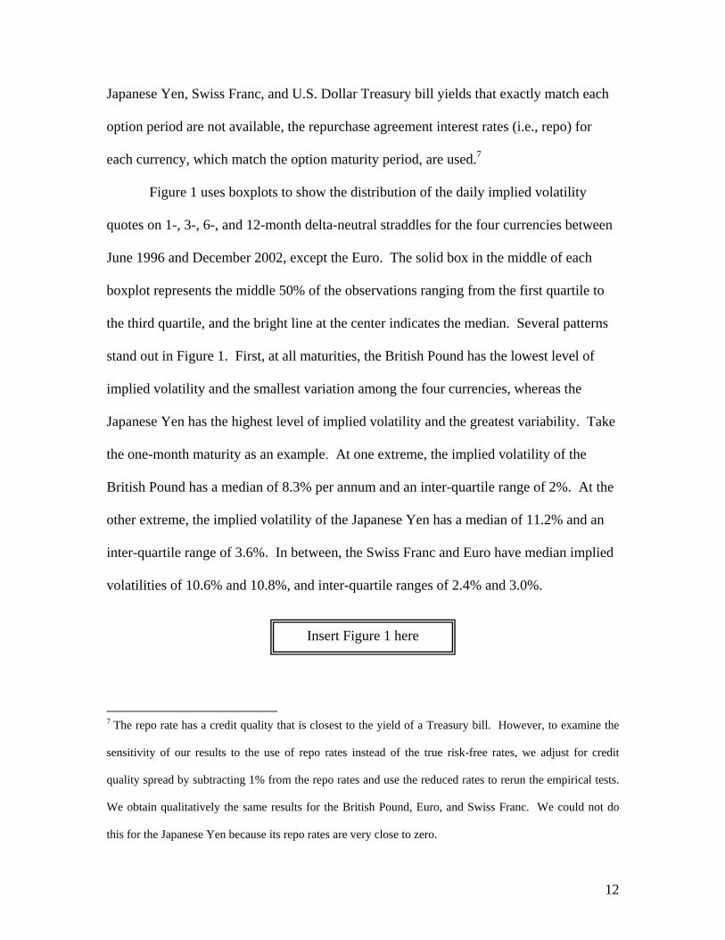
Figure 1 uses boxplots to show the distribution of the daily implied volatility

quotes on 1-, 3-, 6-, and 12-month delta-neutral straddles for the four currencies between

June 1996 and December 2002, except the Euro. The solid box in the middle of each

boxplot represents the middle 50% of the observations ranging from the first quartile to

the third quartile, and the bright line at the center indicates the median. Several patterns

stand out in Figure 1. First, at all maturities, the British Pound has the lowest level of

implied volatility and the smallest variation among the four currencies, whereas the

Japanese Yen has the highest level of implied volatility and the greatest variability. Take

the one-month maturity as an example. At one extreme, the implied volatility of the

British Pound has a median of 8.3% per annum and an inter-quartile range of 2%. At the

other extreme, the implied volatility of the Japanese Yen has a median of 11.2% and an

inter-quartile range of 3.6%. In between, the Swiss Franc and Euro have median implied

volatilities of 10.6% and 10.8%, and inter-quartile ranges of 2.4% and 3.0%.

7 The repo rate has a credit quality that is closest to the yield of a Treasury bill. However, to examine the

sensitivity of our results to the use of repo rates instead of the true risk-free rates, we adjust for credit

quality spread by subtracting 1% from the repo rates and use the reduced rates to rerun the empirical tests.

We obtain qualitatively the same results for the British Pound, Euro, and Swiss Franc. We could not do

this for the Japanese Yen because its repo rates are very close to zero.

Insert Figure 1 here

13

Second, there is a term structure in the variability of the volatility quotes for all

four currencies. Specifically, the variability is a decreasing function of the time-to-

maturity as short-dated options have much higher variability than long-dated options.

Campa and Chang (1995) observe a similar term structure in their sample of OTC

volatility quotes for four major currencies in a different time period. Xu and Taylor

(1994) study the term structure of implied volatility embedded in PHLX traded options

on four currencies and report that long-term implied volatility has less variability than

short-term implied volatility. The term structure in variability of implied volatility is

consistent with a mean-reverting stochastic volatility process (see Stein (1989) and

Heynen, Kemna, and Vorst (1994)). More importantly, it has an implication for the

volatility risk premium. Because the variability of short-term volatility is much higher

than that of long-term volatility, if option buyers were to pay a volatility risk premium,

then they would pay more in short-term options. This means that the volatility risk

premium should have a term structure in which the risk premium is a decreasing function

of maturity. We report empirical evidence in relation to this hypothesis in Section V.

Third, the boxplots show the skewness of the implied volatility distribution. In

each boxplot, the lower bracket connected by whiskers to the bottom of the middle box

indicates the larger value of the minimum or the first quartile less 1.5 times the inter-

quartile range, while the upper bracket connected by whiskers to the top of the middle

box indicates the lower value of the maximum or the third quartile plus 1.5 times the

inter-quartile range. For a right-skewed distribution, the upper bracket is further away

from the box than the lower bracket; the pattern reverses for a left-skewed distribution.

The lines beyond the lower or upper bracket represent outliers. The four currencies differ

14

in skewness of implied volatility. While the British Pound and the Swiss Franc have

close-to symmetric distributions, the distributions of the Euro and the Japanese Yen are

clearly right skewed and the Yen has far more outliers (i.e., a much fatter tail) than the

other three currencies. A close examination shows that a majority of the outliers in the

Yen occurred during the Asian currency crisis in 1997 and 1998. Figure 2 shows the time

series plot of the implied volatility for the 3-month at-the-money straddle for the British

Pound, the Japanese Yen, and the Swiss Franc between June 1996 and December 2002.

The two vertical dash lines indicate the start and the end of the Asian currency crisis.

The crisis dramatically changed the price process of the Japanese Yen during that period,

but had little effect on the British Pound and Swiss Franc. This suggests that we should

conduct a robustness analysis for the post-crisis sub-period.

IV. Empirical Implementation

Following the theory discussed in Section II, we now consider portfolios of

buying delta-neutral straddles and dynamically delta-hedging our positions until maturity.

We rebalance the delta-hedged portfolio daily and measure the delta-hedged straddle

profit (loss) from the contract date t to the maturity date t+τ, Πt, t+τ, by the formula

( ) ( ) ( )( )N

--0, ,1

0

1

0, 1

ττττ ∑∑

−

=

−

=+++ ∆−−−∆−−−=∏

+

N

ntttttt

N

ntttttttt nnnnn

xqrfrxxfxkkxMax

Insert Figure 2 here

15

where k denotes the strike price of the straddle, and nt

∆ is the delta of the straddle based

on the Garman-Kohlhagen model,

(12) ( ) ( )[ ]12 1 −=∆ +− dNe nt

n

tqt

τ

( )

τσ

τσ

+

+⎟⎠⎞

⎜⎝⎛ +−+

=nt

ntttt

t

tqrk

x

dn

n

n 2

121ln

where and N(d1) is the cumulative standard

normal distribution evaluated at d1. The Garman-Kohlhagen model, as an extension of

the Black-Scholes model to currency options, is a constant volatility model. Hence, the

delta computed from the Garman-Kohlhagen model may differ from the delta computed

from a stochastic volatility model. We mitigate this problem by adopting a modified

Garman-Kohlhagen model, in which the volatility that is employed to compute the delta

for daily rebalancing is updated based on the daily average bid and ask implied volatility

quotes. Chesney and Scott (1989) conclude that actual prices on foreign currency options

conform more closely to this modified Garman-Kohlhagen model than to a stochastic

volatility model or to a constant volatility Garman-Kohlhagen model. Bakshi and

Kapadia (2003) also provide a simulation exercise to show that using the Black-Scholes

delta hedge ratio, instead of the stochastic volatility counterpart, has only a negligible

effect on delta-hedged results. We report a robustness study in section VI that examines

the impact of potential mis-measurement of the hedge ratio

More specifically, we take the following two steps to maintain the delta-hedged

portfolio until the maturity. First, we need to compute the money price for the straddle.

This is achieved by a one-to-one mapping between the volatility-delta space and the

strike-premium space using the Garman-Kohlhagen model. For an observed implied

volatility quote on day t, the strike price of the delta-neutral straddle is determined by the

16

formula τσ )5.0( 2ttt qr

texk +−= , where tx denotes the synchronized spot foreign currency

price on day t, tr and tq are the domestic and foreign interest rates per annum, τ is the

time-to-maturity expressed in years, and σt is the average bid and ask implied volatility

quote.8 This strike price formula is used in the OTC market by convention. The straddle

premium is then computed using the Garman-Kohlhagen model, together with the

computed strike price, the synchronized spot foreign currency price, and interest rates.

Second, we form and maintain the delta-hedged portfolio until the maturity.

Suppose that, on day t, we bought a straddle contract at the premium computed as above.

As the straddle is in itself delta neutral, the delta-hedged portfolio on day t is composed

of only the straddle. However, on the following day t+1, the straddle becomes an odd-

period contract and may no longer be delta neutral. Hence, to maintain a delta-hedged

portfolio, we need to sell the delta amount of the foreign currency against the U.S. Dollar

at the day t+1spot price. We therefore re-compute the delta using Equation (12) with the

spot price, interest rates, and the estimated volatility of an odd-period straddle contract at

day t+1.9 We estimate the volatility of an odd-period straddle contract using the linear

total variance method (see Wilmott (1998)) to interpolate the volatility of standard

maturities:

(13) ( )2

1

21

23

13

1221

21312

1⎥⎦

⎤⎢⎣

⎡−⎟⎟

⎠

⎞⎜⎜⎝

⎛−−

+= TTTT TTTTTTT

Tσσσσ

8 Equation (12) shows that the delta of a straddle is zero only when d1 = 0. The strike price is computed in

such a way that d1 = 0.

9 We cannot use the quoted volatility on day t+1 because volatility quotes are valid only for straddles of

standard maturities such as 1 month or 3 months. Volatility has to be estimated for odd-period straddles.

17

where T1 < T2 < T3, 1Tσ and 3Tσ denote the average bid and ask implied volatility quotes

for the standard maturities T1 and T3 available in the market, and 2Tσ is the volatility for

the non-standard maturity T2 that we need to estimate by interpolation. We also update

the interest rates on a daily basis in rebalancing the delta-hedged portfolio. The foreign

currency sold (bought) is borrowed (invested), and the corresponding long (short) U.S

Dollar cash (net of the straddle premium incurred at time t) is invested (borrowed) at their

respectively interest rates. We continue to rebalance the delta-hedged portfolio on a daily

basis until the straddle maturity date. The net U.S. Dollar payoff is the delta-hedged

straddle profit (loss).

V. Empirical Results

A. Negative Volatility Risk Premium

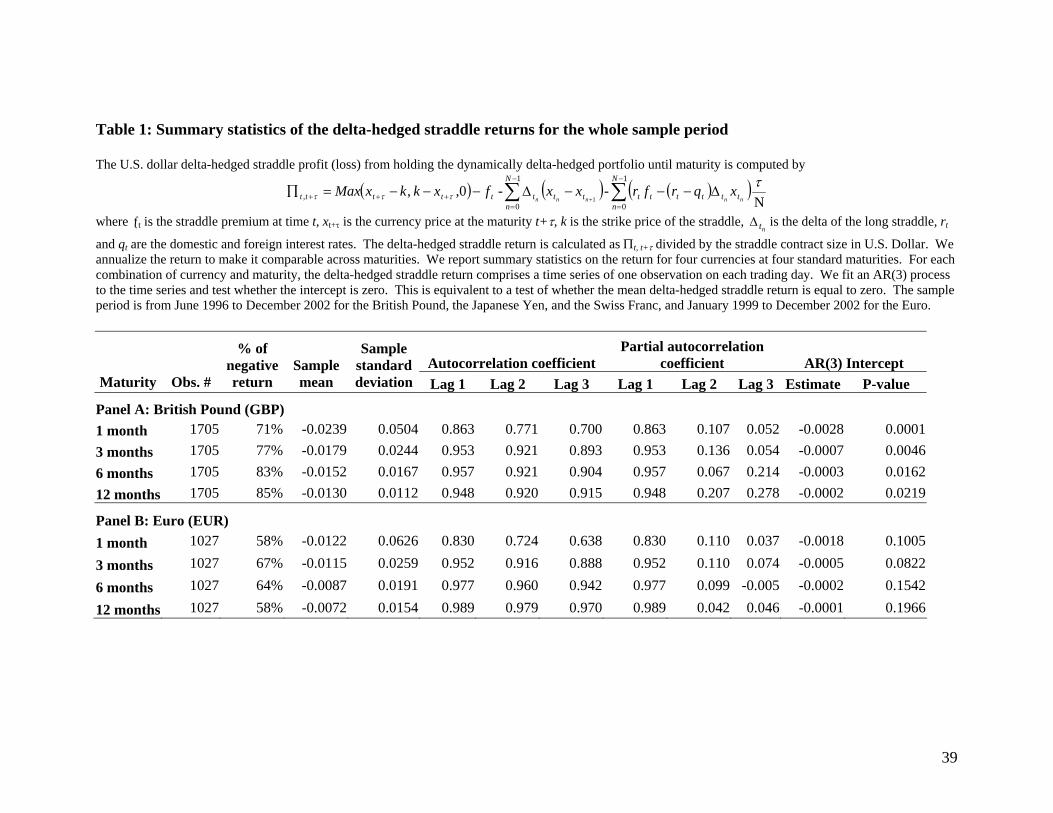
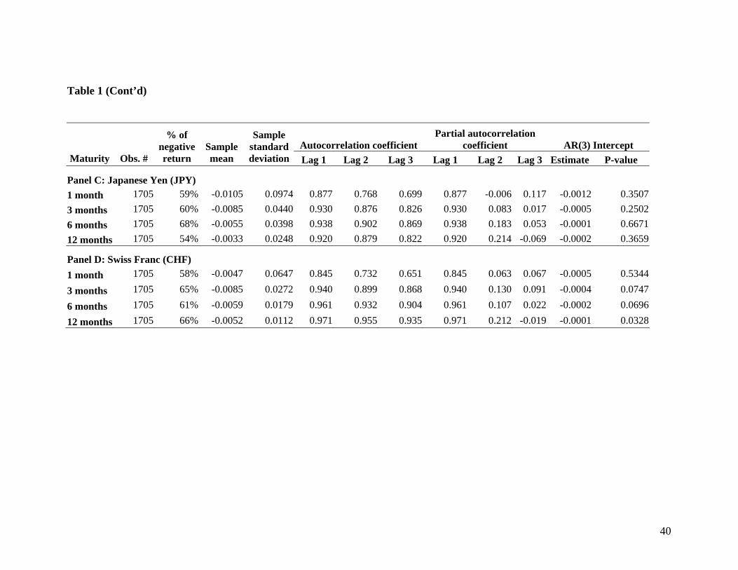
In this section, we document our empirical findings. Table 1 reports the statistical

properties of the delta-hedged straddle returns on four currencies at four maturities. The

delta-hedged straddle returns are calculated as the U.S. Dollar delta-hedged straddle

profit (loss) from holding the dynamically delta-hedged portfolio until maturity, divided

by the straddle contract size in U.S. Dollars. We annualize the returns to make them

comparable across maturities. For each combination of currency and maturity, delta-

hedged straddle returns comprise a time series of daily observations. This arises because,

for each standard maturity, we buy an at-the-money delta neutral straddle each trading

day and maintain a delta-hedged portfolio of the straddle and underlying currencies until

the straddle matures. The first column of Table 1 lists the number of observations in each

18

time series. The Euro has fewer observations than the other three currencies because it

only came into existence in January 1999. In the second column, we report the

percentage of daily straddle observations that have negative returns when we buy a

straddle and maintain the delta-hedged portfolio until maturity. The percentage is much

bigger than 50% in all cases, and is 85% for the British Pound at the 12-month maturity.

This indicates that for most of the time, OTC straddle sellers earn positive profits by

selling straddles and hedging their exposures. According to the theory in Section II, this

suggests that such profits are a compensation for bearing the risk of volatility changes.

The high percentage of negative delta-hedged straddle returns indicates that our results

are not biased by outliers.

We now investigate whether delta-hedged straddle returns are statistically

significant. The unconditional means and standard deviations of delta-hedged straddle

returns are listed in the third and fourth columns of Table 1. The mean return is negative

for all cases10. The high standard deviations of the returns make the means appear

insignificantly different from zero. However, it is misleading to use the unconditional

standard deviation to test the mean, because serial correlation in the time series of delta-

10 We have run the empirical tests using the average bid and ask straddle prices to reduce the impact of bid

ask spread if there is any. We have also run the empirical tests using both the bid prices and the ask prices.

The results are qualitatively similar to those using straddle average bid and ask prices.

Insert Table 1 here

19

hedged straddle returns can cause the standard deviation to be a biased measure of actual

random error. The next three columns of Table 1 show that the first three autocorrelation

coefficients are quite large and decay slowly. This indicates that the time series may

follow an autoregressive process. We calculate the partial autocorrelation coefficients in

Table 1. The first order partial autocorrelation coefficient is large in all cases, while the

second and third order autocorrelation coefficients become much smaller. The pattern

exhibited in both autocorrelation coefficients and partial autocorrelation coefficients

suggests fitting an autoregressive process of order 3 (i.e., AR(3)) to the time series of the

delta-hedged straddle returns.11 An AR(3) process can be represented by the following

model: 332211 ttttt yyyy εβββα ++++= −−− , where tε is a white noise process. Its

unconditional mean is given by the formula

3211)(

βββα

−−−=tyE

which implies that the null hypothesis of a zero unconditional mean is equivalent to the

null hypothesis that the intercept of the AR(3) process is equal to zero.

We estimate parameters of the AR(3) process and report the estimated intercept

and its p-value for the t-statistic in the last two columns of Table 1. The intercept is

significantly negative in most cases for the British Pound, the Euro, and the Swiss Franc,

whereas it is negative, although insignificant, for the Japanese Yen. We suspect that the

non-significance of the Japanese Yen is due to the Asian currency crisis. Hence, in

11 In an unreported analysis, we also fit AR(1) and AR(5) processes to the data and observe the same

patterns.

20

Section VI we report a robustness analysis for the post-crisis sub-period from July 1999

to December 2002.

Relying on the general equilibrium model of Cox, Ingersoll and Ross (1985), Heston

(1993) and Bates (2000), among others, suggest that the volatility risk premium is

positively related to the level of volatility. To control for the level of volatility, we

consider the following model for the delta-hedged straddle returns:

(14) 332211 tttttt yyyy εβββγσα +++++= −−−

where yt is the delta-hedged straddle return, and σt is the implied volatility. We include

three lagged variables 1−ty , 2−ty , and 3−ty , to control for serial correlation.

Table 2 reports the results of estimating the above model for four currencies at

four maturities. The coefficient of implied volatility, γ, is negative for all currencies at all

maturities. To test its significance, we use the t-test statistic based on Newey-West

(1987) heteroskedasticity and autocorrelation consistent standard errors. The test shows

that γ is significantly negative in all cases. This again provides evidence that market

volatility risk is priced in the OTC currency option markets.

B. Effect of Overlapping Period

We obtain our daily delta-hedged straddle returns by purchasing a straddle and

maintaining a delta-neutral portfolio using the spot currency market until the straddle

matures. In calculating the delta-hedged return of the 1-month straddle bought on a given

Insert Table 2 here

21

trading day, say day 0, we use the information of day 1, day 2, up to day 22, assuming

that there are 22 trading days before the straddle maturity date. Then, for the delta-

hedged return of the 1-month straddle bought on day 1, we use information of day 2, day

3, up to day 23. Consequently, the delta-hedged returns of day 0 and day 1 straddles use

information from an overlapping period between day 2 and day 22. There is a concern

whether our earlier evidence of a negative risk premium is driven by the common

information in the overlapping periods. To address this issue, we adopt the following

two approaches:

In the first approach, we construct a time series of non-overlapping delta-hedged

straddle return for each currency. Specifically, for each currency, we construct a monthly

series of delta-hedged returns on the 1-month straddles bought at the first trading day of

every month in our sample period.12 As the delta-hedged returns of the beginning-of-

month straddle only depend on the information of the trading days in the same month,

they are non-overlapping. Panel A of Table 3 reports the summary statistics for the non-

overlapping returns for the four major currencies. Consistent with the earlier results in

Table 1, the mean delta-hedged returns are negative across all four currencies.

To ascertain whether the volatility risk premium remains negative for non-

overlapping series, we run the following regression

(15) 1 tttt yy εγσα +++= −

where yt is the delta-hedged straddle return, and σt is the volatility quote. If the

volatility risk is priced and has a negative premium, then we expect γ to be significant

12 We consider only the 1-month maturity because too few non-overlapping delta-hedged returns are

available for longer maturities for any meaningful analysis.

22

and negative. Panel B of Table 3 reports the results. The evidence supports the

conclusion that volatility risk is priced and has a negative risk premium.

In the second approach, we remove the effect of the common information from

the overlapping period by calculating the difference between two consecutive delta-

hedged straddle returns. In other words, we study the difference series, 1−−=∆ ttt yyy ,

where ty is the delta-hedged return on a delta-neutral straddle bought on date t . Since

the straddle prices differ between the two days and the straddle return is proportional to

the volatility risk premium as equation (10) shows, we expect to observe the risk

premium in the regression of the first difference of delta-hedged straddle return on the

first difference of implied volatility. Therefore, we run the following regression for ∆yt:

(16) 332211 ttDtDtDtDDt yyyy εβββσγα +++++= −−− ∆∆∆∆∆

where ty is the delta-hedged return on a delta-neutral straddle bought on date t , ty∆ is

the difference between ty and 1−ty , tσ is the volatility quoted for a delta-neutral straddle

on date t , and tσ∆ is the difference between tσ and 1−tσ . We include three lags of the

dependent variable to control for potential serial autocorrelation in ty∆ . If the volatility

risk premium exists and is negative, we expect the coefficient of tσ∆ to be significant

and negative.

Table 4 reports the estimation results of equation (16). The coefficient of implied

volatility, Dγ , is negative for all currencies at all maturities. The t-test statistic based on

Insert Table 3 here

23

Newey-West (1987) heteroskedasticity and autocorrelation consistent standard errors

shows that γ is significantly different from zero in all cases. This evidence provides

further support that market volatility risk is priced in currency option markets.

C. Term Structure of Volatility Risk Premium

The empirical results so far have shown that volatility risk is priced in the OTC

currency option markets and it has a negative risk premium. However, they reveal

further information about the term structure of the volatility risk premiums. Previous

studies such as those of Campa and Chang (1995) and Xu and Taylor (1994) report that

volatility itself is more volatile at short-term maturities than at long-term maturities. The

pattern is also evident in Figure 1. This means that short-term options carry higher

volatility risks than long-term ones. Hence, it is reasonable to expect that currency option

buyers pay a higher volatility risk premium for shorter maturity options as a

compensation to option sellers for bearing higher volatility risks. Consistent with this

expectation, Table 1 shows that the average delta-hedged straddle return decreases when

the option maturity is extended. Table 2 and table 4 show that the coefficients of implied

volatility, γ and γD, also exhibit a term structure. Because γ is the coefficient of volatility,

it can be regarded as the average delta-hedged straddle return per unit of volatility. We

call this the unit delta-hedged straddle return. We observe that the magnitude of the unit

delta-hedged straddle return decreases with maturity. Because the vega of at-the-money

Insert Table 4 here

24

options is an increasing function of maturity (see, e.g., Hull (2003)), the downward

sloping term structure in the magnitude of the unit delta-hedged straddle return is unlikely

to be due to vega. This evidence, combined with equation (10), suggests that the

magnitude of the volatility risk premium decreases with option maturity, which is

consistent with the fact that short-term volatility is more volatile than long-term volatility.

To test whether the observed difference between the short-term volatility risk

premium and the long-term volatility risk premium is statistically significant, we estimate

the following model on the combined time series across the four maturities:

(17)

tttt

tttt

t

yyyIIII

IIIIy

εβββσγσγσγσγ

αααα

+∆+∆+∆+∗∆+∗∆+∗∆+∗∆

++++=∆

−−− 332211

12,12126,663,331,11

1212663311

where ty is the delta-hedged return on a delta-neutral straddle bought on date t , ty∆ is

the difference between ty and 1−ty , ti,σ is the quoted volatility for the i -month maturity

on date t , tσ∆ is the difference between tσ and 1−tσ , and iI is the indicator variable of

an observation for the i -month maturity with i being 1, 3, 6 or 12. We use iα to allow

different intercepts at different maturities.

The estimation results are reported in Table 5. The volatility risk premium

presents a term structure for all four currencies. We use the Wald statistic to test two null

hypotheses: one is 121 γγ = and the other 12631 γγγγ +=+ . The test rejects the two null

hypotheses in all cases, which suggests that the difference between short-term and long-

term volatility risk premiums is significant. This finding implies that the option buyer is

25

paying a significantly higher volatility risk premium to the option seller for the shorter

maturity option.

VI. Robustness Analysis A. Other Currency Pairs

To investigate whether our results are a special feature of the four currencies

selected or whether they apply more broadly, we examine seven other currency pairs.

They are selected based on the liquidity of the option contract and the availability of data.

Four of the seven currency pairs are the Australian Dollar, Canadian Dollar, Norwegian

Kroner, and New Zealand Dollar against the U.S. Dollar. The other three are cross

currency pairs and they are the Japanese Yen against British Pound, the Japanese Yen

against Euro, and the Euro against Swiss Franc.

As these seven currency pairs are less liquid than the four selected currency pairs

in the OTC option market, Bloomberg does not have complete daily straddle quotes from

June 1996 to December 2003. We include only observations before December 2003 that

have complete data necessary for our empirical analysis. The sample size for each

currency pairs is reported in Table 6.

We replicate the analysis based on Equations (16) and (17) for these seven

currency pairs. Table 6 shows that the coefficient of implied volatility in equation (16) is

Insert Table 5 here

26

negative and significant. This is consistent with the earlier observations for the four

major currency pairs, and demonstrates that volatility risk is also priced in the OTC

market for these seven currency pairs.

Table 7 reports the estimation results of Equation (17) and provides evidence on

the term structure in volatility risk premium. Consistent with the evidence in the British

Pound, Euro, Japanese Yen and Swiss Franc against U.S. dollar, the volatility risk

premium presents a term structure for all seven currencies. The magnitude of the short-

term risk premium is greater than its long-term counterpart. The two Wald tests show

that the difference is significant.

B. Post-Asian Currency Crisis Period

In this subsection, we report a sub-period analysis that serves two purposes: to

examine the temporal stability of the volatility risk premium, and to rule out the

possibility that our main findings may be affected by the Asian currency crisis. We

replicate the analysis for the post-crisis period between July 1, 1999 and December 31,

2002. Table 8 reports the results for the post-crisis period. We observe the same

properties of the delta-hedged straddle returns as in Table 1. The main difference

between Table 8 and Table 1 lies in the results for the Japanese Yen. During the post-

Insert Table 7 here

Insert Table 6 here

27

crisis period, the mean return is significantly negative for the Yen, whereas it is not for

the whole period. A possible explanation is that the Asian currency crisis affected the

Yen more than the other three currencies, which causes the distribution of the Yen’s

implied volatility to differ a lot during and after the crisis. Figure 3 shows that the

distribution is less right-skewed for the Yen in the post-crisis period than for the whole

period.

Table 9 reports the estimation results of Equation (16) for the post-Asian currency

crisis period. It shows the same evidence as in Table 4 that the volatility risk premium is

significantly negative for the four currencies and the four maturities under our study.

C. Impact of Jump Risk

Recent studies suggest that option prices account for not only the stochastic

volatility in the return distribution of underlying assets, but also the potentially large tail

events.13 Theoretical option pricing models have been developed to incorporate both

stochastic volatility and potential jumps in the underlying return process (see Pan (2002)

13 See, for example, Bakshi, Cao, and Chen (1997), Bates (2000), Duffie, Pan, and Singleton (2000),

Eraker, Johannes, and Polson (2000), and Pan (2002) for theoretical analysis and empirical evidence.

Insert Table 8 here

Insert Figure 3 here

Insert Table 9 here

28

and the references therein). Hence, it is possible that part of the risk premium observed

in our empirical results is due to jump risk rather than volatility risk. In this section, we

conduct further analysis to show that the volatility risk premium is distinct from the jump

risk premium and is indeed a portion of the option price.

To isolate the potential effect of jump risk, we need to examine the delta-hedged

straddle returns for a sample where jump fears are much less pronounced. We do so by

identifying the days where jump fears are high and exclude them from the sample. We

argue that large moves in currency prices cause market participants to revise upwards

their expectation of future large moves. This is consistent with the fact that GARCH type

models are adequate for the return process of financial assets (see, e.g., Bollerslev, Chou,

and Kroner (1992)). Jackwerth and Rubinstein (1996) report that after the October 1987

market crash, the risk-neutral probability of a large decline in the equity market index is

much higher than before the crash. Hence, jump fears are likely to be high after large

moves in currency prices. We identify the dates when currency prices experienced large

moves so that the daily percentage change is two standard deviations away from the mean

daily percentage change in our sample period. The first column of Table 10 reports the

number of days that experienced a large move in currency prices. We do not differentiate

between negative and positive jumps because the straddle price is equally sensitive to

moves in both directions. Take the British Pound as an example. Between June 3, 1996

and December 31, 2002, 103 days (about 6%) experienced large moves in the U.S. dollar

price of the British Pound in either a positive or a negative direction. The Euro has a

lesser number of large move days because of its shorter trading history. We found that

the average delta-hedged straddle returns remain significantly negative for all currencies

29

after we exclude from the sample the delta-hedged straddle returns of those days when

large moves occurred and also the days immediately after.

Furthermore, we compare the mean and the median of delta-hedged straddle

returns in the day before large moves with those in the day after. The results are reported

in Table 10. The t- and Wilcoxon tests show that both the mean and median of the delta-

hedged straddle returns are significantly negative in most cases before and after large

moves.14 However, the most salient feature is that, for all currencies and across all

maturities, the delta-hedged straddle return is significantly more negative in the day after

than the day before. To control for the effect of variability between the days on the

before-versus-after comparison, we calculate the return difference between before and

after for each large move day and compute the mean and median of the differences. The

results are reported in the last two columns of Table 10. The within-day difference

clearly shows that the magnitudes of delta-hedged straddle returns are significantly larger

in the day after than the day before jumps. It is likely that after price jumps, the market

perceives a high risk of jumps and thus option buyers pay an additional premium to

option sellers for bearing jump risk on top of the volatility risk. This finding provides

evidence that jump risk is priced in the currency option market. However, that the delta-

hedged straddle returns are negative at most times, even on the days before jumps when

14 A close look at the dates of large moves show that the dates are set widely apart, which makes it safe to

assume independence in the sample of delta-hedged straddle returns and use t- and Wilcoxon tests. This

also suggests that although large moves cause market participants to raise their expectations of future

jumps, few large moves of the same magnitude happened consecutively because of the mean-reverting

nature of the return process.

30

jump risk is much less pronounced, indicates that the volatility risk premium is distinct

from and not subsumed by the jump risk premium.

D. Effect of Mis-measurement in the Delta Hedge Ratio

Extant theory (e.g. Hull and White (1987, 1988), Heston (1993) and others)

suggests that using a delta hedge ratio computed on the basis of a constant volatility

model such as the Garman-Kohlhagen model may cause bias in hedging performance

when the volatility process is actually stochastic. The bias depends on the correlation

between the volatility process and the underlying asset return process. To mitigate the

potential bias in the delta hedge ratio, we use the modified Garman-Kohlhagen model in

computing the hedge ratio, that is, the volatility is updated daily. Since this modified

Garman-Kohlhagen model may not have fully corrected the mis-specification, we

estimate the following model for the delta-hedged straddle returns:

(18) 332211, tttttttt yyyRy εβββγσα τ ++++Ω++= −−−+

where the additional variable, Rt,t+τ, is the return in spot currency prices over the straddle

maturity period from t to t+τ . We use Rt,t+τ to capture the potential effect of a systematic

hedging bias. We construct two time series of at-the-money straddles for each currency

for the 1-month and the 3-month maturity period: one series is for positive Rt,t+τ, and the

other series is for negative Rt,t+τ. The first series is designed to capture a sample for

Insert Table 10 here

31

which the spot market is upward trending. The second series represents a sample for

which there is a downward trending spot market15.

If the modified Garman-Kohlhagen model systematically under-hedges (over-

hedges), we expect Ω to be positive (negative) for an upward trending spot market and Ω

to be negative (positive) for a downward trending spot market.16

The regression results are reported in Table 11. All the Ω coefficients are positive

for upward trending markets and the majority is negative for downward trending markets.

However, not all of the Ω coefficients are significantly different from zero, particularly

for downward trending markets. This suggests that the modified Garman-Kohlhagen

model used does not fully correct for the mis-specification in all cases. It tends to under-

hedge, so that the delta-hedged straddle return is upward biased. However, the important

thing is that in all regressions, after we explicitly account for the possible bias in the

hedge ratio, the γ coefficient of implied volatility is significantly different from zero and

is negative. The only exception is the γ coefficient of the Euro currency in the upward

trending market. This provides further support for the negative volatility risk premium in

the OTC currency option market.

15 Time series for straddles with a 6-month and 12-month maturity period are not used in this robustness

test because the use of the Rt,t+τ criteria cannot fully capture the spot market trend during the option life.

16 Bakshi and Kapadia (2003) employ a similar robustness test in their study of the equity index option

market.

Insert Table 11 here

32

We conduct another test to assess the reasonableness of the estimated deltas hedge

ratio. In this test we compute two daily delta neutral straddle returns: (1) the first day

price changes of a new delta neutral straddle price and the estimated second day price

(R1), and (2) the first day price changes of successive new delta neutral straddle prices

(R2). We compute the two price changes for 1-month, 3-month, 6-month, and 1-year

straddles for GBP, CHF, JPY, and EUR.

The daily returns of a delta neutral straddle should on average give an expected

return less than the risk free rate in the presence of a negative volatility risk premium.

We also expect that R1 on average is less than R2. Since a long position in delta neutral

straddle earns a large profit when there are jumps in the spot price, we exclude those days

when there are jumps in spot price. We define a jump as the daily percentage change in

spot price that is two standard deviations away from the mean daily percentage change in

our sample period. This definition is consistent with the definition we used in section VI,

subsection C. Our empirical results show that the means of R1 are negative and

statistically significant for all cases, except 1-year GBP straddles. Moreover, the means

of R2 are higher than the means of R1 for all cases. The results provide support on the

reasonableness of our delta estimates.17

17 We thank an anonymous referee for suggesting this robustness test. The empirical results are available

upon request.

33

E. Potential Biases During Periods of Increasing or Decreasing Volatility

As a final robustness check, we investigate whether the trend in the volatility

process affects our conclusions. We identify two trending periods for both the British

Pound and the Japanese Yen: one with an increasing trend in observed volatility quotes

and the other with a decreasing trend. For the British Pound, the decreasing trend

occurred between June 6, 1998 and August 14, 1998, while the increasing trend occurred

between June 25, 1999 and September 17, 1999. For the Japanese Yen, the decreasing

and increasing trends extend from February 19, 1999 to June 25, 1999, and from

November 10, 2000 to March 30, 2001, respectively. We replicate the empirical analysis

based on regressions (14) and (16) for the 1-month and 3-month delta-hedged straddle

returns in these four trending periods and obtain similar evidence that supports the

existence of negative volatility risk premium.18

VII. Conclusion

Substantial evidence has been documented that volatility in both the equity market

and the currency market is stochastic. This exposes investors to the risk of changing

volatility. Although several studies show that volatility risk is priced in the equity index

option market and that the volatility risk premium is negative, there are few studies about

the issue in the currency option market. This paper contributes to the literature in this

direction.

18 The empirical results are not included, but available upon request.

34

Using a large database of daily ask volatility quotes on at-the-money delta neutral

straddles in the OTC currency option market, we first find the volatility risk is priced in

four major currencies – the British Pound, Euro, Japanese Yen, and Swiss Franc - across

a wide range of maturity terms between 1 month and 12 months. Second, we provide

direct evidence of the sign of the volatility risk premium. The risk premium is negative

for all four major currencies, suggesting that buyers in the OTC currency option market

pay a premium to sellers as compensation for bearing the volatility risk. Third, we find

that the volatility risk premium has a term structure where the magnitude of the volatility

risk premium decreases in maturity. This study is the first to provide empirical evidence

of the term structure of the volatility risk premium. Although previous studies have

documented that short-term volatility has higher variability than long-term volatility (e.g.

Campa and Chang (1995) and Xu and Taylor (1994)), no study has investigated its

implication on the volatility risk premium. Fourth, there is some evidence that jump risk

is also priced in OTC market. However, the observed volatility risk premium is distinct

from and not subsumed by the possible jump risk premium. These findings are robust to

various sensitivity analyses on risk-free interest rate, option delta computation, and

specification of empirical model.

35

REFERENCES

Bakshi, G., C. Cao, and Z. Chen. “Empirical Performance Of Alternative Option Pricing

Models.” Journal of Finance, 52 (1997), 2003-2049.

Bakshi, G., and N. Kapadia. “Delta-Hedged Gains and the Negative Market Volatility

Risk Premium.” Review of Financial Studies, 16 (2003), 527-566.

Bank for International Settlement. Central Bank Survey of Foreign Exchange and

Derivatives Market Activity 1995. Basle, (1996).

Bank for International Settlement. BIS Quarterly Review – International Banking and

Financial Market Developments. Basle, (1997).

Bank for International Settlement. Central Bank Survey of Foreign Exchange and

Derivatives Market Activity 2001. Basle, (2002).

Bank for International Settlement. BIS Quarterly Review – International Banking and

Financial Market Developments. Basle, (2003).

Bates, D. “Post-’87 Crash Fears in S&P 500 Futures Options.” Journal of Econometrics

94 (2000), 181-238.

Bollerslev, T., R.Y. Chou, and K.F. Kroner. “ARCH Modeling in Finance.” Journal of

Econometrics, 52 (1992), 5-59.

Campa, J., and K.H. Chang. “Testing the Expectations Hypothesis on the Term Structure

of Volatilities.” Journal of Finance 50 (1995), 529-547.

Campa, J., and K.H. Chang. "The Forecasting Ability Of Correlations Implied In Foreign

Exchange Options," Journal of International Money and Finance, 17 (1998), 855-

880.

36

Chesney, M., and L. Scott. “Pricing European Currency Options: A Comparison of the

Modified Black-Scholes Model and a Random Variance Model,” Journal of

Financial and Quantitative Analysis, 24(1989), 267-284.

Coval, J., and T. Shumway. “Expected Option Returns.” Journal of Finance, 56 (2001),

983-1009.

Covrig, V., and B.S., Low. “The Quality of Volatility Traded on the Over-the-Counter

Currency Market: A Multiple Horizons Study.” Journal of Futures Markets, 23

(2003), 261-285.

Cox, J., J. Ingersoll, and S. Ross. “An Intertemporal General Equilibrium Model of Asset

Prices.” Econometrica, 53 (1985), 363-384.

De Santis, G., and B. Gerard. "How Big Is The Premium For Currency Risk? " Journal of

Financial Economics, 49 (1998), 375-412.

Duffie, D., J. Pan, and K. Singleton. “Transform Analysis and Asset Pricing for Affine

Jump-diffusions.” Econometrica, 68 (2000), 1343-1376.

Dumas, B., and B. Solnik. "The World Price Of Foreign Exchange Risk." Journal of

Finance, 50 (1995), 445-479.

Eraker, B., M.S. Johannes, and N.G., Polson. “The Impact of Jumps in Returns and

Volatility.” Working paper, University of Chicago, (2000).

Garman, B., and S. Kohlhagen. “Foreign Currency Option Values.” Journal of

International Money and Finance, 2 (1983), 231-237.

Heynen, R., A. Kemna, and T. Vorst. “Analysis of the Term Structure of Implied

Volatilities.” Journal of Financial and Quantitative Analysis, 29 (1994), 31-56.

37

Heston, S. “A Closed Form Solution for Options with Stochastic Volatility with

Applications to Bond and Currency Options.” Review of Financial Studies, 6

(1993), 327-343.

Hull, J., and A. White. "The Pricing Of Options On Assets With Stochastic Volatilities,"

Journal of Finance, 42 (1987), 281-300.

Hull, J. and A. White. "An Analysis Of The Bias In Option Pricing Caused By Stochastic

Volatility," Advances in Futures and Options Research, 3 (1988), 29-61.

Hull, J. Options, Futures, and Other Derivatives, 5th edition, Prentice Hall (2003).

Jackwerth, J., and M. Rubinstein. “Recovering Probability Distributions From Option

Prices.” Journal of Finance, 51 (1996), 1611-1631.

Jorion, P. “Predicting Volatility in the Foreign Exchange Market.” Journal of Finance, 50

(1995), 507-528.

Lamoureux, G., and W. Lastrapes. “Forecasting Stock-Return Variance: Toward An

Understanding of Stochastic Implied Volatilities.” Review of Financial Studies, 6

(1993), 293-326.

Melino, A., and S. Turnbull. “Pricing Foreign Currency Options with Stochastic

Volatility.” Journal of Econometrics, 45 (1990), 239-265.

Melino, A., and S. Turnbull. “Misspecification And The Pricing And Hedging Of Long-

Term Foreign Currency Options.” Journal of International Money and Finance, 14

(1995), 373-393.

Neely, C. “Forecasting Foreign Exchange Volatility: Is Implied Volatility the Best We

Can Do?” working paper, Federal Reserve Bank of St. Louis (2003).

38

Newey, W.K., and K.D. West. “A Simple Positive Semi-definite, Heteroskedasticity and

Autocorrelation Consistent Covariance Matrix.” Econometrica, 55 (1987), 702-

708.

Pan, J. “The Jump-risk Premia Implicit in Options: Evidence from an Integrated Time

Series Study.” Journal of Financial Economics, 63 (2002), 3-50.

Sarwar, G. “Is Volatility Risk for British Pound Priced in U.S. Options Markets?” The

Financial Review, 36 (2001), 55-70.

Stein, J. “Overreactions in the Options Market.” Journal of Finance, 44 (1989), 1011-

1024.

Taylor, S., and X. Xu. “The Incremental Volatility Information In One Million Foreign

Exchange Quotations.” Journal of Empirical Finance, 4 (1997), 317-340.

Wilmott, P. Derivatives, John Wiley & Sons (1998).

Xu, X., and S. Taylor. “The Term Structure Of Volatility Implied By Foreign Exchange

Options.” Journal of Financial and Quantitative Analysis, 29 (1994), 57-74.

39

Table 1: Summary statistics of the delta-hedged straddle returns for the whole sample period The U.S. dollar delta-hedged straddle profit (loss) from holding the dynamically delta-hedged portfolio until maturity is computed by

( ) ( ) ( )( )N

--0, ,1

0

1

0, 1

ττττ ∑∑

−

=

−

=+++ ∆−−−∆−−−=∏

+

N

ntttttt

N

ntttttttt nnnnn

xqrfrxxfxkkxMax

where ƒt is the straddle premium at time t, xt+τ is the currency price at the maturity t+τ, k is the strike price of the straddle, nt∆ is the delta of the long straddle, rt

and qt are the domestic and foreign interest rates. The delta-hedged straddle return is calculated as Πt, t+τ divided by the straddle contract size in U.S. Dollar. We annualize the return to make it comparable across maturities. We report summary statistics on the return for four currencies at four standard maturities. For each combination of currency and maturity, the delta-hedged straddle return comprises a time series of one observation on each trading day. We fit an AR(3) process to the time series and test whether the intercept is zero. This is equivalent to a test of whether the mean delta-hedged straddle return is equal to zero. The sample period is from June 1996 to December 2002 for the British Pound, the Japanese Yen, and the Swiss Franc, and January 1999 to December 2002 for the Euro.

Autocorrelation coefficient Partial autocorrelation

coefficient AR(3) Intercept Maturity Obs. #

% of negative return

Sample mean

Sample standard deviation Lag 1 Lag 2 Lag 3 Lag 1 Lag 2 Lag 3 Estimate P-value

Panel A: British Pound (GBP) 1 month 1705 71% -0.0239 0.0504 0.863 0.771 0.700 0.863 0.107 0.052 -0.0028 0.00013 months 1705 77% -0.0179 0.0244 0.953 0.921 0.893 0.953 0.136 0.054 -0.0007 0.00466 months 1705 83% -0.0152 0.0167 0.957 0.921 0.904 0.957 0.067 0.214 -0.0003 0.016212 months 1705 85% -0.0130 0.0112 0.948 0.920 0.915 0.948 0.207 0.278 -0.0002 0.0219

Panel B: Euro (EUR) 1 month 1027 58% -0.0122 0.0626 0.830 0.724 0.638 0.830 0.110 0.037 -0.0018 0.1005

3 months 1027 67% -0.0115 0.0259 0.952 0.916 0.888 0.952 0.110 0.074 -0.0005 0.0822

6 months 1027 64% -0.0087 0.0191 0.977 0.960 0.942 0.977 0.099 -0.005 -0.0002 0.1542

12 months 1027 58% -0.0072 0.0154 0.989 0.979 0.970 0.989 0.042 0.046 -0.0001 0.1966

40

Table 1 (Cont’d)

Autocorrelation coefficient Partial autocorrelation

coefficient AR(3) Intercept Maturity Obs. #

% of negative return

Sample mean

Sample standard deviation Lag 1 Lag 2 Lag 3 Lag 1 Lag 2 Lag 3 Estimate P-value

Panel C: Japanese Yen (JPY) 1 month 1705 59% -0.0105 0.0974 0.877 0.768 0.699 0.877 -0.006 0.117 -0.0012 0.35073 months 1705 60% -0.0085 0.0440 0.930 0.876 0.826 0.930 0.083 0.017 -0.0005 0.25026 months 1705 68% -0.0055 0.0398 0.938 0.902 0.869 0.938 0.183 0.053 -0.0001 0.667112 months 1705 54% -0.0033 0.0248 0.920 0.879 0.822 0.920 0.214 -0.069 -0.0002 0.3659

Panel D: Swiss Franc (CHF) 1 month 1705 58% -0.0047 0.0647 0.845 0.732 0.651 0.845 0.063 0.067 -0.0005 0.5344

3 months 1705 65% -0.0085 0.0272 0.940 0.899 0.868 0.940 0.130 0.091 -0.0004 0.0747

6 months 1705 61% -0.0059 0.0179 0.961 0.932 0.904 0.961 0.107 0.022 -0.0002 0.0696

12 months 1705 66% -0.0052 0.0112 0.971 0.955 0.935 0.971 0.212 -0.019 -0.0001 0.0328

41

Table 2: Regression of the delta-hedged straddle return on implied volatility This table presents the estimated results for the regression model

332211 tttttt yyyy εβββγσα +++++= −−− where yt is the delta-hedged straddle return, and σt is the implied volatility. We include three lagged variables, yt-1, yt-2, and yt-3, to control for serial correlation in the time series of delta-hedged straddle returns. We estimate one model for each combination of currency and maturity. Our objective is to test the null hypothesis that 0=γ .

Independent variables 1 month 3 months 6 months 12 months

Panel A: British Pound (GBP) Intercept 0.018** 0.009** 0.011** 0.009** Implied vol. -0.251** -0.118** -0.136** -0.123** Straddle return – lag 1 0.746** 0.694** 0.577** 0.634** Straddle return – lag 2 0.064 0.249* 0.048 0.086 Straddle return – lag 3 0.059 -0.006 0.287 0.167 Adj. r-squared 0.753 0.897 0.856 0.848 Obs. # 1702 1702 1702 1702 Durbin-Watson statistic 1.978 1.958 1.928 1.898

Panel B: Euro (EUR) Intercept 0.018** 0.004** 0.002 0.001 Implied vol. -0.178** -0.044** -0.015 -0.009 Straddle return – lag 1 0.859** 0.869** 0.917** 0.982** Straddle return – lag 2 0.012 -0.086 0.036 0.008 Straddle return – lag 3 -0.019 0.173 0.037 0.003 Adj. r-squared 0.741 0.892 0.963 0.978 Obs. # 1024 1024 1024 1024 Durbin-Watson statistic 1.982 1.878 1.991 1.995 ** significant at the 1% level * significant at the 5% level

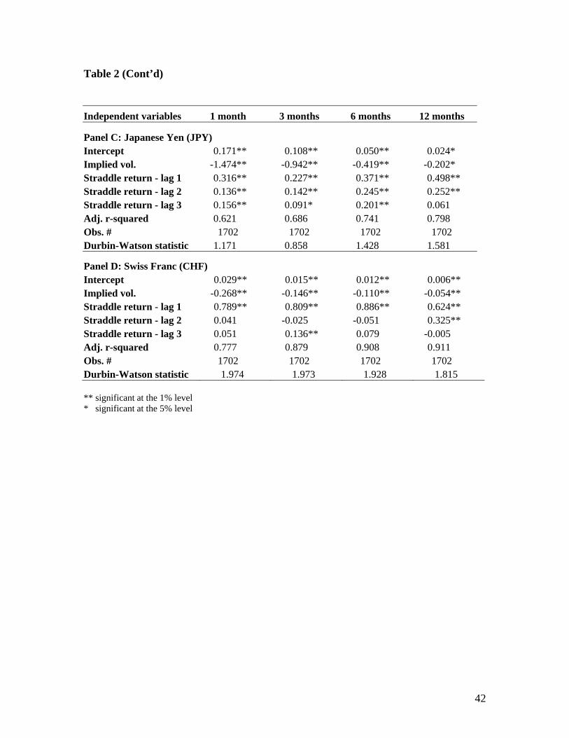
42

Table 2 (Cont’d) Independent variables 1 month 3 months 6 months 12 months

Panel C: Japanese Yen (JPY) Intercept 0.171** 0.108** 0.050** 0.024* Implied vol. -1.474** -0.942** -0.419** -0.202* Straddle return - lag 1 0.316** 0.227** 0.371** 0.498** Straddle return - lag 2 0.136** 0.142** 0.245** 0.252** Straddle return - lag 3 0.156** 0.091* 0.201** 0.061 Adj. r-squared 0.621 0.686 0.741 0.798 Obs. # 1702 1702 1702 1702 Durbin-Watson statistic 1.171 0.858 1.428 1.581

Panel D: Swiss Franc (CHF) Intercept 0.029** 0.015** 0.012** 0.006** Implied vol. -0.268** -0.146** -0.110** -0.054** Straddle return - lag 1 0.789** 0.809** 0.886** 0.624** Straddle return - lag 2 0.041 -0.025 -0.051 0.325** Straddle return - lag 3 0.051 0.136** 0.079 -0.005 Adj. r-squared 0.777 0.879 0.908 0.911 Obs. # 1702 1702 1702 1702 Durbin-Watson statistic 1.974 1.973 1.928 1.815 ** significant at the 1% level * significant at the 5% level

43

Table 3: Non-overlapping straddle returns

For each currency, we construct a non-overlapping monthly series of delta-hedged straddle returns on the 1-month straddles bought at the first trading day of every month in the sample period. Panel A shows the summary statistics for non-overlapping series. Panel B shows the results of estimating this regression:

1 tttt yy εγσα +++= − where yt is the delta-hedged straddle return, and σt is the implied volatility quote. If the volatility risk is priced and has a negative premium, we expect γ to be significant and negative. The sample period is from June 1996 to December 2002 for the British Pound, the Japanese Yen, and the Swiss Franc, and January 1999 to December 2002 for the Euro. British Pound Euro Japan. Yen Swiss Franc Panel A. Summary statistics Obs. # 77 48 77 77 Mean -0.0182 -0.0101 -0.0202 -0.0030 Std. Dev. 0.0541 0.0544 0.0835 0.0731 % of negative 66% 58% 63% 60% Autocorrelation coefficient

Lag 1 -0.1448 -0.1232 0.0746 -0.0976 Lag 2 -0.1504 -0.1380 0.2390 -0.0321 Lag 3 0.0300 0.0948 -0.0518 0.0517 Panel B. regression against implied vol Intercept 0.0359** 0.0531 0.0360 0.0496* Implied vol. -0.4225** -0.4988* -0.4073* -0.5141* Lag 1 0.8969** 0.6944** 0.7660** 0.8611** Adj. r-squared 0.8514 0.5331 0.7548 0.8584 Durbin-Watson 1.8082 2.1030 1.4851 1.7141 ** significant at the 1% level * significant at the 5% level

44

Table 4: Regression of the first difference of delta-hedged straddle return on the first difference of implied volatility This table presents the estimated results for the regression model

332211 ttDtDtDtDDt yyyy εβββσγα +++++= −−− ∆∆∆∆∆ where ty is the delta-hedged return on a delta-neutral straddle bought on date t , ty∆ is the difference between ty and 1−ty , tσ is the volatility quoted for a delta-neutral straddle on date t , and tσ∆ is the difference between tσ and 1−tσ . We include three lagged dependent variables to control for serial autocorrelation. One regression model is estimated for each combination of currency and maturity. The objective is to test the null hypothesis that 0=Dγ .

Independent variables 1 month 3 months 6 months 12 months

Panel A: British Pound (GBP) Intercept 0.0001 0.0001 0.0001 0.0001 ∆ Implied vol. -2.9214** -1.5621** -1.0189** -0.7190** ∆Straddle return – lag 1 -0.1852** -0.2628** -0.3466** -0.2696** ∆Straddle return – lag 2 -0.1163** 0.0135 -0.2859** -0.1839 ∆Straddle return – lag 3 -0.0796** 0.0336 0.0713 0.0096 Obs. # 1701 1701 1701 1701 Adj. r-squared 0.2110 0.2506 0.2337 0.2084 Durbin-Watson statistic 2.1016 2.1082 2.0589 1.9941

Panel B: Euro (EUR) Intercept 0.0000 -0.0001 -0.0001 -0.0001 ∆ Implied vol. -2.6459** -1.6170** -1.1664** -0.8543** ∆Straddle return – lag 1 -0.0633 -0.1109** -0.0835** -0.0370 ∆Straddle return – lag 2 -0.0360 -0.1930* -0.0326 0.0001 ∆Straddle return – lag 3 -0.1699* -0.0833 -0.0082 -0.0457 Obs. # 1023 1023 1023 1023 Adj. r-squared 0.1427 0.2768 0.3114 0.3137 Durbin-Watson statistic 2.0810 1.8912 2.1098 2.0541 ** significant at the 1% level * significant at the 5% level

45

Table 4 (Cont’d) Independent variables 1 month 3 months 6 months 12 months

Panel C: Japanese Yen (JPY) Intercept 0.0000 0.0001 0.0001 0.0000 ∆ Implied vol. -2.4670** -1.4187** -0.8722** -0.4115** ∆Straddle return - lag 1 -0.0546* -0.0225** -0.0923 -0.1223* ∆Straddle return - lag 2 -0.0527 -0.0099 -0.0799 -0.0315 ∆Straddle return - lag 3 -0.0355 -0.0206 -0.0635 -0.0752 Obs. # 1701 1701 1701 1701 Adj. r-squared 0.8831 0.9545 0.8244 0.5919 Durbin-Watson statistic 2.1641 2.3060 2.2903 2.2432

Panel D: Swiss Franc (CHF) Intercept 0.0001 0.0000 0.0000 0.0001 ∆ Implied vol. -2.8374** -1.6060** -1.1459** -0.7615** ∆Straddle return - lag 1 -0.1513** -0.1249** -0.0039 -0.2461** ∆Straddle return - lag 2 -0.0952** -0.1592** -0.1209 -0.0077 ∆Straddle return - lag 3 -0.0208 -0.0883* -0.0476 0.0851 Obs. # 1701 1701 1701 1701 Adj. r-squared 0.1477 0.2950 0.3030 0.3392 Durbin-Watson statistic 2.0398 2.1151 1.9904 2.0218 ** significant at the 1% level * significant at the 5% level

46

Table 5: Pooled regression of the first difference of delta-hedged straddle return on the first difference of implied volatility We pool the delta-hedged straddle returns for four maturities and estimate the following model for each currency

tttt

tttt

t

yyyIIII

IIIIy

εβββσγσγσγσγ

αααα

+∆+∆+∆+∗∆+∗∆+∗∆+∗∆

++++=∆

−−− 332211

12,12126,663,331,11

1212663311

where ty is the delta-hedged return on a delta-neutral straddle bought on date t , ty∆ is the difference between ty and 1−ty , ti ,σ is the quoted volatility for the i -month maturity on date t , tσ∆ is the difference between tσ and 1−tσ , and iI is the indicator variable of an observation for the i -month maturity with i being 1, 3, 6 or 12. We use iα to allow different intercepts at different maturities. Our main focus is on iγ s, which measures the unit delta-hedged straddle return at different maturities. The sample period is from June 1996 to December 2002 for the British Pound, the Japanese Yen, and the Swiss Franc, and January 1999 to December 2002 for the Euro. Currency

Independent variables GBP EUR JPY CHFDummy - 1 month 0.0001 0.0000 0.0000 0.0001 Dummy - 3 months 0.0001 -0.0001 0.0001 0.0000 Dummy - 6 months 0.0001 -0.0001 0.0001 0.0000 Dummy - 12 months 0.0000 -0.0001 0.0000 0.0001 ∆ Implied vol. - 1 month -2.9198** -2.6396** -2.4747** -2.8370** ∆ Implied vol. - 3 months -1.5518** -1.6121** -1.4014** -1.6082** ∆ Implied vol. – 6 months -1.0541** -1.1724** -0.8916** -1.1115** ∆ Implied vol. – 12 months -0.7349** -0.8544** -0.4270** -0.7804** ∆Straddle return - lag 1 -0.2078** -0.0654 -0.0495** -0.1469** ∆Straddle return - lag 2 -0.1198** -0.0423 -0.0439 -0.0994** ∆Straddle return - lag 3 -0.0526 -0.1645* -0.0334 -0.0253 Obs. # 6804 4092 6804 6804 Adj. r-squared 0.2079 0.1509 0.8933 0.1624 Durbin-Watson statistic 2.0964 2.0786 2.2042 2.0451 Wald test for H0: 121 γγ = Statistic 173.8484 81.5774 1703.0080 120.5293 (p-value) (0.00) (0.00) (0.00) (0.00) Wald test for H0: 12631 γγγγ +=+

Statistic 188.4576 96.8067 1863.0928 158.5117 (p-value) (0.00) (0.00) (0.00) (0.00) ** significant at the 1% level * significant at the 5% level

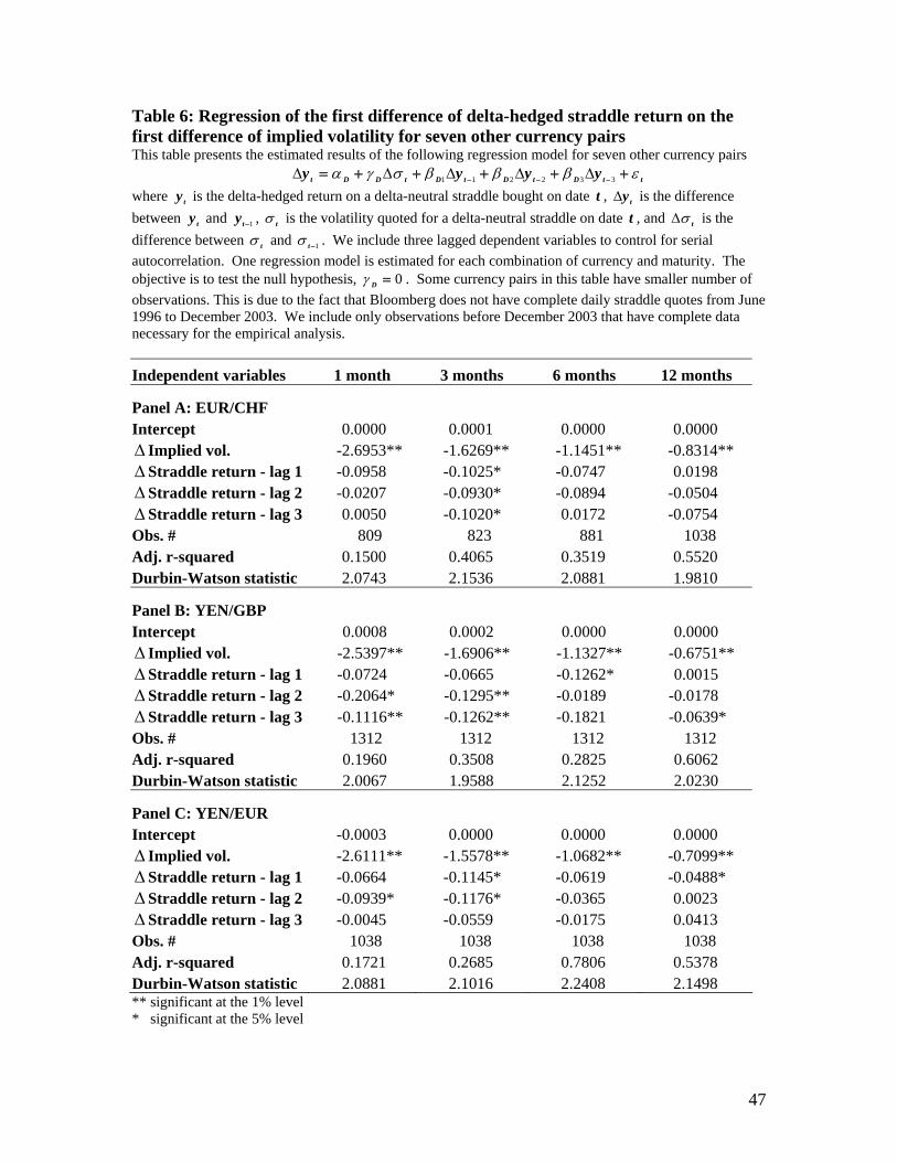
47

Table 6: Regression of the first difference of delta-hedged straddle return on the first difference of implied volatility for seven other currency pairs This table presents the estimated results of the following regression model for seven other currency pairs

332211 ttDtDtDtDDt yyyy εβββσγα +++++= −−− ∆∆∆∆∆ where ty is the delta-hedged return on a delta-neutral straddle bought on date t , ty∆ is the difference between ty and 1−ty , tσ is the volatility quoted for a delta-neutral straddle on date t , and tσ∆ is the difference between tσ and 1−tσ . We include three lagged dependent variables to control for serial autocorrelation. One regression model is estimated for each combination of currency and maturity. The objective is to test the null hypothesis, 0=Dγ . Some currency pairs in this table have smaller number of observations. This is due to the fact that Bloomberg does not have complete daily straddle quotes from June 1996 to December 2003. We include only observations before December 2003 that have complete data necessary for the empirical analysis.

Independent variables 1 month 3 months 6 months 12 months

Panel A: EUR/CHF Intercept 0.0000 0.0001 0.0000 0.0000 ∆ Implied vol. -2.6953** -1.6269** -1.1451** -0.8314** ∆Straddle return - lag 1 -0.0958 -0.1025* -0.0747 0.0198 ∆Straddle return - lag 2 -0.0207 -0.0930* -0.0894 -0.0504 ∆Straddle return - lag 3 0.0050 -0.1020* 0.0172 -0.0754 Obs. # 809 823 881 1038 Adj. r-squared 0.1500 0.4065 0.3519 0.5520 Durbin-Watson statistic 2.0743 2.1536 2.0881 1.9810

Panel B: YEN/GBP Intercept 0.0008 0.0002 0.0000 0.0000 ∆ Implied vol. -2.5397** -1.6906** -1.1327** -0.6751** ∆Straddle return - lag 1 -0.0724 -0.0665 -0.1262* 0.0015 ∆Straddle return - lag 2 -0.2064* -0.1295** -0.0189 -0.0178 ∆Straddle return - lag 3 -0.1116** -0.1262** -0.1821 -0.0639* Obs. # 1312 1312 1312 1312 Adj. r-squared 0.1960 0.3508 0.2825 0.6062 Durbin-Watson statistic 2.0067 1.9588 2.1252 2.0230

Panel C: YEN/EUR Intercept -0.0003 0.0000 0.0000 0.0000 ∆ Implied vol. -2.6111** -1.5578** -1.0682** -0.7099** ∆Straddle return - lag 1 -0.0664 -0.1145* -0.0619 -0.0488* ∆Straddle return - lag 2 -0.0939* -0.1176* -0.0365 0.0023 ∆Straddle return - lag 3 -0.0045 -0.0559 -0.0175 0.0413 Obs. # 1038 1038 1038 1038 Adj. r-squared 0.1721 0.2685 0.7806 0.5378 Durbin-Watson statistic 2.0881 2.1016 2.2408 2.1498 ** significant at the 1% level * significant at the 5% level

48

Table 6 (Cont’d) Independent variables 1 month 3 months 6 months 12 months

Panel D: Australian (AUD) Intercept 0.0000 0.0000 0.0000 0.0000 ∆ Implied vol. -2.5600** -1.5400** -1.0200** -0.9300** ∆Straddle return - lag 1 -0.0974** -0.1463** -0.1287** -0.0257* ∆Straddle return - lag 2 -0.0773* -0.0149 -0.0535 -0.0115 ∆Straddle return - lag 3 -0.0269 -0.0663* -0.0120 -0.0188 Obs. # 1679 1678 1680 1713 Adj. r-squared 0.0853 0.1358 0.1669 0.9415 Durbin-Watson statistic 2.0574 2.0652 2.0914 2.2327

Panel E: Canadian Dollar (CAD) Intercept -0.0009 -0.0003 -0.0001 -0.0002 ∆ Implied vol. -2.9158** -2.2620** -0.8643** -0.7757** ∆Straddle return – lag 1 -0.2000** 0.0638 -0.2799** -0.1132 ∆Straddle return – lag 2 -0.1590** -0.0618 -0.1879** -0.2699 ∆Straddle return – lag 3 0.0005 0.0305 -0.0752 -0.1786 Obs. # 298 168 137 60 Adj. r-squared 0.2663 0.5639 0.5337 0.3782 Durbin-Watson statistic 2.1184 2.2678 2.0147 2.0831

Panel F: Norwegian Kroner (NOK) Intercept -0.0009 0.0002 0.0000 0.0000 ∆ Implied vol. -2.6090** -1.3140** -0.9449** -0.7532** ∆Straddle return – lag 1 -0.2202** -0.2013** -0.1969** -0.1989** ∆Straddle return – lag 2 -0.1640** -0.1552 -0.0545 -0.0650 ∆Straddle return – lag 3 -0.0903* -0.1037 0.0367 -0.0034 Obs. # 463 409 410 855 Adj. r-squared 0.1727 0.3092 0.4749 0.7013 Durbin-Watson statistic 2.0961 2.1529 1.9701 2.3951

Panel G: New Zealand Dollar (NZD) Intercept -0.0013 -0.0001 -0.0001 -0.0001 ∆ Implied vol. -2.6634** -1.4516** -0.8526** -0.6591** ∆Straddle return - lag 1 -0.1802** -0.1473* -0.1472* -0.0613 ∆Straddle return - lag 2 -0.0549 -0.0690 -0.0786 0.0329 ∆Straddle return - lag 3 -0.0318 -0.1491** -0.1151* -0.0855 Obs. # 667 576 504 480 Adj. r-squared 0.2093 0.2595 0.3701 0.4521 Durbin-Watson statistic 2.0985 2.0498 2.2401 1.9519 ** significant at the 1% level * significant at the 5% level

49

Table 7: Pooled regression of the first difference of delta-hedged straddle return on the first difference of implied volatility for seven other currency pairs We pool the delta-hedged straddle returns for four maturities and estimate the following model for seven other currency pairs

tttt

tttt

t

yyyIIII

IIIIy

εβββσγσγσγσγ

αααα

+∆+∆+∆+∗∆+∗∆+∗∆+∗∆

++++=∆

−−− 332211

12,12126,663,331,11

1212663311

where ty is the delta-hedged return on a delta-neutral straddle bought on date t , ty∆ is the difference between ty and 1−ty , ti ,σ is the quoted volatility for the i -month maturity on date t , tσ∆ is the difference between tσ and 1−tσ , and iI is the indicator variable of an observation for the i -month maturity with i being 1, 3, 6 or 12. We use iα to allow different intercepts at different maturities. Our main focus is on iγ s, which measures the unit delta-hedged straddle return at different maturities. Currency

Independent variables EUR/CHF YEN/GBP YEN/EUR Dummy - 1 month 0.0000 0.0008 -0.0003 Dummy - 3 months 0.0001 0.0002 0.0000 Dummy - 6 months 0.0000 0.0001 0.0000 Dummy - 12 months 0.0000 0.0000 0.0000 ∆ Implied vol. - 1 month -2.6865** -2.5426** -2.6094** ∆ Implied vol. - 3 months -1.6384** -1.6866** -1.5646** ∆ Implied vol. – 6 months -1.1471** -1.1307** -1.0664** ∆ Implied vol. – 12 months -0.8205** -0.6564** -0.7170** ∆Straddle return - lag 1 -0.0956* -0.0746 -0.0708* ∆Straddle return - lag 2 -0.0329 -0.1956* -0.0930* ∆Straddle return - lag 3 -0.0101 -0.1153 -0.0097 Obs. # 3551 5248 4152 Adj. r-squared 0.1899 0.2091 0.2073 Durbin-Watson statistic 2.0848 2.0061 2.0905 Wald test for H0: 121 γγ = Statistic 14.4969 51.9282 37.6506 (p-value) (0.00) (0.00) (0.00) Wald test for H0: 12631 γγγγ +=+

Statistic 20.0182 65.2485 52.8223 (p-value) (0.00) (0.00) (0.00) ** significant at the 1% level * significant at the 5% level

50

Table 7 (Cont’d) Currency

Independent variables AUD CAD NOK NZD Dummy - 1 month 0.0000 -0.0009 -0.0009 -0.0013 Dummy - 3 months 0.0000 -0.0003 0.0002 -0.0001 Dummy - 6 months 0.0000 -0.0001 0.0000 -0.0001 Dummy - 12 months 0.0000 -0.0001 0.0000 -0.0001 ∆ Implied vol. - 1 month -2.5600** -2.9134** -2.6085** -2.6600**∆ Implied vol. - 3 months -1.5400** -2.1086** -1.3094** -1.4761**∆ Implied vol. – 6 months -1.0300** -0.8959** -0.9484** -0.8506**∆ Implied vol. – 12 months -0.9000** -0.7963** -0.7393** -0.6393**∆Straddle return - lag 1 -0.1004** -0.1812** -0.2191** -0.1761**∆Straddle return - lag 2 -0.0701* -0.1504* -0.1605** -0.0563 ∆Straddle return - lag 3 -0.0307 -0.0016 -0.0875* -0.0428 Obs. # 6750 663 2137 2227 Adj. r-squared 0.1245 0.2904 0.1985 0.2180 Durbin-Watson statistic 2.0621 2.1378 2.0997 2.1005 Statistic 35.6092 15.7488 45.3234 29.1777 (p-value) (0.00) (0.00) (0.00) (0.00) Wald test for H0: 12631 γγγγ +=+ Statistic 42.3990 31.1340 46.8289 38.6366 (p-value) (0.00) (0.00) (0.00) (0.00) ** significant at the 1% level * significant at the 5% level

51

Table 8: Summary statistics of the delta-hedged straddle return for the post-Asian currency crisis sub-period The U.S. Dollar delta-hedged straddle profit (loss) from holding the dynamically delta-hedged portfolio until maturity is computed by

( ) ( ) ( )( )N

--0, ,1

0

1

0, 1

ττττ ∑∑

−

=

−

=+++ ∆−−−∆−−−=∏

+

N

ntttttt

N

ntttttttt nnnnn

xqrfrxxfxkkxMax

where ƒt is the straddle premium at time t, xt+τ is the currency price at the maturity t+τ, k is the strike price of the straddle, nt∆ is the delta of the long straddle, rt

and qt are the domestic and foreign interest rates. The delta-hedged straddle return is calculated as Πt, t+τ divided by the straddle contract size in U.S. dollars. We annualize the return to make it comparable across maturities. We report summary statistics on the return for four currencies at four standard maturities. For each combination of currency and maturity, the delta-hedged straddle return comprises a time series of one observation on each trading day. We fit an AR(3) process to the time series and test whether the intercept is zero. This is equivalent to a test of whether the mean delta-hedged straddle return is equal to zero. The post-Asian currency crisis sub-period is from July 1999 to December 2002.

Autocorrelation coefficient Partial autocorrelation

coefficient AR(3) Intercept Maturity Obs. #

% of negative return

Sample mean

Sample standard deviation Lag 1 Lag 2 Lag 3 Lag 1 Lag 2 Lag 3 Estimate P-value

Panel A: British Pound (GBP) 1 month 902 70% -0.0213 0.0484 0.846 0.750 0.692 0.846 0.123 0.113 -0.0027 0.00653 months 902 78% -0.0185 0.0223 0.943 0.909 0.883 0.943 0.172 0.105 -0.0009 0.02046 months 902 82% -0.0162 0.0165 0.939 0.893 0.881 0.939 0.087 0.289 -0.0003 0.077912 months 902 82% -0.0133 0.0120 0.926 0.885 0.883 0.926 0.193 0.314 -0.0003 0.0666

Panel B: Euro (EUR) 1 month 902 59% -0.0130 0.0642 0.842 0.731 0.647 0.842 0.077 0.048 -0.0018 0.1117

3 months 902 68% -0.0131 0.0264 0.959 0.927 0.900 0.959 0.091 0.047 -0.0005 0.0674

6 months 902 67% -0.0106 0.0194 0.976 0.957 0.937 0.976 0.096 -0.012 -0.0003 0.0887

12 months 902 64% -0.0093 0.0152 0.986 0.973 0.961 0.986 0.038 0.032 -0.0002 0.0317

52

Table 8 (Cont’d)

Autocorrelation coefficient Partial autocorrelation

coefficient AR(3) Intercept Maturity Obs. #

% of negative return

Sample mean

Sample standard deviation Lag 1 Lag 2 Lag 3 Lag 1 Lag 2 Lag 3 Estimate P-value

Panel C: Japanese Yen (JPY) 1 month 902 59% -0.0138 0.0732 0.878 0.781 0.705 0.878 0.044 0.049 -0.0017 0.16533 months 902 66% -0.0147 0.0363 0.886 0.816 0.745 0.886 0.144 -0.007 -0.0014 0.03856 months 902 82% -0.0155 0.0278 0.803 0.711 0.628 0.803 0.186 0.038 -0.0020 0.081412 months 902 70% -0.0096 0.0211 0.820 0.722 0.579 0.820 0.151 -0.145 -0.0017 0.0093

Panel D: Swiss Franc (CHF) 1 month 902 55% -0.0010 0.0660 0.834 0.720 0.656 0.834 0.081 0.119 -0.0002 0.8726

3 months 902 67% -0.0095 0.0248 0.939 0.902 0.868 0.939 0.172 0.046 -0.0006 0.0376

6 months 902 68% -0.0098 0.0165 0.950 0.915 0.884 0.950 0.125 0.038 -0.0004 0.0090

12 months 902 75% -0.0085 0.0118 0.967 0.950 0.927 0.967 0.238 -0.037 -0.0003 0.0034

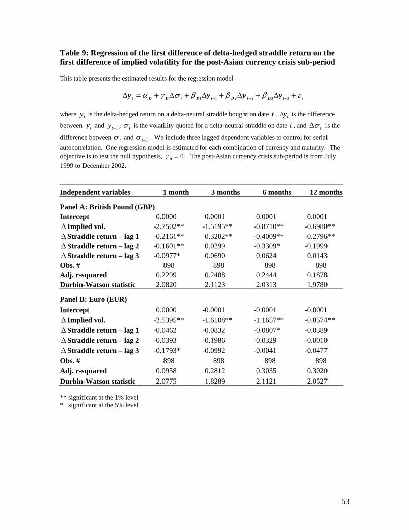
53

Table 9: Regression of the first difference of delta-hedged straddle return on the first difference of implied volatility for the post-Asian currency crisis sub-period This table presents the estimated results for the regression model

332211 ttDtDtDtDDt yyyy εβββσγα +++++= −−− ∆∆∆∆∆

where ty is the delta-hedged return on a delta-neutral straddle bought on date t , ty∆ is the difference

between ty and 1−ty , tσ is the volatility quoted for a delta-neutral straddle on date t , and tσ∆ is the

difference between tσ and 1−tσ . We include three lagged dependent variables to control for serial autocorrelation. One regression model is estimated for each combination of currency and maturity. The objective is to test the null hypothesis, 0=Dγ . The post-Asian currency crisis sub-period is from July 1999 to December 2002.

Independent variables 1 month 3 months 6 months 12 months

Panel A: British Pound (GBP) Intercept 0.0000 0.0001 0.0001 0.0001 ∆ Implied vol. -2.7502** -1.5195** -0.8710** -0.6980** ∆Straddle return – lag 1 -0.2161** -0.3202** -0.4009** -0.2796** ∆Straddle return – lag 2 -0.1601** 0.0299 -0.3309* -0.1999 ∆Straddle return – lag 3 -0.0977* 0.0690 0.0624 0.0143 Obs. # 898 898 898 898 Adj. r-squared 0.2299 0.2488 0.2444 0.1878 Durbin-Watson statistic 2.0820 2.1123 2.0313 1.9780

Panel B: Euro (EUR) Intercept 0.0000 -0.0001 -0.0001 -0.0001 ∆ Implied vol. -2.5395** -1.6108** -1.1657** -0.8574** ∆Straddle return – lag 1 -0.0462 -0.0832 -0.0807* -0.0389 ∆Straddle return – lag 2 -0.0393 -0.1986 -0.0329 -0.0010 ∆Straddle return – lag 3 -0.1793* -0.0992 -0.0041 -0.0477 Obs. # 898 898 898 898 Adj. r-squared 0.0958 0.2812 0.3035 0.3020 Durbin-Watson statistic 2.0775 1.8289 2.1121 2.0527 ** significant at the 1% level * significant at the 5% level

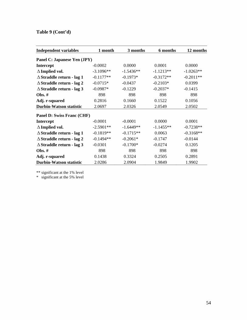
54

Table 9 (Cont’d) Independent variables 1 month 3 months 6 months 12 months

Panel C: Japanese Yen (JPY) Intercept -0.0002 0.0000 0.0001 0.0000 ∆ Implied vol. -3.1096** -1.5436** -1.1213** -1.0263** ∆Straddle return - lag 1 -0.1177** -0.1973* -0.3172** -0.2011** ∆Straddle return - lag 2 -0.0715* -0.0437 -0.2103* 0.0399 ∆Straddle return - lag 3 -0.0987* -0.1229 -0.2037* -0.1415 Obs. # 898 898 898 898 Adj. r-squared 0.2816 0.1660 0.1522 0.1056 Durbin-Watson statistic 2.0697 2.0326 2.0549 2.0502

Panel D: Swiss Franc (CHF) Intercept -0.0001 -0.0001 0.0000 0.0001 ∆ Implied vol. -2.5901** -1.6449** -1.1455** -0.7238** ∆Straddle return - lag 1 -0.1819** -0.1715** 0.0063 -0.3168** ∆Straddle return - lag 2 -0.1494** -0.2061* -0.1747 -0.0144 ∆Straddle return - lag 3 -0.0301 -0.1700* -0.0274 0.1205 Obs. # 898 898 898 898 Adj. r-squared 0.1438 0.3324 0.2505 0.2891 Durbin-Watson statistic 2.0286 2.0904 1.9849 1.9902 ** significant at the 1% level * significant at the 5% level

55

Table 10: Effect of jumps on the delta-hedged straddle return We identify the day on which the daily percentage change in the currency price is two standard deviations away from the mean daily percentage change in our sample period. We examine the delta-hedged straddle returns in the day immediately before or after these price jumps. We do not differentiate between negative and positive jumps because the straddle price is equally sensitive to moves in both directions. The first column reports the number of days when price jumped. Take the British Pound as an example. Between June 3, 1996 and December 31, 2002, 103 days (about 6%) experienced large moves in the U.S. Dollar price of the British Pound in either a positive or a negative direction. Before jumps After jumps Before vs. after # of jumps Mean Median Mean Median Mean Median

Maturity (p-value of

t-test) (p-value of

Wilcoxon test)(p-value of t-test)

(p-value of Wilcoxon test)

(p-value of t-test)

(p-value of Wilcoxon test)

Panel A: British Pound (GBP) 1 month 103 -0.0009 0.0031 -0.0354 -0.0357 0.0345 0.0307 (0.88) (0.89) (0.00) (0.00) (0.00) (0.00)3 months 103 -0.0167 -0.0199 -0.0257 -0.0275 0.0090 0.0078 (0.00) (0.00) (0.00) (0.00) (0.00) (0.00)6 months 103 -0.0155 -0.0150 -0.0188 -0.0194 0.0033 0.0025 (0.00) (0.00) (0.00) (0.00) (0.00) (0.00)12 months 103 -0.0149 -0.0177 -0.0166 -0.0188 0.0017 0.0010 (0.00) (0.00) (0.00) (0.00) (0.10) (0.00)Panel B: Euro (EUR) 1 month 53 0.0242 0.0265 -0.0251 -0.0116 0.0493 0.0442 (0.03) (0.01) (0.01) (0.05) (0.00) (0.00)3 months 53 -0.0102 -0.0071 -0.0206 -0.0201 0.0104 0.0095 (0.00) (0.01) (0.00) (0.00) (0.00) (0.00)6 months 53 -0.0094 -0.0103 -0.0136 -0.0115 0.0042 0.0053 (0.00) (0.00) (0.00) (0.00) (0.00) (0.00)12 months 53 -0.0117 -0.0157 -0.0125 -0.0147 0.0008 0.0014 (0.00) (0.00) (0.00) (0.00) (0.30) (0.24)Panel C: Japanese Yen (JPY) 1 month 82 0.0257 0.0367 -0.0444 -0.0474 0.0701 0.0607 (0.20) (0.06) (0.01) (0.00) (0.00) (0.00)3 months 82 0.0023 -0.0051 -0.0237 -0.0163 0.0259 0.0134 (0.73) (0.84) (0.07) (0.01) (0.03) (0.00)6 months 82 -0.0010 -0.0059 -0.0078 -0.0155 0.0068 0.0071 (0.87) (0.26) (0.17) (0.02) (0.00) (0.00)12 months 82 -0.0079 -0.0108 -0.0109 -0.0121 0.0030 0.0033 (0.01) (0.00) (0.00) (0.00) (0.10) (0.00)Panel D: Swiss Franc (CHF) 1 month 100 0.0353 0.0235 0.0004 -0.0017 0.0349 0.0309 (0.00) (0.00) (0.95) (0.66) (0.00) (0.00)3 months 100 0.0005 0.0003 -0.0067 -0.0112 0.0072 0.0052 (0.87) (0.91) (0.02) (0.01) (0.00) (0.00)6 months 100 -0.0058 -0.0101 -0.0087 -0.0130 0.0030 0.0023 (0.00) (0.00) (0.00) (0.00) (0.00) (0.00)12 months 100 -0.0066 -0.0058 -0.0076 -0.0072 0.0009 0.0006 (0.00) (0.00) (0.00) (0.00) (0.08) (0.07)

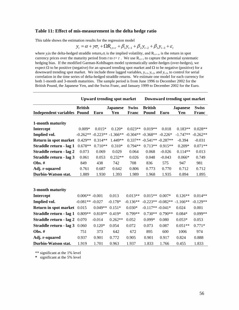
56

Table 11: Effect of mis-measurement in the delta hedge ratio This table shows the estimation results for the regression model

332211, tttttttt yyyRy εβββγσα τ ++++Ω++= −−−+

where ytis the delta-hedged straddle return,σt is the implied volatility, and Rt t+τ, is the return in spot currency prices over the maturity period from t to t+τ . We use Rt t+τ to capture the potential systematic hedging bias. If the modified Garman-Kohlhagen model systematically under-hedges (over-hedges), we expect Ω to be positive (negative) for an upward trending spot market and Ω to be negative (positive) for a downward trending spot market. We include three lagged variables, yt-1, yt-2, and yt-3, to control for serial correlation in the time series of delta-hedged straddle returns. We estimate one model for each currency for both 1-month and 3-month maturities. The sample period is from June 1996 to December 2002 for the British Pound, the Japanese Yen, and the Swiss Franc, and January 1999 to December 2002 for the Euro.

Upward trending spot market Downward trending spot market

Independent variables British Pound Euro

Japanese Yen

Swiss Franc

British Pound Euro

Japanese Yen

Swiss Franc

1-month maturity Intercept 0.009* 0.015* 0.120* 0.023** 0.019** 0.018 0.183** 0.028**Implied vol. -0.262** -0.223** -1.366** -0.304** -0.368** -0.226* -1.747** -0.262**Return in spot market 0.429** 0.314** 1.449** 0.337** -0.541** -0.287** -0.394 -0.031 Straddle return - lag 1 0.678** 0.710** 0.310* 0.794** 0.713** 0.915** 0.209* 0.071**Straddle return - lag 2 0.073 0.069 0.029 0.064 0.068 -0.026 0.114** 0.013 Straddle return - lag 3 0.061 0.053 0.232** 0.026 0.048 -0.043 0.066* 0.749 Obs. # 849 438 742 708 836 575 947 981 Adj. r-squared 0.761 0.687 0.642 0.806 0.773 0.770 0.712 0.712 Durbin-Watson stat. 1.889 1.930 1.393 1.989 1.968 1.935 0.894 1.895 3-month maturity Intercept 0.006** -0.001 0.013 0.013** 0.015** 0.007* 0.126** 0.014**Implied vol. -0.081** -0.027 -0.178* -0.136** -0.223** -0.082** -1.166** -0.129**Return in spot market 0.015 0.049** 0.151* 0.030* -0.117** -0.041* 0.024 0.001 Straddle return - lag 1 0.809** 0.818** 0.419* 0.799** 0.730** 0.790** 0.084* 0.099**Straddle return - lag 2 0.070 -0.014 0.262** 0.052 0.099* 0.080 0.053* 0.053 Straddle return - lag 3 0.060 0.120* 0.054 0.072 0.073 0.087 0.051** 0.771* Obs. # 751 373 642 672 895 600 1006 974 Adj. r-squared 0.937 0.901 0.772 0.905 0.901 0.917 0.824 0.888 Durbin-Watson stat. 1.919 1.701 0.963 1.937 1.833 1.766 0.455 1.833 ** significant at the 1% level * significant at the 5% level

57

0.0

0.10

0.20

0.30

1 month 3 months 6 months 12 months

British Pound

0.0

0.10

0.20

0.30

1 month 3 months 6 months 12 months

Euro

0.0

0.10

0.20

0.30

1 month 3 months 6 months 12 months

Japanese Yen

0.0

0.10

0.20

0.30

1 month 3 months 6 months 12 months

Swiss Franc

Figure 1: Distribution of implied volatility quotes for the whole sample period This figure shows the boxplots of the daily implied volatility quotes for 1-month, 3-month, 6-month and 12-month at-the-money straddle between June 1996 and December 2002 for British Pound, Japanese Yen, and Swiss Franc, and between January 1999 and December 2002 for Euro.

58

Figure 2: Time series plot of implied volatility quotes This figure shows the daily implied volatility for the 3-month at-the-money straddle for the British Pound, the Japanese Yen and the Swiss Franc between June 1996 and December 2002. The two vertical dash lines indicate the start and the end of the Asian currency crisis period.

Bristish Pound 3 month Implied Volatility

0

5

10

15

20

25

3-Ju

n-96

3-D

ec-9

6

3-Ju

n-97

3-D

ec-9

7

3-Ju

n-98

3-D

ec-9

8

3-Ju

n-99

3-D

ec-9

9

3-Ju

n-00

3-D

ec-0

0

3-Ju

n-01

3-D

ec-0

1

3-Ju

n-02

3-D

ec-0

2

Mean 8.47%

Japanese Yen 3 month Implied Volatility

05

10152025

3-Ju

n-96

3-De

c-96

3-Ju

n-97

3-De

c-97

3-Ju

n-98

3-De

c-98

3-Ju

n-99

3-De

c-99

3-Ju

n-00

3-De

c-00

3-Ju

n-01

3-De

c-01

3-Ju

n-02

3-De

c-02

Mean 11.96%

Swiss Franc 3 month Implied Volatility

05

10152025

3-Ju

n-96

3-De

c-96

3-Ju

n-97

3-De

c-97

3-Ju

n-98

3-De

c-98

3-Ju

n-99

3-De

c-99

3-Ju

n-00

3-De

c-00

3-Ju

n-01

3-De

c-01

3-Ju

n-02

3-De

c-02

Mean 10.9%

Bristish Pound 3 month Implied Volatility

0

5

1015

20

25

3-Ju

n-96

3-D

ec-9

6

3-Ju

n-97

3-D

ec-9

7

3-Ju

n-98

3-D

ec-9

8

3-Ju

n-99

3-D

ec-9

9

3-Ju

n-00

3-D

ec-0

0

3-Ju

n-01

3-D

ec-0

1

3-Ju

n-02

3-D

ec-0

2

Mean 8.47%

Japanese Yen 3 month Implied Volatility

05

10152025

3-Ju

n-96

3-De

c-96

3-Ju

n-97

3-De

c-97

3-Ju

n-98

3-De

c-98

3-Ju

n-99

3-De

c-99

3-Ju

n-00

3-De

c-00

3-Ju

n-01

3-De

c-01

3-Ju

n-02

3-De

c-02

Mean 11.96%

Swiss Franc 3 month Implied Volatility

05

10152025

3-Ju

n-96

3-De

c-96

3-Ju

n-97

3-De

c-97

3-Ju

n-98

3-De

c-98

3-Ju

n-99

3-De

c-99

3-Ju

n-00

3-De

c-00

3-Ju

n-01

3-De

c-01

3-Ju

n-02

3-De

c-02

Mean 10.9%

59

0.0

0.10

0.20

0.30

1 month 3 months 6 months 12 months

British Pound

0.0

0.10

0.20

0.30

1 month 3 months 6 months 12 months

Euro

0.0

0.10

0.20

0.30

1 month 3 months 6 months 12 months

Japanese Yen

0.0

0.10

0.20

0.30

1 month 3 months 6 months 12 months

Swiss Franc

Figure 3: Distribution of implied volatility quotes in the post-Asian currency crisis sub-period This figure shows the boxplots of the daily implied volatility quotes for 1-month, 3-month, 6-month and 12-month at-the-money straddle between July 1999 and December 2002 for all four currencies.