the utilization and effect of information transfer in
TRANSCRIPT

THE UTILIZATION AND EFFECT OF INFORMATION TRANSFER IN
AUDITING: AMONG AUDIT ENGAGEMENT TEAMS, AUDIT CLIENTS, AND
SUPPLY CHAIN PARTNERS
By CHENG YIN
A dissertation submitted to the
Graduate School – Newark
Rutgers, The state University of New Jersey
In partial fulfillment of requirements
For the degree of
Doctor of Philosophy
Graduate Program in Management
Written under the direction of
Dr. Alexander Kogan
and approved by
Dr. Miklos A. Vasarhelyi
Dr. Helen Brown-Liburd
Dr. Rajendra Srivastava
Newark, New Jersey
May 2018

© [2018]
CHENG YIN
ALL RIGHTS RESERVED

ii
ABSTRACT OF THE DISSERTATION
THE UTILIZATION AND EFFECT OF INFORMATION TRANSFER IN
AUDITING: AMONG AUDIT ENGAGEMENT TEAMS, AUDIT CLIENTS, AND
SUPPLY CHAIN PARTNERS
By CHENG YIN
Dissertation Director: Dr. Alexander Kogan
This dissertation consists of three essays that examine the utilization and effect of
information transfer in auditing practice. Specially, I investigate two types of information
transfer: information sharing and information diffusion. In information sharing, the
information is transferred purposefully to target agents or spread within pre-selected groups.
Unlike information sharing, information diffusion occurs when information is created,
delivered and propagated by any active nodes within certain groups without purposeful
directions.
In the first essay, I explore the possibilities of information sharing between audit
engagement teams and demonstrate the benefits of doing this, under the assumption that
the same audit firm serves multiple clients competing in the same industry. I introduce a
number of sharing schemes for utilizing contemporaneous accounting information from
peer companies without violating clients’ confidentiality. To satisfy different levels of
privacy protection, I propose different sharing schemes by utilizing auditors’ self-
generated expectations, and find that auditors can achieve comparable levels of benefits

iii
from only sharing self-generated estimation residuals (errors) with that from sharing
predicted or actual accounting numbers, both in estimation accuracy and in error detection
performance. To satisfy stricter privacy concerns, I also propose a scheme based on sharing
categorical information derived from prediction errors. Finally, I use Borda counts to
analyze how the choice of the best model changes depending on the cost of errors within
different experimental settings.
The second essay examines the effect on audit quality of “horizontal” information
diffusion among audit clients within geographic industry clusters. I define the geographic
industry clusters as the agglomerations of firms from the same industry, located in the same
metropolitan statistical area (MSA). Based on a significant negative effect of geographic
industry clusters on audit quality, I also investigate the reasons that foster such quality gap.
As predicted, the quality difference is more pronounced for firms with stronger local
connection measured by the number of local industry competitors sharing the same auditor.
In addition, I also find that the geographic industry clusters have a positive effect on audit
pricing and the existence of local connection intensifies such impact. Overall, the evidence
suggests that due to the lower communication cost in the geographic industry clusters,
clients are more likely to learn questionable accounting practices and form alliances to
negotiate with auditors and convince them to accept questionable accounting practices. For
fear of losing clients, auditors charge clients within the clusters higher audit fees to
compensate the raising litigation risks, especially those clients with local connections.
The third essay investigates the effect of “vertical” information diffusion between
supply chain partners and emphasizes the role of auditors in reducing information

iv
asymmetry and sustaining business relationships. I examine the association between
auditor reputation of suppliers and the duration of supply chain relationships and find
empirical evidence that a poor reputation for the supplier’s auditor increases the likelihood
of customer-supplier relationship termination. However, that effect will be mitigated if
customers and suppliers are located close to each other or if they share common auditors.
Furthermore, suppliers who remediate the problem by switching from low reputation
auditors to high reputation auditors will send positive signals to customers, which will
decrease the likelihood of a relationship breakdown in the following year.

v
ACKNOWLEDGMENTS
This dissertation would not have been accomplished without the help and support
of my committee members, my colleagues, and my family. I appreciate this great
opportunity to convey my gratitude to them with all my sincerity.
First of all, I would love to express my respect and appreciation to my advisor Dr.
Alexander Kogan for his rigorous training, unlimited patience and pertinent suggestions.
The weekly meetings that we spent together, provided me with great experiences. I am very
grateful to Dr. Miklos A. Vasarhelyi for his generous support and constant care. I am deeply
thankful to Dr. Helen Brown-Liburd for her valuable feedback in auditing research and Dr.
Rajendra Srivastava for serving on the committee and providing precious insight for my
future career. Also, I would like to express my gratitude to Dr. Dan Palmon for his trust,
recognition, protection and encouragement. Without his help, I would not know where to
go. Last but not least, I would like to thank Dr. Bikki Jaggi for his extraordinary guidance
in accounting studies.
I was lucky to have friends and colleagues with warm heart and love. My special
thanks go to my treasured friends and colleagues: Xin Cheng, Yinan Yang, Feiqi Huang,
Yulin Sun, Lingyi Zheng, Xuan Peng, Yifei Chen, Fujun Tang, Xianjue Wang, He Li, Ting
Sun, Qiao Li, Zhaokai Yan, Yue Liu, Tiffany Chiu, and Yunsen Wang.
Finally, I express my greatest thanks to my family members for their support and
love.

vi
TABLE OF CONTENTS
ABSTRACT OF THE DISSERTATION ............................................................... ii
ACKNOWLEDGMENTS ...................................................................................... v
CHAPTER 1: INTRODUCTION ........................................................................... 1
CHAPTER 2: PRIVACY-PRESERVING INFORMATION SHARING WITHIN
AN AUDIT FIRM............................................................................................................... 8
2.1 Introduction ................................................................................................... 8
2.2 Background and Sharing Schemes.............................................................. 17
2.2.1 Background .......................................................................................... 17
2.2.2 Sharing Schemes .................................................................................. 20
2.3 Evaluation of Proposed Designs ................................................................. 33
2.3.1 Data ...................................................................................................... 33
2.3.3 Model ................................................................................................... 39
2.2.4 Methodologies...................................................................................... 42
2.4 Validation Results ....................................................................................... 51
2.4.1 Estimation Accuracy ............................................................................ 51
2.4.2 Error Detection..................................................................................... 59
2.4.3 The Choice of the Best Model ............................................................. 63
2.5 Concluding Remarks ................................................................................... 66

vii
CHAPTER 3: GEOGRAPHIC INDUSTRY CLUSTERS AND AUDIT QUALITY
........................................................................................................................................... 69
3.1 Introduction ................................................................................................. 69
3.2 Literature Review and Hypotheses Development ....................................... 73
3.3 Research Design.......................................................................................... 79
3.3.1 Measures .............................................................................................. 79
3.3.2 Model Specifications ........................................................................... 83
3.4 Sample Selection and Descriptive Statistics ............................................... 86
3.4.1 Sample.................................................................................................. 86
3.4.2 Descriptive Statistics and Univariate Tests.......................................... 87
3.4.3 Pearson Correlation Matrix .................................................................. 90
3.5 Empirical Results ........................................................................................ 93
3.5.1 Main Results ........................................................................................ 93
3.6 Robustness Checks.................................................................................... 103
3.6.1 Concerns on Geographic Proximity between Auditor and Client ..... 103
3.6.2 Restatements ...................................................................................... 105
3.7 Conclusion ................................................................................................ 107
CHAPTER 4: AUDITOR REPUTATION AND THE DURATION OF
CUSTOMER-SUPPLIER RELATIONSHIPS ............................................................... 109
4.1 Introduction ............................................................................................... 109

viii
4.2 Literature Review and Hypothesis Development ..................................... 116
4.3 Research Design........................................................................................ 124
4.3.1 Sample................................................................................................ 124
4.3.2 Measures of Auditor Reputation ........................................................ 125
4.3.3 Model Specifications ......................................................................... 127
4.4 Results ....................................................................................................... 133
4.4.1 Descriptive Statistics .......................................................................... 133
4.4.2 Multivariate Results ........................................................................... 134
4.5 Additional Analysis .................................................................................. 141
4.6 Conclusion ................................................................................................ 146
CHAPTER 5: CONCLUSION ........................................................................... 148
APPENDICIES ................................................................................................... 151
Appendix A. .................................................................................................... 151
Appendix B. .................................................................................................... 153
REFERENCES ................................................................................................... 154
SUPPLEMENTARY APPENDICES ................................................................. 167
Appendix A. .................................................................................................... 167
Appendix B. .................................................................................................... 171
Appendix C. .................................................................................................... 175

ix
Appendix D. .................................................................................................... 180
SUPPLEMENTARY MATERIALS .................................................................. 185
Section A. ........................................................................................................ 186
Section B. ........................................................................................................ 202
Section C. ........................................................................................................ 219
LIST OF TABLES
Table 1. The Summary of Sharing Schemes with Three Levels of Privacy ............. 30
Table 2. Descriptive Statistics - Sample from 1991–2015 ....................................... 34
Table 3. An illustration of the Peer Selection Criteria .............................................. 37
Table 4. Specification of Models .............................................................................. 40
Table 5. The Ranking Result for 5 Prediction Intervals, with 15 Pairs of Parameters
........................................................................................................................... 49
Table 6. The Preference Ballots for a Certain Company in the Considered 15
Scenarios ........................................................................................................... 50
Table 7. The Evaluation of Prediction Accuracy in Estimating Revenue Account . 54
Table 8. The Evaluation of Prediction Accuracy in Estimating Cost of Goods Sold 57
Table 9. The Evaluation of Error Detection .............................................................. 61

x
Table 10. The Change of Best Models According to Different Magnitudes of Errors
........................................................................................................................... 64
Table 11. The Change of Best Models According to Different Cost Ratios ............ 65
Table 12. Descriptive Statistics ................................................................................. 88
Table 13. Pearson Correlation Matrix ....................................................................... 91
Table 14. Geographic Industry Cluster and Audit Quality ....................................... 94
Table 15. Local Connection and Audit Quality ........................................................ 96
Table 16. Geographic Industry Cluster and Audit Fee ............................................. 99
Table 17. Local Connection and Audit Fees ........................................................... 101
Table 18. Robustness Checks – Geographic Proximity .......................................... 104
Table 19. Robustness Checks - Restatement .......................................................... 105
Table 20. Descriptive Statistics ............................................................................... 133
Table 21. The Association between Auditor Reputation and Supply Chain
Relationship .................................................................................................... 135
Table 22. The Impact of Information Sharing on the Association between Auditor
Reputation and Supply Chain Relationship .................................................... 137
Table 23. The Impact of Auditor Dismissal on the Association between Auditor
Reputation and Supply Chain Relationship .................................................... 140
Table 24. Whether Suppliers with Major Customers Tend to choose Auditors with
Higher Reputations ......................................................................................... 142

xi
Table 25. Robustness Checks ................................................................................. 144

1
CHAPTER 1: INTRODUCTION
In the realm of accounting, an “information transfer” occurs when a value-relevant
information (e.g. earnings announcement) for one firm affects the expectations (e.g. stock
prices) for other firms, whose economic prospects are interrelated (e.g. production process,
customer group) with each other (Foster 1981; Ettredge and Richardson 2003) For
example, if one firm announces bad news (e.g. usually lower than expected earnings), that
firm is likely to experience negative CAR (cumulative abnormal returns). Further, similar
firms (e.g. competitors within the same industry or supply chain partners) are likely to
experience simultaneous abnormal returns. Such simultaneous abnormal returns can be
negative due to industry commonalities or be positive because of competitive shifts
between rival firms (Kim, Lacina and Park 2008). Prior studies provide evidence on
information transfers from earnings announcements (Firth 1976; Foster 1981; Clinch and
Sinclair 1987; Han and Wild 1990; Freenab and Tse 1992; Ramnath 2002; Thomas and
Zhang 2008), management forecasts (Baginski, 1987; Han, Wild and Ramesh, 1989; Pyo
and Lustgarten, 1990; Kim, Lacina and Park 2008), accounting standards harmonization
(Wang 2014) and even the case of hacker attacks (Ettredge and Richardson 2003).
However, there are fewer studies that investigate the utilization and effect of
information transfer in auditing practice for two possible reasons. First, in current regimes
(Rule 1.700.001.01, AICPA), auditors are forbidden to directly utilize “transferred”
information (e.g. contemporaneous accounting information from other clients audited by
other engagement teams) from other engagement teams under the requirements of client
confidentiality. Second, prior studies focus on the role of auditors as accounting assurance

2
providers rather than as information transfer repositories/ intermediators (Bae et al. 2017;
Fiolleau et al. 2013). Therefore, to bridge such research gaps, this dissertation is going to
investigate the utilization and effect of information transfer in auditing practice, among
audit engagement teams, audit clients, and supply chain partners. Specially, in the
following three chapters, I am planning to discuss two types of information transfer:
information sharing and information diffusion.
In information sharing, the information is transferred purposefully to target
receivers or spread among pre-selected group members. This procedure may include
mediators, usually unrealted third parties, to guarantee the independence of interventions.
Studies of information transfer usually seek to identify two prime factors: the firms with
interrelated economic prospects and the information events that are value-relevant for firms
directly affected (Ettredge and Richardson 2003). According to the above two criteria, the
firms with interrelated economic prospects were identified as peer firms. An illustrative
value-relevant information event can be the account estimation during analytical
procedures, since prior studies show that peer companies data can be utilized to improve
auditing effectiveness through analytical procedures (Hoitash et al. 2006). However, these
studies assume the availability of a database repository used to enable data sharing among
auditors. The feasibility of creating such a repository is in question due to audit clients’
privacy concerns. Hence, my second chapter (first essay) is trying to answer the question
of how to set up a practical privacy-preserving framework for sharing information among
auditors without violations of clients’ confidentiality. I introduce a number of sharing
schemes for utilizing contemporaneous accounting information from peer companies
without violating clients’ confidentiality and observe significant improvements associated

3
with sharing contemporaneous information from peer companies, both in estimation
accuracy and error detection performance. To satisfy different levels of privacy protection,
I propose different sharing schemes by utilizing auditors’ self-generated expectations, and
find that auditors can achieve comparable levels of benefits from only sharing self-
generated estimation residuals (errors) with that from sharing predicted or actual
accounting numbers, both in estimation accuracy and in error detection performance. To
satisfy stricter privacy concerns, I also propose a scheme based on sharing categorical
information derived from prediction errors. Finally, I use Borda counts to analyze how the
choice of the best model changes depending on the cost of errors within different
experimental settings.
After investigating the utilization of information sharing among audit engagement
teams, I explore the effect of information diffusion among audit clients within the same
industry. Unlike information sharing, information diffusion is the process where
information is created, delivered, and propagated among any active nodes (agents) with no
purposeful directions. At the beginning, information diffuses sequentially from some
particular information source, such as a group of nodes (agents) outside the group or other
information intermediators such as mass media or thorough “word of mouth”. For example,
investors often spend lots of time discussing investment strategies with other investors (Liu
et al. 1997). With the development of online social networks, investors may create, discuss
and spread information through social media, such as Facebook and Twitter (Guille et al.
2013). This kind of social activity tends to become a form of group pressure, which has
influence on investors’ original expectations. Prior literature documents various research
questions such as how to identify influential spreaders (Li et al. 20142014), how to infer

4
the underlying spreading cascade (Gomez et al. 2010), how to predict specific diffusion
process by learning past diffusion traces (Galuba et al. 2010), and how to detect the popular
topics (Kempe et al. 2003).
In this dissertation, I focus on the information diffusion among audit clients
especially clients from the same industry and MSA1 (industry clusters) and believe the
diffusion effects are more prevalent within geographic industry clusters due to both closer
industrial and geographic distances. As suggested by Kewei Hou (2007), firms within an
industry compete in the same product market and their operating decisions reflect strategic
interaction between them. As the industry experiences expansions and contractions, these
firms’ growth opportunities and investing and financing decisions are highly interrelated.
Additionally, the engagements and negotiations with auditors can be treated as one of
value-relevant information events. Thus, it is worthy to investigate the effect of information
diffusion among audit clients on audit quality and audit pricing.
The third chapter (second essay) of the dissertation examines whether there is a
difference in audit quality between firms within “geographic industry clusters” and those
firms outside clusters, using a large sample of audit client firms from 2000 to 2015.
Consistent with prior literature, I define the geographic industry clusters as the
agglomerations of firms from the same industry located in the same metropolitan statistical
area (MSA) (Almazan et al. 2010). Further, based on a significant negative effect of
1 A geographic entity defined by the federal Office of Management and Budget for use by federal statistical
agencies, based on the concept of a core area with a large population nucleus, plus adjacent communities
having a high degree of economic and social integration with that core.
https://factfinder.census.gov/help/en/metropolitan_statistical_area_msa.htm

5
geographic industry clusters on audit quality, I also investigate the reasons that foster such
quality gap. As predicted, the quality difference is more pronounced for firms with stronger
local connection measured by the number of local industry competitors sharing the same
auditor. In addition, I also find that the geographic industry clusters have a positive effect
on audit pricing and the existence of local connection intensifies such impact. Overall, the
empirical evidence suggests that due to the lower communication cost in the geographic
industry clusters, clients are more likely to learn questionable accounting practices and
form alliances to negotiate with auditors and convince them to accept questionable
accounting practices. For fear of losing clients, auditors charge clients within the clusters
higher audit fees to compensate the rising litigation risks, especially those clients with local
connections.
Most studies investigate the information transfer within the same industry, named
“horizontal” information transfer, but Olsen et al. (1985) find “vertical” information
transfer occurs among supply chain partners as well. The information diffusion over supply
chains may occur when either suppliers or customers (un) obtain value-relevant
information about their collaborators. This information may change their expectations on
future prospects and business cooperation of their supply chain partners. Following this
research stream, I extend my research scope to investigate the effect of “vertical”
information diffusion over supply chains and emphasize the importance of auditors in
aiding management decision making and sustaining business relationships. The fourth
chapter discusses the importance of auditors in reducing information asymmetries and
sustaining supply chain relationships and studies the association between auditor reputation
and the duration of customer-supplier relationships. I argue that the reliability of auditors’

6
opinions influences customers’ confidence in suppliers’ financial reporting and operating
performance, which affects the level of information asymmetry and the quality of
information sharing between these supply chain partners.
The auditor’s reputation, measured by the number of announcements of
restatements, is a publicly available proxy for customers’ perceived level of trust in their
collaborations with their suppliers (Swanquist and Whited 2015). Investigating the
hypothesis that customers and suppliers may view transaction conditions more favorably
and sustain longer relationships if the customers are assured of the quality of information
that was audited by trusted auditors (Kinney 2000), we provide empirical evidence that a
poor reputation for the supplier’s auditor increases the likelihood of customer-supplier
relationship termination. However, that effect will be mitigated if customers and suppliers
are located close to each other or if they share common auditors. Furthermore, suppliers
who remediate the problem by switching from low reputation auditors to high reputation
auditors will send positive signals to customers, which will decrease the likelihood of a
relationship breakdown in the following year. The empirical findings emphasize the
significant role of auditors and the importance of auditor reputation in maintaining supply
chain relationships.
To summarize, the structure of this dissertation is as follows: in Chapter 2, I propose
several information sharing schemes that explore the benefits and possibilities of utilizing
information transfer (sharing) in auditing practice. Chapter 3 studies the effect of
“horizontal” information diffusion among audit clients by investigating the influence of
geographic industry clusters on audit quality. Chapter 4 discusses the effect of “vertical”

7
information diffusion among supply chain partners and emphasizes the important role of
auditors in reducing information asymmetries and sustaining supply chain relationships.
The last chapter provides some concluding remarks.

8
CHAPTER 2: PRIVACY-PRESERVING INFORMATION SHARING WITHIN
AN AUDIT FIRM
2.1 Introduction
The well-publicized audit failures of Enron, WorldCom and others have brought to
the forefront the issue of audit effectiveness. The emergence of data-driven technologies
and methodologies, and the big data context, put more emphasis on developing and refining
innovative audit data analysis techniques. A promising family of such techniques utilizes
information sharing in the auditing process, especially information from similar companies
subjected to the common financial environment (macro-economic cycle, market
conditions, etc.). Such peer companies also experience similar non-financial shocks.
Therefore, comparisons of their results can provide valuable information for auditors. Prior
studies show that peer companies data can be utilized to improve auditing effectiveness
through analytical procedures. Specially, Hoitash, Kogan and Vasarhelyi (2006) introduce
an approach for selecting peers and perform tests to examine the contribution of peers’
information to the performance of analytical procedures. However, this study assumes the
availability of a database repository used to enable data sharing among auditors. The
feasibility of creating such a repository is in question due to audit clients’ privacy concerns.
Hence, an important question left unanswered is how to design a practical privacy-
preserving artifact for sharing information among auditors without violations of clients’
confidentiality.

9
This chapter fills this research gap and follows the paradigm of design science1 to
create effective analytical procedures that enable auditors to share client information within
an audit firm in a privacy-preserving manner, under the assumption that the same audit
firm serves multiple clients competing in the same industry. The rationale for this
assumption is based on the theory of audit firm industry specialization2 (Mayhew et al.
2003, Chan et al. 2004). In particular, our approach is more instructive for those audit firms
which follow a cost minimization strategy and gain market share by providing service to a
large portion of companies within the same industry (Cahan, Debra and Vic 2011).
The design of artifacts is not exempt from natural laws or behavioral theories but
relies on existing kernel theories (Walls et al. 1992; Markus et al. 2002). The foundation
for our design is based on the usefulness of peer firm data. To be specific, many previous
studies (Healy and Palepu 2007; Stickney et al. 2007; Damodaran 2007) have showed the
advantages of using peer firms as a benchmark3 and the methodologies of choosing peers
(Hoitash et al. 2006; Minutti-Meza, M. 2013; De Franco et al. 2015). In more relevant
studies, prior literature has extensively examined the importance of information transfer
1 The design-science paradigm is fundamentally a problem-solving paradigm and has its roots in engineering
and the sciences of the artificial (Simon 1996). 2 This theory asserts that audit firms differentiate themselves from other competitors to maximize
profitability. Developing industry specific knowledge can allow auditors to satisfy clients’ demands and earn
profits due to economies of scale. Therefore, audit firms make costly investments to train specialists in
specific industries and differentiate themselves from others in terms of assurance services (Hogan and Jeter
1999, Dunn and Mayhew 2000). 3 For instance, financial analysts use peer firms to support their valuation multiples, earnings forecasts and
overall stock recommendations (De Franco et al. 2011). Investment managers use peer firms in structuring
their portfolios (Chan et al. 2007). Peer firms are used by compensation committees in setting executive
compensation (Albuquerque 2009; Albuquerque et al. 2013), in determining valuation multiples (Bhojraj and
Lee 2002), as well as by auditors in conducting analytical procedures (Hoitash et al. 2006; Minutti-Meza
2013).

10
and industry expertise in providing high-quality audits4. With the development of data-
driven methodologies in analytical procedures since 1980s, researchers have proposed
numerous ways5 to boost the performance of analytical procedures. The extant literature
has provided sufficient evidence to believe that incorporating peer-based industrial
contemporaneous data could improve the performance of analytical procedures.
Since peer companies typically have the same fiscal years, and audit opinions have
to be formulated before the disclosure of financial statements, contemporaneous data from
peer companies are not publicly available. The data availability problem becomes a hurdle
in the way of obtaining the benefits from incorporating contemporaneous information.
Thus, many previous studies only used company specific current data plus publicly
available data but did not use contemporaneous data from peer companies6. A reasonable
solution to this problem would be sharing contemporaneous data from peer companies
audited by the same audit firm. The current regime (Rule 1.700.001.01) requires auditors
to protect clients’ data confidentiality but does not forbid auditors from using clients’ data
to improve their audit quality, as stated in Rule 1.700.001.02.). Moreover, in circumstances
4 For instance, they suggest that knowledge of the industry may increase audit quality (Balsam et al. 2003;
Krishnan 2003; Reichelt and Wang 2010), improve the accuracy of error detection (Solomon et al. 1999;
Owhoso et al. 2002), enhance the quality of auditors’ risk assessment (Taylor 2000; Low 2004), and optimize
the allocation of audit resources and audit efforts (Low 2004). 5 They start to use higher data frequency (Wild 1987; Dzeng 1994), apply more sophisticated statistical
models (Dugan et al. 1985; Pany 1990; Leitch and Chen 2003), and consider multiple companies in similar
industries (Lev 1980; AICPA 1988; Wheeler and Pany 1990; Allen 1992) as well as multi-location data
(Allen et al. 1999). 6 In Hoitash et al. (2006), they find that the inclusion of contemporaneous data from peer companies does not
always outperform benchmark model when other contemporaneous variables are included. This finding
implies that the inclusion of contemporaneous data could always improve the estimation accuracy, and thus
sharing the prediction that contains contemporaneous data could provide more information than sharing the
historical public available data alone. Therefore, this is the reason why we explore the possibilities of
obtaining the benefits from sharing contemporaneous data instead of from utilizing public available data.

11
where the auditor specializes in a specific industry, the auditor may use clients’ data to
develop plausible expectations7 (Guy and Carmichael 2002). As Gal (2008) suggested,
auditors have responsibilities to determine the precise definition of sensitive data, the
timeliness of information released and the appropriateness of technologies used for
information protection. Therefore, we believe that if the auditor can guarantee no
disclosure or leakage of confidential information during the sharing process, it is valuable
to study a possible implementation of a privacy-preserving information sharing scheme
among the auditors in the same audit firm.
To address the client privacy preservation needs articulated above, we first
theoretically develop a so-called “generic sharing scheme” by introducing a third party
(e.g., the central office / headquarters of accounting firms) as a control unit responsible for
generating, assigning and passing aggregated/modified information derived from clients’
private data in an anonymous setting.
Next, to alleviate the concerns related to the impairment of third parties’
independence, we propose a modified generic sharing scheme that avoids the involvement
of third parties. The modified generic sharing scheme trades off some efficiency of the
generic sharing scheme to enable participants to exchange information between each other
following a pre-defined path.
Further, to mitigate the concerns of raw data exposure and enable different levels
of privacy protection, we offer a number of information sharing schemes as alternatives
7 For example, gross margin percentage, other income statement ratios, and receivable and inventory turnover
ratios.

12
that utilize auditors’ self-generated accounting expectations of numerical and categorical
nature. Specifically, we first propose a prediction-based expectation sharing scheme in
which the auditors share the standardized self-generated predicted values instead of clients’
raw data. A residual-based expectation sharing scheme is proposed to satisfy even more
stringent privacy requirements. It allows the auditors to share the standardized self-
generated prediction errors (residuals) instead of prediction values to further reduce the
possibilities of raw data exposure. Additionally, as an extension of the residual-based
sharing scheme, we develop a categorical sharing scheme based on the information derived
from prediction residuals. In this sharing scheme, the auditors convert the numerical
prediction residuals into two pieces of categorical information: the sign of prediction errors
and the level of deviations and share either one of these two variables or both of them.
Based on how similar the shared information is to the raw data, we categorize the
proposed levels of sharing from high to low: the high-level sharing scheme (sharing the
actual clients’ data by utilizing the generic/modified generic sharing scheme), the medium-
level sharing scheme (the prediction-based expectation sharing scheme), the low-level
sharing scheme (the residual-based expectation sharing scheme),the categorical sharing
scheme with both categorical variables, and the categorical sharing scheme with only one
categorical variable.
Design science is well recognized in the IS (Information Systems) literature and
addresses research through the building and evaluation of artifacts that are developed to
meet the identified business needs (Von et al. 2004). Unlike behavioral and empirical
paradigms that are commonly accepted in accounting research, design science aims to

13
determine how a new developed artifact works instead of why the artifact works. In other
words, it puts more emphasis on the utility not the truth of the artifacts. As argued by prior
literature (Simon 1996 and Von et al. 2004), the research paradigms are inseparable and
the contribution of a certain research should be evaluated by its practical implications not
methodologies. Thanks to the mathematical basis, design science allows many types of
quantitative evaluation methodologies, such as optimization proofs, analytical simulation,
and quantitative comparisons with alternative/ previous designs. In this chapter, we use
commonly accepted designs and metrics to evaluate our sharing schemes not only in terms
of estimation accuracy but also in error detection performance in comparison with
competing artifacts. For simplicity, we test the case of “overestimating revenue” and the
case of “underestimating cost of goods sold” as illustrations8.
In the evaluation phase, we use ten representative industries that contained the
largest number of firms from 1991-2015 using 4-digit SIC codes. Since the disaggregated
monthly data performed better in analytical procedures than did the quarterly data, we
interpolate our quarterly data to monthly data. Adapting from Hoitash et al. (2006), we use
the simple auto-regression model that contains both last year public available information
and current year contemporaneous data as the benchmark model. In order to rigorously
simulate the real practice, we impose a constraint that peer firms need to be audited by the
8 In practice, auditors provide assurance on management assertions in the financial statements and verify the
occurrence of transactions related to assets, revenues, liabilities, and expenses. Usually, managers may have
incentives to overestimate their assets and revenues and underestimate their liabilities and expenses to report
inflated profits. However, accounting literature (e.g. Kross et al. 2011, Ma et al. 2017) also provides extensive
evidence that managers have strong incentives to meet earnings expectations and manage earnings downward
to 0 in order to obtain benefits from discretionary accruals.

14
same auditor in the current year, resulting in a large reduction in our sample9. Later, to
investigate the applicability and generalizability of our proposed sharing schemes, we
remove such strict peer selection criteria and increase the number of industries from ten to
twenty, as presented in the Supplementary Appendix A.
First, we compare the MAPEs (mean absolute percentage errors) of all competing
prediction models: the original model, the actual-sharing model, the prediction-sharing
model, and the error-sharing model and categorical-sharing models. We expect the MAPE
will significantly decrease from the original model to other sharing models. If, at the same
time the MAPE is at a comparable level among sharing models, it will show that the
improvement of prediction accuracy by incorporating peer companies’ information can be
attained by sharing auditors’ self-generated information during the estimation process. In
this manner, the clients’ confidentiality can be protected completely by only sharing
auditors’ estimation adjustment errors without utilizing any clients’ accounting numbers.
Moreover, if the MAPE generated by fine-tuned categorical sharing models, is at a
comparable level with higher level sharing models, it provides auditors a more conservative
option to gain the benefits of sharing without violating confidentiality. To verify that our
results are not affected by extreme outliers, we not only tabulate the mean of the MAPE,
but also provide the median of the MAPE. Additionally, because of the loss of information,
the validation performance of the categorical sharing model with only one categorical
variable may suffer, compared to other peer models.
9 The sample shrinkage is consistent with prior literature that investigates the effect of sharing common
auditors between suppliers and customers on audit quality (Johnstone, Li and Luo 2014).

15
Next, we discuss the error detection performance by comparing the original model and
the sharing models. Specially, we compare the error detection performance between the
original model, the three sharing models with different privacy levels and the four
categorical models with separately tuned parameters. A simulation approach known as
“error seeding” is used to compare the anomaly detection capabilities of different models.
In our experiment, we added artificial errors10 to the original values and checked whether
the model could detect the data had been polluted. In the context of our research, the error
detection capability of models is measured as the cost of errors11. In addition, taking the
randomness of choosing contaminated observations into account, we test the impact of the
magnitude of contaminated errors ranging from 5% to 1%, repeat the error seeding
procedure ten times and use the average level as the evaluation to generalize our results,
reduce the selection bias and achieve the robustness of results.
In order to investigate how the choice of the best model changes depending on different
experimental settings, we compare the total cost of errors for different models varying five
different cost ratios, three magnitudes of errors, and five different prediction intervals. We
adapt the Borda count voting method to determine the most suitable model for each
company based on preference ballots with different parameter pairs.
Our analysis shows a new way of increasing prediction accuracy through sharing self-
generated estimations/ residuals among auditors serving the same industry within an audit
firm. In this way, the auditors can benefit without sharing any client raw information, and
10 The magnitude of errors is determined by the magnitude of original values, e.g., 2% of account receivables. 11 The cost of errors can be calculated using three metrics: the numbers of false negative and false positive
errors and the magnitude of the cost ratio between the two types of errors.

16
naturally not violate confidentiality constraints. In addition, we also show that the peer-
based sharing models have superior error detection over the original model and more
interestingly, the low-level sharing scheme in which the auditors only share the estimation
residuals (errors), turns out comparable performance with the medium-level and high-level
sharing schemes in which auditors will share their estimations and actual data respectively.
Moreover, the evaluation results show that the so-called categorical sharing scheme can
achieve a comparable improvement in audit analytical procedures with fine-tuned
thresholds. Finally, in the comparison of the model performances of error detection, we
observe that the best model is usually the mixed categorical information-sharing model that
shares both the sign and the level of deviations of prediction errors. The best model
selection remains relatively stable when we put enough weight on the occurrence of false
negatives.
This study adds to the literature in the following four ways. First, to our best
knowledge, this research is the first to explicitly utilize a design science paradigm in
auditing literature to solve the problem of information sharing among auditors within an
audit firm. We extend and transform Hotaish et al. (2006) theoretical design into a practical
implementation by showing that the self-generated expectation sharing schemes with
properly tuned parameters can achieve similar prediction performance as the actual data
sharing schemes, and under these settings, the auditors can easily realize the benefits of
sharing peer information without violating client confidentiality. Second, our evaluation
evidence supports the conclusion that these improvements are not limited to more accurate
predictions but also result in more effective error detections. Thus, when auditors within
an audit firm have peer clients, utilizing self-generated expectation sharing schemes will

17
result in achieving better audit quality through suitably parameterized audit analytical
procedures in a privacy-preserving manner. Finally, our design of the peer-based analytical
procedures enables auditors to achieve better prediction performance and error detection
without violating clients’ confidentiality, demonstrates the possibility of sharing data
among auditors, and encourages the regulators to reconsider the interaction between
auditors to achieve better auditing results while still preserving clients’ information
security. Finally, our proposed artifacts well satisfy auditors’ different demands of privacy
with extremely low cost by sharing their self-generated aggregated information. It is to be
expected that the adoption of these methods across different industries will reduces the cost
of adoption, implementation, as well as the learning curve.
The remainder of this chapter is organized as follows. Section 2 provides the
background on information sharing during the audit process and describes different sharing
schemes based on different data privacy demands. Section 3 describes the evaluation of
proposed designs including the research questions, the data, the model specifications, and
the methodologies used in our validation tests. The validation tests themselves are
summarized in Section 4. A discussion of the results and some concluding remarks are
presented in Section 5.
2.2 Background and Sharing Schemes
2.2.1 Background
During the auditing process, the auditors can request nearly any information about
their clients. Under the standard confidentiality contract clauses, the auditor must guarantee
that disaggregated information of the client cannot be exchanged, leaked or sold to other

18
individuals or institutions, even to the auditors working in the same audit firm but assigned
to different engagements. We consider hypothetical scenarios designed to model the
practical problems occurring in public accounting firms related to the challenge of privacy-
preserving information sharing between the auditors within the same firm.
The current legal regime requires the auditors to protect clients’ data but does not
prevent the auditors from using these proprietary data for their own analyses. Specifically,
Rule 700.001.01 (previously Rule 301) of the American Institute of Certified Public
Accountants (AICPA) Code of Professional Conduct (2015) states that “a member in a
public practice shall not disclose any confidential client information without specific
consent of the client”. However, current rules do not restrict auditors from using clients’
data to improve their audits, as stated in Rule 700.001.02. In fact, AU section 329.05 states
that, “Analytical procedures involve comparisons of recorded amounts, or ratios developed
from recorded amounts, to expectations developed by the auditor. The auditor develops
such expectations by identifying and using plausible relationships that are reasonably
expected to exist based on the auditor's understanding of the client and of the industry in
which the client operates.” Additionally, there is anecdotal evidence suggesting that
national offices of large public accounting firms use data from a pool of companies in the
same industry as a benchmark for other companies (Hoitash et al. 2006). Moreover,
auditors need to make sure that clients’ confidential information is not disclosed in the
work papers of another client because such information may be subpoenaed in the future.
As noted in Rule 1.700.100, the member’s disclosure of confidential client information in
compliance with a validly issued and enforceable subpoena or summons would not violate
Rule 1.700.001. However, the disclosure of another company’s private information (such

19
as name, sales and purchases) may potentially violate Rule 1.700.090 12 and Rule
1.700.01013.
Recently, a stream of literature investigated the impact of sharing common auditors
on corporate decisions (e.g. Johnstone, Li and Luo 2014; Cai et al. 2016; Dhaliwal et al.
2016; Bae, Gil Soo, et al. 2017). For example, Cai et al. (2016) take a purely empirical
approach to investigate how sharing auditors can reduce deal uncertainty between
participants and bypass the ethical question of sharing clients’ information within an audit
firm. Further, Dhaliwal, et al. (2016) point out a flow of information between bidders and
targets and argue that in order to maintain the relationship between a client and large
acquisition clients, auditors may intend to connect target firms with acquirers and bias the
information to acquiring firms. These studies imply the existence of sharing information
between auditors within the same audit firm and put spotlight on the ethical issues of
protecting clients’ confidential information in auditing practice. Thus, it is urgent and
necessary to emphasize the importance of data privacy while utilizing clients’ information
to improve audit quality.
The cryptology technologies such as public or secret-key encryption (e.g. Bellare
et al. 2001; Boneh et al. 2004) and zero knowledge authentication (e.g. Blum, Feldman and
Micali 1988) were well documented in the IS (Information Security) literature. However,
12 Rule 1.700.090: The member’s disclosure of a client’s name would not violate the “Confidential Client
Information Rule” [1.700.001] if disclosure of the client’s name does not constitute the release of confidential
client information 13 Rule 1.700.010: When a member provides professional services to clients that are competitors, threats to
compliance with the “Confidential Client Information Rule” [1.700.001] may exist because the member may
have access to confidential client information, such as sales, purchases, and gross profit percentages of the
respective competitors.

20
these technologies do not help auditors to share peer data without leaking clients’
information, simply because once the auditors use their private (or shared secret) key to
decrypt the encrypted data, the client’s data is revealed. Another stream of privacy
preserving data mining technologies which can blindly pool and analyze data (e.g. Vaidya
and Clifton 2002, 2003), seems to be a potential solution. However, in audit analytical
procedures, the goal is to improve the estimation power of a specified model for a certain
audit client not an improved industry model by pooling all peer data together.
It is reasonable to consider the possibility of utilizing contemporaneous peer
information by subject matter experts working in the national offices of auditing firms who
can run analytical procedures at the request of the engagement teams and communicate the
results to the engagement team without disclosing the actual data of peer clients competing
in the same industry and thus conceivably avoiding privacy rules violations. However,
based on our personal communications with some Big Four partners, this solution is not
feasible. In fact, if audit engagement teams consult with national office specialists and
obtain their help in analyzing their clients’ data, those specialists are considered to be
temporary members of the engagement team for the duration of the consultation. Therefore,
the same privacy rules apply to these specialists and prevent them from utilizing yet
undisclosed peer competitors’ data in their work for the engagement team.
2.2.2 Sharing Schemes
A generic sharing scheme
As discussed above, auditors are strictly forbidden from leaking any client-owned
data outside the engagement team without explicit consent of their clients. A potential way

21
to deal with the barriers of confidentiality is to share aggregated / modified information
derived from clients’ private data. Thus, the main challenge of sharing information among
engagement teams is to aggregate/ modify the information from clients’ data and transfer
from one engagement team to another without any sensitive disclosures. The function of
disguising, aggregating, and passing data can be controlled by a reliable third party.
The objective of developing a generic sharing scheme is to provide the auditors
with a privacy-preserving data aggregation technique. The basic idea can be described in
the following four steps: add noise to self-owned raw data (e.g., actual accounting numbers,
predictions or residuals produced by regression models), share thus contaminated data with
other engagement teams auditing peer companies, sum up the contaminated data received
from others, and reduce the pre-announced total noise (announced and assigned before
sharing). To be more specific, we provide a simple example below.
Figure 1. The Generic Sharing Scheme: An Example
In this example, A represents an auditor (engagement team) engaged with a client C, F represents the
national office of the audit firm of A, and X, Y and Z are peer companies (and their audit engagement
teams) selected in the current year for client C (engagement team A). In step 1, A passes its last year’s
revenue multiplied by a large number to F. In step 2, F passes a random split of the large number
received from A to X, Y and Z separately. In step 3, A receives the sum of private contaminated
1
A F
X
Y
Z
A
2 3

22
An engagement team of client “A”, whose peers are companies X, Y and Z in the
current year, sends its last year revenue 𝑅𝑡−1 multiplied with a large number M to the
national office of its audit firm “F” that acts as a trusted third party, and requests F to split
the product randomly into the number of parts equal to the number of peers. In this case,
since there are three peer companies for client A, the number of parts equals to three. To
accomplish that, F generates three random parameters (𝛼𝑋 , 𝛼𝑌, 𝛼𝑍) and calculates the ratio
of each parameter to their total sum, to guarantee that the resulting ratios add up to 1.
Specifically, F passes 𝑅𝑡−1 ∗ 𝑀 ∗𝛼𝑋
𝛼𝑋+𝛼𝑌+𝛼𝑍, 𝑅𝑡−1 ∗ 𝑀 ∗
𝛼𝑌
𝛼𝑋+𝛼𝑌+𝛼𝑍 and 𝑅𝑡−1 ∗ 𝑀 ∗
𝛼𝑍
𝛼𝑋+𝛼𝑌+𝛼𝑍 to the engagement teams of peer companies X, Y and Z respectively. Next, the
engagement teams of X, Y and Z add the numbers received from F to their self-owned data
(e.g., current year’s revenue 𝑅𝑡). After the engagement teams of X, Y and Z pass thus
contaminated information back to the engagement team of A, it calculates the aggregated
information (the sum of revenues of peer companies) by deducting the known amount
𝑅𝑡−1 ∗ 𝑀 from 𝑅𝑡𝑋 + 𝑅𝑡
𝑌 + 𝑅𝑡𝑍 + 𝑅𝑡−1 ∗ 𝑀 ∗ (
𝛼𝑋
𝛼𝑋+𝛼𝑌+𝛼𝑍+
𝛼𝑌
𝛼𝑋+𝛼𝑌+𝛼𝑍+
𝛼𝑍
𝛼𝑋+𝛼𝑌+𝛼𝑍).
In this sharing scheme, the privacy of information from X, Y and Z is guaranteed
by adding untraceable noise to the sensitive data. The term “untraceable” requires that the
proposed noise (e.g., last year revenue) should be multiplied by a very large number (M).
If the account balance of revenue is a small number, then adding noise of the same
information from X, Y and Z and subtracts the known self-generated large number to get the
aggregation of private information from X, Y and Z.

23
magnitude may be too weak to protect a larger account balance of peer companies14.
Further, the split ratios are randomly chosen from a uniform distribution between 0 and 1
so that one (or more) ratios could be much smaller than the others. In this case, the
protection will not work either since the added noise becomes too small to provide
significant contamination to the original number. Therefore, the proposed scheme uses a
very large number (say, 1,000,000) to multiply the revenue account by, and the privacy of
peer companies is preserved.
The generic sharing scheme has at least three possible weaknesses. First, this
scheme can only provide privacy protection in the probabilistic sense. In some extremely
rare circumstances, some of the generated random numbers can be so small, that the
contamination will be insufficient to protect the original data. Second, the scheme works
only if the client has more than one peer in the current year. In fact, there are existing
examples of companies having only one peer in a certain year, thus invalidating this
assumption of the information protection scheme. Third, the involvement of third parties
may pose ethical issues that can potentially compromise their reliability. Additionally, in
this generic sharing scheme, it is hard to vary the levels of privacy needed according to a
dynamic (data-driven) demand for privacy protection in audit practice. Therefore, to satisfy
stricter privacy concerns, one has to respond to the challenge of how to eliminate the
involvement of third parties, to reduce the exposure of actual data and to provide multiple
selections of the levels of privacy.
14 For example, assume A’s last year revenue is 0.2 million dollars but the revenues of peer companies X, Y
and Z are more than 10 million dollars. In this scenario, the protection fails because the actual revenues of
peer companies can be extracted by simply ignoring the digits after the decimal point.

24
A modified generic sharing scheme
As we discussed above, the generic sharing scheme utilizes a third party. Since the
involvement of third parties may cause ethical/operating concerns15, we propose a modified
generic sharing scheme that relies on the participation of auditors themselves rather than
the centralized information collection mechanism held by third parties. The basic idea can
be presented as follows.
For company X, with its peer companies Y and Z, they first agree on a pre-defined
information exchange path that starts from X, passes through Y and Z and goes back to X.
To protect X’s actual data, auditor A of company X randomly selects a large enough
amount 𝜀𝑥 as the noise, adds it to X’s original account number 𝑁𝑥, and then passes the sum
(𝜀𝑥 + 𝑁𝑥) to auditor B who is engaged with company Y. Because 𝜀𝑥 is large enough to hide
the relatively small actual number, auditor B has no need to add an additional amount but
to add client Y’s original number 𝑁𝑌 to the amount received from A. Then B passes the
new amount (𝜀𝑥 + 𝑁𝑥 + 𝑁𝑌 ) to the participant C, who is the auditor of company Z.
Similarly, for C, it is impossible to infer the actual numbers of companies X and Y from
the received amount. Next, C adds client Z’s actual number 𝑁𝑧 and sends the total back to
A. Auditor A finally receives the total (𝜀𝑥 + 𝑁𝑥 + 𝑁𝑌 + 𝑁𝑧), reduces the known amount 𝜀𝑥,
divides it by 3 and gets the mean of the numbers from companies X, Y and Z. In the last
step, the privacy of client Y and Z is guaranteed because auditor A only knows the sum of
15 The involvement of third parties may lead to some concerns, such as the independence of execution, the
authentication of assignment and the potential concurrent conflict.

25
𝑁𝑌 + 𝑁𝑧 by reducing the known amount 𝜀𝑥 + 𝑁𝑥 but has no idea how to split this amount
and get the individual numbers of companies Y and Z respectively.
The choice of the large number 𝜀𝑥 would be critical in this sharing scheme. For
example, if we choose 10003 as the noise and the actual number of X is only 56.27, the
addition of the noise and the actual number will be 10059.27. Then, company Y can easily
reduce 10000 and get a very close estimate of 59.27. In this case, the “effective” noise
amount is actually 3, which is definitely not a large enough number to provide reasonable
protection for company X’s sensitive information. A better way is to estimate the
reasonable interval of the sensitive data, for instance, [20,100], then randomly choose a
number from the interval and add this number to the sensitive data. For example, we choose
39.12 from this interval and add to 56.27. It becomes impossible for company Y to guess
the actual number of company X from the received number 95.39. Similarly, in the final
step, the privacy of company Y and Z can be protected since the actual number from
company Y is a proper noise for the actual data from company Z and vice versa, assuming
that company Y and Z are peer companies.
The modified sharing scheme enables auditors to share information without the third
parties, trading off the efficiency of the generic sharing scheme. In the generic sharing
scheme, clients X, Y and Z just need to upload their own encrypted data directly to the
third party without any inter-connections. However, in the modified generic sharing
scheme, the process of information sharing relies on the inter-connections between
participants X, Y and Z. In particular, the “single round” data exchange in the generic
sharing scheme is replaced by the “multiple rounds” in the modified generic sharing

26
scheme. Consequently, the “multiple rounds” of exchange may lead to a higher probability
of data breach. Especially, when the chosen noises in the multiple rounds are extremely
similar, the sensitive data are likely to be decoded. For instance, the auditor of company Z
has access to the addition 𝜀1 + 𝑁𝑥 , 𝜀2 + 𝑁𝑦 , and 𝜀3 + 𝑁𝑥 + 𝑁𝑦 after several rounds of
exchanging. If the noises satisfy the relationship like 2 𝜀3 = 𝜀1 + 𝜀2, then company Z can
easily infer the noise 𝜀3 by adding 𝜀1 + 𝑁𝑥 and 𝜀2 + 𝑁𝑦 together and reducing 𝜀3 + 𝑁𝑥 +
𝑁𝑦. This potentially causes serious data leaking problems. Thus, to reduce the likelihood
of such failures, the participants need to change the way of selecting errors in each round
by applying different distributions, utilizing multiple discontinuous intervals without
overlaps, and utilizing other ways of reinforcing the otherness/ complexities of noise.
In summary, in the generic or modified generic sharing scheme, auditors can gather
the aggregated actual contemporaneous firm-specific information from their peer
companies with privacy controls16. In order to eliminate the size effects on firm-specific
information, auditors can standardize the sharing information themselves in advance. For
example, for company X, after engagement team A receives the standardized aggregated
mean of actual value (z𝑡_𝐵 + z𝑡_𝐶) / 217 from its peer companies Y and Z, the auditor A
can add it as an independent variable in an actual sharing model M𝑎, an auto regression
model: Y𝑡 = 𝛼 + 𝛽1𝑌𝑡−12 + 𝛽2𝑋𝑡 + 𝛽3IND_ACTUAL𝑡 + 𝜀𝑡 , where Y𝑡 is the estimation
account of interest and IND_ACTUAL𝑡 equals (z𝑡_𝐵 + z𝑡_𝐶) / 2 .
16 The privacy control may collapse when participants collude with each other. 17 The value z is the standardized score for clients’ real data.

27
Expectation sharing schemes
Since the generic/modified generic sharing scheme only provides privacy
protection in the probabilistic sense, it is still risky to exchange clients’ actual data.
Therefore, we propose to share auditors’ self-generated expectations instead of clients’ raw
data to attenuate clients’ privacy concerns about raw data exposure.
The auditors’ self-generated expectations, based on both historical data as well as
non-public contemporaneous data, contain the firm-specific information that may improve
analytical procedures for all peer companies. The type of the expectations can vary from
numerical numbers to categorical judgements or from predicted account values to
unexplained residuals. The aggregated auditors’ self-generated expectation is an
informative proxy that captures the contemporaneous industrial information in the current
year.
The logic of the expectation sharing scheme is that, by sharing the self-generated
expectations, auditors may both benefit from information advantages of non-public
contemporaneous data as well as avoid violating clients’ confidentiality, simply because in
this sharing scheme, there is no raw clients’ data exchanged.
First, we introduce a prediction-based expectation sharing scheme as follows.
Assume company X, Y and Z are assigned to different engagement teams A, B and C
respectively in the current year T. Based on prior years’ (T-1) sales and growth numbers,
Y and Z were selected as X’s peer companies. Engagement teams A, B and C estimate the
account of interest first, based on their clients’ provided contemporaneous data combined
with the historical audited data, independently. Since A, B and C are serving as auditors in

28
the same audit firm, it is possible that they choose the same estimation model, for example,
an auto regression model M𝑜 (original model): Y𝑡 = 𝛼 + 𝛽1𝑌𝑡−12 + 𝛽2𝑋𝑡 + 𝜀𝑡 . In this
scheme, the auditors use previous three years (T-3, T-2, and T-1) data to estimate the
original prediction model M𝑜, based on the rolling window approach. Then they plug in
the fourth year (the current year T) data to predict the fourth year’s account number Y�� . To
avoid the impact of company size on the peer average, a standard score is calculated for
each participants X, Y and Z by their assigned auditors A, B and C, as follows: 𝑧 =y−μ(y)
σ(y)
, where y represents a monthly number18 generated by account balance, and the mean and
the standard deviation of the monthly numbers calculated over the previous twelve months.
Next, auditor A collects standardized prediction values z𝑡_�� and z𝑡_�� from B and C and
adds the average of standardized value IND_PREDICT𝑡 = (z𝑡_𝐵 + z𝑡_��)/2 as an
independent variable in the prediction sharing model M𝑝 : Y𝑡 = 𝛼 + 𝛽1𝑌𝑡−12 + 𝛽2𝑋𝑡 +
𝛽3IND_PREDICT𝑡 + 𝜀𝑡.
Being more conservative, auditors may still feel risky to share the prediction values.
To eliminate such concerns, we propose a residual-based expectation sharing scheme,
which shares the prediction residuals (actual value minus predicted value) among auditors.
The residuals are likely to contain useful abnormal information that is not captured in the
original estimation model, such as the direction or the magnitude of the errors between the
actual value and the auditors’ prediction value. In the accounting literature, there are
18 In previous studies, disaggregated monthly data performed better in analytical procedures than did
quarterly data (Wild 1987; Chen and Leitch 1998; Cogger 1981; Knechel 1988; Dzeng 1994). Therefore, we
use monthly observations instead of yearly/quarterly data in our experiment.

29
numerous studies utilizing abnormal accruals (discretionary accruals) based on Jones
model (1991). The abnormal accrual is a regression residual usually used as a proxy for
disclosure quality and a signal of earnings management (Klein et al. 2002, Kothari et al.
2005). Similarly, in the auditing literature, there are a number of papers (Eshleman et al.
2013, Blankley et al. 2012, Choi et al. 2010) discussing the informativeness of “abnormal
audit fees”, the regression residuals produced by audit fee models. Therefore, utilizing the
residuals as supplementary contemporaneous information is a reasonable choice.
To be specific, consistent with the prediction-based expectation sharing scheme,
instead of collecting the standardized prediction values, auditor A collects the standardized
mean of errors IND_ERROR𝑡 = (𝜀𝑡_𝐵 +𝜀𝑡_𝐶 ) / 2 from B and C, where the errors 𝜀𝑡 are
calculated by using the holdout data Y𝑡 (the fourth year data) minus predicted value of the
fourth year Y��. Then auditor A adds the mean of errors IND_ERROR𝑡 as an independent
variable in the error sharing model M𝑒: Y𝑡 = 𝛼 + 𝛽1𝑌𝑡−12 + 𝛽2𝑋𝑡 + 𝛽3IND_ERROR𝑡 +
𝜀𝑡.
The design of the prediction/ residual-based expectation sharing scheme allows for
different levels of privacy. The level of privacy is the opposite to the level of sharing. For
example, sharing the actual data under the generic/modified generic sharing scheme
provides the highest level of sharing but the lowest level of privacy, since the actual number
can be breached due to improper sharing. However, in the prediction/ residual-based
expectation sharing scheme, the auditors only have access to the average of aggregated
predictions/ prediction errors, which can be considered as far less risky exposure compared
to the actual data. Based on how similar the shared information is to the raw numbers, we

30
categorize the proposed levels of sharing from high to low: the high-level sharing scheme
(sharing the actual clients’ data by utilizing the generic/modified generic sharing scheme),
the medium-level sharing scheme (the prediction-based expectation sharing scheme), and
the low-level sharing scheme (the residual-based expectation sharing scheme). Again, as
we mentioned before, the auditors can only utilize one of the medium-level and low-level
sharing schemes, since utilizing both of them is equal to utilizing the high-level sharing
scheme with no privacy protections. The three levels of sharing schemes are summarized
as follows:
Table 1. The Summary of Sharing Schemes with Three Levels of Privacy
Since dummy (categorical) variables are relativey less informative than numerical
(continuous) variables, utilizing such variables will further reduce potential exposure.
Thus, to enhance privacy protection, the low-level sharing scheme can be modified to
protect privacy even better through sharing only categorical information derived from
residuals instead of sharing the residuals themselves. More specifically, the shared
“expectation” information consists of two dummy variables: the sign of prediction errors
and the level of deviations.
Privacy Levels Peer Sharing Model
Low Level 𝜀𝑖≠𝑗
Medium Level y𝑝
High Level 𝑦𝑖 , 𝑖 ≠ 𝑗
For the low-level sharing scheme, auditors will add standardized estimation residuals 𝜺𝒊≠𝒋 from peer
companies as an independent variable; For medium-level sharing scheme, auditors will add standardized
prediction ��𝒑 from peer companies as an independent variable; For high-level sharing scheme, auditors
will add standardized real accounting numbers 𝒚𝒊, 𝒊 ≠ 𝒋 as an independent variable.

31
The sign of prediction errors provides an indication of overestimation or
underestimation based on peer firms’ contemporaneous experience and helps to modify
prediction models in the right direction. If the sign of prediction errors is positive
(negative), it implies auditors have overestimated (underestimated) the account balance.
The level of deviation is a measure of how much the actual number deviates from the
prediction. It is categorized based on a certain threshold: if the deviation (absolute value of
prediction errors) is less than the standard error of prediction times a predefined parameter,
the level of deviation equals zero, but if the deviation is larger than the threshold, the level
of deviation is one. Intuitively, the value of the threshold may significantly affect the
effectiveness of the level of deviation. Specifically, if the value of the threshold is too large,
most observations will have the level of deviation equal to zero, adding no value to
improving the performance of the prediction model. On the contrary, if the value of the
threshold is too small, most observations will have the level of deviation equal to one, also
resulting in minimal effect on the performance of the sharing model. Thus, the threshold
has to be properly chosen to improve the performance of the sharing models.
Extending the illustrations presented above, consider companies X, Y and Z as the
participants in the sharing scheme. In the categorical sharing scheme, the auditors use both
historical and contemporaneous data to estimate the prediction model M𝑜 using the method
discussed above. Rather than collecting the standardized mean of errors from peer
companies, auditor A of company X collects the sign of prediction errors and the level of
deviations from other auditors B and C (within the same audit firm), who are engaged with
peer companies Y, and Z, respectively. The sign of prediction errors and the level of
deviations are both dummy variables. For instance, if auditor B overestimates the revenue

32
with a large deviation, the data shared will be (1, 1). On the contrary, if auditor C
underestimates the revenue with a small deviation, the sharing will be (0, 0). Then auditor
A calculates the aggregated information (average) based on the collected information from
companies Y and Z and adds it as an independent variable that captures the auditors’
prediction adjustments, to improve the performance of analytical procedures. In such
manner, the categorical sharing model will be either M𝑠: Y𝑡 = 𝛼 + 𝛽1𝑌𝑡−12 + 𝛽2𝑋𝑡 +
𝛽3IND_SIGN𝑡 + 𝜀𝑡 (sharing the sign of prediction errors) or M𝑙: Y𝑡 = 𝛼 + 𝛽1𝑌𝑡−12 +
𝛽2𝑋𝑡 + 𝛽3IND_DEVIATION𝑡 + 𝜀𝑡 (sharing the level of deviation). Additionally, it is
reasonable to expect that sharing both the sign of prediction errors and the level of
deviations from peer companies will provide more information than sharing only one of
them. Thus, the model with two categorical variables is expected to outperform the other
two categorical information sharing models. Specifically, the auditors add both IND_SIGN𝑡
and IND_DEVIATION𝑡 in the sharing model, creating a “mixed” categorical information
sharing model M𝑚 : Y𝑡 = 𝛼 + 𝛽1𝑌𝑡−12 + 𝛽2𝑋𝑡 + 𝛽3IND_SIGN𝑡 + 𝛽4IND_DEVIATION𝑡 +
𝜀𝑡.
The categorical expectation sharing schemes preserve more privacy than those sharing
schemes based on numerical data, but these sharing scheme has disadvantages as well. For
a particular firm that has only one peer in the current year, the sharing model will be
reduced to the original model when the peer firm underestimates the account balance with
a small deviation within a certain threshold. Thus, the performance of this sharing scheme
will be downward biased (worse than expected). In addition, a Boolean variable only
contains relatively small amount of information derived from residuals thus resulting in

33
significant reduction in estimation accuracy. The more the loss of information, the poorer
the performance will be. However, as discussed above, sharing both categorical variables
derived from residuals with a fine-tuned threshold may provide a comparable good result
to the other sharing models.
2.3 Evaluation of Proposed Designs
2.3.1 Data
Data preparation
For the purposes of evaluation, twenty industries that contained the largest number
of firms and experienced varying sales growth rates from 1991–2015 were initially selected
using 4-digit SIC codes. The way of choosing industries ensures a good representativeness
of the various economic sectors. For example, the selected industries include the Steel
Works & Blast Furnaces industry (Standard Industrial Classification [SIC] 4911) that
experienced on average 4.86 percent annual growth during the sample period, and the
Pharmaceutical Preparations industry (SIC 2834) that experienced an average annual
growth of 23.22 percent. Quarterly data for the total revenue, cost of revenue, accounts
receivable, and accounts payable were downloaded from the Compustat Fundamentals
quarterly database for the period 1991 – 2015. These accounts were chosen because the
revenue and the purchasing processes are two major business processes that occur in nearly
every companies. Other account, such as inventory, may present additional data constraints
and limit our pool of peers for each audit client. For example, service companies do not
have the inventory account at all. Thus, we did not use inventory as a variable in our
sample. To remain in the sample, firms had to satisfy the following requirements:

34
1. Firms should have complete data without missing and zero values.
2. Firms should have uninterrupted quarterly data for five years for each estimation
because we plan to use uninterrupted three years of data as training data to estimate
prediction models to predict the fourth year data and compare the predicted value with
the actual value in the fourth year. In order to improve the prediction accuracy, we also
use interpolation techniques to convert our quarterly data into monthly data, so there
will be boundary missing data in the first year. In this way, we need at least five years
of uninterrupted quarterly data for our research.
3. Firms should have year-to-year sales growth of no more than 500 percent.
4. Firms should be eliminated from our sample if there is an acquisition or merger. (In our
case, we find duplicate records with similar company name, the same SIC within the
same year. e.g. gvkey: 123754, 028004, and 062290).
Our final sample includes 7,516 quarterly observations. The selected industries are
presented together with their average sales growth in Table 2.
Table 2. Descriptive Statistics - Sample from 1991–2015
SIC
Code
Number
of Firms
Account
Payable
Cost of
Goods Sold
Account
Receivable Revenue
Growth
Rate
7372 316 31.16 12.89 118.36 60.87 0.12
6798 234 72.16 21.38 209.03 35.43 0.09
1311 212 224.03 112.11 220.13 160.43 0.22
7370 180 223.22 88.20 502.00 167.50 0.16
2834 150 172.64 56.02 436.77 216.18 0.23
3674 140 88.91 42.01 149.02 102.97 0.12

35
4911 126 279.73 167.14 351.59 237.03 0.05
5812 121 51.40 73.60 40.33 101.50 0.08
7373 120 42.11 26.90 113.02 44.83 0.13
2836 111 69.31 17.05 115.81 57.50 0.24
3845 100 15.42 7.71 51.81 22.08 0.15
4813 98 360.40 146.35 665.33 291.09 0.13
3663 82 198.08 103.79 282.76 163.89 0.10
4931 73 301.35 208.00 364.52 275.78 0.07
3841 68 37.25 13.61 69.27 32.86 0.15
9995 67 104.88 16.18 167.91 21.38 0.06
7990 65 28.37 34.96 43.55 59.81 0.13
3714 63 250.25 137.77 345.54 169.77 0.09
6331 62 1894.05 339.76 3821.02 398.74 0.10
6211 59 7949.69 119.42 11451.87 234.24 0.12
3576 58 38.14 34.71 163.70 97.68 0.06
This table presents descriptive statistics for 20 industries between the years 1991–2015. The mean
account value for the total revenues, cost of sales, total assets, accounts receivable and accounts payable
are presented for different four-digit SIC code. The mean sales growth for each four-digit SIC code is
presented together with the number of firms that met the data availability criteria.
Peer selection
Companies from the same industry are likely to share a number of common
characteristics ranging from macro-economic factors to accounting policies. Therefore,
information collected from client X that is audited by auditor i can potentially be used to
perform analytical procedures for client Y that is audited by another auditor j who joins in
the sharing scheme. Since the current industry classification coding system is too general

36
to pick up suitable peer companies for a certain primary company, we adapt the dynamic
peer selection method from Hoitash et al. (2006) to further partition the four-digit SIC
coding system. Theoretically speaking, there are many ways to do the partitions, such as
unsupervised clustering or supervised classification (labeling some companies manually
according to research preferences). In our research, the process of identifying peer
companies is done as follows. In each four-digit SIC code, firms are ranked based on their
revenue (size proxy) and their growth rate (change proxy). This ranking is done based on
the public available last year audited sample. Peers are selected for each company based
on their size and growth proximity to that company at a given time. The iterative process
of assigning peer companies for each audit client within an industry continues until peers
are selected or no appropriate peers are found. Using this approach, the peer selection
process results in a relatively homogeneous but not symmetric group of peers for each audit
client.
An illustration of the peer selection process is presented in Table 3, in which we
demonstrate the process of assigning peers for each company in an industry of seven
companies for a specific audit year. A company is assigned specific peers only if their size
and growth rate rankings both fall into the ranking intervals. This process may result in
companies with no peers, and subsequently those companies are dropped from the sample
if they do not have any peers after the first three years, because the initial three years of
data are used to estimate the models and at that time we cannot calculate the prediction
error (actual value – predicted value) at all. Thus, peer relationship must exist only starting
with the fourth year of each firm. If the firm cannot find any peers starting in the fourth
year to the end, this firm will be removed from our dataset. In reality, auditors can do a

37
better job in finding proper peer companies based on both public and private information.
Thus, the evaluation results in our study are relatively underestimated based on a crude
peer selection method.
Table 3. An illustration of the Peer Selection Criteria
(Example: 1996, SIC=2821, 7 firms, S: n/5, G: n/4)
Year Company ID rank_r(revenue) rank_g (growth rate) Selected Peers
1996 A 6 4 /
1996 B 1 5 G
1996 C 5 1 /
1996 D 3 3 /
1996 E 7 2 /
1996 F 4 7 /
1996 G 2 6 B
Within each four-digit SIC code, companies are ranked by their total revenues (rank_r) and revenue growth
(rank_g). The total size of the SIC (n) represents the number of companies within each SIC code for a
particular fiscal year. As an illustration, for SIC 2821 in 1996, n equals 7. The allowable proximity for
each year is determined as follows: sales have to be within Integer (n /5) of each peer and the sales growth
rank is set to be within Integer (n /4) allowing for more variation in the growth in comparison to the size
proxy. The decimal of the factor will round to 1 if it is larger than 0.5: in this case, 7/5 will round to 1 and
7/4 will round to 2. Therefore, potential peers for client B will have sales growth rank between 3 and 7.
Both criteria—size and growth have to be met for each audit client in order to be considered as peers. Thus
for client B, client G should be his peer company.
In order to rigorously evaluate our proposed artifacts in a realistic audit scenario,
we only keep peer companies who actually share common auditors with audit client in the
current year. Consistent with prior literature (. Johnstone, Li and Luo 2014; Dhaliwal et al.
2015), this constraint largely reduce our sample size, leaving us a quarter ( approximately
25%) of original sample size. In order to make sure the feasibility of our evaluation, we
only keep ten industries that contain enough number of companies (>10). Later, with

38
respect to the applicability and generalizability of our designs, we remove such strict peer
selection criteria and increase the number industries from ten to twenty. The evaluation
results of the expansions can be found in the Supplementary Appendix A.
Interpolation
Prior literature argues that the high frequency data performs better in analytical
procedures than does quarterly data (Wild 1987; Chen and Leitch 1998; Cogger 1981;
Knechel 1988; Dzeng 1994). However, there is always a tradeoff in the time series analysis
between the sample size and the model’s stability over long periods of time. In fact, in
auditing practice, auditors value recent data more than historical data in a rapidly growing
economy. Therefore, the time window we are going to utilize is not long enough to
significantly influence the stability of the model. In order to enhance the estimation power
of the model, we take advices to expand our sample size by using monthly observations
instead of quarterly data. Given that monthly data are not readily available for a large
number of companies, a data interpolation technique was used in this study. We follow the
cubic splines interpolation introduced within the auditing literature by Chen and Leitch
(1998) and Leitch and Chen (1999), and implemented by Hoitash et al. (2006). In the
current study, cubic splines are used to convert publicly available quarterly observations
into monthly observations. From each of the four quarterly observations, 12 monthly points
are generated and later used as monthly data points.
In the process of interpolating accounting data, it is essential to distinguish between
the “stocks” that are measured at points in time and the “flows” that represent the totals or
averages over a time window. For example, in the process of interpolating income

39
statement accounts, the algorithm must guarantee that the interpolated values sum up to the
original value (e.g. the sum of the first three months should be equal to the first quarterly
number). Basically, we use a third degree polynomial equation (𝑆𝑖(𝑋) = 𝑎𝑖(𝑋 − 𝑋𝑖)3 +
𝑏𝑖(𝑋 − 𝑋𝑖)2 + 𝑐𝑖(𝑋 − 𝑋𝑖) + 𝑑𝑖 (1)) to interpolate the data and estimates the coefficients
of the cubic polynomials. The coefficients define the curve so that it passes through each
of the data points in a smooth way.19
We can use the basic form of the Eq. (1) above to interpolate accounts that are
stocks (balance sheet accounts). However, it needs to be slightly modified for the purpose
of interpolating flows (income statement accounts). This is done by simply constraining
the three monthly observations in the income statement accounts to sum up to the quarterly
value.
Altogether, we have 1097808 observations (firm-month) in our dataset.
2.3.3 Model
Model specification
We present our predictive models in Table 4 where models 1 and 2 are the original
models with no information sharing while Models 3 through 14 are peer models. SALES,
COGS, AR, and AP represent total revenue, cost of goods sold, accounts receivable and
accounts payable balances for month t. The IND_ term in the peer models represents the
19 If there is a huge jump between the peak and the trough of the wave, the interpolated number can possibly
be negative, which cannot happen in the real life accounting setting (e.g. sales cannot be negative). Therefore,
we check the cases where we have the negative numbers, and drop those companies from our sample to
ensure the correctness of our empirical data.

40
average standard score for a group of peers and is calculated as 𝑧 =y−μ(y)
σ(y), where y
represents a monthly number generated by account balance, and the mean and the standard
deviation of the monthly numbers are calculated over the previous twelve months. In all
the models, we use a 12-month lag term as an independent variable in the auto regression
model.
Table 4. Specification of Models
INDt =∑ 𝑍𝑖
𝑖1
𝑖
SALE𝑡 = 𝛼 + 𝛽1𝑆𝐴𝐿𝐸𝑡−12 + 𝛽2𝐴𝑅𝑡 + 𝜀𝑡 (1)
COGS𝑡 = 𝛼 + 𝛽1𝐶𝑂𝐺𝑆𝑡−12 + 𝛽2𝐴𝑃𝑡 + 𝜀𝑡 (2)
SALE𝑡 = 𝛼 + 𝛽1𝑆𝐴𝐿𝐸𝑡−12 + 𝛽2𝐴𝑅𝑡 + 𝐼𝑁𝐷_𝐸𝑅𝑅𝑂𝑅𝑡 + 𝜀𝑡 (3)
COGS𝑡 = 𝛼 + 𝛽1𝐶𝑂𝐺𝑆𝑡−12 + 𝛽2𝐴𝑃𝑡 + 𝐼𝑁𝐷_𝐸𝑅𝑅𝑂𝑅𝑡 + 𝜀𝑡 (4)
SALE𝑡 = 𝛼 + 𝛽1𝑆𝐴𝐿𝐸𝑡−12 + 𝛽2𝐴𝑅𝑡 + 𝐼𝑁𝐷_𝑃𝑅𝐸𝐷𝐼𝐶𝑇𝑡 + 𝜀𝑡 (5)
COGS𝑡 = 𝛼 + 𝛽1𝐶𝑂𝐺𝑆𝑡−12 + 𝛽2𝐴𝑃𝑡 + 𝐼𝑁𝐷_𝑃𝑅𝐸𝐷𝐼𝐶𝑇𝑡 + 𝜀𝑡 (6)
SALE𝑡 = 𝛼 + 𝛽1𝑆𝐴𝐿𝐸𝑡−12 + 𝛽2𝐴𝑅𝑡 + 𝐼𝑁𝐷_𝐴𝐶𝑇𝑈𝐴𝐿𝑡 + 𝜀𝑡 (7)
COGS𝑡 = 𝛼 + 𝛽1𝐶𝑂𝐺𝑆𝑡−12 + 𝛽2𝐴𝑃𝑡 + 𝐼𝑁𝐷_𝐴𝐶𝑇𝑈𝐴𝐿𝑡 + 𝜀𝑡 (8)
SALE𝑡 = 𝛼 + 𝛽1𝑆𝐴𝐿𝐸𝑡−12 + 𝛽2𝐴𝑅𝑡 + 𝐼𝑁𝐷_𝑆𝐼𝐺𝑁𝑡 + 𝜀𝑡 (9)
COGS𝑡 = 𝛼 + 𝛽1𝐶𝑂𝐺𝑆𝑡−12 + 𝛽2𝐴𝑃𝑡 + 𝐼𝑁𝐷_SIGN𝑡 + 𝜀𝑡 (10)
SALE𝑡 = 𝛼 + 𝛽1𝑆𝐴𝐿𝐸𝑡−12 + 𝛽2𝐴𝑅𝑡 + 𝐼𝑁𝐷_𝐷𝐸𝑉𝐼𝐴𝑇𝐼𝑂𝑁𝑡 + 𝜀𝑡 (11)
COGS𝑡 = 𝛼 + 𝛽1𝐶𝑂𝐺𝑆𝑡−12 + 𝛽2𝐴𝑃𝑡 + 𝐼𝑁𝐷_𝐷𝐸𝑉𝐼𝐴𝑇𝐼𝑂𝑁𝑡 + 𝜀𝑡 (12)
SALE𝑡 = 𝛼 + 𝛽1𝑆𝐴𝐿𝐸𝑡−12 + 𝛽2𝐴𝑅𝑡+𝐼𝑁𝐷_𝑆𝐼𝐺𝑁𝑡 + 𝐼𝑁𝐷_𝐷𝐸𝑉𝐼𝐴𝑇𝐼𝑂𝑁𝑡 + 𝜀𝑡 (13)
COGS𝑡 = 𝛼 + 𝛽1𝐶𝑂𝐺𝑆𝑡−12 + 𝛽2𝐴𝑃𝑡+𝐼𝑁𝐷_𝑆𝐼𝐺𝑁𝑡 + 𝐼𝑁𝐷_𝐷𝐸𝑉𝐼𝐴𝑇𝐼𝑂𝑁𝑡 + 𝜀𝑡 (14)
SALES, COGS, AR, and AP represent total revenue, cost of goods sold, accounts receivable and accounts
payable balances for month t. The IND term in the peer models represents the average standard score (Zi)
for a group of peers and is calculated as presented in this chapter. ERROR indicates the estimation error,

41
PREDICT – the prediction, and ACTUAL means the actual accounting numbers. Additionally, the SIGN
is the sign of prediction errors and the DEVIATION (third order central moment) is the level of deviation
indicating how much the prediction deviates from the actual number.
Model validation
There are a number of issues related to the proposed residual-based sharing scheme,
which need to be discussed. First, in this chapter we use a simple auto regression time
series prediction model as an illustration. Design-science research often simplifies a
problem. Such simplifications may not be realistic enough to have a significant impact on
practice but may represent a starting point (Von et al. 2004). In reality, auditors can use
more sophisticated analytics to estimate specific account numbers to obtain audit evidence.
Second, the residuals generated from regression models are generally regarded as white
noise following Gaussian distribution, if the “Best, Linear, Unbiased, Estimation (BLUE)”
assumption holds. However, in this chapter, we find that the information derived from
residuals may improve not only the estimation accuracy but also the error detection
performance. This finding can be interpreted as a violation of “BLUE” assumptions (e.g.,
due to omitted variables). In this scenario, the coefficients may not have any economic
meaning and become unreliable. Nevertheless, in the case of predictive modeling, omitted
variables would not be a big issue, because the objective of using a predictive model is to
utilize any combination of possible/reasonable observed independent variables to get an
optimal prediction, not a reliable coefficient. In the accounting literature, there are
numerous studies (Klein et al. 2002, Kothari et al. 2005) utilizing abnormal accruals
(discretionary accruals) based on Jones model (1991). Similarly, in the auditing literature,
there are a number of papers discussing the usefulness of “abnormal audit fee”, the
regression residuals produced by audit fee models. The existence of abnormal audit fee can

42
be explained in two reasonable ways: extra audit efforts and impairments of audit
independence (Eshleman et al. 2013, Blankley et al. 2012, Choi et al. 2010). Therefore,
utilizing the residuals as supplementary contemporaneous information is reasonable. Third,
during the evaluation phase, we utilize a cross-validation method based on the measures of
MAPE, the percentage of False Negatives and False Positives. To be specific, we use prior
3 years of historical data as the training sample to predict the fourth year data and then use
the following year data as the test sample to evaluate the prediction performance. Unlike
other empirical research using regression models, our design science research emphasizes
the utility (the accuracy of prediction) of our proposed sharing schemes instead of the
fittingness of the model (VIF and 𝑅2 ).
2.2.4 Methodologies
Estimation accuracy
To evaluate the performance of estimation accuracy, we plan to utilize a rolling
regression and compare the MAPEs generated from original models and those from peer
models. To be specific, each regression model is trained over 36 months and is tested over
the subsequent 12 months. Every model is estimated separately for each company based
on its unique set of peer companies.
In the dynamic peer selection method discussed above, we need to match peers for
each company in each year throughout our sample period. For example, to predict account
balances for the year 1994, peers are selected based on data from the last quarter of 1993.
Then, the data from 1991 to 1993 is used to generate predictions. In this manner, the
process of selecting peers and estimating the models is done separately twenty times for

43
each company from 1994 to 2015. At last, we are going to have 12 monthly predictions for
each company for each year-account from 1994 to 2015. Considering different lifespans of
the primary firm and peer firms, the estimation cases will be different and a detailed
illustration is presented as follows.
Case 1: The primary firm A has the same lifespan with peer company B. In this
case, both firms use the first three years as the training period and start to estimate own
prediction models in the fourth year. In the fourth year, peer company B starts to pass its
aggregated residuals, prediction or actual data as sharing information to primary firm A
and firm A begins to collect the sharing information as an input variable in the following
three years. At the beginning of the seventh year, primary firm A has enough training
samples (three years of consecutive sharing information as an independent variable) to
estimate the peer-based sharing model y_s. This provides solid empirical evidence to
compare the power of estimation between the original model y_o and the peer sharing
models y_s.
Case 2: The primary firm A has a shorter lifespan than peer firm B. In this scenario,
the difference from Case 1 is that for A the original three-year training period has been
extended to six years with blank first three years. The rest of the process holds.

44
Case 3: The primary firm A has longer lifespan than peer firm B. In this case, the
training period for firm B has been extended to six years with the first three years being
blank, and the passing procedure has been delayed to the beginning of the seventh year
correspondingly, so that the comparison process starts after the end of the ninth year.
The prediction performance is evaluated based on the mean absolute percentage
error (MAPE) for each account-model. The MAPE is calculated for the test sample for
each account-company-month. The MAPEs for the 12-month period are aggregated over
company-year resulting in the aggregated measure of MAPE for each company-account-
model. To compare the prediction performance of each model, results are aggregated over
each account-industry, resulting in one MAPE for every account-model industry.
To compare the prediction performance between different estimation models, an
upper triangular two tail t-test matrix is reported at industry level over prediction period.
Specially, the first row of the matrix indicates whether the MAPEs generated by the peer
model are significantly smaller than those generated by the original model. The rest of t-

45
values in the upper triangular matrix identify whether the MAPEs generated by peer models
are significantly different from each other.
Error detection
The evaluation of error detection is conducted by seeding artificial errors into
account balances and comparing the error detection performance of all estimation models.
In the context of this study, the detection capability of models is measured by the cost of
errors (CE) via three basic metrics: the number of “false negative” errors (NFN), the
number of “false positive” errors (NFP) and the cost ratio (𝑏
𝑎). The cost of errors is
generated by the following function:
𝐶𝐸 = 𝑎 ∗ 𝑁𝐹𝑁 + 𝑏 ∗ 𝑁𝐹𝑃 (2)
Usually, auditors prefer to avoid the occurrence of false negatives, which implies
potential undetected material misstatements and leads to audit failures and high litigation
risks. However, with the reduction of false negatives, auditors normally face an increase in
false positives, which raises the total audit cost and challenges the project budget.
Therefore, an effective error detection model should keep both the number of false positive
errors and the number of false negative errors at a reasonably low level. In addition, the
choice of cost ratio also reflects the above mentioned concerns. Thus, for the litigation and
cost reasons, auditors always set the value of b far less than a.
To assess the anomaly detection performance under different settings, we design
and implement a controlled experiment by seeding artificial errors into initial account
numbers. In the process of simulation of errors, we randomly pick up observations as

46
“targets” and “seed” an error determined by initial account numbers and the magnitude
parameter into the “target”. We test how the error magnitude (e) can affect each model’s
anomaly detection capability with different magnitude settings in every round of error
seeding ranging from 5% to 1%. In order to reduce the variance of the random choice, we
repeat the selection of targets ten times for each setting.
Prior studies discuss several investigation rules to identify an anomaly (Stringer
and Stewart 1986; Kinney and Salamon 1982; Kinney 1987; Knechel 1986). A modified
version of the statistical rule (Kinney 1987, Kogan et al. 2014) is used in this study.
Prediction intervals (PI) are used as the acceptable thresholds of deviations. If the value of
the prediction is either above the upper or below the lower bound of the PI, then the
corresponding observation is flagged as an anomaly. In this study, we only focus on the
overstatement of revenue or the underestimate of cost of goods sold, which is often related
to manipulations and frauds.
The selection of PI is a critical issue impacting the detection performance of
models. The size of the PI is determined by the value of the significance level α. A large α
means a narrower interval and a lower detection rate. In this study, we use s instead of α to
tune the interval size. The parameter s is the z-value of the corresponding significance level
α, for example, when α = 50%, s = 0. As we discussed in the previous section, we expect
to choose a pseudo-optimal anomaly detection model for each industry, so that we are ready
to tune several related hyper parameters (the number of false negative and false positive
errors, the cost ratio, the magnitude of errors and the significance level) and evaluate the

47
performance of the model by comparing the cost of errors using the Eq. (2) discussed
above.
The choice of the best model
In order to determine how the choice of the best model changes depending on
different experimental settings, we compare the total cost of errors for different models
varying five different cost ratios, three magnitudes of errors, and five different prediction
intervals20. In our error detection experiment, for seven different detection models21, we
simulate as many as 75 (5*3*5) scenarios for each model. Since auditors can choose the
most powerful model based on historical experience with the best error detection
performance to test client’s data with unknown level of errors, it is possible for an auditor
to choose in advance the “best” model with an appropriate prediction interval. For each of
the fifteen (3*5) parameter pairs 22 , auditors can choose the most effective prediction
interval with the smallest cost of errors for each model out of the seven specifications.
Then, for each parameter pair (a certain auditing scenario), auditors can have a vector
containing the “best” seven models using the most powerful prediction interval.
20 The cost ratio is defined as the ratio between the cost of false positives and false negatives. We consider
the following cost ratios: 1:1, 1:10, 1:20, 1:50 and 1:100. The magnitudes of errors are 5%, 2% and 1%. The
prediction interval widths are 0.1, 0.05, 0.02, 0.01 and 0 times the standard deviation. 21 The seven models include the original model without any sharing information (O), the low level model
sharing the estimated residuals (errors) among peer firms (E), the medium level sharing model sharing the
prediction value (P), the high level sharing model sharing the actual value of a certain account (A), the model
sharing categorical information derived from the estimated residuals: the sign of prediction errors (S), the
deviation level of prediction errors (L) and the combined model including both the sign and the deviation
level (M). 22 The parameter pair is defined as a parameter combination of the cost ratio and the magnitude of errors,
which simulates a certain scenario in the audit practice. For instance, the parameter pair (1:1, 5%) means that
the auditors calculate the cost of errors by summing up the numbers of false positives and false negatives
directly, with cost ratio 1:1 and the magnitude of seeded errors equal to 5 %.

48
Under this “best case” scenario assumption, we rank the error detection
performance among the seven different models within each vector under varying pairs of
parameters and treat the rankings as preference ballots for different models. Specifically,
the higher23 the rankings of a certain model with predefined pairs of parameters, the higher
the preference of utilizing such model. To investigate the model selection choice for a
certain company, we need to take into account all the information from the preference
ballots and aggregate the information to a desired level of granularity.
In this chapter, we adapt the Borda count24 voting method to determine the most
suitable model for each company based on the preference ballots with fifteen parameter
pairs. The Borda count method has been widely used in evaluating error detection
performance in decision-making literature (Lumini et al. 2006, García-Lapresta et al. 2009,
Perez et al. 2011). We rank models’ error detection performance based on the cost of errors
and assign the highest score to the highest-ranking model. Then we sum up the preferences
in a certain dimension to observe the change of the best model by choosing the dimension
of interests, such as the cost ratio or the magnitude of errors.
Consider the following illustration. For a certain company with gvkey 006862 from
SIC 6211, there are seven models provided with/without information sharing schemes. For
each model, the auditors have prior experience in choosing the most reliable prediction
23 Rank 1 is the highest ranking with the smallest cost of errors. 24 The Borda count is a single-winner voting method in which voters rank options in order of preference. The
Borda count determines the outcome by giving each option, for each ballot, a score corresponding to the
number of options ranked lower. For example, if we have three options in total, then the first ranking option
can get 2 points and the second can get 1 point based on the number of options ranked lower. It is better than
the plurality method, which only considers the first rankings of the preference ballots and elects those
preferred by the largest number of voters.

49
intervals under the fifteen circumstances simulated by pairs of parameters (the magnitude
of errors and the cost ratio). To be specific, when utilizing the low-level sharing model
(Model E), they can generate a cost matrix representing the error detection performance in
the fifteen scenarios across the five different prediction intervals. Then, for each scenario,
they choose the most powerful prediction interval with the smallest cost of errors. In this
case (Table 5), the best choice of prediction interval for Model E is 0.01, when the cost
ratio equals 1:1 and the magnitude of errors equals 5%.
Table 5. The Ranking Result for 5 Prediction Intervals, with 15 Pairs of Parameters
(Example: SIC 6211, gvkey 006862)
PIs / Pairs (1:1, 0.05) (1:1,0.02) (1:1, 0.01) (1:10, 0.05)
2
1
3
4
5
… (1:100, 0.01)
0.1 3 5 2 … 5
0.05 4 3 5 … 3
0.02 5 2 3 … 2
0.01 1 1 1 … 1
0 2 4 4 … 4
The pair “(x, y)” represents the scenario that the cost ratio is x and the magnitude of errors is y; e.g., the
pair (1:1, 0.05) indicates that the cost ratio is 1:1 and the magnitude of errors is 5%. The “PIs” is short for
“Prediction Intervals”, which evaluates the width of prediction intervals. The 5 values in each column
represent the rankings of cost of errors within certain parameter pair “(x, y)”. The highest ranking (rank 1)
is the best choice (smallest cost of errors) that auditors can make in certain model specification (e.g. Model
E). As discussed in this chapter, for each model specification, we have 15 different scenarios (pairs), where
x is selected from 1:1, 1:10, 1:20, 1:50 and 1:100, and y is selected from 5%, 2%, and 1%.
Next, the auditors can take the cost of errors with the appropriate prediction
intervals for each circumstance as the “best” candidate that a certain model specification
can achieve under these circumstances. After recording all values of cost of errors for the
seven different model specifications, the auditors can generate a table with 15 cells, where

50
each cell is a vector containing seven costs of errors according to the seven model
specifications. Before the auditors use the Borda count method to select the best model
over a certain dimension of interests, they first sort the values within the vector and treat
the rankings as a preference ballot. For the company with gvkey 00682 from SIC 6211, the
preference ballots for the fifteen scenarios can be found in Table 6.
Table 6. The Preference Ballots for a Certain Company in the Considered 15 Scenarios
(Example: SIC 6211, gvkey 006862)
1:1 1:10 1:20 1:50 1:100
5% [7,6,3,2,1,4.5,4.5] [1,4,3,2,6,5,7] [1,4,3,2,6,5,7] [1,4,3,2,6,5,7] [1,4,3,2,6,5,7]
2% [4,3,6,5,1,2,7] [1,2,3,4,5,6,7] [1,2,3,4,6,5,7] [1,2,3,4,6,5,7] [1,2,3,4,6,5,7]
1% [4.5,3,6,1,4.5,7] [1,3,2,4,5,6,7] [1,3,2,4,5,6,7] [1,3,2,4,5,6,7] [1,3,2,4,5,6,7]
This table shows the results of ranking the 7 model specifications for the company (Gvkey 006862). The
vector in each cell provides the ranks of the seven models. The presentation order of the values in the
vector is the original model, the error sharing model, the prediction sharing model, the actual sharing
model, the categorical sharing model with the sign of prediction errors, the model with the level of
deviations and the mixed model contains both the sign and the deviations of prediction errors. For example,
in the top left corner cell the number 3 means that the cost of errors of prediction model ranks as the third
minimum. The existence of two 4.5s means the categorical information sharing model with the deviations
of prediction errors and the mixed model have the same rank. Thus, we rank both of them as 4.5 instead
of rank 4 or rank 5. The rows 1:1, 1:10, 1:20, 1:50 and1: 100 represent the cost ratios between false
positives and false negatives, and the columns 5%, 2% and 1% represent the magnitudes of errors.
To aggregate the preference ballots over a certain dimension of interests, we add
the vectors instance by instance according to either the row or the column. By aggregating
the preference in the same row, we generate a table of candidates (minimizing the cost of
errors) with different magnitudes of errors for companies within a certain industry.
Additionally, we also investigate the change of the best model with the change of the cost
ratios between false positives and false negatives, by aggregating the Borda count vectors
down to the bottom of the column. Then we assign 6 points to the first ranking, 5 points to

51
the second ranking, and so on. After that, we select the winners for each setting based on
the largest total score. Lastly, we do a plurality voting25 by counting the frequency of best
models among companies in current industry with a certain directional aggregation.
2.4 Validation Results
2.4.1 Estimation Accuracy
To evaluate the performance of our privacy-preserving analytical procedures in
prediction accuracy, we first compare the MAPEs between the original model (Model 1)
and all sharing models (Model 3, 5, 7, 9, 11 and 13) for the revenue account. The
comparison results can be found in Table 7. Intuitively, as displayed in the first four
columns in Panel A, we observe that the MAPE of the three sharing models with different
levels of privacy is usually (except for SIC 2834, 2836 and 3845) smaller than that of the
original model, suggesting that our proposed sharing schemes utilizing contemporaneous
peer data indeed improve the prediction accuracy.
Then, we observe that the prediction accuracy using the sharing model based on
categorical information derived from residuals is reduced compared to the low level
sharing scheme in estimating the revenue account balance. Specially, when we share only
the sign of prediction error, 8 out of 10 industries (except for SIC 2834 and 2836) receive
larger MAPEs than when we share residuals. The case gets worse when we only share the
level of deviation with threshold δ=3. In this case, all industries receive larger MAPEs.
Additionally, utilizing both categorical variables with threshold δ =3 leads to an
25 For the Plurality Method, the candidate with the most first place votes wins.

52
unsatisfactory result comparing to the low-level sharing model. As mentioned above, the
value of threshold affects the usefulness of the level of deviation. The undesired result
indicates a lack of information due to the insensitive threshold so that we tune the threshold
downward and make it sensitive enough to capture more information. After we tune the
threshold from 3 to 1, we find the estimation accuracy is improved. Moreover, the
estimation accuracy of this categorical sharing scheme utilizing both categorical variables
becomes as good as the low-level sharing scheme.
Since extreme outliers in the sample can significantly impact the mean of the
MAPE, we use the median of MAPE as a robustness test. In Panel B, we get a consistent
but stronger result. We observe that the prediction accuracy using the sharing models with
three different levels of privacy receive improvements in all industries. Additionally, the
prediction accuracy using the sharing model based on categorical information derived from
residuals is reduced compared to the low level sharing scheme in all industries.
In order to statistically confirm the evaluation results above, in Panel C, we present
an upper triangular t-test matrix that indicates whether our proposed sharing models are
superior to the original model and whether these sharing models can achieve improvements
in estimation accuracy at a comparable level. Without of loss generality, we present the
matrix for SIC 7372 as an illustration and others can be found in the Supplementary
Appendix A. In the first row of the matrix, we observe that the sharing model A, P, and E
outperforms the original model with a significant smaller MAPE indicated by a two-tails
t-test. As confirmed by three two-tails t-tests between these three sharing models, the
improvements in prediction accuracy of these three models are not significant different

53
from each other, suggesting that these sharing models are superior to the original model at
a comparable level. Except for the SIC 2834, other SICs follow a similar pattern. In
addition, the t-test results of categorical sharing models show that the model S improves
the estimation accuracy at a relatively lower level comparing to the A, P and E in most of
SICs, except for 2834, 3845 and 4931. Moreover, the model L outperforms the original
model in half of the SICs and the model L3 seldom improves the estimation performance
due to the loss of information as we predicted.
In the SIC 7372, the sharing model SL barely outperforms the original model O but
is significantly better than other categorical sharing models except for the model S,
implying that the model SL may be further improved by tuning the threshold δ. In the rest
of nine SICs, except for the SIC 3845, the t-test results of model “SL” show that the model
SL always significantly outperforms the original model O and other categorical sharing
models with one variable. Further, the improvements from utilizing the “SL” model are at
a comparable level to the “E” model in most of SICs, except for SIC 7370, 5812, 4911 and
4931.

54
Table 7. The Evaluation of Prediction Accuracy in Estimating Revenue Account
Panel A. The Comparison of MAPEs among Estimation Models (Industry Mean)
SIC O A P E S&L3 SL L3 L S
7372 0.43 0.23 0.30 0.30 0.59 0.35 0.37 0.37 0.29
1311 1.56 1.06 0.99 1.24 1.62 1.16 1.30 1.97 2.50
7370 0.12 0.06 0.09 0.08 0.10 0.09 0.11 0.11 0.10
2834 1.07 0.69 1.45 1.15 1.34 0.79 2.22 0.76 0.89
3674 0.17 0.11 0.11 0.11 0.15 0.12 0.17 0.14 0.16
4911 0.16 0.10 0.12 0.11 0.18 0.14 0.17 0.15 0.14
5812 0.12 0.08 0.09 0.09 0.11 0.09 0.11 0.10 0.11
2836 1.32 0.92 1.14 1.68 1.42 0.70 1.40 0.85 1.13
3845 0.58 0.30 0.59 0.58 0.69 0.51 1.10 0.52 0.60
4931 0.14 0.10 0.11 0.11 0.18 0.12 0.19 0.14 0.13
Panel B. The Comparison of MAPEs among Estimation Models (Industry Median)
SIC O A P E S&L3 SL L3 L S
7372 0.08 0.06 0.05 0.05 0.07 0.06 0.07 0.07 0.08
1311 0.19 0.13 0.13 0.13 0.15 0.14 0.17 0.16 0.19
7370 0.07 0.05 0.05 0.05 0.06 0.05 0.06 0.06 0.06
2834 0.13 0.09 0.10 0.10 0.12 0.11 0.13 0.12 0.12
3674 0.11 0.07 0.07 0.07 0.10 0.08 0.10 0.09 0.09
4911 0.09 0.06 0.07 0.06 0.10 0.08 0.09 0.08 0.10
5812 0.07 0.05 0.05 0.05 0.07 0.06 0.07 0.06 0.06
2836 0.13 0.08 0.08 0.08 0.08 0.08 0.10 0.10 0.08
3845 0.15 0.07 0.11 0.11 0.14 0.11 0.13 0.11 0.11

55
4931 0.07 0.06 0.06 0.05 0.10 0.07 0.09 0.07 0.08
Panel C. The t-tests of MAPEs among Estimation Models
O A P E S&L3 SL L3 L S
O 0.007 0.021 0.021 0.908 0.126 0.273 0.210 0.050
A 0.198 0.041 0.003 0.004 0.209 0.003 0.989
P 0.856 0.005 0.059 0.315 0.020 0.732
E 0.003 0.027 0.280 0.022 0.857
S&L3 0.002 0.091 0.236 0.008
SL 0.810 0.394 0.333
L3 0.967 0.089
L 0.282
S
This table displays the comparison of the MAPEs of all estimation models for revenue account. Panel A
depicts the comparison of the industry mean of MAPEs in estimating revenues. Panel B shows the
comparison of the industry median of MAPEs in revenue account as a robustness check. Panel C is an
upper triangular t-test matrix. In Panel C, the p values in the first row are generated by one-tail t-tests,
indicating whether sharing models are superior to original model in prediction accuracy; the rest of p
values are generated by two-tail t-tests, examining whether there is significant difference in prediction
accuracy between any two models.
Next, we compare the MAPEs between the original model (Model 2) and all sharing
models (Model 4, 6, 8, 10, 12, and 14) for the cost of goods sold account. In table 8 Panel
A, we observe that when comparing the three sharing models to the original models in the
first four columns, all industries experience accuracy improvements, suggesting that the
utility of our proposed three levels of sharing schemes is still held in estimating cost of
goods sold account.
Panel A depicts the improvement from using the categorical sharing models (model
10, 12 and model 14) in the cost of goods sold account as well. Consistent with the

56
evaluation results for estimating the revenue account, sharing both categorical variables
and setting the threshold of the level of deviation to 1 leads to a similar improvement in
estimation accuracy with the low-level sharing scheme. However, sharing only one
categorical variable or tuning the threshold to 3, results in a worse performance than the
low-level sharing scheme. Similar, to eliminate the impact of extreme outliers on the mean
of the MAPE, we use the median of MAPE as a robustness check in Panel B for the cost
of goods sold account and get a similar result with Panel A.
In the upper triangular matrix presented in the Panel C and the Supplementary
Appendix B, we see that a similar patter as what we observed in estimating the revenue
account: sharing model A, P, E and SL outperforms the original model O with a significant
smaller MAPE in all industries confirmed by two-tails t-test. The difference of
improvements in prediction accuracy between model A, P and E is not significant. The t-
test results of “SL” indicate that the sharing model SL is significantly better than other
categorical sharing models but inferior to the numerical sharing models A, P and E due to
the loss of information. Other categorical sharing models with only one variable or the
threshold equal to three, outperform the original model in several SICs respectively.

57
Table 8. The Evaluation of Prediction Accuracy in Estimating Cost of Goods Sold
Panel A. The Comparison of MAPEs among Estimation Models (Industry Mean)
SIC O A P E S&L3 SL L3 L S
7372 1.37 0.54 0.61 0.61 1.46 0.93 1.50 1.61 2.33
1311 5.19 2.88 2.12 3.03 2.24 2.61 5.49 7.02 5.46
7370 0.26 0.27 0.15 0.15 0.19 0.17 0.21 0.22 0.21
2834 0.46 0.29 0.32 0.34 0.51 0.38 0.54 0.42 0.50
3674 0.28 0.16 0.18 0.18 0.24 0.19 0.24 0.22 0.21
4911 0.28 0.14 0.16 0.15 0.22 0.17 0.23 0.20 0.21
5812 0.12 0.10 0.09 0.09 0.13 0.10 0.12 0.12 0.11
2836 0.19 0.80 0.14 0.14 0.17 0.15 0.19 0.18 0.17
3845 0.89 0.30 0.43 0.45 0.50 0.47 0.62 0.55 0.48
4931 0.16 0.12 0.13 0.13 0.20 0.15 0.21 0.16 0.16
Panel B. The Comparison of MAPEs among Estimation Models (Industry Median)
SIC O A P E S&L3 SL L3 L S
7372 0.14 0.10 0.09 0.09 0.12 0.10 0.13 0.12 0.13
1311 0.29 0.22 0.21 0.20 0.26 0.23 0.29 0.27 0.26
7370 0.13 0.08 0.08 0.08 0.10 0.09 0.11 0.11 0.11
2834 0.16 0.11 0.11 0.12 0.13 0.11 0.14 0.14 0.15
3674 0.13 0.09 0.09 0.09 0.11 0.09 0.12 0.11 0.11
4911 0.11 0.08 0.09 0.08 0.13 0.10 0.12 0.11 0.13
5812 0.07 0.05 0.05 0.06 0.06 0.06 0.07 0.06 0.06
2836 0.13 0.12 0.10 0.10 0.11 0.10 0.11 0.11 0.11
3845 0.18 0.10 0.14 0.14 0.17 0.14 0.19 0.17 0.17

58
4931 0.09 0.07 0.07 0.06 0.11 0.09 0.10 0.09 0.10
Panel C. The t-tests of MAPEs among Estimation Models
O A P E S&L3 SL L3 L S
O 0.000 0.000 0.000 0.680 0.000 0.766 0.903 0.986
A 0.889 0.889 0.000 0.000 0.003 0.006 0.010
P 0.498 0.000 0.000 0.004 0.007 0.008
E 0.000 0.000 0.000 0.000 0.002
S&L3 0.005 0.771 0.551 0.082
SL 0.005 0.004 0.005
L3 0.594 0.064
L 0.051
S
This table displays the comparison of the MAPEs of all estimation models for cost of goods sold account.
Panel A depicts the comparison of the industry mean of MAPEs in estimating cost of goods sold. Panel B
shows the comparison of the industry median of MAPEs in revenue account as a robustness check. Panel
C is an upper triangular t-test matrix. In Panel C, the p values in the first row are generated by one-tail t-
tests, indicating whether sharing models are superior to original model in prediction accuracy; the rest of
p values are generated by two-tail t-tests, examining whether there is significant difference in prediction
accuracy between any two models.
Based on the validation results above, we conclude that sharing adjustment errors
(residuals) can help auditors benefit from sharing contemporaneous information from peer
companies and improve their estimation accuracy without violating clients’ confidentiality.
The benefits from sharing errors (residuals) are similar to sharing predictions or even real
account numbers, even after converting numerical residuals to categorical dummies with
suitable parameters.

59
2.4.2 Error Detection
Without loss of generality, we present the result for SIC 7372 as an example, the
others can be found in the Supplementary Appendix C. Usually, the categorical model
sharing the level of deviations with δ=1 can achieve a better result, thus we remove two
model specifications that share the level of deviations with δ=3 in our error detection
evaluations.
As expected and shown in Panel A for the case of overestimating revenues, all peer
models sacrifice a small amount of false positive errors for a significant reduction of false
negative errors at all magnitudes of errors, which leads to a notable reduction in the cost of
errors. Except for SIC 1311, 4931, 5812 and 4931, the error-detection performance of the
peer models is better than the original model regardless of the magnitude of errors. In these
SICs, when the magnitude of errors goes down to 1%, the original model achieves a better
result with the prediction interval parameter s equal to 0.1. In addition, we see the
improvements of error detection performance from sharing models are nearly at a
comparable level with each other.
In the panel B and Supplementary Appendix D, the peer models have consistently
superior false negative detection performance over the original model in the case of
underestimating the cost of goods sold. However, the performance of peer models is
sensitive to the magnitude of errors in regard to all SICs. Specifically, when the magnitude
of errors is large enough (larger than 2%), the peer model outperforms the original model
with fewer false negatives, but when the magnitude of errors gets smaller (e.g. 1%), the

60
effectiveness of peer models suffers. Except for SIC 3845 and 5812, most SICs follow this
pattern.
Apparently, Table 9 shows that our proposed sharing models indeed have a better
error detection performance than the original model at a comparable level.

61
Table 9. The Evaluation of Error Detection
Panel A. The Error Detection Performance in Revenue Account
Example SIC 7372 (%)
s e FN_o FP_o FN_s FP_s FN_l FP_l FN_e FP_e FN_m FP_m FN_p FP_p FN_a FP_a
0
0.05 14.9 26.4 11.9 27.1 12.6 27.1 12.2 26.8 12.0 27.1 11.6 27.6 12.2 27.6
0.02 19.7 26.3 17.8 26.8 17.8 27.0 17.9 26.7 17.6 26.8 17.0 27.6 17.6 27.8
0.01 21.4 26.1 20.3 26.8 20.2 26.8 20.3 26.6 20.1 26.8 19.8 28.1 20.0 27.5
0.01
0.05 14.7 26.4 11.7 26.9 12.4 27.0 12.2 26.9 11.8 26.9 11.9 27.6 12.3 27.7
0.02 20.3 26.3 18.6 26.8 18.3 26.8 18.4 26.7 18.4 26.8 17.3 27.2 17.7 27.5
0.01 21.5 26.1 20.6 26.9 20.5 26.8 20.5 26.7 20.5 26.8 20.0 27.6 19.9 27.5
0.02
0.05 14.8 26.1 11.9 26.8 12.5 26.6 12.2 26.6 12.1 26.6 11.9 27.5 12.4 27.5
0.02 20.3 26.1 18.5 26.8 18.3 26.6 18.3 26.5 18.3 26.7 17.5 27.4 17.7 27.2
0.01 21.7 25.8 20.8 26.6 20.8 26.4 20.8 26.4 20.6 26.4 19.9 27.5 20.2 27.3
0.05
0.05 15.4 25.6 12.5 26.0 13.1 26.0 12.8 26.0 12.6 25.9 11.6 27.6 12.2 27.7
0.02 20.3 25.3 19.1 25.9 18.7 25.9 18.8 25.9 18.8 25.9 17.1 27.7 17.3 27.6
0.01 22.3 25.4 21.2 25.9 21.4 25.8 21.4 25.8 21.4 25.8 19.8 27.7 19.7 27.6
0.1
0.05 16.0 25.0 13.1 25.2 13.8 25.3 13.4 25.3 13.3 25.1 12.9 25.5 13.3 25.8
0.02 21.2 24.9 19.8 25.3 19.6 25.3 19.6 25.3 19.7 25.2 18.9 25.5 18.9 26.2
0.01 23.0 24.7 21.9 25.1 21.9 25.0 22.0 25.0 21.9 24.9 21.4 25.8 21.5 26.0
Panel B. The Error Detection Performance in Cost of Goods Sold Account
Example SIC 7372 (%)
s e FN_o FP_o FN_s FP_s FN_l FP_l FN_e FP_e FN_m FP_m FN_p FP_p FN_a FP_a
0
0.05 16.9 28.1 15.7 27.5 15.4 28.0 15.8 27.5 15.7 27.4 14.9 27.7 16.1 27.0
0.02 20.0 28.0 19.5 27.3 19.1 28.0 19.9 27.2 19.7 27.4 18.8 27.9 19.3 27.2
0.01 20.6 27.8 20.9 27.3 20.5 27.8 21.2 27.3 20.9 27.3 20.7 27.9 21.6 26.7
0.01
0.05 17.2 28.1 16.1 27.4 15.6 27.9 15.9 27.3 16.1 27.4 15.2 28.2 16.3 27.1
0.02 19.9 27.9 19.6 27.5 19.0 27.8 20.0 27.3 19.7 27.5 19.2 27.7 20.1 26.9
0.01 20.9 27.7 21.1 27.0 20.7 27.5 21.3 26.9 21.2 27.0 20.8 27.9 21.5 26.9
0.02
0.05 16.8 27.6 15.8 26.8 15.4 27.5 15.7 26.8 15.8 26.9 15.2 27.4 16.4 26.9
0.02 20.0 27.8 19.8 27.1 19.3 27.6 20.1 27.0 19.9 27.0 19.4 27.2 20.4 26.6
0.01 21.0 27.6 21.3 26.9 21.0 27.4 21.5 26.8 21.4 26.9 20.7 27.7 21.8 26.6

62
0.05
0.05 17.5 27.7 16.5 26.7 16.3 27.5 16.6 27.0 16.6 26.7 14.9 27.8 16.0 26.9
0.02 20.5 27.6 20.4 26.6 20.1 27.2 20.7 26.6 20.5 26.5 19.1 28.1 19.8 27.0
0.01 21.4 27.6 21.7 26.5 21.3 27.1 21.8 26.5 21.8 26.4 20.5 28.0 21.4 26.9
0.1
0.05 18.3 27.1 17.4 25.8 17.0 26.1 17.4 25.7 17.6 25.5 16.8 26.0 17.7 25.3
0.02 20.6 27.1 21.1 26.0 20.7 26.3 21.3 25.8 21.2 25.6 20.6 26.4 21.9 25.7
0.01 22.0 26.9 22.4 25.4 22.3 26.0 22.7 25.5 22.9 25.4 22.4 26.2 22.9 25.2
This table displays (overestimating revenues & underestimating cost of goods sold) error detection
performance of sharing models (sharing actual, prediction, error, either the sign of predictions and the
level of deviations or both of them) and the benchmark model by percentage respectively, with different
magnitudes of errors (e: from 1% to 5%) and different significance (s: determined by α) and width of
prediction interval (PI) for companies with four digit SIC 7372. The term “FN” represents “False
Negative” and FP represents “False Positive”. Additionally, the subscript “o” means original model, and
“a”, “p”, “e”, “s”, “l” and “m” are short for “actual”, “prediction”, “error”, “the sign of prediction” “the
level of deviation” and “mix” respectively (with the latter indicating sharing both the sign of predictions
and the level of deviations).

63
2.4.3 The Choice of the Best Model
Table 10 Panel A presents the selection of the best models for the overestimated
revenue account with the change of the magnitudes of errors and Panel B shows the result
for the cases of underestimated cost of goods sold account in ten industries. Similarly, in
Table 11 Panel A, we show the change of the best models for the overestimated revenue
account with the change of the cost ratios, and depict the case of the underestimated cost
of goods sold account for ten industries in Panel B.
Consistent with prior findings, in Panel A (the detection of overestimated revenue
account), the best model is usually the combined categorical information-sharing model
that shares both the sign and the level of deviations of prediction errors. The change of
model selections has little co-movement with the change of the magnitudes of errors. The
best models are usually model M, occasionally model A, and in a few cases other models,
except for SIC 5812 and 2836.
At the same time, in Panel B (the detection of underestimated cost of goods sold
account), some of the information-sharing models are inferior to the original model when
the magnitudes of errors are at 2% in SIC 5812 and 2836. In other SICs, the sharing models
can beat the original model with no regards to the magnitudes of errors. In sum, the
selection of best models in this scenario are similar (e.g. always model M) but differs
according to different industrial economic structures and operational procedures (e.g. 5812
and 2836).

64
Table 10. The Change of Best Models According to Different Magnitudes of Errors
Panel A. Overestimated Revenue Panel B. Underestimated COGS
7372 M M A M M M
1311 M M M M M M
7370 M M A/P/L M M M
2834 M M M M M M
3674 M M A M M M
4911 M M A M M A
5812 A S S L O E
2836 A L L M O L
3845 M M M M M M
4931 M A A A/M A A
In this table, the 1:1 to 1:100 represent the cost ratios. “O” is short for “Original”, “E” means the error
sharing model, “P” is for the prediction model, “A” is the actual sharing model, “S” stands for the “Sign”
and “L” stands for the “Level” of deviations of prediction errors. At last, “M” represents the combined/
mixed model containing both sign and the level of deviations of prediction errors.
Further, in Table 11, in the Panel A (the detection of overestimated revenue
account), the best model is always model M without any changes with the change of cost
ratios from 1:10 to 1:100. However, when the cost ratio is 1:1, the choice of best models
starts to vary among a group of the sharing models, which indicates that model M is the
most stable model that sacrifices the least number of false positives to achieve fewer false
negatives in our experiment. In panel B (the detection of underestimated cost of goods sold
account), the selection of best models is different. When the cost ratio is 1:1, we find that
the sharing models outperform the original model in all ten industries but the choice of best
models varies among different models in a similar way as we observed in Panel A.

65
However, when we put more weight on false negatives, the choice converges to the model
M as we expected.
Table 11. The Change of Best Models According to Different Cost Ratios
Panel A. Overestimated Revenue
1:01 1:10 1:20 1:50 1:100
7372 L M M M M
1311 S M M M M
7370 L M M M M
2834 A/L M M M M
3674 A/L M M M M
4911 S M M M M
5812 S M M M M
2836 S E E E E
3845 E/L M M M M
4931 E M M M M
Panel B. Underestimated COGS
1:01 1:10 1:20 1:50 1:100
7372 L/S M M M M
1311 L M M M M
7370 L M M M M
2834 A M M M M
3674 L M M M M
4911 S M M M M
5812 A/E M M M M

66
2836 A/L M M M M
3845 E/L M M M M
4931 E M M M M
In this table, the 1:1 to 1:100 represent the cost ratios. “O” is short for “Original”, “E” means the error
sharing model, “P” is for the prediction model, “A” is the actual sharing model, “S” stands for the “Sign”
and “L” stands for the “Level” of deviations of prediction errors. At last, “M” represents the combined/
mixed model containing both sign and the level of deviations of prediction errors.
Interestingly, when we expand our sample to twenty industries presented in a online
supplementary file, during the detection of overestimated revenue account, the selection of
best models (M) is homogeneous. However, in detecting the underestimated cost of goods
sold account, the result is heterogeneous. This finding may indicate varied effectiveness of
the implementation of analytical procedures for different types of accounts. More
specifically, the revenue account is easier to predict based on historical revenues and
related revenue accounts, and the economic role of the revenue account does not vary
across industries. Therefore, the selection of best models does not change significantly
across industries or parameter values. On the other hand, the economic role of cost of goods
sold is more divergent due to varying economic structures and operational procedures in
different industries. For example, it is obviously dissimilar between companies in
manufacturing versus companies in the financial services industry. Therefore, the selection
of best models for the cost of goods sold account varies more than for the revenue account.
2.5 Concluding Remarks
This study develops a set of artifacts that could benefit auditors in performing
analytical procedures through sharing peer data in a privacy-preserving way. We use peer
models in various ways at different sharing levels and observe that peer data are extremely

67
useful in helping auditors reduce their estimation errors and achieve better error detection
performance. We also observe a comparable level of improvement within the three
different sharing schemes. Namely, auditors can benefit from sharing self-generated
regression residuals (errors) with peer companies, obtaining a better estimation and error
detection performance. Additionally, after converting the numerical estimation errors into
categorical dummy variables, we still can achieve a comparable level of improvement with
higher-level information sharing schemes by fine-tuning parameters. Our results strongly
indicate that our proposed artifact is beneficial for improving the performance of analytical
procedures, which can contribute to the improvement of the overall audit quality.
Furthermore, the results indicate the power of sharing within the same audit firm. Last but
not the least, the discussion on the choice of the best model provides auditors the “best”
sharing model with the least cost of errors under multiple auditing scenarios. In the future,
the sharing procedures may “break the boundaries” between audit firms to utilize the power
of “Big Data” and the emerging high-tech applications such as block chains.
It is important to note that the reported results have a number of limitations. First,
companies that have no peers after the first three years or do not have uninterrupted peer
errors are dropped from our sample. However, these companies still need to be audited. It
is likely that practicing auditors will be able to identify peers for these companies based on
a more elaborate algorithm or a larger scope of unlisted clients. Otherwise, they may simply
charge higher audit fees as compensations for increasing litigation risks and additional
audit efforts. Second, the evaluation procedures in this study are based on interpolated data
points and not on real data. Thus, there may be some outliers in our data set causing serious
problems (e.g. outlier values of MAPE). While our evaluation results show significant

68
improvement of prediction accuracy and the superior performance of error detection, the
accuracy of these predictions may not be sufficient for the practitioners. Third, as Leitch
and Chen (2003) examine the error detection performance of analytical procedures by
looking at coordinated errors, it is also reasonable to evaluate the difference in error
detection performance when coordinated errors exist. The marginal contribution of
contemporaneous information from peer companies to error detection performance with
different sharing schemes may change due to the existence of coordinated errors.

69
CHAPTER 3: GEOGRAPHIC INDUSTRY CLUSTERS AND AUDIT QUALITY
3.1 Introduction
Since the Enron debacle and the subsequent collapse of Arthur Anderson, a large
body of research investigated the antecedents and consequences of poor audit quality. After
the SOX (Sarbanes Oxley Act of 2002), regulators, practitioners, and academic researchers
have paid considerable attention to various determinant factors that may affect the
perception of audit quality (e.g. Kallapur et al. 2010; Skinner et al. 2012; Gul et al. 2013;
Francis et al. 2013 (a)). Specially, a growing number of studies (e.g. Balsam et al. 2003;
Ferguson et al. 2003) emphasized the importance of industry experience/ expertise. As
noted by Reichelt et al. (2010), auditors' national positive network synergies and the
individual auditors' deep industry knowledge at the office level are jointly important factors
in delivering higher audit quality. Recently, a stream of research motivated by the
importance of geographic proximity between economic agents (Defond et al. 2011; Kedia
and Rajgopal 2009), has investigated the audit-client relationship using geographic
proximity and suggested that informational advantages associated with local audits enable
auditors to better constrain management’s biased earnings reporting (Choi et al. 2012;
Jensen et al. 2015; Sarka et al. 2016). These studies provided evidence on the effectiveness
of information about industry similarities and local links, however, geographic industry
clusters, as the interaction of industry expertise and geographic proximity, have not been
studied in auditing research. On one hand, the interaction of industry similarities and local
links may allow auditors to achieve information advantages in industry experience and
local connections, facilitating audit efficiency and improving audit quality. On the other

70
hand, with lower communication costs and more connection opportunities, the geographic
agglomeration of the certain industry may change clients’ bargaining power and trigger a
spillover effect on the adoption of aggressive accounting policies in a locality. Therefore,
it is not trivial to identify the association between industry clusters and audit quality. To
our knowledge, this research is the first one studying the effect of geographic industry
clusters on audit quality.
Specifically, we examine whether there is a difference in audit quality between
firms within certain “geographic industry clusters” and those firms outside clusters. Further,
if there is a significant effect of geographic industry clusters on audit quality, we also plan
to find out the reasons that foster such quality gap. As noted previously, the agglomeration
of clients from the same industry may benefit the auditors by enabling the collection of
more relevant industry and local evidence, resulting in a positive combined effect.
However, the low-cost connections in a local area within the same industry may provide
opportunities for clients to share experiences on the adoption of questionable accounting
policies, lower “perceived” cost of misconduct, change audit market competitions
environment, escalate their bargaining power over auditors and convince auditors to accept
questionable industry practice, resulting in a compromised audit quality. To complete the
investigation on auditors’ compromises, we also test whether auditor will charge an audit
fee premium to compensate the raising litigation risks since they sacrifice a part of audit
quality for those clients within a geographic industry cluster and whether such premium is
higher when there is an existence of local industry competitors’ connection.

71
Our empirical results using over 42,000 firm-year observations collected over the
years from 2000 to 2015 reveal the following. First, after controlling a comprehensive set
of variables known to affect the extent of opportunistic earnings management from prior
literature, we find that the geographic industry cluster has a negative association with audit
quality, indicating that the clients located in certain geographic industry cluster have a
lower level of audit quality as opposed to those clients outside the cluster. To further gauge
the moderating factor on the association between geographic industry clusters and audit
quality, we find that, for stronger connections measured by the logarithm of number of
local industry competitors, the negative relationship between geographic industry clusters
and audit quality is more pronounced. As we expected, auditors are more likely to be
convinced to accept questionable industry practice when they are facing local industry
clients with a solid local connection and such connection also provides clients more
opportunities to learn and spread questionable industry practice in the clusters. Following
our hypothesis on the effect of geographic industry clusters on audit pricing, we find that
auditors charge higher audit fees to the clients within a particular geographic industry
cluster, using over 40,000 firm-year observations. Lastly, we examine the moderating
effect of the existence of local connections through sharing the same auditor on the relation
between the geographic industry clusters and audit fees. We use a dummy variable which
equals one if there is at least one local industry competitor within the same MSA 1
1 In the United States, a metropolitan statistical area (MSA) is a geographical region with a relatively high
population density at its core and close economic ties throughout the area. Such regions are neither legally
incorporated as a city or town would be, nor are they legal administrative divisions like counties or separate
entities such as states. As such, the precise definition of any given metropolitan area can vary with the source.
A typical metropolitan area is centered on a single large city that wields substantial influence over the region
(e.g., Chicago or Atlanta). However, some metropolitan areas contain more than one large city with no single

72
(Metropolitan Statistical Area), to measure the existence of the local connections and find
that the audit fee premium is even higher if the client has a local connection in a particular
cluster. These results support our hypotheses that the agglomeration of local clients within
the same industry makes auditors become more lenient with clients’ questionable industry
practice due to the fear of losing clients, resulting in a lower audit quality. As the
compensations for potential rising litigation risks, auditors charge clients within the
clusters higher audit fees. For those clients with the local connections through sharing the
same auditors, the auditors charge higher fee premiums and when the local connections
become stronger, the audit quality of clients within the clusters declines more.
To validate our base results, we perform two robustness checks including
considering the geographic proximity between auditor and client as well as utilizing the
restatement as a surrogate measure for audit quality. We obtain similar results.
We believe this study can add value to current auditing research and practice in the
following ways. First, as an important regulatory tool of the PCAOB, the inspection
program leads to an improvement in audit quality. However, as suggested in prior literature
(Gunny et al. 2013), the annual inspection program does not successfully target the most
problematic candidates who have a higher level of discretionary accruals, and a greater
propensity to restate and receive going concern opinions. We expect this research could be
useful for the PCAOB’s selections of engagement team by considering the agglomeration
of firms within the same industry and distinguishing the inherent risk of auditing
municipality holding a substantially dominant position. Sources are from the US Census Metropolitan
Statistical Area Delineations

73
engagement between the firms within and outside clusters to identify better inspection
candidates. In addition, the geographic industry clusters lower the communication cost,
which may largely expedite auditing process in evidence collection, but at the same time
may encourage the collusion of clients and threaten the independence of auditors. A better
understanding of the role of client-auditor relationship in the geographic industry clusters
can help regulators to support reliable connections (e.g. debates on auditor/partner rotation)
and foresee potential deteriorations due to excessive collaborations.
The next section reviews the extant literature and develops research hypotheses.
The third section discusses the details of research design including measure definitions and
model specifications. The fourth section describes our sample and presents descriptive
statistics. The empirical results can be found in the fifth section. The final section concludes
this chapter.
3.2 Literature Review and Hypotheses Development
According to agglomeration economies literature (Duranton and Puga, 2004), the
geographic agglomeration of industry clusters is due to advantages from sharing local labor
markets, inputs-outputs relationship and knowledge spillovers. The underlying sharing also
forces firms within industry clusters to become similar enough to take a share of the spoils.
Firms within a certain industry cluster are more similar than firms within same industry
but outside the cluster, after controlling the variations from locality. For instance, as argued
in prior literature, firms within clusters behave in ways similar to their local peers, such as
similar investment patterns (Dougal Parsons, and Titman 2015), strong co-movement in
stock returns (Pirinsky and Wang 2006), and a great degree of co-movement in

74
fundamentals (Engelberg et al. 2013). The similarities of local/neighboring firms allow
auditors to collect more useful, relevant and timely information to generate effective
benchmarks in audit analytical procedures, resulting in a better audit quality.
On the other hand, as argued by extant research (Kedia et al. 2007 & 2009), the
perceived cost of adopting aggressive accounting practice by a certain firm is largely
influenced by its’ neighboring firms. The probability of a firm adopting/using aggressive
accounting practices is positively associated with the increasing number of wrongdoing
neighboring firms. Thus, within an industry cluster, the spread of aggressive accounting
practices may provide auditors biased or unreliable accounting information, which
weakens the effectiveness of audit analytics based on accounting numbers. Further, Beatty
et al. (2013) provided evidence that high-profile accounting frauds have a signaling effect
on peer firms’ investment and distort real financial decisions of industry peers. As an
expected consequence, these real adversely distortions intensified the bias in accounting
information. This argument is generalized to a large population of fraudulent financial
reporting not limited only to high-profile scandals and to a wider scope of company policies
including capital expenditures and R&Ds, by Li et al. (2015). Within industry clusters,
firms can easily observe economic behaviors of their competitors, and have stronger
incentives to manipulate self-performance to pool with others in a fight for resource
allocation. Thus, the manipulation phenomenon can be more prevalent among peer firms
within the clusters comparing to firms outside the clusters. The manipulated accounting
information will cause an ineffectiveness of utilizing benchmarks for auditors, resulting in
higher false positives and false negatives.

75
Otherwise, the collaboration of local industry competitors forms an ally to convince
auditors to accept questionable industry practice. The logic is simple: in a certain local area,
with the growing number of clients agree on similar questionable industry practice, an
invisible pressure begins to hangs over the auditors and such pressure makes auditors
difficult to challenge their clients on questionable practice and easy to accept clients’
explanation.
In sum, the geographic agglomeration of firms within the same industry has a
countervailing effect on audit quality. However, we believe the negative effects of
geographic industry clusters on audit quality will be the dominant. Thus, our hypothesis
states as follows:
Hypothesis 1: There is a negative effect of the geographic industry cluster on audit quality.
We next posit that the negative effect of geographic industry clusters on audit
quality is stronger for clients with more local industry competitors whom they share the
same auditors with. As the agglomeration of companies within the same industry facilitates
a face-to-face communication between local industry companies (Choi et al. 2012), we
believe such connection imposes an insidious plot in persuading auditors to forsake strict
inspections and hold back qualified opinions on questionable industry practice. In this
chapter, we treat the number of local industry companies sharing the same auditor as a
measure of connection between local companies. To be specific, a large number of local
industry companies audited by the same auditor fuel a higher possibility for certain client
to learn questionable industry practice from other peer companies and join an informal
alliance of local industry companies against auditors. In such manner, when a client

76
successfully negotiates with a certain auditor on a questionable industry practice, other
clients who share the same auditor, consequently become free riders. Moreover, auditors
may notch up the pressure from clients’ collaborations, and such collaborations make
auditors bogged down in a fear of losing clients. Likewise, the fear of client loss can drive
auditors to become more lenient with their clients’ questionable accounting practice,
resulting in an inevitable compromised trajectory of lower audit quality. Therefore, when
there is a positive effect of geographic industry clusters on audit quality, the local
“connections” become a strong source of opposition and neutralize the positive effect from
a more similar and relevant peer companies’ information advantage. As we hypothesized,
if the effect of geographic industry clusters on audit quality is negative, then the local
“connections” shore up a pronounced negative result. All in all, we expect the degree of
local “connection” between local industry competitors to moderate the effects of the
geographic industry clusters on audit quality. To provide empirical evidence of this
prediction, we test the following hypothesis:
H2 : The negative effect of geographic industry clusters on audit quality is more
pronounced for clients with more local industry competitors, whom they share the
same auditors with, all else equal.
Since the geographic industry clusters may negatively affect the quality of audit
service, it is not uncommon to investigate whether the agglomeration of companies within
the same industry has a sequential effect on audit pricing. Prior studies documented that
audit fees are mainly determined by the input efforts and the risk exposure. (Blankley et al.
2009) On one hand, the agglomeration of companies within the same industry allows

77
auditors to profit from economies of scale because a more similar and relevant pool of local
peers can allow auditors to take information advantages and save their costs by reducing
repetitive procedures such as generating industry benchmark and gathering local
information. The reduced input efforts lead to lower audit fees. Additionally, the
agglomeration of companies within the same industry geographically combines disparate
clients’ interests together and escalates the bargaining power of clients within the clusters
over auditors. The increasing bargaining power of clients may drive auditors to lower their
audit fees and share their cost savings with their clients. On the other hand, the uncertainty
raised up by the acceptance of questionable industry practice may leave a higher litigation
risk for which auditors may charge higher audit fees to compensate themselves. Moreover,
the agglomeration of companies within the same industry may provide more opportunities
for clients to spread and learn questionable industry practice within the clusters, leading to
a contaminated accounting information environment, as we argued previously. Intuitively,
confronted by the coordination of clients within the clusters, auditors need to put much
more efforts into the auditing process as well as to take higher litigation risks. Consistent
with prior literature, excessive audit efforts plus higher litigation risk exposures lead to a
higher audit price. Following our previous hypothesis, we believe the contaminated
accounting information environment and the decreasing audit quality within the geographic
industry clusters will lead the auditors to charge higher audit fees to compensate for their
extra efforts and excessive litigation risks. Thus we expect that:
H3: The auditors will charge the clients within the geographic industry clusters higher
audit fees than those clients outside the clusters.

78
In a similar vein, our fourth hypothesis is going to investigate the moderating
effects of the local “connections” on the association between geographic industry clusters
and audit fees. Unlike using the number of local industry competitors whom a client share
the same auditor with as the measure of local “connection”, we use the existence of local
industry competitors as the measure of local “connection”.2 Consistent with our second
hypothesis, we anticipate that the existence of local “connection” has possibilities to herd
clients towards offering higher audit fees on their own. To be specific, when a client
successfully negotiates with the auditor on an industry questionable practice by ceding the
power of asking for a lower audit fee, other local industry competitors can easily learn such
behaviors and offer higher audit fees to relish the opportunity to stay with its questionable
accounting practice. Under this circumstance, the audit fee premiums become the bargain
chips for clients, who want to adopt the questionable accounting practice. For auditors who
face the clients within the clusters, connected with local industry competitors, they hardly
refuse the offers from the clients due to the loss of clients. Therefore, we hypothesize that:
H4: The auditors will charge the clients with local connections within geographic industry
clusters the fee premiums comparing to other clients.
2 This change is because the degree of local “connection” measured by the number of local industrial
competitors is not necessary linearly associated with the audit fees. For example, for a certain area (MSA),
the number of industrial competitors may vary from 1 to over 100, it is less likely that the audit fee will
significantly different between the area with 100 industrial competitors and that with only 1. It is likely that
the bargaining power from local “connection” will be enhanced if there is large enough participants but an
overwhelming number of participants may split a single large connection structure into several separate small
connection structures, resulting in a non-linear form. To wipe out such concerns, we use a dummy variable
indicating the existence of local industrial competitors as a surrogate of local “connection”.

79
3.3 Research Design
3.3.1 Measures
Definition of geographic industry clusters
Following prior studies (Coval and Moskowitz 1999; Francis et al. 2005; Pirinsky
and Wang 2006), we use the location of corporate headquarters as the client company
location, since the corporate headquarters is likely to be the center of information exchange
between the firm and its suppliers, service providers and investors. Thus, it is reasonable
to believe auditors, especially local auditors (office-level), do most of their jobs there. We
adopt the MSA-based (Metropolitan Statistical Area) geographic boundary, and embed
each corporate headquarters in certain MSA according to its real location (city and state).
We define those companies (clients) within the same MSA as local companies and the
companies in a certain MSA within the same industry as local industry competitors. Since
some MSAs in eastern U.S, located within a narrow geographic boundary but some MSAs
in western states are much larger, there are some cases that some auditors, located in
different MSA, are physically (based on real geographic distance) closer than the auditors
within the same MSA. For this reason, in the robustness checks, we expand the definition
of the local auditor and treat those auditors located less than 100 kilometers as the local
auditors as well.
To capture the essence of geographic industry clustering, we define our variable of
interests, “CLUSTER”, using three surrogate measurements of industry clusters, adapted
from Almazan et al. (2010). The first measure ROF captures the degree of agglomeration
of firms within certain industry by calculating the number of firms with the same three-

80
digit SIC in a Metropolitan Statistical Area (MSA) divided by the total number of firms
with the same three-digit SIC. But this measure is so crude that it is not reliable when there
are very few firms within a certain industry. For instance, if for a firm-year there is only
one valid observation within an industry, the ratio will take the value of maximum 1, which
indicates 100% degree of agglomeration. The second measure DUM, excludes such
concern by constraining a large enough number of firms within the same industry. We
generate a dummy variable “DUM” that takes the value of one for firm-years in which a
firm’s headquarters is located within an MSA that has both 10 or more firms with the same
three-digit SIC and at least 3% of the market value of the industry, and zero otherwise.
Further, in the third measure CMV, we take into account the contribution of firms within
the industry clusters to industry market values. The third measure CMV is also a dummy
variable that takes the value of one for firm-years a firm’s headquarters is located in an
MSA that represents at least 10% of market value of the firm’s industry and has at least
three firms with the same three-digit SIC, and zero otherwise.
Measurement of audit quality
As in many other studies, the first challenge for researchers is how to empirically
measure the term - “audit quality”. The widely used definition of “audit quality” is
described as the market assessed joint probability that auditors both “discover a breach in
the client’s accounting system” and “report the breach” (DeAngelo 1981). As the main two
output-based audit quality measures, accruals and audit opinions (restatement and going-
concern) are appropriate but not perfect proxies for audit quality. In line with similar
studies, we use accruals rather than audit opinions to proxy for audit quality for the

81
following reasons: as argued in Myers et al. (2003), audit opinion is an extreme measure
of audit quality with only a small fraction of sample. Unlike accrual-based measures, audit
opinions do not address audit quality differentiation for a broad cross section of firms. In
such manner, the little cross-sectional variations will lead us to nowhere in an empirical
tests due to the lack of statistical power. In addition, as we will illustrate in our secondary
test, auditors may become easier to be convinced to accept the questionable industry
practice due to the collaboration of local industry companies. These undetectable changes
may not be captured in the sample of going-concern or restatement database. As a
robustness check, we use restatement as an alternative measure for audit quality and the
results qualitatively still hold. In the future, we plan to utilize a more clean, direct and
reasonable proxy from PCAOB inspection data. The inspection data not only provides
output-based reporting quality but also the input-based discovered quality.
As in many other studies, we use absolute discretionary accruals as an outcome of
opportunistic earnings management. To alleviate the concerns that traditional Jones (1991)
model is noisy, we choose two alternative commonly used measures of discretionary
accruals: one is from the augmented Jones model developed by Ball and Shivakumar
(2006), which takes the conditional conservatism into consideration, and the other is
estimated by performance-matched modified Jones model (Kothari et al. 2005). We
multiply the absolute value of the discretionary accruals by -1, and denote these two
measures as DA_1 and DA_2, respectively.
The augmented Jones model of Ball and Shivakumar (2006) in Eq. (3) explains the
computation of our first measure:

82
𝐴𝐶𝐶𝑅𝑖,𝑡
𝐴𝑖,𝑡−1= 𝛽1
1
𝐴𝑖,𝑡−1+ 𝛽2
∆𝑅𝐸𝑉𝑖,𝑡
𝐴𝑖,𝑡−1+ 𝛽3
𝑃𝑃𝐸𝑖,𝑡
𝐴𝑖,𝑡−1+ 𝛽4
𝐶𝐹𝑂𝑖,𝑡
𝐴𝑖,𝑡−1+ 𝛽5𝐷𝐶𝐹𝑂𝑖,𝑡 + 𝛽6
𝐶𝐹𝑂𝑖,𝑡
𝐴𝑖,𝑡−1∗
𝐷𝐶𝐹𝑂𝑖,𝑡 + 𝜀𝑖,𝑡 (3)
Where, for firm i and year t (or t-1), ACCR denotes total accruals (income before
extraordinary items minus cash flow from operations); A, ∆REV, and PPE represent total
assets, changes in net sales, and gross property, plant, and equipment, respectively; CFO
represents cash flows from operations; DCFO is an indicator variable that equals one if
CFO is negative, and zero otherwise; and 𝜀 is the error term. We estimate Eq. (3) for each
two-digit SIC industry and year with at least 10 observations. Our first measure of
abnormal accruals, DA_1, is absolute value of the difference between actual value and the
fitted values of Eq. (3), multiplied by -1.
Our second measure of abnormal accruals is computed as follows. For each two-
digit SIC industry and year with at least 10 observations, we estimate the cross-sectional
version of the modified Jones model as
𝐴𝐶𝐶𝑅𝑖,𝑡
𝐴𝑖,𝑡−1= 𝛽1
1
𝐴𝑖,𝑡−1+ 𝛽2
∆𝑅𝐸𝑉𝑖,𝑡
𝐴𝑖,𝑡−1+ 𝛽3
𝑃𝑃𝐸𝑖,𝑡
𝐴𝑖,𝑡−1+ 𝜀𝑖,𝑡 (4)
where the residuals are discretionary accruals before adjusting for firm performance.
Following the procedures proposed by Kothari et al. (2005), we match each firm-year
observation with another from the same two-digit SIC industry with the closest return on
assets (ROA) in previous year. We then compute performance-matched abnormal accruals,
DA_2, by taking the absolute value of the difference between the unadjusted discretionary
accruals and the ROA matched ones.

83
3.3.2 Model Specifications
The effect of geographic industry clusters on audit quality
To test our first hypothesis, we propose to estimate a multivariate regression model
that links audit quality with our variable of interest, that is, a variable indicating whether
the firm is located in a geographic industry cluster.
𝐴𝑄𝑖,𝑡 = 𝛽0 + 𝛽1𝐶𝐿𝑈𝑆𝑇𝐸𝑅𝑖𝑡 + 𝛽2𝐿𝑁𝑇𝐴𝑖𝑡 + 𝛽3𝐶𝐻𝐺𝑆𝐴𝐿𝐸𝑖,𝑡 + 𝛽4𝐵𝑇𝑀𝑖,𝑡 +
𝛽5𝐿𝑂𝑆𝑆𝑖,𝑡 + 𝛽6𝑍𝑖,𝑡 + 𝛽7𝐼𝑆𝑆𝑈𝐸𝑖,𝑡 + 𝛽8𝐶𝐹𝑂𝑖,𝑡 + 𝛽9𝐿𝐴𝐶𝐶𝑅𝑖,𝑡 + 𝛽10𝑇𝐸𝑁𝑈𝑅𝐸𝑖,𝑡 +
𝛽11𝑁𝐴𝑆𝑖,𝑡 + 𝛽12𝐵𝐼𝐺𝑁𝑖,𝑡 + 𝛽13𝐼𝑁𝑆𝑃𝐸𝐶𝑖,𝑡 + 𝛽14𝐶𝑂𝑁𝐶𝐸𝑁𝑇𝑖,𝑡 + 𝜀𝑖,𝑡 (5)
For firm i in year t, all variables are defined in the Appendix A. The audit quality
AQ can be proxyed by two measures of discretionary accruals. One is obtained from the
augmented Jones (1991) model of Ball and Shiyakumar (2006), which takes into account
the role of conditional accounting conservatism. The other one is performance-adjusted
discretionary accruals using the model suggested by Kothari et al. (2005). Consistent with
prior literature, we multiply our proxy for audit quality by -1.
Extant literature has shown that audit quality is affected by observable client and
auditor characteristics. In this chapter, the control variables cover factors that may
significantly affect audit quality based on auditors’ incentives, clients’ uncertainty and
uniqueness, process and professional judgement of audit practice, suggested by prior
literature (Knechel et al. 2013). Considering the uniqueness of clients, we include SIZE to
control for the client size effect (e.g. Dechow and Dichev 2002), CHGSALE and BTM to
control for growth, AGE to control for changes in firm life cycle (Anthony and Ramesh,
1992). For the concerns of uncertainty, we include LOSS to control for potential

84
differences in earnings management between loss and profit firms, Z score, and ISSUE to
control for potential financial distress, CFO to control for the potential correlation between
accruals and cash flows (Kothari et al. 2005), and LACCR to control for the reversal of
accruals overtime (Ashbaugh et al. 2003). Auditors’ incentives are also controlled in our
empirical study by including TENURE for concerns of long-term client-auditor
relationship (Johnson et al. 2002; Myers et al. 2003), NAS and CLTIMP (Client importance)
for incentives to compromise independence (Frankel et al. 2002; Chung and Kallapur 2003).
Finally,we include BIGN and INSPEC (Industry specialist) to control for the effect of
auditor reputation and industry expertise at the MSA level, and control CONTRA for the
effect of auditor market concentration on our results (Kallapur et al. 2010; Kedia and
Rajgopal 2007).
In the second hypothesis, we plan to examine an interaction effect that may explain
why there is an audit quality difference between companies within geographic industry
clusters and those firms outside the clusters. Therefore, we plan to modify our multivariate
regression model by adding an explaining (moderating) term “LCONNECT” and an
interaction term “CLUSTER*LCONNECT”, where LCONNECT indicates the logarithm
of number of local industry competitors for a certain client. The number of local industry
competitors implies the degree of “local connection”, because a large number of local
industry competitors provide clients more opportunities to learn from other competitors,
spread experience, and at the meanwhile form an ally to convince auditors to accept
questionable industry practice. We estimate the following regression model:

85
AQ𝑖,𝑡 = 𝛽0 + 𝛽1𝐶𝐿𝑈𝑆𝑇𝐸𝑅𝑖,𝑡 + 𝛽2𝐿𝐶𝑂𝑁𝑁𝐸𝐶𝑇𝐼𝑂𝑁𝑖,𝑡 + 𝛽3𝐶𝐿𝑈𝑆𝑇𝐸𝑅𝑖,𝑡 ∗
𝐿𝐶𝑂𝑁𝑁𝐸𝐶𝑇𝐼𝑂𝑁𝑖,𝑡 + 𝛽4𝐿𝑁𝑇𝐴𝑖,𝑡 + 𝛽5𝐶𝐻𝐺𝑆𝐴𝐿𝐸𝑖,𝑡 + 𝛽6𝐵𝑇𝑀𝑖,𝑡 + 𝛽7𝐿𝑂𝑆𝑆𝑖,𝑡 + 𝛽8𝑍𝑖,𝑡 +
𝛽9𝐼𝑆𝑆𝑈𝐸𝑖,𝑡 + 𝛽10𝐶𝐹𝑂𝑖,𝑡 + 𝛽11𝐿𝐴𝐶𝐶𝑅𝑖,𝑡 + 𝛽12𝑇𝐸𝑁𝑈𝑅𝐸𝑖,𝑡 + 𝛽13𝑁𝐴𝑆𝑖,𝑡 + 𝛽14𝐵𝐼𝐺𝑁𝑖,𝑡 +
𝛽15𝐼𝑁𝑆𝑃𝐸𝐶𝑖,𝑡 + 𝛽16𝐶𝑂𝑁𝐶𝐸𝑁𝑇𝑖,𝑡 + 𝜀𝑖,𝑡 (6)
The effect of geographic industry clusters on audit pricing
To investigate the effect of geographic industry clusters on audit fees, we use an
audit fee model adapted from recent prior studies. (e.g. DeFond et al. 2002; Whisenant et
al. 2003; Francis and Wang 2005; Krishnan et al. 2005; Ghosh and Pawlewicz 2009; Choi
et al. 2010) We regress logged audit fees (LAF) on variables controlling for both audit
efforts and risk exposures. We control for within-firm correlation of the residuals, and use
the robust cluster technique suggested by Peterson (2009). The model is:
LAF𝑖,𝑡 = 𝛽0 + 𝛽1𝐶𝐿𝑈𝑆𝑇𝐸𝑅𝑖,𝑡 + 𝛽2𝐿𝑁𝑇𝐴𝑖,𝑡 + 𝛽3𝐸𝑀𝑃𝐿𝑂𝑌𝐸𝐸𝑖,𝑡 + 𝛽4𝐴𝑅𝐼𝑁𝑉𝑖,𝑡 +
𝛽5𝐶𝑅𝑖,𝑡 + 𝛽6𝐶𝐴𝑇𝐴𝑖,𝑡 + 𝛽7𝑅𝑂𝐴𝑖,𝑡 + 𝛽8𝐿𝐸𝑉𝑖,𝑡 + 𝛽9𝐿𝑂𝑆𝑆𝑖,𝑡 + 𝛽10𝐹𝑂𝑅𝐸𝐼𝐺𝑁𝑖,𝑡 +
𝛽11𝐼𝑆𝑆𝑈𝐸𝑖,𝑡 + 𝛽12𝐵𝑈𝑆𝑌𝑖,𝑡 + 𝛽13𝐼𝑁𝑇𝐴𝑁𝐺𝑖,𝑡 + 𝛽14𝑆𝐸𝐺𝑖,𝑡 + 𝛽15𝑂𝑃𝐼𝑁𝐼𝑂𝑁𝑖,𝑡 +
𝛽16𝑀𝐸𝑅𝐺𝐸𝑖,𝑡 + 𝛽17𝐵𝐼𝐺𝑁𝑖,𝑡 + +𝛽17𝐼𝑁𝐷𝑆𝑃𝐸𝑖,𝑡 + +𝛽17𝐶𝑂𝑁𝐶𝐸𝑁𝑇𝑖,𝑡 + 𝜀𝑖,𝑡 (7)
Consistent with prior literature, we include total assets (LTA), the number of
employees (EMPLOYEE), the foreign operations (FOREIGN), the presence of mergers
and acquisitions (MERGE), the number of business segments and the issuance of a going
concern opinion (OPINION) to control for audit efforts. To control for audit risk, we
include commonly used fundamental characters: CR, CATA, ARINV, ROA, LOSS and
INTANG. We also include the leverage (LEV), to control the long-term financial structure

86
of the client, the BUSY to control seasonal variations, the BIGN to control the size of audit
firms, and INDSPEC and CONTENT to control industry expertise and audit market
concentration respectively.
Similarly, we also test whether the local “connections” have a moderating effect on
the association between geographic industry clusters and audit pricing by estimating the
following modified regression model with interaction term
“CLUSTER*CONNECT_DUM”. As we argued previously, we use a dummy variable
CONNECT_DUM instead of using LCONNECT to test the moderating effect of the
existence of local industry competitors rather than the magnitude of such local connections
on the association between geographic industry clusters and audit fees.
LAF𝑖,𝑡 = 𝛽0 + 𝛽1𝐶𝐿𝑈𝑆𝑇𝐸𝑅𝑖,𝑡 + 𝛽2𝐶𝑂𝑁𝑁𝐸𝐶𝑇𝐼𝑂𝑁 _𝐷𝑈𝑀𝑖,𝑡 + 𝛽3𝐶𝐿𝑈𝑆𝑇𝐸𝑅 ∗
𝐶𝑂𝑁𝑁𝐸𝐶𝑇𝐼𝑂𝑁_𝐷𝑈𝑀𝑖,𝑡 + 𝛽4𝐿𝑁𝑇𝐴𝑖,𝑡 + 𝛽5𝐸𝑀𝑃𝐿𝑂𝑌𝐸𝐸𝑖,𝑡 + 𝛽6𝐴𝑅𝐼𝑁𝑉𝑖,𝑡 + 𝛽7𝐶𝑅𝑖,𝑡 +
𝛽8𝐶𝐴𝑇𝐴𝑖,𝑡 + 𝛽9𝑅𝑂𝐴𝑖,𝑡 + 𝛽10𝐿𝐸𝑉𝑖,𝑡 + 𝛽11𝐿𝑂𝑆𝑆𝑖,𝑡 + 𝛽12𝐹𝑂𝑅𝐸𝐼𝐺𝑁𝑖,𝑡 + 𝛽13𝐼𝑆𝑆𝑈𝐸𝑖,𝑡 +
𝛽14𝐵𝑈𝑆𝑌𝑖,𝑡 + 𝛽15𝐼𝑁𝑇𝐴𝑁𝐺𝑖,𝑡 + 𝛽16𝑆𝐸𝐺𝑖,𝑡 + 𝛽17𝑂𝑃𝐼𝑁𝐼𝑂𝑁𝑖,𝑡 + 𝛽18𝑀𝐸𝑅𝐺𝐸𝑖,𝑡 +
𝛽19𝐵𝐼𝐺𝑁𝑖,𝑡 + +𝛽20𝐼𝑁𝐷𝑆𝑃𝐸𝑖,𝑡 + +𝛽21𝐶𝑂𝑁𝐶𝐸𝑁𝑇𝑖,𝑡 + 𝜀𝑖,𝑡 (8)
3.4 Sample Selection and Descriptive Statistics
3.4.1 Sample
The initial list of our sample consists of all firms included in the Audit Analytics
database from 2000 to 2015. We identify the state and city information for each local office
and corporate headquarters from the Audit Analytics database. Then we match each state-
city locations to the country codes of Federal Information Processing Standards (FIPS)

87
using the U.S Census Bureau’s 2000 Places file. Following Francis et al. (2005), we delete
observations if auditors or clients are not located in one of the 280 MSAs defined in the
U.S. census of 2000. We also obtain the latitude and longitude data for the state-city
locations in our sample, using the U.S Census Bureau’s Gazetteer file. With these data, we
compute the real geographic distances between any two cities and make a robustness check
considering the effects of geographic proximity between auditor and client.
Then we retrieve all other financial data from Compustat Annual file and exclude
financial institutions and utility firms with SIC codes in the ranges 6000-6999 and 4900-
4999, respectively. We also obtain audit fees, audit opinions data from the Audit Analytics
database. After basic data selection, cleaning and merging, we obtain 42,066 firm-year
observations located in 195 MSAs for our first two hypotheses. These observations are
audited by auditors from 1089 unique audit practice offices located in 114 MSAs. The
sample size for the third and the fourth hypotheses slightly decreases to 40101, due to data
merging.
3.4.2 Descriptive Statistics and Univariate Tests
Panel A of table 12 presents the descriptive statistics for our two discretionary
accrual measures, DA_1 and DA_2, separately, for the “within geographic industry clusters
group” (ROF>median (ROF), DUM=1 and CMV=1) and the “outside the clusters group”
(ROF<=median (ROF), DUM=0 and CMV=0), along with univariate test results for
differences in the mean between the two samples. As shown in Panel A of table 12, both
DA_1 and DA_2 are significantly lower for the clients located in geographic industry
clusters than for clients outside the clusters. The results hold for three different measures

88
of geographic industry clusters. For instance, the mean value of DA_1 for those clients
outside the clusters is -0.074 and -0.082 for those clients within geographic industry
clusters, by using the measure CMV to identify whether a client is located in a geographic
industry cluster. The differences are significant at the 1% level with t = 7.217.
Table 12. Descriptive Statistics
Panel A. Results of Univariate Tests
Outside Clusters Group Inside Clusters Group Test for Equality
(t-value) Variable Mean Obs S.D Mean Obs S.D
CMV DA_1 -0.074 32725 0.095 -0.082 9341 0.105 7.22 ***
DA_2 -0.101 32725 0.110 -0.107 9341 0.116 4.92 ***
DUM DA_1 -0.070 33920 0.091 -0.097 8146 0.119 18.85***
DA_2 -0.097 33920 0.106 -0.124 8146 0.130 17.37***
ROF DA_1 -0.072 21721 0.095 -0.082 20345 0.100 7.06 ***
DA_2 -0.099 21721 0.109 -0.105 20345 0.114 5.40 ***
Panel B. Descriptive Statistics for Variables in Audit Quality Specification
Variable Obs Mean S.D 25% Median 75%
DA_1 42066 -0.76 0.1 -0.09 -.042 -0.02
DA_2 42066 -0.1 0.11 -0.13 -0.07 -0.03
LCONNECTION 42066 0.80 0.97 0 0.69 1.39
ROF 42066 0.16 0.17 0.06 0.11 0.20
DUM 42066 0.19 0.40 0.00 0.00 0.00
CMV 42066 0.22 0.42 0.00 0.00 0.00
LNTA 42066 5.88 2.06 4.36 5.83 7.30
BTM 42066 0.61 0.64 0.23 0.44 0.77
Z 42066 -1.09 2.22 -2.61 -1.48 -0.20
BIGN 42066 0.76 0.43 1.00 1.00 1.00

89
Panel B of table 12 reports the descriptive statistics for all control variables included
in our audit quality regression models. The average client size is 5.88, which is equivalent
to about 190 million of total assets. About 76% of clients are audited by one of the Big N
auditors, and the average logged auditor tenure is 1.39, which is interpreted as about 4 years
of auditor tenure. On average, non-audit service fees are about 78% of total fees, and about
13% of clients hire auditors with both national and local industry specialists. Our
descriptive statistics are quite comparable to those in prior studies (Choi et al. 2010; Francis
and Yu 2009), when we truncate our sample to fit the time period.
LOSS 42066 0.38 0.49 0.00 0.00 1.00
ISSUE 42066 0.78 0.41 1.00 1.00 1.00
CONCENT 42066 0.18 0.10 0.12 0.18 0.22
TENURE 42066 1.39 0.75 0.69 1.39 1.95
BOTH 42066 0.13 0.33 0.00 0.00 0.00
CFO 42066 0.04 0.20 0.00 0.08 0.14
LACCR 42066 0.00 0.01 0.00 0.00 0.00
NAS 42066 0.78 0.27 0.79 0.87 0.92
CHGSALE 42066 0.16 0.58 -0.04 0.07 0.21
Panel C. Descriptive Statistics for Variables in Audit Pricing Specification
Variable Obs Mean S.D 25% Median 75%
LAF 40101 13.23 1.34 12.20 13.23 14.15
CONNECTION_DUM 40101 0.52 0.50 0.00 1.00 1.00
EMPOLYEE 40101 1.68 2.04 0.40 0.92 2.07
ARINV 40101 0.25 0.19 0.09 0.21 0.36
CR 40101 3.12 3.39 1.33 2.09 3.49
CATA 40101 0.52 0.25 0.33 0.53 0.73
ROA 40101 -0.03 0.28 -0.06 0.05 0.11
LEV 40101 0.17 0.21 0.00 0.09 0.27
INTANG 40101 0.17 0.20 0.00 0.10 0.28
SEG 40101 0.58 0.69 0.00 0.00 1.10
FOREIGN 40101 0.54 0.50 0.00 1.00 1.00
MERGE 40101 0.35 0.48 0.00 0.00 1.00
BUSY 40101 0.69 0.46 0.00 1.00 1.00
OPINION 40101 0.06 0.24 0.00 0.00 0.00

90
Similarly, Panel C of table 12 reports the descriptive statistics for variables in our
audit pricing model specifications. The average audit fees charged is 13.23, approximately
0.56 million dollars. About 54% of clients have foreign operations, 35% of clients are
involved in merges and acquisitions and 69% clients are audited in a busy season in current
year. On average each client has 1.78 business segments and only 6% of them have
received going concern opinions.
3.4.3 Pearson Correlation Matrix
Panel A of table 13 presents the Pearson correlation matrix for all the variables
included in Eq. (5). The two abnormal accrual measures, DA_1 and DA_2, are highly
correlated 0.52 (p<0.01). The “cluster” variables are negatively correlated with DA_1 and
DA_2 (p<0.01) except ROF. As we expected, the regression result using ROF is the worst
of three measures. Finally, we note that the correlations between the control variables are
mostly not very high except for those between BIGN and LNTA (0.48), and between CFO
and LOSS (-0.51). This finding suggests that multicollinearity is unlikely to be a serious
problem in our model.

91
Table 13. Pearson Correlation Matrix
Panel A. Pearson Correlations between Discretionary Accruals, Geographic Industry Clusters
and Control Variables
DA_
1
DA_
2 ROF DUM CMV
LNT
A
BIG
N
TEN
URE NAS
CHG
SAL
E
BTM LOS
S Z
ISSU
E CFO
LAC
CR
INDS
PEC
CON
CEN
T
DA_
1 1.00
DA_
2 0.52 1.00
ROF 0.06 0.05 1.00
DUM -0.11 -0.10 0.22 1.00
CMV -0.04 -0.02 0.36 0.55 1.00
LNT
A 0.29 0.26 0.14 -0.03 0.11 1.00
BIG
N 0.15 0.12 0.04 0.04 0.04 0.48 1.00
TEN
URE 0.14 0.12 0.02 -0.04 0.00 0.28 0.18 1.00
NAS 0.06 0.05 0.01 -0.02 0.01 0.22 0.26 0.00 1.00
CHG
SAL
E
-0.16 -0.13 -0.02 0.08 0.03 -0.03 0.00 -0.08 0.00 1.00
BTM 0.05 0.06 0.03 -0.08 -0.05 -0.10 -0.08 -0.08 -0.03 -0.11 1.00
LOS
S -0.29 -0.22 -0.06 0.13 0.02 -0.34 -0.13 -0.15 -0.09 0.02 0.12 1.00
Z -0.23 -0.15 0.00 -0.04 -0.03 -0.02 -0.03 -0.05 -0.02 -0.03 -0.10 0.39 1.00
ISSU
E -0.06 -0.05 0.01 0.07 0.04 0.13 0.10 -0.05 0.04 0.08 -0.10 0.10 0.22 1.00
CFO 0.29 0.25 0.07 -0.12 0.01 0.34 0.12 0.11 0.08 -0.09 -0.01 -0.51 -0.37 -0.11 1.00
LAC
CR 0.27 0.19 0.07 -0.04 0.01 0.34 0.21 0.11 0.09 -0.11 0.06 -0.21 -0.17 -0.04 0.30 1.00
INDS
PEC 0.07 0.06 0.06 0.01 0.08 0.21 0.21 0.09 0.08 -0.01 -0.04 -0.05 0.01 0.03 0.04 0.06 1.00
CON
CENT
0.05 0.04 -0.04 -0.05 -0.06 0.04 0.11 0.02 0.06 -0.01 0.02 -0.04 -0.05 0.00 0.02 0.04 -0.02 1.00
Panel B. Pearson Correlations between Audit Fees, Geographic Industry Clusters and Control
Variables
LAF ROF LNT
A
EM
PLO
YEE
ARI
NV CR
CA
TA
RO
A LEV
LOS
S
FOR
EIG
N
ISS
UE
BUS
Y
INT
AN
G
SEG
OPI
NIO
N
ME
RG
E
BIG
N
IND
SPE
C
CO
NC
ENT
LAF 1.00
ROF 0.13 1.00
LNT
A 0.83 0.14 1.00
EM
PLO
YEE
0.63 0.05 0.73 1.00
ARI
NV
-
0.05 0.05
-
0.11 0.02 1.00
CR -
0.21
-
0.04
-
0.19
-
0.24
-
0.17 1.00
CA
TA
-
0.22
-
0.05
-
0.39
-
0.27 0.39 0.44 1.00
RO
A 0.29 0.09 0.44 0.30 0.24
-
0.12
-
0.22 1.00
LEV 0.20 0.05 0.27 0.16 -
0.13
-
0.23
-
0.42 0.06 1.00
LOS
S
-
0.25
-
0.07
-
0.37
-
0.30
-
0.17 0.10 0.13
-
0.59 0.01 1.00
FOR
EIG
N
0.44 0.10 0.38 0.25 0.11 -
0.11
-
0.03 0.27 0.00
-
0.20 1.00

92
ISS
UE 0.10 0.01 0.10 0.04
-
0.17
-
0.07
-
0.16
-
0.14 0.27 0.12
-
0.01 1.00
BUS
Y 0.07 0.00 0.04
-
0.05
-
0.19 0.01
-
0.10
-
0.10 0.10 0.08
-
0.04 0.11 1.00
INT
AN
G
0.25 -
0.02 0.23 0.16
-
0.16
-
0.23
-
0.46 0.12 0.18
-
0.06 0.15 0.12 0.05 1.00
SEG 0.35 0.06 0.35 0.31 0.12 -
0.18
-
0.20 0.23 0.11
-
0.18 0.22 0.00
-
0.01 0.20 1.00
OPI
NIO
N
-
0.19
-
0.03
-
0.27
-
0.14
-
0.06
-
0.10
-
0.05
-
0.40 0.00 0.26
-
0.15 0.06 0.04 0.01
-
0.09 1.00
ME
RGE
0.33 0.03 0.34 0.25 0.01 -
0.14 -
0.21 0.21 0.09
-0.19
0.23 0.08 -
0.01 0.39 0.26
-0.12
1.00
BIG
N 0.47 0.04 0.52 0.32
-
0.11
-
0.03
-
0.08 0.17 0.11
-
0.15 0.22 0.09 0.06 0.05 0.14
-
0.19 0.17 1.00
IND
SPE
C
0.21 0.05 0.21 0.18 -
0.02
-
0.03
-
0.05 0.06 0.04
-
0.06 0.07 0.03 0.02 0.02 0.08
-
0.05 0.05 0.22 1.00
CO
NC
ENT
0.02 -
0.03 0.07 0.06 0.01 0.01
-
0.01 0.05 0.00
-
0.05 0.01 0.00
-
0.02
-
0.03 0.03
-
0.04 0.02 0.13 0.00 1.00

93
Similarly, Panel B of table 13 presents the Pearson correlation matrix for all the
variables included in Eq. (5). The cluster variables are positively correlated with LAF.
Except for the correlation between INTANG and CATA (-0.46), the correlation between
control variables are mostly independent to each other. This finding suggests that
multicollinearity is not a problem in this model specification as well.
3.5 Empirical Results
3.5.1 Main Results
Geographic industry clusters and audit quality
The results of the regression in Eq. (5) are displayed in table14. The dependent
variable is the absolute value of discretionary accruals multiplied by -1. We use two
measures of discretionary accruals: DA_1 is the discretionary accruals from the augmented
Jones (1991) model of Ball and Shiyakumar (2006) and DA_2 is performance-adjusted
discretionary accruals using the model suggested by Kothari et al. (2005). The variable of
interest is the industry cluster variable (CMV, DUM and ROF). As shown in Column 1 and
Column 2 the coefficients of CMV and DUM are negative and significant at 0.01 level (-
0.008 with t=-5.05 and -0.006 with t=-3.10), showing that firms in the industry cluster have
lower overall audit quality. This is consistent with our hypothesis that due to the
communication between companies in the geographic industry cluster, auditors are less
likely to deter opportunistic earnings management or biased reporting and become easier
to accept questionable industry practice endorsed by their clients. Since the coefficient of
CMV (DUM) is -0.008(-0.006) and mean of absolute accruals (DA_1) is about -0.076, on
average, the company in industry cluster has 10.5 (7.9) percent higher absolute

94
discretionary accruals (lower audit quality) than the one outside industry cluster. Therefore,
the economic significance of industry cluster on audit quality is not trivial. As expected,
bigger firms with higher market valuation, higher cash flow, lower bankruptcy risk, no loss
in the operation, smaller sale change and lower total accruals are associated with higher
auditor quality. Big N auditors with lower local market competition, longer tenure are
associated with higher audit quality. Though insignificant, the coefficient of client
importance is negative and the coefficient of industry expertise is positive, which is
consistent with prior literature (Column 1).
Since our geographic industry cluster classification may be subjective, we also use
industry density (ROF) to capture industry concentration effect. The coefficient of ROF is
also -0.01 and significant at 5% level (See Column 3). Additionally, using the alternative
measure of auditor quality (DA_2), we obtain similar results. All coefficients of industry
cluster (CMV, DUM, and ROF) are negative and significant (Column 4-6).
Table 14. Geographic Industry Cluster and Audit Quality
(1) (2) (3) (4) (5) (6)
DA_1 DA_1 DA_1 DA_2 DA_2 DA_2
CMV -0.008*** -0.006***
(-5.05) (-3.91)
DUM -0.006*** -0.006***
(-3.10) (-2.69)
ROF -0.010** -0.012**
(-2.15) (-2.19)
LNTA 0.008*** 0.007*** 0.007*** 0.009*** 0.009*** 0.009***
(19.59) (19.23) (19.13) (20.53) (20.19) (20.11)
BIGN 0.004** 0.005*** 0.004*** 0.002 0.002 0.002
(2.48) (2.73) (2.61) (0.92) (1.11) (1.01)
TENURE 0.003*** 0.003*** 0.003*** 0.003*** 0.003*** 0.003***

95
(3.57) (3.53) (3.64) (2.95) (2.90) (2.99)
NAS -0.003 -0.003 -0.003 -0.000 -0.000 -0.000
(-1.41) (-1.39) (-1.36) (-0.09) (-0.08) (-0.05)
CHGSALE -0.020*** -0.020*** -0.020*** -0.016*** -0.016*** -0.016***
(-13.70) (-13.68) (-13.70) (-10.03) (-10.01) (-10.02)
BTM 0.006*** 0.006*** 0.006*** 0.008*** 0.008*** 0.008***
(6.28) (6.31) (6.31) (8.32) (8.35) (8.34)
LOSS -0.016*** -0.016*** -0.016*** -0.012*** -0.012*** -0.012***
(-11.23) (-11.22) (-11.29) (-7.42) (-7.39) (-7.44)
Z -0.007*** -0.007*** -0.007*** -0.004*** -0.004*** -0.004***
(-16.52) (-16.47) (-16.45) (-9.61) (-9.59) (-9.56)
ISSUE -0.000 -0.000 -0.001 -0.006*** -0.006*** -0.006***
(-0.38) (-0.33) (-0.42) (-4.42) (-4.36) (-4.44)
CFO 0.030*** 0.030*** 0.030*** 0.037*** 0.037*** 0.037***
(5.06) (5.07) (5.10) (5.13) (5.14) (5.16)
LACCR 1.847*** 1.856*** 1.858*** 1.093*** 1.101*** 1.103***
(11.16) (11.19) (11.21) (6.35) (6.39) (6.40)
INDSPEC 0.000 -0.000 -0.000 0.000 -0.000 -0.000
(0.12) (-0.11) (-0.13) (0.10) (-0.05) (-0.05)
CONCENT 0.012** 0.013*** 0.013*** 0.010 0.010 0.010
(2.57) (2.72) (2.70) (1.56) (1.64) (1.62)
Industry &
Year Fixed
Effect
YES YES YES YES YES YES
Obs 42,066 42,066 42,066 42,066 42,066 42,066
R Square 0.2254 0.2249 0.2246 0.1530 0.1528 0.1526
This table reports the preliminary result for the regressions of the audit quality on geographic clusters,
using absolute value of discretionary accruals multiplied by -1 as a proxy for audit quality. DA_1
represents the discretionary accruals generated from Ball and Shiyakumar (2006) model and DA_2
represents Kothari’s (2005) performance matched discretionary accruals. All continuous variables are
winsorzied at 1% level. ***, **,* represent significance at 0.01, 0.05 and 0.1 levels, respectively. Standard
errors were clustered at firm level.
One possible explanation for the decrease in audit quality is that the local industry
peers learn questionable accounting practice from each other and form alliances to
convince auditors to accept their flexible adjustments to their accounting information. In
this sense, this effect should be more pronounced for industry competitors audited by the
same auditor. For instance, if one client successfully negotiates with its auditor about
opportunistic earnings management, the information may be spread in the cluster and the

96
local industry peers are likely to start to negotiate with the same auditor. As the result, the
auditor has to compromise to retain clients and the overall audit quality in the cluster is
lower. The more firms within the cluster share the same auditor, the more likely that the
auditor quality is lower. To examine this hypothesis, we use the logarithm of number of
local connection (LCONNECTION) to capture the possibility of learning between
companies in geographic industry clusters and the existence of the auditors’ compromises.
The local connection is defined as the number of local industry competitors sharing the
same auditor. Table 15 displays the empirical results. Both the coefficient of
CMV*LCONNECTION and the coefficient DUM*LCONNECTION are negative and
significant at 10% level and 1% level respectively (-0.002 with t=-1.65 and -0.005 with t=-
2.79). This indicates that the stronger networks within the geographic industry clusters lead
to lower auditor quality. We also use the cluster intensity, the crude measure of industry
cluster and the alternative measure of discretionary accruals (DA_2) as robustness checks
and our results still hold (See Column 3-6). Overall, our findings support that the
connection through sharing the same auditor can act as a conduit of information for
companies located in the geographic industry cluster. The firms are more likely to learn
from each other, spread negotiation experience and persuade auditors to clam up about
their earnings management, resulting in lower auditor quality.
Table 15. Local Connection and Audit Quality
(1) (2) (3) (4) (5) (6)
DA_1 DA_1 DA_1 DA_2 DA_2 DA_2
CMV*LCONNECTION -0.002* -0.003*
(-1.65) (-1.67)

97
DUM*LCONNECTION -
0.005***
-0.006***
(-2.79) (-3.08)
ROF*LCONNECTION -0.007* -0.010**
(-1.67) (-2.20)
CMV -0.003 -0.001
(-1.37) (-0.36)
DUM 0.003 0.005
(1.01) (1.38)
ROF 0.004 0.008
(0.80) (1.52)
LCONNECTION -0.00138 -
0.000768
-0.00179 -0.00168 -0.000631 -0.00135
(-1.43) (-0.80) (-1.54) (-1.54) (-0.59) (-1.04)
LNTA 0.008*** 0.007*** 0.007*** 0.009*** 0.009*** 0.009***
(19.45) (19.14) (19.15) (20.37) (20.12) (20.11)
BIGN 0.005*** 0.006*** 0.006*** 0.003 0.003 0.003
(3.03) (3.35) (3.39) (1.37) (1.58) (1.60)
TENURE 0.003*** 0.003*** 0.003*** 0.003*** 0.003*** 0.003***
(3.36) (3.41) (3.46) (3.06) (3.09) (3.14)
NAS -0.002 -0.002 -0.002 0.001 0.001 0.001
(-0.95) (-0.91) (-0.91) (0.31) (0.34) (0.34)
CHGSALE -
0.019***
-
0.019***
-
0.019***
-
0.016***
-0.016*** -
0.016***
(-13.62) (-13.58) (-13.61) (-9.85) (-9.80) (-9.85)
BTM 0.006*** 0.006*** 0.006*** 0.008*** 0.008*** 0.008***
(5.83) (5.83) (5.84) (8.51) (8.49) (8.50)
LOSS -
0.015***
-
0.015***
-
0.015***
-0.011*** -0.011*** -
0.011***
(-10.43) (-10.37) (-10.45) (-6.90) (-6.85) (-6.92)
Z -
0.007***
-
0.007***
-
0.007***
-
0.004***
-0.004*** -
0.004***
(-16.54) (-16.56) (-16.51) (-9.83) (-9.89) (-9.81)
ISSUE -0.000 -0.000 -0.000 -
0.005***
-0.005*** -
0.005***
(-0.10) (-0.05) (-0.11) (-4.08) (-4.04) (-4.08)
CFO 0.028*** 0.028*** 0.028*** 0.035*** 0.035*** 0.035***
(4.70) (4.70) (4.72) (4.81) (4.81) (4.83)
LACCR 1.863*** 1.872*** 1.872*** 1.105*** 1.111*** 1.108***
(10.94) (10.99) (10.96) (6.45) (6.48) (6.46)
INDSPEC 0.001 0.001 0.001 0.001 0.001 0.001
(0.69) (0.42) (0.59) (0.86) (0.64) (0.77)
CONCENT 0.014*** 0.015*** 0.014*** 0.012** 0.014** 0.012**

98
(2.82) (3.13) (2.86) (2.15) (2.43) (2.18)
Industry Fixed Effect(3
Digit SIC)
YES YES YES YES YES YES
Year Fixed Effect YES YES YES YES YES YES
Obs 41,854 41,854 41,854 41,854 41,854 41,854
R Square 0.226 0.226 0.226 0.156 0.156 0.156
This table reports the empirical result for the regressions of the audit quality on the interaction of
geographic clusters and the logarithm of the number of local industry competitors (local connection), using
absolute value of discretionary accruals multiplied by -1 as a proxy for audit quality. DA_1 represents the
discretionary accruals generated from Ball and Shiyakumar (2006) model and DA_2 represents Kothari’s
(2005) performance matched discretionary accruals. All continuous variables are winsorzied at 1% level.
***, **,* represent significance at 0.01, 0.05 and 0.1 levels, respectively. Standard errors were clustered
at firm level.
Geographic industry clusters and audit pricing
Table 16 reports the result of the regression in Eq. (7), where we investigate the
effect of geographic industry clusters on audit fees. All reported t-statistics are on an
adjusted basis by including both industry (3-digits SIC) and year fixed effect and using
standard errors corrected for clustering at the firm level and heteroscedasticity. As shown
in the column 1, 2, and 3, the dependent variable is logarithm of audit fees and the variables
of our interests are three different measures of geographic industry clusters CMV, DUM
and ROF, respectively. The coefficients are all positive and significant at 1% level in two
tailed tests. These results indicate that, on average, auditors are more likely to charge the
clients within a geographic industry clusters higher audit fees than to the clients outside the
clusters. The results support our expectations that auditors charge higher audit fees to the
clients within the clusters, because within the clusters, auditors need to charge higher audit
fee to compensate extra efforts on collecting and verifying evidence and ascending risk
exposures. Specially, the clients can easier learn and copy questionable industry accounting
practice from other local industry competitors, which makes auditors hard to collect
reliable local industry information, leading to excessive audit efforts and higher litigation

99
risk. To examine the economic significance of our results, we find that the estimated
coefficients of the variables of our interests (CMV, DUM and ROF) are around 0.1, which
indicates that for certain clients within a geographic industry cluster, auditors will charge
on average 10% higher audit fees than clients outside the clusters.
Table 16. Geographic Industry Cluster and Audit Fee
(1) (2) (3)
LAF LAF LAF
CMV 0.105***
(7.11)
DUM 0.135***
(8.13)
ROF 0.434***
(8.79)
LNTA 0.441*** 0.442*** 0.441***
(67.06) (67.10) (67.45)
EMPLOYEE 0.051*** 0.052*** 0.053***
(8.15) (8.24) (8.34)
ARINV 0.132*** 0.142*** 0.136***
(2.87) (3.07) (2.97)
CR -0.033*** -0.033*** -0.033***
(-16.83) (-16.82) (-16.67)
CATA 0.605*** 0.595*** 0.601***
(13.88) (13.78) (13.87)
ROA -0.287*** -0.289*** -0.286***
(-12.09) (-12.12) (-12.07)
LEV 0.132*** 0.126*** 0.131***
(4.60) (4.41) (4.56)
LOSS 0.125*** 0.122*** 0.123***
(13.20) (12.92) (13.04)
FOREIGN 0.204*** 0.204*** 0.204***
(16.24) (16.22) (16.22)
ISSUE 0.0538*** 0.0520*** 0.0539***
(5.12) (4.95) (5.13)
BUSY 0.125*** 0.126*** 0.124***
(8.72) (8.77) (8.67)
INTANG 0.245*** 0.249*** 0.246***
(5.95) (6.07) (5.98)
SEG 0.111*** 0.111*** 0.113***
(11.76) (11.78) (11.93)

100
OPINION 0.073*** 0.075*** 0.077***
(3.61) (3.73) (3.83)
MERGE 0.033*** 0.032*** 0.033***
(3.61) (3.50) (3.62)
BIGN 0.418*** 0.413*** 0.415***
(25.75) (25.53) (25.77)
INDSPEC 0.073*** 0.074*** 0.074***
(4.67) (4.73) (4.74)
CONCENT -0.280*** -0.282*** -0.271***
(-4.60) (-4.64) (-4.44)
Industry Fixed Effect
(3 Digit SIC) YES YES YES
Year Fixed Effect YES YES YES
Obs 40,101 40,101 40,101
R Square 0.853 0.853 0.853 This table reports the empirical result for the regressions of audit fees on the geographic clusters. All
continuous variables are winsorzied at 1% level. ***, **,* represent significance at 0.01, 0.05 and 0.1
levels, respectively. Standard errors were clustered at firm level.
As we argued previously, the learning spillover effects among local industry
competitors, especially those competitors sharing the same auditor, may impose a fear of
losing clients and force auditors to sit on their hands. Auditors may ramp up their tolerance
of questionable industry practice and charge a higher level audit fees as compensations for
potential litigate risks. To further examine our expectation based on a positive effect of
geographic industry clusters on audit pricing, we investigate whether the excessive raising
audit fees can be explained by an existence of local industry connection through sharing
the same auditor. Table 17 introduces a dummy variable CONNECTION_DUM, which
indicates whether a client has a local industry competitor sharing the same auditor. The
dependent variable is still logarithm of audit fees, and the variables of our interests are
three interaction terms CMV*CONNECTION_DUM, DUM*CONNECTION_DUM and
ROF*CONNECTION_DUM. The coefficients of CMV*CONNECTION_DUM and
DUM*CONNECTION_DUM are positive and significant at 5% level, which indicates that
auditors charge clients who are located in a geographic industry clusters and have local

101
competitors sharing the same auditor higher audit fees (0.040+0.060*1=0.1;
0.05+0.086*1=0.136). In the column 3, the coefficient of ROF*CONNECTION_DUM is
positive but not significant, which is not very surprising, since ROF is the most crude
measure out of our three measures. These results support our expectation that, when there
is a local “connection” within industry clusters, auditors may compromise their
independence due to a fear of losing clients. To be specific, auditors tolerate possible
misconduct of clients, sacrifice an acceptable level of audit quality and charge higher audit
fees as compensations for potential litigation risks. These results also provide a reasonable
explanation that why auditors provide a lower audit quality for clients from the geographic
industry clusters but charge higher audit fees.
Table 17. Local Connection and Audit Fees
(1) (2) (3)
LAF LAF LAF
CMV*CONNECTION_DUM 0.060**
(2.05)
DUM*CONNECTION_DUM 0.086**
(2.44)
ROF*CONNECTION_DUM 0.047
(0.72)
CMV 0.040
(1.50)
DUM 0.050
(1.45)
ROF 0.255***
(5.08)
CONNECTION_DUM 0.070*** 0.065*** 0.074***
(5.54) (5.09) (4.89)
LNTA 0.440*** 0.440*** 0.441***
(67.68) (67.64) (68.11)

102
EMPLOYEE 0.053*** 0.054*** 0.054***
(8.49) (8.60) (8.61)
ARINV 0.169*** 0.186*** 0.160***
(3.74) (4.12) (3.56)
CR -0.032*** -0.032*** -0.033***
(-17.05) (-17.06) (-17.04)
CATA 0.575*** 0.558*** 0.580***
(12.88) (12.67) (13.05)
ROA -0.274*** -0.275*** -0.276***
(-11.55) (-11.55) (-11.64)
LEV 0.136*** 0.135*** 0.133***
(4.68) (4.64) (4.59)
LOSS 0.122*** 0.119*** 0.120***
(12.77) (12.48) (12.64)
FOREIGN 0.200*** 0.199*** 0.200***
(15.84) (15.73) (15.87)
ISSUE 0.049*** 0.047*** 0.050***
(4.78) (4.55) (4.82)
BUSY 0.122*** 0.123*** 0.121***
(8.44) (8.58) (8.42)
INTANG 0.219*** 0.219*** 0.217***
(5.29) (5.30) (5.26)
SEG 0.114*** 0.115*** 0.114***
(12.10) (12.14) (12.12)
OPINION 0.092*** 0.095*** 0.095***
(4.61) (4.74) (4.74)
MERGE 0.034*** 0.034*** 0.034***
(3.75) (3.68) (3.68)
BIGN 0.396*** 0.392*** 0.395***
(23.94) (23.73) (24.05)
INDSPEC 0.056*** 0.067*** 0.057***
(3.54) (3.82) (3.56)
CONCENT -0.265*** -0.266*** -0.255***
(-4.27) (-4.30) (-4.12)
Industry Fixed Effect(3 Digit SIC) YES YES YES
Year Fixed Effect YES YES YES
Obs 40,055 40,055 40,055
R Square 0.853 0.853 0.853 This table reports the empirical result for the regressions of audit fees on the geographic clusters. All
continuous variables are winsorzied at 1% level. ***, **,* represent significance at 0.01, 0.05 and 0.1
levels, respectively. Standard errors were clustered at firm level.

103
The coefficients of the control variables are, overall, significant in line with the
evidence reported in prior research. The coefficients of variables representing complexity,
such as LNTA, EMPLOYEE and SEG, are highly significant, with a positive sign across
all columns, suggesting that a large/complex client tends to consume more auditing
resource than a small/simple one. The coefficients on the operation performance of certain
clients, including ARINV, CR, CATA, ROA, LEV, INTANG and LOSS are consistent
with prior studies, suggesting that better financial performances lower the audit fees being
charged. The coefficients on special events, including FOREIGN, ISSUE, BUSY, MERGE
and OPINION, are all positive and significant, implying that the enrollments in special
events such as opening foreign branches, issuing new finance, taking merge or acquisitions
and receiving qualified opinions increase the audit fees. Finally, the coefficient of the size,
industry expertise and market concentration of auditors also significantly affect the value
of audit fees.
3.6 Robustness Checks
3.6.1 Concerns on Geographic Proximity between Auditor and Client
In a prior similar study, Choi et al. (2012) find that local auditors provide higher-
quality audit services than non-local auditors by utilizing the geographic proximity
between audit and client to identify a “local” auditor. In this chapter, we find that clients
within geographic industry clusters have lower audit quality comparing to those outside
the clusters. One possible explanation is that clients within the clusters may be not able to
hire local auditors, who as predicted will provide higher audit quality. As a robustness
check, to exclude the influence from geographic proximity between auditor and client, we

104
re-estimate our main regression models in Eq. (5) and Eq. (7) by controlling for the benefits
from local auditor. We include a dummy variable “LOC”, which equal one if the auditor
located in the same MSA with the client or the distance between auditor and client is less
than 100 kilometers.
Table 18 Panel A shows that the negative association between geographic industry
clusters and accrual-based proxies of audit quality is not effected by controlling the
geographic proximity between auditor and client at all. A positive and significant
coefficient of LOC is consistent with prior literature and indicates that local auditors indeed
provide higher audit quality. Similarly, in Panel B, the association between geographic
industry clusters and audit fees still holds after controlling the benefits from local auditors.
In our sample, nearly 80% clients are audited by local auditors, which is also comparable
to prior literature. These results support our expectation that our results are robust after
controlling the geographic proximity between auditor and client. For Eq. (6) and Eq. (8),
the results are not changed since there is no influence of adding additional control variable
in our first stage result.
Table 18. Robustness Checks – Geographic Proximity
Panel A. Geographic Proximity between Auditor and Client and Audit Quality
DA_1 DA_1 DA_1 DA_2 DA_2 DA_2
CMV -0.008*** -0.007***
(-5.22) (-3.99)
DUM -0.007*** -0.006***
(-3.25) (-2.76)
ROF -0.011** -0.012**
(-2.36) (-2.28)
LOC 0.003** 0.003** 0.003* 0.002 0.002 0.002
(2.19) (2.04) (1.96) (1.03) (0.95) (0.90)

105
R Square 0.226 0.225 0.225 0.153 0.153 0.153
Obs 42,066 42,066 42,066 42,066 42,066 42,066
Panel B. Geographic Proximity between Auditor and Client and Audit Pricing
LAF LAF LAF
CMV 0.101***
(6.84)
DUM 0.130***
(7.85)
ROF 0.419***
(8.46)
LOC 0.475 0.460 0.043
(3.13) (3.06) (2.86)
R Square 0.853 0.853 0.853
Obs 40,101 40,101 40,101
This table reports the empirical result for the regressions of our base results after controlling the
geographic proximity between auditor and client.All continuous variables are winsorzied at 1% level.
***, **,* represent significance at 0.01, 0.05 and 0.1 levels, respectively. Standard errors were clustered
at firm level.
3.6.2 Restatements
Along with abnormal accruals, restatements are commonly used as an alternative
proxy for audit quality. To test the robustness of our results, we re-estimate our regression
using restatements as the dependent variable. We obtain restatements from Audit Analytics
from 2000 to 2015. As auditors may change their attitudes, strategies and behaviors after
the restatement is made public, we only focus on the first time when the firm restated and
exclude all firm-years after the first restatement. In this sense, we can identify 2,438 unique
restatements. With available financial controls and audit characteristics, our final sample
consists of 33,695 observations. All results are reported in Table 19. The dependent
variable is RES, which is equal to 1 if the firm-year is during the restatement period,
otherwise 0. All controls in Table 14 are included.
Table 19. Robustness Checks - Restatement

106
Res Res Res
CMV 0.0674
(0.81)
DUM 0.206**
(2.06)
ROF 0.630*
(1.84)
LNTA 0.0444** 0.0432** 0.0513**
(2.07) (2.03) (2.46)
BIGN 0.229** 0.222** 0.126
(2.40) (2.32) (1.39)
TENURE 0.0317 0.0346 -0.00559
(0.66) (0.72) (-0.13)
NAS 0.280** 0.286** 0.0770
(2.38) (2.44) (0.86)
CHGSALE 0.117*** 0.114*** 0.128***
(3.48) (3.40) (3.95)
BTM 0.0306 0.0317 0.00219
(0.75) (0.78) (0.06)
LOSS 0.142** 0.137** 0.145**
(2.24) (2.16) (2.36)
Z 0.0161 0.0165 0.0132
(1.04) (1.07) (0.88)
ISSUE 0.147** 0.142** 0.117*
(2.13) (2.06) (1.75)
CFO 0.257 0.263 0.180
(1.51) (1.54) (1.06)
LACCR 9.814** 9.773** 12.98***
(2.16) (2.15) (2.95)
INDSPEC 0.112 0.114 0.0948
(1.34) (1.36) (1.09)
CONCENT -0.820** -0.823** -0.629*
(-2.24) (-2.24) (-1.76)
Industry Fixed
Effect(3 Digit SIC) YES YES YES
Year Fixed Effect YES YES YES
Obs 33,695 33,695 33,695
R Square 0.0838 0.0843 0.0839
This table reports the empirical result for the regressions of our base results using restatement as the
alternative measure for audit quality. All continuous variables are winsorzied at 1% level. ***, **,*
represent significance at 0.01, 0.05 and 0.1 levels, respectively. Standard errors were clustered at firm
level.

107
The coefficients of DUM and ROF are positive and significant at 5% level and 10%
level respectively (Column 2 and Column 3). It provides evidence that the firms in industry
clusters are more likely to announce a restatement (lower audit quality) compared with
those outside clusters. Surprisingly, the CMV has no significant effect on audit quality
(Column 1). The possible reason is that due to the restriction on the total market share,
CMV may capture the large firms, which are less likely to announcement a restatement. In
this sense, DUM and ROF are more appealing because they measure the concentration of
the number of firms, regardless of the firm size. In a word, the above findings are aligned
with our base results.
3.7 Conclusion
In this chapter, we investigate the effect of the geographic industry clusters on audit
quality. Though there’s a growing literature that has examined the role of the local audit
market and geographic proximity in audit quality, little attention has been paid to the issue
in the context of geographic proximity of clients. Our results provide strong evidence that
the geographic agglomeration of companies within the same industries has a negative
impact on audit quality by facilitating accrual based earnings management and restatements.
We also find the impact is pronounced for the clients with the stronger industry networks
through sharing the same auditor. It suggests that due to the lower communication cost in
the geographic industry clusters, clients are more likely to learn questionable accounting
practices and form alliances to negotiate with auditors and convince them to tolerate
questionable accounting practices. Lastly, we also find that auditors charge higher audit

108
fees for clients located in the geographic industry clusters and such phenomenon is more
pronounced for clients with the industry networks through sharing the same auditor.
Our research has several contributions. First, this study sheds some light on the
importance of local communications among firms in the context of auditing. While the
prior literature mainly focuses on the interactions between clients and auditors, we show
the interaction between firms may also be vital to influence the auditor judgment and audit
quality. It also helps the regulator identify the prospects for inspection more efficiently by
considering the impact of industrial cluster and internalize the audit risks in the industrial
cluster. Lastly, a better understanding of client-auditor relation in the industrial cluster can
help the regulators to design and enforce a new regulation to enhance the auditor
interdependence and mitigate the deterioration in auditor quality due to excessive
collaborations.

109
CHAPTER 4: AUDITOR REPUTATION AND THE DURATION OF
CUSTOMER-SUPPLIER RELATIONSHIPS
4.1 Introduction
This chapter examines the effect of the reputation of suppliers’ auditors on the
duration of customer-supplier relationships by investigating three research questions. First,
does a poor reputation for the supplier’s auditor increase the likelihood of the customer
terminating the supply chain relationship? Second, does the information sharing cost,
specifically the geographic distance or the existence of a shared auditor between the two
parties, have a mediating effect on the association between auditor reputation and the
duration of supply chain relationships? Third, does a supplier’s remediation by switching
from a low reputation auditor to a high reputation auditor in the current year reduce the
likelihood of customer-supplier relationship breakdowns in the following year?
The nature and economic consequences of supply chain relationships is a topic that
attracts a lot of attention in academic research. In the realm of accounting, prior literature
focuses on how the customer-supplier relationship, especially the dependency of customers
(customer concentration), affects participants’ operational and financial performance
(Gavirneni, Kapusckinski, and Tayur 1999; Lee, So, and Tang 2000; Baiman and Rajan
2002; Hertzel et al. 2008; Fee and Thomas 2006; Johnstone, Li, and Luo 2014). Prior
literature explains that information asymmetry is the source of supply chain risks (Akerlof
1970; Jensen and Meckling 1976), and demonstrates the increasing needs for reliable
information between the two parties (Gulati 1995; Costello 2013; Cen 2017). Moreover, as
concentrated supply chain ties grow (e.g. Choi and Krause 2006; Patatoukas 2011), the

110
quality and reliability of information sharing between suppliers and customers becomes the
key factor that drives the benefits of collaboration.
By reducing information asymmetry and ensuring the quality of information
sharing in supply chains, we believe that auditors play important role in maintaining the
customer-supplier relationships. As an important external monitoring mechanism, auditors
provide reliable and independent assurance on clients’ financial reporting and bridge the
gap between suppliers and customers by providing audit opinions. Auditors also act as
trusted watchdogs for suspicious financial frauds. Since the firm with the unveiling
financial fraud may face major penalties from the stock and product markets, these effects
increase the likelihood that suppliers’ production will collapse, impairing the benefits to
downstream customers. Thus, auditors can protect customers from the unexpected collapse
of their upstream partner by detecting and revealing the misreporting. In addition, for
customers who are connected with multiple suppliers from different regions, monitoring
each supplier would be a heavy burden that exceeds the benefits it may bring. Therefore,
the certified accounting information from trusted auditors would be an optimal information
source to mitigate information asymmetry between suppliers and customers.
In response to calls for studies to investigate mechanisms that may mitigate
information asymmetry and ensure the reliable exchange of information (Baiman and
Rajan 2002), we extend the literature that examines the role of auditors in maintaining
supply chain relationships, emphasizing the effect of publicly available information on the
reputation of the supplier’s auditor as an early warning mechanism that signals potential
supply chain risks to customers. We explore “negative critical incidents” that push

111
customers to terminate supply chain relationships and provide evidence on how such
signaling affects the duration of customer-suppliers relationships.
The announcement of a client’s restatement is a relatively common signal of an
audit failure that may damage the auditor’s reputation (Swanquist and Whited 2015), which
may decrease the level of customers’ perceived trust in the supplier’s auditor if that auditor
is responsible for a restatement. Based on prior literature that investigates the association
between auditor reputation and the choice of an auditor (Francis et al. 2012, Swanquist and
Whited 2015, Li et al. 2016), we believe that publicly available auditor reputation,
measured by the number of announcements of restatements, can be a proper proxy for a
customer’s perceived level of trust in the auditor
To examine our research questions, we build our supply chain relationship data set
from Compustat Segment file, based on the requirements of SAFS 131 (Fee, Hadlock and
Thomas 2006; Raman and Shahrur 2008). We adapt Swanquist and Whited’s (2015)
method of generating auditor reputation at the office level and adjust the measure by
considering firm size and market competition within the MSA1. The variable of interest,
the auditor reputation, is a relative measure that captures an abnormal level of
responsibility for clients’ restatements in certain office compared to the average level of
involvement in clients’ restatements within the MSA. Thus, if an auditor’s reputation is
negative, it means that the auditor is less likely to be involved in clients’ restatements,
implying a good reputation. By contrast, if an auditor’s reputation is positive, it means the
1 In the United States, a metropolitan statistical area (MSA) is a geographical region with a relatively high
population density at its core and close economic ties throughout the area, defined by US census bureau.

112
auditor is more likely to be associated with clients’ restatements, representing a bad
reputation. Additionally, to capture the real “customer termination” instead of “customer
defection” (Hollmann et al. 2015), we define relationship termination as occurring when
the name of major customers no longer exists in the supplier’s disclosure for the next
consecutive three years. The control variables are collected from Computstat and Audit
Analytics since 2000. Thus, as we test the association between disclosed auditor reputation
and supply chain relationship termination, our sample runs from 2000 to 2011 because we
measure subsequent relationship termination in the third year. In sum, we include 4,232
observations in our empirical tests.
We design our base model by utilizing hazard models2 including logistic regression,
Cox model and the Weibull regression, where the dependent variable is an indicator for
supply chain relationship termination. Across our model specifications, we include vectors
of controls for suppliers’ general financial performance, operating status, and factors that
may affect supply chain relationships, such as suppliers/customers concentration, market
share, and the length of relationships. Consistent with our expectation, we find a
significantly positive association between poor reputation of the supplier’s auditor and
supply chain relationship termination (p<0.01) in all models, implying that poor reputation
of supplier’s auditor increases the risk of relationship termination.
2 Proportional hazards models are a class of survival models in statistics. Survival models relate the time that
passes before some event occurs to one or more covariates that may be associated with that quantity of time.
In a proportional hazards model, the unique effect of a unit increase in a covariate is multiplicative with
respect to the hazard rate. From the book written by John O’ Quigley.

113
To extend our main results, we examine whether changes in information sharing
between the two parties may enhance/mitigate the effectiveness of the reputation of the
suppliers’ auditor in signaling customers’ termination decisions. Specifically, we focus on
two information-sharing costs: geographic distance and the occurrence of the two parties
sharing an auditor. Consistent with DeWitt et al. (2006), who find operation benefits within
a geographically concentrated region, customers who choose a “flexible supply base”
strategy3 can easily obtain private local information from suppliers directly at low cost if
the two parties are relatively nearby. The effect of a poor reputation for the supplier’s
auditor is mitigated, since the cost of tracking such information becomes smaller. Thus, we
expect that increases in geographic distance between customers and suppliers will increase
the importance of the reputation of the supplier’s auditor on the decision to terminate the
customer-supplier relationship. Research finds that shared auditors between customers and
suppliers mitigates information asymmetry (Bugeja et al. 2011; Xie, Yi, and Zhang 2013;
Francis,Pinnuck, and Watanabe 2013 (b); DeFranco, Kothari, and Verdi 2011). Based on
this work, we expect that shared auditors between the two parties reduces the importance
of the reputation of the supplier’s auditor in signaling customers, since the shared auditor
can provide a better interpretation of the seller’s financial performance, internal controls
and other related operational assessments. Our results are consistent with our conjecture
that sharing auditors can help customers to interpret suppliers’ financial information and
evaluate supply chain risks, leading to less information asymmetry and mitigating the
3 The concept can be found in the book “Supply Chain Risk Management Tools for Analysis” written by
David L. Olson.

114
importance of the publicly available reputation of suppliers’ auditors on supply chain
management. In addition, we show a positive mediating effect of geographic distance
between the two parties on our main results, implying that when customers and suppliers
are located far away from each other, the additional cost of private local information
increases the importance of publicly available auditor reputation in determining the future
of the customer-supplier relationship.
Next, we consider how suppliers’ remediation by dismissing low reputation
auditors influences the duration of supply chain relationships. As argued by Hollmann et
al. (2015), the decision to continue a relationship is influenced by the accumulation of both
positive and negative signals. If the supplier’s engagement with a low reputation auditor is
a negative signal (e.g. such supplier may have problematic financial reporting) that may
motivate customers to terminate the supply chain relationship, then the seller’s remediation
by switching to a high reputation auditor sends a positive signal (e.g. such supplier is
actively willing to isolate from low quality financial reporting and provide more reliable
financial information) to their customers. The combined effect of receiving both good and
bad signals is ambiguous, which leaves open an empirical question of whether suppliers’
remediation by switching from low reputation auditors to high reputation auditors in the
current year reduce the likelihood of customer-supplier relationship breakdowns in the
following year. We find a significant negative association between auditor dismissals and
relationship termination, implying that suppliers’ remediation in the current year gives
customers a positive signal about suppliers’ accounting information, which increases their
level of confidence about future cooperation in the following year. Thus, the likelihood of
terminating customer-supplier relationships will decrease. This result helps us to dispel

115
concerns that customers may not observe or care about the reputations of the suppliers’
auditors, and eliminates the weakness that could arise from omitted, unobservable,
correlated characteristics related to supply chain management.
This study contributes to current research in two ways. First, it documents the
importance of public information about the reputation of suppliers’ auditors in signaling
customers either to maintain or terminate supply chain relationships. We respond to calls
for more research on the reliable exchange of information within supply chain relationships
(Baiman and Rajan 2002) by considering the role of auditors in maintaining these
relationships. Unlike studies that focus on audit quality and audit fees, our evidence
suggests that customers can utilize publicly available information on auditor reputation as
a signal to evaluate potential supply chain risks and prospects for future cooperation,
especially when customers and suppliers are located far away from each other. Our results
also provide evidence on the benefits of sharing common auditors in maintaining supply
chain relationships. In addition, since the measure of auditor reputation used in this chapter
is dynamic and easily available, it is also predictive because it can serve as an early warning
about potential supply chain disruption. By contrast, in related studies on restatements
(Bauer et al. 2017), the use of disclosure of internal control weakness as the signal is more
defensive, leaving less time for customers to respond.
Second, our study provides insights for managers and practitioners. Given the
significant role of auditors in maintaining stable supply chain relationships, managers
should be aware that the choice of auditors affects their ability to stay connected with major
customers. In our analysis, we find that suppliers with major customers tend to hire auditors

116
with high reputations. Additionally, suppliers’ remediation by switching auditors from low
reputation to higher reputation sends positive signals to customers, and such timely
remediation activities help to salvage key customers relationships.
This chapter proceeds as follows. In Section 4.2, we provide a literature review and
hypothesis development. Research methodology including data, measures, and model
specifications can be found in Section 4.3. The empirical results are presented in Section
4.4. We also conduct additional analyses in Section 4.5, and offer conclusions in Section
4.6.
4.2 Literature Review and Hypothesis Development
Broadly categorized, two main risks affect supply chain design and management
(Chopra et al. 2004; Kleindorfer et al. 2005): 1) delay risks arising from the problem of
coordinating the balance between supply and demand; and 2) disruption risks arising from
events that interfere with normal activities (e.g. financial distress and natural disasters).
Unfortunately, no single strategy can decrease both risks simultaneously; there is always a
tradeoff between them. For example, customers can distribute their orders to multiple
suppliers located in different regions to lower their disruption risk. However, that strategy
increases the delay risk due to problems in forecasting for multiple suppliers. By contrast,
if customers rely on only a few key suppliers, they benefit from lower delay risks, but face
higher disruption risks. As Christopher and Lee (2014) argue, improved “end-to-end”
visibility can mitigate supply chain risks, increase supply chain “confidence” between the
two parties and improve the quality of supply chain information, regardless of strategies.

117
In the realm of accounting studies, such risks can be explained as the consequence
of information asymmetry due to adverse selection (Akerlof 1970; Jensen and Meckling
1976; Costello 2013). Specifically, the supplier has an information advantage over its
customer on product quality and quantity, but at the meanwhile concerns with product
demand held by the customer (Costello 2013). This information asymmetry may lead to a
hold-up problem (Christensen et al. 2016) that can increase customers’ delay risks.
Additionally, when each party’s actions are not perfectly observable, the risk of
opportunistic behavior increases (Holmstrom 1979). For example, suppliers’ use of
discretion in accounting information to induce investments in relationship-specific assets
(Raman and Shahrur 2008) may increase future customers’ disruption risks because of the
increased uncertainty about suppliers’ financial performance. Thus, major customers will
demand truthful information sharing to alleviate information asymmetry (Cen et al. 2016),
particularly in relationships in which repeated transactions are expected (Gulati 2015).
Supply chains have become more concentrated due to enhanced direct economic
ties and mutual dependence (e.g. Choi and Krause 2006; Patatoukas 2012). A growing
number of studies show that an integrated system of information sharing over supply chains
allows both the supplier and the customer to reap net benefits from the relationship (Lanier,
Wempe, and Zacharia 2010). For instance, Matsumura and Schloetzer (2016) find that
suppliers with high customer sales concentration achieve higher accounting rates of return.
However, the benefits of collaboration are contingent on the reliability of the information
shared over supply chains. Baiman and Rajan (2002) argue that the supply chain
relationship can be treated as the amount and type of information exchanged between
suppliers and customers, which allows for greater production efficiency, but increases the

118
potential for information appropriation (e.g. earnings manipulation, overproduction, and
overinvestment). Therefore, the enhanced economic ties and mutual dependence in a
modern independent supply chain lead to an increasing demand for trustworthy information,
especially from the customer side, since customers are more likely to lack trust in their
suppliers (Kumar 1996).
Auditors play an important role in reducing information asymmetry and ensuring
that reliable information is shared between customers and suppliers. As a key external
monitoring mechanism, auditors provide reliable and independent assurance on clients’
financial positions and act as a trusted watchdog over suspicious financial dealings by
issuing qualified opinions, going-concern opinions, and opinions on material internal
control weaknesses. Prior studies provide evidence that suppliers’ financial reporting
quality decreases if the suppliers depend on major customers, since dependent suppliers
have more incentives to manage earnings to influence major customers’ perception (Raman
and Shahrur 2008), to choose a risky tax planning strategy (Huang et al. 2016), and to avoid
corporate tax (Cen et al. 2017). These increased business risks will affect the supplier’s
financing policy, production capability, product quality, and future operation planning. In
addition, Dhaliwal et al. (2015) argue that dependent suppliers face the risk of losing a key
customer, which creates higher cash flow risk. Customer dependency increases the
supplier’s business risk, so auditors are more likely to issue going-concern opinions for
dependent suppliers and help customers to get rid of potential business disruptions
(Krishnan et al. 2016). Moreover, Bauer et al. (2017) document that internal control quality
will affect the supplier’s ability to contract with key customers reliably. Thus, the auditor’s
assurance over financial reporting becomes a major information channel to help not only

119
investors, but also supply chain participants to evaluate business risks and reconsider
prospects for collaboration.
Auditors also act as trusted watchdog for potential financial frauds. Prior literature
shows that the unveiling of financial fraud is a shock to a firm’s operating performance,
since the firm may face major penalties from both the stock and product markets, such as
soaring borrowing costs, stock price slumps, and loss of intangible value. These
performance shocks increase the likelihood that production could collapse, which would
impair the benefits to downstream customers. Thus, auditors can protect customers from
the unexpected collapse of their supplier by detecting the misreporting in the first place.
If customers deal with multiple suppliers from different regions to lower their delay
risks, they have a heavy burden to track and monitor each supplier’s behavior directly.
Even if customers manage concentrated supply chain relationships and can monitor key
suppliers, the suppliers may distort their accounting information due to the customers’
inability to monitor them effectively (Holmstrom 1979). Therefore, certified accounting
information from trusted auditors would be an optimal information source for major
customers to make business decisions because it mitigates information asymmetry. The
perceived trust in the supplier’s auditor will be a direct, ex ante, and observable signal for
the customer to identify potential supply chain risks.
The announcement of a client’s restatement signals an audit failure that may
damage the certifying auditor’s reputation (Swanquist and Whited 2015). Consequently,
the customer will have less trust in the supplier’s auditor if that auditor is responsible for
an announced restatement. Prior literature suggests that office-level characteristics

120
contribute to audit quality (Choi, et al. 2010; Francis, Stokes, and Anderson 1999; Francis
and Yu 2009; Francis, Michas, and Yu 2013), and a number of studies document the
existence of contagion effects (e.g. the systematical audit deficiency in certain local office)
from low quality audits (Francis et al. 2012; Swanquist and Whited 2015; Li et al. 2016).
Therefore, observable auditor reputation, measured by announcements of restatements, can
be a suitable proxy for customers’ perceived level of trust in the auditor. When the supplier
is audited by a low reputation auditor, the customer can easily observe the signal and re-
evaluate the supply chain relationship. As suggested by Kinney (2000), customers and
suppliers may view transaction conditions more favorably and prefer to sustain a longer
relationship if they are assured of the quality of information that is shared between supply
chain participants. Consistent with Costello’s (2013) finding that information asymmetry
between suppliers and customers leads to supply contracts with shorter durations,
impairment of the customer’s trust in the supplier’s auditor may cause the customer to
question the reliability of the supplier’s information and possibly end the supply chain
relationship. Additionally, Raman and Shahrur (2008) provide evidence that supply chain
relationships have a shorter duration when either party engages in opportunistic earnings
manipulation. In un-tabulated analysis, Bauer et al. (2017) provide strong evidence on the
positive association between restatements and customer-supplier relationship termination,
implying that customers strongly repel their suppliers with restatements. when they observe
audit failures (restatements). Based on this argument, we conjecture that the reputation of
the supplier’s auditor is negatively associated with the termination of supply chain
relationships, stated as follows:

121
H1: A poor reputation for the supplier’s auditor increases the likelihood of termination of
the customer-supplier relationship.
Extending for our main hypothesis, we also consider the potential mediating effect
of information sharing on the association between the reputation of the supplier’s auditor
and the duration of the supply chain relationship. As discussed above, customers may
choose a flexible supply base strategy to manage their supply chain risks by engaging with
suppliers across multiple geographic regions (Tang et al. 2006). Consistent with prior
literature (DeWitt et al. 2006) showing the positive impact of operating within an integrated
supply chain in a geographically concentrated cluster, we believe that customers can easily
trace suppliers’ operating, financial, and local information within a geographically
concentrated region through inexpensive and comprehensive monitoring. Therefore, the
cost of tracking the public reputation of the supplier’s auditor becomes larger, compared
to the easily obtained private local information. By contrast, if customers are remote from
their suppliers, the monitoring costs start to outweigh the benefits. To fill the gap arising
from information asymmetry between the two parties in a supply chain, the public
reputation of the supplier’s auditor becomes an optimal signal for customers to evaluate
risks and manage relationships. In sum, we expect that with greater geographic distance
between customers and suppliers, the reputation of the supplier’s auditor will become more
important to the decision whether to terminate the customer-supplier relationship. We
propose the following hypothesis:

122
H2 (a): The association between the reputation of the supplier’s auditor and the likelihood
of customer-supplier relationship termination will be stronger with increased
geographic distance between suppliers and customers.
Prior literature shows that having shared auditors appears to enhance information
flow between two parties and improve corporate outcomes (Bugeja et al. 2011; Xie, Yi and
Zhang 2013; Francis,Pinnuck, and Watanabe 2014; DeFranco, Kothari, and Verdi 2011).
For example, Cai et al. (2016) examine the impact of shared auditors on mergers and
acquisitions. They show that having a common auditor helps to reduce information
uncertainty during the acquisition process. In a more relevant study, Dhaliwal et al. (2017)
show that having a common auditor reduces information asymmetry in supply chains and
mitigates inefficiency of investments in relationship-specific assets. In addition, Cai et al.
(2015) argue that client firms of a shared auditor can better understand the assumptions
and accounting choices underlying the financial statements of other client firms of that
auditor. We apply these arguments to our study and expect that having a common auditor
will mitigate the importance of the reputation of the supplier’s auditor in signaling
customers to evaluate supply chain risks and terminate potentially dangerous relationships.
We propose the following hypothesis:
H2 (b): The association between the reputation of the supplier’s auditor and the likelihood
of customer-supplier relationship termination will be mitigated when supplier and
customer share a common auditor.
Next, we consider how suppliers’ remediation by dismissing low reputation
auditors influences the duration of supply chain relationships. As argued in Hollmann et al.

123
(2015), the decision to continue a relationship is influenced by the accumulation of both
positive and negative signals. If the supplier’s engagement with a low reputation auditor is
a negative signal for the customer to terminate a supply chain relationship, then
remediation by switching to a higher reputation auditor sends a positive signal for the
customer to consider continuing the collaboration based on the future reliability of
information about the supplier’s financial performance. In a related study, Bauer et al.
(2017) provide evidence that suppliers who make investments to address internal control
issues can salvage relationships by providing positive signals to their customers.
However, it is difficult to identify the real effects of positive or negative signals on
customers’ termination decisions. Customers who are highly risk averse may end supply
chain relationships immediately, leaving no time for suppliers to engage in remediation
activities. Alternatively, customers may not believe that suppliers’ remediation activities
are sufficient to make up for the bad impressions created by suppliers’ previous choice of
low reputation auditors. In reality, customers may observe the auditor reputation of
suppliers only at the season of preparing financial statements and future budgets. At that
time, suppliers who are eager to disassociate with bad reputation auditors have successfully
changed auditors to signal their confidence and reliability on financial reporting. Thus,
customers may have higher probability to take such remediation activities positive.
Therefore, we propose our last hypothesis as follows:
H3: The supplier’s remediation by replacing a low reputation auditor with a higher
reputation auditor will reduce the likelihood of customer-supplier relationship
termination

124
4.3 Research Design
4.3.1 Sample
To test our hypotheses, we use all U.S. public firms with the necessary data to
identify major customer-supplier relationships. Our sample starts from 2000 (the beginning
of Audit Analytics) to 20144. We use disclosed announcements of restatements as the best
publicly available proxy for our measure of auditor reputation. Major customers could have
access to private information regarding their suppliers’ operating and financial status, and
such private information biases away from finding a negative relationship between auditor
reputation and supply chain relationship termination. However, as discussed previously,
using the reputation of the suppliers’ auditor benefits the customer because it serves as an
early warning mechanism. The average time to discover and confirm a restatement is
around two years (Palmrose et al. 2004; Gleason et al. 2008), which may be too late for
customers to reconsider the supply chain risks.
Following Bauer et al. (2017), we identify customers within supply chains by
matching customer names to firm names in Compustat. SFAF 131 requires that firms
identify each customer that represents more than 10 percent of sales. SEC regulations also
require firms to disclose the identities of such customers. First, we match disclosed
customer names to Compustat identifiers by parsing the disclosed customer names. Then,
we then investigate the remaining unmatched customer names by manually searching for
a customer name match among all U.S firms within Capital IQ. We match suppliers to
4 We measure relationship termination in year t+3, so our testing period ends in 2011.

125
restatement and dismiss data from Audit Analytics and obtain control variables from
Compustat. All variables are defined in Appedix B.
4.3.2 Measures of Auditor Reputation
We adapt the method used by Swanquist and Whited (2015) to generate auditor
reputation at the office level. We use the number of restatements announced by clients in
an office 5 during a calendar year as the proxy for audit failure that impairs auditor
reputation. We identify restatements6 related to misapplications of accounting principles
and fraud as defined by Audit Analytics, since these irregularities are more associated with
significant negative effects (Hennes, Leone, and Miller 2008). We also require
restatements to be related to audited annual financial statements and exclude restatements
of unaudited quarterly or interim financial statements. Each restatement announcement is
linked to the last certifying audit office associated with the restated financials, whether or
not that auditor is still the current auditor for that client since the restatement announcement
date. The calculation for restatement “contamination” (e.g. the systematical auditing
deficiency in certain local office) is performed as follows for each office-year:
CONTAMINATION𝑗,𝑡 = (∑ 𝑅𝐸𝑆𝑇𝐴𝑇𝐸𝑘,𝑡
𝑁
𝑘=1
)
5 Audit offices are defined by the combination of each auditor’s company name and the metropolitan
statistical area (MSA), which is defined using the taxonomy from the U.S. Census Bureau’s website. Refer
to https://www.census.gov/population/metro/data/def.html for classifications. We eliminate MSAs where
clients have only one auditor choice to avoid the effect from monopoly audit service. 6 We also tried changing the sample of announcements of restatements according to Irani et al. (2015). We
include all restatements resulting from misapplication of GAAP and reported in form 8-K item 4.02
disclosures from 2004 to 2014, but exclude restatements disclosed in venues such as 10-K or 10-Q if the
disclosure date for the applicable venue precedes the Form 8-K Item 4.02 filing date. Our results still hold
qualitatively.

126
Where:
j = office identifier
k= identifier for clients for office j
t = time period (calendar year);
𝑅𝐸𝑆𝑇𝐴𝑇𝐸𝑘,𝑡 = binary variable equal to k if client k announced a restatement during
calendar year t, and 0 otherwise; and
N = number of clients audited by office j.
Since contamination is likely to be evaluated relative to local characteristics, we
scale our reputation measure by office size and subtract the average level of contaminations
in local MSA market competitions. Specifically, large auditor offices may be involved with
more restatements because they engage with more clients. In addition, reputation may vary
across different local auditing markets. Within a highly competitive MSA, the likelihood
of being responsible for restatements may be affected by market competition or heavy
workloads. Therefore, we subtract the restatement percentage across MSAs from the
office-level restatement percentage as follows:
REPUTATION𝑗,𝑡 = 1
𝑁 𝐶𝑂𝑁𝑇𝐴𝑀𝐼𝑁𝐴𝑇𝐼𝑂𝑁𝑗,𝑡 −
1
𝑀 𝐶𝑂𝑁𝑇𝐴𝑀𝐼𝑁𝐴𝑇𝐼𝑂𝑁𝑞,𝑡
Where:
j = office identifier
q = MSA identifier for office j
t = time period (calendar year);

127
CONTAMINATION𝑗,𝑡 = restatement announcements for clients of office j
𝐶𝑂𝑁𝑇𝐴𝑀𝐼𝑁𝐴𝑇𝐼𝑂𝑁𝑞,𝑡 = restatement announcements for clients in MSA q not
audited by office j.
Thus, the variable REPUTATION𝑗,𝑡 captures the abnormal level of an office’s audit
reputation relative to the local level of audit reputations. For example, Office A in MSA 1
has ten clients, and two out of ten clients announce restatements in the year t (20%
contamination). MSA 1 has 40 clients not audited by Office A during year t, and four of
these clients announce restatements (10% contamination). Therefore, according to our
measurement, the reputation for Office A will be 20% - 10% = 10%,indicating that Office
A is relatively more contaminated than the average of its competitors in MSA 1.
4.3.3 Model Specifications
Main tests
To examine the usefulness of the reputation of the supplier’s auditor in signaling a
customer’s supply chain management reaction, we employ a hazard design that models the
probability of a relationship ending. Consistent with prior literature (Raman and Sharur
2008; Bauer et al. 2017), we regard a relationship that falls below the ten percent sales
threshold prescribed by SFAS 131 as the cessation of the supply chain relationship.
However, to capture the real “customer termination” instead of “customer defection”
(Hollmann et al. 2015), we extent the rule by confirming the end of supply chain
relationships if the name of that major customer is no longer listed in the supplier’s
disclosure for the next consecutive three years (t+3). Using logistic regression (Logit), as

128
well as Cox proportional hazard model (Cox) and the accelerated failure time model
assuming a Weibull distribution (Weibull), we estimate the signaling effect of the
reputation of the supplier’s auditor (our proxy for the customer’s perceived trust in the
supplier’s auditor) on the probability of termination of a particular supply chain
relationship. The Logit model is shown below. The only difference from the Cox and
Weibull models is the omission of length of relationship (tenure) because the Cox and
Weibull hazard analyses use the length of relationship to generate the “dead/failure” event.
TER3YRSi,t+1= β0 + β1𝑅𝐸𝑃𝑖,𝑡 + 𝜇(𝑅𝑒𝑙𝑎𝑡𝑖𝑜𝑛𝑠ℎ𝑖𝑝 𝐶𝑜𝑛𝑡𝑟𝑜𝑙𝑠)𝑖,𝑡
+ 𝜌(𝑆𝑢𝑝𝑝𝑙𝑖𝑒𝑟 𝑐𝑜𝑛𝑡𝑟𝑜𝑙𝑠)𝑖,𝑡 + 𝜎(𝐶𝑢𝑠𝑡𝑜𝑚𝑒𝑟 𝐶𝑜𝑛𝑡𝑟𝑜𝑙𝑠)𝑖,𝑡 + ∑ 𝑖𝑛𝑑𝑢𝑠𝑡𝑟𝑦𝑖
+ ∑ 𝑦𝑒𝑎𝑟 𝑖 + 𝜀𝑖,𝑡
The dependent variable is an indicator that equals one if the customer-supplier
relationship is terminated, based on that customer not being listed as a major customer in
the supplier’s disclosures in the following three years, and zero otherwise. For the Cox and
Weibull models, we have censored data, where TER3YRSi,t+1 is equal to one for an
observation with failure and is equal to zero for all firm-years for a survival observation.
We measure the time to failure from the year when each supply chain relationship is first
identified in our dataset. We use three approaches (the base Logit model and the Cox and
Weilbull models) to triangulate our results and to ensure that our results are robust to
varying baseline hazard distributions.
The variable of interest is 𝑅𝐸𝑃𝑖,𝑡 , which is a measure indicating an office-level
auditor reputation relative to the average level of contamination within the same MSA. We

129
expect the auditor reputation from the supplier side is negatively associated with the
probability of relationship breakdown, implying that a poor reputation for the supplier’s
auditor can signal customers to terminate current supply chain relationships due to their
decreased perceived trust in supplier’s auditor.
In this model, we include three vectors of variables to control factors that may affect
the relationship duration. To control for the relationships, we include customer
concentration (measured as sales to the major customer divided by total supplier sales),
supplier concentration (measured as supplier sales to the customer divided by that
customer’s cost of goods sold7), length of the supply chain relationship, and market share
(measured as a percentage of all sales within firm’s 4-digit SIC) in the vector of
“Relationship Controls”. Based on prior literature (Fee et al. 2006; Raman and Sharhrur
2008), we also control for supplier (customer) firm size, firm age, research and
development expenditures, and negative free cash flow. In the vector of “Supplier
Controls”, we include variables related to suppliers’ operations to control for underlying
supplier problems that may increase supply chain risks and lead to supply chain
breakdowns. These include inventory turnover, inventory holding period, fixed asset
turnover, days in accounts receivable, accounts payable, and inventory, capital expenditure
intensity, profit, and gross margins (Patatoukas 2012; Feng et al. 2015; Matsumura and
Schloetzer 2016).
7 Since the distribution of the supplier (customer) concentration is heavily skewed, we use the rank based on
decile as the independent variables in our regression analysis.

130
Finally, we include industry and year fixed effect in all duration models, and cluster
standard errors by supplier throughout the analysis. The variable definition can be found
in the Appendix.
Intermediation effects tests
To investigate the mediating effects of information sharing on the association
between auditor reputation and supply chain termination, we modify our main model by
adding interaction terms between intermediating variables and the main variable. As
discussed in section 2, we focus on two mediating variables: the geographic distance
between the two parties and a dummy variable indicating whether suppliers and customers
sharing common auditors.
To obtain the geographic distance between suppliers and customers, we first
identify the city, state and country information for suppliers and customers, use Google
Map to locate the addresses of their headquarters, and record the values of latitude and
longitude. Based on the coordinate parameters, we calculate the geographic distance
between the two parties and add an interaction term between distance and reputation into
the regression. We also artificially classify the distance into two groups by generating a
dummy variable FAR8 that is equal to one if the distance between supplier and customer is
larger than 100 miles. We estimate the following regression model to test H2 (a):
8 The introduction of the variable “FAR” investigates the sensitivity of the mediating effect of geographic
distance on the association between auditor reputation and supply chain termination.

131
TER3YRSi,t+1= β0 + β1𝑅𝐸𝑃𝑖,𝑡 + β2 𝐷𝐼𝑆𝑇𝐴𝑁𝐶𝐸𝑖,𝑡 (𝐹𝐴𝑅𝑖,𝑡) + β3𝐷𝐼𝑆𝑇𝐴𝑁𝐶𝐸𝑖,𝑡 (𝐹𝐴𝑅𝑖,𝑡)
∗ 𝑅𝐸𝑃𝑖,𝑡 + 𝜇(𝑅𝑒𝑙𝑎𝑡𝑖𝑜𝑛𝑠ℎ𝑖𝑝 𝐶𝑜𝑛𝑡𝑟𝑜𝑙𝑠)𝑖,𝑡 + 𝜌(𝑆𝑢𝑝𝑝𝑙𝑖𝑒𝑟 𝑐𝑜𝑛𝑡𝑟𝑜𝑙𝑠)𝑖,𝑡
+ 𝜎(𝐶𝑢𝑠𝑡𝑜𝑚𝑒𝑟 𝐶𝑜𝑛𝑡𝑟𝑜𝑙𝑠)𝑖,𝑡 + ∑ 𝑖𝑛𝑑𝑢𝑠𝑡𝑟𝑦𝑖 + ∑ 𝑦𝑒𝑎𝑟 𝑖 + 𝜀𝑖,𝑡
The primary variable of interest is the interaction term: 𝐷𝐼𝑆𝑇𝐴𝑁𝐶𝐸𝑖,𝑡 (𝐹𝐴𝑅𝑖,𝑡) ∗
𝑅𝐸𝑃𝑖,𝑡 and we expect a significant positive coefficient, implying that the greater the
distance between two participants, the higher the likelihood of customer termination based
on the observed low reputation of the supplier’s auditor. To be consistent, we continue to
use the control variables from our main model.
We also consider the mitigating influence of sharing common auditors, since
common auditors can reduce the severity of information asymmetry in supply chains (Cai
et al. 2016). We introduce the dummy variable SHARING, which is equal to one if
customers and suppliers sharing the same auditor, 9 into our model and focus on the
coefficient of interaction term between SHARING and our main variable. We expect a
significant negative coefficient on the interaction term, since we believe that sharing
auditors can mitigate the importance of customers’ reliance on the reputations of their
suppliers’ auditors. We estimate the following regression model to test H2 (b):
9 In this chapter, the sharing of an auditor means using the same auditor at the office level, not the national
level.

132
TER3YRSi,t+1= β0 + β1𝑅𝐸𝑃𝑖,𝑡 + β2 𝑆𝐻𝐴𝑅𝐼𝑁𝐺𝑖,𝑡 + β3𝑆𝐻𝐴𝑅𝐼𝑁𝐺𝑖,𝑡 ∗ 𝑅𝐸𝑃𝑖,𝑡
+ 𝜇(𝑅𝑒𝑙𝑎𝑡𝑖𝑜𝑛𝑠ℎ𝑖𝑝 𝐶𝑜𝑛𝑡𝑟𝑜𝑙𝑠)𝑖,𝑡 + 𝜌(𝑆𝑢𝑝𝑝𝑙𝑖𝑒𝑟 𝑐𝑜𝑛𝑡𝑟𝑜𝑙𝑠)𝑖,𝑡
+ 𝜎(𝐶𝑢𝑠𝑡𝑜𝑚𝑒𝑟 𝐶𝑜𝑛𝑡𝑟𝑜𝑙𝑠)𝑖,𝑡 + ∑ 𝑖𝑛𝑑𝑢𝑠𝑡𝑟𝑦𝑖 + ∑ 𝑦𝑒𝑎𝑟 𝑖 + 𝜀𝑖,𝑡
Remediation tests
To investigate the association between auditor reputation and supply chain
termination after suppliers’ remediation by replacing their low reputation auditors, we
modify our main model by adding the variable DISMISS, consistent with the remediation
model in Ashbaugh-Skaife et al. (2008). DISMISS is equal to one if the supplier dismisses
its current low reputation auditor and switches to a high reputation auditor in the current
year t. Low reputation auditors are defined as those auditors whose reputation (REP) are at
the bottom twenty percent in the current year t. In our setting, only those dismissals that
involve suppliers switching from low reputation to higher reputation auditors are counted
as remediation behaviors. DISMISS represents an interaction term that captures the
incremental remediation effect of switching from low reputation to high reputation auditors
on the probability of customer termination.
TER3YRSi,t+1= β0 + β1𝑅𝐸𝑃𝑖,𝑡 + β2 𝐷𝐼𝑆𝑀𝐼𝑆𝑆𝑖,𝑡 + 𝜇(𝑅𝑒𝑙𝑎𝑡𝑖𝑜𝑛𝑠ℎ𝑖𝑝 𝐶𝑜𝑛𝑡𝑟𝑜𝑙𝑠)𝑖,𝑡
+ 𝜌(𝑆𝑢𝑝𝑝𝑙𝑖𝑒𝑟 𝑐𝑜𝑛𝑡𝑟𝑜𝑙𝑠)𝑖,𝑡 + 𝜎(𝐶𝑢𝑠𝑡𝑜𝑚𝑒𝑟 𝐶𝑜𝑛𝑡𝑟𝑜𝑙𝑠)𝑖,𝑡 + ∑ 𝑖𝑛𝑑𝑢𝑠𝑡𝑟𝑦𝑖
+ ∑ 𝑦𝑒𝑎𝑟 𝑖 + 𝜀𝑖,𝑡

133
4.4 Results
4.4.1 Descriptive Statistics
Table 20 provides descriptive statistics for the variables used in the Logit and
hazard models that predict the probability of relationship termination. We observe that
twenty percent of supply chain relationships end within the next three years. With respect
to our primary variable “REP”, the average auditor reputation is around zero (-0.01),
indicating that the average office-level auditor reputation is comparable to the MSA-level
auditor reputation. For control variables, the major customers are larger than their suppliers
with an average 4.23 size gap (10.11-5.88=4.23). The supply chain relationships last
approximately 3.34 years from 1 year to 30 years. To adjust for the serious skewness of
customer and supplier dependency, we utilize their rank based on deciles instead of the
original level of the value.
Table 20. Descriptive Statistics
N Mean S.D Min 0.25 Mdn 0.75 Max
TER_3YRS 4232 0.20 0.40 0.00 0.00 0.00 0.00 1.00
REP 4232 -0.01 0.10 -1.00 -0.04 -0.01 0.01 0.64
SUP_SIZE 4232 5.88 1.98 -0.63 4.51 5.79 7.21 12.60
SUP_AGE 4232 2.70 0.80 0.00 2.20 2.71 3.30 4.13
R&D 4232 0.07 0.12 0.00 0.00 0.02 0.10 0.74
NEGFCF 4232 0.38 0.49 0.00 0.00 0.00 1.00 1.00
INV_TO 4232 14.71 36.78 0.80 3.22 5.13 10.29 292.07
IHLD 4232 0.13 0.11 0.00 0.00 0.10 0.19 0.46
PPE_TO 4232 15.93 29.30 0.16 3.21 6.39 14.16 211.83
DAYS_AR 4232 57.00 31.29 1.28 37.87 52.89 68.37 270.49
DAYS_AP 4232 63.99 77.98 3.29 30.90 45.98 67.61 783.03
DAYS_INV 4232 88.75 77.12 0.00 36.14 72.46 116.58 446.94
CAPEX 4232 0.04 0.06 0.00 0.01 0.03 0.05 0.38
PM 4232 -0.19 1.06 -10.51 -0.07 0.03 0.08 0.53

134
GM 4232 0.36 0.45 -5.66 0.23 0.37 0.56 0.95
MKTSHARE 4232 0.07 0.18 0.00 0.00 0.01 0.04 1.00
CUS_DEP 4232 5.38 2.84 1.00 3.00 5.00 8.00 10.00
SUP_DEP 4232 5.53 2.85 1.00 3.00 5.00 8.00 10.00
TENURE 4232 3.34 4.16 0.00 0.00 2.00 5.00 29.00
CUS_SIZE 4232 10.11 1.73 2.48 8.97 10.19 11.48 14.63
The definition of variables can be found in the Appendix B.
4.4.2 Multivariate Results
Hypothesis1
Table 21 reports the results of the base Logit model (Column 1), the Cox model
(Column 2), and the Weibull model (Column 3). Consistent with our expectation in
Hypothesis 1, all models show a significantly positive association between the reputation
of the supplier’s auditor and supply chain relationship termination (p<0.01), which implies
that a poor reputation for the supplier’s auditor increases the risk of relationship
termination. In column 2 and column 3, the positive hazard ratios indicate the same result
as the Logit model.
Consistent with Bauer et al. (2017), we also find that customer dependency is
negatively associated with relationship termination, which implies that relationships that
are more important to suppliers are less likely to be terminated since suppliers may put
more efforts into maintaining those relationships with their customers. By contrast, supplier
dependency is positively associated with relationship termination, which implies that when
suppliers are important to customers, the customers may become more concerned about
their business risks and are easy to end up with suppliers due to increased supply chain
risk. Furthermore, size, age, market power (measured by market shares), and relationship
length are negatively associated with the likelihood of termination. Among other suppliers’

135
operating controls, days in inventory and negative cash flows are positively associated with
the probability of termination, but days in inventory is negatively related to the probability
of termination. Overall, the results in Table 21 support our expectation that customers may
utilize the early warning from auditor reputation as a signal to make decision about their
future cooperation with their suppliers.
Table 21. The Association between Auditor Reputation and Supply Chain Relationship
(1) (2) (3)
LOGIT COX WEIBULL
REP 1.308*** 1.234*** 1.109***
(-2.77) (-2.60) (-2.36)
TENURE -0.041***
(-2.79)
SUP_SIZE -0.420*** -0.357*** -0.384***
(-9.10) (-8.30) (-7.70)
SUP_AGE -0.122** -0.119* -0.288***
(-2.04) (-1.88) (-3.75)
R&D -0.030 -0.240 -0.410
(-0.06) (-0.56) (-0.81)
NEGFCF 0.214** 0.178* 0.251***
(-2.19) (-1.91) (-2.58)
INV_TO 0.000 0.000 0.000
(-0.02) (-1.07) (-1.00)
IHLD -1.682*** -1.851*** -2.109***
(-2.99) (-3.48) (-3.53)
PPE_TO 0.003* 0.000 0.000
(-1.90) (-0.77) (-0.84)
DAYS_AR 0.000 0.000 0.000
(-1.08) (-0.55) (-0.18)
DAYS_AP 0.001** 0.001* 0.000
(-2.28) (-1.75) (-1.50)
DAYS_INV 0.002*** 0.002*** 0.002***
(-3.30) (-3.46) (-3.16)
CAPEX 0.620 -0.160 -0.240
(-0.62) (-0.15) (-0.21)

136
PM -0.060 -0.080 -0.107**
(-1.12) (-1.61) (-2.05)
GM -0.323*** -0.267*** -0.233***
(-2.57) (-3.12) (-2.44)
MKTSHARE 0.795*** 0.930*** 0.868**
(-2.45) (-3.02) -2.09
CUS_DEP -0.286*** -0.232*** -0.250***
(-15.39) (-14.09) (-14.03)
SUP_DEP 0.166*** 0.177*** 0.196***
(-5.74) (-6.23) (-6.03)
CUS_SIZE 0.077* 0.123*** 0.129***
(-1.95) (-3.14) (-2.87)
_CONS 0.660 -1.579*
(-0.72) (-1.76)
Year Fixed Effect YES YES YES
Industry Fixed
Effect YES YES YES
Clustered by
supplier YES YES YES
R^2 0.16
Chi^2 1346.65
Ln_p 0.314***
-10.64
N 4232 4232 4232 Z statistics in parenthesis. Significant two-tailed p-values denoted as follows: *** p<0.01, ** p<0.05, *
p<0.1
Hypothesis 2
We next examine whether the geographic distance between suppliers and customers
and the sharing of common auditors between the two parties have mediating effects on the
main results. The results for Model 2 are tabulated in Table 22. Column 1 shows a
significant negative coefficient (p<0.01) of the interaction term, which implies that the
sharing of common auditors between suppliers and customers has a negative moderating
effect on the association between the auditor’s reputation and supply chain relationship
termination. This result is consistent with our expectation that sharing common auditors

137
can help customers better interpret suppliers’ financial position, acknowledge operating
conditions, and evaluate supply chain risks, which leads to less information asymmetry
between the two parties and mitigates the importance of the publicly available reputation
of the supplier’s auditor on supply chain management. Furthermore, Column 2 shows that
the geographic distance between suppliers and customers has a positive mediating effect
(p<0.05) on the main results. The positive coefficient implies that when customers and
suppliers are located far away from each other, the increased cost of private local
information makes the publicly available reputation of the auditor more important in
determining future customer-supplier relationships. Consistent with this result, after the
geographic distance is split into far and near groups10, we get a similar but much stronger
positive result (p<0.01) in Column 3, which provides additional evidence on the mitigating
effects of geographic distance on the primary results.
Table 22. The Impact of Information Sharing on the Association between Auditor Reputation
and Supply Chain Relationship
(1) (2) (2)
TER_3YRS TER_3YRS TER_3YRS
INTER -3.543*** 0.072** 2.617***
(-2.47) (-2.26) (-2.42)
REP 1.427*** 0.010 0.560
(-2.97) (-0.01) (-1.04)
SHARING -0.190
(-0.80)
DISTANCE 0.000
(-1.52)
10 The two groups were distinguished by a dummy variable “FAR”, which is equal to one if the geographic
distance falls in the top quartile of all supplier-customer distances, and zero otherwise.

138
FAR 0.170*
(-1.67)
SUP_SIZE -0.423*** -0.426*** -0.426***
(-9.16) (-9.17) (-9.18)
SUP_AGE -0.130** -0.129** -0.128**
(-2.16) (-2.14) (-2.13)
R&D -0.010 -0.070 -0.060
(-0.03) (-0.15) (-0.13)
NEGFCF 0.215** 0.218** 0.217**
(-2.20) (-2.22) (-2.22)
INV_TO 0.000 0.000 0.000
(-0.03) (-0.01) (-0.04)
IHLD -1.703*** -1.738*** -1.739***
(-3.02) (-3.07) (-3.07)
PPE_TO 0.003* 0.003* 0.003*
(-1.90) (-1.90) (-1.88)
DAYS_AR 0.000 0.000 0.000
(-1.05) (-1.04) (-1.02)
DAYS_AP 0.001** 0.001*** 0.001**
(-2.22) (-2.37) (-2.32)
DAYS_INV 0.003*** 0.003*** 0.003***
(-3.32) (-3.36) (-3.37)
CAPEX 0.590 0.640 0.610
(-0.60) (-0.65) (-0.62)
PM -0.060 -0.060 -0.060
(-1.12) (-1.07) (-1.09)
GM -0.323*** -0.326*** -0.322***
(-2.57) (-2.62) (-2.59)
MKTSHARE 0.791*** 0.815*** 0.823***
(-2.43) (-2.51) (-2.54)
CUS_DEP -0.286*** -0.286*** -0.286***
(-15.38) (-15.42) (-15.39)
SUP_DEP 0.168*** 0.170*** 0.169***
(-5.82) (-5.86) (-5.83)
TENURE -0.041*** -0.040*** -0.040***
(-2.77) (-2.67) (-2.71)
CUS_SIZE 0.079** 0.082** 0.083**
(-2.02) (-2.08) (-2.10)
_CONS 0.680 0.530 0.590
(-0.75) (-0.58) (-0.64)

139
Year Fixed Effect YES YES YES
Industry Fixed
Effect YES YES YES
Clustered by
supplier YES YES YES
R^2 0.16 0.16 0.16
N 4232 4232 4232 Z statistics in parenthesis. Significant two-tailed p-values denoted as follows: *** p<0.01, ** p<0.05, *
p<0.1
Hypothesis 3
Table 23 presents the results for our last hypothesis and provides evidence that
suppliers’ remediation by switching from low reputation auditors to higher reputation
auditors influences the duration of supply chain relationships. Table 4 shows a significant
negative association between auditor dismissals and relationship termination. This result
implies that when suppliers switch to auditors with higher reputations in the current year t,
customers will receive a positive signal about suppliers’ accounting information that
increases their level of confidence about future cooperation in the following year t+1.
Therefore, the likelihood of terminating customer-supplier relationships decreases
correspondingly.
Furthermore, this analysis helps to dispel concerns that customers may not observe
or care about the reputation of suppliers’ auditors, since the evidence shows that customers
not only utilize the reputation of their suppliers’ auditors as early signals of future
disruption risks, but also consider suppliers’ remediation positively when suppliers switch
from low reputation to high reputation auditors. Additionally, these results help to
eliminate the possibility of missing unobservable correlated characteristics in supply chain
management. If unobservable issues that lead to relationship termination (e.g.: customer
service problems or inefficient logistics) exist and are not mitigated by our vectors of

140
controls, then we should have found no effects from remediation on the likelihood of
termination.
Table 23. The Impact of Auditor Dismissal on the Association between Auditor Reputation and
Supply Chain Relationship
(1) (2)
TER_3YRS TER_3YRS
DISMISS -0.647* -0.788**
(-1.75) (-2.18)
REP 1.070*** 1.198***
(2.58) (3.01)
SUP_SIZE -0.199*** -0.143***
(-7.00) (-5.48)
SUP_AGE -0.058 -0.025
(-1.13) (-0.49)
R&D -0.038 -0.032
(-0.10) (-0.08)
NEGFCF 0.215*** 0.222***
(2.63) (2.75)
INV_TO 0.001 0.001
(0.51) (0.53)
IHLD -0.903* -0.590
(-1.94) (-1.32)
PPE_TO -0.001 -0.001
(-0.35) (-0.71)
DAYS_AR 0.001 0.0011
(0.54) (0.95)
DAYS_AP 0.002*** 0.001**
(3.05) (2.39)
DAYS_INV 0.001 0.000
(1.54) (0.68)
CAPEX 0.094 -0.077
(0.12) (-0.10)
PM -0.027 -0.028
(-0.53) (-0.62)
GM -0.314** -0.188*

141
(-2.52) (-1.86)
MKTSHARE 0.672** 0.625**
(2.20) (2.00)
CUS_DEP -3.702***
(-5.16)
SUP_DEP 0.005 -0.033
(0.08) (-0.50)
TENURE -0.068*** -0.089***
(-5.04) (-6.68)
CUS_SIZE -0.106*** -0.117***
(-4.85) (-5.36)
Year Fixed Effect YES YES
Industry Fixed Effect YES YES
Clustered by supplier YES YES
R^2 0.09 0.11
N 5,917 5,917 Z statistics in parenthesis. Significant two-tailed p-values denoted as follows: *** p<0.01, ** p<0.05, *
p<0.1
4.5 Additional Analysis
In our first hypothesis, we argue that major customers, who have stronger mutual
economic ties with their partners, have incentives to ask for reliable and truthful
information from their suppliers. To lower the costly burden of monitoring each supplier,
customers may establish their confidence in their suppliers by observing the reputation of
the suppliers’ auditors. Customers may cut off the supply chain relationship if they feel
uncertain about their future dealings with their current suppliers. Thus, the demand for
stability in supply chain relationships may lead suppliers with major customers to choose
auditors with higher reputation in the first place. The additional analysis explores whether
suppliers with major customers choose higher reputation auditors compared to suppliers
with no major customers.

142
In Table 24, after controlling factors that commonly affect auditor reputation
(Francis et al. 2012; DeFond et al. 2016), we find a significant negative association between
auditor reputation and the dummy variable indicating whether suppliers have major
customers. This result is consistent with our expectation that suppliers with major
customers tend to choose auditors with higher reputation compared to suppliers with no
major customers. This result further consolidates our main results by supporting our
assumption about customers’ demand for high quality information from suppliers.
Table 24. Whether Suppliers with Major Customers Tend to choose Auditors with Higher
Reputations
REPUTATION
CUS_REL -0.004**
(-2.11)
SIZE 0.003***
(-3.81)
LEV 0.000
(-0.97)
CF -0.000***
(-3.11)
CF_SALE 0.000**
(-2.24)
TOBIN_Q 0.000
(-0.92)
Z_SCORE 0.000
(-0.07)
ROA -0.003**
(-2.15)
TAN 0.002
(-0.47)
GROWTH 0.006***
(-3.76)
LOSS 0.002
(-1.06)
CLT_IMP 0.004
(-0.57)

143
A_TENURE 0.002
(-1.34)
GC 0.005
(-1.57)
LAF -0.002
(-1.23)
IND_NATION 0.008***
(-3.99)
IND_CITY 0.003*
(-1.68)
_CONS -0.005
(-0.12)
Year Fixed Effect YES
Industry Fixed Effect YES
Clustered by supplier YES
R^2 0.01
N 51201 Z statistics in parenthesis. Significant two-tailed p-values denoted as follows: *** p<0.01, ** p<0.05, *
p<0.1
As robustness checks, we first relax the restriction of the definition of “major
customers”, by including those self-reported “major customers” whose sales ration are less
than ten percent (10%). In Table 6 column (1) to column (3), we still observe a significant
positive relationship between the reputation for the supplier’s auditor and the duration of
supply chain relationship. Second, we also replace our relative measure (REL) with an
alternative absolute measure (RAB), which only adjust the size of audit firm. In Table 25
column (4) to column (6), we also find consistent and significant results in our base models.

144
Table 25. Robustness Checks
(1) (2) (3) (4) (5) (6)
Logit Cox Weibull Logit Cox Weibull
REL 1.472*** 1.115*** 1.125***
(3.27) (3.11) (3.06)
RAB 1.003* 1.138*** 1.217***
(1.94) (2.90) (3.09)
TENURE -0.061*** -0.061***
(-4.20) (-4.21)
SIZE -0.270*** -0.203*** -0.231*** -0.269*** -0.203*** -0.232***
(-8.59) (-8.23) (-8.59) (-8.53) (-8.20) (-8.58)
AGE -0.0395 -0.256*** -0.333*** -0.0421 -0.257*** -0.335***
(-0.70) (-5.05) (-5.73) (-0.75) (-5.09) (-5.77)
R&D -0.693 -0.861** -0.976*** -0.704 -0.876** -0.988***
(-1.49) (-2.52) (-2.58) (-1.52) (-2.57) (-2.62)
NEGFCF 0.281*** 0.243*** 0.242*** 0.282*** 0.247*** 0.246***
(2.91) (3.03) (2.85) (2.93) (3.07) (2.90)
INV_TO 0.001 0.001 0.001 0.001 0.001 0.001
(0.50) (0.64) (0.69) (0.52) (0.65) (0.71)
IHLD -1.566*** -0.235 -0.248 -1.566*** -0.227 -0.238
(-2.84) (-0.49) (-0.47) (-2.84) (-0.48) (-0.46)
PPE_TO 0.002 0.002 0.002 0.002 0.002 0.002
(1.09) (0.98) (1.14) (1.08) (1.02) (1.19)
DAYS_AR -0.000 0.000 0.000 -0.000 0.000 0.000
(-0.08) (0.18) (0.35) (-0.01) (0.23) (0.41)
DAYS_AP 0.001* 0.000 0.000 0.001* 0.000 0.000
(1.88) (1.05) (1.01) (1.85) (1.00) (0.96)
DAYS_INV 0.001 0.000 0.000 0.001 0.000 0.000
(1.50) (0.10) (0.11) (1.51) (0.10) (0.10)
CAPEX 0.947 0.858 1.043 0.942 0.884 1.079
(1.04) (1.26) (1.39) (1.04) (1.30) (1.44)
PM -0.191*** -0.105*** -0.120*** -0.192*** -0.107*** -0.123***
(-2.82) (-2.69) (-2.82) (-2.83) (-2.75) (-2.88)
GM -0.289* -0.047 -0.028 -0.281* -0.046 -0.026
(-1.95) (-0.50) (-0.27) (-1.89) (-0.49) (-0.25)
MKTSHAR
E 1.209*** 0.703** 0.787** 1.198*** 0.704** 0.791**
(3.65) (2.45) (2.55) (3.63) (2.45) (2.55)

145
CUS_DEP -5.061*** -2.943*** -3.077*** -5.090*** -2.964*** -3.095***
(-7.36) (-5.84) (-5.82) (-7.42) (-5.90) (-5.88)
SUP_DEP 2.474** 1.552 1.592 2.534** 1.550 1.591
(2.22) (1.57) (1.47) (2.29) (1.58) (1.48)
CUS_SIZE -0.038 0.0050 0.007 -0.037 0.004 0.007
(-1.39) (0.24) (0.31) (-1.36) (0.21) (0.29)
Year Fixed Effect YES
Industry Fixed Effect YES
R Square 0.1475 0.1461
N 5,274 4,355 4,355 5,274 4,355 4,355 Z statistics in parenthesis. Significant two-tailed p-values denoted as follows: *** p<0.01, ** p<0.05, *
p<0.1

146
4.6 Conclusion
To lower the supply chain risks (e.g. delay risks and disruption risks) arising from
information asymmetry between customers and suppliers, auditors satisfy the increasing
demands of high quality information sharing over supply chains by issuing reliable
opinions and detecting suspicious accounting misconducts in financial reporting. In this
chapter, we emphasize the importance of auditors, and regard auditor reputation as an early
warning signal for customers to evaluate current supply chain risks and future prospects
for cooperation. We expect that the publicly available auditor reputation, measured by their
clients’ restatements, may significantly affect the confidence of customers in their
suppliers. As suggested by prior literature, customers and suppliers may view transaction
conditions more favorably and prefer to sustain a longer relationship if the customers are
assured of the quality of suppliers’ information that has been audited by trusted auditors.
Therefore, we utilize a series of hazard models to investigate the association between the
reputation of suppliers’ auditors and customer-supplier relationship terminations. We find
that a poor reputation for the supplier’s auditor increases the likelihood of customer-
supplier relationship termination, but that such association will be mitigated if customers
and suppliers are located close to each other or they share common auditors. In addition,
we document that suppliers who take remediation activities by switching from low
reputation auditors to high reputation auditors, sending positive signals to customers, will
reduce the likelihood of relationship breakdown in the following year. We answer the calls
from prior literature to investigate the impact of “negative critical incidents” and other
“mechanism” on supply chain relationships. We also extend the literature that examines

147
the role of auditors in contract efficiency through providing assurance on financial
reporting and detecting financial frauds.
This research has serval limitations. First, we identify major customers based on
suppliers’ 10-K disclosure under SFAS 131. This guidance only requires suppliers to
disclose major customers who represent over ten percent of suppliers’ total sales. Other
significant customers that are close to the ten percent threshold will be unobservable.
Second, we exclude any observations within a monopoly auditing market where clients
have no choice among auditors. However, the number of dropped observations is trivial
relative to the sample that was used in our regression models. Finally, even though we
extensively control commonly used factors that may influence the duration of supply chain
relationships, we cannot rule out the possibility of endogenous missing factors that may be
correlated with variations in auditor reputation. Despite these limitations, we believe that
this chapter sheds light on the importance of auditor reputation in signaling supply chain
risks and maintaining stable supply chain relationships.

148
CHAPTER 5: CONCLUSION
The purpose of this dissertation is to investigate the topic of information sharing in
auditing practice by answering the following research questions. First, how auditors can
benefit from information sharing without violating confidentiality problems, second, how
auditors can cope with the influence of information diffusion between their clients on audit
quality, and third, how auditors can act as information sharing intermediaries or
repositories to reduce the information asymmetry and aid management decision making in
multilateral business relationships.
Specially, the first essay examines the potential benefits of sharing peer information
on analytical procedures. I introduce an approach for selecting peers for each client and
perform a number of experiments to examine peers’ information contribution to the
performance of analytical procedures at different data sharing levels. I use peer models in
various ways at different sharing levels and observe that peer data is extremely useful in
helping auditors reduce their estimation errors and achieve better audit quality. I also
observe a comparable level of improvement within the three different sharing schemes,
implying auditors can benefit from sharing self-generated regression residuals (errors) with
peer companies in a privacy-preserving manner. Additionally, after converting the
numerical estimation errors into categorical dummy variables, the benefits still hold, by
fine-tuning parameters. The results strongly indicate that sharing peer data is especially
beneficial for improving the overall estimation prediction performance of analytical
procedures, which can contribute to improving the overall audit quality. Furthermore, the
results indicate the power of sharing within the same audit firm. Regarding research

149
limitations, I point out three potential risks arising from sample selection, simulation
process and the detection of coordinated error.
In my second essay, I investigate the effect of the geographic industry clusters on
audit quality to bridge the gap in research regarding the role of the local audit market and
geographic proximity in audit quality. This research is an attempt to study the effects of
information sharing between clients on audit quality. The results provide strong evidence
that the geographic agglomeration of companies within the same industries has a negative
impact on audit quality by being associated with accrual based earnings management and
restatements. I also find the impact is pronounced for the clients with the stronger industry
networks through sharing the same auditor. It suggests that due to the lower communication
cost in the geographic industry clusters, clients are more likely to learn questionable
accounting practices and form alliances to negotiate with auditors and convince them to
tolerate questionable accounting practices. Lastly, I also find that auditors charge higher
audit fees to clients located in the geographic industry clusters and such phenomenon is
more pronounced for clients with the industry networks through sharing the same auditor.
In the third essay, I emphasize the importance of auditors, and regard auditor
reputation as an early warning signal for customers to evaluate current supply chain risks
and future prospects for cooperation. I utilize a series of hazard models to investigate the
association between the reputation of suppliers’ auditors and customer-supplier
relationship terminations. I find that a poor reputation for the supplier’s auditor increases
the likelihood of customer-supplier relationship termination, but that such association will
be mitigated if customers and suppliers are located close to each other or they share

150
auditors. In addition, I document that suppliers who use remediation activities by switching
from low reputation auditors to high reputation auditors, thus sending positive signals to
customers, will reduce the likelihood of relationship breakdown in the following year. This
study answers the calls from prior literature to investigate the impact of “negative critical
incidents” and other “mechanisms” on supply chain relationships and also extends the
literature that examines the role of auditors in contract efficiency through providing
assurance on financial reporting and detecting financial frauds. The limitation of this study
is due to the data used, since I can only identify major customers based on suppliers’ 10-K
disclosure under SFAS 131. In addition, the emergence of audit market monopoly in small
MSA also results in these data limitations.

151
APPENDICIES
Appendix A.
Variables Definition
Audit Quality Model
AQ Audit Quality, measured by discretionary accrual or PCAOB inspection
outputs
CLUSTER
Geographic industry clusters, measured by ROF, DUM, and CMV.
ROF: the number of firms with the same three-digit SIC in a Metropolitan
Statistical Area (MSA) divided by the total number of firms with the same
three-digit SIC;
DUM: the number of firms with the same three-digit SIC in a Metropolitan
Statistical Area (MSA) divided by the total number of firms with the same
three-digit SIC;
CMV: takes one if for firm-years a firm’s headquarters is located in an
MSA that represents at least 10% of market value of the firm’s industry
and has at least three firms with the same three-digit SIC, zero otherwise.
LNTA Natural log of total assets in thousands of dollars.
CHGSALE Changes in sales deflated by lagged total assets.
BTM Book-to-market ratio, winsored at 0 and 4.
AGE The age of listing firm since 1974.
LOSS Indicator variable equal to 1 if firm reports a negative net income for the
year, 0 otherwise.
Z Zmijewski's (1984) financial distress score, winsored at +5 and -5.
ISSUE Indicator variable equal 1 if the sum of debt or equity issue during the past
three years is more than 5% of the total assets, 0 otherwise.
CFO Operating cash flows taken from the cash flow statement, deflated by
lagged total asset.
LACCR
One-year lagged total accruals. Accruals are defined as income before
extraordinary items minus operating cash flows from the statement of
cash flow deflated by lagged total assets.
TENURE Auditor tenure, measured as the natural log of the number of years the
incumbent auditor has served the client.
NAS
Relative importance of non-audit services, measured as the ratio of the
natural log of non-audit fees over the natural log of non-audit fees over
the natural log of total fees.
BIGN Indicator variable equal 1 if auditor is one of the Big N firms, 0 otherwise.
INDSPEC
An indicator variable for auditor industry expertise that equals one if the
audit firm is the industry leader for the audit year in both local level and
national wide.

152
CONCENT
A measure of auditor concentration by each MSA, measured by the
Herfindahl index of the number of clients for each audit office, based on
auditor's location
Audit Fees Model
EMPLOYE
E The square root of number of employees
ARINV Sum of accounts receivable and inventory, scaled by total assets
CR Current ratio, defined as current assets divided by current liabilities
CATA The ratio of current assets to total assets
ROA Return on assets, defined as earnings before interest and taxes divided by
total assets
LEV Ratio of long-term debt to total assets
FOREIGN Indicator variable equal to 1 if the firm pays foreign income taxes, 0
otherwise.
BUSY Indicator variable equal to 1 if a company’s fiscal year is December 31st,
0, otherwise
INTANG Ratio of intangible assets to total assets
SEG Logarithm of number of business segments
OPINION 1 if the auditor issues a going concern audit opinion, 0 otherwise.
MERGE Indicator variable equal to 1 if the firm reported the impact of a merger or
acquisition on net income, 0 otherwise.

153
Appendix B.
REP
The relative auditor reputation measured by subtracting the
percentage of restatements in a given MSA from the percentage of
restatements for a local office. (Swanquist and Whited 2015)
SUP_SIZE Logarithm of a supplier’s total assets (AT)
SUP_AGE The number of years the supplier is listed in the Compustat
R&D Supplier research and development expense (XRD) scaled by total
assets (AT)
NEGFCF Indicator variable equal to one if supplier’s free cash flow (IB + DP
- CAPX) is negative, and zero otherwise
INV_TO Inventory turnover measured as cost of goods sold (COGS) divided
by two-year average FIFO inventory (INVT) (Feng et al. 2015)
IHLD Inventory holding period measured as inventory (INVT)divided by
opening total assets (AT)
PPE_TO Property, plant and equipment turnover measured as total revenue
(RECT) divided by net property, plant and equipment (PPENT)
DAYS_AR Days in accounts receivable measured as accounts receivable
(RECT) divided by total revenue (REVT) multiplied by 365
DAYS_AP Days in accounts payable measured as accounts payable (AP)
divided by cost of goods sold (COGS) multiplied by 365
DAYS_INV Days in inventory measured as inventory (INVT) divided by cost of
goods sold (COGS) multiplied by 365
CAPEX Capital expenditure intensity measured as capital expenditures
(CAPX) divided by total assets (AT)
PM Profit margin measured as income before extraordinary items (IB)
divided by total revenue (REVT)
GM Gross margin measured as total revenue (REVT) less cost of goods
of sold (COGS) divided by total revenue (REVT)
MKTSHARE
Total sales (REVT) in year t divided by total industry sales, defined
as the sum of total sales by all firms in year t within that firm's 4-
digit SIC code
CUS_DEP
The rank (decile) of customer concentration measured as sales to a
specific major customer (CSALES) divided by total supplier sales
(REVT)
SUP_DEP
The rank (decile) of supplier concentration measured as purchases
from supplier (CSALES) divided by total customer cost of goods
sold (COGS)
TENURE The length of the customer-supplier relationship at the beginning of
the year
CUS_SIZE Logarithm of customer’s total assets (AT)

154
REFERENCES
Abbott, L. J., Parker, S., & Peters, G. F. (2004). Audit committee characteristics and
restatements. Auditing: A Journal of Practice & Theory, 23(1), 69-87.
Aggarwal, G., Mishra, N., & Pinkas, B. (2004, May). Secure computation of the k th-
ranked element. In International Conference on the Theory and Applications of
Cryptographic Techniques (pp. 40-55). Springer, Berlin, Heidelberg.
Akerlof, G. (1970). The market for lemons: Qualitative uncertainty and the market
mechanism", Quarterly Journal of Economics, vol. 84.
Albuquerque, A. (2009). Peer firms in relative performance evaluation. Journal of
Accounting and Economics, 48(1), 69-89.
Albuquerque, A., De Franco, G., & Verdi, R. (2013). Peer choice in CEO compensation.
Journal of Financial Economics, 108(1), 160–181.
Alexander Kogan, Michael G. Alles, Miklos A. Vasarhelyi, and Jia Wu (2014) Design and
evaluation of a continuous data level auditing system. AUDITING: A Journal of
Practice & Theory: November 2014, Vol. 33, No. 4, pp. 221-245
Allen, R. D. (1992). Statistical analytical procedures using industry-specific information:
An empirical study. Michigan State Univ., East Lansing, MI (United States).
Almazan, A., De Motta, A., Titman, S., & Uysal, V. (2010). Financial structure, acquisition
opportunities, and firm locations. The Journal of Finance, 65(2), 529-563.
Aobdia, D. (2016). The validity of publicly available measures of audit quality: Evidence
from the PCAOB inspection data. Working Paper, PCAOB.
Ashbaugh-Skaife, H., Collins, D. W., Kinney Jr, W. R., & LaFond, R. (2008). The effect
of SOX internal control deficiencies and their remediation on accrual quality. The
Accounting Review, 83(1), 217-250.
Ashbaugh, H., LaFond, R., & Mayhew, B. W. (2003). Do nonaudit services compromise
auditor independence? Further evidence. The Accounting Review, 78(3), 611-639.
Bae, G. S., Choi, S. U., Dhaliwal, D. S., & Lamoreaux, P. T. (2017). Auditors and client
investment efficiency. The Accounting Review, 92(2), 19-40.
Baginski, S. P. (1986). Intra-industry information transfers associated with management
earnings forecasts (Doctoral Dissertation, University of Illinois at Urbana-
Champaign).
Baiman, S., & Rajan, M. V. (2002). Incentive issues in inter-firm relationships. Accounting,
Organizations and Society, 27(3), 213-238.
Ball, R., & Shivakumar, L. (2006). The role of accruals in asymmetrically timely gain and
loss recognition. Journal of Accounting Research, 44(2), 207-242.

155
Balsam, S., Krishnan, J., & Yang, J. S. (2003). Auditor industry specialization and earnings
quality. AUDITING: A Journal of Practice & Theory, 22(2), 71-97.
Bakshy, E., Rosenn, I., Marlow, C., & Adamic, L. (2012, April). The role of social
networks in information diffusion. In Proceedings of the 21st International
Conference on World Wide Web (pp. 519-528). ACM.
Bauer, A. M., Henderson, D., & Lynch, D. (2017). Supplier internal control quality and the
duration of customer-supplier relationships. The Accounting Review, forthcoming.
Beatty, A., Liao, S., & Yu, J. J. (2013). The spillover effect of fraudulent financial reporting
on peer firms' investments. Journal of Accounting and Economics, 55(2-3), 183-
205.
Behn, B. K., Choi, J. H., & Kang, T. (2008). Audit quality and properties of analyst
earnings forecasts. The Accounting Review, 83(2), 327-349.
Bellare, M., Boldyreva, A., Desai, A., & Pointcheval, D. (2001, December). Key-privacy
in public-key encryption. In International Conference on the Theory and
Application of Cryptology and Information Security (pp. 566-582). Springer, Berlin,
Heidelberg.
Bergstresser, D., & Philippon, T. (2006). CEO incentives and earnings management.
Journal of Financial Economics, 80(3), 511-529.
Bhojraj, S., & Lee, C. (2002). Who is my peer? A valuation‐based approach to the selection
of comparable firms. Journal of Accounting Research, 40(2), 407-439.
Blankley, A. I., Hurtt, D. N., & MacGregor, J. E. (2012). Abnormal audit fees and
restatements. AUDITING: A Journal of Practice & Theory, 31(1), 79-96.
Blum, M., Feldman, P., & Micali, S. (1988, January). Non-interactive zero-knowledge and
its applications. In Proceedings of the Twentieth Annual ACM Symposium on
Theory of Computing (pp. 103-112). ACM.
Boneh, D., Di Crescenzo, G., Ostrovsky, R., & Persiano, G. (2004, May). Public key
encryption with keyword search. In International Conference on the Theory and
Applications of Cryptographic Techniques (pp. 506-522). Springer, Berlin,
Heidelberg.
Bugeja, M. (2011). Takeover premiums and the perception of auditor independence and
reputation. The British Accounting Review, 43(4), 278-293.
Cai, Y., Kim, Y., Park, J. C., & White, H. D. (2016). Common auditors in M&A
transactions. Journal of Accounting and Economics, 61(1), 77-99.
Cahan, S. F., Jeter, D. C., & Naiker, V. (2011). Are all industry specialist auditors the
same?. AUDITING: A Journal of Practice & Theory, 30(4), 191-222.
Carey, P., & Simnett, R. (2006). Audit partner tenure and audit quality. The Accounting
Review, 81(3), 653-676.
Cen, L., Dasgupta, S., Elkamhi, R., & Pungaliya, R. S. (2015). Reputation and loan contract
terms: The role of principal customers. Review of Finance, 20(2), 501-533.

156
Cen, L., Maydew, E. L., Zhang, L., & Zuo, L. (2017). Customer–supplier relationships and
corporate tax avoidance. Journal of Financial Economics, 123(2), 377-394.
Chan, D., Ferguson, A., Simunic, D. A., & Stokes, D. (2004). A spatial analysis and test of
oligopolistic competition in the market for audit services. Working Paper,
University of British Columbia.
Chan, L. K., Lakonishok, J., & Swaminathan, B. (2007). Industry classifications and return
comovement. Financial Analysts Journal, 63(6), 56-70.
Chen, Y., & Leitch, R. A. (1998). The error detection of structural analytical procedures:
A simulation study. Auditing, 17(2), 36.
Choi, J. H., Kim, J. B., Qiu, A. A., & Zang, Y. (2012). Geographic proximity between
auditor and client: How does it impact audit quality?. AUDITING: A Journal of
Practice & Theory, 31(2), 43-72.
Choi, J. H., Kim, J. B., & Zang, Y. (2010) (a). Do abnormally high audit fees impair audit
quality?. AUDITING: A Journal of Practice & Theory, 29(2), 115-140.
Choi, J. H., Kim, C., Kim, J. B., & Zang, Y. (2010) (b). Audit office size, audit quality,
and audit pricing. AUDITING: A Journal of Practice & Theory, 29(1), 73-97.
Choi, T. Y., & Krause, D. R. (2006). The supply base and its complexity: Implications for
transaction costs, risks, responsiveness, and innovation. Journal of Operations
Management, 24(5), 637-652.
Chopra, S., & Sodhi, M. S. (2004). Managing risk to avoid supply-chain breakdown. MIT
Sloan Management Review, 46(1), 53.
Christensen, H. B., Nikolaev, V. V., & Wittenberg-Moerman R. (2016). Accounting
information in financial contracting: The incomplete contract theory perspective.
Journal of Accounting Research, 54(2), 397-435.
Christopher, M., & Lee, H. (2004). Mitigating supply chain risk through improved
confidence. International Journal of Physical Distribution & Logistics
Management, 34(5), 388-396.
Chung, H., & Kallapur, S. (2003). Client importance, non-audit services, and abnormal
accruals. The Accounting Review, 78(4), 931-955.
Clinch, G. J., & Sinclair, N. A. (1987). Intra-industry information releases: A recursive
systems approach. Journal of Accounting and Economics, 9(1), 89-106.
Cogger, K. O. (1981). A time-series analytic approach to aggregation issues in accounting
data. Journal of Accounting Research, 285-298.
Costello, A. M. (2013). Mitigating incentive conflicts in inter-firm relationships: Evidence
from long-term supply contracts. Journal of Accounting and Economics, 56(1), 19-
39.
Coval, J. D., & Moskowitz, T. J. (2001). The geography of investment: Informed trading
and asset prices. Journal of Political Economy, 109(4), 811-841.

157
Damodaran, A. (2007). The Dark Side of Valuation. Pearson Education India.
Daugherty, B. E., Dickins, D., Hatfield, R. C., & Higgs, J. L. (2012). An examination of
partner perceptions of partner rotation: Direct and indirect consequences to audit
quality. AUDITING: A Journal of Practice & Theory, 31(1), 97-114.
Dechow, P. M., & Dichev, I. D. (2002). The quality of accruals and earnings: The role of
accrual estimation errors. The Accounting Review, 77(s-1), 35-59.
De Franco, G., Kothari, S. P., & Verdi, R. S. (2011). The benefits of financial statement
comparability. Journal of Accounting Research, 49(4), 895-931.
DeFond, M. L., & Lennox, C. S. (2011). The effect of SOX on small auditor exits and audit
quality. Journal of Accounting and Economics, 52(1), 21-40.
DeFond, M., Erkens, D. H., & Zhang, J. (2016). Do client characteristics really drive the
Big N audit quality effect? New evidence from propensity score matching.
Management Science, 63(11), 3628-3649.
DeFond, M. L., Raghunandan, K., & Subramanyam, K. R. (2002). Do non–audit service
fees impair auditor independence? Evidence from going concern audit opinions.
Journal of Accounting Research, 40(4), 1247-1274.
De Franco, G., Hope, O. K., & Larocque, S. (2015). Analysts’ choice of peer companies.
Review of Accounting Studies, 20(1), 82-109.
De Franco, G., Kothari, S. P., & Verdi, R. S. (2011). The benefits of financial statement
comparability. Journal of Accounting Research, 49(4), 895-931.
Demšar, J. (2006). Statistical comparisons of classifiers over multiple data sets. Journal of
Machine Learning Research, 7(Jan), 1-30.
DeWitt, T., Giunipero, L. C., & Melton, H. L. (2006). Clusters and supply chain
management: The Amish experience. International Journal of Physical
Distribution & Logistics Management, 36(4), 289-308.
Dzeng, S. C. (1994). A comparison of analytical procedure expectation models using both
aggregate and disaggregate data. Auditing, 13(2), 1.
DeZoort, F. T., & Salterio, S. E. (2001). The effects of corporate governance experience
and financial-reporting and audit knowledge on audit committee members'
judgments. AUDITING: A Journal of Practice & Theory, 20(2), 31-47.
Dhaliwal, D. S., Lamoreaux, P. T., Litov, L. P., & Neyland, J. B. (2016). Shared auditors in
mergers and acquisitions. Journal of Accounting and Economics, 61(1), 49-76.
Dhaliwal, D. S., Shenoy, J., & Williams, R. (2017). Common auditors and relationship-
specific investment in supplier-customer relationships. Working Paper, University
of Arizona.
Dhaliwal, D., Michas, P. N., Naiker, V., & Sharma, D. (2013). Major customer reliance
and auditor going-concern decisions. Working Paper, University of Arizona.

158
Dierynck, B., & Verriest, A. (2017). Financial reporting quality and peer group
composition. Working Paper, Tilburg University.
Dougal, C., Parsons, C. A., & Titman, S. (2015). Urban vibrancy and corporate growth.
The Journal of Finance, 70(1), 163-210.
Dugan, M. T., Gentry, J. A., & Shriver, K. A. (1985). The x-11 model-a new analytical
review technique for the auditor. AUDITING: A Journal of Practice & Theory, 4(2),
11-22.
Dunn, K. A., Mayhew, B. W., & Morsefield, S. G. (2000). Disclosure quality and auditor
choice. Working paper. CUNY–Baruch.
Duranton, G., & Puga, D. (2004). Micro-foundations of urban agglomeration economies.
In Handbook of Regional and Urban Economics (Vol. 4, pp. 2063-2117). Elsevier.
Engelberg, J., Ozoguz, A., & Wang, S. (2013). Know thy neighbor: Industry clusters,
information spillovers and market efficiency. Information Spillovers and Market
Efficiency.
Eshleman, J. D., & Guo, P. (2013). Abnormal audit fees and audit quality: The importance
of considering managerial incentives in tests of earnings management. AUDITING:
A Journal of Practice & Theory, 33(1), 117-138.
Ettredge, M. L., & Richardson, V. J. (2003). Information transfer among internet firms: the
case of hacker attacks. Journal of Information Systems, 17(2), 71-82.
Fee, C. E., Hadlock, C. J., & Thomas, S. (2006). Corporate equity ownership and the
governance of product market relationships. The Journal of Finance, 61(3), 1217-
1251.
Feng, M., Li, C., McVay, S. E., & Skaife, H. A. (2015). Does ineffective internal control
over financial reporting affect a firm’s operations? Evidence from firms’ inventory
management. The Accounting Review, 90(2), 529-557.
Ferguson, A., Francis, J. R., & Stokes, D. J. (2003). The effects of firm-wide and office-
level industry expertise on audit pricing. The Accounting Review, 78(2), 429-448.
Fiolleau, K., Hoang, K., Jamal, K., & Sunder, S. (2013). How do regulatory reforms to
enhance auditor independence work in practice?. Contemporary Accounting
Research, 30(3), 864-890.
Firth, M. (1976). The impact of earnings announcements on the share price behavior of
similar type firms. The Economic Journal, 86(342), 296-306.
Foster, G. (1981). Intra-industry information transfers associated with earnings releases.
Journal of Accounting and Economics, 3(3), 201-232.
Francis, J. R. (2011). A framework for understanding and researching audit quality.
AUDITING: A Journal of Practice & Theory, 30(2), 125-152.

159
Francis, J. R., Stokes, D. J., & Anderson, D. (1999). City markets as a unit of analysis in
audit research and the re‐examination of Big 6 market shares. Abacus, 35(2), 185-
206.
Francis, J. R., & Michas, P. N. (2012). The contagion effect of low-quality audits. The
Accounting Review, 88(2), 521-552.
Francis, J. R., Michas, P. N., & Seavey, S. E. (2013) (a). Does audit market concentration
harm the quality of audited earnings? Evidence from audit markets in 42 countries.
Contemporary Accounting Research, 30(1), 325-355.
Francis, J. R., Pinnuck, M. L., & Watanabe, O. (2013) (b). Auditor style and financial
statement comparability. The Accounting Review, 89(2), 605-633.
Francis, J. R., Reichelt, K., & Wang, D. (2005). The pricing of national and city-specific
reputations for industry expertise in the US audit market. The Accounting Review,
80(1), 113-136.
Francis, J. R., & Yu, M. D. (2009). Big 4 office size and audit quality. The Accounting
Review, 84(5), 1521-1552.
Francis, J. R., Michas, P. N., & Yu, M. D. (2013). Office size of Big 4 auditors and client
restatements. Contemporary Accounting Research, 30(4), 1626-1661.
Frankel, R. M., Johnson, M. F., & Nelson, K. K. (2002). The relation between auditors'
fees for nonaudit services and earnings management. The Accounting Review, 77(s-
1), 71-105.
Freeman, R., & Tse, S. (1992). An earnings prediction approach to examining
intercompany information transfers. Journal of Accounting and Economics, 15(4),
509-523.
Gal, G. (2008). Query issues in continuous reporting systems. Journal of Emerging
Technologies in Accounting, 5(1), 81-97.
Galuba, W., Aberer, K., Chakraborty, D., Despotovic, Z., & Kellerer, W. (2010).
Outtweeting the twitterers-predicting information cascades in microblogs. WOSN,
10, 3-11.
García-Lapresta, J. L., Martínez-Panero, M., & Meneses, L. C. (2009). Defining the Borda
count in a linguistic decision making context. Information Sciences, 179(14), 2309-
2316.
Gavirneni, S., Kapuscinski, R., & Tayur, S. (1999). Value of information in capacitated
supply chains. Management Science, 45(1), 16-24.
Ghosh, A., & Pawlewicz, R. (2009). The impact of regulation on auditor fees: Evidence
from the Sarbanes-Oxley Act. AUDITING: A Journal of Practice & Theory, 28(2),
171-197.
Gleason, C. A., Jenkins, N. T., & Johnson, W. B. (2008). The contagion effects of
accounting restatements. The Accounting Review, 83(1), 83-110.

160
Gomez Rodriguez, M., Leskovec, J., & Krause, A. (2010, July). Inferring networks of
diffusion and influence. In Proceedings of the 16th ACM SIGKDD International
Conference on Knowledge Discovery and Data Mining (pp. 1019-1028). ACM.
Gulati, R. (1995). Does familiarity breed trust? The implications of repeated ties for
contractual choice in alliances. Academy of Management Journal, 38(1), 85-112.
Guy, D. M., Carmichael, D. R., & Lach, L. A. (2003). Practitioner’s Guide to GAAS.
Ghosh, Aloke, and Doocheol Moon. "Auditor tenure and perceptions of audit quality." The
Accounting Review 80.2 (2005): 585-612.
Guille, A., Hacid, H., Favre, C., & Zighed, D. A. (2013). Information diffusion in online
social networks: A survey. ACM Sigmod Record, 42(2), 17-28.
Gul, F. A., Wu, D., & Yang, Z. (2013). Do individual auditors affect audit quality?
Evidence from archival data. The Accounting Review, 88(6), 1993-2023.
Gunny, K. A., & Zhang, T. C. (2013). PCAOB inspection reports and audit quality. Journal
of Accounting and Public Policy, 32(2), 136-160.
Han, J. C., & Wild, J. J. (1990). Unexpected earnings and intraindustry information
transfers: Further evidence. Journal of Accounting Research, 211-219.
Han, J. C., Wild, J. J., & Ramesh, K. (1989). Managers' earnings forecasts and intra-
industry information transfers. Journal of Accounting and Economics, 11(1), 3-33.
Hennes, K. M., Leone, A. J., & Miller, B. P. (2008). The importance of distinguishing
errors from irregularities in restatement research: The case of restatements and
CEO/CFO turnover. The Accounting Review, 83(6), 1487-1519.
Hertzel, M. G., Li, Z., Officer, M. S., & Rodgers, K. J. (2008). Inter-firm linkages and the
wealth effects of financial distress along the supply chain. Journal of Financial
Economics, 87(2), 374-387.
Hilary, G., & Shen, R. (2013). The role of analysts in intra-industry information transfer.
The Accounting Review, 88(4), 1265-1287.
Hoitash, R., Kogan, A., & Vasarhelyi, M. A. (2006). Peer-based approach for analytical
procedures. AUDITING: A Journal of Practice & Theory, 25(2), 53-84.
Hogan, C. E., & Jeter, D. C. (1999). Industry specialization by auditors. AUDITING: A
Journal of Practice & Theory, 18(1), 1-17.
Hollmann, T., Jarvis, C. B., & Bitner, M. J. (2015). Reaching the breaking point: a dynamic
process theory of business-to-business customer defection. Journal of the Academy
of Marketing Science, 43(2), 257-278.
Hölmstrom, B. (1979). Moral hazard and observability. The Bell Journal of Economics,
74-91.
Hou, K. (2007). Industry information diffusion and the lead-lag effect in stock returns. The
Review of Financial Studies, 20(4), 1113-1138.

161
Huang, H. H., Lobo, G. J., Wang, C., & Xie, H. (2016). Customer concentration and
corporate tax avoidance. Journal of Banking & Finance, 72, 184-200.
Irani, A. J., Tate, S. L., & Xu, L. (2015). Restatements: Do They Affect Auditor Reputation
for Quality?. Accounting Horizons, 29(4), 829-851.
Jensen, K., Kim, J. M., & Yi, H. (2015). The geography of US auditors: information quality
and monitoring costs by local versus non-local auditors. Review of Quantitative
Finance and Accounting, 44(3), 513-549.
Jensen, M. C., & Meckling, W. H. (1976). Theory of the firm: Managerial behavior, agency
costs and ownership structure. Journal of Financial Economics, 3(4), 305-360.
Johnstone, K. M., Li, C., & Luo, S. (2014). Client-auditor supply chain relationships, audit
quality, and audit pricing. AUDITING: A Journal of Practice & Theory, 33(4), 119-
166.
Johnson, V. E., Khurana, I. K., & Reynolds, J. K. (2002). Audit‐firm tenure and the quality
of financial reports. Contemporary Accounting Research, 19(4), 637-660.
Jones, J. J. (1991). Earnings management during import relief investigations. Journal of
Accounting Research, 193-228.
Kallapur, S., Sankaraguruswamy, S., & Zang, Y. (2010). Audit market concentration and
audit quality. Working Paper, Singapore Management University.
Kedia, S., & Rajgopal, S. (2009). Neighborhood matters: The impact of location on broad
based stock option plans. Journal of Financial Economics, 92(1), 109-127.
Kedia, S., & Philippon, T. (2007). The economics of fraudulent accounting. The Review
of Financial Studies, 22(6), 2169-2199.
Kim, Y., Lacina, M., & Park, M. S. (2008). Positive and negative information transfers
from management forecasts. Journal of Accounting Research, 46(4), 885-908.
Kinney, W. R., & Salamon, G. L. (1982). Regression analysis in auditing: A comparison
of alternative investigation rules. Journal of Accounting Research, 350-366.
Kinney, W. R. (1987). Attention-directing analytical review using accounting ratios: A
case study. AUDITING: A Journal of Practice & Theory 6 (2): 59–73.
Kinney Jr, W. R. (2000). Research opportunities in internal control quality and quality
assurance. AUDITING: A Journal of Practice & Theory, 19(s-1), 83-90.
Klein, A. (2002). Audit committee, board of director characteristics, and earnings
management. Journal of Accounting and Economics, 33(3), 375-400.
Kleinberg, J. (2003). Bursty and hierarchical structure in streams. Data Mining and
Knowledge Discovery, 7(4), 373-397.
Kleindorfer, P. R., & Saad, G. H. (2005). Managing disruption risks in supply chains.
Production and Operations Management, 14(1), 53-68.

162
Knechel, W. R. (1986). Applications and implementation a simulation study of the relative
effectiveness of alternative analytical review procedures. Decision Sciences, 17(3),
376-394.
Knechel, W. R. (1988). The effectiveness of statistical analytical review as a substantive
auditing procedure: A simulation analysis. Accounting Review, 74-95.
Kothari, S. P., Leone, A. J., & Wasley, C. E. (2005). Performance matched discretionary
accrual measures. Journal of Accounting and Economics, 39(1), 163-197.
Knechel, W. R., Niemi, L., & Zerni, M. (2013). Empirical evidence on the implicit
determinants of compensation in Big 4 audit partnerships. Journal of Accounting
Research, 51(2), 349-387.
Krishnan, G. V. (2003). Does Big 6 auditor industry expertise constrain earnings
management?. Accounting Horizons, 17, 1.
Krishnan, G. V., Patatoukas, P. N., & Wang, A. Y. (2016). Customer-base concentration:
Implications for audit pricing and quality. Journal of Management Accounting
Research, Forthcoming
Krishnan, J., Sami, H., & Zhang, Y. (2005). Does the provision of nonaudit services affect
investor perceptions of auditor independence?. AUDITING: A Journal of Practice
& Theory, 24(2), 111-135.
Kross, W. J., Ro, B. T., & Suk, I. (2011). Consistency in meeting or beating earnings
expectations and management earnings forecasts. Journal of Accounting and
Economics, 51(1-2), 37-57.
Kumar, N. (1996). The power of trust in manufacturer-retailer relationships. Harvard
Business Review, 74(6), 92.
Lanier Jr, D., Wempe, W. F., & Zacharia, Z. G. (2010). Concentrated supply chain
membership and financial performance: Chain-and firm-level perspectives. Journal
of Operations Management, 28(1), 1-16.
Lee, H. L., So, K. C., & Tang, C. S. (2000). The value of information sharing in a two-
level supply chain. Management Science, 46(5), 626-643.
Leitch, R. A., & Chen, Y. (2003). The effectiveness of expectation models in recognizing
error patterns and generating and eliminating hypotheses while conducting
analytical procedures. AUDITING: A Journal of Practice & Theory, 22(2), 147-
170.
Lev, B. (1980). On the use of index models in analytical reviews by auditors. Journal of
Accounting Research, 524-550.
Li, L., Scaglione, A., Swami, A., & Zhao, Q. (2012, March). Phase transition in opinion
diffusion in social networks. In Acoustics, Speech and Signal Processing (ICASSP),
2012 IEEE International Conference on (pp. 3073-3076). IEEE.
Li, L., Qi, B., Tian, G., & Zhang, G. (2016). The contagion effect of low-quality audits at
the level of individual auditors. The Accounting Review, 92(1), 137-163.

163
Li, V. (2015). Do false financial statements distort peer firms' decisions?. The Accounting
Review, 91(1), 251-278.
Liu, C. C., Ryan, S. G., & Wahlen, J. M. (1997). Differential valuation implications of loan
loss provisions across banks and fiscal quarters. Accounting Review, 133-146.
Low, K. Y. (2004). The effects of industry specialization on audit risk assessments and
audit-planning decisions. The Accounting Review, 79(1), 201-219.
Lumini, A., & Nanni, L. (2006). Detector of image orientation based on Borda Count.
Pattern Recognition Letters, 27(3), 180-186.
Ma, G., & Markov, S. (2017). The market's assessment of the probability of meeting or
beating the consensus. Contemporary Accounting Research, 34(1), 314-342.
Markus, M. L., Majchrzak, A., & Gasser, L. (2002). A design theory for systems that
support emergent knowledge processes. MIS Quarterly, 179-212.
Matsumura, E. M., & Schloetzer, J. D. (2016). The structural and executional components
of customer concentration: Implications for supplier performance. Journal of
Management Accounting Research.
Mayhew, B. W., & Wilkins, M. S. (2003). Audit firm industry specialization as a
differentiation strategy: Evidence from fees charged to firms going public.
AUDITING: A Journal of Practice & Theory, 22(2), 33-52.
McAnally, M. L., Srivastava, A., & Weaver, C. D. (2008). Executive stock options, missed
earnings targets, and earnings management. The Accounting Review, 83(1), 185-
216.
Meza, M. M. (2011). Using peer firms to examine whether auditor industry specialization
improves audit quality and to enhance expectation models for analytical audit
procedures (Doctoral Dissertation, University of Toronto).
Minutti-Meza, M. (2013). Does using information from peer-firms improve account-level
expectation models? Journal of Accounting Research, 51(4), 779–817.
Myers, J. N., Myers, L. A., & Omer, T. C. (2003). Exploring the term of the auditor-client
relationship and the quality of earnings: A case for mandatory auditor rotation?.
The Accounting Review, 78(3), 779-799.
Newton, N. J., Wang, D., & Wilkins, M. S. (2013). Does a lack of choice lead to lower
quality? Evidence from auditor competition and client restatements. Auditing: A
Journal of Practice & Theory, 32(3), 31-67.
Olsen, C., & Dietrich, J. R. (1985). Vertical information transfers: The association between
retailers' sales announcements and suppliers' security returns. Journal of
Accounting Research, 144-166.
Owhoso, V. E., Messier Jr, W. F., & Lynch Jr, J. G. (2002). Error detection by industry‐
specialized teams during sequential audit review. Journal of Accounting Research,
40(3), 883-900.

164
Ozdemir, S., Peng, M., & Xiao, Y. (2015). PRDA: polynomial regression‐based privacy‐
preserving data aggregation for wireless sensor networks. Wireless
Communications and Mobile Computing, 15(4), 615-628.
Palepu, K. G., & Healy, P. M. (2007). Business analysis and valuation. Cengage Learning
EMEA.
Palmrose, Z. V., Richardson, V. J., & Scholz, S. (2004). Determinants of market reactions
to restatement announcements. Journal of Accounting and Economics, 37(1), 59-
89.
Patatoukas, P. N. (2011). Customer-base concentration: Implications for firm performance
and capital markets. The Accounting Review, 87(2), 363-392.
Perez, C. A., Cament, L. A., & Castillo, L. E. (2011). Methodological improvement on
local Gabor face recognition based on feature selection and enhanced Borda count.
Pattern Recognition, 44(4), 951-963.
Pirinsky, C., & Wang, Q. (2006). Does corporate headquarters location matter for stock
returns?. The Journal of Finance, 61(4), 1991-2015.
Porter, M. E. (2000). Location, competition, and economic development: Local clusters in
a global economy. Economic Development Quarterly, 14(1), 15-34.
Petersen, M. A. (2009). Estimating standard errors in finance panel data sets: Comparing
approaches. The Review of Financial Studies, 22(1), 435-480.
Pyo, Y., & Lustgarten, S. (1990). Differential intra-industry information transfer associated
with management earnings forecasts. Journal of Accounting and Economics, 13(4),
365-379.
Rajgopal, S., Srinivasan, S., & Zheng, X. (2015). Measuring audit quality. Working Paper,
Harvard Business School.
Raman, K., & Shahrur, H. (2008). Relationship-specific investments and earnings
management: Evidence on corporate suppliers and customers. The Accounting
Review, 83(4), 1041-1081.
Ramnath, S. (2002). Investor and analyst reactions to earnings announcements of related
firms: An empirical analysis. Journal of Accounting Research, 40(5), 1351-1376.
Reichelt, K. J., & Wang, D. (2010). National and office‐specific measures of auditor
industry expertise and effects on audit quality. Journal of Accounting Research,
48(3), 647-686.
Sarkar, H. F. (2016). The impact of geographic proximity between auditor and client on
audit quality: empirical evidence from Australia (Doctoral Dissertation, Curtin
University).
Simon, H. A. (1996). The Sciences of the Artificial. MIT press.
Skinner, D. J., & Srinivasan, S. (2012). Audit quality and auditor reputation: Evidence
from Japan. The Accounting Review, 87(5), 1737-1765.

165
Solomon, I., Shields, M. D., & Whittington, O. R. (1999). What do industry-specialist
auditors know?. Journal of Accounting Research, 37(1), 191-208.
Stickney, C. P., Brown, P. R., & Wahlen, J. M. (2004). Financial reporting and statement
analysis: A strategic perspective. South-Western Pub.
Stringer, K. W., & Stewart, T. R. (1986). Statistical Techniques for Analytical Review in
Auditing. Ronald Press.
Swanquist, Q. T., & Whited, R. L. (2015). Do clients avoid “contaminated” offices? The
economic consequences of low-quality audits. The Accounting Review, 90(6),
2537-2570.
Tang, C. S. (2006). Robust strategies for mitigating supply chain disruptions. International
Journal of Logistics: Research and Applications, 9(1), 33-45.
Thomas, J., & Zhang, F. (2008). Overreaction to Intra-industry Information Transfers?.
Journal of Accounting Research, 46(4), 909-940.
Vaidya, J., & Clifton, C. (2002, July). Privacy preserving association rule mining in
vertically partitioned data. In Proceedings of the Eighth ACM SIGKDD
International Conference on Knowledge Discovery and Data Mining (pp. 639-644).
ACM.
Vaidya, J., & Clifton, C. (2003, August). Privacy-preserving k-means clustering over
vertically partitioned data. In Proceedings of the Ninth ACM SIGKDD International
Conference on Knowledge Discovery and Data Mining (pp. 206-215). ACM.
Vandervelde, S. D., Chen, Y., & Leitch, R. A. (2008). Auditors’ cross-sectional and
temporal analysis of account relations in identifying financial statement
misstatements. AUDITING: A Journal of Practice & Theory, 27(2), 79-107.
Van der Wiele, T., Kok, P., McKenna, R., & Brown, A. (2001). A corporate social
responsibility audit within a quality management framework. Journal of Business
Ethics, 31(4), 285-297.
Van Doorn, J., & Verhoef, P. C. (2008). Critical incidents and the impact of satisfaction
on customer share. Journal of Marketing, 72(4), 123-142.
Von Alan, R. H., March, S. T., Park, J., & Ram, S. (2004). Design science in information
systems research. MIS Quarterly, 28(1), 75-105.
Walls, J. G., Widmeyer, G. R., & El Sawy, O. A. (1992). Building an information system
design theory for vigilant EIS. Information Systems Research, 3(1), 36-59.
Wang, C. (2014). Accounting standards harmonization and financial statement
comparability: Evidence from transnational information transfer. Journal of
Accounting Research, 52(4), 955-992.
Wang, S., Jiang, X., Wu, Y., Cui, L., Cheng, S., & Ohno-Machado, L. (2013). Expectation
propagation logistic regression (explorer): distributed privacy-preserving online
model learning. Journal of Biomedical Informatics, 46(3), 480-496.

166
Wheeler, S., & Pany, K. (1990). Assessing the performance of analytical procedures: A
best case scenario. Accounting Review, 557-577.
Whisenant, S., Sankaraguruswamy, S., & Raghunandan, K. (2003). Evidence on the joint
determination of audit and non‐audit fees. Journal of Accounting Research, 41(4),
721-744.
Wild, J. J. (1987). The prediction performance of a structural model of accounting numbers.
Journal of Accounting Research, 139-160.
Xie, Y., Yi, H. S., & Zhang, Y. (2013). The value of Big N target auditors in corporate
takeovers. AUDITING: A Journal of Practice & Theory, 32(3), 141-169.
Ye, X. (2016). City-level audit economies of scale and audit fees. Modern Economy, 7(11),
1331.
Zhang, P. (2007). The impact of the public's expectations of auditors on audit quality and
auditing standards compliance. Contemporary Accounting Research, 24(2), 631-654.

167
SUPPLEMENTARY APPENDICES
Appendix A.
The t-test of MAPEs among Estimation Models for Revenue Account
1311 O A P E S&L3 SL L3 L S
O 0.001 0.000 0.632 0.674 0.000 0.387 0.236 0.085
A 0.014 0.631 0.005 0.701 0.490 0.008 0.009
P 0.055 0.001 0.517 0.109 0.006 0.007
E 0.087 0.636 0.522 0.003 0.004
S&L3 0.000 0.361 0.285 0.097
SL 0.502 0.023 0.017
L3 0.044 0.011
L 0.014
S
7370 O A P E S&L3 SL L3 L S
O 0.000 0.000 0.000 0.000 0.000 0.620 0.087 0.000
A 0.000 0.035 0.000 0.001 0.000 0.000 0.000
P 0.052 0.000 0.421 0.000 0.000 0.000
E 0.000 0.013 0.000 0.000 0.000
S&L3 0.000 0.001 0.032 0.845
SL 0.000 0.000 0.000
L3 0.143 0.001
L 0.013
S

168
2834 O A P E S&L3 SL L3 L S
O 0.481 0.047 0.624 0.161 0.071 0.001 0.115 0.378
A 0.057 0.087 0.073 0.156 0.000 0.108 0.565
P 0.139 0.660 0.016 0.012 0.021 0.045
E 0.406 0.027 0.000 0.027 0.036
S&L3 0.003 0.018 0.006 0.047
SL 0.000 0.672 0.422
L3 0.000 0.000
L 0.212
S
3674 O A P E S&L3 SL L3 L S
O 0.000 0.000 0.000 0.000 0.000 0.199 0.000 0.002
A 0.158 0.000 0.000 0.000 0.000 0.000 0.000
P 0.276 0.000 0.000 0.000 0.000 0.000
E 0.000 0.000 0.000 0.000 0.000
S&L3 0.000 0.000 0.003 0.343
SL 0.000 0.000 0.000
L3 0.000 0.000
L 0.000
S
4911 O A P E S&L3 SL L3 L S
O 0.000 0.000 0.000 0.000 0.000 0.006 0.000 0.000
A 0.000 0.819 0.000 0.000 0.000 0.000 0.000
P 0.001 0.000 0.000 0.000 0.000 0.001
E 0.000 0.000 0.000 0.000 0.000
S&L3 0.000 0.376 0.000 0.000
SL 0.000 0.000 0.237
L3 0.000 0.000
L 0.132
S

169
5812 O A P E S&L3 SL L3 L S
O 0.000 0.000 0.000 0.214 0.000 0.805 0.006 0.068
A 0.994 0.823 0.000 0.000 0.000 0.000 0.000
P 0.826 0.000 0.001 0.000 0.000 0.000
E 0.000 0.003 0.000 0.000 0.000
S&L3 0.000 0.114 0.123 0.476
SL 0.000 0.011 0.006
L3 0.000 0.025
L 0.441
S
2836 O A P E S&L3 SL L3 L S
O 0.083 0.433 0.576 0.475 0.012 0.711 0.038 0.006
A 0.377 0.304 0.101 0.539 0.006 0.200 0.167
P 0.217 0.130 0.323 0.524 0.503 0.964
E 0.662 0.267 0.733 0.338 0.416
S&L3 0.030 0.930 0.074 0.088
SL 0.000 0.006 0.046
L3 0.000 0.201
L 0.156
S
3845 O A P E S&L3 SL L3 L S
O 0.067 0.782 0.649 0.294 0.101 0.159 0.700 0.591
A 0.033 0.065 0.133 0.666 0.113 0.919 0.131
P 0.361 0.311 0.286 0.130 0.692 0.932
E 0.251 0.335 0.125 0.727 0.777
S&L3 0.184 0.153 0.508 0.384
SL 0.145 0.968 0.028
L3 0.268 0.182
L 0.610
S

170
4931 O A P E S&L3 SL L3 L S
O 0.000 0.000 0.000 0.000 0.000 0.000 0.870 0.123
A 0.000 0.005 0.000 0.000 0.000 0.000 0.000
P 0.780 0.000 0.007 0.000 0.000 0.000
E 0.000 0.123 0.000 0.000 0.000
S&L3 0.000 0.083 0.000 0.000
SL 0.000 0.000 0.119
L3 0.000 0.000
L 0.137
S
This table displays the comparison of the MAPEs of all estimation models for revenue account. Panel A
depicts the comparison of the industry mean of MAPEs in estimating revenues. Panel B shows the
comparison of the industry median of MAPEs in revenue account as a robustness check. Panel C is an
upper triangular t-test matrix. In Panel C, the p values in the first row are generated by one-tail t-tests,
indicating whether sharing models are superior to original model in prediction accuracy; the rest of p
values are generated by two-tail t-tests, examining whether there is significant difference in prediction
accuracy between any two models.

171
Appendix B.
The t-test of MAPEs among Estimation Models for Cost of Goods Sold
Account
1311 O A P E S&L3 SL L3 L S
O 0.000 0.004 0.000 0.011 0.008 0.644 0.137 0.836
A 0.081 0.150 0.767 0.069 0.002 0.004 0.004
P 0.021 0.251 0.341 0.000 0.001 0.141
E 0.393 0.586 0.000 0.001 0.067
S&L3 0.097 0.019 0.015 0.005
SL 0.017 0.014 0.008
L3 0.058 0.984
L 0.329
S
7370 O A P E S&L3 SL L3 L S
O 0.000 0.000 0.000 0.000 0.000 0.000 0.000 0.000
A 0.440 0.505 0.000 0.000 0.000 0.000 0.000
P 0.121 0.000 0.000 0.000 0.000 0.000
E 0.000 0.000 0.000 0.000 0.000
S&L3 0.000 0.007 0.000 0.002
SL 0.000 0.000 0.000
L3 0.009 0.782
L 0.023
S

172
2834 O A P E S&L3 SL L3 L S
O 0.000 0.003 0.001 0.189 0.077 0.232 0.457 0.284
A 0.466 0.008 0.000 0.001 0.000 0.000 0.000
P 0.500 0.000 0.006 0.000 0.000 0.000
E 0.000 0.029 0.000 0.000 0.000
S&L3 0.000 0.500 0.000 0.792
SL 0.000 0.006 0.001
L3 0.000 0.554
L 0.040
S
3674 O A P E S&L3 SL L3 L S
O 0.000 0.000 0.000 0.000 0.000 0.000 0.000 0.000
A 0.000 0.056 0.000 0.000 0.000 0.000 0.000
P 0.886 0.000 0.000 0.000 0.000 0.000
E 0.000 0.000 0.000 0.000 0.000
S&L3 0.000 0.722 0.000 0.013
SL 0.000 0.000 0.037
L3 0.000 0.000
L 0.490
S
4911 O A P E S&L3 SL L3 L S
O 0.005 0.001 0.003 0.185 0.021 0.262 0.088 0.097
A 0.261 0.024 0.000 0.132 0.000 0.000 0.000
P 0.400 0.000 0.161 0.000 0.000 0.000
E 0.000 0.003 0.000 0.000 0.000
S&L3 0.000 0.241 0.078 0.412
SL 0.000 0.000 0.000
L3 0.000 0.000
L 0.100
S

173
5812 O A P E S&L3 SL L3 L S
O 0.000 0.000 0.000 0.002 0.002 0.010 0.310 0.798
A 0.830 0.294 0.000 0.002 0.000 0.000 0.000
P 0.245 0.000 0.001 0.000 0.000 0.000
E 0.000 0.000 0.000 0.000 0.000
S&L3 0.000 0.117 0.019 0.002
SL 0.000 0.000 0.028
L3 0.167 0.024
L 0.208
S
2836 O A P E S&L3 SL L3 L S
O 0.000 0.000 0.000 0.027 0.000 0.197 0.328 0.049
A 0.126 0.272 0.000 0.001 0.000 0.000 0.000
P 0.622 0.000 0.016 0.000 0.001 0.000
E 0.000 0.008 0.000 0.001 0.000
S&L3 0.067 0.325 0.455 0.745
SL 0.011 0.043 0.025
L3 0.904 0.509
L 0.550
S
3845 O A P E S&L3 SL L3 L S
O 0.049 0.082 0.690 0.084 0.088 0.119 0.148 0.110
A 0.165 0.472 0.018 0.035 0.003 0.000 0.180
P 0.221 0.977 0.999 0.046 0.333 0.921
E 0.210 0.139 0.010 0.000 0.328
S&L3 0.953 0.334 0.029 0.919
SL 0.042 0.003 0.876
L3 0.366 0.122
L 0.778
S

174
4931 O A P E S&L3 SL L3 L S
O 0.000 0.000 0.000 0.000 0.010 0.000 0.131 0.226
A 0.000 0.992 0.000 0.000 0.000 0.000 0.000
P 0.000 0.000 0.000 0.000 0.000 0.000
E 0.000 0.000 0.000 0.002 0.001
S&L3 0.000 0.002 0.000 0.000
SL 0.000 0.666 0.426
L3 0.000 0.000
L 0.533
S
This table displays the comparison of the MAPEs of all estimation models for cost of goods sold
account. Panel A depicts the comparison of the industry mean of MAPEs in estimating cost of goods
sold. Panel B shows the comparison of the industry median of MAPEs in cost of goods sold account as a
robustness check. Panel C is an upper triangular t-test matrix. In Panel C, the p values in the first row are
generated by one-tail t-tests, indicating whether sharing models are superior to original model in
prediction accuracy; the rest of p values are generated by two-tail t-tests, examining whether there is
significant difference in prediction accuracy between any two models.

175
Appendix C.
The Evaluation of Error Detection in Revenue Account for The Rest of
SIC Codes
1311
s e FN_
o
FP_
o
FN_
s
FP_s FN_
l
FP_l FN_
e
FP_
e
FN_
m
FP_
m
FN_
p
FP_
p
FN_
a
FP_
a 0 0.05 19.4 27.1 17.8 26.7 17.8 27.2 18.0 26.8 18.2 26.5 17.2 27.8 17.5 27.1
0.02 21.2 27.2 20.6 26.8 20.4 27.4 20.9 27.1 21.2 26.5 20.2 27.5 20.8 27.1
0.01 21.7 27.4 21.4 27.1 21.1 27.8 21.4 27.4 22.0 26.9 21.2 27.8 21.6 27.1
0.01 0.05 19.4 27.2 17.9 26.9 18.0 27.3 18.1 27.1 18.3 26.5 17.4 27.9 17.6 26.6
0.02 21.2 27.1 20.8 26.8 20.5 27.3 20.9 27.1 21.3 26.4 20.5 27.6 20.9 26.6
0.01 22.2 27.1 21.9 26.9 21.6 27.4 22.0 27.3 22.5 26.5 21.3 27.6 22.1 27.0
0.02 0.05 19.4 27.2 18.0 26.9 18.1 27.4 18.2 27.1 18.5 26.5 17.3 27.6 17.8 26.7
0.02 21.7 27.2 21.1 26.9 20.8 27.2 21.3 27.1 21.7 26.6 20.4 27.7 21.2 26.7
0.01 22.2 26.9 22.3 26.8 21.8 27.2 22.1 27.1 22.7 26.4 21.1 27.7 22.2 26.4
0.05 0.05 19.5 26.4 18.5 26.2 18.5 26.8 18.7 26.5 19.1 26.0 16.9 27.8 17.4 26.9
0.02 21.9 26.4 21.7 26.0 21.3 26.6 21.7 26.5 22.0 25.7 19.9 27.7 20.8 26.8
0.01 22.4 26.6 22.4 26.1 22.0 26.7 22.3 26.6 22.8 25.8 21.0 27.8 21.8 26.9
0.1 0.05 19.9 25.9 19.1 25.2 19.1 25.7 19.3 25.5 19.5 24.9 18.5 26.3 19.0 25.4
0.02 22.7 25.8 22.4 24.9 22.1 25.4 22.1 25.3 23.1 24.7 21.7 26.4 22.5 25.4
0.01 23.4 26.0 23.8 25.2 23.3 25.6 23.2 25.5 24.2 25.0 22.5 26.1 23.5 25.2
7370
s e FN_
o
FP_
o
FN_
s
FP_s FN_
l
FP_l FN_
e
FP_
e
FN_
m
FP_
m
FN_
p
FP_
p
FN_
a
FP_
a 0 0.05 16.3 24.4 12.3 23.9 12.7 23.7 12.8 24.3 12.2 24.0 12.5 24.2 14.1 24.2
0.02 21.7 24.4 19.9 23.7 20.3 23.9 20.3 24.3 20.1 23.9 20.0 24.4 20.5 23.8
0.01 23.4 24.3 22.4 23.4 23.2 23.5 23.0 24.1 22.4 23.7 23.4 24.6 22.9 23.7
0.01 0.05 16.6 23.7 12.5 23.4 12.8 23.3 13.1 23.9 12.5 23.3 13.3 24.7 14.3 23.6
0.02 22.0 23.9 20.5 23.2 21.1 23.2 20.7 23.9 20.6 23.4 20.1 24.2 20.6 24.0
0.01 23.5 23.8 22.7 23.2 23.6 23.3 23.4 23.9 22.9 23.3 23.6 24.4 23.4 23.7
0.02 0.05 16.5 23.9 12.7 23.5 13.0 23.6 13.3 24.1 12.6 23.7 13.2 23.9 14.5 24.0
0.02 22.2 24.1 20.6 23.1 20.9 23.3 20.6 23.8 20.8 23.4 20.2 23.8 20.9 23.7
0.01 23.7 24.7 23.0 23.7 23.7 23.8 23.2 24.5 23.1 24.0 23.7 24.0 23.6 23.9
0.05 0.05 17.2 24.0 13.3 23.2 13.8 23.2 13.7 23.9 13.3 23.2 13.0 24.6 14.1 23.7
0.02 22.2 23.3 20.7 22.8 21.5 22.7 20.9 23.5 21.0 22.6 20.3 24.1 20.3 23.8
0.01 24.3 23.6 23.8 22.9 24.2 22.8 23.8 23.5 23.7 22.8 23.5 24.1 23.3 24.2

176
0.1 0.05 17.3 22.7 13.5 22.0 13.8 21.9 14.1 22.6 13.4 21.5 13.8 23.0 15.3 22.7
0.02 22.5 23.2 21.4 22.4 22.0 22.2 21.8 23.1 21.5 22.1 22.2 22.9 22.0 22.5
0.01 25.1 23.0 24.7 22.2 25.0 22.0 24.5 22.8 24.9 21.9 24.7 22.8 24.6 22.5
2834
s e FN_
o
FP_
o
FN_
s
FP_s FN_
l
FP_l FN_
e
FP_
e
FN_
m
FP_
m
FN_
p
FP_
p
FN_
a
FP_
a 0 0.05 21.6 22.2 19.7 23.9 18.3 23.9 17.9 24.3 18.8 24.1 18.9 24.9 17.2 25.7
0.02 24.6 23.0 22.7 24.3 21.4 24.4 21.5 24.5 22.1 24.7 21.9 25.1 20.7 26.0
0.01 25.9 22.5 24.4 23.9 23.5 24.1 23.8 24.0 23.7 24.0 23.3 25.3 23.0 25.7
0.01 0.05 21.9 23.0 19.9 24.3 18.7 24.5 18.2 24.5 19.1 24.5 18.9 24.8 16.8 25.6
0.02 24.9 22.7 23.1 24.2 21.9 24.4 21.7 24.2 22.3 24.4 22.5 24.5 21.0 26.1
0.01 25.8 22.0 24.8 23.8 23.5 23.6 24.2 24.0 23.8 23.9 23.6 24.9 22.5 25.2
0.02 0.05 22.0 22.2 19.6 23.7 18.4 23.6 18.0 24.1 18.6 24.0 19.0 24.0 17.2 25.8
0.02 25.6 22.5 23.5 24.1 22.2 23.8 22.0 23.8 22.7 24.0 22.9 24.7 21.4 25.3
0.01 26.1 22.4 24.7 24.0 23.9 24.2 24.4 24.5 24.2 24.3 24.2 24.5 23.2 25.6
0.05 0.05 22.7 22.3 20.7 23.3 19.6 23.3 18.6 23.6 19.5 23.8 18.9 24.9 17.0 25.8
0.02 25.6 22.3 24.2 23.7 23.2 23.6 22.4 23.9 22.9 24.1 21.8 25.2 21.0 25.6
0.01 26.9 22.2 25.2 23.1 24.9 23.0 25.1 23.5 24.8 23.5 23.1 25.8 22.9 25.5
0.1 0.05 22.7 21.2 20.9 21.9 19.9 22.1 18.9 23.2 19.5 22.7 20.5 22.6 18.1 24.0
0.02 26.5 21.3 25.2 22.0 24.2 22.0 24.0 22.9 24.0 22.9 24.2 23.0 22.4 23.8
0.01 27.7 21.5 26.1 22.1 26.0 22.2 25.4 23.1 25.5 22.9 25.8 22.5 23.8 24.3
3674
s e FN_
o
FP_
o
FN_
s
FP_s FN_
l
FP_l FN_
e
FP_
e
FN_
m
FP_
m
FN_
p
FP_
p
FN_
a
FP_
a 0 0.05 16.8 27.5 13.7 27.7 14.1 27.3 14.3 27.0 13.6 27.3 13.8 28.1 13.5 27.4
0.02 20.0 27.6 18.5 28.0 19.1 27.5 18.7 27.1 18.6 27.5 18.3 28.0 18.7 27.1
0.01 20.8 27.4 20.1 27.9 20.6 27.5 20.5 27.2 20.3 27.6 19.9 27.8 20.3 27.2
0.01 0.05 16.7 27.2 13.7 27.5 14.2 27.0 14.2 26.5 13.7 27.1 13.8 28.0 13.9 27.0
0.02 20.2 27.6 18.5 27.7 19.1 27.4 18.9 26.8 18.6 27.3 18.3 27.5 18.7 27.1
0.01 21.2 27.7 20.3 27.8 20.8 27.3 20.6 26.9 20.4 27.2 19.8 27.5 20.5 27.1
0.02 0.05 17.1 27.0 14.1 27.2 14.6 26.8 14.6 26.3 14.2 26.8 13.8 27.4 13.8 27.1
0.02 20.1 27.3 18.7 27.6 19.2 27.2 19.2 26.8 18.9 27.2 18.7 27.6 18.9 26.8
0.01 21.4 27.3 20.8 27.6 21.2 27.1 21.2 26.8 20.9 27.1 20.1 27.5 20.6 27.3
0.05 0.05 17.2 26.7 14.3 26.7 15.1 26.5 15.0 25.9 14.4 26.4 13.9 28.6 13.8 27.3
0.02 20.5 27.2 19.3 27.2 19.7 26.9 19.7 26.3 19.4 26.9 18.3 28.1 18.7 27.1
0.01 21.6 27.3 21.0 27.3 21.5 27.1 21.5 26.4 21.3 27.2 20.3 28.4 20.5 27.2
0.1 0.05 17.8 26.1 15.0 26.0 15.9 26.0 15.5 25.1 15.2 25.9 15.3 26.3 15.1 25.7
0.02 20.8 26.1 19.8 25.8 20.6 25.8 20.3 25.1 20.2 25.8 19.8 25.9 20.2 25.5
0.01 22.1 26.4 21.8 26.1 22.1 26.0 22.4 25.3 22.0 26.1 22.0 26.1 22.2 25.5

177
4911
s e FN_o
FP_o
FN_s
FP_s FN_l
FP_l FN_e
FP_e
FN_m
FP_m
FN_p
FP_p
FN_a
FP_a
0 0.05 16.3 26.0 14.9 25.1 15.1 25.6 14.9 25.2 14.9 25.3 14.9 26.3 13.7 26.3
0.02 20.6 26.1 20.5 25.3 20.4 25.7 20.4 25.4 20.6 25.5 20.1 26.3 19.2 26.4
0.01 22.2 26.0 22.3 25.1 22.3 25.5 22.4 25.2 22.4 25.3 22.0 26.0 21.3 26.3
0.01 0.05 16.5 25.9 15.2 25.2 15.2 25.5 15.1 25.2 15.1 25.3 15.1 25.8 13.8 26.4
0.02 20.6 25.9 20.6 25.1 20.5 25.5 20.5 25.2 20.6 25.2 20.1 26.0 19.4 26.4
0.01 22.3 26.1 22.5 25.3 22.4 25.7 22.6 25.3 22.5 25.5 22.2 26.0 21.6 26.3
0.02 0.05 16.7 25.7 15.4 24.8 15.5 25.3 15.2 24.8 15.2 25.0 15.2 26.1 13.9 26.2
0.02 20.8 25.8 20.7 24.9 20.6 25.3 20.8 25.1 20.8 25.1 20.2 25.9 19.6 26.2
0.01 22.7 25.9 22.8 25.0 22.7 25.3 22.9 25.1 22.7 25.2 22.2 25.7 21.6 26.1
0.05 0.05 17.1 25.5 15.9 24.4 16.0 25.0 15.8 24.4 15.7 24.5 15.0 26.3 13.7 26.6
0.02 21.2 25.3 21.4 24.3 21.2 24.8 21.1 24.4 21.3 24.5 20.0 26.2 19.3 26.5
0.01 22.9 25.4 23.3 24.3 23.2 25.0 23.2 24.5 23.2 24.5 22.0 26.3 21.3 26.4
0.1 0.05 17.5 24.7 16.3 23.5 16.6 24.1 16.4 23.6 16.4 23.7 16.5 24.5 15.0 24.7
0.02 22.2 24.7 22.3 23.7 22.2 24.2 22.1 23.7 22.2 23.9 21.8 24.2 20.7 24.7
0.01 23.4 24.7 24.2 23.8 23.9 24.3 24.1 23.9 24.0 24.1 23.6 24.3 23.0 24.9
5812
s e FN_
o
FP_
o
FN_
s
FP_s FN_
l
FP_l FN_
e
FP_
e
FN_
m
FP_
m
FN_
p
FP_
p
FN_
a
FP_
a 0 0.05 19.3 22.6 15.6 22.6 14.8 21.7 14.8 22.4 14.7 23.4 14.5 23.8 13.7 23.3
0.02 24.7 22.3 23.3 22.1 22.8 21.4 23.1 22.3 21.5 22.6 21.5 23.1 21.2 22.8
0.01 25.9 22.6 25.4 22.7 24.9 22.1 25.3 22.6 24.4 23.4 24.7 22.7 23.5 23.5
0.01 0.05 19.4 21.7 15.3 21.3 15.3 21.0 14.4 21.5 15.0 22.2 15.0 22.8 13.7 23.0
0.02 24.3 22.7 22.8 22.0 22.4 21.9 22.9 22.3 21.4 22.7 22.4 23.0 20.8 24.0
0.01 26.3 21.9 26.1 21.7 25.4 21.2 25.4 21.8 24.4 22.4 25.4 22.8 23.4 23.1
0.02 0.05 20.2 22.4 16.2 21.3 16.0 21.0 15.3 21.5 15.5 22.1 15.3 22.1 14.3 23.4
0.02 23.9 22.2 22.3 21.8 22.2 21.2 22.8 21.8 20.7 22.7 22.3 22.1 20.8 23.2
0.01 26.4 23.0 25.7 22.5 25.3 21.8 25.5 22.7 24.4 23.2 25.5 23.1 23.2 23.1
0.05 0.05 20.2 22.1 15.7 21.8 16.1 20.8 15.4 21.6 14.8 22.2 14.9 23.4 13.7 23.6
0.02 23.6 21.4 22.4 21.4 22.1 19.9 21.8 21.0 21.0 21.5 22.4 23.0 20.9 23.2
0.01 26.8 22.2 26.0 21.5 26.6 20.8 26.2 21.2 25.7 21.8 24.6 22.7 23.4 23.0
0.1 0.05 20.6 21.3 16.5 20.7 17.2 19.4 16.1 21.0 15.8 20.8 16.2 21.5 14.6 22.2
0.02 25.6 21.3 24.6 21.0 25.0 19.6 24.3 21.1 23.7 21.3 23.3 21.0 22.2 21.8
0.01 27.4 21.7 27.6 21.3 28.2 19.8 27.2 21.2 27.4 21.2 26.3 20.8 25.3 22.4

178
2836
s e FN_o
FP_o
FN_s
FP_s FN_l
FP_l FN_e
FP_e
FN_m
FP_m
FN_p
FP_p
FN_a
FP_a
0 0.05 20.5 25.3 16.2 25.3 16.3 24.9 17.1 25.2 16.0 26.1 17.3 25.2 19.6 26.3
0.02 22.1 24.8 20.4 25.4 21.5 25.0 20.4 25.3 19.8 26.0 21.2 24.8 21.7 26.3
0.01 23.5 24.8 22.1 25.5 23.1 24.7 22.0 25.3 21.5 25.9 23.5 24.8 21.8 26.4
0.01 0.05 20.9 24.7 16.5 25.2 16.6 24.9 17.0 25.3 16.2 26.4 17.7 25.4 19.0 26.3
0.02 23.1 25.4 21.1 25.2 21.9 24.9 21.2 25.3 20.3 25.9 22.2 25.6 21.6 26.4
0.01 24.0 24.5 22.7 24.6 23.4 24.1 22.3 24.8 21.7 25.3 22.9 24.1 22.1 25.8
0.02 0.05 20.7 24.9 16.1 24.9 16.7 24.7 17.0 24.9 15.8 25.7 17.9 24.8 19.5 26.1
0.02 22.3 25.3 20.3 25.4 21.8 25.3 20.8 25.7 20.1 26.1 22.4 24.7 22.1 25.5
0.01 23.9 26.2 21.6 25.8 23.0 24.8 21.3 25.1 21.5 26.4 23.5 25.0 22.5 25.9
0.05 0.05 20.1 25.0 16.9 25.4 16.7 24.7 17.2 25.2 16.0 26.2 17.3 24.9 19.4 25.8
0.02 23.2 24.8 20.9 24.2 22.5 24.0 21.3 24.5 20.3 24.7 21.0 25.8 20.8 25.9
0.01 24.9 24.6 23.5 24.5 24.5 23.9 22.9 24.4 22.7 24.9 23.8 25.7 23.1 26.3
0.1 0.05 21.0 24.3 17.8 24.8 18.1 23.5 18.5 23.9 17.5 24.6 18.8 24.0 20.8 24.1
0.02 23.9 23.5 21.9 24.0 23.4 22.8 22.2 23.3 21.8 23.5 22.2 23.4 23.3 24.6
0.01 24.0 23.7 23.7 24.6 24.3 23.5 22.8 24.0 23.2 24.2 24.3 24.1 24.1 23.8
3845
s e FN_
o
FP_
o
FN_
s
FP_s FN_
l
FP_l FN_
e
FP_
e
FN_
m
FP_
m
FN_
p
FP_
p
FN_
a
FP_
a 0 0.05 20.6 23.8 16.9 24.8 16.5 25.6 17.8 24.9 16.6 25.5 17.9 24.4 14.1 25.1
0.02 23.9 24.1 21.7 24.9 20.5 25.8 21.8 25.0 21.0 25.6 22.6 24.5 19.9 25.5
0.01 24.6 25.2 23.4 25.7 22.3 26.6 22.5 25.7 22.5 26.4 23.3 24.2 22.2 25.4
0.01 0.05 20.8 23.8 17.0 24.2 16.7 25.4 17.9 24.4 16.6 24.9 17.8 24.8 13.8 25.4
0.02 23.6 24.3 21.7 25.4 20.2 26.0 21.3 25.4 20.7 25.8 21.8 25.1 19.9 25.7
0.01 24.1 25.1 22.9 25.5 22.0 26.8 22.7 25.8 22.0 26.2 24.1 24.2 22.3 25.0
0.02 0.05 20.2 24.1 17.0 25.0 16.6 26.2 17.4 25.6 16.8 26.3 18.3 23.7 14.0 25.8
0.02 24.0 23.9 21.8 24.3 20.2 25.3 22.0 25.1 20.7 25.2 22.8 23.9 20.0 25.2
0.01 24.8 24.0 23.5 24.3 22.8 25.8 22.9 24.6 22.8 25.6 23.8 23.7 22.5 25.2
0.05 0.05 20.6 24.1 17.8 23.8 17.1 25.2 18.2 24.9 16.9 24.9 16.7 25.1 14.1 25.4
0.02 24.4 23.8 22.8 23.6 21.7 25.0 22.5 24.5 21.8 24.9 21.7 23.7 19.7 26.2
0.01 24.7 24.4 24.2 24.7 23.0 25.8 23.8 25.3 23.3 25.7 22.8 25.1 22.1 25.5
0.1 0.05 21.4 22.5 18.3 22.1 17.6 23.6 18.0 22.8 17.4 23.3 18.7 23.6 15.4 24.0
0.02 24.7 23.7 23.6 23.5 22.6 24.7 23.0 24.1 22.4 24.6 23.2 23.0 21.8 23.6
0.01 25.3 23.0 24.8 22.7 24.0 23.8 24.1 23.4 23.8 23.7 26.0 23.6 24.3 24.1
4931
s e FN_
o
FP_
o
FN_
s
FP_s FN_
l
FP_l FN_
e
FP_
e
FN_
m
FP_
m
FN_
p
FP_
p
FN_
a
FP_
a 0 0.05 14.4 26.4 13.6 25.4 13.8 26.4 13.1 25.4 13.8 25.5 13.8 26.6 11.8 28.2
0.02 19.3 26.1 20.1 25.4 19.6 26.3 19.7 25.2 20.3 25.3 18.8 26.7 16.9 28.5

179
0.01 21.4 26.6 22.4 25.6 21.6 26.5 22.0 25.6 22.1 25.4 20.5 26.9 19.2 28.4
0.01 0.05 14.4 25.9 13.7 25.1 14.0 25.7 13.4 25.0 14.0 25.0 13.9 26.7 12.3 28.3
0.02 19.4 26.4 20.2 25.4 19.6 26.3 19.8 25.3 20.3 25.3 19.3 26.3 17.1 28.3
0.01 21.8 25.9 22.8 25.0 22.3 26.0 22.5 25.1 22.8 25.0 20.8 26.5 19.7 28.1
0.02 0.05 14.7 26.1 14.0 24.8 14.4 25.9 13.6 25.1 14.3 24.8 14.2 26.7 12.0 28.0
0.02 19.6 26.1 20.2 24.9 19.6 25.8 20.0 25.1 20.3 24.9 19.5 26.2 17.4 27.9
0.01 21.9 25.9 22.7 24.7 22.2 25.9 22.5 24.9 22.8 24.9 20.8 26.3 19.5 27.8
0.05 0.05 15.1 25.5 14.8 24.2 14.9 25.0 14.4 24.4 14.8 24.3 13.9 26.9 12.0 28.6
0.02 20.2 25.7 21.0 24.5 20.4 25.4 20.7 24.8 21.1 24.7 19.1 27.1 17.0 28.6
0.01 22.2 25.4 23.0 24.2 22.3 25.0 22.9 24.7 23.2 24.3 20.9 26.8 19.6 28.2
0.1 0.05 15.7 24.9 15.3 23.1 15.5 24.0 14.7 23.5 15.3 23.2 15.1 24.5 13.5 26.5
0.02 21.4 25.1 21.9 23.4 21.3 24.3 21.4 23.8 22.1 23.3 20.7 24.5 18.6 26.7
0.01 23.5 25.1 24.0 23.3 23.5 24.3 23.7 23.8 24.1 23.4 22.9 24.3 21.1 26.7

180
Appendix D.
The Evaluation of Error Detection in Cost of Goods Sold Account for The
Rest of SIC Codes
1311
s e FN_
o
FP_
o
FN_
s
FP_s FN_
l
FP_l FN_
e
FP_
e
FN_
m
FP_
m
FN_
p
FP_
p
FN_
a
FP_
a 0 0.05 22.6 24.5 20.6 25.4 20.5 25.4 21.0 25.0 20.4 25.5 20.7 25.4 21.0 25.6
0.02 24.1 24.5 22.7 25.3 22.4 25.4 22.9 25.0 22.4 25.5 23.1 25.4 22.7 25.7
0.01 24.8 24.6 23.7 25.4 23.4 25.5 23.9 25.1 23.1 25.5 23.9 25.1 23.5 25.9
0.01 0.05 22.9 24.4 21.0 25.3 21.0 25.1 21.4 24.9 20.8 25.3 21.4 25.2 21.3 25.3
0.02 24.4 24.6 23.1 25.4 22.9 25.4 23.3 25.0 22.7 25.4 22.9 25.1 23.1 25.2
0.01 24.9 24.4 23.9 25.2 23.7 25.1 24.3 24.9 23.6 25.3 24.2 25.3 24.1 25.5
0.02 0.05 22.8 24.3 21.1 24.9 21.1 24.9 21.7 24.7 20.9 24.9 21.6 24.8 21.4 25.1
0.02 24.7 24.4 23.5 25.2 23.2 25.1 23.7 24.9 23.2 25.3 23.6 24.5 23.3 24.8
0.01 25.0 24.5 24.2 25.2 23.8 25.0 24.3 24.8 23.9 25.3 24.0 24.8 24.4 24.9
0.05 0.05 23.2 23.8 21.8 24.1 22.1 24.0 22.3 23.8 21.8 24.3 20.7 25.1 20.9 25.6
0.02 24.7 24.1 24.1 24.5 23.8 24.2 24.3 24.2 23.7 24.4 23.0 25.1 22.9 25.6
0.01 25.6 24.0 25.1 24.2 25.0 24.2 25.3 23.8 25.1 24.3 23.6 25.4 23.6 25.7
0.1 0.05 23.9 22.9 23.0 22.8 23.1 22.7 23.4 22.8 23.0 23.0 23.4 22.9 23.1 23.3
0.02 25.5 23.0 25.1 22.8 25.2 22.9 25.4 23.0 25.0 23.1 25.6 22.7 25.4 23.4
0.01 26.5 22.7 26.4 22.8 26.3 22.6 26.5 22.7 26.3 22.9 26.5 22.8 25.9 23.0
7370
s e FN_o
FP_o
FN_s
FP_s FN_l
FP_l FN_e
FP_e
FN_m
FP_m
FN_p
FP_p
FN_a
FP_a
0 0.05 21.1 24.0 17.2 25.5 17.7 24.4 18.4 25.1 16.9 25.9 17.6 24.4 17.3 24.7
0.02 23.8 24.2 21.4 25.6 21.7 24.6 22.2 25.4 20.9 26.1 21.9 25.2 22.0 24.5
0.01 24.6 23.6 22.7 25.1 23.3 23.8 23.7 24.7 22.5 25.6 23.3 24.5 23.7 24.5
0.01 0.05 20.5 24.0 16.3 25.0 16.8 24.0 17.7 24.7 15.9 25.6 17.7 24.4 17.5 24.0
0.02 23.8 24.2 21.2 25.2 21.7 24.3 22.1 25.0 20.8 25.8 22.3 24.3 21.6 24.2
0.01 25.4 24.1 23.2 25.1 23.9 24.0 24.1 24.7 22.9 25.6 23.7 24.7 24.2 24.2
0.02 0.05 21.0 24.3 17.0 25.5 17.6 24.5 18.5 25.1 16.6 25.9 17.8 23.7 17.5 24.4
0.02 23.9 23.9 21.4 24.9 21.9 23.9 22.1 24.3 21.1 25.3 22.7 23.9 22.2 24.3
0.01 25.0 24.0 22.9 24.8 23.8 24.1 23.8 24.6 22.6 25.3 24.6 24.2 24.3 24.5
0.05 0.05 20.9 23.3 17.1 23.9 17.7 23.3 18.5 23.7 16.9 24.6 17.6 24.8 17.1 24.2
0.02 24.2 23.8 22.0 24.5 22.4 23.7 22.6 24.2 21.7 25.0 21.9 25.0 21.7 24.4
0.01 25.1 23.9 23.6 24.8 24.1 24.0 24.1 24.4 23.1 25.3 23.3 24.5 23.7 24.3
0.1 0.05 21.6 22.9 18.1 23.5 19.0 22.7 19.7 23.1 17.8 23.8 19.2 23.3 18.8 23.0
0.02 25.2 23.1 22.8 23.7 23.6 22.8 23.6 23.1 22.7 24.1 23.7 22.5 23.3 23.0

181
0.01 26.0 23.1 24.6 23.7 25.2 22.7 24.9 23.1 24.2 24.0 25.4 23.6 25.3 23.1
2834
s e FN_
o
FP_
o
FN_
s
FP_s FN_
l
FP_l FN_
e
FP_
e
FN_
m
FP_
m
FN_
p
FP_
p
FN_
a
FP_
a 0 0.05 22.3 22.7 19.0 25.1 20.6 23.0 19.5 24.8 18.9 25.1 19.4 24.1 19.2 24.9
0.02 25.3 22.9 22.8 25.1 25.3 23.2 23.3 25.0 23.2 25.1 23.0 24.1 22.0 25.3
0.01 26.4 22.6 24.0 24.9 26.4 22.9 24.5 24.7 24.5 24.9 24.2 24.5 23.1 24.5
0.01 0.05 22.1 22.0 18.6 24.1 20.5 22.2 19.2 24.2 18.5 24.0 19.3 23.3 19.1 24.9
0.02 25.1 22.3 22.0 24.2 24.6 22.3 23.0 24.4 22.3 24.0 23.5 24.2 22.6 25.4
0.01 26.0 23.3 23.5 25.1 25.9 23.4 24.0 25.4 23.7 25.2 24.3 23.5 23.7 24.7
0.02 0.05 22.2 22.4 18.7 24.0 20.3 22.5 19.3 24.2 18.8 24.1 19.4 23.9 19.4 24.7
0.02 25.3 22.7 22.8 24.8 25.5 23.5 23.4 25.4 23.1 25.0 23.0 24.0 22.9 24.4
0.01 26.0 22.7 23.7 24.5 26.1 22.9 24.3 25.0 24.2 24.9 24.8 24.0 24.1 24.5
0.05 0.05 22.3 22.3 19.2 23.8 21.0 22.3 19.7 24.1 19.4 24.1 19.4 24.3 18.9 25.0
0.02 25.3 22.3 22.8 24.2 25.8 22.9 23.9 24.7 23.4 24.5 22.9 23.9 22.3 24.8
0.01 26.4 22.2 24.5 23.9 26.8 22.7 24.9 24.5 24.8 24.1 23.9 23.9 23.8 25.0
0.1 0.05 23.6 22.3 20.6 23.3 22.4 22.3 20.9 23.7 20.5 23.3 20.5 21.9 20.6 23.1
0.02 26.5 21.7 24.0 22.6 26.0 21.4 24.6 22.9 23.7 22.0 24.7 21.7 23.8 22.7
0.01 27.4 21.6 25.7 22.6 27.3 21.7 25.4 22.8 25.4 22.5 26.3 22.3 24.5 22.8
3674
s e FN_
o
FP_
o
FN_
s
FP_s FN_
l
FP_l FN_
e
FP_
e
FN_
m
FP_
m
FN_
p
FP_
p
FN_
a
FP_
a 0 0.05 17.2 26.9 15.1 27.1 15.7 26.5 15.4 26.7 15.2 27.0 14.7 28.0 15.2 27.4
0.02 20.7 26.8 19.1 26.8 20.1 26.3 19.8 26.5 19.6 26.8 19.3 27.9 19.8 27.3
0.01 21.6 27.3 21.0 27.4 21.4 26.7 21.4 26.9 21.0 27.4 20.6 28.0 20.8 27.0
0.01 0.05 17.4 27.0 15.3 27.1 15.9 26.4 15.7 26.8 15.5 27.1 15.1 27.6 15.5 26.9
0.02 21.0 26.8 19.5 26.7 20.3 26.2 20.2 26.3 19.8 26.7 19.1 27.5 19.4 26.9
0.01 22.1 27.0 21.5 26.8 22.0 26.3 21.8 26.4 21.4 26.8 20.8 27.5 21.3 27.0
0.02 0.05 17.5 26.9 15.2 26.6 16.0 26.1 15.6 26.3 15.4 26.6 15.0 27.4 15.7 27.0
0.02 21.2 27.3 19.5 26.8 20.2 26.3 20.3 26.5 19.9 26.7 19.3 27.3 19.8 26.6
0.01 21.8 27.0 21.3 26.9 21.9 26.4 21.9 26.6 21.2 26.8 20.3 27.5 21.3 27.2
0.05 0.05 18.1 26.5 16.0 26.1 16.8 25.6 16.2 25.8 16.2 26.0 14.5 28.0 15.2 27.0
0.02 21.3 26.3 20.1 25.9 21.0 25.3 20.8 25.6 20.3 25.7 19.5 28.0 19.7 27.1
0.01 22.1 26.3 22.0 26.2 22.5 25.6 22.4 25.8 21.9 26.0 20.8 28.1 21.2 27.2
0.1 0.05 18.2 26.0 16.4 25.8 17.4 25.1 16.7 25.4 16.6 25.3 16.2 25.4 16.9 25.4
0.02 22.0 25.7 21.5 25.5 22.1 24.9 21.8 25.2 21.5 25.0 20.6 26.0 21.3 25.3
0.01 22.9 25.9 22.8 25.7 23.4 24.9 23.3 25.4 22.8 25.2 22.4 25.9 23.0 25.3
4911

182
s e FN_o
FP_o
FN_s
FP_s FN_l
FP_l FN_e
FP_e
FN_m
FP_m
FN_p
FP_p
FN_a
FP_a
0 0.05 18.0 26.1 16.2 26.0 16.1 26.2 16.3 25.9 16.0 26.1 16.1 26.7 14.8 27.4
0.02 21.3 26.2 20.6 26.1 20.3 26.5 20.6 26.0 20.5 26.2 20.4 26.7 19.4 27.4
0.01 22.6 26.3 22.3 26.2 21.9 26.5 22.3 26.1 22.0 26.3 21.8 26.8 21.0 27.4
0.01 0.05 18.2 26.0 16.3 25.7 16.3 26.1 16.5 25.7 16.1 25.9 16.3 26.6 15.2 27.5
0.02 21.3 26.1 20.7 26.0 20.2 26.3 20.7 26.0 20.5 26.1 20.4 26.4 19.4 27.4
0.01 22.9 26.1 22.5 25.9 22.3 26.3 22.7 25.9 22.4 26.0 22.1 26.7 21.2 27.2
0.02 0.05 18.3 26.0 16.6 25.8 16.6 26.1 16.7 25.7 16.3 25.9 16.6 26.2 15.1 27.2
0.02 21.5 26.1 20.9 25.9 20.6 26.2 20.9 25.8 20.8 26.0 20.8 26.5 19.6 27.2
0.01 22.9 25.9 22.6 25.7 22.3 26.1 22.6 25.6 22.5 25.8 22.3 26.3 21.3 27.1
0.05 0.05 18.6 25.3 17.0 25.1 17.0 25.5 17.1 25.1 16.7 25.2 16.1 26.7 14.8 27.6
0.02 21.8 25.5 21.2 25.2 21.0 25.7 21.4 25.2 21.1 25.4 20.3 26.8 19.4 27.5
0.01 23.3 25.6 23.1 25.3 22.8 25.7 23.1 25.2 22.9 25.4 21.9 26.5 21.0 27.5
0.1 0.05 19.6 24.8 18.1 24.2 18.0 24.8 18.2 24.1 17.8 24.6 18.1 24.9 16.4 25.7
0.02 22.8 24.9 22.3 24.3 22.1 24.9 22.5 24.3 22.1 24.5 22.1 25.0 20.9 25.7
0.01 24.0 24.7 24.1 24.1 23.7 24.6 24.1 24.0 23.9 24.3 23.8 25.0 22.4 25.6
5812
s e FN_
o
FP_
o
FN_
s
FP_s FN_
l
FP_l FN_
e
FP_
e
FN_
m
FP_
m
FN_
p
FP_
p
FN_
a
FP_
a 0 0.05 17.4 22.4 14.5 23.5 15.5 23.0 14.9 22.4 14.8 23.5 13.9 24.4 13.5 24.8
0.02 23.3 24.0 21.3 24.7 22.5 24.4 22.5 23.8 21.0 24.6 21.7 24.2 19.7 24.2
0.01 25.6 23.1 23.8 23.5 23.8 23.1 24.4 22.3 23.3 23.4 23.9 24.7 22.1 24.9
0.01 0.05 17.7 22.8 14.7 23.4 15.9 23.3 15.4 22.9 14.6 23.9 14.2 23.4 13.0 24.6
0.02 22.0 23.0 20.9 23.7 21.1 23.7 21.9 23.3 20.0 24.2 20.7 24.0 19.5 25.4
0.01 25.7 22.7 24.2 23.2 24.3 23.2 25.1 22.6 24.0 23.6 24.1 24.0 22.1 24.4
0.02 0.05 17.8 22.4 14.7 22.9 16.3 22.9 15.2 22.0 14.9 23.3 14.4 23.2 13.9 24.6
0.02 22.9 22.7 21.8 23.5 22.2 23.5 22.9 22.8 21.0 24.0 22.5 23.6 19.9 24.4
0.01 25.6 23.1 23.8 23.4 23.7 23.4 24.4 22.7 23.5 23.9 24.5 23.3 21.8 24.3
0.05 0.05 18.8 22.4 15.8 23.2 16.6 22.8 16.2 22.1 15.3 23.3 14.0 23.4 13.4 24.8
0.02 24.4 22.1 23.0 22.9 23.4 22.8 24.2 21.7 22.0 23.1 21.9 24.1 19.9 24.7
0.01 25.6 22.4 24.2 23.1 24.4 23.1 25.0 22.0 23.7 23.6 24.2 24.5 22.1 24.5
0.1 0.05 19.1 21.3 16.3 21.9 16.7 21.6 17.0 20.8 15.9 22.7 14.5 23.2 14.0 23.1
0.02 24.5 22.1 22.9 22.5 22.8 22.3 24.4 21.4 21.9 23.3 23.6 22.5 20.9 23.1
0.01 26.8 21.8 25.4 22.2 25.4 21.9 26.8 21.0 25.2 22.9 26.0 22.2 23.7 23.4
2836
s e FN_
o
FP_
o
FN_
s
FP_s FN_
l
FP_l FN_
e
FP_
e
FN_
m
FP_
m
FN_
p
FP_
p
FN_
a
FP_
a 0 0.05 16.4 27.6 16.6 25.9 14.4 26.7 16.5 26.3 15.4 26.1 16.3 28.7 16.5 26.6
0.02 18.8 28.3 20.6 26.4 19.5 27.0 20.8 26.8 19.8 26.3 20.5 27.9 20.1 26.7
0.01 19.5 26.2 21.6 25.1 20.2 25.3 21.4 25.5 20.6 25.3 21.1 27.9 21.4 27.0

183
0.01 0.05 15.3 27.4 15.9 26.2 13.7 26.6 15.8 26.5 14.6 26.5 16.1 27.2 16.6 27.4
0.02 18.8 27.7 20.2 26.0 19.5 26.9 21.1 26.7 19.5 26.5 19.0 27.1 20.3 26.6
0.01 20.4 28.1 22.3 26.6 21.5 27.5 22.0 27.2 21.5 27.1 20.1 27.8 21.8 26.6
0.02 0.05 16.2 27.3 16.6 25.8 14.6 26.5 16.3 26.4 15.3 26.0 16.9 27.2 17.4 27.2
0.02 19.2 27.0 20.8 25.9 19.7 26.4 21.4 26.3 20.0 26.3 19.5 27.8 20.9 26.7
0.01 20.6 28.6 22.5 27.0 21.8 27.8 22.2 27.7 22.0 27.5 21.2 27.7 21.9 26.7
0.05 0.05 16.3 27.2 16.8 25.6 14.9 25.6 16.4 26.4 15.3 25.7 16.1 27.5 16.8 26.5
0.02 19.1 27.5 20.9 25.9 19.7 25.7 21.2 26.5 20.3 25.7 19.3 28.2 20.2 27.2
0.01 21.4 27.3 23.3 25.6 22.5 25.5 22.5 26.1 22.7 25.7 20.4 28.2 22.2 26.3
0.1 0.05 17.1 26.4 17.9 25.0 16.3 24.9 17.9 25.4 16.8 25.2 18.4 27.1 18.5 24.9
0.02 20.8 26.6 22.3 24.8 21.5 24.7 22.4 25.4 21.6 24.8 20.5 27.0 22.4 25.6
0.01 22.3 26.4 24.0 25.0 23.5 24.6 23.5 25.4 23.7 25.0 21.6 26.2 24.0 25.0
3845
s e FN_o
FP_o
FN_s
FP_s FN_l
FP_l FN_e
FP_e
FN_m
FP_m
FN_p
FP_p
FN_a
FP_a
0 0.05 21.0 26.5 18.1 27.2 18.9 25.4 18.4 26.3 18.4 25.9 18.7 26.7 15.7 26.5
0.02 22.6 26.9 20.8 27.8 22.0 25.7 21.5 27.0 21.4 26.6 20.5 26.5 19.4 27.3
0.01 22.5 26.4 21.4 27.6 22.9 25.6 21.7 26.5 21.9 26.2 21.8 26.8 21.0 26.9
0.01 0.05 21.1 26.5 18.7 27.5 19.2 25.6 18.8 26.8 18.5 26.4 18.5 27.0 15.6 27.3
0.02 22.1 27.0 20.0 27.3 21.6 25.6 20.6 26.7 20.6 26.3 21.0 27.5 19.5 27.7
0.01 23.1 26.2 21.9 27.3 23.4 25.3 22.2 26.3 22.7 26.2 21.9 26.1 21.1 27.2
0.02 0.05 21.8 26.7 19.2 27.4 19.5 25.6 19.2 26.6 19.0 26.6 19.1 25.9 15.6 27.7
0.02 22.2 26.0 20.9 26.4 22.6 25.0 21.3 26.2 21.5 26.1 21.5 27.0 19.7 27.2
0.01 23.1 26.4 21.0 26.4 23.3 25.2 22.1 26.4 22.6 26.1 22.7 26.1 21.2 26.9
0.05 0.05 21.5 25.9 19.0 27.0 19.8 24.5 19.2 26.2 19.1 25.9 18.8 26.4 15.6 27.2
0.02 22.3 26.1 21.0 26.8 22.7 24.9 21.0 26.0 22.0 26.1 21.3 27.0 19.0 27.5
0.01 23.6 25.7 21.8 26.3 23.4 23.9 22.7 25.7 22.9 25.2 21.4 26.7 21.2 27.3
0.1 0.05 21.8 25.1 19.7 25.9 20.2 23.9 20.1 24.9 20.0 24.8 20.1 25.3 16.3 25.1
0.02 24.4 25.6 22.5 25.9 24.4 24.2 23.3 25.1 23.4 24.8 22.5 25.3 20.8 25.3
0.01 24.0 24.7 22.8 25.3 24.5 23.1 23.8 24.3 23.5 24.1 23.9 25.9 22.8 25.7
4931
s e FN_
o
FP_
o
FN_
s
FP_s FN_
l
FP_l FN_
e
FP_
e
FN_
m
FP_
m
FN_
p
FP_
p
FN_
a
FP_
a 0 0.05 15.4 26.8 14.7 25.8 15.2 26.3 15.5 24.6 14.9 25.8 14.7 27.1 13.4 27.5
0.02 19.6 27.2 20.1 26.0 20.2 26.4 21.1 24.7 20.2 25.9 19.7 26.7 18.5 27.7
0.01 21.3 27.0 21.9 26.0 22.0 26.5 23.2 24.6 22.0 25.8 21.0 26.4 20.2 27.5
0.01 0.05 15.5 26.6 14.8 25.6 15.0 26.1 15.4 24.2 14.9 25.6 14.6 26.6 13.8 27.4
0.02 19.9 26.9 20.5 25.7 20.5 26.2 21.2 24.3 20.5 25.7 19.9 26.9 18.6 27.6
0.01 22.0 27.4 22.5 25.9 22.5 26.6 23.6 24.7 22.6 26.0 21.7 26.8 20.7 27.3
0.02 0.05 15.8 26.7 14.9 25.7 15.4 26.2 15.7 24.2 15.1 25.7 15.1 26.6 13.4 27.2
0.02 19.8 26.3 20.3 25.3 20.4 26.0 21.2 24.0 20.3 25.2 19.8 26.5 19.0 27.4

184
0.01 21.4 26.8 22.2 25.6 22.1 26.2 23.4 24.4 22.1 25.6 21.4 26.6 20.7 27.2
0.05 0.05 16.2 25.4 15.4 24.6 16.1 25.0 16.2 23.5 15.7 24.4 14.3 26.9 13.6 27.5
0.02 20.5 25.7 21.0 24.7 21.2 25.0 21.8 23.4 21.3 24.6 19.9 26.8 18.5 27.8
0.01 22.3 25.7 23.5 24.7 23.3 25.2 24.5 23.5 23.3 24.5 21.2 27.1 20.8 27.7
0.1 0.05 16.9 25.0 16.6 23.8 16.9 24.1 17.0 22.6 16.6 23.7 16.2 25.1 14.9 25.8
0.02 21.6 25.4 22.1 24.0 22.1 24.4 23.1 23.0 21.7 23.8 21.4 25.2 20.2 25.7
0.01 23.3 24.9 24.3 23.6 23.8 23.8 25.2 22.4 24.0 23.5 23.1 25.2 22.2 25.8
This table displays (overestimating revenues & underestimating cost of goods sold) error detection
performance of sharing models (sharing actual, prediction, error, either the sign of predictions and the level
of deviations or both of them) and the benchmark model by percentage respectively, with different
magnitudes of errors (e: from 1% to 5%) and different significance (s: determined by α) and width of
prediction interval (PI) for companies with four digit SIC 7372. The term “FN” represents “False Negative”
and FP represents “False Positive”. Additionally, the subscript “o” means original model, and “a”, “p”, “e”,
“s”, “l” and “m” are short for “actual”, “prediction”, “error”, “the sign of prediction” “the level of
deviation” and “mix” respectively (with the latter indicating sharing both the sign of predictions and the
level of deviations).

185
SUPPLEMENTARY MATERIALS
As we mentioned in the main body of our paper, with the respect of generality, we
remove the strict peer selection criteria that forces peer companies to share common
auditors in the current year, expand our sample from ten industries to twenty, and evaluate
the utility our proposed privacy-preserving sharing schemes. The expansion is reasonable
because of at least two possibilities. In reality, auditors can do a better job in finding peers
and thus have a greater possibility to get a bigger set of peer companies for their clients.
Additionally, our “sharing common auditors” constraint is based on the Audit Analytics
dataset, which limits our sample size.
In section A, we show the evaluation of prediction accuracy and observe that with a
larger data sample, the benefits from sharing errors (residuals) are similar to sharing
predictions or real account numbers, even after converting numerical residuals to
categorical dummies with suitable parameters. In section B, we present the evaluation of
error detection in a similar design to Table 9 in the main body of this paper. The expanded
choice of best model can be found in Section C.

186
Section A.
A.1 The Evaluation of Prediction Accuracy in Estimating Revenue Account
Panel A. The Comparison of MAPEs among Estimation Models (Industry Mean)
SIC O A P E S&L3 SL L3 L S
7372 0.48 0.31 0.29 0.29 0.63 0.42 0.51 0.44 0.54
1311 0.91 0.61 0.59 0.67 0.79 0.63 0.76 0.85 1.02
7370 0.42 0.29 0.28 0.30 0.56 0.38 0.29 0.40 0.28
2834 1.08 1.70 1.20 1.56 1.29 1.28 1.32 1.56 2.20
3674 0.23 0.15 0.15 0.15 0.24 0.17 0.24 0.26 0.22
4911 0.17 0.12 0.13 0.12 0.20 0.15 0.19 0.17 0.18
5812 0.10 0.07 0.07 0.07 0.10 0.08 0.10 0.10 0.10
7373 0.21 0.13 0.18 0.14 0.19 0.23 0.20 0.31 0.20
2836 1.51 1.09 1.06 1.20 1.17 1.11 2.16 1.79 1.68
3845 0.24 0.19 0.19 0.20 0.24 0.20 0.25 0.26 0.23
4813 0.10 0.06 0.06 0.06 0.10 0.08 0.10 0.08 0.10
3663 0.23 0.17 0.17 0.17 0.22 0.18 0.25 0.22 0.23
4931 0.15 0.10 0.11 0.11 0.18 0.13 0.18 0.15 0.15
3841 0.11 0.08 0.08 0.08 0.10 0.09 0.10 0.09 0.10
9995 0.84 0.55 0.45 0.52 0.73 0.48 0.71 0.60 0.63
7990 0.30 0.17 0.17 0.17 0.21 0.18 0.23 0.20 0.21
3714 0.14 0.09 0.10 0.09 0.13 0.11 0.14 0.12 0.12
6331 0.14 0.10 0.10 0.09 0.14 0.12 0.17 0.13 0.13
6211 0.73 0.37 0.22 0.36 0.31 0.30 0.53 0.34 0.56
3576 0.18 0.19 0.15 0.15 0.19 0.18 0.25 0.21 0.20
Panel B. The Comparison of MAPEs among Estimation Models (Industry Median)
SIC O A P E S&L3 SL L3 L S
7372 0.10 0.07 0.07 0.07 0.11 0.08 0.10 0.11 0.13
1311 0.18 0.12 0.13 0.12 0.16 0.14 0.18 0.19 0.23
7370 0.09 0.06 0.06 0.06 0.08 0.07 0.08 0.09 0.09
2834 0.12 0.08 0.08 0.08 0.10 0.09 0.10 0.11 0.12
3674 0.11 0.07 0.08 0.08 0.11 0.09 0.11 0.11 0.13
4911 0.09 0.06 0.07 0.06 0.11 0.08 0.10 0.09 0.11
5812 0.06 0.04 0.04 0.04 0.05 0.05 0.05 0.05 0.06
7373 0.10 0.07 0.07 0.07 0.09 0.08 0.09 0.09 0.09
2836 0.15 0.12 0.12 0.11 0.14 0.12 0.15 0.14 0.15
3845 0.10 0.07 0.07 0.07 0.10 0.08 0.10 0.09 0.09
4813 0.05 0.03 0.04 0.04 0.05 0.04 0.05 0.05 0.06

187
3663 0.12 0.09 0.09 0.09 0.11 0.10 0.12 0.12 0.13
4931 0.08 0.06 0.07 0.06 0.11 0.08 0.10 0.09 0.10
3841 0.06 0.04 0.04 0.04 0.05 0.05 0.05 0.05 0.05
9995 0.25 0.19 0.20 0.18 0.21 0.19 0.23 0.20 0.24
7990 0.09 0.07 0.07 0.07 0.08 0.07 0.09 0.08 0.09
3714 0.07 0.06 0.06 0.05 0.08 0.06 0.07 0.07 0.08
6331 0.07 0.05 0.05 0.05 0.07 0.06 0.07 0.07 0.07
6211 0.11 0.08 0.08 0.08 0.10 0.08 0.10 0.10 0.10
3576 0.10 0.10 0.08 0.08 0.11 0.10 0.12 0.11 0.11
Panel C. The t-tests of MAPEs among Estimation Models
7372 O A P E S&L3 SL L3 L S
O 0.000 0.000 0.000 0.046 0.180 0.638 0.392 0.342
A 0.502 0.441 0.000 0.001 0.000 0.000 0.000
P 0.841 0.000 0.013 0.002 0.000 0.000
E 0.000 0.006 0.001 0.000 0.000
S&L3 0.000 0.012 0.001 0.342
SL 0.074 0.609 0.089
L3 0.161 0.735
L 0.044
S
1311 O A P E S&L3 SL L3 L S
O 0.000 0.000 0.000 0.001 0.000 0.013 0.185 0.134
A 0.134 0.021 0.000 0.410 0.001 0.000 0.000
P 0.007 0.000 0.127 0.000 0.000 0.000
E 0.008 0.347 0.060 0.008 0.000
S&L3 0.000 0.574 0.165 0.002
SL 0.029 0.000 0.000
L3 0.222 0.002
L 0.011
S

188
7370 O A P E S&L3 SL L3 L S
O 0.000 0.001 0.000 0.184 0.152 0.118 0.278 0.040
A 0.477 0.179 0.045 0.055 0.956 0.001 0.943
P 0.124 0.056 0.089 0.789 0.007 0.827
E 0.058 0.102 0.809 0.005 0.672
S&L3 0.041 0.150 0.128 0.103
SL 0.353 0.277 0.241
L3 0.192 0.895
L 0.079
S
2834 O A P E S&L3 SL L3 L S
O 0.366 0.575 0.361 0.321 0.308 0.231 0.254 0.155
A 0.294 0.391 0.390 0.394 0.440 0.610 0.000
P 0.257 0.007 0.020 0.007 0.096 0.086
E 0.396 0.400 0.467 0.968 0.018
S&L3 0.728 0.678 0.205 0.117
SL 0.415 0.221 0.122
L3 0.294 0.136
L 0.084
S
3674 O A P E S&L3 SL L3 L S
O 0.000 0.000 0.000 0.699 0.000 0.374 0.025 0.081
A 0.957 0.819 0.000 0.098 0.000 0.000 0.000
P 0.627 0.000 0.005 0.000 0.000 0.000
E 0.000 0.014 0.000 0.000 0.000
S&L3 0.000 0.711 0.056 0.038
SL 0.000 0.000 0.000
L3 0.092 0.025
L 0.005
S

189
4911 O A P E S&L3 SL L3 L S
O 0.000 0.000 0.000 0.000 0.000 0.000 0.748 0.602
A 0.000 0.042 0.000 0.000 0.000 0.000 0.000
P 0.000 0.000 0.000 0.000 0.000 0.000
E 0.000 0.000 0.000 0.000 0.000
S&L3 0.000 0.025 0.000 0.000
SL 0.000 0.000 0.000
L3 0.000 0.000
L 0.210
S
5812 O A P E S&L3 SL L3 L S
O 0.000 0.000 0.000 0.026 0.000 0.490 0.121 0.366
A 0.088 0.298 0.000 0.000 0.000 0.000 0.000
P 0.018 0.000 0.000 0.000 0.000 0.000
E 0.000 0.000 0.000 0.000 0.000
S&L3 0.000 0.003 0.001 0.003
SL 0.000 0.000 0.000
L3 0.359 0.882
L 0.476
S
7373 O A P E S&L3 SL L3 L S
O 0.000 0.415 0.000 0.295 0.695 0.696 0.063 0.419
A 0.233 0.732 0.000 0.055 0.000 0.002 0.000
P 0.231 0.612 0.003 0.370 0.001 0.461
E 0.000 0.053 0.000 0.003 0.000
S&L3 0.322 0.166 0.025 0.365
SL 0.578 0.019 0.433
L3 0.042 0.200
L 0.027
S

190
2836 O A P E S&L3 SL L3 L S
O 0.000 0.000 0.074 0.048 0.003 0.018 0.052 0.170
A 0.633 0.515 0.597 0.853 0.000 0.000 0.000
P 0.291 0.281 0.514 0.001 0.000 0.000
E 0.739 0.587 0.012 0.018 0.050
S&L3 0.638 0.007 0.012 0.022
SL 0.002 0.000 0.001
L3 0.067 0.018
L 0.434
S
3845 O A P E S&L3 SL L3 L S
O 0.000 0.000 0.000 0.592 0.000 0.887 0.425 0.000
A 0.433 0.023 0.017 0.270 0.010 0.000 0.000
P 0.029 0.096 0.951 0.057 0.000 0.001
E 0.162 0.435 0.089 0.000 0.006
S&L3 0.014 0.275 0.429 0.552
SL 0.010 0.000 0.000
L3 0.778 0.289
L 0.016
S
4813 O A P E S&L3 SL L3 L S
O 0.000 0.000 0.000 0.937 0.000 0.788 0.000 0.993
A 0.697 0.009 0.000 0.000 0.000 0.000 0.000
P 0.073 0.000 0.000 0.000 0.000 0.000
E 0.000 0.000 0.000 0.000 0.000
S&L3 0.000 0.723 0.000 0.937
SL 0.000 0.431 0.000
L3 0.000 0.818
L 0.000
S

191
3663 O A P E S&L3 SL L3 L S
O 0.000 0.000 0.000 0.001 0.000 0.039 0.053 0.483
A 0.112 0.000 0.000 0.000 0.000 0.000 0.000
P 0.391 0.000 0.000 0.000 0.000 0.000
E 0.000 0.002 0.000 0.000 0.000
S&L3 0.000 0.000 0.296 0.049
SL 0.000 0.000 0.000
L3 0.000 0.000
L 0.230
S
4931 O A P E S&L3 SL L3 L S
O 0.000 0.000 0.000 0.000 0.000 0.000 0.406 0.956
A 0.000 0.000 0.000 0.000 0.000 0.000 0.000
P 0.005 0.000 0.000 0.000 0.000 0.000
E 0.000 0.000 0.000 0.000 0.000
S&L3 0.000 0.536 0.000 0.000
SL 0.000 0.000 0.000
L3 0.000 0.000
L 0.475
S
3841 O A P E S&L3 SL L3 L S
O 0.000 0.000 0.000 0.000 0.000 0.000 0.000 0.000
A 0.002 0.055 0.000 0.000 0.000 0.000 0.000
P 0.300 0.000 0.000 0.000 0.000 0.000
E 0.000 0.000 0.000 0.000 0.000
S&L3 0.000 0.872 0.062 0.836
SL 0.000 0.000 0.000
L3 0.021 0.958
L 0.011
S

192
9995 O A P E S&L3 SL L3 L S
O 0.000 0.000 0.000 0.122 0.000 0.044 0.000 0.001
A 0.000 0.278 0.000 0.009 0.000 0.093 0.005
P 0.001 0.000 0.152 0.000 0.000 0.000
E 0.000 0.145 0.000 0.021 0.001
S&L3 0.000 0.722 0.013 0.037
SL 0.000 0.000 0.000
L3 0.017 0.066
L 0.308
S
7990 O A P E S&L3 SL L3 L S
O 0.000 0.000 0.000 0.004 0.000 0.068 0.012 0.035
A 0.926 0.161 0.000 0.000 0.000 0.000 0.000
P 0.201 0.000 0.000 0.000 0.000 0.000
E 0.000 0.005 0.000 0.000 0.000
S&L3 0.000 0.205 0.359 0.732
SL 0.002 0.096 0.020
L3 0.001 0.338
L 0.189
S
3714 O A P E S&L3 SL L3 L S
O 0.000 0.000 0.000 0.055 0.000 0.308 0.001 0.000
A 0.000 0.024 0.000 0.000 0.000 0.000 0.000
P 0.140 0.000 0.000 0.000 0.000 0.000
E 0.000 0.000 0.000 0.000 0.000
S&L3 0.000 0.001 0.003 0.000
SL 0.000 0.002 0.711
L3 0.000 0.000
L 0.032
S

193
6331 O A P E S&L3 SL L3 L S
O 0.000 0.000 0.000 0.187 0.000 0.000 0.000 0.002
A 0.000 0.189 0.000 0.000 0.000 0.000 0.000
P 0.002 0.000 0.000 0.000 0.000 0.000
E 0.000 0.000 0.000 0.000 0.000
S&L3 0.000 0.000 0.014 0.047
SL 0.000 0.000 0.002
L3 0.000 0.000
L 0.641
S
6211 O A P E S&L3 SL L3 L S
O 0.010 0.008 0.008 0.023 0.013 0.035 0.027 0.056
A 0.006 0.473 0.247 0.088 0.046 0.553 0.010
P 0.019 0.000 0.029 0.018 0.000 0.007
E 0.336 0.096 0.015 0.559 0.003
S&L3 0.726 0.068 0.187 0.035
SL 0.023 0.183 0.009
L3 0.090 0.158
L 0.045
S
3576 O A P E S&L3 SL L3 L S
O 0.878 0.000 0.000 0.190 0.465 0.000 0.003 0.037
A 0.001 0.007 0.521 0.631 0.000 0.117 0.290
P 0.191 0.000 0.000 0.000 0.000 0.000
E 0.000 0.000 0.000 0.000 0.000
S&L3 0.049 0.000 0.122 0.412
SL 0.000 0.000 0.033
L3 0.006 0.002
L 0.378
S
This table displays the comparison of the MAPEs of all estimation models for revenue account. Panel A
depicts the comparison of the industry mean of MAPEs in estimating revenue. Panel B shows the
comparison of the industry median of MAPEs in revenue account as a robustness check. Panel C is an
upper triangular t-test matrix. In Panel C, the p values in the first row are generated by one-tail t-tests,
indicating whether sharing models are superior to original model in prediction accuracy; the rest of p
values are generated by two-tail t-tests, examining whether there is significant difference in prediction
accuracy between any two models.

194
A.2 The Evaluation of Prediction Accuracy in Estimating Cost of Goods Sold
Account
Panel A. The Comparison of MAPEs among Estimation Models (Industry Mean)
SIC O A P E S&L3 SL L3 L S
7372 1.57 0.74 0.73 0.73 1.57 0.91 1.44 1.48 1.77
1311 4.55 2.05 1.85 2.00 2.17 2.01 3.63 5.04 3.64
7370 0.77 0.36 0.41 0.45 0.62 0.58 1.20 0.56 1.10
2834 0.58 0.38 0.34 0.42 0.55 0.46 0.46 0.50 0.52
3674 0.39 0.24 0.23 0.25 0.36 0.28 0.37 0.35 0.40
4911 0.31 0.18 0.19 0.18 0.30 0.21 0.28 0.24 0.27
5812 0.11 0.08 0.08 0.08 0.11 0.09 0.11 0.11 0.11
7373 0.33 0.20 0.21 0.20 0.28 0.23 0.38 0.25 0.31
2836 1.92 0.82 0.85 0.85 1.17 1.13 1.04 1.43 1.56
3845 0.53 0.31 0.29 0.31 0.42 0.32 0.49 0.37 0.41
4813 0.31 0.21 0.22 0.21 0.30 0.25 0.33 0.34 0.26
3663 0.28 0.20 0.20 0.21 0.26 0.23 0.30 0.30 0.27
4931 0.25 0.14 0.15 0.14 0.23 0.17 0.25 0.20 0.22
3841 0.44 0.29 0.24 0.29 0.41 0.31 0.67 0.34 0.35
9995 0.90 0.55 0.57 0.60 0.82 0.61 0.89 0.73 0.62
7990 0.30 0.17 0.17 0.19 0.22 0.19 0.24 0.24 0.21
3714 0.20 0.13 0.13 0.13 0.16 0.14 0.17 0.16 0.15
6331 0.30 0.22 0.21 0.21 0.22 0.22 0.27 0.24 0.23
6211 0.26 0.17 0.16 0.17 0.19 0.17 0.20 0.20 0.21
3576 0.27 0.19 0.18 0.18 0.24 0.24 0.30 0.25 0.21
Panel B. The Comparison of MAPEs among Estimation Models (Industry Median)
SIC O A P E S&L3 SL L3 L S
7372 0.18 0.12 0.12 0.12 0.17 0.14 0.18 0.20 0.23
1311 0.28 0.20 0.20 0.20 0.27 0.22 0.30 0.31 0.32
7370 0.14 0.09 0.09 0.09 0.12 0.10 0.13 0.15 0.15
2834 0.16 0.11 0.11 0.11 0.14 0.12 0.16 0.16 0.17
3674 0.14 0.09 0.10 0.10 0.14 0.11 0.14 0.14 0.16
4911 0.11 0.08 0.09 0.08 0.14 0.10 0.13 0.13 0.14
5812 0.06 0.04 0.04 0.04 0.06 0.05 0.06 0.06 0.06
7373 0.11 0.08 0.08 0.08 0.11 0.09 0.11 0.11 0.12
2836 0.18 0.12 0.12 0.12 0.15 0.13 0.17 0.19 0.18
3845 0.14 0.10 0.10 0.10 0.14 0.11 0.14 0.13 0.14
4813 0.11 0.08 0.08 0.07 0.10 0.09 0.12 0.10 0.11
3663 0.15 0.11 0.11 0.11 0.15 0.12 0.15 0.15 0.15

195
4931 0.10 0.07 0.08 0.07 0.13 0.09 0.12 0.11 0.12
3841 0.11 0.07 0.07 0.07 0.09 0.08 0.09 0.09 0.10
9995 0.31 0.19 0.19 0.20 0.27 0.22 0.33 0.28 0.26
7990 0.09 0.07 0.07 0.07 0.08 0.08 0.09 0.09 0.09
3714 0.08 0.06 0.06 0.06 0.08 0.07 0.08 0.07 0.07
6331 0.10 0.07 0.07 0.07 0.09 0.07 0.09 0.08 0.09
6211 0.13 0.09 0.09 0.09 0.11 0.10 0.11 0.11 0.11
3576 0.14 0.10 0.09 0.11 0.12 0.12 0.14 0.13 0.13
Panel C. The t-tests of MAPEs among Estimation Models
7372 O A P E S&L3 SL L3 L S
O 0.000 0.000 0.000 0.994 0.000 0.305 0.474 0.253
A 0.634 0.553 0.000 0.000 0.000 0.000 0.000
P 0.927 0.000 0.000 0.000 0.000 0.000
E 0.000 0.000 0.000 0.000 0.000
S&L3 0.000 0.404 0.461 0.373
SL 0.000 0.000 0.000
L3 0.814 0.015
L 0.091
S
1311 O A P E S&L3 SL L3 L S
O 0.000 0.000 0.000 0.001 0.000 0.056 0.513 0.181
A 0.289 0.596 0.787 0.877 0.000 0.000 0.003
P 0.174 0.243 0.366 0.000 0.000 0.000
E 0.628 0.978 0.000 0.000 0.001
S&L3 0.469 0.021 0.004 0.000
SL 0.001 0.000 0.000
L3 0.002 0.977
L 0.106
S

196
7370 O A P E S&L3 SL L3 L S
O 0.004 0.002 0.010 0.214 0.086 0.168 0.086 0.070
A 0.087 0.020 0.000 0.002 0.020 0.000 0.012
P 0.039 0.000 0.001 0.020 0.000 0.010
E 0.000 0.001 0.021 0.000 0.013
S&L3 0.123 0.065 0.023 0.058
SL 0.036 0.620 0.027
L3 0.050 0.592
L 0.039
S
2834 O A P E S&L3 SL L3 L S
O 0.000 0.002 0.000 0.037 0.000 0.196 0.215 0.360
A 0.267 0.239 0.004 0.000 0.115 0.000 0.000
P 0.249 0.024 0.030 0.000 0.000 0.000
E 0.000 0.021 0.672 0.181 0.137
S&L3 0.020 0.411 0.541 0.712
SL 0.972 0.370 0.265
L3 0.233 0.031
L 0.316
S
3674 O A P E S&L3 SL L3 L S
O 0.000 0.000 0.000 0.030 0.000 0.127 0.002 0.391
A 0.003 0.023 0.000 0.000 0.000 0.000 0.000
P 0.000 0.000 0.000 0.000 0.000 0.000
E 0.000 0.000 0.000 0.000 0.000
S&L3 0.000 0.488 0.632 0.000
SL 0.000 0.000 0.000
L3 0.024 0.011
L 0.000
S

197
4911 O A P E S&L3 SL L3 L S
O 0.000 0.000 0.000 0.736 0.000 0.237 0.030 0.175
A 0.437 0.312 0.000 0.009 0.000 0.000 0.000
P 0.263 0.000 0.252 0.000 0.000 0.000
E 0.000 0.000 0.000 0.000 0.000
S&L3 0.000 0.235 0.006 0.279
SL 0.000 0.000 0.000
L3 0.000 0.769
L 0.019
S
5812 O A P E S&L3 SL L3 L S
O 0.000 0.000 0.000 0.606 0.000 0.000 0.189 0.000
A 0.240 0.315 0.000 0.000 0.000 0.000 0.000
P 0.041 0.000 0.000 0.000 0.000 0.000
E 0.000 0.000 0.000 0.000 0.000
S&L3 0.000 0.000 0.082 0.000
SL 0.000 0.000 0.000
L3 0.000 0.438
L 0.009
S
7373 O A P E S&L3 SL L3 L S
O 0.000 0.000 0.000 0.006 0.000 0.078 0.001 0.430
A 0.276 0.499 0.000 0.000 0.000 0.002 0.000
P 0.311 0.000 0.021 0.000 0.106 0.000
E 0.000 0.000 0.000 0.000 0.000
S&L3 0.000 0.005 0.071 0.046
SL 0.000 0.418 0.000
L3 0.005 0.032
L 0.001
S

198
2836 O A P E S&L3 SL L3 L S
O 0.000 0.001 0.001 0.003 0.000 0.008 0.012 0.206
A 0.642 0.647 0.000 0.063 0.007 0.008 0.151
P 0.982 0.002 0.129 0.014 0.021 0.185
E 0.000 0.101 0.001 0.012 0.182
S&L3 0.661 0.207 0.124 0.410
SL 0.637 0.001 0.251
L3 0.100 0.342
L 0.710
S
3845 O A P E S&L3 SL L3 L S
O 0.000 0.000 0.000 0.011 0.000 0.360 0.000 0.005
A 0.007 0.845 0.000 0.058 0.000 0.000 0.000
P 0.013 0.000 0.000 0.000 0.000 0.000
E 0.000 0.019 0.000 0.000 0.000
S&L3 0.000 0.045 0.000 0.764
SL 0.000 0.000 0.000
L3 0.000 0.022
L 0.002
S
4813 O A P E S&L3 SL L3 L S
O 0.000 0.000 0.000 0.047 0.000 0.307 0.019 0.002
A 0.016 0.719 0.000 0.017 0.000 0.000 0.002
P 0.040 0.000 0.035 0.000 0.000 0.005
E 0.000 0.025 0.000 0.000 0.003
S&L3 0.001 0.000 0.000 0.009
SL 0.000 0.000 0.066
L3 0.059 0.000
L 0.000
S

199
3663 O A P E S&L3 SL L3 L S
O 0.000 0.000 0.000 0.003 0.000 0.000 0.001 0.875
A 0.366 0.096 0.000 0.000 0.000 0.000 0.000
P 0.060 0.000 0.000 0.000 0.000 0.000
E 0.000 0.000 0.000 0.000 0.000
S&L3 0.000 0.000 0.000 0.010
SL 0.000 0.000 0.000
L3 0.131 0.000
L 0.001
S
4931 O A P E S&L3 SL L3 L S
O 0.000 0.000 0.000 0.413 0.001 0.863 0.049 0.176
A 0.000 0.000 0.000 0.000 0.000 0.000 0.000
P 0.066 0.000 0.000 0.000 0.000 0.000
E 0.000 0.000 0.000 0.000 0.000
S&L3 0.000 0.000 0.000 0.112
SL 0.000 0.000 0.000
L3 0.000 0.000
L 0.148
S
3841 O A P E S&L3 SL L3 L S
O 0.000 0.000 0.000 0.079 0.000 0.001 0.000 0.002
A 0.102 0.830 0.000 0.100 0.000 0.000 0.003
P 0.120 0.000 0.032 0.000 0.001 0.000
E 0.000 0.043 0.000 0.000 0.005
S&L3 0.000 0.000 0.000 0.074
SL 0.000 0.000 0.199
L3 0.000 0.000
L 0.753
S

200
9995 O A P E S&L3 SL L3 L S
O 0.000 0.000 0.000 0.171 0.000 0.917 0.029 0.000
A 0.324 0.059 0.000 0.036 0.000 0.000 0.127
P 0.257 0.000 0.031 0.000 0.000 0.377
E 0.000 0.751 0.000 0.001 0.722
S&L3 0.000 0.250 0.142 0.002
SL 0.000 0.001 0.906
L3 0.041 0.001
L 0.057
S
7990 O A P E S&L3 SL L3 L S
O 0.000 0.000 0.000 0.000 0.000 0.053 0.052 0.021
A 0.065 0.005 0.000 0.009 0.000 0.000 0.017
P 0.006 0.000 0.008 0.000 0.000 0.001
E 0.001 0.411 0.000 0.000 0.242
S&L3 0.000 0.194 0.171 0.764
SL 0.011 0.008 0.493
L3 0.931 0.007
L 0.016
S
3714 O A P E S&L3 SL L3 L S
O 0.004 0.006 0.005 0.150 0.028 0.298 0.060 0.041
A 0.002 0.000 0.000 0.000 0.000 0.000 0.000
P 0.435 0.000 0.000 0.000 0.000 0.000
E 0.000 0.000 0.000 0.000 0.000
S&L3 0.000 0.002 0.557 0.000
SL 0.000 0.001 0.011
L3 0.048 0.000
L 0.013
S

201
6331 O A P E S&L3 SL L3 L S
O 0.000 0.000 0.000 0.011 0.000 0.288 0.000 0.010
A 0.541 0.180 0.557 0.000 0.003 0.000 0.221
P 0.418 0.157 0.093 0.000 0.000 0.006
E 0.647 0.021 0.007 0.000 0.304
S&L3 0.898 0.000 0.369 0.113
SL 0.010 0.000 0.490
L3 0.074 0.000
L 0.596
S
6211 O A P E S&L3 SL L3 L S
O 0.000 0.000 0.000 0.000 0.000 0.000 0.000 0.000
A 0.692 0.564 0.000 0.824 0.000 0.000 0.000
P 0.847 0.000 0.487 0.000 0.000 0.000
E 0.000 0.896 0.000 0.000 0.000
S&L3 0.000 0.006 0.211 0.028
SL 0.000 0.000 0.000
L3 0.356 0.902
L 0.160
S
3576 O A P E S&L3 SL L3 L S
O 0.000 0.000 0.000 0.025 0.004 0.038 0.101 0.000
A 0.209 0.232 0.000 0.000 0.000 0.000 0.001
P 0.666 0.000 0.000 0.000 0.000 0.001
E 0.000 0.000 0.000 0.000 0.000
S&L3 0.238 0.000 0.400 0.015
SL 0.000 0.077 0.062
L3 0.000 0.000
L 0.001
S
This table displays the comparison of the MAPEs of all estimation models for cost of goods sold account.
Panel A depicts the comparison of the industry mean of MAPEs in estimating cost of goods sold. Panel B
shows the comparison of the industry median of MAPEs in cost of goods sold account as a robustness
check. Panel C is an upper triangular t-test matrix. In Panel C, the p values in the first row are generated
by one-tail t-tests, indicating whether sharing models are superior to original model in prediction accuracy;
the rest of p values are generated by two-tail t-tests, examining whether there is significant difference in
prediction accuracy between any two models.

202
Section B.
B.1 The Evaluation of Error Detection
Panel A. The Error Detection Performance in Revenue Account
SIC 7372 (%)
s e FN_e FP_e FN_p FP_p FN_a FP_a FN_o FP_o FN_s FP_s FN_l FP_l FN_m FP_m
0.1
0.05 19.0 23.8 16.6 24.1 16.6 24.5 16.7 23.8 19.1 23.9 16.5 24.1 17.5 23.6
0.02 23.3 23.9 21.7 24.3 21.5 24.6 22.1 23.9 23.2 24.0 21.6 24.3 22.4 23.9
0.01 24.9 23.7 23.9 24.0 23.7 24.3 24.4 23.8 24.9 24.0 23.8 24.2 24.5 23.8
0.05
0.05 18.4 24.4 15.7 25.0 15.8 25.3 15.9 24.5 18.5 24.3 15.8 24.8 16.6 24.3
0.02 22.4 24.4 20.6 25.0 20.6 25.4 21.2 24.6 22.4 24.6 20.7 25.1 21.5 24.6
0.01 23.9 24.4 22.7 25.1 22.5 25.4 23.3 24.6 24.1 24.3 23.0 24.9 23.6 24.4
0.02
0.05 18.1 24.8 15.5 25.7 15.6 25.9 15.6 25.1 18.3 24.9 15.4 25.6 16.3 25.2
0.02 22.2 24.9 20.3 25.8 20.3 26.0 20.8 25.2 22.1 24.9 20.2 25.6 21.0 25.2
0.01 23.8 24.9 22.3 25.8 22.2 25.9 23.0 25.2 23.7 25.0 22.4 25.7 23.1 25.2
0.01
0.05 18.0 25.1 15.1 26.0 15.4 26.1 15.5 25.4 18.0 24.8 15.3 25.5 16.1 25.0
0.02 22.1 25.1 19.9 26.0 20.1 26.2 20.5 25.5 22.0 25.0 20.1 25.7 20.9 25.2
0.01 23.4 25.1 21.9 26.1 21.8 26.1 22.5 25.4 23.3 24.9 22.2 25.7 22.8 25.3
0
0.05 23.3 25.2 21.7 26.2 21.7 26.3 22.3 25.5 17.9 25.3 15.1 25.9 15.9 25.4
0.02 21.9 25.3 19.9 26.4 19.8 26.4 20.2 25.6 21.7 25.0 19.8 25.9 20.6 25.3
0.01 18.1 25.0 15.3 26.1 15.5 26.2 15.5 25.4 23.3 25.2 21.8 25.9 22.5 25.5
SIC 1311 (%)
s e FN_e FP_e FN_p FP_p FN_a FP_a FN_o FP_o FN_s FP_s FN_l FP_l FN_m FP_m
0.1
0.05 18.6 26.0 18.9 25.6 19.2 25.3 21.0 25.0 19.3 25.0 19.1 25.6 19.2 25.1
0.02 21.8 25.7 22.1 25.4 22.3 25.1 23.3 25.3 22.6 25.2 22.1 25.8 22.3 25.3
0.01 23.0 25.9 23.3 25.6 23.6 25.3 23.9 25.2 23.7 25.2 23.3 25.9 23.5 25.4
0.05
0.05 18.1 27.0 18.3 26.5 18.6 26.2 20.6 25.6 18.7 25.8 18.6 26.5 18.6 26.1
0.02 21.2 26.8 21.4 26.3 21.7 26.1 22.6 25.8 21.8 26.0 21.3 26.8 21.6 26.3
0.01 22.2 26.7 22.4 26.2 22.6 25.9 23.4 25.6 23.0 25.9 22.4 26.6 22.8 26.2
0.02
0.05 17.4 27.2 17.9 26.7 18.3 26.7 20.0 26.3 18.0 26.6 17.9 27.3 18.0 26.7
0.02 20.6 27.2 20.9 26.8 21.1 26.6 22.3 26.3 21.2 26.6 20.8 27.2 21.1 26.7
0.01 21.6 27.2 22.1 26.8 22.3 26.7 23.0 26.3 22.2 26.6 21.8 27.2 22.1 26.7
0.01
0.05 17.3 27.6 17.7 27.1 18.1 27.0 20.1 26.3 18.0 26.7 17.8 27.4 18.0 26.9
0.02 20.3 27.4 20.6 27.0 20.9 26.8 22.1 26.2 21.0 26.6 20.7 27.2 21.0 26.7
0.01 21.4 27.6 21.8 27.2 22.0 27.0 22.9 26.4 22.1 26.8 21.6 27.3 21.9 26.9
0
0.05 17.2 27.4 17.7 27.0 18.0 26.9 19.9 26.5 17.7 26.9 17.6 27.5 17.7 27.0
0.02 20.3 27.7 20.5 27.2 20.9 27.0 21.9 26.5 20.9 27.0 20.6 27.5 20.9 27.1
0.01 21.3 27.7 21.6 27.2 21.8 27.1 22.7 26.3 21.9 26.8 21.5 27.4 21.8 26.9

203
SIC 7370 (%)
s e FN_e FP_e FN_p FP_p FN_a FP_a FN_o FP_o FN_s FP_s FN_l FP_l FN_m FP_m
0.1
0.05 17.0 22.1 16.9 22.0 17.3 21.3 20.3 21.6 17.5 21.1 17.3 21.3 17.1 21.4
0.02 23.1 22.1 23.0 22.0 23.5 21.5 24.5 21.9 23.7 21.3 23.6 21.6 23.6 21.6
0.01 25.5 21.7 25.4 21.6 26.2 21.2 26.6 21.7 26.5 21.4 26.2 21.6 26.2 21.7
0.05
0.05 16.2 22.7 16.1 22.7 16.4 22.1 20.0 22.5 16.8 22.3 16.6 22.6 16.5 22.6
0.02 22.4 22.8 22.5 22.7 22.8 22.0 24.0 22.6 22.8 22.4 22.7 22.7 22.7 22.6
0.01 24.7 22.7 24.7 22.7 25.2 21.9 25.8 22.6 25.3 22.4 25.1 22.6 25.3 22.6
0.02
0.05 16.0 23.2 15.9 23.1 16.3 22.7 19.4 22.9 16.0 23.0 15.9 23.2 15.7 23.1
0.02 21.9 23.4 22.0 23.2 22.4 22.7 23.7 22.8 22.3 22.9 22.1 23.0 22.1 22.9
0.01 24.3 23.1 24.5 23.1 25.1 22.6 25.2 22.7 24.5 22.8 24.4 23.0 24.5 22.9
0.01
0.05 16.0 23.5 16.0 23.5 16.1 22.9 19.1 23.0 15.7 22.9 15.8 23.3 15.6 23.2
0.02 21.7 23.3 21.9 23.3 22.2 22.8 23.6 22.8 22.1 22.9 22.2 23.2 22.0 23.0
0.01 24.1 23.3 24.2 23.4 24.8 22.9 25.2 22.8 24.3 22.8 24.4 23.3 24.4 23.0
0
0.05 15.8 23.2 15.9 23.1 16.0 22.6 19.1 22.8 15.8 23.1 15.7 23.3 15.6 23.1
0.02 21.4 23.6 21.4 23.4 21.9 22.9 23.6 22.9 22.1 23.2 22.0 23.3 22.0 23.2
0.01 23.9 23.9 23.9 23.7 24.5 23.1 25.1 22.7 24.2 23.0 24.3 23.2 24.3 23.0
SIC 2834 (%)
s e FN_e FP_e FN_p FP_p FN_a FP_a FN_o FP_o FN_s FP_s FN_l FP_l FN_m FP_m
0.1
0.05 16.8 24.3 17.0 24.4 17.3 23.6 19.8 24.1 17.5 24.0 18.0 23.9 17.4 24.2
0.02 21.6 24.6 21.8 24.4 22.1 23.6 23.6 23.9 22.3 23.7 22.7 23.7 22.3 24.0
0.01 23.5 24.3 24.0 24.5 24.5 23.7 24.9 23.8 24.2 23.8 24.5 23.8 24.2 24.0
0.05
0.05 16.3 25.2 16.3 25.0 16.8 24.4 19.2 24.4 16.9 24.8 17.2 24.6 16.7 25.0
0.02 20.6 25.5 20.9 25.3 21.1 24.6 22.6 24.5 21.0 24.6 21.3 24.5 21.0 24.8
0.01 22.7 25.5 23.1 25.3 23.5 24.7 24.0 24.4 23.1 24.5 23.5 24.5 23.3 24.8
0.02
0.05 15.8 26.0 15.9 25.7 16.2 25.1 19.1 24.8 16.7 25.6 16.8 25.1 16.5 25.5
0.02 20.3 26.4 20.4 26.0 20.9 25.5 22.5 24.8 20.9 25.5 21.4 25.0 20.9 25.5
0.01 22.0 25.9 22.5 25.5 22.7 24.9 24.1 25.0 22.8 25.4 23.3 25.1 23.0 25.4
0.01
0.05 15.8 26.3 16.0 26.0 16.3 25.5 18.8 25.0 16.3 25.6 16.5 25.2 16.1 25.6
0.02 20.0 25.8 20.2 25.7 20.7 25.1 22.1 25.2 20.4 25.9 20.9 25.5 20.5 25.9
0.01 22.0 26.0 22.4 25.7 22.7 25.2 23.4 25.2 22.2 25.8 22.8 25.4 22.4 25.8
0
0.05 15.5 26.5 15.7 26.0 15.9 25.4 18.7 25.0 16.2 25.9 16.4 25.3 16.0 25.7
0.02 19.8 26.4 20.0 26.1 20.5 25.5 22.1 25.1 20.5 26.1 20.8 25.3 20.4 25.9
0.01 21.8 26.3 22.1 25.9 22.5 25.5 23.4 25.1 22.1 26.1 22.6 25.4 22.5 25.8
SIC 3674 (%)
s e FN_e FP_e FN_p FP_p FN_a FP_a FN_o FP_o FN_s FP_s FN_l FP_l FN_m FP_m
0.1
0.05 16.3 25.3 16.5 25.6 16.6 24.8 18.7 25.3 15.9 25.3 16.5 25.3 16.1 25.2
0.02 21.0 25.1 21.1 25.5 21.5 24.8 22.0 25.2 20.9 25.2 21.2 25.1 21.2 25.2
0.01 23.0 25.3 22.8 25.6 23.3 24.8 23.3 25.4 22.8 25.4 23.0 25.3 22.9 25.3
0.05 0.05 15.5 26.1 15.8 26.5 15.9 25.7 18.1 26.1 15.4 26.3 16.0 26.3 15.6 26.1
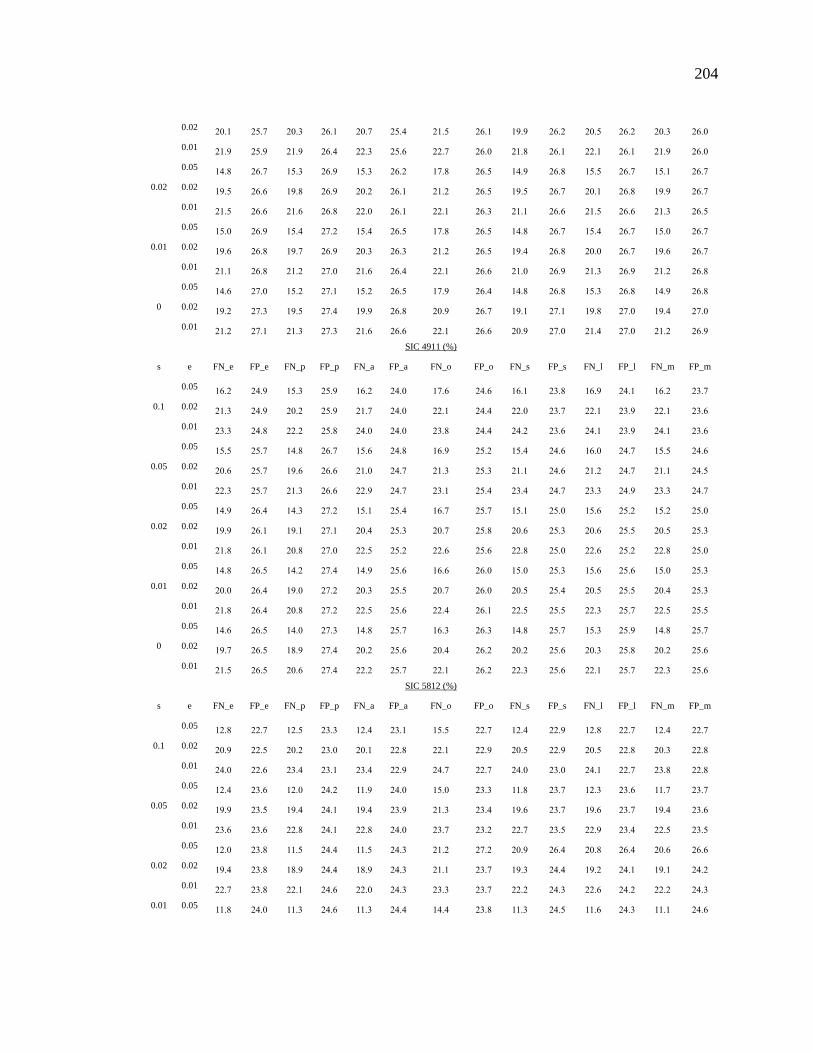
204
0.02 20.1 25.7 20.3 26.1 20.7 25.4 21.5 26.1 19.9 26.2 20.5 26.2 20.3 26.0
0.01 21.9 25.9 21.9 26.4 22.3 25.6 22.7 26.0 21.8 26.1 22.1 26.1 21.9 26.0
0.02
0.05 14.8 26.7 15.3 26.9 15.3 26.2 17.8 26.5 14.9 26.8 15.5 26.7 15.1 26.7
0.02 19.5 26.6 19.8 26.9 20.2 26.1 21.2 26.5 19.5 26.7 20.1 26.8 19.9 26.7
0.01 21.5 26.6 21.6 26.8 22.0 26.1 22.1 26.3 21.1 26.6 21.5 26.6 21.3 26.5
0.01
0.05 15.0 26.9 15.4 27.2 15.4 26.5 17.8 26.5 14.8 26.7 15.4 26.7 15.0 26.7
0.02 19.6 26.8 19.7 26.9 20.3 26.3 21.2 26.5 19.4 26.8 20.0 26.7 19.6 26.7
0.01 21.1 26.8 21.2 27.0 21.6 26.4 22.1 26.6 21.0 26.9 21.3 26.9 21.2 26.8
0
0.05 14.6 27.0 15.2 27.1 15.2 26.5 17.9 26.4 14.8 26.8 15.3 26.8 14.9 26.8
0.02 19.2 27.3 19.5 27.4 19.9 26.8 20.9 26.7 19.1 27.1 19.8 27.0 19.4 27.0
0.01 21.2 27.1 21.3 27.3 21.6 26.6 22.1 26.6 20.9 27.0 21.4 27.0 21.2 26.9
SIC 4911 (%)
s e FN_e FP_e FN_p FP_p FN_a FP_a FN_o FP_o FN_s FP_s FN_l FP_l FN_m FP_m
0.1
0.05 16.2 24.9 15.3 25.9 16.2 24.0 17.6 24.6 16.1 23.8 16.9 24.1 16.2 23.7
0.02 21.3 24.9 20.2 25.9 21.7 24.0 22.1 24.4 22.0 23.7 22.1 23.9 22.1 23.6
0.01 23.3 24.8 22.2 25.8 24.0 24.0 23.8 24.4 24.2 23.6 24.1 23.9 24.1 23.6
0.05
0.05 15.5 25.7 14.8 26.7 15.6 24.8 16.9 25.2 15.4 24.6 16.0 24.7 15.5 24.6
0.02 20.6 25.7 19.6 26.6 21.0 24.7 21.3 25.3 21.1 24.6 21.2 24.7 21.1 24.5
0.01 22.3 25.7 21.3 26.6 22.9 24.7 23.1 25.4 23.4 24.7 23.3 24.9 23.3 24.7
0.02
0.05 14.9 26.4 14.3 27.2 15.1 25.4 16.7 25.7 15.1 25.0 15.6 25.2 15.2 25.0
0.02 19.9 26.1 19.1 27.1 20.4 25.3 20.7 25.8 20.6 25.3 20.6 25.5 20.5 25.3
0.01 21.8 26.1 20.8 27.0 22.5 25.2 22.6 25.6 22.8 25.0 22.6 25.2 22.8 25.0
0.01
0.05 14.8 26.5 14.2 27.4 14.9 25.6 16.6 26.0 15.0 25.3 15.6 25.6 15.0 25.3
0.02 20.0 26.4 19.0 27.2 20.3 25.5 20.7 26.0 20.5 25.4 20.5 25.5 20.4 25.3
0.01 21.8 26.4 20.8 27.2 22.5 25.6 22.4 26.1 22.5 25.5 22.3 25.7 22.5 25.5
0
0.05 14.6 26.5 14.0 27.3 14.8 25.7 16.3 26.3 14.8 25.7 15.3 25.9 14.8 25.7
0.02 19.7 26.5 18.9 27.4 20.2 25.6 20.4 26.2 20.2 25.6 20.3 25.8 20.2 25.6
0.01 21.5 26.5 20.6 27.4 22.2 25.7 22.1 26.2 22.3 25.6 22.1 25.7 22.3 25.6
SIC 5812 (%)
s e FN_e FP_e FN_p FP_p FN_a FP_a FN_o FP_o FN_s FP_s FN_l FP_l FN_m FP_m
0.1
0.05 12.8 22.7 12.5 23.3 12.4 23.1 15.5 22.7 12.4 22.9 12.8 22.7 12.4 22.7
0.02 20.9 22.5 20.2 23.0 20.1 22.8 22.1 22.9 20.5 22.9 20.5 22.8 20.3 22.8
0.01 24.0 22.6 23.4 23.1 23.4 22.9 24.7 22.7 24.0 23.0 24.1 22.7 23.8 22.8
0.05
0.05 12.4 23.6 12.0 24.2 11.9 24.0 15.0 23.3 11.8 23.7 12.3 23.6 11.7 23.7
0.02 19.9 23.5 19.4 24.1 19.4 23.9 21.3 23.4 19.6 23.7 19.6 23.7 19.4 23.6
0.01 23.6 23.6 22.8 24.1 22.8 24.0 23.7 23.2 22.7 23.5 22.9 23.4 22.5 23.5
0.02
0.05 12.0 23.8 11.5 24.4 11.5 24.3 21.2 27.2 20.9 26.4 20.8 26.4 20.6 26.6
0.02 19.4 23.8 18.9 24.4 18.9 24.3 21.1 23.7 19.3 24.4 19.2 24.1 19.1 24.2
0.01 22.7 23.8 22.1 24.6 22.0 24.3 23.3 23.7 22.2 24.3 22.6 24.2 22.2 24.3
0.01 0.05 11.8 24.0 11.3 24.6 11.3 24.4 14.4 23.8 11.3 24.5 11.6 24.3 11.1 24.6

205
0.02 19.3 23.8 18.8 24.5 18.9 24.4 20.7 23.6 19.1 24.4 19.1 24.0 18.8 24.4
0.01 22.5 24.1 21.9 24.8 21.9 24.6 23.5 23.8 22.4 24.4 22.6 24.2 22.2 24.4
0
0.05 11.7 24.3 11.3 24.9 11.3 24.8 14.4 23.9 11.2 24.5 11.5 24.2 11.0 24.5
0.02 19.2 24.3 18.8 25.0 18.8 24.8 20.7 24.1 18.8 24.6 18.8 24.4 18.6 24.7
0.01 22.1 24.0 21.5 24.7 21.5 24.6 23.1 24.0 21.8 24.6 22.1 24.3 21.6 24.6
SIC 7373 (%)
s e FN_e FP_e FN_p FP_p FN_a FP_a FN_o FP_o FN_s FP_s FN_l FP_l FN_m FP_m
0.1
0.05 15.1 24.5 15.4 24.7 15.7 24.2 17.9 25.0 15.5 24.7 15.8 24.7 15.4 24.9
0.02 20.8 24.6 20.9 24.7 21.3 24.4 22.0 25.4 20.9 25.2 21.1 25.0 20.7 25.4
0.01 23.0 24.7 23.0 24.8 23.1 24.3 23.5 25.0 22.9 24.6 23.0 24.5 22.9 24.8
0.05
0.05 14.3 25.6 14.7 25.6 15.3 25.1 17.6 25.5 14.9 25.6 15.3 25.5 14.8 25.8
0.02 19.8 25.7 20.0 25.6 20.4 25.4 21.5 25.6 20.1 25.5 20.6 25.3 19.9 25.7
0.01 22.1 25.9 22.2 25.8 22.5 25.5 23.1 25.9 22.1 25.7 22.3 25.6 22.1 25.9
0.02
0.05 13.5 26.6 13.9 26.5 14.5 26.1 17.3 25.9 14.5 26.1 14.8 25.9 14.5 26.2
0.02 19.0 26.2 19.4 26.2 20.0 25.7 21.2 25.9 19.6 26.1 20.0 25.9 19.5 26.1
0.01 21.7 26.3 21.8 26.2 22.0 25.7 22.7 25.7 21.6 25.9 22.0 25.7 21.6 25.9
0.01
0.05 13.5 26.5 14.0 26.5 14.5 25.9 17.0 26.3 14.2 26.7 14.6 26.5 14.2 26.9
0.02 19.0 26.5 19.5 26.4 20.0 26.0 21.0 26.3 19.3 26.4 19.8 26.3 19.5 26.7
0.01 21.2 26.4 21.5 26.4 21.8 25.9 22.7 25.9 21.6 26.2 22.0 26.1 21.5 26.3
0
0.05 13.2 26.8 13.8 26.6 14.2 26.2 23.3 25.2 21.8 25.9 22.5 25.5 22.0 25.8
0.02 18.5 26.5 19.2 26.1 19.5 25.7 21.7 25.2 19.8 26.0 20.5 25.5 19.9 25.8
0.01 20.8 26.7 21.2 26.4 21.3 26.0 23.4 25.4 21.8 26.1 22.5 25.6 22.0 26.0
SIC 2836 (%)
s e FN_e FP_e FN_p FP_p FN_a FP_a FN_o FP_o FN_s FP_s FN_l FP_l FN_m FP_m
0.1
0.05 19.0 23.0 18.4 23.9 19.4 22.6 22.0 22.1 19.2 22.7 19.5 22.5 19.2 22.5
0.02 23.4 23.0 22.9 23.9 23.7 22.4 24.8 22.1 23.3 22.8 23.5 22.4 23.6 22.4
0.01 25.3 22.8 24.5 23.7 25.7 22.3 26.4 21.9 25.4 22.7 25.8 22.4 25.5 22.3
0.05
0.05 18.7 23.7 17.9 24.7 19.2 23.7 21.3 22.3 18.3 23.2 18.7 23.1 18.3 23.3
0.02 22.7 24.0 22.2 25.0 22.9 23.8 24.3 22.6 22.6 23.5 23.0 23.5 22.5 23.8
0.01 24.1 23.3 23.5 24.3 24.6 23.3 25.9 22.4 25.0 23.4 25.3 23.3 24.9 23.4
0.02
0.05 18.5 23.8 17.9 24.7 18.8 23.5 21.3 23.0 18.1 24.0 18.5 23.9 18.0 24.4
0.02 22.3 24.2 21.6 24.9 22.5 24.0 23.8 23.1 21.6 23.9 22.2 23.7 21.7 24.2
0.01 23.7 23.9 23.3 24.9 24.2 23.7 25.5 22.5 24.4 23.7 24.8 23.6 24.6 24.1
0.01
0.05 18.2 24.3 17.5 24.8 18.7 24.0 21.0 23.0 18.0 24.3 18.4 24.2 18.1 24.4
0.02 22.5 24.5 21.6 25.3 22.7 24.4 24.2 23.1 22.2 24.6 22.7 24.3 22.1 24.6
0.01 23.9 24.5 23.4 25.3 24.3 24.3 25.3 22.8 24.2 24.2 24.5 24.1 24.5 24.5
0
0.05 18.1 24.6 17.4 25.4 18.6 24.4 20.7 23.5 17.4 24.6 17.9 24.4 17.4 24.6
0.02 22.0 25.1 21.0 25.8 22.2 24.6 24.1 23.3 21.8 24.4 22.2 24.2 21.7 24.4
0.01 23.6 24.7 23.1 25.5 24.1 24.5 25.4 22.9 24.0 24.1 24.2 23.9 24.1 24.1
SIC 3845 (%)

206
s e FN_e FP_e FN_p FP_p FN_a FP_a FN_o FP_o FN_s FP_s FN_l FP_l FN_m FP_m
0.1
0.05 16.1 24.2 15.5 24.4 16.5 23.5 19.1 23.6 16.2 23.3 16.3 23.5 16.3 23.8
0.02 21.4 24.2 21.4 24.5 21.9 23.5 23.3 23.6 22.1 23.4 21.9 23.8 21.8 23.9
0.01 23.9 24.0 23.7 24.3 24.6 23.5 24.6 23.6 24.2 23.4 23.8 23.8 23.7 23.9
0.05
0.05 15.3 25.1 14.7 25.2 15.5 24.2 18.4 24.6 15.5 24.6 15.3 25.0 15.5 25.0
0.02 20.6 25.2 20.6 25.4 21.1 24.5 22.7 24.7 21.2 24.8 21.1 25.2 21.0 25.2
0.01 22.7 25.1 22.7 25.2 23.4 24.3 23.9 24.6 23.2 24.7 22.5 25.1 22.5 25.0
0.02
0.05 14.9 25.6 14.4 25.6 15.2 25.0 18.1 25.1 14.8 25.2 14.8 25.9 14.9 25.7
0.02 20.0 25.7 19.9 25.6 20.7 25.2 22.1 24.9 20.7 25.1 20.4 25.7 20.4 25.6
0.01 22.1 25.8 22.2 25.8 22.8 25.3 23.7 24.8 22.7 25.0 22.3 25.6 22.3 25.4
0.01
0.05 14.7 26.0 14.1 25.9 15.0 25.2 17.8 24.8 14.6 25.0 14.5 25.7 14.5 25.5
0.02 20.1 25.8 19.8 25.8 20.5 25.1 21.9 25.2 20.4 25.3 20.2 26.0 20.1 25.8
0.01 22.0 25.7 21.9 25.7 22.7 25.2 23.8 25.1 22.7 25.3 22.4 26.1 22.3 25.9
0
0.05 14.5 26.1 14.1 26.1 14.7 25.4 17.7 24.9 14.5 25.4 14.6 25.9 14.5 25.8
0.02 19.9 26.1 19.7 26.2 20.5 25.4 22.0 25.4 20.3 25.7 20.1 26.2 20.0 26.1
0.01 21.7 26.2 21.6 26.2 22.5 25.6 23.5 25.0 22.5 25.4 22.1 25.9 22.0 25.8
SIC 4813 (%)
s e FN_e FP_e FN_p FP_p FN_a FP_a FN_o FP_o FN_s FP_s FN_l FP_l FN_m FP_m
0.1
0.05 10.4 23.8 10.8 23.7 11.2 23.6 13.7 25.2 10.0 23.8 11.2 23.1 9.7 23.9
0.02 18.7 24.1 19.2 24.1 19.0 23.8 20.4 25.7 18.3 24.1 19.2 23.3 17.8 24.2
0.01 22.0 23.6 22.5 23.7 22.7 23.0 22.4 25.1 22.0 23.6 22.9 22.8 22.0 23.6
0.05
0.05 9.6 24.4 10.2 24.1 10.6 23.9 13.4 26.1 9.5 25.1 10.8 24.4 9.3 25.6
0.02 17.6 24.6 18.2 24.4 18.4 24.4 19.3 25.8 17.7 24.5 18.6 23.9 17.2 25.0
0.01 21.0 24.4 21.3 24.1 21.4 23.9 21.5 26.0 20.7 24.8 21.5 24.1 20.5 25.4
0.02
0.05 9.2 25.6 9.8 25.3 10.3 25.3 13.2 26.7 9.1 25.9 10.4 25.0 8.8 26.0
0.02 17.1 25.4 17.6 25.0 17.5 25.0 19.0 26.0 16.7 25.2 17.7 24.5 16.3 25.4
0.01 20.7 25.4 21.0 25.2 21.2 25.1 21.7 26.1 20.6 25.4 21.4 24.6 20.4 25.7
0.01
0.05 8.8 25.6 9.5 25.3 10.1 25.4 13.3 26.5 9.1 25.6 10.3 25.2 8.8 26.0
0.02 17.0 25.7 17.8 25.4 17.6 25.1 19.0 26.5 16.8 25.8 17.7 25.1 16.4 26.0
0.01 20.4 25.6 20.6 25.3 21.0 25.2 21.3 26.6 20.2 26.1 21.0 25.4 19.9 26.4
0
0.05 9.1 25.9 9.6 25.5 9.9 25.3 12.8 26.5 8.9 26.0 9.9 25.1 8.5 26.1
0.02 16.5 25.6 16.9 25.4 17.2 24.9 18.8 26.9 16.4 26.3 17.4 25.4 15.9 26.4
0.01 19.9 25.9 20.2 25.3 20.2 25.2 21.3 26.1 19.9 25.7 20.8 24.9 19.7 25.9
SIC 3663 (%)
s e FN_e FP_e FN_p FP_p FN_a FP_a FN_o FP_o FN_s FP_s FN_l FP_l FN_m FP_m
0.1
0.05 16.8 25.3 18.1 24.4 17.6 25.1 20.4 23.8 17.7 24.7 17.1 25.3 17.4 25.0
0.02 20.9 25.0 22.3 24.1 21.7 24.8 23.7 23.6 22.0 24.5 21.3 25.1 21.8 24.8
0.01 22.5 25.1 23.8 24.2 23.1 24.8 24.9 24.2 23.7 25.1 23.0 25.9 23.5 25.5
0.05 0.05
16.3 26.5 17.4 25.5 17.0 26.1 19.8 24.8 16.6 25.8 16.2 26.3 16.4 26.0
0.02 20.4 26.3 21.6 25.4 21.1 25.9 23.1 24.6 21.1 25.8 20.5 26.1 21.0 25.9

207
0.01 21.8 26.5 23.0 25.4 22.5 26.0 24.2 24.8 22.7 26.0 22.1 26.4 22.5 26.0
0.02
0.05 16.0 27.2 17.0 26.1 16.6 26.6 19.5 24.8 16.1 26.4 15.8 26.9 15.9 26.5
0.02 19.6 27.1 21.0 26.2 20.3 26.6 22.6 25.0 20.3 26.5 20.0 27.1 20.5 26.6
0.01 21.2 27.5 22.6 26.3 22.1 26.9 23.8 25.0 22.0 26.5 21.5 26.9 21.8 26.3
0.01
0.05 15.8 27.4 16.5 26.1 16.4 26.7 19.7 25.3 16.4 26.9 15.8 27.5 16.1 26.9
0.02 19.1 27.3 20.3 26.3 19.9 26.8 22.3 25.3 20.4 27.0 19.9 27.5 20.5 27.1
0.01 21.2 27.4 22.4 26.2 21.9 26.7 23.5 24.8 21.7 26.4 21.4 26.9 21.5 26.4
0
0.05 15.6 27.2 16.6 26.0 16.2 26.5 19.1 25.1 15.7 26.7 15.2 27.1 15.3 26.6
0.02 19.2 27.5 20.3 26.1 19.8 26.7 22.5 25.1 20.3 26.7 19.8 27.2 20.4 26.8
0.01 20.9 27.7 22.2 26.5 21.8 27.1 23.8 25.2 21.7 26.8 21.2 27.3 21.5 26.7
SIC 4931 (%)
s e FN_e FP_e FN_p FP_p FN_a FP_a FN_o FP_o FN_s FP_s FN_l FP_l FN_m FP_m
0.1
0.05 16.2 24.5 15.1 26.1 16.2 23.5 17.4 24.5 16.0 23.2 17.1 23.2 16.2 23.0
0.02 21.6 24.5 20.3 26.0 21.9 23.4 22.2 24.7 22.2 23.5 22.7 23.5 22.5 23.2
0.01 23.4 24.2 22.0 25.9 24.1 23.4 23.8 24.8 24.1 23.5 24.7 23.5 24.6 23.3
0.05
0.05 15.4 25.3 14.5 26.6 15.7 24.3 16.7 25.3 15.4 24.3 16.2 24.2 15.4 23.9
0.02 20.6 25.4 19.5 26.7 21.4 24.4 21.3 25.4 21.2 24.4 21.5 24.3 21.5 24.1
0.01 22.6 25.3 21.3 26.7 23.3 24.3 23.1 25.2 23.3 24.1 24.0 24.2 23.8 23.8
0.02
0.05 15.1 26.1 14.3 27.4 15.5 25.0 16.2 25.7 14.9 24.8 15.5 24.6 14.9 24.4
0.02 19.9 26.0 19.1 27.3 20.8 25.0 20.7 25.6 20.7 24.8 21.0 24.6 21.0 24.4
0.01 22.2 25.8 21.0 27.0 22.8 24.7 22.5 25.9 22.6 24.9 23.2 24.8 23.1 24.6
0.01
0.05 14.9 26.3 14.0 27.5 15.1 25.1 16.3 26.0 14.7 25.1 15.4 25.0 14.7 24.7
0.02 20.0 26.1 19.1 27.2 20.8 25.0 20.7 25.9 20.6 25.0 21.0 24.8 20.8 24.6
0.01 22.0 25.9 20.8 27.0 22.8 24.9 22.3 26.0 22.3 25.0 22.9 25.0 22.8 24.7
0
0.05 14.8 26.2 14.0 27.4 15.1 25.1 16.4 25.8 14.8 24.9 15.5 24.9 14.9 24.4
0.02 19.9 26.2 19.1 27.4 20.8 25.1 20.7 26.1 20.7 25.2 21.0 25.1 20.9 24.8
0.01 22.0 26.2 20.9 27.4 22.8 25.1 22.2 26.1 22.4 25.3 22.8 25.1 22.7 24.8
SIC 3841 (%)
s e FN_e FP_e FN_p FP_p FN_a FP_a FN_o FP_o FN_s FP_s FN_l FP_l FN_m FP_m
0.1
0.05 11.1 26.1 11.5 25.9 11.6 24.9 14.2 25.9 11.6 24.9 11.6 25.4 11.4 25.2
0.02 18.1 26.3 18.4 26.2 18.4 25.2 19.6 25.7 18.9 25.0 18.3 25.5 18.3 25.4
0.01 20.8 25.8 21.0 25.7 21.4 24.8 22.1 25.1 22.2 24.2 21.1 24.6 22.0 24.6
0.05
0.05 10.8 26.3 11.2 26.4 11.6 25.7 13.3 25.8 11.0 24.9 10.9 25.4 10.8 25.4
0.02 16.9 26.5 17.5 26.4 17.7 25.8 19.0 26.0 18.0 25.4 17.6 25.9 17.7 26.0
0.01 20.4 26.6 20.5 26.5 20.9 26.0 21.1 26.1 20.7 25.3 20.0 26.0 20.5 25.8
0.02
0.05 10.4 27.4 10.7 27.4 10.9 26.5 13.2 26.5 10.6 26.0 10.4 26.9 10.3 26.4
0.02 16.5 26.8 17.1 26.8 17.3 26.1 18.3 26.2 17.2 26.0 17.2 26.6 17.0 26.4
0.01 20.0 27.2 20.1 27.1 20.2 26.3 20.8 26.3 20.6 25.6 19.7 26.5 20.1 26.2
0.01 0.05
10.0 27.3 10.4 27.4 10.5 26.5 13.1 26.2 10.6 26.1 10.6 26.7 10.3 26.4
0.02 16.4 27.1 17.0 27.0 17.0 26.2 18.4 26.2 17.4 25.8 17.2 26.7 17.2 26.3

208
0.01 19.9 27.4 19.9 27.3 20.0 26.4 20.8 26.4 20.8 26.4 19.6 26.9 20.2 26.8
0
0.05 9.9 27.5 10.3 27.5 10.5 26.7 13.1 26.9 10.6 26.3 10.5 27.1 10.3 26.7
0.02 16.1 27.8 16.6 27.5 16.9 26.8 18.2 26.4 17.1 26.2 17.0 27.0 16.9 26.6
0.01 19.6 27.4 19.7 27.4 19.8 26.7 20.2 26.4 20.2 26.3 19.4 26.8 19.7 26.4
SIC 9995 (%)
s e FN_e FP_e FN_p FP_p FN_a FP_a FN_o FP_o FN_s FP_s FN_l FP_l FN_m FP_m
0.1
0.05 23.7 21.9 24.2 22.6 26.8 19.0 28.1 16.4 26.1 17.9 26.8 17.7 27.3 16.6
0.02 26.4 21.7 26.5 22.4 29.1 18.9 31.8 16.9 30.0 18.3 29.1 18.3 29.8 16.9
0.01 26.9 22.1 26.3 21.8 29.2 19.0 31.0 16.8 29.2 18.2 28.7 18.1 29.8 16.8
0.05
0.05 23.6 22.5 23.7 23.5 26.5 19.8 27.9 18.4 24.9 19.9 25.7 20.7 26.4 19.0
0.02 25.2 22.2 24.5 23.0 27.8 18.9 30.4 18.3 28.2 18.9 27.2 20.2 28.9 18.6
0.01 28.2 22.1 27.4 22.9 30.5 19.3 30.7 17.4 29.6 18.9 29.0 19.7 30.9 18.3
0.02
0.05 23.5 22.1 23.0 23.0 26.5 19.3 26.5 18.6 24.0 19.9 25.0 20.8 26.0 19.2
0.02 25.3 23.4 24.6 24.3 27.5 20.0 29.2 17.6 27.9 19.3 26.6 20.0 28.7 18.1
0.01 26.9 22.3 26.6 23.5 29.1 19.6 30.4 18.2 29.0 19.6 28.1 20.9 30.5 18.8
0.01
0.05 23.6 21.9 23.6 22.8 26.8 19.3 28.3 18.5 25.4 20.1 25.8 20.6 27.1 19.0
0.02 25.9 22.3 25.4 23.0 28.5 19.7 29.7 19.0 28.1 20.7 26.7 21.6 28.9 19.6
0.01 26.3 22.8 26.1 23.9 28.2 19.9 30.5 19.1 28.2 20.3 26.9 20.9 29.5 18.6
0
0.05 23.0 23.5 23.0 24.3 25.5 20.2 27.0 17.9 24.1 19.3 25.1 21.0 26.0 18.3
0.02 24.8 23.8 24.6 24.7 27.1 21.0 29.9 18.1 28.1 19.8 27.4 21.2 29.0 18.6
0.01 26.6 23.9 25.9 24.5 28.6 20.8 31.0 18.5 29.1 19.9 27.8 21.0 30.2 18.9
SIC 7990 (%)
s e FN_e FP_e FN_p FP_p FN_a FP_a FN_o FP_o FN_s FP_s FN_l FP_l FN_m FP_m
0.1
0.05 16.7 23.2 16.7 22.8 16.6 23.3 19.0 23.0 16.7 22.9 17.0 22.3 16.6 22.8
0.02 22.3 23.2 23.0 23.2 22.1 23.4 24.0 23.1 22.8 23.0 23.1 22.5 22.3 23.0
0.01 24.2 22.9 24.9 22.8 24.1 23.2 25.0 23.4 24.6 23.4 24.7 22.8 24.3 23.2
0.05
0.05 15.9 23.7 16.0 22.9 15.8 23.9 18.5 23.7 16.1 23.6 16.2 23.4 15.9 23.6
0.02 21.2 24.2 21.8 23.7 20.5 24.5 23.1 23.9 21.6 23.8 21.7 23.7 21.1 23.9
0.01 23.3 24.6 23.8 23.9 23.0 24.9 24.6 24.0 23.9 24.2 24.3 24.1 23.7 24.2
0.02
0.05 15.5 24.7 15.6 24.4 15.5 25.2 18.4 25.2 15.9 25.4 16.1 25.0 15.7 25.3
0.02 20.7 25.0 21.2 24.5 20.2 25.5 22.3 24.6 20.8 24.7 21.0 24.4 20.6 24.7
0.01 22.9 24.9 23.4 24.5 22.8 25.5 24.1 24.3 23.2 24.5 23.7 24.2 23.0 24.4
0.01
0.05 15.5 24.7 15.7 24.2 15.6 25.2 18.1 24.8 15.5 24.8 15.5 24.6 15.2 24.9
0.02 21.0 24.6 21.7 24.3 20.5 25.1 22.3 24.4 21.0 24.8 21.2 24.4 20.6 24.8
0.01 22.9 24.8 23.6 24.5 22.5 25.1 24.2 24.5 23.1 24.6 23.6 24.4 22.8 24.7
0
0.05 15.0 25.1 15.2 24.8 15.1 25.7 17.8 24.5 15.2 24.6 15.2 24.3 14.9 24.7
0.02 20.4 25.5 20.9 25.0 19.7 25.8 22.2 24.8 20.5 24.9 20.9 24.4 20.3 25.0
0.01 22.7 25.2 23.3 24.9 22.2 25.7 23.8 25.0 22.6 25.0 22.9 24.6 22.3 25.1
SIC 3714 (%)
s e FN_e FP_e FN_p FP_p FN_a FP_a FN_o FP_o FN_s FP_s FN_l FP_l FN_m FP_m

209
0.1
0.05 15.8 22.8 15.9 23.1 14.9 23.4 17.1 23.5 15.1 22.2 15.5 22.6 15.2 22.4
0.02 22.3 22.6 22.3 23.1 21.4 23.3 22.1 23.9 22.0 22.7 22.1 23.1 21.8 23.1
0.01 24.7 22.6 24.8 23.1 23.8 23.3 24.1 23.9 24.5 22.4 24.7 22.7 24.4 22.7
0.05
0.05 15.2 23.9 15.1 24.1 14.3 24.5 16.7 24.9 14.4 23.9 14.8 24.0 14.4 23.9
0.02 21.8 23.4 21.4 23.8 20.6 24.3 21.6 24.6 21.1 23.5 21.0 23.6 20.8 23.6
0.01 24.1 23.8 24.3 24.1 23.1 24.6 23.0 24.9 23.8 23.9 23.5 24.2 23.5 24.1
0.02
0.05 14.3 24.2 14.3 24.1 13.6 24.7 21.0 24.9 20.2 23.8 20.4 24.2 20.2 24.1
0.02 21.3 24.4 20.8 24.3 20.0 25.3 21.0 24.9 20.2 23.8 20.4 24.2 20.2 24.1
0.01 22.9 24.1 23.1 24.2 21.8 24.9 23.1 24.9 23.5 24.1 23.4 24.4 23.6 24.2
0.01
0.05 14.5 24.3 14.4 24.3 13.7 24.8 16.3 25.4 14.0 24.5 14.3 24.7 14.0 24.6
0.02 20.8 24.5 20.5 24.4 19.4 25.1 21.3 24.8 20.7 24.0 20.8 24.3 20.4 24.0
0.01 23.0 24.3 23.2 24.4 22.0 25.0 22.9 25.6 23.0 24.7 23.0 24.9 23.1 24.7
0
0.05 14.3 24.8 14.4 24.7 13.5 25.4 16.5 25.5 14.1 24.6 14.5 24.7 14.2 24.6
0.02 20.5 25.1 20.2 25.0 19.1 25.6 21.1 25.7 20.4 24.9 20.6 25.0 20.2 24.9
0.01 23.0 24.6 23.0 24.5 22.0 25.2 22.8 25.8 22.7 24.8 22.9 25.0 23.0 24.8
SIC 6331 (%)
s e FN_e FP_e FN_p FP_p FN_a FP_a FN_o FP_o FN_s FP_s FN_l FP_l FN_m FP_m
0.1
0.05 13.1 24.6 13.1 24.8 13.1 24.1 14.8 25.9 12.9 24.9 13.3 24.9 13.3 25.3
0.02 18.9 24.7 19.3 24.9 19.4 24.5 20.0 25.7 19.6 24.8 19.3 24.7 19.4 25.1
0.01 21.7 25.1 21.9 25.3 22.1 24.6 22.2 25.7 22.1 24.8 22.2 24.8 22.0 25.2
0.05
0.05 12.2 26.2 12.5 26.3 12.5 25.6 14.2 26.3 12.5 26.1 12.7 25.6 12.5 26.1
0.02 18.1 25.9 18.3 25.8 18.7 25.3 19.5 26.4 18.5 25.8 18.7 25.6 18.8 26.1
0.01 20.9 26.4 21.2 26.6 21.4 25.7 21.4 26.5 21.4 25.9 21.3 25.6 21.3 26.1
0.02
0.05 11.6 26.4 11.9 26.4 11.8 26.0 25.2 22.7 24.5 22.8 24.4 23.0 24.5 22.9
0.02 18.1 26.7 18.2 26.6 18.5 26.0 18.9 27.2 17.9 26.5 18.1 26.7 17.8 26.7
0.01 20.4 26.9 20.5 27.1 20.7 26.3 21.2 27.2 20.9 26.4 20.8 26.4 20.6 26.6
0.01
0.05 11.8 27.0 11.9 27.0 11.8 26.4 13.5 26.8 11.6 26.3 11.9 26.3 11.7 26.6
0.02 18.2 27.0 18.6 27.2 18.7 26.4 18.8 27.1 17.9 26.7 18.1 26.9 17.7 27.0
0.01 20.6 26.6 20.6 26.8 20.9 26.1 20.7 26.7 20.8 26.4 20.4 26.4 20.5 26.7
0
0.05 11.6 26.8 11.9 27.0 11.8 26.3 13.8 27.4 11.7 26.9 12.0 26.9 11.8 27.2
0.02 17.6 27.2 17.7 27.1 18.1 26.6 18.7 27.7 17.3 27.2 17.7 27.0 17.2 27.4
0.01 20.0 27.1 20.3 27.3 20.5 26.5 21.0 27.6 20.7 26.9 20.5 26.9 20.4 27.2
SIC 6211 (%)
s e FN_e FP_e FN_p FP_p FN_a FP_a FN_o FP_o FN_s FP_s FN_l FP_l FN_m FP_m
0.1
0.05 18.0 24.5 17.2 24.5 18.0 24.5 20.7 23.3 18.5 24.4 18.9 22.1 18.6 22.8
0.02 22.8 24.3 22.0 24.5 22.5 24.2 24.0 23.6 22.2 24.6 24.3 22.8 23.7 23.3
0.01 24.1 23.7 23.8 24.3 24.0 23.9 25.2 23.0 24.2 24.2 25.6 22.0 25.3 22.6
0.05
0.05 17.4 25.5 16.5 25.8 16.9 24.9 19.8 24.7 17.7 25.7 18.6 24.1 18.2 24.5
0.02 22.0 24.6 21.1 25.2 21.6 24.4 23.8 24.6 22.1 25.3 22.6 23.6 23.0 24.0
0.01 23.7 24.7 22.5 25.3 23.4 24.5 24.1 24.3 23.1 25.5 24.3 23.8 24.2 24.2

210
0.02
0.05 16.8 25.4 16.4 26.8 17.1 25.6 24.1 24.2 22.7 25.3 23.7 23.9 23.8 24.3
0.02 22.3 25.1 21.3 26.0 21.5 24.9 22.9 24.9 21.5 26.0 22.5 24.7 22.3 25.0
0.01 23.0 26.1 22.2 27.0 23.0 26.0 24.2 24.7 22.9 25.7 23.9 24.0 23.8 24.5
0.01
0.05 16.2 25.2 16.0 26.3 16.3 25.1 19.2 25.2 17.1 26.2 17.7 25.0 17.7 25.3
0.02 20.9 25.4 20.5 26.8 20.6 25.4 23.0 25.0 21.7 25.8 21.6 24.4 21.9 24.6
0.01 23.5 25.2 22.3 26.1 23.1 24.9 23.7 24.9 22.5 26.1 23.4 24.5 23.5 25.0
0
0.05 16.4 25.9 16.0 26.6 16.3 25.6 19.5 24.7 17.1 25.7 17.8 24.2 17.9 24.7
0.02 21.3 25.8 20.4 26.6 20.9 25.7 23.3 25.7 21.6 26.2 21.9 24.8 22.0 25.3
0.01 22.0 25.3 21.4 26.7 22.0 25.2 23.7 26.1 22.3 26.9 23.4 25.8 22.9 25.9
SIC 3576 (%)
s e FN_e FP_e FN_p FP_p FN_a FP_a FN_o FP_o FN_s FP_s FN_l FP_l FN_m FP_m
0.1
0.05 21.3 20.6 24.1 18.5 22.0 19.1 25.1 18.5 22.9 19.9 22.7 19.9 22.7 20.2
0.02 26.5 20.4 28.8 18.4 27.0 19.3 29.7 18.2 27.7 19.1 28.2 19.5 26.9 19.4
0.01 27.7 21.6 30.0 19.5 28.9 20.3 31.3 19.1 30.0 20.1 29.8 20.0 29.5 20.2
0.05
0.05 19.8 21.5 22.5 19.3 20.5 20.2 23.7 19.1 21.5 20.4 21.1 20.8 21.2 21.0
0.02 25.7 21.5 27.8 19.1 26.5 20.3 29.1 19.1 27.1 20.6 27.5 20.9 27.1 21.0
0.01 26.3 22.0 28.7 19.5 27.7 20.6 29.8 19.1 28.2 19.7 28.3 20.4 27.5 20.8
0.02
0.05 20.0 21.6 22.8 19.4 20.5 20.6 23.6 19.3 20.7 20.3 20.8 21.0 20.5 20.9
0.02 25.1 23.0 27.9 20.5 25.7 21.7 28.4 20.0 26.5 21.5 25.9 21.9 26.0 22.2
0.01 27.1 21.4 29.8 18.8 28.0 20.3 30.3 18.8 28.3 19.8 28.9 20.3 27.9 20.4
0.01
0.05 19.3 22.8 22.0 20.0 20.4 21.8 23.3 19.2 20.8 20.7 20.6 20.8 20.8 21.4
0.02 24.6 22.2 27.5 19.7 25.4 21.2 28.4 19.6 26.3 21.4 26.1 21.5 25.7 22.0
0.01 25.2 21.8 27.9 19.0 26.5 20.9 29.7 18.8 27.5 20.3 28.5 20.6 27.4 20.8
0
0.05 19.8 23.0 22.0 20.1 20.6 21.9 23.6 19.4 20.8 21.5 21.0 21.5 21.1 22.0
0.02 23.9 22.7 27.1 20.5 25.1 21.7 28.2 20.0 25.7 21.5 24.9 21.3 24.8 21.9
0.01 26.2 22.5 28.6 19.7 27.1 21.3 29.8 19.0 27.8 20.8 28.8 21.2 27.7 21.6
Panel B. The Error Detection Performance in Cost of Goods Sold Account
SIC 7372 (%) s e FN_e FP_e FN_p FP_p FN_a FP_a FN_o FP_o FN_s FP_s FN_l FP_l FN_m FP_m
0.1
0.05 21.6 22.2 21.6 22.1 21.7 22.1 20.8 25.0 17.9 25.9 18.5 25.6 17.8 25.8
0.02 25.5 21.9 25.5 21.8 25.6 21.9 23.4 25.0 21.9 25.8 22.0 25.6 21.8 25.8
0.01 26.5 22.2 26.6 22.1 26.6 22.1 24.2 25.1 23.0 25.9 23.2 25.6 23.0 25.8
0.05
0.05 20.8 23.2 20.6 23.0 20.6 23.0 21.4 24.5 18.8 24.9 19.3 24.7 18.8 24.8
0.02 24.4 23.1 24.5 23.0 24.6 22.9 23.9 24.4 22.6 24.8 22.9 24.7 22.8 24.8
0.01 25.7 23.0 25.7 22.8 25.7 22.9 24.8 24.4 23.9 24.8 24.1 24.6 23.9 24.7
0.02
0.05 20.3 23.5 20.1 23.6 20.2 23.5 22.0 24.0 19.6 24.1 20.1 24.1 19.6 24.0
0.02 24.0 23.5 23.9 23.6 24.1 23.6 24.2 24.1 23.2 24.2 23.3 24.2 23.3 24.1
0.01 25.0 23.5 25.0 23.5 25.1 23.5 25.1 24.0 24.5 24.1 24.6 24.0 24.5 24.0
0.01 0.05
20.1 23.7 20.0 23.7 20.0 23.7 22.0 23.9 19.7 24.0 20.0 23.9 19.6 24.0
0.02 23.9 23.9 23.7 23.9 23.9 23.9 24.1 24.0 23.2 24.0 23.3 23.9 23.4 24.0

211
0.01 24.9 23.9 25.0 23.9 25.1 23.8 25.2 24.1 24.7 24.2 24.8 24.1 24.7 24.0
0
0.05 19.8 23.7 19.9 23.9 19.8 23.9 22.0 23.9 19.7 23.9 20.1 23.9 19.8 23.8
0.02 23.1 23.9 23.5 23.6 23.6 23.7 24.5 23.8 23.6 23.9 23.7 23.7 23.6 23.7
0.01 24.8 23.9 23.9 23.5 24.5 24.0 25.4 23.8 25.0 23.8 25.0 23.7 25.0 23.6
SIC 1311 (%)
s e FN_e FP_e FN_p FP_p FN_a FP_a FN_o FP_o FN_s FP_s FN_l FP_l FN_m FP_m
0.1
0.05 18.9 22.9 20.0 22.1 19.7 22.0 19.9 27.2 18.8 27.1 19.3 26.5 19.3 26.4
0.02 22.9 22.8 24.1 22.2 23.8 22.0 21.7 27.3 21.2 27.2 21.7 26.6 21.7 26.5
0.01 25.6 22.7 26.5 22.0 26.5 21.8 22.4 27.1 22.1 27.0 22.7 26.4 22.7 26.3
0.05
0.05 18.0 23.8 19.1 23.0 18.9 22.9 20.8 26.5 20.1 26.2 20.7 25.5 20.6 25.6
0.02 21.9 24.1 23.1 23.2 22.8 23.1 22.4 26.5 22.1 26.0 22.9 25.4 22.9 25.5
0.01 24.3 24.0 25.3 23.1 25.2 22.9 23.2 26.5 23.3 26.1 24.0 25.5 24.1 25.5
0.02
0.05 17.2 24.8 18.2 23.8 18.0 23.8 21.1 26.1 20.6 25.4 21.2 24.6 21.0 24.8
0.02 21.2 24.6 22.3 23.6 22.2 23.7 22.9 26.3 22.9 25.5 23.7 24.7 23.5 24.9
0.01 23.7 24.8 24.6 23.7 24.6 23.7 23.3 26.1 23.9 25.5 24.7 24.8 24.5 25.0
0.01
0.05 17.1 24.8 18.2 23.8 18.0 23.8 21.1 26.0 20.8 25.3 21.4 24.4 21.2 24.7
0.02 21.0 24.9 22.0 23.8 21.9 24.0 22.9 26.0 23.3 25.3 23.9 24.3 23.9 24.7
0.01 23.4 24.7 24.4 23.8 24.4 23.8 23.4 25.9 24.0 25.3 24.8 24.5 24.7 24.8
0
0.05 16.8 25.2 17.7 24.3 17.6 24.3 21.3 25.7 21.0 24.7 21.7 23.9 21.6 24.2
0.02 20.7 25.1 21.8 24.2 21.6 24.2 23.1 25.8 23.6 24.9 24.3 24.1 24.2 24.4
0.01 23.3 25.2 24.2 24.2 24.2 24.3 23.6 25.8 24.1 24.8 25.1 24.1 24.8 24.4
SIC 7370 (%)
s e FN_e FP_e FN_p FP_p FN_a FP_a FN_o FP_o FN_s FP_s FN_l FP_l FN_m FP_m
0.1
0.05 18.3 23.2 18.2 23.4 18.1 23.6 17.9 26.7 15.2 26.6 15.1 26.3 15.4 25.8
0.02 23.3 23.0 23.5 23.2 23.4 23.4 21.1 27.1 19.8 27.0 19.9 26.7 20.1 26.1
0.01 25.4 23.2 25.2 23.3 25.1 23.5 22.1 26.7 21.4 26.5 21.5 26.3 22.1 25.7
0.05
0.05 17.5 24.1 17.4 24.2 17.2 24.3 18.6 26.2 16.2 25.8 16.0 25.6 16.4 24.9
0.02 22.8 24.1 22.8 24.2 22.8 24.3 21.6 26.4 20.8 26.0 20.9 26.0 21.2 25.2
0.01 24.2 24.0 24.3 24.1 24.0 24.1 22.7 26.4 22.6 26.0 22.6 25.8 23.3 25.1
0.02
0.05 17.2 24.4 16.9 24.4 16.7 24.6 18.8 26.2 16.5 25.5 16.4 25.5 16.7 24.8
0.02 22.1 24.3 22.1 24.4 22.1 24.7 21.8 26.2 21.1 25.5 21.4 25.4 21.7 24.8
0.01 23.6 24.6 23.6 24.7 23.8 25.0 23.0 26.0 23.1 25.3 23.2 25.3 23.7 24.5
0.01
0.05 17.0 24.6 16.8 24.6 16.5 24.9 18.9 26.2 16.8 25.3 16.6 25.5 16.8 24.6
0.02 22.0 24.6 22.0 24.8 21.8 25.0 22.1 26.1 21.4 25.2 21.7 25.2 22.1 24.5
0.01 23.6 24.4 23.4 24.3 23.6 24.6 23.2 26.1 23.4 25.3 23.3 25.2 24.0 24.5
0
0.05 16.7 24.8 16.7 24.9 16.2 25.0 19.1 25.7 17.0 24.8 16.8 24.7 17.1 24.0
0.02 21.6 24.9 21.5 25.1 21.3 25.2 22.2 25.7 21.4 24.6 21.9 24.7 22.1 23.9
0.01 23.5 24.9 23.3 25.0 23.5 25.2 23.4 25.7 23.6 24.8 23.8 24.9 24.4 24.1
SIC 2834 (%)
s e FN_e FP_e FN_p FP_p FN_a FP_a FN_o FP_o FN_s FP_s FN_l FP_l FN_m FP_m

212
0.1
0.05 21.6 22.1 21.8 21.9 21.5 22.1 19.2 26.5 17.9 26.4 17.7 26.4 17.8 26.2
0.02 25.6 22.0 26.1 21.8 25.5 21.9 22.3 26.2 21.6 26.1 21.7 26.2 21.7 25.8
0.01 26.6 21.9 27.0 21.8 26.7 21.8 22.9 26.4 22.5 26.3 22.7 26.4 22.7 26.1
0.05
0.05 20.6 23.1 20.8 22.9 20.5 23.1 19.9 25.8 18.6 25.4 18.6 25.4 18.7 25.1
0.02 24.4 23.2 24.8 23.0 24.2 23.0 22.8 25.9 22.2 25.3 22.4 25.3 22.4 25.1
0.01 25.8 23.5 26.3 23.3 25.7 23.3 23.5 26.0 23.4 25.6 23.6 25.5 23.8 25.3
0.02
0.05 19.7 23.8 20.1 23.5 19.6 23.8 20.2 25.4 19.1 24.9 19.1 24.9 19.3 24.7
0.02 24.0 23.7 24.5 23.5 23.9 23.7 22.9 25.5 22.5 24.8 22.9 24.9 22.7 24.6
0.01 25.2 23.6 25.6 23.3 25.2 23.6 23.8 25.4 24.0 24.8 24.1 24.7 24.3 24.6
0.01
0.05 19.9 23.8 20.0 23.4 19.7 23.8 20.3 25.1 19.2 24.6 19.1 24.5 19.3 24.4
0.02 23.8 23.4 24.3 23.2 23.5 23.4 23.1 25.1 22.9 24.6 23.1 24.4 23.0 24.4
0.01 25.0 23.5 25.4 23.3 24.9 23.5 24.0 25.3 24.1 24.4 24.3 24.4 24.2 24.2
0
0.05 19.7 23.6 19.9 23.5 19.6 23.8 20.3 25.4 19.2 24.7 19.3 24.6 19.3 24.7
0.02 23.8 23.8 24.0 23.7 23.6 24.0 23.1 25.2 22.8 24.6 23.2 24.6 23.1 24.5
0.01 24.5 23.6 25.1 23.6 24.5 23.8 24.0 25.3 24.2 24.5 24.3 24.3 24.4 24.4
SIC 3674 (%)
s e FN_e FP_e FN_p FP_p FN_a FP_a FN_o FP_o FN_s FP_s FN_l FP_l FN_m FP_m
0.1
0.05 20.3 22.2 21.3 21.2 20.7 21.5 19.4 25.3 17.2 25.5 17.3 25.5 17.4 25.4
0.02 24.6 22.3 25.8 21.1 25.4 21.5 22.5 25.5 21.5 25.7 21.6 25.7 21.7 25.5
0.01 26.4 22.4 27.5 21.3 27.0 21.7 23.7 25.3 23.2 25.4 23.0 25.5 23.2 25.2
0.05
0.05 19.7 23.1 20.6 22.0 20.1 22.4 20.0 24.8 18.0 24.8 18.1 24.8 18.2 24.7
0.02 23.9 23.2 25.0 22.1 24.3 22.5 23.1 24.6 22.5 24.7 22.4 24.6 22.6 24.6
0.01 25.4 23.1 26.5 21.9 26.1 22.4 24.2 24.5 23.9 24.5 23.8 24.5 24.1 24.4
0.02
0.05 19.0 23.8 20.0 22.6 19.4 22.9 20.5 24.4 18.6 24.1 19.0 24.1 18.9 24.1
0.02 23.5 23.5 24.5 22.3 24.0 22.7 23.4 24.4 22.9 24.1 22.8 24.2 23.0 24.1
0.01 25.0 23.6 25.9 22.4 25.6 22.7 24.4 24.6 24.1 24.2 24.0 24.3 24.3 24.1
0.01
0.05 18.8 23.6 19.8 22.7 19.3 23.0 20.4 24.3 18.7 24.1 19.0 24.1 19.0 24.0
0.02 23.3 23.7 24.3 22.7 23.9 23.1 23.5 24.2 23.1 24.0 23.0 24.0 23.2 23.9
0.01 24.9 23.7 25.9 22.7 25.6 23.0 24.9 24.2 24.8 23.9 24.7 23.9 24.9 23.8
0
0.05 18.9 23.9 19.6 22.9 19.2 23.1 20.6 24.0 18.8 23.7 19.1 23.7 19.0 23.7
0.02 23.1 23.8 24.1 22.9 23.4 23.1 23.7 24.1 23.2 23.6 23.1 23.7 23.3 23.5
0.01 24.4 23.8 25.3 22.7 25.0 23.1 24.7 23.9 24.6 23.4 24.6 23.5 24.7 23.4
SIC 4911 (%)
s e FN_e FP_e FN_p FP_p FN_a FP_a FN_o FP_o FN_s FP_s FN_l FP_l FN_m FP_m
0.1
0.05 19.0 22.6 20.5 21.5 20.1 20.9 17.8 25.5 15.5 25.9 16.4 25.7 16.0 25.8
0.02 23.9 22.7 25.1 21.6 25.4 20.9 22.0 25.4 20.5 25.6 21.2 25.5 20.8 25.5
0.01 25.6 22.6 26.6 21.4 27.2 20.7 23.1 25.6 22.2 26.0 22.8 25.8 22.5 25.8
0.05
0.05 18.2 23.4 19.7 22.5 19.3 21.7 18.4 24.9 16.3 25.1 17.2 24.8 16.6 25.0
0.02 23.2 23.7 24.5 22.7 24.5 21.9 22.3 24.8 21.1 24.9 21.8 24.7 21.4 24.8
0.01 24.8 23.5 25.7 22.6 26.4 21.7 23.8 25.0 23.1 25.1 23.7 24.9 23.3 25.0

213
0.02
0.05 17.5 24.0 18.9 23.1 18.8 22.2 19.1 24.4 16.9 24.4 17.9 24.2 17.2 24.3
0.02 22.4 23.9 23.7 23.0 23.9 22.3 23.0 24.6 21.9 24.6 22.6 24.3 22.2 24.5
0.01 24.3 24.0 25.3 23.1 25.7 22.3 24.3 24.4 23.8 24.5 24.2 24.1 23.9 24.4
0.01
0.05 17.2 24.1 18.7 23.2 18.6 22.5 19.3 24.3 17.0 24.2 18.1 24.0 17.3 24.1
0.02 22.4 24.4 23.5 23.3 23.8 22.5 23.2 24.3 22.2 24.3 22.9 24.1 22.5 24.3
0.01 24.1 24.3 25.1 23.4 25.5 22.6 24.4 24.3 23.8 24.2 24.3 24.0 23.9 24.2
0
0.05 17.2 24.3 18.6 23.4 18.4 22.6 19.3 24.1 17.2 24.2 18.2 23.8 17.5 24.0
0.02 22.2 24.3 23.4 23.5 23.7 22.6 23.3 24.2 22.4 24.2 23.0 23.9 22.6 24.1
0.01 24.1 24.3 25.1 23.3 25.4 22.5 24.6 24.1 24.2 24.0 24.6 23.7 24.3 24.0
SIC 5812 (%)
s e FN_e FP_e FN_p FP_p FN_a FP_a FN_o FP_o FN_s FP_s FN_l FP_l FN_m FP_m
0.1
0.05 11.2 24.8 11.5 24.7 11.6 24.2 13.3 26.0 10.4 26.2 10.1 26.7 10.4 26.0
0.02 18.5 25.0 18.9 24.8 19.4 24.2 19.5 26.1 17.4 26.3 17.2 26.8 17.5 26.1
0.01 21.7 25.2 22.2 24.9 22.6 24.4 21.7 26.1 20.4 26.2 20.4 26.8 20.6 26.0
0.05
0.05 11.7 24.2 12.0 23.9 12.2 23.3 13.9 25.3 11.1 25.3 10.8 25.8 11.1 25.2
0.02 19.3 24.1 19.7 23.8 20.2 23.2 20.1 25.2 18.4 25.2 18.1 25.7 18.5 25.1
0.01 22.5 24.2 22.9 24.0 23.5 23.3 22.3 25.2 21.4 25.3 21.3 25.7 21.6 25.2
0.02
0.05 11.2 24.6 11.6 24.6 11.8 24.1 14.1 25.0 11.4 24.7 11.1 25.2 11.3 24.6
0.02 18.7 24.5 19.1 24.3 19.7 23.8 20.2 24.9 18.8 24.9 18.5 25.3 18.8 24.7
0.01 22.2 24.4 22.9 24.4 23.1 23.7 22.6 24.6 21.7 24.5 21.6 24.8 21.8 24.3
0.01
0.05 11.3 24.8 11.6 24.5 11.8 24.0 14.2 24.7 11.5 24.5 11.2 25.0 11.4 24.4
0.02 18.5 24.8 18.9 24.6 19.4 24.0 20.5 24.9 18.9 24.6 18.6 24.9 18.9 24.3
0.01 22.0 24.4 22.6 24.3 23.0 23.8 23.1 24.8 22.3 24.7 22.2 25.0 22.4 24.5
0
0.05 11.0 25.1 11.3 24.9 11.3 24.4 14.4 24.6 11.7 24.5 11.2 24.7 11.6 24.3
0.02 18.6 24.8 18.9 24.5 19.5 23.9 20.4 24.6 19.1 24.4 18.9 24.9 19.1 24.4
0.01 21.5 25.2 22.1 25.0 22.5 24.3 22.8 24.8 22.0 24.6 21.8 24.9 22.1 24.4
SIC 7373 (%)
s e FN_e FP_e FN_p FP_p FN_a FP_a FN_o FP_o FN_s FP_s FN_l FP_l FN_m FP_m
0.1
0.05 17.3 23.5 17.1 23.1 17.1 23.4 18.0 25.4 16.1 25.3 15.5 25.9 15.8 25.5
0.02 22.8 23.7 22.9 23.4 23.0 23.7 21.8 25.7 20.9 25.3 20.3 26.3 20.7 25.6
0.01 24.4 23.8 24.9 23.4 24.8 23.6 23.2 25.7 22.6 25.4 22.2 26.3 22.6 25.7
0.05
0.05 17.8 23.7 17.7 23.4 17.7 23.9 18.5 25.0 16.8 24.5 15.9 25.1 16.4 24.8
0.02 23.1 23.4 23.2 23.1 23.3 23.5 22.6 25.2 21.8 24.8 21.4 25.4 21.8 24.9
0.01 24.4 23.8 24.8 23.5 24.8 23.9 24.0 25.0 23.6 24.5 23.1 25.0 23.4 24.6
0.02
0.05 17.8 23.3 17.6 23.0 17.5 23.4 18.9 25.0 17.0 24.3 16.4 24.4 16.7 24.4
0.02 23.3 23.4 23.5 23.3 23.4 23.6 22.9 25.0 22.1 24.4 21.7 24.6 22.1 24.5
0.01 24.5 23.2 25.0 23.0 24.8 23.4 24.4 24.6 24.3 24.1 23.9 24.4 24.2 24.2
0.01
0.05 18.4 22.9 18.2 22.5 18.5 23.1 19.2 24.6 17.6 23.7 16.9 24.0 17.2 23.8
0.02 23.6 22.7 23.7 22.5 23.7 22.9 23.0 24.4 22.2 23.7 21.9 24.0 22.1 23.7
0.01 25.4 23.1 26.0 22.7 25.5 23.1 24.2 24.4 24.1 23.7 23.6 23.9 24.1 23.8

214
0
0.05 19.0 21.8 19.2 21.7 19.2 21.7 19.5 24.2 17.9 23.5 17.1 23.7 17.4 23.5
0.02 24.3 22.1 24.9 22.0 24.4 22.1 23.4 23.9 22.7 23.3 22.5 23.5 22.7 23.4
0.01 26.1 22.0 26.8 21.8 26.3 22.0 24.3 24.3 24.3 23.7 23.9 23.7 24.3 23.7
SIC 2836 (%)
s e FN_e FP_e FN_p FP_p FN_a FP_a FN_o FP_o FN_s FP_s FN_l FP_l FN_m FP_m
0.1
0.05 22.5 21.4 23.0 20.7 22.6 21.0 21.3 24.9 19.3 24.7 19.2 25.1 19.0 24.6
0.02 26.2 21.3 26.5 20.8 26.7 21.1 23.6 25.1 22.8 25.0 22.5 25.1 22.7 24.8
0.01 27.2 21.6 27.5 21.0 27.4 21.1 24.9 24.4 24.7 24.8 24.4 24.9 24.7 24.4
0.05
0.05 21.8 22.6 22.0 22.0 21.6 22.0 22.0 24.2 20.4 23.8 20.2 23.8 20.1 23.9
0.02 25.1 22.5 25.6 22.1 25.6 22.0 24.5 23.5 24.0 23.4 23.8 23.2 23.8 23.4
0.01 26.7 22.4 27.1 22.1 27.1 21.7 25.4 24.0 25.1 23.6 25.2 23.6 25.1 23.7
0.02
0.05 21.8 22.7 21.6 22.1 21.7 22.3 22.3 23.6 20.8 23.2 20.7 23.4 20.7 23.3
0.02 24.7 23.0 24.9 22.3 25.1 22.4 24.9 23.4 24.7 23.3 24.6 23.8 24.7 23.6
0.01 25.5 23.1 25.9 22.3 26.0 22.5 25.6 23.2 25.7 23.1 25.8 23.2 25.8 23.4
0.01
0.05 21.2 22.9 21.1 22.6 21.1 22.4 22.1 23.1 20.8 22.9 20.9 23.1 20.6 23.2
0.02 25.0 23.1 25.3 22.7 25.4 22.6 24.6 23.2 24.4 23.1 24.1 23.2 24.3 23.2
0.01 25.7 23.0 26.0 22.4 26.4 22.5 25.8 23.3 25.9 23.0 25.9 23.2 26.0 23.3
0
0.05 20.8 23.0 20.8 22.4 20.7 22.4 22.4 23.4 20.9 23.0 21.0 23.2 20.9 23.3
0.02 24.7 23.5 24.7 22.9 24.7 22.8 25.2 23.0 25.1 22.9 24.8 22.9 24.9 23.0
0.01 26.0 23.6 26.2 23.0 26.1 22.8 25.7 23.3 25.6 22.9 25.7 23.2 25.8 23.3
SIC 3845 (%)
s e FN_e FP_e FN_p FP_p FN_a FP_a FN_o FP_o FN_s FP_s FN_l FP_l FN_m FP_m
0.1
0.05 20.8 22.1 21.5 20.9 21.4 21.2 19.3 24.8 17.3 25.1 17.9 24.7 17.6 24.8
0.02 25.3 22.2 26.2 21.0 26.1 21.3 22.9 24.8 21.9 25.1 22.5 24.6 22.5 24.8
0.01 26.6 21.9 27.8 20.8 27.4 21.1 24.3 24.9 23.4 25.0 24.0 24.6 24.0 24.7
0.05
0.05 19.9 23.0 20.4 21.7 20.3 22.3 20.1 24.1 18.5 23.9 18.9 23.5 18.7 23.6
0.02 24.1 22.9 25.0 21.6 24.9 22.2 23.4 24.5 22.7 24.5 23.2 23.9 23.4 24.2
0.01 25.8 23.0 26.8 21.8 26.4 22.2 24.2 24.2 23.9 24.2 24.5 23.8 24.4 23.9
0.02
0.05 19.6 23.7 20.1 22.5 19.8 22.9 20.4 24.0 18.9 23.8 19.2 23.5 19.0 23.5
0.02 23.6 23.4 24.5 22.3 24.3 22.7 23.7 23.8 23.3 23.7 23.7 23.4 23.8 23.4
0.01 25.0 23.5 25.9 22.3 25.7 22.8 25.1 24.1 24.9 23.8 25.3 23.6 25.2 23.6
0.01
0.05 19.4 23.5 19.7 22.5 19.6 22.9 20.4 23.9 18.9 23.6 19.2 23.3 19.1 23.3
0.02 23.5 23.7 24.2 22.5 24.0 22.9 23.7 23.7 23.3 23.4 23.7 23.2 23.7 23.1
0.01 25.1 23.7 26.0 22.7 25.7 23.0 25.1 23.5 25.1 23.3 25.6 23.0 25.4 23.0
0
0.05 19.3 23.6 19.8 22.5 19.5 22.9 20.6 23.6 19.1 23.1 19.5 23.1 19.4 23.2
0.02 23.4 23.9 24.3 22.9 23.9 23.2 24.1 24.0 23.6 23.6 24.1 23.4 24.2 23.5
0.01 24.8 23.9 25.7 22.8 25.4 23.2 25.2 23.8 25.1 23.3 25.7 23.3 25.5 23.3
SIC 4813 (%)
s e FN_e FP_e FN_p FP_p FN_a FP_a FN_o FP_o FN_s FP_s FN_l FP_l FN_m FP_m
0.1 0.05 19.0 20.5 18.9 20.8 20.8 18.8 17.2 25.2 14.6 26.0 15.1 25.6 14.6 26.0

215
0.02 23.9 21.1 23.8 21.3 21.3 23.5 21.9 25.1 19.5 25.8 20.3 25.3 19.9 25.7
0.01 26.9 21.1 26.6 21.5 21.5 26.4 23.5 25.0 21.4 25.8 22.3 25.4 21.9 25.9
0.05
0.05 18.2 21.9 18.0 22.2 22.2 18.2 18.2 24.7 15.5 25.1 15.9 24.7 15.4 24.6
0.02 23.7 22.0 23.8 22.4 22.4 23.6 22.9 24.5 20.6 25.1 21.5 24.5 21.1 24.6
0.01 25.9 22.2 25.8 22.5 22.5 25.7 24.3 24.4 23.0 24.7 23.6 24.3 23.2 24.3
0.02
0.05 17.2 22.4 17.1 22.8 22.8 17.1 18.5 23.7 15.5 23.8 16.4 23.3 15.7 23.5
0.02 22.6 22.7 22.7 22.9 22.9 22.5 23.2 24.3 21.6 24.5 22.3 24.2 22.1 24.3
0.01 25.1 22.6 25.0 22.8 22.8 25.0 24.5 23.6 23.7 23.9 24.1 23.4 24.0 23.7
0.01
0.05 17.5 22.9 17.0 22.8 22.8 17.2 18.5 24.1 15.8 24.2 16.4 23.9 15.9 24.0
0.02 22.7 22.8 22.8 23.0 23.0 22.6 23.5 23.9 22.0 24.2 22.7 23.7 22.2 23.8
0.01 24.4 22.9 24.8 23.2 23.2 24.5 24.5 23.9 23.9 24.2 24.3 23.6 23.9 23.8
0
0.05 17.2 23.4 16.7 23.3 23.3 17.3 18.7 23.7 16.2 23.9 16.7 23.5 16.2 23.4
0.02 22.2 22.9 22.1 23.0 23.0 22.0 23.3 23.5 21.5 23.6 22.1 23.1 21.9 22.9
0.01 24.6 23.3 24.8 23.3 23.3 24.8 24.3 23.9 23.9 24.1 23.9 23.4 24.0 23.5
SIC 3663 (%)
s e FN_e FP_e FN_p FP_p FN_a FP_a FN_o FP_o FN_s FP_s FN_l FP_l FN_m FP_m
0.1
0.05 14.5 22.9 14.7 22.3 14.4 22.3 17.8 27.6 17.1 26.0 17.2 26.7 17.4 25.8
0.02 20.4 22.8 21.0 22.1 20.8 22.3 20.4 27.8 20.9 26.2 20.7 26.8 21.2 25.9
0.01 24.5 22.8 24.9 22.0 24.9 22.1 21.4 27.6 22.2 26.1 21.9 26.7 22.8 25.9
0.05
0.05 13.5 23.3 13.7 23.0 13.4 22.8 18.5 27.1 18.0 25.2 17.9 25.9 18.5 24.8
0.02 19.7 23.9 20.3 23.3 20.3 23.3 21.1 27.3 21.9 25.5 21.6 26.2 22.2 25.1
0.01 23.7 23.8 24.2 23.3 24.1 23.4 22.1 27.1 23.4 25.2 22.9 25.8 23.8 24.7
0.02
0.05 13.1 24.1 13.1 23.5 12.9 23.5 18.5 26.1 18.3 24.4 18.2 24.8 18.7 24.0
0.02 19.1 24.2 19.5 23.8 19.4 23.5 21.7 26.8 22.6 24.8 22.1 25.3 23.1 24.5
0.01 23.1 24.2 23.9 23.9 23.7 23.7 22.5 26.5 24.1 24.6 23.3 24.8 24.3 24.1
0.01
0.05 12.9 24.4 13.1 23.9 12.9 23.9 18.7 26.1 18.5 24.3 18.3 24.5 18.9 23.9
0.02 18.9 24.5 19.4 23.9 19.4 23.9 21.9 26.6 23.1 24.8 22.5 25.1 23.4 24.3
0.01 22.5 24.4 23.0 23.7 23.1 23.8 22.4 26.6 24.0 24.8 23.5 25.2 24.3 24.4
0
0.05 13.1 24.9 13.2 24.4 12.8 24.4 19.1 26.1 18.8 24.2 18.7 24.7 19.2 23.9
0.02 18.6 24.4 19.1 23.8 19.0 23.8 21.9 26.2 22.9 24.3 22.5 24.8 23.4 23.9
0.01 22.5 24.7 23.1 24.1 23.0 24.2 22.9 26.4 24.4 24.3 23.8 24.9 24.7 24.1
SIC 4931 (%)
s e FN_e FP_e FN_p FP_p FN_a FP_a FN_o FP_o FN_s FP_s FN_l FP_l FN_m FP_m
0.1
0.05 17.3 23.5 19.6 22.1 19.3 20.5 17.6 25.3 14.8 26.0 15.5 26.1 14.9 26.0
0.02 22.4 23.6 24.7 22.2 25.4 20.7 21.8 25.5 19.9 26.3 20.2 26.2 19.9 26.2
0.01 24.6 23.7 26.4 22.3 27.6 20.7 23.2 25.2 22.0 26.1 22.1 25.9 22.1 26.1
0.05
0.05 16.4 24.8 18.6 23.2 18.3 21.5 18.4 24.9 15.8 25.4 16.4 25.5 15.8 25.2
0.02 21.5 24.6 23.6 23.0 24.2 21.3 22.7 24.8 20.8 25.3 21.3 25.4 20.9 25.2
0.01 23.5 24.6 25.4 23.2 26.5 21.4 23.9 24.9 22.9 25.5 22.9 25.4 22.8 25.2
0.02 0.05 15.7 25.2 18.0 23.6 17.8 21.9 18.6 24.4 16.0 24.8 16.6 24.9 15.9 24.7

216
0.02 21.1 25.1 23.2 23.6 23.8 21.9 23.0 24.2 21.4 24.7 22.0 24.8 21.7 24.7
0.01 23.0 25.1 24.9 23.7 25.9 21.9 24.2 24.1 23.3 24.7 23.5 24.6 23.5 24.6
0.01
0.05 15.6 25.4 17.7 23.8 17.5 22.2 18.8 24.2 16.2 24.7 16.8 24.7 16.2 24.5
0.02 21.0 25.2 23.1 23.6 23.6 22.0 23.4 24.3 21.9 24.7 22.4 24.8 22.0 24.6
0.01 23.0 25.4 24.9 23.7 25.8 22.2 24.7 23.8 23.7 24.3 24.0 24.3 23.9 24.2
0
0.05 15.5 25.4 17.8 23.8 17.6 22.4 19.0 23.8 16.3 24.2 17.2 24.3 16.3 24.2
0.02 20.6 25.3 22.7 23.9 23.4 22.4 23.3 23.9 22.0 24.3 22.3 24.3 21.9 24.2
0.01 22.8 25.3 24.7 23.8 25.7 22.2 24.8 24.1 23.8 24.6 24.0 24.5 24.0 24.4
SIC 3841 (%)
s e FN_e FP_e FN_p FP_p FN_a FP_a FN_o FP_o FN_s FP_s FN_l FP_l FN_m FP_m
0.1
0.05 18.8 20.6 19.1 19.8 19.0 20.4 17.8 25.0 15.6 23.8 15.5 23.8 16.0 23.7
0.02 25.0 20.4 25.5 19.5 25.0 20.0 22.1 24.7 21.9 23.4 21.7 23.6 21.9 23.5
0.01 27.4 21.0 27.9 20.1 27.2 20.6 23.4 25.1 24.0 23.7 23.7 23.9 23.8 23.7
0.05
0.05 17.8 21.2 18.2 20.6 17.7 21.5 18.2 24.6 16.7 22.9 16.5 23.2 16.9 22.9
0.02 23.8 21.0 24.2 20.1 23.9 21.2 22.5 24.2 22.8 22.5 22.6 22.5 22.8 22.4
0.01 26.5 21.0 27.5 20.3 26.5 21.0 24.4 24.6 25.0 22.7 24.9 22.8 25.1 22.6
0.02
0.05 17.9 21.6 18.1 20.9 17.7 21.6 18.9 24.3 17.2 22.1 17.3 22.0 17.6 22.0
0.02 23.0 21.8 23.8 21.0 23.3 21.7 20.6 25.6 18.7 25.9 19.5 25.8 18.7 26.2
0.01 26.2 22.2 26.9 21.3 26.4 22.1 22.7 26.0 21.4 26.4 22.1 25.9 21.5 26.4
0.01
0.05 17.6 22.1 17.9 21.4 17.6 22.0 18.7 24.3 17.1 22.0 17.3 22.1 17.4 22.1
0.02 23.1 22.2 24.1 21.4 23.3 22.1 23.3 23.8 23.5 21.6 23.5 21.5 23.4 21.5
0.01 25.5 22.7 26.3 21.7 25.6 22.6 25.1 24.3 26.0 21.8 25.9 22.0 26.0 22.0
0
0.05 16.8 22.5 17.3 21.7 17.1 22.4 18.7 24.0 17.1 21.9 17.3 21.7 17.4 21.8
0.02 22.8 22.3 23.9 21.7 23.2 22.1 23.3 24.2 23.7 21.7 23.6 22.0 23.7 22.0
0.01 25.5 22.3 26.5 21.6 25.8 22.3 24.5 23.5 25.9 21.5 25.7 21.4 25.8 21.6
SIC 9995 (%)
s e FN_e FP_e FN_p FP_p FN_a FP_a FN_o FP_o FN_s FP_s FN_l FP_l FN_m FP_m
0.1
0.05 15.1 28.3 12.6 28.5 14.7 26.4 14.5 33.8 16.1 30.6 13.5 32.2 15.8 30.6
0.02 18.7 28.5 18.0 28.6 20.5 26.8 16.2 33.7 17.3 29.8 15.5 31.8 17.3 30.2
0.01 20.8 29.0 20.1 29.0 22.0 26.6 16.3 33.0 19.0 29.7 17.2 31.6 18.8 30.0
0.05
0.05 14.6 28.2 11.9 29.2 14.2 26.9 15.6 32.6 17.0 28.6 14.3 30.6 16.0 29.6
0.02 18.5 29.1 16.5 29.7 19.7 28.0 16.4 31.8 18.4 28.1 16.4 29.6 17.9 29.0
0.01 18.8 29.4 18.9 30.3 20.1 28.1 17.2 32.6 20.8 28.9 18.5 31.1 20.2 30.3
0.02
0.05 14.6 30.1 11.8 30.3 13.6 28.4 16.2 31.2 16.8 27.3 15.3 29.4 16.4 27.8
0.02 17.4 29.1 15.9 30.4 18.7 28.1 16.6 32.1 19.0 28.1 17.3 30.5 18.8 28.7
0.01 18.6 29.7 17.8 30.5 19.7 28.1 16.7 32.5 20.6 29.1 18.4 31.0 20.3 29.7
0.01
0.05 13.8 29.5 11.4 30.4 13.3 27.7 16.3 33.4 17.3 29.3 15.6 31.1 17.1 29.3
0.02 17.4 29.3 15.2 29.9 18.3 27.7 16.9 32.4 19.8 28.3 17.6 30.5 19.2 28.6
0.01 19.3 30.2 18.1 30.7 20.2 28.4 17.8 31.5 21.1 27.3 18.5 29.0 20.6 27.4
0 0.05 13.7 31.2 12.1 31.9 13.5 29.2 15.5 32.7 17.4 28.9 15.2 30.4 16.8 28.9

217
0.02 16.5 30.8 14.5 31.3 17.5 28.8 17.1 31.9 20.2 28.1 17.6 29.7 19.9 28.3
0.01 18.3 29.7 17.7 30.5 19.9 28.3 16.8 32.5 20.9 28.7 18.8 30.7 20.5 29.1
SIC 7990 (%)
s e FN_e FP_e FN_p FP_p FN_a FP_a FN_o FP_o FN_s FP_s FN_l FP_l FN_m FP_m
0.1
0.05 15.5 23.9 15.9 23.5 14.9 24.2 14.1 29.0 12.3 28.2 13.0 27.6 12.5 27.9
0.02 21.7 24.4 21.6 23.9 21.6 24.6 18.0 28.9 17.7 28.4 18.1 27.6 17.7 27.9
0.01 24.0 23.8 24.0 23.4 24.0 24.0 20.0 28.5 20.1 27.9 20.8 27.3 20.4 27.5
0.05
0.05 15.2 24.8 14.8 24.3 14.0 24.9 14.6 27.9 13.0 26.7 13.7 26.3 13.5 26.2
0.02 20.7 24.6 21.0 24.3 20.1 24.9 18.6 28.4 18.4 27.4 19.0 26.9 18.5 27.0
0.01 22.6 24.8 22.9 24.5 22.5 24.8 20.2 28.0 20.5 26.9 21.2 26.4 20.9 26.4
0.02
0.05 14.6 24.9 14.2 24.6 13.4 25.1 14.4 27.5 13.3 26.6 13.7 26.2 13.7 26.5
0.02 20.5 25.7 20.6 25.3 19.7 25.7 19.1 27.5 18.9 26.4 19.5 26.0 18.9 26.2
0.01 22.4 24.9 22.6 25.0 22.3 25.1 20.9 27.3 21.2 26.1 21.8 25.5 21.7 25.9
0.01
0.05 14.7 25.7 14.2 25.8 13.4 25.9 14.5 27.4 13.2 26.2 13.4 25.8 13.4 25.9
0.02 20.4 25.7 20.3 25.5 19.7 25.7 19.7 27.5 19.1 26.0 19.9 25.8 19.3 25.9
0.01 22.2 25.7 22.2 25.6 21.9 25.8 21.1 27.0 21.5 25.8 22.0 25.3 21.8 25.6
0
0.05 14.6 25.9 13.9 25.5 13.3 25.9 15.1 27.4 13.7 26.1 14.2 25.8 14.1 25.9
0.02 20.0 25.6 20.1 25.7 19.3 26.0 19.5 27.3 19.1 26.0 19.8 25.6 19.3 26.0
0.01 22.2 25.9 22.3 25.8 21.8 25.9 21.1 27.4 21.7 26.2 22.2 26.0 21.9 25.9
SIC 3714 (%)
s e FN_e FP_e FN_p FP_p FN_a FP_a FN_o FP_o FN_s FP_s FN_l FP_l FN_m FP_m
0.1
0.05 14.9 23.8 15.4 22.6 15.3 23.4 14.9 26.9 11.6 28.0 11.9 27.4 11.6 28.1
0.02 22.0 24.2 22.5 23.1 22.2 23.9 19.5 26.9 17.3 27.7 18.3 27.4 17.5 27.9
0.01 24.2 23.7 25.0 22.7 24.3 23.6 21.5 26.8 19.7 27.5 20.5 27.1 19.8 27.7
0.05
0.05 14.0 24.9 14.0 23.8 14.1 24.6 15.5 26.1 12.5 26.6 12.9 26.1 12.6 26.7
0.02 20.8 24.5 21.1 23.6 20.9 24.5 20.2 26.1 18.2 27.0 19.0 26.4 18.5 27.0
0.01 23.2 24.2 23.9 23.5 23.1 24.2 22.0 26.1 20.6 26.9 21.3 26.3 20.7 26.9
0.02
0.05 13.8 24.8 13.9 24.3 13.8 25.2 15.7 26.1 13.0 26.7 13.3 26.2 12.9 26.9
0.02 20.3 25.0 20.9 24.5 20.3 25.1 20.6 26.1 19.0 26.4 19.6 26.0 18.9 26.5
0.01 22.8 25.0 23.2 24.3 22.5 24.9 21.7 25.8 20.6 26.2 21.5 25.9 21.0 26.5
0.01
0.05 13.6 24.8 13.5 24.2 13.6 24.8 15.7 25.9 13.0 26.5 13.1 25.7 12.9 26.4
0.02 20.5 24.8 20.7 24.3 20.3 24.9 20.9 25.6 19.1 26.1 19.7 25.5 19.0 26.1
0.01 22.7 25.2 23.1 24.7 22.3 25.2 22.4 25.4 21.4 26.0 22.3 25.5 21.5 26.1
0
0.05 13.3 25.1 13.4 24.4 13.3 24.9 16.0 25.7 13.3 26.2 13.3 25.6 13.2 26.3
0.02 20.1 25.3 20.3 24.8 19.8 25.4 20.9 25.7 19.3 26.2 20.1 25.8 19.2 26.3
0.01 22.0 25.3 22.5 24.9 21.6 25.1 22.5 26.1 21.3 26.3 22.4 26.1 21.3 26.6
SIC 6331 (%)
s e FN_e FP_e FN_p FP_p FN_a FP_a FN_o FP_o FN_s FP_s FN_l FP_l FN_m FP_m
0.1 0.05
17.0 22.7 17.1 21.6 17.0 22.0 16.9 25.8 14.1 26.0 14.4 26.3 14.3 25.5
0.02 23.3 22.8 23.7 21.7 23.8 22.1 21.2 25.6 19.5 26.1 19.9 26.3 20.1 25.6

218
0.01 25.4 22.5 25.7 21.6 25.9 21.8 22.4 25.8 21.7 26.1 21.6 26.4 22.0 25.7
0.05
0.05 16.2 23.2 16.3 22.6 16.4 22.8 17.4 25.4 14.5 25.4 14.7 25.4 14.8 24.4
0.02 22.1 23.3 22.4 23.1 22.7 23.1 21.6 25.3 20.2 25.2 20.3 25.4 20.6 24.4
0.01 24.3 23.8 24.6 23.4 24.9 23.3 22.9 25.4 22.4 25.4 22.4 25.7 22.9 24.5
0.02
0.05 15.6 24.2 15.9 23.6 15.8 23.6 17.7 25.3 15.1 24.8 15.4 25.1 15.3 24.0
0.02 21.5 23.9 21.8 23.3 22.0 23.0 21.3 25.3 20.4 24.8 20.3 25.3 20.9 24.0
0.01 23.4 24.3 23.7 23.7 24.2 23.7 23.9 24.9 23.3 24.5 23.2 24.8 24.1 23.7
0.01
0.05 15.7 24.6 15.8 24.0 16.0 23.9 18.0 25.3 15.4 24.9 15.5 25.2 15.7 24.2
0.02 21.1 24.2 21.3 23.8 21.5 23.6 22.0 25.3 21.2 24.8 21.0 25.0 21.9 24.1
0.01 23.5 24.5 23.7 24.1 24.2 23.9 23.6 25.3 23.2 25.0 23.0 25.2 23.8 24.2
0
0.05 15.3 24.3 15.6 24.1 15.6 23.7 18.0 24.8 15.5 24.3 15.8 24.5 15.9 23.5
0.02 21.1 24.5 21.3 24.2 21.6 24.0 22.2 25.0 21.3 24.5 21.2 24.7 22.1 23.8
0.01 23.3 24.4 23.7 24.3 24.0 23.9 23.8 25.2 23.7 24.7 23.3 24.8 24.2 23.9
SIC 6211 (%)
s e FN_e FP_e FN_p FP_p FN_a FP_a FN_o FP_o FN_s FP_s FN_l FP_l FN_m FP_m
0.1
0.05 18.4 22.7 18.0 23.4 19.9 22.5 21.8 23.1 18.0 23.4 19.5 23.1 19.1 23.2
0.02 23.8 22.0 22.6 22.7 24.1 21.8 25.4 22.4 23.1 23.0 23.9 22.5 23.9 22.9
0.01 26.4 22.2 25.2 22.6 26.7 21.7 25.9 22.9 23.9 23.5 24.9 23.2 24.5 23.5
0.05
0.05 16.6 23.7 16.4 24.4 18.5 23.3 20.9 22.9 17.1 24.7 18.4 24.1 17.9 24.4
0.02 23.3 23.0 22.1 23.8 23.9 22.9 24.0 23.0 22.2 24.5 22.4 24.1 22.7 24.2
0.01 25.7 22.7 24.7 23.3 26.2 22.4 25.8 23.0 24.1 25.0 24.7 24.5 24.6 24.6
0.02
0.05 16.9 23.9 16.2 24.6 18.3 23.5 20.3 23.6 16.4 25.9 18.0 24.7 17.7 25.3
0.02 22.8 23.2 21.7 24.1 23.4 23.0 23.8 23.8 21.3 25.9 21.7 24.5 21.9 25.1
0.01 24.0 23.7 23.4 24.9 24.3 23.5 24.6 23.6 22.5 25.7 23.2 24.7 23.2 25.1
0.01
0.05 16.7 24.0 16.3 25.2 18.3 23.8 20.4 23.7 16.1 25.8 18.1 24.7 17.5 25.1
0.02 22.4 23.9 21.4 25.0 23.3 23.9 23.7 23.7 21.3 25.8 21.6 24.7 22.0 25.0
0.01 24.8 23.8 23.8 25.1 24.9 23.7 24.7 23.6 22.8 26.0 23.1 24.7 23.3 25.2
0
0.05 16.7 23.7 16.1 24.3 18.1 23.5 20.0 24.5 16.2 26.9 17.7 25.6 17.1 26.0
0.02 22.5 24.8 21.4 25.3 23.1 24.6 24.3 23.9 21.4 25.7 22.3 25.0 22.3 25.1
0.01 24.4 24.5 23.1 25.1 24.6 24.0 24.6 24.0 22.4 26.1 22.7 25.0 22.8 25.3
SIC 3576 (%)
s e FN_e FP_e FN_p FP_p FN_a FP_a FN_o FP_o FN_s FP_s FN_l FP_l FN_m FP_m
0.1
0.05 9.5 26.6 10.4 25.6 10.4 27.0 11.8 30.6 14.0 30.5 12.3 30.9 13.5 29.9
0.02 15.1 26.7 16.8 26.0 15.8 27.0 17.6 30.4 17.9 30.6 16.8 30.6 17.3 29.5
0.01 20.0 26.8 20.6 25.9 20.6 27.1 19.1 30.6 18.4 30.0 18.0 30.2 18.2 29.3
0.05
0.05 14.5 28.8 15.7 27.8 15.1 28.4 13.1 30.1 14.9 29.5 13.1 29.9 14.5 28.7
0.02 18.8 28.1 19.8 27.5 18.9 27.9 17.1 30.1 17.5 29.6 17.0 30.2 17.5 28.9
0.01 21.5 27.6 21.4 26.2 21.7 27.2 19.4 30.6 19.0 29.6 18.8 30.5 19.6 28.9
0.02 0.05
14.1 28.7 15.3 27.6 14.6 28.2 14.3 31.3 15.6 29.4 14.0 30.2 15.4 28.9
0.02 18.5 28.9 19.5 28.7 18.3 28.6 18.4 30.7 18.2 29.3 18.3 30.3 18.5 29.0

219
0.01 20.2 28.9 21.1 28.6 20.4 28.5 19.0 30.2 19.2 28.6 18.4 29.6 19.6 28.3
0.01
0.05 14.0 28.5 16.0 27.9 14.8 27.9 14.0 30.6 15.7 29.1 14.0 30.1 15.4 29.2
0.02 18.5 27.7 19.0 27.0 18.3 27.0 18.7 29.9 18.2 27.9 18.0 28.8 18.8 27.7
0.01 19.9 28.9 20.5 28.3 20.4 28.7 19.8 30.0 20.3 28.3 19.4 29.2 20.8 28.3
0
0.05 13.9 28.5 15.5 28.1 14.8 28.0 13.8 30.2 15.4 28.5 14.0 29.7 15.0 28.5
0.02 18.3 28.3 19.4 28.4 18.6 28.1 19.1 30.2 18.4 28.0 18.4 29.2 18.9 28.0
0.01 20.1 29.1 20.7 28.6 20.5 28.7 19.3 30.1 19.9 28.3 19.3 29.3 20.0 28.1
This table displays (overestimating revenues & underestimating cost of goods sold) error detection
performance of sharing models (sharing actual, prediction, error, either the sign of predictions and the
level of deviations or both of them) and the benchmark model by percentage respectively, with different
magnitudes of errors (e: from 1% to 5%) and different significance (s: determined by α) and width of
prediction interval (PI) for. The term “FN” represents “False Negative” and FP represents “False Positive”.
Additionally, the subscript “o” means original model, and “a”, “p”, “e”, “s”, “l” and “m” are short for
“actual”, “prediction”, “error”, “the sign of prediction” “the level of deviation” and “mix” respectively
(with the latter indicating sharing both the sign of predictions and the level of deviations).
Section C.
C.1 The Change of Best Models According to Different Magnitudes of Errors
Panel A.
Overestimated Revenue
Panel B.
Underestimated cost of goods sold
SIC 0.01 0.02 0.05 0.01 0.02 0.05
1311 M M A O O E
2834 M M M O S A
2836 M M M S/L S/L L
3576 M M M S A S
3663 M M M O O P
3674 M M M O L E
3714 M M L S A A
3841 M M M O E P
3845 M M M E/S/O E S
4813 M M L A S S
4911 M A A S S E
4931 M A A E E E
5812 M M A E S L
6211 M M P L O L
6331 M M S P L/P P

220
7370 M M M O A P
7372 M M M S P P
7373 M M A L L P
7990 M M M/P O L L
9995 M M M M M P
The Change of Best Models According to Different Cost Ratios
Panel C.
Overestimated Revenue
SIC 1:1 1:10 1:20 1:50 1:100
1311 A M M M M
2834 E M M M M
2836 L/S M M M M
3576 S M M M M
3663 P M M M M
3674 P M M M M
3714 E M M M M
3841 A/L M M M M
3845 S M M M M
4813 A M M M M
4911 E M M M M
4931 A/S M M M M
5812 S M M M M
6211 L M M M M
6331 A M M M M
7370 S M M M M
7372 S M M M M
7373 A M M M M
7990 L M M M M
9995 E M M M M
Panel D.
Underestimated cost of goods sold
SIC 1:1 1:10 1:20 1:50 1:100
1311 L O O O O
2834 A S O O O
2836 S /S/P S S S
3576 A A/E A/E A/E A/E
3663 A/S/E/P O O O O
3674 P L L/O O O

221
3714 L S A/S S S
3841 L E E E E
3845 P S/E/P E E E
4813 S A S/O S/O S/O
4911 A S S S S
4931 A E E E E
5812 E E E E E
6211 P O O O O
6331 P P P P P
7370 E P P/A P/A A
7372 S S S P P
7373 P L L L L
7990 S S S S S
9995 M M M M M
This table illustrates the change of best models according to the different magnitudes of errors and cost
ratios between false positives and false negatives. The column titles 1:1, 1:10, 1:20, 1:50 and 1:100
represents the cost ratio. “O” is short for “Original”, “E” means the “Error” sharing model, “P” represents
the “Prediction” model, “A” is the “Actual” sharing model, “S” stands for the “Sign” of and “L” stands
for the “Level” of deviations of prediction errors. At last, “M” represents the combined sharing model
containing both the sign and the level of deviations of prediction errors.