the use of open access satellite data to identify …
TRANSCRIPT
Whakaratonga Iwi – Serving Our People | fireandemergency.nz
THE USE OF OPEN ACCESS SATELLITE DATA TO IDENTIFY WILDFIRE FUEL TYPES
March 2021


Orbica - The use of open access satellite data to identify wildfire fuel types. 1
__________________________________________________________________________________________________
DATE:
15 March 2021
Version 4.0 (Contains variation)
The use of open access satellite data to identify
wildfire fuel types
Fire and Emergency New Zealand

Orbica - The use of open access satellite data to identify wildfire fuel types. 2

Orbica - The use of open access satellite data to identify wildfire fuel types. 3
EXECUTIVE SUMMARY
This document reports on the findings of work undertaken by Orbica for Fire and Emergency
New Zealand (FENZ), the key focus being to address the questions:
“Can open-access satellite imagery be used to augment current land use datasets? And if
so, can this be used to regularly update wildfire fuel types?”
Sentinel-2 satellite data, collected and released by the European Space Agency, has 10 m
ground resolution, 12 bands and a five-day revisit time. Given these characteristics and
combined with computational machine learning algorithms, Sentinel-2 makes an excellent
choice for this project. Using these techniques, several key wildfire fuel classes were tested
to see if a Sentinel and machine learning approach could aid in the creation of updated
datasets for: Urban expansion, hedgerows and shelter belts, broom/gorse, water bodies and
exotic forestry.
Our work shows that with enough training data, and in settings where a medium scale spatial
resolution is appropriate, data can be produced using a variety of semi and/or automated
image segmentation tools. Using open-source software and programming libraries (i.e. free)
extra value can be added to datasets such as the Landcare LCDB or LUCAS from the
Ministry for the Environment. Taking such an approach allows datasets, with a typical five-
year update time, to be updated on a far more regular basis, and down to five days if
necessary. Only one of the assessments, that of forestry age, was deemed unsuitable for
Sentinel-2. In this case LINZ aerial imagery, proved more effective when combined with
CNN deep learning models.
The ability of these models to be automated was also considered. Several possible
scenarios for semi/fully automated processing pipelines have been suggested for integration
within the FENZ infrastructure. Options include: Timed release (i.e. quarterly) or on demand
(i.e. ad-hoc processing, running on local or cloud computing). All these options depend on
budget (5-200k NZD), delivery times and available hardware.
Orbica - The use of open access satellite data to identify wildfire fuel types. 4
GLOSSARY
AI Artificial Intelligence
AOI Area of Interest
API Application Programming Interface
CNN Convolutional Neural Network
COH Copernicus Open Access Hub
ECAN Environment Canterbury
EO Earth observation
ESA European Space Agency
FCIR False colour infrared
FENZ Fire and Emergency New Zealand
GPU Graphic Processing Unit
GSD Ground Surface Distance
IOU Intersection Over Union
L1A Level 1, Top of Atmosphere calibration
L2C Level 2, Bottom of Atmosphere calibration
LCDB Land Cover Database
LINZ Land Information New Zealand
LUCAS Land Use and Carbon Analysis System
MS Multi-spectral
MSI Multi Spectral Imagery
NASA National Administration and Space Agency
NDWI Normalised Difference Wetness Index
NDVI Normalised Difference Vegetation Index
NRT Near Real time Tasking
NZD New Zealand Dollars
QA Quality Assessment
QC Quality control
RS Remote Sensing
RGB Red, Green, Blue
S2 Sentinel-2
SAR Synthetic aperture radar
SWIR Shortwave Infrared
SVM Support Vector Machines
TIR Thermal infrared
USD United States Dollars
USGS United States Geological Survey
VISNIR Visible / Near Infrared spectrum
WMS Web mapping service
WFS Web feature service
WV3 World View 3
Orbica - The use of open access satellite data to identify wildfire fuel types. 5
CONTENTS
EXECUTIVE SUMMARY ........................................................................................................................ 3
GLOSSARY ............................................................................................................................................ 4
TABLE OF FIGURES .............................................................................................................................. 6
TABLE OF TABLES ................................................................................................................................ 7
1. PROJECT BACKGROUND AND SCOPE ...................................................................................... 8
2. SATELLITE IMAGERY CONSIDERATIONS .................................................................................. 9
2.1. SENTINEL-2 MULTISPECTRAL IMAGERY (MSI) ................................................................... 12
2.1.1. SENTINEL-2 TECHNICAL DATA ......................................................................................... 12
2.2. DATA DISSEMINATION AND ACCESS ................................................................................... 14
2.2.1. COPERNICUS OPEN ACCESS HUB (COH) ....................................................................... 14
2.2.2. SENTINEL HUB .................................................................................................................... 14
2.2.3. SERVICES ............................................................................................................................ 15
3. LANDCOVER DATABASE COMPARISON .................................................................................. 17
3.1. AREA CHANGE COMPARISONS ............................................................................................ 19
3.1.1. GREATEST ABSOLUTE CHANGE IN AREA ....................................................................... 20
3.1.2. GREATEST RELATIVE CHANGE IN AREA ........................................................................ 21
4. CASE STUDY 1: EXOTIC FORESTRY ........................................................................................ 23
4.1. COLOUR SHIFTING CLASSIFICATION .................................................................................. 25
4.2. DEEP LEARNING CLASSIFICATION ...................................................................................... 26
4.3. AERIAL IMAGERY .................................................................................................................... 27
4.4. SENTINEL IMAGERY ............................................................................................................... 29
5. CASE STUDY 2: SHELTERBELT DETECTION ........................................................................... 34
6. CASE STUDY 3: GORSE/BROOM SEASONAL IDENTIFICATION ............................................ 37
6.1. COLOUR DETECTION DELINEATION .................................................................................... 38
6.2. TEMPORAL DETECTION DELINEATION ............................................................................... 40
6.3. IMAGE CLASSIFICATION ........................................................................................................ 41
7. CASE STUDY 4: URBAN EXPANSION ....................................................................................... 43
8. CASE STUDY 5: WATER BODY DETECTION ............................................................................ 46
9. CONCLUSION .............................................................................................................................. 51
9.1. FUTURE RESEARCH DIRECTIONS ....................................................................................... 51
9.2. IMPLEMENTATION .................................................................................................................. 52
Orbica - The use of open access satellite data to identify wildfire fuel types. 6
TABLE OF FIGURES
Figure 1: Example of commercial 0.6m Quickbird-2 (left)
vs open access 10m Sentinel-2 (right) imagery for an area
south of Whangamata in the Bay of Plenty. Approximately
ten years separate the two images (QB-2 2009, S-2 2019).
...................................................................................... 11
Figure 2: The electromagnetic spectrum. Light green
regions in the lower panel show atmospheric windows and
dark blue is the spectral response of the sun (image from
Dutton Institute, Penn State). ......................................... 12
Figure 3: Sentinel Playground screen capture of Tripoli,
Libya on the 12/6/2016. Data is a false colour (12, 4, 2)
SWIR composite that highlights the regional geology. .... 15
Figure 4: EO Browser showing NDVI for the Mahia
Peninsular in Hawkes Bay. ............................................ 16
Figure 5: The primary classes that High Producing Exotic
Grassland in 2001 has become in 2018. ........................ 20
Figure 6: Chart shows what Broadleaved Indigenous
Hardwoods in 2018 were in 2001, excluding Broadleaved
Indigenous Hardwoods .................................................. 21
Figure 7: Depleted Grasslands conversion from 2001 to
2018. ............................................................................. 22
Figure 8: Herbaceous Freshwater Vegetation conversion
from 2001 to 2018, excluding Herbaceous Freshwater
Vegetation ..................................................................... 22
Figure 9: LCDB2 (left) showing forestry sub-classes – light
green: open canopy pine, dark green: closed canopy pine,
yellow: other exotic forest, pink: afforested varieties.
LCDB5 (right) showing the exotic forestry class. Blue
represents harvested areas in both. ............................... 24
Figure 10: LCDB5 "Exotic Forest" parcels (left) overlaid on
2018 aerial imagery (right) ............................................. 25
Figure 11: The effects of altering image gain on forested
areas. High gain (left), medium to high gain (middle), and
high gain with low red and blue values (right)................. 26
Figure 12: The Golden Downs study area identified by
Onefortyone that contains a mix of species and rotations.
...................................................................................... 26
Figure 13: (Left) Training data supplied by Onefortyone
from oldest to youngest: Type 1 (1937-1974, Yellow),
Type 3 (2006-2010 Pink) and type 4 (2011-2014 Purple).
(Right) Two class expanded training data comprised of
older (red) and younger-middle aged exotic plantations
(green). Note that the remaining 5 km2 of the AOI is used
for model testing……………………………………………27
Figure 14: The two-class model prediction for the AOI
shown in Figure 13. Red areas are older (1937-1974) and
green areas represent younger exotic planting (2006 –
2010). ............................................................................ 28
Figure 15: (Left) Normalised Difference Vegetation Index
(NDVI) of the AOI (white box) overlain with the
Onefortyone training data (Black). Side panels show areas
of old-growth (Right top) and younger (right bottom) exotic
forestry. Darker colours show less healthy vegetation and
bare ground, and the lighter the reverse. ........................ 30
Figure 16: (Left) False-colour infrared (FCIR) of the AOI
(white box) overlain with the Onefortyone training data
(Black). Side panels show areas of old-growth (right top)
and younger (right bottom) exotic forestry. ..................... 31
Figure 17: (Left) True colour (RGB) of the AOI (white box)
overlain with the Onefortyone training data (Black). Side
panels show areas of old-growth (right top) and younger
(right bottom) exotic forestry. .......................................... 31
Figure 18: K means clustering (n=5) on single band
Sentinel NDVI ................................................................ 32
Figure 19: K means clustering (n=5) on multiband Sentinel
RGB ............................................................................... 32
Figure 20: Sentinel-2 training image (left) with a binary
raster representing known shelterbelts (right) ................. 34
Figure 21: CNN model outputs. Training data (left) and
testing/prediction (right).................................................. 36
Figure 22: Gorse orange-yellow bloom (left) and Broom
bright yellow bloom (right) .............................................. 37
Figure 23: Yellow flower bloom over time ....................... 38
Figure 24: Areas identified by ECan as being
predominantly broom. Purple – dominant, Orange –
common, Blue – frequent ............................................... 38
Figure 25: Sentinel-2 satellite imagery from 2019 showing
a bright yellow bloom in mid-late November. .................. 39
Figure 26: LCDB2 classified gorse and broom in yellow
(left), Satellite imagery (November 2017) showing yellow
bloom (right)................................................................... 39
Figure 27: Gorse bloom in winter (left) and spring (right).
Note that these images have a different colour setting than
those in Figure 23. ......................................................... 40
Figure 28: Sentinel-2 imagery from October 2017. ......... 41
Figure 29: Sentinel-2 imagery from November 2017. ..... 41
Figure 30: Gorse areas identified in October imagery using
the Fiji classifier. ............................................................ 42
Figure 31: Gorse areas identified in November imagery
using the Fiji classifier. ................................................... 42
Figure 32: Sentinel-2 false imagery for Christchurch city in
2016 (Left) and 2020 (Right). ......................................... 43

Orbica - The use of open access satellite data to identify wildfire fuel types. 7
Figure 33: Urban areas in 2016 (Left) and 2020 (Right)
from the SVM model. ..................................................... 44
Figure 34: Binary output showing areas of change from
2016 to 2020. ................................................................ 45
Figure 35: Sentinel-2 imagery used in the Canterbury
region to assess water coverage. .................................. 46
Figure 36: An example of steps required to produce
training data. Sentinel-2 true colour imagery of Lake
Pukaki (left), thresholded NDWI (centre) and vector
polygon outputs (right, green lines). ............................... 47
Figure 37: Sentinel-2 true colour imagery (left) and the AI
outputs (right) for Lake Ohau in South Canterbury. Note
the lack of definition between lakes Middleton and Ohau
(green box) likely due to incomplete classification in the AI
processing pipeline. ....................................................... 48
Figure 38: Sentinel-2 true colour imagery (left) and
magnified view of the AI outputs (right) for the Rakaia
River. ............................................................................. 49
Figure 39: Outputs from the CNN model when applied to
the Lake Coleridge and upper Rakaia River area. .......... 49
TABLE OF TABLES
Table 1: A list of USGS and ESA platforms that supply
open access data. The type of onboard instrument or
sensor is classified as multispectral (MS), synthetic
aperture radar (SAR), thermal infrared (TIR) and
spectrometer (SPEC). The final imagery requirement is
the determining factor about what type of platform is
employed for space-based observation............................ 9
Table 2: Comparison between Sentinel-2 and commercial
satellites. Archive cost is based on data being >90 days
old. Additional <5% cloud free guarantee costs an extra
50%. 2019 Retail prices obtained from Landinfo
(http://www.landinfo.com/satellite-imagery-pricing.html).
Note that some platforms do not have a tasked pricing or a
minimum required area. ................................................. 10
Table 3: Example costing for a simple, prior/post RS task.
Prices based on Landpro.com (4/13/2018) .................... 11
Table 4: Spectral bands available for Sentinel-2. Central
wavelength is calculated as the mean of S2A and S2B
instruments .................................................................... 13
Table 5: Pricing breakdown for Sentinel Hub as of
February 2020 (https://sentinel-hub.com/pricing-plans) .. 14
Table 6: Additional open access datasets available via EO
Browser. ........................................................................ 16
Table 7: A comparison of LCDB class codes between
versions 2 and 4 ............................................................ 18
Table 8: Top ten classes with changes to land area by
classification across New Zealand from LCDB2 to LCDB5
...................................................................................... 19
Table 9: Forest sub-classes in LCDB2 (2nd and 3rd
columns) and LCDB4 to 5 (4th and 5th columns). ............ 23
Table 10: Model run times and IOU accuracy scores. .... 29
Table 11: Model accuracy and performance for shelterbelt
detection ........................................................................ 35
Table 12: Typical output of CNN training vs validation vs
testing model. ................................................................ 48
Orbica - The use of open access satellite data to identify wildfire fuel types. 8
1. PROJECT BACKGROUND AND SCOPE
As a proxy for vegetative fuel distribution throughout New Zealand, Fire and Emergency
New Zealand (FENZ) use land cover vegetation datasets to support the assessment of
wildfire risk around the country. Typically, this has been in the form of the Land Cover
Database (LCDB) released by Landcare Research–Maanaki Whenua. Unfortunately, there
are two underlying problems with the use of this dataset:
• Only periodically updated and is proving to be less reliable the older it is.
• With time, it has also evolved, and subclasses have been aggregated. This is
particularly problematic in the case of exotic forestry where eight classes are now
merged to a single class.
The use of such outdated or aggregated data reduces the accuracy of any wildfire risk
assessment and thus FENZ cannot adequately assess this with a high level of certainty.
With the work of Scion now identifying and modelling up to 50 discrete fuel types (pers
comms), an annually updated land cover dataset aligned to the fuel types would provide
FENZ with a far more up to date picture of vegetation fuel types and their associated fire
potential.
Given the problem, Orbica was tasked with assessing:
• The changes in the various releases of the LCDB
• If the LCDB is still a valid output to use within fire modelling such as Prometheus and
other risk/threat identification tools
• If the LCDB can be expanded to include further breakdown of the fuel classes, such
as generating different forestry age classes and the separation of gorse and broom.
The following report prepared by Orbica evaluates the use of open-access satellite imagery
with machine-learning techniques to identify various fuel classes. It is hoped that the
successful automated identification of fuel classes will enable them to be used in annual
updates to wildfire risk assessment, at least in terms of the fuel hazard. FENZ has identified
five key fuel classes that are either spatially incorrect or are missing within the various LCDB
datasets.
These fuel classes are:
• Exotic forest plantations
• Shelterbelts and hedgerows
• Gorse and broom scrub
• Urban area expansion
• Water bodies. Rivers, streams, lakes, and ponds.

Orbica - The use of open access satellite data to identify wildfire fuel types. 9
2. SATELLITE IMAGERY CONSIDERATIONS
With all remote sensing (RS) projects that employ orbitally acquired data, five primary
attributes drive the choice of imagery to be used. 1) Instrument choice, 2) temporal
resolution, 3) spectral resolution, 4) spatial resolution and 5) acquisition cost.
Unfortunately, it is typically the latter that is the major limitation on the type of imagery
employed in RS projects. The gold standard in satellite derived imagery is the multispectral
imagery (MSI) from the Digital Globe/Maxar Worldview constellation, particularly Worldview
3 (WV3). Eight bands with a spatial resolution of 1.2 m can be pan-sharpened to 0.3 m daily,
providing the highest quality imagery available. But this data comes with a price - near real
time tasking (NRT) costs approximately $27 USD for 1 km2 (minimum 100 km2 per order).
Given the expense of the data, what other sources can be leveraged? ESA and USGS have
long running Earth observation (EO) programmes in which the data is open access under
creative commons licenses. Data from these are used widely in landscape change and water
quality monitoring studies. With a spatial resolution of 15 m, 12 spectral bands, and an
orbital revisit time of ~12 days, the latest generation (Landsat-8) continues a USGS EO
programme that has been running since 1972. Although the Landsat data is well published
in the literature, it is now being replaced with that from a European Space Agency (ESA)
programme named Copernicus. As part of this programme several satellites with higher
spatial resolution and shorter revisit times makes then more useful when considering time-
based studies (Table 1).
Table 1: A list of USGS and ESA platforms that supply open access data. The type of onboard instrument or sensor is classified as multispectral (MS), synthetic aperture radar (SAR), thermal infrared (TIR) and spectrometer (SPEC). The final imagery requirement is the determining factor
about what type of platform is employed for space-based observation.
Satellite /
Platform Source Date Range
Revisit
Time
Sensor
Type Bands Resolution
LANDSAT 5 USGS 1984-2011 16 days MS/TIR 6/1 60 m
LANDSAT 7 USGS 1999-2018 16 days MS 7/1 15-60 m
LANDSAT 8 USGS 2013- 16 days MS/TIR 9/2 15-100 m
LANDSAT 9 USGS 2020- 16 days MS/TIR 9/2 15-100 m
SENTINEL 1A/B ESA 2014/2016 - 6 days SAR N/A 9-93 m
SENTINEL 2A/B ESA 2015/2017- 6 days MS 12 10-60 m
SENTINEL 3A/B ESA 2016/2018 6 days SPEC 21 300-1200 m
SENTINEL 5P ESA 2017- 16 days SPEC 3 5500 m
While initially a commercial programme, in 2009 the United States Geological Survey
(USGS) Landsat programme gave users free access to all data via its web portal
(https://earthexplorer.usgs.gov/). In contrast, the ESA Copernicus program was built around
a central tenet of open access data, either via the Copernicus Open Access Hub
Orbica - The use of open access satellite data to identify wildfire fuel types. 10
(https://scihub.copernicus.eu/) or an application programming interface (API). When
comparing such free imagery to that from commercial providers such as Maxar (i.e.
Worldview), Airbus (i.e. Pleiades) and Planet (i.e. Rapid eye), the principal differences are 1)
Surface resolution (i.e. ground surface distance or GSD), 2) revisit time and 3) tasking ability
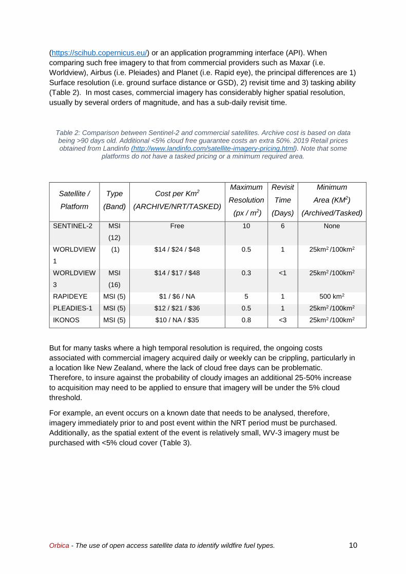
(Table 2). In most cases, commercial imagery has considerably higher spatial resolution,
usually by several orders of magnitude, and has a sub-daily revisit time.
Table 2: Comparison between Sentinel-2 and commercial satellites. Archive cost is based on data being >90 days old. Additional <5% cloud free guarantee costs an extra 50%. 2019 Retail prices obtained from Landinfo (http://www.landinfo.com/satellite-imagery-pricing.html). Note that some
platforms do not have a tasked pricing or a minimum required area.
Satellite /
Platform
Type
(Band)
Cost per Km2
(ARCHIVE/NRT/TASKED)
Maximum
Resolution
(px / m2)
Revisit
Time
(Days)
Minimum
Area (KM2)
(Archived/Tasked)
SENTINEL-2 MSI
(12)
Free 10 6 None
WORLDVIEW
1
(1) $14 / $24 / $48 0.5 1 25km2 /100km2
WORLDVIEW
3
MSI
(16)
$14 / $17 / $48 0.3 <1 25km2 /100km2
RAPIDEYE MSI (5) $1 / $6 / NA 5 1 500 km2
PLEADIES-1 MSI (5) $12 / $21 / $36 0.5 1 25km2 /100km2
IKONOS MSI (5) $10 / NA / $35 0.8 <3 25km2 /100km2
But for many tasks where a high temporal resolution is required, the ongoing costs
associated with commercial imagery acquired daily or weekly can be crippling, particularly in
a location like New Zealand, where the lack of cloud free days can be problematic.
Therefore, to insure against the probability of cloudy images an additional 25-50% increase
to acquisition may need to be applied to ensure that imagery will be under the 5% cloud
threshold.
For example, an event occurs on a known date that needs to be analysed, therefore,
imagery immediately prior to and post event within the NRT period must be purchased.
Additionally, as the spatial extent of the event is relatively small, WV-3 imagery must be
purchased with <5% cloud cover (Table 3).
Orbica - The use of open access satellite data to identify wildfire fuel types. 11
Table 3: Example costing for a simple, prior/post RS task. Prices based on Landpro.com (4/13/2018)
Imagery prior to event: $29 usd per km2 (minimum 100km2) = $2900 usd
<5% cloud cover guarantee = $1450 usd
Imagery post event: $29 usd per km2 (minimum 100km2) = $2900 usd
<5% cloud cover guarantee = $1450 usd
Converting it from USD to NZD we get a cost of ~$13,000. An expensive exercise, even if
treated as a worst-case scenario. Given this cost, it is easy to imagine organisations being
extremely cautious in such an approach, thus the use of lower resolution imagery, even with
their caveats, can be a powerful alternative.
Even with lower spatial and temporal resolution, the open access imagery of platforms such
as Sentinel can provide a sandbox for testing and building RS solutions for land change
monitoring that is de-risked compared to that of commercial imagery (Figure 1).
Figure 1: Example of commercial 0.6m Quickbird-2 (left) vs open access 10m Sentinel-2 (right) imagery for an area south of Whangamata in the Bay of Plenty. Approximately ten years separate the
two images (QB-2 2009, S-2 2019).
If the target of interest is large enough and the period of identification (i.e. dates pre- and
post-event) is coarse enough, such data is a viable solution even within a production
environment. Therefore, for the purposes of this report, the use of Sentinel-2 imagery
provides a perfect source of data to test: whether open access imagery can be used for
vegetation classification? and is it a viable alternative to commercial imagery?
Orbica - The use of open access satellite data to identify wildfire fuel types. 12
2.1. SENTINEL-2 MULTISPECTRAL IMAGERY (MSI)
Optical multispectral imagery (MSI) is a passive remote sensing technique and requires
some form of illumination (i.e. the sun) to achieve results. Therefore, this data is not only
constrained to daytime use but is also heavily affected by cloud cover. This is in stark
contrast to the radar data acquired by the Sentinel-1 platform, in which actively emitted C-
band microwaves self-illuminate a scene and clouds do not affect the data.
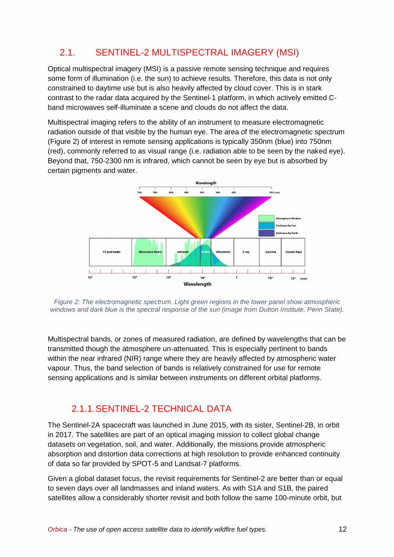
Multispectral imaging refers to the ability of an instrument to measure electromagnetic
radiation outside of that visible by the human eye. The area of the electromagnetic spectrum
(Figure 2) of interest in remote sensing applications is typically 350nm (blue) into 750nm
(red), commonly referred to as visual range (i.e. radiation able to be seen by the naked eye).
Beyond that, 750-2300 nm is infrared, which cannot be seen by eye but is absorbed by
certain pigments and water.
Figure 2: The electromagnetic spectrum. Light green regions in the lower panel show atmospheric windows and dark blue is the spectral response of the sun (image from Dutton Institute, Penn State).
Multispectral bands, or zones of measured radiation, are defined by wavelengths that can be
transmitted though the atmosphere un-attenuated. This is especially pertinent to bands
within the near infrared (NIR) range where they are heavily affected by atmospheric water
vapour. Thus, the band selection of bands is relatively constrained for use for remote
sensing applications and is similar between instruments on different orbital platforms.
2.1.1. SENTINEL-2 TECHNICAL DATA
The Sentinel-2A spacecraft was launched in June 2015, with its sister, Sentinel-2B, in orbit
in 2017. The satellites are part of an optical imaging mission to collect global change
datasets on vegetation, soil, and water. Additionally, the missions provide atmospheric
absorption and distortion data corrections at high resolution to provide enhanced continuity
of data so far provided by SPOT-5 and Landsat-7 platforms.
Given a global dataset focus, the revisit requirements for Sentinel-2 are better than or equal
to seven days over all landmasses and inland waters. As with S1A and S1B, the paired
satellites allow a considerably shorter revisit and both follow the same 100-minute orbit, but
Orbica - The use of open access satellite data to identify wildfire fuel types. 13
180° apart. This allows maximum coverage, and each satellite collects ~149 million km2 of
imagery per orbit (approximately 1.6 Tb). Therefore, in a single day (~15 orbits), the
Sentinel-2 spacecraft transmit ~50 Tb of raw data back to earth via a combination of
dedicated ground stations and orbital relay satellites.
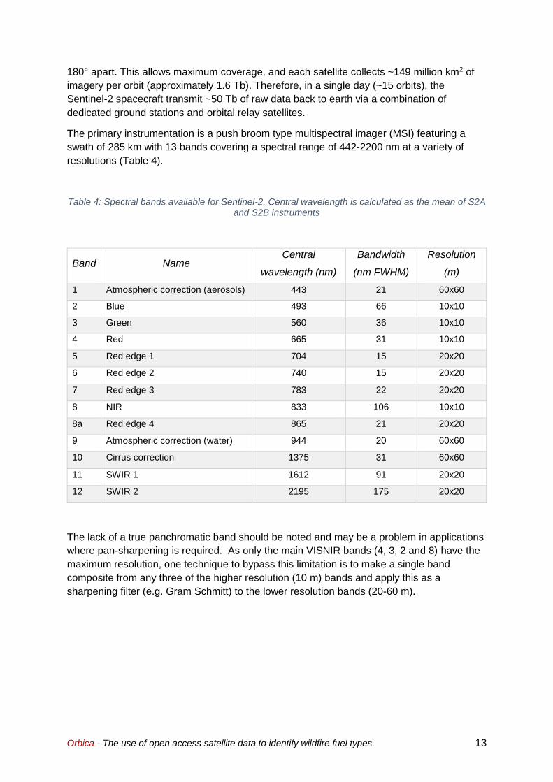
The primary instrumentation is a push broom type multispectral imager (MSI) featuring a
swath of 285 km with 13 bands covering a spectral range of 442-2200 nm at a variety of
resolutions (Table 4).
Table 4: Spectral bands available for Sentinel-2. Central wavelength is calculated as the mean of S2A and S2B instruments
Band Name Central
wavelength (nm)
Bandwidth
(nm FWHM)
Resolution
(m)
1 Atmospheric correction (aerosols) 443 21 60x60
2 Blue 493 66 10x10
3 Green 560 36 10x10
4 Red 665 31 10x10
5 Red edge 1 704 15 20x20
6 Red edge 2 740 15 20x20
7 Red edge 3 783 22 20x20
8 NIR 833 106 10x10
8a Red edge 4 865 21 20x20
9 Atmospheric correction (water) 944 20 60x60
10 Cirrus correction 1375 31 60x60
11 SWIR 1 1612 91 20x20
12 SWIR 2 2195 175 20x20
The lack of a true panchromatic band should be noted and may be a problem in applications
where pan-sharpening is required. As only the main VISNIR bands (4, 3, 2 and 8) have the
maximum resolution, one technique to bypass this limitation is to make a single band
composite from any three of the higher resolution (10 m) bands and apply this as a
sharpening filter (e.g. Gram Schmitt) to the lower resolution bands (20-60 m).

Orbica - The use of open access satellite data to identify wildfire fuel types. 14
2.2. DATA DISSEMINATION AND ACCESS
2.2.1. COPERNICUS OPEN ACCESS HUB (COH)
Given the purpose of the Copernicus programme is to provide open data for Earth
observation, the dissemination and analysis tools are a key component. As the data itself is
open source, several third-party companies have emerged as data distributors, with their
selling point being easier data access, via web services, or easier analytics, via APIs. The
following discussion looks at the advantages and disadvantages of one such system,
Synergises’ Sentinel-hub (https://sentinel-hub.com/) versus the Copernicus open access
hub.
2.2.2. SENTINEL HUB
A different approach to data access is provided by third party companies such as Sinergise.
The Sinergise paradigm is that instead of end-users interacting with, and processing, raw
data from ESA, users have access to curated global datasets. Sentinel-Hub (www.sentinel-
hub.com) provides users a more simplistic way to view data, but also a fully featured python
API with machine learning, data cube storage and analytic tools. Sentinel Hub is a paid
service that has several tiers, that provide a range of processing units and access based on
research / commercial use (Table 5).
Table 5: Pricing breakdown for Sentinel Hub as of February 2020 (https://sentinel-hub.com/pricing-plans)
Get
Started
Individual
(non-
commercial)
Individual
(commercial)
Enterprise
(Basic)
Enterprise
(Enlarged)
Price Free ~$277 nzd/yr ~$1700
nzd/yr
~$10000
nzd/yr
~$20000 nzd/yr
Raw data
download N Y Y Y Y
Web services N Y Y Y Y
API N Y Y Y Y
Rate limits
(Requests per
minute/ processing
units per month)
NA 300/30k 500/50k 600/200k 600/500k
Non-Commercial
use Y Y Y Y Y
Number of users 1 1 1 ∞ ∞
Mobile apps N N N Y Y

Orbica - The use of open access satellite data to identify wildfire fuel types. 15
2.2.3. SERVICES
A key strength of the Sentinel Hub suite of tools is the ability to use rendered on the fly
imagery. While the initial selection is limited, a user can import a range of pre-existing or
their own custom spectral indices. Within Sentinel Hub, a configuration tool allows the
creation of multiple instances, each with their own API key, that can include any number of
Web mapping service (WMS) endpoints. Each of which contains a JavaScript configuration
script that can be filtered by date and tile-level cloud cover. The custom configuration script
also allows a user to define:
• Histogram stretching
• Visualisation type
• Symbology
• Band combination.
Sentinel Hub also provides several easy to access web-based tools. Sentinel playground
and EO browser are the “Google Maps” of satellite data in the Sentinel-Hub world. Sentinel
playground (https://sentinel-hub.com/explore/sentinel-playground) is the most simplistic and
provides the user with a series of pre-processed data that can be explored. Filtering is basic,
by date, location, and cloud cover, but playground gives instant access to a variety of global
Sentinel-2 visualised data products (Figure 3).
Figure 3: Sentinel Playground screen capture of Tripoli, Libya on the 12/6/2016. Data is a false colour (12, 4, 2) SWIR composite that highlights the regional geology.
EO-Brower is a more analytically focused product and requires a Sinergise account to
access (Figure 4). As well as Sentinel platforms (S1, S2, S3 and S5P), several other freely
accessible satellite datasets can be browsed and analysed (Table 6). Additionally, several
other products, including the ASTER global elevation model, are available via the NASA
Global Imagery Browser Service (GIBS,
https://wiki.earthdata.nasa.gov/pages/viewpage.action?pageId=2228230).
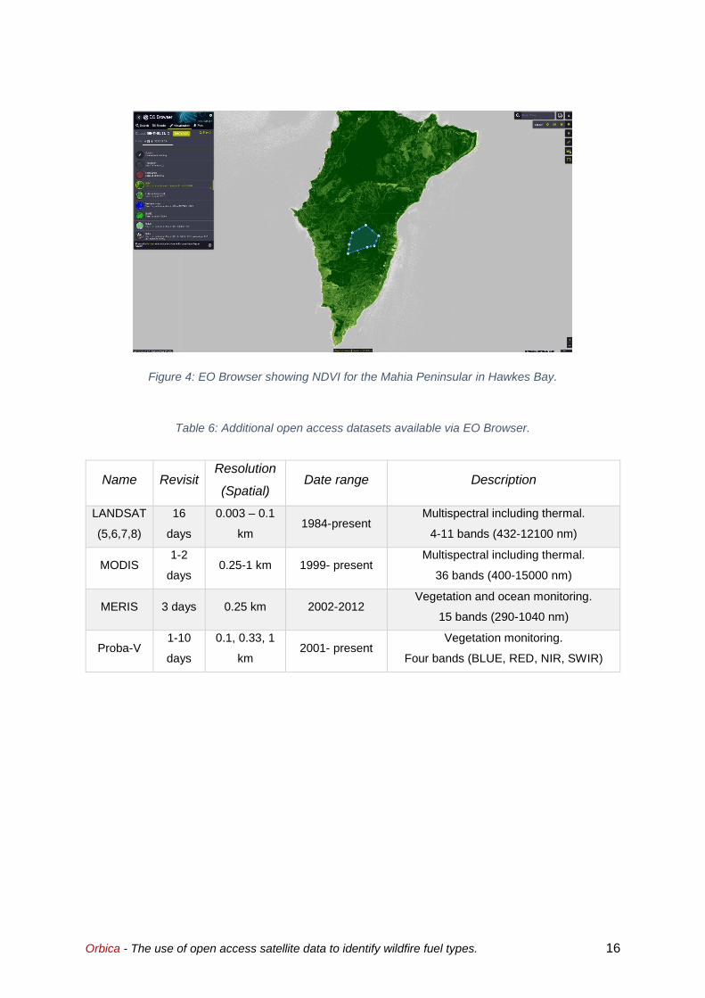
Orbica - The use of open access satellite data to identify wildfire fuel types. 16
Figure 4: EO Browser showing NDVI for the Mahia Peninsular in Hawkes Bay.
Table 6: Additional open access datasets available via EO Browser.
Name Revisit Resolution
(Spatial) Date range Description
LANDSAT
(5,6,7,8)
16
days
0.003 – 0.1
km 1984-present
Multispectral including thermal.
4-11 bands (432-12100 nm)
MODIS 1-2
days 0.25-1 km 1999- present
Multispectral including thermal.
36 bands (400-15000 nm)
MERIS 3 days 0.25 km 2002-2012 Vegetation and ocean monitoring.
15 bands (290-1040 nm)
Proba-V 1-10
days
0.1, 0.33, 1
km 2001- present
Vegetation monitoring.
Four bands (BLUE, RED, NIR, SWIR)
Orbica - The use of open access satellite data to identify wildfire fuel types. 17
3. LANDCOVER DATABASE COMPARISON
A key dataset used in Prometheus and FENZs wildfire threat modelling is the NZ Land
Cover Database (LCDB) produced by Landcare Research-Manaaki Whenua. It is a
comprehensive land cover classification, grouping together similar land cover types based
on satellite imagery into a shared taxonomy.
Several important updates have been made since the release of the dataset, particularly
versions 2 (2002) and 5 (2020). Although version 5 is the most up to date and provides the
most accurate picture of a real vegetation cover, the decision was made to integrate and
merge several subclasses in later releases (Table 7).
This has led to a situation where the most up to date dataset in a spatial context (v5 in 2020)
does not contain the required resolution in discrete land classes. The trade-off for having
more detailed land cover classes is that data is out of data by ~18 years, increasing the
ambiguity of the fuel types which therefore reduces the ability to accurately model fire
damage potential.
FENZ have been primarily using LCDB2 as inputs into their threat assessment model, due to
the higher resolution of land classes, and thus possible wildfire fuel types. But the
acknowledged “elephant” in the room is the age and thus validity of the data’s spatial extent.
Although version 5 is recognised as being more up to date, the merging of subclasses,
particularly in the “Exotic forestry” class is a stumbling block to the adoption of LCDB5.

Orbica - The use of open access satellite data to identify wildfire fuel types. 18
Table 7: A comparison of LCDB class codes between versions 2 and 4
LCDB V2 LCDB V4 AND ONWARD Class Code Class Name Class Code Class Name
OTHER 0 Not land (used in V5 onwards)
ARTIFICIAL
SURFACES
1 Built up area (Settlement) 1 Built up area (Settlement)
2 Urban parkland / Open space 2 Urban parkland / Open space
3 Surface mine 6 Surface mines and dumps
4 Dump
5 Transportation infrastructure 5 Transportation infrastructure
BARE OR
LIGHTLY
VEGETATED
SURFACES
10 Coastal sand and gravel 10 Sand and gravel
11 River and lakeshore gravel and
rock
16 Gravel and rock
13 Alpine gravel and rock
12 Landslide 12 Landslide
14 Permanent snow and ice 14 Permanent snow and ice
15 Alpine grass/herb field 15 Alpine grass/herb field
WATER
BODIES
20 Lake and pond 20 Lake and pond
21 River 21 River
22 Estuarine open water 22 Estuarine open water
CROPLAND
30 Short-rotation cropland 30 Short-rotation cropland
31 Vineyard 33 Orchard, vineyard, and other perennial
crops
32 Orchard and other perennial crops
GRASSLAND
,
SEDGELAND,
AND
MARSHLAND
40 High producing exotic grassland 40 High producing exotic grassland
41 Low producing grassland 41 Low producing grassland
42 Tall tussock grassland 42 Tall tussock grassland
44 Depleted grassland 44 Depleted grassland
45 Herbaceous freshwater vegetation 45 Herbaceous freshwater vegetation
46 Herbaceous saline vegetation 46 Herbaceous saline vegetation
47 Flaxland 47 Flaxland
SCRUB AND
SHRUBLAND
S
50 Fern land 50 fenland
51 Gorse and/or Broom 51 Gorse and/or Broom
52 Manuka and/or Kanuka 52 Manuka and/or Kanuka
53 Matagouri 58 Matagouri and/or grey scrub
57 Grey scrub
54 Broadleaf indigenous hardwoods 54 Broadleaf indigenous hardwoods
55 Sub-alpine shrubland 55 Sub-alpine shrubland
56 Mixed-exotic shrubland 56 Mixed-exotic shrubland
55 Peat shrubland (Chatham Island
only)
80 Peat shrubland (Chatham Island only)
56 Dune shrubland (Chatham Island
only)
81 Dune shrubland (Chatham Island only)
FOREST
60 Minor shelterbelts 71 Exotic forests
61 Major shelterbelts
62 Afforestation (not imaged)
63 Afforestation (imaged post-lcdb1)
65 Pine forest – open canopy
66 Pine forest – closed canopy
67 Other exotic forest
64 Forest – harvested 64 Forest – harvested
68 Deciduous hardwoods 68 Deciduous hardwoods
69 Indigenous forest 69 Indigenous forest
70 Mangrove 70 Mangrove
Orbica - The use of open access satellite data to identify wildfire fuel types. 19
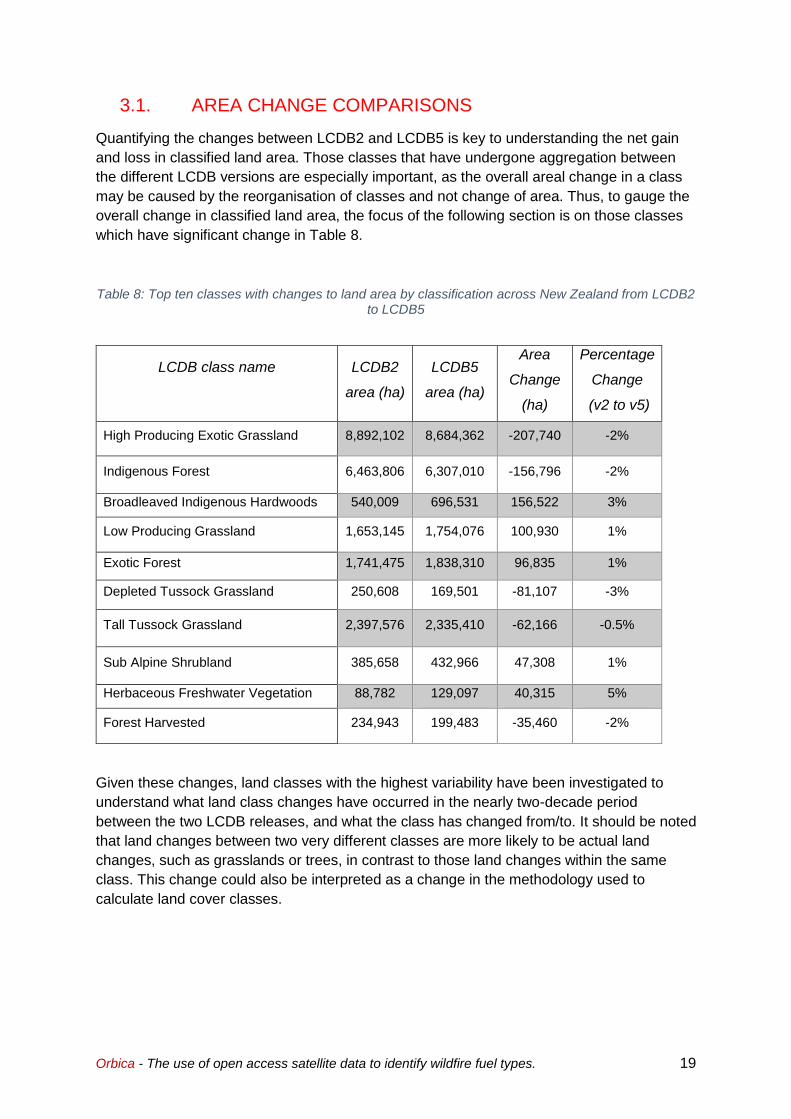
3.1. AREA CHANGE COMPARISONS
Quantifying the changes between LCDB2 and LCDB5 is key to understanding the net gain
and loss in classified land area. Those classes that have undergone aggregation between
the different LCDB versions are especially important, as the overall areal change in a class
may be caused by the reorganisation of classes and not change of area. Thus, to gauge the
overall change in classified land area, the focus of the following section is on those classes
which have significant change in Table 8.
Table 8: Top ten classes with changes to land area by classification across New Zealand from LCDB2 to LCDB5
Given these changes, land classes with the highest variability have been investigated to
understand what land class changes have occurred in the nearly two-decade period
between the two LCDB releases, and what the class has changed from/to. It should be noted
that land changes between two very different classes are more likely to be actual land
changes, such as grasslands or trees, in contrast to those land changes within the same
class. This change could also be interpreted as a change in the methodology used to
calculate land cover classes.
LCDB class name
LCDB2
area (ha)
LCDB5
area (ha)
Area
Change
(ha)
Percentage
Change
(v2 to v5)
High Producing Exotic Grassland 8,892,102 8,684,362 -207,740 -2%
Indigenous Forest 6,463,806 6,307,010 -156,796 -2%
Broadleaved Indigenous Hardwoods 540,009 696,531 156,522 3%
Low Producing Grassland 1,653,145 1,754,076 100,930 1%
Exotic Forest 1,741,475 1,838,310 96,835 1%
Depleted Tussock Grassland 250,608 169,501 -81,107 -3%
Tall Tussock Grassland 2,397,576 2,335,410 -62,166 -0.5%
Sub Alpine Shrubland 385,658 432,966 47,308 1%
Herbaceous Freshwater Vegetation 88,782 129,097 40,315 5%
Forest Harvested 234,943 199,483 -35,460 -2%
Orbica - The use of open access satellite data to identify wildfire fuel types. 20
3.1.1. GREATEST ABSOLUTE CHANGE IN AREA
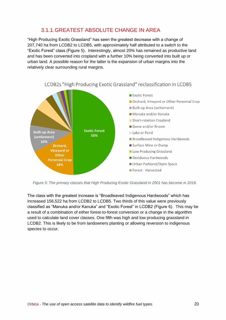
“High Producing Exotic Grassland” has seen the greatest decrease with a change of
207,740 ha from LCDB2 to LCDB5, with approximately half attributed to a switch to the
“Exotic Forest” class (Figure 5). Interestingly, almost 20% has remained as productive land
and has been converted into cropland with a further 10% being converted into built up or
urban land. A possible reason for the latter is the expansion of urban margins into the
relatively clear surrounding rural margins.
The class with the greatest increase is “Broadleaved Indigenous Hardwoods” which has
increased 156,522 ha from LCDB2 to LCDB5. Two thirds of this value were previously
classified as “Manuka and/or Kanuka” and “Exotic Forest” in LCDB2 (Figure 6). This may be
a result of a combination of either forest-to-forest conversion or a change in the algorithm
used to calculate land cover classes. One fifth was high and low producing grassland in
LCDB2. This is likely to be from landowners planting or allowing reversion to indigenous
species to occur.
Figure 5: The primary classes that High Producing Exotic Grassland in 2001 has become in 2018.

Orbica - The use of open access satellite data to identify wildfire fuel types. 21
3.1.2. GREATEST RELATIVE CHANGE IN AREA
The greatest relative decrease in area has occurred within the “Depleted Grassland” class
which has decreased 3% or 81,107 ha from LCDB2 to LCDB5. Almost 90% remains as
grassland although has been reclassified as either low or high producing (Figure 7). A likely
explanation for this change may be due to landowners improving grass quality or a change
in the algorithm used to calculate land cover classes.
“Herbaceous Freshwater Vegetation” is the class with greatest relative increase in area, with
an increase of 5%, or 40,315 ha) from LCDB2 to LCDB5 (Figure 8). Half of this increase
came from land previously classified as Deciduous Hardwoods, with much of the remaining
area previously classed as grassland or lake/pond. The change in area is likely the result of
land being reverted or converted to wetlands and water drainage areas.
Figure 6: Chart shows what Broadleaved Indigenous Hardwoods in 2018 were in 2001, excluding Broadleaved Indigenous Hardwoods

Orbica - The use of open access satellite data to identify wildfire fuel types. 22
Figure 7: Depleted Grasslands conversion from 2001 to 2018.
Figure 8: Herbaceous Freshwater Vegetation conversion from 2001 to 2018, excluding Herbaceous Freshwater Vegetation
Orbica - The use of open access satellite data to identify wildfire fuel types. 23
4. CASE STUDY 1: EXOTIC FORESTRY
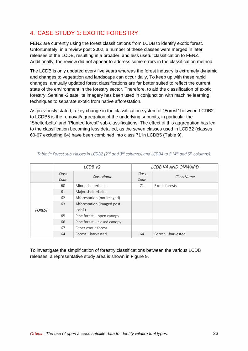
FENZ are currently using the forest classifications from LCDB to identify exotic forest.
Unfortunately, in a review post 2002, a number of these classes were merged in later
releases of the LCDB, resulting in a broader, and less useful classification to FENZ.
Additionally, the review did not appear to address some errors in the classification method.
The LCDB is only updated every five years whereas the forest industry is extremely dynamic
and changes to vegetation and landscape can occur daily. To keep up with these rapid
changes, annually updated forest classifications are far better suited to reflect the current
state of the environment in the forestry sector. Therefore, to aid the classification of exotic
forestry, Sentinel-2 satellite imagery has been used in conjunction with machine learning
techniques to separate exotic from native afforestation.
As previously stated, a key change in the classification system of “Forest” between LCDB2
to LCDB5 is the removal/aggregation of the underlying subunits, in particular the
“Shelterbelts” and “Planted forest” sub-classifications. The effect of this aggregation has led
to the classification becoming less detailed, as the seven classes used in LCDB2 (classes
60-67 excluding 64) have been combined into class 71 in LCDB5 (Table 9).
Table 9: Forest sub-classes in LCDB2 (2nd and 3rd columns) and LCDB4 to 5 (4th and 5th columns).
LCDB V2 LCDB V4 AND ONWARD
Class
Code Class Name
Class
Code Class Name
FOREST
60 Minor shelterbelts 71 Exotic forests
61 Major shelterbelts
62 Afforestation (not imaged)
63 Afforestation (imaged post-
lcdb1)
65 Pine forest – open canopy
66 Pine forest – closed canopy
67 Other exotic forest
64 Forest – harvested 64 Forest – harvested
To investigate the simplification of forestry classifications between the various LCDB
releases, a representative study area is shown in Figure 9.

Orbica - The use of open access satellite data to identify wildfire fuel types. 24
Figure 9: LCDB2 (left) showing forestry sub-classes – light green: open canopy pine, dark green: closed canopy pine, yellow: other exotic forest, pink: afforested varieties. LCDB5 (right) showing the
exotic forestry class. Blue represents harvested areas in both.
On first comparison, it is clear the delineation of different forestry fuel classes has been lost,
but the overall extent of forestry has undergone little change. As a result, there will be a
negative impact on the ability to determine fire behaviour in the different forestry fuel
classes. The blue areas identified as harvested are accurately represented when compared
with aerial imagery.
The Ministry for the Environment’s Land-use and Carbon Analysis System (LUCAS) 2016
Forest classification also shows similar forest extents. Unfortunately, LUCAS only identifies
forestry as pre-1990 or post-1989 and does not identify harvested areas.
As well as issues surrounding the aggregation of classes, there are also occurrences of
legacy errors in classification methodology that persist through multiple revisions of the
LCDB.
Observed throughout the datasets, there are cases where algorithms used to calculate
classes are not correctly identifying forestry. For example, there are parcels that were
identified as “Exotic Forest” in LCDB2 and remain as such in LCDB5, yet they were not
visible as exotic forest in 2018. This appears to be a legacy issue where at one point in time,
the land may have been correctly, or incorrectly, classified as exotic forest and in later
iterations the algorithm has not picked up on land use change, yet the classification remains.
An example of this is shown below in Figure 10, where the two pink highlighted parcels are
defined as Exotic Forest in LCDB5, but the underlying imagery from 2018 shows no forestry.
Orbica - The use of open access satellite data to identify wildfire fuel types. 25
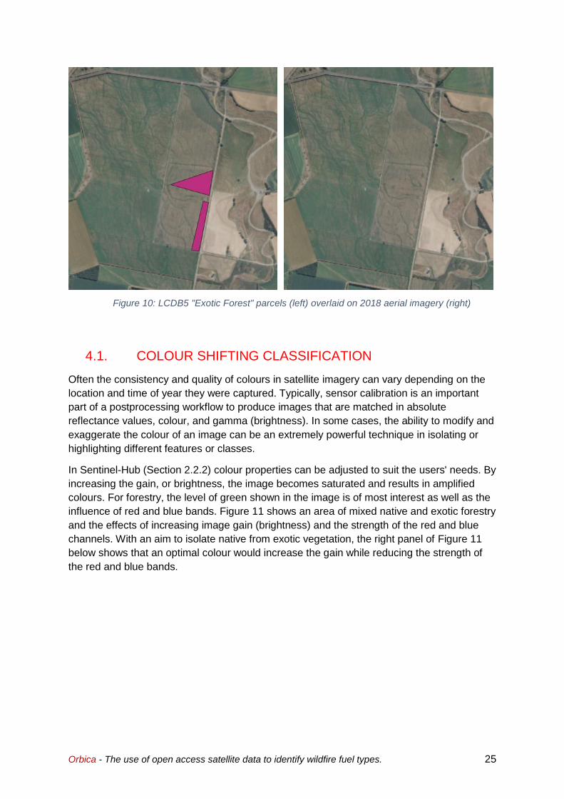
4.1. COLOUR SHIFTING CLASSIFICATION
Often the consistency and quality of colours in satellite imagery can vary depending on the
location and time of year they were captured. Typically, sensor calibration is an important
part of a postprocessing workflow to produce images that are matched in absolute
reflectance values, colour, and gamma (brightness). In some cases, the ability to modify and
exaggerate the colour of an image can be an extremely powerful technique in isolating or
highlighting different features or classes.
In Sentinel-Hub (Section 2.2.2) colour properties can be adjusted to suit the users' needs. By
increasing the gain, or brightness, the image becomes saturated and results in amplified
colours. For forestry, the level of green shown in the image is of most interest as well as the
influence of red and blue bands. Figure 11 shows an area of mixed native and exotic forestry
and the effects of increasing image gain (brightness) and the strength of the red and blue
channels. With an aim to isolate native from exotic vegetation, the right panel of Figure 11
below shows that an optimal colour would increase the gain while reducing the strength of
the red and blue bands.
Figure 10: LCDB5 "Exotic Forest" parcels (left) overlaid on 2018 aerial imagery (right)

Orbica - The use of open access satellite data to identify wildfire fuel types. 26
Figure 11: The effects of altering image gain on forested areas. High gain (left), medium to high gain (middle), and high gain with low red and blue values (right).
4.2. DEEP LEARNING CLASSIFICATION
To trial an artificial intelligence approach to image classification and segmentation, a
commercially planted exotic forest area in Tasman has been selected. Spatial data of
forestry stands provided by Onefortyone (https://onefortyone.com/) is for an AOI that
contains a mix of ages within an active plantation initially established in 1936. The current
crop is second or third rotation (Figure 12).
.
Figure 12: The Golden Downs study area identified by Onefortyone that contains a mix of species and
rotations.
Orbica - The use of open access satellite data to identify wildfire fuel types. 27
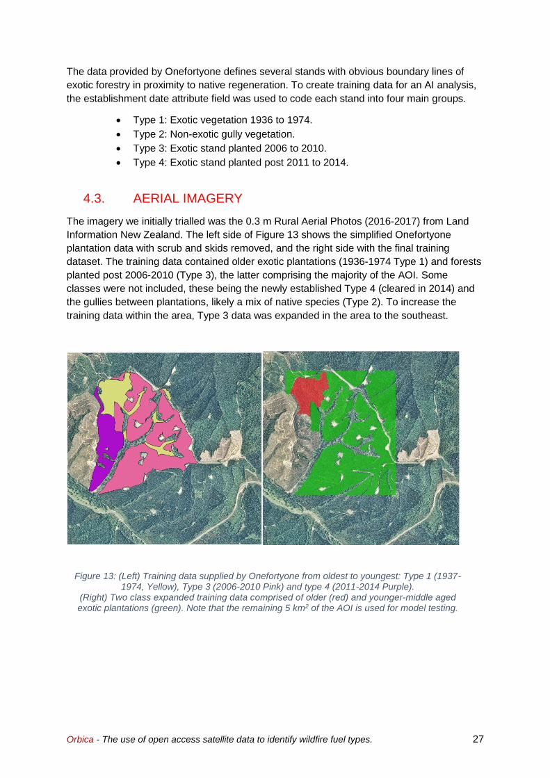
The data provided by Onefortyone defines several stands with obvious boundary lines of
exotic forestry in proximity to native regeneration. To create training data for an AI analysis,
the establishment date attribute field was used to code each stand into four main groups.
• Type 1: Exotic vegetation 1936 to 1974.
• Type 2: Non-exotic gully vegetation.
• Type 3: Exotic stand planted 2006 to 2010.
• Type 4: Exotic stand planted post 2011 to 2014.
4.3. AERIAL IMAGERY
The imagery we initially trialled was the 0.3 m Rural Aerial Photos (2016-2017) from Land
Information New Zealand. The left side of Figure 13 shows the simplified Onefortyone
plantation data with scrub and skids removed, and the right side with the final training
dataset. The training data contained older exotic plantations (1936-1974 Type 1) and forests
planted post 2006-2010 (Type 3), the latter comprising the majority of the AOI. Some
classes were not included, these being the newly established Type 4 (cleared in 2014) and
the gullies between plantations, likely a mix of native species (Type 2). To increase the
training data within the area, Type 3 data was expanded in the area to the southeast.
Figure 13: (Left) Training data supplied by Onefortyone from oldest to youngest: Type 1 (1937-1974, Yellow), Type 3 (2006-2010 Pink) and type 4 (2011-2014 Purple).
(Right) Two class expanded training data comprised of older (red) and younger-middle aged exotic plantations (green). Note that the remaining 5 km2 of the AOI is used for model testing.
Orbica - The use of open access satellite data to identify wildfire fuel types. 28
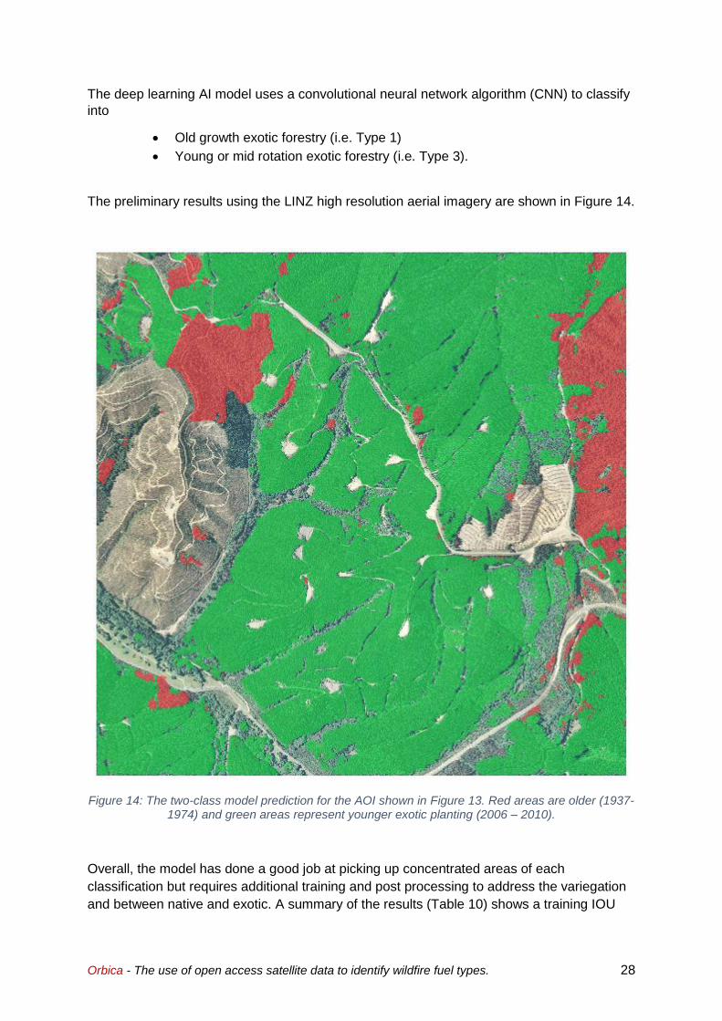
The deep learning AI model uses a convolutional neural network algorithm (CNN) to classify
into
• Old growth exotic forestry (i.e. Type 1)
• Young or mid rotation exotic forestry (i.e. Type 3).
The preliminary results using the LINZ high resolution aerial imagery are shown in Figure 14.
Figure 14: The two-class model prediction for the AOI shown in Figure 13. Red areas are older (1937-1974) and green areas represent younger exotic planting (2006 – 2010).
Overall, the model has done a good job at picking up concentrated areas of each
classification but requires additional training and post processing to address the variegation
and between native and exotic. A summary of the results (Table 10) shows a training IOU
Orbica - The use of open access satellite data to identify wildfire fuel types. 29
(intersection over union) accuracy of ~93%, and a final visual QA of the results by a human
analyst suggest a final testing accuracy of 85%.
Table 10: Model run times and IOU accuracy scores.
Training Validation Testing
Number of images
used 1
(1500 smaller patches)
1
(340 smaller patches)
1
(5000 smaller patches)
Time in minutes 120 min 1 min 2 min
Model loss
(Error Rate %) 0.0128 0.0138
Accuracy (IOU) 0.9345 0.9073 0.85 (QA/QC)
Given the limited amount of training data (one tile), the CNN model did extremely well in
identifying native vs exotic forests within the AOI. The ability of CNN to incorporate the
context of the training pixels (i.e. shape, texture, colour variation) to learn from shows the
strength of the technique in this application.
4.4. SENTINEL IMAGERY
The use of the LINZ imagery combined with CNN algorithms proved that identifying forestry
classes, and possibly age, can be achieved using high resolution imagery. Unfortunately,
this may not be realistically achievable using Sentinel satellite data, due to its significantly
lower resolution. To additionally test this hypothesis, several Sentinel-2 raw and derived data
products acquired on 17/08/2019 were also tested using the same training AOI.
The Normalised Difference Vegetation Index (NDVI) is a spectral index that employs
Sentinel-2 very near infrared (B8) and red (B4) bands.
𝑁𝐷𝑉𝐼 =(𝑁𝐼𝑅(𝐵8) − 𝑅𝐸𝐷(𝐵4))
(𝑁𝐼𝑅(𝐵8) + 𝑅𝐸𝐷(𝐵4))
The NDVI shows the relative reflectance of chlorophyll absorption and is sensitive to
variations in both chlorophyll concentrations and leaf area. Therefore, it provides a plant
health metric that is generally unaffected by illumination variations and soil effects.
As shown in Figure 15, the AOI of forestry, supplied by Onefortyone and used in the
previous examples, shows brighter values (heathier vegetation) in the younger exotic
plantings (Figure 15, right bottom) and darker values in the older exotic vegetation (Figure
15, right top).

Orbica - The use of open access satellite data to identify wildfire fuel types. 30
Another method to highlight changes in vegetation is the use of False Colour Infrared
In this technique, instead of calculating an index using a combination of bands, the
visualised bands are swapped around. So instead of a true colour representation of the data
where:
𝑅𝐺𝐵 = 𝑅(𝐵4) 𝐺(𝐵3) 𝐵(𝐵2)
Bands are swapped around, and an infrared band is included. So that the red band colour is
replaced with NIR, green with red, and blue with green.
𝐹𝐶𝐼𝑅 = 𝑅(𝐵8) 𝐺(𝐵4) 𝐵(𝐵3)
The advantage of this technique is that it can highlight the spectral difference within an AOI
and thus aid in the interpretation of complex imagery. As with the NDVI technique, False-
colour infrared (FCIR) for the area (Figure 16) shows only minor visual changes between
type 1 and type 2 forestry. This lack of differentiation between bands is also observed in the
true colour imagery (Figure 17), where shadowing may play a role.
Figure 15: (Left) Normalised Difference Vegetation Index (NDVI) of the AOI (white box) overlain with the Onefortyone training data (Black). Side panels show areas of old-growth (Right top) and younger (right bottom) exotic forestry. Darker colours show less healthy
vegetation and bare ground, and the lighter the reverse.

Orbica - The use of open access satellite data to identify wildfire fuel types. 31
Given the lack of pixel resolution in the Sentinel-2 imagery (10-60 m) compared to that of the
LINZ 0.03 m imagery and the lack of differentiation between the various band combinations
presented above, can machine learning techniques be employed?
Unsupervised K-means clustering was assessed as a method to group the pixel values into
discrete units. Unfortunately, the use of CNN requires far more training data for use with the
Sentinel imagery. The provided AOI is approximately 15000 Sentinel-2 pixels compared to
the 17 million LINZ aerial pixels found in the same extent. These values mean that the same
Figure 16: (Left) False-colour infrared (FCIR) of the AOI (white box) overlain with the Onefortyone training data (Black). Side panels show areas of old-growth (right top) and
younger (right bottom) exotic forestry.
Figure 17: (Left) True colour (RGB) of the AOI (white box) overlain with the Onefortyone training data (Black). Side panels show areas of old-growth (right top) and younger (right bottom) exotic
forestry.
Orbica - The use of open access satellite data to identify wildfire fuel types. 32
CNN algorithm has orders of magnitude less pixels to learn off, which in the context of shape
and texture can radically reduce the efficiency of the model.
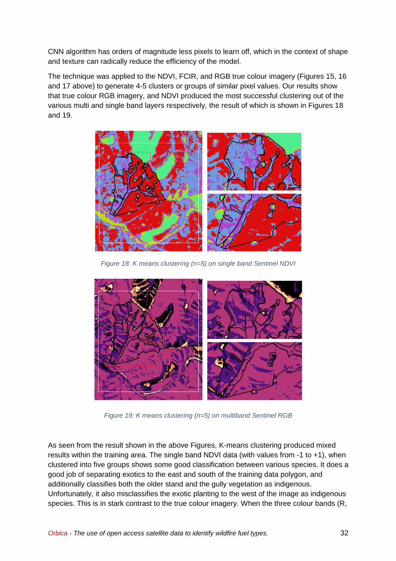
The technique was applied to the NDVI, FCIR, and RGB true colour imagery (Figures 15, 16
and 17 above) to generate 4-5 clusters or groups of similar pixel values. Our results show
that true colour RGB imagery, and NDVI produced the most successful clustering out of the
various multi and single band layers respectively, the result of which is shown in Figures 18
and 19.
Figure 18: K means clustering (n=5) on single band Sentinel NDVI
Figure 19: K means clustering (n=5) on multiband Sentinel RGB
As seen from the result shown in the above Figures, K-means clustering produced mixed
results within the training area. The single band NDVI data (with values from -1 to +1), when
clustered into five groups shows some good classification between various species. It does a
good job of separating exotics to the east and south of the training data polygon, and
additionally classifies both the older stand and the gully vegetation as indigenous.
Unfortunately, it also misclassifies the exotic planting to the west of the image as indigenous
species. This is in stark contrast to the true colour imagery. When the three colour bands (R,

Orbica - The use of open access satellite data to identify wildfire fuel types. 33
G and B, all with 8-bit values from 0-255) are clustered into four groups, the K means
method performs badly within the training area. Basically, classifying into slope aspect and
shadowing (Figure 19 above).
Overall, the use of machine learning, and geostatistical techniques do show promise in the
detection of indigenous vs native forestry, and possibly the age of exotic forestry. Although
the above is a simple example of machine learning, and supplied only with a limited training
dataset, it demonstrates the power of such algorithms applied to satellite imagery.
Colour shifting to enhance specific regions of greenness, appears to be a useful tool in
separating, albeit qualitatively, tree species in homogenous plantations or stands. In contrast
the use of CNN deep learning techniques, is particularly powerful and even a relatively small
training dataset can be used on high resolution imagery to produce mapping of stands at the
>80% level.
Unfortunately, training data with far larger extents are required to apply deep learning
techniques to sentinel imagery, and the alternative, K-means clustering, modelled clusters
relatively poorly compared to the CNN results.
To increase the accuracy and to assist with model training for afforested exotic forest and
exotic forest blocks of different ages several additional points can be considered.
• The data supplied by Onefortyone was extremely valuable, and therefore it would be
extremely beneficial to have more of these areas identified by forestry companies.
These data, when used as model inputs, are precise and validated, eliminating
assumptions made when selecting forest for different classifications. As expected, to
leverage the maximum amount of value from such data, it would need to overlap with
the acquisition of the imagery to effectively train the model. It is likely forestry data
would only be required for the initial training of the model and not required on an
ongoing basis, except when the model requires tuning.
• The inclusion of additional bands of satellite imagery. While the use of Sentinel-2
imagery in this report has typically been limited to true colour (3 band) imagery, 14
bands of various wavelength are available to be used.
Orbica - The use of open access satellite data to identify wildfire fuel types. 34
5. CASE STUDY 2: SHELTERBELT DETECTION
Shelterbelts (e.g. windbreaks or hedgerows) are important infrastructure on farms across
New Zealand as they provide protection from the elements to livestock and agricultural
crops. Typically comprised of exotic species such as radiata pine or macrocarpa, they can
form a barrier up to 15 m tall, a few metres wide and can span along fence lines for
hundreds of metres. As such, shelterbelts create continuous fuel pathways which provide
corridors for fire spread. They allow fire to travel in a direct path, ultimately enabling the fire
to spread significant distances across areas where otherwise the dominant fuel type may be
a limiting factor in terms of being less receptive to fire spread.
The primary challenge with detecting shelterbelts from satellite imagery is due to the nature
of their geometry and size. With the pixel size of Sentinel-2 satellite imagery (Section 2.1)
being 10 x 10 m (100 m2), and the typical shelterbelt width being less than this, resolving
such features can be problematic. Yet it is possible to train Artificial Intelligence (AI)
algorithms to identify the dark green linear appearance of shelterbelts and windbreaks.
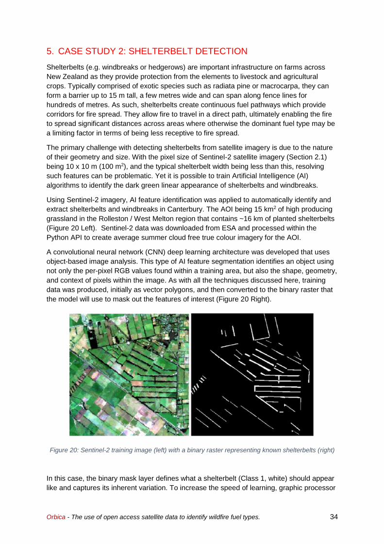
Using Sentinel-2 imagery, AI feature identification was applied to automatically identify and
extract shelterbelts and windbreaks in Canterbury. The AOI being 15 km2 of high producing
grassland in the Rolleston / West Melton region that contains ~16 km of planted shelterbelts
(Figure 20 Left). Sentinel-2 data was downloaded from ESA and processed within the
Python API to create average summer cloud free true colour imagery for the AOI.
A convolutional neural network (CNN) deep learning architecture was developed that uses
object-based image analysis. This type of AI feature segmentation identifies an object using
not only the per-pixel RGB values found within a training area, but also the shape, geometry,
and context of pixels within the image. As with all the techniques discussed here, training
data was produced, initially as vector polygons, and then converted to the binary raster that
the model will use to mask out the features of interest (Figure 20 Right).
Figure 20: Sentinel-2 training image (left) with a binary raster representing known shelterbelts (right)
In this case, the binary mask layer defines what a shelterbelt (Class 1, white) should appear
like and captures its inherent variation. To increase the speed of learning, graphic processor

Orbica - The use of open access satellite data to identify wildfire fuel types. 35
units (GPUs) were employed in parallel. By leveraging such hardware, processing speed is
an order of magnitude faster, but requires the imagery to be subdivided into smaller regions.
In this case the image was divided into patches of 128 X 128 pixels and then subdivided into
training and validation datasets. In total 12 patches were produced from a single training
image, and from this, nine patches were used to train the AI model and three patches were
ringfenced for validating model performance on different areas. Table 11 compares training
and validation results using several standard statistics used in assessing AI model
performance.
Table 11: Model accuracy and performance for shelterbelt detection
Training Patches
(128X128)
Validation Patches (128X128)
Number of images used 9 3
Time in minutes 15 1
Model loss (Error Rate %) 0.0015 0.0138
Jaccard Similarity Index
(IOU)
0.9345 0.8073
Pixel based accuracy 0.9994 0.9970
To assess model outputs, a CNN AI model was trained on a single AOI and then used to
predict shelterbelts on a new unknown area. Typically, to generate accurate high performing
models, approximately 10% of the total area to be predicted on would be provided as
correctly labelled training data. In this example, only a single tile of 16 km2 was used as an
input to the model, Figure 21 (left) showing the result of the trained model predicting
shelterbelts in a confined AOI while Figure 21 (right) displays a new area in which the AI has
not been exposed to, and thus completely untested. While the model output may appear to
resolve the features poorly, quality control checks show the model provides a 70% accuracy
in detecting shelterbelts in Canterbury Grasslands. Not a bad result when the extremely
limited amount of training data that was passed to the CNN model is considered.

Orbica - The use of open access satellite data to identify wildfire fuel types. 36
Figure 21: CNN model outputs. Training data (left) and testing/prediction (right)

Orbica - The use of open access satellite data to identify wildfire fuel types. 37
6. CASE STUDY 3: GORSE/BROOM SEASONAL IDENTIFICATION
Gorse (Ulex europaeus) and Broom (Cytisus scoparius) are two competitive weed species
that are similar in appearance, grow in the same environments and have a short
establishment period (Figure 22). Due to this fact, the two species have been combined in
LCDB. Although they appear similar, particularly at distance from the observer, both species
respond considerably differently to fire. Gorse is a significant contributor to fire risk due to its
ability to ignite fast and burn hot, having the potential to spread fire fast. It’s area of local
extent can also contribute to large areas of fire extent. This is particularly concerning in
summer when the winds are hot, and conditions are dry. Broom on the other hand is difficult
to burn and does not share the same fire behaviour characteristics of gorse. Because of this,
it is important to distinguish between the two in relation to wildfire management.
Two key differences between the species may aid in differentiation and allow the use of
satellite and aerial imagery to map their extent, particularly where a mix of species can be
found in one area.
• Physiology. Gorse flowers in bloom have more of an orange-yellow hue than
Broom, which has a brighter yellow colour. Although this may be a challenge
to the human eye, it is possible to train software to delineate between the two.
• Peak blooming time. Both species typically flower in spring and have separate
blooming times which occur over a window of a couple of weeks to one
month. The key challenge when delineating between Gorse and Broom from
satellite imagery is pinpointing the moment when one bloom ramps up and
the other winds down. Therefore, the winter flowering behaviour of Gorse is
particularly helpful to identify if the spring bloom contains gorse or whether it
is solely Broom.
Figure 22: Gorse orange-yellow bloom (left) and Broom bright yellow bloom (right)

Orbica - The use of open access satellite data to identify wildfire fuel types. 38
6.1. COLOUR DETECTION DELINEATION
Like exotic forestry, colour shifting using the Sentinel-Hub EO-Browser (Section 2.2.2) allows
greater variability in the display of different hues of yellow. This method has been
successfully applied to explore the temporal change in yellow flowers in an AOI in the hills
above Akaroa in Canterbury. Figure 23 shows a time sequence that shows the progression
from dark yellow on 3rd October through to bright yellow on 27th November. These images
show how the extent of yellow changes in conjunction with the shade of yellow supporting
the different blooming time of Gorse and Broom.
Figure 23: Yellow flower bloom over time
Assuming the blooming time of Broom in Canterbury to be November, a test was done
comparing areas identified by Environment Canterbury (ECan) (Figure 24) with Sentinel-2
imagery (Figure 25). The ECan features are mostly correct in their location when compared
with the bright yellow blooms in the satellite imagery.
Figure 24: Areas identified by ECan as being predominantly broom. Purple – dominant, Orange – common, Blue – frequent

Orbica - The use of open access satellite data to identify wildfire fuel types. 39
Figure 25: Sentinel-2 satellite imagery from 2019 showing a bright yellow bloom in mid-late November.
A further examination into the LCDB2 classification in relation to gorse has occurred in
Taupo (Figure 26), where a side-by-side comparison of the LCDB2 gorse classification and a
colour shifted satellite image from mid-late November 2017 was undertaken. It appears that
there is minimal crossover between the two, likely due to the difference in analysis times,
and that Gorse in this area is no longer correct. Additionally, depending on the acquisition
date of imagery that was used to create LCDB2, it also may not be Gorse. As shown in the
Canterbury examples above, Broom also flowers in mid-late November and has a similar
bright yellow flower to Gorse.
Figure 26: LCDB2 classified gorse and broom in yellow (left), Satellite imagery (November 2017) showing yellow bloom (right)

Orbica - The use of open access satellite data to identify wildfire fuel types. 40
6.2. TEMPORAL DETECTION DELINEATION
Given that Gorse and Broom have similar coloured flowers, this may cause difficulties when
attempting to delineate between the two in a mixed species setting. The use of a single date
imagery source, even one of high resolution (i.e. Worldview 3), may not be adequate in
providing an AI algorithm a chance to successfully identify a feature/species of choice. Given
that the Sentinel-2 imagery used in this report is of medium spatial (i.e. 10 m/px), but
relatively high temporal resolution (five-day revisit time), a different approach may be
needed.
Such an alternative to finding the colour difference between blooms is to employ the
temporal component of flowering to determine if Gorse is present. Thus, extending the time
component from a couple of weeks to several months may increase the probability of
separating Gorse from Broom.
The blooming period for Gorse is generally longer and earlier to that of Broom, typically
beginning in mid-late winter and extending through spring and summer. In contrast, Broom
tends to only flower during mid-late spring. Although the winter bloom of Gorse may be less
dramatic than the spring bloom, it is still possible to detect its presence (Figure 27).
Figure 27: Gorse bloom in winter (left) and spring (right). Note that these images have a different colour setting than those in Figure 23.
To employ such a method would require image processing software and a customised
yellow spectrum. Additionally, it would also take a month, or at least two weeks of images to
determine if gorse or broom is present and the degree of change in the coverage. It would
also be possible to determine the degree of change of average colour of each pixel to help
detect the period where the bloom goes from an orange yellow to a brighter yellow to assist
with species delineation.
An example of this application would be if yellow is present only in November, its likely to be
broom. But if yellow present from late August to late November, its likely gorse is present.
The colour change analysis could assist in delineating where gorse and broom are present.
Unfortunately, given that building custom colour stretches, waiting for the correct period and
the number of images required is particularly time intensive, therefore it may only be
financially viable to undertake this once a year.

Orbica - The use of open access satellite data to identify wildfire fuel types. 41
6.3. IMAGE CLASSIFICATION
To apply a machine learning methodology to the problem of Gorse/Broom detection and
delineation, an AOI was chosen in the hills on either side of Akaroa Harbour. Sentinel-2 true
colour imagery was collected for the period October to November where a clear shift in the
extent of yellow vegetation was observed. The open-source image processing application
Fiji (https://imagej.net/Fiji), was used to build a training dataset for the earlier part of the
Gorse blooming period (Early October) and applied to a second time-slice in which Broom
was likely to be flowering (November).
The Sentinel-2 true colour imagery for the October 2017 period (Figure 28) shows Gorse as
having a subdued orange/yellow colour and typically being restricted to the higher elevation
ridgetops and their associated slopes. In contrast, in the November imagery (Figure 29), the
same vegetation appears far brighter and has a smaller extent. While this is likely due to the
differing blooming periods and species composition between the Gorse and Broom, it may
also be related to hue and gamma differences between the two images.
Figure 28: Sentinel-2 imagery from October 2017.
Figure 29: Sentinel-2 imagery from November 2017.
Using the Fiji software, key areas from the above imagery were extracted for use as training
data. The classified results for each date were post processed to reduce any classification
noise and are shown in Figures 30 and 31.

Orbica - The use of open access satellite data to identify wildfire fuel types. 42
Figure 30: Gorse areas identified in October imagery using the Fiji classifier.
Figure 31: Gorse areas identified in November imagery using the Fiji classifier.
We have shown that by using a range of techniques the separation of Gorse vs Broom is
possible using Sentinel-2 data. Even with its lower resolution, the short revisit time of the
satellites allows the temporal nature of blooming times between the two species to be
quantified.

Orbica - The use of open access satellite data to identify wildfire fuel types. 43
7. CASE STUDY 4: URBAN EXPANSION
A key part of assessing the threat that wildfire poses to people and property is understanding
the expansion of urban or peri-urban areas into the surrounding rural area. With changes to
city limits and shifting population centres, the potential for proximity of residential and
commercial properties to extensive areas of vegetation has increased. This is especially
important when considering the risk posed by shelterbelts and windbreaks, commonly found
in farm settings, as a fire corridor though the establishment of a continuous fuel pathway.
Given these concerns, developing a methodology to enhance LCDB5, which is based on
2018 data, will provide a clearer picture of potential risk to properties along the rural-urban
interface.
To examine the changes in urban and commercial expansion, Sentinel-2 imagery was
obtained for January 2016 and 2020. Christchurch was chosen due to its extreme post-
earthquake population shift, in which residents in the affected Eastern and Central suburbs
have relocated to Western and Northern areas.
Imagery was created using the red and SWIRs band:
𝐹𝐶𝑆𝑊𝐼𝑅 = 𝑅(𝐵12) 𝐺(𝐵11) 𝐵(𝐵4)
Where Red = SWIR2 (Band 12), Green = SWIR 1 (Band 11) and Blue = Red (Band 4). The
use of such a false colour band combination highlights the differences between the urban
and rural areas between the two years (Figure 32).
Figure 32: Sentinel-2 false imagery for Christchurch city in 2016 (Left) and 2020 (Right).
An initial observation of the imagery shows the city as being comprised of two distinct pixel
textures and colours.
• Type 1. Light pixels. Located in regions with a high proportion of larger
industrial and commercial warehouses and buildings. The large roofs,

Orbica - The use of open access satellite data to identify wildfire fuel types. 44
typically galvanised or painted white, provide a highly reflective surface to all
wavelengths. The central commercial corridor running east / west across the
city is particularly obvious in Figure 32.
• Type 2. Grey pixels. These represent the highest proportion of the city and
are caused by a mosaic of residential dwellings and their associated gardens.
Compared to that of the commercial zone, the different spectral responses
from a range of vegetation, roof size and building material produce a more
textured appearance in the imagery. Additionally, due to the smaller size of
residential building compared to the 10 m pixel size resolved by the Sentinel-
2 imagery, the reflected wavelengths are a mix of building and vegetation.
Using the false colour imagery, a relatively small number of areas (n=15) representing the
above two types were digitised and provided to a Support Vector Machines (SVM)
classification algorithm as training data. As the identification of urban areas is a binary
problem (absence vs presence), the training data only needed to represent the variation
observed.
SVM excels in binary segmentation and thus the relatively simple set of input pixel types and
limited training data have produced the outputs shown in Figure 33.
Figure 33: Urban areas in 2016 (Left) and 2020 (Right) from the SVM model.
Unsurprisingly the model shows an expansion of areas now classed as urban into the
western formally rural areas, particularly around the towns of Rolleston, West Melton, and
Lincoln. Both commercial/industrial and residential areas have been well segmented from
the surrounding rural and peri-rural area. If the difference between the 2016 and 2020 data
is calculated, the result is the areas of absolute change (Figure 34). Unfortunately, as can be
seen, some areas of non-urban areas have been highlighted (i.e. wastewater ponds to the
east).
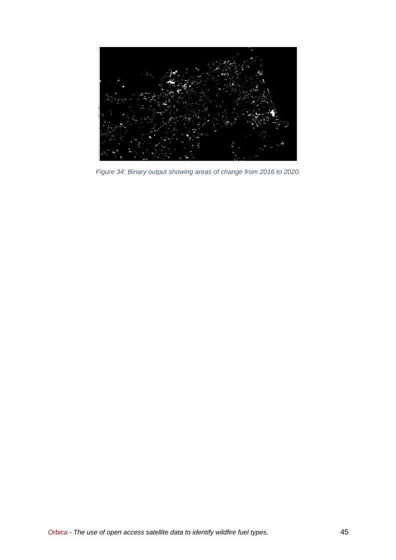
Orbica - The use of open access satellite data to identify wildfire fuel types. 45
Figure 34: Binary output showing areas of change from 2016 to 2020.

Orbica - The use of open access satellite data to identify wildfire fuel types. 46
8. CASE STUDY 5: WATER BODY DETECTION
While obviously not a wildfire fuel source, water availability is a key resource when
considering rural fire operations in remote locations. This is especially pertinent to helicopter
operations that use monsoon buckets and require access to open water bodies during
wildfire outbreaks. Therefore, identifying and providing an up-to date dataset of suitable
locations to collect or extract water is a key component of any wildfire response database.
To explore the AI detection of water features, an AOI was defined that covered
approximately a quarter of the Canterbury region. Within this area were located a range of
surface water types such as lakes, ponds, reservoirs, lagoons, and rivers, all of which play
an important role in wildfire management either as a water resource or a physical barrier to
fire spread. To assess the use of AI in water detection 10 m resolution Sentinel-2 true-colour
imagery was acquired from January 2016 to June 2019 and filtered to ensure less than 10%
cloud cover (Figure 35).
Figure 35: Sentinel-2 imagery used in the Canterbury region to assess water coverage.
Additionally, to generate the required training data, the 2018 LINZ water body dataset was
used to define areas of surface water.
Using the Sentinel-2 imagery, a relatively standard band combination was used to enhance
the detection of surface water, that being the Normalised Difference Wetness Index (NDWI)
which is derived from the relative differences between the green (Band 3) and near infrared
(Band 8).
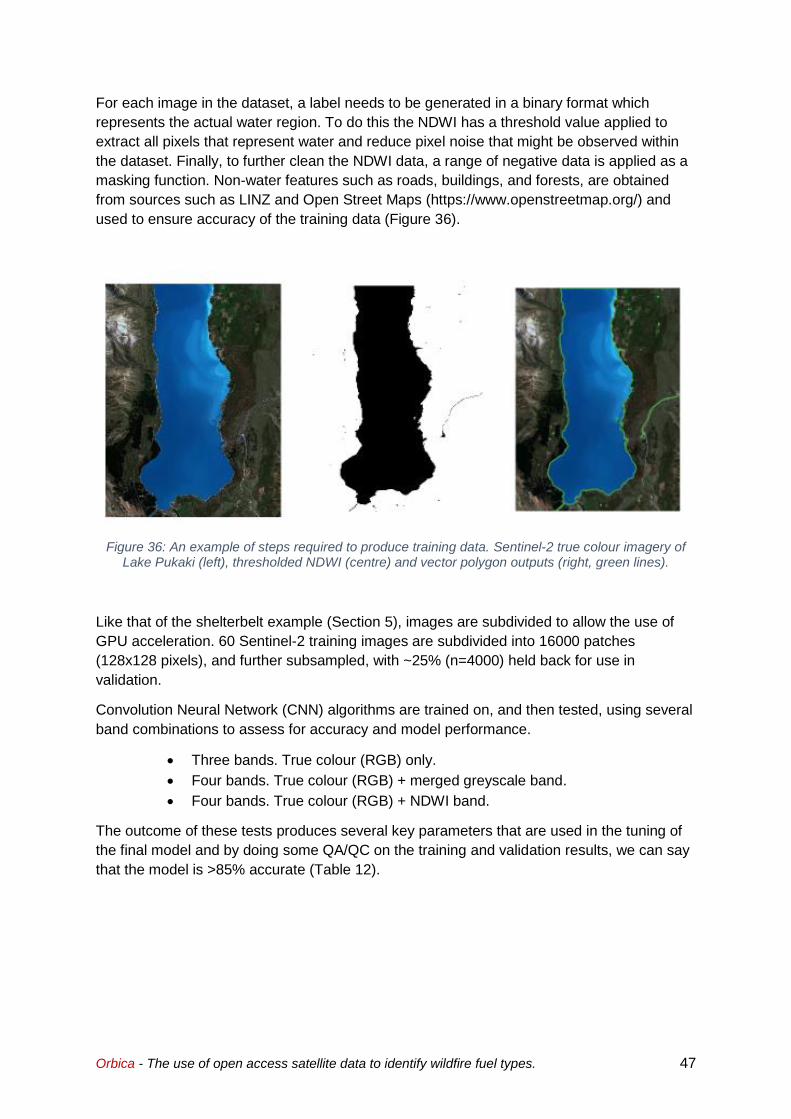
Orbica - The use of open access satellite data to identify wildfire fuel types. 47
For each image in the dataset, a label needs to be generated in a binary format which
represents the actual water region. To do this the NDWI has a threshold value applied to
extract all pixels that represent water and reduce pixel noise that might be observed within
the dataset. Finally, to further clean the NDWI data, a range of negative data is applied as a
masking function. Non-water features such as roads, buildings, and forests, are obtained
from sources such as LINZ and Open Street Maps (https://www.openstreetmap.org/) and
used to ensure accuracy of the training data (Figure 36).
Figure 36: An example of steps required to produce training data. Sentinel-2 true colour imagery of Lake Pukaki (left), thresholded NDWI (centre) and vector polygon outputs (right, green lines).
Like that of the shelterbelt example (Section 5), images are subdivided to allow the use of
GPU acceleration. 60 Sentinel-2 training images are subdivided into 16000 patches
(128x128 pixels), and further subsampled, with ~25% (n=4000) held back for use in
validation.
Convolution Neural Network (CNN) algorithms are trained on, and then tested, using several
band combinations to assess for accuracy and model performance.
• Three bands. True colour (RGB) only.
• Four bands. True colour (RGB) + merged greyscale band.
• Four bands. True colour (RGB) + NDWI band.
The outcome of these tests produces several key parameters that are used in the tuning of
the final model and by doing some QA/QC on the training and validation results, we can say
that the model is >85% accurate (Table 12).

Orbica - The use of open access satellite data to identify wildfire fuel types. 48
Table 12: Typical output of CNN training vs validation vs testing model.
Final model outputs for the unknown testing areas are shown for lakes (Figure 37), braided
rivers (Figure 38) and a mixture of water body types including alpine tarns and ponds (Figure
39).
Figure 37: Sentinel-2 true colour imagery (left) and the AI outputs (right) for Lake Ohau in South Canterbury. Note the lack of definition between lakes Middleton and Ohau (green box) likely due to
incomplete classification in the AI processing pipeline.
Training Validation Testing
Number of arrays 12066 4021 2681
Number of images 45 15 10
Model loss (%) 0.0098 0.0090 -
Jaccard similarity (IOU) 0.8988 0.9022 -
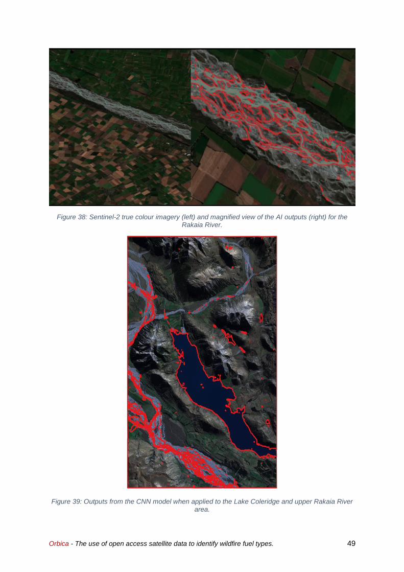
Orbica - The use of open access satellite data to identify wildfire fuel types. 49
Figure 38: Sentinel-2 true colour imagery (left) and magnified view of the AI outputs (right) for the Rakaia River.
Figure 39: Outputs from the CNN model when applied to the Lake Coleridge and upper Rakaia River area.

Orbica - The use of open access satellite data to identify wildfire fuel types. 50
Results from this example show that the combination of CNN machine learning, and
multispectral Sentinel-2 imagery can be used to extract areas of surface water with a fairly
high level of accuracy. As always in small case study investigations like this example,
additional steps could be added to increase accuracy and processing speed, while
decreasing model error. In particular:
• More training data.
• Tuning of Hyperparameters to increase the model accuracy.
• The addition of new imagery like thermal (Landsat 8) and other spectral
bands (Sentinel-2) will increase the amount of input data pixels provided to
the model and thus will help deep learning models to identify new features.
• Adding more post processing to filter/remove noise from output predictions.
• Investigate methods to improve class imbalances (i.e. the ratio between water
and non-water pixels).
Orbica - The use of open access satellite data to identify wildfire fuel types. 51
9. CONCLUSION
The findings presented in this report show, albeit at a relatively basic level, that the use of
machine learning and artificial intelligence algorithms can be used to identify and isolate key
wildfire fuel types. As well as a deep dive on the class differences between LCDBv2 and v5,
our results find:
• The systematic errors observed between previous and current versions of
LCDB may make the use of future releases problematic for the differentiation
of wildfire fuel classes and associated fire behaviour modelling.
• That given the correct amount and type of training data, machine-learning and
artificial intelligence models can be used to detect a range of expanded-fuel
classes, not current in LCDB5 and certainly not in LCDB2.
• Sentinel-2 at 10 m/px provides an adequate spatial resolution for most
purposes. Only shelterbelts with a width less than 10 m may be problematic.
• Using colour and temporal shifting techniques, gorse and broom may be able
to be separated at some level using their differing flower colour and blooming
times.
• Using aerial imagery, several exotic forestry classes can be identified.
o Cleared areas (i.e. slash and cutover).
o Different age classes.
• Changes can be relatively easy to observe using several Sentinel-2 products.
In cases where this is not possible, applying colour shifting techniques may
increase the accuracy in the identification of native vs exotic forestry stands.
• False colour imagery provides a solid platform for the detection of urban
areas and thus the encroachment into rural areas.
• Sentinel-2 NDWI data can be used to identify water features such as lakes
and rivers throughout Canterbury.
9.1. FUTURE RESEARCH DIRECTIONS
Given that this research only touches on a limited number of fuel types, several areas where
expanded work may be a benefit have been recognised.
• More targeted work on fuel types. While good progress was made on
recognising the extent of gorse vs broom, other mixed fuel types would also
benefit from a closer view.
• Grasslands. New Zealand has a variety of grass types, from dry alpine
tussocks and wet marshlands. Currently most of these differing fuel types are
clustered together into the ubiquitous LCDB “Grasslands” class which poses
problems for determining fire behaviour. The identification of grassland extent
and species is also important when considering the encroachment of urban
areas.
• Exotic vs native forestry. While the identification of exotic plantations was
covered at a simple level, a more in-depth investigation would allow the
development of a more robust AI model. If more forestry companies could
Orbica - The use of open access satellite data to identify wildfire fuel types. 52
supply GIS data for the extent and species of plantations, this could be used
as training data to drive a far more accurate model using satellite imagery.
• Testing. Producing a small AOI with the AI generated features from this
project and integrating them into LCDB5.
• Full AI model. For this work, the discussed fuel types were treated as their
own discrete entity, each having a range of imagery, processing, and
algorithm types. Yet this is not the case as all these fuel types are a
patchwork across the New Zealand landscape. Now with our understanding
of how machine learning, and AI models react to the training data and the
requirements needed to produce more accurate models, a proof-of-concept
methodology using a single multiclassification AI model could be developed.
This work could be done with a local view, being run on inhouse machines, or
the initial start of a cloud-based solution (see below).
9.2. IMPLEMENTATION
Given the final option presented above, such an AI driven classification pipeline could be
imagined in several ways, depending on the required timeliness of data delivery and update
frequency. While estimated costs have been added, final costing may vary considerably
based on the extent of the AOI being processed (All prices in NZD).
▪ Timed release. In this scenario FENZ would subcontract the production of an
augmented LCDB that adds/updates key vegetation fuel types as specified.
This would be produced on local machines and would not require any cloud-
based technologies (i.e. AWS and Azure). This dataset would not be the
latest snapshot of vegetation fuel types but be far more accurate than the
currently employed version of LCDB. The frequency of releases could be
biannually or annually as required.
Estimated cost per release: $20-40k.
▪ On demand (ad-hoc) – local computing. A reactive approach would be that a
targeted dataset, using an AOI defined by an active event, is produced when
required. An advantage is that the latest imagery can be used and thus the
dataset is the most update (within the five-day revisit time of Sentinel-2). This
could also be combined with high resolution commercial imagery if required.
Estimated cost per event: $5-15K.
▪ On demand – cloud computing. Like the above, but the entire process is
based within a cloud-based infrastructure. In this situation, FENZ could have
complete control of the process and outputs would be automatically
generated on a weekly basis, or manually requested in the event of an active
wildfire. This is a proactive approach where the latest data is constantly being
produced.
Estimated cost for development and setup: $100-200k.

Orbica - The use of open access satellite data to identify wildfire fuel types. 53
For all these scenarios, a web portal for operational and management purposes using this
data can also be produced. The ability to provide “boots on the ground” firefighting personnel
with mobile accessible data may be a powerful tool in the fight against wildfires.