the two margin problem in insurance markets
TRANSCRIPT

The Two Margin Problem in Insurance Markets∗
Michael Geruso† Timothy J. Layton‡ Grace McCormack§ Mark Shepard¶
September 24, 2019
Abstract
Insurance markets often feature consumer sorting along both an extensive margin (whether tobuy) and an intensive margin (which plan to buy). We present a new graphical theoretical frame-work that extends a workhorse model to incorporate both selection margins simultaneously. Akey insight from our framework is that policies aimed at addressing one margin of selection ofteninvolve an economically meaningful trade-off on the other margin in terms of prices, enrollment,and welfare. Using data from Massachusetts, we illustrate these trade-offs in an empirical suffi-cient statistics approach that is tightly linked to the graphical framework we develop.
∗We thank Sebastian Fleitas, Bentley MacLeod, Maria Polyakova and Ashley Swanson for serving as discussants forthis paper. We also thank Kate Bundorf, Marika Cabral, Amitabh Chandra, Vilsa Curto, Leemore Dafny, Keith Ericson,Amy Finkelstein, Jon Gruber, Tom McGuire, Neale Mahoney, Joe Newhouse, Evan Saltzman, Brad Shapiro, Pietro Tebaldi,and participants at NBER Health Care, NBER Insurance Working Group, CEPRA/NBER Workshop on Aging and Health,the 2019 Becker Friedman Institute Health Economics Initiative Annual Conference at the University of Chicago, the 2019American Economic Association meetings, the 2018 American Society of Health Economists meeting, the 2018 AnnualHealth Economics Conference, the 2018 Chicago Booth Junior Health Economics Summit, and seminars at the BrookingsInstitution and the University of Wisconsin for useful feedback. We gratefully acknowledge financial support for thisproject from the Laura and John Arnold Foundation, the Eunice Kennedy Shriver National Institute of Child Health andHuman Development center grant P2CHD042849 awarded to the Population Research Center at UT-Austin, the Agency forHealthcare Research and Quality (K01-HS25786-01), and the National Institute on Aging, Grant Number T32-AG000186.No party had the right to review this paper prior to its circulation.†University of Texas at Austin and NBER. Email: [email protected]‡Harvard University and NBER. Email: [email protected]§Harvard University. Email: [email protected]¶Harvard University and NBER. Email: [email protected]

1 Introduction
Some of the most important problems in health insurance markets stem from adverse selection, or the
tendency of sicker consumers to exhibit higher demand for insurance. Concerns about adverse selec-
tion have motivated a variety of regulatory interventions in the U.S. and around the world, including
insurance mandates, penalties for being uninsured, subsidies for purchasing insurance, risk adjust-
ment transfers, benefit regulation, and reinsurance. Policy discussions about how to address adverse
selection have become salient in the U.S. as many public programs have shifted toward providing
health insurance via regulated markets (Gruber, 2017).
But, a deeper look reveals that not all policies combating adverse selection are targeted at the
same problem. Policies such as mandates and subsidies combat selection on the extensive margin (or
“against the market”). This type of selection is characterized by sicker people being more likely to
buy insurance. It leads to higher insurer costs and higher consumer prices and causes some healthy
people to opt out. Policies such as risk adjustment and benefit regulation, on the other hand, combat
selection on the intensive margin (or “within the market”). This type of selection is characterized
by sicker people being more likely to purchase more generous plans within the market. Intensive
margin selection drives up the price of generous plans relative to skimpy ones and results in too
many consumers choosing skimpy plans. In some cases, selection within the market may be so strong
that generous contracts cannot be sustained, and the market for them unravels entirely (Cutler and
Reber, 1998).
Prior work has recognized these two problems and has studied policies targeted at each. How-
ever, this literature has largely considered these two forms of selection in isolation—either assuming
all consumers buy insurance and focusing on the intensive margin (e.g., Handel, Hendel and Whin-
ston, 2015), or assuming all contracts within the market are identical and focusing on the extensive
margin (e.g., Hackmann, Kolstad and Kowalski, 2015). By ignoring one margin or the other, the selec-
tion problem is usefully simplified. In empirical work, it becomes amenable to a sufficient statistics
approach based on demand and cost curves defined in reference to a single price—either the price
of insurance or the price difference between a generous vs. a skimpy plan (Einav, Finkelstein and
Cullen, 2010). However, this simplification does not allow for potential interactions between these
two margins of selection.
In this paper, we generalize the canonical insurance market framework to address both margins
1
simultaneously. The benefit of doing so is not merely a technical curiosity. It has first-order pol-
icy importance in settings like the ACA Marketplaces where both the generosity of coverage and
rates of uninsurance are serious concerns. To see why, consider an insurance mandate—a policy that
aims to correct extensive margin selection by bringing healthy marginal consumers into the market.
Our framework shows how a mandate that succeeds in increasing rates of insurance coverage will
likely worsen selection on the intensive margin. Intuitively, the mandate brings more healthy/low-
cost consumers into the market. Because these new consumers tend to select the lower-price (and
lower-quality) plans, the risk pools of those plans will get even healthier. In equilibrium, these plans
will further reduce prices, siphoning additional consumers away from higher-quality plans on the
intensive margin, causing prices for high-quality coverage to spiral upwards. These two offsetting
effects (improving take-up and inducing within-market unraveling) represent a clear example of the
intensive/extensive margin interactions that are the focus of our paper. Recent theoretical insights
from Azevedo and Gottlieb (2017), as well as empirical findings from Saltzman (2017) indicate that
this is an important omission in contexts like the ACA Marketplaces, where both margins of selection
matter. In practice, we show that the size of such effects are first-order in terms of plan choices and
welfare.
One of our main contributions is to provide a graphical demand-cost framework that lets economists
visualize (and teach) the two-margin selection problem in a transparent way. To do so, we build on
the influential work of Einav, Finkelstein and Cullen (2010) and Einav and Finkelstein (2011), who
show how to visualize selection markets in terms of demand, average cost, and marginal cost curves.
We generalize their model to allow for two vertically ranked plans—a more generous H plan and
a less generous L plan—plus an outside option of uninsurance (U). Although stylized, this verti-
cal model captures the core intuition of the two selection margins: an intensive margin difference
in generosity (H vs. L) and an extensive margin option to exit the market (by choosing U). It also
captures the key feature of adverse selection: that higher-risk consumers have greater willingness to
pay for generous coverage—both for H relative to L, and for L relative to U. Our vertical model is
the simplest framework that captures these features, and is useful for developing intuition around
a potentially multi-dimensional problem by allowing the market to be represented in standard two-
dimensional graphs with familiar demand and cost curves. Equilibrium prices, market shares, and
social surplus can all be easily visualized.
2

As in Einav, Finkelstein and Cullen (2010), there is a tight link between our model and the estima-
tion of sufficient statistics used to characterize equilibrium and welfare. Econometric identification is
analogous, though exogenous price variation along two margins is required—for example, indepen-
dent variation in the price of a skimpy plan and in the price of a generous plan.1
After developing the graphical framework, we use it to show how policies and regulatory ac-
tions that counteract selection on one margin can interact with the other. The relevance of these
“cross-margin” interactions is the key conceptual take-away of our paper. We show that a mandate’s
impact on plan generosity is, in fact, an instance of a broader phenomenon that encapsulates many
relevant policy interventions currently in place in insurance markets. These include plan benefits
requirements, network adequacy rules, risk adjustment, reinsurance, subsidies, and behavioral in-
terventions like plan choice architectures or auto-enrollment. Each involves a potential trade-off.
Policies that aim to address intensive margin selection tend to worsen extensive margin selection,
and vice-versa.
The graphical model helps show why these cross-margin interactions occur. The key insight is
that for each plan, either its demand or average cost curve is not a price-invariant model primitive
(as is true in a two-option model) but an equilibrium object that depends on the other plan’s price.
Policies that target one selection margin typically influence market prices (e.g., the mandate lowers
PL relative to PH), which in turn shifts demand or cost curves that determine the other margin (e.g.,
the lower PL reduces demand for H). This cross-plan dependence of demand and average costs is
the key missing piece when the two margins are analyzed separately. We show how the geometry
of the demand/cost curves generates this dependence and lets analysts think about cross-margin
interactions in a structured way.
With the intuition and price theory in place, we analyze the model’s insights empirically us-
ing demand and cost estimates from Massachusetts’ CommCare program, a precursor to the state’s
ACA health insurance Marketplace. CommCare was introduced in 2006 to provide subsidized health
insurance coverage to low-income residents who did not qualify for Medicaid. In this setting, Finkel-
stein, Hendren and Shepard (2019) document significant adverse selection both into the market and
within the market between a narrow-network, lower-quality option and a set of wider-network,
higher-quality plans. In a regression discontinuity design that exploits discontinuities in the income-
1Or alternatively, variation in a market-wide subsidy for selecting any plan and independent variation in the pricedifference between bare bones and generous plans.
3
based premium subsidy scheme, they construct demand and cost curves for the lower and higher
quality plans. We use these demand and cost curves in a number of counterfactual exercises that sim-
ulate equilibrium as we vary benefit design rules, mandate penalties, and risk adjustment strength.
The empirical exercise, beyond demonstrating how our framework can be used, generates sev-
eral policy insights. The size of the unintended cross margin effects can be large enough to imply
significant impacts on market shares. We find that a strong mandate sufficient to move all consumers
into insurance—increasing enrollment by around 25 percentage points in our setting—can cause the
market share of more generous plans to shrink by more than 15 percentage points, or 35% of base-
line market share. In the other direction, strengthening risk adjustment transfers to the point where
the market “upravels” to include only generous coverage can substantially reduce market-level con-
sumer participation—in our setting by as much as 15 percentage points or 60% of the baseline unin-
surance rate. With the additional assumption that consumer choices reveal plan valuations, we find
that the cross-margin welfare impacts can be similarly large (and often first-order), under a range of
parameters describing the external social cost of remaining uninsured.
Further, we show that in some settings, cross-margin interactions are critical for determining op-
timal policy. When intensive margin policies (such as risk adjustment) are weak, it can be optimal
to also have weak extensive margin policies (such as an uninsurance penalty). But when intensive
margin policies are strong, on the other hand, it can be optimal to also have strong extensive mar-
gin policies. These results show that in these markets, regulators are operating in a world of the
second-best and must consider interactions between the two margins of selection in order to de-
termine constrained optimal policy. This is true whether optimality is viewed from a formal social
surplus perspective or reflects a political preference over rates of insurance coverage on the one hand
and insurance quality on the other.
Our paper contributes to a growing literature on adverse selection in health insurance markets.
Our main contribution is to provide a graphical model that unites the two key strands of this lit-
erature that were previously somewhat disconnected. The first strand focuses on extensive margin
selection and stems from the seminal work of Akerlof (1970), with more recent theoretical advances
by Hendren (2013), Hendren (2018), and Mahoney and Weyl (2017) and empirical applications by
Einav, Finkelstein and Cullen (2010), Bundorf, Levin and Mahoney (2012), Hackmann, Kolstad and
Kowalski (2015), Tebaldi (2017), Einav, Finkelstein and Tebaldi (2018) and others. The second strand
4

focuses on intensive margin selection, studying sorting across fixed contracts within the market (Han-
del, Hendel and Whinston, 2015; Shepard, 2016) as well as papers that study the effects of intensive
margin selection on the contracts insurers offer (Glazer and McGuire, 2000; Veiga and Weyl, 2016;
Carey, 2017; Lavetti and Simon, 2018; Geruso, Layton and Prinz, 2019). The most directly connected
work is a prior theoretical contribution by Azevedo and Gottlieb (2017) that points out the potential
cross-margin effects of a mandate, and a complementary analysis (concurrent with ours) by Saltzman
(2017) that investigates cross margin effects using a structural model.
Our insights about cross-margin interactions are relevant for active policy debates in the ACA
and other insurance settings. For example, recently states have been given increasing flexibility to
weaken ACA Essential Health Benefits or risk adjustment transfers (intensive margin policies)—with
the stated goal being to lower plan prices and reduce uninsurance (a cross-margin effect). On the
other hand, state efforts to simplify enrollment (Domurat, Menashe and Yin, 2018), auto-enroll certain
consumers (Shepard, 2019), or enact mandate penalties (all extensive margin policies) may create
unintended consequences on the intensive margin. More broadly, our model is also relevant to other
settings with two selection margins, including the Medicare program (with its Medicare Advantage
option), employer programs with a plan choice decision and a participation decision (e.g., CalPERS),
national health insurance systems with an opt-out (e.g., Germany), other insurance markets such as
auto insurance and long-term care insurance where both the intensive and extensive margins may
be important, and other non-insurance markets like consumer credit where there is evidence of both
extensive and intensive margin risk selection (Adams, Einav and Levin, 2009; Einav, Jenkins and
Levin, 2012).
The rest of the paper is organized as follows. Section 2 presents the graphical vertical model.
Section 3 applies the model to show two-margin impacts of various policies. Sections 4-6 apply the
model with simulations: section 4 discusses methods; section 5 shows price and enrollment results;
and section 6 shows welfare results. Section 7 concludes.
2 Model
Our goal in this section is to develop a theoretical and graphical model that depicts insurance market
equilibrium and welfare in the spirit of Einav, Finkelstein and Cullen (2010) (“EFC”), while allowing
for the possibility that interventions affecting selection on one margin may affect selection on another.
5
This requires an insurance plan choice set with at least three options. Consider two fixed contracts,
j = {H, L}, where H is more generous than L on some metric, and an outside option, U. In the focal
application of our model to the ACA’s individual markets, U represents uninsurance.
Each plan j ∈ {H, L} sets a single community-rated price Pj that (along with any risk adjustment
transfers—see below) must cover its costs. Consumers make choices based on these prices and on
the price of the outside option, PU = M.2 In our focal example, M is a mandate penalty. The dis-
tinguishing feature of U is that its price is exogenously determined; it does not adjust based on the
consumers who select into it. This is natural for the case where U is uninsurance or a public plan like
Traditional Medicare. P = {PH, PL, PU} is the vector of prices in the market.
In the most general formulation, demand in this market cannot be easily depicted in two-dimensional
figures. To make the cross-margin effects of interest clearer, we impose a vertical model of demand,
which assumes contracts are identically preference-ranked across consumers. Although the strict ver-
tical assumption is not necessary for many of our main insights to hold, it captures the key features of
the issues raised by simultaneous selection on two margins in a simple way that allows for graphical
representation. In the next subsections, we present the vertical model, then add the cost curves, and
finally show how to find equilibrium and welfare. In the appendix, we discuss the implications of
relaxing the vertical demand assumption.
2.1 Demand
The model’s demand primitives are consumers’ willingness-to-pay (WTP) for each plan. Let Wi,H be
WTP of consumer i for plan H, and Wi,L be WTP for L, both defined as WTP relative to U (Wi,U ≡ 0).
We make the following two assumptions on demand:
Assumption 1. Vertical ranking: Wi,H > Wi,L for all i
Assumption 2. Single dimension of WTP heterogeneity: There is a single index s ∼ U[0, 1] that orders
consumers based on declining WTP, such that W ′L(s) < 0 and W ′H(s)−W ′L(s) < 0 for all s.
These assumptions, which are a slight generalization of the textbook vertical model,3 involve
2Below, we allow that consumers may receive a subsidy, S, so that choices are based on post-subsidy prices, Pconsj =
Pj − S.3Our vertical model follows the format of Finkelstein, Hendren and Shepard (2019). It is a generalization of the textbook
vertical model in which products differ on quality (Qj) and consumers differ on taste for quality (βi), so that WTP equals:Wi,j = βiQj and utility equals Ui,j = Wi,j − Pj = βiQj − Pj.
6
two substantive restrictions on the nature of demand. First, the products are vertically ranked: all
consumers would choose H over L if their prices were equal. This is a statement about the type of
setting to which our model applies. The vertical model applies best when plan rankings are clear—
e.g., a low- vs. high-deductible plan, or a narrow vs. complete provider network plan. Importantly,
these are precisely the settings where intensive margin risk selection is most relevant. When plans
are horizontally differentiated (such as in the Covered California market; see Tebaldi, 2017, Saltzman,
2017, Einav, Finkelstein and Tebaldi, 2018), it is less likely that high-risk consumers will heavily select
into a single plan or type of plan. In such cases, the existing EFC framework can capture the main way
risk selection matters: in vs. out of the market (the extensive margin). Our model is designed to study
the additional issues that arise when both intensive and extensive margins matter simultaneously.
Even in settings without apparent vertical differentiation across plans within the market, our model
can be useful in assessing counterfactual policies that might generate this type of differentiation. In
particular, our examples below imply that a regulator encouraging vertically differentiated entrants
may generate unintended cross-margin effects on the rates of uninsurance.4
Second, consumers’ WTP for H and L—which in general could vary arbitrarily over two dimensions—
are assumed to collapse to a single-dimensional index, s ∈ [0, 1]. Higher s types have both lower WL
and a smaller gap between WH and WL. Lower s types both care more about having insurance (L
vs. U) and more about the generosity of coverage (H vs. L). This assumption is natural in many
cases; indeed it holds exactly in a model where plans differ purely in their coinsurance rate (see, e.g.,
Azevedo and Gottlieb, 2017). Substantively, Assumption 2 restricts consumer sorting and substitution
patterns among options when prices change. The primary consequence of this assumption is that con-
sumers are only on the margin between adjacent-generosity options–between H and L or between L
and U. No consumer is on the margin between H and U, so if the price of U (the mandate penalty)
increases modestly, the newly insured all buy L (the cheaper plan), not H. This restriction captures
in a strong way the general (and testable) idea that these are the main ways consumers substitute in
response to price changes. With this restriction in place (and under a price vector at which all op-
tions are chosen), consumers sort into plans with the highest-WTP types choosing H, intermediate
types choosing L, and low types choosing U. We show that weakening this assumption—allowing an
4Further, an apparent lack of vertical differentiation in a market may itself be an equilibrium outcome reflecting forcesthat our vertical model captures. For example, a market for generous coverage may have already unraveled due to cross-margin effects, leaving only lower-quality, horizontally differentiated plans.
7

Figure 1: Demand and Consumer Sorting under Vertical Model
$ WH(s)
WL(s)
PL
Buy L Uninsured
DH(s;PL)
PH
Buy H
Demand curve for H (given PL) DH = WH(s) – WL(s) + PL
Demand curve for any insurance (H or L) = WL(s)
Intensive margin Extensive margin
s
Consumer WTP type
=∆P
Notes: The graph shows demand and consumer sorting under the vertical model. WH(s) and WL(s) are willingness to payfor the H and L plans. DH(s; PL) is the demand curve for H (as a function of PH), which depends on the value of PL. Seethe body text for additional description.
H-U margin—does not change the key implications of the model as long as most consumers exhibit
vertical preferences (see Appendix A).
Figure 1 plots a simple linear example of WH(s) and WL(s) curves that satisfy these assumptions.
The x-axis is the WTP index s, so WTP declines from left to right as usual. Let sLU(P) be the extensive-
marginal type who is indifferent between L and U at a given set of prices P. Assuming for now that
PU ≡ M = 0, this cutoff type is defined by the intersection of L’s WTP curve WL and L’s price:
WL (sLU) = PL. (1)
Consumers to the right of sLU go uninsured. Those to the left buy insurance. Therefore, WL(s)
represents the (inverse) demand curve for any formal insurance (H or L). 5
5In the more general case where consumers receive subsidies for purchasing insurance or pay a penalty when choosingU, WL(s) and the (inverse) demand curve for insurance will diverge. Specifically, DL(s) = WL(s) + S + M. For simplicity,
8
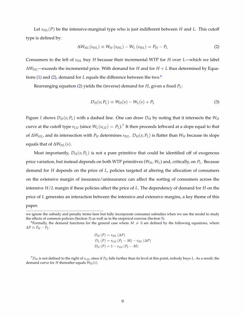
Let sHL(P) be the intensive-marginal type who is just indifferent between H and L. This cutoff
type is defined by:
∆WHL(sHL) ≡WH (sHL)−WL (sHL) = PH − PL (2)
Consumers to the left of sHL buy H because their incremental WTP for H over L—which we label
∆WHL—exceeds the incremental price. With demand for H and for H + L thus determined by Equa-
tions (1) and (2), demand for L equals the difference between the two.6
Rearranging equation (2) yields the (inverse) demand for H, given a fixed PL:
DH(s; PL) ≡WH(s)−WL(s) + PL (3)
Figure 1 shows DH(s; PL) with a dashed line. One can draw DH by noting that it intersects the WH
curve at the cutoff type sLU (since WL(sLU) = PL).7 It then proceeds leftward at a slope equal to that
of ∆WHL, and its intersection with PH determines sHL. DH(s; PL) is flatter than WH because its slope
equals that of ∆WHL(s).
Most importantly, DH(s; PL) is not a pure primitive that could be identified off of exogenous
price variation, but instead depends on both WTP primitives (WH, WL) and, critically, on PL. Because
demand for H depends on the price of L, policies targeted at altering the allocation of consumers
on the extensive margin of insurance/uninsurance can affect the sorting of consumers across the
intensive H/L margin if these policies affect the price of L. The dependency of demand for H on the
price of L generates an interaction between the intensive and extensive margins, a key theme of this
paper.
we ignore the subsidy and penalty terms here but fully incorporate consumer subsidies when we use the model to studythe effects of common policies (Section 3) as well as in the empirical exercise (Section 5).
6Formally, the demand functions for the general case where M 6= 0 are defined by the following equations, where∆P ≡ PH − PL:
DH (P) = sHL (∆P)DL (P) = sLU (PL −M)− sHL (∆P)DU (P) = 1− sLU (PL −M)
7DH is not defined to the right of sLU , since if PH falls further than its level at this point, nobody buys L. As a result, thedemand curve for H thereafter equals WH(s).
9

2.2 Costs
The model’s cost primitives are expected insurer costs for consumers of type s in each plan j.8 These
“type-specific costs” are defined as:
Cj (s) = E[Cij | si = s
](4)
Cj (s) is analogous to “marginal cost” in the EFC model—so called because it refers to consumers
on the margin of purchasing at a given price. However, to avoid confusion in our model where
there are two purchasing margins, we refer to Cj(s) as type-specific costs, or simply costs. In addi-
tion, we define CU (s) as the expected costs of uncompensated care of type-s consumers if they were
uninsured. Along with adverse selection, external uncompensated care costs motivate subsidy and
mandate policies.
Plan-specific average costs, which are important in determining the competitive equilibrium, are
defined as the average of Cj(s) for all types who buy plan j at a given set of prices:
ACj(P) =1
Dj(P)
∫s∈Dj(P)
CH(s)ds (5)
where (abusing notation slightly) s ∈ Dj(P) refers to s-types who buy plan j at prices P.
We illustrate the construction of these cost curves in Figure 2. We show a case where cost curves
CH and CL are downward sloping, indicating adverse selection—though the framework could also
be applied to advantageous selection. The gap between the two curves for a given s-type describes
the difference in plan spending if the s-type consumer enrolls in H vs. L. We refer to this gap as the
“causal” plan effect, since it reflects the true difference in insurer spending for a given set of people.9
We start by deriving ACH(P), the average cost curve for the H plan. To avoid ambiguity later,
it is helpful to redefine the argument of ACH as the marginal type that buys H at price P, sHL(P).
8A key insight of the EFC model is that—while costs may vary widely across consumers of a given WTP type—it issufficient for welfare to consider the cost of the typical consumer of each type. The reason is that with community ratedpricing, consumers sort into plans based only on WTP. There is no way to segregate consumers more finely than WTP type,and since insurers are risk-neutral, only the expected cost within type matters. We note, however, that this argument breaksdown when leaving the world of community rated prices, as pointed out by Bundorf, Levin and Mahoney (2012), Geruso(2017), and Layton et al. (2017). Our model (like the model of EFC) thus cannot be used to assess the welfare consequencesof policies that allow for consumer risk-rating.
9As in EFC, the causal plan effect reflects both a difference in coverage (e.g., lower cost sharing) conditional on behavior,and any behavioral effect (or moral hazard) of the plans.
10
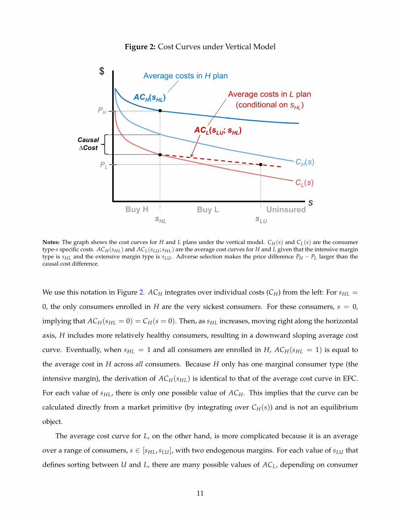
Figure 2: Cost Curves under Vertical Model
$
sBuy H Buy L Uninsured
ACL(sLU; sHL)
ACH(sHL)
Average costs in H plan
Average costs in L plan (conditional on sHL)PH
PL
sHL sLU
Causal ∆Cost
Notes: The graph shows the cost curves for H and L plans under the vertical model. CH(s) and CL(s) are the consumertype-s specific costs. ACH(sHL) and ACL(sLU ; sHL) are the average cost curves for H and L given that the intensive margintype is sHL and the extensive margin type is sLU . Adverse selection makes the price difference PH − PL larger than thecausal cost difference.
We use this notation in Figure 2. ACH integrates over individual costs (CH) from the left: For sHL =
0, the only consumers enrolled in H are the very sickest consumers. For these consumers, s = 0,
implying that ACH(sHL = 0) = CH(s = 0). Then, as sHL increases, moving right along the horizontal
axis, H includes more relatively healthy consumers, resulting in a downward sloping average cost
curve. Eventually, when sHL = 1 and all consumers are enrolled in H, ACH(sHL = 1) is equal to
the average cost in H across all consumers. Because H only has one marginal consumer type (the
intensive margin), the derivation of ACH(sHL) is identical to that of the average cost curve in EFC.
For each value of sHL, there is only one possible value of ACH. This implies that the curve can be
calculated directly from a market primitive (by integrating over CH(s)) and is not an equilibrium
object.
The average cost curve for L, on the other hand, is more complicated because it is an average
over a range of consumers, s ∈ [sHL, sLU ], with two endogenous margins. For each value of sLU that
defines sorting between U and L, there are many possible values of ACL, depending on consumer
11

sorting between H and L. This fact makes it impossible to plot a single fixed ACL curve as we did
with ACH. Nonetheless, it is possible to plot ACL(sLU) conditional on sHL(P). We denote this curve
ACL(sLU ; sHL) and illustrate it with a dashed line in Figure 2. There are many such iso-sHL plots of
ACL (not pictured) that hold PH fixed at various levels. The leftmost point of the ACL curve depends
on the sHL cutoff type determined by PH. Higher values of sHL imply that ACL(sLU ; sHL) starts from
a higher point. Just as ACH equals CH at s = 0, ACL equals CL at s = sHL. Moving rightward from
s = sHL, plan L adds more relatively healthy consumers, resulting in a downward sloping average
cost curve.
In summary, while ACH is fixed and does not depend on the price of L, ACL is an equilibrium
object in that it changes as PH, and therefore sHL, changes. This implies that the average cost of L
and thus the price of L in equilibrium depends on the price of H. Recognizing such dependencies is
critical for analyzing policy interventions. For example, a subsidy targeted to H that results in a lower
(net) PH and a larger H enrollment (a rightward-shifted sHL) would cause the leftmost point on ACL
to shift down and rightward and would cause the curve to have a less-steep slope. In a competitive
market, this would likely result in a lower PL, causing additional consumers to enter the market.
2.3 Competitive Equilibrium
We consider competitive equilibria where plan prices, Pe, exactly equal their average costs:10
PH = ACH (P) and PL = ACL (P) (6)
In some settings, there will be multiple price vectors that satisfy this definition of equilibrium, includ-
ing vectors that result in no enrollment in one of the plans or no enrollment in either plan. Because
of this, we follow Handel, Hendel and Whinston (2015) and limit attention to equilibria that meet the
requirements of the Riley Equilibrium (RE) notion. We discuss these requirements and provide an
algorithm for empirically identifying the RE in Appendix C.3.
With the outside option of uninsurance, the equilibration process for the prices of H and L dif-
fers somewhat from the more familiar settings explored by EFC and Handel, Hendel and Whinston
(2015). In those settings, it is assumed that all consumers choose either H or L. Assuming full in-
10This definition of equilibrium prices differs slightly from the definition of Einav, Finkelstein and Cullen (2010) whoconsider a "top-up" insurance policy where only the price of H is required to be equal to its average cost, while the price ofL is fixed. It is consistent, however, with the definition of Handel, Hendel and Whinston (2015)
12

surance conveniently simplifies the equilibrium condition from two expressions to one: Namely, that
the differential average cost must be set equal to the differential price.
Figure 3: Determination of Equilibrium with H, L, and Outside Option
(a) Determination of Extensive Margin (sLU)
$
s
WL
Buy H Uninsured
WH 1. Availability of L plan at PLimplies extensive margin (=sLU)
Buy L
PL
sLU
ACH(sHL)
(b) Determination of PH
$
s
WL
DH(PL0)
PL
Buy H Buy L Uninsured
WH
Buy L
2. Intersection of implied DHcurve and ACH determines PH
e
PHe(PL) ACH(sHL)
sLUsHL
(c) Determination of ACL
$
s
WL
ACH(sHL)PH
Buy H Buy L
3. Intensive margin (=sHL(PH)) implies ACL curve
ACL(sLU; sHL)
sHL
(d) Determination of PL
$
s
WL
PH
Buy H Buy L
4. Intersection of ACL and WLcurves determines PL
e
UninsuredBuy L
ACL(sLU; sHL)
PLe (PH)
ACH(sHL)
sLUsHL
Notes: Figures show how competitive equilibrium is determined in the vertical model with H and L plans and an outsideoption (uninsured). Panels (a) and (b) show the determination of PH(PL): a value of PL implies the extensive margin (sLU),which in turn implies the demand curve for H and the equilibrium PH . Panels (c) and (d) show the determination ofPL(PH): a value of PH implies the intensive margin (sHL), which implies ACL and the equilibrium value of PL.
To provide intuition for determining the equilibrium in our more complex setting, we build up
from the classic case considered by EFC, which includes only H and U as plan options.11 The EFC
11The correct analogy from EFC to our framework considers the choice between H and U rather than between H and Lbecause the distinguishing feature of U is that its price is exogenously determined, like the lower coverage option in the
13
equilibrium can be seen in Panel (a) of Figure 3, if one ignores the WL curve. It is defined by the
intersection of WH and ACH, which determines the competitive equilibrium price. Absent an L plan,
any s-type whose WTP for H exceeds the price of H will buy H and all other s-types will opt to
remain uninsured.
We next add L to the EFC choice set. To illustrate the equilibrium, we proceed in four steps,
corresponding to the four panels in Figure 3. Panels (a) and (b) show how PH is determined, given
a fixed price of L. Panel (a) shows that the fixed PL implies a given extensive margin cutoff, sLU .
Panel (b) shows that this in turn implies an H plan demand curve, DH(PL) (in dashed black). The
intersection of DH(PL) with H’s average cost curve determines PH and the intensive margin cutoff
sHL. This process determines the reaction function PeH(PL), which is the break-even price of H for a
given price of L.
Panels (c)-(d) of Figure 3 show how PL is determined, given a fixed PH. Panel (c) shows that the
fixed PH implies a given intensive margin cutoff (sHL), which in turn fixes the ACL curve. Panel (d)
shows how the intersection of ACL with WL determines PL and the extensive margin cutoff sLU . This
process determines the reaction function PeL(PH), which gives the break-even price of L for a given
fixed price of H.
In equilibrium, the reaction functions must equal each other: PH = PeH(PL) and PL = Pe
L(PH).
Figure 4 depicts the equilibrium, including the ACL and DH curves as dashed lines. These dashed
lines are themselves equilibrium outcomes, even holding fixed consumer preferences and costs. In
other words, there were many possible “iso-sHL” ACL curves and many possible “iso-PL” DH curves.
The equilibrium vector of prices are the prices at which demand for L generates the equilibrium
DH(PeL) and this demand for H simultaneously implies the equilibrium ACL(sHL) curve.
2.4 Social Welfare
We now show how our framework can be used to assess the welfare consequences of different poli-
cies. We define social welfare in the conventional way, as total social surplus. We provide a formal
definition below, but we start by showing what we mean graphically. In order to make the figures
simpler and more intuitive, we set CU , the social cost of uninsurance, equal to zero. We nonetheless
allow for a positive social cost of uninsurance in our empirical application below.
EFC setting.
14

Figure 4: Final Equilibrium
$
s
WL
Buy H Buy L
ACL(sLU; sHL)
UninsuredBuy L
WH
sLU
ACH(sHL)
sHL
DH(PLe)
PLe (PH)
PHe(PL)
Notes: The graph shows the final equilibrium under the vertical model with two plans (H and L) and an outside option(U). The black dots mark the key intersections defining equilibrium prices and sorting. The intersection of ACL and WLdetermines PL and the extensive margin type (sLU). The DH curve starts at this extensive margin (where it equals WH), andits intersection with ACH determines PH and the intensive margin type (sHL). This sHL type marks the start of the ACLcurve (where it equals CL).
To build intuition, we start in Panel (a) of Figure 5 by illustrating the case where L is a pure cream-
skimmer. That is, L has low average costs because it attracts low-cost individuals, but it has no causal
effect on costs, so CL = CH for any individual. For this case, given WH, WL, and CL = CH we can find
total social surplus for any allocation of consumers across plans described by the equilibrium cutoff
values seHL and se
LU .
Panel (a) of Figure 5 shows that social surplus consists of two pieces. The first piece (ABHG)
is the social surplus for consumers purchasing H, given by the area between WH and CL = CH for
consumers with s < sHL. The second piece (EFIH) is the social surplus for consumers purchasing L,
given by the area between WL and CL = CH for consumers with s ∈ [sHL, sLU ]. Panel (a) of Figure
5 also illustrates foregone surplus for the allocation of consumers across plans. Here, the foregone
surplus consists of three components. The first is the foregone surplus due to the fact that consumers
with s ∈ [sHL, sLU ] purchased L when they would have generated more surplus by purchasing H, and
it is described by the area between WH and WL for these consumers (BCFE). The second component
15

is the foregone surplus due to the fact that consumers with s > sLU did not purchase insurance
when they would have generated positive surplus by purchasing H, and it is described by the area
between WH and max{WL, CL} (CDJF). We refer to these two components as “intensive margin loss”.
The third component is the foregone surplus due to the fact that consumers with s ∈ [sLU , s∗LU ] did
not purchase insurance when they would have generated positive surplus by purchasing L, and it is
described by the area between WL and CL for those consumers.
The figure thus shows how our graphical framework can be used to estimate welfare for any
allocation of consumers across H, L, and U. Further, the framework makes it easy to determine
the optimal allocation of consumers between insurance and uninsurance and between H and L. In
the case of the particular demand and cost primitives drawn in Panel (a), the optimal allocation of
consumers across plans is for all consumers to be in H. If H were not available, however, the optimal
allocation of consumers across L and U would consist of all consumers with s < s∗LU purchasing L
and all other consumers remaining uninsured.
In Panel (b) of Figure 5, we show how our framework can also accommodate the case where it is
efficient for some consumers to be enrolled in L rather than in H and for others to remain uninsured
rather than be enrolled in L. To do this, we change the assumption that L is a pure cream-skimmer and
instead assume that costs in H are higher than in L for each consumer and that the cost gap is constant
across consumers: ∆CHL(s) ≡ CH(s)− CL(s) = δ > 0. Intuitively, in this scenario consumers prefer
H because it provides more or better services—at a higher cost to the insurer. It is convenient to
define a new curve WNetH (s) = WH(s)− ∆CHL(s), or WTP for H net of the incremental cost of H vs.
L. Under the assumption that δ is constant, WNetH (s) will be parallel to and below WH. This is shown
in Panel (b) of Figure 5: As L’s cost advantage over H increases, WNetH shifts further down.12
Given this new WNetH curve, social welfare is still fully characterized by the three curves, WNet
H ,
WL, and CL, and social surplus and foregone surplus are defined in a similar manner to Panel (a).
Social surplus still consists of two components. The first is the surplus generated by the consumers
enrolled in H, and it is characterized by ABHG, the area between WNetH and CL for consumers with
s < sHL.13 This component is smaller than it was in Panel (a) due to the fact that now H has higher
costs than L. In Panel (b) it is thus less socially advantageous for these consumers to be enrolled in
12Heterogeneity in L’s cost advantage across s types could also be accommodated and would result in WNetH not being
parallel to WH .13To see this, note that this gap is equal to WNet
H (s)− CL(s) = WH(s)− (CH(s)− CL(s))− CL(s) = WH(s)− CH(s).
16

Figure 5: Welfare
(a) Welfare when L Is a Pure Cream-Skimmer
$
sUninsuredBuy H
WL(s)
A
B
C
E
F
G Market Surplus
I
H
WH (s)
DJ
Intensive Margin Loss
Extensive Margin Loss
Buy L∗
(b) Welfare when L Has a Cost Advantage
$
sUninsuredBuy H
A
B
E
F
G
Buy L
I
H
WHNet(s) = WH(s) – ∆CHL(s)
DJ
Causal cost difference b/n H and L
K
Too many uninsured
WL(s)
Intensive Margin Loss
Extensive Margin Loss
WH (s)
Market Surplus
Too many in LBuy L
∗ ∗
Notes: The graphs show welfare given equilibrium prices Pe and implied consumer sorting between H, L, and uninsured.Panel (a) shows the case where the L plan is a pure cream-skimmer (∆CHL = CH(s)− CL(s) = 0), while panel (b) showsthe case where L has a causal cost advantage (∆CHL > 0). The market surplus is shaded in green; the loss due to intensivemargin misallocation (between H and L) is shaded in red; and the loss due to extensive margin misallocation (between Land U) is shaded in thatched red.
17
H vs. L. The second component is the surplus generated by the consumers enrolled in L, and it is
characterized exactly as before by EFIH, the area between WL and CL for consumers with seHL < s <
seLU . Foregone surplus is illustrated in the figure in Panel (b) similar to the illustration in Panel (a).14
In summary, Figure 5 shows how our model can accommodate settings in which it is not socially
efficient for all consumers to be enrolled in H or even in L, such as settings where there is moral
hazard, administrative costs, etc.
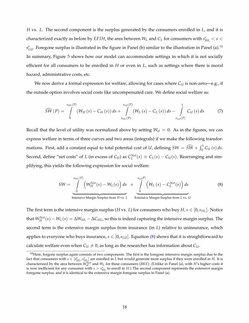
We now derive a formal expression for welfare, allowing for cases where CU is non-zero—e.g., if
the outside option involves social costs like uncompensated care. We define social welfare as:
SW (P) =
sHL(P)∫0
(WH (s)− CH (s)) ds +
sLU(P)∫sHL(P)
(WL (s)− CL (s)) ds−1∫
sLU(P)
CU (s) ds (7)
Recall that the level of utility was normalized above by setting WU = 0. As in the figures, we can
express welfare in terms of three curves and two areas (integrals) if we make the following transfor-
mations. First, add a constant equal to total potential cost of U, defining SW = SW +∫ 1
0 CU (s) ds.
Second, define “net costs” of L (in excess of CU) as CNetL (s) ≡ CL(s)− CU(s). Rearranging and sim-
plifying, this yields the following expression for social welfare:
SW =
sHL(P)∫0
(WNet
H (s)−WL(s))
ds
︸ ︷︷ ︸Intensive Margin Surplus from H vs. L
+
sLU P)∫0
(WL (s)− CNet
L (s))
ds
︸ ︷︷ ︸Extensive Margin Surplus from L vs. U
(8)
The first term is the intensive margin surplus (H vs. L) for consumers who buy H, s ∈ [0, sHL]. Notice
that WNetH (s)−WL(s) = ∆WHL−∆CHL, so this is indeed capturing the intensive margin surplus. The
second term is the extensive margin surplus from insurance (in L) relative to uninsurance, which
applies to everyone who buys insurance, s ∈ [0, sLU ]. Equation (8) shows that it is straightforward to
calculate welfare even when CU 6= 0, as long as the researcher has information about CU .
14Here, forgone surplus again consists of two components. The first is the foregone intensive margin surplus due to thefact that consumers with s ∈ [se
HL, s∗HL] are enrolled in L but would generate more surplus if they were enrolled in H. It ischaracterized by the area between WNet
H and WL for these consumers (BKE). (Unlike in Panel (a), with H’s higher costs itis now inefficient for any consumer with s > s∗HL to enroll in H.) The second component represents the extensive marginforegone surplus, and it is identical to the extensive margin foregone surplus in Panel (a).
18
3 Two-Margin Impacts of Risk Selection Policies
In this section, we use our model to assess the consequences of three policies commonly used to com-
bat adverse selection in insurance markets: benefit regulation, the mandate penalty on uninsurance,
and risk adjustment transfers. Each of these policies is targeted at one margin of adverse selection,
but our model shows how they affect the other. We discuss each policy in turn and provide graphical
illustrations for their consequences. We conclude with a discussion of other policies where cross-
margin impacts on selection may be relevant, including behavioral interventions targeting take-up.
3.1 Benefit Regulation
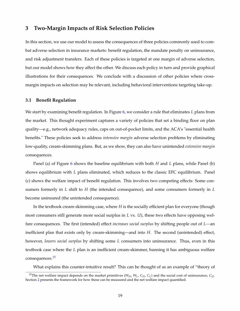
We start by examining benefit regulation. In Figure 6, we consider a rule that eliminates L plans from
the market. This thought experiment captures a variety of policies that set a binding floor on plan
quality—e.g., network adequacy rules, caps on out-of-pocket limits, and the ACA’s "essential health
benefits." These policies seek to address intensive margin adverse selection problems by eliminating
low-quality, cream-skimming plans. But, as we show, they can also have unintended extensive margin
consequences.
Panel (a) of Figure 6 shows the baseline equilibrium with both H and L plans, while Panel (b)
shows equilibrium with L plans eliminated, which reduces to the classic EFC equilibrium. Panel
(c) shows the welfare impact of benefit regulation. This involves two competing effects: Some con-
sumers formerly in L shift to H (the intended consequence), and some consumers formerly in L
become uninsured (the unintended consequence).
In the textbook cream-skimming case, where H is the socially efficient plan for everyone (though
most consumers still generate more social surplus in L vs. U), these two effects have opposing wel-
fare consequences. The first (intended) effect increases social surplus by shifting people out of L—an
inefficient plan that exists only by cream-skimming—and into H. The second (unintended) effect,
however, lowers social surplus by shifting some L consumers into uninsurance. Thus, even in this
textbook case where the L plan is an inefficient cream-skimmer, banning it has ambiguous welfare
consequences.15
What explains this counter-intuitive result? This can be thought of as an example of “theory of
15The net welfare impact depends on the market primitives (WH , WL, CH , CL) and the social cost of uninsurance, CU .Section 2 presents the framework for how these can be measured and the net welfare impact quantified.
19
Figure 6: Impact of Benefit Regulation
(a) No benefit regulation
$
s
WLACH(sHL)
UninsuredBuy L
DH( )
WH
Buy H
ACL(sLU;sHL)
(b) Plan L eliminated
$
s
ACH(sHL)
Uninsured
DH(PH) = WH
Buy H
Buy H instead of L
∗ ∗
Uninsured instead of L
(c) Welfare Impacts of Eliminating L Plan
H instead of L
$
sUninsuredBuy H
WL(s)
A
B
C
E
F
G
I
H
WHNet(s) = WH(s) – ∆CHL(s)
DJ
∗
U instead of L
K
L
(+)
Intensive Margin: Gain from shift L to H
(-)
Extensive Margin: Loss from newly uninsured
MN
Notes: The figure shows the impact on equilibrium (panels a and b) and welfare (panel c) of a benefit regulation thateliminates the L plan. This thought experiment captures a variety of policies that set a binding floor on plan quality,thus eliminating low-quality plans. For welfare impacts, we show the textbook case where H is the efficient plan for allconsumers and L is more efficient than U.
the second best”-style interactions that emerge with two margins of selection. Regulation that bans
a pure cream-skimming L plan addresses an intensive margin selection problem. But it has the unin-
tended side effect of worsening the extensive margin selection problem of too much uninsurance. Put
differently, a pure cream-skimming L plan adds no social value within the market, but by segmenting
the healthiest people into a low-price plan, it can improve welfare by bringing new consumers into
20

the market.16
3.2 Mandate Penalty on Uninsurance
Next we consider the consequences of a mandate penalty for remaining uninsured (choosing U).
The analysis is also applicable for analyzing the effect of providing larger insurance subsidies, which
likewise reduce consumers’ net price of buying insurance relative to remaining uninsured.
The mandate penalty has both a direct effect and an indirect effect through equilibrium price
adjustments. The direct effect of a mandate penalty is to increase the demand for insurance. Panel
(a) of Figure 7 shows this via an upward shift in WL and WH by $M, reflecting that both become
cheaper relative to U (whose utility and price are normalized to zero). As a result of this shift, some
people who were previously uninsured buy insurance in the L plan. This is the intended effect of the
penalty.
Panel (b) depicts the unintended, equilibrium effects of the penalty. By definition under extensive
margin adverse selection, the newly insured individuals are relatively healthy. Because they buy the
low-price L plan, they lower L’s average costs (i.e., a movement down the ACL curve, not a shift in
the ACL curve) and therefore its price. The lower PL leads some consumers to shift on the intensive
margin from H to L—as captured by the downward shift in H’s demand curve, DH(PL). This is the
main unintended effect of the penalty: although it is intended to reduce uninsurance, the penalty
also shifts people toward lower-quality plans on the intensive margin.17
There is a second equilibrium effect from this shift in consumers from H to L. The consumers
who shift are high-cost relative to L’s previous customers, pushing up L’s average costs. In panel (b),
this is depicted via an upward shift in the ACL(PH) curve, which has to occur because of the higher
PH and the leftward shift in the marginal sHL type. The higher average costs in L partly offset the
fall in PL due to the mandate and dampen the impact of the mandate on the price of L. Thus our
model shows how and why cross-margin effects may make a mandate less effective than one would
predict from its direct effects alone: The penalty induces healthy people to enter the market but also
16Of course, this reasoning depends on the market stabilizing to a separating equilibrium where both H and L survive.If the market unravels to the L plan, insurance coverage will typically not be higher: the price of L will not be low (sinceit attracts all consumers), and because the quality of L is lower, uninsurance will typically be higher than in an H-onlyequilibrium where L is banned. Whether the market stabilizes to a separating equilibrium or unravels to L/upravels to Hdepends on the market primitives.
17We show in our simulations and in Appendix A that this prediction is largely robust to relaxing the vertical model. Itis driven by two properties: (1) that the newly uninsured are relatively healthy (extensive margin adverse selection), and(2) that the newly insured mostly choose the low-priced L plan.
21

Figure 7: Impact of Mandate Penalty on Uninsurance
(a) Direct Effect
$
s
WL
ACH
Buy H Buy L
ACL(sLU;sHL)
DH(PL)WH
WL + M
Direct Effect (intended): Penalty increases demand for insurance
WH + M
P0H
s0HL s0
LU sMLU
P0L
L instead of U
(b) Equilibrium Effect
P0L
s0HLsM
HL
$
sBuy H Buy L
DH(PL)
WL + M
Equilibrium Effect (unintended): Lower PL decreases demand for HWH + M
ACH
L instead of H
P0H
s0LU sM
LU
PML
ACL(sLU;sHL)
L instead of U
(c) Welfare Effects
$
s
WL
WHNet(s) = WH(s) – ∆CHL(s)
Extensive Margin: Gain from newly insured
(-)
Intensive Margin: Loss from shift H to L
Buy L
(+)
Buy H Unins.L instead of H
L instead of U
Notes: The figure shows the impact of a mandate penalty in our framework. Panel (a) shows the direct effect: higherdemand for insurance. Panel (b) shows the unintended equilibrium effect: an intensive margin shift from H to L. Panel (c)shows the welfare effects in the textbook case where H is the efficient plan for all consumers and L is more efficient than U.
induces relatively sick people to move from H to L. Nonetheless, as long as the original equilibrium
is stable, one can show that on net, a larger penalty decreases PL and uninsurance (see Appendix A
for a formal derivation).
Panel (c) of Figure 7 shows the welfare effects in the textbook case where H is the efficient plan
for all consumers. There are again competing effects: (intended) welfare gains from newly insured
22

consumers and (unintended) welfare losses from consumers moving from H to the lower-quality L
plan. Thus, the interaction of the two margins of selection makes the welfare impact of a mandate
ambiguous even in this textbook case. In the extreme, a penalty could even lead to a market where
high-quality contracts are unavailable to consumers (i.e., market unraveling to L).
3.3 Risk Adjustment Transfers
Of the three policies we consider, risk adjustment is the most difficult to illustrate graphically because
the policy adds new risk-adjusted cost curves (for both L and H) that crowd the figure. Additionally,
risk adjustment transfers cause RACH (the risk-adjusted cost curve) to become an equilibrium object
rather than a stable market primitive (like ACH), as any effects of selection into the market are at least
partially shared between L and H due to the risk-based transfers. Despite this complexity, because
risk adjustment is an important policy lever used to combat intensive margin selection, we illustrate
in Appendix B how it works in our graphical model. Specifically, in Figure A2 we graph how perfect
risk adjustment, where transfers perfectly capture all variation in CL across consumer types, affects
equilibrium outcomes.
We show that perfect risk adjustment has two effects. First, it causes the average cost curve for H
to rotate downward until it is flat. This rotation of the cost curve causes sHL to shift right, indicating
a shift of consumers from L to H. This is the intended effect of risk adjustment, and it is caused by a
transfer from L to H to compensate H for the externality imposed on it by intensive margin selection
from L. Second, it causes the average cost curve for L to both rotate and shift up.18 This change in
ACL causes sLU to shift left, indicating a shift of consumers from L to U. This is the unintended effect
of risk adjustment. It occurs because the transfer to H comes from L, resulting in an increase in L’s
costs and price, forcing some consumers out of the market.
While perfect risk adjustment is a useful thought experiment, most markets include an imperfect
form of risk adjustment where transfers are based on individual risk scores computed from diagnoses
appearing in health insurance claims. (See Geruso and Layton (2015) for an overview.) For instance,
in the ACA Marketplaces, the per-enrollee transfer to plan j is determined by the following formula:19
18The curve remains downward-sloping because perfect risk adjustment only addresses intensive margin selection, leav-ing selection on the extensive margin in place.
19The actual formula used in the Marketplaces is a more complicated version of this formula that adjusts for geography,actuarial value, age, and other factors. Our insights hold with or without these adjustments, so we omit them for simplicity.
23
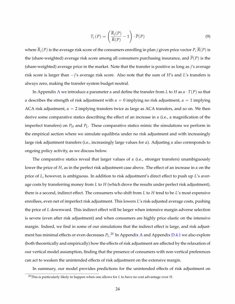
Tj (P) =
(Rj(P)R(P)
− 1
)· P(P) (9)
where Rj(P) is the average risk score of the consumers enrolling in plan j given price vector P, R(P) is
the (share-weighted) average risk score among all consumers purchasing insurance, and P(P) is the
(share-weighted) average price in the market. Note that the transfer is positive as long as j’s average
risk score is larger than −j’s average risk score. Also note that the sum of H’s and L’s transfers is
always zero, making the transfer system budget neutral.
In Appendix A we introduce a parameter α and define the transfer from L to H as α · T(P) so that
α describes the strength of risk adjustment with α = 0 implying no risk adjustment, α = 1 implying
ACA risk adjustment, α = 2 implying transfers twice as large as ACA transfers, and so on. We then
derive some comparative statics describing the effect of an increase in α (i.e., a magnification of the
imperfect transfers) on PH and PL. These comparative statics mimic the simulations we perform in
the empirical section where we simulate equilibria under no risk adjustment and with increasingly
large risk adjustment transfers (i.e., increasingly large values for α). Adjusting α also corresponds to
ongoing policy activity, as we discuss below.
The comparative statics reveal that larger values of α (i.e., stronger transfers) unambiguously
lower the price of H, as in the perfect risk adjustment case above. The effect of an increase in α on the
price of L, however, is ambiguous. In addition to risk adjustment’s direct effect to push up L’s aver-
age costs by transferring money from L to H (which drove the results under perfect risk adjustment),
there is a second, indirect effect. The consumers who shift from L to H tend to be L’s most expensive
enrollees, even net of imperfect risk adjustment. This lowers L’s risk-adjusted average costs, pushing
the price of L downward. This indirect effect will be larger when intensive margin adverse selection
is severe (even after risk adjustment) and when consumers are highly price elastic on the intensive
margin. Indeed, we find in some of our simulations that the indirect effect is large, and risk adjust-
ment has minimal effects or even decreases PL.20 In Appendix A and Appendix D.4.1 we also explore
(both theoretically and empirically) how the effects of risk adjustment are affected by the relaxation of
our vertical model assumption, finding that the presence of consumers with non-vertical preferences
can act to weaken the unintended effects of risk adjustment on the extensive margin.
In summary, our model provides predictions for the unintended effects of risk adjustment on
20This is particularly likely to happen when one allows for L to have no cost advantage over H.
24
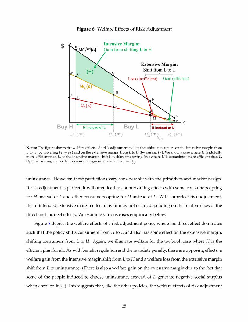
Figure 8: Welfare Effects of Risk Adjustment
$
s
WL(s)
A
F CG
H
KJ
WHNet(s)
EM
∗
L
N
(+)
Intensive Margin:Gain from shifting L to H
Loss (inefficient)
B
D
I
Buy LBuy H
Gain (efficient)
H instead of L U instead of L
Extensive Margin: Shift from L to U
Notes: The figure shows the welfare effects of a risk adjustment policy that shifts consumers on the intensive margin fromL to H (by lowering PH − PL) and on the extensive margin from L to U (by raising PL). We show a case where H is globallymore efficient than L, so the intensive margin shift is welfare improving, but where U is sometimes more efficient than L.Optimal sorting across the extensive margin occurs when sLU = s∗LU .
uninsurance. However, these predictions vary considerably with the primitives and market design.
If risk adjustment is perfect, it will often lead to countervailing effects with some consumers opting
for H instead of L and other consumers opting for U instead of L. With imperfect risk adjustment,
the unintended extensive margin effect may or may not occur, depending on the relative sizes of the
direct and indirect effects. We examine various cases empirically below.
Figure 8 depicts the welfare effects of a risk adjustment policy where the direct effect dominates
such that the policy shifts consumers from H to L and also has some effect on the extensive margin,
shifting consumers from L to U. Again, we illustrate welfare for the textbook case where H is the
efficient plan for all. As with benefit regulation and the mandate penalty, there are opposing effects: a
welfare gain from the intensive margin shift from L to H and a welfare loss from the extensive margin
shift from L to uninsurance. (There is also a welfare gain on the extensive margin due to the fact that
some of the people induced to choose uninsurance instead of L generate negative social surplus
when enrolled in L.) This suggests that, like the other policies, the welfare effects of risk adjustment
25

are theoretically ambiguous. Again, our model provides a simple framework for estimating the net
welfare effects given the relevant sufficient statistics (willingness-to-pay and cost curves).
3.4 Other Policies
The same price theory can be applied to other policies not explicitly discussed above. The key insight
is that anything that affects selection on one margin has the potential to affect selection on the other
margin, as firms adjust prices in equilibrium to compensate for the changing consumer risk pools.
For example, consider reinsurance, a federal policy in place from 2014 to 2016 in the ACA Mar-
ketplaces. Reinsurance has gained research attention for desirable market stabilization and incentive
properties (Geruso and McGuire, 2016; Layton, McGuire and Sinaiko, 2016) and has been adopted
in various forms by some states since the federal program expired.21 To the extent reinsurance is
implemented as a system of budget-neutral enforced transfers based on insurer losses for specific
conditions, it generates effects similar to those we document for risk adjustment. To the extent that
reinsurance is implemented as an external subsidy into the market by fees assessed on plans out-
side of the market (as in the ACA), it shares properties of both the mandate penalty (by providing
an overall insurance subsidy, making both H and L cheaper) and risk adjustment (by targeting the
subsidy to higher-cost enrollees more likely to be in H than in L), resulting in simultaneous extensive
and intensive margin effects that would be difficult to assess in models focusing only on one margin
or the other.22
It is important to understand that the cross margin effects are relevant not only for policies that
aim to address selection, but also for policies for which selection impacts are incidental or a nui-
sance. Handel (2013), for example, shows how addressing inertia through “nudging” can exacerbate
intensive margin selection in an employer-sponsored plan setting. Our model implies that in other
market settings, where uninsurance is a more empirically-relevant concern, there is a further effect of
nudging: Worsening risk selection on the intensive margin (i.e., increasing the market segmentation
of healthy enrollees into L and sick enrollees into H) through behavioral nudges may improve risk
selection on the extensive margin by pushing down the equilibrium price of L. This may counterbal-
21In policy practice, the term “reinsurance” is used to describe a wide gamut of regulatory interventions. see Harrington(2017) for a typology.
22In particular, like risk adjustment, reinsurance affects shifts the net average cost curves. Unlike risk adjustment, rein-surance will push both cost curves down, though typically having a larger effect on H’s cost curve due to H being morelikely to enroll the high-cost individuals who trigger reinsurance payments.
26

ance the welfare harm documented in Handel (2013). Similar insights apply to any behavioral inter-
vention that even incidentally affects the sorting of consumer risks (expected costs) across plans.23
Similarly, behavioral interventions intended to increase take-up of insurance, such as information in-
terventions or simplified enrollment pathways, may have important intensive margin consequences
similar to the effects of a mandate.
4 Simulations: Methods
Any set of reduced form estimates of willingness-to-pay and cost functions could be used to demon-
strate how our model can be applied empirically. Here, we draw on estimates of demand and costs
from the Massachusetts pre-ACA subsidized health insurance exchange, known as Commonwealth
Care or “CommCare,” from Finkelstein, Hendren and Shepard (2019), which we abbreviate as “FHS”.
We combine the FHS primitives, which describe lower-income consumers, with estimates for higher-
income Massachusetts households in the unsubsidized part of the individual market, known as
“CommChoice.” The latter estimates come from Hackmann, Kolstad and Kowalski (2015), which
we abbreviate as “HKK”. Both sets of demand and cost curves are well-identified using exogenous
variation in net consumer prices. FHS use a regression discontinuity design based on three house-
hold income cutoffs that generate discrete changes in consumer subsidies. HKK use a difference-in-
differences design leveraging the introduction of an uninsurance penalty in Massachusetts. Addi-
tional details about the estimation of the FHS and HKK curves can be found in Appendix C.1 as well
as in the respective papers.
We make two key modifications to the baseline FHS and HKK estimates. First, to allow for
broader policy counterfactuals, we extrapolate the curves over the full range of s-types. Second, we
combine the two sets of estimates to form one set of aggregated demand and cost curves, reflecting
ACA markets that include subsidized (low-income) and unsubsidized (high-income) enrollees. De-
tails on the construction of these demand and cost curves, as well as figures showing the final curves,
are in Appendix C.1.
23This is relevant not only as it relates to inertia (Polyakova, 2016), but also to misinformation (Kling et al., 2012; Handeland Kolstad, 2015; Bundorf, Polyakova and Tai-Seale, 2019), complexity (Ericson and Starc, 2016; Ketcham, Kuminoff andPowers, 2019), and other behavioral concerns. It is also relevant for non-behavioral policy changes in other markets, includ-ing Medicare. For example, Decarolis, Guglielmo and Luscombe (2017) document that intensive margin risk selection wasaffected by a Medicare policy change that allowed mid-year plan switching across Medicare Advantage plans. This couldhave—through an effect on costs and therefore prices—extensive margin impacts on who chooses Medicare Advantageversus Traditional Medicare.
27

Given these demand and cost curves, it is straightforward to estimate equilibrium prices and
allocations of consumers across H, L, and U under a given set of policies. Our method for finding
equilibrium is based on the approach described in Figure 3. We start by considering price vectors
resulting in positive enrollment in both H and L. For each potential PL we find the PH such that
PH = ACH and for each potential PH we find the PL such that PL = ACL. We then find where these
two “reaction functions” intersect. The intersection is the price vector at which both H and L break
even. We then also consider price vectors where there is zero enrollment in H, zero enrollment in
L, or zero enrollment in both H and L. We then use a Riley equilibrium concept to choose which
breakeven price vector is the equilibrium price vector.24 This method results in a unique equilibrium
for each policy environment we consider.
We then simulate market equilibrium under different specifications of two policies: a mandate
penalty (ranging from $0 to $60 per month) and risk adjustment transfers (ranging from zero to 3
times the size of ACA transfers). We study the effects of these policies in a 2×2 matrix of market
environments. The first dimension of the environment we vary is subsidy design, with two regimes:
(1) “ACA-like” subsidies that are linked to the price of the cheapest plan and (2) “fixed” subsidies set
at an exogenous dollar amount.25 In both subsidy cases, low-income consumers receive subsidies
only if they purchase H or L, and the subsidy is identical no matter which plan they choose. High-
income consumers do not receive subsidies.
The second dimension we vary is whether L is a pure cream-skimmer (i.e. CL(s) = CH(s) for
all s) or has a cost advantage (i.e. CL(s) < CH(s) for all s). FHS find no evidence that L has lower
costs than H in CommCare, motivating our cream-skimmer case. To illustrate another possibility, we
simulate the case where L has a 15% cost advantage (i.e. CL(s) = 0.85CH(s)). Of particular interest is
how the welfare consequences of risk adjustment and the uninsurance penalty vary across these two
cases. We explore these in Section 6.
24See Appendix C.4 for additional details. A breakeven price vector is a Riley equilibrium if there is no weakly profitabledeviation resulting in positive enrollment for the deviating plan that survives all possible weakly profitable responses tothat deviation. We describe how we empirically implement this equilibrium concept in the appendix.
25For (1) we follow the ACA rules by setting the subsidy such that the net-of-subsidy price of the index plan equals 4% ofincome for consumers at 150% of the federal poverty line (FPL) in 2011 (or $55 per month), the year on which our estimateddemand and cost curves are based. The ACA subsidy rules actually link the subsidy to the price of the second-lowest costsilver plan. Our subsidy rule mimics this rule in spirit (in a way that is compatible with our CommCare setting) by linkingthe subsidy to the price of L.
28

5 Simulation Results: Prices and Enrollment
In this section, we present results on how prices and market shares change under (1) stronger man-
date penalties and (2) stronger risk adjustment. In Appendix D.2 we also present results on how
prices and market shares change under benefit regulation, where we implement benefit regulation
by eliminating L from the consumers’ choice set. In Appendices D.4.1 and D.4.2 we explore the
sensitivity of our results to relaxing the vertical model and modifying the primitives (specifically,
consumers’ incremental WTP for H vs. L), finding that the key results are quite robust.
5.1 Mandate/Uninsurance Penalties
Figure 9 presents equilibrium market shares for each option, H, L, and U, under different levels of a
mandate penalty for remaining uninsured (PU ≡ M). We consider penalties in increments from $0
to $60.26 In all cases we include ACA-style risk adjustment (described in detail in Section 5.2 below).
The top two panels of Figure 9 contain the results for the case where L is a pure cream-skimmer. The
bottom two panels contain results for the case where L has a 15% cost advantage. The cases with
ACA-like price-linked subsidies are shown in the left panels and the cases with a fixed subsidy are
in the right panels.27 All results are also reported in Appendix Table A1.
For the two ACA-like subsidy cases (left), the patterns are qualitatively similar regardless of
modeling L as a cream skimmer (top) or as having a cost advantage (bottom). When there is no
mandate penalty, some consumers choose each of the three options, H, L, and U, though the share
in H is extremely low in the cost advantage case. As the penalty increases, the uninsurance rate
decreases, with no consumers remaining uninsured at a penalty of $60/month. However, there are
also intensive margin consequences: As the penalty increases, there is a shift of consumers from H
to L. In the case where L is a pure cream-skimmer, H’s market share decreases from 42% with no
penalty to 23% with a penalty of $60/month. This represents a significant decline in H’s market
share and a significant deterioration of the average generosity of coverage among the insured. In the
case where L has a 15% cost advantage (bottom), the patterns are similar, though H’s initial market
26We find that in all cases studied here, PU = 60 is sufficient to drive the uninsurance rate to 0 in the presence of ACArisk adjustment transfers.
27Fixed subsidies are equal to $275 in the case where L is a pure cream-skimmer and $250 in the case where L has a 15%cost advantage. These values were chosen in order to ensure that risk adjustment and the uninsurance penalty have someeffect on market shares. With subsidies that are “too large” no consumers opt to be uninsured and with subsidies that are“too small” no consumers opt to purchase insurance, making the simulated policy modifications uninformative.
29
Figure 9: Market Shares with Varying Mandate Penalty (M)
(a) ACA-like subsidy, L cream-skimmer (b) Fixed $275 subsidy, L cream-skimmer
(c) ACA-like subsidy, 15% L cost advantage (d) Fixed $250 subsidy, 15% L cost advantage
Notes: The figures show market shares for H, L, and uninsurance (U) from our simulations with varying sizes of themandate penalty (x-axis, in $ per month). The panels represent different subsidy designs and specifications for the L plan’scausal cost advantage vs. H (i.e., ∆CHL). In panels (a) and (b), L is a pure cream-skimmer (∆CHL = 0), while in panels (c)and (d) L has a 15% cost advantage. Panels (a) and (c) have “ACA-like subsidies” linked to the price of L, while panels (b)and (d) have fixed subsidies of the indicated dollar amounts.
share with no penalty is much lower (≈ 2%), so the intensive margin consequences are less stark.
The two fixed subsidy cases are presented in the right panels of Figure 9. When L is a pure
cream-skimmer (top), in the absence of a penalty consumers are split across H, L, and U. As the
penalty increases from zero, consumers move from U to L, the intended effect of the policy. At a
penalty of just under $30/month the influx of relatively inexpensive consumers into L causes PL to
get low enough relative to PH that some consumers previously in H begin to opt for L. As the penalty
continues to increase, consumers move into L from both U and H until the mandate reaches just over
$40/month and all consumers are enrolled in insurance. At this point 23% of the market is enrolled
in H and 77% of the market is enrolled in L. This represents an intended decline in the uninsurance
rate from 35% to 0% but also an unintended decline in H’s market share from 42% to 23%.28
28In the case where L has a 15% cost advantage, the penalty again decreases both the uninsurance rate (intended) andH’s market share (unintended), but H’s market share with a $0 penalty is so low (around 3.5%) that the decline in H’s
30

In each of the empirical cases we consider in Figure 9, a larger insurance mandate penalty has
the intended consequence of decreasing the portion of consumers opting to remain uninsured and the
unintended consequence of shifting consumers from H to L. This finding holds when we relax the
vertical assumptions of the model in Appendix Figure A9. 29 This is consistent with implications of
our graphical model as well as the comparative statics we outline in Sections 2 and 3. The unintended
intensive margin effect is most stark in the case where L is a perfect cream-skimmer, highlighting how
the market primitives can amplify the cross-margin impacts of policy changes.30
5.2 Risk Adjustment
We now consider the effects of risk adjustment. We start with risk adjustment transfers implied by
the ACA risk adjustment transfer formula (see Eq. 9). We first calculate risk scores for each individual
using the HHS-HCC risk adjustment model used in the ACA Marketplaces. (This is a straightforward
mechanical application of the regulator’s algorithm to our individual-level claims data.) We then use
those scores plus the FHS regression discontinuity design to estimate a “risk score curve” RA(s)
describing the average risk score across consumers of a given s-type. Because this curve is novel to
this paper and not estimated by FHS, we describe the estimation of it in Appendix C.2. We plot this
curve alongside the cost curve in Appendix Figure A4. It is apparent that while risk scores explain
part of the correlation between willingness-to-pay and costs, they do so only imperfectly. Specifically,
we find that risk scores account for about one-third of the correlation between willingness-to-pay
and costs, implying substantial selection on costs net of the ACA’s imperfect risk adjustment policy.
(Although incidental to our aims here, this is a novel finding.)
We use the risk score curve to determine the average risk scores for H and L for any given al-
location of consumers across H, L, and U. This is similar to constructing average cost curves from
marginal costs. We then enter these average risk scores into the risk adjustment transfer formula (Eq.
9) to determine the transfer from L to H for a given price vector T (P). Finally, we find the equilib-
rium prices. These satisfy PH = ACH(P) − T (P) and PL = ACL(P) + T (P) when L and H have
market share (to zero) is relatively insignificant.29In Appendix D.4.1 we explore the sensitivity of these results to the vertical model assumption, finding that the results
are largely robust to modest relaxation of the assumption. See Figure A9. In addition, in Appendix D.4.2 we show thatthese results are also robust to varying the incremental WTP for H vs. L.
30To see why the effect would be larger for the cream-skimmer case, note that for fixed consumer preferences, it isrelatively more difficult to achieve high levels of enrollment in H when L has an actual cost advantage versus when L hassimilar costs to H. This leads to lower enrollment in H even at low levels of the mandate penalty, and less opportunity fora reduction in H’s market share.
31
Figure 10: Market Shares with Varying Strength of Risk Adjustment (α)
(a) ACA-like subsidy, L cream-skimmer (b) Fixed $ 275 subsidy, L cream-skimmer
(c) ACA-like subsidy, 15% L cost advantage (d) Fixed $ 250 subsidy, 15% L cost advantage
Notes: The figures show market shares for H, L, and uninsurance (U) from our simulations with varying strength of riskadjustment α (on the x-axis). As described in text, α is a multiplier on the risk adjustment transfer: α = 0 implies no riskadjustment; α = 1 is baseline risk adjustment using the ACA formula; and α > 1 is over-adjustment. The panels representdifferent subsidy designs and specifications for the L plan’s causal cost advantage vs. H (i.e., ∆CHL). In panels (a) and (b),L is a pure cream-skimmer (∆CHL = 0), while in panels (c) and (d) L has a 15% cost advantage. Panels (a) and (c) have“ACA-like subsidies” linked to the price of L, while panels (b) and (d) have fixed subsidies of the indicated dollar amounts.
non-zero enrollment.
To vary the strength of risk adjustment transfers we maintain the original risk scores and struc-
ture of the transfer formula, but we multiply transfers by a scalar α (as in the comparative statics in
Appendix A) so that transfers from L to H are some multiple of the transfers implied by the ACA
formula. We allow α to vary from 0 (no risk adjustment) to 3 (risk adjustment transfers 3 times the
size of ACA transfers). The case of ACA transfers occurs where α = 1. This approach to evaluating
strengthening or weakening risk adjustment reflects real-world policy experimentation: The federal
government recently reduced α from 1 to 0.85 in the ACA Marketplaces and gave states the ability
to further reduce α.31 Our approach thus maps to feasible policy interventions, rather than assuming
31The reduction of α from 1 to 0.85 occurred when the federal government decided to “remove administrative costs”from the benchmark premium that multiplies insurer risk scores to determine transfers in the transfer formula describedby Eq. 9.
32

that the regulator can increase the predictive power of risk scores.
Equilibrium market shares for different levels of α in the cases without and with a cost advantage
for L are found in the top and bottom panels of Figure 10, respectively. Market shares under ACA-
like subsidies are presented in the left panels and market shares under fixed subsidies are found in
the right panels. Results are also found in Appendix Table A2. With ACA-like subsidies, patterns
are qualitatively similar when L is a pure cream-skimmer and when L has a 15% cost advantage. In
both cases, when there is no risk adjustment (α = 0), the market unravels to L: No consumers choose
H, and the market is split between L and uninsurance. As the strength of risk adjustment transfers
increases, consumers shift from L to H. This is the intended consequence of risk adjustment. When L
is a pure cream-skimmer, transfers about 1.25 times the size of ACA transfers are sufficient to cause
the market to “upravel” to H. When L has a 15% cost advantage transfers need to be 1.6 times the
size of ACA transfers to generate the same outcome. In both cases, there is no extensive margin
effect except at the level of α where the market initially upravels to H. At that point, there is a small
reduction in the uninsurance rate. This reduction is due to the fact that there the subsidy becomes
linked to the (higher) price of H instead of the (lower) price of L due to the exit of L from the market.
With the larger subsidy, more consumers purchase insurance.32
The right column of Figure 10 presents market shares under fixed subsidies with different levels
of α. Here, we again see that stronger risk adjustment transfers have the intended effect: Higher
levels of α result in more consumers choosing H instead of L. In the case where L is a pure cream-
skimmer, we see only a small extensive margin effect, with a small decrease in the uninsurance rate
as α increases. This is consistent with our comparative statics from Section 3: The direct effect of
increasing the transfer from L to H is more than fully offset by the indirect effect of the costliest
(net of imperfect risk adjustment) L enrollees leaving L and joining H, resulting in a decrease in PL
and a corresponding decrease in the uninsurance rate. (See Section 3 and Appendix A for a fuller
discussion of this result.)
On the other hand, in the case where L has a 15% cost advantage we see a different unintended
extensive margin consequence of stronger risk adjustment transfers: More consumers opt to remain
32This reduction seemingly goes against the intuition we present in Section 3 where we showed that in many cases riskadjustment may increase the uninsurance rate rather than decrease it as we see here. Note, however, that in the cases herethe subsidy is linked to the extensive margin price. This results in risk adjustment having no effect on the net-of-subsidyextensive margin price faced by the low-income consumers (except where L exits the market), limiting (and in this caseeliminating) any unintended extensive margin consequence.
33

uninsured. In this case, with no risk adjustment (α = 0) all insured consumers opt for L, with no
consumers choosing H and the market split between L and U. ACA risk adjustment transfers (α =
1) barely alter these market shares. As transfers are strengthened above ACA levels, consumers
begin to opt for H instead of L. At the higher levels of α, extensive margin consequences also start
to appear with some consumers exiting the market and opting for uninsurance. When transfers
are strengthened to two times the size of ACA transfers, the market upravels to H with all insured
consumers opting for H instead of L. At α = 2 the uninsurance rate reaches almost 50%, an increase
of 15 percentage points (60%) compared to the case with no risk adjustment. This indicates that this
shift of consumers to more generous coverage on the intensive margin had a substantial extensive
margin impact. We show that the same result holds when we relax the vertical model assumptions
in Appendix Figure A9.33
These results provide important lessons for where the unintended extensive margin effects of risk
adjustment will matter most. First, ACA-like price-linked subsidies protect against the unintended
extensive margin effects of risk adjustment, even when those subsidies are only targeted to the low-
income consumers making up 60% of the market (though there may be important effects on the size
of the subsidies themselves, and thus the cost to the government). Second, the unintended extensive
margin effects are more likely to occur when L has a larger cost advantage over H. In cases where L
and H have similar costs, extensive margin effects are likely to be small. But when L has a large cost
advantage, stronger risk adjustment can have significant effects on the portion of consumers in the
market who opt to be uninsured.
6 Simulation Results: Welfare
We next analyze the changes in social surplus associated with the policy simulations of Section 5. We
characterize welfare at a baseline equilibrium, then trace the gains and losses associated with illus-
trative policy changes, and finally determine optimal policy. Importantly, we show that the optimal
size of the mandate is dependent on the parameter determining the strength of risk adjustment and
vice versa. One straightforward implication is that if mandate penalties were altered by legislative
action or court outcomes, a constrained optimal response from a regulator would likely be to adjust
33In Appendix D.4.1 we explore the sensitivity of these results to the vertical model assumption, finding that the resultsare robust to modest relaxation of the assumption. See Figure A9. Also, in Appendix D.4.2 we show that these results arelargely robust to varying the incremental WTP for H vs. L.
34
risk adjustment strength in concert. (Unlike altering a mandate penalty, a regulator would typically
have authority to tune risk adjustment without further changes to law.)
We begin by noting the possibility that in many settings, social surplus may not be increased
by policies that increase insurance take-up or that move consumers from less generous coverage to
more generous coverage. This is because some consumers may not value insurance more than the
cost of providing it to them and may not value the incremental coverage provided by more generous
plans more than the incremental cost of providing that coverage. Further, we have shown above that
policies may have opposing effects on the intensive and extensive margins, increasing enrollment in
more generous coverage while simultaneously decreasing overall insurance take-up, or vice versa.
For these reasons, it is important to understand the effects of policies not just on market allocations
(which Section 5 presents), but also on welfare.
As discussed in Section 2, it is straightforward to estimate overall social surplus associated with
some equilibrium market outcome (enrollment shares), given the WNetH = WH − (CH − CL); WL;
and CNetL = CL − CU curves. From Section 4, we have all necessary primitives except CU . From
Section 5, we have equilibrium market shares under a variety of policy environments, which we
can contrast to the social optimum defined by the primitives. Therefore, the only missing piece for
estimating welfare is the social cost of uninsurance. In Section 2 we assumed CU = 0 for simplicity.
However, this assumption ignores uncompensated care, care paid for by other state programs, or
more difficult-to-measure parameters like a social preference against others being uninsured. Because
we do not have any way to directly measure the social cost of uninsurance, we specify it as linked to
the observed type-specific cost of enrolling in H. We write the social cost of uninsurance for type s
as:
CU(s) =(1− d)CH(s)
1 + φ+ ω (10)
where d is the share of total uninsured healthcare costs that the uninsured pay out of pocket, φ is the
assumed moral hazard from insurance, and ω is some fixed cost of uninsurance. For d and φ, we use
the values as derived from Finkelstein, Hendren and Shepard (2019) and assume that d = 0.2 and
φ = 0.25.34 We set the fixed cost ω = −$97 per month, which is the ω value consistent with 95% of
the population being optimally insured when L has a 15% cost advantage.
34We note that without this assumption (i.e. if we assume CU = 0), it is inefficient for any consumer to purchaseinsurance, as no consumer values either H or L more than the cost of enrolling them in H or L. This fact plus a fulldiscussion of the derivation of the assumed values of d and φ can be found in Finkelstein, Hendren and Shepard (2019).
35

Before showing how to use our graphical model to estimate welfare, we provide an important
caution: As is standard in the literature, our welfare estimation depends critically on inferring con-
sumer valuation of H and L from estimates of the demand-response to exogenous variation in the
prices of these products. Our welfare estimates are accurate only to the extent that demand curves
accurately reflect true valuations. Behavioral frictions might cause consumer demand to deviate from
valuations (Handel, Kolstad and Spinnewijn, 2019). Liquidity constraints could also cause valuation
and demand to diverge (Casaburi and Willis, 2018). A separate issue is that our specification of CU
is ad hoc and may not reflect the actual social costs of uninsurance. Indeed, many of our welfare con-
clusions will necessarily be sensitive to our assumptions about CU . (We present welfare results for
alternative assumptions about CU in Appendix D.3.2.) We thus present these welfare results to (1)
show how our framework can be used to analyze welfare and (2) to build intuition for the welfare
trade-offs involved with various policies. But we do not make any normative conclusions about the
specific market we study.
Importantly, considerations about choice frictions or about the difficulty of measuring CU do not
threaten the use of our model for the positive analysis of Section 5, which consists of predictions of
prices and market shares under different counterfactual mandate penalties and risk adjustment. Such
predictions do not rely on assumptions about CU or about demand reflecting underlying consumer
valuation.
6.1 Welfare and Changes to Risk Adjustment
We now show how to estimate welfare with our graphical model. For parsimony, we focus in the
main text on the case of strengthening risk adjustment transfers. In Appendix D.3 we show the case
of an uninsurance penalty. Figure 11 plots the empirical analogs to our welfare figures from Section
2. Panel (a) depicts foregone surplus relative to the social optimum under a baseline case with ACA
risk adjustment (α = 1), no mandate penalty, and a fixed subsidy equal to $250. Panel (b) depicts
the difference in social surplus between the baseline case and a similar case where risk adjustment
is strengthened (α = 2), reflecting the simulation reported in the bottom-right panel of Figure 10.
Instead of plotting CL, we plot CNetL = CL − CU , as in Eq. (8) to account for the fact that CU 6= 0. We
also plot WNetH = WH − (CH − CL) as in Section 2.
In Panel (a), we indicate the equilibrium s cutoffs for α = 1. The intensive margin equilibrium
36

Figure 11: Empirical Welfare Effects from Simulations
(a) Baseline Sorting and Welfare Loss (b) Welfare Effects of Stronger Risk Adjustment
Notes: In both panels (a) and (b), we assume that there is a fixed subsidy equal to $250 and L has a 15% cost advantage overH. Further, 60% of the population is low-income and 40% of the population is high-income, so WTP curves are weightedsums of both types. Panel (a) shows welfare losses in this setting under no mandate and α = 1, relative to efficient sorting.Efficient cutoffs are indicated with a * while equilibrium outcomes are denoted with an e superscript. Panel (b) showswelfare changes under a risk adjustment policy where α = 2, relative to the baseline risk adjustment policy where α = 1.
cutoff is seHL and the extensive margin cutoff is se
LU . Thus, consumers with s < seHL enroll in H,
consumers with seHL < s < se
LU enroll in L, and consumers with s > seLU remain uninsured.
Efficient sorting of consumers across options is indicated by s∗ cutoff types. Consumers with
s < s∗HL should be in H, consumers with s∗HL < s < s∗LU should be in L, and the few consumers with
s > s∗LU should be uninsured to maximize social surplus. In panel (a) of Figure 11, we depict the
foregone surplus in the baseline ACA setting with shaded areas. Intensive margin foregone surplus
(lost surplus due to consumers choosing L instead of H) is indicated by the welfare triangle ABC,
representing a welfare loss of $19.71.35 Extensive margin foregone surplus is represented by the
welfare triangle DEF. Welfare loss on this margin amounts to $33.47. Combining these, the (average
per consumer) foregone surplus in the baseline setting in panel (a) of Figure 11 is thus $53.18.
Panel (b) of Figure 11 shows the welfare consequences of strengthening risk adjustment. To
show the effects of strengthening risk adjustment, we increase α from 1 to 2, so that risk adjustment
transfers are increased to two-times the ACA transfers. We hold all other policy parameters fixed.
Recall from the bottom-right panel of Figure 10 that moving from α = 1 to α = 2 in this setting shifts
35These shapes are more triangle-ish than triangular.
37

nearly 60% of consumers in the market from L to H but also shifts 13% of consumers in the market
from L to U. Overall, no consumers remain in L when α = 2.
The first effect of increasing α is the intended consequence of risk adjustment, and here it implies
both welfare gains and losses. Welfare gains occur when consumers whose incremental valuation
for H vs. L exceeds the incremental cost of H vs. L (i.e. those with WNetH (s) > WL(s)) enroll in H
instead of L. These gains are represented by the green welfare triangle ABC, and they amount to
$19.71. Welfare losses occur when consumers whose incremental valuation for H vs. L is less than
the incremental cost of H vs. L (i.e. those with WNetH (s) < WL(s)) enroll in H instead of L as L
unravels. These offsetting welfare losses occur when “too many” consumers enroll in H, and they
are represented by the red welfare triangle CDE and amount to $19.24. In other settings, where it
is always more efficient for consumers to be enrolled in H instead of L (such as the pure cream-
skimming case), there will only be welfare gains on this margin. In the case of panel (b) of Figure
11, the two effects nearly cancel each other out so that the net welfare gain due to the intended
consequence of shifting consumers from L to H amounts to just $0.47.
The second effect of increasing α is the unintended consequence of risk adjustment, and here it
implies welfare losses. Because risk adjustment leads to a higher price of L, some consumers exit the
market, increasing the uninsurance rate. In this case, all consumers who exit the market value insur-
ance more than the (net) cost of insuring them, CNetL = CL − CU , causing the welfare consequences
of this shift of consumers out of the market to be unambiguously negative. The size of the welfare
loss is represented by the area of EFGH, which we estimate to be $68.30. Combining the intended
and unintended consequences of risk adjustment, we estimate that in this setting doubling risk ad-
justment transfers by shifting from α = 1 to α = 2 would decrease welfare by $67.83, on average per
consumer.
Welfare results for all settings studied in Figures 9 and 10, for the full range of levels of α, and
under different assumptions about CU are found in Appendix D.3.2. These results indicate that under
our baseline assumption of CU (Equation 10), with ACA-like subsidies, increasing the strength of risk
adjustment transfers always improves welfare when L is a pure cream-skimmer. In this case, there
is no effect of risk adjustment on the extensive margin due to the linkage of the subsidy to the price,
leaving only intensive margin consequences. The intensive margin effects of moving consumers
from L to H are also unambiguously positive, as it is inefficient for any consumer to be enrolled in L
38

vs. H. When L has a cost advantage, increasing the strength of risk adjustment transfers improves
welfare given low initial levels of α but decreases welfare given higher initial levels of α, with the
welfare-maximizing risk adjustment policy having an α around 1.25, or 1.25 times the strength of
ACA risk adjustment transfers. This non-monotonic result is due to the fact that increases in α from
low initial levels of α induce only those consumers who value H highest relative to L to enroll in H,
with consumers whose incremental WTP does not exceed their incremental cost remaining enrolled
in L.
With fixed subsidies, the welfare consequences again depend on whether L has a cost advantage.
Recall that when L is a pure cream-skimmer, extensive margin consequences of risk adjustment are
limited. It is inefficient for any consumers to be enrolled in L vs. H in the cream-skimmer case,
implying that the intensive margin effects of moving consumers from L to H are unambiguously
positive. When L has a cost advantage, patterns in the fixed subsidy case are similar to the ACA-like
subsidy case, with welfare increasing with the strength of risk adjustment at low initial levels of α
and decreasing at higher levels. Here, in addition to moving some consumers who should not be
in H into H, stronger risk adjustment also pushes consumers out of the market, further worsening
the negative effects of risk adjustment. Overall, risk adjustment is most likely to improve welfare
in a setting with ACA-like subsidies and when L plans do not have a cost advantage. However,
policymakers should be cautious when strengthening risk adjustment in settings where subsidies are
fixed and/or plans are heterogeneous in their cost structures.
6.2 Optimality under Interacting Policies
The findings above suggest the necessity of a second-best approach to policy: optimal extensive
margin policy (penalties and subsidies) will often depend on the intensive margin policies (risk ad-
justment and benefit regulation) currently in use in a market. Here we show how our model can be
used to assess optimal policy, allowing for these interactions.
We again consider uninsurance penalties and risk adjustment. We compute social welfare over
a grid of uninsurance penalties and levels of α. We do this for the case in which L has a 10% cost
advantage and low-income consumers (who comprise 60% of the market) receive a fixed subsidy
equal to $250 when purchasing insurance. The social cost of uninsurance is once again set to CU(s) =
0.25CH(s)− 97 as in the previous section. We “cherry-pick” this case because the two policies interact
39

Figure 12: Welfare under Interacting Extensive and Intensive Margin Policies
Notes: The figure shows social welfare outcomes (darker = higher welfare) from the model simulations under differentparameters for the strength of risk adjustment (α, x-axis) and for the size of the uninsurance mandate penalty ($ per month,y-axis). The key point is that the optimum for one policy depends on the other: with weak risk adjustment a weakermandate is optimal, while with strong risk adjustment a strong mandate is optimal.
in interesting ways. For completeness, we perform similar analyses for all other settings studied in
Figures 9 and 10. Results are reported in Appendix D.3.
Figure 12 presents the welfare estimates graphically as a heat map, where darker areas represent
higher values of social surplus.36 Under a 10% cost advantage, the socially efficient allocation is
for 33% of the population to be in H, 60% of the population to be in L, and the remainder to be
uninsured. We can examine how the optimal level of risk adjustment changes with different values
of the mandate penalty. The figure shows that in this setting, when the mandate penalty is high,
welfare is increasing in the strength of risk adjustment (i.e. higher α). At these high values of the
mandate penalty, all consumers purchase insurance, eliminating any potential unintended extensive
margin consequences. Under such high market enrollment, it is optimal to use strong risk adjustment
36Consider a given α, mandate combination that generates a level of welfare W(α, mandate). We scale/normalize theheat map shading as follows: Wnorm(α, mandate) = W(α,mandate)−min(W)
max(W)−min(W), where the maximum and minimum are taken
over all possible α, mandate combinations for the setting.
40
to sort more people into H instead of L. With low levels of the mandate penalty, however, risk
adjustment has important unintended extensive margin consequences. Thus, the benefits of shifting
consumers from L to H must be traded off against the costs of shifting consumers out of the market
and into U. The results in Figure 12 indicate that with a small penalty, social surplus is maximized at
1.25 < α < 1.5, somewhat stronger than ACA risk adjustment but weaker than the optimal level of α
under a strong penalty, which is > 1.5.
We can also use Figure 12 to consider the optimal mandate penalty for each level of α. With weak
risk adjustment, starting from low levels of the mandate penalty, social surplus is increasing in the
size of the penalty. However, starting from high levels of the penalty, the sign is opposite, with so-
cial surplus increasing rapidly as the penalty is reduced. This occurs because while a strong mandate
penalty increases social surplus by inducing consumers to enroll in insurance, it also has the first-
order offsetting effect of shifting consumers from H to L. Ultimately, an intermediate penalty level
(around $30) maximizes social surplus, though any level of the penalty below $40 achieves much
higher levels of social surplus than the level achieved by a penalty exceeding $40. When risk ad-
justment is strong, social surplus is increasing in the mandate penalty. Here, strong risk adjustment
causes the market to “upravel” to H, eliminating any potential unintended intensive margin conse-
quences of increasing the level of the penalty. With strong risk adjustment, a stronger mandate thus
only induces consumers to move from U to H, generating higher levels of social surplus.
In terms of optimal policy, Figure 12 reveals that social surplus is highest for an intermediate
level of both the uninsurance penalty and risk adjustment. Given such a combination of policies,
consumers sort themselves to each of H, L, and U, which is the socially efficient outcome in this
particular setting. Note that the lowest-surplus combinations are a strong mandate with weak risk
adjustment or a weak mandate with strong risk adjustment.
In Appendix D.3 we show that other settings have different optimal policies. In the case where
L is a pure cream-skimmer and subsidies are linked to prices (ACA-like subsidies), optimal policy
is to have strong risk adjustment (high α) and a weak mandate. In the case where L has a cost
advantage, a weak mandate with weak to moderate risk adjustment is the optimal policy. In all
cases, it is clear that these two policies interact with each other, implying that evaluating one policy
in isolation from the other can be misleading. Specifically, market designers should not only consider
consumer preferences for high- vs. low-quality coverage and consumer valuation of insurance but
41
also the interaction between intensive and extensive margin selection when determining the optimal
combination of policies.
7 Conclusion
Adverse selection in insurance markets can occur on either the extensive (insurance vs. uninsurance)
or intensive (more vs. less generous coverage) margin. While this possibility has been recognized for
a long time, most prior treatments of adverse selection focus on only one margin or the other. This
focus misses important cross-margin trade-offs inherent to many selection policies.
In this paper, we develop a simple graphical framework that generalizes the framework of Einav,
Finkelstein and Cullen (2010) by adding the option to remain uninsured. Our setup allows for and
highlights simultaneous selection on both margins. We use this framework to build intuition for the
unintended intensive margin consequences of extensive margin policies and vice versa. We show
that the extent to which these cross margin effects occur depends on the primitives of the market.
We also show that it is straightforward to take the graphical framework directly to the data with
variation that identifies two sets of demand and cost curves. We do this with estimates from Mas-
sachusetts and find that the extensive/intensive margin trade-off is empirically relevant for evalu-
ating the consequences of various policies. Specifically, (1) strengthening uninsurance penalties can
help some consumers by getting them into the market while hurting other consumers by inducing
them to enroll in lower-quality coverage, and (2) strengthening risk adjustment transfers can help
some consumers by inducing them to enroll in higher-quality coverage while hurting other con-
sumers by forcing them out of the market. Additionally, we find that price-linked subsidies for low-
income consumers can weaken some of these trade-offs (i.e. effects of risk adjustment and benefit
regulation) but not others (i.e. mandates/uninsurance penalties). Finally, we show that trade-offs
related to risk adjustment are often more pronounced when the advantageously selected plan has a
cost advantage.
Because many policies lead to coverage gains on one margin and coverage losses on the other, in
some cases the unintended effects of policies are first-order with respect to welfare. We show cases in
which the welfare losses from coverage losses on the unintended margin exceed welfare gains from
coverage gains on the intended margin. This happens most often with a penalty for choosing to be
uninsured.
42

The simplicity of our approach is not without some costs. The assumption of perfect vertical
ordering of demand, in particular, is required to maintain simplicity in the figures, though we show
in both theory and empirics that our results are largely robust to the relaxation of this assumption.
What matters is that the primary way in which plans are differentiated is vertically. Some of our
insights may differ in more complex markets, and these complexities are an important area for future
research.
The issues we highlight here are relevant for future reform of the individual health insurance
markets in the U.S. Many have observed that the overall quality of coverage available to consumers
is low in these settings, with most plans characterized by tight provider networks, high deductibles,
and strict controls on utilization. Additionally, others have observed that take-up is far from com-
plete, with many young, healthy consumers opting out of the market altogether and choosing to
remain uninsured (Domurat, Menashe and Yin, 2018). These two observations are consistent with
adverse selection on the intensive and extensive margins, respectively. Our framework highlights
the unfortunate but important conceptual point that budget-neutral policies that target one of these
two problems are likely to exacerbate the other due to the inherent trade-off between extensive and
intensive margin selection. This point is often absent from discussions of potential reforms by poli-
cymakers and economists, and our intention is to correct this potentially costly omission.
References
Adams, William, Liran Einav, and Jonathan Levin. 2009. “Liquidity Constrains and Imperfect Infor-mation in Subprime Lending.” The American economic review, 99(1): 49–84.
Akerlof, George A. 1970. “The Market for “Lemons”: Quality Uncertainty and the Market Mecha-nism.” Quarterly Journal of Economics, 84(3): 488–500.
Azevedo, Eduardo, and Daniel Gottlieb. 2017. “Perfect Competition in Markets with Adverse Selec-tion.” Econometrica, 85(1): 67–105.
Bundorf, M. Kate, Jonathan Levin, and Neale Mahoney. 2012. “Pricing and Welfare in Health PlanChoice.” American Economic Review, 102(7): 3214–48.
Bundorf, M. Kate, Maria Polyakova, and Ming Tai-Seale. 2019. “How do Humans Interact withAlgorithms? Experimental Evidence from Health Insurance.” National Bureau of Economic Re-search.
Carey, Colleen. 2017. “Technological Change and Risk Adjustment: Benefit Design Incentives inMedicare Part D.” American Economic Journal: Economic Policy, 9(1): 38–73.
Casaburi, Lorenzo, and Jack Willis. 2018. “Time versus State in Insurance: Experimental Evidencefrom Contract Farming in Kenya.” American Economic Review, 108(12): 3778–3813.
43

Cutler, David M, and Sarah J Reber. 1998. “Paying for health insurance: the trade-off between com-petition and adverse selection.” The Quarterly Journal of Economics, 113(2): 433–466.
Decarolis, Francesco, Andrea Guglielmo, and Calvin Luscombe. 2017. “Open Enrollment Periodsand Plan Choices.” National Bureau of Economic Research.
Domurat, Richard, Isaac Menashe, and Wesley Yin. 2018. “Frictions in Health Insurance Take-upDecisions: Evidence from a Covered California Open Enrollment Field Experiment.” UCLA Work-ing Paper.
Einav, Liran, Amy Finkelstein, and Mark R. Cullen. 2010. “Estimating Welfare in Insurance MarketsUsing Variation in Prices.” Quarterly Journal of Economics, 125(3): 877–921.
Einav, Liran, Amy Finkelstein, and Pietro Tebaldi. 2018. “Market Design in Regulated Health Insur-ance Markets: Risk Adjustment vs. Subsidies.”
Einav, Liran, and Amy Finkelstein. 2011. “Selection in Insurance Markets: Theory and Empirics inPictures.” Journal of Economic Perspectives, 25(1): 115–38.
Einav, Liran, Mark Jenkins, and Jonathan Levin. 2012. “Contract Pricing in Consumer Credit Mar-kets.” Econometrica, 80(4): 1387–1432.
Ericson, Keith M Marzilli, and Amanda Starc. 2016. “How product standardization affects choice:Evidence from the Massachusetts Health Insurance Exchange.” Journal of Health Economics, 50: 71–85.
Finkelstein, Amy, Nathaniel Hendren, and Mark Shepard. 2019. “Subsidizing health insurance forlow-income adults: Evidence from Massachusetts.” American Economic Review, 109(4): 1530–67.
Geruso, Michael. 2017. “Demand heterogeneity in insurance markets: Implications for equity andefficiency.” Quantitative Economics, 8(3): 929–975.
Geruso, Michael, and Thomas G. McGuire. 2016. “Tradeoffs in the Design of Health Plan PaymentSystems: Fit, Power and Balance.” Journal of Health Economics, 47(1): 1–19.
Geruso, Michael, and Timothy Layton. 2015. “Upcoding: Evidence from Medicare on Squishy RiskAdjustment.” National Bureau of Economic Research Working Paper 21222.
Geruso, Michael, Timothy Layton, and Daniel Prinz. 2019. “Screening in contract design: Evidencefrom the ACA health insurance exchanges.” American Economic Journal: Economic Policy, 11(2): 64–107.
Glazer, Jacob, and Thomas G. McGuire. 2000. “Optimal Risk Adjustment in Markets with AdverseSelection: An Application to Managed Care.” American Economic Review, 90(4): 1055–1071.
Gruber, Jonathan. 2017. “Delivering public health insurance through private plan choice in theUnited States.” Journal of Economic Perspectives, 31(4): 3–22.
Hackmann, Martin B., Jonathan T. Kolstad, and Amanda E. Kowalski. 2015. “Adverse Selection andan Individual Mandate: When Theory Meets Practice.” American Economic Review, 105(3): 1030–1066.
Handel, Benjamin R. 2013. “Adverse selection and inertia in health insurance markets: When nudg-ing hurts.” American Economic Review, 103(7): 2643–82.
44

Handel, Benjamin R, and Jonathan T Kolstad. 2015. “Health insurance for" humans": Informationfrictions, plan choice, and consumer welfare.” American Economic Review, 105(8): 2449–2500.
Handel, Benjamin R., Igal Hendel, and Michael D. Whinston. 2015. “Equilibria in Health Ex-changes: Adverse Selection vs. Reclassification Risk.” Econometrica, 83(4): 1261–1313.
Handel, Benjamin R, Jonathan T Kolstad, and Johannes Spinnewijn. 2019. “Information frictionsand adverse selection: Policy interventions in health insurance markets.” Review of Economics andStatistics, 101(2): 326–340.
Harrington, Scott E. 2017. “Stabilizing Individual Health Insurance Markets With Subsidized Rein-surance.” Penn LDI Issue Brief, 21(7).
Hendren, Nathaniel. 2013. “Private Information and Insurance Rejections.” Econometrica, 81(5): 1713–1762.
Hendren, Nathaniel. 2018. “Measuring Ex-Ante Welfare in Insurance Markets.” National Bureau ofEconomic Research Working Paper 24470.
Ketcham, Jonathan D, Nicolai V Kuminoff, and Christopher A Powers. 2019. “Estimating the Het-erogeneous Welfare Effect of Choice Architecture.” International Economic Review.
Kling, Jeffrey R, Sendhil Mullainathan, Eldar Shafir, Lee C Vermeulen, and Marian V Wrobel.2012. “Comparison friction: Experimental evidence from Medicare drug plans.” The Quarterly Jour-nal of Economics, 127(1): 199–235.
Lavetti, Kurt, and Kosali Simon. 2018. “Strategic formulary design in Medicare Part D plans.” Amer-ican Economic Journal: Economic Policy, 10(3): 154–92.
Layton, Timothy J, Randall P Ellis, Thomas G McGuire, and Richard Van Kleef. 2017. “Measuringefficiency of health plan payment systems in managed competition health insurance markets.”Journal of health economics, 56: 237–255.
Layton, Timothy J, Thomas G McGuire, and Anna D Sinaiko. 2016. “Risk corridors and reinsur-ance in health insurance marketplaces: insurance for insurers.” American journal of health economics,2(1): 66–95.
Mahoney, Neale, and E Glen Weyl. 2017. “Imperfect competition in selection markets.” Review ofEconomics and Statistics, 99(4): 637–651.
Polyakova, Maria. 2016. “Regulation of insurance with adverse selection and switching costs: Evi-dence from Medicare Part D.” American Economic Journal: Applied Economics, 8(3): 165–95.
Saltzman, Evan. 2017. “The Welfare Implications of Risk Adjustment in Imperfectly CompetitiveMarkets.” University of Pennsylvania Working Paper.
Shepard, Mark. 2016. “Hospital Network Competition and Adverse Selection: Evidence from theMassachusetts Health Insurance Exchange.” National Bureau of Economic Research Working Pa-per 22600.
Shepard, Mark. 2019. “Automatic Enrollment and Health Insurance Market Design.”
Tebaldi, Pietro. 2017. “Estimating equilibrium in health insurance exchanges: Price competition andsubsidy design under the aca.”
Veiga, André, and E. Glen Weyl. 2016. “Product Design in Selection Markets.” Quarterly Journal ofEconomics, 131(2): 1007–1056.
45
Online Appendix
Online Appendix for:The Two Margin Problem in Insurance Markets
A Analysis in a General Model (Relaxing Vertical Assumptions)
In this appendix, we present a formal mathematical analysis of the equilibrium impacts of tuning theparameters governing the two main policies discussed in Section 3: the mandate penalty and riskadjustment. We implement this analysis in a general model that does not invoke the vertical assump-tions used for our graphical approach. This lets us show how the vertical assumptions interact withthe model’s main predictions.
Horizontal differentiation allows for an additional margin of substitution, between H and U, thatthe vertical model shuts down. As we show below, this adds additional terms to the comparativestatics defining the policy effects on prices and market shares. But as long as these H-U substitu-tion terms are not too large—e.g., as long as when M increases, most of the newly insured buy thecheaper L plan, not H—then they do not reverse the sign of the vertical model predictions. Thus, ourresults are not a knife-edge case driven by the assumption of pure vertical differentiation. Rather, aslong as vertical differentiation is the "main" way that H and L compete, the model provides a usefulapproximation. This is consistent with the findings of our empirical robustness check that allows forhorizontal differentiation in Appendix D.4.1.
A.1 Model Setup
The setup is identical to that of Section 2, with two plans H and L and P = {PH, PL} denoting insurerprices. Let G = {SH, SL, M} denote plan-specific government subsidies (Sj) and the mandate penalty(M). Throughout this section (as in Section 2), we assume SH = SL = S, though the frameworkwould generalize if this were not true. Nominal consumer prices equal Pcons
j = Pj − S for j = {L, H}and Pcons
U = M.Unlike in the vertical model, we will not assume that WH and WL are perfectly correlated. In-
stead, we allow consumers to vary along both willingness to pay dimensions. Each consumer typeis characterized by an ordered pair s = (sH, sL), where sH indexes WTP for H and sL indexes WTPfor L. We once again normalize WU ≡ 0. Note that a single s-index is no longer sufficient to charac-terize consumer willingness-to-pay. Without loss of generality, the s index takes a bivariate uniformdistribution, so it represents an index of the percentile of the WTP distribution for H and L.
The set of consumers who choose a given option j ∈ {H, L, U} is defined as Aj(P, G) = {s :Wj(s)− Pcons
j ≥Wk(s)− Pconsk ∀k}. Demand is defined as the size of this group: Dj(P, G) =
∫Aj(P,G) ds.
For each “WTP-type," we once again have a plan-specific expected cost Cj(s). We again make theadverse selection assumption that costs in a given plan are increasing in WTP for that plan. Hence∂Cj(sH, sL)/∂sj < 0 for plan j. Average costs for plan j ∈ {L, H} equal the average of Cj(s) over theenrolling set of consumers:
ACj(P; G) =1
Dj(P; G)
∫Aj(P,G)
Cj(s)ds (11)
Similarly, we can define the average risk score functions:
Rj(P; G) =1
Dj(P; G)
∫Aj(P,G)
R(s)ds (12)
46

Online Appendix
where R(s) is the average risk score among type-s consumers. The baseline per-enrollee risk adjust-ment transfer from L to H is a function of these average risk scores, the (share-weighted) average riskscore in the market (≡ R(P; G)) and the (share-weighted) average price in the market (≡ P(P; G)):
T(P; G) =
(RH(P; G)
R(P; G)− 1)
P(P; G) (13)
Finally we introduce a parameter α ∈ (0, 1) that multiplies the transfer, α · T(P; G), allowing us tovary the strength of risk adjustment by scaling the transfers up or down such that α = 0 representsno risk adjustment, α ∈ (0, 1) is partial risk adjustment, α = 1 is full-strength risk adjustment, andα > 1 is over-adjustment.
We define equilibrium as prices equal average costs net of risk adjustment transfers:
PH = ACH (P; G)− αT(P; G) ≡ ACRAH (P; G, α)
PL = ACL (P; G) + αT(P; G) ≡ ACRAL (P; G, α) (14)
where ACRAj (P; G, α) are risk-adjusted costs for plan j = {L, H}.
A.2 Approach and Assumptions on Signs of Demand/Cost Curve Slopes
We now consider the equilibrium response to an increase in the uninsurance penalty M and an in-crease in α, i.e. the strength of the risk adjustment transfers. Our goal is to understand the cross-margin interactions—the effect of M on demand for H and the effect of risk adjustment on the shareuninsured. To do so, we use the equilibrium conditions to derive the relevant comparative stat-ics, dDH
dM and dDUdα . The comparative statics take account of both direct effects—denoted with partial
derivatives below (e.g., ∂ACH∂PH
)—and equilibrium effects on market prices—denoted with total deriva-
tives (e.g., dPHdM ). These comparative statics allow us to show the features of demand and cost that
determine the sign and magnitude of the cross-margin effects.In analyzing these comparative statics, we will assume a stable equilibrium that is characterized by
adverse selection. These assumptions let us sign the slopes of several demand/cost curves that enterthe equations. In particular, we assume:
• Equilibrium stability, which requires that 1− ∂ACj∂Pj
> 0 for j = {H, L} locally to the equilibriumpoint.
• Adverse selection, which requires that (on average) the highest-cost types buy H, middle-costtypes buy L, and the lowest-cost choose U. More specifically, we assume:
1. The marginal H consumer is lower-cost than the average H consumer and higher-cost thanthe average L consumer—which implies that ∂ACH
∂PH> 0 and ∂ACL
∂PH> 0.
2. The consumer on the margin of H and L is lower-cost than the average H consumer—so∂ACH
∂PL< 0
3. The marginal uninsured consumers are lower-cost than the average consumer of H or L,so ∂ACH
∂M ≤ 0 and ∂ACL∂M ≤ 0.
For the analysis of risk adjustment, we also assume that the analogous stability and adverse se-lection conditions hold for risk-adjusted average costs ACRA
H and ACRAL . This is true in our empirical
47
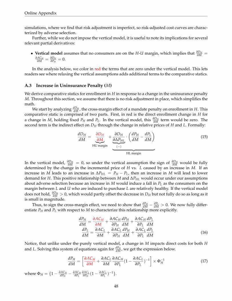
Online Appendix
simulations, where we find that risk adjustment is imperfect, so risk-adjusted cost curves are charac-terized by adverse selection.
Further, while we do not impose the vertical model, it is useful to note its implications for severalrelevant partial derivatives:
• Vertical model assumes that no consumers are on the H-U margin, which implies that ∂DH∂M =
∂ACH∂M = ∂DU
∂PH= 0.
In the analysis below, we color in red the terms that are zero under the vertical model. This letsreaders see where relaxing the vertical assumptions adds additional terms to the comparative statics.
A.3 Increase in Uninsurance Penalty (M)
We derive comparative statics for enrollment in H in response to a change in the uninsurance penaltyM. Throughout this section, we assume that there is no risk adjustment in place, which simplifies themath.
We start by analyzing dDHdM , the cross-margin effect of a mandate penalty on enrollment in H. This
comparative static is comprised of two parts. First, in red is the direct enrollment change in H fora change in M, holding fixed PH and PL. In the vertical model, this ∂DH
∂M term would be zero. Thesecond term is the indirect effect on DH through the change in relative prices of H and L. Formally:
dDH
dM=
∂DH
∂M︸ ︷︷ ︸HU margin
+∂DH
∂∆PHL︸ ︷︷ ︸(−)
·(
dPH
dM− dPL
dM
)︸ ︷︷ ︸
HL margin
(15)
In the vertical model, ∂DH∂M = 0, so under the vertical assumption the sign of ∂DH
∂M would be fullydetermined by the change in the incremental price of H vs. L caused by an increase in M. If anincrease in M leads to an increase in ∆PHL = PH − PL, then an increase in M will lead to lowerdemand for H. This positive relationship between M and ∆PHL would occur under our assumptionsabout adverse selection because an increase in M would induce a fall in PL as the consumers on themargin between L and U who are induced to purchase L are relatively healthy. If the vertical modeldoes not hold, ∂DH
∂M > 0, which would partly offset the decrease in DH but not fully do so as long as itis small in magnitude.
Thus, to sign the cross-margin effect, we need to show that dPHdM −
dPLdM > 0. We now fully differ-
entiate PH and PL with respect to M to characterize this relationship more explicitly.
dPH
dM=
∂ACH
∂M+
∂ACH
∂PH
dPH
dM+
∂ACH
∂PL
dPL
dMdPL
dM=
∂ACL
∂M+
∂ACL
∂PH
dPH
dM+
∂ACL
∂PL
dPL
dM(16)
Notice, that unlike under the purely vertical model, a change in M impacts direct costs for both Hand L. Solving this system of equations again for dPH
dM , we get the expression below.
dPH
dM=
[∂ACH
∂M+
∂ACL
∂M∂ACH
∂PL(1− ∂ACL
∂PL)−1]×Φ−1
H (17)
where ΦH = {1− ∂ACHdPH− ∂ACH
∂PL
∂ACL∂PH
(1− ∂ACL∂PL
)−1}.
48

Online Appendix
We now can sign dPHdM as follows:
dPH
dM=
∂ACH
∂M︸ ︷︷ ︸Ext. Margin Selection(≤0)
+∂ACL
∂M︸ ︷︷ ︸(−)
· ∂ACH
∂PL︸ ︷︷ ︸(−)
(1− ∂ACL
∂PL
)−1
︸ ︷︷ ︸(+)︸ ︷︷ ︸
Substitution to L (+)
× Φ−1
H︸︷︷︸(+)
(18)
and ΦH = (1− ∂ACH
dPH)︸ ︷︷ ︸
(+)
− ∂ACH
∂PL
∂ACL
∂PH︸ ︷︷ ︸(−)
(1− ∂ACL
∂PL)−1︸ ︷︷ ︸
(+)
> 0 , where all signs are determined by the
adverse selection and stability assumptions laid out above.Therefore, we can sign dPH
dM > 0 under the vertical model. The intuition is as we have alreadydescribed: the mandate penalty lowers PL, leading relatively healthy H consumers to leave H andsubstitute to L, which raises ACH and therefore PH. When the vertical model does not hold, extensivemargin selection of consumers on the HU margin into H ( ∂ACH
∂M < 0) pushes in the other direction.But as long as extensive margin substitution is not too large, the main effect of substitution to L willdominate.
We derive the expression for dPLdM in a similar way:
dPL
dM=
∂ACL
∂M︸ ︷︷ ︸Ext. Margin Selection(−)
+∂ACH
∂M︸ ︷︷ ︸(≤0)
· ∂ACL
∂PH︸ ︷︷ ︸(+)
(1− ∂ACH
∂PH
)−1
︸ ︷︷ ︸(+)︸ ︷︷ ︸
Substitution to H(≤0)
× Φ−1
L︸︷︷︸(+)
(19)
where ΦL = {1− ∂ACLdPL− ∂ACL
∂PH
∂ACH∂PL
(1− ∂ACH∂PH
)−1} > 0 as with ΦH above.
Thus, under the vertical model where ∂ACH∂M = 0, we can unambiguously say that PL falls with a
higher mandate penalty ( dPLdM < 0). This conclusion also holds when we relax the vertical model (as
shown by the negative substitution term), as any extensive margin substitution into H acts to lowerthe price of H, drawing the sickest consumers away from L and pushing L’s costs and price evenfurther down.
Returning now to dDHdM , we observe under the vertical model that
(dPHdM −
dPLdM
)< 0, which implies
that dDHdM > 0. In other words, the “unintended consequence" of decreasing enrollment in H should
always occur under the vertical model. When we relax the vertical model, this result will also holdas long substitution on the HU margin is not too large.
A.4 Increasing the Strength of Risk Adjustment (α)
We now consider in our more general model the effect of a small increase in the α parameter on theshare of the population that is uninsured. As in the previous section, we color in red the terms thatare zero under the vertical model. This lets readers see where relaxing the vertical assumptions addsadditional terms to the comparative statics.
49

Online Appendix
The change in the share of the uninsured population given a change in α is comprised of twoparts: changes in enrollment from the HU margin (in red) and LU margin (in black). Under thevertical model assumptions, the HU margin is not present.
dDU
dα=
∂DU
∂∆PHU︸ ︷︷ ︸≥0
d∆PHU
dα
︸ ︷︷ ︸HU margin
+∂DU
∂∆PLU︸ ︷︷ ︸(+)
d∆PLU
dα
︸ ︷︷ ︸LU margin
(20)
where ∆PHU = PH − S − M and ∆PLU = PL − S − M are the net prices of H and L relative touninsurance.
By the law of demand, ∂DU∂PH≥ 0, ∂DU
∂PL> 0. Under the vertical model, ∂DU
∂PH= 0, so the cross-margin
effect of risk adjustment on uninsurance is entirely determined by the sign of the LU margin. We nowconsider the impact of a change in α on ∆PHU and ∆PLU . The change in prices depends on the natureof subsidies. With subsidies linked to the price of L, ∆PLU (= PL − S−M) is fixed by construction.Therefore, the LU margin of substitution is shut down. In the vertical model, we will have dDU
dα = 0.Let us now consider the case where there is a fixed subsidy and therefore prices can be affected
by the level of transfers. We fully differentiate (14) and rearrange to get a system of equations. Theseare identical under both the horizontal and vertical model.
dPH
dα= T(.)︸︷︷︸
(+)
×
−1︸︷︷︸Direct(−)
+∂ACRA
H∂PL
(1− ∂ACRA
L∂PL
)−1
︸ ︷︷ ︸Substitution from L (−)
× (ΦRAH )−1 < 0
where ΦRAH ≡ 1− ∂ACRA
H∂PH
− ∂ACRAL
∂PH
∂ACRAH
∂PL(1− ∂ACRA
L∂PL
)−1. As in the mandate section above, this ΦRAH term
must be positive under the assumptions on stability and adverse selection we have made.The term in brackets is composed of two effects. First, there is a direct effect of stronger risk
adjustment transferring money to H, which tends to lower PH. Second, there is an indirect substitu-tion effect, arising from substitution of relatively healthy consumers on the margin between H and Lopting for H and lowering H’s average cost and thus its price. Thus, dPH
dα < 0 because both the directand indirect effects push PH down.
Doing the same for dPLdα gives
dPL
dα= T(.)︸︷︷︸
(+)
×
1︸︷︷︸Direct(+)
+
(−∂ACRA
L∂PH
)(1− ∂ACRA
H∂PH
)−1
︸ ︷︷ ︸Substitution to H (−)
× (ΦRAL )−1︸ ︷︷ ︸(+)
where ΦRAL ≡ 1− ∂ACRA
L∂PL− ∂ACRA
H∂PL
∂ACRAL
∂PH(1− ∂ACRA
H∂PH
)−1, which must be positive under the stability andadverse selection assumptions.
Here, the direct effect is positive because larger transfers take money from L, driving up the price
of L. However, the indirect substitution effect is negative—since ∂ACRAL
∂PH> 0 by adverse selection.
Intuitively, stronger risk adjustment transfers increase the price of L, causing consumers on the H-Lmargin to opt for H instead of L. These consumers are the highest-cost L enrollees, implying thattheir exit from L will lower L’s average cost and thus its price. Therefore, the indirect substitutioneffects will mute (or even fully offset) the direct effect of risk adjustment on PL. Because of this direct
50

Online Appendix
and indirect effect, it is ambiguous whether PL will increase or decrease, and in general, any changein PL will be smaller than one would expect from the direct effect alone.
Further, the question of whether the direct or indirect effect dominates depends on whether thesubstitution term is greater than or less than 1 in absolute value. If it is greater than 1, then the
substitution term will dominate. This will occur if ∂ACRAL
∂PH> 1− ∂ACRA
H∂PH
. This will tend to occur when
intensive margin adverse selection is very strong (even after risk adjustment) so that both ∂ACRAL
∂PHand
∂ACRAH
∂PHare large. Conversely, if adverse selection is weak, the direct effect will dominate.
This expression also tells us how the size of any cost advantage for L may affect the effects ofincreasing α. When L has no cost advantage over H (the cream-skimmer case), the only reason Lgets any demand is intensive margin adverse selection. When adverse selection is strong in thecream-skimmer case, L exists but the substitution effect is also large, muting the direct effect of riskadjustment. When adverse selection is weak in the cream-skimmer case, L fails to exist. Thus, it ismore likely that increasing α will have little or no (or possibly negative) effect on PL in the case whereL has no cost advantage than in the case where L has a cost advantage.
To summarize the case with fixed subsidies, dDUdα is ambiguous even under the vertical model
because we cannot theoretically sign the change in PL when when α increases. If the direct effectdominates, then PL will increase with α and uninsurance will rise under the vertical model. If thesubstitution to H dominates, then PL will fall and uninsurance will also fall.
When we relax the vertical assumptions, the potential for stronger risk adjustment to increaseuninsurance is further mitigated by the presence of the HU extensive margin. The term ∂DU
∂PH
dPHdα in
equation (20) will be positive. Because dPHdα < 0, consumers on the HU margin will tend to become
insured (in H) when risk adjustment is strengthened. This may offset any rise in uninsurance alongthe LU margin if PL rises, as more consumers leave uninsurance to buy H.
B Appendix: Graphical Analysis of Perfect Risk Adjustment
In this section, we illustrate how our graphical model can be used to show the effects of perfect riskadjustment on equilibrium prices and market shares. To simplify exposition, we assume that thecausal cost difference between H and L equals a constant value of δ for all consumer types s. Wedefine perfect risk adjustment as transfers such that the average cost in H net of risk adjustmentalways equals the average cost in L net of risk adjustment plus δ: RACH(P) = RACL(P) + δ. Underperfect risk adjustment, the average risk-adjusted cost in H and L does not depend on consumersorting between H and L. Instead, the average cost of both plans depends only on consumer sortingbetween insurance and uninsurance. If new healthy consumers join the market (buying the L plan),the risk transfers share the improved risk pool equally between H and L, maintaining the δ differencebetween their average costs. The important simplifying feature of perfect risk adjustment is that whenit comes to average costs, there is only one relevant margin of adjustment: the extensive margin.With imperfect risk adjustment, residual intensive margin selection that is not compensated by riskadjustment remains relevant, complicating the graphical analysis.
We depict the perfect risk adjustment case in Figure A1. Note that here we do not assume that Lis a pure cream-skimmer but instead that L has a cost advantage equal to δ. Risk adjustment affectsthe curves in a number of ways. First, as depicted in panel (b), risk adjustment causes the averagecost curve for L to shift upward and rotate slightly to make it parallel with the original, unadjustedaverage cost curve for H. This shift reflects the risk transfer away from L (and to H) that raises L’seffective costs. RACL(sLU) still slopes down because of extensive margin adverse selection, but it is
51

Online Appendix
Figure A1: Equilibrium under Perfect Risk Adjustment
(a) No Risk Adjustment
$
s
DL
ACH(sHL)𝑷𝑯𝒆
Buy L Unins
𝑷𝑳𝒆
𝑠𝐻𝐿𝑒 𝑃𝑒 𝑠𝐿𝑈
𝑒 (𝑃𝑒)
DH(𝑷𝑳𝒆)
WH
ACL(sLU ; sHL)
Buy H
(b) RA Shifts ACL Up, Lowers seLU
ACL(sLU ; sHL)
$
s
ACH(sHL)
WH
𝑷𝑯𝒆
RACL(sLU)
𝑷𝑳𝒆
𝑠𝐻𝐿𝑒 𝑃𝑒 𝑠𝐿𝑈
𝑒 (𝑃𝑒)
DL
𝑷𝑳𝒆
Ƹ𝑠𝐿𝑈𝑒 (𝑃𝑒)
Buy L UninsBuy H U instead of L
DH(𝑷𝑳𝒆)
(c) Lower seLU Pushes DH Up
ACL(sLU ; sHL)
$
s
ACH(sHL)
WH
𝑷𝑯𝒆
RACL(sLU)
𝑷𝑳𝒆
𝑠𝐻𝐿𝑒 𝑃𝑒 𝑠𝐿𝑈
𝑒 (𝑃𝑒)
DL
𝑷𝑳𝒆
Ƹ𝑠𝐿𝑈𝑒 (𝑃𝑒)
Buy L UninsBuy H U instead of L
DH(𝑷𝑳𝒆)
(d) RA Flattens ACH
ACL(sLU ; sHL)
$
s
ACH(sHL)
WH
𝑷𝑯𝒆
RACL(sLU)
𝑷𝑳𝒆
𝑠𝐻𝐿𝑒 𝑃𝑒 𝑠𝐿𝑈
𝑒 (𝑃𝑒)
DL
𝑷𝑳𝒆
Ƹ𝑠𝐿𝑈𝑒 (𝑃𝑒)
Buy L UninsBuy H U instead of L
RACH(sHL)
DH(𝑷𝑳𝒆)
Notes: Starting from equilibrium in panel (a) and introducing perfect risk adjustment in panel (c), perfect risk adjustmentshifts up the average cost of L from ACL(sLU) to RACL(sLU), reflecting the transfer away from L to H. Unlike ACL, therisk adjusted RACL only depends on the extensive margin SLU , not on the allocation across plans (sHL). The risk adjustedcurve RACL(sLU) intersects DL at a lower point, shifting out the extensive margin from se
LU to seLU . Next, in panel (c) we
see that this lower extensive margin-type seLU shifts up DH . Finally, in panel (d) we see that risk adjustment flattens the risk
adjusted average cost of H, RACH , which like RACL no longer varies depending on sorting between the two plans, sHL.
52

Online Appendix
now a fixed curve that does not depend on the price of H or sorting between H and L.37 The new,higher average cost curve for L, RACL implies a new, higher equilibrium price for L, Pe
L. This higherprice of L implies a new demand curve for H, shifted upward from the previous demand curve anddepicted in panel (c) of Figure A1. This higher demand curve for H reflects the fact that the higherprice of L makes L less attractive relative to H.
Panel (d) of Figure A1 illustrates the second direct effect of risk adjustment. For the H plan,risk adjustment causes the average cost curve, RACH(sHL), to be rotated downward relative to theunadjusted curve, ACH(sHL). RACH is now a flat line, since sorting between plans (i.e., the value ofsHL) does not affect average costs. The level of RACH equals ACH(sLU)—the average cost if the entirepopulation up to the extensive margin type sLU were to enroll in H.
Figure A2 shows how this shift in H’s average cost curve combines with the shift in H’s de-mand curve to produce a new lower equilibrium price of H, Pe
H and a higher quantity of consumersenrolling in H.
Figure A2: Equilibrium under Perfect Risk Adjustment
ACL(sLU ; sHL)
$
s
ACH(sHL)
WH
𝑷𝑯𝒆
RACL(sLU)
𝑷𝑳𝒆
𝑠𝐻𝐿𝑒 𝑃𝑒 𝑠𝐿𝑈
𝑒 (𝑃𝑒)
DH(𝑷𝑳𝒆)
DL
𝑷𝑳𝒆
Ƹ𝑠𝐿𝑈𝑒 (𝑃𝑒)
Buy L UninsBuy H U instead of L
RACH(sHL)
Ƹ𝑠𝐻𝐿𝑒 𝑃𝑒
𝑷𝑯𝒆
H instead of L
Unintended Consequence:
Risk adjustment shifts 𝐴𝐶𝐿 up,
raising 𝑃𝐿. Consumers choose L
instead of U.
Intended Consequence: Risk
adjustment rotates 𝐴𝐶𝐻 down,
higher 𝑃𝐿 shifts 𝐷𝐻 up, leading
to lower 𝑃𝐻. Consumers choose
H instead of L
Notes: Under perfect risk adjustment, the risk-adjusted average cost curve for H is completely flat for a given sLU . Equi-librium occurs at sHL and sLU values such that RACH intersects DH and RACL intersects DL.
Therefore, perfect risk adjustment has two effects. First, it narrows the average cost and thereforethe price gap between H and L, leading consumers to shift on the intensive margin towards the Hplan. This is the intended effect. Second, it pushes up the average cost and therefore the price of L.This results in some consumers who would have chosen L in the absence of risk adjustment insteadchoosing to be uninsured. This is the unintended, cross-margin consequence of risk adjustment. InSection 3 we also provide a graphical description of the welfare consequences of risk adjustment,
37One can show that RACL is parallel to the old ACH since it is capturing the overall average costs of everyone froms = 0 up to a given sLU cutoff.
53

Online Appendix
both perfect and imperfect.
C Appendix: Simulation Method Details
C.1 Constructing Demand and Cost Curves
As discussed in section 4, we draw on separate demand and cost estimates for both low-incomesubsidized consumers from Finkelstein, Hendren and Shepard (2019) (abbreviated "FHS") and high-income unsubsidized consumers from Hackmann, Kolstad and Kowalski (2015) (abbreviated "HKK").We describe how each respective paper produced its primitives as well as our modifications below.
C.1.1 Low-Income Demand and Costs: FHS (2019)
FHS Primitives
• Population: FHS estimate insurance demand in Massachusetts’ pre-ACA subsidized health in-surance exchange, known as “CommCare.” CommCare was an insurance exchange createdunder the state’s 2006 “Romneycare” reform to offer subsidized coverage to low-income non-elderly adults (below 300% of poverty) without access to other health insurance (from an em-ployer, Medicare, Medicaid, or another public program). This population was similar, thoughsomewhat poorer, than the subsidy-eligible population under the ACA.
• Market structure: CommCare participation was voluntary: consumers could choose to remainuninsured and pay a (small) penalty. As FHS show, a large portion of consumers (about 37%overall) choose the outside option of uninsurance, despite the penalty and large subsidies. TheCommCare market featured competing insurers, which offered plans with standardized (state-specified) cost sharing rules but which differed on their provider networks. In 2011, the mainyear that FHS estimate demand, the market featured a convenient vertical structure among thecompeting plans. Four insurers had relatively broad provider networks and charged nearlyidentical prices just below a binding price ceiling imposed by the exchange. One insurer (Celti-Care) had a smaller provider network and charged a lower price. FHS pool the four high-price,broad network plans into a single "H option"—technically defined as each consumer’s preferredchoice among the four plans—and treat CeltiCare as a vertically lower-ranked "L option." FHSpresent evidence that this vertical ranking is a reasonable characterization of the CommCaremarket in 2011.
• FHS Estimation: To estimate demand and costs, FHS use a regression discontinuity designleveraging discontinuous cutoffs in subsidy amounts based on household income. Becausesubsidies vary across income thresholds, there is exogenous net price variation that can trans-parently identify demand and cost curves with minimal parametric assumptions. FHS lever-age discontinuous changes in net-of-subsidy premiums at 150% FPL, 200% FPL, and 250% FPLarising from CommCare’s subsidy rules. They estimate consumer willingness-to-pay for thelowest-cost plan (L) and incremental consumer willingness-to-pay for the other plans (H) rela-tive to that plan.38 This method provides estimates of the demand curve for particular rangesof s. The same variation is used to estimate ACH(s) and CH(s), the average and marginalcost curves for H. Our goal is not to innovate on these estimates but rather to apply them asprimitives in our policy simulations to understand the empirical relevance of our conceptualframework.
38Because the base subsidy for L and the incremental subsidy for H change discontinuously at the income cutoffs, thereis exogenous variation in both the price of L and the incremental price of H.
54

Online Appendix
Our Modifications to FHS Primitives
• Extrapolating to extremes of s distribution: The FHS strategy provides four points of the WL(s)curve and four points of the WHL(s) = WH(s) −WL(s) curve. As shown in Figure 10 fromFHS, for the WL curve these points span from s = 0.36 to s = 0.94 and for the WHL curvethese points span from s = 0.31 to s = 0.80. Because our model allows for the possibility ofzero enrollment in either L or H or both, we need to modify the curves, extrapolating to thefull range of consumers, s ∈ [0, 1]. We start by extrapolating linearly, and then we “enhance”demand for H among the highest WTP consumers, as we view this as more realistic than a linearextrapolation. (We explore the sensitivity of our empirical results to alternative assumptionsabout this WTP enhancement in Appendix D.4.2) We then smooth the enhanced demand curvesto eliminate artificial kinks produced by the estimation and extrapolation.
(1) Linear demand: For the linear demand curves, we extrapolate the curves linearly to s = 0and s = 1.0. Call these curves W lin
L (s) and W linH (s), with incremental WTP defined as W lin
HL =W lin
H −W linL (s).
(2) Enhanced demand: For the enhanced demand curves(Wenh
L (s) and WenhH (s)
), we inflate
consumers’ relative demand for H vs. L in the extrapolated region, relative to a linear extrap-olation. We implement enhanced demand in an ad hoc but transparent way: We first generateWenh
L (s) = W linL (s) for all s. For all s >= 0.31 (the boundary of the "in-sample" region of
WHL(s)), we likewise set WenhHL (s) = W lin
HL(s). For s = 0, we set WenhHL (s = 0) = 3W lin
HL(s = 0), sothat the maximum enhanced incremental willingness-to-pay is three times the value suggestedby the primitives. We then linearly connect the incremental willingness to pay between s=0 ands=0.31, setting Wenh
HL (s < 0.31) = W linHL (s) + 3× (0.31−s)
0.31 ×W linHL (0) so that the enhanced curve is
equal to the linear curve for s >= 0.31, equal to three times the linear curve at s = 0, and linearbetween s = 0.31 and s = 0. This approach assumes that there exists a group of (relatively sick)consumers who exhibit very strong demand for H relative to L, which seems likely to be truein the real world. Thus,
WenhHL (s) =
{W lin
HL (s) for s ∈ [0.31, 1]W lin
HL (s) + 3× (0.31−s)0.31 ×W lin
HL (0) for s ∈ [0, 0.31)(21)
and
WenhH (s) = W lin
L (s) + WenhHL (s) (22)
Both the linear and the enhanced WTP curves are shown in the top panel of Figure A3.
• Cost of L plan: We need to produce estimates of CL(s) to complete the model. FHS providesuggestive evidence that CL(s) is quite similar to CH(s)—i.e., that for a given enrollee, L doesnot save money relative to H. We conducted further analyses to provide additional evidence onthis question (leveraging entry of the L plan in some areas but not others, leveraging additionalprice variation for L vs. H, etc.), consistently finding a lack of evidence of any cost advantagefor L among the enrollees marginal to these sources of variation. While L may indeed be a purecream-skimmer in this setting, the assumption that CH(s) = CL(s) for all s seems unlikely tohold in many other settings. Thus, we consider both the setting where L has a 15% cost advan-tage so that CL(s) = 0.85CH(s) and the setting where, consistent with the empirical evidence, Lis a pure cream-skimmer, i.e. CL(s) = CH(s).
• Smoothing primitives: Because they were estimated using a regression discontinuity design,the primitives above all have discrete “kink points" at which the slope of the curve with respect
55
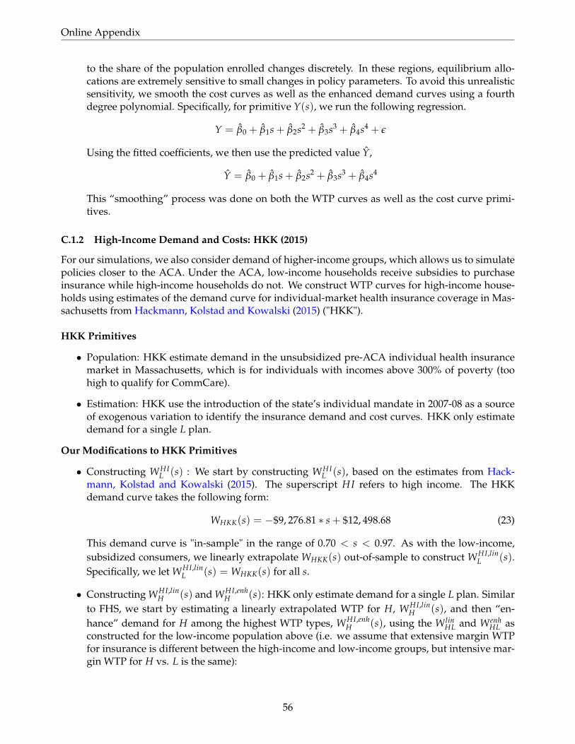
Online Appendix
to the share of the population enrolled changes discretely. In these regions, equilibrium allo-cations are extremely sensitive to small changes in policy parameters. To avoid this unrealisticsensitivity, we smooth the cost curves as well as the enhanced demand curves using a fourthdegree polynomial. Specifically, for primitive Y(s), we run the following regression.
Y = β0 + β1s + β2s2 + β3s3 + β4s4 + ε
Using the fitted coefficients, we then use the predicted value Y,
Y = β0 + β1s + β2s2 + β3s3 + β4s4
This “smoothing” process was done on both the WTP curves as well as the cost curve primi-tives.
C.1.2 High-Income Demand and Costs: HKK (2015)
For our simulations, we also consider demand of higher-income groups, which allows us to simulatepolicies closer to the ACA. Under the ACA, low-income households receive subsidies to purchaseinsurance while high-income households do not. We construct WTP curves for high-income house-holds using estimates of the demand curve for individual-market health insurance coverage in Mas-sachusetts from Hackmann, Kolstad and Kowalski (2015) ("HKK").
HKK Primitives
• Population: HKK estimate demand in the unsubsidized pre-ACA individual health insurancemarket in Massachusetts, which is for individuals with incomes above 300% of poverty (toohigh to qualify for CommCare).
• Estimation: HKK use the introduction of the state’s individual mandate in 2007-08 as a sourceof exogenous variation to identify the insurance demand and cost curves. HKK only estimatedemand for a single L plan.
Our Modifications to HKK Primitives
• Constructing WHIL (s) : We start by constructing WHI
L (s), based on the estimates from Hack-mann, Kolstad and Kowalski (2015). The superscript HI refers to high income. The HKKdemand curve takes the following form:
WHKK(s) = −$9, 276.81 ∗ s + $12, 498.68 (23)
This demand curve is "in-sample" in the range of 0.70 < s < 0.97. As with the low-income,subsidized consumers, we linearly extrapolate WHKK(s) out-of-sample to construct WHI,lin
L (s).Specifically, we let WHI,lin
L (s) = WHKK(s) for all s.
• Constructing WHI,linH (s) and WHI,enh
H (s): HKK only estimate demand for a single L plan. Similarto FHS, we start by estimating a linearly extrapolated WTP for H, WHI,lin
H (s), and then “en-hance” demand for H among the highest WTP types, WHI,enh
H (s), using the W linHL and Wenh
HL asconstructed for the low-income population above (i.e. we assume that extensive margin WTPfor insurance is different between the high-income and low-income groups, but intensive mar-gin WTP for H vs. L is the same):
56

Online Appendix
WHI,linH (s) = WHI
L + W linHL(s)
WHI,enhH (s) = WHI
L + WenhHL (s)
• Constructing CHIL (s), CHI
H (s): We assume that the cost curves for this group are equivalent tothe cost curves of the subsidized population, Thus,
CHIH (s) = CH(s)
CHIL (s) = CL(s)
where CH(s) is drawn from FHS and CL(s) is the curve as constructed in the previous section.We note that these assumptions imply that the high-income consumers have a level shift in WTPwith no difference in the extent of intensive or extensive margin selection from the low-incomeconsumers.
• Smoothing primitives: Similar to above, we also smooth primitives.
We thus have two demand systems: one for low-income consumers and one for high-incomeconsumers. Both exhibit WTP for H that is “enhanced” for the highest WTP types beyond what asimple linear extrapolation would imply. We combine these systems to form one set of demand andcost curves, by assuming that 60% of the market is low-income and 40% of the market is high-income,consistent with the population in the ACA Health Insurance Marketplaces.
57
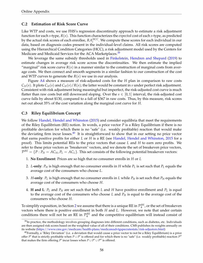
Online Appendix
C.2 Estimation of Risk Score Curve
Like WTP and costs, we use FHS’s regression discontinuity approach to estimate a risk adjustmentfunction for each s-type, R(s). This function characterizes the expected cost of each s-type, as predictedby the actual risk scores of each enrollee, RAHCC
i . We compute these scores for each individual in ourdata, based on diagnosis codes present in the individual-level claims. All risk scores are computedusing the Hierarchical Condition Categories (HCC), a risk adjustment model used by the Centers forMedicare and Medicaid Services for the ACA Marketplaces.39
We leverage the same subsidy thresholds used in Finkelstein, Hendren and Shepard (2019) toestimate changes in average risk score across the discontinuities. We then estimate the implied“marginal” risk score curve R(s) in a manner similar to the construction of marginal costs from aver-age costs. We then connect and smooth segments in a similar fashion to our construction of the costand WTP curves to generate the R(s) we use in our analysis.
Figure A4 shows a measure of risk-adjusted costs for the H plan in comparison to raw costsCH(s). It plots CH(s) and CH(s)/R(s); the latter would be constant in s under perfect risk adjustment.Consistent with risk adjustment being meaningful but imperfect, the risk-adjusted cost curve is muchflatter than raw costs but still downward sloping. Over the s ∈ [0, 1] interval, the risk-adjusted costcurve falls by about $130, compared to a fall of $367 in raw costs. Thus, by this measure, risk scoresnet out about 35% of the cost variation along the marginal cost curve for H.
C.3 Riley Equilibrium Concept
We follow Handel, Hendel and Whinston (2015) and consider equilibria that meet the requirementsof the Riley Equilibrium (RE) notion. In words, a price vector P is a Riley Equilibrium if there is noprofitable deviation for which there is no "safe" (i.e. weakly profitable) reaction that would makethe deviating firm incur losses.40 It is straightforward to show that in our setting no price vectorthat earns positive profits for either L or H is a RE (see Handel, Hendel and Whinston, 2015 for aproof). This limits potential REs to the price vectors that cause L and H to earn zero profits. Werefer to these price vectors as "breakeven" vectors, and we denote the set of breakeven price vectors,PBE = {P : PH = ACH, PL = ACL}. This set consists of the following potential breakeven vectors:
1. No Enrollment: Prices are so high that no consumer enrolls in H or L
2. L-only: PH is high enough that no consumer enrolls in H while PL is set such that PL equals theaverage cost of the consumers who choose L.
3. H-only: PL is high enough that no consumer enrolls in L while PH is set such that PH equals theaverage cost of the consumers who choose H.
4. H and L: PL and PH are set such that both L and H have positive enrollment and PL is equalto the average cost of the consumers who choose L and PH is equal to the average cost of theconsumers who choose H.
To simplify exposition, in Section 2 we assume that there is a unique RE inPBE4 , or the set of breakeven
vectors where there is positive enrollment in both H and L. However, we note that under certainconditions there will not be an RE in PBE
4 and the competitive equilibrium will instead consist of
39In practice, the methodology involves grouping diagnoses into different conditions, such as diabetes, etc. Individualsare then assigned risk scores based on the weighted value of all of their conditions. CMS publishes its weights annually onits website (https://www.cms.gov/medicare/health-plans/medicareadvtgspecratestats/risk-adjustors.html)
40Formally, a "Riley Deviation" (i.e. a deviation that would cause a price vector to not be a Riley Equilibrium) is a priceoffer P′ that is strictly profitable when P ∪ P′ is offered and for which there is no "safe" (i.e. weakly profitable) reaction P′′
that makes the firm offering P′ incur losses when P ∪ P′ ∪ P′′ is offered.
58

Online Appendix
Figure A3: WTP Curves for H and L
(a) Low-Income
(b) High-Income
Notes: Figure shows WTP Curves for H and L, WH(s) and WL(s). The top panel shows curves for low-income group whichcome from (Finkelstein, Hendren and Shepard, 2019). The bottom panel shows curves for high-income group which comefrom (Hackmann, Kolstad and Kowalski, 2015). Linear curves extrapolate linearly over the out-of-sample range [0,0.31].Modified (i.e. "enhanced") curves assume that the lowest s-types have very high incremental WTP for H.
59
Online Appendix
Figure A4: Raw Costs (CH) versus Risk-Adjusted Costs
Notes: Figure shows raw CH (black, continuous line) and risk-score normalized CH (blue, dashed). While the risk score isable to flatten out the cost curve somewhat, not all risk is captured by the score, leaving some slope.
positive enrollment in only one or neither of the two plan options. We allow for these possibilitiesin the empirical portion of the paper.41 Given the assumption that in equilibrium there is positiveenrollment in H and L, we have the familiar equilibrium condition that prices are set equal to averagecosts:
PH = ACH (P)PL = ACL (P) (24)
We use this expression to define equilibrium throughout Section 2.
C.4 Reaction Function Approach to Finding Equilibrium
Evaluating demand, profits: For each uninsurance penalty, risk adjustment strength, L-plan costadvantage, and subsidy type setting, we find the equilibrium PL and PH pair using the followinggrid-search method. We construct a grid of PL, PH price combinations, with H on the vertical axisand L on the horizontal axis. For most simulations, we use a coarse grid with $1 units. For each pair,we evaluate H and L profits using the demand, cost, and risk-adjustment equations as detailed inthe body of the paper. For insurance types H, L and uninsurance U we evaluate demand by find-ing the “indifference points"–the first and the last points in the s distribution such that each typeof insurance’s enrollment conditions are satisfied. Because of the vertical model, we can attributeall intermediate points of the s distribution between these indifference points to a given plan. If no
41Handel, Hendel and Whinston, 2015 show that there is a unique RE in the setting where there is no outside option.With an outside option, their definition of a Riley Equilibrium requires a slight modification in order to achieve unique-ness. Specifically, instead of requiring the deviation to be strictly profitable, we require the deviation to be weakly profitablebut also to achieve positive enrollment for the deviating plan. In the empirical exercise below, we use this definition to findthe competitive equilibrium for each counterfactual simulation.
60

Online Appendix
points on the s vector satisfy the plan’s enrollment conditions, the plan has zero enrollment. We haveindifference points sHL, sLU if both H and L have non-zero enrollment and sHU , sLU if L or H has zeroenrollment, respectively. If there is non-zero demand for both H and L, we calculate the average riskof those enrolled in each plan and construct transfers from the less risky plan to the more risky plan,per the ACA risk adjustment formula (see equation 9). (In some counterfactual policy simulations,the transfer is multiplied by α.) Finally, average costs are calculated for each plan with non-zeroenrollment. The function returns the H, L profit grids ΠH, ΠL with which we can then evaluate equi-librium.
Finding equilibrium: For a given grid coarseness, we set a tolerance value T equal to the incre-ment between grid points. A plan is considered to have zero profits if its profits are between −T andT. Potential equilibria are all price pairs where (1) only H exists and is making zero profits (2) only Lexists and is making zero profits (3) both H and L exist and are both making zero profits. Given thecoarseness of the grid, there are usually multiple potential equibria of each type. We use the follow-ing process to refine this set down to the final equilibrium point.
• Single plan equilibria: First, we refine our L−only and H−only equilibria. For the remainderof this paragraph, we will refer to the potential L−only equilibria, but the methodology alsoapplies to potential H−only equilibria. Given the curved nature of the primitives, for somesettings, especially those where L has a large cost advantage, there are multiple L−only pricesPL−only
L that are potential L−only equilibria. For each of these PL−onlyL , we evaluate a single
point (PL−onlyL , PH). For a given L−only equilibrium price PL−only
L , there are typically a set ofPH > Pmin
H that satisfy the conditions (1) L makes zero profit and (2) H has zero enrollment. Tocut down on the number of potential equilibria we must evaluate, for each PL−only
L , we evaluateonly the pair that contains the smallest PH: (Pmin
H , PL−onlyL ). For each potential PL−only
L , we needonly to evaluate this minimum price since any potential H deviations from (Pmin
H , PL) wouldalso be deviations from (PH, PL), PH > Pmin. Once a set of potential L−only equilibria priceshave been refined to unique (Ponly
L , PH) pairs, we then evaluate each PL−onlyL to determine if
it is a Riley Equilibrium. We begin with the minimum PL−onlyL . The Riley Equilibrium code
involves three nested loops. First, the outer loop evaluates each grid point ΠH(PL−onlyL , P′H),
P′H < PH to identify potential H-deviations where ΠH(PL−onlyL , P′H) > T. If no such potential H-
deviations are found, (PL−onlyL , PH) is considered a RE. If a potential H-deviation is found, the
second loop is called. This loop evaluates each grid point (P′L, P′H), P′L < PL to identify potentialL-retaliations where ΠL(P′L, P′H) > −T, ΠH(P′L, P′H) < −T. If no such potential retaliationsare found for a given potential H-deviation, then (PL−only
L , PH) is not a Riley Equilibrium. If apotential retaliation is found, a third loop is activated to evaluate if there is any point (P′L, P′′H),P′′H < P′H that makes a given retaliation “unsafe" where unsafe is defined as ΠL < −T. If no such“unsafe" point exists, then the retaliation point is safe and the potential deviation would notsucceed. The next potential deviation point for this PL−only
L is then evaluated. If no retaliation-proof deviation exists for a given (Ponly
L , PH), then the point is a RE. If a deviation does exist,the next larger PL−only
L is tested.
• H-L equilibria: Because of the coarseness of the grid, there are usually multiple connectedpoints where both H and L have enrollees and are making zero profits. We pick the point withthe lowest PL to evaluate. For each potential HL equilibrium, we test if any single-plan devia-tions exist. This consists of checking whether any H−deviations or L−deviations exist, using
61

Online Appendix
the same set of RE loops described in the previous paragraph. If either an H deviation or an Ldeviation is found, the HL equilibrium is not an RE.
D Appendix: Additional Simulation Results
D.1 Simulation Results for Mandate/Uninsurance Penalty
Tables A1 and A2 Show additional outcomes for the mandate/uninsurance penalty simulations dis-cussed in Section 5 and shown in Figure 9. In all cases, the welfare measure represents the socialsurplus under the particular policy setting as a percent of the difference between minimum possiblesocial surplus and maximum possible social surplus achieved.
Table A1: Varying Mandate Penalty
(a) ACA-like subsidy, L cream-skimmer
mandate 0 15 30 45 60price H 382 374 371 360 349price L 352 344 337 325 313share H .42 .42 .3 .26 .23share L .31 .37 .55 .67 .77share U .27 .21 .15 .069 0subsidy 297 289 282 270 258welfare .91 .76 .49 .24 0
(b) Fixed $275, L cream-skimmer
mandate 0 15 30 45 60price H 387 381 373 349 349price L 357 351 341 313 313share H .42 .42 .37 .23 .23share L .24 .3 .44 .77 .77share U .35 .28 .19 0 0subsidy 275 275 275 275 275welfare .93 .79 .56 0 0
(c) ACA-like subsidy, L cost advantage
mandate 0 15 30 45 60price H 414 409 404 399 .price L 307 300 292 283 273share H .021 .017 .013 .0065 0share L .73 .79 .86 .93 1share U .25 .19 .13 .067 0subsidy 252 245 237 228 218welfare .95 .75 .52 .27 0
(d) Fixed $250 , L cost advantage
mandate 0 15 30 45 60price H 415 404 . . .price L 307 294 273 273 273share H .019 .016 0 0 0share L .73 .84 1 1 1share U .26 .15 0 0 0subsidy 250 250 250 250 250welfare .27 .16 0 0 0
Notes: Table A1 contains equilibrium prices, market shares, subsidy levels and relative welfare under varying levels ofmandate penalties. Panels (a) and (b) are results for when L is a cream-skimmer (∆CHL = 0) while panels (c) and (d) arefor when L has a 15% cost advantage. In panels (a) and (c), the market has a price-linked subsidy while in panels (b) and(d), the market has a fixed subsidy. Relative welfare is calculated as wel f are−min(wel f are)
max(wel f are)−min(wel f are) where max and min are takenover integer mandate penalty values 0 to 60 under the panel’s same L cost advantage, subsidy scheme.
D.2 Simulations of Benefit Regulation
Tables A3 and A4 characterize equilibrium results with and without an L-plan offered when the L-plan is a pure cream-skimmer and when L has a 15% cost advantage. For a given setting, the welfareloss is reported in dollars and represents loss relative to welfare under the optimal allocation.
62

Online Appendix
Table A2: Varying Risk Adjustment (α)
(a) ACA-like subsidy, L cream-skimmer
α 0 .5 1 1.5 2price H . 437 382 362 362price L 372 362 352 . .share H 0 .082 .42 .78 .78share L .72 .64 .31 0 0share U .28 .28 .27 .22 .22subsidy 317 307 297 307 307welfare .46 .59 .91 .91 .91
(b) Fixed $275, L cream-skimmer
α 0 .5 1 1.5 2price H 495 438 387 377 377price L 381 369 357 . .share H .0095 .097 .42 .66 .66share L .57 .52 .24 0 0share U .42 .38 .35 .34 .34subsidy 275 275 275 275 275welfare .68 .73 .93 1 1
(c) ACA-like subsidy, L cost advantage
α 0 .5 1 1.5 2price H . . 414 361 362price L 308 308 307 313 .share H 0 0 .021 .16 .78share L .75 .75 .73 .59 0share U .25 .25 .25 .25 .22subsidy 253 253 252 258 307welfare .93 .93 .95 .99 .58
(d) Fixed $250, L cost advantage
α 0 .5 1 1.5 2price H . . 415 365 381price L 309 309 307 316 .share H 0 0 .019 .16 .6share L .74 .74 .73 .56 0share U .26 .26 .26 .29 .4subsidy 250 250 250 250 250welfare .24 .24 .27 .48 1
Notes: Table A2 contains equilibrium prices, market shares, subsidy levels and relative welfare under varying strengths ofrisk adjustment α. Panels (a) and (b) are results for when L is a cream-skimmer (∆C = 0) while panels (c) and (d) are forwhen L has a 15% cost advantage. In panels (a) and (c), the market has a price-linked subsidy while in panels (b) and (d),the market has a fixed subsidy. relative welfare is reported as wel f are−min(wel f are)
max(wel f are)−min(wel f are) where max and min are taken overinteger mandate penalty values 0 to 60 under the panel’s same L cost advantage, subsidy scheme.
The results indicate that for the ACA-like price-linked subsidies, removing L from the choice setalways (weakly) improves welfare. This is because removing L results in a higher subsidy and morepeople entering the market. In the fixed subsidy cases, we find that removing L often causes both anincrease in H’s market share and an increase in the uninsurance rate (especially when L has a 15%cost advantage). However, we find that in all cases, benefit regulation improves welfare, implyingthat the welfare losses from more people being uninsured are more than offset by welfare gains frommore people enrolling in H.
D.3 Additional Welfare Results from Simulations
D.3.1 Graphical Illustration of Welfare Consequences of an Uninsurance Penalty
In this appendix we show how to estimate the welfare consequences of an uninsurance penalty withour graphical model. This exercise corresponds to the similar exercise analyzing the welfare conse-quences of risk adjustment in the main text. Panel (a) of Figure A5 plots the empirical analogs to ourwelfare figure from Section 2 for the case where L is a pure cream-skimmer. Instead of plotting CL,we plot CNet
L = CL − CU , as in Eq. (8) to account for the fact that CU 6= 0. We indicate the equilibriums cutoffs for the baseline ACA setting, where subsidies are linked to the price of the lowest-pricedplan, α = 1, and there is no uninsurance penalty. The intensive margin equilibrium cutoff is se
HLand the extensive margin cutoff is se
LU . Thus, consumers with s < seHL enroll in H, consumers with
63
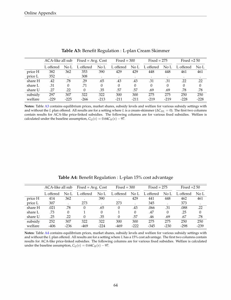
Online Appendix
Table A3: Benefit Regulation : L-plan Cream Skimmer
ACA-like all sub Fixed = Avg. Cost Fixed = 300 Fixed = 275 Fixed =2 50
L offered No L L offered No L L offered No L L offered No L L offered No Lprice H 382 362 353 390 429 429 448 448 461 461price L 352 . 308 . . . . . . .share H .42 .78 .29 .65 .43 .43 .31 .31 .22 .22share L .31 0 .71 0 0 0 0 0 0 0share U .27 .22 0 .35 .57 .57 .69 .69 .78 .78subsidy 297 307 322 322 300 300 275 275 250 250welfare -229 -225 -266 -213 -211 -211 -219 -219 -228 -228
Notes: Table A3 contains equilibrium prices, market shares, subsidy levels and welfare for various subsidy settings withand without the L plan offered. All results are for a setting where L is a cream-skimmer (∆CHL = 0). The first two columnscontain results for ACA-like price-linked subsidies. The following columns are for various fixed subsidies. Welfare iscalculated under the baseline assumption, CU(s) = 0.64CH(s)− 97.
Table A4: Benefit Regulation : L-plan 15% cost advantage
ACA-like all sub Fixed = Avg. Cost Fixed = 300 Fixed = 275 Fixed =2 50
L offered No L L offered No L L offered No L L offered No L L offered No Lprice H 414 362 . 390 . 429 441 448 462 461price L 307 . 273 . 273 . 345 . 373 .share H .021 .78 0 .65 0 .43 .066 .31 .088 .22share L .73 0 1 0 1 0 .47 0 .25 0share U .25 .22 0 .35 0 .57 .46 .69 .67 .78subsidy 252 307 322 322 300 300 275 275 250 250welfare -406 -236 -469 -224 -469 -222 -345 -230 -298 -239
Notes: Table A4 contains equilibrium prices, market shares, subsidy levels and welfare for various subsidy settings withand without the L plan offered. All results are for a setting where L has a 15% cost advantage. The first two columns containresults for ACA-like price-linked subsidies. The following columns are for various fixed subsidies. Welfare is calculatedunder the baseline assumption, CU(s) = 0.64CH(s)− 97.
64

Online Appendix
seHL < s < se
LU enroll in L, and consumers with s > seLU remain uninsured.
Figure A5: Empirical Estimates of Foregone Surplus
(a) Baseline Foregone Surplus (b) Impose $60 Penalty
Notes: Panels (a) and (b) show welfare losses under ACA-like subsidies relative to efficient sorting, when L is a cream-skimmer and when L has a 15% cost advantage over H, respectively. In both settings, 60% of the population is low-income and 40% of the population is high-income, so WTP curves are weighted sums of both types. Efficient cutoffs areindicated with a * while equilibrium outcomes are denoted with an e superscript. For both panel (a) and (b), we assumeCU(s) = 0.64CH(s)− 97.
It is apparent that, from a social surplus perspective, no consumer should be in L because WH −(CH − CL) is everywhere above WL. This is because L is a pure cream-skimmer: All consumers valueH more than L and L has no cost advantage over H. In addition, in this setting some consumers (thosewith s > s∗HU) should not be insured at all. These consumers do not value either H or L more thanthe (net) cost of enrolling them, making it inefficient for them to be insured. In the figure, we depictthe foregone surplus in the baseline ACA setting with shaded areas. The foregone intensive marginsurplus in panel (a) (lost surplus due to consumers choosing L instead of H) is described by the areabetween WNet
H and WL for the consumers not enrolled in H, ACDB. This area represents a welfare lossof $41.92. The foregone extensive margin surplus (lost surplus due to consumers choosing U insteadof L) is given by the area between WL and CNet
L for the consumers who are not enrolled in insurancebut should be, EDF. This area represents a welfare loss of $16.58. The total foregone surplus in thebaseline ACA setting in panel (a) of Figure A5 is $58.50.
Panel (b) of Figure A5 shows how we estimate the welfare consequences of adding an uninsur-ance penalty of $60 per month to the baseline case from Panel (a). Recall from the top-left panelof Figure 9 that the imposition of a $60 mandate (1) induces all previously uninsured consumers topurchase insurance and (2) causes a shift of 19% of the market from H to L. Effect (1) is the intendedconsequence of the penalty, and it implies both welfare gains and losses. Welfare gains occur amongthose consumers who value L more than CNet
L = CL − CU and who newly enroll in L (green welfaretriangle EFG). Welfare losses occur among those consumers who value L less than CNet
L and whonewly enroll in L (red welfare triangle GHI). Together, the intended consequence of the penalty,inducing all consumers to purchase insurance, implies a net welfare gain of $16.59. Effect (2) is theunintended consequence of the penalty, shifting consumers from H to L. Here, it implies a welfareloss of $57.83, which arises because H and L have similar costs but all consumers value H more than
65
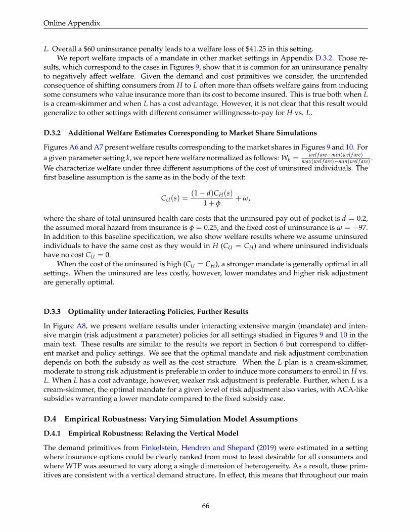
Online Appendix
L. Overall a $60 uninsurance penalty leads to a welfare loss of $41.25 in this setting.We report welfare impacts of a mandate in other market settings in Appendix D.3.2. Those re-
sults, which correspond to the cases in Figures 9, show that it is common for an uninsurance penaltyto negatively affect welfare. Given the demand and cost primitives we consider, the unintendedconsequence of shifting consumers from H to L often more than offsets welfare gains from inducingsome consumers who value insurance more than its cost to become insured. This is true both when Lis a cream-skimmer and when L has a cost advantage. However, it is not clear that this result wouldgeneralize to other settings with different consumer willingness-to-pay for H vs. L.
D.3.2 Additional Welfare Estimates Corresponding to Market Share Simulations
Figures A6 and A7 present welfare results corresponding to the market shares in Figures 9 and 10. Fora given parameter setting k, we report here welfare normalized as follows: Wk =
wel f are−min(wel f are)max(wel f are)−min(wel f are) .
We characterize welfare under three different assumptions of the cost of uninsured individuals. Thefirst baseline assumption is the same as in the body of the text:
CU(s) =(1− d)CH(s)
1 + φ+ ω,
where the share of total uninsured health care costs that the uninsured pay out of pocket is d = 0.2,the assumed moral hazard from insurance is φ = 0.25, and the fixed cost of uninsurance is ω = −97.In addition to this baseline specification, we also show welfare results where we assume uninsuredindividuals to have the same cost as they would in H (CU = CH) and where uninsured individualshave no cost CU = 0.
When the cost of the uninsured is high (CU = CH), a stronger mandate is generally optimal in allsettings. When the uninsured are less costly, however, lower mandates and higher risk adjustmentare generally optimal.
D.3.3 Optimality under Interacting Policies, Further Results
In Figure A8, we present welfare results under interacting extensive margin (mandate) and inten-sive margin (risk adjustment α parameter) policies for all settings studied in Figures 9 and 10 in themain text. These results are similar to the results we report in Section 6 but correspond to differ-ent market and policy settings. We see that the optimal mandate and risk adjustment combinationdepends on both the subsidy as well as the cost structure. When the L plan is a cream-skimmer,moderate to strong risk adjustment is preferable in order to induce more consumers to enroll in H vs.L. When L has a cost advantage, however, weaker risk adjustment is preferable. Further, when L is acream-skimmer, the optimal mandate for a given level of risk adjustment also varies, with ACA-likesubsidies warranting a lower mandate compared to the fixed subsidy case.
D.4 Empirical Robustness: Varying Simulation Model Assumptions
D.4.1 Empirical Robustness: Relaxing the Vertical Model
The demand primitives from Finkelstein, Hendren and Shepard (2019) were estimated in a settingwhere insurance options could be clearly ranked from most to least desirable for all consumers andwhere WTP was assumed to vary along a single dimension of heterogeneity. As a result, these prim-itives are consistent with a vertical demand structure. In effect, this means that throughout our main
66

Online Appendix
Figure A6: Welfare with Varying Mandate Penalty (M)
(a) ACA-like subsidy, L cream-skimmer (b) Fixed $275 subsidy, L cream-skimmer
(c) ACA-like subsidy, L cost advantage (d) Fixed $250 subsidy, L cost advantage
Notes: Figure A6 depicts equilibrium relative welfare under varying levels of the mandate penalty. The simulations are thesame as in figure 9. Panels (a) and (b) are results for when L is a cream-skimmer (∆CHL = 0) while panels (c) and (d) are forwhen L has a 15% cost advantage. In panels (a) and (c), the market has a price-linked subsidy while in panels (b) and (d),the market has a fixed subsidy. For each set of simulations, we present relative welfare under three different assumptionsabout the social cost of uninsurance. Relative welfare is calculated as wel f are−min(wel f are)
max(wel f are)−min(wel f are) where max and min are takenover the possible mandate penalties within a set of simulations and CU assumptions.
simulations, individuals are only on the margin between H and L or L and U, never on the mar-gin between H and U (except in cases where the market “upravels” and nobody chooses L). Asthe theoretical analysis in Appendix A shows, allowing for an HU substitution margin that wouldbe present with horizontal differentiation adds additional terms to the comparative statics definingcross-margin policy effects.
We can investigate how robust our empirical results are to the vertical model by assuming someportion of the population does not value L at all and is thus solely on the margin between H and U.To do this, we perform the following exercise:
Simulation modifications
• From our standard population comprising 60% subsidized low income types and 40% unsub-sidized high income types, we assume γ percent of each type do not value L so that they mayonly choose between H and U
• We assume that this γ portion has the standard WH(s) and WHIH (s) curves and same s distribu-
tion as in our baseline simulations
67

Online Appendix
Figure A7: Welfare with Varying Strength of Risk Adjustment (α)
(a) ACA-like subsidy, L cream-skimmer (b) Fixed $ 275 subsidy, L cream-skimmer
(c) ACA-like subsidy, L cost advantage (d) Fixed $ 250 subsidy, L cost advantage
Notes: Figure A6 depicts equilibrium relative welfare under varying strengths of risk adjustment α. The simulations arethe same as in figure 10. Panels (a) and (b) are results for when L is a cream-skimmer (∆CHL = 0) while panels (c) and(d) are for when L has a 15% cost advantage. In panels (a) and (c), the market has a price-linked subsidy while in panels(b) and (d), the market has a fixed subsidy. For each set of simulations, we present relative welfare under three differentassumptions about the social cost of uninsurance. Relative welfare is calculated as wel f are−min(wel f are)
max(wel f are)−min(wel f are) where max andmin are taken over the possible α values within a set of simulations and CU assumptions.
• The remaining 1− γ portion of the population has the standard demand primitives and maychoose between H, L, and U as normal
• For a given price bid, PH and PL, and subsidy, we allow both types to choose plans, estimatingprofits and equilibrium in the typical way
Impact of HU margin types on mandate resultsIn panel (a) of Figure A9 we estimate demand shares with ACA-like subsidies where the L plan
is a pure cream-skimmer and with increasingly larger values of γ (i.e., increasing proportions of HUmargin types) from 0% up to 20%. For every mandate penalty level, the market allocation to H iseverywhere higher with larger shares of HU margin types. As the uninsurance penalty increases,consumers move from U to L and from U to H. There is still an unintended shifting of consumersfrom H to L as highlighted in Section 5 of the paper, but there are countervailing forces, composed of(1) the shifting of consumers from U to H, and (2) the fact that the presence of some lower-cost HUmargin types in H lowers the price of H and the price differential between H and L.
On net, DH still declines with a stronger mandate with a γ of 10% or 20%. This shows that theempirical “unintended” effect of the mandate on DH is robust to some horizontal differentiation.
68

Online Appendix
Figure A8: Welfare under Interacting Extensive and Intensive Margin Policies
(a) ACA-like subsidy, L cream-skimmer (b) Fixed 275 subsidy, L cream-skimmer
(c) ACA-like subsidy, 15% L cost advantage (d) Fixed 250 subsidy, 15% L cost advantage
Notes: Figure A8 depicts equilibrium relative welfare under varying levels of the mandate penalty and strength of riskadjustment α. Panels (a) and (b) are results for when L is a cream-skimmer (∆CHL = 0) while panels (c) and (d) are forwhen L has a 15% cost advantage. In panels (a) and (c), the market has a price-linked subsidy while in panels (b) and (d),the market has a fixed subsidy. Relative welfare is calculated as wel f are−min(wel f are)
max(wel f are)−min(wel f are) where max and min are taken overall the possible mandate penalties and risk adjustment strengths within a subsidy and cost setting. For all simulations, weuse our baseline assumption of the social cost of uninsurance, CU = 0.64CH − 97.
69
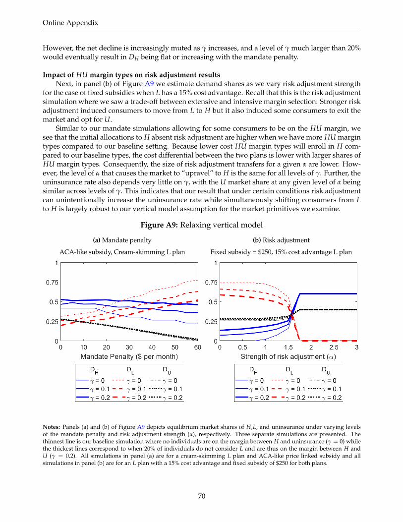
Online Appendix
However, the net decline is increasingly muted as γ increases, and a level of γ much larger than 20%would eventually result in DH being flat or increasing with the mandate penalty.
Impact of HU margin types on risk adjustment resultsNext, in panel (b) of Figure A9 we estimate demand shares as we vary risk adjustment strength
for the case of fixed subsidies when L has a 15% cost advantage. Recall that this is the risk adjustmentsimulation where we saw a trade-off between extensive and intensive margin selection: Stronger riskadjustment induced consumers to move from L to H but it also induced some consumers to exit themarket and opt for U.
Similar to our mandate simulations allowing for some consumers to be on the HU margin, wesee that the initial allocations to H absent risk adjustment are higher when we have more HU margintypes compared to our baseline setting. Because lower cost HU margin types will enroll in H com-pared to our baseline types, the cost differential between the two plans is lower with larger shares ofHU margin types. Consequently, the size of risk adjustment transfers for a given α are lower. How-ever, the level of α that causes the market to “upravel” to H is the same for all levels of γ. Further, theuninsurance rate also depends very little on γ, with the U market share at any given level of α beingsimilar across levels of γ. This indicates that our result that under certain conditions risk adjustmentcan unintentionally increase the uninsurance rate while simultaneously shifting consumers from Lto H is largely robust to our vertical model assumption for the market primitives we examine.
Figure A9: Relaxing vertical model
(a) Mandate penalty
ACA-like subsidy, Cream-skimming L plan
(b) Risk adjustment
Fixed subsidy = $250, 15% cost advantage L plan
Notes: Panels (a) and (b) of Figure A9 depicts equilibrium market shares of H,L, and uninsurance under varying levelsof the mandate penalty and risk adjustment strength (α), respectively. Three separate simulations are presented. Thethinnest line is our baseline simulation where no individuals are on the margin between H and uninsurance (γ = 0) whilethe thickest lines correspond to when 20% of individuals do not consider L and are thus on the margin between H andU (γ = 0.2). All simulations in panel (a) are for a cream-skimming L plan and ACA-like price linked subsidy and allsimulations in panel (b) are for an L plan with a 15% cost advantage and fixed subsidy of $250 for both plans.
70

Online Appendix
D.4.2 Empirical Robustness: Varying ∆WHL
Demand for H critically depends on the incremental willingness to pay for H relative to L, ∆WHL =WH(s)−WL(s). Below, we see how sensitive our results are to variations in this incremental willing-ness to pay. Specifically, we estimate equilibrium under simulations where we hold fixed WL(s) atbaseline but scale ∆WHL(s) by a multiplier ρ ∈ [0.25, 4]:
∆WadjHL(s) = ∆WHL(s)raw ∗ ρ
WadjH (s) = WL(s) + ∆Wadj
HL(s)
This scaling changes both the level and slope of WH(s), as seen in Figure A10.Using our typical counterfactual process, we estimate equilibrium market shares under these
modified primitives for varying levels of the mandate penalty and risk adjustment strength. Simula-tion results are presented in Figure A11. We find that under both increased and decreased incrementalwillingness to pay (i.e. higher and lower ρ), the general patterns of our counterfactual exercises donot change.
Panel (a) shows that demand for H declines with a larger mandate penalty, except at the veryhigh scalar ρ = 4. When ρ = 4, the marginal willingness to pay for H relative to L is sufficientlyhigh that an incrementally higher mandate penalty induces individuals to enter the market and thenchoose H over L. As a result, demand for H is weakly increasing in the mandate penalty throughoutthe range of penalties tested while demand for L only rises for high levels of the mandate. The risein L only occurs in the range of mandate penalties where the individuals induced to enter the marketare of sufficiently low marginal willingness to pay that some choose L instead of H. Because this is arelatively small group, the cost differential between H and L remains small.
Panel (b) shows that increasing the strength of risk adjustment has similar effects at all levels ofρ. Initially, stronger risk adjustment induces consumers to choose H instead of L. But in all cases,there is also eventually an unintended increase in the uninsurance rate. The effect of modifying ρ isthat the shifts in market share (both from L to H and from L to U) occur at different levels of α withshifts occurring at lower levels of α for higher levels of ρ. That is, when marginal willingness to payfor H relative to L is higher, a lower level of risk adjustment is needed to induce changes in marketshares.
71

Online Appendix
Figure A10: Scaled WTPH
(a) Low income demand
(b) High income demand
Notes: Panels (a) and (b) of A10 depicts willingness to pay curves for high and low-income consumers, respectively, undervarious scaling factors ρ of ∆Wadj
HL = ρ∆WHL. The thickest lines are for high marginal WTP for H relative to L. Baseline isfor ρ = 1. Willingness to pay for L is the dashed line and remains unmodified.
72

Online Appendix
Figure A11: Scaling ∆WTP
(a) Mandate penalty
ACA-like subsidy, Cream-skimming L plan
(b) Risk adjustment
Fixed subsidy = $250, 15 % cost advantage L plan
Notes: Figure A11 shows market shares for H,L, and uninsurance under the different scaled ∆WTP curves depicted infigure A10. Panel (a) depicts shares for different mandate penalties under an ACA-like price-linked subsidy and cream-skimming L plan (∆CHL = 0). Panel (b) depicts shares for different strengths of risk adjustment (α) under a fixed subsidyand a 15% L plan cost advantage. As in figure A10, thicker lines correspond to market shares when marginal willingnessto pay for H relative to L is set higher (higher ρ).
73