Bank of Canada staff working papers provide a forum for staff to publish work-in-progress research independently from the Bank’s Governing Council. This research may support or challenge prevailing policy orthodoxy. Therefore, the views expressed in this paper are solely those of the authors and may differ from official Bank of Canada views. No responsibility for them should be attributed to the Bank.

www.bank-banque-canada.ca

Staff Working Paper/Document de travail du personnel 2018-57

The Trade War in Numbers

by Karyne B. Charbonneau and Anthony Landry

ISSN 1701-9397 © 2018 Bank of Canada

Bank of Canada Staff Working Paper 2018-57

November 2018

The Trade War in Numbers

by

Karyne B. Charbonneau and Anthony Landry

Canadian Economic Analysis Department Bank of Canada

Ottawa, Ontario, Canada K1A 0G9 kcharbonneau@bankofcanada.ca anthonylandry@bankofcanada.ca

i

Acknowledgements

We thank Lorenzo Caliendo, Samuel Kortum, Sylvain Leduc, and Daniel Trefler for their insightful comments and suggestions. Jacob Dolinar and Pujan Thakrar provided excellent research assistance. The views expressed in this paper are our own and should not be interpreted as reflecting the views of the Bank of Canada. All remaining errors are our own.

ii

Abstract

We build upon new developments in the international trade literature to isolate and quantify the long-run economic impacts of tariff changes on the United States and the global economy. In particular, we apply the most recent data and trade elasticity estimates to the Ricardian model of Caliendo and Parro (2015) to quantify the long-run impacts of the recently applied and proposed tariff changes, including the U.S. tariffs on steel and aluminum imports and the rounds of additional tariffs between the United States and China. To fit the reality of the current trade policy shift, our analysis also allows for quotas and endogenizes trade balances. Overall, our results suggest that the newly imposed and proposed tariff schemes imply considerable changes in trade flows and sectoral output reallocations, but modest impacts on long-run aggregate prices and output levels. Bank topics: Recent economic and financial developments; Trade integration JEL codes: F11, F13, F14, F15, F50, F62, F68

Résumé

Nous nous appuyons sur les travaux récents de la littérature consacrée au commerce international pour isoler et quantifier les effets économiques à long terme des modifications des droits de douane sur les États-Unis et l’économie mondiale. Nous intégrons les données les plus récentes et nos estimations de l’élasticité des échanges commerciaux au modèle ricardien de Caliendo et Parro (2015), afin de calculer l’incidence économique à long terme des droits de douane récemment imposés et proposés, y compris les droits sur les importations d’acier et d’aluminium mis en place par l’administration américaine et les séries de droits de douane supplémentaires appliqués entre les États-Unis et la Chine. Pour rendre compte de l’orientation actuelle de la politique commerciale, notre cadre d’analyse inclut les quotas et endogénéise les balances commerciales. Dans l’ensemble, les résultats obtenus semblent indiquer que les nouveaux droits de douane imposés et proposés ont des répercussions considérables sur les flux commerciaux et la réallocation de la production entre les secteurs. Toutefois, nous estimons que les conséquences à long terme sont modestes sur le niveau général des prix et les niveaux de production. Sujets : Évolution économique et financière récente; Intégration des échanges Codes JEL : F11, F13, F14, F15, F50, F62, F68

Non-Technical Summary

Quantifying the impact of tariff changes has become a priority for many policy institutions, given the recent rising trade tensions. In this paper, we build upon new developments in the international trade literature to isolate and quantify the long-run economic impacts of tariff changes on the United States and the global economy. In particular, we apply the most recent data and trade elasticity estimates to the Ricardian model of Caliendo and Parro (2015) to quantify the long-run impacts of the recently applied and proposed tariff changes, including the U.S. tariffs on steel and aluminum imports, the rounds of additional tariffs between the United States and China, and potential U.S tariffs on the imports of automobiles and parts. To fit the reality of the current trade policy shift, our analysis also allows for quotas and endogenizes trade balances.

We use the Caliendo and Parro (2015) model in our benchmark analysis because of its many attractive features that allow us to precisely isolate and quantify the long-run impacts of tariff changes. First, it is a Ricardian model of trade (e.g., Eaton and Kortum (2002)). This implies that differences in technology, across sectors and countries, drive comparative advantage and trade. Second, the model has multiple countries and sectors, with interactions across tradable and non-tradable sectors observed in the input-output tables. Therefore, it allows for trade between countries that are different in terms of resources or technology, including different stages of development. In addition, the model explicitly incorporates trade in intermediate goods, which allows us to capture global value chains and to understand the impact of tariff changes on key systemic sectors of the economy. Third, the model's solution allows us to specifically isolate the long-run impacts of tariff changes from other economic developments. Finally, the multi-sector aspect of the model with input-output linkages allows us to run counterfactual scenarios on tariffs targeted to particular sectors or goods, and to understand how these targeted tariffs ripple through the economy.

We summarize the impact of the recently imposed and planned tariffs on the United States and the global economy by decomposing the events that have happened to date into two layers. First, we look into the recently applied U.S. tariffs on steel and aluminum imports and the following rounds of retaliation by U.S. trading partners. We then look at the impacts of potential U.S tariffs on the imports of automobiles and parts. Overall, our results suggest that the newly imposed and proposed tariff schemes imply considerable changes in trade flows and sectoral output reallocations, but modest impacts on long-run aggregate prices and output levels. The implied large sectoral output reallocations, however, suggest important short-run price movements, as they appear too large to be absorbed given the current industry structure, as many sectors of the U.S. and global economies already face capacity pressures.

1 IntroductionQuantifying the impact of tariff changes has become a priority for many policy institutions, given the recentrising trade tensions. In this paper, we build upon new developments in the international trade literature toisolate and quantify the long-run economic impacts of tariff changes on the United States and the globaleconomy. In particular, we apply the most recent data and trade elasticity estimates to the Ricardian modelof Caliendo and Parro (2015) to quantify the long-run impacts of the recently applied and proposed tariffchanges, including the U.S. tariffs on steel and aluminum imports, the rounds of additional tariffs betweenthe United States and China, and potential U.S tariffs on the imports of automobiles and parts. To fit thereality of the current trade policy shift, our analysis also allows for quotas and endogenizes trade balances.

We use the Caliendo and Parro (2015) model in our benchmark analysis because of its many attractivefeatures that allow us to precisely isolate and quantify the long-run impacts of tariff changes. First, it is a Ri-cardian model of trade (e.g., Eaton and Kortum (2002)). This implies that differences in technology, acrosssectors and countries, drive comparative advantage and trade.1 Second, the model has multiple countriesand sectors, with interactions across tradable and non-tradable sectors observed in the input-output tables.Therefore, it allows for trade between countries that are different in terms of resources or technology, in-cluding different stages of development. In addition, the model explicitly incorporates trade in intermediategoods, which allows us to capture global value chains and to understand the impact of tariff changes on keysystemic sectors of the economy. Third, the model’s solution allows us to specifically isolate the long-runimpacts of tariff changes from other economic developments. Finally, the multi-sector aspect of the modelwith input-output linkages allows us to run counterfactual scenarios on tariffs targeted to particular sectorsor goods, and to understand how these targeted tariffs ripple through the economy.

We summarize the impact of the recently imposed and planned tariffs on the United States and the globaleconomy by decomposing the events that have happened to date into two layers. First, we look into the re-cently applied U.S. tariffs on steel and aluminum imports and the following rounds of retaliation by U.S.trading partners. Our main finding is that Canada, Mexico, and the United States see the largest impacts ontheir trade flows and real GDP. For example, U.S. real GDP falls by 0.05 percent, while U.S. exports fall by2.2 percent. In particular, we find that U.S. exports fall in many sectors, reflecting the importance of steeland aluminum as an input in U.S. exports. As such, U.S. exports fall not only because of other countries’retaliatory tariffs on American products, but also because the cost for U.S. firms producing goods for ex-ports rises and makes them less competitive in the global market. Globally, the U.S. tariffs and the followingrounds of retaliations represent a world output loss of 0.02 percent or $13.7 billion (in 2018 dollars at marketexchange rates) using International Monetary Fund (2018) world output estimates.

We also found that the U.S. administration appeared too optimistic regarding its assessments of the steeland aluminum imports drop and production increase from the newly imposed tariffs. Abstracting from re-taliations, the model simulation implies a 34 percent drop in U.S. intermediate metals imports (the sectorthat includes most steel and aluminum products). This suggests an intermediate metals imports drop almosttwice as big as the target identified in Department of Commerce documents (U.S. Department of Commerce(2018a), U.S. Department of Commerce (2018b)). The model simulation also suggests an intermediate met-als real GDP increase of only 4.5 percent (7.9 percent without retaliations). This also appears to be far belowthe implied increase of 10 percent in intermediate metals production targeted by the U.S. administration.

1Comparative advantage is a country’s ability to produce a good at a lower cost relative to other goods and othercountries, based on technology, and taking into account geography, tariffs, quotas, and other trade barriers.

2

Next, we consider the impacts of the rising tension in the U.S.-China trade relationship. Here, we addthe two rounds of U.S. tariffs on Chinese imports with China’s retaliations, in addition to the steel and alu-minum tariffs discussed above. The model suggests that the proposed January 2019 tariff scheme impliesa U.S. real GDP decline of 0.25 percent and a U.S. exports decline of 10.4 percent—with a broad-baseddecline in exports to China of 52.7 percent. In particular, the newly imposed and proposed tariffs imply im-portant sectoral price adjustments, as well as sectoral export and output reallocations. Globally, the modelsuggests that the proposed tariff scheme represents a world output loss of 0.1 percent or $81.4 billion (in2018 dollars at market exchange rates)—which roughly represents the size of the economy of the DominicanRepublic. The impacts on global trade, however, are much more pronounced, with a global exports declineof 1.4 percent or $250 billion (in 2018 dollars at market exchange rates)—slightly bigger than the economyof Portugal or Greece.

Our model suggests that U.S.-China trade tensions ripple through the global economy, especially amongCanada, Mexico, and other Asian economies that either are part of the global supply chain affected by thetariffs or that offer close substitutes to Chinese and U.S. exports. In particular, Canada and Mexico seesizable output reallocation toward many tradable sectors that provide the U.S. with a close substitute tomajor Chinese export sectors (e.g., clothing, medical and communication, electrical machinery, machinery,and other manufacturing). These sizable and broad-based sectoral output reallocations for the U.S. and itstrading partners suggest important short-run price movements, as they appear too large to be absorbed bythe current industry structure given the slow movements of labor and capital across sectors. In fact, some ofthe sectors with the largest growth rates already face substantial capacity pressure.2

As in Caliendo and Parro (2015), the results above assume that trade balances remain fixed following achange in tariff schemes. In the current context, however, this assumption may be misleading as trade rebal-ancing is at the forefront of the current U.S.-led trade war. As expected, the additional U.S. tariffs reduce theU.S. trade deficit and the Chinese surplus, but the main takeaway is that endogenizing trade balances doesnot change the qualitative results. As pointed out, the United States depends on imported inputs for manysectors of its economy. As such, U.S. exports fall not only because of other countries’ retaliatory tariffson U.S. exports, but also because the cost for U.S. firms producing goods for exports rises and makes U.S.exports less competitive on the global market. The end results are lower imports, lower exports, and littleimprovement in the U.S. trade deficit.

This paper is closely related to the trade literature that quantifies the impact of trade integration. Forexample, the original contribution of Caliendo and Parro (2015) was to estimate the effects of the NorthAmerican Free Trade Agreement (NAFTA) on consumer welfare and trade. Other notable quantitative stud-ies include Trefler (2004), who studies the impact of the Canada-U.S. free trade agreement on employmentand manufacturing plant productivity, Romalis (2007), who identifies NAFTA’s effects on trade volumesand prices, and more recently, Auer et al. (2018), who look at the income implications of revoking NAFTA.In contrast, Autor et al. (2013) analyze the effect of rising Chinese import competition on U.S. local labormarkets, while Amiti et al. (2017) analyze the effects of China’s rapid export expansion on U.S. prices.3 Inthis paper, we look at the price, trade, and output implications of the current shift in global tariff schemesinitiated by the United States in 2018.

2For example, Canadian and U.S. capacity utilization rates in many manufacturing sectors are currently close tohistorical highs.

3See Costinot and Rodrıguez-Clare (2014) and Maggi (2014) for an excellent review of recent theoretical andquantitative works on trade integration.

3

Our analysis also offers several advantages over many policy models that have been used to estimatethe impact of the current trade policy shift, such as the Global Trade Analysis Project (GTAP) (Corong etal. (2017)) or the Global Integrated Monetary and Fiscal Model (GIMF) (Anderson et al. (2013) and Inter-national Monetary Fund (2018)). For example, these models use Armington aggregates to bundle imports,while we allow consumers and producers to search for the lowest-cost supplier. In addition, our model ishighly disaggregated and uses input-output linkages, allowing us to run counterfactual scenarios on tariffstargeted to particular sectors or countries, and to understand how these targeted tariffs ripple to other sectoraland aggregate variables such as prices, trade flows, and production.

Overall, our results suggest that the newly imposed and proposed tariff schemes imply considerablechanges in trade flows and sectoral output reallocations, but modest impacts on long-run aggregate pricesand output levels. The implied large sectoral output reallocations, however, suggest important short-runprice movements, as they appear too large to be absorbed given the current industry structure, as manysectors of the U.S. and global economies already face capacity pressures. The rest of the paper proceedsas follows. In section 2, we present the main equations of the Caliendo and Parro (2015) model, which weuse as the backbone to run our tariff change scenarios. In section 3, we describe the data, show our recentsectoral trade elasticity estimates, and explain how we incorporate the newly imposed and proposed tariffsand quotas. In section 4, we present the estimated impacts of recently imposed and proposed tariffs on theUnited States and the global economy. In addition to the scenarios discussed above, section 4 also looks atthe impact of potential U.S tariffs on the imports of automobiles and parts. Finally, section 5 concludes.

2 The Economic EnvironmentOur economic environment builds on the Eaton and Kortum (2002) Ricardian model of trade and is similarto Caliendo and Parro (2015). The model features multiple regions, sectoral linkages and heterogeneityin production structures. Households receive income from labor income and tariff revenues. Labor is theonly factor of production, which is perfectly mobile across sectors but not across countries. The productiontechnology displays constant returns to scale, and all markets are perfectly competitive. Finally, internationaltrade in goods is costly because of transportation costs and tariffs. Below, we present the main equations ofthe Caliendo and Parro (2015) model, which we use as the backbone to run our tariff change scenarios, anddiscuss its equilibrium equations.4

The Caliendo-Parro model

Households

In each country, representative households maximize utility by consuming a plethora of final goods Cjnaccording to Cobb-Douglas preferences:

u(Cn) =

J∏j=1

Cjnαjn , where

J∑j=1

αjn = 1. (1)

Households receive income In from tariff revenues and labor income wnLn, where wn represents countryn’s wage and Ln represents country n’s labor supply.

4A more detailed version of the model and its solution are available in Caliendo and Parro (2015).

4

Intermediate goods

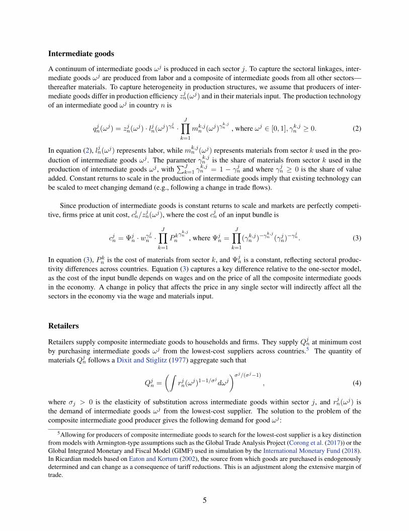
A continuum of intermediate goods ωj is produced in each sector j. To capture the sectoral linkages, inter-mediate goods ωj are produced from labor and a composite of intermediate goods from all other sectors—thereafter materials. To capture heterogeneity in production structures, we assume that producers of inter-mediate goods differ in production efficiency zjn(ωj) and in their materials input. The production technologyof an intermediate good ωj in country n is

qjn(ωj) = zjn(ωj) · ljn(ωj)γjn ·

J∏k=1

mk,jn (ωj)γ

k,jn , where ωj ∈ [0, 1], γk,jn ≥ 0. (2)

In equation (2), ljn(ωj) represents labor, while mk,jn (ωj) represents materials from sector k used in the pro-

duction of intermediate goods ωj . The parameter γk,jn is the share of materials from sector k used in theproduction of intermediate goods ωj , with

∑Jk=1 γ

k,jn = 1 − γjn and where γjn ≥ 0 is the share of value

added. Constant returns to scale in the production of intermediate goods imply that existing technology canbe scaled to meet changing demand (e.g., following a change in trade flows).

Since production of intermediate goods is constant returns to scale and markets are perfectly competi-tive, firms price at unit cost, cjn/z

jn(ωj), where the cost cjn of an input bundle is

cjn = Ψjn · wγ

jnn ·

J∏k=1

P knγk,jn , where Ψj

n =J∏k=1

(γk,jn )−γk,jn (γjn)−γ

jn . (3)

In equation (3), P kn is the cost of materials from sector k, and Ψjn is a constant, reflecting sectoral produc-

tivity differences across countries. Equation (3) captures a key difference relative to the one-sector model,as the cost of the input bundle depends on wages and on the price of all the composite intermediate goodsin the economy. A change in policy that affects the price in any single sector will indirectly affect all thesectors in the economy via the wage and materials input.

Retailers

Retailers supply composite intermediate goods to households and firms. They supply Qjn at minimum costby purchasing intermediate goods ωj from the lowest-cost suppliers across countries.5 The quantity ofmaterials Qjn follows a Dixit and Stiglitz (1977) aggregate such that

Qjn =

(∫rjn(ωj)1−1/σ

jdωj)σj/(σj−1)

, (4)

where σj > 0 is the elasticity of substitution across intermediate goods within sector j, and rjn(ωj) isthe demand of intermediate goods ωj from the lowest-cost supplier. The solution to the problem of thecomposite intermediate good producer gives the following demand for good ωj :

5Allowing for producers of composite intermediate goods to search for the lowest-cost supplier is a key distinctionfrom models with Armington-type assumptions such as the Global Trade Analysis Project (Corong et al. (2017)) or theGlobal Integrated Monetary and Fiscal Model (GIMF) used in simulation by the International Monetary Fund (2018).In Ricardian models based on Eaton and Kortum (2002), the source from which goods are purchased is endogenouslydetermined and can change as a consequence of tariff reductions. This is an adjustment along the extensive margin oftrade.

5

rjn(ωj) =

(pjn(ωj)

P jn

)−σj

Qjn, (5)

where P jn is the unit price of materials such that

P jn =

(∫pjn(ωj)1−σ

jdωj)1/(1−σj)

, (6)

and where pjn(ωj) denotes the lowest price of intermediate good ωj across all locations n where it can bedelivered. In turn, composite intermediate goods from sector j are used as materials for the production ofintermediate good ωk in the amount mj,k

n (ωk) in all sectors k, and as final goods in consumption Cjn. Assuch, the market clearing condition for the intermediate and final goods sector j is

Qjn = Cjn +J∑k=1

∫mj,kn (ωk)dωk. (7)

Trade costs and prices

We consider two types of trade costs. First, a transportation cost or iceberg cost is defined in physical unitsas in Samuelson (1954), where one unit of a tradable intermediate good in sector j shipped from country ito country n requires producing djni ≥ 1 units in i, with djnn = 1. Second, an ad-valorem flat-rate tariff τ jniapplicable over unit prices. Combining both trade costs leads to the following:

κjni = (1 + τ jni) · djni. (8)

After taking into account trade costs, a unit of a tradable intermediate good ωk produced in country i isavailable in country n at unit prices cjiκ

jni/z

ji (ω

j). Therefore, the price of intermediate good ωk in countryn is given by

pjn(ωj) = mini

(cjiκ

jni

zji (ωj)

). (9)

The tradable and the non-tradable sectors are identical, except that κjni = ∞ in the non-tradable sector.Thus, it is always cheaper to buy goods from local suppliers in the non-tradable sector.

Ricardian motives to trade are introduced following the Eaton and Kortum (2002) probabilistic repre-sentation of technologies allowing productivities to differ by country and sector. As such, we assume thatthe efficiency of producing a good ωj in country n is the realization of a Frechet distribution with a locationparameter that varies by country and sector λjn ≥ 0 and shape parameter that varies by sector θj . In thecontext of this model, a higher λjn ≥ 0 implies higher average sectoral productivity—a notion of absoluteadvantage—whereas a smaller value of θj implies higher dispersion of productivity across goods ωj—anotion of comparative advantage. We assume that the distributions of productivities are independent acrossgoods, sectors, and countries, and that 1 + θj > σj . With these assumptions, the price of the compositeintermediate good is given by

P jn = Aj

(N∑i=1

λji (cjiκjni)−θj)−1/θj

, (10)

6

for all sectors j and countries n.

Finally, with Cobb-Douglas preferences, the consumption price index is given by

Pn =J∏j=1

(P jn

αjn

)αjn

. (11)

Expenditure shares

Total expenditure on sector j goods in country n is given by

Xjn = P jnQ

jn. (12)

Denote Xjni to be the expenditure in country n of sector j goods from country i. It follows that country n’s

share of expenditure on goods j from i is given by

πjni =Xjni

Xjn

, (13)

which is also the probability that country i provides goods at the lowest cost to country n. Using theproperties of the Frechet distribution, we can derive expenditure shares as a function of technologies, pricesand trade costs:

πjni =λji (c

jiκjni)−θj∑N

h=1 λjh(cjhκ

jnh)−θj

. (14)

Notice that changes in tariffs have a direct effect on trade shares via the trade cost κjni, and an indirecteffect through the input bundles cost cjn—since it incorporates all the information contained in input-outputlinkages.

Total expenditure and trade balance

Total expenditure on sector j is the sum of the expenditure on composite intermediate goods by firms andexpenditure by households. Then, Xj

n is given by

Xjn =

J∑k=1

γjkn ·N∑i=1

πkin1 + τkin

Xki + αjnIn, (15)

where

In = wnLn +Rn +Dn. (16)

In this equation, In represents final absorption as the sum of labor income wnLn, tariff revenues Rn, andthe trade deficit Dn. Specifically,

Rn =

J∑j=1

N∑i=1

τ jniMjni, where M j

ni = Xjn

πjni1 + τ jni

represents imports, (17)

and

7

Dn =

J∑k=1

Dkn, and Dj

n =N∑i=1

M jni −

N∑i=1

Ejni, whereEjni = Xji

πjin1 + τ jin

represents exports. (18)

Aggregate trade deficits in each country are exogenous in the model, while sectoral trade deficits are en-dogenously determined.6

Finally, using the definition of expenditure and trade deficit we have that

J∑j=1

N∑i=1

πjni1 + τ jni

Xjn −Dn =

J∑j=1

N∑i=1

πjin1 + τ jin

Xji . (19)

This condition reflects the fact that total expenditure, excluding tariff payments, in country n minus tradedeficits equals the sum of each country’s total expenditure, excluding tariff payments, on tradable goodsfrom country n. In this environment, the equilibrium of the model can be described as follows:

Model’s equilibrium: Given Ln, Dn, λjn and djni, an equilibrium under policy τ is a wage vector w ∈ RN++

and prices {P jn}J,Nj=1,n=1 that satisfy equilibrium condition (3), (10), (14), (15), and (19) for all j, n.

Equilibrium in relative changesAs in Caliendo and Parro (2015), we solve for changes in prices and wages after changing from tariff sched-ules τ to τ ′, instead of solving for an equilibrium under tariff schedule τ . First, this allows us to conditionthe model on the state of the world in a base year. Second, this allows us to identify the effect on equilibriumoutcomes from a pure change in tariff schedules—which is what we are after in this paper. Finally, we cansolve for the general equilibrium of the model without needing to estimate parameters that are difficult toidentify in the data, as productivity parameters and iceberg cost vanish in differences. The equilibrium ofthe model in relative changes, that is, under tariff schedule τ ′ relative to a tariff schedule τ , can be describedas follows:

Equilibrium in relative changes: Let (w,P ) be an equilibrium under policy τ and let (w′, P ′) be an equi-librium under tariff schedule τ ′. Define (w, P ) as an equilibrium under τ ′ relative to τ , where a variablewith a hat “x” represents the relative change of the variable, namely x = x′/x. Using equations (3), (10),(14), (15), and (19), the equilibrium conditions in relative changes satisfy the following conditions:

1. Cost of the input bundles:

cjn = wγjnn ·

J∏k=1

P knγk,jn . (20)

2. Price index:

P jn =

(N∑i=1

πjni(cji κjni)−θj)−1/θj

. (21)

6The quantitative results are robust to whether we exogenously impose current aggregate trade surplus/deficits oraggregate balanced trade for each region.

8

3. Bilateral trade shares:

πjni =

(cji κ

jni

P jn

)−θj. (22)

4. Total expenditure in each country n and sector j:

Xjn′ =

J∑k=1

γjkn ·N∑i=1

πkin′

1 + τkin′Xki′ + αjnI

′n. (23)

5. Trade balance:J∑j=1

N∑i=1

πjni′

1 + τ jni′Xjn′ −Dn =

J∑j=1

N∑i=1

πjin′

1 + τ jin′Xji′, (24)

where

κjni =1 + τ jni

′

1 + τ jni, and I ′n = w′nLn +

J∑j=1

N∑i=1

τ jni′ πjni

′

1 + τ jni′Xjn′ +Dn. (25)

From inspecting equilibrium conditions 20-23, we can observe that the focus on relative changes allowsus to perform policy experiments without relying on estimates of total factor productivity or transport costs.We need only two sets of tariff structures (τ and τ ′), data on bilateral trade shares (πjni), the share of valueadded in production (γjn), value added (wnLn), the share of intermediate consumption (γk,jn ), and sectoraldispersion of productivity (θj). The share of each sector in final demand (αjn) is obtained from these data.In the next section, we briefly describe the data and the estimation of sectoral productivity dispersion (θj)—which is the only set of parameters to estimate.

3 Data and Estimation

3.1 Matching the model with the dataOur quantitative analysis includes 44 sectors and 16 regions. The sectors are divided into 24 tradable and 20non-tradable sectors, which are enumerated in Appendix A. We group sectors by commodities defined usingthe Harmonized Commodity Description and Coding System (HS) 2012 at the six-digit level of aggregationand concorded to two digits ISIC Revision 3. The regions include Australia, Brazil, Canada, China, theEuropean Union, India, Japan, Malaysia, Mexico, Norway, Peru, South Korea, Switzerland, Thailand, theUnited States, and a catch-all region named rest of world.

We use the most recent available data to get an up-to-date picture of the global economy. Data on bilat-eral trade flows are from the United Nations Statistical Division (UNSD) Commodity Trade (COMTRADE)database. We use an average of 2014 and 2015 bilateral trade flow data because some sectoral trade flowsare lumpy even at annual frequency (e.g., aircraft).7 Data on sectoral value added, gross production andinput-output tables are from the 2011 OECD Input-Output Database.8 We obtain measures of bilateral trade

7We choose to not incorporate the 2016 bilateral trade flow data because the recent oil price shock affected tradeflows significantly in 2016.

8At the time of publication, the 2011 OECD Input-Output Database was the most up-to-date database that ensuredconsistency across countries.

9

shares πjni, share of value added γjn, share of intermediate inputs γj,kn and share of final demand αjn usingdata on bilateral trade flows, value added, gross production, and input-output tables.

Finally, bilateral tariff data are from the WTO Tariff Database for the year 2016 at the HS 2012 six-digit level. They are aggregated into our 24 tradable sectors using the average of 2014 and 2015 bilateraltrade flow data. We use trade agreement tariffs (e.g., NAFTA) when lower than most-favored-nation (MFN)tariffs, and apply symmetric tariff schedules in cases where a trade agreement between two countries wasnot available for one of the countries in the WTO Tariff Database. Appendix B offers a detailed descriptionof the data.

3.2 Trade elasticity estimatesThe remaining parameters to measure are the trade elasticities. In the model, trade elasticities govern theextent of comparative advantage and are key parameters for our quantitative scenario analysis. For example,a low trade elasticity implies a high productivity dispersion across countries. This means that a retailer’scurrent supplier is likely to remain its lowest-cost supplier when trade costs increase. As such, an increasein tariffs or other trade costs has a small impact on trade flows.

We estimate trade elasticities using tariff schedules and bilateral trade flow data following Caliendo andParro (2015). Specifically, our estimating equation is

ln

(XjniX

jihX

jhn

XjinX

jhiX

jnh

)= −θj ln

(τ jniτ

jihτ

jhn

τ jinτjhiτ

jnh

)+ εj , (26)

where τni = (1 + τni) for all n, h, i.

Our trade elasticity estimates and their standard errors are presented in Table 1. The elasticity estimatesrange from a high degree of substitutability of 69.1 in the other energy sector (e.g., coal) to a low of 1.1 inthe farm sector. For example, the intermediate metals sector (e.g., steel and aluminum) elasticity estimateis in the mid-range of 6.2. From (22), this implies that a 10 percent increase in tariffs reduces the sectoralimport shares by 45 percent—keeping everything else constant. These estimates are in the range of the tradeelasticity estimates in the literature.9

The dispersion in trade elasticity shown in Table 1 highlights differences in sectoral sensitivity to tariffchanges. The equality of parameter estimates across sectors is strongly rejected by an F-test. Although thefocus of this paper is on sectoral trade elasticities and input-output linkages, we nevertheless estimate anaggregate trade elasticity by running (26) on all sectoral data. For example, this is the trade elasticity thatwould be used in a one-sector model such as Eaton and Kortum (2002). On aggregate, our trade elasticityestimate is 2.7, which is in the range of the estimates in the literature. Notice, however, that this aggregateelasticity estimate is much lower than the sectoral average of 12.0. See Imbs and Mejean (2015) and Si-monovska and Waugh (2014) for a discussion on this issue and other recent advances.

Table 1 also shows the trade elasticities reported in Caliendo and Parro (2015). These are based on 1993data, the year before NAFTA came into force. Elasticities computed using 1996 tariffs and trade data showthat the difference between our estimates and those of Caliendo and Parro (2015) are due to a change in

9These estimates are robust to the removal of different types of outliers. In the esimates presented in Table 1, wetake out countries that have less than 0.1 percent of world trade. We also remove Switzerland.

10

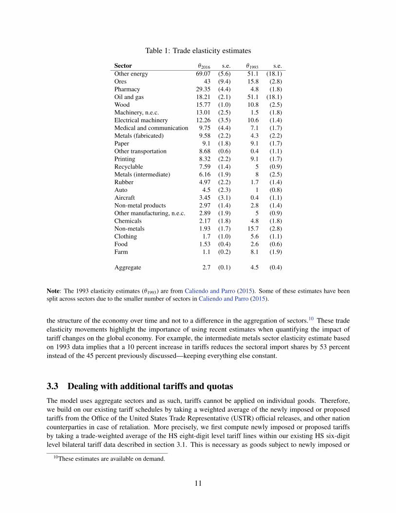
Table 1: Trade elasticity estimates

Sector θ2016 s.e. θ1993 s.e.Other energy 69.07 (5.6) 51.1 (18.1)Ores 43 (9.4) 15.8 (2.8)Pharmacy 29.35 (4.4) 4.8 (1.8)Oil and gas 18.21 (2.1) 51.1 (18.1)Wood 15.77 (1.0) 10.8 (2.5)Machinery, n.e.c. 13.01 (2.5) 1.5 (1.8)Electrical machinery 12.26 (3.5) 10.6 (1.4)Medical and communication 9.75 (4.4) 7.1 (1.7)Metals (fabricated) 9.58 (2.2) 4.3 (2.2)Paper 9.1 (1.8) 9.1 (1.7)Other transportation 8.68 (0.6) 0.4 (1.1)Printing 8.32 (2.2) 9.1 (1.7)Recyclable 7.59 (1.4) 5 (0.9)Metals (intermediate) 6.16 (1.9) 8 (2.5)Rubber 4.97 (2.2) 1.7 (1.4)Auto 4.5 (2.3) 1 (0.8)Aircraft 3.45 (3.1) 0.4 (1.1)Non-metal products 2.97 (1.4) 2.8 (1.4)Other manufacturing, n.e.c. 2.89 (1.9) 5 (0.9)Chemicals 2.17 (1.8) 4.8 (1.8)Non-metals 1.93 (1.7) 15.7 (2.8)Clothing 1.7 (1.0) 5.6 (1.1)Food 1.53 (0.4) 2.6 (0.6)Farm 1.1 (0.2) 8.1 (1.9)

Aggregate 2.7 (0.1) 4.5 (0.4)

Note: The 1993 elasticity estimates (θ1993) are from Caliendo and Parro (2015). Some of these estimates have beensplit across sectors due to the smaller number of sectors in Caliendo and Parro (2015).

the structure of the economy over time and not to a difference in the aggregation of sectors.10 These tradeelasticity movements highlight the importance of using recent estimates when quantifying the impact oftariff changes on the global economy. For example, the intermediate metals sector elasticity estimate basedon 1993 data implies that a 10 percent increase in tariffs reduces the sectoral import shares by 53 percentinstead of the 45 percent previously discussed—keeping everything else constant.

3.3 Dealing with additional tariffs and quotasThe model uses aggregate sectors and as such, tariffs cannot be applied on individual goods. Therefore,we build on our existing tariff schedules by taking a weighted average of the newly imposed or proposedtariffs from the Office of the United States Trade Representative (USTR) official releases, and other nationcounterparties in case of retaliation. More precisely, we first compute newly imposed or proposed tariffsby taking a trade-weighted average of the HS eight-digit level tariff lines within our existing HS six-digitlevel bilateral tariff data described in section 3.1. This is necessary as goods subject to newly imposed or

10These estimates are available on demand.

11

proposed tariffs are often described at the HS eight-digit level.11 Then, we update our tariff schedules byadding these additional tariffs to our existing tariff schedule. A broader description of the tariff data and adetailed timeline of additional tariff events are available in Appendix C.

Some of the new trade barriers also involve quotas. For example, the U.S. imposed absolute quotas onsteel from Brazil and South Korea. To reflect such measures in our counterfactual analysis, we impose aquota on an entire sector when the majority of that sector is affected by the quota. For example, 65 percentof Brazilian nominal exports of intermediate metals is affected by the steel quotas, while this number is 77percent for South Korea. Therefore, we impose a quota on U.S. imports of intermediate metals from Braziland South Korea. In contrast, washing machines and solar panels, for which quotas were also imposed,represent only an average of 9 percent of the electrical machinery sector.12 Since they represent such a smallfraction, these quotas are not taken into account in our counterfactual analysis. We choose to impose quotasrather than tariff equivalents in order to maintain an accurate redistribution of wealth (i.e., no collection oftariffs by the U.S.). As mentioned above, quotas are applied on the entirety of a sector as a percentage ofour nominal baseline trade data affected by the quota. This has the caveat of not allowing other parts ofthe sector to respond to changes in the economic environment. We further assume the quotas to always bebinding.13

Note that throughout the paper, the baseline is the 2016 tariff schedule, and therefore abstracts fromtrade actions taken between 2016 and early 2018. More specifically, our baseline abstracts from two setsof tariffs imposed prior to the steel and aluminum tariffs. The first concerns the softwood lumber disputebetween Canada and the U.S. The tariffs imposed in this context are anti-dumping and countervailing dutiesand are temporary in nature. We therefore do not include them. The second are the early 2018 tariffs andquotas on solar panels and washing machines. As explained above, we do not include these measures dueto their large quota component on a small fraction of goods in the electrical machinery sector.

4 The Trade War in NumbersIn this section, we present the estimated impacts of recently imposed and proposed tariffs on the UnitedStates and the global economy. In particular, we present the impact on prices, trade flows, and real GDP.Since this is a one-factor model, the latter correspond to the real wage impacts.14 Below, we first estimate

11HS codes are not harmonized across countries at a more detailed level than six digits. Therefore, we can only getthis level of detail in our analysis for U.S. imposed tariffs. For all other countries, we impose the tariff on the six-digitgood associated with the eight-digit good(s) targeted. A caveat of this limitation is that it may lead to an overstatementof the trade amount affected by the tariffs. In fact, the U.S. data suggest that there could be a sizable difference.However, the trade values affected by tariffs found using this method are in line with the numbers announced by therespective governments.

12The only country where it represents a significant share is Malaysia, with 49 percent of electrical machineryexports to the U.S.

13This assumption is supported by the model: given the steel and aluminum tariffs, if no tariffs were appliedto imports of intermediate metals from Brazil and South Korea, the model would suggest a large increase in thoseimports.

14We do not report welfare effects as in Caliendo and Parro (2015) as we want to abstract from questions or redis-tribution of tariff revenues. In that sense our estimates compare to studies that evaluate the effects of trade opennesswhen there are no tariffs, such as Arkolakis et al. (2012).

12

the impacts of the trade war saga to date. Then, we look at the implications of endogenizing trade balances.Finally, we consider the effects of potential tariffs on automobiles and automobile parts.15

4.1 The trade war sagaWe summarize the impact of the recently imposed and planned tariffs on the United States and the globaleconomy by decomposing the events that have happened so far in two parts: the recently applied U.S. tariffson steel and aluminum imports and the following rounds of retaliation by U.S. trading partners, and therecently applied and proposed U.S. tariffs on Chinese goods imports and the following rounds of Chineseretaliation. We dig into the steel and aluminum tariffs saga first because it allows us to more easily developa story and to gain economic intuitions, as the U.S. import tariffs are mostly concentrated in one tradablesector of the economy: intermediate metals. Our baseline for this exercise is the 2016 global tariff scheduledescribed in the previous section.

Part 1: Steel and aluminum tariffs

On March 1, 2018, President Trump announced his intention to impose a 25 percent tariff on steel and a10 percent tariff on aluminum imports.16 A number of countries have retaliated following the impositionof U.S. tariffs on steel and aluminum imports. In particular, Canada, China, and the European Union im-posed retaliatory tariffs on a number of products, ranging from U.S. steel and aluminum products to iconicAmerican products such as Jack Daniel’s and Harley-Davidson motorcycles. The distribution of U.S. andretaliatory tariffs across sectors are displayed in Figure 1. The U.S. tariffs on steel and aluminum importsare concentrated in the intermediate metals sector, while the retaliatory tariffs on U.S. exports are morebroadly distributed across sectors.

First, we consider the macroeconomic impacts of the steel and aluminum tariffs on the United Statesand its trading partners, without retaliations. This will allow us to get a clear picture of the mechanismsunderlying the impacts of U.S. tariffs on steel and aluminum on the global economy. Then, we look at theimpacts of the steel and aluminum tariffs with trading partner retaliation. Finally, we look into sectoralexports, prices, and output reallocation implications of these additional tariffs for the global economy.

Panel A of Table 2 displays the global impacts from the U.S. tariffs on steel and aluminum imports ontrade flows, terms of trade, GDP deflators, and real GDP across countries without retaliation. Overall, themain takeaway is that the countries that see the largest impacts on their trade flows, terms of trade, and realGDP are Canada, Mexico, and the United States. For example, Canada experiences the largest decrease inexports among U.S. trading partners because it has the largest share of exports exposed to the U.S. steel and

15The results presented below are qualitatively robust to the trade elasticity estimates.16U.S. steel and aluminum tariffs are applied to all countries except Australia. Absolute quotas on steel from Brazil

and South Korea are set to 70 percent of the average steel volume of exports to the United States (100 percent for Brazilsemi-finished steel products) from these countries between 2015 and 2017. Here, we treat U.S. steel and aluminumquotas as binding for Brazil and South Korea and set an effective quota on intermediate metals sector exports of bothcountries to the U.S. These quotas are set at 94 percent and 77 percent of the baseline nominal trade data, for Braziland South Korea respectively, to reflect the share of steel in each country’s exports of intermediate metals. If Braziland South Korea had chosen to have their steel exports submitted to the tariffs rather than take a quota restriction, theirexports would have fallen much more. The model suggests that they are better off with the quota. We do not includethe U.S. steel and aluminum tariffs exemption of Argentina and the Turkish retaliation because they are part of the restof the world region.

13

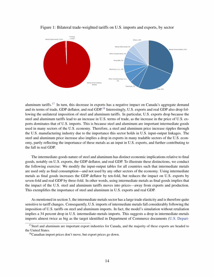
Figure 1: Bilateral trade-weighted tariffs on U.S. imports and exports, by sector

Metals (intermediate), 98.94%

Metals (fabricated), 0.53%

Printing,0.53%

Metals (intermediate), 31%

Food, 25%

Chemicals, 7%

Other manufacturing, n.e.c., 6%

Machinery, n.e.c., 6%

Recyclable, 5%

Other transportation, 5%

Metals (fabricated), 5%

Others, 10%

aluminum tariffs.17 In turn, this decrease in exports has a negative impact on Canada’s aggregate demandand its terms of trade, GDP deflator, and real GDP.18 Interestingly, U.S. exports and real GDP also drop fol-lowing the unilateral imposition of steel and aluminum tariffs. In particular, U.S. exports drop because thesteel and aluminum tariffs lead to an increase in U.S. terms of trade, as the increase in the price of U.S. ex-ports dominates that of U.S. imports. This is because steel and aluminum are important intermediate goodsused in many sectors of the U.S. economy. Therefore, a steel and aluminum price increase ripples throughthe U.S. manufacturing industry due to the importance this sector holds in U.S. input-output linkages. Thesteel and aluminum price increase also implies a drop in exports in many tradable sectors of the U.S. econ-omy, partly reflecting the importance of these metals as an input in U.S. exports, and further contributing tothe fall in real GDP.

The intermediate-goods nature of steel and aluminum has distinct economic implications relative to finalgoods, notably on U.S. exports, the GDP deflator, and real GDP. To illustrate these distinctions, we conductthe following exercise: We modify the input-output tables for all countries such that intermediate metalsare used only as final consumption—and not used by any other sectors of the economy. Using intermediatemetals as final goods increases the GDP deflator by ten-fold, but reduces the impact on U.S. exports byseven-fold and real GDP by three-fold. In other words, using intermediate metals as final goods implies thatthe impact of the U.S. steel and aluminum tariffs moves into prices—away from exports and production.This exemplifies the importance of steel and aluminum in U.S. exports and real GDP.

As mentioned in section 3, the intermediate metals sector has a large trade elasticity and is therefore quitesensitive to tariff changes. Consequently, U.S. imports of intermediate metals fall considerably following theimposition of U.S. tariffs on steel and aluminum imports. In fact, the model’s simulation without retaliationimplies a 34 percent drop in U.S. intermediate-metals imports. This suggests a drop in intermediate-metalsimports almost twice as big as the target identified in Department of Commerce documents (U.S. Depart-

17Steel and aluminum are important export industries for Canada, and the majority of these exports are headed tothe United States.

18Canadian import prices don’t move, but export prices go down.

14

Table 2: Global impacts from U.S. tariffs on steel and aluminum(in percent change)

Panel A: No retaliationExposure Change in Trade Flows Terms of GDP Real

Tariffs X to U.S. X to U.S. Total X Total M Trade Deflator GDPAustralia 0.12 4.34 2.52 -0.05 -0.05 0.00 0.01 0.00Brazil 1.38 12.44 -0.48 -0.11 -0.12 0.00 0.01 0.00Canada 2.81 76.09 -1.50 -0.81 -0.80 -0.05 -0.08 -0.05China 0.19 17.53 -0.16 0.02 0.03 0.00 0.02 0.00EU 0.17 7.38 -1.53 -0.02 -0.02 0.00 0.00 0.00India 0.40 14.30 -1.88 -0.19 -0.14 0.00 -0.01 -0.01Japan 0.42 19.65 -1.05 -0.08 -0.08 0.00 0.01 0.00Korea 0.73 12.80 -1.13 -0.06 -0.08 0.00 0.01 0.00Malaysia 0.04 8.80 0.42 0.05 0.06 0.00 0.01 0.00Mexico 0.82 80.75 -0.43 -0.21 -0.21 -0.04 -0.02 -0.04Norway 0.03 3.92 1.94 0.00 0.00 0.00 0.00 0.00Peru 0.06 15.72 4.98 0.12 0.11 0.00 0.03 0.00Switzerland 0.03 10.30 0.37 0.01 0.01 -0.01 0.02 -0.01Thailand 0.06 10.81 0.02 0.02 0.03 0.00 0.02 0.00U.S. · · · -1.55 -0.95 0.02 0.04 -0.03ROW 0.15 6.04 -1.59 -0.02 -0.02 -0.01 0.00 -0.01

Panel B: Trading partners retaliateExposure Change in Trade Flows Terms of GDP Real

Tariffs X to U.S. X to U.S. Total X Total M Trade Deflator GDPAustralia 0.12 4.34 1.86 -0.01 -0.02 0.00 0.03 0.00Brazil 1.38 12.44 -0.73 -0.05 -0.05 0.00 0.03 0.00Canada 2.81 76.09 -2.66 -1.96 -1.94 -0.05 -0.01 -0.11China 0.19 17.53 -0.45 -0.03 -0.04 0.00 0.05 -0.01EU 0.17 7.38 -1.73 -0.04 -0.04 0.00 0.03 0.00India 0.4 14.30 -2.01 -0.16 -0.12 0.00 0.02 -0.01Japan 0.42 19.65 -1.19 -0.04 -0.04 0.00 0.03 0.00Korea 0.73 12.80 -1.27 -0.04 -0.04 0.00 0.03 0.00Malaysia 0.04 8.80 0.21 0.05 0.07 0.00 0.03 0.00Mexico 0.82 80.75 -1.15 -0.84 -0.84 -0.04 0.08 -0.08Norway 0.03 3.92 1.66 0.01 0.01 0.00 0.03 0.00Peru 0.06 15.72 4.25 0.35 0.34 0.00 0.06 0.00Switzerland 0.03 10.30 0.26 0.03 0.03 -0.01 0.04 -0.01Thailand 0.06 10.81 -0.22 0.04 0.04 0.00 0.04 0.00U.S. 1.96 · · -2.24 -1.36 0.02 -0.03 -0.05ROW 0.15 6.04 -1.79 0.01 0.01 -0.01 0.02 -0.01

Note: X represents exports and M represents imports. The “Tariffs” column displays the share of total exports thatare subject to additional tariffs or quotas, while the “X to U.S.” exposure column displays U.S. export shares in totalexports. We do not include the U.S. steel and aluminum tariffs exemption for Argentina and the Turkish retaliationbecause they are part of the rest of the world region. The “Change in Trade Flows,” “Terms of Trade,” “GDP deflator,”and “Real GDP” columns are in percentage change from the baseline.

15

ment of Commerce (2018a), U.S. Department of Commerce (2018b)).19

Panel B of Table 2 displays the global impacts from the U.S. tariffs on steel and aluminum imports ontrade flows, terms of trade, GDP deflators, and real GDP across countries with trading partner retaliation.First, we observe that each country that retaliates (e.g., Canada, the European Union, Mexico, and China)experiences lower imports, higher GDP deflator, and lower real GDP than that of the no-retaliation case.Second, the retaliations affect the United States through a decrease in the demand for American products. Inturn, this lowers U.S. exports, aggregate demand, and real GDP. With retaliations, however, lower demandfor U.S. products drives down the U.S. GDP deflator. Collectively, this represents a global output loss of$13.7 billion (in 2018 dollars at market exchange rates) using International Monetary Fund (2018) worldoutput estimates. Next, we turn to the sectoral prices adjustment, and exports and output reallocation.

Table 3 displays current export shares and export reallocation for the NAFTA partners, which are thecountries that experience that largest drop in real GDP from the steel and aluminum tariffs and the followingrounds of retaliations. At the sectoral export level, all three NAFTA partners experience an intermediate-metals exports decline of about 20 percent, which is the sector most affected by the steel and aluminumtariffs and their aftermath. As mentioned above, the steel and aluminum and retaliatory tariffs mostly im-pact the intermediate metals sector, but ripple through other important export manufacturing sectors of theseeconomies (e.g., machinery, n.e.c.) as the higher production costs in these sectors make them less com-petitive in global markets. The impact on Canadian exports is mitigated, however, by a change in exportcomposition. Notably, Canadian exports in the oil and gas, other energy, ores, and pharmacy sectors in-crease following these additional tariffs. For the U.S., however, the drop in exports is more broad-based. Inaddition to manufacturing sectors depending on intermediate metals, we observe a decline in the U.S. foodsectors and a noticeable decline in other transportation following targeted U.S. export sectors in tradingpartner retaliations (e.g., European Union retaliatory tariffs on Jack Daniel’s whiskey and Harley David-son’s motorcycles).

Table 4 displays sectoral value added shares, sectoral price adjustments, and changes in sectoral realGDP for the NAFTA partners.20 Once again, the intermediate metals sector is directly impacted by thetariffs and the price deflator in this sector increases by almost 3 percent for the U.S. economy. Interestingly,intermediate metals real output increases by only 4.5 percent. This is significantly below the implied 10percent target called for by the U.S. administration.21 In fact, without retaliatory actions, the model suggeststhat intermediate metals real output would have gone up 7.9 percent, which is still short of the U.S. admin-istration’s target.

Part 2: U.S.-China trade tensions

Next, we consider the impacts of the rising tension in the U.S.-China trade relationship. First, we look at theimpact of the current tariff structure. This includes the steel and aluminum tariffs, and two rounds of U.S.

19Intermediate-metals imports should decrease by approximately 19 percent, with the steel imports target reductionof 37 percent and the aluminum imports target reduction of 13 percent announced in the U.S. Department of Commercedocuments (U.S. Department of Commerce (2018a), U.S. Department of Commerce (2018b)).

20Share differences between gross output and value added are displayed in Appendix A. In contrast to value added,gross output is a measure of economic activity (i.e., sales or revenues) that accounts for the use of intermediate inputs.Sectoral and aggregate real gross output results are displayed in Appendix A.

21In fact, the U.S. administration called for a target steel production increase of 11 percent and a target aluminumproduction increase of 85 percent, which implies an intermediate metals production increase of about 10 percent.

16

Table 3: Sectoral export reallocation from U.S. tariffs on steel and aluminum

Current exports from Change in exports from(as a share of total exports) (in percent)

Sector Canada Mexico U.S. Canada Mexico U.S.Farm 5.4 3.7 5.2 0.02 -0.26 -0.28Wood 2.9 0.1 0.6 0.61 -1.20 -0.83Other energy 1.8 0.0 0.7 4.09 0.24 2.09Oil and gas 22.5 8.6 8.9 1.10 0.00 0.01Ores 1.9 1.2 0.5 3.06 0.38 0.31Non-metals 2.2 0.2 0.2 0.20 -0.04 -0.15Food 6.9 4.2 6.1 -0.01 -0.15 -3.22Clothing 0.7 2.0 1.4 0.07 -0.06 -0.57Paper 3.6 0.5 1.8 0.21 -0.11 -2.03Printing 0.3 0.3 0.8 -5.73 -0.20 0.01Chemicals 3.5 2.1 7.3 -0.04 0.00 -0.47Pharmacy 2.1 0.7 5.7 0.96 0.28 1.40Rubber 3.9 2.6 5.5 -0.22 -0.16 -0.18Non-metal products 0.7 1.0 1.0 0.21 0.03 -0.01Metals (intermediate) 9.5 3.4 4.4 -21.97 -20.51 -19.95Metals (fabricated) 1.2 1.7 1.9 -3.14 -1.72 -12.59Machinery, n.e.c. 5.3 7.9 11.1 -3.03 -0.85 -3.63Medical and communication 2.8 19.0 12.0 -0.11 -0.31 0.13Electrical machinery 1.4 7.3 4.2 -3.34 -0.16 -4.76Auto 14.8 28.4 9.4 -0.13 0.14 -0.80Other transportation 0.4 0.3 0.7 -0.16 0.35 -12.00Aircraft 3.6 0.6 6.0 -0.38 -0.35 -0.30Other manufacturing, n.e.c. 1.8 3.8 3.4 0.08 0.20 -1.21Recyclable 1.1 0.4 1.4 0.45 0.55 -10.12

Total 100 100 100 -1.96 -0.84 -2.24

tariffs on Chinese imports with and without retaliations. In the first round, the U.S. government released alist of approximately $50 billion of imports from China to be subjected to 25 percent tariffs. These tariffsand the Chinese retaliation went into effect in the summer of 2018. In the second round, the U.S. gov-ernment released an additional list of products of approximately $200 billion of imports from China to besubjected to 10 percent tariffs on September 24, 2018. In turn, China retaliated with a list of approximately$60 billion of imports from the United States. We then look at the impact of an escalation in U.S. tariffs onChinese imports, increasing tariffs on the list of products on $200 billion of imports from China from 10 to25 percent starting in January 2019, with and without retaliation.

The distribution of U.S. tariffs on Chinese goods imports and of Chinese retaliatory tariffs on U.S. goodsimports across sectors is displayed in Figure 2. First, this figure shows that the two rounds of additionaltariffs have significantly increased tariffs on trade between the U.S. and China: U.S. tariffs on Chinese goodsimports went from a weighted average across sectors of 2.7 percent in the baseline to 10.6 as of October2018, and are projected to reach 16.3 in January 2019. In contrast, Chinese tariffs on U.S. goods went from6.2 percent in the baseline to 17.2 as of October 2018, and are projected to reach 20.6 in January 2019. Sec-ond, in contrast to steel and aluminum tariff scenario, the two rounds of additional U.S tariffs on Chinesegoods imports are broad-based across sectors. Adding all the U.S. and trading partner retaliatory tariffs, the

17

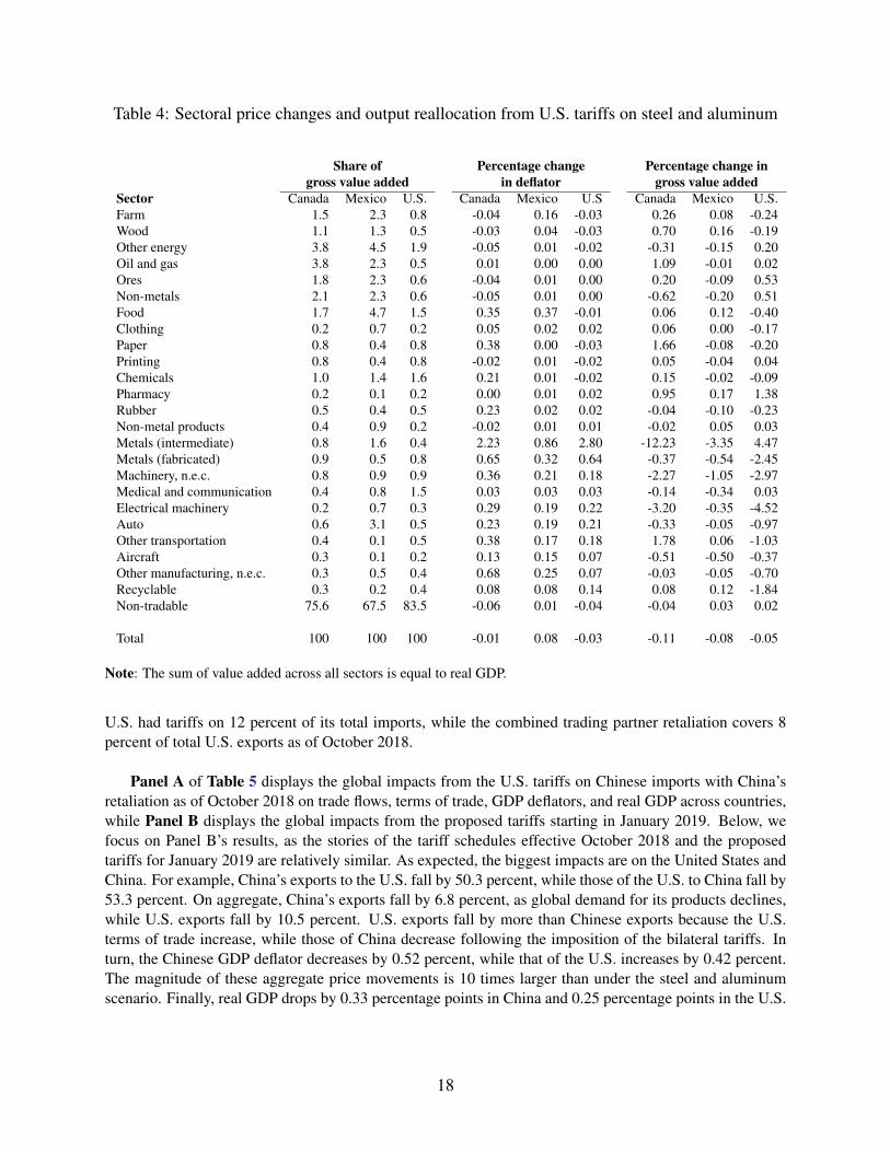
Table 4: Sectoral price changes and output reallocation from U.S. tariffs on steel and aluminum

Share of Percentage change Percentage change ingross value added in deflator gross value added

Sector Canada Mexico U.S. Canada Mexico U.S Canada Mexico U.S.Farm 1.5 2.3 0.8 -0.04 0.16 -0.03 0.26 0.08 -0.24Wood 1.1 1.3 0.5 -0.03 0.04 -0.03 0.70 0.16 -0.19Other energy 3.8 4.5 1.9 -0.05 0.01 -0.02 -0.31 -0.15 0.20Oil and gas 3.8 2.3 0.5 0.01 0.00 0.00 1.09 -0.01 0.02Ores 1.8 2.3 0.6 -0.04 0.01 0.00 0.20 -0.09 0.53Non-metals 2.1 2.3 0.6 -0.05 0.01 0.00 -0.62 -0.20 0.51Food 1.7 4.7 1.5 0.35 0.37 -0.01 0.06 0.12 -0.40Clothing 0.2 0.7 0.2 0.05 0.02 0.02 0.06 0.00 -0.17Paper 0.8 0.4 0.8 0.38 0.00 -0.03 1.66 -0.08 -0.20Printing 0.8 0.4 0.8 -0.02 0.01 -0.02 0.05 -0.04 0.04Chemicals 1.0 1.4 1.6 0.21 0.01 -0.02 0.15 -0.02 -0.09Pharmacy 0.2 0.1 0.2 0.00 0.01 0.02 0.95 0.17 1.38Rubber 0.5 0.4 0.5 0.23 0.02 0.02 -0.04 -0.10 -0.23Non-metal products 0.4 0.9 0.2 -0.02 0.01 0.01 -0.02 0.05 0.03Metals (intermediate) 0.8 1.6 0.4 2.23 0.86 2.80 -12.23 -3.35 4.47Metals (fabricated) 0.9 0.5 0.8 0.65 0.32 0.64 -0.37 -0.54 -2.45Machinery, n.e.c. 0.8 0.9 0.9 0.36 0.21 0.18 -2.27 -1.05 -2.97Medical and communication 0.4 0.8 1.5 0.03 0.03 0.03 -0.14 -0.34 0.03Electrical machinery 0.2 0.7 0.3 0.29 0.19 0.22 -3.20 -0.35 -4.52Auto 0.6 3.1 0.5 0.23 0.19 0.21 -0.33 -0.05 -0.97Other transportation 0.4 0.1 0.5 0.38 0.17 0.18 1.78 0.06 -1.03Aircraft 0.3 0.1 0.2 0.13 0.15 0.07 -0.51 -0.50 -0.37Other manufacturing, n.e.c. 0.3 0.5 0.4 0.68 0.25 0.07 -0.03 -0.05 -0.70Recyclable 0.3 0.2 0.4 0.08 0.08 0.14 0.08 0.12 -1.84Non-tradable 75.6 67.5 83.5 -0.06 0.01 -0.04 -0.04 0.03 0.02

Total 100 100 100 -0.01 0.08 -0.03 -0.11 -0.08 -0.05

Note: The sum of value added across all sectors is equal to real GDP.

U.S. had tariffs on 12 percent of its total imports, while the combined trading partner retaliation covers 8percent of total U.S. exports as of October 2018.

Panel A of Table 5 displays the global impacts from the U.S. tariffs on Chinese imports with China’sretaliation as of October 2018 on trade flows, terms of trade, GDP deflators, and real GDP across countries,while Panel B displays the global impacts from the proposed tariffs starting in January 2019. Below, wefocus on Panel B’s results, as the stories of the tariff schedules effective October 2018 and the proposedtariffs for January 2019 are relatively similar. As expected, the biggest impacts are on the United States andChina. For example, China’s exports to the U.S. fall by 50.3 percent, while those of the U.S. to China fall by53.3 percent. On aggregate, China’s exports fall by 6.8 percent, as global demand for its products declines,while U.S. exports fall by 10.5 percent. U.S. exports fall by more than Chinese exports because the U.S.terms of trade increase, while those of China decrease following the imposition of the bilateral tariffs. Inturn, the Chinese GDP deflator decreases by 0.52 percent, while that of the U.S. increases by 0.42 percent.The magnitude of these aggregate price movements is 10 times larger than under the steel and aluminumscenario. Finally, real GDP drops by 0.33 percentage points in China and 0.25 percentage points in the U.S.

18

Figure 2: Bilateral trade-weighted tariffs between the United States and China, by sector

Panel A: U.S. tariffs on Chinese goods imports

0%

10%

20%

30%

40%

50%

60%

Airc

raft

Auto

Chem

ical

s

Clot

hing

Elec

tric

al m

achi

nery

Farm

Food

Mac

hine

ry, n

.e.c

.

Med

ical

and

com

mun

icat

ion

Met

als (

fabr

icat

ed)

Met

als (

inte

rmed

iate

)

Non

-met

al p

rodu

cts

Non

-met

als

Oil

and

gas

Ore

s

Oth

er e

nerg

y

Oth

er m

anuf

actu

ring,

n.e

.c.

Oth

er tr

ansp

orta

tion

Pape

r

Phar

mac

y

Prin

ting

Recy

clab

le

Rubb

er

Woo

d

U.S. on China 2016 U.S. on China (10%) U.S. on China (25%)

Panel B: Chinese tariffs on U.S. goods imports

0%

10%

20%

30%

40%

50%

60%

Airc

raft

Auto

Chem

ical

s

Clot

hing

Elec

tric

al m

achi

nery

Farm

Food

Mac

hine

ry, n

.e.c

.

Med

ical

and

com

mun

icat

ion

Met

als (

fabr

icat

ed)

Met

als (

inte

rmed

iate

)

Non

-met

al p

rodu

cts

Non

-met

als

Oil

and

gas

Ore

s

Oth

er e

nerg

y

Oth

er m

anuf

actu

ring,

n.e

.c.

Oth

er tr

ansp

orta

tion

Pape

r

Phar

mac

y

Prin

ting

Recy

clab

le

Rubb

er

Woo

d

China on U.S. 2016 China on U.S. (10%) China on U.S. (25%)

19

Table 5: Global impacts from U.S. tariffs on $250 billion of Chinese goods imports(in percentage change)

Panel A: Tariffs effective October 2018Change in Trade Flows Terms of GDP Real

Exports to U.S. Exports to China Total Exports Total Imports Trade Deflator GDPAustralia 7.20 -7.96 -0.24 -0.29 -0.02 -0.08 -0.02Brazil 2.57 -4.71 -0.24 -0.26 0.00 0.01 0.00Canada -1.04 -6.07 -1.44 -1.43 0.00 0.16 -0.11China -36.99 · -5.16 -6.99 -0.14 -0.32 -0.26EU 4.30 -2.92 0.14 0.15 0.02 0.07 0.01India 1.42 -2.08 0.27 0.20 0.00 0.04 0.00Japan 7.15 -3.37 0.65 0.64 0.01 0.10 0.01Korea 7.28 -2.75 0.17 0.21 0.02 0.05 0.02Malaysia 15.91 -3.58 0.94 1.30 0.08 0.09 0.05Mexico 4.09 -9.18 1.76 1.76 0.09 0.54 0.02Norway 6.05 -2.83 0.05 0.06 0.00 0.06 0.00Peru 6.15 -9.19 0.15 0.15 -0.01 0.02 -0.01Switzerland 7.39 -4.04 0.18 0.18 0.00 0.10 0.00Thailand 10.78 -2.73 0.75 0.85 0.06 0.11 0.06U.S. · -43.73 -8.37 -5.08 0.04 0.25 -0.18ROW 2.91 -3.53 0.08 0.08 -0.01 0.02 0.00

Panel B: Proposed tariffs for January 2019Change in Trade Flows Terms of GDP Real

Exports to U.S. Exports to China Total Exports Total Imports Trade Deflator GDPAustralia 9.87 -11.52 -0.34 -0.40 -0.03 -0.13 -0.02Brazil 3.97 -6.95 -0.35 -0.39 -0.01 -0.01 -0.01Canada -0.36 -8.54 -1.25 -1.23 0.00 0.23 -0.11China -50.26 · -6.82 -9.24 -0.21 -0.52 -0.33EU 6.46 -4.30 0.19 0.19 0.02 0.08 0.02India 3.54 -3.06 0.50 0.36 0.01 0.04 0.01Japan 9.76 -4.69 0.85 0.83 0.02 0.11 0.02Korea 10.45 -3.82 0.24 0.29 0.03 0.05 0.02Malaysia 21.76 -4.99 1.27 1.75 0.11 0.10 0.07Mexico 5.86 -12.44 2.64 2.65 0.12 0.71 0.05Norway 7.65 -4.04 0.06 0.08 0.00 0.06 0.00Peru 7.37 -12.88 0.06 0.06 -0.02 0.00 -0.02Switzerland 10.12 -5.44 0.24 0.24 0.00 0.11 0.00Thailand 15.38 -3.88 1.03 1.17 0.09 0.14 0.08U.S. · -53.35 -10.45 -6.34 0.05 0.42 -0.25ROW 5.10 -5.10 0.11 0.11 0.00 0.01 0.00

Table 6 displays sectoral changes in U.S. exports to China and in Chinese exports to the U.S., togetherwith their current export shares. As the tariffs are broad-based across sectors, exports massively drop inalmost every sector except the ones for which there are no close import substitutes. This is clothing (and acouple of other smaller sectors) for Chinese exports to the U.S., and aircraft for U.S. exports to China.

The U.S.-China trade tensions also ripple through the global economy, especially among Canada, Mex-ico, and other Asian economies that either are part of the global supply chain affected by the tariffs or that

20

Table 6: Bilateral export reallocation from U.S. tariffs on $250 billion of Chinese goods imports(proposed tariff schedules starting in January 2019, with China’s retaliation)

Current exports from Change in exports from(as a share of exports) (in percent)

Sector China to U.S. U.S. to China China to U.S. U.S. to ChinaMedical and communication 34.0 16.3 -53.2 -55.2Clothing 15.1 0.7 -7.7 -31.3Other manufacturing, n.e.c. 12.7 1.8 -21.3 -43.8Machinery, n.e.c. 10.7 8.0 -91.0 -89.0Electrical machinery 6.5 4.5 -96.5 -94.0Rubber 4.1 4.9 -53.8 -63.2Metals (fabricated) 3.6 1.1 -79.3 -81.6Auto 2.9 9.3 -68.5 -63.0Chemicals 2.3 6.2 -40.6 -36.3Non-metal products 1.5 1.0 -37.0 -37.7Metals (intermediate) 1.4 3.1 -65.0 -75.3Food 1.2 4.7 -34.9 -35.5Wood 0.9 1.6 -90.3 -90.8Paper 0.7 1.9 -85.3 -61.4Other transportation 0.7 0.1 -83.5 -66.1Pharmacy 0.5 2.3 -7.9 -80.8Printing 0.5 1.2 -11.2 -71.9Farm 0.2 12.5 -19.7 -36.3Aircraft 0.2 11.9 -61.5 -4.6Oil and gas 0.1 1.4 -99.9 -98.5Non-metals 0.1 0.2 -15.8 -43.4Other energy 0.0 0.1 -47.9 -100.0Recyclable 0.0 3.9 -73.4 -37.0Ores 0.0 1.2 -12.0 -100.0

Total 100 100 -50.3 -53.3

offer close substitutes to Chinese and U.S. exports. Table 7 displays percentage changes in Canada, Mex-ico, U.S., and China sectoral exports, together with their current sectoral export shares. The table showsimportant export reallocations across these countries. For example, Canadian and Mexican exports go upin many export sectors that provide the U.S. with a close substitute to major Chinese export sectors (e.g.,clothing, medical and communication, electrical machinery, machinery, and other manufacturing constituteabout 80 percent of Chinese exports to the U.S.). In turn, these massive sectoral export reallocations haveimportant implications on prices and real economic activity.

Table 8 displays sectoral value added shares, sectoral price adjustments, and changes in sectoral realvalue added for the U.S., China, and the two other NAFTA partners. In the U.S., the sectors that experiencethe largest drop in Chinese imports see more noticeable increases in prices (e.g., clothing, medical and com-munication, electrical machinery, machinery, and other manufacturing), reflecting the lack of cheap inputsfrom China. In contrast, China’s output prices decline in almost every sector, reflecting the drop in aggregatedemand for Chinese products—as the Chinese economy relies heavily on its tradable sectors relative to theU.S. Overall, however, changes in sectoral prices remain relatively small, calling for a U.S. GDP deflatorincrease of 0.4 percentage point and Chinese GDP deflator decline of 0.5 percentage point. The sectoral out-

21

Table 7: Sectoral export reallocation from U.S. tariffs on $250 billion of Chinese goods imports(proposed tariff schedules starting in January 2019, with China’s retaliation)

Current exports from Change in exports from(as a share of total exports) (in percent)

Sector Canada Mexico U.S. China Canada Mexico U.S. ChinaFarm 5.4 3.7 5.2 0.6 -0.28 -0.88 -9.86 -0.43Wood 2.9 0.1 0.6 0.7 0.74 -6.37 -28.85 -14.90Other energy 1.8 0.0 0.7 0.1 -7.63 -37.94 -12.49 57.42Oil and gas 22.5 8.6 8.9 1.0 -0.87 -10.89 -5.46 12.54Ores 1.9 1.2 0.5 0.0 -8.62 -25.45 -22.49 32.71Non-metals 2.2 0.2 0.2 0.1 -0.40 -1.69 -2.43 0.48Food 6.9 4.2 6.1 2.0 0.22 -0.46 -5.94 -3.58Clothing 0.7 2.0 1.4 16.0 1.75 1.04 -2.86 -0.83Paper 3.6 0.5 1.8 0.9 0.35 -2.75 -10.22 -8.69Printing 0.3 0.3 0.8 0.4 -5.21 -2.98 -12.63 0.88Chemicals 3.5 2.1 7.3 3.8 0.22 -0.86 -4.04 -3.61Pharmacy 2.1 0.7 5.7 0.6 -4.38 -15.42 -9.79 15.24Rubber 3.9 2.6 5.5 4.0 5.05 1.87 -6.02 -8.42Non-metal products 0.7 1.0 1.0 2.2 3.12 0.96 -4.49 -3.58Metals (intermediate) 9.5 3.4 4.4 4.1 -22.16 -21.95 -25.98 -0.61Metals (fabricated) 1.2 1.7 1.9 3.8 2.01 -0.51 -19.26 -9.81Machinery, n.e.c. 5.3 7.9 11.1 9.2 7.20 7.66 -16.02 -14.87Medical and communication 2.8 19.0 12.0 27.8 12.43 15.30 -11.94 -10.33Electrical machinery 1.4 7.3 4.2 9.2 15.12 18.27 -20.19 -8.20Auto 14.8 28.4 9.4 2.6 1.60 0.93 -8.53 -13.88Other transportation 0.4 0.3 0.7 1.8 2.26 0.10 -17.23 -1.69Aircraft 3.6 0.6 6.0 0.2 -0.16 -0.97 -2.27 -9.88Other manufacturing, n.e.c. 1.8 3.8 3.4 8.7 5.81 4.75 -4.80 -5.06Recyclable 1.1 0.4 1.4 0.0 0.33 -2.65 -28.73 -7.74

Total 100 100 100 100 -1.25 2.64 -10.45 -6.82

put reallocation effects, however, are very large in some sectors. This is especially true for the economies ofCanada and Mexico, which experience large real output gains in many tradable sectors of their economies(e.g., medical and communication, and electrical machinery in Mexico). These sizable and broad sectoraloutput reallocations for the U.S. and its trading partners suggest important short-run price movements, asthey appear too large to be absorbed by the current industry structure due to the slow movements of laborand capital across sectors.

4.2 Endogenizing trade balancesAs in Caliendo and Parro (2015), the results in the previous subsection assumed that trade balances remainfixed following tariff changes. In the current context, however, this assumption may be misleading as thetrade rebalancing is at the root of the U.S.-led trade war. In this subsection, we endogenize trade balancesDn, by fixing income In in (27). That is,

22

Table 8: Sectoral price changes and output reallocationfrom U.S. tariffs on $250 billion of Chinese goods imports

(proposed tariff schedules starting in January 2019, with China retaliation)

Share of Percent change Percent change ingross value added in deflator gross value added

Sector Canada Mexico U.S. China Canada Mexico U.S China Canada Mexico U.S. ChinaFarm 1.5 2.3 0.8 6.6 0.21 0.78 0.33 -0.19 -0.04 -0.43 -3.30 -0.07Wood 1.1 1.3 0.5 4.4 0.21 0.71 0.45 -0.61 0.51 -0.36 -0.25 0.02Other energy 3.8 4.5 1.9 4.1 0.20 0.71 0.28 -0.61 -0.93 -1.12 -0.32 1.02Oil and gas 3.8 2.3 0.5 1.2 0.26 0.30 0.14 -0.26 -1.12 -11.16 -5.59 8.24Ores 1.8 2.3 0.6 1.3 0.21 0.73 0.35 -0.46 -3.09 -8.81 -2.30 9.77Non-metals 2.1 2.3 0.6 1.5 0.20 0.74 0.36 -0.61 -1.14 -0.87 -0.37 0.61Food 1.7 4.7 1.5 3.2 0.60 1.01 0.48 -0.37 0.05 0.04 -0.81 -0.40Clothing 0.2 0.7 0.2 2.5 -0.10 0.32 1.45 -0.51 0.83 0.30 -0.77 -0.33Paper 0.8 0.4 0.8 0.4 0.64 0.48 0.47 -0.30 1.72 -1.10 -0.38 -0.39Printing 0.8 0.4 0.8 0.4 0.24 0.60 0.38 -0.38 0.19 0.28 -0.61 0.42Chemicals 1.0 1.4 1.6 2.4 0.47 0.52 0.59 -0.37 0.35 -0.27 -1.08 -0.71Pharmacy 0.2 0.1 0.2 0.2 0.18 0.20 0.09 -0.32 -4.55 -14.40 -9.87 8.39Rubber 0.5 0.4 0.5 1.4 0.51 0.37 1.52 -0.28 3.45 1.07 -1.14 -1.84Non-metal products 0.4 0.9 0.2 2.0 0.20 0.61 1.24 -0.56 0.66 0.40 0.27 -0.65Metals (intermediate) 0.8 1.6 0.4 3.8 2.40 1.37 3.26 -0.48 -11.98 -2.58 3.29 -0.48Metals (fabricated) 0.9 0.5 0.8 1.1 0.84 0.65 1.56 -0.50 0.32 -0.10 0.42 -2.19Machinery, n.e.c. 0.8 0.9 0.9 3.4 0.63 0.43 1.62 -0.38 4.01 7.20 -4.53 -1.97Medical and communication 0.4 0.8 1.5 2.0 0.10 -0.01 2.40 0.05 7.43 15.31 1.41 -7.34Electrical machinery 0.2 0.7 0.3 1.7 0.49 0.20 2.50 -0.32 8.13 16.62 -4.55 -1.65Auto 0.6 3.1 0.5 1.8 0.76 0.57 1.04 -0.07 0.86 0.36 -3.85 -0.51Other transportation 0.4 0.1 0.5 0.5 0.64 0.54 0.96 -0.48 2.10 -0.81 -0.45 -0.49Aircraft 0.3 0.1 0.2 0.2 0.50 0.62 0.40 -0.06 -0.66 -1.58 -2.66 -0.23Other manufacturing, n.e.c. 0.3 0.5 0.4 1.3 0.70 0.18 2.56 0.46 3.53 4.56 -1.41 -5.49Recyclable 0.3 0.2 0.4 1.0 0.37 0.66 0.60 -0.17 0.27 1.19 -5.48 2.36Non-tradable 75.6 67.5 83.5 51.5 0.13 0.47 0.22 -0.42 0.01 0.46 0.00 -0.35

Total 100 100 100 100 0.23 0.71 0.42 -0.52 -0.11 0.05 -0.25 -0.33

Note: The sum of value added across all sectors is equal to real GDP.

κjni =1 + τ jni

′

1 + τ jni, and In = w′nLn +

J∑j=1

N∑i=1

τ jni′ πjni

′

1 + τ jni′Xjn′ +D′n. (27)

In line with Caliendo and Parro (2015)’s partial results, endogenizing trade balances does not changethe qualitative results.22 Table 9 displays the global impacts from the U.S. tariffs on Chinese imports withChina’s retaliation starting in January 2019 on trade flows, terms of trade, GDP deflators, real GDP, andtrade balances across countries. Indeed, the additional U.S. tariffs reduce the U.S. trade deficits and theChinese surplus, but the main takeaway is that endogenizing trade balances does not change the qualitativeresults displayed in section 4.1. Interestingly, the model suggests that Mexico (followed by Canada andJapan) experiences a relatively large improvement in its trade balance.

As we can see from Table 9, additional tariffs reduce both U.S. imports and U.S. exports, with littleimprovement in the U.S. trade deficit. As we pointed out earlier, the U.S. depends on imported inputs for

22Caliendo and Parro (2015) do not endogenize trade deficits, but instead compare results between fixed tradedeficits and balanced trade. Their results show little quantitative differences between the two. In later papers, Caliendoet al. (2017), Caliendo et al. (2018a), and Caliendo et al. (2018b) propose a way to endogenize trade balances. In thispaper, we use a simpler framework to endogenize trade balances at the cost of fixing income.

23

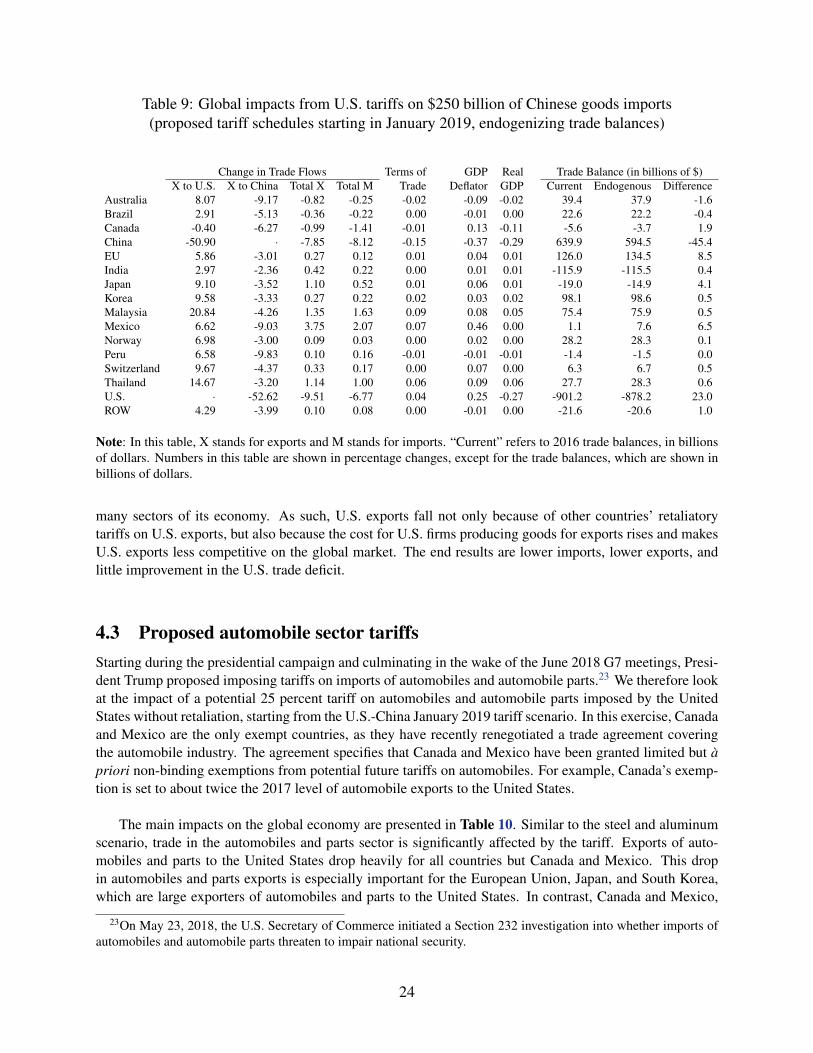
Table 9: Global impacts from U.S. tariffs on $250 billion of Chinese goods imports(proposed tariff schedules starting in January 2019, endogenizing trade balances)

Change in Trade Flows Terms of GDP Real Trade Balance (in billions of $)X to U.S. X to China Total X Total M Trade Deflator GDP Current Endogenous Difference

Australia 8.07 -9.17 -0.82 -0.25 -0.02 -0.09 -0.02 39.4 37.9 -1.6Brazil 2.91 -5.13 -0.36 -0.22 0.00 -0.01 0.00 22.6 22.2 -0.4Canada -0.40 -6.27 -0.99 -1.41 -0.01 0.13 -0.11 -5.6 -3.7 1.9China -50.90 · -7.85 -8.12 -0.15 -0.37 -0.29 639.9 594.5 -45.4EU 5.86 -3.01 0.27 0.12 0.01 0.04 0.01 126.0 134.5 8.5India 2.97 -2.36 0.42 0.22 0.00 0.01 0.01 -115.9 -115.5 0.4Japan 9.10 -3.52 1.10 0.52 0.01 0.06 0.01 -19.0 -14.9 4.1Korea 9.58 -3.33 0.27 0.22 0.02 0.03 0.02 98.1 98.6 0.5Malaysia 20.84 -4.26 1.35 1.63 0.09 0.08 0.05 75.4 75.9 0.5Mexico 6.62 -9.03 3.75 2.07 0.07 0.46 0.00 1.1 7.6 6.5Norway 6.98 -3.00 0.09 0.03 0.00 0.02 0.00 28.2 28.3 0.1Peru 6.58 -9.83 0.10 0.16 -0.01 -0.01 -0.01 -1.4 -1.5 0.0Switzerland 9.67 -4.37 0.33 0.17 0.00 0.07 0.00 6.3 6.7 0.5Thailand 14.67 -3.20 1.14 1.00 0.06 0.09 0.06 27.7 28.3 0.6U.S. · -52.62 -9.51 -6.77 0.04 0.25 -0.27 -901.2 -878.2 23.0ROW 4.29 -3.99 0.10 0.08 0.00 -0.01 0.00 -21.6 -20.6 1.0

Note: In this table, X stands for exports and M stands for imports. “Current” refers to 2016 trade balances, in billionsof dollars. Numbers in this table are shown in percentage changes, except for the trade balances, which are shown inbillions of dollars.

many sectors of its economy. As such, U.S. exports fall not only because of other countries’ retaliatorytariffs on U.S. exports, but also because the cost for U.S. firms producing goods for exports rises and makesU.S. exports less competitive on the global market. The end results are lower imports, lower exports, andlittle improvement in the U.S. trade deficit.

4.3 Proposed automobile sector tariffsStarting during the presidential campaign and culminating in the wake of the June 2018 G7 meetings, Presi-dent Trump proposed imposing tariffs on imports of automobiles and automobile parts.23 We therefore lookat the impact of a potential 25 percent tariff on automobiles and automobile parts imposed by the UnitedStates without retaliation, starting from the U.S.-China January 2019 tariff scenario. In this exercise, Canadaand Mexico are the only exempt countries, as they have recently renegotiated a trade agreement coveringthe automobile industry. The agreement specifies that Canada and Mexico have been granted limited but apriori non-binding exemptions from potential future tariffs on automobiles. For example, Canada’s exemp-tion is set to about twice the 2017 level of automobile exports to the United States.

The main impacts on the global economy are presented in Table 10. Similar to the steel and aluminumscenario, trade in the automobiles and parts sector is significantly affected by the tariff. Exports of auto-mobiles and parts to the United States drop heavily for all countries but Canada and Mexico. This dropin automobiles and parts exports is especially important for the European Union, Japan, and South Korea,which are large exporters of automobiles and parts to the United States. In contrast, Canada and Mexico,

23On May 23, 2018, the U.S. Secretary of Commerce initiated a Section 232 investigation into whether imports ofautomobiles and automobile parts threaten to impair national security.

24

Table 10: Global impact from proposed U.S. tariffs on automobiles and automobile parts(25 percent tariff on automobiles and automobile parts)

(in percentage change)

Exposure Exports of Total Terms of GDP RealAuto Exports Autos and Parts to Exports to Trade Deflator GDP

tariffs to U.S. U.S. World U.S. WorldAustralia 0.13 4.34 -59.95 -6.69 11.28 -0.48 -0.04 -0.20 -0.03Brazil 0.40 12.44 -60.18 -3.17 3.94 -0.53 -0.01 -0.04 -0.01Canada 13.84* 76.09 27.76 26.12 3.86 0.98 -0.01 0.50 -0.11China 0.59 17.53 -84.79 -17.87 -49.96 -6.81 -0.22 -0.58 -0.33EU 1.08 7.38 -59.17 -5.03 -0.54 -0.21 0.00 -0.02 0.00India 0.46 14.30 -60.20 -6.01 3.02 0.36 0.01 -0.01 0.01Japan 7.13 19.65 -58.85 -18.53 -8.79 -0.91 -0.02 -0.23 -0.02Korea 3.90 12.80 -59.97 -18.87 -6.02 -0.65 -0.09 -0.16 -0.07Malaysia 0.06 8.80 -59.69 -5.25 24.23 1.33 0.10 0.05 0.07Mexico 22.85* 80.75 27.55 22.69 11.74 5.74 0.24 1.35 0.18Norway 0.02 3.92 -59.75 -4.01 9.81 0.06 0.00 0.01 0.00Peru 0.02 15.72 -60.32 -9.12 9.38 -0.05 -0.04 0.01 -0.03Switzerland 0.07 10.30 -59.85 -7.17 11.18 0.23 0.00 0.06 0.00Thailand 0.37 10.81 -59.53 -2.04 16.03 0.99 0.08 0.06 0.08U.S. · · · -8.31 · -12.64 0.09 0.86 -0.37ROW 0.13 6.04 -59.38 -1.92 6.00 0.00 0.00 -0.05 0.01

Note: * Canada and Mexico are exempt under the new USMCA trade agreement. Without a trade agreement, Canada’sautomobiles and automobile parts tariff exposure would be 13.8 percent, while that of Mexico would be 22.9 percent.

whose automobiles and automobile parts markets are already well integrated with the United States, seetheir exports increase: Canada’s exports of automobiles and automobile parts to the United States increaseby 27.8 percent, while those of Mexico increase by 27.6 percent. Given reasonable annual growth rates inaddition to the increase in exports due to the tariffs, the current exemptions could become binding withina decade, long before the agreement is due to be renegotiated. The imposition of these tariffs would beparticularly beneficial for Mexico, whose marginal increase in real GDP growth would match the marginallosses of the United States. Despite a significant rise in exports, Canada would experience almost no changein real GDP growth. Outside of the United States, Japan and Korea would be most negatively affected.

The additional U.S. tariffs on automobiles and parts imports also have large impacts on prices, morethan doubling the growth in the GDP deflator for Canada, Mexico, and the United States. In particular, theimpact on sectoral prices is broad-based in the United States, having an important impact on both traded andnon-traded sectors. On aggregate, the model suggests an increase in the U.S. GDP deflator of 0.87 percent—compared with 0.42 percent in the U.S.-China January 2019 tariff scenario. In addition, the model suggestsan increase in the automobile sector deflator of 6.24 percent—from 1.04 under the U.S.-China January 2019tariff scenario.24 Considering an estimated average transaction price for light vehicles in the United States

24Most analysis reported estimates on the impacts of the proposed U.S. tariffs on automobiles and parts imports,including imports from Canada and Mexico. In this case, the impact on the U.S. GDP deflator increases to 1.24percent, while the automobile sector deflator increases by 12.49 percent when we also impose tariffs on the imports ofautomobiles and parts from Canada and Mexico.

25

of $37,007 in October 2018, the impacts of the tariffs sum up to an average increase of $2,310—which is inline with what has been reported by the media.25

5 ConclusionIn this paper, we build upon new developments in the international trade literature to identify and quan-tify the impact of tariff changes on the United States and the global economy. In particular, we apply themost recent data and trade elasticity estimates using the Ricardian model of Caliendo and Parro (2015) toquantify the impact of recently applied and proposed tariff changes. Overall, our results suggest that thenewly imposed and proposed tariff schemes imply considerable changes in trade flows and sectoral outputreallocations, but modest impacts on long-run aggregate prices and output levels. The size of the sectoraloutput reallocations suggests important short-run price movements, as they appear too large to be absorbedgiven the current industry structure due to the slow movements of labor and capital across sectors. Addi-tionally, endogenizing trade balances reduces the U.S. trade deficit and the Chinese surplus some, but themain takeaway is that it only marginally changes the results.

25Average transaction price for light vehicles in the United States as reported by Kelley Blue Book. Early mediacitations are reported in Lovely et al. (2018). In a July 2018 U.S. Commerce Department hearing, the NationalAutomobile Dealers Association estimated that a 25 percent tariff on automobiles and automobile parts would add$2,270 to the cost of U.S.-built cars, which is close to the estimate presented above.

26

ReferencesAmiti, Mary, Mi Dai, Robert C. Feenstra, and John Romalis, “How did China’s WTO entry benefit U.S.

prices?,” Staff Reports 817, Federal Reserve Bank of New York June 2017.

Anderson, Derek, Benjamin L Hunt, Mika Kortelainen, Michael Kumhof, Douglas Laxton, Dirk VMuir, Susanna Mursula, and Stephen Snudden, “Getting to Know GIMF: The Simulation Propertiesof the Global Integrated Monetary and Fiscal Model,” IMF Working Papers, International Monetary FundFebruary 2013.

Arkolakis, Costas, Arnaud Costinot, and Andres Rodrıguez-Clare, “New Trade Models, Same OldGains?,” American Economic Review, February 2012, 102 (1), 94–130.

Auer, Raphael, Barthlmy Bonadio, and Andrei A Levchenko, “The economics of revoking NAFTA,”BIS Working Papers 739, Bank for International Settlements August 2018.

Autor, David H., David Dorn, and Gordon H. Hanson, “The China Syndrome: Local Labor MarketEffects of Import Competition in the United States,” American Economic Review, October 2013, 103 (6),2121–68.

Bown, Chad P. and Melina Kolb, “Trumps Trade War Timeline: An Up-to-Date Guide,” Trade InvestmentPolicy Watch, Peterson Institute for International Economics 2018.

Caliendo, Lorenzo and Fernando Parro, “Estimates of the Trade and Welfare Effects of NAFTA,” TheReview of Economic Studies, 2015, 82 (1), 1–44.

, , Esteban Rossi-Hansberg, and Pierre-Daniel G. Sarte, “The impact of regional and sectoral pro-ductivity changes on the U.S. economy,” The Review of Economic Studies, 2018, 85 (4), 2042–2096.

, Luca David Opromolla, Fernando Parro, and Alessandro Sforza, “Goods and Factor Market Inte-gration: A Quantitative Assessment of the EU Enlargement,” NBER Working Papers 23695, NationalBureau of Economic Research August 2017.

, Maximiliano Dvorkin, and Fernando Parro, “Trade and Labor Market Dynamics: General Equilib-rium Analysis of the China Trade Shock,” Econometrica, 2018.

Corong, Erwin L., Thomas W. Hertel, Robert McDougall, Marinos E. Tsigas, and Dominique van derMensbrugghe, “The Standard GTAP Model, Version 7,” Journal of Global Economic Analysis, 2017, 2(1).

Costinot, Arnaud and Andres Rodrıguez-Clare, “Trade Theory with Numbers: Quantifying the Conse-quences of Globalization,” NBER Working Papers 18896, National Bureau of Economic Research March2014.

Dixit, Avinash K and Joseph E Stiglitz, “Monopolistic Competition and Optimum Product Diversity,”American Economic Review, 1977, 67 (3), 297–308.

Eaton, Jonathan and Samuel Kortum, “Technology, Geography, and Trade,” Econometrica, 2002, 70 (5),1741–1779.

Imbs, Jean and Isabelle Mejean, “Elasticity Optimism,” American Economic Journal: Macroeconomics,July 2015, 7 (3), 43–83.

27

International Monetary Fund, “World Economic Outlook,” Technical Report, International MonetaryFund October 2018.

Lovely, Mary E., Jeremy Cohen-Setton, and Euijin Jung, “Vehicular assault: proposed auto tariffs willhit American car buyers’ wallets,” Policy Brief, Peterson Institute for International Economics 2018.

Maggi, Giovanni, “International Trade Agreements,” Handbook of International Economics, Elsevier 2014.

Romalis, John, “NAFTA’s and CUSFTA’s Impact on International Trade,” The Review of Economics andStatistics, August 2007, 89 (3), 416–435.

Samuelson, Paul, “The Transfer Problem and Transport Costs, II: Analysis of Effects of Trade Impedi-ments,” The Economic Journal, 1954, 64 (254), 264–289.

Simonovska, Ina and Michael E. Waugh, “The elasticity of trade: Estimates and evidence,” Journal ofInternational Economics, 2014, 92 (1), 34–50.

Trefler, Daniel, “The Long and Short of the Canada-U. S. Free Trade Agreement,” American EconomicReview, September 2004, 94 (4), 870–895.

U.S. Department of Commerce, “The effect of imports of aluminum on the national security,” TechnicalReport, U.S. Department of Commerce January 2018.

, “The effect of imports of steel on the national security,” Technical Report, U.S. Department of Com-merce January 2018.

28

A Additional Tables and Results

Table A-1: Sector decomposition and corresponding ISIC

Number ISIC Sector1 01,05 Farm2 02,20 Wood3 10,12,23 Other energy4 11 Oil and gas5 13 Ores6 14 Non-metals7 15-16 Food8 17-19 Clothing9 21 Paper

10 22 Printing11 24 Chemicals12 2423 Pharmacy13 25 Rubber14 26 Non-metal products15 27 Metals (intermediate)16 28 Metals (fabricated)17 29 Machinery, n.e.c.18 30-33 Medical and communication19 31 Electrical machinery20 34 Auto21 351,352,359 Other transportation22 353 Aircraft23 36 Other manufacturing, n.e.c.24 37 Recyclable25 40-41 Electricity26 45 Construction27 50-52 Retail28 55 Hotels29 60 Land transport30 61 Water transport31 62 Air transport32 63 Aux transport33 64 Post34 65-67 Finance35 70 Real estate36 71 Renting machinery37 72 Computer38 73 Research and development39 74 Other business40 75 Public41 80 Education42 85 Health43 90-93 Other services44 95 Private

29

Table A-2: Shares of gross output versus gross value added

Share of Share ofgross output gross value added

Sector Canada Mexico U.S. China Canada Mexico U.S. ChinaFarm 1.5 2.2 1.0 3.6 1.5 2.3 0.8 6.6Wood 1.4 1.3 0.8 3.3 1.1 1.3 0.5 4.4Other energy 5.2 5.4 3.8 4.6 3.8 4.5 1.9 4.1Oil and gas 2.9 1.6 0.5 0.9 3.8 2.3 0.5 1.2Ores 1.4 1.6 0.6 0.9 1.8 2.3 0.6 1.3Non-metals 1.6 1.6 0.6 1.1 2.1 2.3 0.6 1.5Food 3.1 7.2 3.2 5.1 1.7 4.7 1.5 3.2Clothing 0.2 1.1 0.3 4.2 0.2 0.7 0.2 2.5Paper 0.9 0.5 1.1 0.6 0.8 0.4 0.8 0.4Printing 0.9 0.5 1.1 0.6 0.8 0.4 0.8 0.4Chemicals 1.5 2.8 2.5 4.2 1.0 1.4 1.6 2.4Pharmacy 0.2 0.2 0.3 0.3 0.2 0.1 0.2 0.2Rubber 0.8 0.8 0.7 2.7 0.5 0.4 0.5 1.4Non-metal products 0.5 1.0 0.3 3.1 0.4 0.9 0.2 2.0Metals (intermediate) 2.2 2.5 1.2 6.7 0.8 1.6 0.4 3.8Metals (fabricated) 1.1 0.9 1.2 1.8 0.9 0.5 0.8 1.1Machinery, n.e.c. 1.1 1.5 1.3 5.0 0.8 0.9 0.9 3.4Medical and communication 0.6 3.6 1.3 4.3 0.4 0.8 1.5 2.0Electrical machinery 0.3 1.4 0.4 3.4 0.2 0.7 0.3 1.7Auto 2.2 5.4 1.7 3.6 0.6 3.1 0.5 1.8Other transportation 0.6 0.1 0.7 0.7 0.4 0.1 0.5 0.5Aircraft 0.5 0.1 0.3 0.2 0.3 0.1 0.2 0.2Other manufacturing, n.e.c. 0.4 0.7 0.4 0.9 0.3 0.5 0.4 1.3Recyclable 0.4 0.4 0.4 0.7 0.3 0.2 0.4 1.0Non-tradables 68.7 55.5 74.4 37.5 75.6 67.5 83.5 51.5

Total 100 100 100 100 100 100 100 100

Note: This table shows the share differences between gross output and value added. Gross output is principally ameasure of sales or revenue from production for most industries, although it is measured as sales or revenue lesscost of goods sold for margin industries like retail and wholesale trade. Intermediate inputs are the foreign anddomestically produced goods and services used up by an industry in the process of producing its gross output. Valueadded is the difference between gross output and intermediate inputs and represents the value of labor (and capital)used in producing gross output. The sum of value added across all industries is equal to GDP for the economy. Inthis paper, we report the shares of gross value added as they are directly linked to the results on real GDP and GDPdeflators.

30

Table A-3: Sectoral gross output reallocation from U.S. tariffs on steel and aluminum

Share of Percentage change ingross output real gross output

Sector Canada Mexico U.S. Canada Mexico U.S.Farm 1.5 2.2 1.0 0.26 0.08 -0.24Wood 1.4 1.3 0.8 0.70 0.16 -0.19Other energy 5.2 5.4 3.8 -0.31 -0.15 0.20Oil and gas 2.9 1.6 0.5 1.09 -0.01 0.02Ores 1.4 1.6 0.6 0.20 -0.09 0.53Non-metals 1.6 1.6 0.6 -0.62 -0.20 0.51Food 3.1 7.2 3.2 0.06 0.12 -0.40Clothing 0.2 1.1 0.3 0.06 0.00 -0.17Paper 0.9 0.5 1.1 1.66 -0.08 -0.20Printing 0.9 0.5 1.1 0.05 -0.04 0.04Chemicals 1.5 2.8 2.5 0.15 -0.02 -0.09Pharmacy 0.2 0.2 0.3 0.95 0.17 1.38Rubber 0.8 0.8 0.7 -0.04 -0.10 -0.23Non-metal products 0.5 1.0 0.3 -0.02 0.05 0.03Metals (intermediate) 2.2 2.5 1.2 -12.23 -3.35 4.47Metals (fabricated) 1.1 0.9 1.2 -0.37 -0.54 -2.45Machinery, n.e.c. 1.1 1.5 1.3 -2.27 -1.05 -2.97Medical and communication 0.6 3.6 1.3 -0.14 -0.34 0.03Electrical machinery 0.3 1.4 0.4 -3.20 -0.35 -4.52Auto 2.2 5.4 1.7 -0.33 -0.05 -0.97Other transportation 0.6 0.1 0.7 1.78 0.06 -1.03Aircraft 0.5 0.1 0.3 -0.51 -0.50 -0.37Other manufacturing, n.e.c. 0.4 0.7 0.4 -0.03 -0.05 -0.70Recyclable 0.4 0.4 0.4 0.08 0.12 -1.84Non-tradable 68.7 55.5 74.4 -0.06 0.03 0.01

Total 100 100 100 -0.31 -0.11 -0.07

31

Table A-4: Sectoral gross output reallocationfrom U.S. tariffs on $250 billion of Chinese goods imports

(proposed tariff schedules starting in January 2019, with China retaliation)

Share of Percentage change ingross output real gross output

Sector Canada Mexico U.S. China Canada Mexico U.S. ChinaFarm 1.5 2.2 1.0 3.6 -0.04 -0.43 -3.30 -0.07Wood 1.4 1.3 0.8 3.3 0.51 -0.36 -0.25 0.02Other energy 5.2 5.4 3.8 4.6 -0.93 -1.12 -0.32 1.02Oil and gas 2.9 1.6 0.5 0.9 -1.12 -11.16 -5.59 8.24Ores 1.4 1.6 0.6 0.9 -3.09 -8.81 -2.30 9.77Non-metals 1.6 1.6 0.6 1.1 -1.14 -0.87 -0.37 0.61Food 3.1 7.2 3.2 5.1 0.05 0.04 -0.81 -0.40Clothing 0.2 1.1 0.3 4.2 0.83 0.30 -0.77 -0.33Paper 0.9 0.5 1.1 0.6 1.72 -1.10 -0.38 -0.39Printing 0.9 0.5 1.1 0.6 0.19 0.28 -0.61 0.42Chemicals 1.5 2.8 2.5 4.2 0.35 -0.27 -1.08 -0.71Pharmacy 0.2 0.2 0.3 0.3 -4.55 -14.40 -9.87 8.39Rubber 0.8 0.8 0.7 2.7 3.45 1.07 -1.14 -1.84Non-metal products 0.5 1.0 0.3 3.1 0.66 0.40 0.27 -0.65Metals (intermediate) 2.2 2.5 1.2 6.7 -11.98 -2.58 3.29 -0.48Metals (fabricated) 1.1 0.9 1.2 1.8 0.32 -0.10 0.42 -2.19Machinery, n.e.c. 1.1 1.5 1.3 5.0 4.01 7.20 -4.53 -1.97Medical and communication 0.6 3.6 1.3 4.3 7.43 15.31 1.41 -7.34Electrical machinery 0.3 1.4 0.4 3.4 8.13 16.62 -4.55 -1.65Auto 2.2 5.4 1.7 3.6 0.86 0.36 -3.85 -0.51Other transportation 0.6 0.1 0.7 0.7 2.10 -0.81 -0.45 -0.49Aircraft 0.5 0.1 0.3 0.2 -0.66 -1.58 -2.66 -0.23Other manufacturing, n.e.c. 0.4 0.7 0.4 0.9 3.53 4.56 -1.41 -5.49Recyclable 0.4 0.4 0.4 0.7 0.27 1.19 -5.48 2.36Non-tradable 68.7 55.5 74.4 37.5 0.05 0.71 0.05 -0.58

Total 100 100 100 100 -0.17 0.85 -0.28 -0.71

32

B Data

B.1 Bilateral trade flowsWe use bilateral trade flow data from the United Nations Statistical Division (UNSD) Commodity Trade(COMTRADE) database. We take an average of the values from 2014 and 2015 for each of the 16 countriesand areas in our sample. We create a representative European Union by combining COMTRADE data foreach of the 28 member states. We also create a representative rest of world (ROW) by taking the combinedtrade value between a country and all its partners in our sample, and subtracting it from the trade valuebetween this country and the entire world (as reported in the COMTRADE database). Trade flow valuesare reported in U.S. dollars at current prices and include cost, insurance and freight (CIF). Commodities aredefined using the 2012 Harmonized Commodity Description and Coding System (HS), at a six-digit levelof aggregation. We concord the HS12 data to ISIC Revision 3 at a two-digit level of aggregation by firstusing the Bank of Canada’s concordance table purchased from Statistics Canada to map HS12 to NAPCS.We then manually map the NAPCS codes to ISIC Revision 3 for the sectors of interest, which can be foundin Table A-1.

B.2 TariffsWe use bilateral tariff data at the sectoral level from the World Trade Organization (WTO) Tariffs DownloadFacility, for the year 2016. We select 2016 (HS 12) tariffs for the reporting country of interest, and selectproducts reported using the same HS 12 classification at a six-digit level of aggregation. We construct atariff matrix for each country by first applying any existing trade agreement that is in place. We apply theseagreements to the HS code only if the tariff rate is less than the most-favored-nation (MFN) tariff rate. Iftrade agreement data are not available in a country due to a reporting issue, we apply reciprocity across theseagreements. For example, Mexico does not report any agreements; therefore, we apply reciprocity to ensurethat NAFTA tariff rates between Mexico, Canada, and the United States are accurate. We weight each tariffmatrix against the average bilateral trade values for 2014 and 2015, as noted above. We create the ROWtariff matrix by combining the MFN tariff rates for each country/area in our sample and then weighting itagainst average ROW trade values.

B.3 Value added and gross productionWe use gross output and value added data at the sectoral level from the OECD input-output tables, for theyear 2011. We use 2011 data because at the time of publication, this is the most up-to-date data that theOECD provides that can give us consistency across countries and concepts. We create gross output and valueadded data for the European Union by combining values from each of the 28 member states. We create grossoutput and value added data for the ROW by combining values from the remaining countries in the databasethat are not in our sample (including an OECD-built ROW). The value added and gross output data fromthe OECD are reported in millions of U.S. dollars. For a few sectors in our sample, we split sectoral grossoutput and value added data to align with our list of sectors in Table A-1. For example, we split the grossoutput and value added sector 21-22 data evenly to create our sector 21 (paper) and sector 22 (printing).

B.4 Input-output tables and intermediate consumptionWe construct the share of intermediate inputs from each sector in sectoral gross output, using informationfrom the OECD Input-Output Database for 2011. We create the European Union Input-Output table by

33

combining values from each of the 28 member states. We create the Rest of World Input-Output table bycombining values from the remaining countries in the database that are not in our sample. Like the valueadded and gross output data, we must split certain sectors to match our list of sectors in Table A-1.

B.5 Estimation of dispersion of productivityWe estimate the dispersion of productivity following Caliendo and Parro (2015) and using equation (26).We use all trade and tariff data used in the model calibration, while removing some outliers in specific cases,which we list here. For each sector, we remove a country if its share of exports in that sector is less than 0.1%of global exports. We also remove Switzerland from all sectors since its tariffs are set to zero. In addition,we remove Malaysia from the clothing and other manufacturing sectors, Peru from the printing, machineryn.e.c., auto and other manufacturing sectors, and Norway, Thailand, Brazil, and India from the auto sector.These represent outliers in our estimates. Estimates are robust to the removal of other observations.

34

C Timeline of Additional TariffsBelow is a detailed timeline of additional tariffs. Official releases from the United States and its tradingpartners containing HS tariff lines are hyperlinked in the text. These are the additional tariffs, quotas, andexemptions that have been incorporated in the scenarios discussed in section 4. Bown and Kolb (2018) atthe Peterson Institute for International Economics provide an excellent timeline of events.

C.1 Steel and aluminum tariffs• March 8, 2018: The United States formally announces steel and aluminum tariffs, along with tempo-

rary exemptions for Canada and Mexico.

– Steel proclamation– Aluminum proclamation

• March 22, 2018: The United States announces additional steel and aluminum tariff temporary exemp-tions.

– Additional steel proclamation– Additional aluminum proclamation

• March 23, 2018: The United States steel and aluminum tariffs go into effect.

• March 28, 2018: South Korea agrees to an absolute quota that reduces steel exports to the UnitedStates, in return for a permanent exemption from the steel tariffs announced on March 8, 2018.

• April 2, 2018: In response to the U.S. steel and aluminum tariffs, China imposes retaliatory tariffs onUnited States products such as aluminum waste, pork, fruits, and nuts. A 25% tariff will be levied onaluminum waste and scrap, and pork products, while a 15% tariff will be levied on other products.

– China retaliatory list

• April 30, 2018: The United States signs a proclamation that extends the steel and aluminum tariffexemptions for the European Union, Canada, and Mexico until June 1, 2018.

• June 1, 2018: The United States signs a proclamation that ends the steel and aluminum tariff exemptionfor Canada, Mexico, and the European Union. The proclamation also outlines the details of quotasnegotiated by Argentina, Brazil, and South Korea with the United States. These quotas restrict steeland aluminum exports to the United States, in exchange for tariff exemptions.

• June 22, 2018: In response to the U.S. steel and aluminum tariffs, the European Union imposesretaliatory tariffs on United States products such as steel and aluminum, agriculture, and food.

– European Union retaliatory list

• July 1, 2018: In response to the U.S. steel and aluminum tariffs, Canada imposes retaliatory tariffs of25% on steel imports, and 10% on aluminum and a variety of other imports from the United States.

– Canada retaliatory list

35

• July 5, 2018: In response to the U.S. steel and aluminum tariffs, Mexico imposes retaliatory tariffs onUnited States products such as pork and whiskey.

– Mexico retaliatory list

• In addition, the United States increases the steel and aluminum tariff rates for Turkey, and Russia andTurkey impose retaliatory tariffs on U.S. imports. These tariffs are not accounted for because they arepart of the rest of the world region.

• Finally, we leave out India and Japan because they have not officially imposed retaliatory tariffs. Theyhave simply announced their intention to impose them. India retaliatory tariffs will take effect on De-cember 17, 2018. We would not account for India’s retaliatory tariffs anyway, because they are part ofthe rest of the world region.

C.2 U.S.-China trade tension• June 6, 2018: China and the United States impose first phase of the June 15 tariffs.

– The United States imposes the first phase of its $50 billion tariff plan on Chinese imports, whichincludes applying tariffs to $34 billion worth of Chinese products.

– China also imposes the first phase of its $50 billion tariff plan on United States imports, whichincludes applying tariffs on $34 billion worth of U.S. products.

• August 23, 2018: China and the United States impose second phase of the June 15 tariffs.

– The United States imposes the second phase of its $50 billion tariffs plan on Chinese imports,which includes applying tariffs to the remaining $16 billion worth of Chinese products.

– China also imposes the second phase of its $50 billion tariff plan on U.S. imports, applying tariffson the remaining $16 billion worth of U.S. products.

• September 24, 2018: China and the United States impose third phase of tariffs.

– The United States imposes new tariffs on $200 billion worth of Chinese imports, originally an-nounced on September 17. The list of Chinese imports are subject to a 10% tariff from September24, 2018 to December 31, 2018, and will be subject to a 25% tariff beginning on January 1, 2019.

– China also imposes new tariffs on $60 billion worth of U.S. imports, originally announced onSeptember 18. The U.S. imports are subject to tariffs ranging from 5 to 10 percent until January1, 2019.∗ China retaliatory list of U.S. imports at 5 percent∗ China retaliatory list of U.S. imports at 10 percent∗ China retaliatory list of U.S. imports at 20 percent∗ China retaliatory list of U.S. imports at 25 percent

C.3 Proposed automobiles and automobile parts tariffsFor this scenario, we impose a 25 percent tariff on all U.S. imported automobiles and automobile parts(worth about $350 billion). This is the tariffs assumption used in the Fall 2018 World Economic Outlook(International Monetary Fund (2018)), without trading partner retaliation.

36