the thermodynamic approach to electromagnetic dissipation ... · the thermodynamic approach to...
TRANSCRIPT

The Thermodynamic Approach toElectromagnetic Dissipation and Forces
Mario Liu 1
Institut fur Theoretische Physik, Universitat Tubingen,72076 Tubingen, Germany, EC
andKlaus Stierstadt 2
Sektion Physik, Universitat Munchen,
80539 Munchen, Germany, EC
May 12, 2005
1email: [email protected] is limited to chapter
gene2gene22 and section
highhigh3.1.

Abstract
There is a thermodynamic approach to macroscopic electrodynamics that is rig-oros, powerful, and above all, simple. Although it provides unambiguous an-swers to many questions, including conceptually subtle ones about dissipationand forces, this view point is little known, and even less taught. This articlepresents a thorough yet pedagogical review on this subject.

Contents
1 Introduction 31.1 Coarse-Graining Revisited . . . . . . . . . . . . . . . . . . . . . . 41.2 The Key Role of Locality . . . . . . . . . . . . . . . . . . . . . . . 81.3 Electro- and Magnetostatics . . . . . . . . . . . . . . . . . . . . . 91.4 Electrodynamics . . . . . . . . . . . . . . . . . . . . . . . . . . . 111.5 Content of this Article . . . . . . . . . . . . . . . . . . . . . . . . 12
2 Stress and Force in Equilibrium 142.1 Derivation of the Stress . . . . . . . . . . . . . . . . . . . . . . . . 15
2.1.1 Electric Contributions . . . . . . . . . . . . . . . . . . . . 162.1.2 Magnetic Contributions . . . . . . . . . . . . . . . . . . . 182.1.3 Conclusions and Comparisons . . . . . . . . . . . . . . . . 19
2.2 Bulk Force Density and Equilibria . . . . . . . . . . . . . . . . . . 202.2.1 True Equilibrium . . . . . . . . . . . . . . . . . . . . . . . 212.2.2 Quasi-Equilibrium . . . . . . . . . . . . . . . . . . . . . . 222.2.3 Gravitation . . . . . . . . . . . . . . . . . . . . . . . . . . 23
2.3 The Surface Force Density . . . . . . . . . . . . . . . . . . . . . . 232.3.1 Stress in Equilibrium . . . . . . . . . . . . . . . . . . . . . 232.3.2 Boundary Conditions . . . . . . . . . . . . . . . . . . . . . 252.3.3 The Total Surface Force . . . . . . . . . . . . . . . . . . . 26
2.4 Zero-Field Pressure and the Kelvin Force . . . . . . . . . . . . . . 282.4.1 Different Zero-Field Pressures . . . . . . . . . . . . . . . . 292.4.2 Different Kelvin Forces . . . . . . . . . . . . . . . . . . . . 312.4.3 The Magnetic Bernoulli Equation . . . . . . . . . . . . . . 31
2.5 Equilibrium Experiments . . . . . . . . . . . . . . . . . . . . . . . 322.5.1 Field Induced Variations in Densities . . . . . . . . . . . . 322.5.2 Current Carrying Vertical Wire . . . . . . . . . . . . . . . 332.5.3 Hydrostatics in the Presence of Fields . . . . . . . . . . . . 332.5.4 Magnetic O-Rings and Scrap Separation . . . . . . . . . . 35
3 Dissipative Electrodynamics 383.1 Rarefied Plasmas . . . . . . . . . . . . . . . . . . . . . . . . . . . 39
3.1.1 The Eulerian Newtonian Equation . . . . . . . . . . . . . 39
1

3.1.2 The Field Contributions . . . . . . . . . . . . . . . . . . . 403.1.3 Energy and Momentum Conservation . . . . . . . . . . . . 41
3.2 Weakly Dissociated Liquids . . . . . . . . . . . . . . . . . . . . . 413.2.1 The Material Contributions . . . . . . . . . . . . . . . . . 413.2.2 The Field Contributions . . . . . . . . . . . . . . . . . . . 433.2.3 The 2-field Theory . . . . . . . . . . . . . . . . . . . . . . 443.2.4 Radiation Damping . . . . . . . . . . . . . . . . . . . . . . 46
3.3 The Hydrodynamic Maxwell Theory . . . . . . . . . . . . . . . . 463.3.1 Frame-Independent Thermodynamics . . . . . . . . . . . . 463.3.2 Reactive Terms . . . . . . . . . . . . . . . . . . . . . . . . 493.3.3 Dissipative Terms . . . . . . . . . . . . . . . . . . . . . . . 503.3.4 Relevance of the Results . . . . . . . . . . . . . . . . . . . 513.3.5 The Total Momentum Density . . . . . . . . . . . . . . . . 53
3.4 Off-Equilibrium Experiments . . . . . . . . . . . . . . . . . . . . . 533.4.1 Incompatible Equilibria . . . . . . . . . . . . . . . . . . . 543.4.2 Rotational Field deflection . . . . . . . . . . . . . . . . . . 563.4.3 Field-Enhanced Viscosity . . . . . . . . . . . . . . . . . . . 573.4.4 Dissipative Magnetic Surface Force . . . . . . . . . . . . . 57
3.5 Higher Frequencies . . . . . . . . . . . . . . . . . . . . . . . . . . 58
4 Conclusion 60
A Legendre Transformation of Field Variables 61
2

Chapter 1
Introduction
The microscopic Maxwell theory1, being the epitome of simplicity and stringency,strikes some as the mathematical equivalent of the divine ordinance: “Let therebe light.” The macroscopic version of it is not held in similar esteem, and farless physicists are willing to accept it as an equally important pillar of modernphysics. At the start of his lectures on electrodynamics, a colleague of mineroutinely asserts, only half in jest, that the fields D and H were invented byexperimentalists, with the mischievous intent to annoy theorists. He then goeson with his lectures, without ever mentioning these two letters again.
Even if this is an extreme position, his obvious vexation is more widely shared.Both to novices and some seasoned physicists, the macroscopic Maxwell the-ory seems quietly obscure, only precariously grasped. More moderate colleaguesmaintain, in a similar vein, that of the four macroscopic fields, only E, B arefundamental, as they are the spatially averaged microscopic fields, 〈e〉, 〈b〉. Con-taining information about the polarization P and magnetization M , the fields D,H are part of the condensed system, and hence rather more complex quantities.Although subscribed to by many, this view contains some disturbing ramifications– one being that this obviously basic difference seems to be of little consequences,and it is something as humdrum as the orientation of the system’s surface withrespect to the external field Eex, which decides whether D or E is to assume thevalue of Eex. Others are considered below.
The characteristic distinction between micro- and macroscopic theories is thetime-inversion symmetry: Microscopic equations of motion are reversible, theynever contain dissipative terms. Macroscopic theories are always irreversible,they would be incomplete without them. (Some equations in particle physicsare CPT-invariant – this is then what the associated macro-equations, shouldthey ever be needed, will break.) In the Maxwell theory, dissipation is usuallyaccounted for by the imaginary part of the dielectric function ε and permeability2
1Part of the introduction is similar in content to a popular article in German, which appearedin the Dec/2002 issue of Physik Journal.
2The permeability µm is given a superscript, because we need the bare µ to denote the
3

µm. This is not generally valid, as it works only for weak fields, when ε and µm
are field-independent. Besides, there are circumstances (as we shall see) in whichdissipation is accounted for by the real part of ε or µm.
A further thorny subject is that of the electromagnetic force. The microscopicMaxwell equations are linear and may be directly averaged. This is different forthe force, for which even the microscopic expression is nonlinear. As a result,macroscopic electromagnetic force is notorious for being a difficult subject, andhas been a consistent source of confusion and controversy. Yet should not astudent of physics, close to his finals, know as a matter of course the expressionfor the electromagnetic force felt by a neutral, polarizable body?
After all the course work is done, even a good student must have the impres-sion that electrodynamics and thermodynamics, two areas of classical physics,are completely separate subjects. The word entropy does not appear once in thehundreds of pages of Jackson’s classics on electrodynamics
jackson[1]. Yet, based on con-
cepts as primary as overwhelming probability, thermodynamic considerations arethe bedrock of macroscopic physics, so general there can be little doubt that theymust also hold for charges, currents and fields. The success London, Ginzburgand Landau enjoyed in understanding superconductivity is one proof that this istrue. As we shall see, simple thermodynamic considerations are indeed useful forunderstanding macroscopic electrodynamics, including subjects such as structureof the Maxwell equations, constitutive relations, field dissipation, and electro-magnetic forces. Some of these could easily be taught in introductory courses,and would usefully be part of the common knowledge shared by all physicists.
In the rest of the introduction, we take a closer look, discussing first the usualderivation of macroscopic electrodynamics employing coarse-graining, clarifyingits basic ideas and pinpointing its difficulties. Then the thermodynamic approachis introduced, making three simple, useful, and possibly surprising points: • It isthe introduction of fields that renders the description of electromagnetism local.• The static Maxwell equations are merely an expression of the entropy beingmaximal in equilibrium. • The structure of the temporal Maxwell equationsfollows from charge conservation alone.
1.1 Coarse-Graining Revisited
It was Lorentz who first differentiated between two versions of the Maxwell equa-tions: The microscopic ones with two fields and the macroscopic ones with four.He also showed how to obtain the latter from the former, a derivation that is con-ceptually helpful to be divided into two steps: The first consists only of algebraicmanipulations, the second, crossing the Rubicon to macroscopics and irreversibil-
chemical potential, a quantity we shall often consider.
4

ity, is the conceptually subtle one. Starting from the microscopic equations,
∇ · e = ρe, ∇ · b = 0, (1.1) m1
e = c∇ × b − je, b = −c∇ × e, (1.2) m2
we divide the charge and current into two parts, ρe = ρ1 + ρ2, je = j1 + j2
(typically taking 1 as free and 2 as bound, though this is irrelevant at the mo-ment). Next, to eliminate ρ2, j2, the fields p, m are introduced: ρ2 = −∇ · p,j2 = −(p+c∇×m). Although not unique, this step is always possible if ρ2 is con-served – the fields’ definitions imply ρ2 +∇ ·j2 = 0. Finally, defining h ≡ b−m,d ≡ e + p eliminates p, m and effectuates the “macroscopic” appearance:
∇ · d = ρ1, ∇ · b = 0, (1.3) M1
d = c∇ × h − j1, b = −c∇ × e. (1.4) M2
Although seemingly more complicated, Eqs (M1M11.3,
M2M21.4) are equivalent to (
m1m11.1,
m2m21.2)
and not at all macroscopic. This ends the first of the two steps.Next, we coarse-grain these linear equations, spatially averaging them over
a small volume – call it grain – repeating the process grain for grain till thegrains fill the volume. Denoting the coarse-grained fields as EM ≡ 〈e〉, D ≡ 〈d〉,B ≡ 〈b〉, HM ≡ 〈h〉, P ≡ 〈p〉, M ≡ 〈m〉, ρε ≡ 〈ρ1〉, jε ≡ 〈j1〉, the seeminglyobvious result is the macroscopic Maxwell equations,
∇ · D = ρε, ∇ · B = 0, (1.5) M3
D = c∇ × HM − jε, B = −c∇ × EM . (1.6) M4
[The superscript M may appear whimsical here, but will be seen as sensible soon.It denotes the two fields appearing only in the temporal Maxwell equations (
M4M41.6).]
The sketched derivation leads directly to the conclusion that EM , B are theaveraged microscopic fields, while D, HM are complicated by P , M . Identifyingthe latter (to leading orders) with the electric and magnetic dipole densities,respectively, and employing linear response theory, imply a host of consequences,of which the presently relevant one is: D, HM are functions of EM , B – pairwiseproportional for weak fields, with a “temporally nonlocal dependence.” In otherwords, D depends also on the values of EM a while back, and HM on B. This iseasily expressed in Fourier space, D = ε(ω)EM , HM = B/µm(ω), where ε, µm arecomplex functions of the frequency ω. [A field with tilde denotes the respectiveFourier component, eg. D(t) =
∫dωD(ω)e−iωt/2π.] One cannot overestimate the
importance of these two constitutive relations. They determine D, HM in termsof EM = 〈e〉, B = 〈b〉, dispense with the above mentioned non-uniqueness, closethe set of equations for given sources, and introduce dissipation.
General considerations (including especially causality) show the real part ofε to be even in ω, and the imaginary part odd. Focusing on slow processesin dielectrics, we expand ε in the frequency ω to linear order, writing D =
5

ε(1 + iωβε)EM , where ε, β are real, frequency-independent material parameters.Transformed back into temporal space, the constitutive relation reads
D = ε(EM − βεEM
). (1.7) 20-1
This is a succinct formula: The temporal non-locality is reduced to the depen-dence on EM ; and we intuitively understand that this term (imaginary in Fourierspace) is dissipative, as it resembles the damping term ∼ x in the pendulumequation, in which the restoring force is ∼ x. (Stability requires ε > 0, and β ispositive if electromagnetic waves are to be damped.)
The microscopic Maxwell equations (m1m11.1,
m2m21.2) are invariant under time rever-
sal: If e(t), b(t) are a solution, so are e(−t), −b(−t). All microscopic variablespossess a “time reversal parity.” If even, the variable stays unchanged under timereversal, if odd, it reverses its sign. (A particle’s coordinate is even, its velocityodd.) Stipulating e as even and b as odd, the invariance of the Maxwell equationsstems from the fact that each of Eqs (
m1m11.1,
m2m21.2) contains only terms with the same
parity, eg. the first of Eqs (m2m21.2) contains only odd terms: e, ∇ × b, and je.
As mentioned, macroscopic theories are never invariant under time reversal,and a solution running backwards in time does not remain one. This is universallyachieved by insisting on a unique time reversal parity for the variables, yet takingthe equations of motion as mixtures of odd and even terms. In the case of themacroscopic Maxwell equations, we take the variable EM = 〈e〉 as even, andB = 〈b〉 as odd, because averaging only reduces a strongly varying field to itsenvelope, with the parity remaining intact. D, on the other hand, given byEq (
20-120-11.7), is a mixture of terms with different parities. When inserted into the
Maxwell equations, it destroys the reversibility.Unfortunately, these results are only valid for linear constitutive relations.
Attempt to generalize them to higher-order terms is met with swiftly growingcomplications, creating the impression that dissipation in strongly non-linear sys-tems does not possess a simple description. In addition, there is a grave problemeven with the linear constitutive relation: Eq (
20-120-11.7) cannot be right, because it
contains the unphysical, exploding solution: D(t) = D0 and
EM(t) = EM0 exp(t/βε) ≡ EM
0 exp(t/τ), (1.8)
for the initial conditions D = D0, EM = EM
0 at t = 0.This solution is avoided by inverting the constitutive relation, EM = D/ε(ω),
which upon expansion becomes EM = (1/ε− iωβ)D, or back in temporal space,
EM = D/ε + βD. (1.9) 21-1
Now EM depends on D, D, and although there is still a solution D ∼ exp(−t/τ),it relaxes toward zero and is benign. The above frequency expansion confines thevalidity of Eqs (
20-120-11.7,
21-121-11.9) to coarse temporal resolutions, for which a relaxing mode
6

vanishes, but not an exploding one. Only Eq (21-121-11.9) can be correct. Because of an
analogous instability, HM ∼ et/µmα, the proper magnetic constitutive relation is
HM = B/µm + αB. (1.10) 21a
Given Eq (21-121-11.9,
21a21a1.10), the fields D, B are clearly the simple, and EM , HM the
composite, quantities – and presumably D is even, B odd, while EM , HM lack aunique parity? In fact, the reason for taking D as even is just as persuasive astaking EM , because neither the algebraic manipulations (defining d from e, ρ2),nor the ensuing spatial averaging could possibly have altered D’s parity: Eqs (
M1M11.3,
M2M21.4) are reversible and retain the invariance of Eqs (
m1m11.1,
m2m21.2).
There is nothing wrong with rewriting the microscopic Maxwell equationsas Eqs (
M1M11.3,
M2M21.4) and averaging them to obtain Eqs (
M3M31.5,
M4M41.6). But these are
reversible and not yet the macroscopic Maxwell equations. In fact, the basic rea-son dissipative terms appear is because the constitutive relations, D = ε(ω)EM
and HM = B/µm(ω), close the Maxwell equations, rendering the dynamics ofρ2, j2, (or P, M) implicit. Eliminating fast dynamic variables to consider the low-frequency regime is a very consequential step, typically changing the appearanceof the remaining explicit equations. In the present case, the structure of themacroscopic Maxwell equations as given by (
M3M31.5,
M4M41.6) is always valid, because (as
we shall see) they are the result of locality and charge conservation. Nevertheless,the connections EM = 〈e〉, D = 〈e + p〉, B = 〈b〉 . . . , established by the deriva-tion, are now broken. They may be re-validated under specific circumstances,but not generally. Moreover, being always valid, the macroscopic Maxwell equa-tions are necessarily somewhat empty, devoid of specifics. Therefore, one mayconceivably arrive at them with varying constitutive relations, implying differ-ently defined fields. However, the proper fields are the ones that also enter thePoynting vector, the Maxwell stress tensor, and the macroscopic Lorentz force,
fML = ρεEM + jε × B, (1.11) a2
non-linear quantities that are much harder to coarse-grain.On a more basic level, one needs to be aware that the whole idea of aver-
aging microscopic equations of motion to obtain irreversible, macroscopic onesis flawed
sut[3]. The two concepts: (i) entropy as given by the number of avail-
able microstates and (ii) paths in phase space connecting these microstates inthe temporal order determined by the equations of motion are quite orthogonal.Asking how many microstates there are for given energy, irrespective of how thesestates are arrived at, obviously implies the irrelevance of paths, hence of equa-tions of motion. (One reason for this is the fact that tiny perturbations sufficefor the system to switch paths which – in any realistic, chaotic system – deviateexponentially from each other.) Frequently, the fact that macro- and micrody-namics are disconnected is obvious. For instance, irrespective of how energy isbeing transferred microscopically, and by which particles – classical or quantum
7

mechanical, charged or neutral – temperature always satisfies a diffusion equa-tion, assuming no spontaneously broken gauge symmetry (such as in superfluidhelium) is present. Although the micro- and macro-electrodynamics appear con-nected, their shared structure, as mentioned, is the result of general principles,not an indication that one is the average of the other.
Turning now to macroscopic electromagnetic forces, it is tempting to write itas 〈fL〉 = 〈ρee + je × b〉. Yet this formula is of little practical value, as we donot usually have the detailed information that the microscopically accurate fieldsρe, je, e, b represent. The macroscopic Lorentz force of Eq (
a2a21.11) is obviously
different from 〈fL〉, even if one assumes that one may indeed identify 〈e〉, 〈b〉 withEM, B. The difference arises both because 〈ρee〉 = 〈ρe〉〈e〉 and because 〈ρe〉 = ρε,similarly for 〈je × b〉. This difference is frequently taken to be Pi∇EM
i in theelectric, and Mi∇HM
i in the magnetic case. (Summation over repeated indicesis always implied.) Both are referred to as the Kelvin force, with a derivationthat presumes the dilute limit of small polarization: First, one calculates theforce exerted by an electric field e on a single dipole. Next, one assumes thatthe dipoles in the medium are too far apart to interact and feed back to thefield, so the total force density is simply the sum of the forces exerted on allthe dipoles in a unit volume, or pi∇ei. Without any feedback, the microscopicfield is both the applied and the average field, ei = EM
i . And the Kelvin forceis: 〈pi∇EM
i 〉 = 〈pi〉∇EMi ≡ Pi∇EM
i – though one should keep in mind thatPi∇EM
i ≈ Pi∇Di = Pi∇(EMi + Pi), as Pi is small in a dilute system.
Facing all these difficulties with averaging microscopic quantities, it is a reliefto remember that thermodynamics works exclusively on the macroscopic level,deriving expressions and equations from general principles, without reference tothe microscopic ones. This is what we shall consider from now on.
1.2 The Key Role of Localitytherm
Locality, a key concept of physics, is similarly relevant to subjects far beyond:Market economy and evolution theory use local rules among individuals – con-tracts or the fight for survival – to create socio-economic and biological patterns.Planned economy or creationism clearly rely on distant actions.
At the heart of the Maxwell equations lies locality. To understand this, oneneeds to realize that the Maxwell equations may be seen as part of the hydrody-namic theory of condensed systems. If the system is a neutral fluid, three locallyconserved densities serve as the independent variables: energy, mass and momen-tum. If charges are present, it may appear obvious that this conserved quantityis to be included as an additional variable, yet exactly this would violate locality– hence the need to introduce fields. Consider first the microscopic case.
Taking the charge density ρe(r, t) as a variable, the change in field energydensity is φ dρe, with the Coulomb potential φ depending not only on the local
8

ρe, but on ρe everywhere. Hence φ dρe is not localizable, and ρe not a variableof a local theory. Taking instead the electric field e(r, t) as variable, there is noquestion that the energy density is 1
2e2, an unambiguous local expression. (A
preference for one of the two energy densities does not preclude the equality oftheir spatial integrals, or the energy.) The Coulomb force, with ρe as its variable,acts from the distance; the Lorentz force, expressed in e (and b), is local andretarded. Conspicuously, e remains partially indetermined for ρe = ∇ · e given.Yet this is what enables e(r, t) to travel in a wave packet – even while the chargeρe(r, t), the motion of which was the cause of the wave packet, is again stationary.A local description clearly exacts the price of more variables.
Introducing the magnetic b-field, via ∇ · b = 0, ensures local conservation ofenergy and momentum in vacuum: The field energy, 1
2(e2 + b2), satisfies a conti-
nuity equation. The associated current is the Poynting vector c e×b which, beingthe density of field momentum, is itself conserved. If an electron is present, fieldenergy and momentum are no longer conserved, but the total energy and momen-tum of field and electron are, with the Lorentz force expressing the momentum’srate of exchange between them. With ρe as variable, it is not possible to upholdlocal conservation of energy and momentum: Giving electromagnetism its localdescription is arguably the actual achievement of Maxwell’s creative genius.
This understanding not only remains valid for the macroscopic case, it isindispensable. Starting with ρε, the conserved, slowly varying charge density, wedefine a native macroscopic field D via ∇ · D ≡ ρε, which is (same as ρε) evenunder time reversal. The relation between D and ρε is the same as that betweene and ρe – only with D as variable is it possible to construct a local theory.A further field variable, now odd, is introduced via ∇ · B = 0. This exhaustslocality as input, and the next task is to derive the equations of motion for Dand B, or the temporal Maxwell equations (
M4M41.6).
1.3 Electro- and MagnetostaticsEmsta
We denote the locally conserved total energy density as u, taking as its variablesthe entropy density s, mass density ρ and the fields D, B,
du = Tds + µdρ + E · dD + H · dB. (1.12) 22
The conjugate fields E ≡ ∂u/∂D, H ≡ ∂u/∂B are defined in exact analogy tothe temperature T ≡ ∂u/∂s, or the chemical potential µ ≡ ∂u/∂ρ. As T and µ,the fields E, H are real functions of s, ρ, D, B. We do not assume that E, H arenecessarily equal to the Maxwell fields, EM , HM of Eq (
M4M41.6). In equilibrium, the
entropy∫
s d3r is maximal and its variation with respect to D, B, u, ρ vanishes,
δ∫d3rs − [α u − βρ − Aδ∇·B
+φδ(∇·D − ρε)] = 0. (1.13) maxi
9

The two constants α, β and the two functions A(r), φ(r) are Lagrange parameters.The former ensure conservation of energy and mass, δ
∫u d3r, δ
∫ρ d3r = 0; the
latter the validity of Eqs (M3M31.5). Inserting Eq (
22221.12) for δs, this expression breaks
down into a sum of four terms, each vanishing independently. The first two are
∫d3r(T−1 − α)δu = 0,
∫d3r(µ/T − β)δρ = 0.
As δu, δρ are arbitrary, the temperature T = 1/α and the chemical potentialµ = β/α are constants. After a partial integration, with all fields vanishing atinfinity, the third term in the sum reads
∫d3r [−H + ∇·A(r)] · δB = 0,
or ∇ × H = 0. With δρε = 0, the fourth term is
∫d3r [E + ∇φ(r)] · δD = 0,
implying ∇ × E = 0. Summarizing, the conditions for equilibrium are
∇T = 0, ∇µ = 0, ∇ × E = 0, ∇ × H = 0. (1.14) sme
Comparing the last two equations to (M4M41.6), we see that in equilibrium,
HM = H , EM = E. (1.15) glgF
This demonstrates that the static Maxwell equations have the same physical ori-gin as the constancy of temperature or chemical potential – they all result fromthe entropy being maximal in equilibrium. Note that once Eqs (
smesme1.14) are given,
the associated boundary conditions ensure that the four thermodynamically in-troduced fields D, B, E, H may be measured in an adjacent vacuum.
If the system under consideration is a conductor, the local density is notconstant, δρε = 0, though the total charge is, δ
∫ρε d3r = 0. This implies φ(r)
is constant, hence E = −∇φ = 0. In other words, the entropy may be furtherincreased by redistributing the charge and is maximal for E = 0.
A linear medium is given by expanding u to second order in the fields,
u = u0 + 12(D2/ε + B2/µm), (1.16) ulinear
implying the constitutive relations, E ≡ ∂u/∂D = D/ε, H ≡ ∂u/∂B = B/µm.(Terms linear in D, B vanish in Eq (
ulinearulinear1.16), because u − u0 is positive definit).
This eye-opening, purely macroscopic approach to electrodynamics, convinc-ingly proving that electro- and magnetostatics are part of thermodynamics, isfundamentally different from the usual coarse-graining procedure. It can be foundin § 18 of
LL8[2], though the sections’s title is so ill-chosen, that it actually serves to
hide the subject. The authors express some reservations there, cautioning thatthe calculation may be questioned, as non-physical fields (∇ × E, ∇ × H = 0)
10

were used to vary the entropy. We believe that this objection is quite unfounded:Off equilibrium, for B, D = 0, the quantities ∇ × E, ∇ × H are indeed finite,und healthily physical.
A final remark: We have ∇ × H = 0 in Eq (smesme1.14), instead of
∇ × H = jε/c, (1.17) sfxH
because electric currents are dissipative and vanish in equilibrium. Only forsuperconductors, capable of sustaining currents in equilibrium, is Eq (
sfxHsfxH1.17) the
proper condition. To derive it, more variables are needed than have been includedin Eq (
22221.12). This “superfluid thermodynamics” is, as mentioned, useful for
understanding the field configuration in and around superconductors. A frame-independent version was derived recently and employed to consider the Londonmoment
SC[5]: If a superconductor rotates with Ω, it maintains the field B =
2mcΩ/e in the bulk, instead of expelling it. Notably, m is the bare mass of theelectron and e its charge. This is a rare instance in physics that the ratio of twomacroscopic quantities, B/Ω, is given by fundamental constants.
1.4 Electrodynamics
Off equilibrium, the fields D, B vary with time. Remarkably, the structure ofthe temporal Maxwell equations is completely determined by charge conservation:With ∂
∂t∇ · B = ∇ · B = 0, the field B must be given as the curl of another
field. Call it −cEM and we have B = −c∇ × EM . Analogously, with ∇ · D =ρε = −∇ · jε, the field D + jε may also be written as the curl of something, orD + jε = c∇ × HM . With Eq (
glgFglgF1.15) in mind, we write
EM = E + ED, HM = H + HD, (1.18) edhd
where ED, HD = 0 in equilibrium. Deriving the explicit expressions for ED, HD
needs to invoke the Onsager force-flux relation, and will be given in the maintext. Here, we present a simple, intuitive argument, excluding conductors: Sinceequilibrium is defined by the vanishing of ∇ × E, ∇ × H , cf. Eqs (
smesme1.14), the
dissipative fields ED and HD will depend on these two vectors such that all fourvanish simultaneously. Assuming an isotropic medium, the two pairs of axial andpolar vectors will to lowest order be proportional to each other,
ED = βc∇ × H , HD = −αc∇ × E. (1.19) edhd2
Together with (22221.12,
edhdedhd1.18), Eqs (
edhd2edhd21.19) are the nonlinearly valid, irreversible con-
stitutive relations. Assuming weak fields and neglecting magnetic dissipation, ie.Eq (
ulinearulinear1.16) and α = 0, they reduce to E = D/ε and ED = βD. Conversely, we
have H = B/µm and HD = αB for β = 0. These are simply Eqs (21-121-11.9,
21a21a1.10).
11

1.5 Content of this Article
In this review, we show how a consistent application of thermodynamic consider-ations leads to useful insights and unambiguous results in electromagnetism. Theconsideration in chapter
gene2gene22 is confined to equilibrium. First, the Maxwell stress is
derived using thermodynamics, with Eq (22221.12) and the static Maxwell equations
(expressing the entropy is maximal) serving as the only inputs. Coarse-grainingof microscopic electrodynamics is not resorted to. Then the Maxwell stress isemployed to derive the macroscopic electromagnetic force density, both for thebulk and at the system’s surface. Concentrations are included as additional ther-modynamic variables. The possibility, typical for ferrofluids, of inhomogeneousequilibrium concentrations, as the result of non-uniform fields, is accounted for.Though rendered in a logical sequence, chapter
gene2gene22 need not be read before
genegene3 – the
results of the introduction, however, will be used and referred to.In chapter
genegene3, the consideration includes dissipation and deviations from equi-
librium. Again starting from universally accepted inputs – now including con-servation laws – the full hydrodynamic Maxwell theory, with both fields and theconserved densities of energy, mass and momentum as variables, is derived. Theresult is a dynamic theory for the low-frequency behavior of dense, strongly po-larizable and magnetizable fluids. We have especially derived the explicit form forthe momentum and energy flux, the Maxwell stress and Poynting vector, whichinclude dissipative contributions and the corrections from the medium’s motion.To illustrate these formulas, a number of experiments is presented at the end ofeach chapters, some of which are key experiments in ferrofluids
rz,mdot1[4, 6].
Given the long and tortuous history to come to terms with macroscopic elec-tromagnetism, time and again forcing us to back up from blind alleys, any at-tempt by us on a comprehensive citation would bear historic rather than scien-tific interests. Since the thermodynamic treatment sketched above and appliedby Landau/Lifshitz
LL8[2], Rosensweig
rz[4], de Groot/Mazur
dGM[7] and others (cf the
review by Byrnebyrne[8]), is our method of choice, we take them as our starting point,
and consequently, only subject them to scrutiny and criticisms here.This paper is denoted in the SI units throughout, though with a little twist
to render the display and manipulation of the formulas simple. We define andemploy the fields, sources and conductivity σ,
H ≡ H√
µm0 , B ≡ B/
õm
0 , e ≡ e/√
εo,
E ≡ E√
εo, D ≡ D/√
εo, σ ≡ σ/εo, (1.20) hat
P ≡ D − E ≡ P /√
εo, M ≡ B − H ≡ M√
µm0 ,
where the quantities with hats are the usual ones, in MKSA. All new fields havethe dimension
√J/m3, and sensibly, H = B and D = E in vacuum, while ρε
and σ are counted in units of√
J/m5 and s−1, respectively. Written in thesenew quantities, all formulas are rid of the ubiquitous ε0, µ
m0 . [These units are of
12

course the so-called rational ones, due to Heaviside and Lorentz. To avoid theusual quarrels, we simply declare them a convenient shorthand, to be abandonedwhenever one chooses, by employing one of Eqs (
hathat1.20).]
To retrieve any formula in cgs-fields (with tilde), employ instead
H = H/√
4π, B = B/√
4π, e =√
4π e,
E = E/√
4π, D = D/√
4π, σ = 4π σ, (1.21) tilde
P =√
4πP , M =√
4π M .
13

Chapter 2
Stress and Force in Equilibrium
gene2While the material momentum ρv is no longer conserved in the presence of elec-tromagnetic fields, the sum of material and field momentum is. This has beenmentioned in the introduction and will be dwelt on in great details in chapter
genegene3.
Denoting this conserved, total momentum density as gi, we take its continuityequation gi + ∇jΠij = 0 to define the associated stress tensor Πij , and write theforce density within a continuous medium as
fbulki ≡ gi = −∇jΠij. (2.1) bulk-f1
We refer to Πij as the Maxwell stress – although this name is frequently used forits electromagnetic part only. The reason is, although gi and Πij are well-definedquantities, dividing them into material and electromagnetic contributions, as weshall see below, is a highly ambiguous operation. We believe only the unique Πij
is worthy of Maxwell as a label. Since all macroscopic electromagnetic forces,including the Lorentz and Kelvin force, are contained in Πij , we shall considerit carefully, starting from the notion that the total force on an arbitrary, simplyconnected volume is Fi =
∫fbulk
i dV = − ∫ ∇jΠijdV = − ∮ΠijdAj , where the
Gauss law is employed to convert the volume integral to one over the surface,with the surface element dAj pointing outwards.
After the system reverts to stationarity and equilibrium, the fbulki ≡ −∇jΠij
vanishes. The stress Πij itself, however, same as the pressure P , remains finite.(The Maxwell stress reduces to the pressure in the field-free limit of a stationarysystem, Πij → Pδij.) Being a function of densities and fields, the stress is dis-continuous at the system’s boundary if these are. Such a discontinuity representsa surface force that is operative even in equilibrium,
Fi =
∫(Πin
ij − Πexij )dAj ≡
∫ΠijdAj , (2.2) ofKraftxx
where in and ex denote interior and external, respectively. To derive this expres-sion, we broaden the surface of discontinuity to a thin region enclosed by two
14

parallel surfaces, and flatten the discontinuity Πij into a large but finite ∇jΠij
between these surfaces. Then we integrate −∇jΠij over an arbitrary portion ofthis region, and again employ the Gauss law to convert the volume integral intoone over the total surface. Now contracting the region’s width, only the twolarge, adjacent surfaces remain. (With dAj pointing outwards, there is an extraminus sign in front of Πin
ij .) Defining nj as the surface normal along dAj, thesurface force density is
f surfi = nj(Π
inij − Πex
ij ) ≡ njΠij. (2.3) ofKraft
We shall next derive the explicit expression for the stress Πij, and use it toconsider circumstances involving the force densities, fbulk and f surf .
2.1 Derivation of the Stressener
Generally speaking, the stress Πij contains contributions from dissipation andflow of the medium, expressed by terms containing quantities such as the dissi-pative fields HD, ED of Eq (
edhd2edhd21.19), and the velocity v. These will be disregarded
for the moment and considered in chaptergenegene3.
Before deriving the explicit form of Πij , let us first understand how the ex-pression for the pressure is thermodynamically derived. Changing the volume Vof a uniform, closed system, the change in energy is dU = −P dV . As we keepthe total entropy and mass constant, d(sV ) = d(ρV ) = 0, the energy densitydu = Tds + µdρ may be written as du = −(Ts + µρ)dV/V . Inserting this indU = d(uV ) = V du + udV = (u − Ts − µρ)dV , we obtain P = −u + Ts + µρ.Clearly, the pressure is known if u(s, ρ) is, and it may be calculated as
P ≡ − ∂(uV )
∂V
∣∣∣∣sV, ρV
= −u + ρ∂u
∂ρ+ s
∂u
∂s. (2.4) druck
This method is easily generalized to include fields – all we need is to find ageometry in which all variables, including the fields, are constant, and in whichthe external Maxwell stress Πex
ij vanishes identically. Then the change in energy,employing Eq (
ofKraftofKraft2.3) with Πij ≡ Πin
ij , and Aj = Anj for a flat surface, is
dU = −f surfi Adri = −ΠijAjdri. (2.5) 51aa
[For Πinij = Pδij, the formula dU = −PδijAdri = −PdV is reproduced. If Πij or
dri were non-uniform, and Πexij finite, the energy change is
∮δri(Π
exij −Πik)dAk.]
We proceed as outlined above, though heeding the fact that dU also de-pends on the change in form, not only in volume. So we take Ak and δri eachto successively point in all three directions, evaluating ΠikAkδri for nine differ-ent configurations, obtaining enough information for all nine components of Πik.
15

Figure 2.1: Two metal plates at S+x and S−
x with a dielectric medium betweenthem. Displacing S+
x by δx and δz respectively compresses and shears the system. fig1
Generalizing the energy density of Eq (22221.12) to include more than one conserved
densities ρα, α = 1, 2 . . . ,
du = Tds + µαdρα + E ·dD + H ·dB, (2.6) rfe
implying a summation over α, the Maxwell stress will be shown to be
Πik = Πki = −EiDk − HiBk
+(Ts + µαρα + E ·D + H ·B − u)δik, (2.7) 51x
again an expression given in terms of u, its variables, and the derivatives withrespect to these variables.
2.1.1 Electric Contributions
Consider a parallel-plate capacitor filled with a dielectric medium. Denoting itsthree linear dimensions as x, y, z, with x y, z, the six surfaces S±
x , S±y , S±
z
(with the outward pointing normal ±ex, ±ey, ±ez) have the areas Ax =yz, Ay = xz, Az = xy, and the volume V = xyz. Taking the two metal platesas S±
x , the electric fields E, D are along ex, see Figfig1fig12.1. The capacitor is placed
in vacuum, so there is neither field nor material outside, with Πexij ≡ 0. (The
small stray fields at the edges are neglected, because we may place an identicalcapacitor there, executing the same compression and shear motion.) We nowsuccessively displace each of the three surfaces S+
x , S+y , S+
z , in each of the threedirections, δri = δx, δy, δz, while holding constant the quantities: entropy sV ,masses ραV of the dielectrics, and the electric charges ±q = ±DAx on the twoplates. (The last equality holds because q =
∫ρεdV =
∮D ·dA.) Displacing the
surface S+x by δx, we obtain
δV = Axδx, δs/s = δρα/ρα = −δx/x, δD = 0; (2.8) 101
16

and we have δV , δs, δρα, δD = 0 if the displacement is δy or δz – implying ashear motion of S+
x . [There is no summation over α in Eq (1011012.8).] Inserting all
three into Eqs (51aa51aa2.5,
rferfe2.6), we have
Πxxδx = (Ts + µαρα − u)δx, Πyx = Πzx = 0. (2.9) 55
If the surface is S+z and the displacement δz, we have δV = Azδz and δs/s,
δρα/ρα, δD/D = −δz/z. If the displacement is δx or δy, we have δV , δs, δρα,δD = 0. Hence
Πzzδz = (Ts + µαρα + ExDx − u)δz, (2.10) 55a
and Πxz = Πyz = 0. Since the directions ey and ez are equivalent, we knowwithout repeating the calculation that a displacement of S+
y yields Πzz = Πyy andΠxy = Πzy = 0. (The term ExDx is a result of the metal plates being squeezed,compressing the surface charges, δq/q = δD/D = −δz/z. The compressibilityof the metal – though not that of the dielectric fluid – is taken to be infinite.Otherwise, it would contribute an elastic term in the stress tensor.)
These considerations have yielded all nine components of Πik for a specialcoordinate system. Because the stress of Eq (
51x51x2.7), for D, E‖ex and B = 0,
produces exactly these components, it is the correct, coordinate-independent ex-pression. This conclusion may appear glib, but is in fact quite solid: If twotensors are equal in one coordinate system, they remain equal in any other. Andwe have seen that the two are equal in the frame, in which E, D are along x. Inother words, the only way to construct a tensor with two parallel vectors, suchthat Πzz, Πyy = ExDx, and Πik = 0 otherwise, is to write Πik = δikEjDj −EiDk.[There seems to be an ambiguity in the off-diagonal part, as both EiDk and EkDi
yields the same nine components derived here; but there is none, because E‖Dfor B, v = 0, therefore EiDk = EkDi, cf discussion leading to Eq (
64643.53).]
Although this concludes the thermodynamic derivation of the electric partof the Maxwell stress, it is instructive to understand that we could have doneit differently, say taking the same capacitor held at a constant voltage φ. Con-sidering this modified system must lead to the same stress tensor, because thestress is a local expression which must not depend on whether there is a farawaybattery maintaining the voltage. The calculation is similar: One replaces u inEq (
51aa51aa2.5) with the potential u ≡ u−E ·D, as the system is no longer electrically
isolated1. E is now the field variable, with the constraint Ex = φ (which replacesDAx = q). Connecting the capacitor to a heat bath changes the potential toF = u − Ts − E · D, and the constraint changes from constant sV to δT = 0.(F is the potential used in
LL8[2].) For the explicit calculation see the magnetic case
below, implementing B → D, H → E in Eqs (FtildeFtilde2.11,
Ftilde2Ftilde22.12,
101mag101mag2.13,
55mag55mag2.14,
55amag55amag2.15).
If the dielectric medium were simply a vacuum, Πxx = −12E2 contracts along
ex, and Πzz = 12E2 expands along ez. This reflects the tendency for the differently
charged plates to come closer, and the charge in each plate to expand.
1See appendixltfltfA on Legendre transformations of field variables.ltf1
17

Figure 2.2: A magnetic system with constant current J ⊥ x, fed by a battery,not shown. Again, it is deformed by displacing S+
x , S+z along x or z. fig2
2.1.2 Magnetic Contributionsmag
To obtain the magnetic part of the stress tensor, consider a rod along ex, ofsquare cross section, made of a magnetizable material and placed in a vacuum.The surfaces S±
y , S±z are covered with a sheet of wire-winding that carries a current
J ⊥ ex. With Ax Ay, Az, the magnetic field will be essentially along ex andconfined to the interior of the rod, see Fig
fig2fig22.2. So again, there is neither field
nor material outside, with Πexij ≡ 0. If the system is isolated, the metal needs to
be superconducting to sustain the current, and the constraint on the variable Bduring a deformation is constant flux, BAx = Φ. (Compare this to the isolatedelectric case with DAx = q.) If the current J is held constant by a battery, theattendant potential is (see appendix
ltfltfA) u ≡ u − H · B, and the constraint is
Hx = J/c, from J =∫
j ·dA = c∮
H ·ds. (Compare Hx = J/c to Ex = φ.)The calculation of the isolated magnetic case repeats the isolated electric one,
with all above equations remaining valid taking the replacements D → B, E →H . We now consider deformation of the rod at constant current and temperature,so the energy needed to deform the system is
δ(F V ) = F δV + V δF = −AkΠikδri, (2.11) Ftilde
δF = −sδT + µαδρα − B · δH . (2.12) Ftilde2
We again successively displace the three surfaces S+x , S+
y , S+z , in all three direc-
tions, δri = δx, δy, δz, while holding constant the quantities: temperature, massand the current, ie under the conditions, δT = 0, δ(ραV ) = 0 and δ(Hx) = 0.
18

The first surface to be displaced is S+x . When the displacement is δx, we have
δV = Axδx, δH/H = δρα/ρα = −δx/x; (2.13) 101mag
and we have δV , δρα, δH = 0 if the displacement is δy or δz (implying a shearmotion of S+
x ). Inserting these into Eqs (FtildeFtilde2.11,
Ftilde2Ftilde22.12), we obtain
Πxxδx = (Ts + µαρα − u)δx, Πyx = Πzx = 0. (2.14) 55mag
If the surface is S+z and the displacement δz, we have δV = Azδz, δH = 0, and
δρα/ρα = −δx/x. If the displacement is δx or δy, we have δV , δρα, δH = 0.Hence
Πzzδz = (Ts + µαρα + HxBx − u)δz, (2.15) 55amag
and Πxz = Πyz = 0. Since the directions ey and ez are equivalent, we have Πzz =Πyy and Πxy = Πzy = 0. This consideration again yields all nine components ofΠik. Because the stress of Eq (
51x51x2.7) produces the same components for B, H‖ex
and D = 0, it is the correct, coordinate-independent expression.
2.1.3 Conclusions and Comparisons
The above considerations yield the macroscopic Maxwell stress Πik in equilibrium,for stationary systems v ≡ 0, with either the electric or the magnetic field present.As we shall see in chapter
genegene3, this expression remains intact with both fields present
at the same time – though there are additional off-equilibrium, dissipative terms,and corrections ∼ v to account for a moving medium.
Similar derivations exist in the literature, see Landau and LifshitzLL8[2] for the
electric case, and Rosensweigrz[4] for the magnetic one. We felt the need for
a re-derivation, because the present proof is easier to follow and avoids someinconsistencies: Of the six surfaces enclosing the considered volume, only thecapacitor plate is displaced in
LL8[2], implying that the surface normal n‖A is kept
parallel to the E-field throughout, and (although a footnote asserts otherwise)only the components Πxx, Πyx and Πzx have been evaluated. Second, the magneticterms are obtained in § 35 of
LL8[2] by the replacement E → H , D → B. The
result is correct, as we know, but we also see that the geometry is quite differentand the analogy hardly obvious. In § 4 of his book on ferrofluids
rz[4], Rosensweig
points to this gap and aims to fill it. Unfortunately, he starts from the invalidassumption that a certain winding of the wires he specifies gives rise to a fieldthat is uniform and oblique 2, though it is not difficult to convince oneself thatthe field is in fact non-uniform and predominantly parallel to ex.
2Rosensweig’s geometry is a slab with Ay, Ax Az and current-carrying wires along thesurfaces S±
y , S±z , see his Fig 4.1. The winding of the wires is oblique, the currents flow along
±ey in the two larger plates S±z , but has a component along ±ex in the two narrow side walls
S±y – take them to be along ±m, a vector in the xz-plane. Rosensweig maintains that the
resultant field is uniform and perpendicular to the surface given by the winding, ie by ey and
19

2.2 Bulk Force Density and Equilibriaforce
We now employ the expression for the stress, Eq (51x51x2.7), to calculate the bulk force
density, −∇kΠik, cf Eq (bulk-f1bulk-f12.1). Introducing the Gibbs potential,
G(T, µα, Hi, Ei) = u − Ts − µαρα − HiBi − EiDi, (2.16) tildeG
∇kG = −s∇kT − ρα∇kµα − Bi∇kHi − Di∇kEi (2.17) nablaG
(which in the notation ofenerener2.1 should have been G), we write the stress as
Πik = −(Gδik + HiBk + EiDk), (2.18) 51
and its gradient as
∇kΠik = s∇iT + ρα∇iµα − ρeEi
+Bk(∇iHk −∇kHi) + Dk(∇iEk −∇kEi)
= s∇iT + ρα∇iµα − 1c
∂∂t
(D × B)
−(ρεE + 1cjε × B)i. (2.19) 56
(Remember that terms ∼ HD, ED are generally neglected in this chapter.) Thisresult may first of all be seen as a rigorous derivation of the macroscopic Lorentzforce, ρεE + 1
cjε × B. But there are clearly also additional terms: For neutral
systems with constant fields, the bulk force −∇kΠik reduces to
fbulk ≡ −(s∇T + ρα∇µα). (2.20) f
Note fbulk is field-dependent, because T ≡ ∂u(s, ρα, D, B)/∂s, and similarly µα,are functions of the fields. As we shall see in section
pondpond2.4.2, the Kelvin force is
contained in fbulk. (The discussion of the force, 1c
∂∂t
(D×B), tiny in the contextof condensed matter physics, is postponed to section
tmdtmd3.3.5.)
The remarkable point about fbulk, however, is that it vanishes quickly – onthe order of the inverse acoustic frequencies, as long as mechanical equilibriumreigns. Inhomogeneities in temperature, concentration and field are easily andquickly compensated by an appropriate and small inhomogeneity in the density.
To better understand this, we shall examine various equilibrium conditionsbelow. But we must first specify the chemical potentials. For a two-component
m. We do not agree. First the qualitative idea: If the two much larger plates S±z were infinite,
the field would be strictly parallel to ex. This basic configuration should not change much if theplates are made finite, and supplemented with the two narrow side walls S±
y – irrespective ofthe currents’ direction there. This argument is born out by a calculation to superpose the fieldsfrom various portions of the currents. First, divide all currents along ±m into two components,along ±ez and ±ex. Next, combine the first with the currents along ±ey, such that the foursections of the four surfaces form a closed loop at the same x-coordinate. The resultant field ofall loops is clearly the main one, and strictly along ex. The leftover currents are those at S±
y
along ±ex and their effect is a small dipole field.
20

system such as a solution, with ρ1, ρ2 denoting the solute and solvent density, onemay take ρ1 and ρ2, or equivalently, ρ1 and ρ ≡ ρ1 + ρ2 as the independent vari-ables. The same holds for ferrofluids, suspensions of magnetic particles, where ρ1
denotes the average density of magnetic particles and ρ2 that of the fluid matrix.(Variation of ρ1 arises primarily from increasing the number of the particles in aunit volume, not from compressing each particle individually.) In what follows,we shall always take the total density ρ as one of the variables, hence
µαdρα ≡ µdρ + µ1dρ1. (2.21) densities
Besides, we shall no longer display the electric terms explicitly from now on,because these follow from identical considerations in all the ensuing formulas,and are simply given by the replacements
B → D, H → E, M → P . (2.22) rp1
For linear constitutive relations (lcr), M = χmH , P = χeE, the replacementsimply µm = 1 + χm → ε = 1 + χe. Note that the magnetic force is generallyspeaking up to five orders of magnitude stronger than the electric one. This isconnected to the fact that their respective, easily attainable field values are similarin SI units: E ≈ 107V/m, H ≈ 107A/m, ie E ≈ 30
√J/m3, H ≈ 104
√J/m3.
Also, both susceptibilities are similar in ferrofluids, and do not usually exceed104, hence we have µm
0 H2 = H2 ≈ ε0E2 × 105 = E2 × 105. In addition to the
greater ease and safety of handling, this frequently makes magnetic fields thepreferred ones when applying electromagnetic forces.
2.2.1 True Equilibriumtotequi
Temperature and chemical potentials are constant in equilibrium,
∇T = 0, ∇µ = 0, ∇µ1 = 0, (2.23) Equil
so fbulk ≡ 0, cf Eq (ff2.20). Constant chemical potentials µ, µ1 (as functions
of T, ρ, ρ1, B) imply that a non-uniform B field needs to be compensated byvarying densities ρ, ρ1, if T is kept constant. In a one-component liquid, the fieldinhomogeneity works against the liquid’s compressibility, κT ≡ −∂ρ−1/∂µ, hencethe density change is a small effect. This is different in two-component systemssuch as ferrofluids, because concentration may vary without compression, and thefield only has to work against the osmotic compressibility κos.
In this context, it is important to realize that incompressibility implies van-ishing δρ and ∇ · v only in single-component fluids. For a two-component fluid,incompressibility only implies the constancy of the two microscopic densities, ρM
of the magnetic particles and ρF of the fluid matrix. (Note ρ1 = 〈ρM〉, ρ2 = 〈ρF〉,with the averaging taken over a volume element containing many particles.) Be-cause the particles are typically denser than the fluid: ρM ≈ 5ρF, a variation of
21

the particle concentration changes the total density, ρ ≡ ρ1 + ρ2, without anycompression taking place. Since ρ1/ρM is the fraction of volume occupied bythe particles, and ρ2/ρF that occupied by the fluid, we have ρ1/ρM+ ρ2/ρF = 1.Taking ρM and ρF as constant, this implies
dρ = γdρ1, γ = 1 − ρF/ρM . (2.24) inc-denva
If the concentration changes, so does ∇ · v ∼ ρ ∼ ρ1 = 0 . Inserting Eq (inc-denvainc-denva2.24)
into µαdρα = µtedρ = µte1 dρ1, there is only one independent chemical potential,
eitherµte = µ + µ1/γ, (2.25) inc-mu
or µte1 = γµ + µ1. And the equilibrium conditions are ∇T = 0, ∇µte = 0. In
other words, an incompressible two-component system is formerly identical to acompressible one-component system, with the usual compressibility substitutedby the osmotic one (larger by 6 orders of magnitude, see
denvadenva2.5.1),
κos ≡ −∂ρ−11 /∂µte
1 = −∂ρ−1/∂µte. (2.26) inc
Note that since our starting equation remains Eq (rferfe2.6), in which µαdρα =
µdρ + µ1dρ1 is replaced by µtedρ, all ensuing results remain valid, especially thestress Πij and the bulk force fbulk.
2.2.2 Quasi-Equilibriumqs-equi
Establishing equilibrium with respect to ρ1, the density of suspended particles,is frequently a slow process. Depending on the field gradient, the geometry ofthe experiment and the particle size, it may take days to weeks
blums[9]. For a rough
estimate, equate the Stokes with the Kelvin force to calculate the velocity v withwhich a magnetic particle moves: 6πηRv = (4πR3/3)· χµm
0 ∇H2/2. Taking theparticle radius as R = 10nm, the viscosity as η = 10−3kg/ms, the susceptibilityas χ ≈1, the field as B = 0.1T, and the field gradient ∇B as 1T/mm, the velocityis around 10−3mm/s, and the time the particles need to achieve equilibrium at adistance of 100mm is τ ≈ 100mm/v ≈ 105s – though particles 102 times larger(R = 1µ) are 104 times faster, with τ ≈ 101s.
After a ferrofluid with both ρ and ρ1 uniform is brought into contact with aninhomogeneous magnetic field, the establishment of heat and mechanical equilib-ria are comparatively fast processes: The condition fbulk = −(s∇T +ρ∇µqe) = 0is as mentioned satisfied within the inverse acoustic frequency. Constant tem-perature takes somewhat longer, it is established after heat had enough time todiffuse through the system. For time scales much smaller than the above τ , onlythe concentration c ≡ ρ1/ρ remains unchanged. With dρ1 = c dρ dependent, thethermodynamics is accounted for by only one chemical potential, µαdρα = µqedρ,and the quasi-equilibrium conditions are given as
∇T = 0, ∇µqe ≡ ∇(µ + cµ1) = 0. (2.27) qec
22

Again, all formulas including the stress and the bulk force remain valid if wereplace µ with µqe. Being essentially incompressible, the two-component ferrofluidin quasi-equilibrium usually maintains homogeneous densities, ∇ρ1 = c∇ρ ≈ 0.(Only a slight spatial variation of ρ is necessary to compensate for the presenceof an inhomogeneous field.) For the rest of this chapter, we shall confine ourformulas to that of a one-component fluid, µαdρα → µdρ, but employ
µ → µte, µ → µqe (2.28) repl
to produce results appropriate for true or quasi-equilibrium, respectively.
2.2.3 Gravitation
It is not always possible to neglect gravitation when considering electromagneticforces. Including it in the energy, utot = u + ρφ, with φ = gz, yields dutot =Tds + (µ + φ)dρ + · · · , so maximal entropy now implies constant µ + φ, or
∇µ = −∇φ = −gez, (2.29) sn-grav
or ∇µqe = −∇φ, or ∇µte = −∇φ. Inserting Eq (sn-gravsn-grav2.29) in Eq (
ff2.20), the bulk
force density fbulk is seen to reduce to the gravitational force.
2.3 The Surface Force DensityMSE
Since the electromagnetic part of the bulk force density fbulk is seen to vanishquickly, only the surface force, f surf of Eq (
ofKraftofKraft2.3), remains operative for typical
experimental situations. This force is what we shall consider now.
2.3.1 Stress in Equilibrium241
The expression for the surface force may be considerably simplified. With theequilibrium conditions given as in Eqs (
EquilEquil2.23), (
qecqec2.27) or (
sn-gravsn-grav2.29), the Gibbs potential
G is nonuniform only due to the inhomogeneities in the electromagnetic fields andthe gravitational potential φ, cf Eq (
nablaGnablaG2.17). G may be separated into its zero-field
and electromagnetic contributions, which respectively account for its value in theabsence of fields and the modification when a field is turned on,
G(T, µ, H) = G(0) + Gem, (2.30) 83
Gem(T, µ, H) = −∫B · dH |T,µ. (2.31) 833
As indicated, the integral is to be taken for given T, µ. Without gravitation,G(0) = −K is a spatial constant: G(0) is a function of T, µ, both uniform. With
23

gravitation but no field, −∇kΠik = ∇iG(0) = ρ∇iφ, cf Eqs (nablaGnablaG2.17,
56562.19,
sn-gravsn-grav2.29).
HenceG(0) = g
∫ρ(0) dz − K, (2.32) 8333
where ρ(0) is the density without field, the one that prevails when the field isturned off at given T, µ. (Writing
∫ρ(0) dz ≈ ρ(0)z is typically acceptable for
quasi-equilibrium, but not the compressible true equilibrium.) Inserting Eq (83832.30)
into Eq (51512.18) yields
Πij = [−G(0) +∫BidHi|T,µ]δij − HiBj , (2.33) 2dB/dH
stating that we may calculate Πij for an arbitrary point of the medium, if weknow it at one point (fixing the value of K) and the field everywhere.
In true and quasi-equilibrium, the field integral∫
BidHi|µ is respectively takenat given µte and µqe, cf Eqs (
inc-muinc-mu2.25,
qecqec2.27). It is instructive to compare both integrals,
as they lead to rather different Gem. The magnetization is usually measuredvarying a uniform external field in an enclosed system with a thermal contact,such that ρ, ρ1, T stay constant. So the measured quantity is Mi(T, ρ, Hi). Toevaluate Gem = −(1
2H2+
∫MidHi|µ), we need Mi(T, µ, Hi) instead, a quantity to
be measured in an open system, one connected to a particle reservoir, which itselfis not subject to a field, so its chemical potential µ remains constant. Increasingthe field in the subsystem, magnetic particles from the reservoir will enter it,resulting in a larger susceptibility than in a closed one. Of course, instead ofmeasuring ∂M/∂H |µ directly, we may also measure ∂M/∂H|ρ, and calculate thedifference between the two susceptibilities,
∂M
∂H
∣∣∣∣µ
=∂M
∂H
∣∣∣∣ρ
+∂M
∂ρ
∣∣∣∣2
H
∂ρ
∂µ
∣∣∣∣H
. (2.34) ti
(Hold T constant throughout, and assume M‖H , with M, H denoting the mag-nitudes.) Eq (
titi2.34) is derived by combining an identity with a Maxwell relation,
∂M
∂H
∣∣∣∣µ
=∂M
∂H
∣∣∣∣ρ
+∂M
∂ρ
∣∣∣∣H
∂ρ
∂H
∣∣∣∣µ
, (2.35) tii
∂ρ
∂H
∣∣∣∣µ
=∂B
∂µ
∣∣∣∣H
=∂M
∂ρ
∣∣∣∣H
∂ρ
∂µ
∣∣∣∣H
. (2.36)
For quasi-equilibrium, ∂ρ/∂µqe = ρ2κT , with κT denoting the smallish isothermalcompressibility. So the difference between the two ∂M/∂H is negligible,
∫B · dH|µqe ≈ ∫
B · dH|ρ. (2.37) in=rho
This is easy to understand, because the open system does not have time to bringthe magnetic particle into the field region, so there can be no great difference to a
24

close system. For the compressible true equilibrium, circumstances are different,∂ρ/∂µte = ρ2κos, with the inverse osmotic compressibility κos larger by around106, see
denvadenva2.5.1). So the difference between these two susceptibilities is significant.
For lcr, Eq (titi2.34) reduces to
χm(µte) = χm(ρ) + (ρ∂χm/∂ρ)2κosH2, (2.38) ti2
showing that the difference between the two susceptibilities is of second order inthe field, and may be neglected if one strictly adheres to lcr. On the other hand,this calculation also shows when the second term may no longer be neglected:Estimating ρ(∂χm/∂ρ) ≈ χm ≈ 1, and κ−1
os ≈ 103 Pa (seedenvadenva2.5.1 below), we find
κosH2 ≈ 1 for H ≈ 3 × 10⁴ A/m.
2.3.2 Boundary ConditionssurfF
Assuming absence of surface currents, the field boundary conditions are Bn = 0,Ht = 0, where
A ≡ Ain − Aex (2.39) triangle
is defined as in Eq (ofKraftofKraft2.3), and the subscripts n and t denote the components
normal or tangential to the interface: Ht ≡ H · t, Bn ≡ B · n. (n, t are thenormal and tangential unit vectors.) Inserting them into the stress, Eq (
51x51x2.7),
we find that the off-diagonal part of the surface force density Πij vanishesidentically, Πtn ≡ Πiktink = −(HtBn) = −BnHt− HtBn = 0. Thediagonal part, Πnn ≡ (Πiknink), does not vanish and contributes to thesurface force. Starting from Eqs (
2dB/dH2dB/dH2.33), Πnn = −G(0)+ 1
2H2 +
∫MidHi −HnBn,
we employ 12(H2
t + H2n − 2HnBn) = 1
2(M2
n + H2t − B2
n) = 12M2
n to obtain
Πnn = [−G(0) +∫
MidHi|T,µ + 12M2
n]. (2.40) 301yy
At a free surface, because Πnn and the surface tension are the only operativeforces, the force equilibrium,
Πnn = α(R−11 + R−1
2 ) (2.41) KK
with α > 0 denoting the surface tension and R1, R2 the principle radii of curva-ture, is the proper boundary condition. If one side of the interface is air, we haveM ≡ 0 and −G(0) = Patm − g
∫ρ(0)dz ≈ Patm being the atmospheric pressure.
Then the boundary condition is
K − g∫
ρ(0)dz +∫
MidHi|T,µ + 12M2
n
= Patm + α(R−11 + R−1
2 ). (2.42) K
25

2.3.3 The Total Surface Force
We evaluate the force on a magnetizable body, submerged in a fluid that isdifferently magnetized. Because dAj = njdA, Πtn ≡ 0, and Πij = δikΠkj =(titk + nink)Πkj, Eq (
ofKraftxxofKraftxx2.2) takes the form
F =
∮ΠnndA. (2.43) totsurfForce
We insert Eqs (833383332.32,
301yy301yy2.40), note that the surface integral over any constant van-
ishes,∮ KdAi = 0, and separate F = Fmag + Fgrav into a magnetic and a
gravitational part, to obtain
Fmag = ∮
[∫MkdHk|T,µ + 1
2M2
n] dA (2.44) emsf
= ∮
[∫MtdHt|T,µ +
∫MndBn|T,µ] dA, (2.45) emsf2
Fgrav = −gezV ρ(0). (2.46) gKraft
Eq (gKraftgKraft2.46), with V the volume of the body and ez the unit vector pointing upward,
may be somewhat of a surprise, as ρ(0) is the zero-field density, and not the actualone, as effected by magnetic field gradients. Clearly, the difference is hidden inthe magnetic part of the force, see Eq (
emvf!emvf!2.48) below.
Note taking ∇T = 0, we have ∇∫BidHi ≡ −∇Gem(µ, T, Hi) = (−∂Gem/∂µ)
∇µ + Bi∇Hi. Furthermore, with −∂Gem/∂µ = ρ − ρ(0), ∇µ = −gez, and∇∫
MidHi = ∇∫BidHi − Hi∇Hi, we have
∇∫MidHi = Mi∇Hi − [ρ − ρ(0)]gez. (2.47)
Using it to consider a magnetizable body in vacuum, we may first eliminate the in Eq (
emsfemsf2.44), and then employ the Gauss law to formerly write
Fmag =
∮12M2
n dA +
∫Mk∇Hkd
3r − [ρ − ρ(0)]gezV. (2.48) emvf!
This is sometimes construed as proof that Mk∇Hk is the bulk Kelvin, and 12M2
n
a surface, force densityrz[4]. This is incorrect: All force are located at the surface.
Although it is sometimes difficult to discern non-locality in a static context,this is an easy task in a dynamic one: The appropriate question is always, whichvolume element is going to be accelerated if force balance suddenly fails. As longas we adhere to the definition of Eq (
bulk-f1bulk-f12.1), we are sure that the force is where the
accelerated volume element resides. This connection gets lost only after the forcedensity is integrated over, especially when the Gauss law has been employed.
If the magnetizable body is a plate, with the field gradient normal to itssurface, refer to Eq (
emsf2emsf22.45) to realize that if the field is either predominantly tan-
gential or normal to its surface, the respective magnetic force is∫
Mk∇Hkd3r or
26

∫Mk∇Bkd
3r, seeMgradB[10]. Conversely, the force on a non-magnetic body submerged
in ferrofluid of magnetization M is
Fmag = −∮
[∫
MtdHt|T,µ +∫
MndBn|T,µ] dA. (2.49) emsf3
Two different force expressions are found in the book by Landau and Lif-shitz
LL8[2]. (The calculations are in electric quantities and assume linear constitu-
tive relation, see §16. They are converted to magnetic quantities and generalizedto nonlinear constitutive relation here.) The first is
Fmagi =
∮dAj(HiBj − δij
∫BkdHk|T,µ). (2.50) LL81
It is easily derived if gravitation is neglected: First eliminate Πinij in Eq (
ofKraftofKraft2.3),
because∮
Πinij dAj =
∫ ∇jΠinij d3r vanishes in mechanical equilibrium. Then insert
Eq (2dB/dH2dB/dH2.33) into Πex
ij to obtain the above expression. Note the integral may betaken rather far away from the enclosed body, as long as the external medium isin mechanical equilibrium, because the integral over any closed surface within theexternal medium
∮dAjΠ
exij vanishes. The second force expression is only valid in
vacuum, or any other non-magnetizable medium,
Fmag =
∫Mi∇Hid
3r, (2.51) LL82
where Hi = Bi is the external field in the absence of the body. The proof inLL8[2],
of the equivalence between Eq (LL81LL812.50) and (
LL82LL822.51), is quite protracted, spread over
many sections. The essence is: One starts from the energy Eq (rferfe2.6) to deduce the
form of the Maxwell stress, from which Eq (LL81LL812.50) is deduced. And one may employ
this force to calculate the energy change associated with the displacement of themagnetized body, δU = Fmag
i δri. Equivalently, δU may be calculated employingEq (
rferfe2.6) directly, integrating it over the whole space for the two positions, before
and after the displacement, of the magnetized body. And the difference in energyis δU , same as above. Moreover, as shown in
LL8[2], instead of employing Eq (
rferfe2.6),
one may calculate δU by using δU =∫
M ·δH d3r, which conveniently prescribesan integration over the magnetizable body only. Since δH = (δri∇i)H withδri constant for a solid-body displacement, we have δU = δri
∫Mk∇iHk d3r
= Fmagi δri, or Eq (
LL82LL822.51). (Fmag =
∫Mi∇iH d3r is also valid since ∇ × H = 0.)
Given this long-winding reasoning, there has been some misunderstanding inthe literature
engel[11], and it is useful to provide a direct proof
HWM[12] of the equivalence
between Eq (LL81LL812.50) and (
LL82LL822.51): Writing H ≡ H + h and B ≡ B + b defines the
additional fields h, b which arise due to the presence of the magnetizable body,represented as the shaded area (marked “int” for internal) in Fig
hwmhwm2.3. With
∇ · B = 0, ∇ × H = 0 and ∇ · B = 0, ∇ × H = 0, we also have ∇ · b = 0,∇×h = 0. Besides, H ≡ B hold generally, and H ≡ B, h = b hold outside the
27

Figure 2.3: force on a magnetizable body hwm
magnetized body (in the region marked “ext” for external). This is why we maywrite the magnetic force, Eq (
LL81LL812.50), as
∮ext
dAj(HiBj − 12H2δij). (The subscript
ext notes that we are to take the values of the discontinuous field on the externalside of the body.) Dividing the fields as defined, the force is
Fmagi =
∮ext
(HiBj − 12H2δij + hibj − 1
2h2δij (2.52)
+Hkhk δij −Hibj − hiBj)dAj.
With Bi,Hi continuous, we may employ the Gauss law to show that the first twoterms cancel:
∫d3r∇j(HiBj − 1
2H2δij) =
∫d3r(Bj − Hj)∇jHi = 0. The next
two terms also vanish, as the surface of integration may be displaced into infinity:∮ext
dAj(hibj − 12h2δij) =
∮R→∞ dAj(hibj − 1
2h2δij) +
∫ext
d3r(hj − bj)∇jhi. Thefirst term falls off as R−3R−3R2 = R−4, because its longest reaching contributionis dipolar; the second term is zero because hj = bj . The last three terms arecontinuous and may be written as
∮int
dAj(Hkhk δij−Hibj−hiBj) =∫
intd3r[(Bj−
Hj)∇jhi +(bj −hj)∇jHi] which, with Bj = Hj and Mi = Bi−Hi = bi−hi, is theproof of Fmag
i =∫
d3rMi∇jHi. (These three terms are continuous because, withdAj‖nj, nj being the normal vector, they may be written as (Htht + Hnhn)ni −Hibn − hiHn, where the subscripts t and n refer to the normal and tangentialcomponents, respectively. This vector is given by two components: Htht+Hnhn−Hnbn − hnHn = Htht −Hnbn along n, and −Htbn − htHn perpendicular to it. Itis continuous because Hi = Bi, ht, and bn are all continuous.)
Summarizing, we note that all the above formulas account for the same force,strictly located at the surface. Mk∇Hk and Mi∇Hi are valid only after a volumeintegration, they should not be interpreted as body force densities.
2.4 Zero-Field Pressure and the Kelvin ForceMN
In this section, we shall consider two ambiguous quantities which are neverthelessfrequently employed: the zero-field pressure and the Kelvin force. Their intro-
28

duction is based on a seemingly self-evident premise, that one can divide theMaxwell stress, Πij , into a field-independent part, called zero-field pressure, Pδij,and a field-dependent one, given less obviously by the Kelvin force, Mj∇iHj.Accepting this, the momentum balance, gi + ∇jΠij = 0, is frequently writtenas
ffs[13]
gi + ∇iP − Mj∇iHj = 0. (2.53) eul-kel
(There is also a third term, 12∇ × (M × B), deemed to enter the equation only
when the fluid contains the degree of freedom of “internal rotation.” We shalldiscuss it with other off-equilibrium terms, in next chapter.) Eq (
eul-keleul-kel2.53) and the
premise leading to it are fallacious on three accounts: • First, however one definesthe zero-field pressure, it is never a universally field-independent quantity, andsome field effects are always contained in P . • Even neglecting the first point,writing ∇jΠij as ∇iP − Mj∇iHj requires preconditions far more severe than isusually acknowledged. As a consequence, they are frequently violated when theKelvin force is applied. • Finally, as we discussed in section
forceforce2.2, the bulk force
density fbulk = −∇jΠij vanishes quickly, within the inverse acoustic frequency.So whatever the field-dependent part of the stress is, Mj∇iHj or not, it doesnot account for any electromagnetic action at longer time spans. (The followingconsideration neglects gravitation and again treats true and quasi-equilibriumsimultaneously, with µ → µqe, µte where appropriate.)
2.4.1 Different Zero-Field PressuresTvsS
As with the Gibbs energy, Eq (83832.30), one may also divide the free energy densities
F ≡ u − Ts and F ≡ F − H · B into a field-free and field-induced part,
F = F (0) + Fem, Fem =∫H · dB|T,ρ, (2.54) 91
F = F (0) + Fem, Fem = −∫B · dH|T,ρ, (2.55) 92
with F (0) = F (0) a function of T, ρ and the integrals taken at given T, ρ. With−G(0) given as −u(0) + Ts(0) + µρ(0), cf Eq (
83832.30), it appears quite natural
to refer to it as the zero-field pressure P (0). In a similar vein, one may take(ρ ∂
∂ρ− 1)F (0) ≡ ρµ(0) − F (0) as P (0). Unfortunately, these two pressures are
different. P (µ) ≡ −G(0) is the pressure that remains turning off the field atgiven µ, T , while P (ρ) ≡ (ρ ∂
∂ρ−1)F (0) is the pressure at given ρ, T . Because the
chemical potential µ changes turning off the field at given density, and vice versa,the density changes at given µ, these two pressures differ by a field-dependentquantity. [If the field is turned off adiabatically, rather than isothermally, theresult is yet another zero-field pressure: P (s, ρ) ≡ (ρ ∂
∂ρ+s ∂
∂s−1)u(0).] Generally
speaking, when choosing an appropriate set of variables, it is useful to keep inmind that ρ is the variable that remains unchanged when a field is turned on ina closed system. Therefore, F (0) is frequently a temporal constant, in contrastto G(0), a spatial constant.
29

Writing G, either in terms of F , F , or directly, we have
− G = (ρ ∂∂ρ
− 1)F − H · B = P (ρ) + (2.56) 833g
12H2 − 1
2M2 +
∫dB · (1 − ρ ∂
∂ρ)M |ρ,
−G = (ρ ∂∂ρ
− 1)F = P (ρ) + (2.57) 833h
12H2 +
∫dH · (1 − ρ ∂
∂ρ)M |ρ,
−G = P (µ) + 12H2 +
∫dH · M |µ, (2.58) 833i
where the density derivatives are taken at constant B in Eq (833g833g2.56), and at constant
H in (833h833h2.57). Equating Eq(
833h833h2.57) with (
833i833i2.58), we find
P (µ) = P (ρ) − ∫(ρ ∂
∂ρM ) · dH |ρ + , (2.59) 834xx
≡ ∫dH · M |ρ −
∫dH · M |µ (2.60) 834xy
where is negligible only for quasi-equilibrium, µ = µqe, see Eq (in=rhoin=rho2.37).
There are in fact two basic problems with the notion of a zero-field pres-sure. First, there are simply no universally field-independent quantities: Choos-ing one set of independent thermodynamic variables, the dependent ones are field-dependent. Second, while temperature and chemical potential are well-defined inthe presence of field, cf Eq (
rferfe2.6), the pressure is not. The usual notion of pressure,
P ≡ −∂∫
ud3r/∂V, is ill-defined, because ponderable systems in the presence offield are anisotropic, and the energy depends not only on volume changes, δV ,as implied by this definition, but also on variations of the shape, cf section
enerener2.1.
And the appropriate quantity to deal with is the Maxwell stress.In isotropic liquids, the pressure is directly measurable, and it encompasses
many concepts that we find convenient, even intuitive: as the surface force den-sity, as the momentum current, and as a quantity that is continuous across in-terfaces. Hence there is widespread reluctance to abandon the pressure at finitefields. Unfortunately, though there are numerous ways to generalize the pressurethat will preserve some of these properties, none covers all. So one may eitherdefine many different pressures – an approach
rz[4] we eschew as it requires great
care and tend to confuse – or face up to the Maxwell stress, as we do here.There is a second pitfall worthy of attention. In dilute systems, the magneti-
zation is usually proportional to the density, or M = ρ(∂M/∂ρ). Inserting thisinto Eqs (
833g833g2.56) and (
833h833h2.57) respectively, we find
− G = P (ρ) + 12(H2 − M2), −G = P (ρ) + 1
2H2, (2.61) 834x
a clear contradiction. It arises because M = ρ(∂M/∂ρ) at given B or H aremathematically inequivalent. Physically, when we assume M ∼ ρ, this is meant asan approximation for dilute systems, implying that higher order terms ∼ ρ2, ρ3 · · ·may be neglected. But consistency dictates that we must neglect all higher order
30

terms, including M2 ∼ ρ2. This implies that M is also to be treated as a smallquantity, M H and χm 1. Then the difference of 1
2M2 is quadratically
small, and the contradiction evaporates. Inserting the second of Eq (834x834x2.61) in
Πik = −[Gδik + HiBk], we find a popular form for the Maxwell stress tensor,Πik = (P + 1
2H2)δik − HiBk. Clearly, it is to be taken with a large grain of salt,
as it is valid only for dilute systems, and vanishing magnetizations, M H .
2.4.2 Different Kelvin Forcespond
Although we know that the bulk force density, fbulk = −∇jΠij = −s∇T −ρ∇µ,is a quantity that vanishes quickly, we may nevertheless (taking the temperatureas constant), divide the term ρ∇µ into the gradient of the zero-field pressure anda field-induced “ponderomotive force” fP. The fact that their sum vanishes isthen accepted as force equilibrium. Employing ρ, T as variables, we write
fbulk = −ρ∇[µ(0) + µem] = −∇P (ρ) + fP, (2.62) teilen
−fP/ρ ≡ ∇[∂Fem/∂ρ]B = ∇[∂Fem/∂ρ]H . (2.63) 86a
Because ∇Fem = (∂Fem/∂ρ)∇ρ + Hi∇Bi, we may also write fP as ∇[Fem −ρ∂Fem/∂ρ] −Hi∇Bi, or similarly, as ∇[Fem − ρ∂Fem/∂ρ] +Bi∇Hi, implying
fP = Mi∇Hi + ∇∫(ρ ∂
∂ρ− 1)MidHi, (2.64) nl2
= Mi∇Bi + ∇∫(ρ ∂
∂ρ− 1)MidBi, (2.65)
which are equivalent expressions for the Helmholtz force. For lcr, M = χmH =χmB/(1 + χm), both reduce to fP = ∇(1
2H2ρα∂χm/∂ρα) −1
2H2∇χm. Assuming
ρ∂M/∂ρ = M , for either given H or B, the respective Kelvin force is
fP = Mi∇Hi, fP = Mi∇Bi. (2.66) 888
Again, as discussed below Eq (834x834x2.61), ρ∂M/∂ρ ≈ M is a physically sensible ap-
proximation only for M H, B. But then of course Mi∇Hi ≈ Mi∇Bi.This point is not widely appreciated. Many authors take Mi∇Hi to be valid
also for M ≈ H , while the expression Mi∇Bi is usually spurned for no goodreasons
kelvin[14]. Similarly, Pi∇Ei is preferred over Pi∇Di. (One source of confusion
may be Eq (emvf!emvf!2.48), which seemingly states that the bulk force density is Mi∇Hi,
irrespective how large Mi is in comparison to Hi. But as discussed there, this isa seriously flawed interpretation.)
2.4.3 The Magnetic Bernoulli Equationbernoulli
The magnetic Bernoulli equation (MBE) by Rosensweigrz[4],
ρgz + P (ρ) − ρ ∂∂ρ
∫MidHi = constant, (2.67) mbe
31

is a useful, extensively employed relation. It is contained in Eq (833383332.32), or g
∫ρ(0)dz−
G(0) = K. The connection is given by Eqs (833i833i2.58,
834xx834xx2.59), showing
g∫ρ(0)dz + P (ρ) − ∫
(ρ ∂∂ρ
Mi)dHi|ρ + = K. (2.68) mbe2
For quasi-equilibrium, ρ(0) ≈ ρ is a constant, and ≈ 0, see Eq (834xy834xy2.60). So the
equation’s left side reduces to the MBE. For true equilibrium, MBE needs to betaken as given by Eq (
mbe2mbe22.68). [The velocity dependent terms in the original MBE
are not included here, because considerations of mass currents in ferrofluids needto include viscosities. Besides, some of the velocity dependent terms in the stresstensor are missing in
rz[4], cf Eq (
1461463.51).]
2.5 Equilibrium Experimentsexp
Four experiments are collected here which either have been, or are well suitedfor being, carried out in ferrofluids. They serve the purpose of illustrating theexpressions derived above, for both the bulk, and the surface, force density.
2.5.1 Field Induced Variations in Densitiesdenva
Density variation of a magnetizable liquid in the presence of field inhomogeneityis referred to as electro- or magnetostriction. It is frequently calculated with theKelvin force, Mi∇Hi, assuming it balances the gradient of the zero-field pressure,arising from a density variation. As discussed above, this force expression isnot valid for large magnetization. Besides, it is quite easy to use the generallyvalid equilibrium conditions (
sn-gravsn-grav2.29) instead. For a one-component liquid, taking
the chemical potential µ as a function of ρ, T, H , we have ∇µ = [∂µ/∂ρ]∇ρ+[∂µ/∂H ]∇H = −∇φ. With ∂µ/∂ρ = 1/(ρ2κT ) and ∂µ/∂H = −∂B/∂ρ, thisimplies the density gradient
∇ρ = ρ2κT
(∂B
∂ρ
∣∣∣∣H
∇H − ∇φ
). (2.69) 89+
This differential relation may be integrated to ∆ρ = ρ2κT∆(12H2∂χm/∂ρ − gz)
for lcr, with ∆ denoting the difference of any quantity behind it at two pointsin the liquid, if κT and ρ may be taken as essentially constant (ie, ∆ρ ρ).
In a two-component fluid, not much changes for quasi-equilibrium, but circum-stances are quite different in true equilibrium. Although the calculation remainsformally unchanged, the much larger κos replaces κT in Eq (
89+89+2.69).
To our knowledge, field-induced density variation has only been measured inone-component liquids
Ha[15], not in any two-component ones. This is unfortunate,
because the variation of solute or particle density is so much more pronounced. Toestimate its magnitude in ferrofluids, we write the linearized version of Eq (
89+89+2.69)
32
as ∆ρ1/ρ1 = κos(ρ1∂χm/∂ρ1) ∆(µm0
12H2). Approximating (ρ1∂χm/∂ρ1) ≈ 1,
κos ≈ 10−3/Pa, we find ∆ρ1/ρ1 ≈ 0.1 for B = 10−2T. And with Eq (inc-denvainc-denva2.24),
a similar size effect in the total density, ∆ρ/ρ ≈ 0.1. Contrast this with thetiny change in the total density, ∆ρ/ρ = 5 · 10−8 at the same field – a result ofthe small compressibility, κT = 5 · 10−10/Pa. [The value for κos is obtained byconsidering a ferrofluid with 10% of its volume occupied by magnetic particlesof the radius r = 10nm, so the particle density is n1 = 0.1/(4πr3/3). Assumingideal gas behavior, the inverse osmotic compressibility κ−1
os is equal to the osmoticpressure, Pos = n1kBT , so κos = 10−3/Pa if T = 300K.]
2.5.2 Current Carrying Vertical Wirevccw
We consider a vertical wire that goes through a dish filled with ferrofluid. Feedingthe wire with an electric current J will drag the ferrofluid toward the wire (atr = 0 and along ez, in cylindrical coordinates). The ferrofluid surface is given byz(r), with z(r → ∞) ≡ 0. We find K = Patm evaluating the boundary conditionEq (
KK2.42) for z = 0, because the magnetization vanishes with the field, and the
curvature radii diverge. The boundary condition at z(r), with Mn ≡ 0, yields
∫MidHi|µ = α(R−1
1 + R−12 ) + g
∫ρ(0)dz, (2.70) smb
a display of force balance between gravitation, magnetic surface force and sur-face tension. Neglecting α and assuming quasi-equilibrium, ρ − ρ(0) ρ(0),∫
MidHi|µ ≈ ∫MidHi|ρ, see Eq (
in=rhoin=rho2.37), this equation is the same as the asso-
ciated result inrz[4]. Especially for lcr, Mi = χmHi, the left side reduces to
12χmH2, with H = J/(2πr). And we have a hyperbolic profile of the interface,
8π2ρgz = J2χm/r2.The effect of α is more important for weak currents, J small. It may be
neglected in any case for z → 0, where both curvature radii are large enoughto be ignored. For z large and r small, one curvature radius is r, and the other∞. So this part of the ferrofluid column is accounted for by g
∫ρ(0)dz + α/r =
J2χm/(8π2r2), with the term ∼ r−2 being asymptotically (r → 0) the dominantone. In between, where the actual bend from the horizontal to the vertical takesplace, both curvature radii (of different signs) are finite and should be included.
2.5.3 Hydrostatics in the Presence of Fieldslevi
In a system of two connected tubes, with only the second subject to a magneticfield, we expect the ferrofluid column to be higher in this tube, as ferrofluidis attracted to the region of stronger fields, see Fig
fig3fig32.4. To calculate the level
difference, we employ the boundary condition Eq (KK2.42) for the (flat) liquid-air
interface in both tubes. Since the field vanishes in the first, the boundary condi-tion states Patm = K − g
∫ z1
0ρ(0)dz. Inserting this into the boundary condition
33
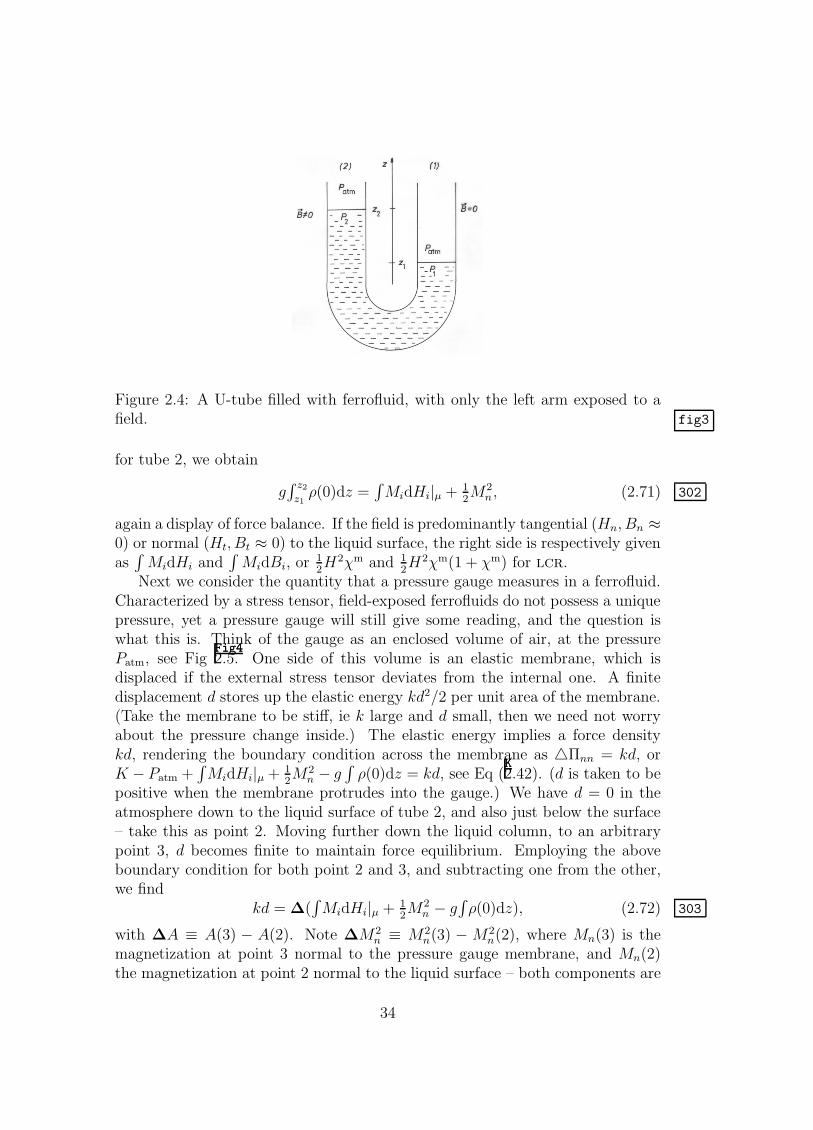
Figure 2.4: A U-tube filled with ferrofluid, with only the left arm exposed to afield. fig3
for tube 2, we obtain
g∫ z2
z1ρ(0)dz =
∫MidHi|µ + 1
2M2
n , (2.71) 302
again a display of force balance. If the field is predominantly tangential (Hn, Bn ≈0) or normal (Ht, Bt ≈ 0) to the liquid surface, the right side is respectively givenas
∫MidHi and
∫MidBi, or 1
2H2χm and 1
2H2χm(1 + χm) for lcr.
Next we consider the quantity that a pressure gauge measures in a ferrofluid.Characterized by a stress tensor, field-exposed ferrofluids do not possess a uniquepressure, yet a pressure gauge will still give some reading, and the question iswhat this is. Think of the gauge as an enclosed volume of air, at the pressurePatm, see Fig
Fig4Fig42.5. One side of this volume is an elastic membrane, which is
displaced if the external stress tensor deviates from the internal one. A finitedisplacement d stores up the elastic energy kd2/2 per unit area of the membrane.(Take the membrane to be stiff, ie k large and d small, then we need not worryabout the pressure change inside.) The elastic energy implies a force densitykd, rendering the boundary condition across the membrane as Πnn = kd, orK − Patm +
∫MidHi|µ + 1
2M2
n − g∫
ρ(0)dz = kd, see Eq (KK2.42). (d is taken to be
positive when the membrane protrudes into the gauge.) We have d = 0 in theatmosphere down to the liquid surface of tube 2, and also just below the surface– take this as point 2. Moving further down the liquid column, to an arbitrarypoint 3, d becomes finite to maintain force equilibrium. Employing the aboveboundary condition for both point 2 and 3, and subtracting one from the other,we find
kd = ∆(∫MidHi|µ + 1
2M2
n − g∫ρ(0)dz), (2.72) 303
with ∆A ≡ A(3) − A(2). Note ∆M2n ≡ M2
n(3) − M2n(2), where Mn(3) is the
magnetization at point 3 normal to the pressure gauge membrane, and Mn(2)the magnetization at point 2 normal to the liquid surface – both components are
34

Figure 2.5: A vessel filled with ferrofluid is subject to a field. The pressure insidethe ferrofluid, as measured by the membrane displacement of a pressure gauge,changes with height, orientation and the field strength.Fig4
not necessarily parallel. If the field is uniform, if the membrane of the gauge isparallel to the liquid surface, and if quasi-equilibrium holds, Eq (
3033032.72) reduce to
the zero-field hydrostatic relation, gρ(z2−z3) = kd; otherwise, field contributionsabound – even if the pressure gauge is simply rotated at point 3 in the presence ofa uniform field. (All fields are the actual ones, distorted by the gauge’s presence.)
2.5.4 Magnetic O-Rings and Scrap Separationscrap
In this section, we address the physics of some technical applications: magneticO-rings, self-levitation and scrap separation. Consider scrap separation first. Aninhomogeneous magnetic field which becomes weaker with increasing height maylift non-magnetizable bodies submerged in ferrofluids off the ground, and holdthem at specific heights which depend on the shape and density of the bodies.Balancing the gravitational and magnetic force, Fmag +Fgrav = 0, we have F grav
given by Eq (gKraftgKraft2.46), and Fmag by (
emsf3emsf32.49).
Because scrap separation is an equilibrium phenomenon, we may also considerenergy instead of force. Take first the fact that ferrofluid is attracted to regionsof higher magnetic field. If the field B is given, the field energy is B2/2 in air,and B2/(2µm) in ferrofluids. With µm > 1, the second expression is alwayssmaller. So given the choice, a volume element of ferrofluid will occupy theregion with the highest possible field. Conversely, a non-magnetizable objectsubmerged in ferrofluid will tend to occupy the region of lowest field strength.If a difference in height is involved, all these happen only as long as the gainin field energy is larger than the loss in gravitational energy. (If instead H isgiven, Fem ≡ Fem − HB is larger in vacuum then in the ferrofluid: −H2/2 >−µmH2/2.) Similarly, a permanently magnetized body submerged in ferrofluidtends to collect as much liquid in the region of its field as possible – even at theprice of levitating itself off the bottom, a phenomenon that is sometime referred
35

Figure 2.6: Self-levitation in ferrofluid of a magnetizing body. Fig5
to as “self-levitation”rz[4]. if the magnetic body consists of a periodic array of
north and south poles, with periodicity λ, the field extends one or two λ intothe ferrofluid. Levitated approximately that far from the bottom, the body willusually have reached its equilibrium position, as no further gain in field energymay be achieved levitating itself yet higher, see Fig
Fig5Fig52.6.
Magnetic O-rings may be found in most computer hard disk drives and areperhaps the most widely deployed ferrofluid device. In these, some ferrofluid ispositioned as an O-ring between a highly permeable rotating shaft and the pole ofa permanent magnet, see Fig
Fig6Fig62.7. Serving as a pressure seal, it enables the rotary
component to work in vacuum. Note that we are dealing with a metastable statehere, as it is always energetically more favorable to remove the ferrofluid sealfirst, have the pressure equalized, and then return the seal to its original placeat the poles. So the quantity of interest is the lowest energy barrier that mustbe overcome, which in any realistic problems is notoriously difficult to find. Thecorrect force balance, on the other hand, is
A∆Patm = ∆
∫(1
2M2
n +∫
MkdHk|µ)dA, (2.73) ml4
between the difference in the magnetic surface force, Eq (emsfemsf2.44), and the difference
in external pressure. [Clearly, the appropriate replacement is given by µ → µte,cf Eq (
replrepl2.28).] The field is strongest in the middle of the O-ring and decays
towards both ends. If ∆Patm were zero, the force Fmag would be the same onboth surfaces, and the ferrofluid stays in the middle of the O-ring. Increasing
36

Figure 2.7: Magnetic pressure seal: (a) principle and (b) enlarged view of theferrofluid plug. Fig6
the pressure on the left (surface 1) pushes the ferrofluid towards right, such thatsurface 1 is in the region of higher, and surface 2 is in the region of weaker,fields. Equilibrium is achieved when the difference in Fmag balances ∆Patm.The strongest pressure difference maintainable is when one surface is at the fieldmaximum and the other is field-free. Assuming for simplicity that the magneticfield is predominantly tangential, and that lcr holds, we have ∆P = 1
2χmH2.
With χm ≈ 1, H2 = µm0 H2, and taking H as of order 105A/m, this pressure
difference is about 105N/m2, approximately the atmospheric pressure.
37

Chapter 3
Dissipative Electrodynamics
geneTurning now to dynamics and off-equilibrium phenomena, we first note that thereare two types of theories: the high-resolution theory for a low density system,with at most one particle per infinitesimal volume element (or per grain, as inphotographs); and the low resolution theory for a high density system, with manyparticles per grain. The microscopic Maxwell equations and the Newtonian equa-tion of motion (including the Lorentz force) belong to the first type. There are nohidden charges, polarization or magnetization here, and we know the whereaboutsof every single particle. The second type includes the macroscopic Maxwell equa-tions, or any thermodynamic and hydrodynamic theories. The problems aboutdissipation and the coarse-grained electromagnetic force arise here.
We shall consider three systems with increasing densities, to be accountedfor by theories of decreasing resolution and growing complexities: The first sys-tem (section
highhigh3.1) is a dilute gas of charged particles, well accounted for by the
Newtonian equation of motion and the microscopic Maxwell equations. The nextsystem (section
partpart3.2) is a slightly dissociated liquid of particles possessing negligi-
ble electric and magnetic dipole moments. So there are many neutral particles,but at most one charge carrier, per grain. The appropriate theory here is ofa mixed type, a combination of the hydrodynamic theory and the microscopicMaxwell equations. The first accounts for all particles, the latter for the spatiallyslowly varying field, produced by the few charge carriers that are far apart fromeach other. Finally, in section
EoMEoM3.3, we consider a dense system possessing dipole
moments and hidden sources, which needs to be accounted for by the genuinelylow-resolution, hydrodynamic-type Maxwell theory that is our goal to derive andconsider in details. The advantage of this successive approach is, finding the morecomplicated expressions in the dense medium is rendered very much simpler andtransparent by the considerations of the previous two dilute systems – but we donot, even loosely, derive one from the other.
38

3.1 Rarefied Plasmashigh
Clearly, the microscopic Maxwell equations (m1m11.1,
m2m21.2) account for the time evo-
lution of the finely resolved fields e and b for given sources, the electric chargedensity and its current; while the feedback of the fields on the motion of thesources is given by the Newtonian equation of motion,
mαvα = qα(e + vα × b/c), (3.1) 2
one for each particle α. Eqs (m1m11.1,
m2m21.2,
223.1) represent a closed theory, frequently
rather too detailed but conceptually simple. However, it does contain a notationalinconsistency: The Maxwell equations are an Euler type theory, accounting forthe time evolution of fields at a given point in space, while the Newtonian equationis of the Lagrange type, which concentrates on a given particle. (So the termje = ρev in Eq (
m2m21.2) denotes the electric current at a space point, while vα in
Eq (223.1) is the velocity of particle α.) As only the Euler formulation lends itself
to a reduction of the resolution, we shall first find the Euler version of Eq (223.1),
with a resolution high enough that each grain contains at most one particle. (Thistheory is meant as a starting point, to clarify a few concepts important for themore complex theories of the following chapters. So we shall simply discard thepossibility that even in a rarefied gas, two particles will occasionally come closeto each other.)
3.1.1 The Eulerian Newtonian Equationeule
Taking the volume of the grain as VG, we may identify its velocity, mass andcharge with that of the particle occupying it at a given instance, and takeall three to be zero if there is no particle: vα → v(r, t), mα/VG → ρ(r, t),qα/VG → ρe(r, t), defining three highly discontinuous fields. The many Newto-nian equations of motion then reduce to one field equation,
ρ ddt
v ≡ ρ[v + (v · ∇)v] = ρe(e + v × b/c). (3.2) 3
(The quantity ∇v is taken from the velocity of the same particle at two successivemoments.) It is now essential to include the continuity equation,
ρ + ∇ · (ρv) = 0, (3.3) 4
which in the Lagrange version is implicit, nearly incidentally contained in thefact that one does not loose any of the many equations (
223.1). The energy and
momentum density are respectively,
uM = ρ(c2 + v2/2), gM = ρv, (3.4) 5
39

where the energy comprises of the rest energy and the (non-relativistic) kineticenergy. Employing Eqs (
333.2,
443.3), we find
uM + ∇ · QM = je · e, (3.5) 7
gMi + ∇k ΠM
ik = (ρee + je × b/c)i, (3.6) 8
QM = uMv, ΠMik = gM
i vk. (3.7) 9
3.1.2 The Field Contributionsfiel
The field contribution to the energy and momentum density are
uF = 12(e2 + b2), gF = e × b/c. (3.8) 11
From the Maxwell equations (m1m11.1,
m2m21.2) we deduce
uF + ∇ · QF = −je · e, QF = c e × b, (3.9) 12
gFi + ∇kΠ
Fik = −(ρee + je × b/c)i, (3.10) 13
ΠFik = (e2 + b2 − uF)δik − eiek − bibk. (3.11) 15
Note the relationship gF = QF/c2. This is far from accidental and derives fromthe symmetry of the relativistic energy-momentum 4-tensor, ΠF
αβ = ΠFβα, because
cgFk = ΠF
k4, QFk/c = ΠF
4k. Less formally, gF = QF/c2 may also be seen as fieldangular momentum conservation for ρe → 0. The angular momentum densityF ≡ r×gF is a locally conserved quantity in neutral systems. Rewriting Eq (
13133.10)
(with ρe → 0) as ∂Fi /∂t+∇m(εijkrjΠ
Fkm) = εijkΠ
Fkj , we observe that the angular
momentum Fi satisfies a continuity equation only if the stress tensor is symmetric.
Although this argument seems to require merely the symmetry of the momentum3-tensor, ΠF
ik = ΠFki, a nonvanishing ΠF
k4 −ΠF4k in one inertial system will foul up
the symmetry of the 3-tensor in other systems, as the antisymmetric parts of any4-tensors mix in a Lorentz transformation. Yet angular momentum is conservedin every inertial system.
Since this reasoning is so general, it also holds for the material part, gM =QM/c2. Hence the expression for the momentum density is in fact gM = ρv[1 +v2/(2c2)], cf Eqs (
553.4,
993.7) – though we are quite justified to neglect the second
term in the nonrelativistic limit. Later, when we have no prior knowledge of theform of the momentum density, we shall deduce it from that of the energy flux,as angular momentum is also conserved in dense systems.
We register the fact that while the expression for the energy density uF =12(e2 + b2) is a genuine input – independent of and in addition to, the Maxwell
equations, the formula gF = e × b/c is not, since QF is given once uF is. More-over, since Eq (
13133.10) then follows from the Maxwell equations, and because total
momentum is conserved (see sectionconscons3.1.3), the Lorentz force is a result as well.
40

3.1.3 Energy and Momentum Conservationcons
The preceding two sections allow the simple and noteworthy conclusion thatour starting equations imply local conservation of total energy, momentum andangular momentum in the presence of charge, ρe = 0. Taking u ≡ uF + uM andg ≡ gF + gM , we find
u + ∇ · Q = 0, gi + ∇kΠik = 0, (3.12) 16
Πik = Πki = ΠFik + ΠM
ik , Q = QF + QM , (3.13) 20
Q/c2 = g ≈ ρv + e × b/c. (3.14) 18a
These results have been collected here because local conservation of these quan-tities is always true, independent of the above derivation tailored to a dilute andfinely resolved system. So we may use them as input next.
3.2 Weakly Dissociated Liquidspart
Now we consider a dense macroscopic system in its hydrodynamic regime: Tothe above gas of dilute charge carriers we add a dense system of neutral particleswith vanishing electric and magnetic dipole moments. This is still a compara-tively simple system, as the highly resolving, vacuum Maxwell equations (
m1m11.1,
m2m21.2)
remain valid – and with them all the equations about field energy and momentumin
fielfiel3.1.2. The equations in
euleeule3.1.1, concerning the respective material contributions,
must be modified, as these are now accounted for by three smooth and slowlyvarying hydrodynamic variables: the coarse-grained densities of mass, energy andmomentum 〈ρ〉, 〈uM〉, 〈gM〉, taking the entropy density s as a function of them.(The coarse-graining brackets are dropped below to keep the notation simple.)
3.2.1 The Material Contributionsmate
We first consider the hydrodynamic theory of a neutral, isotropic liquid. Itconsists of continuity equations for the densities of mass, energy, momentum:ρ, uM , gM , and a balance equation for the entropy s, with a source term RD/T ,
ρ + ∇·j = 0, s + ∇·f = RD/T, (3.15) 26-1
uM + ∇·QM = 0, gMi + ∇k ΠM
ik = 0. (3.16) 27-1
The fluxes j, f , QM , ΠMik and the entropy production RD are not yet specified
and need to be determined. As we retrace how they are derivedLL6[16], we learn to
use the same method to set up the equations for our third system, to derive thehydrodynamic Maxwell theory.
The present theory is in two points fundamentally different from the previousone. First, dissipative terms appear in the equations of motion, breaking their
41

time-reversal symmetry. These will be marked by a superscript D. Second isour ignorance of the explicit form of uM , the material energy. Nevertheless,gM = ρv remains an excellent approximation, because the energy flux QM isstill dominated by the term c2ρv, accounting for the transport of rest energy, cfEqs (
553.4,
993.7). In nonrelativistic physics, it is not customary to include the rest
energy in uM . This represents a shift to a different set of conserved quantities:from uM , ρ to uM = uM−ρc2, ρ, implying Q
M= QM−c2ρv. This changes the link
between the momentum density and the energy flux to gM = QM
/c2 + ρv ≈ ρv.We follow this convention, but drop the bar, from here on.
To compensate for our ignorance of uM , we resort to thermodynamics. As-suming that the energy is a function of s and ρ in the rest frame of the liquid(denoted by the subscript 0), we write
duM0 =
∂uM0
∂sds +
∂uM0
∂ρdρ ≡ Tds + µ0dρ. (3.17) 21
In a liquid with a finite velocity v, we have uM = uM0 + (gM)2/2ρ. Because
d[(gM)2/2ρ] = v · dgM − 12v2dρ, Eq (
21213.17) is generalized to
duM = Tds + µdρ + v · dgM , (3.18) 23
where µ = µ0 − 12v2 is the lab-frame chemical potential.
Taking the time derivative of Eq (23233.18), uM = T s +µρ + v · gM , we have
a relation which Eqs (26-126-13.15,
27-127-13.16) must identically satisfy – irrespective how uM
(and T, µ, v) depend on s, ρ, gM . This is therefore a strong constraint, enoughto unambiguously determine all the fluxes. (This approach is sometimes referredto as the “standard procedure,” see
dGM,LL6,henjes[7, 16, 17]. It was first applied to electro-
magnetism inhymax[18] to derive the dissipative terms.) An necessary and remarkable
result is that the fluxes are given in terms only of the variables and the conjugatevariables appearing in Eq (
23233.18). Without an explicit expression for uM , the
equations clearly must be written in these general quantities, and we may takethis observation as an indication that hydrodynamic theories contain only con-servation laws and thermodynamics as input – the reason for its general validity.
Defined as the energy change if the volume changes at constant entropy andmass, the pressure P is related to the variables and conjugate variables of uM viathe Duhem-Gibbs (or Euler) relation, cf
druckdruck2.4,
P ≡ −∂(∫
uM0 d3r)/∂V = −uM
0 + Ts + µ0ρ
= −uM + Ts + µρ + v · gM . (3.19) 31
Specifying that one term in the momentum flux of Eq (27-127-13.16) is the pressure,
ΠMij = Pδij + πij (there is no loss of generality, as πij must now be determined),
we combine Eqs (23233.18,
31313.19) to obtain ∇P = s∇T + ρ∇µ + gM
k ∇vk, and write
42

uM = T s + µρ + v · gM as
∇·QM = ∇i(µji + Tfi + vkπik) − (ji − ρvi)∇iµ (3.20) standard1
−RD − (fi − svi)∇iT − (πik − vkgi)vik,
where vik ≡ 12(∇ivk+∇kvi). Postponing the question of uniqueness for a moment,
we identify QMi = µji + Tfi + vkπik, set fD
i ≡ svi − fi, ΠDik ≡ vkgi − πik, and
ji − ρvi = 0, to obtain RD = fDi ∇iT + ΠD
ikvik. (The dissipative mass current,jDi ≡ ji−ρvi, is a relativistically small quantity that we shall neglect, see
3cd[19] and
the footnote in sectionhydrhydr3.2.3.) Identifying fD
i , ΠDik as the dissipative fluxes, ∇iT ,
vik as the thermodynamic forces, we follow the Onsager prescription to take themas pairwise proportional
LL5[20], yielding heat conduction and the viscous stress,
fDi = κ∇T, ΠD
ik = ηvik + ζδikvnn. (3.21) onsager1
Clearly, all fluxes have now been determined, especially fi = svi − fDi and ΠM
ik =Pδik + vkgi −ΠD
ik. Without dissipative terms, the energy and momentum flux areQM
i = (uM +P )vi, ΠMik = gM
i vk +Pδik, and the only difference to Eqs (993.7) is the
pressure P , an indication for a dense and interacting system.The question remains whether the conclusion we draw from Eq (
standard1standard13.20) is
unique. The answer is yes, because all terms must be written such that theycan be assigned to one of two groups. Either it is the divergence of something,then it belongs to the energy flux QM ; or it vanishes in equilibrium, like ∇iT , vij ,then it is part of RD. For instance, the term T s = −T∇ifi + · · · must be writtenas fi∇iT − ∇i(Tfi), with the first term contributing to RD, and the second toQM . All terms in Eq (
standard1standard13.20) clearly belong to one of the two groups, and there is
no possibility to change them such that this feature is maintained.
3.2.2 The Field Contributionsmate2
Next, we consider finite electric charges and currents. Collecting all terms derivedabove, and adding the ones that become finite with ρe, je, we have
ρ + ∇·(ρv) = 0, s + ∇·(sv − fD) = RD/T, (3.22) 26
uM + ∇i[(uM + P )vi − TfD
i − vkΠDik] = je · e, (3.23) 27
gMi + ∇k (Pδik + gM
i vk − ΠDik) = (ρee + je × b/c)i, (3.24) 28
RD = fDi ∇iT + ΠD
ikvik + (je − ρev) · e0. (3.25) add2
The right sides of Eqs (27273.23,
28283.24) have the given form because the source terms
of Eqs (12123.9,
13133.10) remain unchanged, and summing up the respective right sides
must yield nil, as in Eqs (16163.12), such that total energy and momentum remain
conserved. The third term in RD goes beyond the sum of microscopic Maxwellequations and the hydrodynamics of neutral fluids, it needs to be derived. The
43
point is, je is no longer given by ρev as in sectionfielfiel3.1.2, because v is now the ve-
locity of a volume element containing many particles. Given a finite electric field,e0 = e+v×b/c, in the rest frame of the volume element, electric charge carrierswill move with respect to this volume. This is exactly what we obtain startingfrom Eq (
add2add23.25), identifying je − ρev as the current, e0 as the thermodynamic
force, and following Onsager to take them proportional,
(je − ρev)i ≡ (jDe )i = σij(e + v × b/c)j, (3.26) onsager2
where σij = σ‖bibj + σ⊥(δij − bibj) + σHεijkbk, with σ‖, σ⊥ being the conductivityalong and perpendicular to b, and σH accounting for the Hall effect. (A thermo-electric term α∇T is sometimes relevant, together with αe0 in fD.)
Now we derive the third term in RD, Eq (add2add23.25), by again taking the temporal
derivative of Eq (23233.18), uM = T s+µρ+v · gM . Dropping terms not containing e
or b, we find ∇iQMi = −RD +e ·je−v ·(ρee+je×b/c) · · · , where the second term
is from uM , and the third from gM . Combing them as −je(e− b× v/c) +e · ρev= −(je−ρev)e0, because e·v = e0 ·v, we obtain ∇iQ
Mi = −RD · · ·+(je−ρev)e0.
Because e0 = 0 in equilibrium, the last term is part of RD, concluding the proof.Inserting ∇P = s∇T + ρ∇µ + gM
j ∇vj and the first of Eq (26263.22) into (
28283.24),
we obtain an equation that will prove useful for later comparison,
ρ ddt
vi + s∇iT + ρ∇iµ + gMk ∇ivk (3.27) 31a
= ∇kΠDik + (ρee + je × b/c)i.
Adding the Maxwell equations (m1m11.1,
m2m21.2), the system of equation is closed and
the description complete. With ρe given by ∇ ·e, and uM by Eq (23233.18), the inde-
pendent variables are ρ, s, gM , e, b. Referred to as the magneto-hydrodynamics,these are realistic equations, used for describing plasmas at low frequencies
LL8[2].
Usually, σ‖, σ⊥ are large, hence ρe, e0 = e + v × b/c negligibly small.
3.2.3 The 2-field Theoryhydr
In the low-resolution theory of the next chapter, we shall be dealing with densesystems containing hidden charges and dipole moments. The obvious consequenceis the appearance of four fields (E, D, B, H) – replacing (e, b) here. An equallyimportant difference is the fact that (the possibility of an expansion notwith-standing) we no longer have an expression for the field energy uF – which wasimportant for arriving at the right-side terms of Eqs (
27273.23,
28283.24), especially the
Lorentz force. In fact, it will not even be possible to separate the total, con-served energy density u into uF and uM , such that the former depends on thefield variables alone, and the latter on the material ones. In the simple exampleu = u(ρ, s) + 1
2B2/µm(ρ, s), the temperature T = ∂u/∂s + 1
2B2∂(1/µm)/∂s is a
function of B, and H = B/µm depends on s. As a result, none of the variablesor conjugate variables is unambiguously assigned to either field or material 1.
44

Fortunately, neither the Lorentz force nor a division of u and g into materialand field contributions are necessary for deriving the hydrodynamic Maxwelltheory. As a first step, we shall convince ourselves that the present theory canbe equally well written in the variables u ≡ uF + uM , g ≡ gF + gM , such thatthe Lorentz force never appears. We do this by adding up the material and fieldcontributions of
fielfiel3.1.2 and
matemate3.2.1 (as in section
conscons3.1.3), obtaining
u + ∇i(QRi − QD
i ) = 0, (3.28) 27A
gi + ∇k (ΠRik − ΠD
ik) = 0, (3.29) 28A
QR ≡ (Ts + µρ + v · gM)v + c e × b, (3.30) 36
ΠRik ≡ gM
i vk − eiek − bibk + δik ×(Ts + µρ + v · gM − u + e2 + b2). (3.31) 37
g = gM + e × b/c = ρv + QR/c2. (3.32) gm
The dissipative terms, ΠDik and QD
i ≡ TfDi + vkΠ
Dik, remain as given above. Note
QD does not contribute to the total momentum density,2 see Eq (gmgm3.32). The
expression for du is obtained by adding the first of Eqs (11113.8) to Eq (
23233.18),
du = Tds + µdρ + v · dgM + e · de + b · db (3.33) 32
= Tds + µdρ + v · dg + e0 · de + b0 · db. (3.34) 33
Eq (33333.34) is algebraically identical to Eq (
32323.33), because v · d(gM − g)c = −v ·
d(e×b) = −(v×e) ·db+(v×b) ·de, where e0 ≡ e+(v/c)×b, b0 ≡ b−(v/c)×eare the respective rest frame fields.
Containing ρ, s, u, g, e, b as variables, the new theory is given by the Maxwellequations (
m1m11.1,
m2m21.2), the equations for mass and entropy (
26263.22), and all the dis-
played equations of this section. It is closed, complete and quite equivalent to theold one. We may refer to it as the “2-field” theory, and require that the genuinelylow-resolution “ 4-field” theory reduces to it by setting ED, HD = 0, and
E = D → e, H = B → b, (3.35) 2to4
implying also E0 = D0 → e0, H0 = B0 → b0.
1This is the reason why attempts, by people including Minkowski, to divide the total, con-served momentum density g into gM and gF is such a futile exercise, see discussion in
henjes[17].
2This is a subtle point. The quick argument is, as a variable, g must not contain termsof different time-inversion parity. The more complete argument is, the existence of a finiteQD is in fact the result of subtracting the rest energy from the total – without which thedissipative energy flux vanishes identically. As shown in
3cd[19], there is a connection between
this and the vanishing of the dissipative mass current, jD: Taking the mass, energy and totalenergy conservation as ρ + ∇i(ρvi + jD) = 0, u + ∇i(Qi − QD
i ) = 0, utot + ∇iQi = 0, wehave utot = u + ρc2 and Qi = Qi + ρvic
2 = gic2, with QD
i = 0, or jDi c2 − QD
i = 0. BecausejDi = QD
i /c2 is a relativistically small quantity, it is usually neglected.
45

3.2.4 Radiation Damping
Let us briefly address the old problem of radiation damping, which has createdconsiderable confusion in some textbooks, with the result that a good number ofphysicists take it to be an indication for the inconsistency of the Maxwell theory.The basic physics of radiation damping is in fact given by the equations derivedin
hydrhydr3.2.3, stating conservation of total energy and momentum. So it is an easy
conclusion to draw that if a charged body’s acceleration generates radiation, itwill lack exactly the energy and momentum that is being carried away by theradiation. This is all we need to know about radiation damping, and there is noreason whatever why it is not consistently accounted for by the above equations.
The problems such as discussed injackson[1] arise from two sources: First and fore-
most, it is the usual yet unreasonable insistence to reduce the above derived setof differential equations of
hydrhydr3.2.3, the 2-field theory, to a term or two, ∼ v, v, in the
Newtonian equation of motion for the charged body. Failure of this oversimplifieddescription is not connected to any inconsistencies of the Maxwell theory. Sec-ond, and less centrally, it also stems from the fruitless attempt to describe pointcharges employing the Maxwell theory – constructed to account for finite chargedensities. Although electrons may well be infinitely small, one can at most criti-cize the Maxwell theory for not being realistic (in this extreme quantum limit),but not for being inconsistent.
3.3 The Hydrodynamic Maxwell TheoryEoM
The low-resolution, hydrodynamic theory we are going to consider is fairly gen-eral, valid for arbitrarily strong fields and nonlinear constitutive relations, withthe medium moving and the electromagnetic field time-dependent. (Relativisticterms are not included here. The fully covariant form of these equations maybe found in
rel[21].) However, it is a local-equilibrium theory with a confined fre-
quencies range. To go beyond it, additional, nonhydrodynamic variables such asmagnetization and polarization need to be included, see section
outlookoutlook3.5.
3.3.1 Frame-Independent Thermodynamics
The conserved density of total energy u, of a moving, one-component liquid is afunction of s, ρ, D, B, and in contrast to Eq (
22221.12), also of the conserved total
momentum density g. We therefore write
du = Tds + µdρ + v · dg + E0 · dD + H0 · dB, (3.36) 40
with the conjugate variables given as always by differentiating the energy withrespect to the variable. E0, H0 are necessarily rest frame fields, as we know from
46

Eqs (33333.34,
2to42to43.35). The associated equilibrium conditions are
∇ × H0 = 0, ∇ × E0 = 0 (or E0 = 0), (3.37) ec2
∇T = 0, vij = 0, v + ∇µ = 0. (3.38) ec3
The three equations of the first line are deduced starting from Eq (40403.36), going
through the same steps as those leading to Eqs (smesme1.14). Clearly, in spite of the
more general starting point, these conditions have not changed. They are stillgiven by setting, in the local rest frame, either the curl or the field itself to zero,nicely illustrating that the fact of being in equilibrium does not depend on theframe of reference. ∇T = 0 is also unchanged, and the last two equations areobtained by keeping momentum, angular momentum and the booster constant.The details are in
3cd[19], and not reproduced here, because it is off the present focus
on the Maxwell theory. Vanishing vij allows only motions that are combinationsof translation and solid-body rotation. Not being Galilean invariant, the chemicalpotential µ has additional terms when the system rotates and translates. Thegradient of these terms is canceled by v.
For the microscopic theory of sectionhighhigh3.1, or the partially microscopic one
ofpartpart3.2, with the material and field variables clearly separated, the inconsistency
of employing the Galilean transformation for one type of variables, and Lorentztransformation for the other, is not of too much concern. This is different now. Wecan of course always construct a fully covariant theory, or for small velocities, onethat is covariant to linear order in v/c. Both are possible and have been done
rel[21],
with unnecessarily complicated formulas, as there is, in usual laboratory physics,simply no need to include terms distinguishing the rest-frame spatial derivative∇0 from that of a moving one, ∇ = ∇0 − 1
c2v∂t, if ∇ is to operate on a material
variable. Yet this difference, when ∇ operates on a field variable, is relevantfor maintaining the form-invariance of the Maxwell equations. Unfortunately,due to the interdependence of variables, say ∇µ = [∂µ/∂ρ]∇ρ + [∂µ/∂H ]∇H +· · · , the difference between both is quite ambiguous. Facing this dilemma, apractical solution is to postulate a Galilean invariant ∇, find the appropriatefield transformation that will leave the Maxwell equations invariant, and finallyverifying that the terms being left out are not important.
First, given the fact that the charge density ρε = ∇ · D, similar to the massdensity, is (to linear order in v/c) a scalar, D must also be one. Taking ∇ · Bto be a scaler too, so is B. In equilibrium and for a medium at rest, becauseboth B = −c∇ × EM and ∇ × E0 vanish, we deduced in section
EmstaEmsta1.3 that
B = −c∇ × E0; and similarly D = c∇ × H0. For a translating and rotatingmedium in equilibrium, D and B move with the medium, such that each materialpoint keeps their values, and the temporal derivatives in the local rest frame, dtDand dtB vanish. They relate to the laboratory quantities as
dtD ≡ D + (v · ∇)D − Ω×D = 0, (3.39) dt1
dtB ≡ B + (v · ∇)B −Ω×B = 0, (3.40) dt2
47
where Ω ≡ 12(∇ × v). So the properly generalized equations are
dtD = c∇ × H0, dtB = −c∇ × E0. (3.41) dt4
On the other hand, because of locality and charge conservation, we know thatthe Maxwell equations always have the structure
B = −c∇ × EM , D + jε = c∇ × HM . (3.42) dt3
Defining E = EM , H = HM to be the Maxwell fields of an arbitrary inertialframe in equilibrium, we find that Eqs (
dt3dt33.42) and (
dt4dt43.41) are equivalent (neglecting
terms ∼ vij as it vanishes in equilibrium), with the identifications jε = ρεv, and
E ≡ E0 − (v/c) × B, H ≡ H0 + (v/c) × D. (3.43) gal-trans
The microscopic fields e, b form a tensor and mix in a Lorentz transformation,as e = e0 −v×b0/c, b = b0 +v×e0/c to linear order. We may therefore deducethat E, B form a tensor, and D, H another, mixing respectively with each otherin a boost. (Off equilibrium, B forms a tensor with EM , and D with HM .) Thisis indeed true in a covariant theory, appropriate if v/c is not negligible. In our“effective Galilean” theory, we retain only terms not diminished by the factor v/c.Hence ∇ = ∇0 −v∂t/c
2 is taken as invariant, but not ∂0t = ∂t +v ·∇. Similarly,
we omit the second term in B = B0+(v/c)×E, but retain the corresponding oneon the right side of the Maxwell equation, −c∇×E = −c∇×E0−∇× (v×B).If for any reason the first term −c∇ × E0 is small — the local electric field E0
vanishes in a conductor in equilibrium — the normal-size second term is quiterelevant, as we shall see in section
oee1oee13.4.1.
In a satellite containing a superconducting coil and a magnetizable medium,the field is in general non-uniform. Yet if coil and medium co-rotate and co-translate, dtD, dtB = 0, the system may stay in equilibrium, ∇×E0, ∇×H0 = 0,maintaining its motion for ever, with given total momentum and angular momen-tum. On earth, the magnetic coil is usually fixed, and the field stationary in thelab-frame. If the medium rotates, with Ω×B = 0, all four quantities, dtD, dtB,∇ × E0, ∇ × H0 are finite, the motion is dissipative and will eventually stop.The examples of section
oee2oee23.4.2 and
fevfev3.4.3 concern this effect about the temporal
term ∼ Ω in Eq (dt2dt23.40). However, because Eqs (
dt4dt43.41) and (
dt3dt33.42) are equivalent,
it is in fact indistinguishable from the transforming field terms of Eqs (gal-transgal-trans3.43).
With Eqs (gal-transgal-trans3.43), we may write the energy, Eq (
40403.36), as
du = Tds + µdρ + v ·dgM + E ·dD + H ·dB, (3.44) 42
gM ≡ g − D × B/c, (3.45) 43
generalizing Eq (32323.33). Note Eq (
43433.45) is only a shorthand, the result of going
from Eq (40403.36) to (
42423.44). As we shall see, in all the fluxes of the hydrodynamic
48

equations, this gM will replace the material momentum density gM = ρv ofsection
matemate3.2.1. But there is no further implication, especially not that this gM
were the unambiguous material part of the momentum density here.Note that although we take the two pairs of fields to transform differently,
their basic functional dependence does not change. We have E0, H0 as functionsof D, B (with E0 = D/ε, H = B/µm linearly), and E, H given by Eq (
gal-transgal-trans3.43).
In their classic book, De Groot and Mazur devoted a chapter to consideringthe same physics, aiming to set up a theory to account for the hydrodynamicsof polarizable and magnetizable systems. Unfortunately, they started from thesuperficially plausible thermodynamic relation, du = · · ·+v·dg+E·dD+H·dB,overseeing the crucial difference between g and gM . Worse, they ruled out thepossibility of dissipative fields, setting HD, ED to zero.
3.3.2 Reactive Terms
The complete set of equations of motion, valid also off equilibrium, is
D = c∇ × HM− jε, B = −c∇ × EM, (3.46) M5
ρ + ∇ · (ρv) = 0, s + ∇ · f = RD/T, (3.47) 26x
u + ∇ · Q = 0, gi + ∇k Πik = 0. (3.48) 16xx
It simply states that conserved quantities satisfy continuity equations, and fieldvariables the Maxwell equations – expressing locality and charge conservation.To obtain the fluxes, HM , EM , f , Q, Πik, and the entropy production RD, weproceed as in
matemate3.2.1 and
mate2mate23.2.2, by inserting the equations of motion into the tem-
poral derivative of Eq (40403.36), u = T s + µρ + v · g + E0 · D + H0 · B, and sorting
the terms to be either part of a divergence, or proportional to a thermodynamicforce that vanishes in equilibrium. The result is ∇ ·Q = ∇ ·Q1 +RD−R1, where
R1 ≡ (jε − ρεv) · E0 − (fi − svi)∇iT − (Πik − ΠRik)vik (3.49) RD
+(EM − E) · c∇ × H0 − (HM − H) · c∇ × E0,
Q1i ≡ Tfi + (µρ + v · gM)v + (Πik − ΠR
ik)vk +
c[E×H + (EM − E)×H0 + E0×(HM − H)]i. (3.50) 39
ΠRik ≡ gM
i vk − EiDk − HiBk + δik×(Ts + µρ + v · gM − u + E · D + H · B), (3.51) 146
Concluding Q = Q1 and RD = R1, we take all the flux-force pairs to be pro-portional to each other. In equilibrium, the forces vanish, ∇T , vik, c(∇ × H0),c(∇ × E0), E0=0, and hence we have: f = sv, Πik = ΠR
ik, jε = ρεv, EM = E,HM = H , and especially
Q = (Ts + µρ + v · gM)v + c E × H . (3.52) 146qr
49

These expressions correctly reduce to the 2-field theory, especially Eqs (36363.30,
37373.31). Also, for v = 0, the stress ΠR
ik reduces to that of Eq (51x51x2.7).
Consider the rotational invariance of the energy u to see ΠRik = ΠR
ki is symmet-ric: Rotating the system by an infinitesimal angle dθ, the scalars are invariant,du, ds, dρ = 0, while the vectors change as dgM = gM × dθ, dD = D × dθ,dB = B × dθ. Inserting these into Eq (
42423.44) yields,
εijkΠkj = (v × gM + E × D + H × B)i = 0. (3.53) 64
For vanishing fluid velocity and linear constitutive relations, v ≡ 0, εE = D andµmH = B, the symmetry of the stress tensor is obvious, otherwise it is not.
3.3.3 Dissipative TermsOnsager
With dissipation, RD = 0, the above expressions for the fluxes are amended bydissipative contributions,
f = sv − fD, Πik = ΠRik − ΠD
ik, jε = ρεv + jDε , (3.54) fd2
EM = E + ED, HM = H + HD, (3.55) hd2
Assuming a diagonal Onsager matrix, we obtain Eqs (onsager1onsager13.21,
onsager2onsager23.26), and
ED = βc∇ × H0, HD = −αc∇ × E0, (3.56) dis1
the generalization of Eqs (edhd2edhd21.19). Unfortunately, the Onsager matrix tends not to
be diagonal, with typically longish off-diagonal elements. An elegant alternativeto dealing with them directly is to rewrite the entropy production R as a sum ofdifferent force-flux pairs, looking for one the diagonal form of which is a betterapproximation. For instance, given the entropy production, R = aA+bB, insteadof writing cross terms, a = αA + γB, b = βB + γA, we may take R as R =aA + bB − γ
α(Ba−Ba) = (A + γ
αB)a +B(b− γ
αa), and assume a Onsager matrix
diagonal in the new force-flux pairs, a = α(A + γαB), b − γ
αa = (β − γ2
α)B. Both
sets of equations of motion are obviously the same.The rest-frame derivatives, dtBi and dtDi, may be written as
dtBi = −c(∇× [E0 + ED])i − Bivkk + Bkvik, (3.57) ec5
dtDi = (c∇× [H0 + HD] − jD)i − Divkk + Dkvik,
employing Eqs (gal-transgal-trans3.43,
M5M53.46). Being linear combinations of quantities that vanish
in equilibrium, they are legitimate, alternative thermodynamic forces. Rewritingthe entropy production in terms of these forces, we find ∇·Q = ∇·Q1+RD−R1 =
50

∇ ·Q2 + RD −R2, with Q2 = Q1 + ED ×HD, R2 = R1 + ∇ · (ED ×HD), and
R2 ≡ fD ·∇T + ΠDikvik + HD ·dtB + ED ·dtD + jD · EM
0 , (3.58) ver2RD
Q2i ≡ Tfi + (µρ + v · gM)vi − ΠD
ikvk + c[EM×HM ]i (3.59) ver2Q
+12(BiH
Dk − BkH
Di + DiE
Dk − DkE
Di )vk
Πik ≡ ΠRik − ΠD
ik + (BjHDj + DjE
Dj )δik (3.60) ver2pi
−12(BkH
Di + BiH
Dk + DkE
Di + DiE
Dk ).
Identifying Q = Q2, RD = R2, and assuming a diagonal matrix, we have
HD = αdtB, ED = βdtD, jD = σEM0 , (3.61) hd
fD = κ∇T, ΠDik = ηvik + ζvllδik, (3.62) pd
where α, β, σ, κ, η, ζ are transport coefficients – different from those of Eqs (onsager1onsager13.21,
dis1dis13.56). [More generally, these are matrices, as in Eq (
onsager2onsager23.26).] Insert the expres-
sions into Eq (hd2hd23.55), to find EM , HM ; into Eq (
ver2piver2pi3.60) to find the stress Πik; into
Eq (fd2fd23.54) to find the entropy flux f and electric current jε. Though off-diagonal
terms are needed for a complete account, these fluxes are frequently a good ap-proximation, eg for ferrofluids exposed to weak fields, see section
oeeoee3.4, and
mdot[22].
Finally, note that although the above manipulation consists mainly of rewrit-ing RD to find a different set of force-flux pairs, the energy flux and the entropyproduction were also slightly altered, by the term ∇ · (ED ×HD), rendering thetwo sets of expressions, if both ED and HD are finite, inequivalent. (This termis both the divergence of something, and vanishes in equilibrium, it can thereforebe part of either the energy flux Q or the entropy production RD, a rare instanceof inconclusiveness of the standard procedure.) The discussion of the four exper-iments in section
oeeoee3.4 remain valid for either cases, but the so-called sq-modes,
considered insqmax[23] and relevant for systems, in which both the magnetic and elec-
tric dissipation are sufficiently large, where neither α nor β may be neglected,are modified for Q2, R2.
3.3.4 Relevance of the Results
For stationary media, v ≡ 0, the energy flux is Q2 = cEM × HM − TfD,demonstrating the validity of the Poynting theorem in the presence of dissipation.For a moving medium, there are additional terms, the second line of Eq (
ver2Qver2Q3.59),
that depend on the field, invalidating the Poynting theorem. The Maxwell stressΠik of Eq (
ver2piver2pi3.60) may be written as
Πik = ΠRik(H → HM , E → EM) − ΠD
ik (3.63) pi-alt
+12(BkH
Di − BiH
Dk + DkE
Di − DiE
Dk )
= 12[ΠR
ik(HM , EM) + (i ↔ k)] − ΠD
ik,
51

[if one substitutes HM , EM for H , E in ΠRik of Eq (
1461463.51)]. It is of interests in this
context to revisit the discussion in §80, 81 ofLL8[2], in which the authors lamented
the ignorance about the form of the Maxwell stress in the presence of dissipation.It is instructive to retrace the considerations of section
forceforce2.2, to obtain the off-
equilibrium expression for the bulk force density, the generalization of Eq (56562.19)
and (31a31a3.27). Inserting gM
i +∇k(gMi vk) = ρ d
dtgM
i /ρ and ∂∂t
(D×B)i/c = ∇k(BkHMi +
DkEMi )−Bk∇iH
Mk −Dk∇iE
Mk −ρεE
Mi −(jε×B)i/c into momentum conservation,
gi + ∇k Πik = 0, using the stress of Eq (pi-altpi-alt3.63), we find
ρ ddt
(gMi /ρ) + s∇iT + ρα∇iµα + gM
k ∇ivk −∇kΠDik
= (ρεEM + jε × B/c)i − HD
k ∇iBk − EDk ∇iDk
+12[∇ × (B × HD + D × ED)]i, (3.64) 56...
where ΠDik, H
Dk , ED
k are given by Eqs (hdhd3.61,
pdpd3.62). Clearly, the original bulk force
remains s∇iT +ρα∇iµα+gMk ∇ivk, though the Lorentz force is now given in terms
of EM . Two more dissipative forces ∼ ED, HD are now operative, one longitu-dinal and the other transversal. For the magnetic case, the first is HD
k ∇iBk =αdtBk∇iBk, finite if dtB‖B; while the second, 1
2∇ × (B × HD), is finite if
dtB ⊥ B – which is the case eg. when the field rotates while the medium isstationary, or more usually, when the the medium rotates in the presence of astationary field, B = 0, Ω = 0. If B‖H , [valid only for v = 0 and if H(B)does not depend on the electric field,] one can write this force as 1
2∇× (B×M ),
because B × HD = B × HM ≡ B × (B − M) = −B × M .The force 1
2∇ × (B × M) is used to account for the dissipative behavior
of ferrofluids, seerz[4], and widely believed to be connected to ferrofluids being
suspensions, as it is derived from the internal angular momentum of the parti-cles
mdot1[6]. Yet as we now realize, it is the transversal part of dissipative force, and
quite generic. There is no reason whatever it should not exist in homogeneoussystems, fluid or solid.
We consider the magnetization M to estimate the size of the coefficient α. Inequilibrium and assuming lcr, Meq = χB = (1 − 1/µm)B. Off equilibrium, itrelaxes, M = −(M − Meq)/τM , implying (1 − iωτM)M = χB in Fourier-space.Confining our consideration to small frequencies, we have M = (1+ iωτM)χB, orM = Meq − τMχB. Inserting this into HM = B − M = B − Meq + τMχB, andidentifying B − Meq as H , we find α = τMχ, or
α = τM (1 − 1/µm), β = τP (1 − 1/ε). (3.65) tau
The second equation is given by an analogous consideration of the polarization.To generalize the boundary conditions discussed in
surfFsurfF2.3.2, we note that the
connecting conditions for fields are now Dn,Bn, EMt ,HM
t = 0. As aresult, especially the condition Πtn = 0 is no longer automatically satisfied andhence contains useful information. At a free surfaces contiguous to atmosphere,
52

employ Eq (pi-altpi-alt3.63) with vn = 0 at the surface to see it reducing to
BnHDt − BtH
Dn + DnED
t − DtEDn = 1
2η(∇nvt + ∇tvn). (3.66) gbc1
We shall use this boundary condition to consider the shear force exerted by arotating field on the surface of a magnetizable liquid.
3.3.5 The Total Momentum Densitytmd
All expressions of this section,EoMEoM3.3, are valid irrespective of the explicit form of
the total, conserved momentum density g, whether it is given by ρv + E ×H/c,or ρv+D×B/c – to pick two historically popular forms, forwarded among othersby Einstein, Minkowski and Abraham
henjes[17]. Yet the rigorous identity, g = Q/c2
discussed ineuleeule3.1.1, or its rewritten version, the second of Eq (
gmgm3.32), really leave
us with no choice other than
g = ρv + E × H/c (3.67) 50
[again neglecting (Ts+µρ+v ·gM)/ρc2 1]. Being a term of zeroth order in thevelocity, E × H/c may not be neglected – though the difference to E0 × H0/cmay. Our considerations make abundantly clear that the conserved momentumdensity is the sum of material and field contributions, with the Maxwell tensorbeing the associated flux. Nevertheless, the numbers in the context of condensedmatter are such that ρv E × H/c, and the second term may frequently beneglected. [Taking ρ as 1 g/cm3, v as 1 cm/s, H as 104, and E as 30,
√J/M2
(ie H = 107A/m, E = 107V/m), we have ρvc/EH ≈ 3000.] Given Eq (43433.45), or
gM = ρv+(E×H−D×B)/c, Eq (56...56...3.64) yields the term ∂
∂t(E × H − D × B)/c,
usually referred to as the Abraham forcebrevik[24]. And since D ×B and E ×H are
of the same order of magnitude, it is typically again a negligible quantity.
3.4 Off-Equilibrium Experimentsoee
Having been derived from thermodynamics, conservation laws, and the trans-formation properties, the expressions of the preceding section are fairly general,valid for all magnetizable and polarizable liquids, from single-component para-magnetic fluids to suspensions such as ferrofluids, and their respective electriccounterparts. In the case of ferrofluids, although one is tempted to think thatthe properties of the ferromagnetic particles, the magnetic moment and internalangular momentum, would be important, this is true only at higher frequencies orat higher resolutions. On a coarse scale relevant for many experiments, of whichfour are discussed below, the present theory is quite adequate, even appropriatefor being not unnecessarily detailed.
53

Figure 3.1: Equilibrium requires the rest-frame electric field of both the stationaryand moving section of the wire to vanish. As this cannot happen simultaneously,a current is generated “out of frustration.” induc
3.4.1 Incompatible Equilibriaoee1
The third of Eqs (ec2ec23.37) states that equilibrium requires the electric field in the
conductor’s local rest-frame to vanish,
E0 = E + v × B/c = 0. (3.68) exp4
If E0 is finite, the entropy is not maximal, and an electric current je = jD = σE0
is cranked up to redistribute the charge, relaxing E0 to zero. Inserting je = σE0
into D = ∇ × HM − je assuming D = E leads to a relaxation equation for E,
E = c∇ × HM − E0/τ, (3.69) ep5
with τ ≡ 1/σ around 10−19s for copper. This fact allows us to cast a fresh lookon the Faraday’s law of induction, and the eddy-current break
hahn[25].
If a metallic object starts to move with the velocity v in the presence of amagnetic field B, equilibrium and E0 = 0 are established quickly, as describedby Eq (
ep5ep53.69). Note E0 = 0 implies a finite lab-frame field, E = −v × B/c, and
an appropriate charge separation. Now consider a loop, with only a section of itmoving, as in the classic setup of Fig. (
inducinduc3.1). Because there are two inequivalent
paths, “frustration” sets in, because the moving section strives to establish afinite lab-frame field E, by separating charge, while the stationary part worksjust as hard to eliminate it: The incompatibility of both equilibria is what givesrise to a field and a resultant current, which exist as long as v is finite.
Integrating the Maxwell equation in the form B = −c∇ × (E0 − v × B/c)around a conducting loop, we arrive at
∫dA · B +
∮B · (v×d) = −c
∮E0 · d.
Identifying the conductor’s velocity v with that the area A changes, the two termson the left may be combined as d
dt
∫B ·dA. The term on the right, −c
∮je · d/σ,
may be integrated assuming constant current I. In the example of Fig.inducinduc3.1, this
gives −c(R1 +R2)I, with R1, R2 denoting the respective resistance. The result isthe Faraday’s law of induction,
ddt
φ ≡ ddt
∫B · dA = −c(R1 + R2)I. (3.70) faraday
54

Frequently, the term motional electro-motive force is used for∫
E0 · d – morea label than a concept, for a quantity that obviously cannot be a potential, as∮
E0 · d is non-zero. It is useful to realize that this conclusion is incorrect, as∫E0 · d is indeed a potential, though not always in the lab-frame. Eq (
exp4exp43.68)
may be understood in two different ways. The first takes E0 as the field in itslocal rest frame: E0 is different from E in the moving wire, but the same inthe stationary one. The second takes E0 as a Lorentz-transformed field. It isthe field of the frame moving with v in the lab frame, and always different fromE. To distinguish this second field from the first, we refer to it as E2. Both E2
and the lab-frame field E are stationary in our example and possess a potential:E2 = −∇U2, E = −∇U1, but E0 does not. And this is the reason
∮E0 · d
does not vanish, while∮
E · d =∮
E2 · d = 0 do. Nevertheless, there is no
reason why we may not identify∫
E0 · d across R2 with∫
E2 · d = ∆U2 = R2I,∫E0 · d across R1 with
∫E · d = ∆U1 = R1I, and rewrite the law of induction
as ddt
φ = ∆U1 + ∆U2, with each of the two two potential drops well defined –although their sum does not vanish, because they are given in different frames.
There are two limiting cases worth a brief pause. In the first, R2 R1,the resistance of the sliding bar is much larger than that of the stationary arc.Because the latter wins out fighting to maintain its equilibrium, we have E ≈ 0,field and potential are negligible in the lab frame. Vice versa, for R2 R1,E2 ≈ 0 holds; there is no field or potential in the moving frame. However, inneither case does E0 vanish, and the current that flows remains the same as longas the sum R1 + R2 is the same, cf Eq (
faradayfaraday3.70).
The next example is the eddy-current break, a metal plate moving with v,with only part of the metal exposed to a stationary magnetic field. Typically, theplate is rotating, with Ω, and the field-exposed region sits off-center, at radiusR. Equilibrium is given by E = 0 outside the field-exposed region, and byE = −v×B/c inside it. In contrast to the previous example, the inhomogeneityis in B rather than v. Again, the field-exposed region wants to maintain a chargeseparation, while the field-free region works to eliminate it, and the result is afrustration-induced eddy current. For homogeneous conductivity, both regionswork equally hard, and the two residual fields are equal in magnitude: E = −E0.So the current is je = σE0 = 1
2σv × B/c, see
burke[26]. To calculate the breaking
force of the eddy current, start from Eq (31a31a3.27), assume ρe = 0, constant T and
µ, small velocity v, and b = B, to arrive at ρ ∂∂t
v = je × B/c, or
ρ∂v/∂t = 12σ(v × B) × B/c2. (3.71) ecb
This implies a relaxation time τ = 2ρc2/σB2 for v ⊥ B. Assuming σ = σ/ε0 ≈1019s, ρ ≈ 104kg/m3, c = 108m/s, and B in T, we have τ ≈ 10−5B−2s.
If the magnetic field (ie. the field-producing coil) also moves, and is stationaryin the frame of the metal plate, the total system is in equilibrium. There is then nocurrent, dissipation or force. If it moves with u, the current is je = 1
2σ(v−u)×B,
55

Figure 3.2: Due to dissipation, a real (rather than imaginary) contribution inthe permeability µm, the fields B and HM are misaligned in a rotating ferrofluid. rfd
proportional to the metal’s velocity in the frame of the field. The dissipation RD
is always jeE0 = j2e/σ, see Eq(
add2add23.25).
3.4.2 Rotational Field deflectionoee2
The following three experiments are magnetic, though of course the exact sameelectric ones, obtained employing Eqs (
rp1rp12.22) and α → β, also exist.
The same “transformational physics” – the need for field and medium to bestationary in the same frame before they can equilibrate, exists also in non-conductors, though it now pertains to rotation rather than translation. Considera long cylinder filled with ferrofluid, rotated along the cylinder axis z with Ω‖zand subject to a perpendicular external field Hex, see Fig. (
rfdrfd3.2). The internal
fields HM , B are related to the external one as HM + B = 2Hex, see §8 ofLL8[2].
With Eq (hdhd3.61), the internal fields are related as HM = H(B)−αΩ×B. So HM ,
H may be expressed by B, which in turn is given by Hex. For lcr, µmH = B,with B‖y, we have
HM = (1/µm − αΩ×)B, (3.72)
Hex = 12(1 + 1/µm − αΩ×)B. (3.73)
The parenthesis in the first formula contains the inverse permeability. Note thatthe term αΩ × B, from HD, is both dissipative and real.
If the external field Hex also rotates, with ω‖Ω, we have instead HM =H(B) + α(ω − Ω) × B. And dissipation vanishes for ω = Ω. To calculate thetorque T exerted by the rotating field on the container, dragging it to co-rotate,Ω → ω, we consider the entropy produced in the sample, RDV = (HD)2V/α =αB2(ω−Ω)2V , and equate it with the change in kinetic energy, Ukin = (ω − Ω)·T ,to obtain
θ Ω ≡ T = αB2(ω − Ω)V, (3.74)
with the relaxation time given as τ = θ/αB2V , with θ the moment of inertia.
56

Figure 3.3: Due to dissipation, a real (rather than imaginary) contribution inthe permeability µm, the fields B and HM are misaligned in a rotating ferrofluid. surfforce
Although τ has the same field dependence as that of the eddy-current break, itis, with α = τM (1 − 1/µm) around 10−5s
rz[4], orders of magnitude larger.
3.4.3 Field-Enhanced Viscosityfev
Next, we consider how field dissipation (terms ∼ α) gives rise to an enhancedviscosity
mctag[27]. Start from Eq (
hdhd3.61,
56..56..3.64) assuming (i) neutrality, (ii) small,
stationary, incompressional flow, (iii) time-independent and spatially constantfield, temperature, and chemical potential, to obtain
∇kηvik + 12α[Bi(B × Ω)k − Bk(B × Ω)i] = 0. (3.75)
The viscosity is η, if B‖Ω, or B × Ω = 0. And it is maximally enhanced ifB ⊥ Ω. For a plane shear flow, |vik| = |Ω| = 1
2∇xvy, the effective viscosity is
ηe = η + 12αB2. This result was first derived by Shliomis
mdot1[6], as mentioned, from
explicitly considering the angular momentum and the magnetic moment of thesuspended particles in ferrofluids. As we realize, neither is necessary, and a one-component paramagnetic fluids will display the same enhancement. However, dueto the magnetic time scales typical in these fluids, α tends to be much smaller.
3.4.4 Dissipative Magnetic Surface Force
Finally, we consider an experiment that probes the force of a time-dependent,uniform field. Assume planar geometry and consider a slab of ferrofluid extendingfrom a solid bottom at y = 0 to the free surface at y = L. The velocity v isalong x, and the B-field rotates in the x/y plane. Because the field is uniform,Eq (
56...56...3.64) reduces to the shear flow equation, ρv = ηe∇2v, with ηe = η + 1
2αB2,
57

Figure 3.4: diverse ranges of validityfig9
considered infevfev3.4.3. With the coefficient α being discontinuous at the free surface,
HD = αdtB does deliver a finite contribution there, and is therefore a surfaceforce. Its effect is best calculated solving ρv = ηe∇2v employing the boundaryconditions:
ηe∇nv = 12α(BnBt − BtBn) (3.76) bc0
at y = L, cf Eq (gbc1gbc13.66), and v = 0 at y = 0. Given a rotary field, of the
rotation frequency Ω, we have BnBt − BtBn = B2Ω. For large penetrationdepths,
√ηe/ρω L, the flow field is linear,
v = 12αB2Ωy/ηe, (3.77)
with its maximal value v = 12αB2ΩL/ηe at the surface. This experiment has been
perform, yielding good agreementrehberg[29].
A static, normal field Bn‖y, and an oscillatory, tangential one, Bt = Bt
× exp(−iωt)‖x, lead to the time-dependent velocity v(x) = (αx/2ηe)BnBt. Theresults for curved interfaces (causing a spin-up of the ferrofluid) or for higherfrequencies may be found in
magflui[28].
3.5 Higher Frequenciesoutlook
If we draw a diagram of field strength versus frequency, see Figfig9fig93.4, we have a
vertical A-stripe along the ω-axis — arbitrary frequency but small field strength— that is the range of validity for the linear-response theory, EM ∼ D, HM ∼ B.The hydrodynamic theory presented above is valid in the horizontal B-stripe,given by arbitrary field strength and small frequencies: With only terms linearin ω included, dissipation is accounted for, but not dispersion.
Curiously, only limited results about field energy and momentum exist in thevertical A-stripe, for linear-response theory. Assuming • linear constitutive rela-tions, • lack of dissipation (ie real ε, µm), • quasi-monochromacy (small variation
58

around one frequency) and • stationarity (no fluid motion, v ≡ 0), Brillouinshowed in 1921 that the additional energy due to the presence of fields is
12〈E2〉d(ωε)/dω + 1
2〈H2〉d(ωµm)/dω, (3.78)
where the average is temporal, over a period of oscillation. Forty years later,Pitaevskii showed that under essentially the same assumptions, the stress tensorretains its form from equilibrium, Eq(
51x51x2.7), and remarkably, does not contain any
frequency derivatives. Both results may be found in §80, 81 ofLL8[2]. Note neither
expression is valid in the entire A-stripe, only in patches disjunct from the field-axis. This is because leaving the field-axis (ω = 0), the first corrections are linearin ω – therefore odd and dissipative.
The C-space electrodynamics must be a theory that can simultaneously ac-count for dissipation and dispersion, allowing nonlinear constitutive relations andfinite velocities for the medium. Although one might expect principal difficul-ties — due to the apparent lack of a small parameter — the system is in fact,up to the optical frequency ∼ 1015Hz, still in the realm of macroscopic physics,as the associated wavelengths remain large compared to the atomic graininess– although the frequency is clearly ballistic. So a universal, hydrodynamic-typetheory should still be possible, and would be useful, for answering questions suchas what the average force on a volume element exerted by a laser beam is. (Theaveraging has a temporal resolution larger than the time needed to establish lo-cal equilibrium, and much larger than the light’s oscillatory period.) A first steptoward such a theory has been quite successful
pdot[30]. It includes the polarization
as an additional variable, with a nonlinear equation of motion of second orderin the time. The theory reduces to the hydrodynamic one for small frequencies,and reproduces the linear-response results of Brillouin and Pitaevskii for smallfield strength and vanishing dissipation. Further work is needed here to makeconnections to experiments, clarifying questions such as whether the Poyntingtheorem holds for dissipative systems
pdotCom[31].
The theory widely used to account for ferrofluid behaviormdot1[6], see also criticism
inmdot[22], contains the magnetization as an additional variable. It satisfies a relax-
ation equation with the characteristic time τM and is frequently referred to asferrofluid-dynamics. For ωτM 1, the proper version of the ferrofluid-dynamicsreduces to the hydrodynamic theory given above. Recently, longitudinal soundis predicted to be excited by oscillating a plate sideways
sebs[32]. Since ferrofluid-
dynamics is not valid in the ballistic regime, it is in contrast topdot[30] not a genuine
C-space theory – which does not as yet exit.
59
Chapter 4
Conclusion
While the material momentum ρv is no longer conserved in the presence of elec-tromagnetic fields, the sum of material and field momentum is. This has beenmentioned in the introduction and will be dwelt on in great details in chapter
genegene3.
Denoting this conserved, total momentum density as gi, we take its continuityequation gi + ∇jΠij = 0 to define the associated stress tensor Πij , and write theforce density within a continuous medium as
Bein systematic, unified, and cleansed of conceptual pitfalls, it is a fairly easytreatise to follow.
Although it is sometimes difficult to discern non-locality in a static context,this is always an easy task in a dynamic one. And the appropriate question is,which volume element is going to be accelerated if force balance fails. As long aswe adhere to the definitions in Eqs (
bulk-f1bulk-f12.1,
ofKraftofKraft2.3) of force density, we can be sure that
the volume element is exactly where the force resides. This connection typicallygets lost once the force density is integrated over, especially when the Gauss lawhas been employed.
60

Appendix A
Legendre Transformation of Field Variablesltf
Some of the steps in sectionenerener2.1 involving the Legendre transformation to derive
the Maxwell stress may not seem quite self-evident. They are explained here.First a summary of the considerations leading to the free energy density F . Theenergy change of a closed system is dU =
∫d3r du =
∫d3r Tds = TdS, because
T is a spatial constant in equilibrium. Similarly, two systems that come intothermal contact will exchange entropy, S1 +S2 = 0, to achieve equal temper-ature. If one of the two systems, is much larger than the other – call them bathand subsystem, respectively – the bath temperature will not be changed by thecontact, then its energy may be written as a function of the subsystem’s vari-ables, Ubath = TSbath = −TS = −(TS). The change in combined energyis therefore the change in the free energy,
(U + Ubath) = (U − TS) =∫
d3r(u − Ts) = F (T ), (A.1)
making the free energy a very useful thermodynamic quantity.This consideration does not appear transferable to field variables, as E (unlike
the temperature) is not generally constant in equilibrium. And our inability towrite the energy change dU =
∫d3rE · dD as an expression analogous to TdS
stalls an analogous deduction at its very first step. The trick to circumvent thisdifficulty is to partial integrate the expression, dU =
∫d3r E ·dD =
∫d3r φdρε =
φdQ, and confine our considerations to baths and subsystems, each comprising oftwo regions: the dielectric one with no charge but finite fields, and the conductingone with no field but finite charges, where the potential φ is a spatial constant.Then the same steps, with T → φ, S → Q, leads to the introduction of u(E) ≡u−E ·D. Any good battery capable of maintaining a constant potential φ in acapacitor is an appropriate “charge-” or “potential-bath,” and the change in thetotal energy of battery and capacitor is
(U + Ubath) = (U − φQ) =∫
d3r(u − φρε) =∫
d3r(u − E · D). (A.2)
Similar to the free energy, u only depends on the variables of the capacitor, φ orE.
61
For magnetic variables, there is a similar need to consider systems in which thecurrent is confined to certain region, say a coiled wire. As we need to considera closed system in equilibrium maintaining a persistent current, we start withsuperconducting coils. Defining the magnetic flux as Φ =
∫B · dA =
∫ A · ds,where A is the vector potential and s the line element, we employ Eq (
sfxHsfxH1.17) to
write the magnetic energy as∫
d3r du =∫
d3r H · dB =∫
d3r jε · dA/c = JdΦ/c. (A.3) ltf4
Again, the second equal sign involves a partial integration, while the third takesthe current J =
∫jε ·dA, obtained by integrating jε over the cross section of the
wire, as a constant, because ∇ · jε = ∇ · (c∇ × H) = 0. The thermodynamicrelation dU = · · ·+ φdQ + JdΦ/c + · · · shows Q, Φ are the quantities remainingconstant in an isolated system, that the magnetic counterpart to the conservedcharge Q is the flux Φ, both remaining constant when the system is compressedor sheared – as is known to be true in superconductors.
Connecting two coils electrically, their currents become equal quickly. In“thermodynamic talk,” this circumstance may be described as two coils “ex-changing flux Φ to equalize their current J ,” and understood as the possibilityof a flux-bath that imposes its current onto a coil with far fewer windings. (Themore windings, the larger the flux for a given current J . A coil with many wind-ings, or ∂Φ/∂J large, therefore corresponds to a system with a big heat capacity,∂S/∂T large.) So the replacements T → J , S → Φ are thermodynamically sound,and the resulting potential u(H) ≡ u − H · B, given by
(U + Ubath) = (U − JΦ/c) =∫
d3r(u− A · jε/c) =∫
d3r(u − H · B) (A.4)
denotes the energy change of the total system.Of course, we do not usually deal with superconducting coils. But we may
substitute the flux-bath by a battery, and the subsystem-coil by one made ofnormal metal. Concentrating on the physics outside the wires, where the mag-netizable medium only probes the local field, not how it is generated, there isno reason why u(H) ≡ u − H · B does not yield a proper account. [The closedsystem, described by u(B), needs to be emulated by an adjusting battery thatmaintains the flux.]
A parenthetical remark: A moving piece of charged metal is also a manifesta-tion of equilibrium current. Unfortunately, trying to understand magnetic fieldvariables from Lorentz-transformed electric ones tends to confuse rather thanclarify: The isolated magnetic case is given by constant flux, Φ, while the Legen-dre transformed case has an imposed current J . Yet the Lorentz transformationmixes the first with the imposed potential, φ =constant, and the second withthe conserved charge of isolated systems. (Similarly, the Lorentz transformationmixes the constraint ∇D = ρε with the Euler-Lagrange equation c∇ × H = jε,and ∇B = 0 with ∇ × E = 0.)
62

Bibliography
jackson [1] J.D. Jackson, Classical Electrodynamics (Wiley, New York, 1998).
LL8 [2] L.D. Landau and E.M. Lifshitz, Electrodynamics of Continuous Media (Perg-amon Press, 1984), §15, 35.
sut [3] S.R. de Groot and L.G. Suttorp, Foundation of Electromagnetism (NorthHolland, 1972).
rz [4] R.E. Rosensweig, Ferrohydrodynamics, (Dover, New York 1997).
SC [5] M. Liu, Phys. Rev. Lett. 81, 3223, (1998); Jiang Y.M. and M. Liu, Phys.Rev. B 6, 184506, (2001).
mdot1 [6] M.I. Shliomis, Soviet Phys. Uspekhi (English translation) 17(2), 153 (1974);J. Mag. Mag. Mat. 159 236 (1996).
dGM [7] S. R. de Groot and P. Masur, Non-Equilibrium Thermodynamics, (Dover,New York 1984).
byrne [8] J. V. Byrne, Proc. IEE 124, 1089, (1977).
blums [9] E. Blums, A. Cebers, M.M. Maiorov, Magnetic Fluids, (Walter de Gruyter,Berlin 1997); R. Gerber, Transactions on Magnetics, Mag-20, 1159 (1984).
MgradB [10] S. Odenbach, M. Liu, Phys. Rev. Lett. 86,328, (2001).
engel [11] A. Engel, Phys. Rev. Lett. 86, 4978, (2001); Mario Liu, Phys. Rev. Lett. 86,4979, (2001).
HWM [12] provided by H.W. Muller, private communication.
ffs [13] see the chapter either by R.E. Rosensweig or M.I. Shliomis, in Ferrofluids:Magnetically Controllable Fluids and Their Applications, S. Odenbacg (Ed.)(Lecture Notes in Physics, Berlin, Springer 2002)
kelvin [14] W. Luo, T. Du, J. Huang, Phys. Rev. Lett. 82, 4134 (1999); Mario Liu,Phys. Rev. Lett. 84, 2762, (2000).
63
Ha [15] S.S. Hakim and J.B. Highham, Proc. Phys. Soc. (London) 80, 190, (1962).
LL6 [16] L.D. Landau and E.M. Lifshitz, Fluid Mechanics (Pergamon, Oxford, 1987).
henjes [17] K. Henjes and M. Liu, Ann. Phys. 223, 243 (1993); Mario Liu, Phys. Rev.E 50, 2925, (1994).
hymax [18] M. Liu, Phys. Rev. Lett. 70, 3580 (1993); 74, 1884, (1995).
3cd [19] Peter Kostadt and Mario Liu, Phys. Rev. E 58, 5535, (1998).
LL5 [20] L.D. Landau and E.M. Lifshitz, Statistical Mechanics (Butterworth-Heine-mann, Oxford, 1999).
rel [21] Peter Kostadt and Mario Liu, Physics, abstract physics/9610014; SvenSymalla und Mario Liu, Physica B 255, 132, (1998).
mdot [22] H.W. Muller and M. Liu, Phys. Rev. E 64, 061405 (2001).
sqmax [23] M. Liu, Phys. Rev. Lett. 80, 2937, (1998); Phys. Rev. E 59, 3669, (1999).
brevik [24] I. Brevik, Phys. Report 52, 133, (1979).
hahn [25] Dorothea Hahn, Mario Liu, physics/0405146
burke [26] P.J. Salzman, J.R. Burke, S.M. Lea, Am. J. Phys. 69(5), 586-590, 2001.
mctag [27] J. P. McTague, J. Chem. Phys. 51, 133 (1969).
magflui [28] Mario Liu, Phys. Rev. Lett. 74, 4535 (1995).
rehberg [29] R. Krauß, M. Liu, B. Reimann, R. Richter, and I. Rehberg, Physics, abstrctphysics/0405025
pdot [30] Yimin Jiang and Mario Liu, Phys. Rev. Lett. 77, 1043, (1996).
pdotCom [31] Jiang Yimin and Mario Liu, Phys. Rev. Lett. 90, 99401, (2003).
sebs [32] Hanns Walter Muller and Mario Liu, Phys. Rev. Lett. 89, 67201, (2002);Phys. Rev. E 67, 031201 (2003).
64