The Systemic Risk of Energy Markets

Diane Pierret∗

July 2012

Abstract

We investigate the concept of systemic risk in the energy market and propose a methodologyto measure it. By analogy with financial markets, the energy market is regarded as a sector thatsupports the entire economy. Energy Systemic Risk is defined by the risk of an energy crisisraising the prices of all energy commodities with negative consequences for the real economy.We propose a measure of Energy Systemic Risk (EnSysRISK) that represents the total cost ofan energy product to the rest of the economy during an energy crisis. This measure is a functionof the Marginal Expected Shortfall (MES) capturing the tail dependence between the asset andthe energy market factor. To estimate the MES, common movements in energy asset pricesare analyzed through measures of causality, common factor exposure and sensitivity to extrememarket events. We find evidence of linear and non-linear causality among the daily returnsof energy assets and an industrial index. After removing causal relationships, we estimate thedynamic exposure of energy assets to the common market factor and analyze the impact ofrecent energy market events (Russia-Ukraine gas dispute, BP’s oil leak, Fukushima accident).

1 Introduction

Systemic risk has received renewed interest in the finance literature since the 2007-2009 financialcrisis. Systemic risk is generally defined as the risk of the financial sector as a whole being threatenedand its spillover to the economy at large. The events of 2007-2009 and the recent European sovereigndebt crisis have demonstrated that measuring the risk of an asset seen in isolation is no longerrelevant during crisis time. Therefore, new risk measures have been proposed to capture externalitiesimposed by one institution on others and on the system at large, and externalities imposed by thesystem on institutions.

Contrary to the financial sector, there is no general consensus on the importance of systemicrisk in energy markets, or on its nature. On one hand, regulators believe that energy trading doesnot pose similar degree of systemic risk compared to equity markets. On the other hand, rising

∗Université catholique de Louvain - Institute of Statistics, Biostatistics and Actuarial Sciences, Voie du RomanPays, 20, 1348 Louvain-la-Neuve, Belgium

1

energy prices may sometimes surpass leverage as perceived systemic risk concern for investors.Energy markets are connected (directly or indirectly) to all sectors through energy production orconsumption and financial contracts. Demand for energy is usually inelastic showing evidence of thestrong dependence of the economy on energy prices. The negative impact of increasing energy priceson the aggregate economic output was identified in Hamilton (1983) and followed by many others(e.g. Rotemberg and Woodford (1996), Carruth et al. (1998), Lee (2002)). The idea to investigatethe systemic risk in energy markets is driven by the analogy between energy and financial liquidity.Both are essential for all sectors and the scarcity of one of them is susceptible to trigger seriousdamages to the real economy.

In this paper, we attempt to understand and measure the systemic risk associated to an energycrisis. To our knowledge, it is one of the first paper with the paper of Lautier and Raynaud (2011)that poses the question of systemic risk in the energy sector. We define the energy systemic risk asthe risk of an energy crisis raising the prices of all energy commodities with negative consequencesfor the real economy. In our definition, the systemic crisis is not caused by the failure of companies inthe energy sector but comes from the price (co-)movements of energy products. Increased complexinterdependence of energy prices and increased dependence of the economy on energy, coupled withlow available reserves may constitute the perfect conditions for energy systemic risk to appear. If anextreme price shock happens in these conditions, we expect the consequences for the energy marketand the broader economy to be severe.

We provide a measure of energy systemic risk that focus on the co-movements of the financialprices of energy products. The Energy Systemic Risk measure (EnSysRISK) represents the totalcost of an energy product to the rest of the economy during an energy crisis. The goal of this measureis to shed light on the potential costs energy products would impose to the non-energy sector if anenergy crisis had to occur. This measure is a function of the Marginal Expected Shortfall (MES)defined by Acharya et al. (2010). To measure energy systemic risk, we adapt the conditional MESof Brownlees and Engle (2011) to describe the dynamic sensitivity of energy assets to energy crises.

The paper presents some econometric innovations to take account for the co-movements in themeans, the variances and the tails of energy assets. In order to understand the complex dependenceof these assets, we separate causality from common factor exposure. Causal relationships reflectthe physical relationships of energy markets through substitution of primary energy commoditiesand the merit-order of electricity, and financial relationships through the term structure of energyfutures contracts. Our model for the mean of returns accounts for linear causality and cointegrationthrough error correction terms. The variance model is a multiplicative GARCH model where aGARCH component is multiplied by an interaction component that allows for non-linear causalityin the variances.

While causality allows modeling direct relationships between assets, we also suspect the pres-ence of common drivers of risk. After removing causal relationships in the means and variances, we

2

measure the linear exposure and the tail exposure of standardized residuals to common risk factors.Causal relationships are removed to concentrate on the pure commonality or contagion phenomenon(Forbes and Rigobon (2002), Billio and Caporin (2010)) where variance spillovers are a consequenceof the contagion effect and simply spread the shocks among the products. Next to the method-ology of Brownlees and Engle (2011), we present a methodology to account for latent factors inthe conditional MES. The latent factors are estimated using a principal component analysis basedon time-varying correlation matrices estimated with the Dynamic Conditional Correlation (DCC)model of Engle (2002). Therefore, the dynamic principal components incorporate conditional in-formation and the time-varying eigenvectors show the evolution of the exposure of standardizedresiduals to the most important risk factors.

Causality and exposure to common factors are combined in a single measure writing the condi-tional MES as a function of means, variances and tail expectations. The conditional MES, the finalconsumption quantities and the inventory levels are then used to derive the EnSysRISK measureand the impact of several energy market events is analyzed. Recent market events in Europe includethe natural gas crisis of January 2009 following a commercial dispute between Russia and Ukraine,the reaction to BP’s oil spill in the Gulf of Mexico in April 2010 and the political actions againstnuclear power following the accident at Fukushima power plant in March 2011.

Our methodology for systemic risk measurement is applied to futures on electricity, natural gas,coal and carbon emission rights traded on the European Energy Exchange (EEX). Our applicationcomprises a larger set of energy products (crude oil, coal and carbon emission rights spot indices)selected for their high correlations with EEX futures. Since EEX futures are related to the Germanmarket area, the DAX industrial index is also included to study the connection between the energymarket and the industry.

The paper is structured as follows: in Section two, we discuss and define the concept of energysystemic risk. We introduce the energy systemic risk measure (EnSysRISK) in Section three. InSection four, the econometric methodology to estimate the conditional MES of energy assets ispresented. We estimate the conditional MES and the EnSysRISK measure of EEX futures andother energy assets in Section five.

2 Systemic Risk and the Energy Market

There is no consensus on the existence or the importance of systemic risk in the energy market.At the same time, different definitions and understandings of systemic risk and concepts relatingto systemic risk exist in the literature. In this section, we try to clarify the conditions for systemicrisk to appear as well as its importance for energy markets and the rest of the economy. In the firstsubsection we do not provide an exhaustive review on the literature of systemic risk but our ownsynthesis of what we think as key concepts and approaches that are applicable to model systemicrisk outside the financial sector. In the second subsection, we introduce the systemic risk of energy

3

markets by analyzing some past examples of energy crises or ’events’ and discuss how systemic riskwould appear in energy markets.

2.1 Systemic Risk

At the heart of systemic risk, there is the concept of dependence: dependence between individualinstitutions and dependence between the financial sector and the rest of the economy. In theliterature we find different concepts and measures relating to systemic risk. There are mainly twoapproaches; one part of the literature sees systemic risk as arising from one or several shock(s)spreading to a network of financial relationships while the other part sees systemic risk as arisingfrom an aggregate economy-wide shock.

In Battiston et al. (2009), systemic risk is not necessarily associated to an aggregate shock butcan originate from a single node and spread to the network due to financial contagion and posi-tive feedback mechanism. Contagion is interpreted in Billio and Caporin (2010) as the change intransmission mechanisms that take place during a crisis. In their paper, contagion is associatedwith an increase in unconditional correlations of markets. Contagion is accompanied in the econo-metric literature with other concepts pointing out the directionality of transmission mechanismslike causality, externality and spillover effects. Billio et al. (2010) consider risk arising from a com-plex network of dynamic relationships. In the network, spillovers among market participants arequantified by the number of significant linear and non-linear Granger-causal relationships.

Market integration is referred in Lautier and Raynaud (2011) as a necessary condition for sys-temic risk to appear. Market integration reflects the degree of commonality or interconnectednessamong institutions or markets, and concentrates on global or system-wide measures instead of pair-wise associations. In Billio et al. (2010), the evolution of market integration is analyzed using atime rolling window for a principal component analysis. The fraction of the total variance of firmsreturns explained by a fixed number of principal components is used to capture commonality amongfirms. This ratio is called the absorption ratio in Kritzman et al. (2011) and is interpreted as ameasure of implied systemic risk; markets are more fragile when the ratio is high as negative shockspropagate more easily when market integration is high.

Dependence does not necessarily imply systemic risk; linear dependence actually only capturesthe systematic risk component. A measure of systemic risk also needs to be related to shocks,crises or extreme events. The systemic risk literature traditionally compares the ability of differentmeasures to predict the ranking of systematically risky financial institutions during the 2007-2009financial crisis. Among these measures we find the size, the leverage, the market-to-book ratio,the equity return volatility, the market beta, etc. and new measures relating to the tail dependence

between the financial institution and the market like the CoVaR of Adrian and Brunnermeier (2010)or the Marginal Expected Shortfall (MES) of Acharya et al. (2010).

The CoVaR is the Value-at-Risk (VaR) of the market conditional on an institution being in

4

distress. Hautsch et al. (2011) define the systemic risk beta as the time-varying sensitivity of themarket VaR to the VaR of a firm. By reversing the condition, we find the MES defined as theexpected losses of a firm during the 5% past worst days of the market. Acharya et al. (2010) showthat the MES and the leverage of financial institutions predict their financial losses during the2007-2009 crisis.

In Acharya et al. (2010) and Brownlees and Engle (2011), the systemic event is defined byan aggregate market shock and systemic risk is measured by modeling comovements between theinstitution and the market factor. Brownlees and Engle (2011) achieve higher forecasting perfor-mance defining a conditional MES as a function of volatility, correlations and tail expectations.They model the conditional MES of a bivariate series of firm and market returns using asymmetricGARCH models for volatilities, asymmetric Dynamic Conditional Correlation (DCC) model (Engle(2002)) for correlations and a kernel estimator for tail expectations (Scaillet (2004, 2005)). TheMES and the leverage are then used to compute the systemic risk measure (SRISK) that representsthe amount of capital an institution would have to raise during another financial crisis.

2.2 Energy Systemic Risk

Systemic risk in energy markets may be difficult to apprehend. It is sometimes described as the riskof running out of primary energy commodities, the risk of bad regulation, demand risk, productionand transportation capacity risk or the risk associated with physical supply security in electricitymarkets. Operational, technological, macro-economic, political or environmental events create largeenergy price fluctuations that are susceptible to generate systemic risk in the energy market withshort-term or long-term consequences.

Among other energy and oil crises, the most well known example is the oil embargo of 1973-1974.The oil embargo was imposed by Arab members of the OPEC against countries supporting Israelin the context of the Arab-Israeli conflict of 1973. Oil prices rose dramatically due to productioncutbacks by some Arab oil producers while dependence on oil imports in Western countries wasincreasing in a period of high economic growth and high inflation. Oil prices increased by 51%between November 1973 and February 1974 (Hamilton (2011)) and a period of excessive inflationand economic downturn followed. To a certain extent, the high level of oil prices may have beenresponsible for pushing inflation to higher levels in the US due to the low elasticity of oil demand.The crisis resulted in a fuel cost increase that directly affected most sectors of the economy (Zaleski(1992)). Perron (1989) shows that the Great crash of 1929 and the oil crisis of 1973 lead to apermanent downward shift of the US GNP trend. Barsky and Kilian (2004) argue that oil priceshocks are not necessary or sufficient to explain periods of stagflation. Hamilton (2011) howeversuggests that such oil crises should be viewed as causal to the subsequent economic recessions.

A more recent example is the nuclear disaster that followed the accident at Fukushima Daiichipower plant after it was hit by the tsunami on the Pacific coast of Japan in March 2011. Joskow

5

and Parsons (2012) identify two probable consequences of Fukushima accident for the nuclear powerindustry; the increased cost of nuclear power generation due to increased safety measures and thereduction of public and political support to nuclear power. Therefore, a reduction in the trends ofnuclear power generation expansion is expected. It is still unclear whether the Fukushima powerplant outage will have significant adverse global effects on the energy market or on the economy.However, nuclear power currently accounts for the largest share of carbon-free base load generationin many countries and the share of nuclear electricity generation was a key assumption behind manyforecasts of future greenhouse gas emissions (Joskow and Parsons (2012)).

Germany was the first country to take political actions against nuclear power after Fukushima.On March 15, 2011, the German government shut down 8 of its 17 nuclear plants and a law waspassed in summer 2011 to phase out the remaining units by 2022. The reaction on the Germanpower exchange was immediate; electricity futures prices rose suddenly on March 15 and stayed ata higher level during several months.

This decision and its implementation are challenging the power sector in several ways. There isa long-term challenge of replacing the nuclear generation capacity while maintaining greenhouse gasemissions to the target levels. The sector is under pressure due to the long implementation timeson the investment side when we know it takes more than five years to build a new power line orplant. The shutdown of the eight nuclear units also caused immediate stress on the transmissionnetwork where power lines had to cope with sudden demand changes.1 Spot price spikes happenedin February 2012 where a major blackout came close due to high winter demand and the fragilityof the transmission network. However, an impact of Fukushima on other energy products and onthe rest of the economy has not been demonstrated yet and is perceived to be small at this timecompared to other energy market events.

We mentioned dependence as the heart of systemic risk. In energy markets, dependence may befound along several dimensions; dependence between different regional markets, underlying prod-ucts, maturities or parts of the value chain. Further integration of energy markets is also observed.In electricity markets, horizontal integration is seen as the natural step after the liberalization ofthe European electricity market.

All other sectors of the economy are also dependent on energy prices. This is especially truefor the industry due to the very low elasticity of energy demand. In a report on the impact ofsystemic risk regulation for the energy sector, Tieben et al. (2011) identify a direct impact of energymarkets to the real economy and an indirect impact via the financial sector. The direct impactoperates through the price mechanism as extreme high prices and high volatility produce higherinflation, reduced growth and increased uncertainty. According to Hamilton (2011), it should notbe controversial that oil prices may exert some pressure on the economy, as energy is an essentialproduction factor on the supply side. Furthermore, Hamilton (2003) finds that oil prices increases

1Germany feels fallout amid nuclear shutdown, Financial Times, March 26, 2012.

6

affect more negatively the economy than oil price decreases would stimulate it. Gronwald et al.(2011) also point out carbon emission rights as a production factor and find stronger dependencebetween emission rights futures and equity spot returns during the global financial crisis.

Next to the direct impact on the economy, the indirect impact of Tieben et al. (2011) refers to thecontagion channels of energy derivatives to the real economy via energy derivative trade positionsof financial institutions. Benink (1995) indeed indicates that the growth of derivatives has increasedsystemic risk by expanding linkages among markets and financial institutions. Tieben et al. (2011)find a small indirect effect as financial institutions hold relatively small positions in energy derivativemarkets. However, increasing integration of energy markets with other markets is foreseen as theliquidity of energy derivatives grows and attract investors outside the energy sector. Lautier andRaynaud (2011) study the links between commodity, energy and equity derivative markets and showthat connections between sectors are insured by energy products.

Dependence in energy markets is complex. The jumps in power spot (day-ahead) prices aremainly of operational nature and less susceptible to spread to other markets. Most events havevery short-term impacts because of the physical nature of assets: prices have strong mean reversionbecause the supply side is reacting quickly. Jumps are not really extreme events; they are expectedto happen at a certain frequency due to the shape of supply and demand curves. For these reasons,it may be argued that such markets cannot impose systemic risk to the economy.

For very volatile spot markets like electricity and gas, futures represent a larger market as theyrepresent insurance contracts against spot price fluctuations. Futures contracts are bought and soldfor the future planned consumption and generation so that spot trading is only used to optimizethe procurement and sale of power in the short run. Despite the small correlation between futuresand spot prices, futures prices are impacted by shocks on physical spot markets. Futures pricesalso react to news coming from other markets (e.g. 2007-2009 financial crisis) and news that mayhave long-term consequences for the energy market (e.g. German government announcement abouttheir exit from nuclear energy). Due to their higher correlations with other markets, we considerelectricity and natural gas futures prices as better candidates than spot prices to study systemicrisk.

Even if the energy market integration and the dependence of the real economy on energy priceswere accepted, this is not sufficient for systemic risk to appear. We need to understand what typeof event will lead to systemic risk. The definition of the systemic event also depends on the positionof the agent in the energy value chain. For oil and gas producers, a crisis might be triggered by highdemand, production shortage and low inventory levels. For power generators and system operators,drivers of crises include unexpected peaks in demand, plant outages, rising fuel prices, insufficientreserve generation capacity and an inefficient transmission network. These drivers of risk are onlyknown by the supply side. On the demand side, the risks faced by energy end consumers includeprice increases and supply disruptions.

7

We take the viewpoint of the demand side as we define the systemic risk for the non-energysector. Therefore, we define the energy systemic risk as the risk of an energy crisis raising the pricesof all energy commodities with negative consequences for the real economy. Increased integrationcoupled with low reserves may pave the way for an energy systemic crisis to occur. If an extrememarket shock caused by a political crisis or a natural disaster arises in such conditions, we expectconsequences to be severe for the energy market and the entire economy.

3 The Energy Systemic Risk Measure

Following the definition of Acharya et al. (2010) and Brownlees and Engle (2011) of the MarginalExpected Shortfall, the conditional MES of an energy asset i is given by

MESit = Et−1 (rit|energy crisis) . (1)

This quantity represents the expected daily return of an energy asset at time t conditional on thepast worst days of the energy market and past information up to time t− 1. The conditional MESof energy assets allows to derive corresponding systemic prices from past price levels

syspriceit = pit−1 ∗ exp(MESit).

Based on systemic energy prices, the Energy Systemic Risk measure is defined by

EnSysRISKit = max(0, syspriceit ∗ wit), (2)

where wit is the quantity exposure of the economy to asset i at time t. For an energy contract i

with maturity and delivery period ν, the exposure at time t is

wit(ν) = ςiEt−1 (finconsτ − invτ ) for τ ∈ [t + ν; t + 2ν − 1] ,

where finconsτ is the daily final consumption of energy during delivery period ν starting at t + ν,invτ are the energy reserves available to the non-energy sector during the same delivery period, andςi is the proportion of energy delivered during period ν via energy futures contracts i. Expectedinventory levels or reserves are a function of current levels and a depletion rate during a crisis. Thequantity exposure defines the expected amount of energy physically delivered outside the energysector with futures contracts i of maturity and delivery period ν. High dependence of the non-energysector on energy via final consumption and low reserves increases the quantity exposure to systemicprices.

The energy systemic risk measure defined in (2) represents the total cost of energy asset i to therest of the economy during an energy crisis. The definition of the systemic condition (the energy

8

crisis) is however subject to discussion. The systemic event is defined in this paper by an abnormalrise in energy prices (i.e. extremely high returns) as we define the energy systemic risk measurefor the non-energy sector. It has been shown that positive returns on energy assets create morestress on energy markets than negative returns (Carpantier (2010), Knittel and Roberts (2005)),and have more (negative) impact on the economy (Hamilton (2003)). However higher energy pricesmay also be the consequence of strong demand during periods of economic growth and we maywant to disentangle demand and supply shocks in the energy market. One way to do that is toonly consider energy price increases when the rest of the economy is slowing down. We thereforewrite the energy MES conditionally on the right tail of the energy market return distribution andnegative shocks in the non-energy sector

MESit(C) = Et−1 (rit|rEnM,t > C, rM,t < 0) , (3)

where rEnM,t is the energy market return, rM,t is the return of the non-energy sector and C rep-resents the VaR of the energy market at (1 − α)%. As in Brownlees and Engle (2011), the MESis a conditional expectation of observing an unconditional systemic event as systemic events areconsidered independently from current market conditions. The probability of observing the uncon-ditional systemic event is time-varying because the market volatility is time-varying; the probabilityof a systemic event increases with the market volatility. The systemic event is defined by the pastworst days of the energy market. It is however not guaranteed that a crisis is contained in the pastworst days of the sample. Acharya et al. (2010) use extreme value theory to establish a connectionbetween the moderately bad days (5% past worst days of the market) and the real crisis (that onlyhappens once or twice a decade).

In the next section we present our methodology for modeling the co-movements in the means,the variances and the tails of energy assets in order to estimate the conditional MES.

4 Econometric methodology

We can write the conditional MES of equation (3) as a function of mean, volatility and tail expec-tation

MESit(C) = Et−1 (µit + σituit|rEnMt > C, rMt < 0) = µit +σitEt−1 (uit|rEnMt > C, rMt < 0) (4)

where µit and σ2it are the conditional mean and variance of asset return i and uit = (rit − µit)/σit

are the standardized residuals.In the following subsections we successively describe how to account for causality and cointegra-

tion in the means, causality in variances, and common factors in tail expectations. Our methodologyrelates to the literature on common movements and the modeling of the joint distribution of energy

9

prices. Cointegration was found in the spot prices of different European regional markets (Escribanoet al. (2011) and Haldrup and Nielsen (2006)), in natural gas and electricity futures prices (Emeryand Liu (2001)), and in electricity futures of different maturities (Bauwens et al. (2012)). Bunnand Fezzi (2008) model electricity, gas and carbon returns using a vector-error correction modelwith one cointegration vector. Bauwens et al. (2012) propose a semi-parametric multiplicative DCCmodel for the multivariate volatility of electricity futures contracts of different maturities. Chevallier(2012) find cross-volatility spillovers and time-varying correlations in oil, gas and carbon returnsapplying different multivariate GARCH models. Benth and Kettler (2010) propose a dynamic cop-ula to model the joint distribution of electricity and gas prices. Copulas are also used by Boergeret al. (2009) and Gronwald et al. (2011) to model the dependence of different energy commodities.

4.1 Causality in mean and in variance

Following the methodology of Billio et al. (2010), we apply Granger-causality tests to measure thedegree of interconnectedness of the energy market. The causal relationships reflect physical relation-ships in the energy market based on the supply curve (merit-order) of electricity and substitutionsbetween primary energy commodities for electricity generation and other consumption purposes.Causal relationships also reflect financial relationships through the term structure of futures pricesand possible spillover effects between energy and industrial markets. We test for causal relationshipsin returns means and variances using an augmented vector error correction model for the meansand a multiplicative causality GARCH model for the variances.

4.1.1 Augmented Vector Error Correction Model

The prices are collected in the (n × T ) matrix pt, from which the matrix of daily returns rt =100×(ln(pt)−ln(pt−1)) is derived.2 Given the structure of energy returns, a Vector Error CorrectionModel (VECM) capturing autocorrelation, cointegration, causality, and seasonality is specified

rit = πiη�ln(pt−1) +

K�

k=1

δ�ikrt−k +

M�

m=1

θ�imxt−m + ϕ

�iqt + �it (5)

where η are the cointegrating vectors, πi are error-correction parameters, δik is a (n × 1) vectorof autocorrelation and Granger-causal parameters of order k, xt−m are exogenous variables laggedby m days and qt are deterministic (seasonal) factors. Cointegration vectors represent long-termequilibrium relationships between energy prices and the error-correction parameters represent thespeed of adjustment of each return variable to the cointegration vector. The number of cointegrationvectors v is selected based on the trace rank test of Johansen (1991). The matrices η and π areidentified by imposing η = ( Iv B

�)� . Our model for the mean of energy returns is similar to the

2Adjusted for contract switches in the price series of futures contracts.

10

vector-error correction model of Bunn and Fezzi (2008), except that all energy products are hereconsidered to be endogenous variables (as part of the ’system’).

4.1.2 Multiplicative Causality GARCH models

From the augmented VECM estimation, we obtain the (n × T ) matrix of mean-zero residuals �t.Next to the causal relationships present in the mean, we suspect the existence of causality at thevariance level. To remove spillover effects present in the conditional variances of �t, we define themultiplicative causality GARCH model allowing for non-linear causality

�it = σituit =�

φitgituit (6)

where

git = (1− αii − βi −γii

2) + αii

��2it−1

φit−1

�

+ βigit−1 + γii

��2it−1

φit−1

�

I{�it−1<0}, (7)

φit = f (u1t−1, ..., ui−1,t−1, ui+1,t−1, ..., unt−1) li(t), (8)

I{�it−1<0} is a dummy variable equal to one when the past shock of asset i is negative, and li(t) isa deterministic function of time. The multiplicative model decomposes the asset variance into twocomponents. The first component is the usual GARCH equation (GARCH component) capturingthe asset variance ’own’ dynamics. It is augmented to account for asymmetric effects due to thesign of shocks with the additional term of the GJR model (Glosten et al. (1993)). The secondcomponent captures asset variance dynamics from interaction with other asset returns (interactioncomponent).

The main motivation for the multiplicative form comes from empirical observations. Our esti-mation results show that the incorporation of interaction terms in an additive way makes the assetown ARCH and GARCH parameters non significant and negative. By separating own and interac-tion dynamics, the parameter estimates of both GARCH and interaction components are easier tointerpret. The model is a multivariate model for the variances and requires a joint estimation of allvariance processes since the interaction component is a function of other standardized residuals.

Note that, if �2it−1/φit−1 are replaced by �

2it−1/li(t− 1) in (7), then a model similar to the expo-

nential causality GARCH model of Caporin (2007) would be obtained, with additional deterministicfactors l(t). The advantage of standardizing returns by φit rather than li(t) is that the process git

becomes a standard GARCH/GJR process, for which theoretical results are broadly available. Thismodel can also be viewed as a simplified version of the spline-GARCH model of Engle and Rangel(2008) but the components in the multiplicative causality model are both low frequency compo-nents. When the second component simplifies to a constant, the equation simplifies to the GARCHor GJR model.

In our application, the interaction component is specified as

11

φit = ci exp

n�

j=1,j �=i

(ϑijujt−1 + αij |ujt−1|) + κ�idt

, (9)

where dt are deterministic terms including seasonal dummies. This function has a similar form asthe EGARCH model of Nelson (1991) and allows for asymmetric causality effects when ϑij �= 0.

4.2 Factor Models and Tail Expectations

The standardized residuals may be decomposed as a linear function of common factors yt=(y1t, y2t, ..., yst)and idiosyncratic terms ζit

uit = f(yt, ζit).

In Brownlees and Engle (2011), standardized residuals are decomposed as a function of anobservable market return and idiosyncratic terms in a single-factor model similar to the capitalasset pricing model (CAPM). An alternative to capture the common structure hidden in energyreturns is to consider the common factors as latent. In Rangel and Engle (2009), some assumptionsof the CAPM are relaxed and conditionally correlated idiosyncratic terms imply the presence oflatent unobserved factors. In the context of energy markets, the CAPM may also present somelimitations. For example, one assumption of the CAPM implies that all agents possess the sameinformation at all times. While this assumption is likely to hold in major financial markets, it doesnot hold for energy markets. A market index may not be available or reliable for less liquid marketslike energy markets. Latent factors may be present in such markets where certain sources of risk(environmental, political, technological, etc.) are hidden and hard to quantify. The latent factorscan be estimated with orthogonal factor models by maximum likelihood or by principal componentanalysis (PCA) (Tsay (2005), p. 428).

The basic PCA approach estimates the factors from a spectral decomposition of the correlationmatrix of uit. However, the probability of a systemic event will be constant when the principalcomponents are extracted from the sample correlation matrix, since components have constantvariances equal to their eigenvalues. It is possible to obtain conditional variances of the principalcomponents as in the O-GARCH model of Alexander (2002). In the context of systemic risk, itwould also be interesting to allow for time-varying eigenvectors for measuring the evolution of theexposure of initial returns to the principal components that are interpreted as common risk factors.The dynamic exposures are obtained from dynamic conditional PCAs based on the daily correlationmatrices obtained from the DCC model. This approach can be viewed as a multivariate extensionof Brownlees and Engle (2011) as it is based on the whole correlation matrix of asset returns insteadof the bivariate correlations between the asset and the market.

The DCC process is defined for the n× n symmetric positive-definite matrix Qt by

12

Qt = (1− a− b)Q + aut−1u�t−1 + bQt−1 (10)

where a+b < 1, a, b ≥ 0 and Q is a parameter matrix. Then the DCC correlation matrix is obtainedby transforming this to

Rt = (diagQt)−1/2Qt(diagQt)−1/2

and the covariance matrix of mean zero residuals (�it = rit − µit) is given by Ht = DtRtDt whereDt = diag(σ1t, σ2t, ...,σnt) is a n×n diagonal matrix collecting the univariate conditional volatilitiesof residuals on the diagonal. If the distribution of zt = H

1/2t �t in (10) is assumed Gaussian, the

DCC model is estimated by a two-stage quasi-maximum likelihood (QML) estimation procedure,where in the first stage the parameters of the conditional variance processes are estimated. In thesecond stage, the parameters of the conditional correlation process are estimated conditionally onthe estimates obtained in the first stage.

Our dynamic conditional PCA approach is based on the spectral decomposition of the DCCcorrelation matrix. Therefore, the covariance Ht is decomposed in

Ht = DtRtDt = Dt�AtΛtA

�t + Rζt

�Dt (11)

where At is a matrix of s eigenvectors associated with the s largest eigenvalues that are containedin the diagonal matrix Λt = diag(λ1t, λ2t, ...,λst) with λ1t ≥ λ2t ≥ ... ≥ λst, s ≤ n and Rζt is thecorrelation matrix of idiosyncratic terms ζt.

In the dynamic conditional PCA, standardized residuals are decomposed as a function of thefirst s principal components associated with the s largest eigenvalues and idiosyncratic terms

uit =s�

j=1

aijtyjt + ζit (12)

where aijt is the element of the eigenvector associated with asset i and principal component yjt

extracted from the estimated correlation matrix at time t, and ζit = uit −�s

j=1 aijtyjt.The energy crisis condition of the tail expectations is defined by two factors: the energy market

return and the return on the non-energy sector. The return on the non-energy sector is approximatedby an industrial index. Since factors are mutually uncorrelated by definition in the PCA, the otherfactors have to be orthogonal to the non-energy returns. This is implemented using a restricteddynamic PCA similar to the restricted PCA used in Ng et al. (1992). The first dynamic componentis restricted to be the non-energy index, where all elements of the eigenvector associated to energyreturns are restricted to be zero. The other dynamic components are obtained applying the regulardynamic PCA and are mutually orthogonal and orthogonal to the non-energy component.

The energy market factor is not observed and is approximated by the second dynamic principalcomponent yEnMt that maximizes the variance of all returns and is orthogonal to the restricted

13

non-energy market component yMt. The energy market factor is positively correlated to all energyassets and is interpreted as the energy trend component (as in Alexander (2002)); a variable thatexplains the majority of common movements in the energy market after removing causal relation-ships. The components in (12) have time-varying variances λjt and the second dynamic eigenvalue,interpreted as the energy market variance, is used to derive a conditional probability of energysystemic risk Pt−1(rEnMt > C, rMt < 0)� Pt−1(yEnMt > C, yMt < 0) = P(yEnMt/

√λEnMt >

C/√

λEnMt, yMt < 0). Tail expectations are then approximated by

Et−1 (uit|rEnMt > C, rMt < 0) �s�

j=1

[aijtEt−1 (yjt|yEnMt > C, yMt < 0)]+Et−1 (ζit|yEnMt > C, yMt < 0)

(13)In this definition of tail expectations, the idiosyncratic terms and the factors are uncorrelated

but are not independent. Extreme shocks are expected to happen simultaneously in all asset priceswhen there is a crisis. To capture the sensitivity to extreme events in the energy market, the nextstep is to estimate the tail expectations in (13). Nonparametric estimation of tail expectations is analternative to copula functions where the joint distribution of idiosyncratic and factor disturbancesis left unspecified. Brownlees and Engle (2011) propose a kernel estimator of tail expectations basedon the literature on the nonparametric estimation of the expected shortfall (Scaillet (2004)) andthe conditional expected shortfall (Scaillet (2005), Kato (2012)). A nonparametric estimator of tailexpectations is

E (ζit|yEnMt > C, yMt < 0) =

�Tτ=1 ζiτΦ

��yEnMτ√λEnMτ

− C√λEnMt

�h−1

�I(yMτ < 0)

�Tτ=1 Φ

��yEnMτ√λEnMτ

− C√λEnMt

�h−1

�I(yMτ < 0)

(14)

where Φ(·) is the Gaussian cummulative distribution function, h is a positive bandwidth, andI(yMτ < 0) is an indicator function equal to one when the the non-energy factor is negative. Thesame estimation procedure applies to E (yjt|yEnMt > C, yMt < 0).

This estimation of tail expectations assigns higher weights to observations that are closer to thethreshold C and zero weight when the non-energy market return is positive. The threshold C is the(1−α) quantile of the energy market return distribution and C standardized by the market volatilityreplaces the conditional quantile in Scaillet (2005) and Kato (2012). As a result, observations willbe assigned higher weights when the energy market volatility is high.

5 Application to the EEX market

In the following section, we describe the energy and industrial products selected in our application.Causality in energy markets is explored by analyzing the links between products through theirconditional means µit and variances σ

2it in Subsections 5.2 and 5.3. In Subsection 5.4, we measure the

14

evolution of market integration and the evolution of common risk factor exposure. The estimationof the conditional MES of energy assets is the subject of Subsection 5.5 and the EnSysRISK measureis derived in Subsection 5.6.

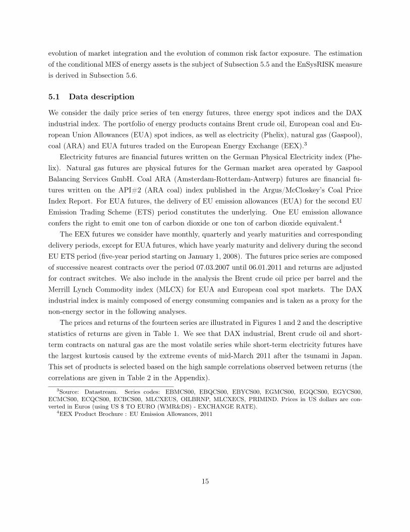
5.1 Data description

We consider the daily price series of ten energy futures, three energy spot indices and the DAXindustrial index. The portfolio of energy products contains Brent crude oil, European coal and Eu-ropean Union Allowances (EUA) spot indices, as well as electricity (Phelix), natural gas (Gaspool),coal (ARA) and EUA futures traded on the European Energy Exchange (EEX).3

Electricity futures are financial futures written on the German Physical Electricity index (Phe-lix). Natural gas futures are physical futures for the German market area operated by GaspoolBalancing Services GmbH. Coal ARA (Amsterdam-Rotterdam-Antwerp) futures are financial fu-tures written on the API#2 (ARA coal) index published in the Argus/McCloskey’s Coal PriceIndex Report. For EUA futures, the delivery of EU emission allowances (EUA) for the second EUEmission Trading Scheme (ETS) period constitutes the underlying. One EU emission allowanceconfers the right to emit one ton of carbon dioxide or one ton of carbon dioxide equivalent.4

The EEX futures we consider have monthly, quarterly and yearly maturities and correspondingdelivery periods, except for EUA futures, which have yearly maturity and delivery during the secondEU ETS period (five-year period starting on January 1, 2008). The futures price series are composedof successive nearest contracts over the period 07.03.2007 until 06.01.2011 and returns are adjustedfor contract switches. We also include in the analysis the Brent crude oil price per barrel and theMerrill Lynch Commodity index (MLCX) for EUA and European coal spot markets. The DAXindustrial index is mainly composed of energy consuming companies and is taken as a proxy for thenon-energy sector in the following analyses.

The prices and returns of the fourteen series are illustrated in Figures 1 and 2 and the descriptivestatistics of returns are given in Table 1. We see that DAX industrial, Brent crude oil and short-term contracts on natural gas are the most volatile series while short-term electricity futures havethe largest kurtosis caused by the extreme events of mid-March 2011 after the tsunami in Japan.This set of products is selected based on the high sample correlations observed between returns (thecorrelations are given in Table 2 in the Appendix).

3Source: Datastream. Series codes: EBMCS00, EBQCS00, EBYCS00, EGMCS00, EGQCS00, EGYCS00,ECMCS00, ECQCS00, ECBCS00, MLCXEUS, OILBRNP, MLCXECS, PRIMIND. Prices in US dollars are con-verted in Euros (using US $ TO EURO (WMR&DS) - EXCHANGE RATE).

4EEX Product Brochure : EU Emission Allowances, 2011

15

Name Underlying Maturity/ Mean Std. Dev. Skewness ExcessDelivery kurtosis

MPhelix Phelix (Physical 1/1 month -0.098 2.063 0.214 9.087QPhelix Electricity index) 1/1 quarter -0.036 1.454 0.895 11.123YPhelix 1/1 year -0.015 1.253 0.094 3.081MGaspool Natural Gas delivery 1/1 month -0.100 2.733 -0.236 2.875QGaspool in Gaspool area 1/1 quarter -0.071 2.307 0.212 2.308YGaspool 1/1 year -0.023 1.774 0.289 2.316MARA API#2 ARA 1/1 month 0.044 2.138 -0.617 3.461QARA coal index 1/1 quarter 0.016 2.104 -0.588 2.563YARA 1/1 year 0.036 1.815 -0.494 3.046YEUA Delivery of EU carbon 1 year/ -0.034 2.222 -0.276 3.005

emission allowances 2nd EU ETSEUA spot EUA spot index - -0.022 2.266 -0.048 2.860Brent Brent crude oil index - 0.042 2.329 -0.030 4.322Coal spot European coal spot index - 0.042 1.916 -0.494 2.243DAX industrial DAX industrial index - -0.013 2.322 -0.090 6.782

Table 1: Summary and descriptive statistics of returns. Sample period: 07.03.2007 - 06.01.2011(989 observations)

MPhelix (EUR/MWh)

2008 2010 2012

25

50

75

100MPhelix (EUR/MWh) QPhelix (EUR/MWh)

2008 2010 2012

25

50

75

100QPhelix (EUR/MWh) YPhelix (EUR/MWh)

2008 2010 2012

25

50

75

100YPhelix (EUR/MWh) MGaspool (EUR/MWh)

2008 2010 2012

10

20

30

MGaspool (EUR/MWh)

QGaspool (EUR/MWh)

2008 2010 2012

20

30

40 QGaspool (EUR/MWh) YGaspool (EUR/MWh)

2008 2010 2012

20

30

40

YGaspool (EUR/MWh) MARA (EUR/ton)

2008 2010 2012

50

100

150 MARA (EUR/ton) QARA (EUR/ton)

2008 2010 2012

50

100

150 QARA (EUR/ton)

YARA (EUR/ton)

2008 2010 2012

75

100

125

150 YARA (EUR/ton) YEUA (EUR/ton CO2e)

2008 2010 2012

10

20

30YEUA (EUR/ton CO2e) MLCX EUA spot (EUR/ton CO2e)

2008 2010 2012

100

150

200

MLCX EUA spot (EUR/ton CO2e) Brent crude oil (EUR/barrel)

2008 2010 2012

25

50

75

100 Brent crude oil (EUR/barrel)

MLCX European coal spot (EUR/ton)

2008 2010 2012

100

200

300

MLCX European coal spot (EUR/ton) DAX Industrial (EUR)

2008 2010 2012

2000

3000

4000DAX Industrial (EUR)

Figure 1: Prices. Sample period: 07.03.2007 - 06.01.2011 (989 observations). M, Q, Y letters beforethe names of futures contracts stand for monthly, quarterly and yearly maturity.

16

2008 2009 2010 2011

-10

0

10

20MPhelix returns (%)

2008 2009 2010 2011

0

10

QPhelix returns (%)

2008 2009 2010 2011

-5

0

5

YPhelix returns (%)

2008 2009 2010 2011

-10

0

10

MGaspool returns (%)

2008 2009 2010 2011

0

10

QGaspool returns (%)

2008 2009 2010 2011

-5

0

5

10 YGaspool returns (%)

2008 2009 2010 2011

0

10 MARA returns (%)

2008 2009 2010 2011

-5

0

5

10 QARA returns (%)

2008 2009 2010 2011

-5

0

5

10 YARA returns (%)

2008 2009 2010 2011

-10

0

10

YEUA returns (%)

2008 2009 2010 2011

0

10

EUA spot returns (%)

2008 2009 2010 2011

-10

0

10

20 Brent crude oil returns (%)

2008 2009 2010 2011

-5

0

5European coal spot returns (%)

2008 2009 2010 2011

-10

0

10

20 DAX Industrial returns (%) DAX Industrial returns (%)

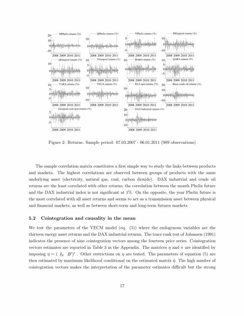
Figure 2: Returns. Sample period: 07.03.2007 - 06.01.2011 (989 observations)

The sample correlation matrix constitutes a first simple way to study the links between productsand markets. The highest correlations are observed between groups of products with the sameunderlying asset (electricity, natural gas, coal, carbon dioxide). DAX industrial and crude oilreturns are the least correlated with other returns; the correlation between the month Phelix futureand the DAX industrial index is not significant at 1%. On the opposite, the year Phelix future isthe most correlated with all asset returns and seems to act as a transmission asset between physicaland financial markets, as well as between short-term and long-term futures markets.

5.2 Cointegration and causality in the mean

We test the parameters of the VECM model (eq. (5)) where the endogenous variables are thethirteen energy asset returns and the DAX industrial returns. The trace rank test of Johansen (1991)indicates the presence of nine cointegration vectors among the fourteen price series. Cointegrationvectors estimates are reported in Table 3 in the Appendix. The matrices η and π are identified byimposing η = ( I9 B

�)� . Other restrictions on η are tested. The parameters of equation (5) arethen estimated by maximum likelihood conditional on the estimated matrix η. The high number ofcointegration vectors makes the interpretation of the parameter estimates difficult but the strong

17

significance5 of estimates indicates that all prices (including the DAX industrial index) contributeto the long-term price equilibrium.

In order to account for short-memory autocorrelation and causality up to the weekly lag (as inBillio and Caporin (2010)), we chose K and M of eq. (5) equal to five. The estimated coefficientsand robust6 standard errors of significant relationships at the 5% level are presented in Tables 4and 5 in the Appendix.7

The tables of estimation results show that the EUA spot index returns are not subject to error-correction. This result is in line with the results of Bunn and Fezzi (2008) and Fezzi and Bunn(2009) showing that carbon prices are weakly exogenous in the long run. Bunn and Fezzi (2008)explain this effect by the fact that carbon allowances are traded at the European level while otherproducts in the sample are exclusively traded in the German market area. For the same reason, itis not surprising that Brent crude oil is Granger-causal for EUA returns.

As expected, Brent crude oil returns are not caused by any variable. Conversely, Brent crude oilis causal for many other energy products (long-term Gaspool futures, coal spot, coal quarter futuresand EUA spot and futures returns). More surprising, the only variable explaining DAX industrialreturns is the quarter Phelix future; the estimated parameter is negative meaning that increasingelectricity futures prices have a negative impact on DAX industrial returns.

Granger-causality reflects the complex term structure of energy futures where the spot causesfutures returns but futures returns also cause spot returns (e.g. coal and EUA). Other relationshipsreflect the merit-order of electricity in Germany. The daily log demand for electricity is an exogenousvariable that explains the returns on the European coal spot index. Coal is usually referred as themarginal fuel for electricity generation during off-peak hours in Germany and it is significant toexplain returns of long-term electricity futures. The negative sign of the log demand is also asexpected; when electricity demand decreases coal spot prices decrease as well. Natural gas is themarginal fuel for peak load hours in Germany and it is significant to explain returns of short-termPhelix futures.

5.3 Causality in variances

The estimated coefficients and standard errors of significant relationships at the 5% level of theMultiplicative Causality GARCH model (eq. (6)) are reported in Tables 6 and 7 in the Appendix.8

Concerning the asymmetric parameter of the GJR model in (7), we find a positive estimate of γ

for the DAX industrial index and EUA products and a negative estimate for month Phelix futures.For the DAX industrial index, the parameter γ is the usual “leverage” parameter; negative shocks

5All estimates have t-values above 5 in absolute value.6Newey-West heteroskedasticity- and autocorrelation-consistent standard errors (HACSE)7The estimation results of this section are obtained using the PcGive module of OxMetrics version 6.10 (see

Doornik and Hendry (2009)).8These results and the results of the next sections are generated using Ox version 6.10 (see Doornik (2009)).

18

have a larger impact on volatility. For both DAX and EUA returns, this asymmetric effect is sostrong that the usual ARCH parameter is not significant anymore meaning that only the negativenews affect the volatility of these products. The negative estimate of γ for month Phelix futures isconsistent with the findings of Knittel and Roberts (2005) and Bauwens et al. (2012). Knittel andRoberts (2005) attribute this effect in electricity returns to the convexity of the supply function,since positive demand shocks have a larger impact on prices than negative demand shocks.

The interaction component that we define in (9) incorporates seasonal effects and causal rela-tionships. The EEX futures market closes during weekend days. Therefore, higher volatility is foundfor all EEX futures (except coal futures) at the beginning of the week (positive Monday effect). Theseasonality is different for the volatility of coal spot and futures returns where we find monthlyeffects.

Most causal relationships in the variances come from the year EUA future through the mul-tiplicative interaction component. The year EUA future is causal for electricity and short-termnatural gas futures. We find that higher Brent crude oil returns increase the volatility of long-termnatural gas futures. Causal relationships also take place between products with the same underlyingenergy but different maturities, as it is the case for electricity and coal.

From the results of the tests, causal relationships can be summarized through a network repre-sentation. The networks of causal relationships in the means (left part) and in the variances (rightpart) are illustrated in Figure 3. Arrows reflect the direction of causality.

Figure 3: Mean (left part) and variance (right part) causal networks: significant causal relationshipsat the 5% level. Sample period: 07.04.2007 - 06.01.2011 (988 observations)

19

5.4 Energy Market Integration and Systematic Risk

After removing causal relationships, we measure market integration or commonality among energyreturns due to the presence of common factors. Billio et al. (2010) show that commonality amongasset returns can be detected using a principal component analysis. From a restricted PCA on thesample correlation matrix of estimated standardized residuals ut, we obtain an industrial componentand an energy trend component (first and second principal components) that respectively accountfor 7% and 49% of the total variance of all energy and industrial assets. Three other principalcomponents have larger eigenvalues than the industrial component. The third component is highlycorrelated to coal assets and separates coal and Brent crude oil products from the other assets. Thefourth component opposes emission rights to natural gas, and natural gas futures have the highestcorrelations with this component. The fifth component is highly correlated to electricity short-termfutures. From the PCA on the sample correlation matrix, the cumulative contribution of the firstfour energy components accounts for 78%.

In order to assess the evolution of market integration, we measure the evolution of the cumulativepercentage of variance explained by the most important principal components (also called absorptionratio in Kritzman et al. (2011)). This measure can be interpreted as an aggregate measure ofcorrelations between products. Using a restricted dynamic PCA based on DCC correlations asdefined in Subsection (4.2), we show the evolution of market integration in Figure 4. The eigenvaluecontribution of the energy trend component is the most volatile, with values between 40% and 54%.

From Figure 4, we identify several events of market integration due to increasing correlations.These events are not necessarily inherent to the European energy market; they can either comefrom other sectors or other continents. The first event is due to the financial crisis; the eigenvaluecontribution of the first PC is higher during the years 2008-2009 with a peak in October 2008 (justafter the announcement of the Lehman Brothers bankruptcy in September 2008).

Winter 2009 was characterized by an extended period of cold weather, the spreading out ofthe effects of the financial turmoil to the real economy and a disruption in natural gas supplyfrom Russia (Kovacevic (2009)). The disruption arose from a commercial dispute between Russiaand Ukraine. The Russian gas supplier Gazprom refused to conclude a gas supply agreement for2009 with Ukraine until the Ukrainian gas company Naftogas fully repaid its debts to the Russiansupplier. As a result, from January 6, 2009, all natural gas supplies from Russia flowing via Ukrainewere cut off. Countries in Central and South Eastern Europe were the most affected. There was nosubstantial price increase on German natural gas markets but the volatility of prices increased asreserves were depleting at alarming speeds.9

Another event happens in April 2010 where the volatility of all EEX futures increased andespecially the volatility of natural gas futures. At the end of April, the maximum value of 10%return is reached for month and quarter Gaspool futures following the explosion of BP’s offshore

9Quarterly Report on European Gas Markets, QREGaM, Volume 2, Issue 1, January 2009 – Mars 2009.

20

oil-drilling platform, Deepwater Horizon, in the Gulf of Mexico on April 20, 2010. On April 26, thereturns of Gaspool futures surge; this date corresponds to the first trading day after April 23 wherethe complete information about BP’s oil leak had been transmitted to energy markets. In Europe,the shale gas industry was in its infancy but was expected to grow rapidly as shale gas representsan important unconventional fuel source for the future. The environmental disaster in the Gulf ofMexico indicated the possibility of tighter European regulation on shale gas drilling projects leadingto project delays and the consequent weakening of the natural gas industry.10

The last event of the sample happens in mid-March 2011 after the Japanese tsunami and thenuclear disaster of Fukushima on March 12. On March 14, the German Chancellor A. Merkelannounced a three-month moratorium on the extension of the lifetimes of 17 German nuclear powerplants. The next day, month and quarter Phelix futures returns reached their maximum and mostextreme values of 16% and 15% respectively.

2009 2010 2011

40

50

60

70

80

90

100

Ru

ssia

-Ukra

ine

NG

dis

pu

te

LB

ban

kru

ptc

y

BP

’s r

ig e

xp

losi

on

Fuku

shim

a p

lant

ou

tag

e

Hig

hes

t cr

ude

oil

pri

ce

1st Energy DPC contribution (%) 3 Energy DPCs contribution

2 Energy DPCs contribution 4 Energy DPCs contribution

Figure 4: Cumulative percentage of variance explained by the first four dynamic principal compo-nents associated to energy returns (contribution). Contribution of the first s−1 energy components:�s

j=2 λjt/�n

j=1 λjt .

Next to the aggregate measure of market integration, we are interested in measuring the marginalexposure of each product to the energy market risk factor. This marginal measure is interpreted

10BP’s Gulf of Mexico oil spill to affect EU shale gas projects, Energy Risk, May 2010.

21

as the systematic risk associated to the energy market and can be estimated by a correlation withthe energy market. In the dynamic PCA, dynamic correlations of the standardized residuals uit

with the principal component yjt are given by λjta2ijt. If we interpret the second component of

the restricted dynamic PCA as the energy market factor, the correlation with the energy trendcomponent (λEnMta

2i,EnMt) defines a measure of energy systematic risk.

Figure 5 shows the cross-sectional average correlations of each energy commodity class (elec-tricity, natural gas, coal, EUA, Brent crude oil) with the common energy market factor. Fromthe evolution of dynamic correlations, we can identify which asset contributed to market eventsobserved in Figure 4. For example, we observe that the systematic risk rises for Gaspool futuresduring April 2010 (BP’s oil spill) and Phelix futures during March 2011 (Fukushima accident). Thesystematic risk of emission rights also increases in March 2011. The demand for emission rightsis indeed expected to rise in Germany as short run replacement capacitiy for nuclear generation ismainly composed of old gas-fired power plants. The German decision to move away from nuclearenergy did not however impact the systematic risk of primary energy commodities according to thismeasure.

2009 2010 2011

0.6

0.7

0.8 Cor(Electricity, Energy Market)

2009 2010 2011

0.6

0.7

0.8 Cor(Natural Gas, Energy Market)

2009 2010 20110.7

0.8

0.9 Cor(Coal, Energy Market)

2009 2010 2011

0.4

0.6

0.8 Cor(Carbon, Energy Market)

2009 2010 2011

0.2

0.4

0.6

Cor(Brent, Energy Market)

Figure 5: Energy Systematic Risk: correlations of standardized returns ut with the energy trendcomponent. Correlations are average correlations per energy commodity class (Electricity, NaturalGas, Coal, EUA, Brent crude oil).

22

Note that the systematic risk attached to crude oil is probably underestimated due to thecomposition of the initial set of energy products selected for the analysis. The set includes severalproducts of each energy commodity class but only one crude oil index. If we want to measure thesystematic risk of crude oil using this methodology, we should more equally balance the initial setof products. However, if the goal is to measure the systematic risk associated to EEX products, thechoice of energy products in our application appears to be adequate.

5.5 The conditional MES of energy assets

We turn to the estimation of the conditional MES of EEX futures. This measure is an adaptedversion of the conditional MES of Brownlees and Engle (2011) accounting for causality, commonfactor exposure and sensitivity to extreme events in energy markets. The conditional means µit

and the conditional variances σ2it incorporate the causal relationships identified with the augmented

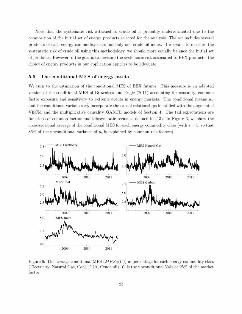
VECM and the multiplicative causality GARCH models of Section 4. The tail expectations arefunctions of common factors and idiosyncratic terms as defined in (13). In Figure 6, we show thecross-sectional average of the conditional MES for each energy commodity class (with s = 5, so that86% of the unconditional variance of ut is explained by common risk factors).

2009 2010 2011

2.5

5.0

7.5MES Electricity

2009 2010 2011

2.5

5.0

MES Natural Gas

2009 2010 2011

2.5

5.0

7.5

MES Coal

2009 2010 2011

2.5

5.0

7.5 MES Carbon

2009 2010 2011

0.0

2.5

5.0 MES Brent

Figure 6: The average conditional MES (MESit(C)) in percentage for each energy commodity class(Electricity, Natural Gas, Coal, EUA, Crude oil). C is the unconditional VaR at 95% of the marketfactor.

23

The conditional MES for the German energy market appears to be higher for coal and emissionrights and lower for crude oil with this measure. The MES of crude oil may be underestimatedcompared to the MES of EEX futures for the same reasons discussed in the section on systematicrisk. However, in absence of a ’real crisis’ in the sample (the identified ’market events’ are onlymoderately bad days as described by Acharya et al. (2010)), it is difficult to assess the quality ofthe estimated conditional MES.

The MES increases for all EEX futures after the financial crisis due to high volatility of energymarkets when oil prices started to plummet. Some futures reach a maximal MES at the beginning ofJanuary 2009 when returns became highly positive due to the combination of several adverse events(economic downturn, unusual cold winter, and gas supply disruptions in Europe). The release ofthe information about BP’s oil leak had an impact on the MES of all futures but this impact seemsto be more important for natural gas futures. The German political reaction following Fukushimaevents had a major impact on short-term electricity futures but is also visible on carbon emissionrights. Not shown here, the conditional MES is also larger for short-term futures because of theirhigh volatility and high sensitivity to extreme market events.

5.6 Estimated Energy Systemic Risk

In a final step, the conditional MES is used to derive the Energy Systemic Risk measure (EnSys-RISK) as we define it in (2). This measure represents the total cost in million euros of each energycommodity class to the German non-energy sector during a potential energy crisis and is illustratedin Figure 7. The EnSysRISK measure is a conditional measure and evolves dynamically based onpast information about quantities and prices.

The quantity exposure is approximated by the final consumption, assuming no reserves availableto the non-energy sector. Therefore, the energy systemic risk measure will probably be overestimatedfor storable energy commodities. The expected final consumption is the final consumption of thelast month and it is assumed that the only available energy products for the end consumers are theenergy assets we considered in our analysis.

Most energy products seem to be characterized by an increasing trend of systemic risk as pricesand systemic prices are increasing. The systemic risk of natural gas has a seasonal pattern wheresystemic risk increases during winter, as natural gas is an important heating fuel in Germany. Thesystemic risk of natural gas is high in winter 2009 with the disruption in European gas supply, butis even higher in winter 2011. The systemic risk of emission rights follows the seasonal patternof natural gas. There is a peak in the systemic risk measure of electricity in March 2011 but themeasure reverts to its pre-Fukushima level in May 2011. The increase of systemic risk after theFukushima accident is also present in all other energy commodities, except crude oil.

24

2009 2010 2011

75

100

125

150 EnSysRISK Electricity

2009 2010 2011

20

40

60

EnSysRISK Natural Gas

2009 2010 2011

2

4

6

EnSysRISK Coal

2009 2010 2011

10

15

20

25 EnSysRISK Carbon

2009 2010 2011

50

100

150EnSysRISK Brent

Figure 7: Energy Systemic Risk measure (EnSysRISK) in million euros for each energy class (Elec-tricity, Natural Gas, Coal, EUA, Crude oil).

6 Conclusion

The existence of systemic risk in energy markets may be subject to discussions and different under-standings. In this paper, we discuss, define and measure the systemic risk associated to an energycrisis. Our energy systemic risk measure (EnSysRISK) represents the total cost of an energy prod-uct to the rest of the economy during an energy crisis. A high degree of dependence of the economyon energy will increase the EnSysRISK measure.

EnSysRISK is a function of the Marginal Expected Shortfall (MES). We adapt the conditionalMES of Brownlees and Engle (2011) to account for the co-movements in the means, the variancesand the tail expectations of energy assets. The systemic event is defined by an extreme positiveenergy market shock from the supply side; we are therefore measuring the upper-tail dependencebetween the energy product and the energy market in the cases where the non-energy returns arenegative.

Our definition of the MES allows for linear and non-linear causal relationships in the conditionalmeans and variances. Tail expectations are a function of common risk factors and idiosyncraticterms. We estimate the dynamic linear and tail dependence of energy returns on the market and

25

analyze the impact of several energy market events (Russia-Ukraine gas dispute, BP’s oil leak,Fukushima power plant outage). Finally, from the estimated conditional MES and the final con-sumption quantities, we derive the EnSysRISK measure and find increasing energy systemic risk forall energy products.

This analysis of systemic risk in the energy market is a first attempt to understand how systemicrisk may be present in such markets. We provide a methodology to organize and understand thecomplex dependence of energy assets. Further research opportunities are left open. Forecasting theMES is probably the most important. One-day ahead forecasts are straightforward to obtain fromour methodology. Long-run forecasts are also possible to obtain from a simulation procedure asdescribed in Brownlees and Engle (2011). The long-term horizon in the energy sector is howeverlonger than in the financial sector; forecasts over six months may not be enough to help investmentdecisions in generation capacitity. The long-term of the energy sector is also subject to technologyand regulatory changes that are difficult to incorporate into a forecasting exercise. Other dimensionsfor systemic risk propagation in the energy market are to explore; the most important one being thetransmission between regional markets. Then, the impact of energy systemic risk on other marketssuch as equity markets may also be interesting to study.

References

Acharya, V., L. Pedersen, T. Philippon, and M. Richardson (2010). Measuring systemic risk.Working Paper Stern School of Business.

Adrian, T. and M. Brunnermeier (2010). CoVaR. Federal Reserve Bank of New York Staff ReportsNo. 348.

Alexander, C. (2002). Principal component models for generating large GARCH covariance matrices.Economic Notes 31:2, 337–359.

Barsky, R. and L. Kilian (2004). Oil and the macroeconomy since the 1970s. NBER Working PaperNo. 10855.

Battiston, S., D. Delli Gatti, M. Gallegati, B. Greenwald, and J. Stiglitz (2009). Liaisons dan-gereuses: increasing connectivity, risk sharing, and systemic risk. NBER Working Paper No.15611.

Bauwens, L., C. Hafner, and D. Pierret (2012). Multivariate volatility modeling of electricity futures.Journal of Applied Econometrics , forthcoming.

Benink, H. A. (1995). Coping with Financial Fragility and Systemic Risk, Volume 30 of Financial

and Monetary Policy Studies. Kluwer Academic Publishers.

26

Benth, F. E. and P. Kettler (2010). Dynamic copula models for the spark spread. Quantitative

Finance 11:3, 407–421.

Billio, M. and M. Caporin (2010). Market linkages, variance spillovers, and correlation stability:Empirical evidence of financial contagion. Computational Statistics and Data Analysis 54, 2443–2458.

Billio, M., M. Getmansky, A. Lo, and L. Pelizzon (2010). Econometric measures of systemic risk inthe finance and insurance sectors. NBER Working Paper No. 16223.

Boerger, R. H., A. Cartea, R. Kiesel, and G. Schindlmayr (2009). Cross-commodity analysis andapplications to risk management. Journal of Futures Markets 29:3, 197–217.

Brownlees, C. and R. Engle (2011). Volatility, correlation and tails for systemic risk measurement.NYU Working Paper.

Bunn, D. and C. Fezzi (2008). A vector error correction model of the interactions among gas,electricity and carbon prices: An application to the cases of Germany and United Kingdom. InMarkets for Carbon and Power Pricing in Europe: Theoretical Issues and Empirical Analyses,pp. 145–159. Francesco Gulli.

Caporin, M. (2007). Variance (non) causality in multivariate GARCH. Econometric Reviews 26:1,1–24.

Carpantier, J. (2010). Commodities inventory effect. CORE Discussion Paper 2010/40.

Carruth, A., M. Hooker, and A. Oswald (1998). Unemployment equilibria and input prices: Theoryand evidence from the united states. Review of Economics and Statistics 28, 621–628.

Chevallier, J. (2012). Time-varying correlations in oil, gas and CO2 prices: an application usingBEKK, CCC and DCC-MGARCH models. Applied Economics 44:32, 4257–4274.

Doornik, J. (2009). An Object-Oriented Matrix Language Ox 6. Timberlake Consultants Press.

Doornik, J. and D. Hendry (2009). Modeling Dynamic Systems Using PcGive 13: Volume II.Timberlake Consultants Press.

Emery, G. and Q. Liu (2001). An analysis of the relationship between electricity and natural gasfutures prices. The Journal of Futures Markets 22, 95–122.

Engle, R. (2002). Dynamic conditional correlation: a simple class of multivariate generalized autore-gressive conditional heteroskedasticity models. Journal of Business and Economic Statistics 20:3,339–350.

27

Engle, R. and J. Rangel (2008). The spline-GARCH model for low-frequency volatility and its globalmacroeconomic causes. Review of Financial Studies 21:3, 1187–1222.

Escribano, A., I. Pena, and P. Villaplana (2011). Modeling electricity prices: International evidence.Oxford Bulletin of Economics and Statistics 73:5, 622–650.

Fezzi, C. and D. Bunn (2009). Structural interactions of european carbon trading and energy prices.The Journal of Energy Markets 2:4, 53–69.

Forbes, K. and Rigobon (2002). No contagion, only interdependence: measuring stock marketco-movements. The Journal of Finance 57:5, 2223–2261.

Glosten, L., R. Jagannathan, and D. Runkle (1993). On the relation between the expected value andthe volatility of the nominal excess return on stocks. The Journal of Finance 48:5, 1779–1801.

Gronwald, M., J. Ketterer, and S. Trück (2011). The relationship between carbon, commodity andfinancial markets - a copula analysis. Economic Record 87, 105–124.

Haldrup, N. and M. Nielsen (2006). A regime switching long memory model for electricity prices.Journal of Econometrics 135:1-2, 349–376.

Hamilton, J. (1983). Oil and the macroeconomy since World War II. The Journal of Political

Economy 91:2, 228–248.

Hamilton, J. (2003). What is an oil shock? Journal of Econometrics 113, 363–398.

Hamilton, J. (2011). Historical oil shocks. University of California, San Diego Working Paper.

Hautsch, N., J. Schaumburg, and M. Schienle (2011). Financial network systemic risk contributions.SFB 649 Discussion Paper 2011-072.

Johansen, S. (1991). Estimation and hypothesis testing of cointegration vectors in Gaussian vectorautoregressive models. Econometrica 59, 1551–1580.

Joskow, P. and J. Parsons (2012). The future of nuclear power after Fukushima. MIT CEEPRWorking Paper 2012-001.

Kato, K. (2012). Weighted Nadaraya-Watson estimation of conditional expected shortfall. Journal

of Financial Econometrics 10:2, 265–291.

Knittel, C. and M. Roberts (2005). An empirical examination of restructured electricity prices.Energy Economics 27, 791–817.

Kovacevic, A. (2009). The impact of the Russia-Ukraine gas crisis in South Eastern Europe. Tech-nical report, Oxford Institute for Energy Studies.

28

Kritzman, M., Y. Li, S. Page, and R. Rigobon (2011). Principal components as a measure ofsystemic risk. Journal of Portfolio Management 37-4, 112–126.

Lautier, D. and F. Raynaud (2011). Systemic risk in energy derivative markets: a graph-theoryanalysis. University Paris-Dauphine.

Lee, K.and Ni, S. (2002). On the dynamic effects of oil price shocks: a study using industry leveldata. Journal of Monetary Economics 49-4, 823–852.

Nelson, D. B. (1991). Conditional heteroskedasticity in asset returns: a new approach. Economet-

rica 59, 349–370.

Ng, V., R. Engle, and M. Rothschild (1992). A multi-dynamic-factor model for stock returns.Journal of Econometrics 52, 245–266.

Perron, P. (1989). The great crash, the oil price shock, and the unit root hypothesis. Journal of

Political Economy 57, 1361–1401.

Rangel, J. and R. Engle (2009). The factor-spline-GARCH model for high and low frequencycorrelations. Banco de Mexico Working Paper No. 2009-03.

Rotemberg, J. and M. Woodford (1996). Imperfect competition and the effects of energy priceincreases on economic activity. Journal of Money, Credit and Banking 28:4, 549–577.

Scaillet, O. (2004). Nonparametric estimation and sensitivity analysis of expected shortfall. Math-

ematical Finance 14, 115–129.

Scaillet, O. (2005). Nonparametric estimation of conditional expected shortfall. Insurance and Risk

Management Journal 74, 639–660.

Tieben, B., M. Kerste, and I. Akker (2011). Curtailing commodity derivative markets: what arethe consequences for the energy sector? Technical report, SEO Economic Research.

Tsay, R. S. (2005). Analysis of Financial Time Series (Second ed.). Wiley Series in Probability andStatistics. John Wiley & Sons.

Zaleski, P. (1992). Industry concentration and the transmission of cost-push inflation: Evidencefrom the 1974 OPEC oil crisis. Journal of Economics and Business 2, 135–141.

29

Appendix

Correlation matrix

Phelix Month 1Phelix Quarter 0.79 1

Phelix Year 0.53 0.79 1Gaspool Month 0.37 0.40 0.37 1Gaspool Quarter 0.39 0.47 0.48 0.81 1

Gaspool Year 0.36 0.53 0.63 0.63 0.78 1Coal ARA Month 0.31 0.48 0.63 0.31 0.37 0.47 1Coal ARA Quarter 0.33 0.52 0.66 0.33 0.40 0.51 0.94 1

Coal ARA Year 0.31 0.51 0.67 0.32 0.40 0.54 0.88 0.93 1EUA Year 0.27 0.42 0.57 0.23 0.30 0.37 0.27 0.29 0.30 1

EUA spot index 0.26 0.39 0.52 0.20 0.28 0.34 0.25 0.27 0.28 0.93 1Brent crude oil 0.12 0.24 0.42 0.14 0.21 0.38 0.33 0.37 0.40 0.30 0.30 1Coal spot index 0.30 0.48 0.61 0.30 0.40 0.50 0.83 0.88 0.85 0.31 0.32 0.44 1DAX industrial 0.07 0.14 0.28 0.09 0.13 0.19 0.23 0.24 0.23 0.28 0.28 0.36 0.28 1

Table 2: Correlation matrix of returns. Sample period: 07.03.2007 - 06.01.2011 (989 observations)

Cointegration results

η1 η2 η3 η4 η5 η6 η7 η8 η9

Phelix Month 1Phelix Quarter 1

Phelix Year 6.640 5.097 2.979 2.503 -0.342 1.734 5.358Gaspool Month 1Gaspool Quarter 1

Gaspool Year 4.588 3.493 -1.799Coal ARA Month 1Coal ARA Quarter 1

Coal ARA Year -12.668 -4.583 -6.121 -6.681 -6.818 -5.380 0.546 -5.049EUA Year -2.091 -2.682 -2.057 -0.292 -0.426 -0.976 -2.106

EUA spot index 1Brent crude oil 6.824 2.997 3.945 4.911 3.620 -0.513 3.551Coal spot index 1DAX industrial 1

Table 3: Estimated cointegration vectors (η). Sample period: 07.03.2007 - 06.01.2011 (989 obser-vations)

30

Augmented VECM results

Coefficient HACSE t-valuePhelix Month Cst 12.694 4.669 2.72

Wednesday (ϕ) 0.235 0.087 2.71Phelix Quartert−1 (δ1) 0.125 0.042 2.97Gaspool Montht−1 (δ1) 0.084 0.020 4.19

η�2yt−1 (π) -0.363 0.142 -2.55

η�9yt−1 (π) -0.937 0.309 -3.04

Phelix Quarter Cst 7.485 2.956 2.53Phelix Quartert−1 (δ1) 0.096 0.029 3.29

Gaspool Quartert−1 (δ1) 0.032 0.011 2.79Coal spot indext−1 (δ1) 0.053 0.015 3.46

η�2yt−1 (π) -0.441 0.096 -4.58

η�9yt−1 (π) -0.688 0.192 -3.59

Phelix Year Cst 10.802 2.622 4.12Coal spot indext−1 (δ1) 0.061 0.015 4.16EUA spot indext−1 (δ1) 0.048 0.009 5.27

η�2yt−1 (π) -0.304 0.078 -3.88

η�9yt−1 (π) -0.789 0.167 -4.72

Gaspool Month Cst 14.673 3.993 3.67Gaspool Quartert−1 (δ1) 0.166 0.029 5.83

MA(Coal ARA Year returns, 5) -0.278 0.061 -4.53η�1yt−1 (π) 0.403 0.138 2.92

η�3yt−1 (π) -1.438 0.379 -3.79

Gaspool Quarter Cst -3.325 3.393 -0.98Gaspool Montht−1 (δ1) 0.088 0.015 6.05

Coal ARA Quartert−3 (δ3) -0.063 0.016 -3.92Brent crude oilt−5 (δ5) -0.053 0.017 -3.19

η�1yt−1 (π) 0.674 0.148 4.56

η�3yt−1 (π) -0.879 0.215 -4.09

η�4yt−1 (π) -0.984 0.296 -3.33

η�9yt−1 (π) 1.162 0.268 4.34

Gaspool Year Cst 0.994 0.348 2.86Phelix Yeart−1 (δ1) 0.080 0.033 2.42

Coal spot indext−1 (δ1) 0.048 0.022 2.22Brent crude oilt−1 (δ1) 0.043 0.014 3.01

η�4yt−1 (π) -0.887 0.163 -5.43

η�8yt−1 (π) 0.683 0.128 5.33

Coal ARA Month Cst 10.084 2.196 4.59Coal ARA Yeart−1 (δ1) -0.165 0.052 -3.17Coal spot indext−1 (δ1) 0.378 0.058 6.52

η�3yt−1 (π) -0.332 0.095 -3.51

η�7yt−1 (π) -2.871 0.766 -3.75

η�9yt−1 (π) -0.269 0.092 -2.94

Table 4: Augmented VECM model estimates of eq. (5) (1/2). MA(xt, τ) is a moving average ofvariable xt over the past τ days. Sample period: 07.04.2007 - 06.01.2011 (988 observations)31

Coefficient HACSE t-valueCoal ARA Quarter Cst 1.250 0.469 2.67

Coal ARA Yeart−1 (δ1) -0.189 0.043 -4.41Coal spot indext−1 (δ1) 0.393 0.050 7.87Brent crude oilt−1 (δ1) -0.026 0.008 -3.42

η�5yt−1 (π) 5.729 0.884 6.45

η�6yt−1 (π) -7.674 1.203 -6.38

Coal ARA Year Cst -0.458 0.340 -1.35Coal ARA Yeart−1 (δ1) -0.132 0.050 -2.63Coal spot indext−1 (δ1) 0.269 0.052 5.21

η�4yt−1 (π) -0.429 0.104 -4.11

η�8yt−1 (π) 0.539 0.117 4.60

EUA Year Cst -8.357 2.541 -3.29Brent crude oilt−1 (δ1) -0.136 0.031 -4.34EUA spot indext−1 (δ1) 0.622 0.041 15.1

EUA Yeart−1 (δ1) -0.449 0.054 -8.32η�7yt−1 (π) 5.193 1.605 3.24

η�8yt−1 (π) 0.752 0.225 3.34

EUA spot index Cst -0.002 0.068 -0.032EUA Yeart−1 (δ1) 0.144 0.0410 3.57

Brent crude oilt−1 (δ1) -0.132 0.031 -4.23EUA Yeart−2 (δ2) 0.388 0.045 8.59EUA Yeart−3 (δ3) 0.207 0.038 5.44

EUA spot indext−2 (δ2) -0.397 0.049 -8.18EUA spot indext−3 (δ3) -0.208 0.037 -5.68

Brent crude oil Cst 6.124 1.610 3.80η�3yt−1 (π) -0.786 0.206 -3.82

Coal spot index Cst 20.909 6.072 3.44Coal spot indext−1 (δ1) -0.124 0.043 -2.89Coal spot indext−2 (δ2) -0.193 0.034 -5.65Brent crude oilt−1 (δ1) -0.054 0.013 -4.08

Coal ARA Quartert−1 (δ1) 0.321 0.036 9.01Coal ARA Quartert−2 (δ2) 0.181 0.032 5.68

Electricity daily demandt−1 (θ1) -1.224 0.402 -3.04η�5yt−1 (π) 10.764 1.899 5.67

η�6yt−1 (π) -9.155 1.724 -5.31

η�8yt−1 (π) -5.329 1.365 -3.90

DAX industrial index Cst 48.802 8.972 5.44Phelix Quartert−1 (δ1) -0.140 0.051 -2.75

η�1yt−1 (π) -2.581 0.559 -4.62

η�2yt−1 (π) 1.632 0.486 3.36

η�5yt−1 (π) 12.2098 3.048 4.01

η�8yt−1 (π) -11.238 3.590 -3.13

η�9yt−1 (π) -4.065 0.703 -5.78

Table 5: Augmented VECM model estimates of eq. (5) (2/2) . Sample period: 07.04.2007 -06.01.2011 (988 observations)

32

Multiplicative Causality GARCH results

Coefficient Std. error t-valuePhelix Month Cst (c) 2.935 1.435 2.046

ARCH (α) 0.175 0.033 5.256GARCH (β) 0.845 0.028 30.341

GJR (γ) -0.073 0.034 -2.159Monday (κ) 0.815 0.102 8.004

EUA Year (α) 0.283 0.059 4.774Phelix Year (ϑ) 0.156 0.044 3.564

Phelix Quarter Cst (c) 1.208 0.375 3.224ARCH (α) 0.122 0.023 5.428

GARCH (β) 0.856 0.024 36.061Monday (κ) 0.711 0.103 6.922

EUA Year (α) 0.270 0.066 4.062Phelix Month (α) 0.152 0.070 2.178Phelix Year (ϑ) 0.156 0.045 3.490

Phelix Year Cst (c) 1.175 0.336 3.501ARCH (α) 0.121 0.023 5.324

GARCH (β) 0.859 0.025 34.238Monday (κ) 0.418 0.101 4.148

EUA Year (ϑ) 0.209 0.041 5.150Gaspool Month Cst (c) 10.054 4.965 2.025

ARCH (α) 0.104 0.015 6.992GARCH (β) 0.891 0.016 57.003Monday (κ) 0.658 0.104 6.333April (κ) 0.589 0.225 2.617

Coal ARA Month (ϑ) 0.169 0.045 3.715EUA Year (α) 0.169 0.072 2.339

Gaspool Quarter Cst (c) 5.177 0.980 5.283ARCH (α) 0.139 0.031 4.507

GARCH (β) 0.803 0.039 20.412Monday (κ) 0.441 0.105 4.205

May (κ) -0.594 0.230 -2.577Brent crude oil (ϑ) 0.123 0.044 2.814

Gaspool Year Cst (c) 2.686 0.380 7.066ARCH (α) 0.063 0.015 4.077

GARCH (β) 0.907 0.021 42.397Monday (κ) 0.385 0.108 3.553

Brent crude oil (ϑ) 0.152 0.042 3.588

Table 6: Multiplicative Causality GARCH model estimates of eq. (6) (1/2). Sample period:07.04.2007 - 06.01.2011 (988 observations)

33

Coefficient Std. error t-valueCoal ARA Month Cst (c) 3.834 0.954 4.019

ARCH (α) 0.111 0.022 5.152GARCH (β) 0.865 0.026 33.205Thursday (κ) -0.386 0.105 -3.655January (κ) 0.888 0.233 3.813August (κ) -0.882 0.234 -3.775

Coal spot index (ϑ) 0.140 0.044 3.215Coal ARA Quarter Cst (c) 3.379 0.750 4.508

ARCH (α) 0.097 0.022 4.453GARCH (β) 0.880 0.027 32.585January (κ) 0.794 0.232 3.426August (κ) -0.754 0.225 -3.359

Coal ARA Month (ϑ) 0.146 0.043 3.426Coal ARA Year Cst (c) 2.148 0.486 4.424

ARCH (α) 0.088 0.020 4.415GARCH (β) 0.893 0.025 36.374

Phelix Month (α) 0.159 0.065 2.439EUA Year Cst (c) 3.845 0.775 4.960

ARCH (α) 0.031 0.017 1.832GARCH (β) 0.898 0.023 38.240

GJR (γ) 0.093 0.027 3.378Monday (κ) 0.214 0.102 2.107

Coal ARA Year (ϑ) 0.151 0.042 3.582EUA spot index Cst (c) 4.509 0.857 5.260

ARCH (α) 0.037 0.018 2.045GARCH (β) 0.901 0.026 35.162

GJR (γ) 0.072 0.026 2.814Brent crude oil Cst (c) 3.988 0.762 5.236

ARCH (α) 0.042 0.009 4.782GARCH (β) 0.947 0.011 85.526

Coal spot index Cst (c) 3.045 0.776 3.926ARCH (α) 0.114 0.021 5.374

GARCH (β) 0.862 0.025 34.357January (κ) 0.767 0.240 3.195

DAX industrial index Cst (c) 4.912 1.558 3.152ARCH (α) 0.022 0.016 1.369

GARCH (β) 0.909 0.017 52.986GJR (γ) 0.109 0.035 3.139

Gaspool Year (ϑ) 0.134 0.047 2.869

Table 7: Multiplicative Causality GARCH model estimates of eq. (6) (2/2). Sample period:07.04.2007 - 06.01.2011 (988 observations)

34