the suitability of low-cost measurement systems for
TRANSCRIPT

FACULTY OF TECHNOLOGY
THE SUITABILITY OF LOW-COST
MEASUREMENT SYSTEMS FOR ROLLING
ELEMENT BEARING VIBRATION MONITORING
Jarno Junnola
Supervisors: Erkki Jantunen (VTT Technical Research Centre of Finland
Ltd.) Toni Liedes (University of Oulu)
MECHANICAL ENGINEERING
Master’s Thesis
March 2017

ABSTRACT
The Suitability of Low-Cost Measurement Systems for Rolling Element Bearing
Vibration Monitoring
Jarno Junnola
University of Oulu, Degree Programme of Mechanical Engineering
Master’s thesis 2017, 79 p. + 41 p. Appendixes
Supervisors at the university: Toni Liedes
The aim of this thesis is to study if inexpensive vibration monitoring systems could be
suitable for condition monitoring of rolling element bearings and if they could be able to
detect bearing defects at an early stage. As a starting point the following set of
requirements for the system have been defined: the system should be priced below 100
€, it should be able to measure the vibrations reaching up to 10 000 Hz frequencies and
the amplitude resolution of the system should be at minimum 16-bits. The ability of the
system to be part of internet of things (IoT) is also seen as a positive thing and an
advantage. While searching for an adequate system, a market review consisting low-
cost vibration monitoring devices and low-cost vibration monitoring components has
been done. A secondary aim of the work is to highlight the impact of different
components of the signal chain to the measured vibration signal itself and familiarize
the reader with the signal chain found in vibration monitoring.
To fulfill the main objective of the thesis, a broad market review was performed and it
was mainly done by searching the Internet. Experimental tests for the low-cost
equipment were also done to find out their real competence. The suitability of the found
components were tested in various ways including calibrations of accelerometers and an
investigation of the capability of Raspberry Pi 3 model B single board computer. The
capability of Raspberry to act as a platform for accelerometers and its ability to sample
the incoming high-frequency signals from accelerometers were checked. The effects of
the vibration monitoring components to the gathered data were examined through
simulations done with math software called Mathcad. The literature review that was
carried out is used to introduce the signal path of the vibration monitoring signal hand in
hand with the simulations.

The results of the work include state-of-the-art information of low cost vibration
monitoring devices and introduction to some not so familiar vibration monitoring
options that may have the potential to be used in bearing condition monitoring. The
documented signal chain simulation models shown in the appendixes contribute to the
understanding of vibration signal chain and allow for their further use. The conclusion
of this thesis is that a 100 € budget is too tight for a high-quality and general-purpose
vibration monitoring device for early bearing defect detection.
Keywords: condition monitoring, bearings, vibration

TIIVISTELMÄ
The Suitability of Low-Cost Measurement Systems for Rolling Element Bearing
Vibration Monitoring
Jarno Junnola
Oulun yliopisto, Konetekniikan tutkinto-ohjelma
Diplomityö 2017, 79 s. + 41 s. liiteitä
Työn ohjaaja yliopistolla: Toni Liedes
Työn tavoitteena on tutkia kykeneekö edullinen värähtelynmittauslaitteisto
vierintälaakereiden kunnonvalvontaan ja laakerivian aikaiseen tunnistamiseen.
Lähtökohtana annettujen vaatimuksien mukaan laitteiston tulisi olla hinnaltaan alle 100
€, sen olisi kyettävä mittamaan värähtelyä yltäen jopa 10 000 Hz taajuuksiin ja
laitteiston amplitudiresoluution tulisi olla minimissään 16-bittiä. Myös laitteiston kyky
olla osa laitteiden Internetiä (internet of things; IoT) katsotaan eduksi. Kykenevää
laitteistoa etsiessä työssä esitellään myös katsaus tällä hetkellä markkinoilta löytyviin
edullisiin värähtelymittauslaitteisiin ja värähtelymittauskomponentteihin. Toissijaisena
tavoitteena työssä on tuoda esille värähtelymittauslaitteistoissa olevien komponenttien
vaikutus värähtelysignaaliketjuun ja mittauslaitteistolla saatuun dataan sekä perehdyttää
lukijaansa värähtelysignaaliketjuun.
Päätavoitteen täyttämiseksi suoritettiin laaja markkinakatsaus pääosin Internetiä
käyttäen. Myös markkinoilta löydettyjen värähtelymittauskomponenttien soveltuvuutta
testattiin kokeellisesti muun muassa edullisia kiihtyvyysantureita kalibroiden sekä
tutkien Raspberry Pi 3 model B - yhden piirilevyn tietokoneen ominaisuuksia. Työssä
arvioitiin ja testattiin Raspberryn kykenevyyttä toimia alustana kiihtyvyysantureille ja
kyvykkyyttä näytteistää kiihtyvyysantureilta tulevaa korkeataajuuksista signaalia.
Värähtelymittauskomponenttien vaikutusta värähtelysignaaliin ja siitä saatavaan
informaation tutkittiin Mathcad -laskentaohjelmalla tehtyjen simulointien myötä.
Värähtelysignaaliketjuun tutustuttiin simulointien lisäksi ja simulointien tukena
kirjallisuuskatsauksen muodossa.

Työn tuloksena saavutettiin laaja katsaus tämän hetken edullisiin
värähtelymittauslaitteistoihin ja tuotiin esiin myös mahdollisesti hieman
tuntemattomiakin värähtelymittausratkaisuja, joilla voi olla potentiaalia
kunnonvalvonnan värähtelymittauksiin. Työn liitteenä olevat signaaliketjun
simulointimallit edesauttavat ymmärtämään värähtelymittauksen signaaliketjua sekä
mahdollistavat myös niiden jatkokäytön. Työ myös paljastaa, että 100 € budjetti on liian
tiukka laadukkaaseen ja yleiskäyttöiseen värähtelymittaukseen perustuvaan
vierintälaakereiden kunnonvalvontalaitteeseen.
Asiasanat: kunnonvalvonta, laakerit, värähtely

PREFACE
This Master's thesis was done for VTT Technical Research Centre of Finland Ltd during
the end of the year 2016 and the beginning of the year 2017. The objective of the thesis
was to figure out the available low-cost vibration monitoring systems and their
capability for vibration monitoring of rolling element bearings
I want to thank VTT for giving me this opportunity to write the thesis and be part of the
company, and my supervisors Erkki Jantunen from VTT and Toni Liedes from the
university of Oulu. Also I want to thank Jouni Laurila from the university of Oulu for
examining the thesis.
Oulu, 19.04.2017
Jarno Junnola

TABLE OF CONTENTS
ABSTRACT
TIIVISTELMÄ
PREFACE
TABLE OF CONTENTS
LIST OF ABBREVIATIONS
1 INTRODUCTION ............................................................................................................ 10
1.1 Research questions and objectives ............................................................................. 10
1.2 Contents of the thesis ................................................................................................. 11
1.3 Scientific contribution of the thesis ............................................................................ 12
2 CONDITION MONITORING .......................................................................................... 13
2.1 Financial benefits ....................................................................................................... 13
2.2 Safety aspects ............................................................................................................. 14
2.3 Rolling element bearing condition monitoring .......................................................... 14
2.3.1 Vibration monitoring ........................................................................................ 15
2.3.2 Temperature monitoring ................................................................................... 18
2.3.3 Lubrication monitoring ..................................................................................... 19
3 COMPONENTS OF A VIBRATION MONITORING SYSTEM ................................... 21
3.1 Accelerometers ........................................................................................................... 22
3.1.1 Piezoelectric ...................................................................................................... 22
3.1.2 Piezo film .......................................................................................................... 23
3.1.3 MEMS............................................................................................................... 24
3.2 Amplifiers .................................................................................................................. 25
3.3 Filters.......................................................................................................................... 28
3.3.1 Anti-Aliasing Filters ......................................................................................... 29
3.4 Analogue-to-digital converters ................................................................................... 32
3.4.1 Flash/Parallel ADC ........................................................................................... 36
3.4.2 Successive Approximation (SAR) ADC .......................................................... 36
3.4.3 Sigma-Delta (ΣΔ) ADC .................................................................................... 37
3.5 Processors ................................................................................................................... 37
4 MARKET REVIEW ......................................................................................................... 40
4.1 Accelerometers ........................................................................................................... 40
4.2 Measurement system from integrated circuits ........................................................... 42
4.3 Smart Sensors ............................................................................................................. 44
4.4 Single-board computers and microcontrollers ........................................................... 47

4.5 Evaluation boards for ADCs, filters and amplifiers ................................................... 49
4.6 USB/Ethernet DAQs .................................................................................................. 51
5 TESTS FOR LOW-COST EQUIPMENT ........................................................................ 53
5.1 Accelerometers ........................................................................................................... 53
5.1.1 ACH 01 ............................................................................................................. 57
5.1.2 ADXL001 ......................................................................................................... 59
5.2 Raspberry Pi 3 as a sensor platform ........................................................................... 63
5.2.1 Communication between Raspberry and external hardware ............................ 64
5.2.2 Programming Raspberry ................................................................................... 66
5.2.3 Raspberry & EVAL-AD7609 ........................................................................... 66
6 DISCUSSION ................................................................................................................... 70
7 SUMMARY ...................................................................................................................... 73
8 REFERENCES .................................................................................................................. 74
APPENDIXES:
Appendix 1. Mathcad Prime 3 model of shock signal & ADC
Appendix 2. Basics of a signal path and processing modeled with Mathcad Prime 3
Appendix 3. Accelerometers.
Appendix 4. ADC ICs.
Appendix 5. Single-board computers.
Appendix 6. Evaluation boards for IC ADCs.
Appendix 7. USB DAQs and oscilloscopes.
Appendix 8. Certificate of calibration (wax mounting): B&K 4394.
Appendix 9. Certificate of calibration (wax mounting): Te Connectivity ACH 01.
Appendix 10. Certificate of calibration (glue mounting): Analog devices ADXL001.
Appendix 11. Certificate of calibration (screw mounting): Analog devices ADXL001.

LIST OF ABBREVIATIONS
ADC Analogue-to-Digital Converter
AFE Analogue Front End
ALU Arithmetic and Logic Unit
AMP Amplifier
ASIC Application Specific Integrated Circuit
CPU Central Processing Unit
DAC Digital-to-analogue converter
DSC Digital Signal Controller
DSP Digital Signal Processing
DSP Digital Signal Processors
FPGA Field Programmable Gate Arrays
GPIO General-Purpose Input-Output
I/O Input/Output
I2C Inter-Integrated Circuit
I2S Inter-IC Sound
IC Integrated Circuits
IDE Integrated Development Environment

IoT Internet of Things
MCU Microcontroller Unit
MEMS Micro Electro Mechanical Systems
MISO Master-In Slave-Out
MOSI Master-Out Slave-In
OP-AMP Operational Amplifier
PCB Printed Circuit Board
SAR Successive Approximation
SBC Single-Board Computer
SBM Single-Board Microcontroller
SoC System on a Chip
SPI Serial Peripheral Interface
Sps Samples per second
SS Slave Select
UART Universal Asynchronous Receiver/Transmitter
USB Universal Serial Bus
10
1 INTRODUCTION
Vibration monitoring is the most used method in condition monitoring of rotating
machines and it can also be used in operational control and troubleshooting (Nohynek,
Lumme 2004, p. 17). Bearings are seen as one the most critical parts defining the health
of machines and their remaining lifetime in current production machines (El-Thalji
2016, p.11). The condition of a bearing is usually followed by monitoring vibrations
and normally accelerometers are used as instruments to sense the vibrations (Tandon,
Choudhury 1999, p.469 & p.474, Safizadeh, Latifi 2014, p.2).
Unfortunately, the total price of a vibration monitoring device for detecting bearing
faults may be a five figure number which motivates the search for cheaper options
(TEquipment 2017). The decrease in price of vibration monitoring devices makes it
economically beneficial to carry out vibration monitoring also with assets that do not
cause so huge risks to production or to safety. When introducing condition monitoring
to new machines there is always the financial question i.e. does the company gain or
lose with condition monitoring. The gain is usually measured in money and thus the
price of the measuring equipment has a meaning. The gain could also be a safer working
environment or better product quality earned through condition monitoring.
1.1 Research questions and objectives
Inspired from few euro accelerometers that have come to market, like LIS2DH and
LIS2DS12 from STMicroelectronics, it is interesting to know if these low-cost
accelerometers are capable to be used in condition monitoring of rolling element
bearings. Consequently, the first research question is: Are accelerometers cheaper than
10 euros capable to be used in rolling element bearing condition monitoring
applications for early defect detection?
A low-cost complete measurement system for bearings from accelerometer to processed
vibration signal was another motivation. Are there complete measurement systems
which can measure signals up to 10 000 Hz with a minimum resolution of 16-bit and are

11
these available under 100 euros. It was also hoped that the measurement system would
have some sort of readiness level for IoT. The second research question is: Is it possible
to get a vibration monitoring system under 100 euros that is capable to measure signals
with frequency content up to 10 000 Hz, to give processed vibration signal information
of bearing faults and is connectable to be a part of internet of things?
Related to the previous questions, the third question handles about what kind of
parameters measurement devices have and what kind of meaning do they have related to
the gathered data. The third question is: What is the meaning of individual vibration
monitoring components (ADC, filter, amplifier etc.) in signal chain and how do they
affect to the gathered information?
In summary, it can be said that the main objective of this thesis is to find out if it is
possible to do bearing condition monitoring with really cost-effective equipment. To
reach this main objective, a number of secondary objectives have to be reached:
evolution of bearing faults have to be known at some state, the needed properties for
bearing measurement devices have to be defined so that the devices are able to detect
bearing failures in an early stage and a market review has to be done to get the
knowledge of the available measurement systems and components nowadays.
1.2 Contents of the thesis
The thesis covers areas from explaining why condition monitoring is done to the
availability of low-cost bearing monitoring systems. The thesis tries to shed light on
which kind of components are included in vibration measurement devices, which kind
of properties do these components have, which kind of changes come to measurement
results if these properties are changed and which kind of properties are needed from
vibration measurement device components to be used in the rolling element bearing
condition monitoring. The following content of the thesis is divided into six chapters to
cover the subjects mentioned:
12
- Chapter 2 explains why condition monitoring is done and presents ways how
rolling element bearing condition monitoring is done including vibration
monitoring, temperature monitoring and lubricant analysis.
- Chapter 3 explains the features of different measurement device components and
shows their effect on measuring results.
- Chapter 4 summarizes the market review of vibration measurement devices.
- Chapter 5 presents the testing of Raspberry Pi3, EVAL-AD7609, ADXL001 and
ACH 01.
- Chapter 6 discusses about the results gained from chapters 4, 5 and 6.
- Chapter 7 offers the thesis summary and proposals for future work.
1.3 Scientific contribution of the thesis
This thesis shows the current state of cheap vibration measuring devices and possible
few considerable low-cost approaches to be used in vibration based condition
monitoring. Some of the vibration monitoring components are simulated and the
simulation methods are described in the appendixes. Simulations clarify the suitability
of different kind of vibration monitoring devices.
13
2 CONDITION MONITORING
Condition monitoring tools are used in Condition Based Maintenance to analyse the
current health condition of an asset and consequently, set up proper preventive
maintenance schedules (Bengtsson 2004, p.1) . Without knowing the state or the usage
of the machine it is impossible to do condition based or predictive maintenance.
Condition monitoring has shown a huge positive effect on increasing the utilization rate
of machines and increasing profitableness (Nohynek, Lumme 2004, p.7 & p.11). The
profits of condition monitoring are an increase in productivity, a better possibility to do
scheduled/planned maintenance, a better utilization of downtime, a decrease in
unplanned shutdowns and an increase in the lifetime of machines (Nohynek, Lumme
2004, p.11).
2.1 Financial benefits
By sacrificing working hours and financial resources to condition monitoring gives
huge savings from maintenance (Nohynek, Lumme 2004, p.13). By doing the condition
monitoring right, it decreases unexpected shutdowns, decreases unnecessary machine
openings, reduces the need for big spare part storages and shortens the unavoidable,
planned and necessary downtimes (Nohynek, Lumme 2004, p.13). Downtimes can be
divided in two parts: waiting time and maintenance time (Nohynek, Lumme 2004,
p.12). Waiting time consists of noticing the failure, picking up the proper documents for
the case, reserving personnel to do the maintenance, reserving tools for maintenance,
reserving spare parts from a storage and purchasing spare parts if those cannot be found
from storage (Nohynek, Lumme 2004, p.12). Just after following all the previous steps
that are included in the waiting time it is possible to start the maintenance itself.
All of the tasks of the waiting time can be done while processes are running if condition
monitoring is used and thus shorten the downtime and consequently save money. Also,
the maintenance time itself can be reduced if condition monitoring is applied. The
maintenance time reduction comes from the facts that maintenance can be planned more

14
precisely when the failure is known beforehand and failures can be fixed before they
grow for more serious breakdowns.
Other financial benefit comes from the decrease of unplanned shutdowns. When there
are fewer shutdowns, the usage times of machines are higher and, therefore, the
availability of the asset increases. This way the Overall Equipment Efficiency also
increases, thus, increasing the profitability. In most cases, unplanned shutdowns can be
reduced more than 50 % when moving from corrective maintenance to condition
monitoring based maintenance (Nohynek, Lumme 2004, p.12).
2.2 Safety aspects
Machine failures or improper use can cause very expensive financial loses, but more
importantly, the worst scenario would be if the personnel get injured. Machines with
high safety risks are equipped with measurement systems i.e. condition monitoring
systems that control the machine by themselves. For example, if a failure or malfunction
is detected the safety system can shut down the machine or otherwise put it in safe-
mode and consequently prevent expensive failures or personnel injuries (Nohynek,
Lumme 2004, p.15). Typical systems among others that have this kind of safety systems
are turbines, compressors, machines with pistons, grinders and big electric motors
(Nohynek, Lumme 2004, p.15). Consequently, in generalization big, expensive and high
revolution rate machines usually have safety systems.
2.3 Rolling element bearing condition monitoring
Historically condition monitoring was mainly done using senses: bearings were listened
using a wooden stick, temperatures of machines were felt by hands, vibrations of
machines were checked by hands or feet and so on (Nohynek, Lumme 2004, p.13).
Also, the quality of the manufactured products was one way to follow the condition of
production machinery (Nohynek, Lumme 2004, p.13). These previously used methods
have still a place in condition monitoring and they should not be underestimated but,
nowadays, condition monitoring is based on different measuring methods (Nohynek,
Lumme 2004, p.13). Rolling element bearings are mainly monitored using three

15
methods: vibration monitoring, temperature monitoring and wear debris analysis which
includes lubrication analysis (Tandon, Choudhury 1999, p.469). Out of those three
previously mentioned methods vibration monitoring is the most used one (Tandon,
Choudhury 1999, p.469). The following paragraph will introduce all of these three
methods.
2.3.1 Vibration monitoring
Vibration monitoring is the most used method and when used correctly it is the best
condition monitoring method to follow the condition of a rotating machine (Nohynek,
Lumme 2004, p.17, Shahzad, Cheng et al. 2013, p.670). Vibration monitoring can also
be used for operation control to adjust the parameters of a process. Also because of the
wide usage and the effectiveness of vibration monitoring, this thesis will mainly focus
on this method.
To detect rolling element bearing failure in an early stage of failure evolution, vibration
monitoring should be done in the natural frequency area of a bearing. Natural
frequencies are better information sources of defect than commonly followed bearing
fault frequencies in an early stage because amplitudes of fault frequencies are so small
in the beginning of degradation and because of the phenomenon called slippage (El-
Thalji 2016, pp. 46-47). Slippage causes that impacts do not follow the fault frequencies
so accurately and thus the amplitudes of fault frequencies do not increase in the matter
that they are expected to increase. When the rolling element passes the early stage fault,
the contact and the impact between rolling elements and raceways might awake the
natural frequencies of bearing raceways and thus it is wise to monitor the natural
frequencies of bearing raceways to detect bearing failures in an early stage. A rough
estimation of natural frequency of a raceway can be calculated with the following
equation (1):
ω=E/(πD) (1)
where E is the speed of sound in the material and D is the diameter of a raceway (Sassi,
Badri et al. 2007). If more information like the moment of inertia of the race cross
section, the mass per unit length and/or the cross-sectional constant of a bearing is

16
available, then more accurate functions, that are collected together also by El-Thalji
(2016, pp.46-47), can be used when calculating natural frequencies.
The mentioned goal of this thesis to find a measurement system that is capable to
measure up to 10 000 Hz signals would lead to a system which is capable to measure
the natural frequencies of steel bearings from diameter 3 cm upwards. The capability to
measure 10 000 Hz signals means of course that an ADC has to fulfill the Nyquist
theorem and it has to be able to sample at least 20 000 samples per second (Gatti,
Ferrari 2002, pp.754-755). In comparison, a system with the capability to measure 1 000
Hz signals would lead to a device which could detect natural frequencies starting from
30 cm diameter bearings. Diameters are calculated with equation (1) firstly solving the
diameter out of the equation and then putting variables in place. When we know that E
is 5900 m/s in steel, ω = 2πf and f is 10 000 Hz or 1000 Hz in these cases, we can
calculate the diameter in the following way (J. Johansson, P. e. Martinsson et al. 2007,
p.1980, Mäkelä 2008, p.95):
D = E/ (ωπ) = E / (2πf × π) = 5900 / (2π×10000 × π) ≈ 0,030 m,
D = E/ (ωπ) = E / (2πf × π) = 5900 / (2π×1000 × π) ≈ 0,299 m.
There are plenty of vibration monitoring methods but those can be categorized into two
classes: the first class methods are used for monitoring overall vibrations and simple
statistical vibration signal parameters of rolling bearings while the second class methods
are more focused on monitoring detailed vibration and a wider range of bearing
parameters (Nohynek, Lumme 2004, p.18). With the first class methods it is normal to
use two vibration measurement devices: one device to monitor overall vibration in the
range of 10 Hz – 1000 Hz and a second one to measure frequencies typically above
2000 Hz. The overall vibration in the frequencies from 10 Hz to 1000 Hz roughly
reveals the problems related to a rotating shaft such as imbalance, misalignment and
looseness of connections (Nohynek, Lumme 2004, p.18). The second measuring device
to monitor frequencies above 2000 Hz is mainly used to detect rolling element bearing
failures. It should be noted that vibration in high frequencies noticeably increase when
lubrication is poor in rolling bearing, an indentation occurs or when other bearing
failures appear (Nohynek, Lumme 2004, p.18). The second measurement device might

17
also be an ultrasonic measurement device which is used to detect bearing failures but
also to detect gas and liquid leakages (Nohynek, Lumme 2004, p.18). First class
methods are sensitive enough to monitor simple machines which do not have multiple
shafts spinning at multiple speeds (Nohynek, Lumme 2004, p.18).
When machines have multiple shafts with different rotational speeds and/or power
transmission units, the second class measurement devices must be used. The first class
devices are not able to separate different vibration sources from each other and it is hard
to detect the source of the problem (Nohynek, Lumme 2004, p.18). For example, high
overall vibration levels could be caused by a big unbalance in some of the shafts, a
misalignment error, a bearing failure, a looseness of mounting, a resonance of a
structure or the cavitation of a pump, but the first class equipment are not capable to
locate the source (Nohynek, Lumme 2004, p.18). In these more complex cases one or
various multichannel spectrum analyzers is needed.
With a spectrum analyzer it is possible to separate different frequencies and their
amplitudes from the signal. Different frequencies are caused by different parts of the
machine and thus it is conceivable to follow the state of different machine components
pretty reliably (Nohynek, Lumme 2004, p.19). Spectrum analyzers enable the analysis
and more complex monitoring that uses signal analysis methods like envelope analysis,
phase-analysis and cepstrum analysis (Nohynek, Lumme 2004, p.19).
Kuntoon perustuva kunnossapito – handbook (title translation in English: Condition
Based Maintenance) has a different approach in categorizing vibration monitoring
devices: vibration pens and other basic handheld meters, portable data collectors,
multiple channel FFT analyzers and PC based measurement devices and permanently
mounted online analyzers & data collectors (Miettinen, Miettinen et al. 2009, pp.259-
263). Vibration pens and other basic handheld meters measure one or multiple
parameters (most commonly overall velocity of vibration from a fixed bandwidth) and
they can have data transferring and storing capabilities. Vibration pens and other basic
handheld meters can be used for very basic condition monitoring carried out for
example by an operator while operating a machine. Portable data collectors usually have
a large memory, a display and a wide variety of frequency and time domain tools for

18
signal analysis. Portable data collectors can be used by their own or in an interaction
with a computer. Multiple channel FFT analyzers and PC based measurement devices
have commonly 8-64 channels, very high sample rate and very wide range of signal
analysis tools. Multiple channel FFT analyzers and PC based measurement devices are
used in case of difficult vibration problems and their usage needs expertise and
theoretical knowledge. Permanently mounted online analyzers and data collectors are
used with machines that need to be often monitored or the measurement needs to be
continuous. Permanently mounted online analyzers and data collectors have usually
versatile tools for signal analysis and signal plotting.
PSK standardisation registered association has also their own perspective to
categorizing vibration monitoring devices. PSK 5705 standard categorizes vibration
monitoring devices depending on the installation on the measurement location:
permanently mounted, half-fixed and portable devices/systems. Permanently mounted
and portable devices are easily understandable but half-fixed means that sensors are
permanently fixed in place but they are measured with portable device. PSK 5710
standard categorises measurement devices into 4 types depending on their signal and
data processing capabilities. Type 1 devices measure the total/overall level of vibration
and one parameter is showing that value. Type 2 devices measure High frequencies
(typically above 5000 Hz) and the level of vibration is expressed with maximum of two
parameters. Type 3 devices have selectable frequency bandwidth and the measured
vibration can be expressed in time or frequency domain. Type 4 measurement systems
are able to do failure detection and even to do prediction about the safe usage time left.
2.3.2 Temperature monitoring
There are three types of temperature sensors available: touch type, infrared thermometer
and infrared camera (Nohynek, Lumme 2004, p.20). Touch type thermometers are the
simplest ones to use. With touch type thermometers the user does not have to worry
about emission factors of materials or about possible interference caused by reflecting
heat waves (Nohynek, Lumme 2004, p.20). The disadvantages of touch type
thermometers are that they need quite long settling times and that there is not always a
possibility to touch the monitored location (Nohynek, Lumme 2004, p.20).

19
With infrared thermometers it is possible to measure temperatures from a distance up to
100 meters away from the monitored location (Nohynek, Lumme 2004, p.20). It is
worth noting that the distance will affect the accuracy of the measurement. Infrared
thermometers have wider usability range than touch type thermometers. The possibility
to measure temperature from a distance has made it easier to use thermometers for
example to monitor electric components. Infrared thermometers have been used for a
long time to monitor electric components such as, fuses, switches and transformers
If there is a need to measure temperature from multiple spots near to each other
simultaneously then infrared camera is the best method (Nohynek, Lumme 2004, p.21).
The needed knowledge about different interference sources is greater with infrared
camera and also with infrared thermometer than with a touch thermometer. With
infrared cameras and thermometers, the user must take in consideration emission factors
of different materials and colours, different heat reflections especially from reflecting
surfaces and also the rate of accuracy when measured from a distance.
Temperature measurements were popular with bearing monitoring but because they
were not able to detect the failure early enough, they have been replaced with different
methods like vibration monitoring (Nohynek, Lumme 2004, p.20, Li, Liang et al. 2015).
Because almost all faults emit a noticeable amount of heat once the failure is in a more
serious stage, it is good to use temperature measurements as a secondary or supportive
monitoring method (Nohynek, Lumme 2004). Temperature monitoring is used for
example to observe unbalance load or bad condition of rollers of paper machines, valve
leakages or poor lubrication of seals (Nohynek, Lumme 2004, p.21).
2.3.3 Lubrication monitoring
Lubrication analysis is one way to monitor the condition of machines and it is done by
taking samples from the lubricant oil, lubricant grease or even from hydraulic oil
(Miettinen, Miettinen et al. 2009, p.428). Lubricant analysis can bring information about
the wearing of parts of a machine, the operation of a process, the effectiveness of the
lubricant and even the lubricant condition itself (Miettinen, Miettinen et al. 2009,
p.428). By following the amount of particles in a lubricant, the material of particles and

20
by measuring the size and the shape of particles it is possible to notice how harsh the
wear of the machine is, what components of the machine are suffering from wear and
how the components wear (abrasion, removal of chips etc.) (Nohynek, Lumme 2004,
p.23, Miettinen, Miettinen et al. 2009, pp.432-436). In the normal state when lubricated
surfaces are moving against each other the particle size could be about 10 micro meters
but when the wearing is severe the amount of particles rises notably and the sizes of
particles could be 10 to 100 times larger than in the normal state (Nohynek, Lumme
2004, p.23).
With lubricant analysis it is possible to detect gearbox and hydraulic system failures at
an early stage (Miettinen, Miettinen et al. 2009, p.429). Also, it is claimed that in many
cases the lubricant analysis detects a beginning failure earlier than basic vibration
measurements like the overall vibration measurements do (Miettinen, Miettinen et al.
2009, p.435 & 437). According to Miettinen et al. (2009, p.429), a very powerful
condition monitoring system is achieved if lubricant analysis is combined with vibration
measurements and especially if also process parameters (like speed and load) are
followed at the same time.
Instead of manual particle counting there are also less time consuming options
available. As a different method to determine the amount of particles or solids in a
lubricant is to measure the mass of solids in a very thin membrane after the oil has gone
through it (Miettinen, Miettinen et al. 2009, p.431). Automated counters are also
available which can count the complete number of particles in lubricant and also count
the number of particles of different size (Miettinen, Miettinen et al. 2009, p.432).

21
3 COMPONENTS OF A VIBRATION MONITORING
SYSTEM
In Figure 1 can be seen a basic block diagram of digital data acquisition (DAQ) system.
First a physical signal is sensed with a sensor/transducer. Electrical components always
introduce some noise into a signal and so do also transducers/sensors. After the physical
phenomenon is converted to an electrical signal with a transducer, the signal goes to the
signal conditioning block. Signal conditioning includes amplifying, filtering and
impedance matching between the transducer and an analogue-to-digital converter
(ADC). When transducer´s properties are improved in the signal conditioning block it is
time to feed the signal to an ADC. In the ADC the signal is quantized and the signal
gets a binary or digital representation. When the signal is in digital format it can be read
by a processor which could be for example inside of a computer. The digital signal can
be analysed, stored, processed digitally (e.g. using Fast Fourier Transform) and/or
graphs of the signal can be plotted to the user. The following paragraphs will explain
each of these blocks more in detail and also describe the key features of each
component involved in a vibration monitoring signal chain from the vibrating
component to the processor.
Figure 1. Digital Data Acquisition System (Zarate 2016).

22
3.1 Accelerometers
An accelerometer is a transducer which produces a current or a voltage value
proportional to the acceleration level to which it is exposed to (Broch 1980, p.100).
There are different designs to reach this accelerometer definition and the following
chapters will introduce some of the designs.
Accelerometers have characteristics which specify their properties: transfer function,
sensitivity, measurement range, linearity, noise, bandwidth and resonant frequency are
some of the used qualifying factors for accelerometers (Urban 2016, pp.396-397,
Wilson 2005, p.151). A transfer function tells the relation between the measured
voltage/charge and the acceleration level. Sensitivity is the factor defining how much
voltage or current is produced per acceleration unit and it can be measured in mV/g. The
measurement range character defines the overall acceleration range in g’s that the
accelerometer can measure. Linearity defines the maximum error from a linear transfer
function over the specified measurement range. Noise tells the amount of unwanted
distortion that every sensor produces to the output signal. Bandwidth states the
frequency range of vibration that the accelerometer is able to catch. Resonant frequency
of the accelerometer is one of the factors that define the bandwidth of the accelerometer.
3.1.1 Piezoelectric
A piezoelectric accelerometer is the most common accelerometer type and it is broadly
used in vibration analysis (Wilson 2005, p.137). The functionality of a piezoelectric
accelerometer is based on the piezoelectric material inside of them. These piezoelectric
elements are usually made of quartz or artificially polarized polycrystalline ceramic
(Broch 1980, p.100, Wilson 2005, p.141). When a piezoelectric material is compressed,
stretched or sheared, it generates an electric charge on the surface. This kind of charge
creation is called the piezoelectric effect (Urban 2016, pp.104-105). To capture this
electric charge, at least two electrodes are needed.
A seismic mass inside a piezoelectric accelerometer is attached to the piezoelectric
material and when exposed to acceleration the mass starts to move and shares,
compresses or stretches the piezoelectric material (Broch 1980, p.100). The voltage or
23
charge coming out of the accelerometer is relative to the acceleration it is subjected to.
By following the voltage/charge and knowing the transfer function it is possible to
know the acceleration level.
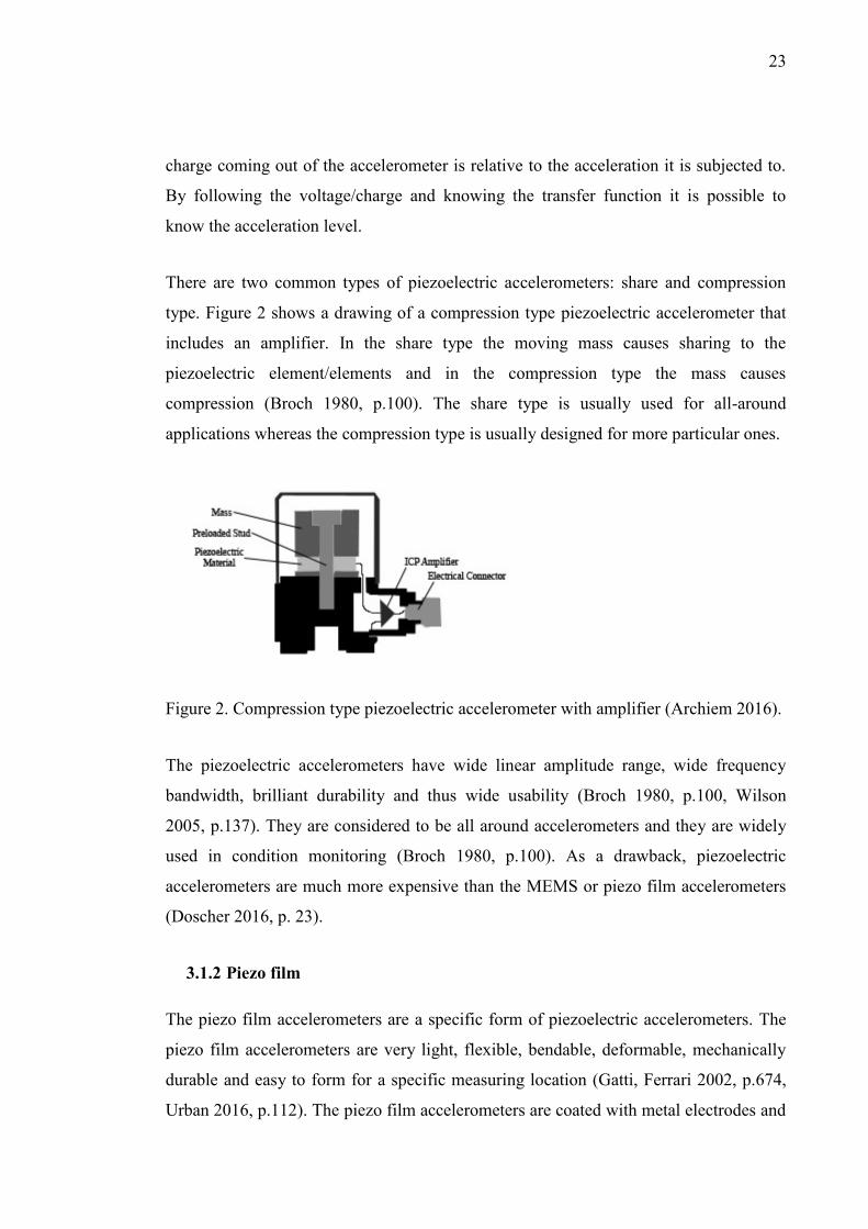
There are two common types of piezoelectric accelerometers: share and compression
type. Figure 2 shows a drawing of a compression type piezoelectric accelerometer that
includes an amplifier. In the share type the moving mass causes sharing to the
piezoelectric element/elements and in the compression type the mass causes
compression (Broch 1980, p.100). The share type is usually used for all-around
applications whereas the compression type is usually designed for more particular ones.
Figure 2. Compression type piezoelectric accelerometer with amplifier (Archiem 2016).
The piezoelectric accelerometers have wide linear amplitude range, wide frequency
bandwidth, brilliant durability and thus wide usability (Broch 1980, p.100, Wilson
2005, p.137). They are considered to be all around accelerometers and they are widely
used in condition monitoring (Broch 1980, p.100). As a drawback, piezoelectric
accelerometers are much more expensive than the MEMS or piezo film accelerometers
(Doscher 2016, p. 23).
3.1.2 Piezo film
The piezo film accelerometers are a specific form of piezoelectric accelerometers. The
piezo film accelerometers are very light, flexible, bendable, deformable, mechanically
durable and easy to form for a specific measuring location (Gatti, Ferrari 2002, p.674,
Urban 2016, p.112). The piezo film accelerometers are coated with metal electrodes and

24
also protecting plastic can be used (Measurement Specialties 1999). The piezo films are
commonly made out of polyvinylidene fluoride (PVDF/PVF2) which is shaped in thin
layers (Gatti, Ferrari 2002, p.674).
3.1.3 MEMS
MEMS acronym comes from the words Micro Electro Mechanical Systems. There are
different MEMS sensors for different applications. For example, it is possible to find
MEMS gyroscopes, MEMS accelerometers and MEMS pressure sensors from the
markets. With the term MEMS sensors it is meant sensors that are made using the same
kind of manufacturing methods as with integrated circuits (IC) called semiconductor
manufacturing processes (Frank 2013, p.1). MEMS are often highly integrated
apparatuses which combine microelectronics and micro machined structures together
(Frank 2013, p.9). By using these semiconductor manufacturing processes it is possible
to produce a lot of sensors to one wafer at once and thus get a low price tag for a single
sensor (Miettinen, Miettinen et al. 2009, p.244).
The MEMS sensors are tiny and light in weight and thus they are good in measuring
locations where the accelerometer must be light and the size must be small (Agoston
2012, p.278). The MEMS accelerometers’ functionality is based usually either
capacitive or piezoresistive phenomenon (McGrath, Scanaill 2013, p.21). The capacitive
MEMS accelerometers have capacitor plates attached to a spring with a suspended mass
which is capable to move when the accelerometer is subjected to acceleration. Other
capacitor plates are anchored in place and when the mass moves the gap between the
anchored and the attached capacitor plates changes and so changes the capacitor’s
geometry and the capacitance which is measured (Agoston 2012, p.278).
The piezoresistive MEMS accelerometers have piezoresistive material attached to
cantilever beams which move when the accelerometer is exposed to acceleration. When
the beams deform their resistive properties change and this change is proportional to the
acceleration level (McGrath, Scanaill 2013, p.21). The change in resistivity is measured
and the level of acceleration is derived from the measured change (McGrath, Scanaill
2013, p.20).
25
3.2 Amplifiers
An amplifier´s basic task is to amplify the incoming signal while introducing low
electrical noise or other errors like offset and gain error. Amplifiers have also other
purposes: improving the signal to noise ratio, being a frequency filter, being an
impedance matching block and being an isolator between a sensor and the rest of the
coming circuit after the sensor (Urban 2016, p.199). Amplifiers can be made from
components (semiconductors, resistors, capacitors, inductors etc.) but there are also
readymade amplifier integrated circuits in which these components are already included
(Urban 2016, p.198).
After amplifying the signal, it goes to a filter and to an ADC. An amplifier enables the
use of the resolution of the ADC more efficiently even with low level signals. There are
different types of amplifiers available: operational amplifiers, programmable-gain
amplifiers, instrumentation amplifiers, programmable-gain instrumentation amplifiers,
chopper amplifiers, isolation amplifiers etc. (Measurement Computing corp. 2012,
pp.39-47, Wilson 2005, p.45). The simulations shown in Figure 3 - Figure 6 show the
effect of amplification to the gained information. The simulations are done with math
software called Mathcad and the whole simulations can be found in appendices 1 and 2.
Some of the parameters shown in appendices 1 and 2 (including for example the gain)
need to be changed to match the different cases.
In Figure 3 and Figure 4 the effect of amplification is simulated by using a sine signal
with an added shock signal which simulates the impulses generated by bearing defects.
The impulse vibrates at 3000 Hz. The raw signal is shown in blue and the sampled
signal in red in both figures. The analogue to digital conversion is done with an 8-bit
ADC which has the input range from -5 volts to +5 volts. In Figure 3, the signal is
sampled without amplification and in Figure 4 the signal is amplified by a factor of 10
(please notice the scales of figures). The amplification can be also expressed as decibels
which is often the case.

26
Figure 3. Analogue to digital conversion for an unamplified signal.
Figure 4. Analogue to digital conversion for a signal which is amplified by a factor of
10.

27
In Figure 5 and Figure 6 the previously shown signals can be seen in the frequency
domain and it can also be seen how the information at high frequencies is lost if the
signal is sampled without proper amplification. The information at high frequencies is
very important for early bearing defect detection (Nohynek, Lumme 2004, p.18, El-
Thalji 2016, p.46). Interestingly a phenomenon of FFT and sidebands is also more
clearly shown in the spectrum of the amplified signal.
Figure 5. Spectrum from unamplified signal.
Figure 6. Spectrum from signal which is amplified by a factor of 10.

28
Operational amplifier or OP-AMP is seen as one of the principle building blocks for
amplifiers (Urban 2016, p.199). A good OP-AMP has the following features: high input
resistance (measured in GΩ), low output resistance (a fraction of ohms), ability to drive
capacitive loads without becoming unstable, low input offset voltage, low bias current,
very high open-loop gain (up to 10^4 – 10^6), low noise, high operating bandwidth and
low sensitivity to power supply and environmental variations (Urban 2016, pp.199-
200).
The mentioned open-loop gain is frequency depended and it also changes according to
variations in the supply voltage, load and temperature (Urban 2016, p.200). This open-
loop instability is the reason why the OP-AMPs are rarely used in the open-loop mode.
Usually the OP-AMPs are used with feedback components in a so called closed-loop
mode which improves the gain stability, linearity and output impedance (Urban 2016,
p.201). As a rule of thumb, it is said that the closed-loop gain should be 100 times
smaller than the open-loop gain at the highest frequency of interest for moderate
accuracy and 1000 times smaller for more accurate needs (Urban 2016, p.201).
3.3 Filters
The most common filter types are Butterworth, Bessel and Chebyshev (Measurement
Computing corp. 2012, p.47, Gaura, Newman 2006, p.131). All of these can be used for
low-pass, high-pass, band-pass and band-reject filtering (Measurement Computing corp.
2012, p.47). Low-pass filtering means the attenuation of high frequencies. High-pass
filtering means the opposite to the low-pass filtering: attenuation of low frequencies.
Band-pass filtering allows a certain bandwidth of frequencies to go through but
attenuates the rest. Band-reject filtering attenuates a certain frequency bandwidth but
lets the rest go through.
All of the three filter types have their own characteristics. Butterworth has the flattest
passband but it introduces a non-linear phase response (Measurement Computing corp.
2012, p.48, Gaura, Newman 2006, p.131). Chebyshev has the steepest attenuating curve
but it has a ripple effect before the cutting point frequency, ring effect with a step
response and even more non-linear phase response than Butterworth (Measurement

29
Computing corp. 2012, p.48, Gaura, Newman 2006, p.131). Bessel is something in
between the two previous ones. Bessel does not have a steep response curve but is has
the best phase linearity and step response (Measurement Computing corp. 2012, p.48,
Gaura, Newman 2006, p.131). In Figure 7 are shown the low-pass filter responses for
different filter types. The Chebyshev type I filter is shown in blue, the Bessel in red and
the Butterworth in yellow. All the shown filters are modeled using Mathcad’s own filter
functions and all of them have the cut off frequency at 10 Hz which is marked with a
dash line. The simulation for filters can be found in appendix 2.
Figure 7. Chebyshev I, Bessel & Butterworth filter gain responses (cut-off at 10 Hz).
3.3.1 Anti-Aliasing Filters
Aliasing is a phenomenon that occurs when a signal is not sampled with a high enough
sample rate. The Nyquist theorem says that a signal should be sampled at least twice as
fast as the signal’s highest frequency (Gatti, Ferrari 2002, pp.754-755). If the Nyquist
theorem is not followed, high signals will be reflected to low frequencies when sampled
and this will ruin the sampled result and this phenomenon will be difficult to notice
from the result (Gatti, Ferrari 2002, pp.754-756). In Figure 8 and Figure 9 the anti-
aliasing phenomenon is simulated. This simulation was done in a similar way that is
shown in appendix 2 with a little variation: in this simulation the example signal was
combined from sine waves with different frequencies than shown, the FFT was done
twice with different sampling frequencies and Hanning window, noise and logarithmic
scale on FFT were not used.

30
Figure 8 and Figure 9 show the spectrum analysed from a signal which is constructed
from four sine waves having the amplitude of 1 each at the following frequencies 100
Hz, 250 Hz, 300 Hz and 500 Hz. In Figure 8, the signal is sampled with the sample rate
of 512 samples per second and in Figure 9 it is sampled with 1024 samples per second.
By looking at the figures it is easy to notice how the Nyquist theorem holds up and how
aliasing occurs if the signal is not sampled with a sample rate that is high enough.
Figure 8. Aliasing occurring when the highest frequency component is 500 Hz and the
sample rate is 512 Hz.
Figure 9. No aliasing taking place when the Nyquist theorem is followed: the highest
frequency component is 500 Hz and the sample rate is 1024 Hz.
Often, a signal contains unknown high frequencies that might also be higher than the
feasible sample rate in the used ADC or higher frequencies than is reasonable to sample

31
to catch the phenomenon that is really of interest. Because of these high frequencies an
anti-aliasing or low-pass filter is needed and it must be analogue and before the ADC in
the signal path (Gatti, Ferrari 2002, p.763). With these low-pass filters, it is possible to
cut off these high frequencies and the need for high sample rate is reduced.
An ideal filter would have a sharp cutting frequency point, rectangular shape, flat
transition section before the cutting frequency and straight to zero value after the cutting
point without a transition section (Gatti, Ferrari 2002, p.756). The real life filters do not
have these features but instead they have a smooth cutting frequency point and a
transition section before and after the cutting point (see Figure 7 and Figure 10). The
behaviour of the filter around the cutting point depends on the type of the filter. There
are four different anti-aliasing filter types: Bessel, Butterworth, Chebyshev and elliptic.
The filter response of Butterworth, Chebyshev type 1, Chebyshev type 2 and Elliptic
filter can be seen in Figure 10. Filter’s order defines the steepness of the transition
section after the cutting frequency point.
Figure 10. Response curves of different low-pass filters (Damato 2016).

32
3.4 Analogue-to-digital converters
The task of an analogue-to-digital converter (ADC) is to convert analogue signals to
digital signals. ADC will give a rounded or quantized digital value of the analogue
signal whenever a certain amount of time has passed by (sampling time). In other
words, previously continuous analogue signal is converted to defined values at discrete
time instants and depending on the resolution, there are certain finite steps offered
within a range (Gatti, Ferrari 2002, p.750 & p.752). This sampling and quantization are
the main steps in performing analogue-to-digital conversion (Gatti, Ferrari 2002, p.750)
There are several characteristics that are good to know when dealing with ADCs. The
resolution is measured in bits and the number of bits define how small changes are
possible to be detected (Gatti, Ferrari 2002, p.752). The sample rate is also an important
factor as seen in the previous section handling the phenomenon of aliasing. The sample
rate defines the number of samples that is possible to gather in a second (Gatti, Ferrari
2002, p.751). Sometimes the sample rate is given per channel and sometimes it is the
total sample rate/throughput rate of an ADC that should be divided by the number of
channels if the sample rate per channel is wanted. The number of channels can also be
meaningful when the ADC chips or measurement devices with ADCs are chosen. Also,
the valid input range and valid input type should be taken into consideration. The input
range defines the acceptable input voltage variation that the ADC can handle (Gatti,
Ferrari 2002, p.752). The input type can be either differential or single-ended
(Measurement Computing corp. 2012, p.39).
Figure 11-Figure 14 show the effect of the resolution of an ADC. ADC has an input
range from -5V to +5V and the resolution of 8 bit in Figure 11 and 18 bit in Figure 12.
From the figures it is possible to see what kind of effect the resolution has on the results.
It is worth mentioning that if the impulses are sampled without adding them to the sine
wave as shown in the figures, the 8-bit ADC does not react to those small impulses at
all. In Figure 11 and Figure 12 the analogue signal is in blue and the signal after
sampling is in red.

33
Figure 11. 8-bit ADC conversion.
Figure 12. 18-bit ADC conversion.
Figure 13 and Figure 14 show the same kind of results as did the previously shown
frequency domain figures related to the amplification: the impulse is vibrating at 3000
Hz and this kind of high frequency information is lost due to the low resolution. The

34
spectrum of the higher resolution signal reveals also sidebands like did the spectrum of
the amplified signal. As mentioned before, the information related to the high
frequencies is crucial for early detection of a bearing defect. The simulations have been
done using Mathcad and detailed mathematical presentations can be found in appendix
1 and 2.
Figure 13. The spectrum of a signal which is sampled with 8-bit ADC.
Figure 14. The spectrum of a signal which is sampled with 18-bit ADC.

35
The mentioned sideband effect of FFT is reduced when overlapping is included with
Hanning windowing. In Figure 15 and Figure 16 a Hanning-window with overlapping is
applied to the previously shown 8-bit and 18-bit signal data. 2048 samples are used
from the ADC data which leads to 3 set of data when the windows are 1024 points wide
and 50 % overlapping is used. After windowing, FFT is carried out to these individual
windows and the average of these spectra is calculated. These averaged spectra can be
seen in Figure 15 and in Figure 16 that support the conclusion that high frequency
information is lost if the ADC does not have high enough resolution.
Figure 15. Spectrum, 8-bit ADC, Hanning-Window with 50% overlapping.
Figure 16. Spectrum, 18-bit ADC, Hanning-window, with 50 % overlapping.

36
There are several ADC designs in the market. Usually, when choosing an ADC there is
a trade-off between the accuracy, the sample rate, the resolution, noise and power
consumption (Frank 2013, p.76). Popular analogue-to-digital conversion techniques
include successive approximation, parallel/flash and sigma-delta (Frank 2013, p.77).
The next chapters will talk a bit more about parallel, successive approximation and
sigma-delta conversion techniques.
3.4.1 Flash/Parallel ADC
The parallel ADC’s functionality is built on comparators, voltage dividers and encoders
(Gatti, Ferrari 2002, p.757). The voltage divider divides the attached reference voltage
to 2^n-1 equal steps, where n is the resolution/bit number of the ADC, and passes these
voltages to comparators (Gatti, Ferrari 2002, p.757). The input signal is fed to all
comparators at once. After the comparators the signal goes to the encoding block (Gatti,
Ferrari 2002, p.757).
The parallel ADC is the fastest ADC type and with the parallel ADC it is conceivable to
reach the sample rate of hundreds of mega samples per second (Gatti, Ferrari 2002,
p.757). The fast sample rate is enabled because of all the bits are determined parallel at
once at the same time instant (Gatti, Ferrari 2002, p.757). The parallel ADCs are used in
digital scopes and digitizers (Gatti, Ferrari 2002, p.757). The resolution is usually
relatively low because of the price is defined by the needed number of comparators
(Gatti, Ferrari 2002, p.757). Usually the maximum resolution for a parallel ADC is 8
bit, which leads to 255 comparators (Gatti, Ferrari 2002, p.757).
3.4.2 Successive Approximation (SAR) ADC
The SAR type ADC consists of a successive approximation register (SAR), digital-to-
analogue converter (DAC), one comparator, a reference voltage and usually a sample
and hold circuit. An analogue signal is fed to a comparator where it is compared to the
voltage coming from the DAC. The DAC represents a voltage that is defined by the
SAR in a digital from. The voltage that the DAC feeds changes and those changes
follow a strategy of binomial search. The binominal search lasts n clock pulses where n

37
is the number of ADC bits. After the search the ADC’s out coming result is the last
SAR’s digital binary value before the DAC. (Gatti, Ferrari 2002, pp.757-758).
The SAR ADCs are referred as general ADCs. The SAR ADCs are relatively fast (up to
1 MHz sample rate) and their price is also moderate. The price and the speed have led to
the situation where the SAR ADCs are the most common ADCs that can be found in
data acquisition boards. (Gatti, Ferrari 2002, p.758).
3.4.3 Sigma-Delta (ΣΔ) ADC
The sigma-delta or the delta-sigma analogue-to-digital converter is based on high
sample rate and digital filtering and it is easy to connect this converter model to the
digital signal processing (DSP) integrated circuit (Frank 2013, p.78). The sigma-delta
converter has integrators, summers, DAC and a quantizer (Frank 2013, p.78). The
number of integrators and summers depend on the order of the converter. After the
summer, integrator and quantizer the signal goes to a decimation filter. In the
decimation filter, the signal’s out-of-band quantization noise is removed, the
decimation/sample rate reduction happens and the extra anti-aliasing rejection is
provided (Frank 2013, p.79). Getting the noise down improves the number of effective
bits, the sample rate reduction helps signal’s post-processing (data transmission, storing
etc.) and the additional anti-alias rejection loosens the requirements for anti-aliasing
filter.
3.5 Processors
After an analogue phenomenon is caught with a sensor, amplified, filtered and
converted to a digital form, the signal is transferred to some processor which processes,
stores and possibly presents graphs of the data. The processor might be for example in a
computer, in a microcontroller unit (MCU) or in a special data acquisition system made
for logging data from sensors. The digital signal processing offers much wider signal
conditioning and signal manipulation capabilities than the analogue signal processing
(Gaura, Newman 2006, p.137). For example, with the digital signal processing it is
38
possible to use almost any kind of transfer functions which are useful in digital filtering
(Gaura, Newman 2006, p.138).
A microprocessor is one processor type that is sometimes confused with the terms
microcomputer and microcontroller (McGrath, Scanaill 2013, p.56). A microprocessor
is a central processing unit (CPU) that is integrated to a single chip (McGrath, Scanaill
2013, p.56, Gaura, Newman 2006, p.141). The CPUs used to be made of multiple
components or chips prior to 1970 and in microprocessors, those components and chips
are combined to the form of just one single chip (McGrath, Scanaill 2013, p.56). It is
expected that microprocessors include an arithmetic and logic unit (ALU), a sequencer,
a system bus, and a register array, but do not include memory or peripherals (Gaura,
Newman 2006, p. 140, McGrath, Scanaill 2013, pp.57-58). The microprocessors are
usually used in sensor systems where a lot of processing power and memory is needed
and these cannot be integrated into a microcontroller or the I/O hardware capability of
the microcontroller is not suitable to particular sensor types (Gaura, Newman 2006,
p.141). The microprocessors tend to have easier to use instruction sets and better
software developing tools than some of the following options and this is good to take
into consideration especially if complicated software is needed (Gaura, Newman 2006,
p.141).
The already mentioned microcontroller units (MCU) are single chip configurations that
typically consist of a processor, peripheral interfaces, data memory and program
memory (typically read only memory) (Gaura, Newman 2006, p.141, McGrath, Scanaill
2013, p.56). The microcontrollers were basically developed for embedded devices and
those can be found in mobile phones, washing machines, microwave ovens and so on
(McGrath, Scanaill 2013, p.58, Gaura, Newman 2006, p.141). The microcontrollers
provide a good option for sensor systems depending on the needed processing power,
memory and peripherals (Gaura, Newman 2006, p.141). Many features in the so-called
smart sensors (integrated sensing capability, analogue circuity, ADC, input/output bus
etc.) are driven with microcontrollers (McGrath, Scanaill 2013, p.51).
There are also more sophisticated microprocessors available for digital signal
processing called digital signal processors (DSP). The digital signal processors are

39
optimized for signal processing requirements which mean, for example, the ability to
perform fast multiplication operations and a single clock execution cycle (Gaura,
Newman 2006, p.141). The DSPs use the so-called Harvard architecture where there are
separate memory ports for instructions and data allowing the instructions and data to be
transferred simultaneously (Gaura, Newman 2006, p.141). The DSPs are faster and give
a possibility to extract more information from the sensors than the general-purpose
microprocessors, have improved development tools that ease the designer’s job and give
a possibility to run more diagnostics (Holmberg, Adgar et al. 2010, p.100). The DSPs
are a worthy option in applications that need more sophisticated signal processing like is
the case with digital filter applications (Gaura, Newman 2006, p.141). In the same way
as with the processor, by integrating memory and peripherals to the DSP a controller is
formed but in this case it is called digital signal controller (DSC) (Gaura, Newman
2006, p.141).
When the technology has improved also those above-mentioned boundaries between the
different processors and microcontrollers has blurred. Nowadays it possible to find
microprocessors that have single cycle arithmetic operations, can perform signal
processing computation at the level of DSPs, have Harvard architectures, integrated
memories and peripherals (Gaura, Newman 2006, pp.142-143). Even though these
microprocessors have all the features of microcontrollers or digital signal controllers
they are not marketed as such (Gaura, Newman 2006, p.143).

40
4 MARKET REVIEW
The market review was done mainly using the internet. Various data acquisition
components and systems were taken into account and various manufacturers’ products
were studied. The market review has been done partly having the Raspberry in mind
and thus this can occasionally be seen in some of the chosen components/systems as
Raspberry compatibility like 3.3 V logic levels, 5V/ 3.3V devices or SPI data interfaces.
There were technical demands for the system like the capability to measure 10 kHz
signals, to have better than 16-bit resolution and the price tag of the whole system
should be below 100 €. The market review includes also components and systems that
were found during the market review and do not fulfill the above listed limits but give
perspective to what is available in the market and at what price. Multiple websites of
manufacturers and suppliers were checked to learn about the state of the art of low cost
data acquisition devices. For example, the availability and prices of electronic
components were checked for well known and big suppliers like Farnell element 14,
Digi-key Electronics, RS Components, Mouser Electronics and Arrow Electronics.
During the market overview it was noticed that sometimes the information in the data
sheets, and especially in the data sheets of cheaper products, could be quite unclear and
it might take a bit of time to find the information one is looking for. Also, in some cases
all of the necessary information simply was not available.
4.1 Accelerometers
The pages of a great number of sensor manufacturers including STMicroelectronics,
Bosch, NXP, Panasonic, Denso, Invensense, Analog Devices, Sony, Kionix, MEMSIC,
Murata, TE Connectivity, SICK, Monitran, Knowles, IMI Sensors, Meggitt Endevco,
and Sensor Dynamics were studied when low cost accelerometers were searched. A
table of the most interesting accelerometers with their features is given in appendix 3. It
is possible to find really cheap accelerometers like KX122-1037 MEMS from Kionix
and LIS2DS12 MEMS and LIS2DH MEMS from STMicroelectronics just for a few
euros. These really cheap accelerometers naturally have their limitations. For example,
the resonance frequency can be low (KX122-1037: 1800 Hz) together with low

41
amplitude range (LIS2DS12 & LIS2DH: 16 g) (Kionix 2016, p.7, STMicroelectronics
2016a, p.1, STMicroelectronics 2016c, p.1). There are also positive features with these
above mentioned MEMS accelerometers like that they have ADCs integrated in them:
KX122-1037 has 16-bit resolution ADC and LISDS12 & LIS2DH have 12-bit
resolution ADCs (Kionix 2016, STMicroelectronics 2016a, STMicroelectronics 2016c).
These low-cost accelerometers are not even close to be able to catch 10 000 Hz but
sometimes the resolution might match the wanted 16-bits. As long as the frequency
response curve is linear, high frequencies could be measured. Unfortunately, the data
sheets of these above mentioned accelerometers do not show the frequency response
curves and thus it is hard to say anything about their capability at higher frequencies.
The mentioned accelerometers might be useful in condition monitoring of larger
bearings because larger bearings have low natural frequencies.
One observation that was made during the market view of the low cost sensors was that
often the cheap sensors do not have good specification notes: the notes might not reveal
for example the resonance frequency, bandwidth or show a frequency response curve.
The lack of appropriate information makes it extremely difficult to choose a proper low
cost accelerometer for certain applications.
Two accelerometers stood out from the rest when the accelerometer specifications were
trawled through: ACH 01 from TE Connectivity and ADXL001 from Analog Devices.
The ACH 01 and the ADXL001 use different technologies: the ACH 01 is a piezofilm
accelerometer and the ADXL001 is a MEMS accelerometer (Analog Devices 2016d, TE
Connectivity 2016). Both accelerometers have high resonance frequencies, wide
bandwidth and broad amplitude range compared to the mentioned Kionix and
STMicroelectronics accelerometers. The ADXL001 has a resonance frequency of 22
kHz, depending on the model a ±70g or ±250g or ±500g amplitude range and with
proper circuitry 22 kHz bandwidth (-3 dB) (Analog Devices 2016d, p.1, Analog
Devices 2016e, p.3). The ACH 01 has the bandwidth from 2 Hz to 20 kHz, the
amplitude range of ± 150 g, the resonant frequency of 35 kHz and a noise floor of 6-130
µg/ at 10-1000 Hz which is smaller than the noise floor of ADXL001 (2,15 – 4,25
mg/ at 10 – 400 Hz) (Analog Devices 2016d, TE Connectivity 2016). With the
mentioned specifications and price tags of about 30 € for the ADXL001 (including only

42
IC chip without wiring or any circuit board) and 55 € for the ACH 01 (including cover
and wiring) give hope for a reasonably cheap vibration monitoring system for the
bearing condition monitoring purposes and to be able to reach the goal of a
measurement system capable to measure signals up to 10 000 Hz.
In Figure 17 are shown the three previously mentioned accelerometers: the MEMS
ADXL001 (A), the digital MEMS accelerometer KX122-1037 (B), and the piezofilm
accelerometer ACH01 (C). They are all small in size but the KX122-1037 really goes
way beyond in being small. The KX122-1037 accelerometers will not take a lot of space
from the printed circuit board and thus they can be easily included to small devices such
as mobile phones or even much smaller devices.
Figure 17. Accelerometers ADXL001 (A), KX122-1037 (B) and ACH01 (C).
4.2 Measurement system from integrated circuits
One option to make data acquisition systems is to create them from components like IC
(integrated circuit) amplifiers, IC ADCs, IC filters and so on. The reason why building
the measurement system out of integrated circuits seems to be an interesting option is of
course the low price of the components compared to the complete measurement

43
systems. For example, 24-bit IC ADCs with a sample rate above 100 kHz can be bought
just with a few euros. An IC filter like MAX7427EUA+ could be found at the price of
less than 3 euros. The mentioned MAX7427EUA+ is a switched capacitor 5th order
elliptic low-pass filter with adjustable cutting frequency which can be tuned from 1Hz
to 12 kHz (Maxim Integrated 2016b). Programmable amplifiers like MCP6S21 cost
about 1 euro and the MCP6S21 has up to 12 MHz bandwidth and gain up to 32
(Microchip 2016). After adding a reference voltage like MCP1525-I/TO, that costs
under 1 euro, all the major components of a measurement system (excluding sensor)
before a processor are covered and the total cost of the whole system is less than 25
euros.
There are also ICs that are highly integrated and have a lot of features installed in a
single chip. For example, one highly integrated IC is the AD7608 from Analog Devices.
It has integrated analogue input clamp protection, input buffer with 1 Mohm analogue
input impedance, a second-order antialiasing analogue filter, a reference voltage, a
reference buffer, an 18-bit and 8 channel ADC with the sample rate of 200 000 samples
per second per channel, track and hold amplifiers and a digital filter (Analog Devices
2016a). The AD7608 is marketed as a data acquisition system and it truly has a lot of
features that typical data acquisition systems have. There are also other integrated chips
that have many components included as well, and thus, this kind of highly integrated
chips should be taken into account when buying/building data acquisition systems is
considered.
ICs are sold in different sizes and different packages. In Figure 18 there are ten different
ICs including amplifiers, ADCs, filters and a reference voltage. In the first column from
left there are 4 different ADCs which are from up to down: AD1871YRSZ (A),
PCM1803ADB (B), ADS131A04 (C) and PCM4201 (D). In the second column from
left there are amplifiers which are from up to down: AD8606 (E), AD626ANZ (F),
MCP6S21 (G). In the third column there are two low-pass filters which are from up to
down: MAX7427 (H) and MAX7410CPA+ (I). Lastly, there is a reference voltage (J).
The features and prices of multiple ADC ICs can be found from appendix 4.

44
Figure 18. ICs: ADCs (A-D), amplifiers (E-G), low-pass filters (H-I), reference voltage
(J).
Even though integrated circuits are simpler than building up the system from basic
electric components (like capacitors and resistors) some work is still needed. Most
likely, the work involved to make a good and operational measurement system out of
ICs would need a lot of knowledge related to electronics including noise cancellation,
choosing compatible ICs with each other, wiring, connecting electric components (for
example soldering) and choosing also other electronic components than ICs like
capacitors and resistors. The needed wide knowledge behind the measurement systems
is naturally a demotivating factor to build up measurement systems even from ICs.
4.3 Smart Sensors
The Institute of Electrical and Electronic Engineer (IEEE) committee defines a smart
sensor/transducer as a sensor/transducer that “provides functions beyond those
necessary for generating a correct representation of a sensed or controlled quantity.
This functionality typically simplifies the integration of the transducer into applications
in a networked environment.” (IEEE 1998, p.8). Smartness is integrated in smart sensors
trough the integration of microcontroller units (MCU), digital signal processors (DSP),

45
field programmable gate arrays (FPGA) or application specific integrated circuits
(ASIC) to the same package with a sensor (Frank 2013, p.1). Usually a smart sensor
package also includes analogue circuitry, an ADC and an input/output (I/O) bus
interface (Huijsing 2008).
Joseph Giachino predicted already in 1986 that “Smart sensors are becoming integral
parts of systems performing functions that previously could not be performed or were
not economically viable” (Giachino 1986). Wireless sensors are helping this integration
and they can also be classified as smart sensors. Wireless sensors can be found in the
market at affordable prices. For example, Texas Instrument has their own wireless
sensor system called SensorTag and it is aimed for internet of things (IoT) markets
having a price tag of 29 $ (Texas Instruments 2016). It has 1 year battery lifetime,
Bluetooth/6LoWPAN/ZigBee communication options (Wi-Fi version is coming), cloud
connection and multiple sensors integrated into it. Integrated sensors include ambient
temperature sensor, infrared sensor, 9-axis motion sensor (accelerometer, gyroscope,
compass), humidity sensor, barometric pressure sensor, ambient light sensor, magnet
sensor and digital microphone (Texas Instruments 2016). The 9-axis motion sensor is
the MPU-9250 from InvenSense and its accelerometer specifications are interesting
from the vibration monitoring point of view: the accelerometer has 16-bit ADC, the
maximum amplitude range of ±16g, a digital programmable low-pass filter (from 5 Hz
to 260 Hz), the maximum output data rate of 4000 Hz and typical noise power spectral
density of 300 µg/√Hz (Texas Instruments 2016, InvenSense 2016). Unfortunately,
there is no data available about the frequency response, information about resonant
frequency or anything about the bandwidth of the accelerometer (InvenSense 2016). Of
course, the low-pass filter frequency range gives a hint about the bandwidth of the
accelerometer i.e. the accelerometer does not seem to be able to measure high
frequencies.
Another wireless sensor system comes from Ruuvi and it is called RuuviTag (RuuviTag
2016). The RuuviTag includes features and components like a temperature sensor, a
humidity sensor, an air pressure sensor, an accelerometer, Bluetooth, years of battery
lifetime, the ability to form mesh networks of thousands of nodes, it´s open source and
it can be used as a standard Eddystone/iBeacon proximity beacon (RuuviTag 2016). The

46
used accelerometer is the LISDH12 3-axis accelerometer from STMicroelectronics
(RuuviTag 2016). The features of LISDH12 are as follows: a maximum 12-bit ADC,
the maximum sample rate of 2650 sps, the maximum amplitude range of ±16g and
typical noise density of 200 µg/√Hz (STMicroelectronics 2016b). The price of
RuuviTag is around 23 euros when only one is bought and the price decreases when
RuuviTags are bought in numbers.
Analog Devices produces also smart sensors (not wireless) more dedicated to vibration
monitoring like the ADIS16223 and the ADIS16227. The ADIS16223 and the
ADIS16227 both have a resonance frequency of 22 kHz, the bandwidth of 14.25 kHz, a
maximum amplitude range of ± 70g, SPI output type, measuring in 3-axes, digital
filters, a buffer, aluminium cover, programmable alarms, trigger launched data
collection, a temperature sensor and digital power supply measurements (Analog
Devices 2016b, Analog Devices 2016c). The ADIS16227 has a bit more features than
the ADIS16223 like more signal processing features such as windowing options
(Hanning, flat top, rectangular), FFT and FFT averaging, storage for FFT records and a
higher sample rate of 100.2 ksps compared to the sample rate of 72.9 ksps of ADIS223
(Analog Devices 2016b, Analog Devices 2016c). The price of the ADIS16223 is 198.45
$ and the price of the ADIS16227 is 238.35 $ so they are higher in price than the earlier
mentioned smart/wireless sensors.
There are also USB accelerometers that can be connected directly to computers through
USB ports. For example, Digiducer has a product called 333D01 which has rugged
packaging, 24-bit ADC, flat response up to 8 kHz, the maximum amplitude range of 20
g, the maximum sample rate of 48 kHz, the resonant frequency above 25 kHz and USB
2.0 (Digiducer Inc. 2016a, Digiducer Inc. 2016b). Unfortunately, these USB
accelerometers can be pricy: the 333D01 costs 1039 $ (Digiducer Inc. 2016a). Also,
Diagnostic Solutions have their own USB accelerometer which can be seen in Figure
19. The USB accelerometer of Diagnostic solutions has the following features:
frequency range 2 Hz – 10 kHz, 16-bit ADC, a 2 kHz low-pass filter, envelope filters
and the amplitude range of ± 50g (Diagnostic Solutions ). The price of accelerometer
alone could not be found but they sell the accelerometer with a handheld data
acquisition device for 3392 € (Diagnostic Solutions 2016).

47
Figure 19. USB accelerometer from Diagnostic Solutions.
4.4 Single-board computers and microcontrollers
There are many different single-board microcontrollers (or
prototyping/expansion/evaluation/development boards for microcontrollers) and single-
board computers available (or prototyping/expansion/evaluation/development boards for
microprocessors/systems on chips). The term single-board refers to the fact that those
systems are made on one single small printed circuit board (PCB) and those boards have
all the necessary hardware for a microcontroller or system on a chip/microprocessor to
work. The difference between single-board microcontrollers (SBM) and single-board
computer (SBC) is hard to define. The SBM is usually built around a microcontroller
unit (MCU). They tend to have easier and better usability with external hardware and
lower energy consumption than SBCs. On the other hand, the SBC is commonly built
around a microprocessor or system on a chip (SoC) and has an operating system. SBCs
usually have much more processing power and higher power consumption than the
SBMs. As the name SBC says, they are computers and thus closer to a laptop than an
SBM. The SBMs and SBCs could be used as platforms to connect sensors (provide
power and input and output for sensor data) and to manipulate, store and transfer further
the coming sensor data (McGrath, Scanaill 2013, p.53).

48
One common single-board microcontroller family is the family of Arduinos but there
are also plenty of other microcontrollers like the STM32L-DISCOVERY and the
STM32 Nucleo F401RE from STMicroelectronics, LaunchPads (Texas instruments),
Beetle, Nanode, Pinguino PIC32, Ruggeduino, Gamebuino, Freescale Freedom, Teensy
etc. Arduinos were developed in Italy 2005 for students who did not have any
background in electronics to have an easy way to interact between the digital and the
physical world (Arduino 2016). The software and the hardware of Arduinos are open-
source so Arduinos are completely open-source (Arduino 2016). One good thing more
about the Arduinos is that they have a huge user community so it is relatively easy to
get information and help regarding projects with Arduinos and Arduinos themselves.
Common SBCs are found from the product line of Raspberry Pis. The newest version of
Raspberries is the Raspberry Pi 3 that can be seen in Figure 20 (Raspberry Pi
Foundation 2016c). There are also other options like Beaglebone, Banana Pi, Odroid-
C1, UDOO and Firefly. Like the Arduino, the Raspberry Pi also has a big community
behind it, which is useful if project examples or trouble-shooting help is needed. The
Raspberry foundation was founded in 2008 for educational purposes to educate children
and adults in the field of computers, computer science and related subjects (Raspberry
Pi Foundation 2016b). A number of single-board computer models, their features, and
prices can be found in appendix 5.
Figure 20. Single board computer Raspberry Pi 3 model B.

49
4.5 Evaluation boards for ADCs, filters and amplifiers
Like with microcontrollers, microprocessors and systems on chips there are also
prototyping/expansion/evaluation/development boards for ADC ICs. A typical
evaluation board for an ADC IC contains electronic components that are needed for
using the ADC and they are usually attached to a single printed circuit board (PCB)
following the prober printed circuit board design. Depending on the ADC evaluation
board it might also have prober insulation, reference voltage, amplifiers, and filters
attached to them making them more convenient for data acquisition. In other words,
evaluation boards for ADC ICs form the analogue front end (AFE) for attached ADC
ICs and the features/parameters of AFE depend on the ADC ICs that they are made for
and on the amount of capabilities that the manufacturer has wanted to implement to the
board. Maxim Integrated defines the AFE as “The analog portion of a circuit which
precedes A/D conversion.” (Maxim Integrated 2016a). The used interfaces between the
ADC evaluation boards and the processing units include parallel and serial (for example
SPI, QSPI, Microwire) data interfaces among others. One conclusion made after
studying multiple data sheets was that often the reachable sample rate is not so clearly
stated. The term sample rate is used often but sometimes it is used for the total number
of samples from all channels and sometimes it is used for the sample rate of one
channel. It is difficult to know if the sample rate means the rate per channel or the
complete rate of a system that has to be divided among channels to get the real rate per
channel. This phenomenon of unclear sample rates is the same among all the systems/or
components that include ADCs: ADC ICs, USB DAQs etc. Consequently the one who
is searching for suitable ADCs must be careful when reading the data sheets.
One example of evaluation boards is the EVAL-AD7608SDZ, which has the previously
mentioned AD7608 ADC attached to it. The EVAL-AD7608SDZ offers better
accessibility to the AD7608 pins and also an extra reference voltage (Analog Devices
2016f). The EVAL-AD7608SDZ can be seen in Figure 21 with the EVAL-AD7609EDZ
and the EVAL-AD7176-2. Some other evaluation boards for ADCs with their features
can be found in appendix 6.

50
Figure 21. Evaluation boards for analogue-to-digital converters.
There are also printed circuit boards that have just amplification, filter or analogue front
end properties without the ADC. For example Linear technology produces multiple
different low-pass filtering boards like DC1251A-A, DC1304A-A, DC1304A-B,
DC1418A-A, DC338A-A, DC338A-B, DC962A-A, DC962A-B, DC962A-E. The
properties of these previously mentioned filter boards vary while the prices range from
50 € to 150 €. Some of them have amplifiers included, the order of the filter varies from
2nd
order to 9th
order, some have programmable low-pass filter, the number of channels
varies from one to four and the cut-off frequencies go up to one megahertz with some of
them (Linear Technology 2016). Another interesting filter board is a three pole Active
Filter Board from Schmartboard. The filter board can be seen in Figure 22. The Active
Filter Board can be easily configured for different cut frequencies and different filter
types (Butterworth, Bessel, Chebyshev) by changing resistors and capacitors in the
respective connectors (Schmartboard 2016).

51
Figure 22. Active Filter Board from Schmartboard.
4.6 USB/Ethernet DAQs
Some data acquisition (DAQ) system manufacturers offer data logging devices that can
be connected directly and easily to an USB or Ethernet port of a computer or a laptop
and they are usually powered by the USB which make them more portable. The
suitability to vibration monitoring or the quality and the price of USB/Ethernet DAQ
devices varies. There are devices from 12-bit to 24-bit, sample rates from tens of hertz
to few megahertz and with a price range from tens of euros to thousands of euros. There
are also USB oscilloscopes that have high sample rates and can also be used for data
acquisition purposes. Usually the USB DAQs/oscilloscopes that have the capability to
measure 10 000 Hz signals and have a resolution from 16-bit upwards cost at minimum
of hundreds of euros. Some well-known USB DAQ manufacturers are National
Instruments, LabJack and Measurement Computing (MCC). Open DAQ [M] is the
cheapest (200 €) USB DAQ found that just fulfils the requirements of 16-bit resolution
and Nyquist theorem for 10 000 Hz. The PMD-1608FS from MCC costs 375 € and it
goes further than just fulfilling the Nyquist theorem with its capability to sample
100 000 samples per second per channel. The PMD-1608FS can be seen in Figure 23.
Appendix 7 describes some of the basic features of the USB DAQs and the USB

52
oscilloscopes that were studied during the market review. Care should be taken when
appendix 7 is used because often the highest sample rate and the highest resolution do
not go hand in hand but rather the resolution decreases when the sample rate increases.
It is recommended to check the manufacturers’ data sheets if detailed information of the
devices is needed.
Figure 23. USB data acquisition system from Measurement Computing.
One USB DAQ used at VTT for vibration measurements is the Quattro from Data
Physics shown in Figure 24. The Quattro has 4 input channels, one trigger/tacho
channel and two output/source channels. The bandwidth of the device is 40 kHz, the
resolution is 24-bit and the sample rate goes up to 96 kHz. Also an anti-aliasing filter is
integrated to the Quattro to in order to avoid aliasing. The casing of Quattro is made of
metal to make it suitable for rough industrial environments (Data Physics 2016).
Figure 24. USB DAQ from Data Physics made for industrial measurements.
53
5 TESTS FOR LOW-COST EQUIPMENT
The Raspberry Pi with the EVAL-AD7609, the ADXL001, and the ACH 01 were
chosen to further tests. The Raspberry Pi was chosen because of its popularity among
hobbyists and others and because it has promising specifications: lot of processing
power, the possibility for wireless connections and a number of different interfaces to
connect sensors including 40 GPIO pins, SPI, UART, I2C and I2S. The EVAL-AD7609
was chosen because the Raspberry Pi needed an analogue to digital converter to check
its capability to work with the ADC and analogue accelerometers. Also, the EVAL-
AD7609 had attracting features including 200 ksps sample rate, 18-bit resolution, 8
channels and a reference voltage. The ADXL001 and the ACH 01 were chosen because
of their relatively low price and interesting features like having high resonance
frequencies thus making them capable to measure vibrations from a wide bandwidth up
to 10 000 Hz and beyond.
5.1 Accelerometers
The ADXL001 and the ACH01 were calibrated using the Beran 475 calibrating
equipment to verify their capabilities. Firstly, the new accelerometers were defined for
the calibrating system by describing the basic parameters of the accelerometers from
data sheets including interface, nominal sensitivity and the frequency of that sensitivity,
operational range in m/s2, mass and frequency range in Hz.
Secondly, all the mechanical and electrical connections were made. For both the
ACH01 and the ADXL001 5V from Oltronix B202 power supply was provided. The
voltages were checked with an oscilloscope and verified to be 5,003 V for the ADXL
measurements and 5,013 for the ACH01 measurements. Variations in the voltages were
within ±25mV. After the electrical connections were made, also mechanical connections
had to be made between the ACH01/ADXL001 and the comparison accelerometer
which was attached to the shaker. A few different solutions for connecting the
accelerometers to the shaker including wax, instant glue and screws were tested. The
used sensor cables were secured before the calibration by cable ties so that they did not

54
introduce extra mass and distraction. The calibration arrangements can be seen in Figure
25 where the blue box is the power supply and black cylinder is a shaker on a sturdy
base having the comparison accelerometer and the ACH01 attached.
Figure 25. Calibration arrangements.
The comparison accelerometer to which all the other accelerometers were attached in
these measurements was the 8305 from Brüel & Kjær, the used amplifier was Beran
801A for both the calibrating accelerometer and for the comparison accelerometer, the
shaker/exciter was the 4824 from Brüel & Kjær and the Power Amplifier Type 2719
from Brüel & Kjær was used for the shaker.
There were a few different calibration programs to choose from with the Beran 475 like
the frequency sweep and the amplitude linearity. The frequency sweep was chosen to
reveal the acting of accelerometers at different frequencies but the complete calibration
certificates including for example the phase and the amplitude steps can also be seen in
appendices 8, 9, 10 and 11.
For comparison, the 4394 accelerometer from Brüel & Kjær (used at VTT for vibration
measurements) was calibrated. The 4394 accelerometer was mounted to the comparison
accelerometer using the accelerometer-mounting wax 32279 from Endevco. In Figure

55
26 can be seen the 4394 accelerometer attached to the comparison accelerometer. Also,
the blue metal “hat” was screwed on top of the comparison accelerometer to prevent the
wax from going to the threads of the comparison accelerometer. The result of the sweep
from 10 Hz to 10 kHz can be seen in Figure 27 and Figure 29. The frequency step in
Figure 28 shows the accelerometers acting at certain frequencies with ±5 % scale. The
scale gives a more detailed perspective when compared to what is shown in Figure 27.
In Figure 27 and Figure 28 the scaling displayed on the right side in percentage shows
the difference between 4394 and comparison accelerometer. In Figure 29 the scale is
shown in decibels. Figure 27 and Figure 29 have also black horizontal lines showing the
±5 % limit. The measured nominal sensitivity of 4394 is 1,007 mV/(m/s2) and it seems
to be almost all the way under the ±5 % limit. Just before 10 kHz the difference between
the 4394 and the comparison accelerometer goes beyond ±5 % limit.
The ±5 % limit is seen as acceptable variation for the B&K 4394. The curves for the
ADXL001 and the ACH01 with ±5 % scaling go beyond the scaling but they are still
kept as shown because they reveal the acting of the ADXL001 in the the steady
response frequency range, and they are more comparable to the B&K 4394 and to the
±5 % limit which is seen as a good qualifying limit. The curves are naturally presented
with such a scaling that shows the curves fully.
Figure 26. The Brüel & Kjær 4394 accelerometer attached to the comparison
accelerometer.

56
Figure 27. The Brüel & Kjær 4394 calibration (fsweep), installed with wax, ±20 %
scale.
Figure 28. The Brüel & Kjær 4394 calibration (fstep), installed with wax, ±5 % scale.
Figure 29. The Brüel & Kjær 4394 calibration, installed with wax, ±15 dB scale.

57
5.1.1 ACH 01
The calibration of the ACH01 followed the same procedure as with the 4394
accelerometer. The accelerometer was mounted on the top of the comparison
accelerometer with the accelerometer mounting wax 32279 from Endevco and the
frequency sweep and the nominal sensitivity measurement were done. The mounting of
the ACH01 can be seen in Figure 30. The results compared with the 4394 are rather
different as can be seen in Figure 31 and Figure 32. The measured nominal sensitivity
differs also a lot when compared to the value of 1,091mV/(m/s^2) given by the
manufacturer which was given with the accelerometer as the calibration result of that
particular individual accelerometer.
The sensitivity of the ACH01 differs a lot at different frequencies as can be seen in
Figure 32 (note ±50 dB scale). The ACH 01 is not stable at all and thus it is not good for
vibration monitoring applications. Because the value of sensitivity varies quite a lot it is
not possible to define the real value of acceleration.
The results are not in line with the specifications of ACH01 at all. The ACH-01
specification states that the ACH 01 has wide bandwidth (2Hz – 20Hz), excellent
linearity (max 1 %) and the capability to be used in machine health monitoring (TE
Connectivity 2016). There are possible solutions that explain the difference between the
measured results and the data sheet: the specifications in the data sheet are not correct,
this particular ACH 01 is poor in quality and/or the calibration was done in a wrong
way. The calibration was done in the same way with the B&K 4394 and also with the
ADXL001 and that calibration with the ADXL001 gave results that were more in line
with the ADXL001 specification sheet. The 5 voltage power was fed into the ACH01
and it might be that the different voltages would generate different results but the
ACH01 data sheet states that the voltages from 3V to 40V could be used with the
ACH01.

58
Figure 30. The ACH01 attached to comparison the accelerometer for calibration.
Figure 31. The ACH01 attached to comparison the accelerometer for calibration.

59
Figure 32. The ACH01 calibration, installed with wax, ±50 dB limits.
5.1.2 ADXL001
The ADXL001 was received from a company called Nome, which had made a
prototype sensor system that included the ADXL001 and a temperature sensor in the
same printed circuit board (Figure 33). According to Nome, the circuitry around the
ADXL001 was constructed in a way that included a notch filter to flatten the frequency
curve of the ADXL001 at high frequencies as advised by Analog Devices (Analog
Devices 2016e, Analog Devices 2016d). The notch filter makes it easier to measure also
high frequencies with the ADXL001.
Figure 33. The ADXL001 attached to the PCB with the temperature sensor.
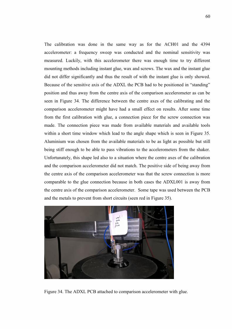
60
The calibration was done in the same way as for the ACH01 and the 4394
accelerometer: a frequency sweep was conducted and the nominal sensitivity was
measured. Luckily, with this accelerometer there was enough time to try different
mounting methods including instant glue, wax and screws. The wax and the instant glue
did not differ significantly and thus the result of with the instant glue is only showed.
Because of the sensitive axis of the ADXL the PCB had to be positioned in “standing”
position and thus away from the centre axis of the comparison accelerometer as can be
seen in Figure 34. The difference between the centre axes of the calibrating and the
comparison accelerometer might have had a small effect on results. After some time
from the first calibration with glue, a connection piece for the screw connection was
made. The connection piece was made from available materials and available tools
within a short time window which lead to the angle shape which is seen in Figure 35.
Aluminium was chosen from the available materials to be as light as possible but still
being stiff enough to be able to pass vibrations to the accelerometers from the shaker.
Unfortunately, this shape led also to a situation where the centre axes of the calibration
and the comparison accelerometer did not match. The positive side of being away from
the centre axis of the comparison accelerometer was that the screw connection is more
comparable to the glue connection because in both cases the ADXL001 is away from
the centre axis of the comparison accelerometer. Some tape was used between the PCB
and the metals to prevent from short circuits (seen red in Figure 35).
Figure 34. The ADXL PCB attached to comparison accelerometer with glue.

61
Figure 35. The ADXL PCB attached to the comparison accelerometer with screws.
When looking at the results in Figure 36 and in Figure 37 it is possible to see that the
ADXL001 is acting quite in a stable way below 1000 Hz with the glue connection and
in even more stable way with the screw connection. It could be said that the response of
the ADXL001 is better than the response of the Brüel & Kjær 4394 below the frequency
of 1000 Hz. The screw connection did not bring stableness to the high frequencies as
was expected. The result in Figure 36 can be easily compared with the equal figure of
the datasheet because they both have scaling in decibels and it can be seen that they are
not similar (Analog Devices 2016e). Below 1000 Hz the results are similar with the
datasheet but for higher frequencies, the test results do not follow a similar flat line as is
shown in the datasheet, instead there are some instabilities. Again, there are multiple
options why the figures do not match: the datasheet might have false information, this
particular ADXL001 is faulty, the used printed circuit is faulty and/or the calibration has
been done in a wrong way.

62
The used printed circuit board with its components might have a natural frequency
somewhere between 1000 Hz and 10 000 Hz which affects to the sensitivity. Another
option is that the given PCB does not have the circuitry/notch filter build in a proper
way. The third option regarding to the influences caused by the PCB could be that the
PCB does not pass the vibration well enough to the ADXL001 accelerometer. The
Analog Devices sell the ADXL001 also connected to a PCB as seen in Figure 17. With
Analog Devices’ own PCB the results might be different.
There might have been also faults in the way the calibration process was carried out and
especially in the mounting between the ADXL001 and the comparison accelerometer.
As said before the axes did not match but also the tightness of screws and the used tape
might have been a problem. Maybe the screws were not tightened enough because of
the fear of breaking the PCB or the insulator tape had some small effect also to the
tightness of the screws and the passing of vibration to the ADXL001. However, with
these results it easy to say that the ADXL001 has a good frequency response below
1000 Hz and could be used for vibration monitoring up to that frequency.
Figure 36. The ADXL001 calibration, installed with glue, ±5 % limits.

63
Figure 37. The ADXL001 calibration, installed with screws, ±5 % limits.
Figure 38. The ADXL001 calibration, installed with screws, ±15 dB limits.
5.2 Raspberry Pi 3 as a sensor platform
The Raspberry Pi3 model B was chosen as a sensor platform because it has reasonable
price, good performance according to the specifications, Wi-Fi and Bluetooth for
wireless communication enabling the possibility to be part of Internet of Things. The
capability of being part of Internet of Things might be actually a big advantage because
it is predicted that by 2020 there will be 50 billion Internet of Things devices (Evans
2011, p.3). Maybe, still the biggest driving factor towards to Raspberry was the large
community of users. The Raspberry forum itself (https://www.raspberrypi.org/forums/)
has 1 039 887 posts, 152 288 topics and 186 136 members (checked at 25.11.2016) but

64
on top of that there are also other forums like the http://raspberrypi.stackexchange.com/.
Also Arduino has a large user community which is revealed by the
https://forum.arduino.cc/: 2 920 708 posts, 370 132 topics and 296 315 members
(checked at 25.11.2016). The reason why Raspberry was chosen before Arduino was
that the Raspberry Pi 3 has much more processing power than any of the Arduinos and
that the processing power could be very useful in signal processing, data storing and
sending data for further manipulation.
Even though the huge community is a big blessing, it is also a bit of a curse. Often there
is not any verified information available (manuals, datasheets, guides etc.) and all the
needed information has to be gathered from different forums. The forum post goodness
has to be weighted somehow and the wanted information needs to be separated from the
unnecessary and the false information. In addition, the writers of these forums might not
have the best writing skills, language skills, correct terms or a unified way to express
their answers/questions and thus it might be quite time consuming to find useful
information. Because the Raspberry is so community based, many of the following
references regarding to the Raspberry are from the Raspberry forums or from some
websites and thus these references are, unfortunately, not so highly appreciated in the
scientific world.
At first, before the Raspberry was purchased, it was roughly checked that the Raspberry
would be able to reach the wanted sample rate when used for data acquisition. It was
possible to find information that the previous Raspberry model has been used even as an
oscilloscope to reach sample rates up to 10 mega samples per second (Pelikan 2014).
This gave promising thoughts for the future and gave the courage to buy the Raspberry
and to start further investigation.
5.2.1 Communication between Raspberry and external hardware
The Raspberry Pi 3 has 40 general-purpose input-output (GPIO) pins and multiple ways
to communicate with external hardware like an ADC (MagPi 2016). The Raspberry Pi
has numerous serial interfaces such as the universal asynchronous receiver/transmitter
(UART), the serial peripheral interface (SPI), the inter-integrated circuit (I2C) and the

65
inter-IC Sound (I2S) (Raspberry Pi Foundation 2016a). The parallel interface is also one
way to communicate between the Raspberry and the external hardware. The SPI and the
parallel interfaces were chosen for further investigation because of their wide usage in
ADC to Raspberry connections and their high speed rates: the maximum speed of SPI is
8 megabits per second (Mbps) and in parallel mode it is possible to use it as an
oscilloscope (10 mega samples per second) (Pelikan 2014, Abyz 2016a, Wootton 2016,
p.335). Even though the SPI information page of the Raspberry Pi Foundation claims
that the SPI has the maximum speed of 125 Mbps it is not reachable anymore when the
signals reach the GPIO pins (Raspberry Pi Foundation 2016d, Raspberry Pi Foundation
- Forum 2016e). The I2C is also widely used in projects that use the Raspberry Pi and
the ADC but it has the maximum speed of 400 kilobits per second (kbps) and thus it is
slower than the parallel interface or the SPI. The I2S might also have use in condition
monitoring applications. The I2S is normally used in audio applications and it is able to
reach a sample rate of ~200 kilo samples per second with the resolution of 24-bit when
operating with the Raspberry Pi (Raspberry Pi Foundation - Forum 2016b).
The SPI was originally developed by Motorola but nowadays it is a bit loosely defined
(McGrath, Scanaill 2013, p.63). Usually the SPI needs 4 wires to work: the slave select
(SS) line to choose one of connected peripherals, the master-out slave-in (MOSI) to
send data from the master device (for example CPU) to the slave device (for example
ADC), the master-in slave-out (MISO) to receive data from the slave and the clock
signal line (SCLK) to give the clock signal to the slave and to control the data stream
(Wootton 2016, pp.335-336, McGrath, Scanaill 2013, p.63). The SPI works in full
duplex mode meaning that the data is sent to the slave and received from the slave
simultaneously (McGrath, Scanaill 2013, p.63). The data stream is controlled by the
master device.
The parallel interface allows sending multiple bits at once but it also needs as many
wires as it has bits to send and in addition a clock wire (Pelikan 2014, p.8). As described
earlier, the parallel interface can reach even the speed of 10 mega samples per second
with the Raspberry but there is also a problem: the system interrupts are disabled and
thus sampling in this manner can be performed only for a millisecond or so without
causing any interrupt related problems to the Linux operating system (Pelikan 2014,

66
p.6). When the investigation of using the Raspberry as a sensor platform was carried, it
was hoped that the parallel interface could also be an option for longer sampling times
when the sample rate was slightly reduced.
5.2.2 Programming Raspberry
The Raspberry has a couple of text-editors (some have also features like colouring to
make the programming easier) installed in advance that can be used for programming:
Leafpad, IDLE, Nano and VI (Raspberry Pi Foundation 2016e). In addition, there are
more text editors and integrated development environments (IDEs) that can be
downloaded afterwards. For fast software applications, like fast ADC sampling, the
programming language C is usually recommended over Python and that is the reason
why it was chosen for this project (Raspberry Pi Foundation - Forum 2016f, Raspberry
Pi Foundation - Forum 2016d, Raspberry Pi Foundation - Forum 2016c, Raspberry Pi
Foundation - Forum 2016a). There are popular libraries to access the GPIOs of the
Raspberry through the programming language C like PIGPIO, Wiring Pi and Mike
McCauley’s one (Abyz 2016b, Henderson 2016, McCauley 2016). The PIGPIO library
was chosen for this project because Abyz seems to be an active member in the
Raspberry Pi forums and is willing to help when problems occur.
5.2.3 Raspberry & EVAL-AD7609
The EVAL-AD7609 from Analog devices was chosen as the analogue interface because
of its good features. The ADC used in the EVAL-AD7609 is the AD7609 having the
same features as the AD7608 described in chapter 8.2 Measurement system from
integrated circuits added on the evaluation board which provides better access to the
ADCs pins and an extra reference voltage. Without any previous programming or
electronics background, it turned out to be quite time consuming and difficult to get the
EVAL-AD7609 and the Raspberry to work together. Unfortunately, the time reserved
for this thesis ended before this connection could be made to work properly.
The EVAL-AD7609 has the SPI and the parallel interfaces. The parallel interface was
chosen at first after seeing the Raspberry used as an oscilloscope in the Pelikan’s project
and because of the basic concept of the parallel interface’s capability to transfer

67
multiple bits at once. The capability of the PIGPIO to read the GPIOs just every 5
microsecond leads to the maximum reading rate of 200 000 reads per second. The
EVAL-AD7609 has 8 channels and a parallel interface that has to send bits in two
sections per channel which leads to a sample rate of (200 000 sps / 8) / 2 = 12 500 sps.
The poor performance of the parallel interface with the PIGPIO led to the change of the
angle of the approach to use the SPI instead.
Ambitiously an option was searched to get all the power into use from the EVAL-
AD7609 but unfortunately after long hours spent with the Raspberry and learning about
the SPI, the PIGPIO, programming, and electronics a working solution was not found.
Even though the SPI’s maximum speed of 8 MHz is presented earlier in this thesis, it
was not found in the early stage of attempts. The EVAL-AD7609 needs the SPI clock
speed of 20 MHz to work in full speed and with 8 MHz SPI clock the full speed was not
reached in this thesis. The clock signals of 1 MHz, 4 MHz, 8 MHz, 16 MHz, 31 MHz
and 63 MHz are shown in Figure 40 - Figure 45 and it can be seen that the step like
signal is transforming towards a sinusoidal signal when the frequency increases. The
arrangements for the oscilloscope measurements can be seen in Figure 39.
With more time and with wider knowledge about programming and electronics,
solutions to get the Raspberry Pi and the EVAL-AD7609 combination to work might be
found. Also, the fact that the Raspberry Pi has been used successfully as an oscilloscope
gives hope of success. The solution for this problem might be found from better
programming or using the Raspberry without any operating system in a so-called bear
metal mode.
Figure 39. Arrangements for oscilloscope measurements with the Raspberry Pi.

68
Figure 40. 1 MHz hardware clock signal from the Raspberry Pi.
Figure 41. 4 MHz hardware clock signal from the Raspberry Pi.
Figure 42. ~ 8 MHz hardware clock signal from the Raspberry Pi.

69
Figure 43. ~ 16 MHz hardware clock signal from the Raspberry Pi.
Figure 44. ~ 31 MHz hardware clock signal from the Raspberry Pi.
Figure 45. ~ 63 MHz hardware clock signal from the Raspberry Pi.

70
6 DISCUSSION
The budget of 100 € is too low for a complete vibration monitoring system that is
capable to do bearing monitoring up to 10 000 Hz signals and to have 16-bit resolution.
The only thinkable solution under 100 € was the system built from ICs. The IC
component prices are well suited to the wanted limit of 100 € and the specifications of
those components are also more than suitable to meet the criteria of being able to
measure signals up to 10 000 Hz with the resolution of 16-bit. With 100 € it is possible
to get a 24-bit ADC, with sample rate over 100 ksps, high order anti-aliasing filter,
amplification, processor and even an accelerometer like ADXL001. The problem comes
when these ICs are connected together: the programming, electronic circuit designing
and connecting the electronic components might be time consuming (time is money). In
addition, sometimes expensive tools maybe needed (like good soldering iron for small
ICs) and electrical and programming knowledge should be high enough to be able to
design non-noisy circuits and have effective and fast code which is able to sample fast
enough and to do data manipulation. Luckily new ICs are coming that integrate many of
the data-acquisition components to one chip like the AD7608 which has reference
voltage, track-and-hold amplifiers, anti-alias filter and digital filter all integrated to one
chip. The integration of the chips loosens the requirements for the needed wide
knowledge about electronics and noise cancellation because many of the connections
between components have already been taken care by the manufacturer.
Promising low-cost accelerometers were also found or at least promising specifications
of accelerometers like the ACH 01 from Te Connectivity and the ADXL001 from
Analog Devices. When these promising accelerometers were tested, the sensitivity of
vibration monitoring was revealed. The ACH 01 did not follow at all its specification
but with the ADXL001 the results were promising up to 1000 Hz. Most likely, it is
possible to find the full potential of the ADXL001 in right conditions where the
sensitivity of vibration monitoring is taken even more seriously: if the ADXL001 is
connected to a PCB, the PCB has to be able to pass the vibration without affecting to it
(for example the resonance frequency should be high enough for the PCB and it should
not damp the vibration) and the connection of the ADXL001 or the ADXL001 and the
71
PCB to the measuring location should be made stiff enough and to an optimal point (the
screw connection is usually the best and the accelerometer should be as near as possible
to the measurement location without having any extra barriers in between). The few
euro accelerometers were not able to reach the 10 000 Hz goal but they might be useful
in other condition monitoring applications with lower frequencies. Though it have to be
noted that many of the digital MEMS do not have an anti-aliasing filter build in. The
lack of anti-aliasing filter has to be taken care of for example by using mechanical
filters. Because of the low bandwidth they are not capable to measure defects from
small bearings but might be usable with big bearings as the equation (1) shows.
The smart sensors form a class of their own when compact designs are needed or when
multiple physical phenomena must be measured from the same location. Depending on
the smart sensor, they can have many features included: multiple sensors in a single
package, local data processing, wireless connection and so on. The Internet of Things is
raising a lot of interest nowadays and the smart sensors with their wireless
communication and local data processing are almost like made for IoT. The local data
processing of a sensor minimises the amount of data transferred and reduces the needed
storage space in the receiver device. The smart sensors with many features can be
reasonable priced but when a smart sensor for bearing condition monitoring is wanted;
the cost rises to hundreds of euros per accelerometer. The ADIS16227 is a good
example of a smart sensor which is designed for vibration monitoring.
There are plenty of USB DAQs/oscilloscopes and ADC evaluation boards available for
vibration monitoring up to 10 kHz but unfortunately, they are a bit too pricy as the price
does not stay under 100 €. Under 200 € with the accelerometer and the processing unit
might be feasible and also with the acceptable specifications reaching even 18-bit
resolution, 200 ksps per second sample rate per channel and 8 channels if for example
the EVAL-AD7609 is used. If easier connectivity is needed and a computer is available
for data acquisition then the USB DAQ/oscilloscope might be the way to go. There are a
wide variety of USB data acquisition devices available with varying features and costs.
There are inexpensive and slow DAQ devices and also high end devices which cost
thousands of euros. Often the USB DAQ/oscilloscope gets the electrical power from the
USB port making them portable devices when connected for example to a laptop.

72
Unfortunately, the test of the Raspberry Pi 3 being used as a sensor platform and signal
processing device with the EVAL-AD7609 did not work out in the time window
reserved for the thesis. There is still hope that the Raspberry Pi 3 might work in high
speed data acquisition. In the right hands, with more time and maybe with some external
hardware it might be possible to get it working. There are also plenty of other single-
board computers and microcontrollers that possibly could be used instead of the
Raspberry Pi when sensor platform or processing unit is searched.

73
7 SUMMARY
An overall overview of data acquisition components for vibration based condition
monitoring was carried out in this thesis. The different accelerometer types available
including MEMS, piezofilm and piezoelectric accelerometers were studied. The
importance of amplification and filtering were simulated: the amplification has an effect
to the resolution of the sampled signal and with the filtering it is possible to avoid
aliasing. The ADCs resolutions effect on the gathered data was also shown with
simulation. Technical discussion of data vibration monitoring components has been
carried out component by component: accelerometers, amplifiers, filters, ADCs and
processors were covered. Consequently the third research question "What kind of
parameters do individual measurement device components have and what kind of
meaning do they have related to the gathered vibration signal data?" has been covered
quite well.
Unfortunately, no complete low-cost system for bearing vibration monitoring costing
under 100 € was found and thus this thesis does not offer any straight forward solution
for low-cost bearing monitoring. Many different devices were studied but most likely
there are still more devices to check out which leads to a suggestion for future work:
even a wider market review could be possible. Also, the testing of other low-cost
devices than tested in this thesis should be done due to the contradicting results between
the specification sheets and the test results showed in the accelerometer testing. One
thing that has to be noted is that the cheapest is not always the easiest option. In
addition, the development time, which is used to make the cheap option to work, should
be valued. Also, there might not be huge interest in companies to build their own
devices for condition monitoring.
Technology is developing all the time which lowers the prices and that is the case with
accelerometers also. With nowadays accelerometers costing less than 10 euros it might
be already possible to do condition monitoring for large bearings but in the future it
might be more of a rule than exception that bearings of all sizes are measured with the
low-cost accelerometers. A suggestion for further work is to test these shown and
upcoming low-cost accelerometers in real world applications.

74
8 REFERENCES
ABYZ, J., 2016a. Frequently Asked Questions - PIGPIO [online]. Available:
http://abyz.co.uk/rpi/pigpio/faq.html [11/26, 2016].
ABYZ, J., 2016b. PIGPIO [online]. Available: http://abyz.co.uk/rpi/pigpio/index.html
[11/27, 2016].
AGOSTON, K., 2012. ACCELEROMETER CHARACTERISTICS, ERRORS AND
SIGNAL CONDITIONING. The International Conference Interdisciplinarity in
Engineering, January 2012, “Petru Maior” University of Tîrgu Mureş Romania, pp.
276-281.
ANALOG DEVICES, 2016a. AD7608 specification [online]. Available:
http://www.analog.com/media/en/technical-documentation/data-sheets/AD7608.pdf
[11/25, 2016].
ANALOG DEVICES, 2016b. ADIS16223 Overview [online]. Available:
http://www.analog.com/en/products/mems/accelerometers-special-
purpose/adis16223.html#product-overview [11/10, 2016].
ANALOG DEVICES, 2016c. ADIS16227 Overview [online]. Available:
http://www.analog.com/en/products/mems/accelerometers-special-
purpose/adis16227.html#product-overview [11/10, 2016].
ANALOG DEVICES, 2016d. ADXL001 Specifications [online]. Available:
http://www.analog.com/media/en/technical-documentation/data-sheets/ADXL001.pdf
[11/7, 2016].
ANALOG DEVICES, 2016e. CN-0303 Specifications [online]. Available:
http://www.analog.com/media/en/reference-design-documentation/reference-
designs/CN0303.pdf [11/7, 2016].
ANALOG DEVICES, 2016f. EVAL-AD7608 - Specifications [online]. Available:
http://www.analog.com/en/design-center/evaluation-hardware-and-software/evaluation-
boards-kits/EVAL-AD7608.html#eb-overview [11/27, 2016].
ARCHIEM, 2016. Piezoelectric Accelerometer - Figure [online]. Available:
https://en.wikipedia.org/wiki/File:PiezoAccel.jpg [12/1, 2016].
ARDUINO, 2016. What is Arduino [online]. Available:
http://www.arduino.org/learning/getting-started/what-is-arduino [11/14, 2016].
BENGTSSON, M., 2004. CONDITION BASED MAINTENANCE SYSTEMS – AN
INVESTIGATION OF TECHNICAL CONSTITUENTS AND ORGANIZATIONAL
ASPECTS. Licentiate Mälardalen University.

75
BROCH, J.T. ,1980. Mechanical vibration and shock measurements. Copenhagen:
Bruel & Kjaer. 370 p. ISBN 878-73553-6-1.
DAMATO, A., 2016. Low-pass filters - Figure [online]. Available:
https://commons.wikimedia.org/wiki/File:Electronic_linear_filters.svg [12/1, 2016].
DATA PHYSICS, 2016. Quattro [online]. Available:
http://www.dataphysics.com/products-and-solutions/dynamic-signal-analyzers-
signalcalc/signalcalc-ace.html [11/29, 2016].
DIAGNOSTIC SOLUTIONS, 2016. USB-Vib Portable Vibration Meter [online].
Available: http://diagsol.co.uk/products/usb-portable-vibration-meter/ [11/29, 2016].
DIAGNOSTIC SOLUTIONS, USB Vib Sensor – Specification Sheet [online].
Available: http://diagsol.co.uk/wp-content/uploads/2010/06/usb-vib-spec-sheet.pdf
[11/29, 2016].
DIGIDUCER INC., 2016a. 333D01 Overview [online]. Available: http://digiducer.com/
[11/10, 2016].
DIGIDUCER INC., 2016b. 333D01 Specifications [online]. Available:
http://digiducer.com/pages/specifications [11/10, 2016].
DOSCHER, J., 2016. Accelerometer Design and Applications [online]. Available:
http://elpuig.xeill.net/Members/vcarceler/articulos/jugando-con-el-wiimote-y-gnu-
linux/sensor971.pdf/at_download/file [11/13, 2016].
EL-THALJI, I., 2016. Dynamic modelling and fault analysis of wear evolution in
rolling bearings. Espoo: VTT Technical Research Centre of Finland Ltd. ISBN 978-
951-38-8416-1.
EVANS, D., 2011. The Internet of Things How the Next Evolution of the Internet Is
Changing Everything. Cisco Internet Business Solutions Group (IBSG).
FRANK, R. ,2013. Understanding Smart Sensors. Norwood: Artech House. ISBN 978-
160-80750-8-9.
GATTI, P.L. and FERRARI, V. ,2002. Applied Structural and Mechanical Vibrations :
Theory, Methods and Measuring Instrumentation (2). London: CRC Press. ISBN 978-
020-30145-5-4.
GAURA, E. and NEWMAN, R. ,2006. Smart Mems and Sensor Systems. London: ICP.
ISBN 978-186-09492-0-3.
GIACHINO, J.M., 1986. Smart sensors. Sensors and Actuators, Vol. 10, No. 3-4, pp.
239-248.

76
HENDERSON, G., 2016. Wiring Pi [online]. Available: http://wiringpi.com/ [11/27,
2016].
HOLMBERG, K., ADGAR, A., JANTUNEN, E., MASCOLO, J., ARNAIZ, A. and
MEKID, S. ,2010. E-maintenance. 511 p. ISBN 978-1-84996-204-9.
HUIJSING, J.H. ,2008. Smart Sensor Systems: Why? Where? How? ISBN 978-047-
08669-3-1.
IEEE, 1998. IEEE Standard for a Smart Transducer Interface for Sensors and Actuators
- Transducer to Microprocessor Communication Protocols and Transducer Electronic
Data Sheet (TEDS) Formats.
INVENSENSE, 2016. MPU-9250 Specification [online]. Available:
https://www.invensense.com/products/motion-tracking/9-axis/mpu-9250/ [11/10, 2016].
J. JOHANSSON, P. E. MARTINSSON and J. DELSING, 2007. Simulation of Absolute
Amplitudes of Ultrasound Signals Using Equivalent Circuits. IEEE transactions on
ultrasonics, ferroelectrics, and frequency control, Vol. 54, No. 10, pp. 1977-1983. ISSN
0885-3010.
KIONIX, 2016. KX122-1037 Specifications [online]. Available:
http://kionixfs.kionix.com/en/datasheet/KX122-1037 Specifications Rev 5.0.pdf [11/6,
2016].
LI, C., LIANG, M. and WANG, T., 2015. Criterion fusion for spectral segmentation and
its application to optimal demodulation of bearing vibration signals. Mechanical
Systems and Signal Processing, Vol. 64–65, pp. 132-148. ISSN 0888-3270.
LINEAR TECHNOLOGY, 2016. Linear Tehcnology Home page [online]. Available:
http://www.linear.com/ [11/29, 2016].
MAGPI, 2016. RASPBERRY PI 3 IS OUT NOW! SPECS, BENCHMARKS & MORE
[online]. Available: https://www.raspberrypi.org/magpi/raspberry-pi-3-specs-
benchmarks/ [11/26, 2016].
MÄKELÄ, M. ,2008. Tekniikan kaavasto : matematiikan, fysiikan, kemian ja
lujuusopin peruskaavoja sekä SI-järjestelmä. 10 edn. Tampere: Tammertekniikka. 208
p. ISBN 978-952-5491-48-7.
MAXIM INTEGRATED, 2016a. Glossary Definition For Analog-Front-End [online].
Available: https://www.maximintegrated.com/en/glossary/definitions.mvp/term/Analog-
Front-End/gpk/11 [11/22, 2016].
MAXIM INTEGRATED, 2016b. MAX7427 Specifications [online]. Available:
https://datasheets.maximintegrated.com/en/ds/MAX7426-MAX7427.pdf [11/7, 2016].
77
MCCAULEY, M., 2016. C library for Broadcom BCM 2835 [online]. Available:
http://www.airspayce.com/mikem/bcm2835/index.html [11/27, 2016].
MCGRATH, M.J. and SCANAILL, C.N. ,2013. Sensor technologies: Healthcare,
wellness, and environmental applications. 302 p. ISBN 978-143026014-1.
MEASUREMENT COMPUTING CORP. ,2012. Data Acquisition Handbook. 3 edn.
Norton: Measurement Computing corp.
MEASUREMENT SPECIALTIES., 1999. Piezo Film Sensors Technical Manual.
Norristown: Measurement Specialties.
MICROCHIP, 2016. MCP6S21 Specifications [online]. Available:
http://ww1.microchip.com/downloads/en/DeviceDoc/21117B.pdf [11/7, 2016].
MIETTINEN, J., LEINONEN, P., JANTUNEN, E., KOKKO, V., RIUTTA, E., SULO,
P., KOMONEN, K., LUMME, V.E., KAUTTO, J., HEINONEN, K., LAKKA, S.,
MÄKELÄINEN, R. and MIKKONEN, H. ,2009. Kuntoon perustuva kunnossapito :
käsikirja. Helsinki: KP-Media. 606 p. ISBN 978-952-99458-4-9.
NOHYNEK, P. and LUMME, V.E. ,2004. Kunnonvalvonnan värähtelymittaukset. 2
edn. Rajamäki: KP-Media. 146 p. ISBN 951-97101-9-1.
PELIKAN, D., 2014. Building an oscilloscope with a Raspberry Pi. The MagPi; A
Magazine for Raspberry Pi Users, Vol. 24, pp. 4-9.
RASPBERRY PI FOUNDATION, 2016a. Frequently Asked Questions [online].
Available: https://www.raspberrypi.org/help/faqs/ [11/26, 2016].
RASPBERRY PI FOUNDATION, 2016b. Raspberry Pi Foundation Strategy [online].
Available:
https://www.raspberrypi.org/files/about/RaspberryPiFoundationStrategy2016-18.pdf
[11/14, 2016].
RASPBERRY PI FOUNDATION, 2016c. Raspberry Pi homepage [online]. Available:
https://www.raspberrypi.org/ [11/14, 2016].
RASPBERRY PI FOUNDATION, 2016d. SPI - Raspberry Pi Documentation [online].
Available:
https://www.raspberrypi.org/documentation/hardware/raspberrypi/spi/README.md
[11/26, 2016].
RASPBERRY PI FOUNDATION, 2016e. Text Editors [online]. Available:
https://www.raspberrypi.org/documentation/linux/usage/text-editors.md [11/27, 2016].
RASPBERRY PI FOUNDATION - FORUM, 2016a. Accessing GPIO which is
fastest?[online]. Available:

78
https://www.raspberrypi.org/forums/viewtopic.php?f=63&t=36784&p=307571&hilit=i
nterrupt+fastest#p307571 [11/27, 2016].
RASPBERRY PI FOUNDATION - FORUM, 2016b. Can Raspberry read multiple
Analog Inputs?[online]. Available:
https://www.raspberrypi.org/forums/viewtopic.php?f=91&t=83830&p=593164&hilit=C
an+Raspberry+read+multiple+Analog+Inputs+%3F#p593164 [11/26, 2016].
RASPBERRY PI FOUNDATION - FORUM, 2016c. Faster SPI [online]. Available:
https://www.raspberrypi.org/forums/viewtopic.php?t=84159&p=596914 [11/27, 2016].
RASPBERRY PI FOUNDATION - FORUM, 2016d. High speed detection [online].
Available: https://www.raspberrypi.org/forums/viewtopic.php?f=37&t=155381 [11/27,
2016].
RASPBERRY PI FOUNDATION - FORUM, 2016e. RPI Compute SPI Signal Problem
[online]. Available:
https://www.raspberrypi.org/forums/viewtopic.php?f=33&t=137817&p=916984&hilit=
pigpio+spi+adc#p916984 [11/26, 2016].
RASPBERRY PI FOUNDATION - FORUM, 2016f. Storing GPIO data in a file in Pi
[online]. Available:
https://www.raspberrypi.org/forums/viewtopic.php?f=91&t=131473&p=877504&hilit=
pigpio+interrupt+latenc%2A#p877504 [11/27, 2016].
RUUVITAG, 2016. RuuviTag Specifications [online]. Available: http://ruuvitag.com/
[11/10/2016, 2016].
SAFIZADEH, M.S. and LATIFI, S.K., 2014. Using multi-sensor data fusion for
vibration fault diagnosis of rolling element bearings by accelerometer and load cell.
Information Fusion, Vol. 18, pp. 1-8. ISSN 1566-2535.
SASSI, S., BADRI, B. and THOMAS, M., 2007. A Numerical Model to Predict
Damaged Bearing Vibrations. Journal of Vibration and Control, Vol. 13, No. 11, pp.
1603-1628. ISSN 1077-5463.
SCHMARTBOARD, 2016. Active Filter Board - Specifications [online]. Available:
http://schmartboard.com/content/Other/MFB%20Application_9.pdf [11/29, 2016].
SHAHZAD, K., CHENG, P. and OELMANN, B., 2013. Architecture exploration for a
high-performance and low-power wireless vibration analyzer. IEEE Sensors Journal,
Vol. 13, No. 2, pp. 670-682.
STMICROELECTRONICS, 2016a. LIS2DH Specification [online]. Available:
http://www.st.com/content/ccc/resource/technical/document/datasheet/c1/e1/62/31/d2/b
1/4d/bb/DM00042751.pdf/files/DM00042751.pdf/jcr:content/translations/en.DM00042
751.pdf [11/6, 2016].

79
STMICROELECTRONICS, 2016b. LIS2DH12 Specifications [online]. Available:
http://www.st.com/content/ccc/resource/technical/document/datasheet/12/c0/5c/36/b9/5
8/46/f2/DM00091513.pdf/files/DM00091513.pdf/jcr:content/translations/en.DM000915
13.pdf [11/10, 2016].
STMICROELECTRONICS, 2016c. LIS2DS12 Specifications [online]. Available:
http://www.st.com/content/ccc/resource/technical/document/datasheet/ce/32/55/ac/e1/87
/46/84/DM00177048.pdf/files/DM00177048.pdf/jcr:content/translations/en.DM001770
48.pdf [11/6, 2016].
TANDON, N. and CHOUDHURY, A., 1999. A review of vibration and acoustic
measurement methods for the detection of defects in rolling element bearings. Tribology
International, Vol. 32, No. 8, pp. 469-480. ISSN 0301-679X.
TE CONNECTIVITY, 2016. ACH 01 Specifications [online]. Available:
http://www.te.com/usa-en/product-CAT-PFS0014.html [11/7, 2016].
TEQUIPMENT, 2017. Distributor of major brands of test equipment [online].
Available: http://www.tequipment.net/ [03/03, 2017].
TEXAS INSTRUMENTS, 2016. SensorTag Specifications [online]. Available:
http://www.ti.com/ww/en/wireless_connectivity/sensortag2015/ [11/10, 2016].
URBAN, G., 2016. Jacob Fraden: Handbook of modern sensors: physics, designs, and
applications. Analytical and bioanalytical chemistry, Vol. 408, No. 21, pp. 5667-5668.
WILSON, J.S. ,2005. Sensor Technology Handbook. Amsterdam: Newnes. ISBN 978-
075-06772-9-5.
WOOTTON, C. ,2016. Beginning Samsung ARTIK: a guide for developers. East
Sussex: Apress. ISBN 978-1-4842-1951-5.
ZARATE, E., 2016. Digital Data Acquisition System - Figure [online]. Available:
https://en.wikipedia.org/wiki/File:DigitalDAQv2.pdf [12/1, 2016].

Appendix 1. Mathcad Prime 3 model of shock signal & ADC.

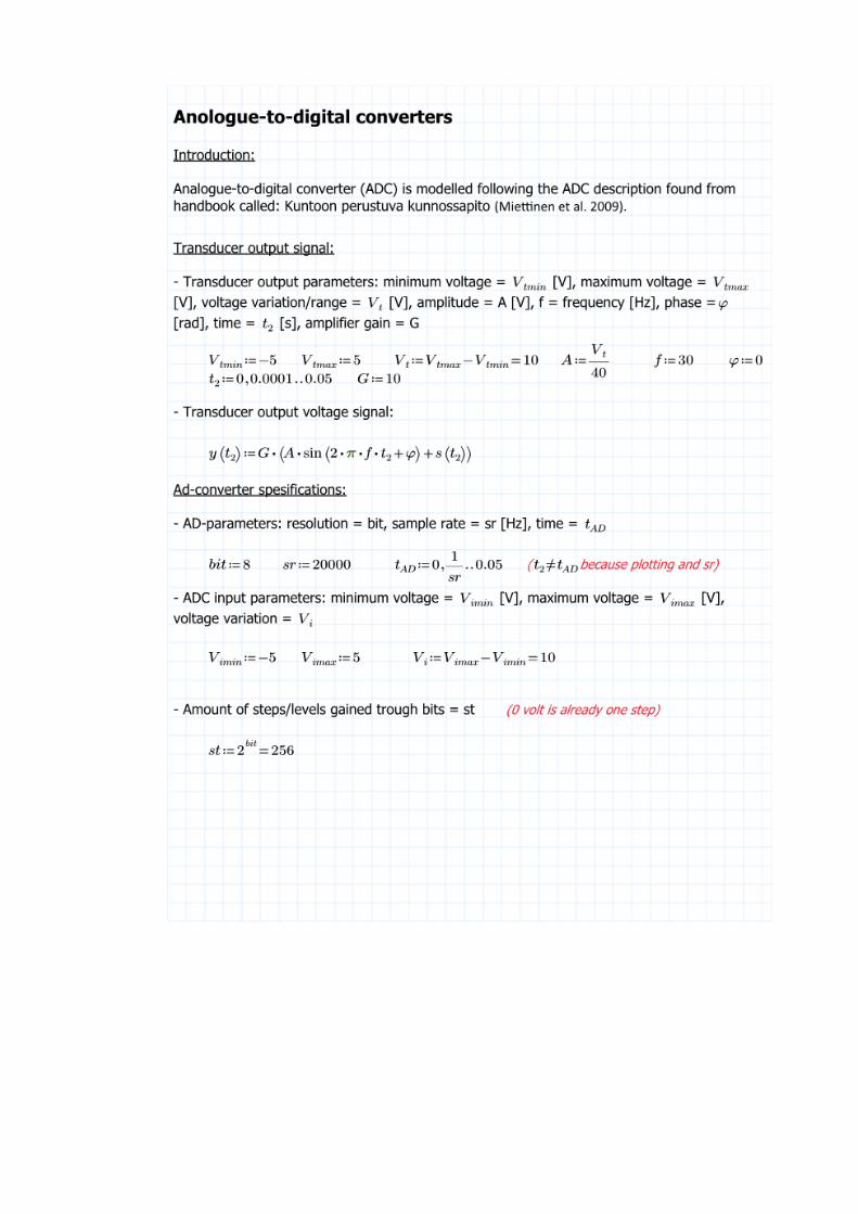


Appendix 2. Basics of a signal path and processing modelled with Mathcad Prime 3.


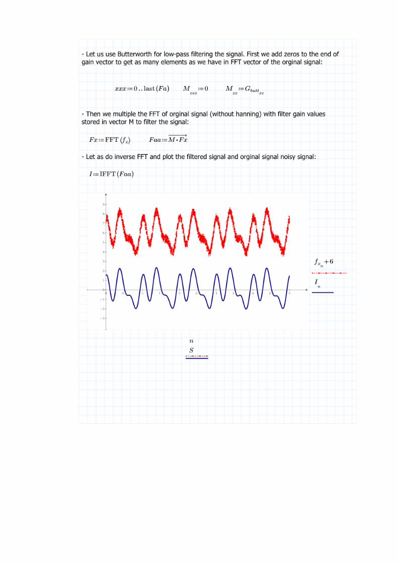

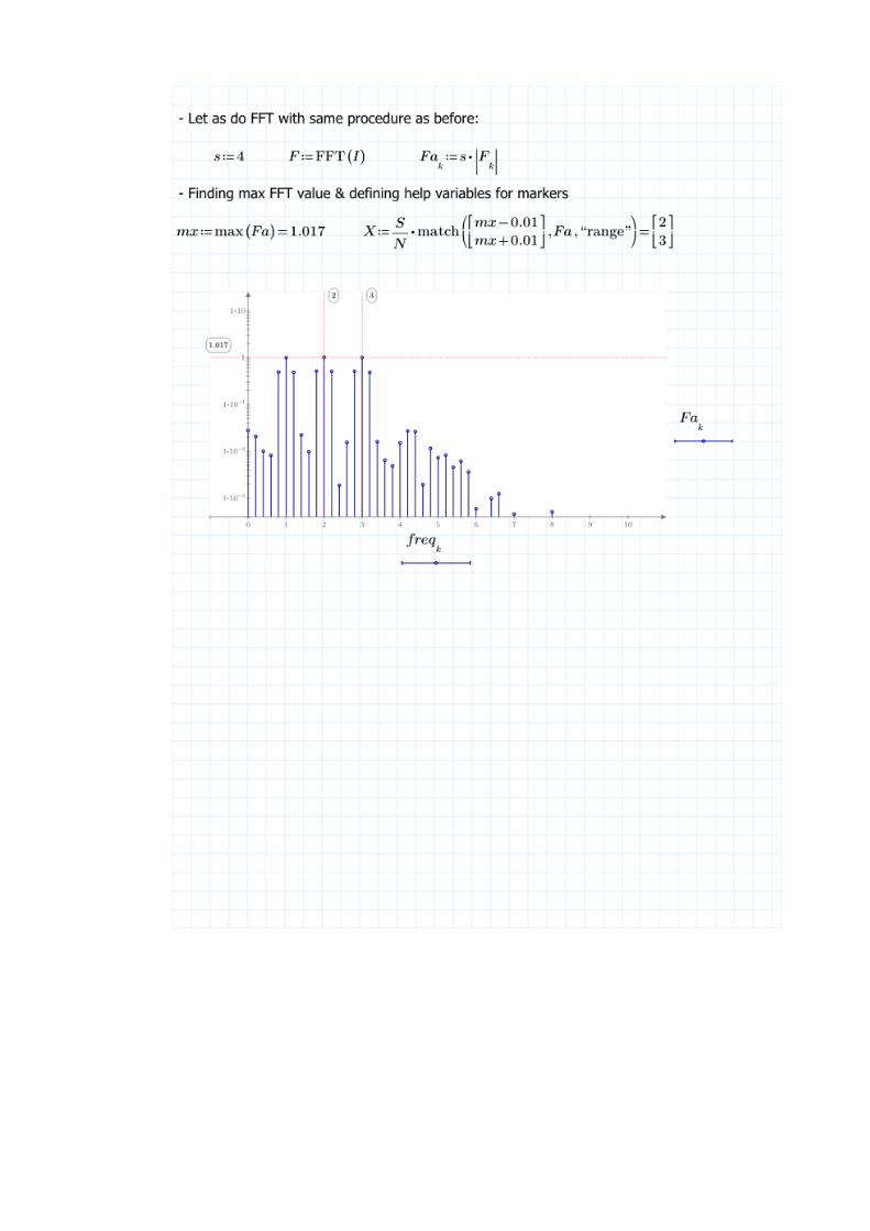

Appendix 3. Accelerometers.
Accelerometers
Man
ufa
ctu
rer
Mo
de
l
Typ
e
Fre
qu
en
cy
BW
(H
z)
Re
son
ant
Fre
qu
en
cy
(Hz)
Am
plit
ud
e
ran
ge (
± g)
Re
solu
tio
n
(bit
)
No
tes
Pri
ce (
abo
ut)
Analog Devices ADIS16227 Digital 14250 22000 1, 5, 20, 70 16
Measures in three direction, has signal
processing in it (FFT [512 point], alarms, averaging
[up to 256]), digital temperature and power
supply measurement. Cost with board 340 €.
250,00 €
Analog Devices ADXL001 Analogue 22000 22000 70 / 250 /
500
Electromechanical self-test, Evaluation board also available without soldering needs (77 €)
28,00 €
TE connectivity ACH-01 Analogue 20000 35000 150
Made out of piezoelectric polymer film.
54,00 €
Kionix KX122-1037 Digital 800 3500 2, 4, 8 16 Triaxis, self-test 2,44 €
ST LIS2DS12 Digital ? ? 2, 4, 8, 16 16 Embedded temperature sensor, Self-test, 3-axis
3,28 €
ST MIS2DH Digital ? ? 2, 4, 8, 16 12 Embedded temperature sensor, Self-test, 3-axis
11,28 €
ST LIS2DH Digital ? ? 2, 4, 8, 16 12 Embedded temperature sensor, Self-test, 3-axis.
1,85 €

Appendix 4. ADC ICs.
IC ADC
Manufacturer Model ADC Type
Resolution (bit)
Channels
Max Sample Rate
(Hz)/channel
Integrated Amp max
Gain
Analog Devices AD1871YRSZ ΣΔ 24 2 single-ended or
differential 96000
Analog Devices AD7173-8BCPZ ΣΔ 24 8 differential or 16 single-ended
31250
Analog Devices AD7175-2BRUZ ΣΔ 24 2 differential or 4
single-ended 50000
Analog Devices AD7176-2 ΣΔ 24
2 fully differential or 4 pseudo differential
50000
Analog Devices AD7476 SAR 12 1- single-ended 1000000
Analog Devices AD7606BSTZ SAR 16 8 single-ended 200000
Analog Devices AD7606BSTZ-4 SAR 16 4 single-ended 200000
Analog Devices AD7608 SAR 18 8 single-ended 200000
Analog Devices AD7609 SAR 18 8 differential 200000
Analog Devices AD7711ARZ ΣΔ 24 1 differential and
1 single-ended 19500 128
Analog Devices AD7760BSVZ ΣΔ 24 1 differential 2500000
Analog Devices AD7765BRUZ ΣΔ 24 1 differential 156000
Analog Devices AD7766BRUZ SAR 24 1 differential 128000
Analog Devices AD7767BRUZ-2 SAR 24 1 differential 32000
Analog Devices ADAR7251 ΣΔ 16 4 differential 1800000 45 dB
Texas Instruments ADS1251U ΣΔ 24 1 differential 20000
Texas Instruments ADS1252U ΣΔ 24 1 differential 40000
Texas Instruments ADS1255IDBT ΣΔ 24 1 differential or
two single-ended 30000 64
Texas Instruments ADS1258IRTCTG4 ΣΔ 24 16 single-ended or 8 differential
23700
Texas Instruments ADS1271 ΣΔ 24 1 differential 105000
Texas Instruments ADS1274IPAPT ΣΔ 24 4 differential 144000
Texas Instruments ADS1278IPAPT ΣΔ 24 8 single-ended 144000
Texas Instruments ADS1294IPAG ΣΔ 24 4 differential 32000 12
Texas Instruments ADS131A04 ΣΔ 24 4 differential 128000
Texas Instruments ADS8344 SAR 16 8 single-ended or
4 differential 12500
Texas Instruments PCM1801U ΣΔ 16 1 single-ended 48000
Texas Instruments PCM1803ADB ΣΔ 24 1 Single-ended 96000
Texas Instruments PCM1808PWG4 ΣΔ 24 1 single-ended 96000
Texas Instruments PCM3500EG4 ΣΔ 16 1 single-ended 26000
Texas Instruments PCM4201 ΣΔ 24 1 differential 108000
Texas Instruments PCM4204PAPT ΣΔ 24 4 differential 216000
Texas Instruments PCM4220PFB ΣΔ 24 2 differential 216000
NXP UDA1361TS/N1 ΣΔ 24 1 single-ended 110000

IC ADC
Manufacturer Model Integrated Filter Types
Low-pass Filter Cutoff Frequency -
3dB (Hz)
SNR [dB]
Data Interfaces Price
(about) Data Sheet
Analog Devices AD1871YRSZ digital low-
pass 106
SPI® 9,40 €
http://www.analog.com/media/en/technical-
documentation/data-sheets/AD1871.pdf
Analog Devices AD7173-8BCPZ
?
SPI®; QSPI™; MICROWIRE™; DSP compatible
14,00 €
http://www.analog.com/media/en/technical-
documentation/data-sheets/AD7173-8.pdf
Analog Devices AD7175-2BRUZ
Digital
?
SPI®; QSPI™; MICROWIRE™; DSP compatible
18,68 €
http://www.analog.com/media/en/technical-
documentation/data-sheets/AD7175-2.pdf
Analog Devices AD7176-2
Digital filters (sinc 1, sinc 3,
sinc 5)
?
SPI®; QSPI™; MICROWIRE™; DSP compatible
16,50 €
http://www.analog.com/media/en/technical-
documentation/data-sheets/AD7176-2.pdf
Analog Devices AD7476
70
SPI®; QSPI™; MICROWIRE™; DSP compatible
7,50 €
http://www.analog.com/media/en/technical-
documentation/data-sheets/AD7476_7477_747
8.pdf
Analog Devices AD7606BSTZ
Anti-alias (2nd. Ord.), digital filter
15 000 or 22 000
95.5
SPI®; QSPI™; MICROWIRE™; DSP compatible
25,45 €
http://www.analog.com/media/en/technical-
documentation/data-sheets/AD7606_7606-
6_7606-4.pdf
Analog Devices AD7606BSTZ-4
Anti-alias (2nd. Ord.), digital filter
15 000 or 22 000
95.5
SPI®; QSPI™; MICROWIRE™; DSP compatible
16,95 €
http://www.analog.com/media/en/technical-
documentation/data-sheets/AD7606_7606-
6_7606-4.pdf
Analog Devices AD7608
Anti-alias (2nd. Ord.), digital filter
15 000 or 23 000
90.9
SPI®; QSPI™; MICROWIRE™;
DSP compatible; Parallel
30,65 €
http://www.analog.com/media/en/technical-
documentation/data-sheets/AD7608.pdf
Analog Devices AD7609
Low-pass Filter + Digital
filter
23000 or 32000
91
SPI®; QSPI™; MICROWIRE™;
DSP compatible; Parallel
33,48 €
http://www.analog.com/media/en/technical-
documentation/data-sheets/AD7609.pdf
Analog Devices AD7711ARZ Digital low-pass filter
? Serial 30,19 €
http://www.analog.com/media/en/technical-
documentation/data-sheets/AD7711.pdf
Analog Devices AD7760BSVZ FIR low-pass
112 Parallel 45,49 €
http://www.analog.com/media/en/technical-
documentation/data-sheets/ADAR7251.pdf
Analog Devices AD7765BRUZ FIR low-pass
107 SPI® 17,27 €
http://www.analog.com/media/en/technical-
documentation/data-sheets/AD7765.pdf
Analog Devices AD7766BRUZ FIR low-pass, Digital filter
108.5 Serial 10,80 €
http://www.analog.com/media/en/technical-
documentation/data-sheets/AD7766.pdf
Analog Devices AD7767BRUZ-
2 FIR low-pass
113.5 Serial 14,67 €
http://www.analog.com/media/en/technical-
documentation/data-sheets/AD7767.pdf
Analog Devices ADAR7251
Decimation filters, High-
Pass filter
94 SPI®; Parallel 16,01 €
http://www.analog.com/media/en/technical-
documentation/data-sheets/ADAR7251.pdf

IC ADC
Manufacturer Model Integrated Filter Types
Low-pass Filter Cutoff Frequency -
3dB (Hz)
SNR [dB]
Data Interfaces Price
(about) Data Sheet
Texas Instruments ADS1251U
? Serial 12,21 € http://www.ti.com/lit/ds/s
ymlink/ads1251.pdf
Texas Instruments ADS1252U
? Serial 13,30 € http://www.ti.com/lit/ds/s
ymlink/ads1251.pdf
Texas Instruments ADS1255IDBT digital low-
pass ? SPI® 12,90 €
http://www.ti.com/lit/ds/symlink/ads1255.pdf
Texas Instruments ADS1258IRTCT
G4
digital low-pass
? SPI® 18,96 € http://www.ti.com/lit/ds/s
ymlink/ads1258.pdf
Texas Instruments ADS1271 Digital FIR
filter 106
SPI®; DSP compatible
13,00 € http://www.ti.com/lit/ds/s
ymlink/ads1271.pdf
Texas Instruments
ADS1274IPAPT
decimation
111 SPI® 23,54 € http://www.ti.com/lit/ds/s
ymlink/ads1274.pdf
Texas Instruments ADS1278IPAPT decimation
111 SPI® 38,90 € http://www.ti.com/lit/ds/s
ymlink/ads1278.pdf
Texas Instruments ADS1294IPAG decimation
112 SPI® 21,83 € http://www.ti.com/lit/ds/s
ymlink/ads1294.pdf
Texas Instruments ADS131A04
digital decimation
filters
111 SPI® 6,80 € http://www.ti.com/lit/ds/s
ymlink/ads131a04.pdf
Texas Instruments ADS8344
? SPI® 16,75 € http://www.ti.com/lit/ds/s
ymlink/ads8344.pdf
Texas Instruments PCM1801U
Analogue Antialias,
Decimation, High-pass
150 000 93 Left-Justified; I2S 5,62 € http://www.ti.com/lit/ds/s
ymlink/pcm1801.pdf
Texas Instruments PCM1803ADB
Oversampling Decimation Filter (x64,
x128), High-Pass
Filter 0.84 Hz
103
Left-Justified; I2S; Right-Justified
1,80 € http://www.ti.com/lit/ds/s
ymlink/pcm1803a.pdf
Texas Instruments PCM1808PWG
4
Analogue anti-alias,
Decimation, dig. High-pass
1 300 000 99 Left-Justified; I2S 2,71 € http://www.ti.com/lit/ds/s
ymlink/pcm1808.pdf
Texas Instruments PCM3500EG4
Anti-alias, digital high
pass, 60 000 88 Serial 9,41 €
http://www.ti.com/lit/ds/symlink/pcm3500.pdf
Texas Instruments PCM4201 Digital high-
pass filter ?
DSP compatible; Left-Justified
5,61 € http://www.ti.com/lit/ds/s
ymlink/pcm4201.pdf
Texas Instruments PCM4204PAPT
decimation, digital high-
pass
? Left-Justified; I2S; 15,37 € http://www.ti.com/lit/ds/s
ymlink/pcm4204.pdf
Texas Instruments PCM4220PFB decimation.
Dig high-pass ? Left-Justified; I2S 13,30 €
http://www.ti.com/lit/ds/symlink/pcm4220.pdf
NXP UDA1361TS/N
1 IIR High-pass
100 I2S 1,90 €
http://www.nxp.com/documents/data_sheet/UDA13
61TS.pdf

Appendix 5. Single-board computers.
SBCs
Name
SoC/ Processor
CPU Architecture C
ore
s
GPU Clock Rate
Size RAM PCIe USB 2 USB 3
armStoneA5 Freescale
Vybrid VF6xx
ARM Cortex-A5 + ARM Cortex-M4
1
500 MHz 512 No 2 No
armStoneA8 Samsung S5PV210
ARM Cortex-A8 1 PowerVR SGX540
800 MHz 512 MB No 1 No
armStoneA9 Freescale
i.MX6 Quad ARM Cortex-A9 4
Vivante GC2000 + GC335 +
GC320
1.2 GHz 4 GB 1 mini 4 No
Arndale Board Samsung Exynos 5
ARM Cortex-A15 2 Mali-T604MP4 1.7 GHz 2 GB No 2 1
Banana Pi Allwinner A20 ARM Cortex-A7 2 Mali-400MP2 1 GHz 1 GB No 2 No
Banana Pi M2 Allwinner A31s ARM-Cortex-A7 4 PowerVR
SGX544MP 1 GHz 1 GB No 2 No
Banana Pi M3 Allwinner A83T ARM-Cortex-A7 8 PowerVR
SGX544MP 1.8 GHz 2 GB No 2 No
BeagleBoard TI OMAP3530 ARM Cortex-A8 1 TMS320C64x
@430 MHz, DSP 720 MHz 256 MB No 1 No
BeagleBoard-xM TI Sitara AM37x
ARM Cortex-A8 1 C64x, DSP 1 GHz 512 MB No 4 No
BeagleBone TI Sitara AM335x
ARM Cortex-A8 1 PowerVR SGX530
720 MHz 256 MB No 1 No
BeagleBone Black TI Sitara AM335x
ARM Cortex-A8 1 PowerVR SGX530
1 GHz 512 MB No 1 No
Boardcon EM210 Samsung S5PV210
ARM Cortex-A8 1 PowerVR SGX540
800 MHz 512MB No 2 No
Boardcon EM3288 Rockchip RK3288
ARM Cortex-A17 4 Mali-T764 1.8 GHz 2 GB No 3 No
C.H.I.P. Allwinner R8 ARM Cortex-A8 1 Mali 400 1 GHz 512 MB No 2 No
CuBox-i2
Freescale
i.MX6 Dual Lite
ARM Cortex-A9
2 Vivante GC880
+ GC320 1 GHz 1 GB No 2 No
CuBox-i2eX Freescale
i.MX6 Dual ARM Cortex-A9 2
Vivante GC2000 + GC335 +
GC320
1 GHz 1 GB No 2 No
CuBox-i4Pro Freescale
i.MX6 Quad ARM Cortex-A9 4
Vivante GC2000 + GC335 +
GC320
1 GHz 2 GB No 2 No
Dragonboard 410c
Qualcomm Snapdragon
410
ARM Cortex-A53 4 Qualcomm Adreno 306
1.2 GHz 1 GB No 2 No
DreamPlug
Marvell Kirkwood 88F6281
ARM9E 1 N/A 1.2 GHz 512 MB No 2 No
Graperain G4418 SBC Samsung S5P4418
ARM Cortex-A9 4 Mali-400 1.4 GHz 1 GB No 1 No
Graperain G6818 SBC Samsung S5P6818
ARM Cortex-A53 8 Mali-400 1.4+ GHz 2 GB No 1 No
HiKey HiSilicon Kirin
620 ARM Cortex-A53 8 Mali-450 MP4 1.2 GHz 1 GB No 2 No
HummingBoard-i2eX Freescale
i.MX6 Dual ARM Cortex-A9 2
Vivante GC2000 + GC355 +
GC320
1 GHz 1 GB 1 mini 2 No
Intel Galileo Gen 2 Intel Quark SoC
X1000 x86 Quark 1 N/A 400 MHz 256 MB 1 mini 1 No
Inventami Entry Freescale
i.MX6 Dual ARM Cortex-A9 2
Vivante GC2000 + GC335 +
GC320
1 GHz 1 GB 1 mini 2 + 1
header No
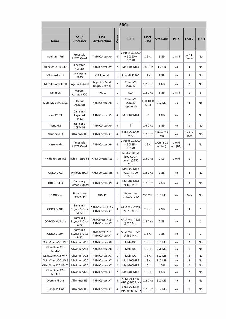
SBCs
Name
SoC/ Processor
CPU Architecture C
ore
s
GPU Clock Rate
Size RAM PCIe USB 2 USB 3
Inventami Full Freescale
i.MX6 Quad ARM Cortex-A9 4
Vivante GC2000 + GC335 +
GC320
1 GHz 1 GB 1 mini 2 + 1
header No
MarsBoard RK3066 Rockchip RK3066
ARM Cortex-A9 2 Mali-400MP4 1.6 GHz 1-2 GB No 4 No
MinnowBoard Intel Atom
E640 x86 Bonnell 1 Intel GMA600 1 GHz 1 GB No 2 No
MIPS Creator CI20 Ingenic JZ4780 Ingenic XBurst (mips32 rev.2)
2 PowerVR SGX540
1.2 GHz 1 GB No 2 No
MiraBox Marvell
Armada 370 ARMv7 1 N/A 1.2 GHz 1 GB 1 mini 1 3
MYIR MYD-AM335X TI Sitara AM335x
ARM Cortex-A8 1
PowerVR SGX530
(optional)
800-1000 MHz
512 MB No 4 No
NanoPC-T1
Samsung Exynos 4
(4412) ARM Cortex-A9 4 Mali-400MP4 ? 1 GB No 2 No
NanoPi 2 Samsung S5P4418
ARM Cortex-A9 4 ? 1.4 GHz 1 GB No 1 No
NanoPi NEO Allwinner H3 ARM Cortex-A7 4 ARM Mali-400
MP2 1.2 GHz
256 or 512 MB
No 1 + 2 on
pads No
Nitrogen6x Freescale
i.MX6 Quad ARM Cortex-A9 4
Vivante GC2000 + GC355 +
GC320
1 GHz 1 GB (2 GB
option) 1 mini
opt.[94] 2 No
Nvidia Jetson TK1 Nvidia Tegra K1 ARM Cortex-A15 5
Nvidia GK20A (192 CUDA
cores) @950 MHz
2.3 GHz 2 GB 1 mini 1 1
ODROID-C2 Amlogic S905 ARM Cortex-A53 4
Mali-450MP3 +2VS @700
MHz
1.5 GHz 2 GB No 4 No
ODROID-U3 Samsung
Exynos 4 Quad ARM Cortex-A9 4
Mali-400MP4 @440 MHz
1.7 GHz 2 GB No 3 No
ODROID-W
Broadcom BCM2835
ARM11 1
Broadcom
VideoCore IV
700 MHz 512 MB No Pads No
ODROID-XU3
Samsung Exynos 5 Octa
(5422)
ARM Cortex-A15 + ARM Cortex-A7
8 ARM Mali-T628
@695 MHz 2 GHz 2 GB No 4 1
ODROID-XU3 Lite
Samsung Exynos 5 Octa
(5422)
ARM Cortex-A15 + ARM Cortex-A7
8 ARM Mali-T628
@695 MHz 1.8 GHz 2 GB No 4 1
ODROID-XU4
Samsung Exynos 5 Octa
(5422)
ARM Cortex-A15 + ARM Cortex-A7
8 ARM Mali-T628
@695 MHz 2 GHz 2 GB No 1 2
OLinuXino A10 LIME Allwinner A10 ARM Cortex-A8 1 Mali-400 1 GHz 512 MB No 2 No
OLinuXino A13 MICRO
Allwinner A13 ARM Cortex-A8 1 Mali-400 1 GHz 256 MB No 1 No
OLinuXino A13 WIFI Allwinner A13 ARM Cortex-A8 1 Mali-400 1 GHz 512 MB No 3 No
OLinuXino A20 LIME Allwinner A20 ARM Cortex-A7 2 Mali-400MP2 1 GHz 512 MB No 2 No
OLinuXino A20 LIME2 Allwinner A20 ARM Cortex-A7 2 Mali-400MP2 1 GHz 1 GiB No 2 No
OLinuXino A20 MICRO
Allwinner A20 ARM Cortex-A7 2 Mali-400MP2 1 GHz 1 GB No 2 No
Orange Pi Lite Allwinner H3 ARM Cortex-A7 4 ARM Mali-400
MP2 @600 MHz 1.2 GHz 512 MB No 2 No
Orange Pi One Allwinner H3 ARM Cortex-A7 4 ARM Mali-400
MP2 @600 MHz 1.2 GHz 512 MB No 1 No
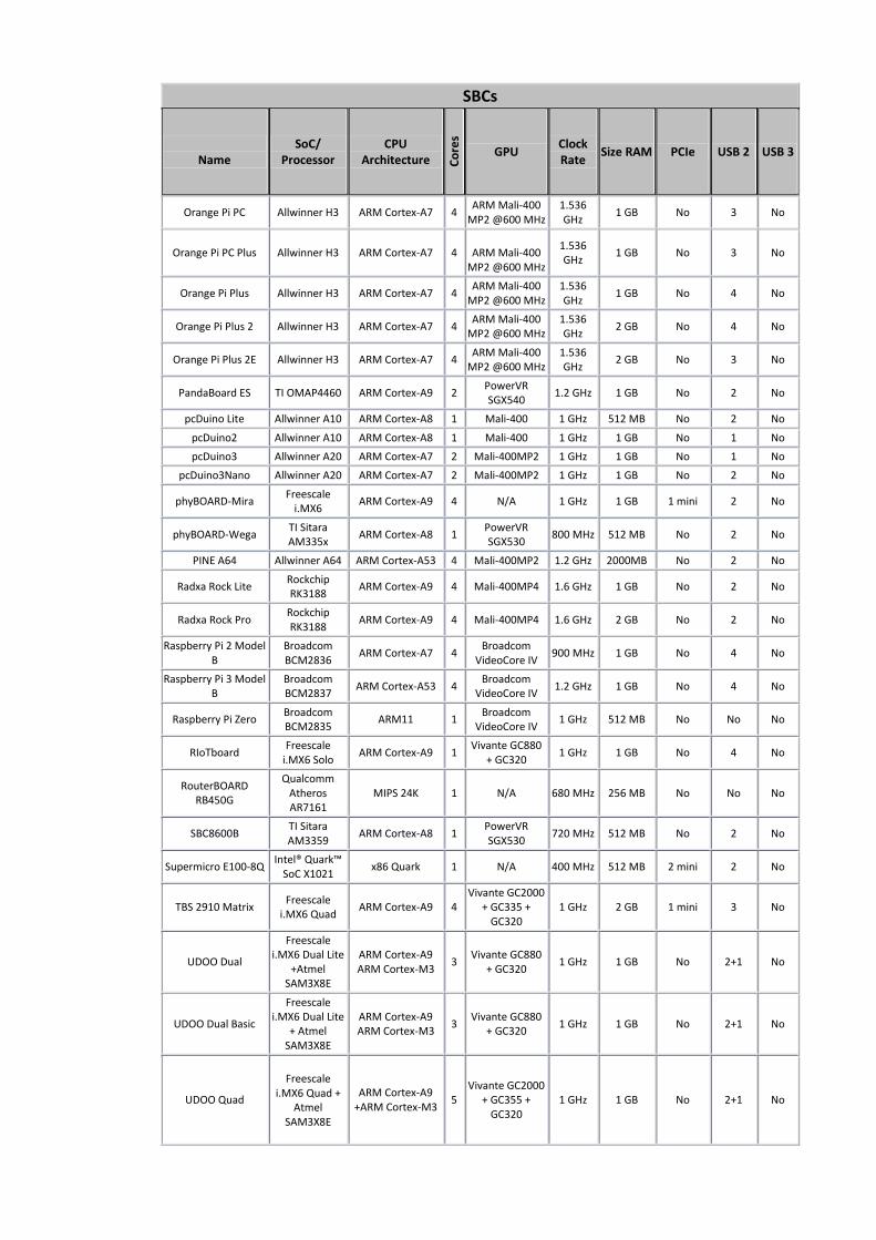
SBCs
Name
SoC/ Processor
CPU Architecture C
ore
s
GPU Clock Rate
Size RAM PCIe USB 2 USB 3
Orange Pi PC Allwinner H3 ARM Cortex-A7 4 ARM Mali-400
MP2 @600 MHz
1.536 GHz
1 GB No 3 No
Orange Pi PC Plus Allwinner H3 ARM Cortex-A7 4
ARM Mali-400
MP2 @600 MHz
1.536 GHz
1 GB No 3 No
Orange Pi Plus Allwinner H3 ARM Cortex-A7 4 ARM Mali-400
MP2 @600 MHz
1.536 GHz
1 GB No 4 No
Orange Pi Plus 2 Allwinner H3 ARM Cortex-A7 4 ARM Mali-400
MP2 @600 MHz
1.536 GHz
2 GB No 4 No
Orange Pi Plus 2E Allwinner H3 ARM Cortex-A7 4 ARM Mali-400
MP2 @600 MHz
1.536 GHz
2 GB No 3 No
PandaBoard ES TI OMAP4460 ARM Cortex-A9 2 PowerVR SGX540
1.2 GHz 1 GB No 2 No
pcDuino Lite Allwinner A10 ARM Cortex-A8 1 Mali-400 1 GHz 512 MB No 2 No
pcDuino2 Allwinner A10 ARM Cortex-A8 1 Mali-400 1 GHz 1 GB No 1 No
pcDuino3 Allwinner A20 ARM Cortex-A7 2 Mali-400MP2 1 GHz 1 GB No 1 No
pcDuino3Nano Allwinner A20 ARM Cortex-A7 2 Mali-400MP2 1 GHz 1 GB No 2 No
phyBOARD-Mira Freescale
i.MX6 ARM Cortex-A9 4 N/A 1 GHz 1 GB 1 mini 2 No
phyBOARD-Wega TI Sitara AM335x
ARM Cortex-A8 1 PowerVR SGX530
800 MHz 512 MB No 2 No
PINE A64 Allwinner A64 ARM Cortex-A53 4 Mali-400MP2 1.2 GHz 2000MB No 2 No
Radxa Rock Lite Rockchip RK3188
ARM Cortex-A9 4 Mali-400MP4 1.6 GHz 1 GB No 2 No
Radxa Rock Pro Rockchip RK3188
ARM Cortex-A9 4 Mali-400MP4 1.6 GHz 2 GB No 2 No
Raspberry Pi 2 Model B
Broadcom BCM2836
ARM Cortex-A7 4 Broadcom
VideoCore IV 900 MHz 1 GB No 4 No
Raspberry Pi 3 Model B
Broadcom BCM2837
ARM Cortex-A53 4 Broadcom
VideoCore IV 1.2 GHz 1 GB No 4 No
Raspberry Pi Zero Broadcom BCM2835
ARM11 1 Broadcom
VideoCore IV 1 GHz 512 MB No No No
RIoTboard Freescale
i.MX6 Solo ARM Cortex-A9 1
Vivante GC880 + GC320
1 GHz 1 GB No 4 No
RouterBOARD RB450G
Qualcomm Atheros AR7161
MIPS 24K 1 N/A 680 MHz 256 MB No No No
SBC8600B TI Sitara AM3359
ARM Cortex-A8 1 PowerVR SGX530
720 MHz 512 MB No 2 No
Supermicro E100-8Q Intel® Quark™
SoC X1021 x86 Quark 1 N/A 400 MHz 512 MB 2 mini 2 No
TBS 2910 Matrix Freescale
i.MX6 Quad ARM Cortex-A9 4
Vivante GC2000 + GC335 +
GC320
1 GHz 2 GB 1 mini 3 No
UDOO Dual
Freescale i.MX6 Dual Lite
+Atmel SAM3X8E
ARM Cortex-A9 ARM Cortex-M3
3 Vivante GC880
+ GC320 1 GHz 1 GB No 2+1 No
UDOO Dual Basic
Freescale i.MX6 Dual Lite
+ Atmel SAM3X8E
ARM Cortex-A9 ARM Cortex-M3
3 Vivante GC880
+ GC320 1 GHz 1 GB No 2+1 No
UDOO Quad
Freescale
i.MX6 Quad + Atmel
SAM3X8E
ARM Cortex-A9 +ARM Cortex-M3
5
Vivante GC2000 + GC355 +
GC320
1 GHz 1 GB No 2+1 No

SBCs
Name
SoC/ Processor
CPU Architecture C
ore
s
GPU Clock Rate
Size RAM PCIe USB 2 USB 3
UP Intel x5-Z8350 x86-64 4
Intel® HD 400 Graphics, 12 EU
GEN 8, up to 500 MHz
1.44 GHz 4 GB No 4+2 1
Utilite Pro Freescale
i.MX6 Quad ARM Cortex-A9 4
Vivante GC2000 + GC355 +
GC320
1.2 GHz 2 GB No 4 No
Utilite Standard Freescale
i.MX6 Dual ARM Cortex-A9 2
Vivante GC2000 + GC355 +
GC320
1 GHz 2 GB No 4 No
Utilite Value Freescale
i.MX6 Solo ARM Cortex-A9 1
Vivante GC880 + GC320
1 GHz 512 MB No 4 No
Wandboard Dual Freescale
i.MX6 Dual ARM Cortex-A9 2
Vivante GC880 + GC320
1 GHz 1 GB No 1 No
Wandboard Quad Freescale
i.MX6 Quad ARM Cortex-A9 4
Vivante GC2000 + GC355 +
GC320
1 GHz 2 GB No 1 No
Wandboard Solo Freescale
i.MX6 Solo ARM Cortex-A9 1
Vivante GC880 + GC320
1 GHz 512 MB No 1 No
SBCs
Name Onboard storage
Flash slots SA
TA
Eth
ern
et
Wif
i Blue -tooth
I 2 C
S P I
G P I O
An
alo
g
Other interfaces
Web page Price
armStoneA5 1GB Flash µSD Slot No 10/ 100
No No
Y e s
Y e s
? ?
CAN, UART, Audio, Digital I/O, Touch
Panel
https://www.fs-net.de/en/products/armstone/armstonea
5/
179,00 €
armStoneA8 1GB Flash No No 10/ 100
No No
Y e s
Y e s
? ?
CAN, Audio, Digital I/O, Touch
Panel
https://www.fs-net.de/en/products/armstone/armstonea
8/
?
armStoneA9 1GB Flash SD Yes GbE No No
Y e s
Y e s
? ?
CAN, UART, Audio, Digital I/O, Touch
Panel
https://www.fs-net.de/en/products/armstone/armstonea
9/
299,00 €
Arndale Board 4GB eMMC microSD SATA 3.0
100
a/b/g/n
(AR6003)
4.0 BR/EDR + BLE
? ?
O P t.
? JTAG, RS232, MIPI
DSI, Audio
http://www.arndaleboard.org/wiki/index
.php/Main_Page
?
Banana Pi No SD SATA 2.0
GbE No No
Y e s
Y e s
80
12-Bit-ADC
CSI, UART
http://www.bananapi.org/p/product.ht
ml 35 €
Banana Pi M2 No microSD No GbE a/b/g
/n No
Y e s
Y e s
40
12-Bit-ADC
CSI, UART http://www.banana-
pi.org/m2.html 60 €
Banana Pi M3 No microSD SATA 2.0
GbE a/b/g
/n 4.0
Y e s
Y e s
40
12-Bit-ADC
CSI, UART http://www.banana-
pi.org/m3.html 109,99 €
BeagleBoard 512MB Flash SD No No No No ? ?
Y e s
No
https://beagleboard.org/beagleboard
118,38 €
BeagleBoard-xM ? SD No 10/ 100
No No ? ? ? ? ? https://beagleboard.org/beagleboard-xm
141,11 €
BeagleBone 4GB Flash microSD No 10/ 100
No No
Y e s
Y e s
66
12-Bit-ADC
CAN, UART https://beagleboard.
org/bone-original 84 €

SBCs
Name Onboard storage
Flash slots SA
TA
Eth
ern
et
Wif
i Blue -tooth
I 2 C
S P I
G P I O
An
alo
g
Other interfaces
Web page Price
BeagleBone Black 4GB eMMC microSD No 10/ 100
No No
Y e s
Y e s
66 12-bit ADC
CAN, UART https://beagleboard.
org/black 43 €
Boardcon EM210 4GB eMMC microSD No 10/100 b/g No
Y e s
Y e s
Y e s
ADCDAC
PWM
UART, Audio, Digital I/O, Touch
Panel, JTAG
http://www.boardcon.com/EM210/
?
Boardcon EM3288 8GB eMMC microSD Yes GbE b/g/n 4.0
Y e s
Y e s
Y e s
ADC
UART, MIPI, I2S, Audio, Digital I/O,
Touch Panel
http://www.boardcon.com/EM3288_SBC
/
?
C.H.I.P. 4 GB No No No a/b/g
/n 4.0
Y e s
?
Y e s
?
UART, PWM https://getchip.com/
pages/chip 8,5€
CuBox-i2 No microSD No 10/100 n opt. Opt. No No ? No S/PDIF, CIR rx
https://www.solid-run.com/freescale-imx6-family/cubox-
i/cubox-i-specifications/
103,50 €
CuBox-i2eX No microSD eSATA
2.0 GbE n opt. Opt. No No ? No S/PDIF, CIR rx/tx
https://www.solid-run.com/freescale-imx6-family/cubox-
i/cubox-i-specifications/
122,33 €
CuBox-i4Pro No microSD
E SATA 2.0
GbE
b/g/n (BCM4329)
2.1 + EDR No No ? No S/PDIF, CIR rx/tx
https://www.solid-run.com/freescale-imx6-family/cubox-
i/cubox-i-specifications/
131,74 €
Dragonboard 410c 8GB eMMC microSD No No
a/b/g/n ( 2.4
GHz )
4.1
Y e s
Y e s
12 No
UART, I2S, 2-lane + 4-lane CSI, USB (expansion), GPS
(onboard antenna)
https://developer.qualcomm.com/hardw
are/dragonboard-410c
71 €
DreamPlug 4GB microSD microSD eSATA
2.0 2x GbE
b/g/n (88W8787)
3.0 + HS No No 7 No JTAG, UART
https://www.globalscaletechnologies.com/p-54-dreamplug-
devkit.aspx
149,63 €
Graperain G4418 SBC 8GB eMMC 2x TF No GbE
b/g/n (RTL8723BU) ( 2.4
GHz)
4.0 + LE (RTL8723B
U)
Y e s
Y e s
Y e s
P WM
UART
https://www.graperain.com/ARM-
Embedded-S5P4418-Single-Board-
Computer/
?
Graperain G6818 SBC 8GB eMMC 2x TF No GbE
b/g/n (RTL8723BU) ( 2.4
GHz)
4.0 + LE (RTL8723B
U)
Y e s
Y e s
Y e s
P WM
UART
https://www.graperain.com/ARM-
Embedded-S5P6818-Single-Board-
Computer/
?
HiKey 4GB eMMC microSD No No a/b/g
/n 4.0
Y e s
Y e s
12 No UART, USB (expansion)
http://www.96boards.org/product/hikey/
71 €
HummingBoard-i2eX No microSD
(UHS) mSAT
A GbE No No
Y e s
Y e s
8 No CIR rx, CSI-2,
FlexCAN, UART
https://www.solid-run.com/product/hummingboard-carrier-pro/#configuration
79 €
Intel Galileo Gen 2 8MB Flash + 8 KB EEPROM
SD No 10/100 No No
Y e s
Y e s
20
12-bit ADC,
6 PWM
Arduino 1.0 headers, JTAG, 6x
UART
http://www.intel.com/content/www/us/en/embedded/produ
cts/galileo/galileo-overview.html
64 €
Inventami Entry 4GB eMMC microSD m
SATA GbE No No
Y e s
Y e s
46 No
FPGA ETH, FPGA GPIO, CAN, UART,
RS-232, LVDS+Touch Panel
http://www.inventami.com/
?
Inventami Full 16GB eMMC microSD m
SATA GbE No No
Y e s
Y e s
50 No
FPGA ETH, FPGA
GPIO, FPGA SerDes, CAN,
UART, RS-232, LVDS+Touch Pane
l
http://www.inventami.com/
?

SBCs
Name Onboard storage
Flash slots SA
TA
Eth
ern
et
Wif
i Blue -tooth
I 2 C
S P I
G P I O
An
alo
g
Other interfaces
Web page Price
MarsBoard RK3066 4GB Flash microSD No 10/ 100
b/g/n (RTL8188)
No No No ? No CIF, UART
http://www.marsboard.com/marsboard_rk3066_feature.html
55 €
MinnowBoard No microSD Yes GbE No No No No 14 No JTAG
http://wiki.minnowboard.org/MinnowBo
ard_Wiki_Home
?
MIPS Creator CI20 8GB Flash SD No 10/ 100
b/g/n (BCM4330)
4.0 (BCM4330)
Y e s
Y e s
25
A D C
UART, JTAG http://creatordev.io/
ci20 72 €
MiraBox 1GB Flash microSD No 2x GbE
b/g/n (88W8787)
3.0 No No 40 No JTAG
https://www.globalscaletechnologies.co
m/p-58-mirabox-development-
kit.aspx
140,22 €
MYIR MYD-AM335X 512MB Flash SD No
2x GbE
No No
Y e s
Y e s
No ADCPWM
CAN, 2x RS-232, RS-485
http://www.myirtech.com/list.asp?id=46
6 131,64 €
NanoPC-T1 8GB eMMC SD No 10/100 No No No No ? No CIF, UART
http://www.nanopc.org/NanoPC-
T1_Feature.html ?
NanoPi 2 No 2x microSD No No
b/g/n (AP62
12)
4.0 + LE (AP6212)
Y e s
Y e s
Y e s
P WM
UART http://nanopi.io/nan
opi2.html 30 €
NanoPi NEO No microSD No 10/100 No No
Y e s
Y e s
Y e s
P WM
UART http://nanopi.io/nan
opi-neo.html ?
Nitrogen6x No 2x microSD SATA GbE
b/g/n (WL1271)
Opt. Y e s
No ? No CAN-2, JTAG, extra
USB header
https://boundarydevices.com/product/nitrogen6x-board-imx6-arm-cortex-a9-sbc/
211,74 €
Nvidia Jetson TK1 16GB eMMC SD Yes GbE No No
Y e s
Y e s
7 No CSI-2, HSIC, JTAG,
RS-232, UART
http://www.nvidia.com/object/jetson-
tk1-embedded-dev-kit.html
181,83 €
ODROID-C2 eMMC module
opt. microSD No
10 / 100 / 1000
No No
Y e s
Y e s
32
2x 12-bit
ADC PWM
UART, IR, Real-time clock battery
connector
http://www.hardkernel.com/main/products/prdt_info.php?g_code=G14545721643
8
40 €
ODROID-U3 eMMC module
opt. microSD No
10/ 100
No No
Y e s
No
Y e s
No
UART, Real-time clock battery
connector
http://www.hardkernel.com/main/products/prdt_info.php?g_code=g13874569627
5
65 €
ODROID-W eMMC module
opt. microSD No No No No
Y e s
Y e s
32
2x 12-bit
ADC PWM
Real-time clock battery connector,
LiPo battery connector
http://www.hardkernel.com/main/products/prdt_info.php?g_code=g14061018949
0
28 €
ODROID-XU3 eMMC module
opt. microSD No
10/ 100
(LAN9514)
No No
Y e s
Y e s
Y e s
A D C
UART, Real-time clock battery
connector
http://www.hardkernel.com/main/products/prdt_info.php?g_code=g14044826712
7
169,51 €
ODROID-XU3 Lite eMMC module
opt. microSD No
10/ 100
(LAN9514)
No No
Y e s
Y e s
Y e s
A D C
UART, Real-time clock battery
connector
http://www.hardkernel.com/main/products/prdt_info.php?g_code=G14135188095
5
94 €
ODROID-XU4 eMMC module
opt. microSD No
10 / 100 / 1000
(LAN9514)
No No
Y e s
Y e s
Y e s
A D C
UART, Real-time clock battery
connector
http://www.hardkernel.com/main/products/prdt_info.php?g_code=G14
3452239825
70 €
OLinuXino A10 LIME No microSD Yes 100 No No
Y e s
Y e s
134 P
WM 6x UART
https://www.olimex.com/Products/OLinu
Xino/A10/A10-OLinuXino-
LIME/open-source-hardware
30 €

SBCs
Name Onboard storage
Flash slots SA
TA
Eth
ern
et
Wif
i Blue -tooth
I 2 C
S P I
G P I O
An
alo
g
Other interfaces
Web page Price
OLinuXino A13 MICRO
No microSD No No No No ? ? 142 No ?
https://www.olimex.com/Products/OLinu
Xino/A13/A13-OLinuXino-
MICRO/open-source-hardware
35 €
OLinuXino A13 WIFI 4GB Flash microSD No No
b/g/n (RTL8188)
No ? ? 142 No ?
https://www.olimex.com/Products/OLinu
Xino/A13/A13-OLinuXino-
WIFI/open-source-hardware
55 €
OLinuXino A20 LIME 4GB Flash opt. microSD Yes 100 No No ? ? 160 No UART, UEXT
https://www.olimex.com/Products/OLinu
Xino/A20/A20-OLinuXino-
LIME/open-source-hardware
33 €
OLinuXino A20 LIME2 4GB Flash opt. microSD Yes 1000 No No ? ? 160 No UART, UEXT
https://www.olimex.com/Products/OLinu
Xino/A20/A20-OLinuXIno-
LIME2/open-source-hardware
45 €
OLinuXino A20 MICRO
4GB Flash opt. microSD,
SD Yes 100 No No ? ? 160 No UART, UEXT
https://www.olimex.com/Products/OLinu
Xino/A20/A20-OLinuXino-
MICRO/open-source-hardware
55 €
Orange Pi Lite No microSD No No
b/g/n (RTL8189FT
V)
No
Y e s
Y e s
Y e s
? CSI, IR, UART http://www.orangep
i.org/orangepilite/ 11 €
Orange Pi One No microSD No 10/ 100
No No
Y e s
Y e s
Y e s
? CSI, UART http://www.orangepi.org/orangepione/
9,5 €
Orange Pi PC No microSD No 10/ 100
No No
Y e s
Y e s
Y e s
? CSI, IR, UART http://www.orangep
i.org/orangepipc/ 14 €
Orange Pi PC Plus 8GB Flash microSD No 10/ 100
b/g/n (RTL8189FT
V)
No
Y e s
Y e s
Y e s
? CSI, IR, UART
http://www.orangepi.org/orangepipcplus
/
19 €
Orange Pi Plus 8GB Flash microSD SATA 2.0
GbE
b/g/n (RTL8189ET
V)
No
Y e s
Y e s
Y e s
? CSI, IR, UART http://www.orangep
i.org/ 19 €
Orange Pi Plus 2 16GB eMMC microSD SATA 2.0
GbE
b/g/n (RTL8189ET
V)
No
Y e s
Y e s
Y e s
? CSI, IR, UART http://www.orangepi.org/orangepiplus2/
46 €
Orange Pi Plus 2E 16GB eMMC microSD No GbE
b/g/n (RTL8189FT
V)
No
Y e s
Y e s
Y e s
? CSI, IR, UART
http://www.orangepi.org/orangepiplus2e
/
33 €
PandaBoard ES No SDHC No 10/ 100
b/g/n (WL1271)
2.1 + EDR
Y e s
No
Y e s
No JTAG, RS-232,
UART
http://pandaboard.org/content/pandabo
ard-es
190,92 €
pcDuino Lite No microSD No 10/ 100
No No
Y e s
Y e s
22 ADC
PWM
Arduino 1.0 headers
http://www.linksprite.com/linksprite-
pcduino-lite/
28 €
pcDuino2 4GB Flash microSD No 10/ 100
b/g/n (RTL8188)
No
Y e s
Y e s
22 ADC
PWM
Arduino 1.0 headers
http://www.linksprite.com/linksprite-
pcduino2/
46 €
pcDuino3 4GB Flash microSD Yes 10/ 100
b/g/n (RTL8188)
No
Y e s
Y e s
22 ADC
PWM
Arduino 1.0 headers
http://www.linksprit
e.com/linksprite-pcduino3/
47 €

SBCs
Name Onboard storage
Flash slots SA
TA
Eth
ern
et
Wif
i Blue -tooth
I 2 C
S P I
G P I O
An
alo
g
Other interfaces
Web page Price
pcDuino3Nano 4GB Flash microSD Yes GbE No No
Y e s
Y e s
22 ADC
PWM
Arduino 1.0 headers
http://www.linksprite.com/linksprite-pcduino3-nano/
38 €
phyBOARD-Mira 1GB Flash, 4 kB
EEPROM microSD Yes GbE Yes No
Y e s
Y e s
Y e s
PWM
CAN, RS232, Digital I/O, Audio,
Camera, UART, JTAG
http://www.phytec.de/produkt/single-
board-computer/phyboard-
mira/
166,00 €
phyBOARD-Wega 512MB Flash,4
kB EEPROM microSD No 10/ 100 No No
Y e s
Y e s
Y e s
ADC PWM
CAN, RS232, Audio, UART, JTAG, MMC
http://www.phytec.eu/product/single-
board-computer/phyboard-
wega/
130,00 €
PINE A64 No microSD No 10/ 100 Opt. Opt. Y e s
Y e s
46 No
https://www.pine64.org/
28 €
Radxa Rock Lite 4GB Flash microSD (SDXC)
No 10/ 100
b/g/n (RTL8188)
No
Y e s
Y e s
80 ADC
PWM UART
http://wiki.radxa.com/Rock/specification
76 €
Radxa Rock Pro 8GB Flash microSD (SDXC)
No 10/ 100
b/g/n (RTL8723)
4.0 (Works on android but not on
linux)
Y e s
Y e s
80 ADC
PWM UART
http://wiki.radxa.com/Rock/specification
?
Raspberry Pi 2 Model B
No microSD No 10/ 100
No No
Y e s
Y e s
17 No UART, CSI, DSI
https://www.raspberrypi.org/products/raspberry-pi-2-model-
b/
34 €
Raspberry Pi 3 Model B
No microSD No 10/ 100
b/g/n 4.1
Y e s
Y e s
17 No UART, CSI, DSI
https://www.raspberrypi.org/products/raspberry-pi-3-model-
b/
35 €
Raspberry Pi Zero No microSD No No No No
Y e s
Y e s
17 No UART, DSI (only newer versions)
https://www.raspberrypi.org/products/pi-
zero/ 4,7 €
RIoTboard 4GB Flash microSD and SD
No GbE No No
Y e s
Y e s
10 P
WM CSI, UART http://riotboard.org/ 73 €
RouterBOARD RB450G
512MB Flash microSD No
5x GbE (AR8316
) No No No No No No JTAG, RS-232
https://routerboard.com/RB450G
94 €
SBC8600B 512MB Flash microSD No 2x GbE No No No
Y e s
Y e s
12-bit ADC
CAN-2, RS-232, RS-485
http://www.ti.com/devnet/docs/catalog/endequipmentproductfolder.tsp?actionPerformed=productFolder&productId=211
20
136,46 €
Supermicro E100-8Q No microSDHC No 2 x 10/
100 No No No No No No
RS232 (DB9), RS285 (screw
terminal), ZigBee module socket
http://www.supermicro.com/products/system/Compact/IoT/S
YS-E100-8Q.cfm
?
TBS 2910 Matrix 16GB eMMC microSD and SD
SATA 2.0
GbE b/g/n No
Y e s
No No Yes UART
http://www.tbsdtv.com/products/tbs2910-matrix-arm-mini-
pc.html
142,04 €
UDOO Dual No microSD No GbE
n (RT53
70) No
Y e s
Y e s
76
10-bit ADC
PWM
Arduino 1.0 headers
http://www.udoo.org/udoo-dual-and-
quad/
105,91 €
UDOO Dual Basic No microSD No No No No
Y e s
Y e s
76
10-bit ADC
PWM
Arduino 1.0 headers
http://shop.udoo.org/eu/quad-
dual/udoo-dual-basic.html
94 €
UDOO Quad No microSD SATA GbE
n (RT53
70) No
Y e s
Y e s
76
10-bit ADC
PWM
Arduino 1.0 headers
http://www.udoo.org/udoo-dual-and-
quad/ 127,85 €
UP 16/32/64 GB
eMMC No No GbE No No
Y e s
Y e s
Y e s
No 40-pin GP-bus
http://www.up-board.org/up/
122,17 €

SBCs
Name Onboard storage
Flash slots SA
TA
Eth
ern
et
Wif
i Blue -tooth
I 2 C
S P I
G P I O
An
alo
g
Other interfaces
Web page Price
Utilite Pro 32GB mSATA microSD (SDXC)
m SATA
2x GbE
b/g/n (88W8787)
3.0 No No No No 2x RS-232
http://www.compulab.co.il/utilite-
computer/web/utilite-models
242,44 €
Utilite Standard 8GB microSD microSD (SDXC)
m SATA
2x GbE
b/g/n (88W8787)
3.0 No No No No 2x RS-232
http://www.compulab.co.il/utilite-
computer/web/utilite-models
188,46 €
Utilite Value 4GB microSD microSD (SDXC)
m SATA
GbE No No No No No No 2x RS-232
http://www.compulab.co.il/utilite-
computer/web/utilite-models
126,90 €
Wandboard Dual No 2x microSD No GbE
n (BCM4329)
Yes
Y e s
Y e s
10 No UART http://www.wandbo
ard.org/ 94 €
Wandboard Quad No 2x microSD Yes GbE
n (BCM4329)
Yes
Y e s
Y e s
10 No UART http://www.wandbo
ard.org/ 122,17 €
Wandboard Solo No 2x microSD No GbE No No
Y e s
Y e s
10 No UART http://www.wandbo
ard.org/ 75 €
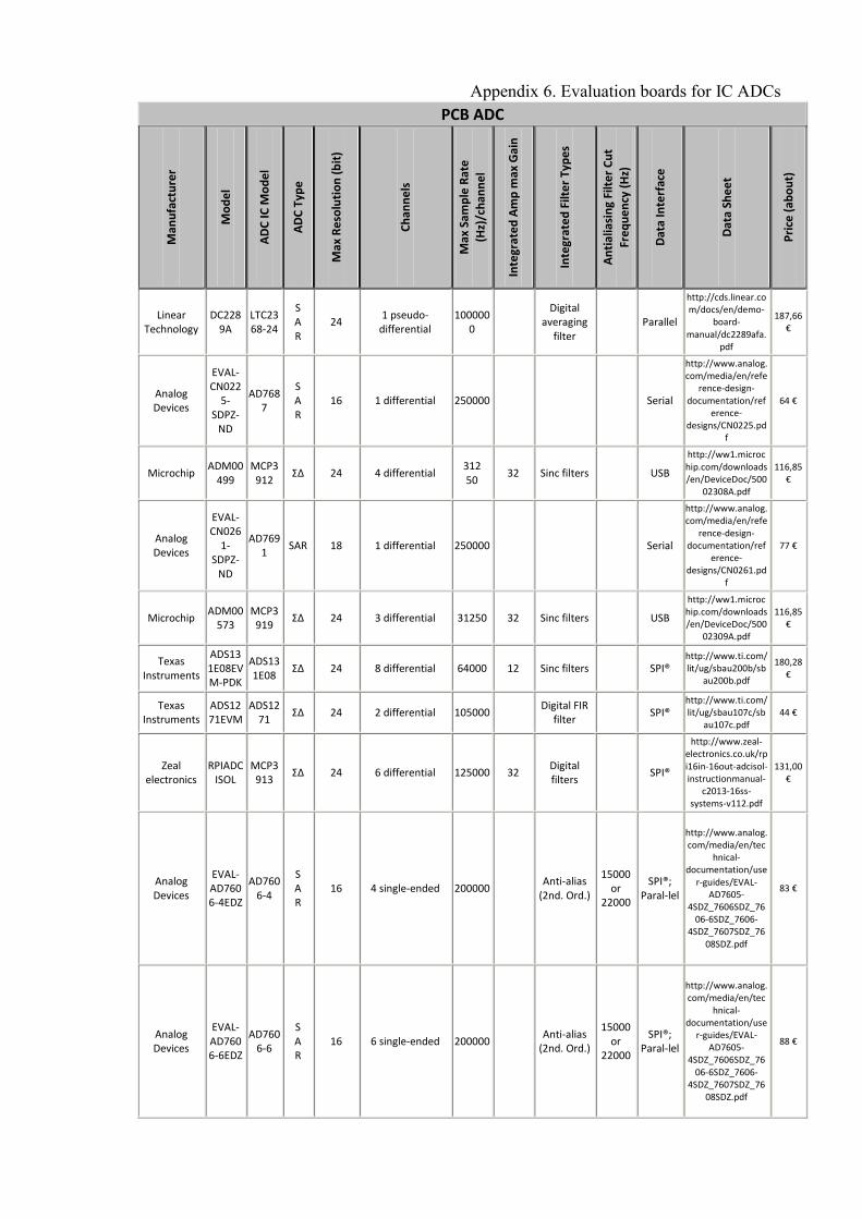
Appendix 6. Evaluation boards for IC ADCs
PCB ADC
Man
ufa
ctu
rer
Mo
de
l
AD
C IC
Mo
de
l
AD
C T
ype
Max
Re
solu
tio
n (
bit
)
Ch
ann
els
Max
Sam
ple
Rat
e
(Hz)
/ch
ann
el
Inte
grat
ed
Am
p m
ax G
ain
Inte
grat
ed
Filt
er
Typ
es
An
tia
liasi
ng
Filt
er
Cu
t
Fre
qu
en
cy (
Hz)
Dat
a In
terf
ace
Dat
a Sh
ee
t
Pri
ce (
abo
ut)
Linear Technology
DC2289A
LTC2368-24
S A R
24 1 pseudo-
differential 100000
0
Digital averaging
filter
Parallel
http://cds.linear.com/docs/en/demo-
board-manual/dc2289afa.
187,66 €
Analog Devices
EVAL-CN022
5-SDPZ-
ND
AD7687
S A R
16 1 differential 250000
Serial
http://www.analog.com/media/en/refe
rence-design-documentation/ref
erence-designs/CN0225.pd
f
64 €
Microchip ADM00
499
MCP3912
ΣΔ 24 4 differential 312 50
32 Sinc filters
USB
http://ww1.microchip.com/downloads/en/DeviceDoc/500
02308A.pdf
116,85 €
Analog Devices
EVAL-CN026
1-SDPZ-
ND
AD7691
SAR 18 1 differential 250000
Serial
http://www.analog.com/media/en/refe
rence-design-documentation/ref
erence-designs/CN0261.pd
f
77 €
Microchip ADM00
573
MCP3919
ΣΔ 24 3 differential 31250 32 Sinc filters
USB
http://ww1.microchip.com/downloads/en/DeviceDoc/500
02309A.pdf
116,85 €
Texas Instruments
ADS131E08EVM-PDK
ADS131E08
ΣΔ 24 8 differential 64000 12 Sinc filters
SPI® http://www.ti.com/lit/ug/sbau200b/sb
au200b.pdf
180,28 €
Texas Instruments
ADS1271EVM
ADS1271
ΣΔ 24 2 differential 105000
Digital FIR filter
SPI® http://www.ti.com/lit/ug/sbau107c/sb
au107c.pdf 44 €
Zeal electronics
RPIADCISOL
MCP3913
ΣΔ 24 6 differential 125000 32 Digital filters
SPI®
http://www.zeal-electronics.co.uk/rpi16in-16out-adcisol-instructionmanual-
c2013-16ss-systems-v112.pdf
131,00 €
Analog Devices
EVAL-AD7606-4EDZ
AD7606-4
S A R
16 4 single-ended 200000
Anti-alias (2nd. Ord.)
15000 or
22000
SPI®; Paral-lel
http://www.analog.com/media/en/tec
hnical-documentation/use
r-guides/EVAL-AD7605-
4SDZ_7606SDZ_7606-6SDZ_7606-
4SDZ_7607SDZ_7608SDZ.pdf
83 €
Analog Devices
EVAL-AD7606-6EDZ
AD7606-6
S A R
16 6 single-ended 200000
Anti-alias (2nd. Ord.)
15000 or
22000
SPI®; Paral-lel
http://www.analog.com/media/en/tec
hnical-documentation/use
r-guides/EVAL-AD7605-
4SDZ_7606SDZ_7606-6SDZ_7606-
4SDZ_7607SDZ_7608SDZ.pdf
88 €

PCB ADC
Man
ufa
ctu
rer
Mo
de
l
AD
C IC
Mo
de
l
AD
C T
ype
Max
Re
solu
tio
n (
bit
)
Ch
ann
els
Max
Sam
ple
Rat
e
(Hz)
/ch
ann
el
Inte
grat
ed
Am
p m
ax G
ain
Inte
grat
ed
Filt
er
Typ
es
An
tia
liasi
ng
Filt
er
Cu
t
Fre
qu
en
cy (
Hz)
Dat
a In
terf
ace
Dat
a Sh
ee
t
Pri
ce (
abo
ut)
Analog Devices
EVAL-AD7606SDZ
AD7606
S A R
16 8 single-ended 200000
Anti-alias (2nd. Ord.)
15000 or
22000
SPI®; Paral-lel
http://www.analog.com/media/en/tec
hnical-documentation/use
r-guides/EVAL-AD7605-
4SDZ_7606SDZ_7606-6SDZ_7606-
4SDZ_7607SDZ_7608SDZ.pdf
55 €
Analog Devices
EVAL-CN030
3
AD7476
S A R
12 1 single-ended 100000
0 SPI®
http://www.analog.com/media/en/refe
rence-design-documentation/ref
erence-designs/CN0303.pd
f
70 €
Analog Devices
EVAL-AD760
9
AD7609
S A R
18 8 differential 200000
Amalog low pass
23000 or
32000
SPI®; QSPI™; MICRO-WIRE™;
DSP compa-
tible; Paral-lel
http://www.analog.com/en/design-
center/evaluation-hardware-and-
software/evaluation-boards-kits/EVAL-AD7609.html#eb-
overview
130,00 €
Analog Devices
EVAL-AD717
6-2
AD7176-2
ΣΔ 24 2 differential 50000
Digital filters
SPI®; QSPI™; MICRO-WIRE™;
DSP compa-
tible
http://www.analog.com/en/design-
center/evaluation-hardware-and-
software/evaluation-boards-kits/eval-ad7176-2.html#eb-
overview
76 €
Analog Devices
EVAL-AD760
8
AD7608
SAR 18 8 single-ended 200000
Analog low pass
15000 or
23000
SPI®; QSPI™; MICRO-WIRE™;
DSP compa-
tible; Paral-lel
http://www.analog.com/en/design-
center/evaluation-hardware-and-
software/evaluation-boards-kits/EVAL-AD7608.html#eb-
overview
67 €
Waveshare
Raspberry Pi High-
Precision
AD/DA Expansi
on Board
ADS1256
ΣΔ 24 8 single-ended or
4 differential 4000 64
Digital filter (5th order
sinc)
SPI®
http://www.waveshare.com/High-
Precision-AD-DA-Board.htm
28 €
Analog Devices
EVAL-CN0254-SDPZ
AD7689
SAR 16 8 single-ended or
differential 250000
Selectable one-pole low-pass
filter
SPI®
http://www.analog.com/media/en/refe
rence-design-documentation/ref
erence-designs/CN0254.pdf
74 €
Analog Devices
EVAL-CN0269-SDPZ
AD7984
SAR 18 16 single-ended or
8 differential 250000
Serial
http://www.analog.com/media/en/refe
rence-design-documentation/ref
erence-designs/CN0269.pd
f
98 €

Appendix 7. USB DAQs and oscilloscopes
USB DAQs/oscilloscopes
Man
ufa
ctu
r
er
Mo
de
l
Typ
e
Max
Re
solu
tio
n
(bit
)
Ch
ann
els
Max Sample
Rate (Hz)/ch
Integrated Amp max
Gain
Dat
a
Inte
rfac
es
Price (about)
Data Sheet
LabJack U6
D A Q
18
14 single-
ended or diffe-rential
50000 1000 SPI®; USB;
I2C 281,24 €
https://labjack.com/sites/default/files/LabJack-U6-
Datasheet-Export-20161024.pdf
LabJack T7
D A Q
16
14 single-
ended or diffe-rential
100000 1000
SPI®; USB; I2C; Wi-Fi; Ethernet
375,31 €
https://labjack.com/sites/default/files/LabJack-T7-
Datasheet-Export-20161024.pdf
Open DAQ [M] D A Q
16
8 single-ended or
diffe-rential
20000 100 USB 200,00 €
https://www.open-daq.com/productos/opend
aq-m
USB-DUX D
D A Q
12 8 single-ended
8000
USB 59,15 € http://www.linux-usb-
daq.co.uk/tech2_usbdux/
USB-DUX Fast D A Q
12
16 single-ended
3000000
USB 59,15 € http://www.linux-usb-
daq.co.uk/tech2_duxfast/
USB-DUX Sigma
D A Q
24
16 single-ended
4000
USB 118,30€
http://www.linux-usb-daq.co.uk/tech2_duxsigma
/
Data Transla-tion
DT9816
D A Q
16 6 single-ended
50000 2 USB 454,58€
http://www.datatranslation.com/Products/Low-Cost-
DAQ/DT9816
Bitscope BS05 Sco-pe
12 2 single-ended
20000000
USB 136,31 € http://www.bitscope.com/
product/BS05/?p=specs
Bitscope BS10 Sco-pe
12 2 single-ended
20000000
USB 231,18 €
http://www.bitscope.com/
product/BS10/?p=specs
NI NI
USB-6210
D A Q
16
16 single-
ended or 8 diffe-rential
250000
USB 720,00 € http://www.ni.com/pdf/m
anuals/375194c.pdf
MC
USB-1608FS-Plus
D A Q
16 8 single-ended
100000
USB 375,23 €
http://www.mccdaq.com/PDFs/specs/USB-1608FS-
Series-data.pdf

Appendix 8. Certificate of calibration (wax mounting): B&K 4394.


Appendix 9. Certificate of calibration (wax mounting): Te Connectivity ACH 01

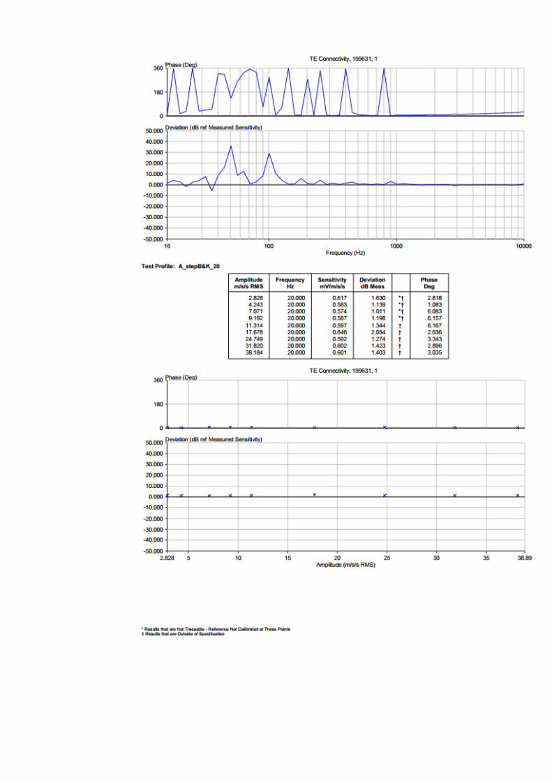
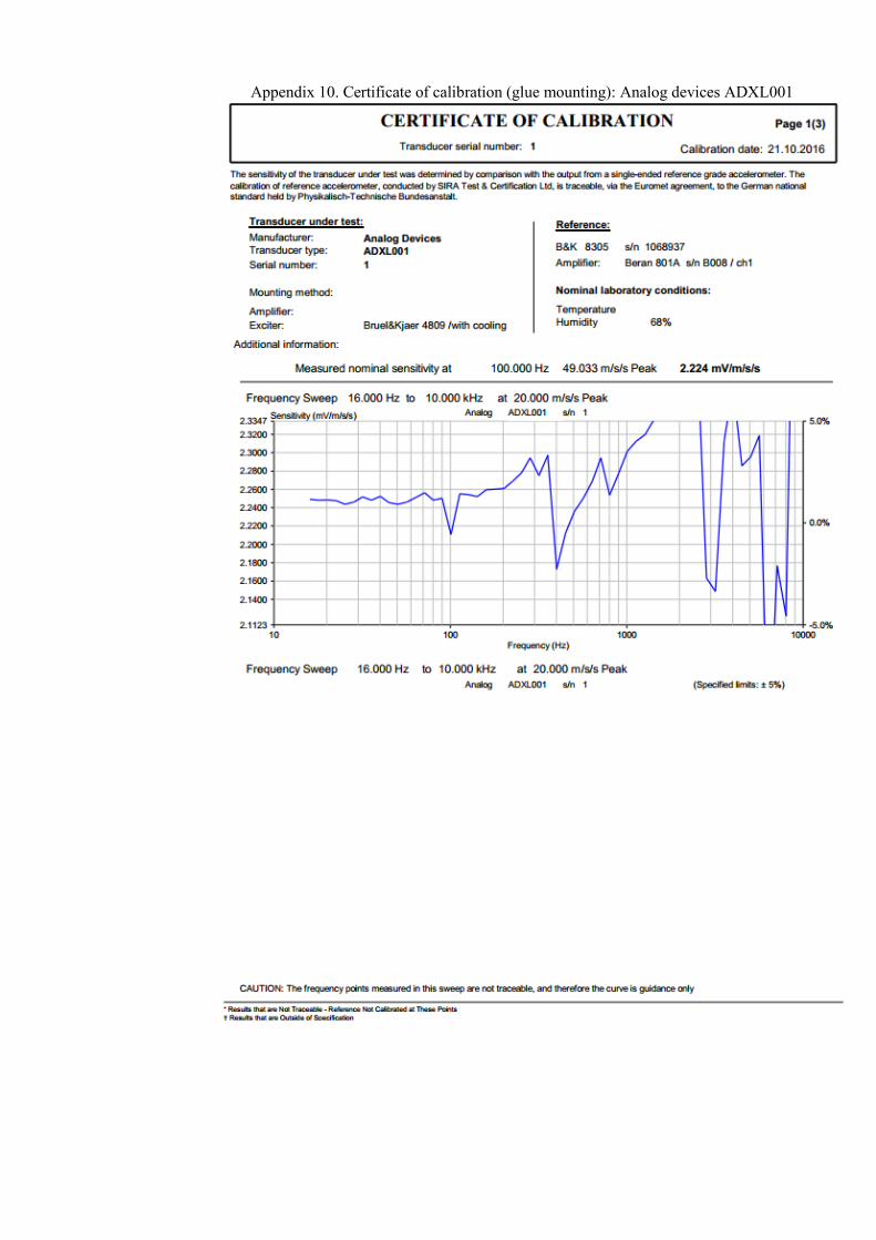
Appendix 10. Certificate of calibration (glue mounting): Analog devices ADXL001


Appendix 11. Certificate of calibration (screw mounting): Analog devices ADXL001


–––