the study of cirrus clouds using airborne and …

THE STUDY OF CIRRUS CLOUDS USING AIRBORNE AND

SATELLITE DATA

A Thesis

by

KERRY GLYNNE MEYER

Submitted to the Office of Graduate Studies ofTexas A&M University

in partial fulfillment of the requirements for the degree of

MASTER OF SCIENCE

May 2004

Major Subject: Atmospheric Sciences

THE STUDY OF CIRRUS CLOUDS USING AIRBORNE AND

SATELLITE DATA

A Thesis

by

KERRY GLYNNE MEYER

Submitted to Texas A&M Universityin partial fulfillment of the requirements

for the degree of

MASTER OF SCIENCE

Approved as to style and content by:

Ping Yang(Chair of Committee)

George Kattawar(Member)

Thomas Wilheit(Member)

Richard Orville(Head of Department)

May 2004

Major Subject: Atmospheric Sciences

iii

ABSTRACT

The Study of Cirrus Clouds Using Airborne and Satellite Data. (May 2004)

Kerry Glynne Meyer, B.S., Texas A&M University

Chair of Advisory Committee: Dr. Ping Yang

Cirrus clouds are known to play a key role in the earth’s radiation budget, yet are one

of the most uncertain components of the earth-atmosphere system. With the

development of instruments such as the Airborne Visible/Infrared Imaging Spectrometer

(AVIRIS) and the Moderate-resolution Infrared Spectroradiometer (MODIS), scientists

now have an unprecedented ability to study cirrus clouds. To aid in the understanding of

such clouds, a significant study of cirrus radiative properties has been undertaken. This

research is composed of three parts: 1) the retrieval of tropical cirrus optical thickness

using MODIS level-1b calibrated radiance data, 2) a survey of tropical cirrus cloud

cover, including seasonal variations, using MODIS level-3 global daily gridded data, and

3) the simultaneous retrieval of cirrus optical thickness and ice crystal effective diameter

using AVIRIS reflectance measurements.

iv

DEDICATION

This manuscript is dedicated to all of my family and friends who have helped and

supported me throughout the years.

v

ACKNOWLEDGEMENTS

I would like to thank my advisor, Dr. Ping Yang, for his guidance, support, ideas,

and patience throughout my work on this project. Without his aid, this thesis would

never have been finished. I greatly appreciate everything he has done for me, and for the

opportunity he has given me to continue my education. Also, I would like to thank the

members of my advisory committee, Dr. Thomas Wilheit and Dr. George Kattawar, for

showing an interest in my research, and for taking time out of their schedules to assist in

editing this manuscript.

I would like to thank Dr. Bo-Cai Gao at the Naval Research Laboratory for his help

on my projects and publications. I would like to thank Dr. Bryan Baum and Shaima

Nasiri for their help with the DISORT code. I would also like to thank Drs. Michael

King and Steve Platnick for the MODIS visualization software developed by their group.

This study was supported by NASA/EOS grant NAG5-11935, and also partially

supported by the NASA Radiation Sciences Program managed by Drs. Donald Anderson

and Hal Maring (NAG-1-02002), the National Science Foundation Physical

Meteorology Program managed by Dr. William A. Cooper (ATM-0239605), and a

subcontract (4400053274) from Science Applications International Corporation.

Last but not least, I would like to thank my family and friends, especially my mom,

my dad, my brother, and my grandparents, for all of the support they have given me

throughout the years. I would also like to thank Alison Gardner, the love of my life, for

the loving support and patience she has given me.

vi

TABLE OF CONTENTS

Page

ABSTRACT……………………………………………………………….……….. iii

DEDICATION…………………………………………………………….……….. iv

ACKNOWLEDGEMENTS……………………………………………….……….. v

TABLE OF CONTENTS…………………………………………….…………….. vi

LIST OF FIGURES……………………………………………………….……….. viii

1. INTRODUCTION……………………………………………………………… 1

2. METHODOLOGY……………………………………………………………... 5

2.1 Research Objectives……………………………………………….. 52.2 DISORT…………………………………………………………… 52.3 MODIS Cirrus Reflectance………………………………………... 8

3. CIRRUS OPTICAL THICKNESS FROM MODIS LEVEL-1B

REFLECTANCE DATA……………………………………………………….. 16

3.1 Methodology………………………………………………………. 163.2 Optical Thickness Retrieval from MODIS Data…………………... 233.3 Discussion/Summary……………………………………………… 33

4. SURVEY OF TROPICAL CIRRUS OPTICAL THICKNESS USING MODIS

LEVEL-3 DATA……………………………………………………………….. 35

4.1 Methodology………………………………………………………. 354.2 Retrieval…………………………………………………………… 364.3 Preliminary Results………………………………………………... 374.4 Discussion/Summary……………………………………………… 45

5. CIRRUS OPTICAL THICKNESS AND EFFECTIVE SIZE FROM

AVIRIS DATA…………………………………………………………………. 46

vii

Page

5.1 Background………………………………………………………... 465.2 Method…………………………………………………………….. 515.3 Preliminary Results………………………………………………... 565.4 Discussion/Summary……………………………………………… 71

6. SUMMARY AND CONCLUSIONS…………………………………………... 73

7. REFERENCES…………………………………………………………………. 75

VITA……………………………………………………………………………….. 83

viii

LIST OF FIGURES

FIGURE Page

1 The atmospheric configuration assumed for the cirrusbi-directional reflectance retrieval in Gao et al.………….………………… 10

2 Scatter plot of DISORT calculated 0.66 vs. 1.375 µm reflectancevalues, with linear curve fitting……………………………………………. 12

3 Conceptual illustration of the method for deriving Γ…………………….... 13

4 Sample MODIS images illustrating the method of Gao et al…………….... 15

5 Phase function plots for the 0.66 and 1.375 µm wavelengthchannels…………………………………………………………………….. 20

6 Plot of 0.66 µm reflectance vs. optical thicknessfrom DISORT calculations……………………………………………….... 22

7 Terra MODIS level-1b image over the Indian Ocean……………………… 25

8 Retrieved optical thickness of the outlined regionin Figure 7 (b)……………………………………………………………… 26

9 Terra MODIS level-1b image over Africa……………………………….… 28

10 Retrieved optical thickness of the outlined regionin Fig. 9 (b)……………………….…………………………………….….. 29

11 Terra MODIS level-1b image over thewestern equatorial Pacific Ocean…………………………………………... 31

12 Retrieved optical thickness images from outlined regionin Fig. 11 (b)……………………………………………………………….. 32

13 MODIS level-3 derived isolated cirrus reflectance fromTerra satellite on July 27, 2002…………………………………………….. 38

14 Tropical cirrus optical thickness derived from MODIS level-3cirrus reflectance corresponding to Fig. 13…………………………….…... 39

ix

FIGURE Page

15 Total number of days between September 2001 and October 2002with cirrus optical thickness greater than zero……………………………... 42

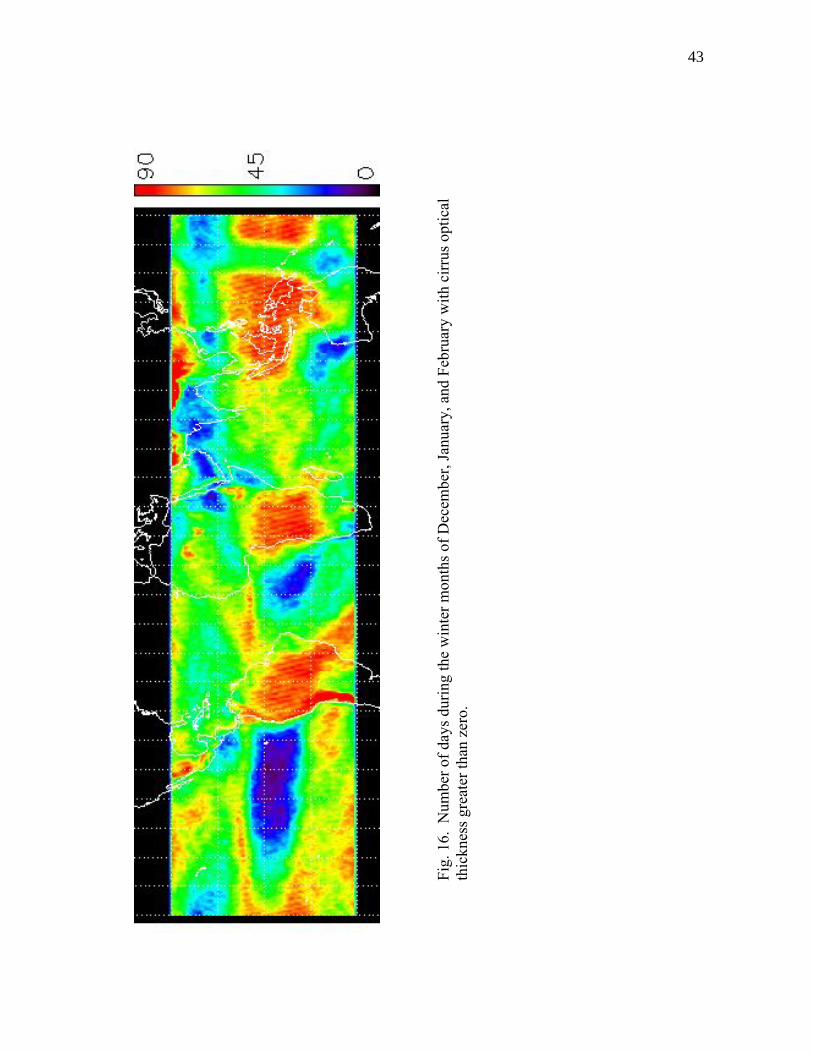
16 Number of days during the winter months of December, January,and February with cirrus optical thickness greater than zero……………… 43

17 Number of days during the summer months of June, July,and August with cirrus optical thickness greater than zero…………….….. 44

18 Sample AVIRIS images……………………………………………………. 48

19 A cirrus reflectance spectrum measured by AVIRIS………………………. 49

20 Mid-latitude cirrus phase functions………………………………………... 54

21 Sample look-up table for AVIRIS retrieval…………………………….….. 55

22 AVIRIS Scene 1 images…………………………………………………… 58

23 Scene 1 AVIRIS 1.38 vs. 1.24 µm scatter plot…………………………….. 59

24 Scene 1 retrieval images………………………………………………….... 60







1

1. INTRODUCTION

The knowledge of the optical properties (cloud optical thickness and ice crystal

effective size, in particular) of cirrus clouds is essential to the understanding of the

radiation balance and climate feedback associated with cirrus radiative forcing. Cirrus

clouds may substantially regulate the long-wave radiative energy exchange in the

vicinity of the tropical tropopause, and thus are radiatively important [17], [18]. Thin

cirrus clouds near the tropical tropopause occur frequently [47], [43], and have been

detected by satellite measurements [36], ground-based lidar [27], and space shuttle-

borne lidars [45]. Total cirrus cover has been found to be over 50% for the entire tropics

[5], and a thin cirrus layer may be present as much as 80% of the time in this region [42].

On a global scale, thin cirrus clouds are primarily confined to the tropical regions, with a

rather sharp frequency of presence over the Western Pacific Ocean, particularly during

the northern winter when the tropopause temperature is lowest [35], [21]. Most recently,

Dessler and Yang [7] showed that sub-visual cirrus clouds, with optical thickness less

than 0.03 [38], are ubiquitous over the tropics.

Cirrus clouds have been studied in some detail, and the general radiative and

microphysical properties of such clouds have been inferred and modeled in previous

studies [1], [2], [4], [5]. However, despite the facts that tropical cirrus clouds have a

significant impact on the local radiation budget and climate, and are ubiquitous near the

_______________This thesis follows the style and format of IEEE Transactions on Geoscience andRemote Sensing.

2

tropical tropopause (over the Western Pacific, in particular), relatively little is known

about their spatial and temporal distributions. Relevant studies are hampered by the lack

of detailed measurements of the radiative and microphysical properties of these clouds,

although recent studies have focused on this issue [30]. In fact, cirrus clouds are one of

the most uncertain components in atmospheric research because of their high altitudes,

optically thin nature, and the nonsphericity of ice crystals in those clouds.

Optical thickness of cirrus clouds is of major interest in the study of the radiative

effects of these clouds. Thick clouds reflect more short-wave radiation to space and trap

more long-wave radiation in the atmosphere than thin clouds. Also, ice clouds (i.e.,

cirrus) reflect and scatter radiation differently than water clouds. Even sub-visual cirrus

clouds (i.e., invisible to the naked eye) play a role in the radiation budget, although to

what extent is still unknown. An important factor in determining the optical thickness of

a cirrus cloud is the effective size of the ice crystals that compose such a cloud.

Following the principles of radiative scattering, larger ice crystals scatter more radiation

in the forward direction, whereas smaller crystals have less forward scattering and more

backscattering. These phenomena play a key role in determining the optical thickness of

the cloud. Thus, a significant amount of the current research efforts in the remote

sensing community have been focused on quantifying these radiative properties.

One instrument used in the study of cirrus clouds is the Airborne Visible Infrared

Imaging Spectrometer (AVIRIS) [40], [16]. The AVIRIS instrument, developed by the

NASA Jet Propulsion Laboratory, contiguously covers the spectral region from 0.4 to

2.5 µm, using 224 channels. When viewing from an ER-2 aircraft at an altitude of 20

3

km, the resolution is approximately 20 m × 20 m with a swath width of 12 km. The

spatial resolution can be increased even further (with a smaller swath width) at lower

altitudes. This instrument is useful in various field campaigns, as well as for data

validation. However, data from this instrument is limited to specific areas and times,

and does not have a global reach.

Of a somewhat greater importance to the research discussed here is the satellite-

borne Moderate-resolution Imaging Spectroradiometer (MODIS). MODIS has a much

more extensive view of the earth than does AVIRIS, although at a much lower spatial

resolution. It is equipped with 36 spectral bands, and was designed for the studies of the

atmosphere, land and ocean [22], [24], [34]. The MODIS instrument is currently a key

component of NASA’s Earth Observing System (EOS), as it is on board both the Terra

and Aqua satellites. From these satellites, at an altitude of 705 km, MODIS has a spatial

resolution of 1 km with a viewing swath of 2330 km, and can provide a global coverage

within 1 to 2 days. Data from this instrument is used extensively in the research

discussed here.

MODIS is the first satellite-borne instrument that features the 1.375 µm channel for

the exclusive study of cirrus clouds. The 1.375 µm channel is located in a strong water

vapor absorption band; therefore, the 1.375 µm reflectance included in the MODIS

level-1b calibrated radiance data set is due essentially to the reflection by high ice

clouds, which undergoes relatively little attenuation by the water vapor above these

clouds. Unlike the 1.375 µm channel, the solar radiation at a visible wavelength, say,

0.66 µm, is reflected by both low- and middle-level clouds composed of water droplets

4

as well as high clouds composed of ice crystals. For cirrus cloudy conditions, the

reflected solar radiation at a visible wavelength is strongly contaminated by the surface

reflection. Therefore, the measured 0.66 µm reflectance cannot be considered as the

reflectance of cirrus clouds. However, MODIS bands 1 (0.66 µm) and 26 (1.375 µm)

can be used together to obtain isolated cirrus reflectance at visible wavelengths (0.4 µm

< λ < 1.0 µm) [14]. This method is now an operational MODIS product. This derived

cirrus reflectance allows for the independent study of cirrus cloud optical properties.

The study presented here will consist of research devoted to the understanding of the

radiative properties of cirrus clouds, as well as the spatial and temporal distributions of

such clouds. A general methodology will first be described in Section 2. This section

also contains a brief overview of the science background required for the present study.

In Section 3, a new method is presented to convert MODIS isolated cirrus reflectance,

which is derived using the algorithm of Gao et al. [14], to the corresponding optical

thickness for tropical cirrus clouds. A brief survey of the tropical cirrus optical thickness

fields is then be presented in Section 4. Section 5 introduces a new method for

simultaneously retrieving cirrus cloud optical thickness and ice crystal effective diameter

from 1.38 and 1.88 µm reflectance. Finally, in Section 6, the conclusions are

summarized and discussed. It is hoped that this study helps to address several

unresolved issues in the field of atmospheric remote sensing.

5

2. METHODOLOGY

2.1 Research Objectives

The objectives of the research discussed here are three-fold:

• Cloud optical thickness of tropical cirrus is retrieved using the 0.66- and

1.375 µm MODIS level-1b calibrated radiance data and a simple look-up

table approach. All MODIS data are obtained from the data access system at

NASA Goddard DAAC.

• A preliminary global survey of tropical cirrus cover is performed using the

retrieval code produced in Objective 1. MODIS level-3 daily gridded cirrus

reflectance is converted into cirrus optical thickness, which is then compared

with the MODIS operational cloud product [24], [34].

• Cirrus optical thickness and ice crystal effective diameter are retrieved

simultaneously using AVIRIS 0.66, 1.38, and 1.88 µm reflectance

measurements and a simple look-up table approach. The AVIRIS data used

in the research presented here are obtained from Dr. Bo-Cai Gao at the Naval

Research Laboratory.

2.2 DISORT

The research presented here makes use of the Discrete Ordinates Radiative Transfer

(DISORT) model for reflectance calculations and look-up table generation. The

DISORT code is a numerical algorithm that models the scattering and emittance of

6

monochromatic radiation in a layered medium. It is capable of radiative calculations

involving wavelengths ranging from the ultraviolet to the microwave region of the

spectrum. The equations employed by DISORT are based on the well-known theory of

radiative transfer described by Chandrasekhar [3]. Here, we use the DISORT 2.0 Beta

algorithm for our calculations, which is available to the public and at the present time is

the most current version of the code developed by Stamnes et al. [39].

DISORT calculates the transfer of monochromatic radiation at frequency ν through a

plane-parallel medium using

µτ µ φτ

τ µ φ τ µ φν νν ν ν ν

du

du S

( , , )( , , ) ( , , )= − , (1)

where uν(τν,µ,φ) is the specific intensity in the (µ,φ) direction with optical thickness τν

(measured perpendicular to the medium surface), azimuthal angle φ, and cosine of the

polar angle µ. The source function Sν is given by

S d d P

u Q

ν νν ν

π

ν ν

ν ν ν ν

τ µ φω τ

πφ µ τ µ φ µ φ

τ µ φ τ µ φ

( , , )( )

( , , ; , )

( , , ) ( , , ),

= ′ ′ ′ ′

× ′ ′ +

∫ ∫−4 0

2

1

1

(2)

where ων(τν) is the single-scattering albedo and Pν(τν,µ,φ;µ′,φ′) is the phase function.

Qν(τν,µ,φ) is the internal source term, and is given by

Q Q Qthermal beamν ν ν ν ν ντ µ φ τ µ φ τ µ φ( , , ) ( , , ) ( , , )( ) ( )= + , (3)

Q B Tthermalν ν ν ν ντ µ φ ω τ( )( , , ) [ ( )] ( )= −1 , and (4)

7

Q I Pbeamν ν

ν νν ν

ν

τ µ φω τ

πτ µ φ µ φ

τµ

( )( , , )( )

( , , ; , )

exp ,

= −

×−

4 0 0 0

0

(5)

where Q thermalν ντ µ φ( )( , , ) is the source term for thermal emission in local thermodynamic

equilibrium, Q beamν ντ µ φ( )( , , ) is the source term for a parallel beam incident in direction

µ φ0 0, on a non-emitting medium under the usual diffuse-direct distinction, Bν(T) is the

Planck function at temperature T, and I0 is the incident intensity [39].

In the DISORT method, the scattering phase function is expanded in terms of

Legendre polynomials. Because the size of ice crystals is much larger than the

wavelength of solar radiation, the corresponding phase function is strongly peaked in the

forward direction. For a phase function with a strong forward peak, thousands of

Legendre polynomial terms are required in the phase function expansion. In practice,

the strong forward peak needs to be truncated, for example, by using the delta-M method

[46]. In this study, however, we use the δ-fit method [20], which is an extension of the

delta-M method. The δ-fit method uses a least-squares fitting approach to generate the

coefficients (cl) of the Legendre polynomial expansion. The objective is to minimize the

relative difference ε between the approximated phase function P′(θI) and the actual phase

function Pac(θI):

εθθ

=′

−

∑w

P

Pii

ac ii

( )( )

12

, (6)

8

′ ==

∑P c pi l l i

l

Nstr

( ) (cos )θ θ0

, (7)

where θI is the scattering angle, wi is the weight for each scattering angle, pl(cosθI) is

the lth Legendre polynomial, and Nstr is the number of streams (expansion terms)

needed for the desired accuracy.

The expansion coefficients cl are calculated by solving the least-squares fitting

problem ∂ε ∂ck = 0 (k=0,N):

p

Pw

c p

Pk i

ac ii

l l i

ac il

N

i

str

(cos )( )

(cos )( )

θθ

θθ

−

===

∑∑ 1 000

. (8)

The normalized phase function can then be written as

Pf

Pfit i iδ θ θ− =−

′( ) ( )1

1. (9)

For the studies described here, we use 32 streams to represent the phase function

(Nstr=32). The δ-fit method described here allows for a better estimation of the phase

function at large scattering angles than the conventional method [20].

2.3 MODIS Cirrus Reflectance

In this study, the optical thickness look-up library is generated under the assumption

of the presence of a single cirrus cloud in a completely transparent atmosphere with no

surface reflection. However, reflectance of the visible band contained in level-1b

calibrated radiance data from the MODIS instrument on board both the Terra and Aqua

9

satellites includes both atmospheric and surface effects (which include attenuation,

scattering, surface reflectance, etc.). The need arises then to remove these effects from

the data in order to match the conditions used in the look-up library.

The method used to remove surface and atmospheric effects from MODIS level 1b

data to obtain the “true” cirrus reflectance is described in Gao et al. [14]. First, the

atmosphere is assumed to be composed of three distinct layers. The top layer is

composed of the water vapor above cirrus clouds (which acts to attenuate both the

incoming and reflected radiation), the middle layer contains the cirrus clouds, and the

bottom layer consists of low-level water clouds, aerosols, water vapor (which accounts

for about 90-99% of the total atmospheric water vapor), and the surface. This bottom

layer is classified as the “virtual surface,” which takes into account the effects of

absorption and scattering by various gases, water vapor, aerosols below cirrus clouds,

and low- and mid-level clouds, as well as surface reflection. Fig. 1 shows the

atmospheric configuration assumed here. The “virtual surface,” or, more specifically,

the low-level water vapor, acts to absorb most, if not all, of the radiation transmitted

through cirrus clouds and surface reflected 1.375 µm radiation. Thus, its effects are

considered negligible in the MODIS measurement of 1.375 µm reflectance (i.e., the 1.38

µm reflectance can be considered as only that which is reflected by cirrus clouds). The

0.66 µm radiation, however, is in fact affected by the “virtual surface.” The radiation at

this wavelength is able to penetrate through the low-level water vapor, and is then

reflected by low-level water clouds and the surface of the earth. In effect, the 0.66 µm

10

Fig. 1. The atmospheric configuration assumed for the cirrus bi-directionalreflectance retrieval in Gao et al. (2002).

Surface

Low-level clouds, aerosols, andWater vapor (90-99%)

Cirrus and contrails

Water vapor (1-10%)

11

reflectance measured by MODIS includes the surface and water cloud reflectance, and

cannot be considered solely as the cirrus reflectance.

Previous studies have shown that the relationship between the 0.66 and 1.375 µm

cirrus reflectance (without atmospheric and surface effects) is quasi-linear [13], and has

a slope smaller than 1 due to weak ice crystal absorption of the 1.375 µm band. Fig. 2

illustrates this correlation using calculated data from DISORT for nine CEPEX size

distributions used in this study (these are discussed in Section 3.1.1). The slope of the

linear-fit line is indicated at the top of the figure. For MODIS data, cirrus reflectance is

coupled with the effects of the atmosphere and the surface. Gao et al. [14] show that the

apparent reflectances at MODIS bands 1 and 26 under cirrus cloudy condition are

correlated as follows:

r r d1 38 0 0 0 66 0 0. .( , , , ) ( , , , )µ φ µ φ µ φ µ φ= +Γ , (10)

where r1.375 and r0.66 are the apparent reflectances of the 1.375 and 0.66 µm bands,

respectively, Γ is the correlation between the 1.375 and. 0.66 µm band apparent

reflectance, and d depends on the optical properties of cirrus clouds and the absorption

and scattering by various gases, water vapor, aerosols below cirrus clouds, and low- and

mid-level clouds, as well as surface reflection. Fig. 3 conceptually illustrates the method

for deriving Γ. The isolated cirrus reflectance (without the contamination of surface

reflection and atmospheric effects) can then be obtained as follows:

rr

c, ..( , , , )

( , , , )0 66 0 0

1 38 0 0µ φ µ φµ φ µ φ

=Γ

. (11)

12

Fig. 2. Scatter plot of DISORT calculated 0.66 vs. 1.375 µm reflectance values,with linear curve fitting.

13

Fig. 3. Conceptual illustration of the method for deriving Γ.

r1.38

r0.66 r0.66

r1.38

0 0

Slope=Γ Slope=Γ

Data

Data

Over Ocean Over Land

14

Furthermore, the cirrus reflectance in the visible region has little spectral variation, that

is,

r rcλ µ φ µ φ µ φ µ φ( , , , ) ( , , , ), .0 0 0 66 0 0≅ , (12)

where 0 4 1. µ λ µm m< < . Therefore, the derivation of cirrus reflectance at visible

wavelengths reduces to the determination of the parameter Γ. An algorithm based on

MODIS level-1b calibrated band 1 and 26 radiance data has been developed to

determine Γ [14], and consequently, the cirrus visible reflectance.

Fig. 4 (a) shows a 0.66 µm MODIS reflectance image taken over southeastern Asia.

The surface and low-level water clouds are clearly visible in this image. Fig. 4 (b) is the

corresponding 1.375 µm MODIS reflectance image. Note the absence of the surface and

low-level water clouds. Fig. 4 (c) is the derived visible cirrus reflectance calculated

using the cirrus reflectance retrieval algorithm developed by Gao et al. [14]. Note the

similarities between Figs. 4 (b) and (c). The optical thickness retrieval algorithm from

Section 2.3 has been integrated into the cirrus reflectance algorithm. This combination

algorithm is capable of optical thickness retrieval using MODIS level-1b calibrated

radiance data on a pixel-by-pixel basis.

15

Fig. 4. Sample MODIS images illustrating the method of Gao et al. (a) 0.66µm channel MODIS image over southeastern Asia. (b) 1.375 µm channelMODIS image corresponding to (a). (c) Derived visible cirrus reflectancecorresponding to (a).

16

3. CIRRUS OPTICAL THICKNESS FROM MODIS LEVEL-1B

REFLECTANCE DATA*

3.1 Methodology

The general methodology used to retrieve the optical thickness of tropical cirrus

clouds from the MODIS 0.66-µm and 1.375-µm bands essentially follows the physical

principle shown by Nakajima and King [32], who found that the reflectance of clouds at

a visible channel is sensitive to cloud optical thickness and insensitive to cloud particle

size. In the present study, a cirrus optical property database is created first by integrating

the single scattering properties of individual ice crystal habits over in-situ observed size

distributions and the applicable spectral bands. A representative size distribution is then

chosen for the production of an optical thickness look-up table. This look-up table is

created using the Discrete Ordinates Radiative Transfer (DISORT) code [39] for an

isolated cirrus cloud without including atmospheric absorption. Furthermore, using the

algorithm developed by Gao et al. [14], isolated cirrus reflectance at visible wavelengths

is then derived by removing the atmospheric effects and surface reflection on the basis

of the correlation of MODIS level-1b calibrated band 1 (0.66 µm) and band 26 (1.375

µm) radiance data. Consequently, the optical thickness is derived from a look-up

interpolation based on the pre-calculated relationship between optical thickness and

cirrus reflectance.

_______________* 2004 IEEE. Reprinted, with permission, from K. Meyer, P. Yang, and B.-C. Gao, “Optical thicknessof tropical cirrus clouds derived from the MODIS 0.66- and 1.375-µm channels,” IEEE Trans. Geosci.Remote Sensing, 42, 2004.

17

3.1.1 Optical Properties Database

The scattering properties for the individual ice crystal habits used to create the

optical properties database are discussed in Yang et al. [49]. The scattering database

covers six habits, 56 wavelength channels (0.2-5.0 µm), and 24 size bins (3-4000 µm, in

terms of maximum crystal dimension). Tropical cirrus clouds are considered to contain

only three of these habits: rough aggregates, solid columns, and bullet rosettes. For the

bullet rosette data in this study, spatial bullet rosettes composed of two to six bullet

branches randomly oriented in space are used [48]. Intuitively, these three habits vary in

concentration from cloud to cloud. However, it is useful to approximate an average

habit percentage to describe tropical cirrus in general. The habit percentage used in this

study is assumed to be 33.7% solid columns, 24.7% bullet rosettes, and 41.6%

aggregates [29].

To integrate the scattering properties with respect to ice crystal size, in-situ

observational size distribution data are needed. Here, data obtained during the Central

Equatorial Pacific Ocean Experiment (CEPEX) are used. These data were collected

from three independent cirrus anvils on March 17, April 1, and April 4, 1993, using an

aircraft-borne Particle Measuring System (PMS) two-dimensional cloud probe (2DC)

and a video ice particle sampler (VIPS) [19], [28], [10].

Integration of cirrus optical properties is then completed over the nine CEPEX size

distributions using previously defined formulas [33]. Calculated properties of interest to

this study include the mean effective diameter, extinction coefficient, single-scattering

albedo, asymmetry factor, percentage of delta-transmission, truncation energy, and the

18

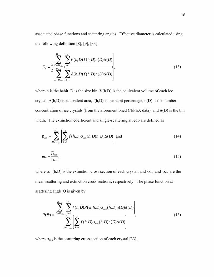
associated phase functions and scattering angles. Effective diameter is calculated using

the following definition [8], [9], [33]:

D

V h D f h D n D D

A h D f h D n D D

ehD D

D

hD D

D=

==

==

∑∑

∑∑32

1

3

1

3

( , ) ( , ) ( ) ( )

( , ) ( , ) ( ) ( )

,min

max

min

max

∆

∆

(13)

where h is the habit, D is the size bin, V(h,D) is the equivalent volume of each ice

crystal, A(h,D) is equivalent area, f(h,D) is the habit percentage, n(D) is the number

concentration of ice crystals (from the aforementioned CEPEX data), and ∆(D) is the bin

width. The extinction coefficient and single-scattering albedo are defined as

β σext ext

hD D

D

f h D h D n D D=

==

∑∑ ( , ) ( , ) ( ) ( )

min

max

∆1

3

and (14)

ωσσ

osca

ext

= , (15)

where σext(h,D) is the extinction cross section of each crystal, and σsca and σext are the

mean scattering and extinction cross sections, respectively. The phase function at

scattering angle Θ is given by

P

f h D P h D h D n D D

f h D h D n D D

sca

hD D

D

sca

hD D

D( )

( , ) ( , , ) ( , ) ( ) ( )

( , ) ( , ) ( ) ( )

,min

max

min

maxΘ

Θ ∆

∆

=

==

==

∑∑

∑∑

σ

σ

1

3

1

3(16)

where σsca is the scattering cross section of each crystal [33].

19

Fig. 5 shows the bulk scattering phase function at different effective sizes at

wavelengths 0.66 µm and 1.375 µm for tropical cirrus clouds (the different curves in the

plot indicate different size distributions, i.e. different effective sizes). The nine size

distributions of cirrus clouds in CEPEX (effective diameters ranging from 17.7 µm to

128.8 µm) were used in the figure. The habit and percentage of ice particles are

illustrated on the top of the figure. Evidently, the phase functions are strongly forward-

peaked. The 22° and 46° scattering maxima corresponding to halos are associated with

the hexagonal structure of the particles. The detailed features of the scattering phase

function and associated physical mechanisms can be found in Yang and Liou [48] and

Macke et al. [26].

3.1.2 Optical Thickness Look-up Library

In this study, the 0.66 µm visible band and the 1.375 µm “cirrus detection” band [13]

are used first to derive the isolated cirrus bi-directional reflectance (at visible

wavelengths) free of surface reflection and atmospheric effects [14]. To retrieve the

optical thickness of tropical cirrus clouds, a correlation between cirrus reflectance and

optical thickness must be established. This is accomplished using the DISORT code

20

Fig. 5. Phase function plots for the 0.66 and 1.375 µm wavelength channels.The habits used in this study are also shown above.

21

to model the radiative effects of an isolated cirrus cloud on the solar wavelengths of

interest. Scattering data from the previously calculated optical properties database is

used as input for each DISORT run. DISORT is first run using all nine tropical cirrus

cases (effective diameters ranging from 17.7 to 128.1 µm) for optical depths ranging

from 0.002 to 20.0. A limited number of viewing geometries (solar and viewing zenith

angles, and relative azimuth angles) are used for comparison purposes. This run allows

the determination of the correlation between the cirrus reflectance for each wavelength

and the optical thickness of the cloud.

Fig. 6 shows the correlation between 0.66 µm reflectance and optical thickness for

four independent viewing geometries. Reflectance of the 0.66 µm wavelength is found to

be quite sensitive to the optical thickness of the cloud, but is not sensitive to ice crystal

size because of the negligible absorption of ice at this wavelength, as evident from the

refractive index of ice [44]. It is therefore possible to retrieve the optical depth of a

given tropical cirrus cloud by using the cirrus reflectance at the 0.66 µm wavelength

channel. The relatively small reflectance deviation between the smallest and largest

effective diameters in Fig. 6 indicates little sensitivity to crystal size. With these results,

a single CEPEX size distribution can be selected to use as a representative case to

generate the look-up library. For this study, the median size distribution (De = 34.97

µm) has been chosen.

22

Fig. 6. Plot of 0.66 µm reflectance vs. optical thickness from DISORTcalculations (effective diameters from 17.7 µm to 128.1 µm).

23

The DISORT code is run using 4864 solar and satellite viewing geometries, with solar

and viewing zenith angles from 0 to 75o (five degree intervals), and relative azimuth

angles from 0 to 180o (ten degree intervals). Input optical depths range from 0.002 to

100.0 (optical depths between 0.0 and 0.002 are assumed to have a linear relationship

with the corresponding 0.66 µm reflectance values, allowing for the retrieval of sub-

visual cirrus). The resulting look-up library consists of the 0.66 µm cirrus reflectance

and the optical depths for each solar and satellite-view geometry used in the retrieval.

An algorithm has been developed to interpolate the optical thickness of a given cirrus

cloud from the look-up library using only the solar and view zenith angle, the relative

azimuth angle, and the corresponding 0.66 µm cirrus reflectance value as input.

3.2 Optical Thickness Retrieval from MODIS Data

To demonstrate the effectiveness of the algorithm and methods discussed in Section

3.1, we apply the cirrus reflectance and optical thickness retrieval algorithm to MODIS

data from the Terra satellite. Here, the publicly available 0.66 and 1.375 µm (MODIS

channels 1 and 26, respectively) level-1b calibrated radiance data are used. These data

have 1 km spatial resolution, and have been processed to sensor units and are

radiometrically corrected and geolocated. A normal granule of MODIS level-1b data

has a size of 1354 × 2030 pixels. Due to the shape of the earth as well as the orientation

of the beam swath, individual pixel size varies throughout the granule. Pixels at nadir in

the MODIS granule are generally square in shape, while pixels at the “eastern” and

24

“western” sides are not square and are larger in size. However, this irregularity does not

affect the retrieval of optical thickness in this study.

The retrieval algorithm has been developed to first retrieve the isolated visible cirrus

reflectance for a single MODIS granule. The optical thickness is then interpolated from

the reflectance data and the optical thickness look-up table. The algorithm itself is

written to interpolate the optical thickness at each individual pixel in the MODIS granule

(2748620 total pixels per granule). Intuitively, this is extremely CPU intensive (it takes

more than 15 minutes to complete the retrieval for a single MODIS granule on a

workstation). However, this approach has the ability to retrieve the optical thickness of

tropical cirrus clouds (including those which are optically thin, and are thus invisible) in

great detail.

In this study, the retrieval algorithm has been applied to two individual MODIS

granules to demonstrate its flexibility: one over the ocean and the other over land. Fig.

7 (a) is a visible MODIS image (using the 0.66 µm wavelength channel) from the Terra

satellite over the Indian Ocean on July 13, 2002. Low-level water clouds are prevalent

throughout the image, most notably on the bottom and right sides. Scattered cumulus

lines are also visible. However, blow-off cirrus clouds are clearly visible in the central

regions. For this granule, this region of blow-off cirrus is the area of focus for the

retrieval.

25

Fig. 7. Terra MODIS level-1b image over the Indian Ocean (July 13, 2003).(a) Visible MODIS image (0.66 µm channel). (b) 1.375 µm channel imagecorresponding to (a). The white outline indicates the region of optical thicknessretrieval.

26

Fig. 8. Retrieved optical thickness of the outlined region in Fig. 7 (b). Note thesensitivity to optically thin cirrus clouds.

27

Fig. 7 (b) is the 1.375 µm “cirrus” channel image. This image allows for a better

view of the spatial extent of cirrus cover in the granule. Clearly, cirrus clouds cover a

large portion of this granule, with the possibility of sub-visual cirrus in some regions.

The white outline in this image denotes the region of optical thickness retrieval. The

selected region has a size of 301 × 401 pixels. Notice the relatively low reflectance of

cirrus clouds within this region, indicating the possible presence of optically thin cirrus.

Fig. 8 shows the retrieved optical thickness of the selected region in Fig. 7 (b).

Plotted optical thickness values range from 0.0 to 3.0, as indicated by the bar on the

right-hand side. The physical features of the cirrus layer are clearly visible in this image.

Also, notice the sensitivity to small optical thickness values in this image (darker shades

of blue and purple). These small values indicate the presence of optically thin cirrus.

The second granule used in this study is one over land. Fig. 9 (a) is a visible MODIS

image (again using the 0.66 µm wavelength channel) taken over the continent of Africa

at 9:25 UTC on January 30, 2003, from the Terra satellite. Surface features are clearly

visible in the image (notably in the upper regions of the image). There is also a large

presence of convective clouds in the southern portions of the image. On the northern

edge of this convection, in the central region of the image, is a small area of thin blow-

off cirrus. The retrieval will focus on this region of the granule.

28

Fig. 9. Terra MODIS level-1b image over Africa (January 30, 2003). (a)Visible MODIS image (0.66 µm channel). Note the surface features evident inthe upper region of the image. (b) 1.375 µm wavelength image correspondingto (a). The white outline indicates the region of optical thickness retrieval.

29

Fig. 10. Retrieved optical thickness of the outlined region in Fig. 9 (b). Notethe sensitivity to optically thin cirrus clouds.

30

Fig. 9 (b) is the corresponding 1.375 µm “cirrus” image. The surface effects and

low-level water clouds are now removed. Thick cirrus layers are evident over the

regions of convection, while thin blow-off cirrus layers are visible over the center of the

image. Again, the white outlined box in this plot indicates the region of optical

thickness retrieval. Like the previous granule, this region has a size in pixels of 301 ×

401.

Fig. 10 shows the retrieved optical thickness of the selected region. Plotted optical

thickness values range from 0.0 to 3.0, as indicated by the bar on the right-hand side.

Similar to Fig. 8, notice the sensitivity to small values of optical thickness (again, the

darker shades of blue and purple). The physical features of the layer are strikingly

visible in this image, with the thin, wispy nature of cirrus clouds clearly evident. This

image, as well as Fig. 8, illustrates the ability of the algorithm to retrieve the optical

thickness of sub-visual cirrus.

As previously stated, our algorithm is complementary to the standard cloud retrieval

algorithm [23], [34], which has been implemented as one of the MODIS operational data

products. The MODIS operational cloud retrieval algorithm retrieves the optical

thickness of all cloud cover observed by MODIS. Using the present algorithm to

retrieve the optical thickness of cirrus clouds, it is possible to remove these clouds to

obtain the optical thickness of underlying water clouds. This is illustrated in Figs. 11

and 12. Fig. 11 (a) is a 0.66 µm MODIS image over the western equatorial Pacific

Ocean on February 6, 2003. Notice the overlay of thin cirrus over low-level convective

clouds in the central region of the image. Fig. 11 (b), the corresponding 1.375 µm

31

Fig. 11. Terra MODIS level-1b image over the western equatorial PacificOcean (February 6, 2003). (a) Visible MODIS image (0.66 µm channel). (b)1.375 µm wavelength image corresponding to (a). The white outline indicatesthe region of optical thickness retrieval.

32

Fig. 12. Retrieved optical thickness images from outlined region in Fig. 11 (b).(a) MODIS operational cloud retrieval algorithm optical thickness image of theoutlined region in Fig. 11 (b). (b) Corresponding optical thickness image fromthe cirrus optical thickness retrieval algorithm. (c) Difference between (a) and(b). Note the absence of high-level cirrus in (c).

33

image, shows the cirrus cover in more detail. Again, the white outlined box indicates the

region of interest.

Figs. 12 (a) and (b) show the retrieved optical thickness from the MODIS operational

cloud retrieval algorithm [24], [34] and the present cirrus optical thickness retrieval

algorithm, respectively. Similar to Fig. 11 (a), the high-level cirrus overlay is clearly

visible in Fig. 12 (a). Fig. 12 (b) can now be subtracted from Fig. 12 (a) to obtain the

low-level water cloud optical depth image. In Fig. 12 (c), high-level cirrus has been

removed, revealing the optical thickness of the underlying water clouds.

3.3 Discussion/Summary

In this study, an algorithm was developed to retrieve the optical thickness of tropical

cirrus clouds using cirrus visible reflectance derived from MODIS bands 1 and 26,

which are publicly available. An optical properties database consisting of the mean

scattering and absorption properties of several different ice crystal habits for various

experimentally measured size distributions using previously calculated scattering and

optical properties data [49] was first constructed. The Discrete Ordinates Radiative

Transfer (DISORT) code was then used to establish a correlation between tropical cirrus

reflectance and cloud optical thickness. Data from the optical properties database were

used for these DISORT calculations. All atmospheric and surface effects were assumed

to be negligible in these calculations. Reflectance of 0.66 µm radiation by cirrus clouds

is sensitive only to cirrus optical thickness. It is therefore possible to retrieve the optical

thickness of tropical cirrus clouds, given the satellite viewing geometry and the 0.66 µm

34

reflectance values. An optical thickness look-up library was then created consisting of

data from a “representative” tropical cirrus size distribution, in this case the median of

the nine CEPEX size distributions.

An algorithm was then developed to retrieve the optical thickness of tropical cirrus

using MODIS level-1b radiance data. Atmospheric and surface effects are removed

from the data using the cirrus reflectance retrieval algorithm. The optical thickness

retrieval algorithm was then integrated into the cirrus reflectance algorithm. It should be

noted that the present algorithm is not an operational algorithm. It has been developed

to compliment the aforementioned MODIS cloud retrieval algorithm (currently

implemented as one of the MODIS operational data products) for the case of cirrus

clouds. This approach is especially effective for isolated cirrus clouds, but is also

effective for the case of cirrus over water clouds, or cloud overlap. This is illustrated

using calibrated reflectance data from the MODIS instrument on board the Terra

satellite.

35

4. SURVEY OF TROPICAL CIRRUS OPTICAL THICKNESS

USING MODIS LEVEL-3 DATA

In order to understand the effects of cirrus clouds on the earth’s radiative processes

and climate system, a good knowledge of the nature, spatial extent, location, and

frequency of occurrence of such clouds is needed. With the development of MODIS and

the subsequent inclusion of the 1.375 µm “cirrus detection” channel, an unprecedented

global view of cirrus cloud cover is now possible. As an extension of Section 3, a

preliminary survey of the optical thickness fields of tropical cirrus clouds has been

undertaken. This includes the extent of cirrus cover in the tropics, as well as frequency

of occurrence.

4.1 Methodology

The general methodology for the preliminary study of tropical cirrus cloud optical

thickness is fairly straightforward. Cloud optical thickness is first retrieved from

MODIS level-3 daily gridded atmospheric data, which are available to the public. These

data contain daily mean cirrus reflectance values, relative azimuth angles, and solar and

viewing zenith angles. For the retrieval, the tropical cirrus optical thickness retrieval

algorithm from Section 3 is modified to accept level-3 data as input. The daily mean

tropical cirrus optical thickness is retrieved for each calendar day. Analyses of tropical

cirrus cover can then be completed.

36

4.2 Retrieval

4.2.1 MODIS Level-3 Daily Gridded Data

MODIS level-3 daily gridded atmospheric data are a global product. They contain

over 500 statistically averaged atmospheric parameters at a 1 degree by 1 degree spatial

resolution. All level-3 atmospheric parameters are derived from four level-2 MODIS

atmospheric products (Aerosol, Water Vapor, Cloud, and Atmosphere Profile). These

parameters are averaged over a 1 degree by 1 degree grid spacing for a 24-hour time

period (0000 to 2400 GMT), producing a daily 360 by 180 pixel grid as output. They

include actual atmospheric values, as well as standard deviations, quality assurance

weighted means and other statistically derived quantities for each parameter. Of these

parameters, isolated cirrus reflectance, derived from the operational algorithm of Gao et

al. [14], and the corresponding solar/satellite view geometries are of importance to the

present study. Level-3 daily gridded atmospheric data, from February 2000 to the

present, are publicly available through the NASA Distributed Active Archive Center

(DAAC). These data will be used as input to a modified tropical cirrus optical thickness

retrieval algorithm.

4.2.2 Tropical Cirrus Optical Thickness Retrieval Algorithm

The retrieval algorithm described in Section 3 is used in the present study to retrieve

the optical thickness of tropical cirrus clouds using MODIS level-3 daily gridded data.

This algorithm, however, is written to operate on MODIS level-1b data. A modified

version of the algorithm is therefore necessary for the retrieval described here.

37

Level-1b data is regional in scope and has a pixel resolution of 1354 × 2030 (1 km

by 1 km grid). As described above, MODIS level-3 data is global in scale with a pixel

resolution of 360 × 180. The algorithm’s input pixel resolution is reduced to the level-3

resolution. In addition, level-1b data contain raw reflectance values, and therefore the

isolated cirrus reflectance must be derived in the retrieval algorithm using the method of

Gao et al. [14]. Level-3 data, however, contain operationally derived isolated cirrus

reflectance. Therefore, the cirrus reflectance algorithm is removed from the optical

thickness retrieval code. Derived cirrus reflectance, as well as the solar/sensor zenith

angles and relative azimuth angles, are directly input into the retrieval code. Optical

thickness retrieval then follows the same method described in Section 3.

4.3 Preliminary Results

For the present study, the retrieval code has been run on fourteen consecutive months

of MODIS level-3 data. These data are from the Terra satellite, and cover the months

from September 2001 to October 2002. Only data between 30o N and 30o S are

considered. Derived isolated cirrus reflectance values and solar/satellite view geometry

data have been extracted and stored in daily data files. These files serve as input for the

retrieval code. It should be noted that, since only just over a year of data is used, the

results discussed here are not statistically sound. However, they do provide a glimpse of

the many studies that can be performed using this method.

38

Fig.

13.

MO

DIS

leve

l-3

deri

ved

isol

ated

cir

rus

refl

ecta

nce

from

Ter

ra s

atel

lite

on J

uly

27, 2

002.

39

Fig.

14.

Tro

pica

l cir

rus

optic

al th

ickn

ess

deri

ved

from

MO

DIS

leve

l-3

cirr

us r

efle

ctan

ce c

orre

spon

ding

to F

ig.

13.

40

Fig. 13 shows a sample MODIS level-3 mean cirrus reflectance image from the

Terra satellite for July 27, 2002. Cirrus reflectance values are scaled between 0.0 and

0.5, as indicated by the bar on the right-hand side. Most of the cirrus in this image

appears to be due to convective storms along the Intertropical Convergence Zone

(ITCZ), which is visible in a line of convection just north of the equator. High

reflectance values in this image indicate relatively thick cirrus clouds. Note the

concentration of cirrus over the western equatorial Pacific Ocean. This region

experiences relatively frequent convection, especially during the summer monsoon.

Fig. 14 shows the derived cirrus optical thickness plot corresponding to the image in

Fig. 13. Optical thickness values are scaled between 0.0 and 3.0, as indicated by the bar

on the right-hand side. This image appears very similar to Fig. 13, as is expected.

Again, the ITCZ is clearly visible just north of the equator. Note that the areas of large

optical thickness in this figure correspond to the areas of high cirrus reflectance in Fig.

13.

Fig. 15 shows the total number of days with cirrus optical thickness greater than zero

for the entire 14-month period between September 2001 and October 2002. This image

is scaled from 0 to 400 days, as indicated by the bar on the right-hand side. The ITCZ

appears as a thin band just north of the equator, except over Indonesia, where it widens

significantly. Note the relatively high frequency of cirrus cover over mountainous areas

such as the Andes in South America, the Himalayas in southern Asia, and to a lesser

extent the Sierra Madre Occidental and Sierra Madre Del Sur in the western portions of

Mexico. These patterns can be attributed to large-scale orographical lifting in these

41

regions. Also note the relatively high frequency of cirrus over the western equatorial

Pacific Ocean (particularly over Indonesia). This can be attributed to the frequent

convection experienced over this region.

Fig. 16 shows the number of days with cirrus optical thickness greater than zero

during the winter months of December 2001, and January and February 2002. This

image is scaled from 0 to 90 days, as indicated by the bar on the right-hand side. Note

that regions of highest cirrus frequency are located over large landmasses (e.g., South

America, southern Africa) and the islands of Indonesia. As expected, these regions are

also slightly south of the equator, due to the southern hemisphere summer and

subsequent southward movement of the ITCZ. Also, the aforementioned mountainous

areas are evident in this image.

Fig. 17 shows the number of days with cirrus optical thickness greater than zero

during the summer months of June, July, and August 2002. This image is scaled

between 0 and 90 days, as indicated by the bar on the right-hand side. A more

continuous and defined ITCZ is clearly evident in this image. Note the northward

movement of the regions of highest cirrus frequency, especially those over large

landmasses, which is due to the northern hemisphere summer. Also, note the

significantly large area of high frequency of cirrus occurrence over southern Asia,

undoubtedly due to the summer monsoons in this region.

42

Fig.

15.

Tot

al n

umbe

r of

day

s be

twee

n Se

ptem

ber

2001

and

Oct

ober

200

2 w

ith c

irru

s op

tical

thic

knes

s gr

eate

rth

an z

ero.

43

Fig.

16.

Num

ber

of d

ays

duri

ng th

e w

inte

r m

onth

s of

Dec

embe

r, J

anua

ry, a

nd F

ebru

ary

with

cir

rus

optic

alth

ickn

ess

grea

ter

than

zer

o.

44

Fig.

17.

Num

ber

of d

ays

duri

ng th

e su

mm

er m

onth

s of

Jun

e, J

uly,

and

Aug

ust w

ith c

irru

s op

tical

thic

knes

sgr

eate

r th

an z

ero.

45


The tropical cirrus optical thickness algorithm discussed in Section 3, when applied

to MODIS level-3 daily gridded data, can provide an impressive view of cirrus cover in

the tropics. While the preliminary results discussed here should not be considered a

sound statistical study, they do offer a glimpse of possible future endeavors using

MODIS level-3 daily gridded data with the optical thickness retrieval algorithm. A more

in depth analysis, taking into consideration meteorological processes and geographical

effects, can provide a more accurate study of tropical cirrus optical thickness fields.

46

5. CIRRUS OPTICAL THICKNESS AND EFFECTIVE SIZE FROM

AVIRIS DATA*

5.1 Background

5.1.1 The AVIRIS Instrument

AVIRIS (Airborne Visible Infrared Imaging Spectrometer) is a hyperspectral

imaging instrument designed and built at the Jet Propulsion Laboratory [40], [16]. The

imaging data acquired with AVIRIS have been used in a variety of research and

applications, including geology, agriculture, forestry, coastal and inland water studies,

environment hazards assessment, and urban studies [6]. AVIRIS is now an operational

instrument with reliable radiometric and spectral calibrations. It is equipped to view 224

narrow channels with widths of approximately 10 nm, covering the contiguous solar

spectral region between 0.4 and 2.5 µm. AVIRIS typically acquires images with a pixel

size of 20 m from a NASA ER-2 aircraft at an altitude of 20 km. The swath width on the

ground is approximately 12 km. AVIRIS can also acquire images from a low-altitude

aircraft at spatial resolutions of 1 to 4 m with reduced swath widths.

5.1.2 Cirrus Detections

Previously, it was reported [11], [12] that narrow channels near the centers of the

1.38 and 1.88 µm strong water vapor absorption bands are very effective in detecting

_______________*This work has been submitted to the IEEE for possible publication.

47

thin cirrus clouds based on the analysis of AVIRIS data collected in the late 1980s and

early 1990s. The mechanisms for cirrus detection are relatively simple. In the absence

of cirrus clouds, these narrow channels receive little solar radiance scattered by the

surface and low-level water clouds because of the strong absorption of solar radiation by

atmospheric water vapor located above them. When high-level cirrus clouds are present,

these channels receive solar radiances scattered by cirrus clouds that contrast well on the

dark background.

During the mid-1990s, a major upgrade to the AVIRIS instrument was made. The

signal to noise ratios of AVIRIS data improved significantly. Here, the newer AVIRIS

data sets are preferred to demonstrate again the capability of cirrus detections with

narrow channels near 1.38 and 1.88 µm. Fig. 18 (a) shows a true color AVIRIS image

(red: 0.66 µm; green: 0.55 µm; blue: 0.47 µm) acquired over Bowie, Maryland, near a

latitude of approximately 38.97°N and a longitude of approximately 76.74°W on July 7,

1996. Surface features are seen through the partially transparent thin cirrus clouds.

Figs. 18 (b) and 18 (c) show the 1.38-µm image and the 1.88-µm image, respectively.

Both channels allow for the detection of thin cirrus clouds.

5.1.3 Cirrus Reflectance Properties

In order to illustrate the reflectance properties of cirrus clouds, Fig. 19 shows an

“apparent reflectance” spectrum measured over an area covered by cirrus clouds above

Monterey Bay, California, on September 4, 1992. Omitting for convenience the

48

Fig. 18. Sample AVIRIS images. (a) A true color AVIRIS image (red: 0.66µm; green: 0.55 µm; blue: 0.47 µm), (b) the 1.38-µm channel image, and (c) the1.88-µm channel image processed from the AVIRIS data acquired over Bowiein Maryland near a latitude of approximately 38.97°N and a longitude of about76.74°W on July 7, 1996. Surface features are seen in (a), and thin cirrus cloudsare seen in (b) and (c).

49

Fig. 19. A cirrus reflectance spectrum measured by AVIRIS. Taken over anarea above Monterey Bay, California, on September 4, 1992. Also anatmospheric gas transmittance spectrum and an ice transmittance spectrum.

50

wavelength (l) and cosine-solar-zenith-angle (m0) dependencies, the “apparent

reflectance” at the aircraft or satellite is denoted as

r* = p L / (m0 E

0), (17)

where L is the radiance measured by the satellite and E0 is the extra-terrestrial solar

flux. The cirrus spectrum was scaled to 0.7 near 0.5 µm in order to avoid the

overlapping of this curve with the other two curves in the plot. The absorption features

of the atmospheric oxygen band centered near 0.76 µm, water vapor bands near 0.94,

1.13, 1.38, and 1.88 µm, and a carbon dioxide band near 2.06 µm are seen in this

spectrum. These features are the result of absorption by atmospheric gases located

above and within cirrus clouds. The solar radiation transmitted through cirrus clouds in

the downward path is mostly absorbed by atmospheric gases below cirrus and by liquid

water in the ocean. The ice absorption bands centered near 1.5 µm and 2.0 µm are also

seen. These bands are resulted from absorption by ice particles within cirrus clouds. In

order to help identify various absorption features contained in the cirrus spectrum, an

atmospheric gas transmittance spectrum and an ice transmittance spectrum (0.007 cm

thick) are also shown. Weak ice absorption occurs near 1.24 and 1.38 µm. The effects at

both wavelengths are expected to be about the same, since the imaginary parts of the ice

refractive index [25] are comparable.

The positions and widths of five MODIS visible and near-IR atmospheric window

channels used in the operational retrievals of MODIS cloud optical properties [24], [34]

and the 1.375-µm cirrus detecting channel are shown in thick horizontal bars above the

51

transmittance spectra in Fig. 19. A narrow channel centered near 1.88 µm with a width

of 30 nm, which is absent in any of the current or near-future meteorological satellite

sensors for cirrus detections, is also illustrated with a thinner horizontal bar in the lower

right portion of the plot. From the ice transmittance spectrum and cirrus reflectance

spectrum, it is seen that the ice absorption effect over the bandpass of the 1.375 µm

channel is weak, while the absorption effect over the bandpass of the 1.88 µm channel is

stronger. This difference allows, in principle, the simultaneous retrieval of optical

depths and ice particle size distributions using both channels with little contamination

from the surface or lower level water clouds (see Figs. 18 (b) and 18 (c)). Because the

two channels are located within water vapor absorption regions (see the cirrus

reflectance spectrum and gas transmittance spectrum), the water vapor absorption effects

must be properly modeled and removed before the two channels can be used for the

quantitative retrieval of cirrus optical properties.

5.2 Method

An empirical technique for estimating water vapor transmittances was previously

described in detail [13]. Over water surfaces, the scatter plot of the 1.375 µm channel

apparent reflectance values (r*1.375) versus the 1.24 µm channel apparent reflectance

values (r*1.24) is made. The slope of an empirically established line is estimated [13],

and this slope is considered to be the water vapor transmittance (T1.375) for the 1.375 µm

channel. Over land surfaces, the water vapor transmittance for the 1.375 µm channel is

similarly derived, except that the 0.66 µm channel is used in place of the 1.24 µm

52

channel . Because the ice particle absorption effect near 1.375 µm is weak, the intrinsic

cirrus reflectance for the 1.375 µm channel, r1.375, is approximately equal to the ratio of

r*1.375/ T1.375. This intrinsic reflectance is related to the cirrus optical depth [31].

For the 1.88 µm channel, both the atmospheric water vapor absorption effect and the

ice particle absorption effect are significant (see Fig. 19). The 1.88 µm channel water

vapor transmittance, T1.88, is predicted using the estimated 1.375 µm channel water

vapor transmittance, T1.375, and a line-by-line atmospheric transmittance code. The

HITRAN2000 line database [37] is used in the line-by-line calculations. The intrinsic

cirrus reflectance for the 1.88 µm channel, r1.88, is equal to the ratio of r*1.88/ T1.88. This

intrinsic reflectance is related to both the cirrus optical depth and the ice particle size

distributions.

After obtaining the intrinsic cirrus reflectances for both the 1.375 and 1.88 µm

channels, the retrieval of cirrus optical depth and ice particle size can be made using the

well established Nakajima and King [32] approach. In order to do so, look-up tables for

each sun/satellite viewing geometry (i.e., relative azimuth angle, as well as solar and

viewing zenith angles) must first be generated. Each look-up table should include the

1.38 and 1.88 µm reflectance values, along with the corresponding optical thickness and

effective diameter values. The Discrete Ordinates Radiative Transfer (DISORT) code

[39] is used for all radiance calculations under the assumption of isolated cirrus clouds

with no atmosphere above and below the clouds. This assumption is justified because

the Rayleigh scattering effects for wavelengths greater than about 1 µm are negligible.

53

Cirrus scattering properties (used as input for DISORT) are averaged from the results of

Yang et al. [49].

Fig. 20 shows the single-scattering phase functions for both the 1.38 and 1.88 µm

channels averaged from Yang [49]. The eight mid-latitude size distributions used in the

DISORT-generated look-up tables are shown in this plot, with effective diameters

ranging from 9.2 to 146.1 µm. The assumed habit percentages are shown in the 1.38 µm

plot. For effective diameters less than 70 µm, a habit percentage of 50% bullet rosettes,

25% plates, and 25% columns is assumed. For diameters greater than 70 µm, a

composition of 30% rough aggregates, 30% bullet rosettes, 20% columns, and 20%

plates is assumed [1].

Fig. 21 (a) shows a sample look-up table generated for one case study of AVIRIS

data (236.41o relative azimuth, 44.34o solar zenith, and nadir viewing zenith). Lines of

constant ice crystal effective diameter and cirrus optical thickness are labeled. Note the

sensitivity of the 1.38 µm wavelength to optical thickness, and the sensitivity of the 1.88

µm wavelength to effective diameter. For a given pair of intrinsic reflectance values of

the 1.38 and 1.88 µm channels, simultaneous retrievals of the optical thickness and ice

crystal size distribution can, in principle, be made using the simulated lookup table and a

simple table-searching procedure. Fig. 21 (b) shows a close-up of Fig. 21 (a), with

AVIRIS data superposed. The data used in this image are from the natural cirrus image

(Scene 3) described below.

54

Fig. 20. Mid-latitude cirrus phase functions. (a) Scattering phase function plotfor the 1.38 µm channel. (b) Scattering phase function plot for the 1.88 µmchannel. The habit percentage used in this study is shown in the 1.38 µm plot.

55

Fig. 21. Sample look-up table for AVIRIS retrieval. (a) Sample look-up tablefor the natural cirrus shown in Scene 3 (236.41o relative azimuth, 44.34o solarzenith, and nadir viewing zenith). (b) Close-up of (a) with Scene 3 AVIRISdata superposed.

56

5.3 Preliminary Results

The method described in Section III has been applied to three sets of AVIRIS data,

one containing aircraft-induced contrail cirrus (Scene 1) and two containing natural

cirrus (Scenes 2 and 3). Scenes 1 and 2 were taken over the coastal areas of New Jersey

on July 12, 1998 during the Long-term Ecosystem Observatory in 15 meters (LEO-15)

experiment [41]. LEO-15 was primarily designed for the study of shallow coastal

waters. Scene 3 was taken over Monterey Bay, California on September 4, 1992. The

cirrus-contaminated AVIRIS data is used for the research on simultaneous retrievals of

optical depths and ice particle size distributions. The preliminary retrieval results from

the three AVIRIS data sets are described below.

5.3.1 Contrail Cirrus (Scene 1)

Fig. 22 (a) shows the 1.24 µm channel image for the scene containing contrail cirrus.

The image covers an area of about 12 km by 10 km. It has 614 pixels from left to right

and 512 pixels from top to bottom. Most of the scene is covered by water, and only a

small fraction of the scene is covered by land. The center of the image is located at

approximately 39.47°N and 76.25°W. Small white dots are seen throughout the image.

These dots represent the wakes of boats in the water. The contrail itself is very thin

(very small reflectance), and stretches from left to right across the image. Fig. 22 (b) is

the 1.38 µm channel image. The contrail cirrus is clearly seen. The boat wakes

disappear in this image due to strong absorption by water vapor below the contrail cirrus.

Fig. 22 (c) shows the 1.88 µm image. It is almost identical to the image in Fig. 22 (b)

57

with the exception that the reflectance values are smaller than those of the 1.38 µm

channel.

Fig. 23 shows the scatter plot of the 1.38 µm channel apparent reflectance values

(r*1.375) versus the 1.24 µm channel apparent reflectance values (r*1.24) for the scene in

Fig. 22. The lower portion of the plot contains land pixels with larger 1.24 µm

reflectance values. Pixels covered by the contrail cirrus over the dark water surfaces are

clustered around a steep line at left, which has a slope of about 0.8. This slope is the

estimate of the water vapor transmittance (T1.375) for the 1.375 µm channel. The

derivations of the intrinsic cirrus reflectance values for the 1.375 µm channel (r1.375) and

the 1.88 µm channel (r1.88) are subsequently made using the techniques outlined in

Section 5.2. In order to improve the signal to noise ratios of the intrinsic cirrus

reflectances (r1.375 and r1.88), a spatial averaging of the data is performed. The resulting

data set has only 76 x 64 pixels.

During the practical retrieval process, the retrieval code has been written for each set

of AVIRIS image data using the computed scene-specific look-up table. The look-up

table resolution is doubled four times (from 8 effective diameters and 17 optical depths

to 113 effective diameters and 273 optical depths) using linear averaging. A simple

averaging of the optical thickness and effective diameters of the four nearest look-up

table points to each data pixel (effectively a data “box”) is performed.

58

Fig. 22. AVIRIS Scene 1 images. (a) 1.24 µm image for Scene 1. (b) 1.38 µmimage for Scene 1. (c) 1.88 µm image for Scene 1.

59

Fig. 23. Scene 1 AVIRIS 1.38 vs. 1.24 µm scatter plot. Note the horizontalswath of data points at the bottom of the plot, corresponding to low-level waterclouds and surface effects. The steep, narrow swath of points on the left side ofthe plot indicates cirrus clouds.

60

Fig. 24. Scene 1 retrieval images. (a) Retrieved cloud optical thicknesscorresponding to the images in Fig. 22. (b) Retrieved ice crystal effectivediameter corresponding to Fig. 22.

61

Fig. 24 (a) shows the retrieved cloud optical thickness of the scene in Fig. 22. The plot

range is scaled from 0.0 to 0.4, as displayed on the color bar. The retrieved optical

thickness values indicate the very thin nature of this contrail cirrus cloud. The overall

pattern of the image clearly matches that of Figs. 22 (a), 22 (b), and 22 (c). As expected,

the largest values of optical thickness are found in the middle portion of the contrail

cirrus.

Fig. 24 (b) shows the retrieved ice crystal effective diameter of the scene in Fig. 22.

The plot range is scaled from 0.0 to 110.0 µm. Again, the overall pattern of the image

clearly matches that of Figs. 22 (a), 22 (b), and 22 (c). The smallest ice crystal sizes are

generally found in the middle of the contrail cirrus (corresponding to large optical

thickness values). This is due to a unique aspect of 1.88 µm channel reflectance in that

smaller ice crystals reflect more radiation than larger ice crystals, as evidenced by the

plot in Fig. 21 (b).

5.3.2 Natural Cirrus (Scenes 2 and 3)

Fig. 25 (a) shows the 1.24 µm channel image for the natural cirrus scene (Scene 2)

Acquired over the coastal areas of New Jersey. The center of the image is located at

approximately 39.47°N and 76.04°W. The entire scene appears to be covered solely by

cirrus clouds, with no surface effects. Thick cirrus clouds are evident in the upper left-

hand corner of the image. The remainder of the image is covered with relatively thin

cirrus. Fig. 25 (b) shows the 1.38 µm channel image. This image is very similar to the

62

image in Fig. 25 (a). The 1.88 µm channel image is shown in Fig. 25 (c). This image

also appears very similar to the images in Figs. 25 (a) and 25 (b).


(r*1.375) versus the 1.24 µm channel apparent reflectance values (r*1.24) for AVIRIS

Scene 2. Due to the lack of surface and lower level water cloud contributions to the 1.24

µm channel, all the pixels within the scene are very well clustered around a straight line

having a slope of approximately 0.9. This slope is the best estimate of the water vapor

transmittance (T1.375) for the 1.375 µm channel.

Fig. 27 (a) shows the retrieved cirrus optical thickness for AVIRIS Scene 2. The

plotted range is scaled from 0.0 to 2.0, as displayed on the color bar. The overall pattern

of the image clearly matches that of Figs. 25 (a), 25 (b), and 25 (c). Maximum values of

optical thickness are found in the upper left-hand portion of the plot, corresponding to

the areas of high reflectance values in Figs. 25 (a), 25 (b), and 25 (c). Smaller optical

thickness values are found in the remainder of the image. Unlike the contrail cirrus

scene described above, this AVIRIS scene displays a thicker layer of cirrus clouds.

Fig. 27 (b) shows the retrieved ice crystal effective diameter for AVIRIS Scene 2.

The plotted range is scaled from 0.0 to 60.0 µm, as displayed on the color bar. The

overall pattern of this image is much harder to discern than that in Fig. 27 (a). However,

as should be expected, smaller ice crystals are found in regions of higher cirrus

reflectance (and thus larger optical thickness), as evident in the upper left-hand corner of

the image. Relatively larger ice crystals comprise the remainder of the image

63

Fig. 25. AVIRIS Scene 2 images. (a) 1.24 µm image for Scene 2. (b) 1.38 µmimage for Scene 2. (c) 1.88 µm image for Scene 2. Note the similaritiesbetween all three images.

64

Fig. 26. Scene 2 AVIRIS 1.38 vs. 1.24 µm scatter plot. Note that all datapoints are clustered in a single, narrow swath, indicating the presence of onlycirrus clouds.

65

Fig. 27. Scene 2 retrieval images. (a) Retrieved cloud optical thicknesscorresponding to the images in Fig. 25. (b) Retrieved ice crystal effectivediameter corresponding to Fig. 25.

66

(regions with lower cirrus reflectance). Overall, the retrieved effective diameters in this

cirrus image are much smaller than those retrieved for the thin cirrus contrail in Fig. 24

(b), as is expected.

Fig. 28 (a) shows the 1.24 µm channel image for the second natural cirrus scene

(Scene 3) taken over Monterey Bay, California. The center of the image is located at

approximately 36.83°N and 122.06°W. As in Scene 2, the entire scene appears to be

solely covered by cirrus clouds, without apparent surface effects. Major portions of the

scene are covered with thin cirrus clouds. The upper right portion contains slightly

thicker cirrus clouds. The 1.38 µm channel image in Fig. 28 (b) is very similar to the

Fig. 28 (a) image. Fig. 28 (c) is the 1.88 µm image corresponding to Fig. 28 (a). This

image is not as crisp as the images in Figs. 28 (a) and 28 (b), due to greater noise in this

channel, but still captures the overall pattern of the cloud cover. Thicker cirrus appears

in the upper right-hand corner, and thin cirrus is clearly evident throughout the

remainder of the scene.


(r*1.375) versus the 1.24 µm channel apparent reflectance values (r*1.24) for the scene in

Fig. 28. Due to the lack of surface and lower level water cloud contributions to the 1.24

µm channel, all the pixels within the scene are very well clustered around a straight line

having a slope of approximately 0.9. This slope is the best estimate of the water vapor

transmittance (T1.375) for the 1.375 µm channel. The derivations of the intrinsic cirrus

reflectance values for the 1.375 µm channel (r1.375) and the 1.88-µm channel (r1.88)

67

Fig. 28. AVIRIS Scene 3 images. (a) 1.24 µm image for Scene 3. (b) 1.38 µmimage for Scene 3. (c) 1.88 µm image for Scene 3.

68

Fig. 29. Scene 3 AVIRIS 1.38 vs. 1.24 µm scatter plot. Note that all datapoints are clustered in a single, narrow swath, indicating the presence of onlycirrus clouds.

69

Fig. 30. Scene 3 retrieval images. (a) Retrieved cloud optical thicknesscorresponding to images in Fig. 28. (b) Retrieved ice crystal effective diametercorresponding to Fig. 28.

70

are then made using the techniques described in Section 5.2. In order to improve the

signal to noise ratios of the intrinsic cirrus reflectances, a spatial averaging of the data is

performed. The resulting data set has 76 x 64 pixels. The scatter plot of r1.88 versus r1.375

for the spatially averaged data is superposed over the curves generated from the

simulated lookup tables, as shown in Fig. 21 (b).

The reflectance data in this case was collected before the upgrade to the AVIRIS

instrument. Therefore, a lower threshold value of 0.02 on 1.88 µm channel reflectance

data is applied. All 1.88 µm channel reflectance values below this threshold, as well as

the corresponding 1.375 µm channel reflectance values, are assumed to be zero (i.e.,

clear-sky). This is done as a quality-control method to remove noise from the data.

Fig. 30 (a) shows the retrieved cloud optical thickness for the scene in Fig. 28. The

plotted range is scaled from 0.0 to 3.0, as displayed on the color bar. The overall pattern

matches that of Figs. 28 (a), 28 (b), and 28 (c). The large, red region of the image

corresponds to the region of high reflectance in the upper right-hand corners of Figs. 28

(a), 28 (b), and 28 (c). Note that the lower left-hand corner has no retrieved optical

thickness. This is a result of the threshold set on the 1.88 µm channel reflectance data to

remove noise.

Fig. 30 (b) shows the retrieved ice crystal effective diameter of the scene in Fig. 28.

The plotted range is scaled from 0.0 to 70.0 µm. Again, the overall pattern matches that

of Figs. 28 (a), 28 (b), and 28 (c). Note the relatively small retrieved effective diameters

in the region of high cirrus reflectance (upper right-hand corner). This is due to the

characteristics of the 1.88 µm channel reflectance in that larger reflectance values

71

correspond to smaller ice crystal sizes. Also note the lack of retrieved effective diameter

in the lower left-hand corner of the image, again due to the threshold set on the 1.88 µm

channel reflectance data.


Although a narrow 1.88 µm channel with a width of 30 nm is marked in Fig. 19 for

remote sensing of cirrus optical properties, the center position and width of the channel

should be further refined for implementation of the channel on possible future multi-

channel meteorological satellite sensors. The atmospheric water vapor absorption and

ice particle absorption effects vary rapidly with wavelength in the 1.7-2.1 µm spectral

range. More systematic sensitivity and trade off studies are needed in order to optimize

the selection of the center position and width of the channel.

Through analysis of hyperspectral imaging data collected with the AVIRIS

instrument, a new concept has been established on the simultaneous retrieval of cirrus

optical depth and effective ice particle diameter using narrow channels located within

the 1.38 and 1.88 µm strong atmospheric water vapor band absorption regions. The

theoretically simulated sensitivity curves in Fig. 21 indicate the validity of the new

concept. Preliminary tests of the new concept with three sets of AVIRIS data have been

made. Quite reasonable optical depths and effective ice particle sizes have been

obtained. The implementation of the 1.375 µm channel on MODIS has enabled reliable

detection of cirrus clouds on the global scale. It is anticipated that, if an additional

narrow channel near 1.88 µm is implemented on a future multi-channel meteorological

72

satellite sensor, the ability to remotely sense cirrus optical depths and effective ice

particle sizes on a global scale will be improved significantly.

73

6. SUMMARY AND CONCLUSIONS

Cirrus clouds play an important role in the earth’s radiative processes, yet are one of

the least understood components of the atmosphere. As a result, this topic has received a

significant amount of focus from the atmospheric sciences community. With the

development of the Airborne Visible Infrared Imaging Spectrometer (AVIRIS) in the

early 1990s, cirrus cloud research gained a valuable instrument for various experiments.

These studies led to the inclusion of the 1.375 µm “cirrus detection” channel [12] on the

Moderate Infrared Spectroradiometer (MODIS) onboard both NASA’s Terra and Aqua

satellites. As a result, cirrus researchers now have an unprecedented view of global

cirrus cover. Yet, much more needs to be done.

It is to this end that the research presented here is focused. First, a new method is

introduced to retrieve tropical cirrus optical thickness from MODIS level-1b data using

derived visible cirrus reflectance values with a look-up table approach. Visible cirrus

reflectance is derived with the algorithm of Gao et al. [14], which uses a combination of

the 0.66 and 1.375 µm MODIS channels. This new method can, theoretically, retrieve

sub-visual cirrus clouds (i.e., cirrus clouds with optical thickness less than 0.03).

However, this depends on the sensitivity of the MODIS data to thin cirrus clouds. It is

also useful as a companion to the operational MODIS cloud retrieval algorithm for the

case of cirrus clouds. Used together, cirrus can be removed from the operational

MODIS optical thickness data to reveal low-level water clouds, which is especially

useful in the case of mixed layer clouds.

74

The optical thickness retrieval algorithm, originally developed to operate on MODIS

level-1b data, can be modified to operate on level-3 daily gridded data to provide a

global view of cirrus cover. MODIS level-3 data contains the derived visible cirrus

reflectance, which can be input directly into the algorithm. Using this data, statistical

and climatological analyses can be performed. It is hoped that as the MODIS data set

continues to grow, more statistically sound studies can be performed, resulting in a

greater understanding of cirrus clouds and the roles they play in the radiation budget and

climate.

Finally, a new method is introduced to retrieve cirrus optical thickness and ice

crystal effective diameter simultaneously. This new method uses the 1.375 and 1.88 µm

water vapor absorption bands, together with a visible channel, for the retrieval.

Reflectance data for these channels are obtained from AVIRIS. A look-up table

approach similar to the MODIS optical thickness retrieval is used. Quite reasonable

results are produced. It is hoped that a new 1.88 µm channel can be included in

upcoming NASA satellite missions for a more comprehensive study of cirrus clouds.

75

7. REFERENCES

[1] B. A. Baum, D. P. Kratz, P. Yang, S. C. Ou, Y. Hu, P. F. Soulen, and S. –C. Tsay,

“Remote sensing of cloud properties using MODIS airborne simulator imagery

during SUCCESS, 1, Data and models,” J. Geophys. Res., 105, 11767-11780,

2000.

[2] B. A. Baum, P. F. Soulen , K. I. Strabala, M. D. King, S. A. Ackerman, W. P.

Menzel, and P. Yang, “Remote sensing of cloud properties using MODIS airborne

simulator imagery during SUCCESS, 2, Cloud thermodynamic phase,” J. Geophys.

Res., 105, 11781-11792, 2000.

[3] S. Chandrasekhar, Radiative Transfer. New York: Dover.

[4] H. Chepfer, G. Brogniez, and Y. Fouquart, “Cirrus clouds microphysical properties

deduced from POLDER observations,” J. Quant. Spectrosc. Radiat. Transfer, 60,

375-390, 1998.

[5] H. Chepfer, P. Goloub, J. Spinhirne, P. H. Flamant, M. Lavorato, L. Sauvage, G.

Brogniez, and J. Pelon, “Cirrus cloud properties derived from POLDER-1/ADEOS

polarized radiances: First validation using ground-based lidar network,” J. Appl.

Meteor., 39, 154-168, 2000.

[6] C. O. Davis, J. Bowles, R. A. Leathers, D. Korwan, T. V. Downes, W. A. Snyder,

W. J. Rhea, W. Chen, J. Fisher, W. P. Bissett, and R. A. Reisse, “Ocean PHILLS

76

hyperspectral imager: Design, characterization, and calibration”, Optics Express,

10, 210-221, 2002.

[7] A. E. Dessler and P. Yang, “The distribution of tropical thin cirrus clouds inferred

from Terra MODIS data,” J. Climate, 16, 1241-1248, 2003.

[8] J. S. Foot, “Some observations of the optical properties of clouds: II Cirrus,”

Quart. J. Roy. Meteor. Soc., 114, 145-164, 1988.

[9] P. N. Francis, A. Jones, R. W. Saunders, K. P. Shine, A. Slingo, and Z. Sun, “An

observational and theoretical study of the radiative properties of cirrus: Some

results from ICE’89,” Quart. J. Roy. Meteor. Soc., 120, 809-848, 1994.

[10] Q. Fu, “An accurate parameterization of the solar radiative properties of cirrus

clouds for climate models,” J. Clim., 9, 2058-2082, 1996.

[11] B.-C. Gao, K. H. Heidebrecht, and A. F. H. Goetz, “Derivation of scaled surface

reflectances from AVIRIS data,” Remote Sens. Env., 44, 165-178, 1993.

[12] B.-C. Gao, and Y. J. Kaufman, “Selection of the 1.375-µm MODIS channel for

remote sensing of cirrus clouds and stratospheric aerosols from space,” J. Atm.

Sci., 52, 4231-4237, 1995.

[13] B. –C. Gao, Y. J. Kaufman, W. Han, and W. J. Wiscombe, “Correction of thin

cirrus path radiance in the 0.4-1.0 µm spectral region using the sensitive 1.375 µm

cirrus detecting channel,” J. Geophys. Res., 103, 32169-32176, 1998.

77

[14] B. –C. Gao, P. Yang, W. Han, R.-R. Li, and W. J. Wiscombe, “An algorithm using

visible and 1.375-µm channels to retrieve cirrus cloud reflectances from aircraft

and satellite data,” IEEE Trans. Geosci. Remote Sensing, 40, 1659-1688, 2002.

[15] B. –C. Gao, K. Meyer, and P. Yang, “A new concept on remote sensing of cirrus

optical depth and effective ice particle size using strong water vapor absorption

channels near 1.38 and 1.88 µm,” IEEE Trans. Geosci. Remote Sensing, 2004

(submitted).

[16] R. O. Green, M. L. Eastwood, C. M. Sarture, T. G. Chrien, M. Aronsson, B. J.

Chippendale, J. A. Faust, B. E. Parvi, C. J. Chovit, M. Solis, M. R. Olah, and O.

Williams, “ Imaging spectrometry and the Airborne Visible/Infrared Imaging

Spectrometer (AVIRIS)”, Remote Sens. Env., 65, 227-248, 1998.

[17] D. L. Hartmann, J.R. Holton, and Q. Fu, “The heat balance of the tropical

tropopause, cirrus and stratospheric dehydration,” Geophys. Res. Lett., 28, 1969-

1972, 2001.

[18] D. L. Hartmann, and K. Larson, “An important constraint on tropical cloud –

climate feedback,” Geophys. Res. Lett., 29, 2799-2802, 2002.

[19] A. J. Heymsfield and G.M. Mcfarquhar, “A dedicated cloud microphysics mission

during the Central Equatorial Pacific Experiment (CEPEX),” Eighth Conf. On

Atmospheric Radiation, Nashville, TN, Amer. Meteor. Soc., 166-168, 1994.

[20] Y. –X. Hu, B. Wielicki, B. Lin, G. Gibson, S.-C. Tsay, K. Stamnes, and T. Wong,

“δ-Fit: A fast and accurate treatment of particle scattering phase functions with

78

weighted singular-value decomposition least-squares fitting,” J. Quant. Spect.

Radiative Transfer, 65, 681-690, 2000.

[21] E. J. Jensen, O. B. Toon, L. Pfister, and H. B. Selkirk, “Dehydration of upper

troposphere and lower stratosphere by subvisible cirrus clouds near the tropical

tropopause,” Geophys. Res. Lett., 23, 825-828, 1996.

[22] M. D. King, Y. J. Kaufman, W. P. Menzel, and D. Tanre, “Remote sensing of

cloud, aerosol and water vapor properties from the Moderate Resolution Imaging

Spectrometer (MODIS),” IEEE Trans. Geosci. Remote Sensing, 30, 2-27, 1992.

[23] M. D. King, S. –C. Tsay, S. E. Platnick, M. Wang, and K. N. Liou, “Cloud

retrieval algorithms for MODIS: Optical thickness, effective particle radius and

thermodynamic phase,” MODIS Algorithm Theoretical Basis Document, NASA,

1997.

[24] M. D. King, W. P. Menzel, Y. J. Kaufman, D. Tanre, B. –C. Gao, S. Platnick, S. A.

Ackerman, L. A. Remer, R. Pincus, and P. A. Hubanks, “Cloud and aerosol

properties, precipitable water, and profiles of temperature and water vapor from

MODIS,” IEEE Trans. Geosci. Remote Sensing, 41, 442-458, 2003.

[25] L. Kou, D. Labrie, and P. Chylek, “Refractive indices of water and ice in the 0.65-

to 2.5-µm spectral range,” Appl. Opt., 32, 3531-3540, 1993.

[26] A. Macke, J. Mueller, and E. Raschke, “Single scattering properties of atmospheric

ice crystals,” J. Atmos. Sci., 53, 2813-2825, 1996.

79

[27] J. H. Mather, T. P. Ackerman, M. P. Jensen, and W. E. Clements, “Characteristics

of the atmospheric state and the surface radiation budget at the tropical western

pacific ARM site,” Geophys. Res. Lett., 25, 4513-4516, 1998.

[28] G. M. McFarquhar, and A. J. Heymsfield, “Microphysical characteristics of three

anvils sampled during the Central Equatorial Pacific Experiment (CEPEX),” J.

Atmos. Sci., 53, 2401-2423, 1996.

[29] G. M. McFarquhar, “Comments on ‘Parameterization of effective sizes of cirrus-

cloud particles and its verification against observations’ by Zhian Sunand Lawrie

Rikus (October B, 1999, 125, 3037-3055),” Quart. J. Roy. Meteor. Soc., 126, 261-

266, 2000.

[30] G. M. McFarquhar, P. Yang, A. Macke, and A. J. Baran, “A new parameterization

of single scattering solar radiative properties for tropical anvils using observed ice

crystal size and shape distributions,” J. Atmos. Sci., 59, 2458-2478, 2002.

[31] K. Meyer, P. Yang, and B.-C. Gao, “Optical thickness of tropical cirrus clouds

derived from the MODIS 0.66- and 1.375-µm channels,” IEEE Trans. Geosci.

Remote Sensing, 42, 2004.

[32] T. Nakajima, and M. D. King, “Determination of the optical thickness and

effective particle radius of clouds from reflected solar radiation measurements,” J.

Atmos. Sci., 47, 1878-1893, 1990.

80

[33] S. L. Nasiri, B. A. Baum, A. J. Heymsfield, P. Yang, M. R. Poellot, D. P. Kratz,

and Y. Hu, “The development of midlatitude cirrus models for MODIS using

FIRE-I, FIRE-II, and ARM in situ data,” J. Appl. Meteor., 41, 197-217, 2002.

[34] S. Platnick, M. D. King, S. A. Ackerman, W. P. Menzel, B. A. Baum, J. C. Riedi,

and R. A. Frey, “The MODIS cloud products: Algorithms and examples from

Terra,” IEEE Trans. Geosci. Remote Sensing, 41, 459-473, 2003.

[35] C. Prabhakara, D. P. Kratz, J.-M. Yoo, G. Dalu, and A. Vernekar, “Optically thin

cirrus clouds: Radiative impact on the warm pool,” J. Quant. Spectrosc. Radiat.

Transfer, 49, 467-483, 1993.

[36] W. B. Rossow and R. A. Schiffer, “ISCCP cloud data products,” Bull. Am.

Meteorol. Soc., 72, 2-20, 1991.

[37] L. S. Rothman, C. P. Rinsland, A. Goldman, S. T. Messie, D. P. Edwards, J. M.

Flaud, A. Perri, C. Camy-Peyret, V. Dana, J. Y. Mandin, J. Schroeder, A. McCann,

R. R. Gamach, R. B. Wattson, K. Yoshino, K. V. Chance, K. W. Jucks, L. R.

Brown, V. Nemtchinov, and P. Varanasi, “The HITRAN molecular spectroscopic

database and HAWKS (HITRAN Atmospheric Workstation): 1996 edition,” J.

Quant. Spectrosc. Radiat. Transfer, 60, 665–710, 1998.

[38] K. Sassen and B. S. Cho, “Subvisual-thin cirrus lidar dataset for satellite

verification and climatological research,” J. Appl. Meteor., 31, 1275-1285, 1992.

81

[39] K. Stamnes, S.-C. Tsay, W. Wiscombe, and K. Jayaweera, “Numerically stable

algorithm for discrete-ordinate-method radiative transfer in multiple scattering and

emitting layered media,” Appl. Opt., 27, 2502-2509, 1988.

[40] G. Vane, R. O. Green, T. G. Chrien, H. T. Enmark, E. G. Hansen, and W. M.

Porter, “The Airborne Visible/Infrared Imaging Spectrometer,” Remote Sens. Env.,

44, 127-143, 1993.

[41] C. J. von Alt, M.P. De Luca, S.M. Glenn, J.F. Grassle, and D.B. Haidvogel, “LEO-

15: Monitoring and managing coastal resources,” Sea Technology, 38, 10-16, 1997.

[42] P. –H. Wang, M.P. McCormick, L. R. Poole, W. P. Chu, G. K. Yue, G. S. Kent,

and K. M. Skeens, “Tropical high cloud characteristics derived from SAGE II

extinction measurements,” Atmos. Res., 34, 53-83, 1994.

[43] P. –H. Wang, P. Minnis, M. P. McCormick, G.S. Kent and K. M. Skeens, “A 6-

year climatology of cloud occurrence frequency from Stratospheric Aerosol and

gas Experiment II observations (1985-1990),” J. Geophys. Res., 101, 29407-29429,

1996.

[44] S. G. Warren, “Optical constants of ice from the ultraviolet to the microwave,”

Appl. Opt., 23, 1206-1225, 1984.

[45] D. M. Winker and C. R. Trepte, “Laminar cirrus observed near the tropical

tropopause by LIFE,” Geophys. Res. Lett., 25, 3351-3354, 1998.

82

[46] W. Wiscombe, “The delta–M method: Rapid yet accurate radiative flux

calculations for strongly asymmetric phase functions,” J. Atmos. Sci., 34, 1408-

1422, 1977.

[47] D. P. Wylie, W. P. Menzel, H. M. Woolf, and K. L. Strabala, “Four years of global

cirrus cloud statistics using HIRS,” J. Clim., 7, 1972-1986, 1994.

[48] P. Yang and K. N. Liou, “Single-scattering properties of complex ice crystals in

terrestrial atmosphere,” Contr. Atmos. Phys., 71, 223-248, 1998.

[49] P. Yang, K. N. Liou, K. Wyser, and D. Mitchell, “Parameterization of the

scattering and absorption properties of individual ice crystals,” J. Geophy. Res.,

105, 4699-4718, 2000.

83

VITA

Biography

Kerry Glynne Meyer was born in Manhattan, KS, on July 27, 1979, and shortly after

moved with his family to northern Indiana. He then moved to Midlothian, TX, in the

summer of 1989, and has remained in the Lone Star State ever since. He graduated

salutatorian from Midlothian High School in the spring of 1997, and enrolled in Texas

A&M University as a freshman the following fall. His permanent address is 2251 Oak

Tree Ln., Midlothian, TX 76065.

Educational Background

B.S., Meteorology , Texas A&M University, December 2001.

M.S., Atmospheric Sciences, Texas A&M University, May 2004.

Publications

K. Meyer, P. Yang, and B.-C. Gao, “Optical thickness of tropical cirrus clouds derived

from the MODIS 0.66- and 1.375-µm channels,” IEEE Trans. Geosci. Remote

Sensing, 2004 (in press).

B. –C. Gao, K. Meyer, and P. Yang, “A new concept on remote sensing of cirrus optical

depth and effective ice particle size using strong water vapor absorption channels

near 1.38 and 1.88 µm,” IEEE Trans. Geosci. Remote Sensing, 2004 (submitted).

the study of cirrus clouds using airborne and …

Documents