The Speed of

Exchange Rate Pass-Through∗

Barthelemy BonadioUniversity of Michigan

Andreas M. Fischer,†

Swiss National Bankand CEPR

Philip SaureSwiss National Bank

October 6, 2016

Abstract

On January 15, 2015, the Swiss National Bank terminated its minimumexchange rate policy of one euro against 1.2 Swiss francs. This policyshift resulted in a sharp, unanticipated and permanent appreciationof the Swiss franc by more than 11% against the euro. We analyzethe exchange rate pass-through into import unit values of this shockat the daily frequency using Swiss transaction-level trade data. Ourkey findings are twofold. First, for goods invoiced in euro the pass-through is immediate and complete. This finding is consistent with nosystematic nominal price adjustment in this subset of goods. Second,for goods invoiced in Swiss francs the pass-through is partial and veryfast: it starts on the second working day after the exchange rate shockand reaches the medium-run pass-through after eight working dayson average. We interpret the latter finding as evidence that nominalrigidities unravelled quickly in the face of a large exchange rate shock.

Keywords: daily exchange rate pass-through, speed, large exchangerate shockJEL Classification: F14, F31, F41

∗The views expressed in this study are the authors’ and do not necessarily reflect thoseof the Swiss National Bank. We would like to thank Philippe Bachetta, David Berger,Charles Engel, Fernando Giuliano, Gita Gopinath, Mathieu Grobety, Rita Kobel, BarbaraRudolf, and Mathias Zurlinden for their valuable comments and Olga Mian for excellentresearch assistance. We are grateful to Hasan Demir for his invaluable help with the SwissCustom’s Office data and Jean-Michel Zurcher for his support with import prices preparedby the Federal Statistical Office. All remaining errors are our own.

†Email: andreas.fischer@snb.ch.

1

1 Introduction

A central topic of international economics is how exchange rate changes passthrough into prices of tradables. The exchange rate pass-through is not onlyinformative about market structures, the pricing and markups of exportingfirms, but it also determines the cross-border transmission of nominal shocksinduced, e.g., by monetary policy. For some time, measuring and explainingthe degree of the exchange rate pass-through has been the central challengeof the literature.1 Recent work, however, has turned attention to the speedat which prices react to exchange rate shocks, with typical adjustment pe-riods ranging from 4 to 18 months.2

This paper analyzes the speed of the pass-through for a large, unantici-pated and unusually ‘clean’ exchange rate shock. The shock originates fromthe Swiss National Bank’s (SNB) decision to lift the minimum exchangerate policy of one euro against 1.2 Swiss francs on January 15, 2015. Thispolicy action resulted in an appreciation of the Swiss franc against all majorcurrencies and to a permanent appreciation of about 11% against the euro.We analyze the response of import unit values to this exchange rate shockat the daily frequency for different invoicing currencies. Because the shockis particularly clean and persistent for the bilateral exchange rate betweeneuro and Swiss franc, we restrict our study to import transactions from theeuro area, which accounts for two thirds of all Swiss imports.

Our results are twofold. First, for goods invoiced in euro the exchangerate pass-through is immediate and complete: the import unit values moveone-to-one with the exchange rate a day after the exchange rate shock aswell as six months later. Second, for goods invoiced in Swiss francs thepass-through is partial and extremely fast. Unit values start to adjust on thesecond working day after the shock and the pass-through after eight workingdays is, in a statistical sense, indistinguishable from the pass-through aftersix months. Our finding of the remarkable speed of pass-through is robustto restrictions to sub-categories of goods and a large number of cuts throughthe data.

Although we analyse unit values, we argue that our findings are infor-mative about underlying price changes. The first of our findings suggeststhat there is no systematic nominal price adjustment within the set of euroinvoiced goods: nominal euro prices remain unchanged so that the Swiss

1See Dixit (1989) and Feenstra (1989) for early theoretical and empirical contributions,Menon (1995) for a survey of the earlier literature.

2Campa and Goldberg (2005) find that most of the pass-through materializes after twoquarters, in Gopinath et al. (2010) it requires about 18 months to be completed.

2

franc denominated unit values react mechanically and instantaneously toexchange rate changes. The second of our findings, in contrast, suggeststhat prices of Swiss francs invoiced goods do adjust and, moreover, the ad-justment is extremely fast. Together, both findings confirm earlier studies,which show that the invoicing currency is the central determinant of the ex-change rate pass-through (see Gopinath et al. (2010) and Gopinath (2015)).This is remarkable in view of the fact that we analyze an exceptionally largeshock, which could be expected to minimize the differences in the effect ofthe invoicing currencies. Most importantly, however, we interpret our twoempirical findings as evidence that those firms that decided to adjust theirborder prices in reaction to the exchange rate shock did so very quickly– i.e., within the short period of eight working days after the shock. Putdifferently, if a firm’s optimal response to the exchange rate shock was tochange its border price, this price change was implemented extremely fast.

Our preferred interpretation of the remarkably fast pass-through forSwiss franc invoiced goods is that the suddenness and size the January15, 2015 exchange rate shock quickly undid frictions defined by staggeredcontracts or lengthy deliveries. Of course, this does not imply that nominalfrictions are nonexistent. Instead, our findings indicate that firms are ableto overcome frictions rapidly if confronted with large and sudden changesto their operating environment. This observation is especially striking inthe context of cross-border trade, where transport is time-intensive andcontracts can be expected to be written with a horizon of quarters, withnominal frictions of corresponding horizons.3

In view of the fact that price adjustments are rather infrequent in nor-mal times, we read our findings as supportive of state-dependent pricingframeworks a la Dotsey et al. (1999) and Golosov and Lucas (2007). Ourstudy may in that respect add valuable information for refined calibrationsof state-dependent pricing models. We thus add an important event studyto the recent work by Alvarez et al. (2016), who argue that state and timedependent models differ only when it comes to the response to large shocks.Specifically, although the frequency of adjustment in tranquil times is welldocumented and the according parameters are readily calibrated, we providerare evidence on the reaction of unit values in response to large, permanent,and unanticipated shocks.4

3Foreign goods shipped to the United States spend about two months in transit, seeAmiti and Weinstein (2011). Letters of credit, the most common means of trade finance,cover a typical span of 90 days, see BIS (2014).

4Our findings are thus in line with Vavra (2013) who shows that “greater volatilityleads to an increase in aggregate price flexibility.” Relatedly, large shocks are thus likely

3

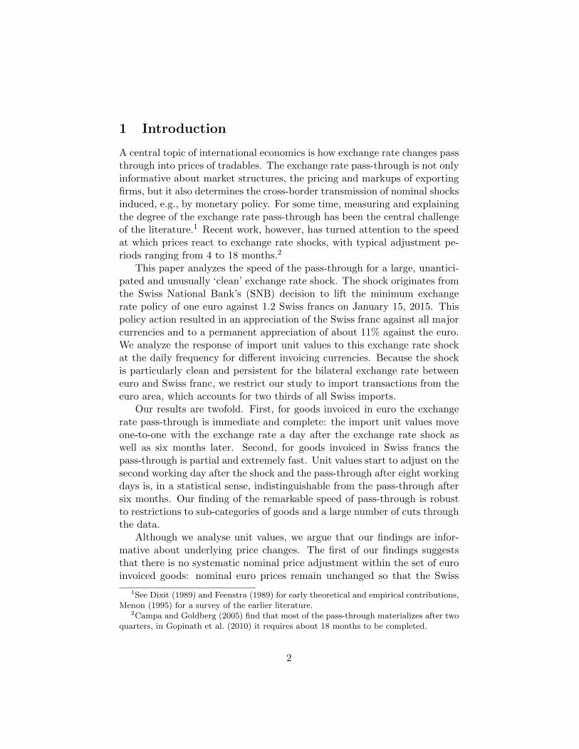
To the best of our knowledge, this paper is the first to estimate the ex-change rate pass-through at the daily frequency. The analysis at the dailyfrequency only makes sense when the underlying shock is sharp and can beunambiguously identified. The large exchange rate shock that originatedfrom the SNB’s policy decision is perfectly suitable in that regard. Figure 1illustrates the dynamics of the nominal bilateral exchange rate (solid line)and the monthly real exchange rate (dots) starting January 1, 2011 throughDecember 31, 2015. On January 15, 2015, the series shows a persistent ap-preciation of about 11% until the beginning of July 2015, at which point theSwiss franc depreciates significantly. Apart from a temporary overshooting,the fluctuations before and after this shock (until July 2015) are mild rela-tive to the drop itself. Further, the forward rates (plus signs) from January14, 2015, which are around the 1.2 threshold, indicate that the exchangerate shock on January 15, 2015 was not anticipated by financial markets.

Figure 1: EURCHF exchange rate from January 2011 to December 2015

11.

11.

21.

3

15 Jan 2011 15 Jan 2012 15 Jan 2013 15 Jan 2014 15 Jan 2015Date

Spot EURCHF exchange rate Real exchange rate (CPI based, Dec 2015 = 1.2)

Forward rates on January 14

EURCHF exchange rate

Sources: SNB, Datastream

The gains from working with an unusually detailed dataset containingthe day and invoicing currency of transactions require us to compromise in

to impact inflation persistence and the determinants of Phillips Curves, as analyzed inBakhshi et al. (2007).

4

other dimensions. The dataset does not allow us to identify exact productsas Gopinath et al. (2010) and thus cannot report the frequency of pricechanges or pass-through rates conditional on price changes. We rely insteadon 8-digit HS product classes similar to Berman et al. (2012). Althoughthis latter study uses firm-level data, we are only able to proxy those witha postal code-product combination.

Our findings contribute to several strands of the pass-through literature.Close to our study is Burstein et al. (2005), who document that importand export prices of tradable goods respond rapidly to large exchange rateshocks, although retail prices of tradable goods adapt to a lesser degree dueto distribution costs and general local components. Our study focuses onunit values at the border, confirming that these unit values react promptlyto a large exchange rate shock. In addition, we make two important ad-vancements. First, we refine the time-grid of the analysis, showing that theunit values appear to react very quickly even at the daily scale. Second, wedisentangle price adjustments by groups of invoicing currencies. This latterdecomposition is important to disentangle mechanical and nominal adjust-ment of border prices. In contrast to Burstein et al. (2005), this distinctionallows us to draw conclusions about nominal rigidities.

Our findings connect more broadly to the literature that addresses thedegree, determinants, and characteristics of the (medium-run) exchange ratepass-through. The average degree of an economy’s exchange rate pass-through into import prices is typically found to vary between 0.4 (a 10%appreciation in the exporter’s exchange rate is associated with a 4% rise inimport prices) and 1 for most countries (see Campa and Goldberg (2005),whose estimate for Switzerland is 0.9) and varies across sectors (e.g., Feen-stra (1989)).5 Our estimates of exchange rate pass-through between 1 (forimports invoiced in euro) and 0.6 (for imports invoiced in Swiss francs) is inline with these previous estimates.

The sharp difference of the exchange rate pass-through across currencygroups documented in our analysis is very much in line with the recent lit-erature, which highlights the role of invoicing currencies for the exchangerate pass-through.6 Specifically, Gopinath et al. (2010) show that the ex-

5A fast growing literature has identified a number of firm- and product-specific de-terminants of the exchange rate pass-through. Recent empirical contributions highlightthe role of firm size, e.g., Berman et al. (2012), the share of imported inputs, e.g., Amitiet al. (2014), or the role of product quality, e.g., Chen and Juvenal (2016) and Auer et al.(2014).

6There is a large literature on optimal invoicing currency, for example, Bacchetta andVan Wincoop (2005), Engel (2006), and Goldberg and Tille (2008). Our study is silent on

5

change rate pass-through into U.S. import prices is complete for non-dollarinvoiced imports, but slow and moderate for U.S. dollar invoiced imports.Gopinath (2015) reinforces this point, writing that “international prices, intheir currency of invoicing, are not very sensitive to exchange rates” andconcludes that “a good proxy for the sensitivity of a country’s traded goodsinflation to exchange rates is the fraction of its imports invoiced in a foreigncurrency.” Our results, in particular those of the euro invoiced sample, showthat these findings also tend to hold for the case of a small open economyand under a large exchange rate shock.

Regarding our more specific focus on the speed of price adjustment, theexisting empirical evidence suggests that in normal times this speed of ad-justment is rather limited. Campa and Goldberg (2005) observe that “[m]ostof the pass-through response occurs over the first and second [quarter] af-ter an exchange rate change” although Gopinath et al. (2010) analyze moredetailed transaction-level import prices and find that the pass-through re-quires about 18 months to be completed. Burstein and Jaimovich (2012), inturn, find quicker adjustments using Canadian and U.S. scanner data. Theyshow that retail prices adjust to exchange rate shocks within about fourmonths. Gorodnichenko and Talavera (2016) show that price adjustment iseven faster in the particular case of online markets. We complement thisrich set of findings by analyzing the speed of exchange rate pass-though intounit values of imported products at the daily frequency. We attribute theexceptionally fast pass-through to the fact that we analyze a particularlylarge exchange rate shock. As stressed in a recent study by Alvarez et al.(2016), profit maximizing firms may optimally chose not to adjust prices tosmall shocks, while the need to adjust prices quickly may rise in the face oflarge shocks (see also Corsetti et al. (2008)).

Our work also connects to the strand of empirical research on episodes oflarge exchange rate changes. Previous studies have examined large exchangerate devaluations mainly for developing countries. Verhoogen (2008) consid-ers the large Mexican devaluation in 1994 as the exchange rate shock. Flach(2016), for example, uses the depreciation of the Brazilian real to identifyits causal effects on export prices. Further, Cravino and Levchenko (2015)use the devaluation of the peso during Mexico’s “Tequila Crisis” and showits distributional effect on income. Alessandria et al. (2015) consider exportexpansion in emerging markets after a large devaluation. Efing et al. (2015)examine the impact of the Swiss franc exchange rate shock from January

this issue, but similar to Gopinath et al. (2010) and Devereux et al. (2015) take insteadthis choice as given.

6

15, 2015 on investor behavior and the real economy on the monthly level.We contribute to this literature on large exchange rate shocks in that weanalyze the pass-through of a single-day, large, and unanticipated exchangerate appreciation. Our large exchange rate shock, moreover, is novel to theliterature in that it concerns an industrialized country and a major currency.

By suggesting fast and immediate price adjustments after a large ex-change rate shock, we connect to the empirical literature on state-dependentpricing. Using Mexican consumer price data, Gagnon (2009) shows that thefrequency of price adjustments comoves with inflation and concludes that“pricing models should endogenize the timing of price changes if they wishto make realistic predictions at both low and high inflation levels.” Ourfindings support this general message.7 Related empirical work addressesinternational price settings using large micro-datasets at ever higher fre-quencies. Auer and Schoenle (2016) and Gopinath et al. (2010) work withsimilar datasets at the monthly frequency. Burstein et al. (2005) and Gorod-nichenko and Talavera (2016) use ‘scanner’ (barcode) data and web-basedretailers at the weekly frequency.

Finally, we claim that our work makes advances by addressing problemsarising due to the endogeneity of exchange rates. It is well known thattraditional pass-through estimations suffer identification problems becauseexchange rates are endogenous.8 Our shock, however, was unanticipatedand ‘purely nominal’. In other words, the shock does not result from funda-mentals so that our estimated price adjustments are not mixing reactions tothe nominal exchange rate and, simultaneously, to shocks to fundamentals.9

7Feltrin and Guimaraes (2015), for example, use prices of Brazilian CPI behavior inBrazil following the large devaluation of the Brazilian real in 1999 and show that thefrequency of adjustment is higher right after the depreciation. Grinberg (2015) uses microdata from Mexican CPI and shows that “the effects of nominal rigidities in retail pricesare quantitatively small and short-lived”, concluding that models with “time-dependentnominal frictions in prices (e.g. Calvo prices) can substantially underestimate the responseof prices to a large depreciation, implying large real effects of the nominal shock”.

8Corsetti et al. (2008) observe that “the estimation bias in pass-through regressionsis a function of the volatility of the nominal exchange rate and the covariance betweenthe exchange rate and the determinants of import prices.” The authors present a modelof variable firm markups and sticky prices where exchange rates and nominal prices aredriven by productivity shocks. With concrete reference to a specific good, Gopinath et al.(2010) write that “the Canadian exchange rate is more likely to be driven by the priceof its main export commodities than the other way round.” Although this criticismis especially prevalent for ‘commodity currencies’ (see Chen and Rogoff (2003)), reversecausality will always affect traditional estimation to some degree. In a related paper,Forbes et al. (2015) show that the the nature of shocks matters for the degree of theexchange rate pass-through.

9In the appendix, we also discuss the possibility that lagged exchange rates bias tradi-

7

The remainder of the paper is organized as follows. Section 2 describesthe nature of the exchange rate shock and the transaction-level trade data.Section 3 first presents the empirical results at the monthly frequency. Thisis done to facilitate comparison with the previous literature, which primarilyprovides estimates at the monthly frequency. The main results at the dailyfrequency are then exposed. Section 4 presents further robustness checks onthe speed of price adjustment. Section 5 concludes.

2 Data description

Our empirical estimates of the speed of exchange rate pass-through relies,first, on a large and exogenous exchange rate shock and, second, on detailedtransaction-level trade data at the daily frequency. The discussion of thesetwo features is divided into two subsections. The next subsection discussesthe SNB’s exchange rate floor and why its lifting has generated an exogenousshock. Thereafter, we discuss the main features of the Swiss customs data.

2.1 The exchange rate shock

This subsection describes the exchange rate shock in detail, arguing thatthe appreciation was exogenous to firms’ border pricing. Moreover, it docu-ments that the exchange rate shock was preceded by an extended period ofexceptional exchange rate stability.

The SNB pursued a policy of a minimum exchange rate of 1.2 Swissfrancs against the euro from September 6, 2011 to January 15, 2015. Thisunconventional policy was introduced in response to the appreciation pres-sures on the Swiss franc during the summer months in 2011. In particular,the Swiss franc had appreciated against the euro by more than 20% in Juneand July 2011. At the time, the SNB argued that the rapid appreciationof the Swiss franc would harm the Swiss economy through imported defla-tion.10 Throughout the period of the minimum exchange rate policy, it wasrepeatedly mentioned that the Swiss franc was overvalued and that the SNBwas fully committed to the policy.

Figure 1 in the introduction plots the nominal EURCHF exchange rate(daily data), the real EURCHF exchange rate (monthly data) and the EUR-

tional pass-through estimates.10The SNB press release from September 6, 2011 stated “[t]he current massive overval-

uation of the Swiss franc poses an acute threat to the Swiss economy and carries the riskof a deflationary development.”

8

CHF forward rates on January 14, 2015.11 During the period of the min-imum exchange rate (September 6, 2011 to January 15, 2015), the Swissfranc fluctuated between 1.2 and 1.25. Yet for most of the floor’s period,the Swiss franc hovered near the minimum rate. The figure also shows thatthe real EURCHF exchange rate (available at monthly frequency) closelytracks the nominal EURCHF over the entire period from January 2011 toJune 2015. The period of exchange rate stability ended abruptly with thelifting of the floor on January 15, 2015. The timing of the SNB’s announce-ment was motivated by the changing global market conditions, in particular,increasing differentials in monetary policy actions.12 We therefore take theEURCHF exchange rate shock as exogeneous to firms’ pricing strategies.

The SNB’s announcement to terminate its policy of the minimum ex-change rate took financial markets by storm.13 Figure 1 shows that theSwiss franc appreciated by 11% against the euro by the end of January.The daily EURCHF rate averaged 1.057 for the post-minimum exchangerate period until June 30, 2015.

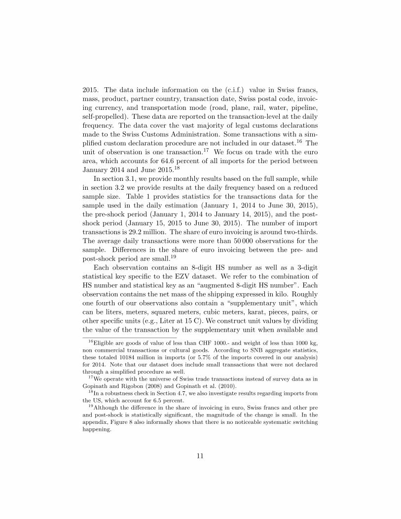
The exchange rate shock was not only large and persistent, but it was alsounanticipated. Figure 2 zooms in on January 2015 and contains informationon EURCHF forward rates. More specifically, it shows that the forwardrates from January 14, 2015, i.e., one day before the SNB’s announcement(diamonds), stayed at the minimum rate of 1.2. Note that the +/- impliedstandard deviations of the forward rates are also included when available.The implied standard deviations of the January 14 forward rates are small,indicating little uncertainty.14 Forward rates quoted on January 16, 2015(triangles), February 13, 2015 (squares) and March 13, 2015 (circles) arealso shown. These forward rates first dropped to about 0.98 the day rightafter the announcement before stabilizing at just under 1.06 in Februaryand March. The implied standard deviation on January 16 is substantially

11The real exchange rate is constructed using the CPI indices from the euro area andSwitzerland and is normalized to 1.2 for December 2014.

12The SNB press release from January 15, 2015 stated “[r]ecently, divergences betweenthe monetary policies of the major currency areas have increased significantly a trend thatis likely to become even more pronounced. ... In these circumstances, the SNB concludedthat enforcing and maintaining the minimum exchange rate for the Swiss franc againstthe euro is no longer justified.”

13The list of market commentary regarding the SNB’s decision on January 15, 2015is long. One of many examples is from Reuters, see http://www.reuters.com/article/us-swiss-snb-cap-idUSKBN0KO0XK20150116.

14For a study looking at whether the announcement was anticipated or not, see Mirkovet al. (2015) who look at various Swiss francs options quotes in a narrow time frame aroundthe announcement of the removal of the floor and conclude that no abnormal behaviorpreceded the removal of the floor.

9

Figure 2: EURCHF spot rates and forward rates with implied standarddeviations from January 2015 to June 2015

.91

1.1

1.2

15 Jan 2015 15 Mar 2015 15 May 2015Date

Spot EURCHF exchange rate Forward rates on January 14

Forward rates on Jan 14 +/- 1 imp. std Forward rates on Jan 16

Forward rates on Jan 16 +/- 1 imp. std Forward rates on February 13

Forward rates on February 13 +/- 1 imp. std Forward rates on March 13

Forward rates on March 13 +/- 1 imp. std

Forward rates and implied volatility

Sources: SNB, Datastream, own calculations.

higher than before the shock, indicating a higher uncertainty, and lessenssubstantially in February, which is consistent with the shock having beenabsorbed by market participants and the new exchange rate equilibria havingbeen reached.

These observations underpin the view that the exchange rate drop wasnot only large but also unanticipated and exogenous to firms’ pricing deci-sions.

2.2 Swiss customs data

The source for the trade data is the Swiss Customs Administration or Ei-dgenossische Zollverwaltung (EZV), which records Swiss customs transac-tions.15 The full available sample is from January 1, 2012 to December 31,

15The geographical coverage is Switzerland, Liechtenstein, and the two enclaves Cam-pione d’Italia and Busingen.

10

2015. The data include information on the (c.i.f.) value in Swiss francs,mass, product, partner country, transaction date, Swiss postal code, invoic-ing currency, and transportation mode (road, plane, rail, water, pipeline,self-propelled). These data are reported on the transaction-level at the dailyfrequency. The data cover the vast majority of legal customs declarationsmade to the Swiss Customs Administration. Some transactions with a sim-plified custom declaration procedure are not included in our dataset.16 Theunit of observation is one transaction.17 We focus on trade with the euroarea, which accounts for 64.6 percent of all imports for the period betweenJanuary 2014 and June 2015.18

In section 3.1, we provide monthly results based on the full sample, whilein section 3.2 we provide results at the daily frequency based on a reducedsample size. Table 1 provides statistics for the transactions data for thesample used in the daily estimation (January 1, 2014 to June 30, 2015),the pre-shock period (January 1, 2014 to January 14, 2015), and the post-shock period (January 15, 2015 to June 30, 2015). The number of importtransactions is 29.2 million. The share of euro invoicing is around two-thirds.The average daily transactions were more than 50 000 observations for thesample. Differences in the share of euro invoicing between the pre- andpost-shock period are small.19

Each observation contains an 8-digit HS number as well as a 3-digitstatistical key specific to the EZV dataset. We refer to the combination ofHS number and statistical key as an “augmented 8-digit HS number”. Eachobservation contains the net mass of the shipping expressed in kilo. Roughlyone fourth of our observations also contain a “supplementary unit”, whichcan be liters, meters, squared meters, cubic meters, karat, pieces, pairs, orother specific units (e.g., Liter at 15 C). We construct unit values by dividingthe value of the transaction by the supplementary unit when available and

16Eligible are goods of value of less than CHF 1000.- and weight of less than 1000 kg,non commercial transactions or cultural goods. According to SNB aggregate statistics,these totaled 10184 million in imports (or 5.7% of the imports covered in our analysis)for 2014. Note that our dataset does include small transactions that were not declaredthrough a simplified procedure as well.

17We operate with the universe of Swiss trade transactions instead of survey data as inGopinath and Rigobon (2008) and Gopinath et al. (2010).

18In a robustness check in Section 4.7, we also investigate results regarding imports fromthe US, which account for 6.5 percent.

19Although the difference in the share of invoicing in euro, Swiss francs and other preand post-shock is statistically significant, the magnitude of the change is small. In theappendix, Figure 8 also informally shows that there is no noticeable systematic switchinghappening.

11

Table 1: Summary statistics

Total sample Pre-shock period Post-shock periodImports (euro area to Switzerland)

Based on transactions

Average unit value (log) 3.469 3.504 3.397(2.218) (2.213) (2.227)

Share invoiced in EUR 0.676 0.668 0.692Share invoiced in CHF 0.315 0.322 0.299Share invoiced in other currencies 0.009 0.009 0.009Share with available supp. units 0.244 0.243 0.248

Based on (log) value

Share invoiced in EUR 0.659 0.654 0.672Share invoiced in CHF 0.322 0.328 0.308Share invoiced in other currencies 0.018 0.017 0.021Share with available supp. units 0.300 0.298 0.307

Number of transactions 29193685 19762630 9431055

Average number of daily transactions 53468.29 52006.92 56813.59(33553.95) (32601.74) (35513.52)

Average EZV EURCHF exchange rate 1.176 1.226 1.057(0.079) (0.009) (0.018)

Note: standard deviations are shown in parantheses. The total sample spans from January1, 2014 to June 30, 2015. The pre-shock period goes from Janury 1, 2014 to Janury 15,2015 while the post-shock period goes from January 16, 2015 to June 30, 2015.

by the mass when not.Our dataset contains two additional variables, which are key for the

empirical exercise.20 The first key variable is the transaction date. Unlikeother trade data, and fortunately for our purpose, the transaction date isnot recorded at the monthly but at the daily frequency. More precisely,the transaction date (Veranlagungsdatum) reports the day when the goodsphysically cross the border. Given the unique identification of our exchangerate shock – January 15, 2015 – the daily frequency of our data is of greatvalue to identify the dynamics of price reactions in the very short run and,in particular, the speed of exchange rate pass-through.

The second key variable records the currency in which transactions areinvoiced. For each customs declaration, we know whether the invoicing cur-rency was either of the following five categories: CHF, EUR, USD, other EU

20The EZV data have been previously used at the monthly level by Kropf and Saure(2014) and Egger and Lassmann (2015).

12

currencies and other non-EU currencies. If the transactions are not invoicedin Swiss francs, the value is converted using a specific exchange rate. Theexchange rate used for imports is published daily by the EZV. It correspondsto the market exchange rate observed the working day before the declara-tion is made. For example, if a transaction is declared on a Monday, theFriday exchange rate is used. The exchange rate is published early in themorning (e.g. 04:30 am for December 14, 2015). On January 15, 2015, inparticular, the exchange rate was published before the SNB’s announcementand its value for January 15, 2015 (applicable to the January 16, 2015 trans-actions) is 1.21303. However, the EZV allowed a non-published exchangerate to be used for transactions registered on January 16 if appropriatejustifying documents were produced by importers.21 Unfortunately, sinceseveral transactions can be declared under a single custom declaration butthe currency of invoicing is reported at the declaration level, it may happenthat transactions invoiced in different currencies are classified under a singlecurrency. In these occurrences, the currency covering the most of the dec-laration’s value is entered, and our dataset attributes this currency for alltransactions. We remedy this shortcoming by a robustness check restrictingthe sample to customs declarations with a single cross-border transaction.

The currency information is important not only because the invoicingcurrency is known to be a crucial determinant of the exchange rate pass-through. More importantly, under sticky prices and by pure mechanics, theexchange rate shock is in the short run (i) fully passed through into importprices in the case when transactions are invoiced in exporter currency and(ii) not passed through at all in the case when transactions are invoicedin importer currency. The distinction between CHF, EUR, and all othercurrencies is therefore crucial to identify the speed of actual pass-throughvia active price adjustments.

Our analysis focuses on transactions invoiced in Swiss francs and eurossince our exercise concentrates on transactions between Switzerland and theeuro area, the vast majority of which is invoiced in either of the two cur-rencies. Figure 3 plots shares of Swiss imports from the euro area invoicedin Swiss francs, euros, or other currencies from January 2014 to December2015 at the monthly frequency. The shares are computed based on transac-

21For exports, the same rule applies in general. However, the monthly average exchangerate or the ‘international groups’ internal accounting exchange rate can be used if thefirm has an according arrangement and is registered with the EZV. The monthly averageapplicable to a transaction in month, m, is the average of the daily exchange rate observedbetween the 25th of the month m− 2 and the 24th of the month m− 1. The uncertaintyas to which exchange rate was used motivates our focus on import transactions.

13

tions (left panel) and based on values (right panel). The figure conveys twomessages. First, almost all trade is invoiced either in Swiss francs or euros.Second, the respective shares are stable over time and, in particular, do notappear to have shifted in response to the exchange rate shock in January2015.

To assess whether firms switch the invoicing currency, Figure 3 also re-ports the share of transactions (value) that stem from the subset of triplets ofHS-product, postal code, and partner country (proxying firms), that have al-ways invoiced in the same currency throughout the 18-month sample. Theseshares are indicated by the dashed lines, which separate the Swiss franc oreuro shares into two areas. The area between the dashed lines consists oftransactions from triplets who always invoiced in the respective currency.These are between a quarter to half of the respective shares.22

Despite the detailed information on date and invoicing currencies, thereare important limitations to the transaction-level data. First, we do notobserve prices of unique goods but are limited to the augmented 8-digitcategories of the HS classification system, which means that our study relieson unit values instead of prices. The limitation implies, in particular, thatwe are unable to directly measure price stickiness. Although unit values aregenerally contaminated by compositional product and quality shifts insidea goods category, we argue below that this is unlikely to drive our results.

A second limitation of our dataset is that intrafirm transactions are notidentified.23 Thus, we cannot exclude them from the analysis to extractonly market price reactions to the exchange rate shock as in Gopinath et al.(2010). We address this shortcoming by analyzing intermediate and invest-ment goods separately from final consumption goods in a robustness checkand by looking at transactions of small values that are unlikely to be subjectto intrafirm trade in robustness checks.

3 Estimation strategy and results

This section presents our main findings. We begin by providing resultsfrom a standard pass-through estimation on the full available data, beforezooming in on a short window to estimate the daily reaction of unit values

22See, Appendix 2 for further information on the extent of switching from one invoicingcurrency to another in response to the exchange rate shock.

23Neiman (2010) shows for U.S. transactions data that prices of intrafirm trade are lesssticky, but that the pass-through is still not immediate.

14

Figure 3: Monthly shares of currency in the Swiss imports from the euroarea

.2.4

.6.8

1

20152014date

Based on transactions

.2.4

.6.8

1

20152014date

Based on values

Other EUR CHF

The dark area represents the share of transactions (value) invoiced in Swiss francs, thelight area in euros and the gray area in other currencies. The area between the dashed linesrepresents the share of transactions (value) originating from triplets (postal code - HS -country) that always invoiced in the same currency from January 2014 to December 2015.The areas outside the dashed lines represent the share of transactions (value) originatingfrom a triplets that have invoiced in different currencies.

to the January 15, 2015 shock.

3.1 Monthly estimations

The total available sample stems from January 2012 to December 2015.Given the high number of transactions this represents, we are unable to runa transaction-level regression on the full time window. To gauge the behav-ior of the pass-through over the full sample, we start by estimating a stan-dard pass-through regression model similar to Gopinath et al. (2010) at themonthly frequency, on a panel of postal code - augmented HS-classification- partner country triplets. At each month, we define pi,t as the median unitvalue of the triplet i and estimate the following model:

15

ln(pi,t) = αi +

M∑m=0

βm ln(et−m) +

M∑m=0

δm ln(CPIi,t−m) +Xi,tγ + εi,t, (1)

where i indicates one triplet (i.e., postal code - augmented HS-classification -partner country) and t a month. In our baseline specification, the dependentvariable, pi,t, is the median unit value of the imported triplet.24 The bilateralexchange rate, et is expressed in CHF per EUR. The EZV exchange rate doesnot carry any index of the parter country because the focus of our analysis ison Swiss trade with the euro area. CPIi is the CPI of the exporter country.Xi,t represents a range of control variables. These include fixed effects ofeach triplet, partner country - 2-digit HS specific trends and 4 quarterlyGDP lags of the importer (Switzerland). Separate regressions are run fortransactions invoiced in euro and in Swiss franc. In all specifications, wecluster standard errors at the postal code level.

Model (1) is specified in levels instead of changes. This choice is mo-tivated by the fact that our data have a strongly unbalanced structure, assome triplets don’t appear every month in the sample. Excluding these ob-servations would result in a sample bias towards triplets that trade regularlyand may be more likely to adjust prices frequently, thus potentially over-estimating the pass-through and resulting in results not comparable to theones presented in the daily section. The 2-digit HS - partner country specifictrend ensures that suitable fixed effects remain when differencing equation(1).25

The exchange rate movement during the full sample comprises the floorperiod, with little exchange rate variation, the January 15, 2015, shock, andthe post-floor exchange rate movements. It is clear from Figure 1 that mostof the exchange rate variation is coming from the shock, and that the resultsof the regression are mostly representing the reaction to the shock.

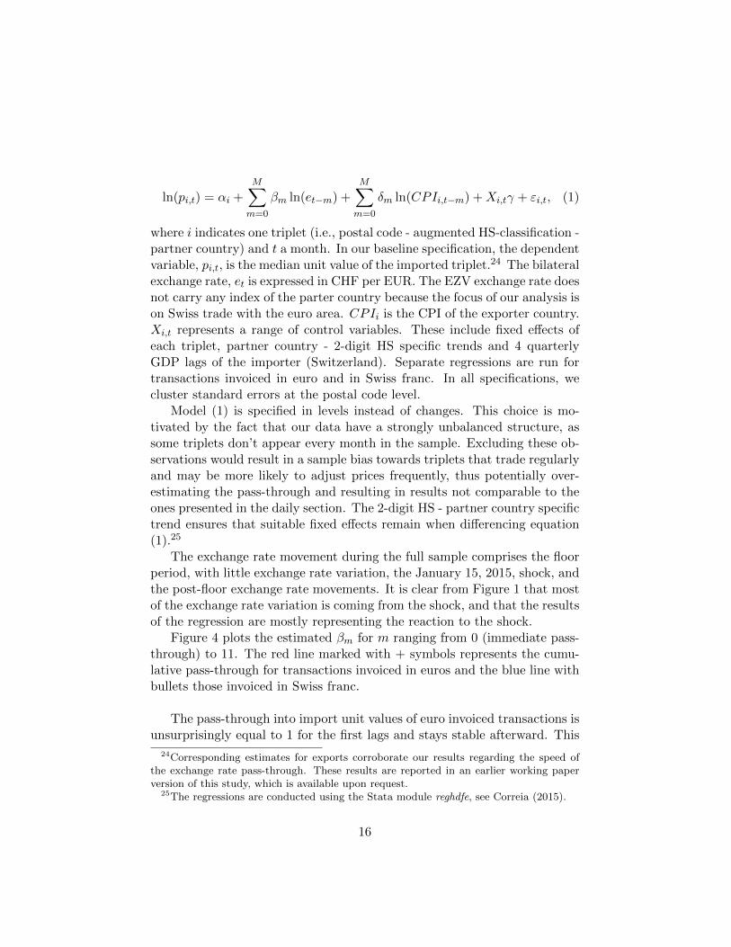
Figure 4 plots the estimated βm for m ranging from 0 (immediate pass-through) to 11. The red line marked with + symbols represents the cumu-lative pass-through for transactions invoiced in euros and the blue line withbullets those invoiced in Swiss franc.

The pass-through into import unit values of euro invoiced transactions isunsurprisingly equal to 1 for the first lags and stays stable afterward. This

24Corresponding estimates for exports corroborate our results regarding the speed ofthe exchange rate pass-through. These results are reported in an earlier working paperversion of this study, which is available upon request.

25The regressions are conducted using the Stata module reghdfe, see Correia (2015).

16

Figure 4: Cumulative pass-through on import unit values

0.2

.4.6

.81

1.2

0 5 10Lag (month)

EUR invoiced CHF invoiced

Based on a monthly triplet panel regression including controls for ex-porter’s CPI and importer’s GDP (specification (1)). Errors are clus-tered at the postal code level. The sample spans January 2012 toDecember 2015.

finding mirrors the result uncovered in Gopinath et al. (2010) of full andstable pass-through for import transactions invoiced in the foreign currency.

For transactions invoiced in Swiss francs, the results are more surprising.The immediate pass-through of around 0.4 indicates that unit values arereacting to the exchange rate movement within the same month. Even morestriking is the fact that the initial pass-through is close to the longer-runcumulative pass-through of 0.65. This indicates that a large proportion ofthe pass-through is attained within the month of the shock rather than witha delay.

3.2 Daily estimation results

Motivated by the remarkably fast pass-through uncovered at the monthlyfrequency, especially for Swiss franc invoiced transactions, we next use dailydata to obtain more precise estimates of the reaction to the shock. The esti-mation of equation (1) provides a measure of the effect of exchange rate onthe unit values based on the whole sample. While most of the exchange rate

17

variation in the sample comes from the January 15, 2015 shock, estimatingequation (1) delivers imprecise results if the reaction to that large shock dif-fers from reactions to small shocks. To ensure that we capture the reactionto the large shock only, we estimate an equation with daily dummies rightbefore and after January 15, 2015. Specifically, we reduce the sample toJanuary 2014 to June 2015 and perform an event-study analysis based onthe following daily specification,

ln(pk) = αikjksk +31∑

d=−8

βDd Ddk +

5∑m=2

βMmMmk +Xkγ + εk. (2)

Here, k is a single transaction, pk is the unit value, ik is the product classifi-cation of transaction k, jk is the partner country, and sk is the postal code.Dd

k is a daily (working day) dummy that equals one if the day of transactionk equals d and zero otherwise. We add daily dummies from the first Mondayof 2015 (January 5th, defined as d = −8 so that January 15th is d = 0 ) tothe last working day of February (February 27th, d = 31). The dummiesbefore January 15 capture a potential anticipation of the shock’s effect onunit value, while the ones after capture the daily evolution of the level ofunit values after the shock. Mm

k are monthly dummies from March 2015 toJune 2015, taking value 1 if the transaction k happens within the month mand 0 otherwise. They capture the monthly level in unit values after theperiod covered by daily dummies. Xk represents the controls including a setof country - HS2 specific time trends. We treat weekend transactions as ifthey take place on Fridays.26

We stress that the model specified in (2) reflects our aim to exploitthe variation of the large exchange rate shock of January 15, 2015 and toestimate the subsequent reaction of unit values on a fine resolution of thetime dimension. Specifically, the use of daily dummies ensures that onlychanges of unit values on a specific day are captured, which can then berelated to the corresponding exchange rate movements. The high frequencyof dummies in equation (2) enables us to interpret the coefficient of thedaily dummies close in time to the shock as capturing the shock’s effect: asargued in section 2.1, the absence of significant exchange rate changes beforethe shock ensures that no lagged exchange rate movement contaminates ourestimation in the days following the shock. Other price determinants such asmarginal costs are also unlikely to change in the few weeks after the shock.

26Weekend transactions represent 3.07% of the number of transactions (Saturday is2.5%, Sunday is 0.57%), and 1.71% of total value (1.49% for Saturday and 0.22% forSunday).

18

The downside of this specification is that it is less readily comparable withstandard specifications that rely on exchange rate lags as the one defined inequation (1).27

Based on the daily estimation, we also provide measures of start andend of the pass-through, which then give rise to the definition of the speedof pass-though (and thus justify the present paper’s title). For transactionsinvoiced in Swiss francs, the start of the adjustment is defined as the firstday for which the cumulative change in unit values (the estimated βDd in(2)) is different from the pre-shock daily dummies average. The end of theadjustment is defined as the first day for which the daily dummy is differentfrom the pre-shock average and the ratio between the cumulative change inunit value and the cumulative change in the exchange rate is not significantlydifferent from the medium-run pass-through ratio, which is defined as theaverage of the four monthly pass-through ratios. When the medium-runpass-through is not different from 0 in the Swiss franc, we define no start norend of adjustment.28 Because of the weak response in unit values expressedin euros, we do not define start nor end day of adjustment for transactionsinvoiced in euros.

For expositional purposes, our estimates corresponding to daily transac-tions are presented in graphical form. They include plots of the daily co-efficients for euro and Swiss franc invoiced transactions together with their95% confidence intervals. The medium-run (monthly) estimates are also in-cluded in the same plots. Their coefficients are denoted as circles with 95%

27We cannot exclude the possibility that exchange rate movements after the shock areinfluencing unit values in periods further away from the shock, so that the value of monthlydummies for March to June only give an imprecise estimate of the effect of the January 15shock. One substantial shock to the EURCHF exchange rate occurs in July 2015, which isexcluded from our sample. The standard models, however, produce estimated coefficientsthat rely on the exchange rate variation of the whole period, which is not the aim of ourstudy.

28Formally, we first define the pre-shock level as the average of the coefficient on dum-mies D−8 to D0 (PRE = 1

9

∑0i=−8 β

Di ), and, for each daily or monthly dummy, we define

a “pass-through” ratio PTd =βDd −PREEd

, where Ed is the cumulative change in the ex-

change rate from January 15th to day or month d. dstart is such that the null hypothesisPTdstart = 0 is rejected and PTi = 0 is not rejected for all 0 < i < dstart. dend is suchthat the null hypothesis PTdend = 1

4

∑m PTm where m covers all months after the daily

dummies, namely March to June 2015, is not rejected, although PTdend = 0 is rejected.A shortcoming of this approach is that the wider the standard errors of our estimates are,the easiest it is to not reject equality with the medium-run. To attenuate this, we requirethe end day pass-through not to be significantly different from the medium-run at the10% level instead of the usual 5% level.

19

confidence intervals.29 Vertical dashed and dotted lines indicate the startand end day of adjustment when relevant. The cumulative change in theexchange rate relative to the January 15th pre-shock level is also shown ina blue dashed line.

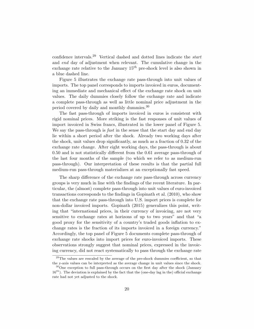
Figure 5 illustrates the exchange rate pass-through into unit values ofimports. The top panel corresponds to imports invoiced in euros, document-ing an immediate and mechanical effect of the exchange rate shock on unitvalues. The daily dummies closely follow the exchange rate and indicatea complete pass-through as well as little nominal price adjustment in theperiod covered by daily and monthly dummies.30

The fast pass-through of imports invoiced in euros is consistent withrigid nominal prices. More striking is the fast responses of unit values ofimport invoiced in Swiss francs, illustrated in the lower panel of Figure 5.We say the pass-through is fast in the sense that the start day and end daylie within a short period after the shock. Already two working days afterthe shock, unit values drop significantly, as much as a fraction of 0.32 of theexchange rate change. After eight working days, the pass-through is about0.50 and is not statistically different from the 0.61 average pass-through ofthe last four months of the sample (to which we refer to as medium-runpass-through). Our interpretation of these results is that the partial fullmedium-run pass-through materializes at an exceptionally fast speed.

The sharp difference of the exchange rate pass-through across currencygroups is very much in line with the findings of the recent literature. In par-ticular, the (almost) complete pass-through into unit values of euro-invoicedtransactions corresponds to the findings in Gopinath et al. (2010), who showthat the exchange rate pass-through into U.S. import prices is complete fornon-dollar invoiced imports. Gopinath (2015) generalizes this point, writ-ing that “international prices, in their currency of invoicing, are not verysensitive to exchange rates at horizons of up to two years” and that “agood proxy for the sensitivity of a country’s traded goods inflation to ex-change rates is the fraction of its imports invoiced in a foreign currency.”Accordingly, the top panel of Figure 5 documents complete pass-through ofexchange rate shocks into import prices for euro-invoiced imports. Theseobservations strongly suggest that nominal prices, expressed in the invoic-ing currency, did not react systematically to pass through the exchange rate

29The values are rescaled by the average of the pre-shock dummies coefficient, so thatthe y-axis values can be interpreted as the average change in unit values since the shock.

30One exception to full pass-through occurs on the first day after the shock (January16th). The deviation is explained by the fact that the (one-day lag in the) official exchangerate had not yet adjusted to the shock.

20

Figure 5: Daily reaction of import unit values

-.2

-.15

-.1

-.05

0.0

5lo

g ch

ange

16 Jan 2015 31 Jan 2015 14 Feb 2015 28 Feb 2015date

EUR invoiced

Start of adj.Jan 19

End of adj.Jan 27

-.2

-.15

-.1

-.05

0.0

5lo

g ch

ange

16 Jan 2015 31 Jan 2015 14 Feb 2015 28 Feb 2015date

CHF invoiced

daily dummies eurchf log-diff. with Jan15 following months

Daily dummies for import unit values (specification 2). The regression includes augmentedHS-postal code-country triplets fixed-effects and a 2-digit HS-country specific trend. Er-rors are clustered at the postal code level. The sample spans January 1, 2014 to June 30,2015.

21

shock into border prices.

Quite on the contrary, the bottom panel of Figure 5 shows a non-negligible short-run pass-through of the exchange rate shock for transactionsinvoiced in Swiss francs. We interpret this key finding as evidence that nom-inal prices did adjust fast and systematically to pass through the exchangerate shock into border prices.31 We acknowledge that we need to argue verycarefully when inferring (unobserved) price changes from the pass-throughinto unit values. In particular, three important factors complicate our in-terpretation of changes in unit values as price changes, potentially inducingchanges in unit values and creating estimation biases. These factors arequality shifts within product classifications, exit from and entry to foreignmarkets by firms or products and, to some extent, firm heterogeneity.

Quality shifts within product categories constitute a fundamental prob-lem when inferring price changes from unit values. We argue, however, thatthey are unlikely to drive the drop in unit values shown in the bottom panelof Figure 5. We corroborate this view by looking at the sign of potentialbiases that would result from a quality shift. We first observe that, follow-ing the exchange rate shock, Swiss consumers can be expected to substitutetowards higher quality in the basket of imported foreign goods, which nowbecome cheaper. Such an effect, however, would increase import unit values,although the average unit value did actually decrease (see Figure 5). Anysubstitution effect should thus attenuate the estimated drop of unit valuesof Swiss imports.32 Finally, we point out that the unit values of importsinvoiced in euros (top panel of Figure 5) remained very stable. Again, thisobservation indicates that strong substitution effects are not affecting thisset of transactions.

Exit and entry of firms or products in foreign markets is a second sourceof potential bias of pass-through estimations. Gagnon et al. (2014) arguethat exit into and entry from export markets may induce an attenuationbias in the pass-through estimations. In the presence of such an attenuationbias, however, the true pass-through would be even larger than our estimatedchanges in unit values for Swiss franc-invoiced goods. Gagnon et al. (2014)

31We do not take a stance on why nominal prices of Swiss franc-invoiced transactionsdid adjust, although those of euro-invoiced transactions did not.

32Also, a similar bias should affect estimates of pass-through into export unit values inthe opposite way: foreigners, for whom prices of Swiss products become more expensive,should substitute towards lower quality, which would generate a drop in unit values afterthe exchange rate shock. If that effect were strong, the estimated drop of unit valuesshould be stronger for exports than for imports. This is not the case, as estimations ofexport unit values (reported in an earlier version of this paper) indicate.

22

also report that empirically the “biases are modest over typical forecasthorizons” and even less so for our short period of two weeks.

Nevertheless, we try to address potential biases due to exit and entry. Wegauge the exit and entry rate around the date of the exchange rate shockby looking at entry and exit of pairs of product and partner country.33

Specifically, for each week, w, we compute the number of those product-country pairs with positive imports within the two weeks, w and w + 1.34

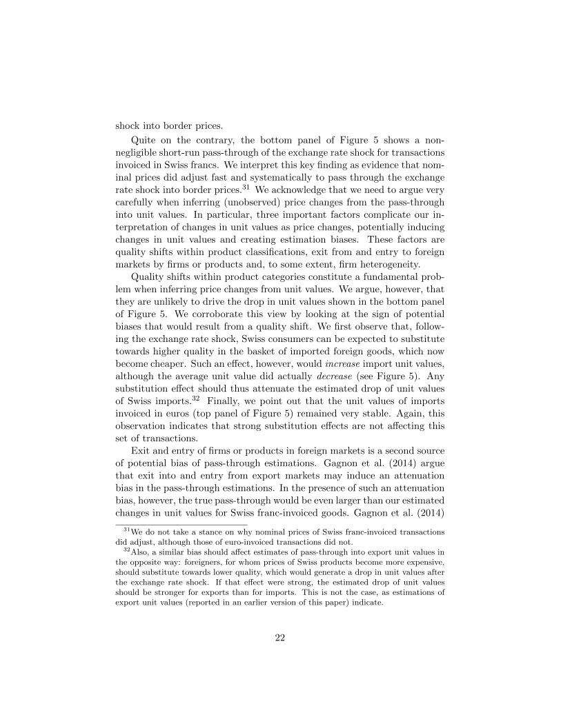
Out of these sets of product-country pairs, we compute the share with zeroimports in the calendar year before w. This share of entrants is plotted inthe top panel of Figure 6 (fat solid line). Also, a corresponding thin dashedline is added as reference for the same period of the preceding year. Weobserve that the figure does not reveal unusual entry dynamics around thedate of the shock (indicated by the vertical line) in terms of levels or relativeto the previous year.

Similarly, for each week w we look at the number of those pairs withpositive imports within the calendar year preceding w. Out of these pairs,we compute the share with zero imports in the two weeks, w and w+1. Thisshare of temporary exiting pairs is plotted in the bottom panel of Figure 6(fat solid line). A corresponding thin dashed line is added as reference forthe preceding year. Again, the figure does not indicate unusual exits aroundthe date of the shock.

Clearly, we cannot observe all exits and entries of firms or products. Yet,the set of exits and entrants that can be identified (those plotted in Figure6) do not indicate that unusual entrance or exit happen in the period afterthe shock within which the adjustment takes place.

Having discussed the potential effects of the two most relevant biases ofexchange rate pass-through into unit values, we conclude that a large partof the sharp and sudden fall in unit values in the immediate aftermath of theexchange rate shock must have been driven by underlying price changes. Ofcourse, this does not imply that price adjustments were identical in magni-tude for all firms or products. Indeed, it is well known that there is hetero-geneous pass-through across firms. For example, Berman et al. (2012) showthat highly productive firms display relatively low import price exchangerate pass-through while Amiti et al. (2014) show that import-intensive ex-porters display relatively low export price pass-through. Clearly, some firms

33We recognize that, by looking at exits and entries of these pairs, we cannot observeall product exits and entries but a subset of them. Indeed, any exiting (entry) of a pairmust reflect at least one product exit (entry) from the market in question, although thereverse is not true.

34The time span of two weeks reflects the period, in which the unit values react.

23

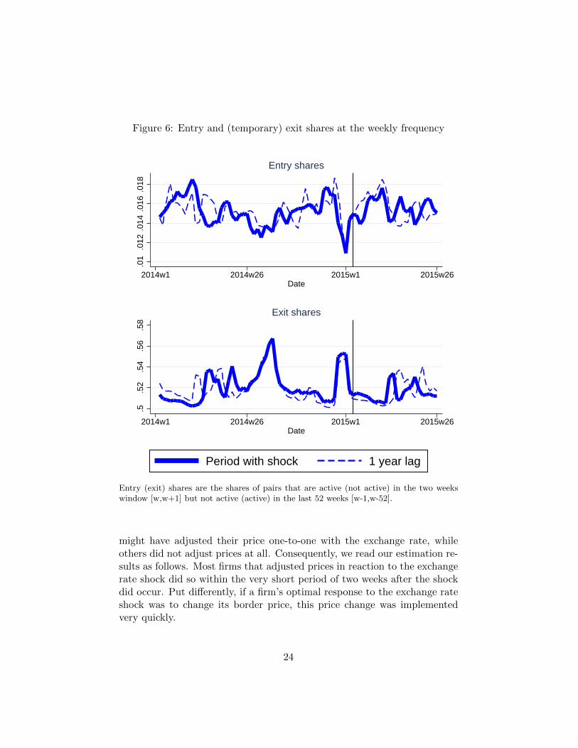
Figure 6: Entry and (temporary) exit shares at the weekly frequency.0

1.0

12.0

14.0

16.0

18

2014w1 2014w26 2015w1 2015w26Date

Entry shares

.5.5

2.5

4.5

6.5

8

2014w1 2014w26 2015w1 2015w26Date

Exit shares

Period with shock 1 year lag

Entry (exit) shares are the shares of pairs that are active (not active) in the two weekswindow [w,w+1] but not active (active) in the last 52 weeks [w-1,w-52].

might have adjusted their price one-to-one with the exchange rate, whileothers did not adjust prices at all. Consequently, we read our estimation re-sults as follows. Most firms that adjusted prices in reaction to the exchangerate shock did so within the very short period of two weeks after the shockdid occur. Put differently, if a firm’s optimal response to the exchange rateshock was to change its border price, this price change was implementedvery quickly.

24

These observations suggest that the fast exchange rate pass-though forgoods invoiced in Swiss francs is driven by underlying nominal price changes.In particular, we read this findings as strong evidence of a prompt price ad-justment in response to a large shock to the Swiss franc on January 15,2015.35 We claim that the price adjustment is clustered in that an uncom-monly high share of firms adjust their prices. The systematic adjustmentstake place within the first two weeks after the shock. Presuming conser-vatively that prices either remain unadjusted or adjust one-to-one with ex-change rates, then about 50% of all import prices invoiced in Swiss francsmust have been adjusted after eight working days (see Table 2). In themedium-run (months 4 to 6) the according pass-through is 0.61. This meansthat under the same assumptions 82% of those prices that were adjusted inthe medium-run were adjusted immediately (0.50/0.61 = 0.82).

Our claim that the share of price adjustments in the sample of Swissfrancs invoiced products increased after the January 15 shock is corroboratedby directly observed price data. Figure 7 plots the year-on-year change ofshares of price changes within the sample of import prices surveyed by theFederal Statistical Office to construct the Swiss import price index.36 Theseprice data are surveyed within the first eight days of each month and arereported at the monthly frequency, so that January 2015 data refer to theperiod before the shock. The top panel corresponds to the sample invoicedin Swiss francs and reveals a sharp increase in the frequency of price changesin February 2015 with a slight lull in March 2015 followed by an increase inthe frequency in April 2015. Thereafter, the pattern of price changes returnsto its pre shock level.37 We attribute the staggered increase in the reportedfrequency of price changes to the fact that the Federal Statistical Officeconducts its monthly survey on a changing sample of products. Therefore,some prices that were changed immediately after the exchange rate shockon January 15 were not surveyed before March or April. The correspondingprice changes therefore appear in the statistics with a delay. The bottompanel plots the corresponding shares of price changes for the sample of goods

35We also acknowledge that we are unable to directly measure price stickiness, asGopinath and Rigobon (2008), who track the frequency of price adjustments. We thuscannot follow Gopinath et al. (2010), who estimate the exchange rate pass-through con-ditional on price adjustments.

36We take year-on-year changes because the sample of prices is specific to each monthof the year. Note that the sample includes goods from all partners and not just from theeuro area.

37The average price change for import prices invoiced in Swiss francs (foreign currency)was 21.7% (10.0%) in the period from 2011 to 2014 and averaged 28.2% (10.3%) for thefirst six months in 2015.

25

invoiced in foreign currency.38 In line with our earlier finding, the increasein the share of price changes is much more moderate for the sample of goodsinvoiced in foreign currencies. We acknowledge that the data underlyingFigure 7 are only partially comparable to those used in our full analysis.Nevertheless, we read the above observations as qualitatively supportingevidence of our preferred interpretation of our central analytical findings.

Our interpretation of fast price adjustments, in turn, implies that nom-inal rigidities play a minor role for the period immediately following theexchange rate shock. The findings reported above thus constitute strongevidence in favor of state-dependent pricing frameworks a la Dotsey et al.(1999) and Golosov and Lucas (2007). We also observe that our findings arehard to explain by pricing models based on sticky information a la Mankiwand Reis (2002). In particular, an economy in which a constant fraction ofagents updates information and pricing plans within each period does notsimultaneously match the frequency of price adjustments in normal timesand the large fraction of price adjustments immediately following the unan-ticipated exchange rate shock. Our work thus highlights that exceptionalprice responses to shocks that are particularly visible or hard to ignore arenot captured by sticky information models. Our findings thus complementAlvarez et al. (2016), who show that the exchange rate pass-through materi-alizes faster in response to large exchange rate shocks than to small shocks.Also, we connect to Nakamura and Steinsson (2008), who provide evidencein favor of menu costs by emphasizing the importance of idiosyncratic shocksas a driving force of price changes.

Finally, we also notice that our findings differ somewhat from those inearlier work by Gopinath and Rigobon (2008) who document that priceadjustments of U.S. import prices in episodes of large exchange rate de-valuations were qualitatively “as expected, but [...] surprisingly weak.”39

Part of this mild reaction may be explained by the fact that the exchangerate devaluations were anticipated, so that some prices were adjusted in ad-vance of the devaluation, which dampened the reaction on impact (see theaccording Figure II in Gopinath and Rigobon (2008)). Moreover, most de-valuation episodes concern developing countries for which trade is typicallyinvoiced in U.S. dollars and thus display low pass-through rates even in the

38Specifically, this sample also includes goods invoiced in USD and other foreign cur-rencies and covers all partner countries.

39The frequency of monthly import price increases (decreases) is shown to fall (rise)by about 5 percentage points, although the average unconditional price change drops byabout -0.5% in the month after the exchange rate devaluation.

26

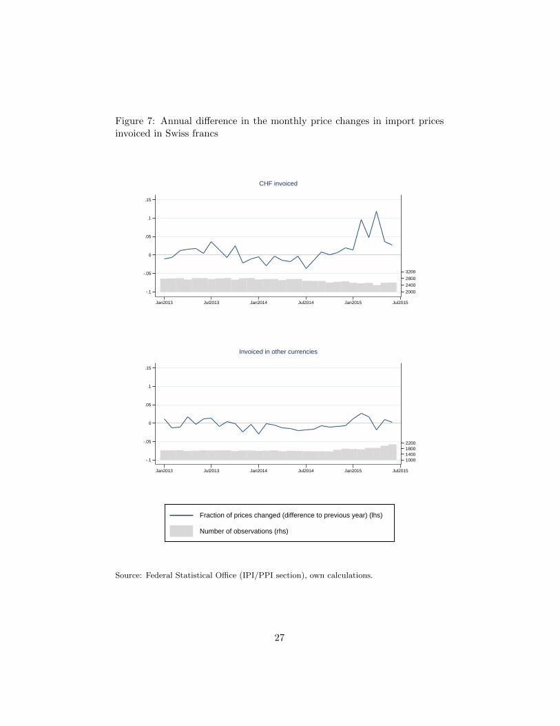
Figure 7: Annual difference in the monthly price changes in import pricesinvoiced in Swiss francs

2000

2400

2800

3200

-.1

-.05

0

.05

.1

.15

Jan2013 Jul2013 Jan2014 Jul2014 Jan2015 Jul2015

CHF invoiced

1000140018002200

-.1

-.05

0

.05

.1

.15

Jan2013 Jul2013 Jan2014 Jul2014 Jan2015 Jul2015

Invoiced in other currencies

Fraction of prices changed (difference to previous year) (lhs)

Number of observations (rhs)

Source: Federal Statistical Office (IPI/PPI section), own calculations.

27

long run (see Gopinath et al. (2010)).40 Thus, the fact that our work un-covers strong reactions by comparison may be traced back to the unusuallyclean and unanticipated exchange rate shock on January 15, 2015, as wellas the substantial differences in invoicing practices between the U.S. andSwitzerland.

Overall, our results suggest a fast adjustment process of nominal prices.Therefore, nominal rigidities seem to have little importance in the face ofsuch a big shock, as import unit values show a fast and persistent pass-through.

A question that remains open so far is how the fast adjustment of borderprices came about in practice. After all, contracts and physical delivery ofcross-border transactions are typically understood to have substantial time-lags, very often exceeding the two weeks of inferred price adjustments.41

In an attempt to address this question, we turn to informal informationobtained through interviews conducted by delegates of the SNB regionalnetwork.42 The interviews revealed that Swiss managers did take uncon-ventional measures to adjust to the appreciation of the franc. Establishedcontracts between Swiss importers and international distributors were im-mediately renegotiated after the shock to maintain the client base. In severalcases, prices were reset automatically, as some contracts contain a built-inclause according to which prices are reset whenever exchange rate changesexceed certain thresholds. The motive behind this practice is to share theimpact of exchange rate changes between parties.43

40Figure II in Gopinath and Rigobon (2008) suggests a cumulative average importprice drop around large devaluations of about 2%, which, given an original shock of 15%,amounts to a pass-through rate of 0.13. This is in the realm of the 24-months pass-throughrate of 0.17 reported for dollar invoiced transactions in Gopinath et al. (2010).

41See Amiti and Weinstein (2011).42The SNB delegates conduct quarterly interviews with about 230 managers and en-

trepreneurs on the current and future economic situation of their companies and on theSwiss economy in general. The selection of companies differs from one quarter to the next.It reflects the industrial structure of the Swiss economy, based on the composition of GDP.The survey’s main results are reported in the SNB’s Quarterly Bulletin. See SNB (2015)for example.

43For exporters, the mirror image emerged. Based on the experiences of the Swiss francshock in 2011, there was the general recognition that an immediate price reduction ofSwiss exports was needed. Some exporting companies whose bargaining position was tooweak (e.g., because of strong competition) absorbed the total cost of the price reductionto defend market-shares. In some cases, prices were even renegotiated for goods that werepurchased before the shock but whose delivery was still outstanding because of deliverylags. Again, this adjustment was done to maintain the client base. The informal infor-mation thus complements and reinforces our main message in suggesting that reactions to

28

4 Robustness checks

This section presents a series of robustness checks on the previous section’smain finding that the speed of price adjustment to a large exchange rateshock is remarkably fast. The robustness checks show that our speed resultholds for numerous subsamples of the dataset. The pass-through for goodsinvoiced in Swiss francs is always fast: in all robustness checks it reaches themedium-run pass-through within 14 working days at most. The most impor-tant restrictions aim to address concerns related to our data limitations butalso to the potential critique of the role of firm-specific and product-specificdeterminants of exchange rate pass-through. These robustness checks arebased on specification (2) and are summarized in Table 2. The correspond-ing graphs of the daily price dynamics are relegated to Appendix 3.

Because our main attention concerns the start and the end day of theexchange rate pass-through, and given that these dates can only be sensiblydefined for transactions that are invoiced in Swiss francs, the results pre-sented in Table 2 are limited to this subset of observations. In other words,we investigate the robustness of our results presented in the bottom panelof Figure 5.

4.1 Unit values versus unit prices

A common critique of analyses based on unit values is that these measuresconstitute not only an imprecise but a potentially biased proxy of actualprices. To address related concerns, we restrict the sample to those prod-ucts and observations for which information on ‘supplementary units’ areavailable. These units represent the economically relevant accounting mea-sure for the goods. Typical units are “pairs” (e.g., for shoes), “pieces” (e.g.,for watches).44 The resulting measures, which we label unit prices, are againimperfect but constitute arguably better measures of prices.

The start and end date for unit prices are listed under the section “Sup.units” in Table 2. Compared to the baseline regression, the estimationsbased on unit prices reveal a comparable speed of the pass-through. Specif-ically, the differences range within the time-frame of two weeks, which con-firms the view that price adjustments are fast. For example, row 1.a in theupper panel of Table 2 presents the results for Swiss franc-invoiced imports

the exchange rate shock were unusually fast.44For example, while declarations for some motor parts only have information on the

mass instead of the number of parts, declarations for watches have the more precise infor-mation of the number of units.

29

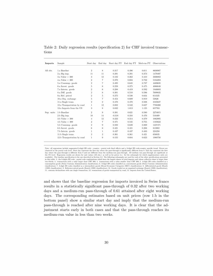
Table 2: Daily regression results (specification 2) for CHF invoiced transac-tions

Imports Sample Start day End day Start day PT End day PT Med-run PT Observations

All obs. 1.a Baseline 2 8 0.317 0.496 0.611 8608987

2.a Big imp. 11 11 0.291 0.291 0.373 1479497

3.a Value > 300 3 12 0.182 0.262 0.410 3306882

4.a Value < 300 2 7 0.370 0.604 0.722 5164283

5.a Consump. goods 2 7 0.495 0.645 0.737 4489635

6.a Invest. goods 5 8 0.259 0.375 0.475 4086848

7.a Interm. goods 2 6 0.288 0.419 0.592 1846683

8.a Diff. goods 2 8 0.301 0.510 0.596 7699835

9.a Ref. priced 2 5 0.275 0.530 0.634 614535

10.a Org. exchange 5 7 0.454 0.609 0.919 53826

11.a Single trans. 2 2 0.470 0.470 0.508 2165627

12.a Transportation by road 1 12 0.082 0.532 0.627 7788390

13.a Imports from the US 3 8 0.832 1.013 1.125 657763

Sup. units 1.b Baseline 2 9 0.381 0.621 0.580 2274015

2.b Big imp. 10 14 -0.318 0.334 0.476 516469

3.b Value > 300 4 12 0.222 0.314 0.379 1062995

4.b Value < 300 2 7 0.471 0.545 0.755 1165622

5.b Consump. goods 2 9 0.592 0.639 0.809 1437471

6.b Invest. goods 6 6 0.421 0.421 0.208 813982

7.b Interm. goods 1 1 0.437 0.437 0.483 224350

11.b Single trans. 2 2 0.361 0.361 0.421 656835

12.b Transportation by road 1 9 0.155 0.684 0.623 1980756

Note: all regressions include augmented 8-digit HS code - country - postal code fixed effects and a 2-digit HS code-country specific trend. Errors areclustered at the postal code level. Start day represent the first day where the pass-through is significantly different from 0. End day represent the firstday where the pass-through is different from 0 and not different from the medium-run pass-through. All medium run pass-through are significant atthe 5% level. Regression results are shown for unit values (All obs.) as well as for prices (i.e. for the subsample for which supplementary units areavailable). The baseline specification is the one described in Section 3.2. The following subsamples are used for each of the other specifications presentedin this table: 2. the 8-digits HS code - postal code combinations which have the largest shares of total imports and whose collective share is larger thantwo-thirds; 3. transactions with a value larger than CHF 300; 4. transactions with a value smaller than CHF 300; 5. 8-digit HS codes classified as aconsumption goods (Swiss Customs Administration classifcation); 6. 8-digit HS codes classified as a investment goods (Swiss Customs Administrationclassifcation); 7. 8-digit HS codes classified as a intermediate goods (Broad Economic Categories (BEC) classification); 8. differentiated goods (Rauch(1999) classification); 9. Reference priced goods (Rauch (1999) classification); 10. Goods traded on an organised exchange (Rauch (1999) classification);11. customs declarations with one single transaction; 12. transactions of goods transported by road; 13. imports from the United-States.

and shows that the baseline regression for imports invoiced in Swiss francsresults in a statistically significant pass-through of 0.32 after two workingdays and a medium-run pass-through of 0.61 attained after eight workingdays. The corresponding estimates based on unit prices (row 1.b in thebottom panel) show a similar start day and imply that the medium-runpass-through is reached after nine working days. It is clear that the ad-justment starts early in both cases and that the pass-through reaches itsmedium-run value in less than two weeks.

30

4.2 Proxying firm size

Our second set of robustness checks aims at addressing the impact of firmsize on our estimations. Berman et al. (2012) show that highly productivefirms absorb more of the exchange rate shocks through export prices andthus exhibit a lower pass-through into import prices. Consistently, Amitiet al. (2014) show that import prices of large, import intensive firms exhibita lower exchange rate pass-through as part of their production costs varywith foreign inputs.45 Equivalently, the speed of response to the shock maydiffer by firm size and import intensity.

While we cannot control for firm characteristics, we nevertheless try toexclude a large share of small importers. Specifically, we restrict the sampleof import transactions to pairs of 8-digit HS code and ZIP-code with thelargest import value. This criterion constitutes only a rough proxy for firmsize, but it does exclude many small Swiss importers. The results are givenin rows 2.a and 2.b in Table 2 and show that the speed of adjustment of 11working days is fast for big importers, too.46

A second and additional way to proxy for firm size is by separatingtransactions of large value from transactions of low value.47 We adopt thevalue of CHF 300 as a threshold to define roughly similarly sized subsamplesof small value shipments and of large value shipments.48 Restrictions 3 and4 in Table 2 show that the medium-run pass-through into import unit valuesis lower for big shipments and higher for small ones. The estimations alsoshow that, again, no notable differences are observed for the start and enddates.

4.3 Intermediate, investment and consumption goods

One of the limitations of our data is that intrafirm transactions are uniden-tified. This drawback may be of importance for the rate of pass-through.For the United States, Neiman (2010) documents that prices of intrafirmcross-border trade display less stickiness. However, the shape of the cu-mulative pass-through reported in Neiman (2010) displays a similar lack

45See also Chung (2016) on the currency choice of import-intensive firms.46In Appendix 3, Figure 10 shows the daily results for imports of big importers.47Kropf and Saure (2014) show that large and productive exporters tend to make ship-

ments of higher values.48Swiss Custom Administration adds a value added tax on imports worth more than

CHF 300. Our results are not sensitive to this threshold. In Appendix 3, Figure 11 showsthe daily results for the import unit values of transactions of less than CHF 300. Figure12 shows the daily results for the import unit values of transactions of more than CHF300.

31

of immediate adjustment for both intrafirm and arm’s length transactions.Nevertheless, it might still be suspected that our fast adjustment resultsfrom multinational firms quickly adjusting their transfer prices.49 Concernsrelated to intrafirm trade are partially addressed by our robustness checksabove, where we have shown that small transactions (those that presumablycorrespond to small and medium sizes firms or to individuals) do not reveala substantially different speed of exchange rate pass-through.

In addition to the robustness checks above, we also address concernsabout intrafirm trade by looking at different goods categories: consump-tion goods, investment goods and raw materials, and intermediate goods.50

Restrictions 5, 6, and 7 in Table 2 show the start and end days with thepass-through estimates for consumption (restriction 5), investment goodsand raw materials (restriction 6), and intermediate goods (restriction 7).51

Some heterogeneity in the medium-run level of pass-through is uncovered,but again, the results show that the adjustment starts rapidly and reachesits medium-run pass-through estimate within nine working days after theshock.

Assuming that the share of intrafirm trade is different across the maincategories, this indicates that intrafirm transactions do not drive our fastpass-through result.

4.4 Differentiated, referenced, and homogeneous goods

With respect to price adjustment, the organization of the market plays asignificant role. Using Rauch (1999) classification, Gopinath and Rigobon(2008) report that the median import price duration is substantially longerfor differentiated goods (14.2 months) than for reference goods (3.3 months)and goods in the organized exchange category (1.2 months). To check thatthe fast pass-through is not driven by the organized exchange or the referencegoods, we run the daily regression on each category separately.52 The results,

49Even in that case, however, the fast adjustment implied by our results would indicatea faster reaction of multinational firms than usual.

50The Swiss customs office classifies each 8-digit HS code as either consumption good,raw material, investment good, energy good, or cultural good. We perform our analysison consumption and raw material and investment goods separately, keeping only thosetransactions whose HS code is classified in a unique category. We use the Broad EconomicCategories (BEC) classification to identify intermediate goods.

51In Appendix 3, Figure 14 shows the daily estimates on import unit values for theinvestment goods and raw material, Figure 13 presents those for consumption goods andFigure 15 those for intermediate goods.

52Due to a lack of sufficient observations, we only regress unit values and are unable tofurther reduce the sample to transactions where unit prices are available.

32

presented in rows 8.a to 10.a in Table 2, show that the level of pass-throughdiffers for each category. Consistent with intuition, goods traded on anorganized exchange show a higher medium-run pass-through, followed byreference priced goods and differentiated goods. Still, the reaction is fast inall three categories. Even differentiated goods show a reaction in unit valuesthe second working day after the shock and reach their medium-term levelafter eight working days.53

4.5 Precision of currency recording

In our description of the Swiss customs data, we have pointed at the possi-bility that the invoicing currency may be misreported for some transactions.Specifically, each customs declaration has a unique invoicing currency butmay contain multiple transactions. In such cases, the invoicing currencyof the main transactions is recorded. This practice may induce biased es-timates, as transactions that are recorded as invoiced in Swiss francs mayactually be invoiced in euros. Consequently, the reaction of unit values oftransactions invoiced in Swiss francs may be overestimated (and similarlythe reaction of unit values of transactions invoiced in euros underestimated).The fact that the euro-invoiced transactions follow the exchange rate changealmost perfectly in Figure 5 already indicates that the misclassification doesnot severely affect our results for euro-invoiced transactions. To formallycontrol for a potential bias, we run the same regressions although restrictingthe sample to transactions for which a misclassified invoicing currency canbe excluded. We do so by focusing on customs declaration with a singletransaction only. The results are listed as restrictions 11.a and 11.b in Ta-ble 2. Consistent with some currency misclassification, they show a lowerpass-through than the full sample. They show however that the speed ofadjustment is fast even in those cases where currency misclassification is im-possible, as the medium-run pass-through is reached after only a few daysin both cases.54

4.6 Product category regressions

We also investigate whether the speed of price adjustment differs acrossHS categories by running separate regressions for each HS section. Table 3

53In Appendix 3, Figure 16 shows the daily estimates on unit values. It is notable thatthe exclusion of the more volatile organized exchange and reference categories lead to moreprecise estimates of the daily reaction.

54In Appendix 3, Figure 17 show the daily results for transactions where currencymisclassification is not possible for imports.

33

presents the section specific results, which show substantial heterogeneity inthe medium-run pass-through, with some categories showing no significantmedium-run pass-through and other displaying full-pass-through.

Whenever the pass-through is nontrivial, however, the medium-run pass-through is reached within a short time window.55

Table 3: Imports daily regression results (CHF invoiced, by HS section)

Start day End day Start day PT End day PT Med-run PT Observations

Live animal; animal pro~s 4 4 0.592 0.592 0.686 35222

Vegetable products 2 2 0.326 0.326 0.488 300601

Animal or vegetable fat~l 7 7 0.707 0.707 0.895 9544

Prepared foodstuff; bev~s 2 3 0.337 0.632 0.690 769461

Mineral products . . . . -0.071+ 73756

Products of the chemica~i 4 4 0.501 0.501 0.584 686242

Plastics and articles t~r 2 10 0.519 0.629 0.976 577900

Raw hides and skins le~u 1 1 0.647 0.647 1.020 142156

Wood and articles of wo~ 8 8 0.896 0.896 1.208 75043

Pulp of wood or of othe~s 2 2 0.506 0.506 0.537 626366

Textiles and textiles a~s 2 2 0.677 0.677 0.701 937727

Footwear headgear umb~s 1 2 0.549 0.841 1.166 196529

Articles of stone plas~e 4 5 0.348 0.570 0.830 222691

Natural or cultured pea~c 2 6 3.859 1.525 2.219 51872

Base metals and article~e 3 8 0.374 0.677 0.693 682903

Machinery and mechanica~a 6 8 0.255 0.337 0.391 1579390

Vehicle aircraft vess~a . . . . 0.205+ 709585

Optical photographic ~g 4 4 0.413 0.413 0.435 432077

Arms and ammunition; pa~a . . . . -0.625+ 675

Miscellaneous manufactu~c 2 3 0.358 0.603 0.887 499247

Note: All regressions include augmented 8 digits HS code - country - postal code fixed effects and a 2 digits HS code-country specific trend. Errors areclustered at the postal code level. The start day represent the first day where the pass-through is different from 0. The end day represent the first daywhere the pass-through is different from 0 and not different from the medium-run pass-through. All medium run pass-through are significant at the 5%level unless marked with a +.

4.7 The role of distance

Finally, Swiss trade with the euro area may be considered as rather specialdue to the geographical proximity and the various bilateral agreements be-tween both economies. The proximity, in particular, could drive fast priceadjustment, as delivery time is reduced to a minimum between neighboringeconomies and corresponding contracts may be written short term.

To address concerns related to distance and delivery time, we performtwo additional robustness checks. First, we restrict the sample of our base-line specification to goods that are transported by truck. We thus excludegoods that are transported by plane and which are characterized by a par-

55In Appendix 3, Figure 18 shows the median of the section specific daily point estimatesand confidence intervals.

34

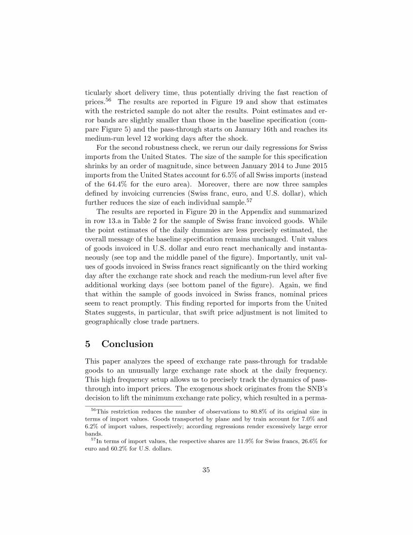
ticularly short delivery time, thus potentially driving the fast reaction ofprices.56 The results are reported in Figure 19 and show that estimateswith the restricted sample do not alter the results. Point estimates and er-ror bands are slightly smaller than those in the baseline specification (com-pare Figure 5) and the pass-through starts on January 16th and reaches itsmedium-run level 12 working days after the shock.

For the second robustness check, we rerun our daily regressions for Swissimports from the United States. The size of the sample for this specificationshrinks by an order of magnitude, since between January 2014 to June 2015imports from the United States account for 6.5% of all Swiss imports (insteadof the 64.4% for the euro area). Moreover, there are now three samplesdefined by invoicing currencies (Swiss franc, euro, and U.S. dollar), whichfurther reduces the size of each individual sample.57

The results are reported in Figure 20 in the Appendix and summarizedin row 13.a in Table 2 for the sample of Swiss franc invoiced goods. Whilethe point estimates of the daily dummies are less precisely estimated, theoverall message of the baseline specification remains unchanged. Unit valuesof goods invoiced in U.S. dollar and euro react mechanically and instanta-neously (see top and the middle panel of the figure). Importantly, unit val-ues of goods invoiced in Swiss francs react significantly on the third workingday after the exchange rate shock and reach the medium-run level after fiveadditional working days (see bottom panel of the figure). Again, we findthat within the sample of goods invoiced in Swiss francs, nominal pricesseem to react promptly. This finding reported for imports from the UnitedStates suggests, in particular, that swift price adjustment is not limited togeographically close trade partners.

5 Conclusion

This paper analyzes the speed of exchange rate pass-through for tradablegoods to an unusually large exchange rate shock at the daily frequency.This high frequency setup allows us to precisely track the dynamics of pass-through into import prices. The exogenous shock originates from the SNB’sdecision to lift the minimum exchange rate policy, which resulted in a perma-

56This restriction reduces the number of observations to 80.8% of its original size interms of import values. Goods transported by plane and by train account for 7.0% and6.2% of import values, respectively; according regressions render excessively large errorbands.

57In terms of import values, the respective shares are 11.9% for Swiss francs, 26.6% foreuro and 60.2% for U.S. dollars.

35

nent appreciation of the Swiss franc of more than 11% against the euro. Ourmain findings are twofold. First, the pass-through is immediate and com-plete for goods invoiced in euro. This finding is consistent with the view thatno systematic nominal price adjustment takes place for imports invoiced inforeign currency, as shown by Gopinath et al. (2010) and Gopinath (2015).We thus generalize these earlier findings to the case of a small open econ-omy and to a large shock. Second, for goods invoiced in Swiss francs thepass-through is partial and particularly fast: it starts on the second workingday after the exchange rate shock and reaches the medium-run pass-throughafter eight working days. Although the rate of pass-through is not uniformacross various subsets of product groups, we show that the speed of ad-justment is broadly homogenous. In our interpretation, this second findingconstitutes evidence in favor of fast nominal price adjustment.

Formulating the synthesis of both findings, we suggest that whenever afirm adjusted its border price in reaction to the large exchange rate shock,it did so very quickly. We view this fact as a novelty and as our maincontribution to the literature. We further argue that it suggests that nominalrigidities unravel quickly in the face of large exchange rate shocks.

Our results have two important implications. First, international firmsseem to demonstrate a high level of price flexibility in their ability to respondto large sudden changes in their operating environment. Our findings thustend to support state-dependent pricing models by Dotsey et al. (1999) asopposed to time-dependent pricing models by Calvo (1983). Second, priceadjustments seem to strongly depend on the nature of the exchange rateshock. Past literature has often focused on price adjustment in responseto frequent and small exchange rate shocks, showing that the pass-throughtends to be slow. Instead, we document the opposite image: a fast pass-through is uncovered for large shocks. These observations may turn out tobe crucial for the modeling of price setting behavior and the forecasting ofimport and export prices in an economic environment characterized by largeshocks.

36

References

Alessandria, G., S. Pratap, and V. Yue (2015). Export growth and aggregatedynamics in large devaluations. Mimeo.

Alvarez, F., F. Lippi, and J. Passadore (2016). Are state and time dependentmodels really different? In NBER Macroeconomics Annual 2016, Volume31. University of Chicago Press.

Amiti, M., O. Itskhoki, and J. Konings (2014). Importers, exporters, andexchange rate disconnect. American Economic Review 104 (7), 1942–78.

Amiti, M. and D. Weinstein (2011). Exports and financial shocks. QuarterlyJournal of Economics 126 (4), 1841–1877.

Auer, R., T. Chaney, and P. Saure (2014). Quality pricing-to-market. CEPRDiscussion Paper No. DP10053 .

Auer, R. and R. Schoenle (2016). Market structure and exchange rate pass-through. Journal of International Economics 98 (C), 60–77.

Bacchetta, P. and E. Van Wincoop (2005). A theory of the currency denom-ination of international trade. Journal of International Economics 67 (2),295–319.

Bakhshi, H., H. Khan, and B. Rudolf (2007). The phillips curve under state-dependent pricing. Journal of Monetary Economics 54 (8), 2321–2345.

Berman, N., P. Martin, and T. Mayer (2012). How do different exportersreact to exchange rate changes? Quarterly Journal of Economics 127 (1),437–492.

BIS (2014). Trade finance: developments and issues. CGFS Papers 50.

Burstein, A., M. Eichenbaum, and S. Rebelo (2005). Large devaluations andthe real exchange rate. Journal of Political Economy 113 (4), 742–784.

Burstein, A. and N. Jaimovich (2012). Understanding movements in aggre-gate and product-level real exchange rates. Mimeo.

Calvo, G. (1983). Staggered prices in a utility-maximizing framework. Jour-nal of Monetary Economics 12 (3), 383–398.

Campa, J. M. and L. Goldberg (2005). Exchange rate pass-through intoimport prices. Review of Economics and Statistics 87 (4), 679–690.

37

Chen, N. and L. Juvenal (2016, May). Quality, trade, and exchange ratepass-through. Journal of International Economics 100, 61–80.

Chen, Y.-C. and K. Rogoff (2003). Commodity currencies. Journal of in-ternational Economics 60 (1), 133–160.

Chung, W. (2016). Imported inputs and invoicing currency choice: Theoryand evidence from uk transaction data. Journal of International Eco-nomics 99, 237–250.

Correia, S. (2015). REGHDFE: Stata module to perform linearor instrumental-variable regression absorbing any number of high-dimensional fixed effects. Statistical Software Components, Boston Col-lege Department of Economics.

Corsetti, G., L. Dedola, and S. Leduc (2008). High exchange-rate volatilityand low pass-through. Journal of Monetary Economics 55 (6), 1113–1128.

Cravino, J. and A. Levchenko (2015). The distributional consequences oflarge devaluations. Mimeo.

Devereux, M., B. Tomlin, and W. Dong (2015). Exchange rate pass-through,currency of invoicing and market share. Working paper 21413, NationalBureau of Economic Research.

Dixit, A. (1989). Hysteresis, import penetration, and exchange rate pass-through. Quarterly Journal of Economics, 205–228.

Dotsey, M., R. King, and A. Wolman (1999). State-dependent pricing andthe general equilibrium dynamics of money and output. Quarterly Journalof Economics, 655–690.

Efing, M., R. Fahlenbrach, C. Herpfer, and P. Krueger (2015). How doinvestors and firms react to an unexpected currency appreciation shock?Swiss Finance Institute Research Paper (15-65).

Egger, P. and A. Lassmann (2015). The causal impact of common nativelanguage on international trade: evidence from a spatial regression dis-continuity design. The Economic Journal 125 (584), 699–745.

Enders, Z., G. Muller, and A. Scholl (2011). How do fiscal and technologyshocks affect real exchange rates?: New evidence for the United States.Journal of International Economics 83 (1), 53–69.

38

Engel, C. (2006). Equivalence results for optimal pass-through, optimalindexing to exchange rates, and optimal choice of currency for exportpricing. Journal of the European Economic Association 4 (6), 1249–1260.

Engel, C. and K. West (2005). Exchange rates and fundamentals. Journalof Political Economy 113 (3), 485–517.

Feenstra, R. (1989). Symmetric pass-through of tariffs and exchange ratesunder imperfect competition: An empirical test. Journal of InternationalEconomics 27 (1), 25–45.

Feltrin, C. and B. Guimaraes (2015). Time-dependent or state-dependentpricing? Evidence from a large devaluation episode. Brazilian Review ofEconometrics. Forthcoming.

Flach, L. (2016). Quality upgrading and price heterogeneity: evidence fromBrazilian exporters. Journal of International Economics.

Forbes, K., I. M. Hjortsoe, and T. Nenova (2015). The shocks matter:improving our estimates of exchange rate pass-through. External MPCUnit Discussion Paper (43).

Gagnon, E. (2009). Price setting during low and high inflation: evidencefrom Mexico. Quarterly Journal of Economics 124 (3), 1221–1263.

Gagnon, E., B. R. Mandel, and R. J. Vigfusson (2014). Missing importprice changes and low exchange rate pass-through. American EconomicJournal: Macroeconomics 6 (2), 156–206.

Goldberg, L. and C. Tille (2008). Vehicle currency use in international trade.Journal of International Economics 76 (2), 177–192.

Golosov, M. and R. Lucas (2007). Menu costs and phillips curves. Journalof Political Economy 115 (2), 171–199.

Gopinath, G. (2015). The international price system. Working Paper 21646,National Bureau of Economic Research.

Gopinath, G., O. Itskhoki, and R. Rigobon (2010). Currency choice andexchange rate pass-through. American Economic Review 100 (1), 304–336.

Gopinath, G. and R. Rigobon (2008). Sticky borders. Quarterly Journal ofEconomics, 531–575.

39

Gorodnichenko, Y. and O. Talavera (2016). Price setting in online mar-kets: Basic facts, international comparisons, and cross-border integration.American Economic Review . Forthcoming.

Grinberg, F. (2015). Large currency depreciations and menu costs. Mimeo.

Kropf, A. and P. Saure (2014). Fixed costs per shipment. Journal of Inter-national Economics 92 (1), 166–184.

Mankiw, G. and R. Reis (2002). Sticky information versus sticky prices:a proposal to replace the New Keynesian Phillips curve. The QuarterlyJournal of Economics 117 (4), 1295–1328.

Meese, R. and K. Rogoff (1988). Was it real? the exchange rate-interestdifferential relation over the modern floating-rate period. Journal of Fi-nance, 933–948.

Menon, J. (1995). Exchange rate pass-through. Journal of Economic Sur-veys 9 (2), 197–231.

Mirkov, N., I. Pozdeev, and P. Soderlind (2015, November). Did marketsanticipate the removal of the Swiss franc cap? Mimeo.

Nakamura, E. and J. Steinsson (2008). Five facts about prices: a reeval-uation of menu cost models. Quarterly Journal of Economics 123 (4),1415–1464.

Neiman, B. (2010). Stickiness, synchronization, and pass-through in in-trafirm trade prices. Journal of Monetary Economics 57 (3), 295–308.

Rauch, J. E. (1999). Networks versus markets in international trade. Journalof international Economics 48 (1), 7–35.

SNB (2015). Business cycle trends. Swiss National Bank quarterly bul-letin (1), 30–33.

Vavra, J. S. (2013). Inflation dynamics and time-varying volatility: Newevidence and an ss interpretation. Technical report, National Bureau ofEconomic Research.

Verhoogen, E. (2008). Trade, quality upgrading, and wage inequality in theMexican manufacturing sector. Quarterly Journal of Economics, 489–530.

40

Appendix 1: Tables

Table 4: Shares of invoicing currency for imports from the euro areaby 2-digit HS code

Based on transactions Based on value

2-digit HS codeShare in tot.imports [%]

Invoicing currencyshares

Share in tot.imports [%]

Invoicing currencyshares

CHF EURO Other CHF EURO Other

01 0.08 0.16 0.84 0.00 0.08 0.11 0.89 0.00

02 0.39 0.13 0.87 0.00 0.29 0.12 0.87 0.01

03 0.45 0.06 0.92 0.02 0.21 0.09 0.87 0.04

04 0.56 0.05 0.95 0.00 0.47 0.04 0.96 0.00

05 0.05 0.25 0.74 0.00 0.04 0.03 0.97 0.00

06 1.36 0.32 0.68 0.00 0.47 0.23 0.77 0.00

07 1.84 0.17 0.83 0.00 0.43 0.14 0.86 0.00

08 0.86 0.13 0.87 0.00 0.54 0.06 0.93 0.01

09 0.26 0.18 0.82 0.00 0.13 0.06 0.92 0.02

10 0.12 0.24 0.76 0.00 0.21 0.46 0.54 0.00

11 0.11 0.08 0.92 0.00 0.07 0.04 0.96 0.00

12 0.33 0.33 0.67 0.00 0.16 0.29 0.71 0.00

13 0.03 0.20 0.79 0.01 0.04 0.07 0.90 0.03

14 0.01 0.11 0.89 0.00 0.00 0.18 0.81 0.01

15 0.20 0.19 0.81 0.00 0.16 0.07 0.91 0.02

16 0.37 0.18 0.80 0.01 0.20 0.27 0.70 0.03

17 0.50 0.29 0.70 0.00 0.19 0.13 0.86 0.01

18 0.91 0.71 0.29 0.00 0.37 0.36 0.47 0.18

19 1.55 0.24 0.75 0.00 0.59 0.22 0.78 0.00

20 0.83 0.20 0.80 0.00 0.28 0.16 0.81 0.02

21 1.48 0.56 0.44 0.00 0.45 0.18 0.82 0.00

22 1.50 0.25 0.75 0.00 1.36 0.16 0.83 0.00

23 0.29 0.29 0.71 0.00 0.24 0.26 0.72 0.02

24 0.06 0.58 0.36 0.06 0.09 0.17 0.36 0.47

25 0.56 0.22 0.77 0.00 0.33 0.28 0.72 0.01

26 0.04 0.02 0.98 0.00 0.02 0.09 0.91 0.00

27 0.39 0.35 0.64 0.01 7.42 0.73 0.25 0.01

28 0.36 0.32 0.67 0.01 0.35 0.15 0.84 0.02

29 0.63 0.43 0.55 0.02 7.89 0.75 0.22 0.02

30 0.88 0.32 0.67 0.01 13.19 0.31 0.68 0.01

31 0.06 0.24 0.76 0.00 0.09 0.20 0.80 0.01

32 0.92 0.24 0.75 0.00 0.65 0.15 0.85 0.00

33 1.66 0.42 0.58 0.00 0.81 0.29 0.70 0.01

34 1.10 0.29 0.71 0.00 0.43 0.15 0.84 0.00

35 0.27 0.24 0.76 0.00 0.16 0.10 0.90 0.00

36 0.01 0.22 0.76 0.01 0.02 0.05 0.94 0.01

37 0.06 0.28 0.70 0.02 0.04 0.26 0.72 0.02

38 1.58 0.29 0.70 0.01 1.00 0.26 0.71 0.03

39 5.63 0.27 0.73 0.01 4.38 0.13 0.86 0.00

40 1.64 0.36 0.62 0.02 0.79 0.32 0.68 0.00

41 0.04 0.11 0.89 0.00 0.06 0.03 0.97 0.00

42 1.44 0.36 0.63 0.01 0.48 0.23 0.71 0.06

43 0.04 0.33 0.67 0.01 0.02 0.33 0.65 0.02

44 1.26 0.21 0.79 0.00 1.33 0.14 0.86 0.00

45 0.03 0.20 0.79 0.01 0.03 0.11 0.88 0.00

46 0.05 0.20 0.80 0.00 0.00 0.10 0.89 0.00

47 0.07 0.03 0.97 0.01 0.07 0.00 0.93 0.07

48 2.21 0.25 0.75 0.00 1.59 0.21 0.79 0.00

49 3.34 0.50 0.49 0.01 1.24 0.31 0.69 0.00

50 0.03 0.13 0.86 0.00 0.01 0.04 0.96 0.00

Continued on next page

41

Table 4 – continued from previous page

Based on transactions Based on value

2-digit HS codeShare in tot.imports [%]

Invoicing currencyshares

Share in tot.imports [%]

Invoicing currencyshares

CHF EURO Other CHF EURO Other

51 0.09 0.15 0.84 0.01 0.07 0.06 0.94 0.00

52 0.20 0.20 0.80 0.00 0.12 0.32 0.68 0.00

53 0.05 0.21 0.79 0.00 0.01 0.22 0.78 0.00

54 0.16 0.17 0.83 0.00 0.13 0.07 0.93 0.00

55 0.13 0.20 0.80 0.00 0.06 0.08 0.88 0.05

56 0.32 0.19 0.81 0.00 0.17 0.07 0.92 0.00

57 0.33 0.33 0.67 0.00 0.10 0.30 0.70 0.00

58 0.19 0.23 0.77 0.00 0.04 0.15 0.85 0.00

59 0.20 0.26 0.74 0.00 0.11 0.19 0.81 0.00

60 0.11 0.09 0.91 0.00 0.05 0.05 0.95 0.00

61 4.26 0.35 0.65 0.00 0.52 0.31 0.68 0.01

62 3.77 0.34 0.66 0.00 0.72 0.23 0.75 0.01

63 1.23 0.32 0.67 0.00 0.28 0.16 0.84 0.00

64 2.16 0.27 0.72 0.00 0.59 0.16 0.82 0.02

65 0.27 0.37 0.63 0.00 0.04 0.19 0.81 0.01

66 0.07 0.27 0.73 0.00 0.01 0.19 0.81 0.00

67 0.10 0.33 0.67 0.00 0.01 0.35 0.64 0.01

68 1.01 0.20 0.80 0.00 0.65 0.17 0.82 0.00

69 0.84 0.18 0.81 0.00 0.39 0.12 0.88 0.00

70 1.26 0.37 0.62 0.01 0.70 0.15 0.84 0.00

71 0.55 0.35 0.64 0.01 3.74 0.31 0.64 0.05

72 0.88 0.22 0.78 0.00 1.98 0.16 0.84 0.00

73 3.98 0.28 0.71 0.01 2.44 0.12 0.88 0.00

74 0.40 0.24 0.75 0.01 0.73 0.11 0.85 0.04

75 0.01 0.13 0.85 0.02 0.05 0.04 0.95 0.01

76 1.07 0.19 0.81 0.01 1.62 0.12 0.87 0.01

78 0.01 0.29 0.71 0.00 0.01 0.02 0.98 0.00

79 0.04 0.22 0.75 0.02 0.04 0.21 0.61 0.18

80 0.01 0.26 0.73 0.00 0.01 0.09 0.82 0.09

81 0.05 0.18 0.80 0.02 0.08 0.06 0.89 0.05

82 1.73 0.30 0.70 0.00 0.64 0.15 0.85 0.00

83 1.21 0.33 0.66 0.01 0.49 0.19 0.80 0.00

84 9.21 0.28 0.70 0.02 10.32 0.14 0.83 0.03

85 9.59 0.35 0.63 0.02 5.71 0.22 0.75 0.03

86 0.08 0.11 0.89 0.00 0.59 0.10 0.90 0.00

87 4.60 0.54 0.45 0.02 8.49 0.60 0.39 0.00

88 0.10 0.10 0.58 0.32 0.49 0.11 0.38 0.50

89 0.01 0.14 0.85 0.01 0.06 0.03 0.95 0.02

90 3.86 0.37 0.61 0.01 3.52 0.26 0.72 0.02

91 0.40 0.36 0.63 0.01 1.28 0.27 0.72 0.01

92 0.11 0.36 0.64 0.00 0.04 0.31 0.68 0.01

93 0.03 0.12 0.88 0.00 0.07 0.13 0.86 0.00

94 4.33 0.17 0.82 0.00 2.73 0.12 0.88 0.01

95 1.55 0.51 0.49 0.00 0.35 0.21 0.78 0.01

96 1.04 0.29 0.70 0.00 0.30 0.37 0.62 0.00

min 0.01 0.02 0.29 0.00 0.00 0.00 0.22 0.00

max 9.59 0.71 0.98 0.32 13.19 0.75 0.98 0.50

mean 1.05 0.26 0.73 0.01 1.05 0.19 0.79 0.03

median 0.39 0.24 0.75 0.00 0.28 0.16 0.83 0.01

Note: the corresponding descriptions for the 2-digit HS codes can be found athttp://xtares.admin.ch/tares/main/mainFormFiller.do;jsessionid=ng6ZXMrTJNhpKyd6TPZv3MGkLGzs8qTTqhbkv48GL7Cfs4Qn2XVL!91241224.

42

Appendix 2: Currency switching and the exchangerate shock

This Appendix presents information on whether the pass-through estimatesare biased because of currency invoice switching at the time of the exchangerate shock. It is argued in Gopinath et al. (2010) that in the face of smallfrictions, currency invoice switching should not occur. In the figure below,we show that the Gopinath et al. (2010) claim holds in the face of largeshocks for Swiss imports. Two panels for the number of transactions andtheir value are presented. Each of these panels are shaded as follows: thedark area is the share of euro-invoicing, light is the share of Swiss francinvoicing, light grey is the share of switching from Swiss franc to euro-invoicing after January 15, 2015, and grey is the share of switching fromeuro to Swiss franc invoicing after January 15, 2015. A switch in currencyinvoicing for a firm is proxied by the triplet: postal code, HS product, andpartner country.

The results show that the level of switching after January 15, 2015 isparticularly low. It is less than 0.01% for both categories. Further, thesmall degree of switching in the invoice currencies occurs in both directions,suggesting that the effect is neutral at best. From this we conclude that ourdaily pass-through estimates are not subject to switching effects at the timeof the exchange rate shock.

43

Figure 8: Currency switching in 2015 - swiss imports from the euro area

.28

.3.3

2.3

4

2014 2014.5 2015 2015.5 2016date

Based on transactions

.2.2

4.2

8.3

2.3

6

2014 2014.5 2015 2015.5 2016date

Based on values

Only EUR EUR, only CHF in 2014CHF, only EUR in 2014 Only CHF

The dark area is the share of euro invoicing, light is the share of Swiss franc invoicing, light gray area isthe share of switching from Swiss franc to euro invoicing after January 15, 2015, and gray is the share ofswitching from euro to Swiss franc invoicing after January 15, 2015.

44

Appendix 3: Graphs to the robustness checks

4.2 Graphs for proxying firm size

-.3-.2-.10.1log change

16 J

an 2

015

31 J

an 2

015

14 F

eb 2

015

28 F

eb 2

015

date

EU

R in

voic

ed

Sta

rt o

f adj

.Ja

n 20

End

of a

dj.

Jan

27

-.2-.15-.1-.050.05log change

16 J

an 2

015

31 J

an 2

015

14 F

eb 2

015

28 F

eb 2

015

date

CH

F in

voic

ed

Dai

ly r

eact

ion

of im

port

uni

t val

ues

(big

exp

orte

rs)

daily

dum

mie

seu

rchf

log-

diff.

with

Jan

15fo

llow

ing

mon

ths

Fig

ure

9:

Dai

lyd

um

mie

sfo

rim

por

tu

nit

valu

esfr

omb

igH

S-c

ountr

yex

por

tco

mb

i-n

atio

ns

(sp

ecifi

cati

on

2).

Th

ere

gre

ssio

nin

clu

des

augm

ente

dH

S-p

osta

lco

de-

cou

ntr

ytr

iple

tsfi

xed

-eff

ects

and

a2-d

igit

HS

-cou

ntr

ysp

ecifi

ctr

end

.E

rror

are

clust

ered

atth

ep

ost

alco

de

leve

l.

45

-.3-.2-.10.1log change

16 J

an 2

015

31 J

an 2

015

14 F

eb 2

015

28 F

eb 2

015

date

EU

R in

voic

ed

Sta

rt a

nd e

nd o

f adj

.Ja

n 30

-.2-.10.1log change

16 J

an 2

015

31 J

an 2

015

14 F

eb 2

015

28 F

eb 2

015

date

CH

F in

voic

ed

Dai

ly r

eact

ion

of im

port

uni

t val

ues

(big

impo

rter

s)

daily

dum

mie

seu

rchf

log-

diff.

with

Jan

15fo

llow

ing

mon

ths

Fig

ure

10:

Dail

yd

um

mie

sfo

rim

por

tu

nit

valu

esof

big

HS

-pos

tal

cod

eim

por

ter

com

bin

ati

ons

(sp

ecifi

cati

on2)

.T

he

regre

ssio

nin

clu

des

au

gmen

ted

HS

-pos

tal

cod

e-co

untr

ytr

iple

tsfi

xed

-eff

ects

and

a2-

dig

itH

S-c

ou

ntr

ysp

ecifi

ctr

end

.E

rror

are

clu

ster

edat

the

pos

tal

cod

ele

vel.

46

-.2-.15-.1-.050.05log change

16 J

an 2

015

31 J

an 2

015

14 F

eb 2

015

28 F

eb 2

015

date

EU

R in

voic

ed

Sta

rt o

f adj

.Ja

n 19

End

of a

dj.

Jan

26

-.2-.15-.1-.050.05log change

16 J

an 2

015

31 J

an 2

015

14 F

eb 2

015

28 F

eb 2

015

date

CH

F in

voic

ed

Dai

ly r

eact

ion

of im

port

uni

t val

ues

(val

ue <

300

)

daily

dum

mie

seu

rchf

log-

diff.

with

Jan

15fo

llow

ing

mon

ths

Fig

ure

11:

Dai

lyd

um

mie

sfo

rim

por

tu

nit

valu

esfo

rsh

ipm

ents

wor

thle

ssth

anC

HF

300

(sp

ecifi

cati

on2)

.T

he

regr

essi

onin

clu

des

augm

ente

dH

S-p

osta

lco

de-

cou

ntr

ytr

iple

tsfi

xed

-eff

ects

and

a2-

dig

itH

S-c

ountr

ysp

ecifi

ctr

end

.E

rror

sar

ecl

ust

ered

atth

ep

osta

lco

de

leve

l.

47

-.2-.15-.1-.050.05log change

16 J

an 2

015

31 J

an 2

015

14 F

eb 2

015

28 F

eb 2

015

date

EU

R in

voic

ed

Sta

rt o

f adj

.Ja

n 20

End

of a

dj.

Jan

27

-.2-.15-.1-.050.05log change

16 J

an 2

015

31 J

an 2

015

14 F

eb 2

015

28 F

eb 2

015

date

CH

F in

voic

ed

Dai

ly r

eact

ion

of im

port

uni

t val

ues

(val

ue >

300

)

daily

dum

mie

seu

rchf

log-

diff.

with

Jan

15fo

llow

ing

mon

ths

Fig

ure

12:

Daily

du

mm

ies

for

imp

ort

un

itva

lues

for

ship

men

tsw

orth

mor

eth

anC

HF

300

(sp

ecifi

cati

on

2).

Th

ere

gre

ssio

nin

clu

des

augm

ente

dH

S-p

osta

lco

de-

cou

ntr

ytr

iple

tsfi

xed

-eff

ects

and

a2-

dig

itH

S-c

ountr

ysp

ecifi

ctr

end

.E

rrors

are

clu

ster

edat

the

post

alco

de

leve

l.

48

4.3 Graphs for intermediate, investment and consumption goods

-.2-.15-.1-.050.05log change

16 J

an 2

015

31 J

an 2

015

14 F

eb 2

015

28 F

eb 2

015

date

EU

R in

voic

ed

Sta

rt o

f adj

.Ja

n 19

End

of a

dj.

Jan

26

-.2-.15-.1-.050.05log change

16 J

an 2

015

31 J

an 2

015

14 F

eb 2

015

28 F

eb 2

015

date

CH

F in

voic

ed

Dai

ly r

eact

ion

of im

port

uni

t val

ues

(con

sum

ptio

n go

ods)

daily

dum

mie

seu

rchf

log-

diff.

with

Jan

15fo

llow

ing

mon

ths

Fig

ure

13:

Dai

lyd

um

mie

sfo

rim

por

tu

nit

valu

esfo

rco

nsu

mp

tion

good

s(s

pec

ifica

tion

2).

Th

ere

gres

sion

incl

ud

esau

gmen

ted

HS

-pos

talco

de-

cou

ntr

ytr

iple

tsfi

xed

-eff

ects

and

a2-

dig

itH

S-c

ountr

ysp

ecifi

ctr

end

.E

rror

sar

ecl

ust

ered

atth

ep

osta

lco

de

leve

l.

49

-.2-.15-.1-.050.05log change

16 J

an 2

015

31 J

an 2

015

14 F

eb 2

015

28 F

eb 2

015

date

EU

R in

voic

ed

Sta

rt o

f adj

.Ja

n 22

End

of a

dj.

Jan

27

-.2-.15-.1-.050.05log change

16 J

an 2

015

31 J

an 2

015

14 F

eb 2

015

28 F

eb 2

015

date

CH

F in

voic

ed

Dai

ly r

eact

ion

of im

port

uni

t val

ues

(raw

and

inve

st. g

oods

)

daily

dum

mie

seu

rchf

log-

diff.

with

Jan

15fo

llow

ing

mon

ths

Fig

ure

14:

Dai

lyd

um

mie

sfo

rim

por

tu

nit

valu

esfo

rin

vest

men

tgo

od

san

dra

wm

ater

ials

(sp

ecifi

cati

on2).

Th

ere

gre

ssio

nin

clu

des

augm

ente

dH

S-p

osta

lco

de-

cou

ntr

ytr

iple

tsfi

xed

-eff

ects

and

a2-

dig

itH

S-c

ountr

ysp

ecifi

ctr

end

.E

rrors

are

clu

ster

edat

the

post

alco

de

leve

l.

50

-.2-.15-.1-.050.05log change

16 J

an 2

015

31 J

an 2

015

14 F

eb 2

015

28 F

eb 2

015

date

EU

R in

voic

ed

Sta

rt o

f adj

.Ja

n 19

End

of a

dj.

Jan

23

-.2-.15-.1-.050.05log change

16 J

an 2

015

31 J

an 2

015

14 F

eb 2

015

28 F

eb 2

015

date

CH

F in

voic

ed

Dai

ly r

eact

ion

of im

port

uni

t val

ues

(inte

rm. g

oods

)

daily

dum

mie

seu

rchf

log-

diff.

with

Jan

15fo

llow

ing

mon

ths

Fig

ure

15:

Dail

yd

um

mie

sfo

rim

por

tu

nit

valu

esfo

rin

term

edia

tego

od

s(s

pec

ifica

tion

2).

Th

ere

gres

sion

in-

clu

des

au

gmen

ted

HS

-post

alco

de-

cou

ntr

ytr

iple

tsfi

xed

-eff

ects

and

a2-

dig

itH

S-c

ountr

ysp

ecifi

ctr

end

.E

rror

sar

ecl

ust

ered

atth

ep

ost

alco

de

leve

l.

51

4.4 Graphs by Rauch classification

-.2-.15-.1-.050.05log change

16 J

an 2

015

31 J

an 2

015

14 F

eb 2

015

28 F

eb 2

015

date

EU

R in

voic

ed

Sta

rt o

f adj

.Ja

n 19

End

of a

dj.

Jan

27

-.2-.15-.1-.050.05log change

16 J

an 2

015

31 J

an 2

015

14 F

eb 2

015

28 F

eb 2

015

date

CH

F in

voic

ed

Dai

ly r

eact

ion

of im

port

uni

t val

ues

(diff

eren

tiate

d go

ods)

daily

dum

mie

seu

rchf

log-

diff.

with

Jan

15fo

llow

ing

mon

ths

Fig

ure

16:

Dai

lyd

um

mie

sfo

rim

por

tu

nit

valu

esof

diff

eren

tiate

dgo

od

s(s

pec

ifica

-ti

on

2).

Th

ere

gres

sion

incl

ud

esau

gmen

ted

HS

-pos

tal

cod

e-co

untr

ytr

iple

tsfi

xed

-eff

ects

and

a2-

dig

itH

S-c

ountr

ysp

ecifi

ctr

end

.E

rror

are

clu

ster

edat

the

pos

tal

cod

ele

vel.

52

4.5 Graphs for single item declarations

-.3-.2-.10.1log change

16 J

an 2

015

31 J

an 2

015

14 F

eb 2

015

28 F

eb 2

015

date

EU

R in

voic

ed

Sta

rt a

nd e

nd o

f adj

.Ja

n 19

-.2-.15-.1-.050.05log change

16 J

an 2

015

31 J

an 2

015

14 F

eb 2

015

28 F

eb 2

015

date

CH

F in

voic

ed

Dai

ly r

eact

ion

of im

port

uni

t val

ues

(sin

gle

item

)

daily

dum

mie

seu

rchf

log-

diff.

with

Jan

15fo

llow

ing

mon

ths

Fig

ure

17:

Dai

lyd

um

mie

sfo

rim

por

tu

nit

valu

esw

hen

the

tran

sact

ion

isu

niq

ue

inth

ecu

stom

dec

lara

tion

(sp

ecifi

cati

on2)

.T

he

regr

essi

onin

clu

des

au

gm

ente

dH

S-

pos

tal

cod

e-co

untr

ytr

iple

tsfi

xed

-eff

ects

and

a2-

dig

itH

S-c

ountr

ysp

ecifi

ctr

end

.E

rror

are

clu

ster

edat

the

pos

tal

cod

ele

vel.

53

4.6 Graphs for section-level regressions

-.3-.2-.10.1log change

16 J

an 2

015

31 J

an 2

015

14 F

eb 2

015

28 F

eb 2

015

date

EU

R in

voic

ed

-.2-.10.1log change

16 J

an 2

015

31 J

an 2

015

14 F

eb 2

015

28 F

eb 2

015

date

CH

F in

voic

ed

Dai

ly r

eact

ion

of im

port

uni

t val

ues

(med

ian

HS

sec

tion)

daily

dum

mie

seu

rchf

log-

diff.

with

Jan

15fo

llow

ing

mon

ths

Fig

ure

18:

Med

ian

ofea

chH

Sse

ctio

nsp

ecifi

cd

aily

coeffi

cien

tson

imp

ort

un

itva

lues

(sp

ecifi

cati

on2)

.T

he

regr

essi

onin

clu

des

au

gm

ente

dH

S-p

osta

lco

de-

cou

ntr

ytr

iple

tsfi

xed

-eff

ects

and

aco

untr

ysp

ecifi

ctr

end

.E

rror

sare

clu

ster

edat

the

pos

tal

cod

ele

vel.

54

4.7 Graphs for distance related regressions

-.2-.15-.1-.050log change

16 J

an 2

015

31 J

an 2

015

14 F

eb 2

015

28 F

eb 2

015

date

EU

R in

voic

ed

Sta

rt o

f adj

.Ja

n 16

End

of a

dj.

Feb

2

-.2-.15-.1-.050.05log change

16 J

an 2

015

31 J

an 2

015

14 F

eb 2

015

28 F

eb 2

015

date

CH

F in

voic

ed

Dai

ly r

eact

ion

of im

port

uni

t val

ues

- tr

ansp

ort b

y tr

ansp

orte

d vi

a ro

ad

daily

dum

mie

seu

rchf

log-

diff.

with

Jan

15fo

llow

ing

mon

ths

Fig

ure

19:

Dai

lydu

mm

ies

for

imp

ort

un

itva

lues

(sp

ecifi

cati

on2)

.T

he

sam

ple

incl

udes

only

imp

ort

str

an

sport

edvia

road

.T

he

regr

essi

onin

clu

des

augm

ente

dH

S-p

osta

lco

de-

cou

ntr

ytr

iple

tsfi

xed

-eff

ects

and

a2-

dig

itH

S-

cou

ntr

ysp

ecifi

ctr

end

.E

rror

sare

clu

ster

edat

the

pos

tal

cod

ele

vel.

55

Figure 20: Daily reaction of import unit values - trade with the US-.

3-.

2-.

10

.1.2

log

chan

ge

16 Jan 2015 31 Jan 2015 14 Feb 2015 28 Feb 2015date

USD invoiced

-.3

-.2

-.1

0.1

log

chan

ge

16 Jan 2015 31 Jan 2015 14 Feb 2015 28 Feb 2015date

EUR invoiced

Start of adj.Jan 20

End of adj.Jan 27

-.2

-.1

0.1

.2lo

g ch

ange

16 Jan 2015 31 Jan 2015 14 Feb 2015 28 Feb 2015date

CHF invoiced

daily dummies usdchf log-diff. with Jan15 following months

Daily dummies for import unit values (specification 2). The sample includes only importsfrom the USA to Switzerland. The regression includes augmented HS-postal code-countrytriplets fixed-effects and a 2-digit HS-country specific trend. Errors are clustered at thepostal code level.

56

Appendix 4: Standard estimation procedure

Traditional estimates of pass-through into export prices typically take theform

∆pij,t =

L∑l=0

βl∆ej,t + Zij,tγ + uij,t (3)

where ∆pij,t denotes the change in the price of good i exported from a givencountry C to country j, at time t, ∆ej,t denotes the change in the exchangerate of country C’s and country j’s currencies, Zij,t is a set of potentiallycountry- and good-specific control variables and uij,t is an error term.

Estimations of this specification crucially rely on the underlying assump-tion that the error term is uncorrelated with the independent variables, thatis, E[∆ej,t−luij,t] = 0 holds for all lags included. If this condition is violated,the estimates suffer from endogeneity bias.

In the following paragraphs, we argue that the crucial assumption maybe violated through a number effects and mechanisms described by the lit-erature.

Endogeneity would occur if the theoretical price parity condition holds,as the exchange rate and prices should be jointly determined. Although thisviolation is usually rejected because exchange rate and prices are not foundto be cointegrated (see e.g. Campa and Goldberg (2005)), other sources ofendogeneity exist and imperfect measurement or omitted variables are likelyto affect the estimation. Corsetti et al. (2008), for example, stress the needto correctly control for marginal cost and demand.

In an early paper, Meese and Rogoff (1988) conjecture that real shocks(such as productivity shocks) drive real exchange rate changes. Relatedly,Enders et al. (2011) present evidence that productivity shocks induce appre-ciations of the real exchange rate. Thus, real shocks may actually drive inno-vations in the exchange rate and, simultaneously, innovations in producer’scost. If the marginal cost cannot be adequately controlled for, omitting thisvariable results in biased estimates because E[∆ej,tuij,t] 6= 0 if prices adaptinstantaneously and E[∆ej,tuij,t+l] 6= 0 (l > 0) if they adjust sluggishly.

Engel and West (2005) take a different approach by stressing the asset-price nature of exchange rates. The authors suggest that exchange ratesdepend on expectations of future fundamentals, arguing, in particular, thatinnovations in the exchange rates should be correlated with news aboutfuture fundamentals. Empirically, they find evidence that exchange rates

57

Granger-cause fundamentals. In such a setting, an anticipated technologicalshock impacts the exchange rate at time t, and producer’s cost at time t+ l.Here again, if the marginal cost cannot be correctly controlled for, uij,t and∆ej,t may both react to the same shock, implying that E[ej,t−luij,t] = ηl 6= 0

for a lag l > 0.58

To frame these arguments formally, consider the following OLS estimatorof (β′, γ′)′ in (3): (

β

γ

)=

(β

γ

)+

(e′e e′Z

Z ′e Z ′Z

)−1(e′u

Z ′u

)(4)

where e = ( ∆e0 ∆e1 ... ∆eL ) is the matrix of exchange rate lags, Z thematrix of control variables and u the error vector. Inverting the partitionedmatrix, the bias on β is given by:

β − β =

(A−A(e′Z)(Z ′)−1

)(e′u

Z ′u

)(5)

with A = (e′e − e′Z(Z ′Z)−1Z ′e)−1 = (e′Mze)−1. If all variables in Z are

exogenous, we get that plimZ′uT = 0, so that the direction of the asymptotic

bias only depends on the behavior of A and e′u.In the case that the lags of exchange rate changes are uncorrelated (for

example in the case of a random walk in the exchange rate), plimA is a diag-onal matrix whose elements are equal to plim(e′lMzel)

−1, which is positive

because Mz is positive definite. The asymptotic bias on each βl is then equal

to Alηl, where Al = plim(e′lMzel)

−1, and is thus of the same sign as ηl. If,

in addition, the error terms are autocorrelated59, the bias does not affect βlonly. For example, if uij,t = ρuij,t−1 + εt, then E[uij,t∆ej,t−l−l] = ρlηl 6= 0

follows for l > 0 so that all estimates on lags “further away” than l areinconsistent. The direction of the bias then depends on ηl and on ρ.

For a concrete example, consider a positive anticipated shock to the tech-nology of the exporting country in a world like in Engel and West (2005).

58If the marginal cost is measured with an error (e.g. proxied using expenditure sharesand price changes of input prices), the exchange rate will still be correlated with uij,t if itis also correlated with the measurement error. An other example is a shock in preferencesin the demand for the exporter’s good which would have a similarly uncontrolled effect onboth the price and the exchange rate.

59Note that using residuals derived from the inconsistent β, one might be unable todetect such autocorrelation because in this case the residuals are not a consistent estimatorof the error term.

58

In this setup, the anticipated technology shock in period t leads to an ap-preciation of the exchange rate at time t− l. Defining the exchange rate ashome currency per foreign currency, this means ∆ej,t−l < 0. At the sametime, this shock is associated with a negative shock on the price at time t(uij,t < 0). In sum, such a positive technological shock (inducing an appre-ciation of the exporter’s currency and a future reduction in costs) generatesηl > 0. A positive ρ is consistent with persistency in the shock. Overall,the bias on the lags would thus be positive, resulting in an overestimationof the delayed pass-through.

The shock to the EURCHF exchange rate used in this paper is arguablyunrelated to any shock that might produce endogeneity issues. The shockwas unrelated to any technological or taste shock, but was purely due tothe SNB’s decision. Thus, our estimates take place in a setting free ofendogeneity concerns.

59