the socio-economic gradient of child development: cross ... · rubio-codina, attanasio, meghir,...

Rubio-Codina, Attanasio, Meghir, Varela, and Grantham-McGregor – On-line Appendix

The Socio-Economic Gradient of Child Development: Cross-Sectional Evidence from Children 6-42

Months in Bogota: On-line Appendix

Appendix 1: Sampling Strategy

Residential blocks in Bogota are classified in six ‘estratos’ according to their location (such as

industrial, commercial, residential, and marginalized areas), quality of streets and pavements,

accessibility to households, and housing quality (materials of roofs and front walls, size of the

façade, parking, and garden). In practice, blocks in the same ‘estrato’ are geographically

concentrated, and separate from those in different ‘estratos’ (see Figure A1). In addition, official

administrative data from the 2005 Census and the 2011 Cadastre indicate that both family size and

fertility rates monotonically decrease by ‘estrato’. Hence, it was deemed important to sample

households in each of the first four ‘estratos’ independently in order to obtain a sample

representative of low- and middle-income levels.

We followed a three stage sampling process. First, we stratified the city by ‘estrato’ and randomly

sampled neighborhoods (primary sampling unit) within them, weighting by the proportion of women

in fertile age (13-49 years). Second, within each neighborhood, we randomly sampled three blocks

(secondary sampling unit), also weighting by the proportion of women in fertile age.1 Third, in each

selected block, we carried out a mini-census (door-to-door sampling) to identify households with

children (tertiary sampling unit) in the eligible age ranges. To ensure a uniform age distribution, we

stratified eligible children in a block in age categories: 6-14, 15-23, 24-32, and 33-41 months. Based

on the 2005 Census, we expected to find ten eligible children per block and age group on average, of

which eight were included in the study by random draw. We assumed a rejection rate of 25 percent.

Anticipating less eligible children and higher rejection rates in E4, we decided to include all children

satisfying the inclusion criteria in the blocks in this ‘estrato’. We excluded one child with mental

disabilities and one pair of twins. In addition, in the four households where there was more than one

child satisfying the inclusion criteria, we selected which to include at random.

The original sample design was balanced across age groups and ‘estrato’, with 90 children in each

stratum-age cell for a total of 1,440 children in 240 blocks. These sample sizes would allow detecting

differences of 0.415 SD of a z-score amongst stratum-age groups at 80 percent power and 5 percent

significance. However, as soon as field operations started, it was clear that households living in E4

were extremely reluctant to participate in the survey, mostly because of apparent mistrust.

Moreover, relative to the data in the 2005 Census, we found a much reduced number of children per

block. Hence, we modified the sample structure in two ways. Firstly, we increased the number of

blocks sampled. Secondly, to compensate for the loss of children in E4 we increased the number of

children in E1 and E2 by 90 each. In addition, mindful of the larger degree of heterogeneity in SES to

be found in E3, we oversampled this ‘estrato’ by adding 180 children. As a result, our new target

sample was 450 children in E1, 450 children in E2, and 540 children in E3, for a total of 1,440 children

ages 6-42 months in 240 blocks.

1 Because of budget and logistical constraints, neighborhoods and blocks with a higher proportion of women in

fertile age had a higher probability of being included in the sample.


Appendix 2: Data Collection Strategy

Once identified, all selected children in a block were assigned to one of the eight interviewers we

had trained (all female). Data was collected in two subsequent stages:

(i) Household Survey: the interviewer interviewed the biological mother of the child in the

household. The survey collected basic socio-economic information on the household and dwelling

characteristics (such as demographic composition, education level and employment status for

household members, and assets), and formal and informal child care arrangements. It also included

UNICEF’s Family Care Indicator (FCI, Frongillo, Sywulka, and Kariger 2003) which collects the number

of newspapers, magazines and books for adults in the household, the types of toys the child usually

plays with, and the types of play activities the child engaged in with an adult over the seven days

before the interview.

(ii) Administration of the Bayley-III and Anthropometric Measurements: upon completion of the

household survey, mother and interviewer set an appointment for Bayley-III administration and to

collect height and weight on both mother and child.

These measures were collected by six qualified psychologists (‘testers’) in the ‘BiblioRed’ library or

public child care center (‘Jardín Social’) closest to the child’s home. This ensured that all children

were tested in a quiet (without distractions) and large enough room (about three m2) that could

comfortably fit all materials required for administration.

‘BiblioRed’ libraries and ‘Jardines Sociales’ are well-spread all over the city, which contributed to

minimizing differential sample loss between the survey and the Bayley-III test by ‘estrato’. In return

for lending us their facilities, we offered workshops on parenting and child rearing practices to the

centers’/libraries’ staff and parents. Tested children were given a set of picture books and nutritional

supplements (vitamins and minerals) for daily consumption over three months as a present. The

mother received feedback on her child’s performance in the test, brochures on parenting and

$10,000 pesos (about $5.6 US) to compensate for travel costs to the testing site.

Door-to-door sampling activities were scheduled two weeks ahead of the household survey to

ensure that there would be enough children to be interviewed in a block. Similarly, we aimed to

administer the Bayley-III within a week of the household survey. We strictly monitored the ages and

‘estratos’ of all tested children to guarantee a final well-balanced sample (in terms of age and

‘estrato’) by interviewer/tester and over the data collection period. These measures aimed to

minimize biases due to any interviewer/tester differences.

Appendix 3: The Bayley Scales of Infant and Toddler Development

We use the third version of the Bayley Scales of Infant and Toddler Development (Bayley-III, Bayley

2006). The scales, widely used internationally, have been well-validated in the US and show good

predictive ability of later development and academic achievement. The test consists of five scales:


(i) The Cognitive Scale primarily requires non-verbal responses from the child. It

measures learning processes, problem solving, attention, counting and classification, and playing

skills, amongst others.

(ii) The Language Scale comprises the language receptive and expressive sub-scales.

The first measures the child’s ability to respond to stimulus in the environment, words and

requests. The latter assesses the child’s vocalizations and use of words and sentences.

(iii) The Motor Scale is also divided in the fine and gross motor sub-scales. The first

measures hand and fingers, and hand and eye coordination. The latter measures the child’s

control of her body and movement of the torso and extremities.

(iv) The Socio-Emotional Scale measures social and emotional milestones, such as self-

regulation, communication needs, how the child relates and interacts with familiar and non-

familiar people, attention, and other temperament and social behavior aspects.

(v) The Adaptive Behavior Questionnaires measure daily functional abilities of the child

in ten different areas: communication, community use, functional pre-academics, home living,

health and safety, leisure, self-care, self-direction, social, and motor.

The scales are administered and scored independently, producing domain-specific assessments. The

first three consist of a series of tasks (items) of increasing difficulty that the child has to perform.2

The socio-emotional scale and adaptive behavior questionnaires are based on maternal (or

caregiver) reports.

We administered all scales except the adaptive behavior questionnaire, which was excluded because

of time constraints. Furthermore, some items appeared to be culturally inappropriate.

Administration times vary depending on the child’s characteristics. On average, we took between 55

to 110 minutes to administer the complete test.

We translated the test to Spanish and then back-translated into English to ensure linguistic and

functional equivalence. We piloted the translation intensively and made minor modifications

(wording and phrasing) in order to guarantee that the items would be well understood. N =20

children across the entire age range were tested a second time between six and 19 days after the

first test (median of eight days) by either the trainer or one of the three best testers to compute

test-retest reliabilities. Test-retest intra-class correlations vary from r = [0.96-0.98] for the cognitive,

language (expressive and receptive), and motor (fine and gross) scales, and r = 0.88 for the socio-

emotional questionnaire, indicating that the translated versions offered stable measurements over

time. Chronbach alphas report an internal consistency of 0.86-0.97, depending on the sub-scale.

We trained six female Psychology graduates on the Bayley-III during six weeks, including 20-25

practice administrations per tester. Some of them had previous experience testing. The testers

practiced in couples and inter-rater reliabilities were computed. Practice testing continued until an

intra-class correlation of over 0.9 was obtained on each scale, between each pair of testers, and

between the tester and the trainer, who supervised the process throughout. Furthermore, 5 percent

2 For premature children, we did not adjust age by weeks of gestation but, instead, started premature children at the

corresponding unadjusted start point and let them go back as required given their developmental level. While this may increase testing time, it deals with potential inaccurate mother/caregiver reports on gestational age. Indeed, we observe nine percent mismatches in reported weeks of gestation between household and Bayley-III surveys (over 50 percent of those reported as premature). Results are robust to controlling for prematurity in the analysis (see Table A9).


of the measurements during field activities were supervised by the trainer and corrective feedback

was given when appropriate. The intra-class correlations between tester and trainer scores during

these tests were all well above 0.9, ensuring high data quality. Nonetheless, we include tester effects

in the analysis to control for any unobserved differences in the administration or scoring of the test

by the testers and to reduce statistical variance.

Appendix 4: Internal Standardization of Scores Using Age-Conditional Means and SDs

For each sub-scale in the Bayley-III—cognition, receptive language, expressive language, fine motor,

gross motor, and socio-emotional—we compute the age-conditional mean using the fitted values of

the following regression, estimated by OLS:

(2) Yi = α + β𝑋𝑖 + 𝜀i ∀ 𝑖

where Yi is the raw score of child i in a given sub-scale and 𝑋𝑖 is a polynomial in age of varying order

depending on the sub-scale. Next, we regress the square of the residuals in (1) on another flexible

age polynomial (𝐷𝑖) that can, but need not, have the same order as 𝑋𝑖:

(3) (Yi − β̂𝑋𝑖)2 = γ + δ𝐷𝑖 + 𝑣i ∀ 𝑖

Our estimate of the age-conditional SD is the square root of the fitted values in (3). Finally, we

compute the internally age-adjusted z-score by domain, ZYi, by subtracting from the raw score the

within sample age-conditional mean estimated in (2) and dividing by the within sample age-

conditional SD obtained from (3). More specifically:

(4) ZYi =Yi−β̂𝑋𝑖

√δ̂𝐷𝑖

∀ 𝑖

This resulted in smooth normally distributed internally standardized scores, with mean zero across

the age range (figures available upon request).


Appendix Tables

Table A1: Mean Sample Characteristics by ‘estrato’

I CHILD CHARACTERISTICS

6 - 18 months of age =1 0.352 0.346 0.324 0.182

19 - 30 months of age =1 0.328 0.309 0.398 0.364

31 - 42 months of age =1 0.320 0.344 0.278 0.455

Female =1 0.514 0.479 0.490 0.364

Premature (gestational age < 37 weeks) =1 0.166 0.146 0.151 0.273

Birth Weight in gr 3004.1 (538.6) 3045.8 (462.0) 3065.6 (536.6) 2791.0 (756.7)

Stunted (z-height for age < -2 SD) =1 0.214 0.179 0.138 0.273

Firstborn =1 0.471 0.488 0.549 0.455

II PARENTAL CHARACTERISTICS

Age Mother 25.397 (6.485) 26.673 (6.476) 28.425 (6.603) 33.300 (6.325)

Education Years Mother 9.009 (3.175) 10.298 (3.038) 11.624 (3.069) 14.900 (1.729)

Mother has more than Secondary Education =1 0.137 0.306 0.433 0.900

Mother Works (paid or unpaid) =1 0.430 0.524 0.577 0.700

Mother Gave Birth Before Age 18 =1 0.201 0.135 0.074 0.000

Education Years Father 8.300 (3.087) 9.657 (3.228) 11.366 (3.426) 14.571 (2.507)

Father has more than Secondary Education=1 0.071 0.208 0.427 0.714

Father Deceased/No Longer Living with Child =1 0.303 0.331 0.324 0.364

III HOUSEHOLD CHARACTERISTICS

Household Size 4.864 (1.695) 4.680 (1.719) 4.460 (1.378) 4.636 (1.027)

Gradmother Lives in Household =1 0.295 0.309 0.328 0.273

Crowding (people per room)* 2.146 (1.204) 1.850 (1.047) 1.581 (1.093) 0.807 (0.122)

Quality Floors (tiles, carpet, wood)* =1 0.437 0.725 0.891 1.000

External Windows* =1 0.849 0.889 0.884 1.000

Shared Kitchen* =1 0.218 0.214 0.160 0.091

Shared Bathroom* =1 0.280 0.264 0.188 0.000

More than One Bathroom* =1 0.102 0.137 0.289 1.000

Car* =1 0.042 0.092 0.210 0.909

Fridge* =1 0.620 0.756 0.827 1.000

Microwave* =1 0.132 0.194 0.333 0.727

Washing Machine* =1 0.454 0.542 0.735 1.000

Boiler* =1 0.268 0.338 0.530 0.909

Computer* =1 0.216 0.368 0.608 1.000

Smartphone* =1 0.022 0.072 0.195 0.455

Flat TV* =1 0.176 0.198 0.333 0.636

Home Theatre* =1 0.055 0.070 0.158 0.364

DVD* =1 0.648 0.688 0.814 0.909

Stereo* =1 0.536 0.612 0.689 0.727

Games Console* =1 0.074 0.122 0.164 0.364

Internet* =1 0.186 0.303 0.479 1.000

Garage* =1 0.052 0.131 0.274 1.000

IV LEVEL HOME STIMULATION

Books and Newpapers (FCI Score) 2.211 (1.918) 2.532 (2.008) 3.116 (2.074) 4.909 (1.514)

Play Materials (FCI Score) 4.151 (2.175) 4.702 (2.297) 5.311 (2.397) 6.818 (2.523)

Play Activities (FCI Score) 4.010 (1.732) 4.331 (1.727) 4.740 (1.611) 5.091 (1.578)

V CHILD CARE ARRENGEMENTS

Child Care Centre Attendance =1 0.323 0.309 0.298 0.545

Care Minder =1 0.469 0.556 0.530 0.636

*Variables used to construct wealth index. Data are means. SD reported in parantheses for continuous variables.

ESTRATO 1

(n = 403 in 134 blocks)

ESTRATO 2

(n = 459 in 159 blocks)

ESTRATO 3

(n = 457 in 199 blocks)

ESTRATO 4

(n =11 in 5 blocks)


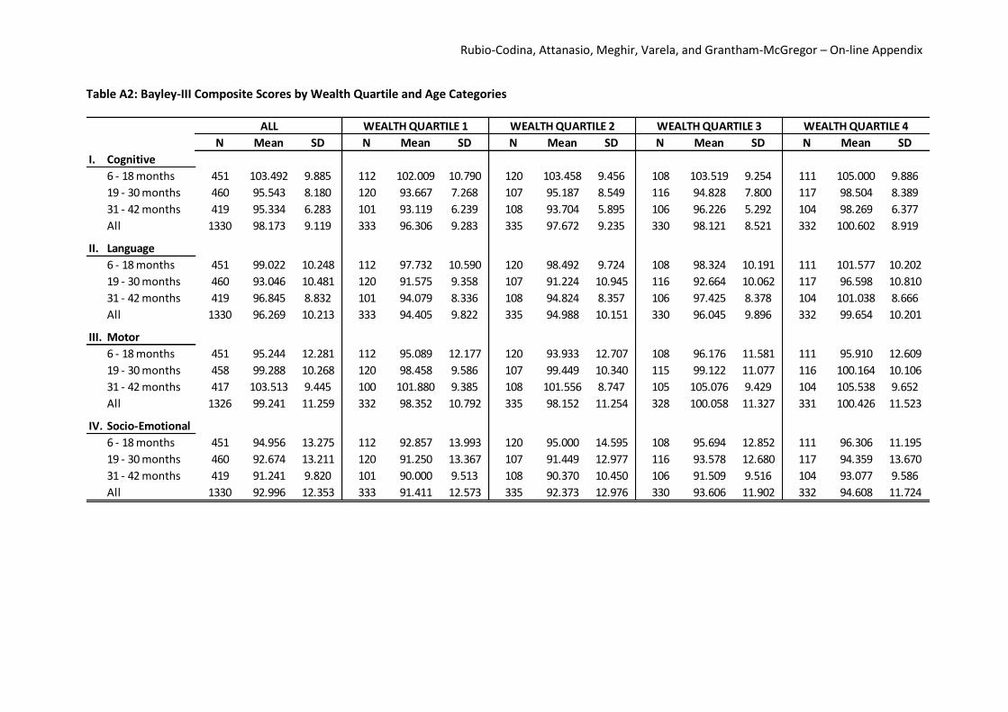
Table A2: Bayley-III Composite Scores by Wealth Quartile and Age Categories

N Mean SD N Mean SD N Mean SD N Mean SD N Mean SD

I. Cognitive

6 - 18 months 451 103.492 9.885 112 102.009 10.790 120 103.458 9.456 108 103.519 9.254 111 105.000 9.886

19 - 30 months 460 95.543 8.180 120 93.667 7.268 107 95.187 8.549 116 94.828 7.800 117 98.504 8.389

31 - 42 months 419 95.334 6.283 101 93.119 6.239 108 93.704 5.895 106 96.226 5.292 104 98.269 6.377

All 1330 98.173 9.119 333 96.306 9.283 335 97.672 9.235 330 98.121 8.521 332 100.602 8.919

II. Language

6 - 18 months 451 99.022 10.248 112 97.732 10.590 120 98.492 9.724 108 98.324 10.191 111 101.577 10.202

19 - 30 months 460 93.046 10.481 120 91.575 9.358 107 91.224 10.945 116 92.664 10.062 117 96.598 10.810

31 - 42 months 419 96.845 8.832 101 94.079 8.336 108 94.824 8.357 106 97.425 8.378 104 101.038 8.666

All 1330 96.269 10.213 333 94.405 9.822 335 94.988 10.151 330 96.045 9.896 332 99.654 10.201

III. Motor

6 - 18 months 451 95.244 12.281 112 95.089 12.177 120 93.933 12.707 108 96.176 11.581 111 95.910 12.609

19 - 30 months 458 99.288 10.268 120 98.458 9.586 107 99.449 10.340 115 99.122 11.077 116 100.164 10.106

31 - 42 months 417 103.513 9.445 100 101.880 9.385 108 101.556 8.747 105 105.076 9.429 104 105.538 9.652

All 1326 99.241 11.259 332 98.352 10.792 335 98.152 11.254 328 100.058 11.327 331 100.426 11.523

IV. Socio-Emotional

6 - 18 months 451 94.956 13.275 112 92.857 13.993 120 95.000 14.595 108 95.694 12.852 111 96.306 11.195

19 - 30 months 460 92.674 13.211 120 91.250 13.367 107 91.449 12.977 116 93.578 12.680 117 94.359 13.670

31 - 42 months 419 91.241 9.820 101 90.000 9.513 108 90.370 10.450 106 91.509 9.516 104 93.077 9.586

All 1330 92.996 12.353 333 91.411 12.573 335 92.373 12.976 330 93.606 11.902 332 94.608 11.724

ALL WEALTH QUARTILE 1 WEALTH QUARTILE 2 WEALTH QUARTILE 3 WEALTH QUARTILE 4


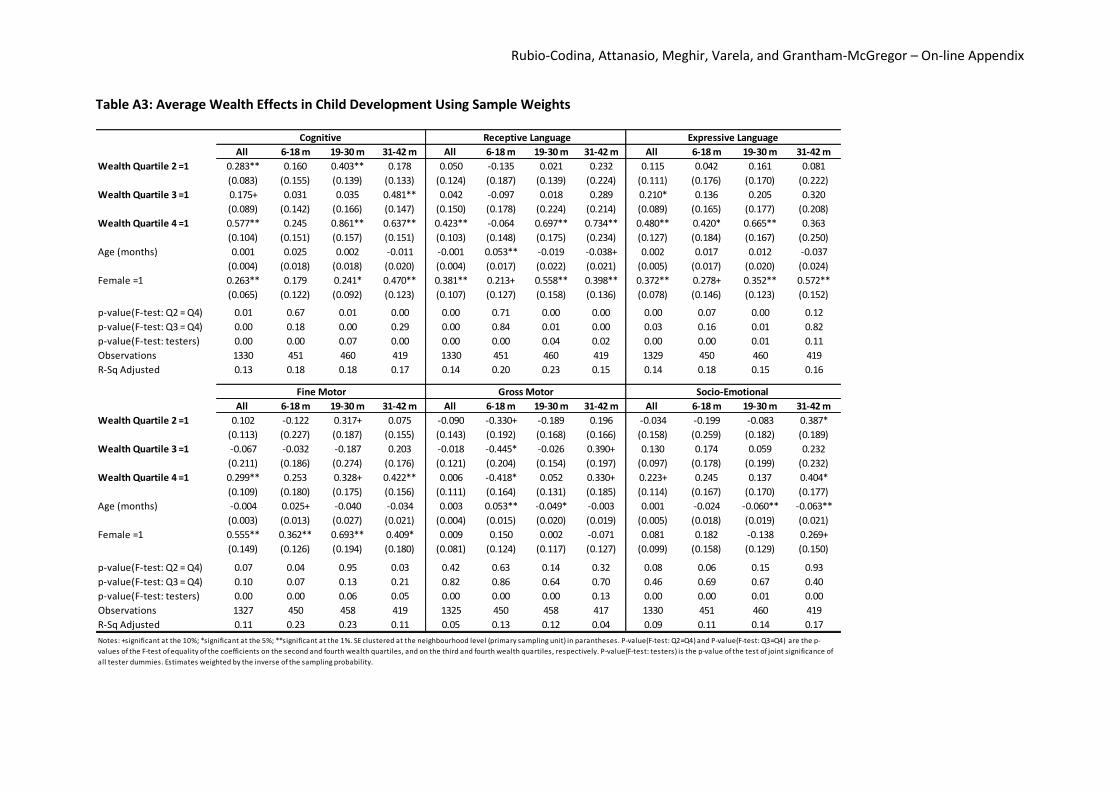
Table A3: Average Wealth Effects in Child Development Using Sample Weights

All 6-18 m 19-30 m 31-42 m All 6-18 m 19-30 m 31-42 m All 6-18 m 19-30 m 31-42 m

Wealth Quartile 2 =1 0.283** 0.160 0.403** 0.178 0.050 -0.135 0.021 0.232 0.115 0.042 0.161 0.081

(0.083) (0.155) (0.139) (0.133) (0.124) (0.187) (0.139) (0.224) (0.111) (0.176) (0.170) (0.222)

Wealth Quartile 3 =1 0.175+ 0.031 0.035 0.481** 0.042 -0.097 0.018 0.289 0.210* 0.136 0.205 0.320

(0.089) (0.142) (0.166) (0.147) (0.150) (0.178) (0.224) (0.214) (0.089) (0.165) (0.177) (0.208)

Wealth Quartile 4 =1 0.577** 0.245 0.861** 0.637** 0.423** -0.064 0.697** 0.734** 0.480** 0.420* 0.665** 0.363

(0.104) (0.151) (0.157) (0.151) (0.103) (0.148) (0.175) (0.234) (0.127) (0.184) (0.167) (0.250)

Age (months) 0.001 0.025 0.002 -0.011 -0.001 0.053** -0.019 -0.038+ 0.002 0.017 0.012 -0.037

(0.004) (0.018) (0.018) (0.020) (0.004) (0.017) (0.022) (0.021) (0.005) (0.017) (0.020) (0.024)

Female =1 0.263** 0.179 0.241* 0.470** 0.381** 0.213+ 0.558** 0.398** 0.372** 0.278+ 0.352** 0.572**

(0.065) (0.122) (0.092) (0.123) (0.107) (0.127) (0.158) (0.136) (0.078) (0.146) (0.123) (0.152)

p-value(F-test: Q2 = Q4) 0.01 0.67 0.01 0.00 0.00 0.71 0.00 0.00 0.00 0.07 0.00 0.12

p-value(F-test: Q3 = Q4) 0.00 0.18 0.00 0.29 0.00 0.84 0.01 0.00 0.03 0.16 0.01 0.82

p-value(F-test: testers) 0.00 0.00 0.07 0.00 0.00 0.00 0.04 0.02 0.00 0.00 0.01 0.11

Observations 1330 451 460 419 1330 451 460 419 1329 450 460 419

R-Sq Adjusted 0.13 0.18 0.18 0.17 0.14 0.20 0.23 0.15 0.14 0.18 0.15 0.16


Wealth Quartile 2 =1 0.102 -0.122 0.317+ 0.075 -0.090 -0.330+ -0.189 0.196 -0.034 -0.199 -0.083 0.387*

(0.113) (0.227) (0.187) (0.155) (0.143) (0.192) (0.168) (0.166) (0.158) (0.259) (0.182) (0.189)

Wealth Quartile 3 =1 -0.067 -0.032 -0.187 0.203 -0.018 -0.445* -0.026 0.390+ 0.130 0.174 0.059 0.232

(0.211) (0.186) (0.274) (0.176) (0.121) (0.204) (0.154) (0.197) (0.097) (0.178) (0.199) (0.232)

Wealth Quartile 4 =1 0.299** 0.253 0.328+ 0.422** 0.006 -0.418* 0.052 0.330+ 0.223+ 0.245 0.137 0.404*

(0.109) (0.180) (0.175) (0.156) (0.111) (0.164) (0.131) (0.185) (0.114) (0.167) (0.170) (0.177)

Age (months) -0.004 0.025+ -0.040 -0.034 0.003 0.053** -0.049* -0.003 0.001 -0.024 -0.060** -0.063**

(0.003) (0.013) (0.027) (0.021) (0.004) (0.015) (0.020) (0.019) (0.005) (0.018) (0.019) (0.021)

Female =1 0.555** 0.362** 0.693** 0.409* 0.009 0.150 0.002 -0.071 0.081 0.182 -0.138 0.269+

(0.149) (0.126) (0.194) (0.180) (0.081) (0.124) (0.117) (0.127) (0.099) (0.158) (0.129) (0.150)

p-value(F-test: Q2 = Q4) 0.07 0.04 0.95 0.03 0.42 0.63 0.14 0.32 0.08 0.06 0.15 0.93

p-value(F-test: Q3 = Q4) 0.10 0.07 0.13 0.21 0.82 0.86 0.64 0.70 0.46 0.69 0.67 0.40


Observations 1327 450 458 419 1325 450 458 417 1330 451 460 419

R-Sq Adjusted 0.11 0.23 0.23 0.11 0.05 0.13 0.12 0.04 0.09 0.11 0.14 0.17

Notes: +significant at the 10%; *significant at the 5%; **significant at the 1%. SE clustered at the neighbourhood level (primary sampling unit) in parantheses. P-value(F-test: Q2=Q4) and P-value(F-test: Q3=Q4) are the p-

values of the F-test of equality of the coefficients on the second and fourth wealth quartiles, and on the third and fourth wealth quartiles, respectively. P-value(F-test: testers) is the p-value of the test of joint significance of

all tester dummies. Estimates weighted by the inverse of the sampling probability.

Cognitive Receptive Language Expressive Language

Fine Motor Gross Motor Socio-Emotional


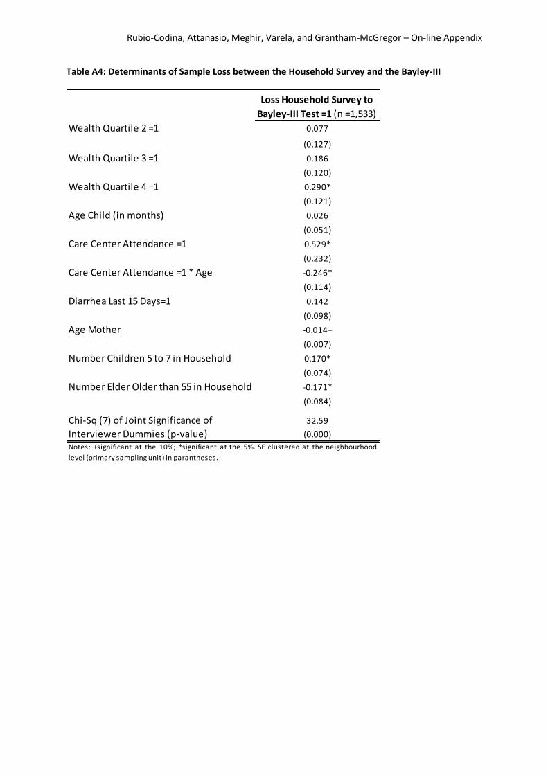
Table A4: Determinants of Sample Loss between the Household Survey and the Bayley-III

Loss Household Survey to

Bayley-III Test =1 (n =1,533)

Wealth Quartile 2 =1 0.077

(0.127)

Wealth Quartile 3 =1 0.186

(0.120)

Wealth Quartile 4 =1 0.290*

(0.121)

Age Child (in months) 0.026

(0.051)

Care Center Attendance =1 0.529*

(0.232)

Care Center Attendance =1 * Age -0.246*

(0.114)

Diarrhea Last 15 Days=1 0.142

(0.098)

Age Mother -0.014+

(0.007)

Number Children 5 to 7 in Household 0.170*

(0.074)

Number Elder Older than 55 in Household -0.171*

(0.084)

Chi-Sq (7) of Joint Significance of 32.59

Interviewer Dummies (p-value) (0.000)

Notes: +significant at the 10%; *significant at the 5%. SE clustered at the neighbourhood

level (primary sampling unit) in parantheses.


Table A5: Average Wealth Effects in Child Development Controlling for the Determinants of Sample Loss between the Household Survey and the Bayley-

III Test


Wealth Quartile 2 =1 0.209** 0.152 0.232 0.226* 0.066 0.095 -0.063 0.152 0.093 0.045 0.117 0.164

(0.077) (0.129) (0.155) (0.110) (0.058) (0.122) (0.117) (0.123) (0.078) (0.123) (0.131) (0.130)

Wealth Quartile 3 =1 0.292** 0.168 0.180 0.530** 0.140* 0.080 0.046 0.298* 0.174** 0.119 0.089 0.354**

(0.074) (0.146) (0.125) (0.116) (0.066) (0.150) (0.121) (0.125) (0.065) (0.143) (0.127) (0.124)

Wealth Quartile 4 =1 0.523** 0.269+ 0.532** 0.764** 0.390** 0.201 0.262* 0.763** 0.502** 0.476** 0.414** 0.661**

(0.078) (0.137) (0.117) (0.129) (0.067) (0.122) (0.127) (0.134) (0.074) (0.147) (0.125) (0.124)

Age (months) -0.010 0.016 -0.008 -0.018 -0.017* -0.006 -0.034 -0.023 -0.002 -0.014 -0.026 -0.006

(0.009) (0.027) (0.025) (0.030) (0.008) (0.022) (0.022) (0.031) (0.009) (0.028) (0.023) (0.027)

Female =1 0.180** 0.240* 0.149+ 0.210* 0.175** 0.118 0.294** 0.162 0.309** 0.209* 0.378** 0.370**

(0.053) (0.100) (0.089) (0.087) (0.055) (0.089) (0.085) (0.101) (0.056) (0.097) (0.090) (0.104)

p-value(F-test: Q2 = Q4) 0.00 0.36 0.05 0.00 0.00 0.41 0.02 0.00 0.00 0.01 0.03 0.00

p-value(F-test: Q3 = Q4) 0.00 0.49 0.00 0.04 0.00 0.37 0.05 0.00 0.00 0.07 0.01 0.02


Observations 1330 451 460 419 1330 451 460 419 1329 450 460 419

R-Sq Adjusted 0.12 0.09 0.11 0.20 0.13 0.24 0.11 0.12 0.11 0.12 0.09 0.13


Wealth Quartile 2 =1 0.106 0.119 0.141 0.014 -0.054 -0.223+ 0.038 0.025 0.093 0.111 0.153 0.032

(0.075) (0.130) (0.142) (0.139) (0.076) (0.130) (0.124) (0.142) (0.077) (0.130) (0.144) (0.160)

Wealth Quartile 3 =1 0.174* 0.165 0.059 0.274* 0.013 -0.191 0.003 0.276* 0.194* 0.257+ 0.188 0.188

(0.067) (0.121) (0.122) (0.128) (0.079) (0.151) (0.137) (0.122) (0.076) (0.142) (0.115) (0.137)

Wealth Quartile 4 =1 0.266** 0.226+ 0.225+ 0.352* -0.018 -0.202 0.002 0.146 0.295** 0.292* 0.204+ 0.382**

(0.077) (0.120) (0.122) (0.148) (0.089) (0.152) (0.118) (0.157) (0.079) (0.133) (0.121) (0.141)

Age (months) -0.012 -0.033 -0.011 0.019 0.002 -0.001 -0.025 0.049+ 0.034** 0.059** -0.150** 0.046

(0.009) (0.030) (0.027) (0.026) (0.008) (0.026) (0.024) (0.029) (0.010) (0.022) (0.027) (0.032)

Female =1 0.290** 0.336** 0.317** 0.220* -0.028 -0.110 0.090 -0.051 0.124* 0.100 0.043 0.241*

(0.054) (0.101) (0.081) (0.101) (0.045) (0.090) (0.090) (0.089) (0.054) (0.089) (0.081) (0.094)

p-value(F-test: Q2 = Q4) 0.05 0.38 0.55 0.04 0.70 0.88 0.77 0.45 0.02 0.13 0.67 0.05

p-value(F-test: Q3 = Q4) 0.23 0.64 0.16 0.59 0.69 0.94 0.99 0.34 0.19 0.80 0.88 0.12


Observations 1327 450 458 419 1325 450 458 417 1330 451 460 419

R-Sq Adjusted 0.09 0.13 0.09 0.09 0.05 0.02 0.11 0.09 0.09 0.09 0.16 0.11



all tester dummies. All regressions include the following controls (significant determinants of attrition as shown in Table A4): age of the mother, number of children 5-7 living in the household, number of elders (older than

65) living in the household, attendance to child care center, attendance to child care center interacted with age.




Table A6: Average Wealth Effects in Child Development Correcting for Selection into the Bayley-III Test (Heckman Correction)


Wealth Quartile 2 =1 0.197* 0.095 0.252+ 0.286* 0.076 0.094 0.006 0.107 0.099 -0.009 0.146 0.218

(0.083) (0.139) (0.152) (0.117) (0.059) (0.118) (0.115) (0.124) (0.081) (0.135) (0.127) (0.138)

Wealth Quartile 3 =1 0.287** 0.113 0.181 0.644** 0.163* 0.089 0.096 0.278* 0.184** 0.062 0.119 0.462**

(0.077) (0.146) (0.117) (0.126) (0.066) (0.140) (0.116) (0.134) (0.065) (0.140) (0.121) (0.142)

Wealth Quartile 4 =1 0.531** 0.285* 0.534** 0.883** 0.428** 0.215+ 0.340** 0.765** 0.516** 0.460** 0.444** 0.731**

(0.078) (0.131) (0.118) (0.129) (0.065) (0.119) (0.124) (0.124) (0.074) (0.141) (0.120) (0.142)

Age (months) -0.002 -0.002 0.011 0.001 0.001 0.007 0.003 0.000 0.000 -0.015 -0.012 -0.030*

(0.003) (0.012) (0.015) (0.014) (0.003) (0.011) (0.015) (0.013) (0.003) (0.012) (0.013) (0.015)

Female =1 0.172** 0.177+ 0.153+ 0.305** 0.179** 0.103 0.302** 0.169+ 0.316** 0.184+ 0.369** 0.450**

(0.053) (0.101) (0.085) (0.096) (0.055) (0.087) (0.085) (0.097) (0.056) (0.096) (0.095) (0.106)

p-value(F-test: Q2 = Q4) 0.00 0.00 0.00 0.00 0.00 0.00 0.00 0.01 0.00 0.00 0.00 0.12

p-value(F-test: Q3 = Q4) 0.00 0.16 0.05 0.00 0.00 0.32 0.01 0.00 0.00 0.00 0.01 0.00


p-value(Wald Test Indep) 0.09 0.00 0.58 0.00 0.89 0.86 0.70 0.66 0.97 0.23 0.32 0.00

Observations 1533 531 533 469 1533 531 533 469 1533 531 533 469


Wealth Quartile 2 =1 0.123 0.123 0.056 0.051 -0.093 0.006 0.032 0.052 0.103 0.014 0.134 0.038

(0.081) (0.129) (0.149) (0.151) (0.081) (0.016) (0.117) (0.143) (0.075) (0.154) (0.136) (0.158)

Wealth Quartile 3 =1 0.173* 0.191 -0.083 0.311* -0.021 -0.316* -0.058 0.357* 0.184* 0.151 0.141 0.188

(0.068) (0.117) (0.125) (0.138) (0.083) (0.141) (0.133) (0.139) (0.075) (0.148) (0.115) (0.135)

Wealth Quartile 4 =1 0.259** 0.230* 0.095 0.384** -0.058 -0.255+ -0.011 0.221 0.274** 0.264+ 0.190 0.401**

(0.078) (0.115) (0.121) (0.144) (0.082) (0.138) (0.107) (0.164) (0.075) (0.148) (0.126) (0.128)

Age (month) 0.001 0.003 -0.005 -0.007 -0.002 -0.272* 0.008 -0.016 0.002 -0.023+ -0.043** -0.024

(0.003) (0.010) (0.016) (0.017) (0.003) (0.135) (0.014) (0.016) (0.002) (0.013) (0.012) (0.015)

Female =1 0.308** 0.341** 0.307** 0.226* -0.046 -0.166+ 0.073 0.053 0.130* 0.065 0.061 0.220*

(0.054) (0.102) (0.092) (0.101) (0.048) (0.099) (0.086) (0.106) (0.053) (0.100) (0.080) (0.099)

p-value(F-test: Q2 = Q4) 0.00 0.00 0.00 0.01 0.00 0.00 0.00 0.00 0.00 0.00 0.00 0.00

p-value(F-test: Q3 = Q4) 0.10 0.38 0.79 0.03 0.71 0.77 0.70 0.28 0.04 0.08 0.66 0.03


p-value(Wald Test Indep) 0.08 0.50 0.00 0.79 0.00 0.00 0.05 0.00 0.23 0.00 0.28 0.17

Observations 1533 531 533 469 1533 531 533 469 1533 531 533 469Notes: +significant at the 10%; *significant at the 5%; **significant at the 1%. SE clustered at the neighbourhood level (primary sampling unit) in parantheses. Second stage of Heckman selection correction model reported,

where first stage includes the identity of the interviewer as the ommitted explanatory variable. p-value for the Wald Test of Independence (rho =0) reported. P-value(F-test: Q2=Q4) and P-value(F-test: Q3=Q4) are the p-


all tester dummies.




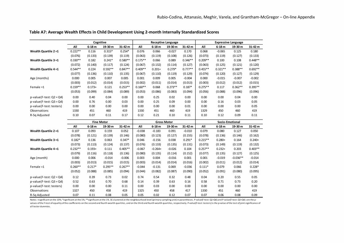
Table A7: Average Wealth Effects in Child Development Using 2-month Internally Standardized Scores


Wealth Quartile 2 =1 0.222** 0.116 0.315* 0.254* 0.076 0.066 -0.027 0.170 0.068 -0.065 0.125 0.180

(0.076) (0.133) (0.139) (0.119) (0.063) (0.119) (0.108) (0.126) (0.073) (0.119) (0.127) (0.133)

Wealth Quartile 3 =1 0.330** 0.182 0.241* 0.580** 0.175** 0.066 0.089 0.346** 0.209** 0.100 0.108 0.448**

(0.072) (0.140) (0.117) (0.124) (0.067) (0.132) (0.114) (0.127) (0.063) (0.125) (0.121) (0.120)

Wealth Quartile 4 =1 0.544** 0.224 0.592** 0.847** 0.409** 0.201+ 0.279* 0.777** 0.455** 0.321** 0.388** 0.692**

(0.077) (0.136) (0.110) (0.135) (0.067) (0.110) (0.119) (0.129) (0.074) (0.120) (0.127) (0.129)

Age (months) 0.000 0.005 0.007 0.005 0.001 0.009 0.005 -0.004 0.000 -0.015 -0.007 -0.002

(0.003) (0.012) (0.014) (0.015) (0.002) (0.011) (0.014) (0.013) (0.003) (0.012) (0.012) (0.015)

Female =1 0.159** 0.173+ 0.121 0.253** 0.160** 0.068 0.273** 0.187* 0.275** 0.117 0.362** 0.395**

(0.053) (0.099) (0.084) (0.089) (0.053) (0.086) (0.083) (0.094) (0.056) (0.088) (0.096) (0.096)

p-value(F-test: Q2 = Q4) 0.00 0.40 0.04 0.00 0.00 0.25 0.02 0.00 0.00 0.00 0.04 0.00

p-value(F-test: Q3 = Q4) 0.00 0.76 0.00 0.03 0.00 0.25 0.09 0.00 0.00 0.16 0.03 0.05


Observations 1330 451 460 419 1330 451 460 419 1329 450 460 419

R-Sq Adjusted 0.10 0.07 0.11 0.17 0.12 0.21 0.10 0.11 0.10 0.12 0.09 0.11


Wealth Quartile 2 =1 0.107 0.093 0.159 0.052 -0.038 -0.183 0.091 -0.010 0.079 0.080 0.127 0.050

(0.078) (0.121) (0.139) (0.146) (0.080) (0.123) (0.127) (0.155) (0.078) (0.136) (0.146) (0.162)

Wealth Quartile 3 =1 0.182* 0.136 0.063 0.347* 0.046 -0.156 0.038 0.291* 0.215** 0.280+ 0.164 0.240+

(0.073) (0.113) (0.124) (0.137) (0.076) (0.133) (0.135) (0.131) (0.073) (0.149) (0.119) (0.132)

Wealth Quartile 4 =1 0.232** 0.193+ 0.111 0.405** -0.067 -0.264+ -0.026 0.104 0.257** 0.232+ 0.203 0.403**

(0.079) (0.116) (0.118) (0.136) (0.080) (0.135) (0.114) (0.152) (0.077) (0.135) (0.127) (0.125)

Age (month) 0.000 0.006 -0.014 -0.006 0.003 0.004 -0.016 0.001 0.001 -0.019 -0.036** -0.014

(0.003) (0.013) (0.015) (0.015) (0.003) (0.014) (0.014) (0.016) (0.002) (0.011) (0.012) (0.014)

Female =1 0.260** 0.217* 0.295** 0.267** -0.044 -0.131 0.069 -0.036 0.111* 0.079 0.066 0.228*

(0.052) (0.088) (0.085) (0.094) (0.044) (0.082) (0.087) (0.090) (0.052) (0.091) (0.080) (0.095)

p-value(F-test: Q2 = Q4) 0.12 0.39 0.73 0.02 0.74 0.54 0.32 0.48 0.04 0.20 0.55 0.05

p-value(F-test: Q3 = Q4) 0.52 0.63 0.70 0.68 0.14 0.39 0.63 0.16 0.58 0.71 0.73 0.20


Observations 1327 450 458 419 1325 450 458 417 1330 451 460 419

R-Sq Adjusted 0.07 0.11 0.08 0.05 0.05 0.02 0.12 0.07 0.07 0.06 0.08 0.09



all tester dummies.




Table A8: Average Wealth Effects in Child Development Using Composite Scores

All 6-18 m 19-30 m 31-42 m All 6-18 m 19-30 m 31-42 m All 6-18 m 19-30 m 31-42 m All 6-18 m 19-30 m 31-42 m

Wealth Quartile 2 =1 1.196+ 0.825 1.613 0.968 0.307 -0.165 -0.094 1.149 -0.056 -1.633 1.235 -0.089 0.935 2.037 0.367 0.653

(0.627) (1.235) (1.051) (0.713) (0.617) (1.077) (1.079) (1.090) (0.808) (1.461) (1.315) (1.362) (0.908) (1.764) (1.729) (1.466)

Wealth Quartile 3 =1 1.942** 1.022 1.122 3.193** 1.783** 0.553 1.015 3.559** 1.266+ -0.793 0.790 3.318* 1.975* 2.955 1.609 1.622

(0.610) (1.325) (0.957) (0.809) (0.596) (1.226) (1.248) (1.067) (0.753) (1.461) (1.347) (1.379) (0.902) (1.969) (1.472) (1.284)

Wealth Quartile 4 =1 4.187** 2.599* 4.425** 5.136** 4.959** 3.280** 4.419** 7.115** 1.303 -1.029 0.971 3.576* 3.188** 4.059* 3.048+ 3.045*

(0.633) (1.238) (0.962) (0.966) (0.613) (1.113) (1.285) (1.096) (0.881) (1.463) (1.315) (1.370) (0.939) (1.861) (1.698) (1.175)

Age (mth) -1.147** -0.429** -0.247* 0.096 -3.670** -1.059** 0.426** 0.142 0.900** 1.132** 0.055 0.048 -0.653** -0.431** -0.527** 0.368*

(0.097) (0.119) (0.113) (0.101) (0.449) (0.126) (0.125) (0.124) (0.127) (0.145) (0.138) (0.146) (0.184) (0.151) (0.149) (0.147)

Age Squared 0.017** 0.132** -0.011** 0.010**

(0.002) (0.020) (0.003) (0.004)

Age Cube -0.001**

(0.000)

Female =1 1.830** 2.626** 1.482* 1.500* 2.992** 1.975* 4.155** 3.210** 2.465** 1.935+ 3.252** 1.932* 1.514* 0.976 1.166 2.346*

(0.437) (0.944) (0.719) (0.573) (0.503) (0.815) (0.891) (0.910) (0.538) (1.143) (0.928) (0.954) (0.673) (1.301) (1.066) (1.024)

Mean Dep Var 98.17 103.49 95.54 95.33 96.27 99.02 93.05 96.84 99.24 95.24 99.29 103.51 93.00 94.96 92.67 91.24

SD Dep Var 9.12 9.89 8.18 6.28 10.21 10.25 10.48 8.83 11.26 12.28 10.27 9.45 12.35 13.27 13.21 9.82

Gap Q4 - Q1 (in SD) 0.46 0.26 0.54 0.82 0.49 0.32 0.42 0.81 0.12 -0.08 0.09 0.38 0.26 0.31 0.23 0.31

p-value(F-test: Q2 = Q4) 0.00 0.13 0.01 0.00 0.00 0.00 0.00 0.00 0.12 0.70 0.84 0.01 0.01 0.22 0.08 0.15

p-value(F-test: Q3 = Q4) 0.00 0.23 0.00 0.02 0.00 0.03 0.01 0.00 0.97 0.88 0.90 0.85 0.18 0.53 0.36 0.29

p-value(F-test: testers) 0.00 0.00 0.00 0.00 0.00 0.00 0.00 0.10 0.00 0.00 0.00 0.03 0.00 0.00 0.00 0.00

Observations 1330 451 460 419 1330 451 460 419 1326 451 458 417 1330 451 460 419

R-Sq Adjusted 0.26 0.11 0.12 0.16 0.24 0.35 0.15 0.13 0.18 0.16 0.12 0.05 0.09 0.06 0.11 0.08

Cognitive Language Motor Socio-Emotional

Notes: +significant at the 10%; *significant at the 5%; **significant at the 1%. SE clustered at the neighbourhood level (primary sampling unit) in parantheses. Gap Q4 - Q1 is the size of the SES gap between the fourth and first quartile. It is

computed by diving the estimated coefficient on wealth quartile 4 by the standard deviation (SD) of the estimation sample. P-value(F-test: Q2=Q4) and P-value(F-test: Q3=Q4) are the p-values of the F-test of equality of the coefficients on the

second and fourth wealth quartiles, and on the third and fourth wealth quartiles, respectively. P-value(F-test: testers) is the p-value of the test of joint significant of all tester dummies.


13

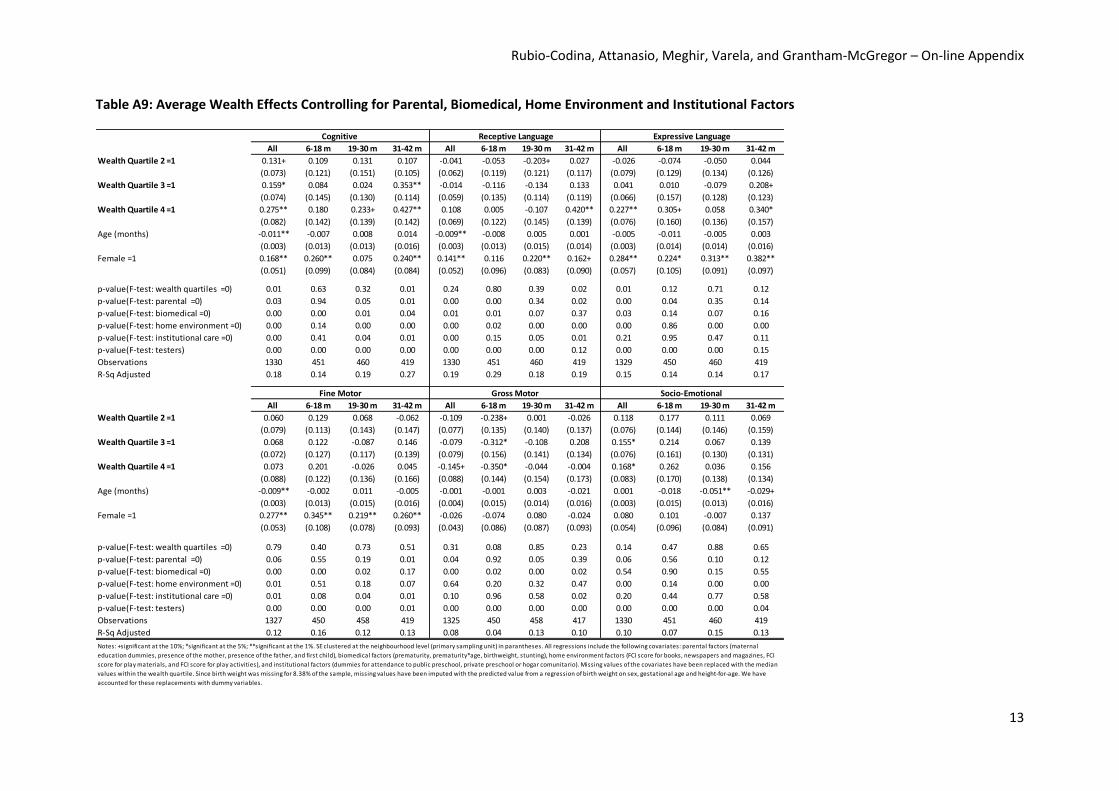
Table A9: Average Wealth Effects Controlling for Parental, Biomedical, Home Environment and Institutional Factors


Wealth Quartile 2 =1 0.131+ 0.109 0.131 0.107 -0.041 -0.053 -0.203+ 0.027 -0.026 -0.074 -0.050 0.044

(0.073) (0.121) (0.151) (0.105) (0.062) (0.119) (0.121) (0.117) (0.079) (0.129) (0.134) (0.126)

Wealth Quartile 3 =1 0.159* 0.084 0.024 0.353** -0.014 -0.116 -0.134 0.133 0.041 0.010 -0.079 0.208+

(0.074) (0.145) (0.130) (0.114) (0.059) (0.135) (0.114) (0.119) (0.066) (0.157) (0.128) (0.123)

Wealth Quartile 4 =1 0.275** 0.180 0.233+ 0.427** 0.108 0.005 -0.107 0.420** 0.227** 0.305+ 0.058 0.340*

(0.082) (0.142) (0.139) (0.142) (0.069) (0.122) (0.145) (0.139) (0.076) (0.160) (0.136) (0.157)

Age (months) -0.011** -0.007 0.008 0.014 -0.009** -0.008 0.005 0.001 -0.005 -0.011 -0.005 0.003

(0.003) (0.013) (0.013) (0.016) (0.003) (0.013) (0.015) (0.014) (0.003) (0.014) (0.014) (0.016)

Female =1 0.168** 0.260** 0.075 0.240** 0.141** 0.116 0.220** 0.162+ 0.284** 0.224* 0.313** 0.382**

(0.051) (0.099) (0.084) (0.084) (0.052) (0.096) (0.083) (0.090) (0.057) (0.105) (0.091) (0.097)

p-value(F-test: wealth quartiles =0) 0.01 0.63 0.32 0.01 0.24 0.80 0.39 0.02 0.01 0.12 0.71 0.12

p-value(F-test: parental =0) 0.03 0.94 0.05 0.01 0.00 0.00 0.34 0.02 0.00 0.04 0.35 0.14

p-value(F-test: biomedical =0) 0.00 0.00 0.01 0.04 0.01 0.01 0.07 0.37 0.03 0.14 0.07 0.16

p-value(F-test: home environment =0) 0.00 0.14 0.00 0.00 0.00 0.02 0.00 0.00 0.00 0.86 0.00 0.00

p-value(F-test: institutional care =0) 0.00 0.41 0.04 0.01 0.00 0.15 0.05 0.01 0.21 0.95 0.47 0.11


Observations 1330 451 460 419 1330 451 460 419 1329 450 460 419

R-Sq Adjusted 0.18 0.14 0.19 0.27 0.19 0.29 0.18 0.19 0.15 0.14 0.14 0.17


Wealth Quartile 2 =1 0.060 0.129 0.068 -0.062 -0.109 -0.238+ 0.001 -0.026 0.118 0.177 0.111 0.069

(0.079) (0.113) (0.143) (0.147) (0.077) (0.135) (0.140) (0.137) (0.076) (0.144) (0.146) (0.159)

Wealth Quartile 3 =1 0.068 0.122 -0.087 0.146 -0.079 -0.312* -0.108 0.208 0.155* 0.214 0.067 0.139

(0.072) (0.127) (0.117) (0.139) (0.079) (0.156) (0.141) (0.134) (0.076) (0.161) (0.130) (0.131)

Wealth Quartile 4 =1 0.073 0.201 -0.026 0.045 -0.145+ -0.350* -0.044 -0.004 0.168* 0.262 0.036 0.156

(0.088) (0.122) (0.136) (0.166) (0.088) (0.144) (0.154) (0.173) (0.083) (0.170) (0.138) (0.134)

Age (months) -0.009** -0.002 0.011 -0.005 -0.001 -0.001 0.003 -0.021 0.001 -0.018 -0.051** -0.029+

(0.003) (0.013) (0.015) (0.016) (0.004) (0.015) (0.014) (0.016) (0.003) (0.015) (0.013) (0.016)

Female =1 0.277** 0.345** 0.219** 0.260** -0.026 -0.074 0.080 -0.024 0.080 0.101 -0.007 0.137

(0.053) (0.108) (0.078) (0.093) (0.043) (0.086) (0.087) (0.093) (0.054) (0.096) (0.084) (0.091)

p-value(F-test: wealth quartiles =0) 0.79 0.40 0.73 0.51 0.31 0.08 0.85 0.23 0.14 0.47 0.88 0.65

p-value(F-test: parental =0) 0.06 0.55 0.19 0.01 0.04 0.92 0.05 0.39 0.06 0.56 0.10 0.12

p-value(F-test: biomedical =0) 0.00 0.00 0.02 0.17 0.00 0.02 0.00 0.02 0.54 0.90 0.15 0.55

p-value(F-test: home environment =0) 0.01 0.51 0.18 0.07 0.64 0.20 0.32 0.47 0.00 0.14 0.00 0.00

p-value(F-test: institutional care =0) 0.01 0.08 0.04 0.01 0.10 0.96 0.58 0.02 0.20 0.44 0.77 0.58


Observations 1327 450 458 419 1325 450 458 417 1330 451 460 419

R-Sq Adjusted 0.12 0.16 0.12 0.13 0.08 0.04 0.13 0.10 0.10 0.07 0.15 0.13

Notes: +significant at the 10%; *significant at the 5%; **significant at the 1%. SE clustered at the neighbourhood level (primary sampling unit) in parantheses. All regressions include the following covariates: parental factors (maternal

education dummies, presence of the mother, presence of the father, and first child), biomedical factors (prematurity, prematurity*age, birthweight, stunting), home environment factors (FCI score for books, newspapers and magazines, FCI

score for play materials, and FCI score for play activities), and institutional factors (dummies for attendance to public preschool, private preschool or hogar comunitario). Missing values of the covariates have been replaced with the median

values within the wealth quartile. Since birth weight was missing for 8.38% of the sample, missing values have been imputed with the predicted value from a regression of birth weight on sex, gestational age and height-for-age. We have

accounted for these replacements with dummy variables.




14

Figure A1: Spatial Distribution of Estratos in the City of Bogota

Source: http://institutodeestudiosurbanos.info/endatos/0200/02-030-vivienda/02.03.01.htm

http://institutodeestudiosurbanos.info/endatos/0200/02-030-vivienda/02.03.01.htm

the socio-economic gradient of child development: cross ... · rubio-codina, attanasio, meghir,...

Documents