the second law of nonequilibrium thermodynamics - personal pages

THE SECOND LAW OF NONEQUILIBRIUM

THERMODYNAMICS: HOW FAST TIME FLIES

PHIL ATTARD

School of Chemistry F11, University of Sydney, NSW 2006 Australia

CONTENTS

I. Introduction

A. Review and Preview

II. Linear Thermodynamics

A. Formalities

B. Quadratic Expansion

C. Time Scaling

1. Optimum Point

D. Regression Theorem

1. Asymmetry of the Transport Matrix

E. Entropy Production

F. Reservoir

G. Intermediate Regime and Maximum Flux

III. Nonlinear Thermodynamics

A. Quadratic Expansion

B. Parity

C. Time Scaling

1. Optimum Intermediate Point

D. Linear Limit of Nonlinear Coefficients

E. Exchange with a Reservoir

F. Rate of Entropy Production

IV. Nonequilibrium Statistical Mechanics

A. Steady-State Probability Distribution

B. Relationship with Green–Kubo Theory

C. Microstate Transitions

1. Adiabatic Evolution

2. Stochastic Transition

3. Stationary Steady-State Probability

4. Forward and Reverse Transitions

Advances in Chemical Physics, Volume 140, edited by Stuart A. RiceCopyright # 2008 John Wiley & Sons, Inc.

1

COPYRIG

HTED M

ATERIAL

V. Time-Dependent Mechanical Work

A. Phase Space Probability

B. Transition Probability

VI. Nonequilibrium Quantum Statistical Mechanics

VII. Heat Flow

A. Thermodynamic Variables

B. Gaussian Approximation

C. Second Entropy

1. Isolated System

2. Reservoirs

3. Rate of Entropy Production

D. Phase Space Probability Distribution

VIII. Monte Carlo Simulations of Heat Flow

A. System Details

B. Metropolis Algorithm

C. Nonequilibrium Molecular Dynamics

D. Monte Carlo Results

1. Structure

2. Dynamics

IX. Conclusion

Acknowledgments

References

I. INTRODUCTION

The Second Law of Equilibrium Thermodynamics may be stated:

The entropy increases during spontaneous changes

in the structure of the total system ð1Þ

This is a law about the equilibrium state, when macroscopic change has ceased; it

is the state, according to the law, of maximum entropy. It is not really a law about

nonequilibrium per se, not in any quantitative sense, although the law does

introduce the notion of a nonequilibrium state constrained with respect to

structure. By implication, entropy is perfectly well defined in such a non-

equilibrium macrostate (otherwise, how could it increase?), and this constrained

entropy is less than the equilibrium entropy. Entropy itself is left undefined by the

Second Law, and it was only later that Boltzmann provided the physical inter-

pretation of entropy as the number of molecular configurations in a macrostate.

This gave birth to his probability distribution and hence to equilibrium statistical

mechanics.

The reason that the Second Law has no quantitative relevance to non-

equilibrium states is that it gives the direction of change, not the rate of change.

So although it allows the calculation of the thermodynamic force that drives the

system toward equilibrium, it does not provide a basis for calculating the all

2 phil attard

important rate at which the system evolves. A full theory for the nonequili-

brium state cannot be based solely on the Second Law or the entropy it

invokes.

This begs the question of whether a comparable law exists for nonequilibrium

systems. This chapter presents a theory for nonequilibrium thermodynamics and

statistical mechanics based on such a law written in a form analogous to the

equilibrium version:

The second entropy increases during spontaneous changes

in the dynamic structure of the total systemð2Þ

Here dynamic structure gives a macroscopic flux or rate; it is a transition between

macrostates in a specified time. The law invokes the notion of constrained fluxes

and the notion that fluxes cease to change in the optimum state, which, in

common parlance, is the steady state. In other words, the principle governing

nonequilibrium systems is that in the transient regime fluxes develop and evolve

to increase the second entropy, and that in the steady state the macroscopic fluxes

no longer change and the second entropy is maximal. The second entropy could

also be called the transition entropy, and as the reader has probably already

guessed, it is the number of molecular configurations associated with a transition

between macrostates in a specified time.

This nonequilibrium Second Law provides a basis for a theory for

nonequilibrium thermodynamics. The physical identification of the second

entropy in terms of molecular configurations allows the development of the

nonequilibrium probability distribution, which in turn is the centerpiece for

nonequilibrium statistical mechanics. The two theories span the very large and

the very small. The aim of this chapter is to present a coherent and self-

contained account of these theories, which have been developed by the author

and presented in a series of papers [1–7]. The theory up to the fifth paper has

been reviewed previously [8], and the present chapter consolidates some of this

material and adds the more recent developments.

Because the focus is on a single, albeit rather general, theory, only a limited

historical review of the nonequilibrium field is given (see Section IA). That is

not to say that other work is not mentioned in context in other parts of this

chapter. An effort has been made to identify where results of the present theory

have been obtained by others, and in these cases some discussion of the

similarities and differences is made, using the nomenclature and perspective of

the present author. In particular, the notion and notation of constraints and

exchange with a reservoir that form the basis of the author’s approach to

equilibrium thermodynamics and statistical mechanics [9] are used as well for

the present nonequilibrium theory.

the second law of nonequilibrium thermodynamics 3

A. Review and Preview

The present theory can be placed in some sort of perspective by dividing the

nonequilibrium field into thermodynamics and statistical mechanics. As will

become clearer later, the division between the two is fuzzy, but for the present

purposes nonequilibrium thermodynamics will be considered that phenomen-

ological theory that takes the existence of the transport coefficients and laws as

axiomatic. Nonequilibrium statistical mechanics will be taken to be that field that

deals with molecular-level (i.e., phase space) quantities such as probabilities and

time correlation functions. The probability, fluctuations, and evolution of

macrostates belong to the overlap of the two fields.

Perhaps the best starting point in a review of the nonequilibrium field, and

certainly the work that most directly influenced the present theory, is Onsager’s

celebrated 1931 paper on the reciprocal relations [10]. This showed that the

symmetry of the linear hydrodynamic transport matrix was a consequence of the

time reversibility of Hamilton’s equations of motion. This is an early example of

the overlap between macroscopic thermodynamics and microscopic statistical

mechanics. The consequences of time reversibility play an essential role in the

present nonequilibrium theory, and in various fluctuation and work theorems to

be discussed shortly.

Moving upward to the macroscopic level, the most elementary phenomen-

ological theories for nonequilibrium thermodynamics are basically hydrody-

namics plus localized equilibrium thermodynamics [11, 12]. In the so-called

soft sciences, including, as examples, biological, environmental, geological,

planetary, atmospheric, climatological, and paleontological sciences, the study

of evolution and rates of change is all important. This has necessarily stimulated

much discussion of nonequilibrium principles and approaches, which are

generally related to the phenomenological theories just described [13–18]. More

advanced phenomenological theories for nonequilibrium thermodynamics in its

own right have been pursued [19–23]. The phenomenological theories generally

assert the existence of a nonequilibrium potential that is a function of the fluxes,

and whose derivatives are consistent with the transport laws and other symmetry

requirements.

In view of the opening discussion of the two second laws of thermodynamics,

in analyzing all theories, phenomenological and otherwise, it is important to ask

two questions:

Does the theory invoke the second entropy;or only the first entropy and its rate of change? ð3Þ

and

Is the relationship being invoked true in general;or is it only true in the optimum or steady state? ð4Þ

4 phil attard

If the approach does not go beyond the ordinary entropy, or if it applies an

optimized result to a constrained state, then one can immediately conclude that a

quantitative theory for the nonequilibrium state is unlikely to emerge. Regrettably,

for phenomenological theories of the type just discussed, the answer to both

questions is usually negative. The contribution of Prigogine, in particular, will be

critically assessed from these twin perspectives (see Section IIE).

Moving downward to the molecular level, a number of lines of research

flowed from Onsager’s seminal work on the reciprocal relations. The symmetry

rule was extended to cases of mixed parity by Casimir [24], and to nonlinear

transport by Grabert et al. [25] Onsager, in his second paper [10], expressed the

linear transport coefficient as an equilibrium average of the product of the

present and future macrostates. Nowadays, this is called a time correlation

function, and the expression is called Green–Kubo theory [26–30].

The transport coefficient gives the ratio of the flux (or future macrostate

velocity) to the conjugate driving force (mechanical or thermodynamic). It

governs the dissipative force during the stochastic and driven motion of a

macrostate, and it is related to the strength of the fluctuations by the fluctuation-

dissipation theorem [31]. Onsager and Machlup [32] recognized that the transport

theory gave rise to a related stochastic differential equation for the evolution of a

macrostate that is called the Langevin equation (or the Smoluchowski equation in

the overdamped case). Applied to the evolution of a probability distribution it is

the Fokker–Planck equation [33]. In the opinion of the present author, stochastic

differential equations such as these result from a fundamental, molecular-level

nonequilibrium theory, but in themselves are not fundamental and they do not

provide a basis for constructing a full nonequilibrium theory.

Onsager and Machlup [32] gave expressions for the probability of a path of

macrostates and, in particular, for the probability of a transition between two

macrostates. The former may be regarded as the solution of a stochastic

differential equation. It is technically a Gaussian Markov process, also known as

an Ornstein–Uhlenbeck process. More general stochastic processes include, for

example, the effects of spatial curvature and nonlinear transport [33–35]. These

have been accounted for by generalizing the Onsager–Machlup functional to

give the so-called thermodynamic Lagrangian [35–42]. Other thermodynamic

Lagrangians have been given [43–46]. The minimization of this functional gives

the most probable evolution in time of the macrostate, and hence one might

expect the thermodynamic Lagrangian to be related (by a minus sign) to the

second entropy that is the basis of the present theory. However, the Onsager–

Machlup functional [32] (and those generalizations of it) [35–42] fails both

questions posed above: (1) it invokes solely the rate of production of first

entropy, and (2) both expressions that it invokes for this are only valid in the

steady state, not in the constrained states that are the subject of the optimization

procedure (see Section IIE). The Onsager–Machlup functional (in two-state


transition form) is tested against computer simulation data for the thermal

conductivity time correlation function in Fig. 8.

On a related point, there have been other variational principles enunciated as a

basis for nonequilibrium thermodynamics. Hashitsume [47], Gyarmati [48, 49],

and Bochkov and Kuzovlev [50] all assert that in the steady state the rate of first

entropy production is an extremum, and all invoke a function identical to that

underlying the Onsager–Machlup functional [32]. As mentioned earlier,

Prigogine [11] (and workers in the broader sciences) [13–18] variously asserts

that the rate of first entropy production is a maximum or a minimum and invokes

the same two functions for the optimum rate of first entropy production that were

used by Onsager and Machlup [32] (see Section IIE).

Evans and Baranyai [51, 52] have explored what they describe as a nonlinear

generalization of Prigogine’s principle of minimum entropy production. In their

theory the rate of (first) entropy production is equated to the rate of phase space

compression. Since phase space is incompressible under Hamilton’s equations

of motion, which all real systems obey, the compression of phase space that

occurs in nonequilibrium molecular dynamics (NEMD) simulations is purely an

artifact of the non-Hamiltonian equations of motion that arise in implementing

the Evans–Hoover thermostat [53, 54]. (See Section VIIIC for a critical

discussion of the NEMD method.) While the NEMD method is a valid

simulation approach in the linear regime, the phase space compression induced

by the thermostat awaits physical interpretation; even if it does turn out to be

related to the rate of first entropy production, then the hurdle posed by Question

(3) remains to be surmounted.

In recent years there has been an awakening of interest in fundamental

molecular-level theorems in nonequilibrium statistical mechanics. This spurt of

theoretical and experimental activity was kindled by the work theorem

published by Jarzynski in 1997 [55]. The work theorem is in fact a trivial

consequence of the fluctuation theorem published by Evans, Cohen, and

Morriss in 1993, [56, 57] and both theorems were explicitly given earlier by

Bochkov and Kuzovlev in 1977 [58–60]. As mentioned earlier, since Onsager’s

work in 1931 [10], time reversibility has played an essential role in

nonequilibrium theory. Bochkov and Kuzovlev [60], and subsequent authors

including the present one [4], have found it exceedingly fruitful to consider the

ratio of the probability of a forward trajectory to that of the reversed trajectory.

Using time reversibility, this ratio can be related to the first entropy produced

on the forward trajectory, and it has come to be called the fluctuation theorem

[56, 57]. An alternative derivation assuming Markovian behavior of the

macrostate path probability has been given [61, 62], and it has been demon-

strated experimentally [63]. From this ratio one can show that the average of

the exponential of the negative of the entropy produced (minus work divided

by temperature) equals the exponential of the difference in initial and final

6 phil attard

Helmholtz free energies divided by temperature, which is the work theorem

[55]. For a cyclic process, the latter difference is zero, and hence the average is

unity, as shown by Bochkov and Kuzovlev [58–60]. The work theorem has been

rederived in different fashions [57, 64, 65] and verified experimentally [66].

What is remarkable about the work theorem is that it holds for arbitrary rates of

nonequilibrium work, and there is little restriction beyond the assumption of

equilibration at the beginning and end of the work and sufficiently long time

interval to neglect end effects. (See Sections IVC4 and VB for details and

generalizations.)

With the exception of the present theory, derivations of the fluctuation and

work theorems are generally for a system that is isolated during the performance

of the work (adiabatic trajectories), and the effects of a thermal or other

reservoir on the true nonequilibrium probability distribution or transition

probability are neglected. The existence and form for the nonequilibrium

probability distribution, both in the steady state and more generally, may be said

to be the holy grail of nonequilibrium statistical mechanics. The Boltzmann

distribution is the summit of the equilibrium field [67], and so there have been

many attempts to formulate its analogue in a nonequilibrium context. The most

well known is the Yamada–Kawasaki distribution [68, 69]. It must be stressed

that this distribution is an adiabatic distribution, which is to say that it assumes

that the system was in thermal equilibrium in the past, and that it was

subsequently isolated from the thermal reservoirs while the work was being

performed so that no heat was exchanged during the time-dependent process.

This is obviously a very restrictive assumption. Attempts have been made to

formulate a thermostatted form of the Yamada–Kawasaki distribution, but this

has been found to be computationally intractable [53, 70, 71]. As pointed out

earlier, most derivations of the fluctuation and work theorems are predicated on

the adiabatic assumption, and a number of authors invoke or derive the

Yamada–Kawasaki distribution, apparently unaware of its prior publication and

of its restricted applicability.

An alternative approximation to the adiabatic probability is to invoke an

instantaneous equilibrium-like probability. In the context of the work theorem,

Hatano and Sasa [72] analyzed a nonequilibrium probability distribution that

had no memory, and others have also invoked a nonequilibrium probability

distribution that is essentially a Boltzmann factor of the instantaneous value of

the time-dependent potential [73, 74].

In Sections IVA, VA, and VI the nonequilibrium probability distribution is

given in phase space for steady-state thermodynamic flows, mechanical work,

and quantum systems, respectively. (The second entropy derived in Section II

gives the probability of fluctuations in macrostates, and as such it represents the

nonequilibrium analogue of thermodynamic fluctuation theory.) The present

phase space distribution differs from the Yamada–Kawasaki distribution in that


it correctly takes into account heat exchange with a reservoir during the

mechanical work or thermodynamic flux. The probability distribution is the

product of a Boltzmann-like term, which is reversible in time, and a new term,

which is odd in time, and which once more emphasizes Onsager’s [10] foresight

in identifying time reversibility as the key to nonequilibrium behavior. In

Section IVB this phase space probability is used to derive the Green–Kubo

relations, in Section VIIIB it is used to develop a nonequilibrium Monte Carlo

algorithm, and in Fig. 7 it is shown that the algorithm is computationally

feasible and that it gives a thermal conductivity in full agreement with

conventional NEMD results.

In addition to these nonequilibrium probability densities, the present theory

also gives expressions for the transition probability and for the probability of a

phase space trajectory, in both equilibrium and nonequilibrium contexts,

(Sections IVC and VB). These sections contain the derivations and general-

izations of the fluctuation and work theorems alluded to earlier. As for the

probability density, one has to be aware that some work in the literature is based

on adiabatic transitions, whereas the present approach includes the effect of heat

flow on the transition. One also has to distinguish works that deal with

macrostate transitions, from the present approach based in phase space, which

of course includes macrostate transition by integration over the microstates. The

second entropy, which is the basis for the nonequilibrium second law advocated

earlier, determines such transitions pairwise, and for an interval divided into

segments of intermediate length, it determines a macrostate path by a Markov

procedure (Sections IIC and IIIC). The phase space trajectory probability

contains an adiabatic term and a stochastic term. The latter contains in essence

half the difference between the target and initial reservoir entropies. This term

may be seen to be essentially the one that is invoked in Glauber or Kawasaki

dynamics [75–78]. This form for the conditional stochastic transition

probability satisfies detailed balance for an equilibrium Boltzmann distribution,

and it has been used successfully in hybrid equilibrium molecular dynamics

algorithms [79–81]. Using the term on its own without the adiabatic

development, as in Glauber or Kawasaki dynamics, corresponds to neglecting

the coupling inherent in the second entropy, and to losing the speed of time.

II. LINEAR THERMODYNAMICS

A. Formalities

Consider an isolated system containing N molecules, and let G � fqN ; pNg be apoint in phase space, where the ith molecule has position qi and momentum pi. In

developing the nonequilibrium theory, it will be important to discuss the

behavior of the system under time reversal. Accordingly, define the conjugate

8 phil attard

point in phase space as that point with all the velocities reversed,

Gy � fqN ; ð�pÞNg. If G2 ¼ G0ðtjG1Þ is the position of the isolated system at

time t given that it was at G1 at time t ¼ 0, then Gy1 ¼ G0ðtjGy2Þ, as follows fromthe reversibility of Hamilton’s equations of motion. One also has, by definition of

the trajectory, that G1 ¼ G0ð�tjG2Þ.Macrostates are collections of microstates [9], which is to say that they are

volumes of phase space on which certain phase functions have specified values.

The current macrostate of the system gives its structure. Examples are the

position or velocity of a Brownian particle, the moments of energy or density,

their rates of change, the progress of a chemical reaction, a reaction rate, and

so on. Let x label the macrostates of interest, and let xðGÞ be the associated

phase function. The first entropy of the macrostate is

Sð1ÞðxjEÞ ¼ kB ln

ZdG dðHðGÞ � EÞ dðxðGÞ � xÞ ð5Þ

neglecting an arbitrary constant. This is the ordinary entropy; here it is called the

first entropy, to distinguish it from the second or transition entropy that is

introduced later. Here the Hamiltonian appears, and all microstates of the

isolated system with energy E are taken to be equally likely [9]. This is the

constrained entropy, since the system is constrained to be in a particular

macrostate. By definition, the probability of the macrostate is proportional to the

exponential of the entropy,

}ðxjEÞ ¼ 1

WðEÞ exp Sð1ÞðxjEÞ=kB ð6Þ

The normalizing factor is related to the unconstrained entropy by

Sð1ÞðEÞ � kB lnWðEÞ ¼ kB ln

Zdx exp SðxjEÞ=kB

¼ kB ln

ZdG dðHðGÞ � EÞ

ð7Þ

The equilibrium state, which is denoted x, is by definition both the most

likely state, }ðxjEÞ � }ðxjEÞ, and the state of maximum constrained entropy,

Sð1ÞðxjEÞ � Sð1ÞðxjEÞ. This is the statistical mechanical justification for much of

the import of the Second Law of Equilibrium Thermodynamics. The

unconstrained entropy, as a sum of positive terms, is strictly greater than the

maximal constrained entropy, which is the largest term, Sð1ÞðEÞ > Sð1ÞðxjEÞ.However, in the thermodynamic limit when fluctuations are relatively

negligible, these may be equated with relatively little error, Sð1ÞðEÞ � Sð1ÞðxjEÞ.


The macrostates can have either even or odd parity, which refers to their

behavior under time reversal or conjugation. Let Ei ¼ �1 denote the parity of

the ith microstate, so that xiðGyÞ ¼ EixiðGÞ. (It is assumed that each state is

purely even or odd; any state of mixed parity can be written as the sum of two

states of pure parity.) Loosely speaking, variables with even parity may be

called position variables, and variables with odd parity may be called velocity

variables. One can form the diagonal matrix E, with elements Eidij, so that

xðGyÞ ¼ ExðGÞ. The parity matrix is its own inverse, E E ¼ I.

The Hamiltonian is insensitive to the direction of time,HðGÞ ¼ HðGyÞ, sinceit is a quadratic function of the molecular velocities. (Since external Lorentz or

Coriolis forces arise from currents or velocities, they automatically reverse

direction under time reversal.) Hence both G and Gy have equal weight. From

this it is easily shown that Sð1ÞðxjEÞ ¼ Sð1ÞðExjEÞ.The unconditional transition probability between macrostates in time t for

the isolated system satisfies

}ðx0 xjt;EÞ¼ �ðx0jx; t;EÞ}ðxjEÞ¼ W�1E

ZdG1 dG2 dðx0� xðG2ÞÞdðx� xðG1ÞÞ dðG2 � G0ðtjG1ÞÞ dðHðG1Þ � EÞ

¼ W�1E

ZdGy1 dG

y2 dðx0�ExðGy2ÞÞdðx�ExðGy1ÞÞ dðGy1�G0ðtjGy2ÞÞdðHðGy1Þ�EÞ

¼ }ðEx Ex0jt;EÞ ð8Þ

This uses the fact that dG ¼ dGy. For macrostates all of even parity, this says that

for an isolated system the forward transition x! x0 will be observed as

frequently as the reverse x0 ! x. This is what Onsager meant by the principle of

dynamical reversibility, which he stated as ‘‘in the end every type of motion is

just as likely to occur as its reverse’’ [10, p. 412]. Note that for velocity-type

variables, the sign is reversed for the reverse transition.

The second or transition entropy is the weight of molecular configurations

associated with a transition occurring in time t,

Sð2Þðx0; xjt;EÞ ¼ kB ln

ZdG1 dðxðG0ðtjG1ÞÞ � x0Þ dðxðG1Þ � xÞ dðHðG1Þ � EÞ

ð9Þ

up to an arbitrary constant. The unconditional transition probability for x! x0 intime t is related to the second entropy by [2, 8]

}ðx0; xjt;EÞ ¼ 1

WðEÞ exp Sð2Þðx0; xjt;EÞ=kB ð10Þ

10 phil attard

Henceforth the dependence on the energy is not shown explicitly. The second

entropy reduces to the first entropy upon integration

Sð1ÞðxÞ ¼ const:þ kB ln

Zdx0 exp Sð2Þðx0; xjtÞ=kB ð11Þ

It will prove important to impose this reduction condition on the approximate

expansions given later.

The second entropy obeys the symmetry rules

Sð2Þðx0; xjtÞ ¼ Sð2Þðx; x0j � tÞ ¼ Sð2ÞðEx; Ex0jtÞ ð12Þ

The first equality follows from time homogeneity: the probability that x0 ¼xðt þ tÞ and x ¼ xðtÞ are the same as the probability that x ¼ xðt � tÞ andx0 ¼ xðtÞ. The second equality follows from microscopic reversibility: if the

molecular velocities are reversed the system retraces its trajectory in phase space.

Again, it will prove important to impose these symmetry conditions on the

following expansions.

In the formulation of the nonequilibrium second law, Eq. (2), dynamic

structure was said to be equivalent to a rate or flux. This may be seen more

clearly from the present definition of the second entropy, since the coarse

velocity can be defined as

x� � x0 � x

tð13Þ

Maximizing the second entropy with respect to x0 for fixed x yields the most

likely terminal position xðx; tÞ � x0, and hence the most likely coarse velocity

x�ðx; tÞ. Alternatively, differentiating the most likely terminal position with

respect to t yields the most likely terminal velocity, _xðx; tÞ. So constraining the

system to be in the macrostate x0 at a time t after it was in the state x is the same

as constraining the coarse velocity.

B. Quadratic Expansion

For simplicity, it is assumed that the equilibrium value of the macrostate is zero,

x ¼ 0. This means that henceforth x measures the departure of the macrostate

from its equilibrium value. In the linear regime, (small fluctuations), the first

entropy may be expanded about its equilibrium value, and to quadratic order it is

Sð1ÞðxÞ ¼ 12S : x2 ð14Þ

a constant having been neglected. Here and throughout a colon or centered dot is

used to denote scalar multiplication, and squared or juxtaposed vectors to denote


a dyad. Hence the scalar could equally be written S : x2 � x � Sx. The

thermodynamic force is defined as

XðxÞ � qSð1ÞðxÞqx

¼ Sx ð15Þ

Evidently in the linear regime the probability is Gaussian, and the correlation

matrix is therefore given by

S�1 ¼ �hxxi0=kB ð16Þ

The parity matrix commutes with the first entropy matrix, E S ¼ S E, becausethere is no coupling between variables of opposite parity at equilibrium,

hxixji0 ¼ 0 if EiEj ¼ �1. If variables of the same parity are grouped together, the

first entropy matrix is block diagonal.

This last point may be seen more clearly by defining a time-correlation

matrix related to the inverse of this,

QðtÞ � k�1B hxðt þ tÞxðtÞi0 ð17Þ

From the time-reversible nature of the equations of motion, Eq. (12), it is readily

shown that the matrix is ‘‘block-asymmetric’’:

QðtÞ ¼ EQðtÞTE ¼ EQð�tÞE ð18Þ

Since S is a symmetric matrix equal to �Qð0Þ�1, these equalities show that the

off-diagonal blocks must vanish at t ¼ 0, and hence that there is no

instantaneous coupling between variables of opposite parity. The symmetry or

asymmetry of the block matrices in the grouped representation is a convenient

way of visualizing the parity results that follow.

The most general quadratic form for the second entropy is [2]

Sð2Þðx0; xjtÞ ¼ 12AðtÞ : x2 þ x � BðtÞx0 þ 1

2A0ðtÞ : x02 ð19Þ

Since hxi0 ¼ 0, linear terms must vanish. A constant has also been neglected

here. In view of Eq. (12), the matrices must satisfy

EAðtÞE ¼ A0ðtÞ ¼ Að�tÞ ð20Þ

and

EBðtÞE ¼ BðtÞT ¼ Bð�tÞ ð21Þ

12 phil attard

These show that in the grouped representation, the even temporal part of the

matrices is block-diagonal, and the odd temporal part is block-adiagonal, (i.e., the

diagonal blocks are zero). Also, as matrices of second derivatives with respect to

the same variable, AðtÞ and A0ðtÞ are symmetric. The even temporal part of B is

symmetric, and the odd part is antisymmetric.

Defining the symmetric matrix ~BðtÞ � BðtÞE ¼ EBðtÞT, the second entropy

may be written

Sð2Þðx0; xjtÞ ¼ 12EAðtÞE : x02 þ x � ~BðtÞEx0 þ 1

2AðtÞ : x2

¼ 12AðtÞ : ½Ex0 þ AðtÞ�1~BðtÞx�2 þ 1

2AðtÞ : x2 � 1

2x � ~BðtÞAðtÞ�1~BðtÞx

¼ 12EAðtÞE : ½x0 þ EAðtÞ�1BðtÞEx�2 þ Sð1ÞðxÞ ð22Þ

The final equality results from the reduction condition, which evidently is

explicitly [2, 7]

S ¼ AðtÞ � ~BðtÞAðtÞ�1~BðtÞ ð23Þ

This essentially reduces the two transport matrices to one.

The last two results are rather similar to the quadratic forms given by Fox

and Uhlenbeck for the transition probability for a stationary Gaussian–Markov

process, their Eqs. (20) and (22) [82]. Although they did not identify the parity

relationships of the matrices or obtain their time dependence explicitly, the

Langevin equation that emerges from their analysis and the Doob formula, their

Eq. (25), is essentially equivalent to the most likely terminal position in the

intermediate regime obtained next.

The most likely position at the end of the interval is

xðx; tÞ � x0 ¼ �EAðtÞ�1BðtÞEx ð24Þ

If it can be shown that the prefactor is the identity matrix plus a matrix linear in t,then this is, in essence, Onsager’s regression hypothesis [10] and the basis for

linear transport theory.

C. Time Scaling

Consider the sequential transition x1 �!t x2 �!t x3. One can assume Markovian

behavior and add the second entropy separately for the two transitions. In view of

the previous results this may be written

Sð2Þðx3; x2; x1jt; tÞ ¼ Sð2Þðx3; x2jtÞ þ Sð2Þðx2; x1jtÞ � Sð1Þðx2Þ¼ 1

2A0ðtÞ : x23 þ x2 � BðtÞx3 þ 1

2AðtÞ : x22

þ 12A0ðtÞ : x22 þ x1 � BðtÞx2 þ 1

2AðtÞ : x21 � 1

2S : x22

ð25Þ


This ansatz is only expected to be valid for large enough t such that the two

intervals may be regarded as independent. This restricts the following results to

the intermediate time regime.

The second entropy for the transition x1 �!2t x3 is equal to the maximum

value of that for the sequential transition,

Sð2Þðx3; x1j2tÞ ¼ Sð2Þðx3; x2; x1jt; tÞ ð26Þ

This result holds in so far as fluctuations about the most probable trajectory are

relatively negligible. The optimum point is that which maximizes the second

entropy,

qSð2Þðx3; x2; x1jt; tÞqx2

��x2¼x2¼ 0 ð27Þ

The midpoint of the trajectory is ~x2 � ½x3 þ x1�=2. It can be shown that the

difference between the optimum point and the midpoint is order t, and it does notcontribute to the leading order results that are obtained here.

The left-hand side of Eq. (26) is

Sð2Þðx3; x1j2tÞ ¼ 12A0ð2tÞ : x23 þ x1 � Bð2tÞx3 þ 1

2Að2tÞ : x21 ð28Þ

The right-hand side of Eq. (25) evaluated at the midpoint is

Sð2Þðx3; ~x2; x1jt; tÞ ¼ 18½5A0ðtÞ þ AðtÞ þ 2BðtÞ þ 2BTðtÞ � S� : x23þ 1

8½5AðtÞ þ A0ðtÞ þ 2BðtÞ þ 2BTðtÞ � S� : x21

þ 14x1 � ½AðtÞ þ A0ðtÞ þ 4BðtÞ � S� : x3

ð29Þ

By equating the individual terms, the dependence on the time interval of the

coefficients in the quadratic expansion of the second entropy may be obtained.

Consider the expansions

AðtÞ ¼ 1

ta1þ 1

jtj a2 þ ta3þ a

4þOðtÞ ð30Þ

A0ðtÞ ¼ �1t

a1þ 1

jtj a2 � ta3þ a

4þOðtÞ ð31Þ

and

BðtÞ ¼ 1

tb1þ 1

jtj b2 þ tb3þ b

4þOðtÞ ð32Þ

14 phil attard

Here and throughout, t � signðtÞ. These are small-time expansions, but they are

not Taylor expansions, as the appearance of nonanalytic terms indicates. From

the parity and symmetry rules, the odd coefficients are block-adiagonal, and the

even coefficients are block-diagonal in the grouped representation. Equating the

coefficients of x23=jtj in Eqs. (28) and (29), it follows that

12

12a2� t1

2a1

h i¼ 1

8½ 6a

2� 4ta

1þ 4b

2� ð33Þ

This has solution

a1¼ 0 and a

2¼ �b

2ð34Þ

Comparing the coefficient of x1x3=jtj in Eq. (29) with that in Eq. (28) confirms

this result, and in addition yields

b1¼ 0 ð35Þ

No further information can be extracted from these equations at this stage

because it is not possible to go beyond the leading order due to the approximation

x2 � ~x2. However, the reduction condition Eq. (23) may be written

S ¼ AðtÞ þ BðtÞ � BðtÞEAðtÞ�1½AðtÞ þ BðtÞ�E a

4þ b

4þ t½ a

3þ b

3� þ 1

jtj a2Ejtja�12ða

4þ b

4þ t½ a

3þ b

3�ÞEþOt ð36Þ

The odd expansion coefficients are block-adiagonal and hence E ½ a3þ b

3� Eþ

½a3þ b

3� ¼ 0. This means that the coefficient of t on the right hand side is identi-

cally zero. (Later it will be shown that a3¼ 0 and that b

3could be nonzero.)

Since the parity matrix commutes with the block-diagonal even coefficients, the

reduction condition gives

S ¼ 2½a4þ b

4� þ Ot ð37Þ

1. Optimum Point

To find the optimum intermediate point, differentiate the second entropy,


¼ BðtÞx3 þ AðtÞx2 þ A0ðtÞx2 þ BTðtÞx1 � Sx2 ð38Þ


Setting this to zero it follows that

x2 ¼ �½AðtÞ þ A0ðtÞ � S ��1½BðtÞx3 þ BTðtÞx1� � 2

jtj a2 þ 2a4� SþOt

� ��1

�1jtj a2 þ tb

3þ b

4

� �x3 þ �1

jtj a2 � tb3þ b

4

� �x1 þOt

� � 1

2½x3 þ x1�

� 14jtja�1

2½2a

4� S� � 1

2jtja�1

2½ðtb

3þ b

4Þx3 � ðtb3 � b

4Þx1� þ Ot2

¼ 12½x3 þ x1� � t

2a�12b3½x3 � x1�

� ~x2 þ tl½x3 � x1� ð39Þ

This confirms that to leading order the optimum point is indeed the midpoint.

When this is inserted into the second entropy for the sequential transition, the

first-order correction cancels,

Sð2Þðx3; x2; x1Þ ¼ Sð2Þðx3; ~x2; x1Þ þ x1 � BðtÞ½x2 � ~x2� þ ½x2 � ~x2� � BðtÞx3þ 1

2½AðtÞ þ A0ðtÞ � S � : x22 � 1

2½AðtÞ þ A0ðtÞ � S � : ~x22

Sð2Þðx3; ~x2; x1Þ þ t2x1 � b3½x3 � x1� þ t

2½x3 � x1� � bT3x3

� t4½x3 � x1� � bT3 ½ x3 þ x1 � � t

4½ x3 þ x1 � � b3½x3 � x1� þ Ot

¼ Sð2Þðx3; ~x2; x1Þ þ Ot ð40Þ

This means that all of the above expansions also hold for order Ot0. Henceequating the coefficients of x23jtj0 in Eqs. (28) and (29), it follows that

18½ 6a

4� 4b

4� S � ¼ 1

2a4

ð41Þ

Since a4þ b

4¼ S=2, this has solution

a4¼ S=2 and b

4¼ 0 ð42Þ

Equating the coefficient of x1x3jtj0 in Eqs. (28) and (29) yields

14½ 2a

4þ 4b

4þ 4tb

3� S � ¼ tb

3þ b

4ð43Þ

This is an identity and no information about b3can be extracted from it.

D. Regression Theorem

The most likely terminal position was given as Eq. (24), where it was mentioned

that if the coefficient could be shown to scale linearly with time, then the Onsager

regression hypothesis would emerge as a theorem. Hence the small-t behavior of

16 phil attard

the coefficient is now sought. Postmultiply the most likely terminal position by

k�1B x and take the average, which shows that the coefficient is related to the time

correlation matrix defined in Eq. (17). Explicitly,

QðtÞ ¼ EAðtÞ�1BðtÞE S�1 ð44Þ

This invokes the result, hxðx; tÞxi0 ¼ hxðt þ tÞxðtÞi0, which is valid since the

mode is equal to the mean for a Gaussian conditional probability. Inserting the

expansion it follows that

QðtÞS E1

jtj a2 þ ta3þ a

4

� ��1 �1jtj a2 þ tb

3þ b

4

� �E

E ½ I � ta�12a3� jtja�1

2a4�½�I þ ta�1

2b3þ jtja�1

2b4� E þOt2

�I � ta�12½ a

3þ b

3� þ jtja�1

2½ a

4þ b

4� þ Ot2

ð45Þ

Here we have used the symmetry and commuting properties of the matrices to

obtain the final line. This shows that the correlation matrix goes like

QðtÞ �S�1 þ tQ� þ jtjQþ þ Ot2 ð46Þ

whereQ� is block-adiagonal andQþ ¼ a�12=2 is block-diagonal. SinceQð�tÞ ¼

QTðtÞ, the matrix Qþ is symmetric, and the matrix Q� is asymmetric. This

implies that

a3¼ 0 and Q� ¼ �a�1

2b3S�1 ð47Þ

since a3is block-adiagonal and symmetric, and b

3is block-adiagonal and

asymmetric. With these results, the expansions are

AðtÞ ¼ A0ðtÞ ¼ 1

jtj a2 þ1

2SþOt ð48Þ

and

BðtÞ ¼ �1jtj a2 þ tb3þOt ð49Þ

The second entropy, Eq. (22), in the intermediate regime becomes

Sð2Þðx0; xjtÞ ¼ 12AðtÞ : x2 þ 1

2A0ðtÞ : x02 þ x � BðtÞx0

¼ 1

2jtj a2 : ½x0 � x�2 þ 1

4S : ½x0 � x�2 þ 1

2x � Sx0 þ tx � b

3x0 þ � � �

¼ 1

2jtj a2 : ½x0 � x�2 þ 1

2x � ½Sþ 2tb

3�x0 þ � � � ð50Þ


Higher-order terms have been neglected in this small-t expansion that is valid inthe intermediate regime. This expression obeys exactly the symmetry relation-

ships, and it obeys the reduction condition to leading order. (See Eq. (68) for a

more complete expression that obeys the reduction condition fully.)

Assuming that the coarse velocity can be regarded as an intensive variable,

this shows that the second entropy is extensive in the time interval. The time

extensivity of the second entropy was originally obtained by certain Markov and

integration arguments that are essentially equivalent to those used here [2]. The

symmetric matrix a2controls the strength of the fluctuations of the coarse

velocity about its most likely value. That the symmetric part of the transport

matrix controls the fluctuations has been noted previously (see Section 2.6 of

Ref. 35, and also Ref. 82).

The derivative with respect to x0 is

qSð2Þðx0; xjtÞqx0

¼ 1

jtj a2½x0 � x� þ 1

2½S� 2tb

3�x ð51Þ

From this the most likely terminal position in the intermediate regime is

xðx; tÞ x� jtj2a�12fS� 2tb

3gx

¼ x� jtj2a�12XðxÞ þ ta�1

2b3S�1XðxÞ

¼ x� jtj½Qþ þ tQ��XðxÞ� x� jtjLðtÞXðxÞ

ð52Þ

It follows that the most likely coarse velocity is

�x�ðx; tÞ ¼ �tLðtÞXðxÞ ð53Þ

and the most likely terminal velocity is

_xðx; tÞ ¼ �½tQþ þ Q��XðxÞ ¼ �tLðtÞXðxÞ ð54Þ

These indicate that the system returns to equilibrium at a rate proportional to the

displacement, which is Onsager’s famous regression hypothesis [10].

That the most likely coarse velocity is equal to the most likely terminal

velocity can only be true in two circumstances: either the system began in the

steady state and the most likely instantaneous velocity was constant throughout

the interval, or else the system was initially in a dynamically disordered state,

and t was large enough that the initial inertial regime was relatively negligible.

These equations are evidently untrue for jtj ! 0, since in this limit the most

18 phil attard

likely velocity is zero (if the system is initially dynamically disordered, as it is

instantaneously following a fluctuation). In the limit that jtj ! 1 these

equations also break down, since then there can be no correlation between

current position and future (or past) velocity. Also, since only the leading term

or terms in the small-t expansion have been retained above, the neglected terms

must increasingly contribute as t increases and the above explicit results must

become increasingly inapplicable. Hence these results hold for t in the

intermediate regime, tshort< t< tlong.The matrix LðtÞ is called the transport matrix, and it satisfies

LðtÞ ¼ E LðtÞTE ¼ Lð�tÞT ð55Þ

This follows because, in the grouped representation, Qþ contains nonzero blocks

only on the diagonal and is symmetric, andQ� contains nonzero blocks only off thediagonal and is asymmetric. These symmetry rules are called the Onsager–Casimir

reciprocal relations [10, 24]. They show that the magnitude of the coupling

coefficient between a flux and a force is equal to that between the force and the flux.

1. Asymmetry of the Transport Matrix

A significant question is whether the asymmetric contribution to the transport

matrix is zero or nonzero. That is, is there any coupling between the transport of

variables of opposite parity? The question will recur in the discussion of the rate

of entropy production later. The earlier analysis cannot decide the issue, since b3

can be zero or nonzero in the earlier results. But some insight can be gained into

the possible behavior of the system from the following analysis.

In the intermediate regime, tshort< t< tlong, the transport matrix is linear in tand it follows that

LðtÞ ¼ tqqt

QðtÞ ¼ tkBh _xðt þ tÞxðtÞi0 ð56Þ

or, equivalently,

LðtÞ ¼ 1

jtj ½QðtÞ þ S�1� ¼ tkBhx�ðt; tÞxðtÞi0 ð57Þ

That the time correlation function is the same using the terminal velocity or the

coarse velocity in the intermediate regime is consistent with Eqs (53) and (54).

Consider two variables, x ¼ fA;Bg, where A has even parity and B has odd

parity. Then using the terminal velocity it follows that

LðtÞ ¼ tk�1Bh _Aðt þ tÞAðtÞi0 h _Aðt þ tÞBðtÞi0h _Bðt þ tÞAðtÞi0 h _Bðt þ tÞBðtÞi0

� �ð58Þ


The matrix is readily shown to be antisymmetric, as it must be. In the

intermediate regime, the transport matrix must be independent of jtj, whichmeans that for nonzero t,

0 ¼ qqt

LðtÞ ¼ tk�1Bh€Aðt þ tÞAðtÞi0 h€Aðt þ tÞBðtÞi0h€Bðt þ tÞAðtÞi0 h€Bðt þ tÞBðtÞi0

� �ð59Þ

That the terminal acceleration should most likely vanish is true almost by

definition of the steady state; the system returns to equilibrium with a constant

velocity that is proportional to the initial displacement, and hence the acceleration

must be zero. It is stressed that this result only holds in the intermediate regime,

for t not too large. Hence and in particular, this constant velocity (linear decreasein displacement with time) is not inconsistent with the exponential return to

equilibrium that is conventionally predicted by the Langevin equation, since the

present analysis cannot be extrapolated directly beyond the small time regime

where the exponential can be approximated by a linear function.

In the special case that B ¼ _A, the transport matrix is

L0ðtÞ ¼ tk�1Bh _Aðt þ tÞAðtÞi0 h _Aðt þ tÞ _AðtÞi0h€Aðt þ tÞAðtÞi0 h€Aðt þ tÞ _AðtÞi0

� �ð60Þ

Both entries on the second row of the transport matrix involve correlations with€A, and hence they vanish. That is, the lower row of L0 equals the upper row of _L.By asymmetry, the upper right-hand entry of L0 must also vanish, and so the only

nonzero transport coefficient is L0AA ¼ tk�1B h _Aðt þ tÞAðtÞi0. So this is one

example when there is no coupling in the transport of variable of opposite parity.

But there is no reason to suppose that this is true more generally.

E. Entropy Production

The constrained rate of first entropy production is

_Sð1Þð _x; xÞ ¼ _x � XðxÞ ð61Þ

This is a general result that holds for any structure x, and any flux _x.In terms of the terminal velocity (the same result holds for the coarse

velocity), the most likely rate of production of the first entropy is

_Sð1ÞðxÞ ¼ _xðx; tÞ � XðxÞ

¼ �½tQþ þ Q�� : XðxÞ2

¼ �tQþ : XðxÞ2ð62Þ

20 phil attard

The asymmetric part of the transport matrix gives zero contribution to the scalar

product and so does not contribute to the steady-state rate of first entropy

production [7]. This was also observed by Casimir [24] and by Grabert et al. [25],

Eq. (17).

As stressed at the end of the preceding section, there is no proof that the

asymmetric part of the transport matrix vanishes. Casimir [24], no doubt

motivated by his observation about the rate of entropy production, on p. 348

asserted that the antisymmetric component of the transport matrix had no

observable physical consequence and could be set to zero. However, the present

results show that the function makes an important and generally nonnegligible

contribution to the dynamics of the steady state even if it does not contribute to

the rate of first entropy production.

The optimum rate of first entropy production may also be written in terms of

the fluxes,

_Sð1ÞðxÞ ¼ �tLðtÞ�1 : _xðx; tÞ2 ð63Þ

Only the symmetric part of the inverse of the transport matrix contributes to this

(but of course this will involve products of the antisymmetric part of the transport

matrix itself). Both these last two formulas are only valid in the optimum or

steady state. They are not valid in a general constrained state, where Eq. (61) is

the only formula that should be used. This distinction between formulas that are

valid generally and those that are only valid in the optimum state is an example of

the point of the second question posed in the introduction, Question (4).

Unfortunately, most workers in the field regard the last two equations as general

formulas for the rate of first entropy production and apply them to constrained,

nonoptimum states where they have no physical meaning. Onsager, in his first

two papers, combined the general expression, Eq. (61), with the restricted one,

Eq. (63), to make a variational principle that is almost the same as the present

second entropy and that is generally valid. However, in the later paper with

Machlup [32], he proposes variational principles based solely on the two

restricted expressions and applies these to the constrained states where they have

no physical meaning. Prigogine [11, 83] uses both restricted expressions in his

work and interprets them as the rate of entropy production, which is not correct

for the constrained states to which he applies them.

The first question posed in the introduction, Question (3), makes the point

that one cannot have a theory for the nonequilibrium state based on the first

entropy or its rate of production. It ought to be clear that the steady state, which

corresponds to the most likely flux, _xðx; tÞ, gives neither the maximum nor the

minimum of Eq. (61), the rate of first entropy production. From that equation,

the extreme rates of first entropy production occur when _x ¼ �1. Theories that

invoke the Principle of Minimum Dissipation, [10–12, 32] or the Principle of


Maximum Dissipation, [13–18] are fundamentally flawed from this point of

view. These two principles are diametrically opposed, and it is a little surprising

that they have both been advocated simultaneously.

Using the quadratic expression for the second entropy, Eq. (22), the reduction

condition, Eq. (23), and the correlation function, Eq. (17), the second entropy

may be written at all times as

Sð2Þðx0; xjtÞ ¼ Sð1ÞðxÞ þ 12½S�1 � QðtÞSQðtÞT��1 : ðx0 þ QðtÞSxÞ2 ð64Þ

It is evident from this that the most likely terminal position is xðx; tÞ ¼ �QðtÞSx,as expected from the definition of the correlation function, and the fact that for a

Gaussian probability means equal modes. This last point also ensures that the

reduction condition is automatically satisfied, and that the maximum value of the

second entropy is just the first entropy,

Sð2Þðx; tÞ � Sð2Þðx0; xjtÞ ¼ Sð1ÞðxÞ ð65ÞThis holds for all time intervals t, and so in the optimum state the rate of pro-

duction of second entropy vanishes. This is entirely analogous to the equilibrium

situation, where at equilibrium the rate of change of first entropy vanishes.

The vanishing of the second term in the optimum state arises from a

cancelation that lends itself to a physical interpretation. This expression for the

second entropy may be rearranged as

Sð2Þðx0; xjtÞ ¼ Sð1ÞðxÞ þ 12S�1 � QðtÞSQðtÞTh i�1

: ðx0 � xÞ2

þ ðx0 � xÞ � ½S�1 � QðtÞSQðtÞT��1ðI þ QðtÞSÞxþ 1

2½S�1 � QðtÞSQðtÞT��1 : ½ðI þ QðtÞSÞx�2 ð66Þ

The first term on the right-hand side is the ordinary first entropy. It is negative

and represents the cost of the order that is the constrained static state x. The

second term is also negative and is quadratic in the coarse velocity. It represents

the cost of maintaining the dynamic order that is induced in the system for a

nonzero flux x�. The third and fourth terms sum to a positive number, at least in

the optimum state, where they cancel with the second term. As will become

clearer shortly, they represent the production of first entropy as the system returns

to equilibrium, and it is these terms that drive the flux.

Beyond the intermediate regime, in the long time limit the correlation

function vanishes, QðtÞ ! 0. In this regime the second entropy is just the sum

of the two first entropies, as is expected,

Sð2Þðx0; xjtÞ ! Sð1ÞðxÞ þ Sð1Þðx0Þ; jtj ! 1 ð67Þ

22 phil attard

This follows directly by setting Q to zero in either of the two previous

expressions.

In the intermediate regime,

½S�1 � QðtÞ SQ ðtÞT��1 ðQþÞ�1=2jtj ¼ a2=jtj; and ðI þ QðtÞSÞ tQ�Sþ jtj

QþS. Hence the second entropy goes like

Sð2Þðx0; xjtÞ Sð1ÞðxÞ þ jtj4ðQþÞ�1 : x

� 2þ jtj2x� �ðQþÞ�1½Q� þ tQþ�Sx

þ jtj4ðQþÞ�1 : ð½Q� þ tQþ�SxÞ2 ð68Þ

The terms that are linear in the time interval must add up to a negative number,

and so as the flux spontaneously develops these terms approach zero from below.

In the optimum or steady state, the third term on the right-hand side is minus

twice the fourth term, and so the sum of these two terms is

jtj4x� � ðQþÞ�1½Q� þ tQþ�Sx � t

4x� � XðxÞ ð69Þ

where the asymmetric coupling has been neglected. For t > 0, this is one-quarter

of the first entropy production and is positive, which justifies the above physical

interpretation of these two terms.

In summary, following a fluctuation the system is initially dynamically

disordered, and the flux is zero. If the flux were constrained to be zero for an

intermediate time, the second entropy would be less than the first entropy of the

fluctuation, and it would have decreased at a constant rate,

Sð2Þðx� ¼ 0; xjtÞ ¼ Sð1ÞðxÞ þ jtj4Qþ : ðSxÞ2 ð70Þ

ignoring the asymmetric term. If the constraint is relaxed, then the flux

develops, the third positive term increases and produces first entropy at an

increasing rate. It continues to increase until the cost of maintaining the

dynamic order, the second negative term that is quadratic in the flux, begins to

increase in magnitude at a greater rate than the third term that is linear in the

flux. At this stage, the second, third, and fourth terms add to zero. The steady

state occurs in the intermediate regime and is marked by the constancy of the

flux, as is discussed in more detail in Section IIG.

F. Reservoir

If one now adds a reservoir with thermodynamic force Xr, then the subsystem

macrostate x can change by internal processes �0x, or by exchange with the

reservoir, �rx ¼ ��xr. Imagining that the transitions occur sequentially,


x! x0 ! x00, with x0 ¼ xþ�0x and x00 ¼ x0 þ�rx, the second entropy for the

stochastic transition is half the difference between the total first entropies of the

initial and final states,

Sð2Þr ð�rxjx;XrÞ ¼ 12½Sð1Þð�rxþ xÞ � ð�rxþ xÞ � Xr � Sð1ÞðxÞ þ x � Xr� ð71Þ

The factor of 12arises from the reversibility of such stochastic transitions. One can

debate whether x or x0 should appear here, but it does not affect the following

results to leading order.

In the expression for the second entropy of the isolated system, Eq. (68), the

isolated system first entropy appears, Sð1ÞðxÞ. In the present case this must be

replaced by the total first entropy, Sð1ÞðxÞ � x � Xr. With this replacement and

adding the stochastic second entropy, the total second entropy is

Sð2Þtotalð�0x;�rx; xjXr; tÞ¼ Sð1ÞðxÞ � x � Xr þ 1

2jtj a2 : ð�0xÞ2 þ t

2�0x � a

2½ta�1

2� 2a�1

2b3S�1�Sx

þ jtj8a2: ð½ta�1

2� 2a�1

2b3S�1�SxÞ2 þ 1

2½Sð1Þð�rxþ xÞ � Sð1ÞðxÞ ��rx � Xr�

ð72Þ

Setting the derivative with respect to �rx to zero, one finds

X00s ¼ Xr ð73Þ

which is to say that in the steady state the subsystem force equals the reservoir

force at the end of the transition. (Strictly speaking, the point at which the force is

evaluated differs from x00 by the adiabatic motion, but this is of higher order and

can be neglected.)

The derivative with respect to x is

qSð2Þtotal

qx¼ Xs � Xr þ 1

2½X00s � Xs� þ O�0x

¼ 12½Xs � Xr� ð74Þ

To leading order this vanishes when the initial subsystem force equals that

imposed by the reservoirs,

Xs ¼ Xr ð75ÞSince the subsystem force at the end of the transition is also most likely equal to

the reservoir force, this implies that the adiabatic change is canceled by the

stochastic change, �rx ¼ ��0x.

24 phil attard

The derivative with respect to �0x is

qSð2Þtotal

q�0x¼ ta

2x� þ 1

2ðS� 2tb

3Þx ð76Þ

Hence the most likely flux is

x� ¼ �t

2a�12½I � 2tb

3S�1�Xr ð77Þ

This confirms Onsager’s regression hypothesis, namely, that the flux following a

fluctuation in an isolated system is the same as if that departure from equilibrium

were induced by an externally applied force.

G. Intermediate Regime and Maximum Flux

Most of the previous analysis has concentrated on the intermediate regime,

tshort< t< tlong. It is worth discussing the reasons for this in more detail, and to

address the related question of how one chooses a unique transport coefficient

since in general this is a function of t.At small time scales following a fluctuation, t< tshort, the system is

dynamically disordered and the molecules behave essentially ballistically. This

regime is the inertial regime as the dynamic order sets in and the flux becomes

established. At long times, t> tlong, the correlation function goes to zero and theflux dies out as the terminal position forgets the initial fluctuation. So it is clear

that the focus for steady flow has to be on the intermediate regime.

To simplify the discussion, a scalar even variable x will be used. In this case

the most likely terminal position is x0ðx; tÞ ¼ �QðtÞSx, where the correlation

function is QðtÞ ¼ k�1B hxðt þ tÞxðtÞi0. The most likely terminal velocity is

_xðx; tÞ ¼ qx0ðx; tÞqt

¼ � _QðtÞSx ¼ �k�1B h _xðt þ tÞxðtÞi0Sx ð78Þ

The maximum terminal velocity is given by

0 ¼ q _xðx; tÞqt

��t¼t�¼ �€Qðt�ÞSx ¼ �k�1B h€xðt þ t�ÞxðtÞi0Sx ð79Þ

So the terminal velocity or flux is a maximum when the terminal acceleration is

zero, which implies that the terminal velocity is a constant, which implies that

QðtÞ is a linear function of t. By definition, the steady state is the state of

constant flux. This justifies the above focus on the terms that are linear in t in thestudy of the steady state. The preceding equations show that the steady state


corresponds to the state of maximum unconstrained flux. (By maximum is meant

greatest magnitude; the sign of the flux is such that the first entropy increases.)

The transport matrix is the one evaluated at this point of maximal flux. In the

steady state during the adiabatic motion of the system, the only change is the

steady decrease of the structure as it decays toward its equilibrium state.

The first role of a reservoir is to impose on the system a gradient that makes

the subsystem structure nonzero. The adiabatic flux that consequently develops

continually decreases this structure, but the second role of the reservoir is to

cancel this decrement by exchange of variables conjugate to the gradient. This

does not affect the adiabatic dynamics. Hence provided that the flux is maximal

in the above sense, then this procedure ensures that both the structure and the

dynamics of the subsystem are steady and unchanging in time. (See also the

discussion of Fig. 9.) A corollary of this is that the first entropy of the reservoirs

increases at the greatest possible rate for any unconstrained flux.

This last point suggests an alternative interpretation of the transport

coefficient as the one corresponding to the correlation function evaluated at

the point of maximum flux. The second entropy is maximized to find the

optimum flux at each t. Since the maximum value of the second entropy is the

first entropy Sð1ÞðxÞ, which is independent of t, one has no further variational

principle to invoke based on the second entropy. However, one may assert that

the optimal time interval is the one that maximizes the rate of production of the

otherwise unconstrained first entropy, _Sð _x0ðx; tÞ; xÞ ¼ _x0ðx; tÞ � XsðxÞ, since the

latter is a function of the optimized fluxes that depend on t.Finally, a point can be made about using the present analysis to calculate a

trajectory. Most of the above analysis invoked a small-t expansion and kept

terms up to linear order. This restricts the analysis to times not too long,

jt _xðx; tÞj � jxj. If one has the entire correlation function, then one can predict

the whole trajectory. The advantage of working in the intermediate regime is

that one only need know a single quantity, namely, the transport coefficient

corresponding to the maximal flux. Given this, one can of course still predict the

behavior of the system over long time intervals by piecing together short

segments in a Markov fashion. In this case the length of the segments should

be t�, which is long enough to be beyond the inertial regime during which

the system adjusts to the new structure, and short enough for the expansion to

linear order in t to be valid. In fact, it is of precisely the right length to be able touse constant, time-independent transport coefficients. And even if it weren’t

quite right, the first-order error in t� would create only a second-order error in

the transport coefficient. Furthermore, choosing t� as the segment length will

ensure that the system reaches equilibrium in the shortest possible time with

unconstrained fluxes. Since x0ðx; tÞ ¼ �QðtÞSx for t intermediate, the Markov

procedure predicts for a long time interval

x0ðx; tÞ ¼ ð�Qðt�ÞSÞt=t�x; t> t� ð80Þ

26 phil attard

This can be written as an exponential decay with relaxation time

t�= ln½�Qðt�ÞS�.

III. NONLINEAR THERMODYNAMICS

A. Quadratic Expansion

In the nonlinear regime, the thermodynamic force remains formally defined as

the first derivative of the first entropy,

XðxÞ ¼ qSð1ÞðxÞqx

ð81Þ

However, it is no longer a linear function of the displacement. In other words, the

second derivative of the first entropy, which is the first entropy matrix, is no

longer constant:

SðxÞ ¼ q2Sð1ÞðxÞqx qx

ð82Þ

For the second entropy, without assuming linearity, one can nevertheless take x0

to be close to x, which will be applicable for t not too large. Define

E � Eðx; tÞ � Sð2Þðx; xjtÞ ð83Þ

F � Fðx; tÞ � qSð2Þðx0; xjtÞqx0

��x0¼x

ð84Þ

and

G � Gðx; tÞ � q2Sð2Þðx0; xjtÞqx0 qx0

��x0¼x

ð85Þ

With these the second entropy may be expanded about x, and to second order it is

Sð2Þðx0; xjtÞ ¼ E þ ðx0 � xÞ � Fþ 12G : ðx0 � xÞ2

¼ Sð1ÞðxÞ þ 12G : ½x0 � xþ G�1F�2

ð86Þ

The final equality comes about because this is in the form of a completed square,

and hence the reduction condition, Eq. (11), immediately yields

Sð1ÞðxÞ ¼ Eðx; tÞ � 12Gðx; tÞ�1 : Fðx; tÞ2 ð87Þ

The right-hand side must be independent of t. The asymmetry introduced by the

expansion of Sð2Þðx0; xjtÞ about x (it no longer obeys the symmetry rules,

Eq. (12)) affects the neglected higher-order terms.


The second entropy is maximized by the most likely position, which from the

completed square evidently is

x0ðx; tÞ ¼ x� Gðx; tÞ�1Fðx; tÞ ð88Þ

The parity and time scaling of these coefficients will be analyzed in the following

subsection.

Before that, it is worth discussing the physical interpretation of the

optimization. The first equality in expression (86) for the second entropy contains

two terms involving x0. The quadratic term is negative and represents the entropy

cost of ordering the system dynamically; whether the departure from zero is

positive or negative, any fluctuation in the flux represents order and is unfavorable.

The linear term can be positive or negative; it is this term that encourages a

nonzero flux that drives the system back toward equilibrium in the future, which

obviously increases the first entropy. (The quantity F will be shown below to be

related to the ordinary thermodynamic force X.) Hence the optimization

procedure corresponds to balancing these two terms, with the quadratic term

that is unfavorable to dynamic order preventing large fluxes, where it dominates,

and the linear term increasing the first entropy and dominating for small fluxes.

B. Parity

In addition to the coefficients for the nonlinear second entropy expansion defined

earlier, Eqs. (83), (84), and (85) define

Fyðx; tÞ � qSð2Þðx; x0jtÞqx0

��x0¼x

ð89Þ

Gyðx; tÞ � q2Sð2Þðx; x0jtÞqx0 qx0

��x0¼x

ð90Þ

and

Gzðx; tÞ � q2Sð2Þðx0; xjtÞqx0 qx

��x0¼x

ð91Þ

Under the parity operator, these behave as

Eðx; tÞ ¼ EðEx; tÞ ¼ Eðx;�tÞ ð92ÞFðx; tÞ ¼ EFyðEx; tÞ ¼ Fyðx;�tÞ ð93ÞGðx; tÞ ¼ EGyðEx; tÞE ¼ Gyðx;�tÞ ð94Þ

28 phil attard

and

Gzðx; tÞ ¼ EGzðEx; tÞTE ¼ Gzðx;�tÞT ð95Þ

The matrices G and Gy are symmetric. If all the variables have the same parity,

then E ¼ �I, which simplifies these rules considerably.

C. Time Scaling

As in the linear regime, consider the sequential transition x1 �!t x2 �!t x3.

Again Markovian behavior is assumed and the second entropy is added

separately for the two transitions. In view of the previous results, in the

nonlinear regime the second entropy for this may be written

Sð2Þðx3; x2; x1jt; tÞ¼ Sð2Þðx3; x2jtÞ þ Sð2Þðx2; x1jtÞ � Sð1Þðx2Þ¼ 1

2Gyðx3; tÞ : ½x2 � x3�2 þ Fyðx3; tÞ � ½x2 � x3� þ Eðx3; tÞþ 1

2Gðx1; tÞ : ½x2 � x1�2 þ Fðx1; tÞ � ½x2 � x1� þ Eðx1; tÞ � Sð1Þðx2Þ ð96Þ

The first three terms arise from the expansion of Sð2Þðx3; x2jtÞ about x3, whichaccounts for the appearance of the daggers, and the second three terms arise from

the expansion of Sð2Þðx2; x1jtÞ about x1. This ansatz is only expected to be valid

for large enough t such that the two intervals may be regarded as independent.

This restricts the following results to the intermediate time regime.

As in the linear case, the second entropy for the transition x1 �!2t x3 is equal

to the maximum value of that for the sequential transition,

Sð2Þðx3; x1j2tÞ ¼ Sð2Þðx3; x2; x1jt; tÞ ð97Þ

This result holds in so far as fluctuations about the most probable trajectory are

relatively negligible. Writing twice the left-hand side as the expansion about

the first argument plus the expansion about the second argument, it follows

that

2Sð2Þðx3; x1j2tÞ ¼ 12Gyðx3; 2tÞ : ½x1 � x3�2 þ Fyðx3; 2tÞ � ½x1 � x3� þ Eðx3; 2tÞþ 1

2Gðx1; 2tÞ : ½x3 � x1�2 þ Fðx1; 2tÞ � ½x3 � x1� þ Eðx1; 2tÞ

ð98Þ

As in the linear case, the optimum point is approximated by the midpoint, and

it is shown later that the shift is of second order. Hence the right-hand side of


Eq. (97) is given by Eq. (96) evaluated at the midpoint x2 ¼ ~x2:

Sð2Þðx3; ~x2; x1jt; tÞ ¼ 18½Gðx1; tÞ þ Gyðx3; tÞ� : ½x3 � x1�2

þ 12½Fðx1; tÞ � Fyðx3; tÞ� � ½x3 � x1�

þ Eðx1; tÞ þ Eðx3; tÞ � 12½Sð1Þðx1Þ þ Sð1Þðx3Þ�

þ 116½x3 � x1�2 : ½Sðx1Þ þ Sðx3Þ� ð99Þ

Here the first entropy Sð1Þð~x2Þ has been expanded symmetrically about the

terminal points to quadratic order.

Each term of this may be equated to half the corresponding one on the right-

hand side of Eq. (98). From the quadratic term it follows that

18½Gðx1; tÞ þ Gyðx3; tÞ� þ 1

16½Sðx1Þ þ Sðx3Þ� ¼ 1

4½Gðx1; 2tÞ þ Gyðx3; 2tÞ� ð100Þ

To satisfy this, G must contain terms that scale inversely with the time interval,

and terms that are independent of the time interval. As in the linear case, the

expansion is nonanalytic, and it follows that

Gðx; tÞ ¼ 1

jtj g0ðxÞ þ1

tg1ðxÞ þ g

2ðxÞ þ tg

3ðxÞ ð101Þ

and that, in view of the parity rule (94),

Gyðx; tÞ ¼ 1

jtj g0ðxÞ �1

tg1ðxÞ þ g

2ðxÞ � tg

3ðxÞ ð102Þ

From Eq. (100),

g2ðxÞ ¼ 1

2SðxÞ ð103Þ

and g3ðxÞ ¼ 0. It will be shown later that g

1ðxÞ ¼ 0. Note that neither Gðx; tÞ nor

Gyðx; tÞ can contain any terms in the intermediate regime other than those

explicitly indicated, unless the first-order contribution from the difference

between the midpoint and the optimum point is included.

From the linear terms, the second entropy forces are

Fðx; 2tÞ ¼ Fðx; tÞ and Fyðx; 2tÞ ¼ Fyðx; tÞ ð104Þ

30 phil attard

which imply that they are independent of the magnitude of the time interval.

Hence

Fðx; tÞ fðx; tÞ; fðx; tÞ � f0ðxÞ þ tf1ðxÞ ð105Þ

and, from the parity rule (93),

Fyðx; tÞ fyðx; tÞ; fyðx; tÞ � f0ðxÞ � tf1ðxÞ ð106Þ

For the case of a system where the variables only have even parity, this implies

f1ðxÞ ¼ 0.Finally,

12½Eðx1; 2tÞ þ Eðx3; 2tÞ� ¼ Eðx1; tÞ þ Eðx3; tÞ � 1

2½Sð1Þðx1Þ þ Sð1Þðx3Þ� ð107Þ

This equation implies that

Eðx; tÞ Sð1ÞðxÞ ð108Þto leading order.

These scaling relations indicate that in the intermediate regime the second

entropy, Eq. (86), may be written

Sð2Þðx0; xjtÞ ¼ 1

2jtj g0ðxÞ : ½x0 � x�2 þ fðx; tÞ � ½x0 � x� þ Sð1ÞðxÞ ð109Þ

(Here g1has been set to zero, as is justified later.) This shows that the fluctuations

in the transition probability are determined by a symmetric matrix, g0, in

agreement with previous analyses [35, 82]. Written in this form, the second

entropy satisfies the reduction condition upon integration over x0 to leading order(c.f. the earlier discussion of the linear expression). One can make it satisfy the

reduction condition identically by writing it in the form

Sð2Þðx0; xjtÞ ¼ 1

2jtj g0ðxÞ : ½x0 � x0�2 þ Sð1ÞðxÞ ð110Þ

with the most likely terminal position given explicitly later.

The derivative of the left-hand side of Eq. (108) is

qEðx; tÞqx

� Fðx; tÞ þ Fyðx; tÞ 2f0ðxÞ ð111Þ

Equating this to the derivative of the right-hand side shows that

f0ðxÞ ¼ 12XðxÞ ð112Þ


This relates the time-independent part of the natural nonlinear force to the

thermodynamic force for a system of general parity in the intermediate time

regime.

The scaling of Gðx; tÞ motivates writing

Gzðx; tÞ 1

jtj gz0ðxÞ þ 1

tgz1ðxÞ þ gz

2ðxÞ þ tgz

3ðxÞ ð113Þ

In view of the parity rule (95), gz0and gz

2are symmetric matrices and gz

1and gz

3are antisymmetric matrices.

The derivative of the second entropy force is

qFðx; tÞqx

¼ Gðx; tÞ þ Gzðx; tÞ ð114Þ

which in the intermediate regime becomes

qf0ðxÞqxþ t

qf1ðxÞqx¼ 1

jtj½g0ðxÞþgz0ðxÞ�þ1

t½g

1ðxÞþgz

1ðxÞ�þg

2ðxÞþgz

2ðxÞþ tgz

3ðxÞ

ð115Þ

Clearly, the first two bracketed terms have to individually vanish. Since the first

bracket contains two symmetric matrices, this implies that g0ðxÞ ¼ �gz

0ðxÞ,

and since the second bracket contains a symmetric matrix and an anti-

symmetric matrix, this also implies that g1ðxÞ ¼ gz

1ðxÞ ¼ 0. Furthermore, since

g2ðxÞ ¼ SðxÞ=2 ¼ qf0ðxÞ=qxT, it is also concluded that gz

2ðxÞ ¼ 0. Explicitly

then, in the intermediate regime it follows that

Gðx; tÞ ¼ 1

jtj g0ðxÞ þ1

2SðxÞ ð116Þ

Gyðx; tÞ ¼ 1

jtj g0ðxÞ þ1

2SðxÞ ð117Þ

and

Gzðx; tÞ ¼ �1jtj g0ðxÞ þ tgz3ðxÞ ð118Þ

with

gz3ðxÞ ¼ qf1ðxÞ=qx ð119Þ

32 phil attard

which will be used later. These further expansions justify the second entropy

given earlier, Eq. (109).

In view of the reduction condition, Eq. (87), and the earlier scaling of G and

F, the reduction condition (108) can be written to higher order:

Eðx; tÞ Sð1ÞðxÞ þ jtj2g�10ðxÞ : fðx; tÞ2 þOt2 ð120Þ

Since Eðx; tÞ is an even function of t, this shows that

f1ðxÞ � g�10ðxÞXðxÞ ¼ 0 ð121Þ

This says that f1 is orthogonal to the usual thermodynamic force X (using the

inner product with metric g0).

It is always possible to write

f1ðxÞ ¼ g0ðxÞ�ðxÞXðxÞ ð122Þ

The matrix � is underdetermined by this equation. If the matrix is taken to be

antisymmetric,

�ðxÞ ¼ ��ðxÞT ð123Þ

then the quasi-orthogonality condition (121) is automatically satisfied. That

same condition shows that

�ðxÞ ¼ E�ðExÞTE ð124Þ

since f1ðExÞ ¼ �Ef1ðxÞ.The derivative of the second entropy, Eq. (109), is

qSð2Þðx0; xjtÞqx0

¼ tg0ðxÞ x� þ1

2½XðxÞ þ 2tf1ðxÞ� ð125Þ

Hence the most likely terminal position is

xðx; tÞ ¼ x� jtjg0ðxÞ�1½1

2XðxÞ þ tf1ðxÞ�

¼ x� jtj2g0ðxÞ�1XðxÞ � t�ðxÞXðxÞ

� x� jtjLðx; tÞXðxÞ

ð126Þ


The antisymmetric part of nonlinear transport matrix is not uniquely defined (due

to the nonuniqueness of �). However, the most likely terminal position is given

uniquely by any � that satisfies Eq. (122).

The nonlinear transport matrix satisfies the reciprocal relation

Lðx; tÞ ¼ E LðEx; tÞTE ¼ Lðx;�tÞT ð127Þ

These relations are the same as the parity rules obeyed by the second derivative

of the second entropy, Eqs. (94) and (95). This effectively is the nonlinear version

of Casimir’s [24] generalization to the case of mixed parity of Onsager’s

reciprocal relation [10] for the linear transport coefficients, Eq. (55). The

nonlinear result was also asserted by Grabert et al., (Eq. (2.5) of Ref. 25),

following the assertion of Onsager’s regression hypothesis with a state-

dependent transport matrix.

The symmetric and asymmetric most likely positions can be defined:

x�ðx; tÞ � 12½xðx; tÞ � xðx;�tÞ�

¼x� jtj

2g0ðxÞ�1XðxÞ

�tg0ðxÞ�1f1ðxÞ

8<:

ð128Þ

This shows that the even temporal development of the system is governed

directly by the thermodynamic force, and that the odd temporal development is

governed by f1.

Analogous to the linear case, the most likely velocity is

_xðx; tÞ ¼ �x�ðx; tÞ ¼ �Lðx; tÞXðxÞ ð129Þ

In terms of this, the most likely rate of production of the first entropy is

S� ð1ÞðxÞ ¼ x

�ðx; tÞ � XðxÞ¼ �t

2½XðxÞ þ 2tf1ðxÞ� � g

0ðxÞ�1XðxÞ

¼ �t2

XðxÞ � g0ðxÞ�1XðxÞ ð130Þ

where the orthogonality condition (121) has been used. This shows that, as in the

linear case, only the even part of the regression contributes to the most likely rate

of first entropy production, which is equivalent to retaining only the symmetric

part of the transport matrix. This was also observed by Grabert et al. (Eq. (2.13)

of Ref. 25).

34 phil attard

As in the linear case, it should be stressed that the asymmetric part of the

transport matrix (equivalently f1) cannot be neglected just because it does not

contribute to the steady rate of first entropy production. The present results show

that the function makes an important and generally nonnegligible contribution

to the dynamics of the steady state.

As in the linear case, the most likely value of the second entropy is Sð1ÞðxÞ,provided that the reduction condition is satisfied. However, Eq. (109) only

satisfies the reduction condition to leading order, and instead its maximum is

Sð2ÞðxjtÞ¼Sð2Þðx0;xjtÞ

¼jtj8g0ðxÞ�1 : ½XðxÞþ2tf1ðxÞ�2�jtj

4g0ðxÞ�1 : ½XðxÞþ2tf1ðxÞ�2þSð1ÞðxÞ

¼�jtj8

g0ðxÞ�1 :XðxÞ2�jtj

2g0ðxÞ�1 : f1ðxÞ2þSð1ÞðxÞ

ð131ÞAs in the linear case, Eq. (66), one can identify three terms on the right-hand side

of the second equality: the first term, which is negative and scales with t,represents the ongoing cost of maintaining the dynamic order; the second term,

which is positive, scales with t, and is larger in magnitude than the first, represents

the ongoing first entropy produced by the flux; and the third term, which is

negative and independent of t, represents the initial cost of erecting the static

structure. In the final equality, one can see that, due to the orthogonality condition,

the even and odd parts of the regression contribute separately to the maximum

value of the second entropy. Note that in the expression for the second entropy a

term independent of x0 has been neglected in this section. Hence the second

entropy does not here reduce to the first entropy as it does in Section 2.

1. Optimum Intermediate Point

The optimum intermediate point of the sequential transition may be obtained by

maximizing the corresponding second entropy. Using the expansion (96), the

derivative is


¼ Fyðx3; tÞ þ Gyðx3; tÞ½x2 � x3�þ Fðx1; tÞ þ Gðx1; tÞ½x2 � x1� � Xðx2Þ

ð132Þ

Setting this to zero at the optimum point x2, and writing it as the departure from

the midpoint ~x2, it follows that

0¼Fðx1;tÞþFyðx3;tÞ�Xð~x2Þ�Sð~x2Þ½x2�~x2�þ½Gðx1;tÞþGyðx3;tÞ�½x2�~x2�þ1

2½Gðx1;tÞ�Gyðx3;tÞ�½x3�x1�

ð133Þ


Hence to linear order in the differences, in the intermediate regime this is

0 ¼ tf1ðx1Þ � tf1ðx3Þ � Sð~x2Þ½x2 � ~x2� þ 2

jtj g0ð~x2Þ½x2 � ~x2� ð134Þ

which has solution

x2 � ~x2 ¼ t Sð~x2Þ � 2

jtj g0ð~x2Þ� ��1 qf1ð~x2Þ

q~x2½x1 � x3�

� �

¼ t2g0ð~x2Þ�1gz

3ð~x2Þ½x3 � x1�

ð135Þ

using Eq. (119). This shows that the departure of the optimum point from the

midpoint is of second order (linear in t and in x3 � x1), and that l is of linear

order in t. Neglecting it in the previous analysis yields the leading contributions.

D. Linear Limit of Nonlinear Coefficients

In the linear limit, differentiation of the second entropy, Eq. (19), gives the

relationship between the two sets of coefficients. One obtains

Eðx; tÞ ¼ 12½Aþ A0 þ Bþ BT� : x2 ð136Þ

Fðx; tÞ ¼ ½A0 þ BT� : x ð137ÞFyðx; tÞ ¼ ½Aþ B� : x ð138ÞGðx; tÞ ¼ A0 ð139ÞGyðx; tÞ ¼ A ð140Þ

and

Gzðx; tÞ ¼ BT ð141Þ

These expressions can be used to confirm the consistency between the linear and

the nonlinear results given earlier.

E. Exchange with a Reservoir

Now the previously isolated subsystem is allowed to exchange x with an

external reservoir that applies a thermodynamic force Xr. Following the linear

analysis (Section II F), denote the subsystem thermodynamic force by XsðxÞ(this was denoted simply XðxÞ for the earlier isolated system). At equilibrium

36 phil attard

and in the steady state, it is expected that XsðxÞ ¼ Xr, as will be shown

explicitly. The reservoir force and the subsystem force must always be kept

conceptually distinct even though they are numerically equal in the optimum

state.

In the event that the external reservoir actually comprises two spatially

separated reservoirs with a thermodynamic difference between them, then an

external thermodynamic gradient is being applied across the subsystem, and in

the optimum state there is a steady flux of x from one external reservoir to the

other through the subsystem, which remains in the state x. For example, in

the case of two temperature reservoirs, the thermodynamic gradient is related

to the difference between their inverse temperatures divided by their sepa-

ration, and the conjugate thermodynamic variable turns out to be the first

energy moment of the subsystem. In this case the flux of energy from one

reservoir to the other turns out to be related to the adiabatic rate of change of

the first energy moment of the subsystem.

Let x0 ¼ xþ�0x be the state of the subsystem after the internal change (i.e.,

as if it were isolated), and let x00 ¼ x0 þ�rx be the state after the externally

induced changes. By conservation the change in the reservoir is �xr ¼ ��rx,

and the change in the reservoir first entropy is�xr � Xr ¼ ��rx � Xr. Even when

the subsystem force is nonlinear, the reservoir force remains independent of x.

The analysis will be carried out using the nonlinear results for the subsystem;

in the linear regime the correspondence given in the preceding subsection can be

applied.

The second entropy then is a function of three constrained variables,

Sð2Þð�0x;�rx; xjt;XrÞ. The internal part, which accounts for the resistance to

the flux, is as given earlier; it characterizes the transition x! x0. The external

part is entirely influenced by the reservoir, and it consists of two parts: the

equilibration with the reservoir for the initial state x, and the transition x0 ! x00.The singlet probability, representing the equilibration with the reservoir, is

}ðxjXrÞ / exp½Sð1ÞðxÞ � x � Xr�=kB ð142Þ

with the most likely state evidently satisfying XsðxÞ ¼ Xr. The exponent is the

total first entropy and replaces the isolated system first entropy that appears in the

expression for the second entropy of the isolated system, Eq. (86).

The transition x0 ! x00 is determined by one-half of the external change in the

total first entropy. The factor of 12occurs for the conditional transition probability

with no specific correlation between the terminal states, as this preserves the

singlet probability during the reservoir induced transition [4, 8, 80]. The implicit

assumption underlying this is that the conductivity of the reservoirs is much

greater than that of the subsystem. The second entropy for the stochastic transition

is the same as in the linear case, Eq. (71). In the expression for the second entropy


of the isolated system, Eq. (109), the isolated system first entropy, Sð1ÞðxÞ, must be

replaced by the total first entropy, Sð1ÞðxÞ � x � Xr. With this replacement and

adding the stochastic second entropy, the total second entropy is

Sð2Þtotalð�0x;�rx; xjXr; tÞ ¼ 1

2jtj g0ðxÞ : ½�0x�2 þ fðx; tÞ � ½�0x� þ Sð1ÞðxÞ � x � Xr

þ 12½Sð1Þðx00Þ � Sð1Þðx0Þ ��rx � Xr�

ð143ÞSetting the derivative with respect to �rx to zero, one finds

X00s ¼ Xr ð144Þ

As in the linear case, in the steady state the subsystem force equals the reservoir

force at the end of the transition.

The derivative with respect to x is

qSð2Þtotal

qx¼ Xs � Xr þ 1

2½X00s � X0s� þ O�0x ð145Þ

To leading order this vanishes when the initial subsystem force equals that

imposed by the reservoirs,

Xs ¼ Xr ð146Þ

Since the subsystem force at the end of the transition is also most likely equal to

the reservoir force, this implies that the adiabatic change is canceled by the

stochastic change, �rx ¼ ��0x.

The derivative with respect to �0x is

qSð2Þtotal

q�0x¼ 1

jtj g0ðxÞ�0xþ fðx; tÞ þ 1

2X00s � X0s� � ð147Þ

The difference between the two forces is on the order of the perturbation and can

again be neglected. Hence the most likely flux is

x� ¼ �t

2g0ðxÞ�1½Xr þ 2tf1� ð148Þ

Even in the nonlinear regime Onsager’s regression hypothesis holds: the flux

following a (rare) fluctuation in an isolated system is the same as if that departure

from equilibrium were induced by an externally applied force.

38 phil attard

F. Rate of Entropy Production

The constrained rate of first entropy production for the total system is

_Sð1Þtotalð _x; xÞ ¼ _Sð1Þs ð _x; xÞ þ _xr � Xr

¼ ½ _x0 � _xr� � XsðxÞ þ _xr � Xr

ð149Þ

This is a general result that holds for any structure x, and any internal flux

_x ¼ ½�0x��xr�=t, and any external flux _xr ¼ �xr=t. In the most likely state,

the internal force equals the reservoir force, XsðxÞ ¼ Xr, and the internal flux

vanishes because the change in the reservoir exactly compensates the change in

the subsystem. Hence the most likely rate of production of the total first entropy is

_Sð1ÞtotalðxÞ ¼ _xrðx; tÞ � Xr

¼ �tLðx; tÞT : X2r

¼ �t2

g0ðxÞ�1 : X2

r

ð150Þ

As in the case of the isolated system, the asymmetric part of the transport

matrix does not contribute to the scalar product or to the steady-state rate of

first entropy production. All of the first entropy produced comes from the

reservoirs, as it must since in the steady state the structure of the subsystem and

hence its first entropy doesn’t change. The rate of first entropy production is of

course positive.

IV. NONEQUILIBRIUM STATISTICAL MECHANICS

A. Steady-State Probability Distribution

The aim of this section is to give the steady-state probability distribution in phase

space. This then provides a basis for nonequilibrium statistical mechanics, just as

the Boltzmann distribution is the basis for equilibrium statistical mechanics. The

connection with the preceding theory for nonequilibrium thermodynamics will

also be given.

The generic case is a subsystemwith phase function xðGÞ that can be exchangedwith a reservoir that imposes a thermodynamic forceXr. (The circumflex denoting

a function of phase space will usually be dropped, since the argument Gdistinguishes the function from the macrostate label x.) This case includes the

standard equilibrium systems as well as nonequilibrium systems in steady flux.

The probability of a state G is the exponential of the associated entropy, which is

the total entropy. However, as usual it is assumed (it can be shown) [9] that the


points in the phase space of the subsystem have equal weight and therefore that the

associated subsystem entropy may be set to zero. Hence it follows that

Sð1ÞtotalðGjXrÞ ¼ Sð1Þs ðGÞ þ Sð1Þr ðxðGÞjXrÞ ¼ const:� xðGÞ � Xr ð151Þ

The final term is the subsystem-dependent part of the reservoir entropy, which

arises from exchanging x between the two.

Using this the so-called static probability distribution is

}stðGjXrÞ ¼ 1

ZstðXrÞ e�xðGÞ�Xr=kB ð152Þ

where kB is Boltzmann’s constant. This is the analogue of Boltzmann’s

distribution and hence will yield the usual equilibrium results. However, it is

dynamically disordered; under time reversal, xðGÞ ) xðGyÞ ¼ ExðGÞ, and

Xr ) Xyr � EXr, it remains unchanged:

}stðGjXrÞ ¼ }stðGyjXyr Þ ð153Þ

It is clear that the true nonequilibrium probability distribution requires an

additional factor of odd parity. Figure 1 sketches the origin of the extra term.

τ

x0

Figure 1. Sketch describing the origin of the odd work. The solid curve passing through the

origin is the adiabatic velocity that results if the current point in phase space is dynamically

disordered. The dashed lines are the most likely steady-state velocity corresponding to the current

macrostate. The area between the curve and the line is the expected excess change in the macrostate

of the isolated subsystem in the future and in the past, and this is equal to the putative change in

the reservoir macrostate. The entropy of the latter gives the additional weight to be factored into the

weight of the disordered macrostate.

40 phil attard

The static probability places the subsystem in a dynamically disordered state,

G1 so that at t ¼ 0 the flux most likely vanishes, _xðG1Þ ¼ 0. If the system is

constrained to follow the adiabatic trajectory, then as time increases the flux will

become nonzero and approach its optimum or steady-state value,

_xðtÞ ! Lðx1;þ1ÞX1, where x1 � xðG1Þ and X1 � XsðG1Þ. Conversely, if the

adiabatic trajectory is followed back into the past, then the flux would

asymptote to its optimum value, _xð�tÞ ! �Lðx1;�1ÞX1.

Fix t > 0 at some intermediate value. (Soon it will be shown that the results

are insensitive to the magnitude of t.) The quantity

xðG1; 0Þ � xðG1;�tÞ �Z 0

�tdt _xðG0ðtjG1ÞÞ ð154Þ

is the past adiabatic change in the subsystem macrostate, and

xðG1; tÞ � xðG1; 0Þ �Z t

0

dt _xðG0ðtjG1ÞÞ

¼ �Z 0

�tdt E _xðG0ðtjGy1ÞÞ

ð155Þ

is the future adiabatic change in the subsystem macrostate. In the second equality

the minus sign arises from the fact that _x has opposite parity to x, _xðGÞ ¼�E _xðGyÞ. The quantity ½xðG1; tÞ � xðG1;�tÞ�=2 is half of the total adiabatic

change in the subsystemmacrostate associated with the current phase space point

G1, and it may be written

x�ðG1Þ � 1

2½xðG1; tÞ � xðG1;�tÞ� � 1

2

Z t

�tdt _xðG0ðtjG1ÞÞ

¼ 1

2

Z 0

�tdt ½ _xðG0ðtjG1ÞÞ � e _xðG0ðtjGy1ÞÞ�

ð156ÞFrom the second expression, it is easy to see that

x�ðGyÞ ¼ �Ex�ðGÞ ð157Þ

This says that the phase function x� has opposite parity to the original function x.

As mentioned, x�ðGÞ is half of the total adiabatic change in the subsystem

macrostate associated with the current phase space point G. The factor of 12is

used to compensate for double counting of the past and future changes. In the

steady state, the subsystem most likely does not change macrostate, and hence

this change has to be compensated by the change in the reservoir,�xr ¼ x�ðGÞ.


Accordingly, the change in the entropy of the reservoir associated with the

current point in phase space is

�SrðG1; tÞ ¼ Xr � x�ðG1Þ¼ 1

2

Z t

�tdt ½Xr � _xðG0ðtjG1ÞÞ þ tXr � Lsðx1ÞXr�

¼ 1

2

Z t

�tdt ½Xr � _xðG0ðtjG1ÞÞ þ tXr � Lðx1; tÞXr�

ð158Þ

where t ¼ signðtÞ. In the second equality, the symmetric part of the transport

matrix appears, LsðxÞ ¼ ½Lðx;þ1Þ þ Lðx;�1Þ�=2, which is independent of t.

This means that the second term in the integrand is odd in time and it gives zero

contribution to the integral. In the third equality, the full transport matrix has

been invoked, because the asymmetric part gives zero contribution to the scalar

product (c.f. Eq. (130)).

The reason for adding this second term is to show that the integrand is short-

ranged and hence that the integral is independent of t. Since the most likely

subsystem force equals that imposed by the reservoir, Xs � Xr, with relatively

negligible error, the asymptote can be written

Xr � _xðG0ðtjG1ÞÞ ! Xr � Lðx1;�1ÞX1 � Lðx1;�1Þ : X2r ; t! �t ð159Þ

This is equal and opposite to the term added to the integrand and so cancels with

it leaving a short-ranged integrand. Since this asymptote gives zero contribution

to the integral, because of this cancelation or, equivalently, because it is odd, the

integral is insensitive to the value of t provided that it is in the intermediate

regime.

The odd contribution to the nonequilibrium steady-state probability distribu-

tion is just the exponential of this entropy change. Hence the full nonequilibrium

steady-state probability distribution is

}ssðGjXrÞ ¼ 1

ZssðXrÞ e�xðGÞ�Xr=kBex�ðGÞ�Xr=kB ð160Þ

Whereas the static probability distribution was invariant under time reversal,

Eq. (153), the actual steady-state probability satisfies

}ssðGjXrÞ}ssðGyjXyr Þ

¼ e2x�ðGÞ�Xr=kB ð161Þ

42 phil attard

This tells the odds of the current phase space point compared to its conjugate.

The quantity x�ðGÞ � Xr may be called the odd work.

B. Relationship with Green–Kubo Theory

It is now shown that the steady-state probability density, Eq. (160), gives the

Green–Kubo expression for the linear transport coefficient. Linearizing the

exponents for small applied forces, Xr � xs � 1, and taking the transport

coefficient to be a constant, gives

h _xðGÞiss ¼RdG e�xðGÞ�Xr=kBex�ðGÞ�Xr=kB _xðGÞRdG e�xðGÞ�Xr=kBex�ðGÞ�Xr=kB

¼RdG e�HðGÞ=kBT ½1� x0ðGÞ � X0r=kB�½1þ x�ðGÞ � Xr=kB� _xðGÞRdG e�HðGÞ=kBT ½1� x0ðGÞ � X0r=kB�½1þ x�ðGÞ � Xr=kB� þ OX

2r

¼RdG e�HðGÞ=kBT _xðGÞx�ðGÞ � Xr=kBR

dG e�HðGÞ=kBTþOX2

r

¼ 1

kBh _xðGÞx�ðGÞi0 � Xr

� LXr ð162Þ

All the other linear terms vanish because they have opposite parity to the flux,

h _xðGÞxðGÞi0 ¼ 0. (This last statement is only true if the vector has pure even or

pure odd parity, xðGÞ ¼ �xðGyÞ. The following results are restricted to this

case.) The static average is the same as an equilibrium average to leading order.

That is, it is supposed that the exponential may be linearized with respect to all

the reservoir forces except the zeroth one, which is the temperature, X0;r ¼ 1=T ,and hence x0ðGÞ ¼ HðGÞ, the Hamiltonian. From the definition of the adiabatic

change, the linear transport coefficient may be written

L � 1

kBh _xðGÞx�ðGÞi0

¼ 1

2kB

Z t

�tdt0 h _xðtÞ _xðt þ t0Þi0

ð163Þ

In the intermediate regime, this may be recognized as the Green–Kubo

expression for the thermal conductivity [84], which in turn is equivalent to the

Onsager expression for the transport coefficients [2].

This result is a very stringent test of the present expression for the steady-

state probability distribution, Eq. (160). There is one, and only one, exponent

that is odd, linear in Xr, and that satisfies the Green–Kubo relation.


Likewise the even part of the probability can be tested by taking the steady-

state average force. Using similar linearization arguments to the earlier ones, it

may be shown that

hXsðGÞiss ¼ Xr ð164Þ

which is the expected result. Again this result is true for vector components of

pure parity. This confirms that the even part of the steady-state probability

distribution, Eq. (160), is correct since there is one, and only one, even exponent

that is linear in Xr that will yield this result.

In the case of mixed parity, it is expected that the steady-state probability

distribution, Eq. (160), will remain valid, but the results in this section require

clarification. Take, for example, the case of a subsystem with mobile charges on

which is imposed crossed electric and magnetic fields. A steady current flows in

the direction of the electric field, and an internal voltage is induced transverse to

the electric field such that there is no net transverse force or flux (Hall effect).

The induced transverse force is not equal to the imposed magnetic force (but it

is equal and opposite to the induced Lorentz force), and hence the earlier result

for the average internal force equalling the imposed force no longer holds.

Equally, in the linear regime, the current induced parallel to the applied electric

field is independent of the applied magnetic field, which implies that the cross

component of the linear transport matrix vanishes.

C. Microstate Transitions

1. Adiabatic Evolution

Let G0 ¼ Gþ�t_G be the adiabatic evolution of G after an infinitesimal time step

�t > 0. The adiabatic evolution of x�ðGÞ can be obtained from

x�ðGÞ ¼ 1

2

Z t

�tdt0 _xðG0ðt0jGÞÞ

¼ 1

2

Z t��t

�t��t

dt00 _xðG0ðt00 þ�tjGÞÞ

¼ 1

2

Z t��t

�t��t

dt00 _xðG0ðt00jG0ÞÞ

¼ x�ðG0Þ ��t

2½ _xðG0ðtjG0ÞÞ � _xðG0ð�tjG0ÞÞ�

¼ x�ðG0Þ þ�tLsðxðG0ÞÞXsðG0Þ

ð165Þ

In the final equality the asymptote has been used. Although this result has been

derived for infinitesimal�t, it is also valid in the intermediate regime,�t Ot.

44 phil attard

This follows because the flux is constant and equal to its asymptotic value at the

extremity of the intervals (recall t > 0 and �t > 0),

1

2

Z t��t

tdt00 _xðG0ðt00jG0ÞÞ ¼ 1

2

Z t��t

tdt00½�LðxðG0Þ;þ1ÞXsðG0Þ�

¼ �t

2LðxðG0Þ;þ1ÞXsðG0Þ

ð166Þ

and similarly at the other extremity,

1

2

Z �t

�t��t

dt00 _xðG0ðt00jG0ÞÞ ¼ 1

2

Z �t

�t��t

dt00½LðxðG0Þ;�1ÞXsðG0Þ�

¼ �t

2LðxðG0Þ;�1ÞXsðG0Þ

ð167Þ

Adding these together gives formally the same result as for the infinitesimal time

step. Hence whether the time step is infinitesimal or intermediate, the adiabatic

change in the odd work is

½x�ðG0Þ � x�ðGÞ� � Xr ¼ ��tXr � LsðxðG0ÞÞXsðG0Þ� ��tL

sðxðGÞÞ : X2r

ð168Þ

The final approximation is valid if the adiabatic change in the macrostate is

relatively negligible, jx0 � xj�jxj, and if the departure of the internal force fromthe reservoir force is relatively negligible, jX0s � Xrj�jXrj.

Again denoting the adiabatic evolution over the intermediate time �t by a

prime, G0 ¼ Gð�tjGÞ, the adiabatic change in the even exponent that appears in

the steady-state probability distribution is

�½xðG0Þ � xðGÞ� � Xr � �tXr � LðxðGÞ;þ1ÞXsðGÞ� �tL

sðxðGÞÞ : X2r

ð169Þ

This is equal and opposite to the adiabatic change in the odd exponent. (More

detailed analysis shows that the two differ at order �2t , provided that the

asymmetric part of the transport matrix may be neglected.) It follows that the

steady-state probability distribution is unchanged during adiabatic evolution over

intermediate time scales:

}ssðG0ð�tjGÞjXrÞ � }ssðGjXrÞ þ O�2t ; tshort<�t< tlong ð170Þ


This confirms the earlier interpretation that the exponent reflects the entropy of

the reservoirs only, and that the contribution from internal changes of the

subsystem has been correctly removed. During the adiabatic transition the

reservoirs do not change, and so the probability density must be constant.

Obviously there is an upper limit on the time interval over which this result holds

since the assumption that X0s � Xs implies that �tjSsðxÞ _xj � jXsj.

2. Stochastic Transition

In addition to the adiabatic transitions that would occur if the subsystem were

isolated, stochastic perturbations from the reservoirs are also present. Hence the

transition between the microstates G! G00 in the intermediate time step �t

comprises the deterministic adiabatic transition G! G0 due to the internal forcesof the subsystem, followed by a stochastic transition G0 ! G00 due to the

perturbations by the reservoir.

The stochastic transition probability due to the reservoir can be taken to be

�rðG00jG0;XrÞ ¼ ��ðjG00 � G0jÞe�½x00�x0 ��Xr=2kBe½x00��x0

��Xr=2kB ð171Þ

The first factor is an appropriately normalized short-ranged function, such as a

Gaussian or Heaviside step function, that represents the strength of the reservoir

perturbations over the time interval. To leading order the normalization factor

does not depend on the reservoir forces or the points in phase space. The

exponent represents half the change in reservoir entropy during the transition.

Such stochastic transition probabilities were originally used in equilibrium

contexts [80, 81]. Half the difference between the final and initial reservoir

entropies that appears in the first exponent is the same term as appears in Glauber

or Kawasaki dynamics [75–78], where it guarantees detailed balance in the

equilibrium context.

The unconditional stochastic transition probability is reversible,

�rðG00jG0;XrÞ}ssðG0jXrÞ¼��ðjG00�G0jÞe�½x00�x0 ��Xr=2kBe½x00��x0

��Xr=2kB

e�x0�Xr=kBex

0��Xr=kB

ZssðXrÞ

¼��ðjG00 �G0jÞe�½x00þx0 ��Xr=2kBe½x00�þx0

��Xr=2kB

1

ZssðXrÞ¼�rðG0jG00;XrÞ}ssðG00jXrÞ ð172Þ

This is reasonable, since the arrow of time is provided by the adiabatic evolution

of the subsystem in the intermediate regime. The perturbative influence of the

46 phil attard

reservoir ought to be insensitive to the direction of time or the direction of

motion.

3. Stationary Steady-State Probability

For steady heat flow the probability density should not depend explicitly on time,

and so it must be stationary under the combined transition probability given

earlier. This can be verified directly:

}ðG00jXr; �tÞ ¼Z

dG0 dG�rðG00jG0;XrÞdðG0 � G0ð�tjGÞÞ}ssðGjXrÞ

¼Z

dG0 �rðG00jG0;XrÞ}ssðG0jXrÞ

¼Z

dG0 �rðG0jG00;XrÞ}ssðG00jXrÞ

¼ }ssðG00jXrÞ; tshort<�t< tlong

ð173Þ

The final equality follows from the normalization of the conditional stochastic

transition probability. This is the required result, which shows the stationarity

of the steady-state probability under the present transition probability. This result

invokes the preservation of the steady-state probability during adiabatic

evolution over intermediate time scales.

4. Forward and Reverse Transitions

The previous results for the transition probability held over intermediate time

scales. On infinitesimal time scales the adiabatic evolution of the steady-state

probability has to be accounted for. The unconditional transition probability over

an infinitesimal time step is given by

}ðG00 Gj�t;XrÞ ¼ �rðG00jG0;XrÞ}ssðGjXrÞ¼ �rðG00jG0;XrÞ}ssðG0jXrÞe�t _x�Xr=kBe��t _x��Xr=kB

¼ ��ðjG00 � G0jÞZssðXrÞ e�½x

00þx0��Xr=2kBe½x00�þx0

��Xr=2kBe�t ½ _x� _x��Xr=kB

ð174Þ

Now consider the forward transition, G! G0 ! G00, and its reverse, G00y !G000 ! Gy (see Fig. 2). Note that G000 6¼ G0y, but that jG00 � G0j ¼ jGy � G000j. The


with force Xyr � EXr by ½Gz� ¼ fGyf ;Gyf�1; . . . ;Gy0g. Let G0i � G0ð�tjGiÞ denotethe adiabatic development, and let xi � xðGiÞ and x0i � xðG0iÞ. The total

adiabatic change in state over the trajectory is

�0x½G� ¼Xf

i¼0½x0i � xi� � 1

2½x0f � xf þ x00 � x0� ð176Þ

and the total adiabatic change in the odd work parameter is

�0x�½G� ¼Xf

i¼0½x0�;i � x�;i� � 1

2½x0�;f � x�;f þ x0�;0 � x�;0� ð177Þ

Clearly, the adiabatic work done on the forward trajectory is equal and oppo-

site to that done on the reverse trajectory, �0x½Gz� � Xyr ¼ ��0x½G� � Xr, and

the adiabatic odd work is the same on both trajectories, �0x�½Gz� � Xyr ¼�0x�½G� � Xr. Note that for large f the end corrections may be neglected.

The change in entropy of the reservoir over the trajectory is

�Sr½G� ¼ Xr ��xr ¼ �Xr ��rx ¼ �Xr � ð�x��0xÞ¼ �Xr � ðxf � x0 ��0x½G�Þ ð178Þ

This is equal and opposite to the change on the reverse trajectory, �Sr½G� ¼��Sr½Gz�.

The unconditional probability of the trajectory is

}ð½G�jXrÞ

¼Yfi¼1½�rðxijx0i�1;XrÞ�}ssðG0jXrÞ

¼Yfi¼1½��ðjGi � G0i�1jÞe�½xi�x

0i�1��Xr=2kBe½x�;i�x0�;i�1��Xr=2kB �}ssðG0jXrÞ

¼Yfi¼1½��ðjGi�G0i�1jÞe�½xi�xi�1��Xr=2kBe½x�;i�x�;i�1��Xr=2kBe�t ½ _xi�1� _x�;i�1��Xr=2kB�}ssðG0jXrÞ

¼Yfi¼1½��ðjGi � G0i�1jÞ�

ffiffiffiffiffiffiffiffiffiffiffiffiffiffiffiffiffiffiffiffiffiffiffiffiffiffiffiffiffiffiffiffiffiffiffiffiffiffiffiffiffiffi}ssðGf jXrÞ}ssðG0jXrÞ

qe�

0x½G��Xr=2kBe��0x�½G��Xr=2kB

e�½x0f�xf�x00þx0��Xr=4kBe½x

0�;f�x�;f�x0�;0

þx�;0��Xr=4kB ð179Þ


This only depends on the probability of the termini, the total adiabatic works, and

the total weight of stochastic transitions. The first of these is for uncorrelated

motion and is the one that occurs in Glauber or Kawasaki dynamics [75–78]. The

last term is, of course, very sensitive to the specified trajectory and the degree to

which it departs from the adiabatic motion. However, the stochastic transitions

are the same on the forward and on the reverse trajectory, and the ratio of the

probabilities of these is

}ð½G�jXrÞ}ð½Gz�jXyr Þ

¼ffiffiffiffiffiffiffiffiffiffiffiffiffiffiffiffiffiffiffiffiffiffiffiffiffiffiffiffiffiffiffiffiffiffiffiffiffiffiffiffiffiffi}ssðGf jXrÞ}ssðG0jXrÞ

pffiffiffiffiffiffiffiffiffiffiffiffiffiffiffiffiffiffiffiffiffiffiffiffiffiffiffiffiffiffiffiffiffiffiffiffiffiffiffiffiffiffiffi}ssðGy0jXyr Þ}ssðGyf jXyr Þ

q e�0x½G��Xr=2kBe��

0x�½G��Xr=2kB

e�0x½Gz��Xyr =2kBe��0x�½Gz��Xyr =2kB

e�½x0f�xf�x00þx0��Xr=4kBe½x

0�;f�x�;f�x0�;0

þx�;0��Xr=4kB

e½x0yf�xy

f�x0y

0þxy

0��Xyr =4kBe�½x

0y�;f�xy

�;f�x0y

�;0þxy

�;0��Xyr =4kB

¼ e�0x½G��Xr=kBe½x�ðG0Þþx�ðGf Þ��Xr=kBe�t ½ _x�;f� _x�;0��Xr=2kB

� e�0x½G��Xr=kBe½x�ðG0Þþx�ðGf Þ��Xr=kB

� e�0x½G��Xr=kB ð180Þ

the even terms canceling. In the limit of large f , this ratio depends only on the

adiabatic work done along the path.

The probability of observing the entropy of the reservoirs change by �S over

a period tf is related to the probability of observing the opposite change by

}ð�SrjXr; tf Þ ¼Z

d½G� dð�Sr ��Sr½G�Þ}ð½G�jXrÞ

¼Z

d½Gz� dð�Sr � Xr ��0x½G�Þ}ð½Gz�jXrÞe�0x½G��Xr=kB

¼ e�Sr=kB}ð��SrjXr; tf Þ ð181Þ

The end effects have been neglected here, including in the expression for change

in reservoir entropy, Eq. (178). This result says in essence that the probability of

a positive increase in entropy is exponentially greater than the probability of a

decrease in entropy during heat flow. In essence this is the thermodynamic

gradient version of the fluctuation theorem that was first derived by Bochkov and

Kuzovlev [60] and subsequently by Evans et al. [56, 57]. It should be stressed

that these versions relied on an adiabatic trajectory, macrovariables, and

mechanical work. The present derivation explicitly accounts for interactions

with the reservoir during the thermodynamic (here) or mechanical (later) work,

50 phil attard

and begins from the more fundamental result for the microscopic transition

probability at the molecular level [4].

Closely related to the fluctuation theorem is the work theorem. Consider the

average of the exponential of the negative of the entropy change,

he�Xr��0x½G�iss;tf ¼Z

d½G�}ð½G�jXrÞe�Xr��0x½G�

¼Z

d½Gz�}ð½Gz�jXyr Þ¼ 1 ð182Þ

Note that the exponent on the left-hand side is the negative of the change in

reservoir entropy over the trajectory neglecting end effects, Eq. (178).

Similarly, in going from the first to the second equality, it has been assumed

that the trajectory is long enough that the end effects may be neglected.

Although the averand on the left-hand side scales exponentially with time, this

result shows that this particular average is not extensive in time (i.e., it does not

depend on tf ).

The work theorem in the case of mechanical work was first given by

Bochkov and Kuzovlev (for the case of a long cyclic trajectory) [60] and later

by Jarzynski [55]. Both derivations invoked an adiabatic trajectory, in contrast

to the present result that is valid for a system that can exchange with a reservoir

during the performance of the work.

V. TIME-DEPENDENT MECHANICAL WORK

A. Phase Space Probability

An important class of nonequilibrium systems are those in which mechanical

work, either steady or varying, is performed on the subsystem while it is in

contact with a heat reservoir. Such work is represented by a time-dependent

Hamiltonian, HmðG; tÞ, where mðtÞ is the work parameter. (For example, this

could represent the position of a piston or the strength of an electric field.)

Yamada and Kawasaki [68, 69] proposed a nonequilibrium probability

distribution that is applicable to an adiabatic system. If the system were

isolated from the thermal reservoir during its evolution, and if the system were

Boltzmann distributed at t � t, then the probability distribution at time t

would be

~}mðGjb; tÞ ¼ ~Z�1e�bHmðG�;t�tÞ

¼ ~Z�1e�bHmðG;tÞebWmðG;tÞ ð183Þ


where b ¼ 1=kBT is the inverse temperature of the reservoir. Here G� ¼Gmðt � tjG; tÞ is the starting point of the adiabatic trajectory, and the work done

is the change in energy of the system,WmðG; tÞ ¼ HmðG; tÞ� HmðG�; t � tÞ. Thisresult invokes Liouville’s theorem, namely, that the probability density is

conserved on an adiabatic trajectory [9]. This expression, which is intended to

represent the probability of the phase pointG at t, suffers from several deficiencies

when it is applied to a realistic system that is in contact with a heat reservoir during

the mechanical work. First, it depends rather sensitively on the magnitude of t,whereas no such artificial time parameter is expected in a realistic system. Second,

it does not take into account the influence of the heat reservoir while the work is

being performed, which means that the structure of the subsystem evolves

adiabatically away from the true nonequilibrium structure. A modified thermo-

statted form of the Yamada–Kawasaki distribution has been given, but it is said to

be computationally intractable [53, 70, 71]. It is unclear whether artifacts are

introduced by the artificial thermostat. Based on calculations performed with

the Yamada–Kawasaki distribution, some have even come to doubt the very

existence of a nonequilibrium probability distribution [85–87].

The problems with the adiabatic Yamada–Kawasaki distribution and its

thermostatted versions can be avoided by developing a nonequilibrium phase

space probability distribution for the present case of mechanical work that is

analogous to the one developed in Section IVA for thermodynamic fluxes due to

imposed thermodynamic gradients. The odd work is required. To obtain this,

one extends the work path into the future by making it even about t:

~mtðt0Þ � mðt0Þ; t0 � t

mð2t � t0Þ; t0 > t

ð184Þ

The corresponding adiabatic trajectory that is at G at time t is denoted by

G~mtðt0jG; tÞ ¼Gmðt0jG; tÞ; t0 � t

Gmð2t � t0jGy; tÞy; t0 > t

ð185Þ

One defines G�ðGÞ � G~mtðt � tjG; tÞ, which have the property G�ðGyÞ ¼ðG ðGÞÞy.

With these the odd work is [5]

~WmðG; tÞ ¼ 1

2½H~mtðGþ; t þ tÞ � H~mt ðG�; t � tÞ�

¼ 1

2

Z tþt

t�tdt0 _H~mtðG~mtðt0jG; tÞ; t0Þ

¼ 1

2

Z t

t�tdt0 ½ _HmðGmðt0jG; tÞ; t0Þ � _HmðGmðt0jGy; tÞ; t0Þ� ð186Þ

52 phil attard

(In this section, _Hm means the adiabatic rate of change of the Hamiltonian.) By

construction, the odd work has odd phase space parity, ~WmðG; tÞ ¼ � ~WmðGy; tÞ.With it the nonequilibrium probability distribution for mechanical work is [5]

}mðGjb; tÞ ¼ e�bHmðG;tÞeb ~WmðG;tÞ

h3NN!Zmðb; tÞ ð187Þ

The probability distribution is normalized by Zmðb; tÞ, which is a time-dependent

partition function whose logarithm gives the nonequilibrium total entropy, which

may be used as a generating function.

Asymptotically the rate of change of energy is

_H~mtðG~mtðt0jG; tÞ; t0Þ signðt0Þ _HmðtÞ; jt0j> tshort ð188Þ

where the most likely rate of doing work at time t appears. This assumes that the

change in energy is negligible on the relevant time scales, tj _Hmj � jHmj. Sincethis asymptote is odd in time, one concludes that the odd work is independent of

t for t in the intermediate regime, and that ~Wm is dominated by the region t0 � t.

From this and the fact that dGmðt0jG; tÞ=dt ¼ 0, it follows that the rate of

change of the odd work along a Hamiltonian trajectory is

_~W~mðG; tÞ ¼ _HmðtÞ ð189Þ

This shows that the nonequilibrium probability distribution is stationary during

adiabatic evolution on the most likely points of phase space.

B. Transition Probability

The evolution of the probability distribution over time consists of adiabatic

development and stochastic transitions due to perturbations from the reservoir.

As above, use a single prime to denote the adiabatic development in time �t,

G! G0, and a double prime to denote the final stochastic position due to the

influence of the reservoir, G0 ! G00. The conditional stochastic transition

probability may be taken to be

�rmðG00jG0; t; bÞ ¼ ��ðjG00 � G0jÞe�bðH00m�H0mÞ=2ebð ~W 00m� ~W 0mÞ=2 ð190Þ

This makes the unconditional stochastic transition probability reversible,

�rmðG00jG0; t; bÞ}mðG0jb; tÞ ¼ �r

mðG0jG00; t; bÞ}mðG00jb; tÞ ð191Þ


The unconditional microscopic transition probability is

}mðG00 Gjt;�t; bÞ ð192Þ¼ �r

mðG00jG0; t; bÞ}mðGjb; tÞ

¼ ��ðjG00 � G0jÞe�bðH00m�H0mÞ=2ebð ~W 00m� ~W 0mÞ=2 e�bHmeb~Wm

h3NN!Zmðb; tÞ¼ ��ðjG00 � G0jÞe�bðH00mþH0mÞ=2ebð ~W 00mþ ~W 0mÞ=2eb�t

_Hme�b�t_~Wm=h3NN!Zmðb; tÞ

¼ ��ðjG00 � G0jÞe�bðH00mþHmÞ=2ebð ~W00mþ ~WmÞ=2eb�t

_Hm=2e�b�t_~Wm=2=h3NN!Zmðb; tÞ

ð193Þfor an infinitesimal �t. The _Hm can be replaced by ð _H00m þ _HmÞ=2 to this order,

and similarly for _~Wm.

Consider the forward transitionG! G0 ! G00 and its reverseG00y ! G000 ! Gy

on the mirror path. (It is necessary to use the mirror path centered at t þ�t

because time goes from t þ�t ! t þ 2�t, and mðt þ�tÞ ! mðtÞ.) The ratio of

the forward to the reverse transition probabilities is

}mðG00 Gjt;�t; bÞ}~mtþ�t

ðGy G00yjt þ�t;�t; bÞ

¼ eb½ ~WmðG00;tþ�tÞþ ~WmðG;tÞ�e�tb½ _HmðG00;tþ�tÞþ _HmðG;tÞ�=2 Zmðb; t þ�tÞZmðb; tÞ ð194Þ

the even terms canceling. The ratio of partition functions can be written as the

exponential of the change in free energy.

Now consider a trajectory ½G� ¼ fG0;G1; . . . ;Gf g, at times tn ¼ n�t,

n ¼ 0; 1; . . . ; f , with parameter path mn ¼ mðtnÞ. The reverse trajectory and

path is Gzn ¼ Gyf�n, mzn ¼ mf�n, n ¼ 0; 1; . . . ; f . The path is running backwards in

time, and hence the time derivatives of the Hamiltonian and of the odd work

change sign. The work done on the subsystem on the trajectory is just the total

adiabatic change in the Hamiltonian,

�0Hm½G� ¼ �t

2½ _HmðG0Þ þ _HmðGf Þ� þ�t

Xf�1i¼1

_HmðGiÞ ð195Þ

Clearly, �0Hmz½Gz� ¼ ��0Hm½G�. For large f�t this gives the change in the

reservoirs’ entropy over the trajectory,�Sr=kB ¼ �b�Hm þ b�0Hm � b�0Hm.

The odd work done adiabatically is

�0 ~Wm½G� ¼ �t

2½ _~WmðG0Þ þ _~WmðGf Þ� þ�t

Xf�1i¼1

_~WmðGiÞ ð196Þ

54 phil attard

In this case, �0 ~Wmz ½Gz� ¼ �0 ~Wm½G�, because ~W changes sign both with parity

and with the time derivative.

The unconditional probability of the trajectory is

}mð½G�;bÞ¼Yfi¼1f��ðjGi�G0i�1jÞe�bðHm;i�H0m;i�1Þ=2ebð ~Wm;i� ~W 0m;i�1Þ=2g}mðG0jb;0Þ

¼Yfi¼1f��ðjGiþ1�G0ijÞge�bHm;f =2eb

~Wm;f =2ebðHm;0þ�t_Hm;0Þ=2e�bð ~Wm;0þ�t

_~Wm;0Þ=2

eb�0Hm½G�=2e�b�tð _Hm;fþ _Hm;0Þ=4e�b�0 ~Wm½G�=2eb�tð _~Wm;fþ _~Wm;0Þ=4e

�bHm;0eb~Wm;0

h3NN!Zm;0

¼Yfi¼1f��ðjGiþ1�G0ijÞgeb�

0Hm½G�=2e�b�0 ~Wm½G�=2e�b�tð _Hm;f� _Hm;0Þ=4eb�tð _~Wm;f� _~Wm;0Þ=4

ffiffiffiffiffiffiffiffiffiffiffiffiffiffiffiffiffiffiffiffiffiffiffiffiffiffiffiffiffiffiffiffiffiffiffiffiffiffiffiffiffiffiffiffiffi}mðGf jb;tf Þ}mðG0jb;0Þ

q ffiffiffiffiffiffiffiffiffiffiffiffiffiffiffiffiffiffiffiffiffiffiffiffiffiffiffiffiffiffiffiffiffiffiZmðb;tf Þ=Zmðb;0Þ

qð197Þ

since H0m;i�1 ¼ Hm;i�1 þ�t_Hm;i�1. The terms involving �t may be neglected. In

order to calculate the probabilities that appear in the final line, the behavior of

mðtÞ for t < 0 must be known. An explicit simplifying form is given shortly.

The ratio of the probabilities of the forward and reverse trajectories is

}mð½G�; bÞ}mz ð½Gz�; bÞ

¼ eb~WmðGf ;tf Þeb ~WmðG0;t0Þ Zmðb; tf Þ

Zmðb; 0Þ eb�0Hm½G� ð198Þ

This is the mechanical version of the Reverse Transition Theorem [4]. The first

three factors are boundary terms, whereas the final exponent scales with the

length of the time interval.

It is possible to simplify these results for the case when it is valid to draw the

start and end points of the trajectories from a probability density with even

parity such as the Boltzmann distribution,

}BðGjb; 0Þ ¼ e�bHmðG;0Þ

ZBðb; mð0ÞÞ and }BðGjb; tf Þ ¼ e�bHmðG;tf Þ

ZBðb; mðtf ÞÞ ð199Þ

This would be valid if the parameter mðtÞ were held constant on some initial part

and on some final part of the path (equilibration phase), during which periods the

odd work vanishes. In this case the ratio of the forward and reverse trajectories is

}Bð½G�; bÞ}Bð½Gz�; bÞ

¼ ZBðb; mðtf ÞÞZBðb; mð0ÞÞ e

b�0Hm½G� ð200Þ


This modification of the termini of the trajectory is identical to that assumed in

the fluctuation [56, 57, 60] and work [55, 60] theorems discussed next. The type

of work paths for which this modification is valid is discussed at the end of this

section.

The probability of observing the entropy of the reservoir change by �S over

a period tf is related to the probability of observing the opposite change by

}mð�Sjb; tf Þ ¼Z

d½G�dð�S��S½G�Þ}mð½G�; bÞ

� k�1B

Zd½Gz�dð�S=kB � b�0Hm½G�Þ}mz ð½G�z; bÞeb ~WmðGf ;tf Þeb ~WmðG0;t0Þ

Zmðb; tf ÞZmðb; 0Þ e

b�0Hm½G�

� Zmðb; tf ÞZmðb; 0Þ e

�S=kB}mz ð��Sjb; tf Þ ð201Þ

the odd work being neglected in the final equality. Using instead trajectories that

begin and end with the Boltzmann distribution, the exact result is

}Bð�0Hmjb; tf Þ ¼ eb�0Hm}Bð��0Hmjb; tf ÞZBðb; tf Þ=ZBðb; 0Þ ð202Þ

This result says in essence that the probability of a positive increase in entropy is

exponentially greater than the probability of a decrease in entropy during

mechanical work. This is in essence the fluctuation theorem that was first derived

by Bochkov and Kuzovlev [58–60] and later by Evans et al. [56, 57]. A derivation

has also been given by Crooks [61, 62], and the theorem has been verified

experimentally [63]. The present derivation is based on the author’s microscopic

transition probability [4].

For the case of the work theorem [55], consider the average of the

exponential of the negative of the heat flow,

he�b�0Hmi½m�;tf ¼Z

d½G� e�b�0Hm½G�}mð½G�jb; tf Þ

¼Z

d½Gz�}mz ð½Gz�jb; tf Þebð ~WmðGf ;tf Þþ ~WmðG0;t0ÞÞZmðb; tf Þ=Zmðb; 0Þ

�Z

dGyf }mðGyf jb; tf Þe�b~WmðGyf ;tf ÞZmðb; tf Þ

Z

dGy0 }mðGy0jb; t0Þe�b ~WmðGy0 ;0Þ=Zmðb; 0Þ

¼ ZBðb; mðtf ÞÞZBðb; mð0ÞÞZmðb; 0Þ2

ð203Þ

56 phil attard

Here it has been assumed that the trajectory is long enough that the ends are

uncorrelated. It has also been assumed that the path beyond the interval is such

that at both ends the nonequilibrium probability distribution has the form given

in Eq. (187). This result shows that this particular average is not extensive in time

(i.e., it does not scale with tf ). If the termini of the trajectories are drawn from a

Boltzmann distribution, the result becomes

he�b�0HmiB;½m�;tf ¼ZBðb; mðtf ÞÞZBðb; mð0ÞÞ ¼ e�b�FðbÞ ð204Þ

where the exponent is the difference between the Helmholtz free energies of the

system at the final and initial values of the work parameter. This is the work

theorem in the form given by Jarzynski [55], which has been rederived in

different fashions [57, 64, 65] and verified experimentally [66]. The original

version of the work theorem due to Bochkov and Kuzovlev [58–60] is valid for

work in a closed cycle, mðtf Þ ¼ mð0Þ, in which case the right-hand side is unity.

When are the simplified results valid? If the work path has buffer regions at

its beginning and end during which the work parameter is fixed for a time> tshort, then the subsystem will have equilibrated at the initial and final values

of m in each case. Hence the odd work vanishes because _H ¼ 0, and the

probability distribution reduces to Boltzmann’s.

VI. NONEQUILIBRIUM QUANTUM STATISTICAL

MECHANICS

A theory for nonequilibrium quantum statistical mechanics can be developed

using a time-dependent, Hermitian, Hamiltonian operator HðtÞ. In the quantum

case it is the wave functions c that are the microstates analogous to a point in

phase space. The complex conjugate c� plays the role of the conjugate point inphase space, since, according to Schrodinger, it has equal and opposite time

derivative to c.Define the odd work operator,

~WðtÞ ¼ ½EþðtÞ � E�ðtÞ�=2 ð205Þwhere the past and future energy operators are

E�ðtÞ ¼ �ð t; tÞ ~Htðt � tÞ�ð�t; tÞ ð206Þ

and where the time-shift operator is

�ðt; tÞ ¼ exp�i�h

Z tþt

t

dt0 ~Htðt0Þ� �

ð207Þ


The odd Hamiltonian operator has been continued into the future,

~Htðt0Þ � Hðt0Þ; t0 � t

Hð2t � t0Þ; t0 > t

ð208Þ

and the manipulation of the operators derived from it is facilitated by the

symmetry about t, ~Htðt0Þ ¼ ~Htð2t � t0Þ.With these definitions, the nonequilibrium density operator for a subsystem

of a thermal reservoir of inverse temperature b is [5]

rðtÞ ¼ 1

ZðtÞ exp�b½HðtÞ �~WðtÞ� ð209Þ

where the normalization factor is ZðtÞ ¼ TRfe�b½HðtÞ� ~WðtÞ�g. Accordingly, theaverage of an observable at time t is

hOit ¼ TRfrðtÞOðtÞg ð210Þ

and the present density operator can be said to provide a basis for nonequilibrium

quantum statistical mechanics.

VII. HEAT FLOW

A. Thermodynamic Variables

The canonical nonequilibrium system consists of a subsystem sandwiched

between two thermal reservoirs of different temperatures, with heat flowing

steadily through the subsystem from the hot reservoir to the cold reservoir.

Application of the general theory to this canonical problem illustrates the theory

and serves to make the analysis more concrete. The first task is to identify

explicitly the thermodynamic variables appropriate for this problem.

Consider a subsystem connected to thermal reservoirs of temperatures T�and located at z ¼ �L=2. (To simplify the notation, only this scalar one-

dimensional case is treated.) It is expected that the imposed temperature

gradient, ðTþ � T�Þ=L, will induce a corresponding temperature gradient in the

subsystem, and also a gradient in the energy density.

To see this quantitatively the first entropy is required. Let the energies of the

respective reservoirs be Er�. Imagine a fixed region of the subsystem adjacent to

each boundary and denote the energy of these regions by Es�. Now impose the

energy conservation laws

�Esþ ¼ ��Erþ; and �Es� ¼ ��Er� ð211Þ

58 phil attard

This constraint is not exact because the boundary regions can also exchange

energy with the interior of the subsystem. However, it may be assumed that the

rate of this exchange is much slower than that with the reservoir. This point is

addressed further below.

Using the definition of temperature, T�1 ¼ qS=qE, the conservation laws,

and a Taylor expansion, the reservoirs’ entropy may be written

Sr�ðEr�Þ ¼ Sr�ðEr0�Þ � Es�=T� ð212Þ

The first term on the right-hand side is independent of the subsystem and may be

neglected. With this, the entropy of the total system constrained to be in the

macrostate Es� is the sum of that of the isolated subsystem in that macrostate and

that of the reservoirs,

StotalðEsþ;Es�jTþ; T�Þ ¼ SðEsþ;Es�Þ � Esþ=Tþ � Es�=T� ð213ÞHere SðEsþ;Es�Þ is the entropy of the isolated subsystem. The derivative with

respect to the constraints yields

qStotalqEs�

¼ 1

Ts�� 1

T�ð214Þ

The most likely state, which is denoted throughout by an overbar, is the one that

maximizes the entropy. In this case the entropy derivative vanishes when the

boundary temperatures of the subsystem equal that of the respective reservoirs,

Ts� ¼ T� ð215ÞThis result is intuitively appealing and not unexpected.

The same problem can be treated from a slightly different perspective.

Motivated by the fact that it is the inverse temperature that is thermodynami-

cally conjugate to the energy, define the zeroth temperature [1, 3] as

1

T0� 1

2

1

Tþþ 1

T�

� �ð216Þ

and the first temperature as

1

T1� 1

L

1

Tþ� 1

T�

� �ð217Þ

The zeroth temperature is essentially the average temperature of the two

reservoirs, and the first temperature is essentially the applied temperature

gradient, T1�1 � rT�1 ¼ �rT=T2

0 . The subsystem temperatures Ts0 and Ts1can be defined identically in terms of Tsþ and Ts�.


The subsystem energies used above can be rearranged in the form of energy

moments,

E0 ¼ ½Esþ þ Es�� ð218Þ

and

E1 ¼ ðL=2Þ½Esþ � Es�� ð219Þ

It may be shown that with these definitions the zeroth and first temperatures of

the subsystem are thermodynamically conjugate to the zeroth and first energy

moments,

1

Ts0¼ qSðE0;E1Þ

qE0

; and1

Ts1¼ qSðE0;E1Þ

qE1

ð220Þ

This is in fact the more fundamental definition of the temperatures, but it is

entirely consistent with the preceding expressions.

The above definitions can be used to rearrange the constrained total

entropy as

StotalðE0;E1jT0; T1Þ ¼ SðE0;E1Þ � E0=T0 � E1=T1 ð221Þ

Maximizing the total entropy with respect to its arguments shows that the most

likely state is one in which these subsystem temperatures equal their reservoir

counterparts, T s0 ¼ T0 and Ts1 ¼ T1.

This second formulation is more general than the first. The energy moments

are always well defined, for example,

Ea ¼ZV

dr za EðrÞ ð222Þ

where EðrÞ is the energy density. In this formulation there is no need to invoke

an arbitrary boundary region. It will turn out that the rate of change of the first

energy moment is related to the heat flux through the subsystem. The zeroth

and first temperatures are defined to be conjugate to the respective energy

moments via the derivatives of the entropy, and again one can avoid having to

invoke a boundary region. A formal derivation of the conjugate relations may

be found in Ref. 1. The idea that moments and gradients are conjugate is due to

Onsager [10].

60 phil attard

B. Gaussian Approximation

The first energy moment of the isolated system is not conserved and it fluctuates

about zero. According to the general analysis of Section IIB, the entropy of the

isolated system may be written as a quadratic form,

SðE0;E1Þ ¼ S0ðE0Þ þ 12E1SE1 ð223Þ

with the correlation coefficient satisfying

S�1 ¼ �1kBhE1E1i ð224Þ

In this approximation the first temperature is given by

T�1s1 ¼ SE1 ð225Þ

In view of this, an applied temperature gradient induces an energy moment in the

subsystem that is given by

E1 ¼ S�1T�11 ð226Þ

C. Second Entropy

1. Isolated System

Now consider the transition E1 ! E01 in time t > 0. Most interest lies in the

linear regime, and so for an isolated system the results of Section IID apply. From

Eq. (50), the second entropy in the intermediate regime is

Sð2ÞðE01;E1jtÞ ¼ jtj2a2 E0

1

�þ t2a�12 SE1

� �2þ 1

2SE2

1 �jtj8a�12 S2E2

1

¼ 1

2jtj a2½E01 � E1�2 þ 1

2E01SE1 ð227Þ

where the coarse velocity is E01

�� ðE01 � E1Þ=t. The zero superscript is appended

to make it clear that this is the internal or adiabatic rate of change of moment

(i.e.,the system is isolated from any reservoirs). In the case of a reservoir it will be

necessary to distinguish this internal change from the total change. Note that

because E1 has even parity and is the only variable to appear, b3 ¼ 0.

If the final term in the first equality were to be neglected, then the reduction

condition would be satisfied exactly with respect to E01, but not with respect the

E1, and the symmetry between the two variables would be broken. In the present


form the reduction condition is satisfied by both variables to first order, and this

expansion of the reduction condition is applied consistently.

The derivative with respect to E01 is

qSð2ÞðE01;E1jtÞqE01

¼ ta2½E01

�þta�12 SE1=2� ð228Þ

Hence the most likely rate of change of moment due to internal processes is

E01

�¼ �t

2a�12 SE1 ¼ �t

2a�12 T�1s1 ð229Þ

The most likely rate of change of the first entropy of the isolated system is

_Sð1ÞðE1Þ � _E1T

�1s1 ¼

�t2

a�12 S2E21 ð230Þ

Hence the first entropy most likely increases linearly with time. The most likely

value of the second entropy of the isolated system is

Sð2ÞðE1jtÞ ¼ jtj

2a2E

01

� 2

þ t2E01

�SE1 þ 1

2SE2

1

¼ jtj8a�12 S2E2

1 �jtj4a�12 S2E2

1 þ1

2SE2

1 ð231Þ

The final term is negative and independent of the time interval. It represents the

entropy cost of establishing the structural order in the isolated system. The first

term is negative and scales with the length of the time interval. It represents the

ongoing cost of maintaining the dynamic order of the isolated system. The middle

term is positive and scales with the length of the time interval. This term

represents the ongoing first entropy gained as the system relaxes toward

equilibrium. The dynamic order evidently costs less than the disorder it produces.

2. Reservoirs

Now place the subsystem in thermal contact with the two reservoirs discussed at

the start of this section. In this case the energy moment can change by the internal

processes just discussed, or by exchange with the reservoirs,

E01 ¼ E1 þ�0E1 þ�rE1 ð232ÞBy energy conservation, �rE1 ¼ ��Er1. The second entropy now depends on

�0E1, �rE1, and E1. The second entropy due to the reservoirs is

Sð2Þr ð�rE1;E1jT1Þ ¼ � 1

2

E1

T1þ E1 þ�rE1

T1

� �ð233Þ

62 phil attard

This is half the sum of the first entropy of the initial and final states, as is usual for

a stochastic transition. Adding this to the isolated system second entropy given

earlier, one has

Sð2Þtotalð�0E1;�

rE1;E1jT1; tÞ¼ 1

2jtj a2½�0E1�2 þ 1

2½E1 þ�0E1 þ�rE1� SE1 � 1

2

2E1 þ�rE1

T1ð234Þ

Setting the derivative with respect to the external change �rE1 to zero shows

that

SE1 ¼ 1=T1 ð235Þwhich is to say that in the steady state the induced first temperature is equal to the

applied first temperature, T s1 ¼ T1. The derivative with respect to E1 yields

qSð2Þtotal

qE1

¼ 1

2SE1 þ 1

2SE01 þ

1

T1ð236Þ

which vanishes when E1 ¼ E1 and E01 ¼ E1. This says that in the steady state the

change in the subsystem moment due to the internal energy flows within the

subsystem is exactly canceled by that due to energy flow from the reservoir, and

so the subsystem structure remains unchanged, �0E1 ¼ ��rE1. Optimizing

with respect to �0E1 yields the isolated system result,

E01

�¼ �t

2a�12 SE1 ¼ �t

2a�12 T�11 ð237Þ

This result shows that the most likely rate of change of the moment due to

internal processes is linearly proportional to the imposed temperature gradient.

This is a particular form of the linear transport law, Eq. (54), with the imposed

temperature gradient providing the thermodynamic driving force for the flux.

Note that for driven transport t is taken to be positive because it is assumed that

the system has been in a steady state for some time already (i.e., the system is

not time reversible).

This result confirms Onsager’s regression hypothesis. The most likely velocity

in an isolated system following a fluctuation from equilibrium, Eq. (229), is equal

to the most likely velocity due to an externally imposed force, Eq. (237), when the

internal force is equal to the external force, T s1 ¼ T1.

This result for the most likely change in moment is equivalent to Fourier’s

law of heat conduction. To see this take note of the fact that in the steady state

the total rate of change of moment is zero, _E1 ¼ 0, so that the internal change is


canceled by that due to the reservoirs, _E01 ¼ _Er1. (In the steady state _E0

1 ¼ E01

�.)

The rate of change of the reservoir moment is just the energy flux through the

system,

J ¼ �_Er�A¼

_Er1

V¼

_E01

Vð238Þ

where A is the cross-sectional area of the subsystem and V ¼ AL is the subsystem

volume. Now Fourier’s law says

J ¼ �l rT ¼ lT20=T1 ð239Þ

where l is the thermal conductivity. Accordingly,

_E01 ¼ lVT2

0=T1 ð240Þ

This means that thermal conductivity and second entropy transport coefficient

are related by l ¼ �1=2VT20a2.

3. Rate of Entropy Production

The optimum values of the first and second entropies, and the steady rates of

production of these by the reservoirs may readily be obtained. The maximum

value of the total first entropy is

Sð1ÞtotalðT1Þ ¼

1

2SE1

2 � E1

T1¼ �1

2ST21

ð241Þ

The rate of change of the total first entropy, which, since the subsystem’s structure

does not change with time, is the same as that of the reservoirs, is given by

_Sð1Þr ðT1Þ ¼ �Er1

T1t¼

_E01

T1¼ �a

�12

2T21

ð242Þ

This is evidently positive (since a2 < 0, the second entropy being concave

down).

It should be clear that the most likely or physical rate of first entropy

production is neither minimal nor maximal; these would correspond to values of

the heat flux of �1. The conventional first entropy does not provide any

variational principle for heat flow, or for nonequilibrium dynamics more

generally. This is consistent with the introductory remarks about the second

law of equilibrium thermodynamics, Eq. (1), namely, that this law and the first

entropy that in invokes are independent of time. In the literature one finds claims

for both extreme theorems: some claim that the rate of entropy production is

64 phil attard

minimal and others claim that it is maximal, whereas the present results indicate

that it is neither. One has to distinguish the first or structural entropy, which

conventionally is what is meant by the word ‘‘entropy’’ in the literature, from the

second or dynamic entropy, which was introduced in Ref. 2 and which provides

the basis for the present nonequilibrium theory. It is the second entropy that obeys

a variational principle that allows the physical nonequilibrium state to be obtained

by maximizing it with respect to constraints.

The most likely value of the total second entropy, which is of course its

maximum value, is

Sð2ÞtotalðT1; tÞ ¼ S

ð2Þtotalð�0E1;�rE1;E1jT1; tÞ

¼ 1

2jtj a2�0E1

2 þ 1

2E1SE1 � 1

2

2E1 þ�rE1

T1

¼ jtj8a�12

1

T21

þ 1

2S�1

1

T21

� S�11

T21

� jtj4a�12

1

T21

ð243Þ

The first term, which is negative and scales linearly with time, is the ongoing cost

of maintaining dynamic order in the subsystem. The second term is the cost of

ordering the static structure of the subsystem, and this is more than compensated

by the third term, which is the entropy gain that comes from exchanging energy

with the reservoirs to establish that static order. The fourth term, which is

positive and scales linearly with time, is the ongoing first entropy produced by

the reservoirs as they exchange energy by a constant flux through the subsystem.

Physically the variational procedure based on the second entropy may be

interpreted like this. If the flux _E01 were increased beyond its optimum value,

then the rate of entropy consumption by the subsystem would be increased due

to its increased dynamic order by a greater amount than the entropy production

of the reservoirs would be increased due to the faster transfer of heat. The

converse holds for a less than optimum flux. In both cases the total rate of

second entropy production would fall from its maximum value.

D. Phase Space Probability Distribution

The steady-state probability distribution for a system with an imposed

temperature gradient, }ssðGjb0; b1Þ, is now given. This is the microstate

probability density for the phase space of the subsystem. Here the reservoirs

enter by the zeroth, b0 � 1=kBT0, and the first, b1 � 1=kBT1, temperatures. The

zeroth energy moment is the ordinary Hamiltonian,

E0ðGÞ ¼ HðGÞ ¼XNi¼1

Ei ð244Þ


and the first energy moment in the z-direction is just

E1ðGÞ ¼XNi¼1

Eizi ð245Þ

where Ei is the total energy of particle i. The adiabatic rate of change of the

energy moment, which is the natural or Hamiltonian motion where no heat

flows to the isolated system, is denoted as _E01ðGÞ ¼ _G0 � rE1ðGÞ. Both

moments have even phase space parity, E0ðGÞ ¼ E0ðGyÞ and E1ðGÞ ¼ E1ðGyÞ,since it is assumed that there are no velocity-dependent forces in the

Hamiltonian. The rate of change of the energy moment necessarily has odd

parity, _E01ðGyÞ ¼ � _E0

1ðGÞ.From Eq. (152), the static or time-reversible phase space probability

density is

}stðGjb0; b1Þ ¼1

Zssðb0; b1Þe�b0E0ðGÞe�b1E1ðGÞ ð246Þ

and from Eq. (160), the steady-state probability is

}ssðGjb0; b1Þ ¼1

Zssðb0; b1Þe�b0E0ðGÞe�b1E1ðGÞeb1E1�ðGÞ ð247Þ

where the odd work is

b1E1�ðGÞ ¼ b12

Z t

tdt _E0

1ðG0ðtjGÞÞ; tshort < t < tlong ð248Þ

The odd work should be insensitive to the value of t, provided that it is in the

intermediate regime, tshort< t< tlong. An estimate of the inertial time is [2]

tshort ¼�2h _E0

1ðtÞE1ð0Þi0hð _E0

1Þ2i0; t� tshort

¼ 2lVkBT20

hð _E01Þ2i0

ð249Þ

The long time limit may be estimated from [2]

tlong ¼ hE21i0

2lVkBT20

ð250Þ

66 phil attard

From Eq. (174) the unconditional transition probability is

}ðG00 Gj�t; b0; b1Þ

¼ ��ðjG00 � G0jÞZssðb0; b1Þ

e�b0½E000þE0

0�=2e�b1½E

001þE0

1�=2eb1½E

001�þE0

1��=2e�tb1½ _E0

1� _E0

1�� ð251Þ

where the adiabatic development is denoted by a prime, G0 ¼ G0ð�tjGÞ and so

on. The zeroth energy moment is of course a constant of the adiabatic motion.

From Eq. (175), the ratio of the forward and reverse transitions is

}ðG00 Gj�t; b0; b1Þ}ðG G00j�t; b0; b1Þ

¼ eb1½E001�þE1��e�tb1½ _E1þ _E00

1� ð252Þ

Similarly, the ratio of trajectory probabilities is, to first and second order,

}ð½G�jb0; b1Þ}ð½Gz�jb0; b1Þ

¼ eb1�0E1½G�eb1½E1�ðG0ÞþE1�ðGf Þ� ð253Þ

where the adiabatic work done on the trajectory is

�0E1½G� ¼ b1

Z f

0

dt _E01ðGðtjG0ÞÞ ð254Þ

Note that the argument is the actual trajectory, not the adiabatic trajectory, and in

the integrand appears the adiabatic time derivative, not the actual time derivative.

The change in the entropy of the reservoirs over a trajectory is

�Sr½G�=kB ¼ b1½�0E1½G� � E1ðGf Þ þ E1ðG0Þ�, which in conjunction with the

above ratio may be used to derive the heat flow version of the fluctuation

theorem, Eq. (181) and of the work theorem, Eq. (182).

VIII. MONTE CARLO SIMULATIONS OF HEAT FLOW

The availability of a phase space probability distribution for the steady state

means that it is possible to develop a Monte Carlo algorithm for the computer

simulation of nonequilibrium systems. The Monte Carlo algorithm that has been

developed and applied to heat flow [5] is outlined in this section, following a

brief description of the system geometry and atomic potential.

A. System Details

A Lennard-Jones fluid was simulated. All quantities were made dimension-

less using the well depth ELJ, the diameter sLJ, and the time constant


tLJ ¼pmLJs2

LJ=ELJ, where mLJ is the mass. In addition, Boltzmann’s constant

was set equal to unity. The pair potential was cut and shifted at Rcut ¼ 2:5. Notail correction was used. The shift to make the potential zero at the cutoff is

necessary for consistency between the Monte Carlo and the molecular

dynamics aspects of the computations.

A spatial neighbor table was used with cubic cells of side length � 0:6 [1]. At

the beginning of the simulation a list of neighbor cells within the cutoff of each

cell was calculated and stored. The neighborhood volume composed of such small

neighbor cells can be made to closely approximate the cutoff sphere. In contrast,

most conventional neighbor lists are based on cubes of side length equal to the

potential cutoff [84]. The advantage of the present small neighbor cells is that they

reduce the enveloping neighborhood volume from 27 large cubes (each of size

Rcut, neighborhood volume 27R3cut) to approximately 667 small cubes, giving a

neighborhood volume on the order of ð4p=3ÞðRcut þ 0:6Þ3. The number of

neighbors that enter a force or potential calculation with these small cells is almost

a factor of three smaller than for the conventional cells of length Rcut.

Both a uniform bulk fluid and an inhomogeneous fluid were simulated. The

latter was in the form of a slit pore, terminated in the z-direction by uniform

Lennard-Jones walls. The distance between the walls for a given number of atoms

was chosen so that the uniform density in the center of the cell was equal to the

nominal bulk density. The effective width of the slit pore used to calculate the

volume of the subsystem was taken as the region where the density was nonzero.

For the bulk fluid in all directions, and for the slit pore in the lateral directions,

periodic boundary conditions and the minimum image convention were used.

The energy per atom consists of kinetic energy, singlet, and pair potential

terms,

Ei ¼ 1

2mpi � pi þ wðqizÞ þ 1

2

XNj¼1

j6¼i uðqijÞ ð255Þ

where wðzÞ is the wall potential (if present). In terms of this the zeroth moment is

just the total energy,

E0ðGÞ ¼XNi¼1

Ei ð256Þ

and the first moment is

E1ðGÞ ¼XNi¼1

qizEi ð257Þ

68 phil attard

The adiabatic rate of change of the first energy moment is

_E01ðGÞ ¼

XNi¼1

_qizEi þ qiz _Ei ð258Þ

where the velocity is _qiz ¼ piz=mLJ. Using Hamilton’s equations, it is readily

shown that

_Ei ¼ �12

XNj¼1

j 6¼i u0ðqijÞqij � ½pi þ pj�

mqijð259Þ

This holds whether or not the singlet potential is present. In the case of periodic

boundary conditions, it is quite important to use the minimum image convention

for all the separations that appear in this expression. This may be rewritten in the

convenient form [4]

_E01 ¼

Xia

kiapia=m ð260Þ

where

ji ¼ Eimz�

XNj¼1

j 6¼i u0ðqijÞ ½qiz � qjz�2mqij

qij ð261Þ

The Monte Carlo algorithms require �E0, �E1, and � _E01. In attempting to

move atom n in phase space, the n-dependent contribution to these formulas was

identified and only the change in this was calculated for each attempted move.

It was necessary periodically to generate an adiabatic trajectory in order to

obtain the odd work and the time correlation functions. In calculating E1ðtÞ on a

trajectory, it is essential to integrate _E01ðtÞ over the trajectory rather than use the

expression for E1ðGðtÞÞ given earlier. This is because _E01 is insensitive to the

periodic boundary conditions, whereas E1 depends on whether the coordinates

of the atom are confined to the central cell, or whether the itinerant coordinate is

used, and problems arise in both cases when the atom leaves the central cell on a

trajectory.

Because the starting position of each trajectory was taken from a Boltzmann-

weighted distribution in 6N-dimensional phase space, the center of mass velocity

of the system (the total linear momentum) was generally nonzero. Prior to

commencing each molecular dynamics trajectory, the z-component of the center

of mass velocity was zeroed at constant kinetic energy by shifting and rescaling

the z-component of the momenta. (Only the z-component of the first energy


moment was used.) It was found that a nonzero center of mass velocity made a

nonnegligible contribution to the conductivity. Conventional molecular dynamics

simulations are performed with zero center of mass velocity, which is of course

the most appropriate model of reality. For the bulk case the total z-momentum was

conserved at zero along the molecular dynamics trajectory. For the inhomoge-

neous simulations, the momentum during the adiabatic evolution was not

conserved due to collisions with the walls. In this case an additional external force

was applied to each atom that was equal and opposite to the net wall force per

atom, which had the effect of conserving the z-component of the total linear

momentum at zero along the molecular dynamics trajectory.

B. Metropolis Algorithm

Monte Carlo simulations were performed in 6N-dimensional phase space, where

N ¼ 120–500 atoms [5]. The Metropolis algorithm was used with umbrella

sampling. The weight density was

oðGÞ ¼ e�b0E0ðGÞe�b1E1ðGÞeab1 _E01ðGÞ ð262Þ

The umbrellaweight used to generate the configurationswas corrected by using the

exact steady-state probability density, Eq. (247), to calculate the averages (see

later). The final exponent obviously approximates the odd work, b1E1�, but is

about a factor of 400 faster to evaluate. In the simulations a was fixed at 0:08,although itwould be possible to optimize this choice or to determinea on the fly [3].

A trial move of an atom consisted of a small displacement in its position and

momentum simultaneously. Step lengths of 0.9 in velocity and 0.09 in position

gave an acceptance rate of about 50%. A cycle consisted of one trial move of all

the atoms.

Averages were collected after every 50 cycles. For this the required odd work

was obtained from the adiabatic Hamiltonian trajectory generated forward and

backward in time, starting at the current configuration. A second order

integrator was used,

qnaðt þ�tÞ ¼ qnaðtÞ þ�t _qnaðtÞ þ�2t

2mFnaðtÞ

pnaðt þ�tÞ ¼ pnaðtÞ þ�t

2½FnaðtÞ þ Fnaðt þ�tÞ� ð263Þ

where n labels the atom, a ¼ x, y, or z labels the component, and FnaðtÞ �FnaðqNðtÞÞ is the force, which does not depend on the momenta. Obviously one

evaluates Fnaðt þ�tÞ after evaluating the new positions and before evaluating

the new momenta. Typically, the time step was �t ¼ 10�3. The zeroth energy

moment in general increased by less than 1% over the trajectory.

70 phil attard

Labeling the current configuration by i, the trajectory is G0ðtjGiÞ. This wascalculated both forward and backward in time, �tf � t � tf . The running

integral for E1�ðGi; tÞ, 0 � t � tf , was calculated along the trajectory using

both the trapezoidal rule and Simpson’s rule, with indistinguishable results. The

average flux was calculated as a function of the time interval,

h _E01it ¼

Pi_E01ðGiÞe�ab1 _E0

1ðGiÞeb1E1�ðGi;tÞP

i e�ab1 _E0

1ðGiÞeb1E1�ðGi;tÞ

ð264Þ

Note how the umbrella weight used in the Metropolis scheme is canceled

here. The thermal conductivity was obtained as a function of the time interval,

lðtÞ ¼ h _E01it=b1VkBT2

0 . Compared to implementing the steady-state prob-

ability directly in the Metropolis algorithm, not only is the umbrella method

orders of magnitude faster in generating configurations, but it also allows

results as a function of t to be collected, and it reduces the correlation

between consecutive, costly trajectories, by inserting many cheap, umbrella

steps. On the order of 50,000 trajectories were generated for each case

studied.

C. Nonequilibrium Molecular Dynamics

Perhaps the most common computer simulation method for nonequilibrium

systems is the nonequilibrium molecular dynamics (NEMD) method [53, 88].

This typically consists of Hamilton’s equations of motion augmented with an

artificial force designed to mimic particular nonequilibrium fluxes, and a

constraint force or thermostat designed to keep the kinetic energy or temperature

constant. Here is given a brief derivation and critique of the main elements of that

method.

Following Ref. 84, let the Hamiltonian for the nonequilibrium state be

represented by

HneðGÞ ¼ H0ðGÞ þ FðtÞAðGÞ ð265Þ

Here the perturbation to the usual Hamiltonian, FðtÞAðGÞ, is switched on at a

certain time,

FðtÞ ¼ F ; t > 0

0; t < 0

ð266Þ

In this case the nonequilibrium equations of motion are

_qia ¼ pia=mþ FðtÞApia ð267Þ


and

_pia ¼ fia � FðtÞAqia ð268Þ

with the subscripts on the nonequilibrium potential denoting a derivative. (A

thermostat is generally also added.) The function A has even parity so that the

equations of motion are time reversible. It is straightforward to show that at a

given point in phase space, the rate of change of the nonequilibrium potential is

the same in the nonequilibrium and in the natural system,

_AðGÞ ¼ _A0ðGÞ ð269Þ

The average of an odd function of phase space at a time t > 0 after switching

on the nonequilibrium perturbation, assuming that the system is initially

Boltzmann distributed, is

hBðtÞine ¼RdG1e

�bH0ðG1ÞBðGF ðtjG1ÞÞRdG1e�bH0ðG1Þ :

¼RdG1e

�bH0ðGF Þe�bF½AðGF Þ�AðG1Þ�BðGF ÞRdG1 e�bHF ðGF ÞebF½AðGF Þ�AðG1Þ�

¼ �bFRdGF e�bH0ðGF Þ½AðGF Þ � AðG1Þ�BðGF ÞR

dGF e�bHF ðGF Þ

¼ �bFh½AðGF Þ � AðG1Þ�BðGF Þi0� �bF

Z t

0

dt0h _Aðt0ÞBð0Þi0 ð270Þ

where GF � GF ðtjG1Þ. This result uses the fact that the nonequilibrium

Hamiltonian is a constant on the nonequilibrium trajectory, and that the Jacobian

of the transformation along a nonequilibrium trajectory is unity. It also linearizes

everything with respect to F and neglects terms with total odd parity.

There is an approximation implicit in the final line. The subscript zero

implies an average for an isolated system (i.e., on an adiabatic or bare

Hamiltonian trajectory), whereas the actual trajectory used to obtain this result

is the modified one, GF ðtjG1Þ 6¼ G0ðtjG1Þ. In so far as these are the same to

leading order, this difference may be neglected.

The choices of A, B, and F are dictated by the Green–Kubo relation for the

particular flow of interest. For heat flow one chooses BðGÞ ¼ _E01ðGÞ, _AðGÞ ¼

� _E01ðGÞ, and F ¼ T0=T1 ¼ b1=b0.Depending on the point of view, it is either a strength or a weakness of the

NEMD method that it gives a uniform structure for the nonequilibrium system

72 phil attard

(e.g., for heat flow the subsystem does not acquire the applied temperature

gradient, nor does it have gradients in energy or density). On the one hand, such

imposed uniformity makes the simulations compatible with periodic boundary

conditions, and it does not affect the dynamics in the linear regime. On the other

hand, the incorrect structure precludes reliable results for the dynamics in the

nonlinear regime when the two are coupled. It is possible to develop NEMD

equations that do correctly account for the structure by analyzing the linear

response of functions of opposite parity to that used above, as was done at the

end of Section IVB.

In the practical implementation of the NEMD method, it is usual to set the

momentum derivative of the nonequilibrium potential to zero, Apia ¼ 0

[53, 89]. Presumably the reason for imposing this condition is that it preserves

the classical relationship between velocity and momentum, _qia ¼ pia=m. Inview of this condition, the rate of change of the nonequilibrium potential

reduces to

_AðGÞ ¼Xia

Aqiapia=m ðNEMDÞ ð271Þ

The Green–Kubo result demands that this be equated to the negative of the

natural rate of change of the first energy moment, Eq. (260), which means that

Aqia ¼ �kia ðNEMDÞ ð272Þ

However, this leads to the contradiction that _A0ðtÞ ¼ � _E01ðtÞ, but A0ðtÞ 6¼ �E0

1ðtÞ.The problem arises because one does not have the freedom to make the

momentum derivative zero. One can see this from the usual condition on second

derivatives,

q2Aqqia qpjg

¼ q2Aqpjg qqia

ð273Þ

From the fact that

qkiaqpjg¼ dijdazpjg

mð274Þ

one concludes that the momentum derivative of the nonequilibrium potential

must be nonzero. It is in fact equal to

Apia ¼ � qE1

qpia¼ � qizpia

mð275Þ


This means that

Aqia ¼ �kia þ qizfia ð276Þ

where f i is the force on atom i. With these, _A0ðGÞ ¼ � _E01ðGÞ and

A0ðGÞ ¼ �E01ðGÞ. Using these forces, the nonequilibrium trajectory is properly

derived from the nonequilibrium Hamiltonian, and the adiabatic incompressi-

bility of phase space is assured, r � _GF ¼ 0 (provided no thermostat is applied).

D. Monte Carlo Results

1. Structure

Figure 3 shows the profiles induced in a bulk system by an applied temperature

gradient. These Monte Carlo results [1] were obtained using the static probability

distribution, Eq. (246). Clearly, the induced temperature is equal to the applied

temperature. Also, the slopes of the induced density and energy profiles can be

obtained from the susceptibility, as one might expect since in the linear regime

there is a direct correspondence between the slopes and the moments [1].

The energy susceptibility is given in Fig. 4. This was again obtained using

the static probability distribution. In this case the susceptibility was obtained

directly from the ratio of the induced energy moment to the applied temperature

gradient, Eq. (226), and from the fluctuations, Eq. (224), with indistinguishable

results. (In the latter formula E1 was replaced by its departure from equilibrium,

dE1 � E1 � hE1ist.) The line passing through the points was obtained from bulk

properties [1], which shows that the nonequilibrium structure is related directly

to that of an equilibrium system.

-0.5

0.0

0.5

1.0

1.5

2.0

2.5

840-4-8z

Figure 3. Induced temperature (top), number density (middle), and energy density (bottom)

profiles for b1 ¼ 0:0031 and T0 ¼ 2, r ¼ 0:5. The symbols are Monte Carlo results using the static

probability distribution, Eq. (246), and the lines are either the applied temperature or the profiles

predicted from the simulated susceptibility. (From Ref. 1.)

74 phil attard

2. Dynamics

Figure 5 shows the decay of the first energy moment following a fluctuation [2].

The fluctuation was induced by sampling the static probability distribution,

Eq. (246), which has no preferred direction in time, and the configurations were

used as starting points for independent trajectories. The trajectories were

generated adiabatically forward and backward in time. The point of the figure is

that on short time scales, t< tshort, the moment displays a quadratic dependence

on time, E1ðtÞ t2, whereas on long time scales, t> tshort, it decays linearly in

-50-45-40-35-30-25-20-15-10

-50

10.80.60.4

Density

0.20

AL 3S

Figure 4. Susceptibility of the energy moment at T0 ¼ 2. The symbols are static Monte Carlo

results [1] and the curve is obtained from a local thermodynamic approximation [1] using the bulk

susceptibilities from a Lennard-Jones equation of state [90]. (From Ref. 1.)

-430

-420

-410

-400

-390

-380

-370

-360

-350

-1 -0.5 0 0.5 1

Time (mσ /ε)1/2

E1(t) (εσ)

Figure 5. Molecular dynamics simulation of the decay forward and backward in time of the

fluctuation of the first energy moment of a Lennard-Jones fluid (the central curve is the average

moment, the enveloping curves are estimated standard error, and the lines are best fits). The starting

positions of the adiabatic trajectories are obtained from Monte Carlo sampling of the static

probability distribution, Eq. (246). The density is 0.80, the temperature is T0 ¼ 2, and the initial

imposed thermal gradient is b1 ¼ 0:02. (From Ref. 2.)


time, E1ðtÞ jtj. This is consistent with conclusions drawn from the second

entropy analysis of fluctuations, Section IIC.

Figure 6 tests the dependence of the thermal conductivity on the time interval

used to calculate E1�ðG; tÞ [5]. These are Monte Carlo simulations using the

Metropolis algorithm, umbrella sampling, and the steady-state probability

distribution, Eq. (247). Provided that the limit is not too small, for t> 1, the

thermal conductivity is independent of the integration limit used for E1�, as can

be seen from the figure. This asymptotic or plateau value is ‘‘the’’ thermal

conductivity. The values of t required to reach the respective plateaus here

appear comparable to straight Green–Kubo equilibrium calculations [3], but the

present steady-state simulations used about one-third the number of trajectories

for comparable statistical error.

In the chapter it was assumed that the change in moment over the relevant

time scales was negligible, tj _E1j � jE1j. In the case of r ¼ 0:8 at the largest

value of t in Fig. 5, hE1iss ¼ �432 and h _E1iss ¼ 161, and so this assumption is

valid in this case. Indeed, this assumption was made because on long time scales

the moment must return to zero and the rate of change of moment must begin to

decrease. There is no evidence of this occurring in any of the cases over the full

interval shown in Fig. 6.

Table I shows the values of the relaxation time calculated using Eqs. (249)

and (250). Both the inertial time and the long time decrease with increasing

density. This is in agreement with the trend of the curves in Fig. 6. Indeed, the

actual estimates of the relaxation times in Table I are in semiquantitative

agreement with the respective boundaries of the plateaux in Fig. 6. The estimate

of tlong, the upper limit on t that may be used in the present theory, is perhaps a

little conservative.

0

1

2

3

4

5

6

7

8

0 0.5 1 1.5τ

λ (τ)

Figure 6. The dependence of the thermal conductivity on the time interval for the odd work,~W1ðG; tÞ. The curves are lðtÞ ¼ h _E0

1ð0Þit=VkBT20b1 for densities of, from bottom to top, 0.3, 0.5,

0.6, and 0.8, and T0 ¼ 2. (From Ref. 5.)

76 phil attard

Figure 7 compares the thermal conductivity obtained from nonequilibrium

Monte Carlo simulations [5] with previous NEMD results [89, 91]. The good

agreement between the two approaches validates the present phase space

probability distribution. Of course, since the analysis in Section IVB shows that

the present steady-state probability gives the Green–Kubo formula, the results

in Fig. 7 test the simulation algorithm rather than the probability distribution

per se. The number of time steps that we required for an error of about 0.1 was

about 3 107 (typically 2 105 independent trajectories, each of about 75 time

steps forward and backward to get into the intermediate regime). This obviously

depends on the size of the applied thermal gradient (the statistical error

decreases with increasing gradient), but appears comparable to that required by

NEMD simulations [89]. No attempt was made to optimize the present

algorithm in terms of the number of Monte Carlo cycles between trajectory

evaluations or the value of the umbrella parameter.

TABLE I

Thermal Conductivity and Relaxation Times for Various Densitiesa at T0 ¼ 2

tshort tlongr l Eq. (249) Eq. (250)

0.3 1.63(8) 0.404(19) 3.22(16)

0.5 2.78(13) 0.233(11) 5.31(34)

0.6 3.76(16) 0.197(9) 3.41(18)

0.8 7.34(18) 0.167(4) 1.36(3)

aThe standard error of the last few digits is in parentheses. Data from Ref. 5.

0

1

2

3

4

5

6

7

8

9

10.80.60.40.20ρ

λ

Figure 7. Nonequilibrium Monte Carlo results for the thermal conductivity (T0 ¼ 2). The

circles and squares are the present steady-state results for bulk and inhomogeneous systems,

respectively (horizontally offset by �0:015 for clarity), and the triangles are NEMD results [89, 91].

(From Ref. 5.)


Figure 7 also shows results for the thermal conductivity obtained for the slit

pore, where the simulation cell was terminated by uniform Lennard-Jones walls.

The results are consistent with those obtained for a bulk system using periodic

boundary conditions. This indicates that the density inhomogeneity induced by

the walls has little effect on the thermal conductivity.

Figure 8 shows the t-dependent thermal conductivity for a Lennard-Jones

fluid (r ¼ 0:8, T0 ¼ 2) [6]. The nonequilibrium Monte Carlo algorithm was

used with a sufficiently small imposed temperature gradient to ensure that the

simulations were in the linear regime, so that the steady-state averages were

equivalent to fluctuation averages of an isolated system.

The conductivity was obtained from the simulations as

l0ðtÞ ¼ 1

VkBT20b1h _E0

1iss;t

¼ �1VkBT

20

hE1ðtÞ _E01ðt þ tÞi0 ð277Þ

Here V is the volume, T0 is the average applied temperature, b1 is essentially theapplied inverse temperature gradient, and E1 is the first energy moment. It was

also obtained using the coarse velocity over the interval, which is essentially the

time integral of the above expression,

l00ðtÞ ¼ �1VkBT

20 thE1ðtÞ½E1ðt þ tÞ � E1ðtÞ�i0 ð278Þ

0

1

2

3

4

5

6

7

8

21.510.50

τ

λ(τ)

Figure 8. The dimensionless thermal conductivity, k�1B tLJsLJlðtÞ, at r ¼ 0:8 and T0 ¼ 2. The

symbols are the simulation data, with the triangles using the instantaneous velocity at the end of the

interval, l0ðtÞ, Eq. (277), and the circles using the coarse velocity over the interval, l00ðtÞ, Eq. (278).The solid line is the second entropy asymptote, essentially Eq. (229), and the dotted curve is the

Onsager–Machlup expression l0OMðtÞ, Eq. (280). (Data from Ref. 6.)

78 phil attard

These two expressions follow from Eq. (229): multiply it by E1ðtÞ, take the

isolated system average, and do an integration by parts using the fact that

T�1s1 ¼ qS=qE1. The coarse grained expression follows by using it directly, and

the terminal velocity expression follows by taking the t derivative. ‘‘The’’

thermal conductivity l1 is obtained from the simulations as the plateau limit

of these.

Onsager and Machlup [32] gave an expression for the probability of a path of

a macrostate, }½x�. The exponent may be maximized with respect to the path for

fixed end points, and what remains is conceptually equivalent to the constrained

second entropy used here, although it differs in mathematical detail. The

Onsager–Machlup functional predicts a most likely terminal velocity that is

exponentially decaying [6, 42]:

_xðx1; tÞ ¼ �te�jtjmmx1 ð279Þ

Consequently, the time correlation function given by Onsager–Machlup theory

is [6]

l0OMðtÞ ¼ l1e�tm ð280Þ

where the inverse time constant is m ¼ S=2a2, the first entropy matrix is

S ¼ �kB=hE21i0, and the second entropy matrix is a2 ¼ �1=2VT2

0l1.The exponential decay predicted by the Onsager–Machlup theory, and by the

Langevin and similar stochastic differential equations, is not consistent with the

conductivity data in Fig. 8. This and the earlier figures show a constant value for

lðtÞ at larger times, rather than an exponential decay. It may be that if the data

were extended to significantly larger time scales it would exhibit exponential

decay of the predicted type.

It ought to be stressed that the simulation results for the time-correlation fun-

ction were obtained in a system with periodic boundary conditions. In

particular, E1ðtÞ was obtained by integrating _E01ðt0Þ over time. The latter

function depends on the separation between pairs of atoms, not their absolute

position, and was evaluated using the nearest image convention (see Eq. (258) et

seq.). Figure 9a shows data from simulations performed on a system confined

between two walls, with periodic boundaries only in the lateral directions, and

the energy moment measured parallel to the normal to the walls. It can be seen

that as the width of the fluid increases, the extent of the plateau region for the

conductivity increases and the eventual rate of decay slows. These data suggest

that the extent of the plateau region scales with the size of the system, and that

periodic systems are effectively infinite, at least on the time scales used in these

simulations.


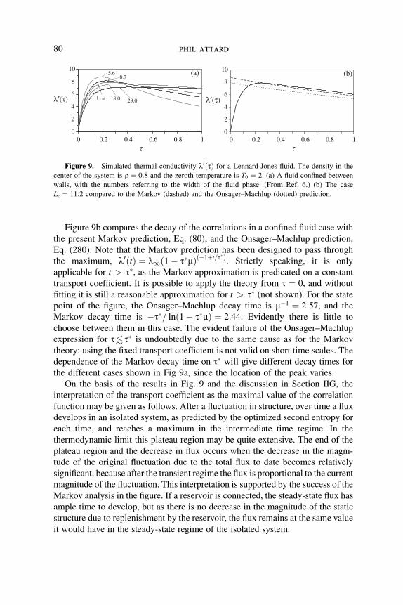
Figure 9b compares the decay of the correlations in a confined fluid case with

the present Markov prediction, Eq. (80), and the Onsager–Machlup prediction,

Eq. (280). Note that the Markov prediction has been designed to pass through

the maximum, l0ðtÞ ¼ l1ð1� t�mÞð�1þt=t�Þ. Strictly speaking, it is only

applicable for t > t�, as the Markov approximation is predicated on a constant

transport coefficient. It is possible to apply the theory from t ¼ 0, and without

fitting it is still a reasonable approximation for t > t� (not shown). For the statepoint of the figure, the Onsager–Machlup decay time is m�1 ¼ 2:57, and the

Markov decay time is �t�= lnð1� t�mÞ ¼ 2:44. Evidently there is little to

choose between them in this case. The evident failure of the Onsager–Machlup

expression for t< t� is undoubtedly due to the same cause as for the Markov

theory: using the fixed transport coefficient is not valid on short time scales. The

dependence of the Markov decay time on t� will give different decay times for

the different cases shown in Fig 9a, since the location of the peak varies.

On the basis of the results in Fig. 9 and the discussion in Section IIG, the

interpretation of the transport coefficient as the maximal value of the correlation

function may be given as follows. After a fluctuation in structure, over time a flux

develops in an isolated system, as predicted by the optimized second entropy for

each time, and reaches a maximum in the intermediate time regime. In the

thermodynamic limit this plateau region may be quite extensive. The end of the

plateau region and the decrease in flux occurs when the decrease in the magni-

tude of the original fluctuation due to the total flux to date becomes relatively

significant, because after the transient regime the flux is proportional to the current

magnitude of the fluctuation. This interpretation is supported by the success of the

Markov analysis in the figure. If a reservoir is connected, the steady-state flux has

ample time to develop, but as there is no decrease in the magnitude of the static

structure due to replenishment by the reservoir, the flux remains at the same value

it would have in the steady-state regime of the isolated system.

0

2

4

6

8

10

10.80.60.40.20

τ

λ′(τ)

5.68.7

11.2 18.0 29.0

(a)

0

2

4

6

8

10

10.80.60.40.20

τ

(b)

λ′(τ)

Figure 9. Simulated thermal conductivity l0ðtÞ for a Lennard-Jones fluid. The density in the

center of the system is r ¼ 0:8 and the zeroth temperature is T0 ¼ 2. (a) A fluid confined between

walls, with the numbers referring to the width of the fluid phase. (From Ref. 6.) (b) The case

Lz ¼ 11:2 compared to the Markov (dashed) and the Onsager–Machlup (dotted) prediction.

80 phil attard

It is also of interest to explore the small-time or transient regime. Using the

functional form t2AðtÞ ¼ si þ jtja2, the second entropy, Eq. (227), may be

extrapolated to smaller time scales. The thermal conductivities become

l0ðtÞ ¼ �tðs1 þ ts2Þ þ

t2s2

ðs1 þ ts2Þ2ð281Þ

and

l00ðtÞ ¼ �t2ðs1 þ ts2Þ ð282Þ

Figure 10 shows small-time fits to the thermal conductivity using the above

functional form. It can be seen that quite good agreement with the simulation

data can be obtained with this simple time-dependent transport function. Such a

function can be used in the transient regime or to characterize the response to

time-varying applied fields.

IX. CONCLUSION

The Second Law of Nonequilibrium Thermodynamics that is described here is

very general. Is it too general to provide a basis for detailed quantitative

calculations? Is there a need for such a law, particularly given its undeniable,

indeed deliberate, similarity, with the traditional equilibrium Second Law?

0

1

2

3

4

5

6

7

8

21.510.50

τ

λ(τ)

Figure 10. Fitted thermal conductivity, l0ðtÞ and l00ðtÞ, using t2AðtÞ ¼ �0:0083� 0:0680jtj,for r ¼ 0:8 (upper data and curves), and t2AðtÞ ¼ �0:139� 0:314jtj, for r ¼ 0:3 (lower data and

curves). (From Ref. 6.)


One of the benefits of having an explicit nonequilibrium Second Law is that

it focuses attention on time, and on the fact that the equilibrium Second Law

offers no prescription for the speed of time or for the rate of change. Similarly,

by introducing the second entropy, which could also be called the transition

entropy, it makes the point that any quantitative theory for the time evolution

of a system must go beyond the ordinary or first entropy. Almost all theories of

the nonequilibrium state to date have been based on the first entropy or its rate

of change. It can be argued that the slow rate of progress of nonequilibrium

theory itself is due directly to the failure to distinguish between the first and

second entropies, a distinction that the nonequilibrium Second Law makes

extant.

Despite the significance of the second entropy, the concept is really very easy

to grasp. The first entropy gives the weight of molecular configurations

associated with the structure that is a macrostate. The second entropy gives the

weight of molecular configurations associated with transitions between pairs of

macrostates. These transitions may be called dynamic structure, and because

they occur over a specified time interval, they are the same as a rate or a flux.

In the equilibrium Second Law, the first entropy increases during spon-

taneous changes in structure, and when the structure stabilizes (i.e., change

ceases), the first entropy is a maximum. This state is called the equilibrium

state. Similarly, in the nonequilibrium Second Law, the second entropy

increases during spontaneous changes in flux, and when the flux stabilizes, the

second entropy is a maximum. This state is called the steady state. The present

nonequilibrium Second Law has the potential to provide the same basis for the

steady state that Clausius’ Second Law has provided for the equilibrium state.

Of course, depending on the system, the optimum state identified by the second

entropy may be the state with zero net transitions, which is just the equilibrium

state. So in this sense the nonequilibrium Second Law encompasses Clausius’

Second Law. The real novelty of the nonequilibrium Second Law is not so much

that it deals with the steady state but rather that it invokes the speed of time

quantitatively. In this sense it is not restricted to steady-state problems, but can in

principle be formulated to include transient and harmonic effects, where the

thermodynamic or mechanical driving forces change with time. The concept of

transitions in the present law is readily generalized to, for example, transitions

between velocity macrostates, which would be called an acceleration, and

spontaneous changes in such accelerations would be accompanied by an increase

in the corresponding entropy. Even more generally it can be applied to a path of

macrostates in time.

Arguably a more practical approach to higher-order nonequilibrium states

lies in statistical mechanics rather than in thermodynamics. The time correlation

function gives the linear response to a time-varying field, and this appears in

computational terms the most useful methodology, even if it may lack the

82 phil attard

satisfying universality of the Second Law. One reason for focussing on the

steady state is the simplicity of many of the analytic formulas that emerge. But

as discussed in Sections IIE and IIG, using the time correlation function itself

can also be fruitful [92].

For nonequilibrium statistical mechanics, the present development of a phase

space probability distribution that properly accounts for exchange with a

reservoir, thermal or otherwise, is a significant advance. In the linear limit the

probability distribution yielded the Green–Kubo theory. From the computational

point of view, the nonequilibrium phase space probability distribution provided

the basis for the first nonequilibrium Monte Carlo algorithm, and this proved to

be not just feasible but actually efficient. Monte Carlo procedures are inherently

more mathematically flexible than molecular dynamics, and the development of

such a nonequilibrium algorithm opens up many, previously intractable, systems

for study. The transition probabilities that form part of the theory likewise

include the influence of the reservoir, and they should provide a fecund basis for

future theoretical research. The application of the theory to molecular-level

problems answers one of the two questions posed in the first paragraph of this

conclusion: the nonequilibrium Second Law does indeed provide a quantitative

basis for the detailed analysis of nonequilibrium problems.

The second question concerned the close similarity between the formulations

of the two Second Laws. The justification for a distinct nonequilibrium Second

Law was given earlier, but the reason for casting it in such a familiar fashion

may be discussed. To some extent, there is no choice in the matter, since as a

law of nature there are only so many ways it can be expressed without changing

its content. Beyond this, there are actually several advantages in the new law

being so closely analogous to the old one. Besides the obvious psychological

fact that familiarity breeds acceptance, familiarity also enables intuition, and so

many nonequilibrium concepts can now be grasped simply by analogy with

their equilibrium counterparts. In fact, in setting up a one-to-one correspon-

dence between the two Second Laws, the groundwork has been laid to carry

over the known equilibrium results to the nonequilibrium context. That is, all

known equilibrium principles, theorems, and relationships ought to have a

nonequilibrium version based on the correspondence established by the new

Second Law.

The philosophical and conceptual ramifications of the nonequilibrium

Second Law are very deep. Having established the credentials of the Law by

the detailed analysis outlined earlier, it is worth considering some of these large-

scale consequences. Whereas the equilibrium Second Law of Thermodynamics

implies that order decreases over time, the nonequilibrium Second Law of

Thermodynamics explains how it is possible that order can be induced and how

it can increase over time. The question is of course of some relevance to the

creation and evolution of life, society, and the environment.


The present analysis shows that when a thermodynamic gradient is first

applied to a system, there is a transient regime in which dynamic order is

induced and in which the dynamic order increases over time. The driving force

for this is the dissipation of first entropy (i.e., reduction in the gradient), and

what opposes it is the cost of the dynamic order. The second entropy provides a

quantitative expression for these processes. In the nonlinear regime, the fluxes

couple to the static structure, and structural order can be induced as well. The

nature of this combined order is to dissipate first entropy, and in the transient

regime the rate of dissipation increases with the evolution of the system over

time.

Prigogine has used the term ‘‘dissipative structures’’ to describe the order

induced during nonequilibrium processes [11, 83]. Physical examples include

convective rolls, chemical clock reactions, and chaotic flows. These are also

suggested to be related to the type of order that living organisms display—a

theme that continues to be widely studied [13–18]. While one can argue about

the mathematical analysis and physical interpretation of these studies, there is

little doubt that the broad picture that emerges is consistent with the

nonequilibrium Second Law. At its simplest, the argument is that life exists

on the energy gradient provided by the Sun. Living systems also exploit

gradients in material resources due to their spatial segregation. The raison d’etre

for life is to reduce these gradients, and the role of evolution is to increase

the rate at which these gradients are dissipated. Cope’s rule, which is the

observation that body size increases as species evolve [93], may simply be a

manifestation of the extensivity of the second entropy. Changes in environment

and society occur on shorter time scales than biological evolution, and the

historical record certainly reveals an increasing capacity for entropy production

over time. It is sobering to reflect that we evolve in order to hasten our own end.

Acknowledgments

Angus Gray-Weale is thanked for useful discussions on the symmetry and time dependence of the

transport coefficients, and the Australian Research Council is thanked for financial support.

References

1. P. Attard, J. Chem. Phys. 121, 7076 (2004).

2. P. Attard, J. Chem. Phys. 122 154101 (2005).






8. P. Attard, Phys. Chem. Chem. Phys. 8, 3585 (2006).

84 phil attard

9. P. Attard, Thermodynamics and Statistical Mechanics: Equilibrium by Entropy Maximisation,

Academic Press, London, 2002.

10. L. Onsager, Phys. Rev. 37, 405 (1931); 38, 2265 (1931).

11. I. Prigogine, Introduction to Thermodynamics of Irreversible Processes, Interscience,

New York, 1967.

12. S. R. de Groot and P. Mazur, Non-equilibrium Thermodynamics, North-Holland, Amsterdam,

1969.

13. G. W. Paltridge, Nature 279, 630 (1979).

14. R. Swenson and M. T. Turvey, Ecological Psychol. 3, 317 (1991).

15. E. D. Schneider and J. J. Kay, Math. Comp. Mod. 19, 25 (1994).

16. R. Dewar, J. Phys. Math. Gen. 36, 631 (2003).

17. A. Kleidon and R. D. Lorenz (eds.), Non-equilibrium Thermodynamics and the Production of

Entropy: Life, Earth, and Beyond, Springer, Berlin, 2005.

18. L. M. Martyushev and V. D. Seleznev, Phys. Rep. 426, 1 (2006).

19. M. Paniconi and Y. Oono, Phys. Rev. E 55, 176 (1997).

20. Y. Oono and M. Paniconi, Prog. Theor. Phys. Suppl. 130, 29 (1998).

21. B. C. Eu, Nonequilibrium Statistical Mechanics, Kluwer Academic Publishers, Dordrecht,

1998.

22. D. Jou, J. Casa-Vazquez, and G. Lebon, Rep. Prog. Phys. 62, 1035 (1999).

23. J. Casa-Vazquez and D. Jou, Rep. Prog. Phys. 66, 1937 (2003).

24. H. B. G. Casimir, Rev. Mod. Phys. 17, 343 (1945).

25. H. Grabert, R. Graham, and M. S. Green, Phys. Rev. A 21, 2136 (1980).

26. M. S. Green, J. Chem. Phys. 22, 398 (1954).

27. R. Kubo, Rep. Prog. Phys. 29, 255 (1966).

28. J.-P. Hansen and I. R. McDonald, Theory of Simple Liquids, Academic Press, London, 1986.

29. J. P. Boon and S. Yip, Molecular Hydrodynamics, Dover, New York, 1991.

30. R. Zwanzig, Non-equilibrium Statistical Mecahnics, Oxford University Press, Oxford, UK,

2001.

31. H. B. Callen and R. F. Greene, Phys. Rev. 86, 702 (1952). R. F. Greene and H. B. Callen, Phys.

Rev. 88, 1387 (1952).

32. L. Onsager and S. Machlup, Phys. Rev. 91, 1505 (1953).

33. H. Risken, The Fokker–Planck Equation, Springer-Verlag, Berlin, 1984.

34. R. L. Stratonovich, Sel. Transl. Math. Stat. Prob. 10, 273 (1971).

35. J. Keizer, Statistical Thermodynamics of Nonequilibrium Processes, Springer-Verlag,

New York, 1987.

36. W. Horsthemke and A. Bach, Z. Phys. B 22, 189 (1975).

37. H. Haken, Z. Phys. B 24, 321 (1976).

38. R. Graham, Z. Phys. B 26, 281 (1977).

39. K. Yasue, J. Math. Phys. 19, 1671 (1978).

40. H. Grabert and M. S. Green, Phys. Rev. A 19, 1747 (1979).

41. B. H. Lavenda, Foundations Phys. 9, 405 (1979).

42. K. L. C. Hunt and J. Ross, J. Chem. Phys. 75, 976 (1981).

43. B. H. Lavenda, Nonequilibrium Statistical Thermodynamics, Wiley, Chichester, 1985.


44. G. L. Eyink, J. Stat. Phys. 61, 533 (1990).

45. B. Peng, K. L. C. Hunt, P. M. Hunt, A. Suarez, and J. Ross, J. Chem. Phys. 102, 4548 (1995).

46. P. Ao, J. Phys. A Math. Gen. 37, L25 (2004).

47. N. Hashitsume, Prog. Theor. Phys. 8, 461 (1952).

48. I. Gyarmati, Z. Phys. Chem. Leipzig 239, 133 (1968).

49. I. Gyarmati, Nonequilibrium Thermodynamics, Field Theory, and Variational Principles,

Springer, Berlin, 1970.

50. G. N. Bochkov and Yu. E. Kuzovlev, JETP Lett. 30, 46 (1980).

51. D. J. Evans and A. Baranyai, Phys. Rev. Lett. 67, 2597 (1991).

52. A. Baranyai, J. Chem. Phys. 105, 7723 (1996).

53. D. J. Evans and G. P. Morriss, Statistical Mechanics of Nonequilibrium Liquids, Academic,

London, 1990.

54. W. H. Hoover, Computational Statistical Mechanics, Elsevier, Amsterdam, 1991.

55. C. Jarzynski, Phys. Rev. Lett. 78, 2690 (1997).

56. D. J. Evans, E. G. D. Cohen, and G. P. Morriss, Phys. Rev. Lett. 71, 2401 (1993).

57. D. J. Evans, Mol. Phys. 101, 1551 (2003).

58. G. N. Bochkov and Yu. E. Kuzovlev, Sov. Phys. JETP 45, 125 (1977).

59. G. N. Bochkov and Yu. E. Kuzovlev, Sov. Phys. JETP 49, 543 (1977).

60. G. N. Bochkov and Yu. E. Kuzovlev, Physica 106A, 443 (1981).

61. G. E. Crooks, Phys. Rev. E 60, 2721 (1999).

62. G. E. Crooks, Phys. Rev. E 61, 2361 (2000).

63. G. M.Wang, E. M. Sevick, E. Mittag, D. J. Searles, and D. J. Evans, Phys. Rev. Lett. 89, 050601

(2002).

64. C. Jarzynski, Phys. Rev. E 56, 5018 (1997).

65. G. E. Crooks, J. Stat. Phys. 90, 1481 (1998).

66. J. Liphardt, S. Dumont, S. B. Smith, I. Tinoco Jr., and C. Bustamante, Science 296, 1832 (2002).

67. R. P. Feynman, Statistical Mechanics: A Set of Lectures, Benjamin, Reading, MA, 1972.

68. T. Yamada and K. Kawasaki, Prog. Theor. Phys. 38, 1031 (1967).

69. T. Yamada and K. Kawasaki, Prog. Theor. Phys. 53, 111 (1975).

70. G. P. Morriss and D. J. Evans, Mol. Phys. 54, 629 (1985).

71. G. P. Morriss and D. J. Evans, Phys. Rev. A 37, 3605 (1988).

72. T. Hatano and S. Sasa, Phys. Rev. Lett. 86, 3463 (2001).

73. E. H. Trepagnier, C. Jarzynski, F. Rotort, G. E. Crooks, C. J. Bustamante, and J. Liphardt, PNAS

101, 15038 (2004).

74. O. Mazonka and C. Jarzynski, arXiv:cond-mat/9912121 (1999).

75. R. J. Glauber, J. Math. Phys. 4, 294 (1963).

76. K. Kawasaki, Phys. Rev. 145, 145 (1966).

77. J. S. Langer, Ann. Phys. 54, 258 (1969).

78. H. Metiu, K. Kitahara, and J. Ross, J. Chem. Phys. 63, 5116 (1975).

79. H. C. Anderson, J. Chem. Phys. 72, 2384 (1980).


81. S. Boinepalli and P. Attard, J. Chem. Phys. 119, 12769 (2003).

82. R. F. Fox and G. E. Uhlenbeck, Phys. Fluids 13, 1893 (1970).

86 phil attard

83. I. Prigogine, Time, Structure, and Fluctuations, Nobel Lecture, 1977.

84. M. P. Allen and D. J. Tildesley, Computer Simulation of Liquids, Oxford University Press,

Oxford, UK, 1987.

85. B. L. Holian, G. Ciccotti, W. G. Hoover, B. Moran, and H. A. Posch, Phys. Rev. A 39, 5414

(1989).

86. G. P. Morriss, Phys. Rev. A 39, 4811 (1989).

87. D. J. Evans and D. J. Searles, Phys. Rev. E 52, 5839 (1995).

88. D. J. Evans and G. P. Morriss, Comput. Phys. Rep. 1, 297 (1984).

89. P. J. Daivis and D. J. Evans, Phys. Rev. E 48, 1058 (1993).

90. J. K. Johnson, J. A. Zollweg, and K. E. Gubbins, Mol. Phys. 78, 591 (1993).

91. D. J. Evans, Phys. Rev. A 34, 1449 (1986).

92. A. Gray-Weale and P. Attard, J. Chem. Phys. 127, 044503 (2007).

93. W. H. Gould, Hens Teeth and Horse’s Toes: Further Reflections on Natural History, Norton,

New York, 1983.


the second law of nonequilibrium thermodynamics - personal pages

Documents