the science and art of structural...

1

The Science and Art of StructuralDynamics

What do a sport-utility vehicle traveling off-road, an airplane flying near a thunderstorm,an offshore oil platform in rough seas, and an office tower during an earthquake allhave in common? One answer is that all of these are structures that are subjected todynamic loading, that is, to time-varying loading. The emphasis placed on the safety,performance, and reliability of mechanical and civil structures such as these has ledto the need for extensive analysis and testing to determine their response to dynamicloading. The structural dynamics techniques that are discussed in this book have evenbeen employed to study the dynamics of snow skis and violins.

Although the topic of this book, as indicated by its title, is structural dynamics,some books with the word vibrations in their title discuss essentially the same subjectmatter. Powerful computer programs are invariably used to implement the modeling,analysis, and testing tasks that are discussed in this book, whether the applicationis one in aerospace engineering, civil engineering, mechanical engineering, electricalengineering, or even in sports or music.

1.1 INTRODUCTION TO STRUCTURAL DYNAMICS

This introductory chapter is entitled “The Science and Art of Structural Dynamics”to emphasize at the outset that by studying the principles and mathematical formulasdiscussed in this book you will begin to understand the science of structural dynamicsanalysis. However, structural dynamicists must also master the art of creating mathe-matical models of structures, and in many cases they must also perform dynamic tests.The cover photo depicts an automobile that is undergoing such dynamic testing. Mod-eling, analysis, and testing tasks all demand that skill and judgment be exercised inorder that useful results will be obtained; and all three of these tasks are discussed inthis book.

A dynamic load is one whose magnitude, direction, or point of application varieswith time. The resulting time-varying displacements and stresses constitute the dynamicresponse. If the loading is a known function of time, the loading is said to be prescribedloading, and the analysis of a given structural system to a prescribed loading is calleda deterministic analysis. If the time history of the loading is not known completely butonly in a statistical sense, the loading is said to be random. In this book we treat onlyprescribed dynamic loading.

1

COPYRIG

HTED M

ATERIAL

2 The Science and Art of Structural Dynamics

P P(t)

Distributedinertia force

(a) (b)

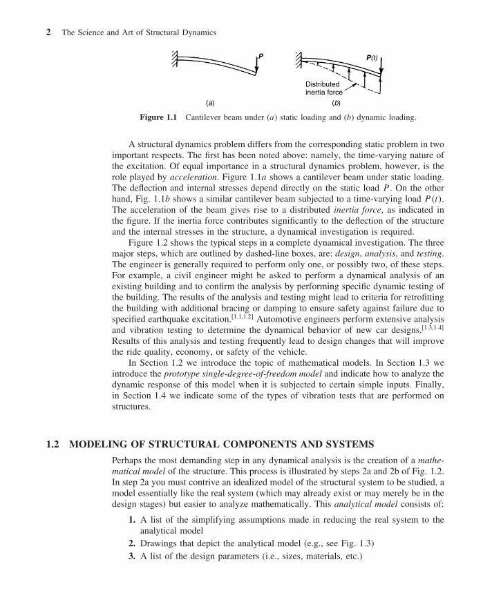
Figure 1.1 Cantilever beam under (a) static loading and (b) dynamic loading.

A structural dynamics problem differs from the corresponding static problem in twoimportant respects. The first has been noted above: namely, the time-varying nature ofthe excitation. Of equal importance in a structural dynamics problem, however, is therole played by acceleration. Figure 1.1a shows a cantilever beam under static loading.The deflection and internal stresses depend directly on the static load P . On the otherhand, Fig. 1.1b shows a similar cantilever beam subjected to a time-varying load P(t).The acceleration of the beam gives rise to a distributed inertia force, as indicated inthe figure. If the inertia force contributes significantly to the deflection of the structureand the internal stresses in the structure, a dynamical investigation is required.

Figure 1.2 shows the typical steps in a complete dynamical investigation. The threemajor steps, which are outlined by dashed-line boxes, are: design, analysis, and testing.The engineer is generally required to perform only one, or possibly two, of these steps.For example, a civil engineer might be asked to perform a dynamical analysis of anexisting building and to confirm the analysis by performing specific dynamic testing ofthe building. The results of the analysis and testing might lead to criteria for retrofittingthe building with additional bracing or damping to ensure safety against failure due tospecified earthquake excitation.[1.1,1.2] Automotive engineers perform extensive analysisand vibration testing to determine the dynamical behavior of new car designs.[1.3,1.4]

Results of this analysis and testing frequently lead to design changes that will improvethe ride quality, economy, or safety of the vehicle.

In Section 1.2 we introduce the topic of mathematical models. In Section 1.3 weintroduce the prototype single-degree-of-freedom model and indicate how to analyze thedynamic response of this model when it is subjected to certain simple inputs. Finally,in Section 1.4 we indicate some of the types of vibration tests that are performed onstructures.

1.2 MODELING OF STRUCTURAL COMPONENTS AND SYSTEMS

Perhaps the most demanding step in any dynamical analysis is the creation of a mathe-matical model of the structure. This process is illustrated by steps 2a and 2b of Fig. 1.2.In step 2a you must contrive an idealized model of the structural system to be studied, amodel essentially like the real system (which may already exist or may merely be in thedesign stages) but easier to analyze mathematically. This analytical model consists of:

1. A list of the simplifying assumptions made in reducing the real system to theanalytical model

2. Drawings that depict the analytical model (e.g., see Fig. 1.3)3. A list of the design parameters (i.e., sizes, materials, etc.)

Sta

rt

1E

XIS

TIN

GS

TR

UC

TU

RE

or D

esig

nD

raw

ings

and

Dat

aD

ES

IGN

AN

ALY

SIS

TE

ST

ING

RE

DE

SIG

N

No

Yes

No

No

No

Yes

Yes

Yes

Ana

lytic

alm

odel

OK

?

Str

uctu

reav

aila

ble

?

Des

ign

chan

ges

?S

top

Test

?

AN

ALY

TIC

AL

MO

DE

L(A

ssum

ptio

ns,

sket

ches

, etc

.)

2bM

ATH

EM

ATIC

AL

MO

DE

L(D

iffer

entia

leq

uatio

ns)

(Ass

umpt

ions

, etc

.)

6aD

ES

IGN

CH

AN

GE

S

4P

HY

SIC

AL

MO

DE

L

3 D

YN

AM

ICA

LB

EH

AV

IOR

(Sol

utio

n of

DE

s)

DE

SIG

NC

HA

NG

ES

6b2a

DY

NA

MIC

AL

TE

ST

ING

5

(Par

amet

er c

hang

es)

Fig

ure

1.2

Step

sin

ady

nam

ical

inve

stig

atio

n.

3


v(x,t)

x

v(t)

v1(t)v2(t)

v3(t)

(a)

(b)

(c)

Figure 1.3 Analytical models of a cantilever beam: (a) distributed-mass cantilever beam, acontinuous model (or distributed-parameter model); (b) one-degree-of-freedom model, a discrete-parameter model; (c) three-degree-of-freedom model, a more refined discrete-parameter model.

Analytical models fall into two basic categories: continuous models and discrete-parameter models. Figure 1.3a shows a continuous model of a cantilever beam. Thenumber of displacement quantities that must be considered to represent the effectsof all significant inertia forces is called the number of degrees of freedom (DOF) ofthe system. Thus, a continuous model represents an infinite-DOF system. Techniquesfor creating continuous models are discussed in Chapter 12. However, Fig. 1.3b andc depict finite-DOF systems. The discrete-parameter models shown here are calledlumped-mass models because the mass of the system is assumed to be represented by asmall number of point masses, or particles. Techniques for creating discrete-parametermodels are discussed in Chapters 2, 8, and 14.

To create a useful analytical model, you must have clearly in mind the intendeduse of the analytical model, that is, the types of behavior of the real system that themodel is supposed to represent faithfully. The complexity of the analytical model isdetermined (1) by the types and detail of behavior that it must represent, (2) by thecomputational analysis capability available (hardware and software), and (3) by the timeand expense allowable. For example, Fig. 1.4 shows four different analytical modelsused in the 1960s to study the dynamical behavior of the Apollo Saturn V space vehicle,the vehicle that was used in landing astronauts on the surface of the moon. The 30-DOFbeam-rod model was used for preliminary studies and to determine full-scale testingrequirements. The 300-DOF model on the right, on the other hand, was required to give

1.2 Modeling of Structural Components and Systems 5

30 DOF

ApolloSatum V

spacevehicle

Beam-rodmodel

Beam-rodquarter-

shellmodel

Quarter-shell

model

Three- dimensional

model

120 DOF 400 DOF 300 DOF

Figure 1.4 Analytical models of varying complexity used in studying the space vehicle dynam-ics of the Apollo Saturn V. (From C. E. Green et al., Dynamic Testing for Shuttle DesignVerification, NASA, Washington, DC, 1972.)

a more accurate description of motion at the flight sensor locations. All of these Saturn Vanalytical models are extremely small compared with the multimillion-DOF models thatcan be analyzed now (see Section 17.8). However, supported by extensive dynamicaltesting, these analytical models were sufficient to ensure successful accomplishment ofApollo V ’s moon-landing mission. Simplicity of the analytical model is very desirableas long as the model is adequate to represent the necessary behavior.

Once you have created an analytical model of the structure you wish to study, youcan apply physical laws (e.g., Newton’s Laws, stress–strain relationships) to obtainthe differential equation(s) of motion that describe, in mathematical language, the ana-lytical model. A continuous model leads to partial differential equations, whereas adiscrete-parameter model leads to ordinary differential equations. The set of differentialequations of motion so derived is called a mathematical model of the structure. To obtaina mathematical model, you will use methods studied in dynamics (e.g., Newton’s Laws,Lagrange’s Equations) and in mechanics of deformable solids (e.g., strain–displacementrelations, stress–strain relations) and will combine these to obtain differential equationsdescribing the dynamical behavior of a deformable structure.


In practice you will find that the entire process of creating first an analytical modeland then a mathematical model may be referred to simply as mathematical modeling.In using a finite element computer program such as ABAQUS[1.5], ANSYS[1.6], MSC-Nastran[1.7], OpenFEM[1.8], SAP2000[1.9], or another computer program to carry out astructural dynamics analysis, your major modeling task will be to simplify the systemand provide input data on dimensions, material properties, loads, and so on. This is

(a)

(b)

Figure 1.5 (a) Actual bus body and frame structure; (b) finite element models of the body andframe. (From D. Radaj et al., Finite Element Analysis: An Automobile Engineer’s Tool, Societyof Automotive Engineers, 1974. Used with permission of the Society of Automotive Engineers,Inc. Copyright c© 1974 SAE.)

1.3 Prototype Spring–Mass Model 7

where the “art” of structural dynamics comes into play. On the other hand, actualcreation and solution of the differential equations is done by the computer program.Figure 1.5 shows a picture of an actual bus body and a computer-generated plot of theidealized structure, that is, analytical model, which was input to a computer. Computergraphics software (e.g., MSC-Patran[1.7]) has become an invaluable tool for use increating mathematical models of structures and in displaying the results of the analysesthat are performed by computers.

Once a mathematical model has been formulated, the next step in a dynamicalanalysis is to solve the differential equation(s) to obtain the dynamical response that ispredicted. (Note: The terms dynamical response and vibration are used interchangeably.)The two types of dynamical behavior that are of primary importance in structuralapplications are free vibration and forced vibration (or forced response), the formerbeing the motion resulting from specified initial conditions, and the latter being themotion resulting directly from specified inputs to the system from external sources.Thus, you solve the differential equations of motion subject to specified initial conditionsand to specified inputs from external sources, and you obtain the resulting time historiesof the motion of the structure and stresses within the structure. This constitutes thebehavior predicted for the (real) structure, or the response.

The analysis phase of a dynamical investigation consists of the three stepsjust described: defining the analytical model, deriving the corresponding mathemati-cal model, and solving for the dynamical response. This book deals primarily withthe second and third steps in the analysis phase of a structural dynamics investigation.Section 1.3 illustrates these steps for the simplest analytical model, a lumped-masssingle-DOF model. Section 1.4 provides a brief discussion of dynamical testing.

1.3 PROTOTYPE SPRING–MASS MODEL

Before proceeding with the details of how to model complex structures and analyze theirdynamical behavior, let us consider the simplest structure undergoing the simplest formsof vibration. The structure must have an elastic component, which can store and releasepotential energy; and it must have mass, which can store and release kinetic energy.The simplest model, therefore, is the spring–mass oscillator, shown in Fig. 1.6a.

1.3.1 Simplifying Assumptions: Analytical Model

The simplifying assumptions that define this prototype analytical model are:

1. The mass is a point mass that is confined to move along one horizontal directionon a frictionless plane. The displacement of the mass in the x direction fromthe position where the spring is undeformed is designated by the displacementvariable u(t).

2. The mass is connected to a fixed base by an idealized massless, linear spring.The fixed base serves as an inertial reference frame. Figure 1.6b shows the linearrelationship between the elongation (u positive) and contraction (u negative) ofthe spring and the force fS(t) that the spring exerts on the mass. When thespring is in tension, fS is positive; when the spring is in compression, fS isnegative.

3. A specified external force p(t) acts on the mass, as shown in Fig. 1.6a.


x

k

mp(t)

u(t)

(a)

fS

u

kl

(b)

mfS

u(t)

p(t)

(c)

Figure 1.6 (a) Spring–mass oscillator; (b) force–elongation behavior of a linear spring; (c)free-body diagram of the spring–mass oscillator.

Since it takes only one variable [e.g., u(t)] to specify the instantaneous position ofthe mass, this is called a single-degree-of-freedom (SDOF) system.

1.3.2 Mathematical Model: Equation of Motion

Newton’s Second Law To obtain a mathematical model describing the behavior of thespring–mass oscillator, we start by drawing a free-body diagram of the mass (Fig. 1.6c)and applying Newton’s Second Law,

∑Fx = max (1.1)

where m is the mass and ax is the acceleration of the mass, taken as positive in the+x direction. Acceleration ax is given by the second derivative of the displacement,that is, ax = u(t); similarly, the velocity is given by u(t). By assuming that the mass


is displaced u to the right of the position where the spring force is zero, we can saythat the spring will be in tension, so the spring force will act to the left on the mass,as shown on the free-body diagram. Thus, Eq. 1.1 becomes

−fS + p(t) = mu (1.2)

Force–Displacement Relationship As indicated in Fig. 1.6b, there is assumed to bea linear relationship between the force in the spring and its elongation u, so

fS = ku (1.3)

where k is the stiffness of the spring.Equation of Motion Finally, by combining Eqs. 1.2 and 1.3 and rearranging to placeall u-terms on the left, we obtain the equation of motion for the prototype undampedSDOF model:

mu + ku = p(t) (1.4)

This equation of motion is a linear second-order ordinary differential equation. It is themathematical model of this simple SDOF system.

Having Eq. 1.4, the equation of motion that governs the motion of the SDOFspring–mass oscillator in Fig. 1.6a, we now examine the dynamic response of thisprototype system. The response of the system is determined by its initial conditions,that is, by the values of its displacement and velocity at time t = 0:

u(0) = u0 = initial displacement, u(0) = v0 = initial velocity (1.5)

and by p(t), the external force acting on the system. Here we consider two simpleexamples of vibration of the spring–mass oscillator; a more general discussion ofSDOF systems follows in Chapters 3 through 7.

1.3.3 Free Vibration Example

The spring–mass oscillator is said to undergo free vibration if p(t) ≡ 0, but the masshas nonzero initial displacement u0 and/or nonzero initial velocity v0. Therefore, theequation of motion for free vibration is the homogeneous second-order differentialequation

mu + ku = 0 (1.6)

The general solution of this well-known simple differential equation is

u = A1 cos ωnt + A2 sin ωnt (1.7)

where ωn is the undamped circular natural frequency, defined by

ωn =√

k

m(1.8)

The units of ωn are radians per second (rad/s).


The constants A1 and A2 in Eq. 1.7 are chosen so that the two initial conditions,Eqs. 1.5, will be satisfied. Thus, free vibration of an undamped spring–mass oscillatoris characterized by the time-dependent displacement

u(t) = u0 cos ωnt + v0

ωn

sin ωnt (1.9)

It is easy to show that this solution satisfies the differential equation, Eq. 1.6, and thetwo initial conditions, Eqs. 1.5.

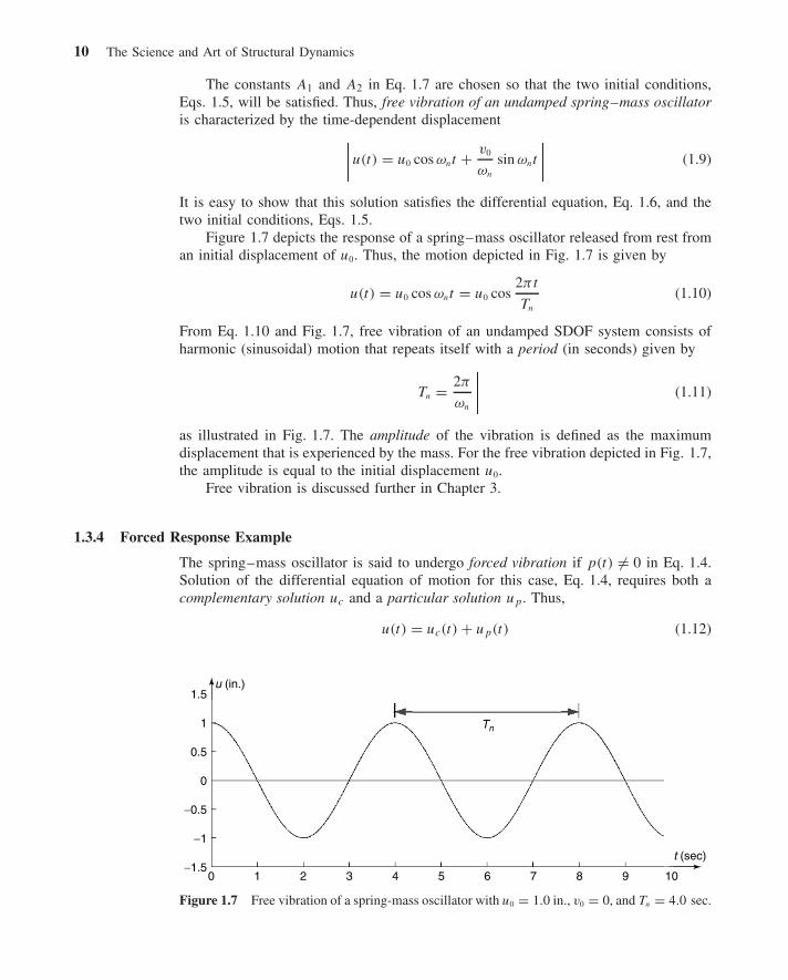
Figure 1.7 depicts the response of a spring–mass oscillator released from rest froman initial displacement of u0. Thus, the motion depicted in Fig. 1.7 is given by

u(t) = u0 cos ωnt = u0 cos2πt

Tn

(1.10)

From Eq. 1.10 and Fig. 1.7, free vibration of an undamped SDOF system consists ofharmonic (sinusoidal) motion that repeats itself with a period (in seconds) given by

Tn = 2π

ωn

(1.11)

as illustrated in Fig. 1.7. The amplitude of the vibration is defined as the maximumdisplacement that is experienced by the mass. For the free vibration depicted in Fig. 1.7,the amplitude is equal to the initial displacement u0.

Free vibration is discussed further in Chapter 3.

1.3.4 Forced Response Example

The spring–mass oscillator is said to undergo forced vibration if p(t) �= 0 in Eq. 1.4.Solution of the differential equation of motion for this case, Eq. 1.4, requires both acomplementary solution uc and a particular solution up. Thus,

u(t) = uc(t) + up(t) (1.12)

1.5

0 1 2 3 4 5 6 7 8 9 10

1

0.5

0

−0.5

−1

−1.5

Tn

t (sec)

u (in.)

Figure 1.7 Free vibration of a spring-mass oscillator with u0 = 1.0 in., v0 = 0, and Tn = 4.0 sec.


As a simple illustration of forced vibration we consider ramp response, the responseof the spring–mass oscillator to the linearly varying ramp excitation force given by

p(t) = p0

t

t0

, t > 0 (1.13)

and illustrated in Fig. 1.8a. (The time t0 is the time at which the force reaches thevalue p0.) The particular solution, like the excitation, varies linearly with time. Thecomplementary solution has the same form as given in Eq. 1.7, so the total responsehas the form

u(t) = A1 cos ωnt + A2 sin ωnt + p0

k

t

t0

(1.14)

where the constants A1 and A2 must be selected so that the initial conditions u(0) andu(0) will be satisfied.

Figure 1.8b depicts the response of a spring–mass oscillator that is initially at restat the origin, so the initial conditions are u(0) = u(0) = 0. The corresponding rampresponse is thus given by

u(t) = p0

k

(t

t0

− 1

ωnt0

sin ωnt

)(1.15)

t (sec)

0 2 4 6 8 100

0.5

1

1.5

2

u (in.)

0 2 4 6 8 100

0.5

1

1.5

2

t (sec)

p (lb)

(a)

(b)

Figure 1.8 (a) Ramp excitation p(t) = p0(t/t0) for t > 0, with p0 = 2 lb, t0 = 10 sec; (b)response of a spring–mass oscillator to ramp excitation. For (b), k = 1 lb/in. and Tn = 4 sec.


Clearly evident in this example of forced response are two components: (1) a linearlytime-varying displacement (dashed curve), which is due directly to the linearly time-varying ramp excitation, and (2) an induced oscillatory motion at the undamped naturalfrequency ωn. Of course, this ramp response is only valid as long as the spring remainswithin its linearly elastic range.

1.3.5 Conclusions

In this section we have taken a preliminary look at several characteristics that aretypical of the response of structures to nonzero initial conditions and/or to time-varyingexcitation. We have especially noted the oscillatory nature of the response. In Chapters 3through 7, we consider many additional examples of free and forced vibration of SDOFsystems, including systems with damping.

1.4 VIBRATION TESTING OF STRUCTURES

A primary purpose of dynamical testing is to confirm a mathematical model and, inmany instances, to obtain important information on loads, on damping, and on otherquantities that may be required in the dynamical analysis. In some instances thesetests are conducted on reduced-scale physical models: for example, wind tunnel testsof airplane models. In other cases, when a full-scale structure (e.g., an automobile) isavailable, the tests may be conducted on it.

Aerospace vehicles (i.e., airplanes, spacecraft, etc.) must be subjected to extensivestatic and dynamic testing on the ground prior to actual flight of the vehicle. Figure 1.9a

shows a ground vibration test in progress on a Boeing 767 airplane. Note the electro-dynamic shaker in place under each wingtip and the special soft support under the noselanding gear.

Dynamical testing of physical models may be employed for determining qualita-tively and quantitatively the dynamical behavior characteristics of a particular class ofstructures. For example, Fig. 1.9b shows an aeroelastic model of a Boeing 777 airplaneundergoing ground vibration testing in preparation for testing in a wind tunnel to aid inpredicting the dynamics of the full-scale airplane in flight. Note the soft bungee-corddistributed support of the model and the two electrodynamic shakers that are attachedby stingers to the engine nacelles. Figure 1.10 shows a fluid-filled cylindrical tank struc-ture in place on a shake table in a university laboratory. The shake table is used tosimulate earthquake excitation at the base of the tank structure.

Chapter 18 provides an introduction to Experimental Modal Analysis, a very impor-tant structural dynamics test procedure that is used extensively in the automotive andaerospace industries and is also used to test buildings, bridges, and other civil structures.

1.5 SCOPE OF THE BOOK

Part I, encompassing Chapters 2 through 7, treats single-degree-of-freedom (SDOF)systems. In Chapter 2 procedures are described for developing SDOF mathematicalmodels; both Newton’s Laws and the Principle of Virtual Displacements are employed.The free vibration of undamped and damped systems is the topic of Chapter 3, and

1.5 Scope of the Book 13

(a)

(b)

Figure 1.9 (a) Ground vibration testing of the Boeing 767 airplane; (b) aeroelastic wind-tunnelmodel of the Boeing 777 airplane. (Courtesy of Boeing Commercial Airplane Company.)

in Chapter 4 you will learn about the response of SDOF systems to harmonic (i.e.,sinusoidal) excitation. This is, perhaps, the most important topic in the entire book,because it describes the fundamental characteristics of the dynamic response of flexiblestructures. Chapters 5 and 6 continue the discussion of dynamic response of SDOFsystems. In Chapter 5 we treat closed-form methods for evaluating the response ofSDOF systems to nonperiodic inputs, and Chapter 6 deals with numerical techniques.Part I concludes with Chapter 7, where the response of SDOF systems to periodicexcitation is considered. Frequency-domain techniques, which are currently used widely


Figure 1.10 Fluid-filled tank subjected to simulated earthquake excitation. (Courtesy of R. W.Clough.)

in dynamic testing of structures, are introduced as a natural extension of the discussionof periodic excitation.

Analysis of the dynamical behavior of structures of even moderate complexityrequires the use of multiple-degree-of-freedom (MDOF) models. Part II, which consistsof Chapters 8 through 11, discusses procedures for obtaining MDOF mathematical mod-els and for analyzing their free- and forced-vibration response. Mathematical modelingis treated in Chapter 8. While Newton’s Laws can be used to derive mathemati-cal models of some MDOF systems, the primary procedure employed for derivingsuch models is the use of Lagrange’s Equations. Continuous systems are approximatedby MDOF models through the use of the Assumed-Modes Method. Chapter 9, whichtreats vibration of undamped two-degree-of-freedom (2-DOF) systems, introduces manyof the concepts that are important to a study of the response of MDOF systems: forexample, natural frequencies, normal modes, and mode superposition. In Chapter 10we discuss many of the mathematical properties related to modes and frequencies ofboth undamped and damped MDOF systems and introduce several popular schemesfor representing damping in structures. In addition, the subject of complex modes isintroduced in Chapter 10. Finally, in Chapter 11 we discuss mode superposition, themost widely used procedure for determining the response of MDOF systems.

Part III treats structures that are modeled as continuous systems. Although importanttopics such as the determination of partial differential equation mathematical models

1.6 Computer Simulations; Supplementary Material on the Website 15

(Chapter 12) and determination of modes and frequencies (Chapter 13) are discussed,the primary purpose of Part III is to provide several “exact solutions” that can be usedfor evaluating the accuracy of the approximate MDOF models analyzed in Parts IIand IV.

Part IV presents computational techniques for handling structural dynamics appli-cations in engineering by the methods that are widely used for analyzing and testingthe behavior of complex structures (e.g., airplanes, automobiles, high-rise buildings). InChapter 14, a continuation of the mathematical modeling topics in Chapter 8, you areintroduced to the important Finite Element Method (FEM) for creating MDOF mathe-matical models. Chapter 14 also includes several FEM examples involving mode shapesand natural frequencies, extending the discussion of those topics in Chapters 9 and 10.Prior study of the Finite Element Method, or of Matrix Structural Analysis, is not aprerequisite for Chapter 14. Chapters 15 through 17 treat advanced numerical methodsfor solving structural dynamics problems: eigensolvers for determining modes and fre-quencies of complex structures (Chapter 15), direct integration methods for computingdynamic response (Chapter 16), and substructuring (Chapter 17).

Finally, in Part V, Chapters 18 through 20, we introduce advanced structuraldynamics applications: experimental modal analysis, or modal testing (Chapter 18);structures containing piezoelectric members, or “active structures” (Chapter 19); andearthquake response of structures (Chapter 20).

A reader who merely wishes to attain an introductory level of understanding ofcurrent structural dynamics analysis techniques need only study Chapters 2 through 11and Chapter 14.

1.6 COMPUTER SIMULATIONS; SUPPLEMENTARY MATERIALON THE WEBSITE

The objective of this book is to introduce you to computer methods in structural dynam-ics. Therefore, most chapters contain computer plots of one or more of the following:mode shapes, response time histories, frequency-response functions, and so on. Someof these are plots of closed-form mathematical expressions; others are generated byalgorithms that are presented in the text. Also, a number of homework problems askfor similar computer-generated results.

To facilitate your understanding of the procedures discussed in the book, a num-ber of supplementary materials are made available to you on the book’s websitewww.wiley.com/college/craig. Included are the following:

• Matlab1 .m-files that were used to create the plots included in this book, andMatlab .m-files for many of the numerical analysis algorithms presented inChapters 6, 7, 15, and 16.

• Line drawings and plots in the form of .eps files.• ISMIS, a Matlab-based matrix structural analysis computer program. Included

are the Matlab .m-files, a .pdf file entitled Special ISMIS Operations for Struc-tural Analysis, and two ISMIS examples. This software supplements Chapter 14.

1Matlab is the most widely used computer software for solving dynamics problems, including structuraldynamics problems of the size and scope of those in this book[1.10]. If you are inexperienced in the use ofMatlab, you should read Appendix E, “Introduction to the Use of Matlab,” in its entirety.


• TUTORIAL NOTES: Structural Dynamics and Experimental Modal Analysis byPeter Avitabile. These short course notes supplement Chapter 18.

• “Airplane Ground Vibration Testing—Nominal Modal Model Correlation,” byCharles Pickrel. This technical article supplements Chapter 18.

• Other selected items.

REFERENCES[1.1] T. T. Soong and G. F. Dargush, Passive Energy Dissipation Systems in Structural Engi-

neering, Wiley, New York, 1997.

[1.2] G. C. Hart and K. Wong, Structural Dynamics for Structural Engineers, Wiley, New York,2000.

[1.3] LMS International, http://www.lmsintl.com.

[1.4] MTS, http://www.mts.com.

[1.5] ABAQUS, Inc., http://www.abaqus.com.

[1.6] ANSYS, http://www.ansys.com.

[1.7] MSC Software, http://www.mscsoftware.com.

[1.8] OpenFEM, http://www-rocq.inria.fr/OpenFEM.

[1.9] SAP2000, http://www.csiberkeley.com.

[1.10] Matlab, http://www.mathworks.com.

PROBLEMSProblem Set 1.32

1.1 (a) What is the natural frequency in hertz of thespring–mass system in Fig. 1.6a if k = 40 N/m and themass is m = 2.0 kg? (b) What is the natural frequency ifk = 100 lb/in. and the mass weighs W = 50 lb? Recallthat m = W/g, where the value of g must be given inthe proper units.

Use Newton’s Laws to determine the equations ofmotion of the SDOF spring–mass systems in Prob-lems 1.2 and 1.3. Show all necessary free-body dia-grams and deformation diagrams.

1.2 As shown in Fig. P1.2, a mass m is connected torigid walls on both sides by identical massless, linearsprings, each having stiffness k. (a) Following the stepsin Section 1.3.2, determine the equation of motion ofmass m. (b) Determine expressions for the undampedcircular natural frequency ωn and the period Tn of thisspring–mass system. (c) If k = 40 lb/in. and the mass

weighs W = 20 lb, what is the resulting natural fre-quency of this system in hertz? Recall that m = W/g,where the value of g must be given in the proper units.

u

mkk

Figure P1.2

1.3 As shown in Fig. P1.3, a mass m is suspended froma rigid ceiling by a massless linear spring of stiffness k.(a) Following the steps in Section 1.3.2, determine theequation of motion of mass m. Measure the displacementu of the mass vertically downward from the positionwhere the spring is unstretched. Write the equation of

2Problem Set headings refer to the text section to which the problem set pertains.

Problems 17

motion in the form given by Eq. 1.4. (b) Determineexpressions for the undamped circular natural frequencyωn and the period Tn of this spring–mass system. (c) Ifk = 1.2 N/m and the mass is m = 0.8 kg, what is theresulting natural frequency of this system in hertz?

u mg

kL0

Figure P1.3

1.4 (a) Determine an expression for the free vibration ofthe undamped SDOF spring–mass system in Fig. 1.6a

if Tn = 4 sec, u0 = 0, and v0 = 10 in./sec. (b) What isthe maximum displacement of the mass as it vibrates?

1.5 Determine an expression for the free vibration ofthe undamped SDOF spring–mass system in part (c) ofProblem 1.2 if u0 = 2 in. and v0 = 0.

For problems whose number is preceded by a C,you are to write a computer program and use it toproduce the plot(s) requested. Note: Matlab .m-filesfor many of the plots in this book may be found onthe book’s website.

C1.6 (a) Determine an expression for the free vibra-tion of the undamped SDOF system in Fig. 1.6a ifTn = 2 sec, u0 = 0, and v0 = 10 in./sec. (b) Using youranswer to part (a), write a computer program (e.g.,a Matlab .m-file), and generate a plot similar toFig. 1.7.

the science and art of structural...

Documents