the relevance of lewis acid-base chemistry to surface interactions

THE RELEVANCE OF LEWIS ACID-BASE CHEMISTRY TO SURFACE INTERACTIONS

William B. Jensen Department of Chemistry, University of Cincinnati

Cincinnati, OH, 45221

Abstract. This overview paper summarizes the current status of the Lewis acid-base or generalized donor-acceptor concepts and their application to solubility theory and related problems in the fields of surface and colloid chemistry. Simple second-order perturbation theory is then used to evaluate the pros and cons of various empirical treatments or Lewis acid-base strengths currently found in the literature and to clarify both their limitations and their relation to currently popular empirical approaches to surface and solubility phenomena.

1. The Lewis Concepts. The Lewis acid-base concepts were first formulated by the American physical chemist G. N. Lewis in 19231, 2 and define an acid as any species (molecule, ion, or nonmolecular solid) capable of accepting a share in a pair of electrons during the course of a chemical reaction and a base as any species (molecule, ion, or nonmolecular solid) capable of donating that share. Neutralization becomes, in turn, simple coordinate or heterogenic bond forma-tion between the acid and base:

A + :B → AB [1]

Figure 1 summarizes some typical Lewis acid-base interactions, giving examples of acid and base species corresponding not only to neutral molecules, but to ions and nonmolecular solids as well. Of particular interest is the last example, which involves a nonmolecular solid (SiO2) acting as the Lewis acid or electron-pair acceptor (EPA) species. Reaction with a basic oxide anion or electron-pair donor (EPD) species, supplied by an alkali metal or alkaline earth oxide, leads to a progressive depolymerization of the infinite three-dimensional silica framework of SiO2 and is of importance in the manufacture of glass.3, 4 Indeed, glass or network forming oxides, fluorides, and heavy chalcogens in general are usually good Lewis acids, whereas, network-modifying species, like the alkali metal oxides, are usually good anion donors or Lewis bases. Lewis’ original definitions were based on the octet rule (so acids were gen-erally identified as octet deficient) and the use of the localized two-center, two-electron (2c-2e) bonds and one-center, two-electron (1c-2e) lone pairs typical

of simple Lewis dot structures. Though these original definitions are still quite useful and indeed are the only version of the Lewis concepts most chemists encounter in the course of their training, there is a real need for a more sophis-ticated update that will connect them with currently popular bonding models such as molecular orbital (MO) theory. Such an update was in fact provided by none other than Mulliken5 himself in a series of papers beginning in 1951 and forms the basis of our current modernized concepts. This modernization has also led to a substantial broadening of the traditional definitions. Within the idiom of MO theory a Lewis acid is defined as any species em-ploying an empty orbital (be it an atomic orbital, AO; a molecular orbital, MO; or a unfilled band) to initiate an interaction, and a Lewis base as any species employing a doubly-occupied orbital. Neutralization, as before, is still hetero-genic bond formation between the acid and base, and the term species still in-cludes neutral molecules, such as BF3 and NH3; simple or complex ions, such as H+, Ag(NH3)2+, Cl- or NO3-; and solids exhibiting nonmolecularity in one or more dimensions, such as the framework structure of SiO2, mentioned earlier, the layer structures typical of TaS2 and graphite, or the chain structures found in ZrCl3 and NbI4. However, despite these similarities, the MO versions of the Lewis definitions are not just a simple rewording of the originals, but have im-portant consequences that are absent or, at best, only implicit in the more tradi-tional versions: 1. First, the degree of electron donation or interaction between the acid and

WILLIAM B. JENSEN

2 Surface and Colloid Science in Computer Technology

Figure 1. Some typical examples of Lewis acid-base or EPA-EPD interactions involving neutral molecules, simple or complex ions, and nonmolecular solids.

base may range over an entire continuum – from nearly zero in the case of weak (but specific) intermolecular interactions and idealized ion associations, to complete transfer of one or more electrons (redox). Regrettably the existence of this continuum of interactions is frequently disguised by our habitual use of approximate limiting-case bonding models to describe differing degrees of electron donation (e.g., the ionic model, the covalent model, various dipole and polarization approximations, etc.). That it actually exists is supported by both surveys of adduct bond strengths and bond lengths6 and by the direct mapping of donor-acceptor interactions in crystals.7, 8 All of these techniques fail to re-veal any discontinuities and so support the supposition that any apparent breaks are artifacts of our approximate bonding models rather than actual phenomena.

2. Second, the donor and acceptor orbitals, as well as the orbital corresponding to the new bond formed via their interaction, may correspond not only to the two- and one-centered localized bonding components used in traditional Lewis structures, but to delocalized orbitals or to some kind of localized multicentered orbital as well. This allows one to incorporate much of the chemistry of so-called “nonclassical” systems, such as the metallocenes and boranes, within the Lewis acid-base paradigm.

3. Third, the donor orbital (which usually corresponds to the highest-occupied MO or HOMO of a species – see figure 2) need not necessarily be a nonbond-ing lone pair as in traditional Lewis bases or n-EPD species, but may be bond-ing in nature, corresponding to either a π- or σ-bond within the base itself. Likewise, the empty acceptor orbital (which usually corresponds to the lowest-unoccupied MO or LUMO of a species – see figure 2) need not necessarily be nonbonding as in traditional octet-deficient Lewis acids or n-EPA species, but may be antibonding relative to either a π- or σ-bond within the acid. Thus, in addition to traditional n-EPD and n-EPA species, we have the possibility of σ-EPD, π-EPD, σ*-EPA and π*-EPA species and the nine distinct interactions or adduct types summarized in Table 1. This third point and Table 1 both underscore the extent to which the MO definitions have broadened Lewis’ original concepts, since most traditional Lewis acid-base interactions and adducts belong only to the n-n category. Inter-actions belonging to the other eight categories can, of course, also give rise to simple acid-base addition and adduct formation provided that the degree of electron donation is not sufficient to completely depopulate a bonding donor orbital or to completely populate an antibonding acceptor orbital. If such exten-

LEWIS ACID-BASE CHEMISTRY AND SURFACE INTERACTIONS

Surface and Colloid Science in Computer Technology 3

sive donation does occur, then one will obtain instead either an acid-base dis-placement reaction, in the case of σ-EPD and σ*-EPA species, or an acid-base addition across a multiple bond, in the case of π-EPD and π*-EPA species. However, even in those cases where the degree of donation is insufficient to completely cleave a bond, some degree of bond weakening proportional to the degree of donation will occur within the corresponding bonding donor (b-EPD) or antibonding acceptor (a-EPA) species. This can generally be followed by monitoring IR stretching frequencies and can serve as a possible measure of the

WILLIAM B. JENSEN


Figure 2. Frontier orbital (HOMO-LUMO) interaction for a typical EPA-EPD adduct.

Table 1. A Classification of EPA-EPD Interactions in Terms of the Nature of the Acceptor and Donor Orbitals.a

a σ*-EPA and π*-EPA agents together form the class of antibonding or a-EPA species, whereas σ-EPD and π-EPD agents together form the class of bonding or b-EPD species.

strength of a donor-acceptor interaction. Example Lewis acids, bases, and adducts corresponding to the categories in Table 1 are shown in Tables 2 and 3. Note that aromatic compounds, such as hexamethylbenzene, act as bases (π-EPD) when they carry electron-donating substituents and as acids (π*-EPA), such as picric acid, when they carry electron-withdrawing substituents. Also note that in the case of the σ-π* ad-ducts in Table 3, the σ-EPD species correspond to permethylpolysilanes, which may be viewed as silicon analogs of the alkanes and cycloalkanes in which methyl groups, rather than hydrogen atoms, are used to terminate the ends of the Si-Si frameworks. Since neither lone pairs nor multiple bonds are present, the electron density donated to the π*-EPA species must originate from the Si-Si σ-bonds.9



Table 2. Some Example Generalized Lewis Acids and Bases or EPA and EPD Agents.

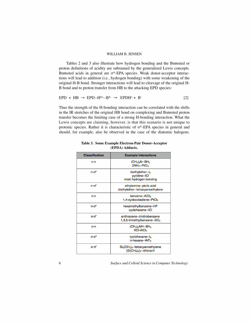
Tables 2 and 3 also illustrate how hydrogen bonding and the Brønsted or proton definitions of acidity are subsumed by the generalized Lewis concepts. Brønsted acids in general are σ*-EPA species. Weak donor-acceptor interac-tions will lead to addition (i.e., hydrogen bonding) with some weakening of the original H-B bond. Stronger interactions will lead to cleavage of the original H-B bond and to proton transfer from HB to the attacking EPD species:

EPD + HB → EPD--Hδ+--Bδ- → EPDH+ + B- [2]

Thus the strength of the H-bonding interaction can be correlated with the shifts in the IR stretches of the original HB bond on complexing and Brønsted proton transfer becomes the limiting case of a strong H-bonding interaction. What the Lewis concepts are claiming, however, is that this scenario is not unique to protonic species. Rather it is characteristic of σ*-EPA species in general and should, for example, also be observed in the case of the diatomic halogens.

WILLIAM B. JENSEN


Table 3. Some Example Electron-Pair Donor-Acceptor (EPDA) Adducts.

That this is indeed the case is shown in figure 3, which compares some typical donor-acceptor interactions for HCl and I2.10

These conclusions can also be reached by comparing more sophisticated theoretical quantum mechanical treatments of H-bonding, on the one hand, with those used for nonprotonic Lewis acid-base adducts or so-called charge-transfer adducts, on the other – a task performed by Ratajczak and Orville-Thomas in a 1980 review in which they wrote:

Thus finally one comes to the important conclusion that fundamentally there is no difference between “charge-transfer” and “hydrogen bond” interactions. Further, the hydrogen bond may be considered as a specific type of electron donor-acceptor interaction which is within the medium to strong range.11

Needless to say, consistent use of the generalized Lewis concepts not only pro-vides a common vocabulary and organizational framework for systematizing an enormous amount of previously unrelated chemistry (Table 4), it also eliminates



Figure 3. Parallels between the EPA propertries of I2 and HCl.

a great deal of redundant terminology in the process (Table 5). Many of the applications summarized in Table 4 are discussed in greater detail in reference 6.

2. Implications for Solubility Theory. Perhaps the simplest way to illustrate the implications of the Lewis concepts for surface chemistry is to first illustrate

WILLIAM B. JENSEN


Table 4. Chemical Phenomena Subsumed by the Generalized Lewis Concepts.

Table 5. Terminology Subsumed by the Generalized Lewis Concepts.

in some detail their impact on the theory of solubility, since an understanding of bulk phase compatibility is in many ways a necessary prerequisite to an un-derstanding of interfacial compatibility. From a thermodynamic point of view, predicting the solubility of a given species in a given solvent is quite straightforward – at least in principle. One simply writes down an expression for the partial free-energy of solution (ΔG2[sol]) for the solute (species 2):

ΔG2[sol] = ΔH2° - TΔS2° + RTlna2 [3]

makes use of the standard separation of the activity into a mole fraction contri-bution and an activity coefficient contribution:

RTlna2 = RTlnx2 + RTlnγ2 [4]

and uses standard thermodynamic relations to assess the relative contributions of the activity coefficient to the partial enthalpy (ΔH2[sol]) and entropy (ΔS2[sol]) of solution:

ΔH2[sol] = T2(∂(ΔG2[sol]/T)∂T) = ΔH2° - RT2(∂lnγ2/∂T) [5]

ΔS2[sol] = -(∂G2[sol]/∂T) = ΔS2° - Rlnx2 - Rlnγ2 - RT(∂lnγ2/∂T) [6]

The maximum solubility is then obtained by substituting either equation 4 or equations 5 and 6 back into equation 3 and applying the condition that ΔG2[sol] = 0 at equilibrium, which, upon solving for lnx2[eq] in terms of T, ΔH2°, ΔS2° and lnγ2[eq], gives the final result:

lnx2[eq] = -ΔH2°/RT + ΔS2°/R - lnγ2[eq] [7]

The only problem with this delightful scenario is what might be appropri-ately called “Dirac’s Catch 22.” This refers, of course, to Dirac’s famous – or rather infamous – claim that, with the advent of quantum mechanics, chemistry had been reduced to a branch of applied physics, since it is possible in principle to write down the correct form of the Schrödinger equation for virtually any chemical system of interest.12 The only difficulty – and this is the Catch 22 – is in solving the resulting differential equations. Similarly, in order to bridge the gap between principle and practice with equation 7, one must have a method of explicitly calculating ΔH2°, ΔS2° and lnγ2 or of relating them to other easily



measured properties of the system. The first significant step in translating solubility principle into solubility practice was taken nearly 70 years ago by Hildebrand13 and eventually evolved into what is now called regular solution theory.14, 15 Success was obtained in large part by restricting consideration to that class of solutions (called regular solutions) for which the activity coefficient contributions to the partial entropy of solution cancel:

Rlnγ2 = -RT(∂lnγ2/∂T) [8]

giving:

ΔS2[sol] = ΔS2° + ΔS2[mix] = ΔS2[tr] - Rlnx [9]

ΔH2[sol] = ΔH2° + ΔH2[mix] = ΔH2[tr] + RTlnγ2 [10]

Assuming the absence of specific compound formation between the solute and solvent, ΔS2° and ΔH2° become identical to the standard entropy and enthalpy of transition, ΔS2[tr] and ΔH2[tr], for the phase change required to bring the solute into the same phase as the solvent (equal to ΔS° and ΔH° of fusion or condensation for liquid solutions of solids and gases respectively). Likewise, ΔS2[mix] becomes identical to that of an ideal solution and all that is lacking is some way of evaluating ΔH2[mix] in terms of RTlnγ2. This remaining problem was eventually solved by recognizing that, for the vast majority of liquids forming regular solutions, the cohesive energy, as measured by the molar energy of vaporization, ΔU1[vap], is due almost totally to the operation of nondirectional, nonspecific dispersion forces:

ΔU1[vap] = ΔE1[dispersion] [11]

By defining a parameter δ1 (later called the solubility parameter of liquid 1) as equal to the square root of the liquid’s cohesive energy density:

δ1 = (ΔU1[vap]/V1)1/2 [12]

it is possible to approximate the rigorous theoretical expression for the change in the dispersion energy on mixing two liquids with the equation:

ΔH2[mix] = RTlnγ2 = V2φ12(δ1 - δ2)2 [13]

WILLIAM B. JENSEN


where V2 is the molar volume of the solute, φ1 is the volume fraction of the solvent (species 1) and δ1 and δ2 are the solubility parameters of the solvent and solute respectively. Thus equation 7 becomes:

lnx2[eq] = -ΔH2[tr]/RT + ΔS[tr]/R - V2φ12(δ1 - δ2)2 [14]

or, in the special case of liquid-liquid solutions, to which, for reasons of sim-plicity, we will restrict ourselves in what follows:

lnx2[eq] = -V2φ12(δ1 - δ2)2 [15]

Both of these equations correlate the degree of solubility with the square of the difference in the solubility parameters of the solute and solvent – a large differ-ence leading to small solubility and a small difference to high solubility. This result is, in effect, a quantification of the old adage that “like dissolves like,” where similarity of the cohesive energy densities as reflected in the solubility parameters is now our quantitative measure of “likeness.” Thus by using rigorous thermodynamics and a reasonable approximation for the partial enthalpy of mixing, Hildebrand and coworkers were able to suc-cessfully solve the problem of solubility for the special class of regular solu-tions. The only blemish to this approach is the fact that regular solutions and dispersion-only liquids form only a small subset of the solutions and solvents commonly employed by chemists. Consequently it is not surprising to discover that a good deal of effort has been expended in the last 30 years or so in at-tempts to extend Hildebrand’s work to other classes of liquids and solutions. Of these attempted extensions, many or which are summarized in Barton’s recent book,16 the most popular and ambitious is probably the extended solubil-ity approach of Hansen.17 Hansen’s model for the cohesive energy of a pure liquid allows for the operation of not only nonspecific dispersion interactions but for specific dipole (or polar) and hydrogen bonding interactions as well:

ΔU1[vap] = ΔE1[dispersion] + ΔE1[dipole] + ΔE1[H-bond] [16]

Each of these, in turn, is assigned a partial solubility parameter equal to the square root of the corresponding partial cohesive energy density:

Vδt2 = V(δd2 + δp2 + δh2) [17]

and Hansen has also suggested ways of independently approximating each



contribution.18 Finally, to complete the parallel with the more rigorous theory of regular solutions, but with little or no theoretical justification, an analogous three-term equation for ΔH2[mix] is used:

ΔH2[mix] = V2φ12[(δ1 - δ2)2d + (δ1 - δ2)2p + (δ1 - δ2)2h] [18]

containing the squared differences of each of the three types of partial solubil-ity parameters. Thus the criteria for high solubility is still one of “likeness,” though this measure is now a three-dimensional vector quantity rather than a one-dimensional scalar.19 Though the resulting model has not been very suc-cessful at a rigorous quantitative level, it has been quite useful in qualitatively extending the concepts of regular solution theory to a much broader range of solvents and solutions. But even at a qualitative level there are some serious problems connected with the use of equation 18, the most important of these being its inability to deal with exothermic heats of mixing and its incorrect modeling of H-bonding interactions. The importance of the first of these is illustrated in figure 4, which shows some typical experimental solubility curves for binary liquid systems. The H2O-phenol system on the left is the most common type, displaying in-creasing miscibility as the temperature increases, until it reaches a temperature of 65.85°C, called its critical solution temperature (CST), above which com-plete miscibility occurs.20 In contrast, the less common H2O-triethylamine sys-tem on the right shows exactly the opposite behavior, leading to increasing miscibility as the temperature is lowered and to a lower critical solution tem-perature of 18.5°C, below which complete miscibility occurs. Recognizing that

WILLIAM B. JENSEN


Figure 4. Some typical binary liquid-liquid phase diagrams.

the mole fraction of dissolved solute is essentially an equilibrium constant for the solution process, and applying Le Chatelier’s principle, leads at once to the conclusion that ΔH2[sol] for systems of the H2O-phenol type is endothermic in nature, whereas for systems of the H2O-triethylamine type it is exothermic. However, since equation 18 contains only the squares of the differences in δi it can only lead to positive or endothermic values of ΔH2[mix] and is conse-quently incapable of accounting for systems of the H2O-Et3N variety. This defect is closely related to the second problem, namely the incorrect modeling of the H-bonding interactions. Use of the difference term (δ1 - δ2)2h for H-bonding is equivalent to the claim that, like dispersion interactions, effec-tive solute-solvent H-bonding depends on some likeness or similarity of the two liquids, when in reality it depends on the complementary matching of the two liquids as illustrated in Table 6. As a consequence, this term leads to the incorrect inference that the strongest H-bonding interaction between a solute and solvent will occur when the pure liquids themselves are strongly self-associated by H-bonding, though in fact the opposite is frequently true. Indeed, this is well illustrated by the binary systems in figure 4, where phenol and wa-ter, both of which are strongly self-associated by H-bonding, give rise to an unfavorable enthalpy of solution, whereas triethylamine, which exhibits little self-association due to H-bonding but is a good H-bonding acceptor species, gives a favorable enthalpy of solution with water. In short, the ability to act as a strong H-bonding acceptor species in no way implies the necessary existence of the complementary ability to act as a strong H-bonding donor and vice versa, though most species are amphoteric to some degree and should be character-ized with respect to both properties. The simplest way of achieving this and of incorporating the inherently complementary nature of H-bonding into the expression for ΔH2[mix] is to make -ΔE1[H-bond] for a pure liquid the product of two inherently positive numbers, one of which characterizes the liquid’s proton donor ability (PD1) in a



Table 6. The Failure of Equation 18 to Indicate the Complementary Nature of H-Bonding Interactions.

H-bonding interaction, and the other its proton acceptor ability (PAl):

-ΔE1[H-bond] = PD1PA1 [19]

Using a similar expression for H-bonding between different species as well, the change in the H-bonding energy on mixing two liquids can then be approxi-mated using the simplified one-dimensional model in Table 7. Summing the interactions in the table gives:

ΔEmix[H-bond] = PD1PA1 + PD2PA2 - PD1PA2 - PD2PA1 [20]

and application of some high school algebra leads to the final result:

ΔEmix[H-bond] = (PD1 - PD2)(PA1 - PA2) [21]

first suggested by Small over 30 years ago.21 As can be seen, equation 21 not only incorporates complementarity by predicting that the most favorable inter-

action will involve a high PA/low PD liquid and a low PA/high PD liquid, but also resolves the first problem, since the product of the two differences may either be positive (endothermic) or negative (exothermic) in sign. The first important attempt to use a Small-like equation appears to have been that of Keller et al in 1970,22 who used a set of corresponding Brønsted base, δb (equivalent to PA) and Brønsted acid, δa (equivalent to PD) solubility parameters defined by the equation:

-ΔE1[H-bond] = 2Vδaδb [22]

WILLIAM B. JENSEN


Table 7. A Simple One-Dimensional Model for the Mixing of Two Liquids.

and a corresponding expression for ΔH2[mix]:

-ΔH2[mix] = V2φ12[(δ1 - δ2)2d + (δ1 - δ2)2p + 2(δ1 - δ2)a(δ1 - δ2)b] [23] Although this approach incorporates both complementarity and the possi-bility of exothermic interactions, its use of a composition dependent H-bonding term (via the V2φ12 multiplier) and a set of corresponding Brønsted solubility parameters is more open to question. At a naive level, the use of a composition-dependent enthalpy of mixing term for the dispersion-only interactions in the original form of regular solution theory stems from the fact that dispersion in-teractions are nonspecific. Since the average composition of the fluctuating coordination sphere about a given molecule will vary as the composition of the bulk solution varies, so presumably will the average value or the enthalpy. In contrast, in the case of H-bonding we are dealing with a specific interaction and with adducts of fixed composition. Consequently the enthalpy of this interac-tion should ideally be invariant to the composition of the bulk solution and, to a first approximation, be determined by a fixed number depending only on the chemical natures of the solute and solvent, as in Small’s original suggestion. At a more practical level, difficulties in obtaining a sufficiently broad range of δb and δa parameters for common solvents, as well as problems in obtaining chemically reasonable self-consistency in the values of δa, appear to have pre-vented extensive use of equation 23, though Martin et al have recently applied it to problems of drug solubility.23 Having eliminated two of the more serious problems in the Hansen model, what remains to be done? The answer, of course, lies in the further realization that H-bonding is not really a particular kind of intermolecular “force,” like a dipole or dispersion force, but rather, as emphasized earlier, an example (albeit, a very important one) of a generalized electron-pair donor-acceptor or Lewis acid-base interaction. Consequently the H-bonding term in equation 23 should be replaced with a generalized EPD-EPA term. Since these interactions are spe-cific and yield adducts (however fleeting) of fixed composition, they should also be modeled along the lines of Small’s complementarity equation, with the PA parameter now being subsumed within a more generalized electron-pair donor number (DN) and the PD parameter within a more generalized electron-pair acceptor number (AN), giving:

ΔHmix[DA] = k(AN1 - AN2)(DN1 - DN2) [24]

where k is a scaling constant of some sort.



As will be seen later, an examination of both theoretical and empirical measures of Lewis acid-base strengths will suggest yet a third modification of equation 23, as they both indicate that most specific electrostatic or polar inter-actions are already included within conventional measures of electron-pair donor and acceptor strengths, making the separate polar term in the equation potentially redundant. In short, a consideration of solubility phenomena from the standpoint of the Lewis concepts suggests that the simplest possible chemi-cal models for the cohesive energy of a pure liquid and for the enthalpy of mix-ing for a binary liquid-liquid solution are two-term equations of the forms:

ΔU1[vap] = ΔE1[dispersion] + ΔE1[DA] = V1δ2d + kAN1DN1 [25]

ΔH2[mix] = V2φ12(δ1 - δ2)2d + k(AN1 - AN2)(DN1 - DN2) [26]

3. Implications for Surface Chemistry. One reason for reviewing the devel-opment of solubility theory in such detail is that the empirical treatment of sur-face phenomena, and especially that dealing with the work of adhesion, has followed a virtually identical course of development. On the basis of the ap-proximations used for dispersion-only liquids in the theory of regular solutions, it is reasonable to expect a relationship between the work of adhesion (W12[adh]) of two phases and their surface tensions (γ) of the form:

W12[adh] = 2φ(γ1γ2)1/2 [27]

where φ is a constant originally thought to depend on the molecular volumes and, indeed, such a relationship was experimentally confirmed by Girifalco and Good in 1957.24 In an effort to extend equation 27 to other classes of liquids, Fowkes sug-gested in 196225, 26 that both the work of adhesion and surface tensions could be decomposed into dispersion, dipole and hydrogen bonding components in a manner similar to Hansen’s later decomposition of the solubility parameter:

W12[adh] = W12[disp] + W12[polar] + W12[H-bond] [28]

γt = γd + γp + γh [29]

and that a relationship similar to equation 27 could be used to reasonably ap-proximate the dispersion component and, to a less rigorous degree, the polar component as well:

WILLIAM B. JENSEN


W12[adh] = 2(γ1γ2)d1/2 + 2(γ1γ2)p1/2 + W12[H-bond] [30]

Later writers attempted to also apply the geometric mean approximation to the hydrogen bonding component, though, as with the enthalpy of solution, it is incorrect to use an approximation suitable only for nonspecific interactions to model a specific complementary interaction. In 1978 Fowkes and Mostafa27 proposed a modified expression for W12[adh] in which the hydrogen bonding component was incorporated within a general-ized donor-acceptor term:

W12[adh] = 2(γ1γ2)d1/2 + 2(γ1γ2)p1/2 + tkΔH12[DA] [31]

where k is a scaling constant that converts enthalpy per mole into free energy per unit area and t is the number of moles of donor-acceptor interactions per unit area. However, use of this model quickly showed that the polar term was redundant and that a two-term equation, paralleling equations 25 and 26 could be used instead:26

W12[adh] = W12[disp] + W12[DA] [32]

Use of Fowkes’ expression for the dispersion component along with a gen-eralized Small equation for the donor-acceptor component then gives:

W12[adh] = 2(γ1γ2)d1/2 +k[AN1(xDN2 - mDN1) + AN2(yDN1 - nDN2)] [33]

where k is the scaling constant, x is the moles of donor sites per unit area at the surface of phase 2 interacting with phase 1, y is the moles of donor sites per unit area at the surface of phase 1 interacting with phase 2, and m and n repre-sent the moles of additional sites for self-association created in phases 1 and 2 upon their separation and are related to the changes in their surface areas upon separation. In the case of gases or solids m and n can be assumed to be vanish-ingly small, but they may be significant in the case of liquids. Using established relations between WI2[adh] and surface tensions, it is also possible to write down similar expressions for the dependency of spreading coefficients and con-tact angles on the donor-acceptor properties of the interacting phases. A more complex situation is the adsorption on a solid of a component from a solution, since it involves desolvation of the component as well as possible competition between the adsorbate and the solvent for the surface sites of the solid. A generalized Small equation for approximating the donor-acceptor con-



tribution to the enthalpy of adsorption for this situation would be of the form:

ΔHabs[DA] = k[-xANsDNa - yANaDNs - (tA - x)ANsDNl - (tD - y)ANlDNs + .... .... (x + y)(ANaDNl + ANlDNa) + (tA + tD -2x - 2y)ANlDNl] [34]

where the subscripts s, a, and l stand for the solid surface, dissolved adsorbate, and liquid solvent respectively, tA and tD for the total moles of acceptor and donor sites per unit area on the surface, and x and y for the moles of these sites occupied by the adsorbate. The first two terms in this equation represent the adsorption of the dissolved adsorbate species, the second two terms the com-petitive adsorption of the solvent, the third term the desolvation of the adsor-bate, and the fourth term the changes in solvent self-association due either to desolvation of the adsorbate or removal of solvent molecules for adsorption from the bulk solvent. Actual quantitative use of either equation 33 or 34 is severely hampered by the necessity of not only having to know the donor and acceptor numbers of all of the species but the number of moles per unit area of each kind of interaction site.29 Nevertheless, as will be seen, a knowledge of just the donor and acceptor numbers alone is still sufficient to qualitatively predict conditions that will maximize or minimize the occupation of certain kinds of sites and with them trends in the degrees of adsorption, contact angles, work of adhesion, and spreading coefficients as a function of the Lewis acid-base properties of the interacting phases.

4. Implications for Colloid Chemistry. As noted in Table 5, the phenomenon of ionic dissociation is one of the topics subsumed by the generalized Lewis concepts. If a species XY is dissolved in an EPD solvent, the solvent will tend to interact with the more electropositive or acidic site on the molecule, leading to a heterolytic weakening of the original X-Y bond and to incipient ion formation:

EPD + XY → EPD--Xδ+--Yδ- [35]

If the solvent is a sufficiently strong donor, this process will proceed to comple-tion, giving rise to a contact ion pair consisting of a solvated cation and a naked anion, and these may, in turn, dissociate into independent ions capable of con-tributing to the solution’s conductivity provided that the solvent’s dielectric constant is high enough to separate them:30, 31

EPD--Xδ+--Yδ- → EPD--X+ + Y- [36]

WILLIAM B. JENSEN


The mechanism outlined in equation 2 for hydrogen bonding and proton trans-fer is a special case of this process, where X+ represents the proton and Y- the conjugate Brønsted base. Within the context of the Lewis concepts, however, all possible cationic species X+ are inherently acidic. If a strong EPA solvent is used instead, the complementary process will occur, giving rise to a solvated anion and a naked cation:

X-Y + EPA → Xδ+--Yδ---EPA → X+ + Y-EPA- [37]

Obviously a liquid which is both a strong EPD and a strong EPA species (i.e., strongly amphoteric), and which also has a high dielectric constant, can com-bine both of these processes and will function as a strongly ionizing solvent – a set of properties corresponding almost exactly to those of water. There is no reason, however, that X-Y must be a dissolved molecular fragment of some sort. It could just as well represent a molecule or a pair of adjacent atoms on the surface of an immiscible phase in contact with the liquid. In this case process 36 would lead to the transfer of X+ from the surface to the liquid, leaving the former with a net negative charge and the latter with a net positive charge. Likewise, process 37 would lead to the reverse transfer and to an opposite separation of charges between the surface and the liquid. A similar reversal could also occur for process 36 if the surface should prove to be a stronger donor than the liquid, as this would reverse their roles and X-Y In equation 36 would then represent the liquid and EPD the surface of the other phase. Likewise, a similar charge reversal could occur for process 37 if the surface proved to be a stronger EPA agent than the liquid. Combining these various possibilities, one would expect to observe a sign reversal in the surface charge if a solid is immersed in a series of liquids of relatively constant EPA strength but gradually increasing EPD strength, the surface being positive when in contact with liquids that are weaker donors than the surface and negative when in contact with those that are stronger donors. Similarly, immersing a solid in a series of liquids of relatively constant EPD but gradually increasing EPA strength should give a negative surface charge for those that are weaker EPA agents than the surface and a positive charge for those that are stronger. What is being discussed here, of course, is really a gen-eralization of a molecular mechanism for generating zeta potentials, first sug-gested by Fowkes32 nearly 20 years ago for the more limited case of proton transfer, and the importance of such potentials in stabilizing colloidal disper-sions, ranging from paints33 and inks to fillers in polymers, need hardly be stressed.



Quantifying these considerations is, however, more difficult as most spe-cies are to some extent amphoteric and their EPA and EPD properties tend to work in opposite directions as far as the sign and magnitude of the zeta poten-tial are concerned. Perhaps the simplest approach to this problem would be to use an empirical linear correlation similar to that proposed by Koppel and Pal’m in 1971 to analyze the solvent dependency of various physico-chemical properties:34

P = P0 + αDN + βAN + ξδd [38]

where P is the value of the property in the solvent of interest, P0 is the value of the property in some reference state (preferably, but not necessarily, the gas phase or some inert solvent), α describes the sensitivity of the property to sol-vent basicity, β its sensitivity to solvent acidity, ξ its sensitivity to nonspecific dispersion forces, and the property in question may be a spectral transition, the logarithm of a rate constant or an equilibrium constant, a reaction enthalpy, an NMR shift, or, in our case, the zeta potential of a colloidal particle. Generally if the EPA-EPD character of the solvent is significant, it tends to swamp the last term and a simpler three-term correlation proposed by Krygowskl and Fawcett35-37 in 1974 can be used instead:

P = P0 + αDN + βAN [39]

5. Quantitative Measures of Lewis Acid-Base Strengths. In order to im-plement equations 25-26, 33-34, and 38-39 one requires, of course, some method of assigning DN and AN values to each species. This can be done by designing a probe which is selectively sensitive to either Lewis acidity or ba-sicity alone and by applying equation 39 in reverse:

DN = (P - P0)/α (base-only sensitive probe, β = 0) [40]

AN = (P - P0)/β (acid-only sensitive probe, α = 0) [41]

Assigning arbitrary values to α, β and P0 and monitoring the changes in the selected properties P as a function of the species interacting with the probes, then serves to define DN and AN scales for the interacting species. Usually the probes are single chemical species whose properties are altered via their selec-tive interaction with either the EPD or EPA functions of the species being char-acterized – in which case the probes are called reference acids and bases re-

WILLIAM B. JENSEN


spectively. In principle, however, this need not necessarily be the case and the probes could, for example, be model displacement or elimination reactions whose rate or equilibrium constants are selectively sensitive to the Lewis acid-ity or basicity of the surrounding solvent. As originally defined by Gutmann and coworkers31, 36 the DN is based on -ΔHrx of the standard EPA probe antimony(V) chloride with the species of in-terest in a dilute 1,2 dichloroethane solution:

D: + SbCl5 → D-SbCl5 DN = -ΔHrx [42]

where P = -ΔHrx, P0 = 0, α = 1 in equation 40. The AN, on the other hand, is based on the volume corrected difference at infinite dilution in the 31P NMR shift induced in the standard EPD probe triethylphosphine oxide (Et3P-O) by the species of interest and that induced by n-hexane, (HX) scaled, in turn, rela-tive to the shift induced by SbCl5 in a dilute 1,2 dichloroethane solution: 31, 39

Et3P-O + A → Et3Pδ+-Oδ---A [43]

where P = 100(δ∞[A] - δ∞[HX])corr/(δ∞[SbCl5] - δ∞[HX])corr, P0 = 0, and β = 1 in equation 41. The factor of 100 essentially converts the AN of a species into a percentage of that shown by SbCl5. Consequently calculation of ΔHrx[DA] for an interaction via equation 19 requires a reconversion to the fraction, giving:

-ΔHrx[DA] = ANADND/100 [44]

DN values have been experimentally determined for about 53 liquids and AN values for about 34. Regrettably, however, these two sets of liquids are not identical, and their overlap allows for the complete characterization of the EPA-EPD properties of only about 25 different species. As shown in figure 5, these can, in turn, be qualitatively classified as being primarily donor solvents (low AN/high DN), acceptor solvents (high AN/low DN), amphoteric solvents (high AN/high DN) and nonspecific or dispersion solvents (low AN/low DN).40, 41 Luckily there are measurements of many other probes and properties available which are also selectively sensitive to either Lewis acidity or basicity. Some examples are listed in Tables 8 and 9 and many additional correlations can be found in either the review of Griffiths and Pugh42 or in the book43 and reviews44-46 of Reichardt. Again, by use of equation 39 and the resulting linear correlations, these are easily converted into equivalent DN and AN values:



DN = P/α - P0/α (base sensitive) [45]

AN = P/β - P0/β (acid sensitive) [46]

y = ax + b (in general) [47]

and in cases where either the DN or the AN alone is known, a property sensitive to both can be used to find the missing member of the pair:

DN = (P - P0 - βDN)/α [48]

AN = (P - P0 - αDN)/β [49]

By use of such linear relations for the properties summarized in Table 10, our group has recently compiled a list of best averaged DN and AN values for about 150 different solvents, including water, allowing for a much more extensive

WILLIAM B. JENSEN


Figure 5. A plot of the donor number (DN) versus the acceptor number (AN) for a vari-ety of solvents. Key: HX = n-hexane, Et2O = diethylether, THF = tetrahydrofuran, BZ = benzene, HMPA = hexamethylphosphoramide, DO = dioxane, AC = acetone, NMP = N-methyl-2-pyrrolidinone, DMA = N,N-dimethylacetamide, Py = pyridine, NB = nitro-benzene, BN = benzonitrile, DMF = dimethylformamide, DEC = dichloroethylene car-bonate, PC = propylene carbonate, AN = acetonitrile, FA = formamide, DMSO = di-methylsulfoxide, DM = dichloromethane, NM = nitromethane, EtOH = ethanol, MeOH = methanol, AcOH = acetic acid.



Table 8. Other Properties Selectively Sensitive to Lewis Basicity

Table 9. Other Properties Selectively Sensitive to Lewis Acidity.

semi-quantitative application of the Lewis concepts than previously. An example of this in the case of solubility is shown in figure 6, which shows a qualitative sorting map,47, 48 based on equation 26, for the miscibility of 72 binary liquid mixtures involving 21 different liquids at 25°C. As expected, the miscible systems tend to cluster in the lower left hand corner, reflecting both favorable donor-acceptor and dispersion interactions upon mixing, whereas the immiscible systems show the opposite behavior. Once established, this map can be used, via interpolation, to predict the miscibility of other systems for which the DN, AN and δd parameters of the component liquids are known.49 An example involving equation 34 and adsorption from solution is shown in figure 7. This is based on the data of Fowkes and Mostafa27 for the adsorp-tion of a basic adsorbate (poly(methyl methacrylate) or PMMA) onto an acidic

WILLIAM B. JENSEN


Table 10. Some Linear Relations for Determining Additional DN ad AN Values.

Figure 6. Sorting map for miscible (black circles) and immiscible (open circles) binary liquid mixtures based on the application of equation 26.

surface (SiO2 – acidity due to surface -OH groups) from solvents with varying EPA and EPD properties. Assuming that ANa = 0 and DNs = 0, equation 34 re-duces to:

-xANsDNa - (tA - x)ANsDNl + (x + y)ANlDNa + (tA + tB - 2x - 2y)ANlDNl [50]

Use of solvents of approximately constant AN but variable DN makes the sec-ond term in equation 50 the controlling factor in optimizing ΔHads[DA] and this, in turn, leads to the prediction that x, the number of surface sites occupied by the PMMA, will decrease as the DN of the solvent increases. In other words, as the EPD properties of the solvent increase it will successfully compete with the basic PMMA for the acidic surface sites of the SiO2. Conversely, use of solvents of relatively constant DN but variable AN will make the third term the controlling factor in optimizing ΔHads[DA], again leading to a decrease in x as the acidity of the solvent increases – this time due to the competitive solvation of the basic PMMA by the solvent. As figure 7 shows, these predictions are confirmed by experiment. A reversed system consisting of adsorption of an acidic adsorbate (post-chlorinated poly(vinylchlorlde) or Cl-PVC) onto a basic surface (CaCO3) from solvents of varying EPD-EPA properties was also studied by Fowkes and Mo-stafa. Again, by assuming that DNa = 0 and ANs = 0, a limiting case of equation 34 can be used which predicts that solvents of increasing AN values will de-



Figure 7. Adsorption of basic PMMA onto an acid SiO2 surface from solvents of variable basicity (left) and variable acidity (right) as given in reference 40.

crease adsorption of Cl-PVC due to competition for the basic surface sites and solvents of increasing DN values will decrease it due to more effective solva-tion of the adsorbate species (figure 8). Williams50 has explored the development of contact charges between a flowing liquid and a solid surface as a function of the liquid’s DN. Though the results (figure 9) were originally rationalized using an electron transfer model, they are consistent with the ion transfer model discussed earlier and show that liquids of low donicity acquire a negative charge due to transfer of X+ to the surface of the solid, whereas liquids of high donicity acquire a positive charge

WILLIAM B. JENSEN


Figure 8. Adsorption of acidic Cl-PVC onto a basic Ca(CO3) surface from solvents of variable basicity (left) and variable acidity (right) as given in reference 40.

Figure 9. Charge acquired by a flowing liquid in contact with various solid surfaces. Key: TEA = triethyl amine, DMA = N, N-dimethylacetamide, EA = ethyl acetate, AA = acetic anhydride, DCE = 1, 2-dichloroethane, TEF = teflon, ACR = methylmethacrylate, Ni = nickel, PE =polyethylene, PHEN = phenolic polymer. Shaded areas indicate approximate donici-ties of the surfaces (from reference 50).

due to transfer of X+ in the opposite direction. This cross-over point is pre-sumably an indication of the DN value of the surface. Labib and Williams51 have also extended this work to the measurement of the zeta potentials of the suspended particles of a variety of inorganic solids as a function of the donicity of the surrounding liquid, again obtaining results (Table 11) largely in keeping with the ion transfer model, though some inconsistencies were observed. How-ever, since not all of the liquids used had similar AN values and, as pointed out earlier, variations in this parameter can have an opposite effect on the zeta po-tential, these data should really be reexamined from the standpoint of equations 38 and 39. Use of equation 44 and the other Small-like expressions for calculating the enthalpies of EPA-EPD interactions is equivalent to the assumption that a sin-gle universal scale or order of Lewis acid-base strengths exists. Experimental evidence, however, shows that this is not rigorously true. For example, the EPD species in Table 12 show a different order of base strengths depending on whether they are measured relative to their interaction with the Lewis acid Me3Ga or the Lewis acid I2.52 Even more striking examples are found for ionic Lewis acids and bases. Thus in aqueous solution the halide ions give the EPD order F- >> Cl- > Br- > I- when measured relative to the Lewis acid H+ but the



Table 11. Zeta Potentials of Various Solids as a Function of the Donicity of the Surrounding Liquid.

a Abbreviations are the same as those used in earlier tables.

reverse order when measured relative to the Lewis acid Hg2+. The qualitative interpretation of these inversions is the basis of the so-called hard and soft acid-base (HSAB) principle53 and their quantitative treatment is to be found in the E&C equation of Drago and coworkers:54, 55

-ΔHAB = EAEB + CACB [51]

where the E parameters measure a species’ susceptibility to electrostatic or ionic interactions and the C parameters its susceptibility to covalent or orbital perturbation interactions. Since, in principle, these two factors can vary inde-pendently of one another, equation 51 is capable of yielding a different order of ΔHAB values for a series of bases when the reference acid is changed and vice versa. Like the Small approach, the E&C equation uses two parameters to charac-terize each species (E and C versus AN and DN) and four to calculate each in-teraction. But unlike the Small approach, it does not recognize the inherently amphoteric nature of most species and treats each of them as being either ex-clusively an acid or a base. Consequently the approach cannot be used to de-termine the contribution of EPA-EPD interactions to the self-association of a species. Thus, in choosing a quantitative approach to Lewis acid-base phenom-ena, we must decide between a method that treats amphoteric interactions but naively assumes universal orders of strength, on the one hand, and a method which deals with variations in orders of strength but ignores amphoteric inter-actions, on the other. Which is the correct choice? As might be expected with such simple models, the answer is that neither method is completely correct and the choice largely depends on the dictates of the systems one is dealing with. For example, a crude quantum mechanical treatment of EPA-EPD inter-actions by Klopman and Hudson,56,57 using second-order perturbation theory, shows that a minimum of three terms is necessary to approximately describe the interaction:

WILLIAM B. JENSEN


Table 12. Gas-phase Basicities as a Function of the Reference Lewis Acid.

ΔEAD = Σrs(QrQs/Rrs) + ΣoccΣunocc2(Σrscrmcsnβrs)2/(Em - En) + ... ... ΣoccΣunocc2(Σrscrmcsnβrs)2/(En - Em) [52]

The first of these represents a classical electrostatic or charge-control term, whereas the second and third represent covalent or orbital control terms, one in which species D acts as the EPD agent and the other in which species A does. The importance of these orbital control-terms depends largely on the size of their denominators and these, in turn, reflect the difference in the energies of the donor and acceptor orbitals and especially those of the HOMOs and LUMOs. The smaller these energy differences, the larger the respective orbital-controlled interactions and vice versa. It is reasonable to view the ANADND and ANDDNA terms in the Small equation as empirical approximations of these orbital control-terms and, indeed, Paoloni et al58 have actually established approximate correlations between the DN and AN values of a species and the energies of the species’ HOMO and LUMO orbitals. Although the present writer is not aware that any similar correlations have been established for the E&C equation, it is still not unreasonable to view the EAEB term as an empirical ap-proximation of the charge-control term and the CACB term as an approximation of the first of the two orbital-control terms. In short, the Small approach views the independent variation of the last two terms in equation 52 as being the most important, whereas the E&C equation views the independent variation of the first two terms as being the most important. Actually the relative importance of the terms varies with the systems being studied. The donor and acceptor sites on a species are usually located on differ-ent atoms and in dilute systems, and particularly in the gas phase, the species, for stereochemical reasons, will probably select one of the two modes in its interactions. In condensed systems, however, where the species is surrounded on all sides, It is likely to exercise both modes of interaction simultaneously, though usually with two different partners. Thus amphoteric properties become decidedly more important in the liquid and solid phases. Likewise, if one is dealing with systems in which the only donor atoms are N and O and most of the acceptor sites are H-bonding, then inversions in strength due to variations in hardness and softness are at a minimum, in contrast to systems also having S or P donor sites, for example, or Hg2+ or I2 as acceptors. These conclusions are summarized In Table 13 and it is on this basis – namely the fact that in the sys-tems which we have been describing we are working with relatively hard spe-cies in the liquid and solid states and with processes in which competition with the self-association of the pure components is important, that we have chosen to work with the Small equation and with the donor and acceptor number



scales. Fowkes, on the other hand, has successfully applied the E&C equation to some of the same systems.27-28, 59 The ideal solution, of course, would be to have an E and C parameter for both the donor and acceptor ability of each spe-cies, though this would result in a total of four parameters per species and eight per interaction, and perhaps rather stretches the usefulness of an empirical ap-proach to Lewis acid-base interactions.

6. Conclusions. As the above examples illustrate, the Lewis concepts have an enormous potential for clarifying many phenomena of interest to chemists working in the fields of surface chemistry, colloid chemistry, and adhesion and, with the very notable exception of the pioneering work of Fowkes and his coworkers,27-28, 59 this potential is still largely untapped. At present most of this work is at a semi-quantitative empirical level. But even at a purely qualitative level the Lewis concepts are of value, if for no other reason than the fact that they refocus thinking on the complementary matching of properties for favor-able interactions rather than on the similarity matching of properties which still pervades many of these areas as a result of an inappropriate extension of the dispersion-only arguments used in the original theory of regular solutions.

7. References

1. G. N. Lewis, Valence and the Structure of Atoms and Molecules, The Chemical Catalog Company: New York, NY, 1923, pp. 141-142. 2. G. N. Lewis, J. Franklin Inst., 1938, 226, 293. 3. K-H Sun, A. Silverman, J. Am. Ceram. Soc.,1945, 28, 8. 4. K-H Sun, Glass Ind., 1948, 29, 73. 5. R. S. Mulliken, W. B. Person, Molecular Complexes: A Lecture and Reprint Volume, Wiley-Interscience: New York, NY, 1969. 6. W. B. Jensen, The Lewis Acid-Base Concepts: An Overview, Wiley-Interscience:

WILLIAM B. JENSEN


Table 13. A Comparison of the DN/AN Approach and the E&C Equation.

New York, NY, 1980. 7. H. Burgi, Angew. Chem. Int. Ed. Eng., 1975, 114, 460. 8. J. D. Dunitz, X-Ray Analysis and the Structure of Organic Molecules, Cornell University Press: Ithaca, NY, 1979. 9. V. F. Traven, R. West, J. Am. Chem. Soc., 1973, 95, 6824. 10. H. C. Brown, J. Phys. Chem., 1952, 56, 821. 11. H. Ratajczak, W. J. Orville-Thomas, Molecular Interactions, Vol. I, Wiley-Interscience: New York, NY, 1980, Chap. 1. 12. P. Dirac, Proc. Royal Soc. London, Ser. A., 1929, 123, 714. 13. J. H. Hildebrand, J. Am. Chem. Soc., 1916, 38, 1452. 14. J. H. Hildebrand, R. L. Scott, The Solubility of Nonelectrolytes, Reinhold: New York, NY, 1950. 15. J. H. Hildebrand, M. M. Prausnitz, R. L. Scott, Regular and Related Solutions, Van Nostrand-Reinhold: New York, NY, 1970. 16. A. F. M. Barton, Handbook of Solubility Parameters and Other Cohesion Parameters, CRC Press: Boca Raton, FL, 1983. 17. C. M. Hansen, Ind. Eng. Chem. Prod. Res. Dev., 1969, 8, 2. 18. C. M. Hansen, A. Beerbower in A. Standen, Ed., Kirk-Othmer Encyclopedia of Chemical Technology, Suppl. Vol., 2nd ed., Wiley-Interscience: New York, NY, 1971, p. 889. 19. D. L. Wernick, Ind. Eng. Chem. Prod. Res. Dev., 1984, 23, 240. 20. A. W. Francis, Critical Solution Temperatures, Adv. Chem. Series No. 31, American Chemical Society: Washington, D.C., 1961. 21. P. A. Small, J. Appl. Chem., 1953, 3, 71. 22. R. A. Keller, B. L. Karger, L. R. Synder in R. Stock, S. F. Perry, Eds., Gas Chromatography 1970, Institute of Petroleum Research: London, 1971, p. 125. The original equation also contained an induced dipole term, though the work of Martin et al23 suggests that it can be neglected. 23. A. Beerbower, P. L. Wu, A. Martin, J. Pharm. Sci., 1984, 73, 179, 188. 24. L. A. Girifalco, R. J. Good, J. Phys. Chem., 1957, 61, 904. 25. F. M. Fowkes, J. Phys. Chem., 1962, 66, 382. 26. F. M. Fowkes, Ind. Eng. Chem., 1964, 56(12), 40. 27. F. M. Fowkes, M. A. Mostafa, Ind. Eng. Chem. Prod. Res. Dev., 1978, 17, 3. 28. F. M. Fowkes in K. L. Mittal, Ed., Physicochemical Aspects of Polymer Sur-faces, Vol. 2, Plenum: New York, NY, 1983, p. 583. 29. K. Tanabe, Solid Acids and Bases, Academic Press: New York, NY, 1970. 30. V. Gutmann, Angew. Chem. Int. Ed. Eng., 1970, 9, 843. 31. V. Gutmann, The Donor-Acceptor Approach to Molecular Interactions, Plenum: New York, NY, 1978. 32. F. M. Fowkes, Disc. Faraday Soc., 1966, 42, 246.



33. P. Sørensen, J. Paint Tech., 47, 31 (1975). 34. I. A Koppel, V. A. Pal’m in J. Shorter, Ed., Advances in Linear Free-Energy Relationships, Plenum: New York, NY, 1972, Chap. 5. The original equation also con-tained a dipole term. We have also substituted a more logical choice of symbols. 35. T. M. Krygowski, W. R. Fawcett, J. Am. Chem. Soc., 1975, 97, 2143. 36. W. R. Fawcett, T. M. Krygowski, Aust. J. Chem., 1975, 28, 2115. 37. W. R. Fawcett, T. M. Krygowski, Can. J. Chem., 1976, 54, 3283. 38. V. Gutmann, E. Wychera, Inorg. Nucl. Chem. Lett., 1966, 2, 257. 39. U. Mayer, V. Gutmann, W. Gerger, Monatsh. Chem., 1975, 106, 1235. 40. W. B. Jensen, Rubber Chem. Techn., 1982, 55, 881. 41. W. B. Jensen, Chemtech., 1982, 12, 755. 42. T. R. Griffiths, D. C. Pugh, Coord. Chem. Rev., 1979, 29, 129. 43. C. Reichardt, Solvent Effects in Organic Chemistry, Verlag Chemie: New York, NY, 1979. 44. C. Reichardt, Angew. Chem. Int. Ed. Engl., 1979, 18, 98. 45. C. Reichardt, Pure Appl. Chem., 1982, 54, 1867. 46. C. Reichardt in H. Ratajczak, W. J. Orville-Thomas, Eds., Molecular Interac-tions, Vol. 3, Wiley-Interscience: New York, NY, 1982, Chap. 5. 47. For background on the philosophy of sorting maps, see A. Beerbower, W. B. Jensen, Inorg. Chem. Acta, 1983, 75, 193 and Wold.48

48. S. Wold, M. Sjöström in R. F. Gould, Ed., Chemometrics: Theory and Applicat-lons, ACS Symposium Series No. 52, American Chemical Society: Washington, D.C., 1977, Chap. 12. 49. W. B. Jensen in D. Hertz, Ed., Proceedings Symposium on Migration of Gases, Liquids, and Solids in Elastomers, 126th National Meeting of the Rubber Division, American Chemical Society: Denver, CO, 1984. 50. R. Williams, J. Colloid Interface. Sci., 1982, 88, 530. 51. M. E. Labib, R. Williams, J. Colloid Interface. Sci., 1984, 97, 356. 52. K. F. Purcell, J. C. Kotz, Inorganic Chemistry, Saunders: Philadelphia, PA, 1977, p. 218. 53. R. G. Pearson, Ed., Hard and Soft Acids and Bases, Dowden, Hutchinson and Ross: Stroudsburg, PA, 1973. 54. R. S. Drago, B. Wayland, J. Am. Chem. Soc., 1965, 87, 3571. 55. R. S. Drago, Struct. Bonding (Berlin), 1973, 15, 73. 56. R. F. Hudson, G. Klopman, Theor. Chim. Acta, 1967, 8, 165. 57. G. Klopman, Ed., Reactivity and Reaction Paths, Wiley-Interscience: New York, NY, 1974. 58. A. Sabatino, G. La Manna, L. Paoloni, J. Phys. Chem., 1980, 84, 2641.

WILLIAM B. JENSEN


59. F. M. Fowkes, D. O. Tischler, J. A. Wolfe, L. A. Lannigan, C. M. Ademu-John, M. J. Halliwell, J. Polymer Sci., 1984, 22, 547. 60. P. Maria, J. Gal, J. Phys. Chem., 1985, 89, 1296. 61. R. Schmid, J. Solution Chem., 1983, 12, 135.

8. Publication History. Originally published in K. L. Mittal, Ed., Surface and Colloid Science in Computer Technology, Plenum: New York, NY, 1987, pp. 27-59.



the relevance of lewis acid-base chemistry to surface interactions

Documents