the relationship between abnormal inventory growth...
TRANSCRIPT

MANUFACTURING & SERVICEOPERATIONS MANAGEMENT
Articles in Advance, pp. 1–18ISSN 1523-4614 (print) � ISSN 1526-5498 (online) http://dx.doi.org/10.1287/msom.1120.0389
© 2012 INFORMS
The Relationship Between Abnormal InventoryGrowth and Future Earnings for U.S. Public Retailers
Saravanan KesavanKenan-Flagler Business School, University of North Carolina at Chapel Hill, Chapel Hill, North Carolina 27599,
Vidya ManiSmeal College of Business, Pennsylvania State University, University Park, Pennsylvania 16802,
In this paper we examine the relationship between inventory levels and one-year-ahead earnings of retailersusing publicly available financial data. We use benchmarking metrics obtained from operations management
literature to demonstrate an inverted-U relationship between abnormal inventory growth and one-year-aheadearnings per share for retailers. We also find that equity analysts do not fully incorporate the informationcontained in retailers’ abnormal inventory growth in their earnings forecasts, resulting in systematic biases.Finally, we show that an investment strategy based on abnormal inventory growth yields significant abnormalstock market returns.
Key words : econometric analysis; retailing; OM-accounting interfaceHistory : Received: May 15, 2011; accepted: February 26, 2012. Published online in Articles in Advance.
1. IntroductionRetailers pay close attention to inventory growth intheir stores, because that can significantly impact theirfuture financial performance. Too much inventory ina store could result in future markdowns whereastoo little inventory could result in lower demand inthe future because of customer dissatisfaction withpoor service. Numerous anecdotes of poor inventorymanagement leading to retailers’ decline in financialperformance can be found in the business press. How-ever, little empirical evidence exists on the relation-ship between retailers’ current inventory levels andtheir future financial performance.
In fact, evidence is growing that even Wall Streetinvestors may have trouble understanding the rela-tionship between inventory levels and retailers’ futurefinancial performance. Kesavan et al. (2010) foundthat even though inventory contains useful informa-tion to predict sales for retailers, Wall Street ana-lysts fail to incorporate this information into theirsales forecasts. Hendricks and Singhal (2009), whoexamined excess-inventory announcements of firmsfrom multiple industry sectors, including retail, foundthat these announcements are associated with neg-ative stock market reactions in a vast majority ofcases. Because excess inventory is reported only whensuch inventory problems become large enough, theirresults suggest that stock market investors failed toanticipate these announcements even though they
had access to past inventory levels of the firms,which could have enabled them to predict suchannouncements.
In this paper, we are interested in examiningthe relationship between inventory and one-year-ahead earnings per share. We choose earnings pershare because of the following reasons. First, earn-ings per share is an important financial metric forfirms, and their forecasts form a key input to invest-ment decisions. Givoly and Lakonishok (1984, p. 40)found that “earnings per share emerges from var-ious studies as the single most important account-ing variable in the eyes of investors and the onethat possesses the greatest information content of anyarray of accounting variables.” Second, current evi-dence on the relationship between inventory and one-year-ahead earnings for retailers is weak. Accountingliterature examining this question has yielded a mixedresponse. Abarbanell and Bushee (1997) did not findevidence of this relationship for retailers, but Bernardand Noel (1991) did. Even Bernard and Noel (1991),who found that inventory predicts earnings for retail-ers, assumed a linear relationship between inven-tory and earnings, and found evidence for the same.Because earnings are one measure of a firm’s prof-itability, one might expect the relationship to be aninverted U, based on the operations management lit-erature. This raises the additional question of whetherthe inverted-U relationship that forms the building
1
Copyright:
INFORMS
holdsco
pyrig
htto
this
Articlesin
Adv
ance
version,
which
ismad
eav
ailableto
subs
cribers.
The
filemay
notbe
posted
onan
yothe
rweb
site,includ
ing
the
author’s
site.Pleas
ese
ndan
yqu
estio
nsrega
rding
this
policyto
perm
ission
s@inform
s.org.
Published online ahead of print July 13, 2012

Kesavan and Mani: Relationship Between Abnormal Inventory Growth and Future Earnings2 Manufacturing & Service Operations Management, Articles in Advance, pp. 1–18, © 2012 INFORMS
block of inventory models at the SKU level is lost atthe firm level.
Several challenges arise in testing the relationshipbetween inventory and earnings at the firm level.First, raw inventory level cannot be used to determinethe relationship because it is correlated with numberof stores, sales, etc. For example, a retailer’s inven-tory could grow either because of increasing amountsof aging inventory or as a result of new stores open-ing. Whereas the former scenario would be associ-ated with lower earnings in the future, the latterwould not. So, an appropriate method for normal-izing inventory is required before we test the rela-tionship between inventory and earnings. Second,retailers’ could make inventory decisions based onprivate information. For example, service-level infor-mation is not publicly available. It is therefore difficultto figure out whether a retailer’s inventory level ishigh because the business is carrying excess inventoryor because it is providing a high level of service. Theformer would be a negative signal of future earnings,whereas the latter might not.
In this paper, we use the expectation model fromKesavan et al. (2010) to obtain the expected inven-tory growth. This expectation model subsumes manyfactors identified in the operations management lit-erature as driving retailers’ inventory levels. Thenwe calculate abnormal inventory growth (AIG) as thedeviation of actual inventory growth from expectedinventory growth and use it as the benchmarkingmetric to investigate the relationship between inven-tory and one-year-ahead earnings. We investigate theeconomic significance of information contained inabnormal inventory growth by examining whetherequity analysts’ earnings forecasts incorporate it, andtest whether an investment strategy based on abnor-mal inventory growth would yield significant abnor-mal returns.
Our analysis uses quarterly and annual financialdata, along with comparable store sales, total num-ber of stores, and earnings per share for a largecross-section of U.S. retailers listed on the NewYork Stock Exchange (NYSE), the American StockExchange (AMEX), or NASDAQ from Standard andPoor’s Compustat database. Equity analysts’ earn-ings forecasts are collected from the Institutional Bro-kers Estimates System (I/B/E/S). Stock returns inclu-sive of dividends are obtained from the Center forResearch in Security Prices (CRSP). The fiscal years1999–2009 constitute our study period.
Our paper reports the following findings. First,we demonstrate an inverted-U relationship betweenabnormal inventory growth and one-year-ahead earn-ings. Our results are robust to the metric used to mea-sure abnormal inventory growth. Second, we find thatequity analysts do not fully incorporate information
contained in past inventory, resulting in systematicbias in their earnings forecasts; this bias is predictedby the previous year’s AIG. Third, we find that aninvestment strategy based on AIG yields significantabnormal returns.
Our paper is closest to Kesavan et al. (2010), whofound that incorporating inventory and margin infor-mation significantly improves sales forecasts for U.S.public retailers. Further, they found that analysts donot fully incorporate this information, resulting inpredictable biases in their sales forecasts. We buildon the findings of Kesavan et al. (2010) by showingthat inventory also contains information useful to pre-dict earnings in the retail industry. Because earningsare a function of sales and expenses, we run mul-tiple tests to show that inventory predicts earningsnot only because it predicts sales, but also becauseit predicts expenses for a retailer. Similarly, we showthat bias arises in analysts’ earnings forecasts not onlybecause analysts ignore information in inventory use-ful to predict sales, as shown by Kesavan et al. (2010),but also because they failed to consider the impact ofinventory on expenses. Finally, we analyze stock mar-ket data for retailers, which were not considered inKesavan et al. (2010).
Our paper contributes to the operations manage-ment literature in the following ways. First, oper-ations management researchers’ interest is growingin firm-level inventory (Gaur et al. 2005, Gaur andKesavan 2009, Rumyantsev and Netessine 2007a,Rajagopalan 2010). Many such papers are motivatedto develop new benchmarking metrics that are use-ful to gauge inventory performance at the firm level.Our paper complements this line of research bydemonstrating that such benchmarking metrics pos-sess incremental information, not present in simplermetrics of inventory performance that have shown topredict returns in the accounting and finance litera-ture, and can serve as a basis for investment strate-gies. In addition, research on firm-level inventory hassought to examine whether insights from the analyt-ical models also hold at the firm level. Rumyantsevand Netessine (2007a), for example, argued for theimportance of performing such tests to demonstrateto high-level managers who deal with firm-levelinventory that they may benefit from understandingclassical inventory models. Ours is the first paper todemonstrate that the inverted-U relationship betweeninventory and profitability, which forms the buildingblock of SKU-level literature, holds at the firm levelas well.
This paper is organized as follows. In §2, we discussthe operations management literature and accountingliterature that relate to our work. In §3, we discussexisting theory in operations management to arguewhy changes in inventory levels could be considered
Copyright:
INFORMS
holdsco
pyrig
htto
this
Articlesin
Adv
ance
version,
which
ismad
eav
ailableto
subs
cribers.
The
filemay
notbe
posted
onan
yothe
rweb
site,includ
ing
the
author’s
site.Pleas
ese
ndan
yqu
estio
nsrega
rding
this
policyto
perm
ission
s@inform
s.org.

Kesavan and Mani: Relationship Between Abnormal Inventory Growth and Future EarningsManufacturing & Service Operations Management, Articles in Advance, pp. 1–18, © 2012 INFORMS 3
a signal of future earnings; §4 outlines our researchsetup, and §5 describes the methodology we adoptto calculate abnormal inventory growth. We report in§6 results showing the relationship between abnormalinventory growth and one-year-ahead earnings, and§7 investigates the economic significance of ignoringinformation contained in abnormal inventory growth.We conclude by specifying limitations and directionsfor future research in §8.
2. Literature ReviewThe development of benchmarking metrics for firm-level inventory performance has been attractingsignificant interest. Gaur et al. (2005) studied inven-tory turns and developed a metric, adjusted inven-tory turns, to compare inventory productivity acrossfirms. Rumyantsev and Netessine (2007a) showedthat increasing demand uncertainty, lead times, andmargins, and decreasing economies of scale are asso-ciated with increasing inventory levels. In anotherpaper, Rumyantsev and Netessine (2007b) defineinventory responsiveness as the difference betweenpercentage change in inventory level and percent-age change in sales and show that it is associatedasymmetrically with current and future return onassets. Chen et al. (2007) benchmarked inventoryperformance using a metric called abnormal days-of-inventory, or AbI, which is defined relative to the seg-ment’s average days of inventory. Rajagopalan (2010)combined primary and secondary data to show thatproduct variety, along with other factors such as grossmargin and economies of scale, affects the firm-levelinventory carried by retailers. Our work builds on thisliterature by using two of the metrics to test the rela-tionship between inventory and future earnings.
Some evidence links firms’ inventory performanceto their stock market performance. Chen et al.(2007) found correlation between inventory changesand abnormal stock market returns. Hendricks andSinghal (2005) showed that announcement of sup-ply chain glitches, which commonly cause inventoryproblems, are associated with a negative reaction inthe stock market. Our paper adds to this literatureby showing that inventory-based benchmarking met-rics may serve as a basis for investments in the stockmarket because Wall Street analysts and investorsfail to fully incorporate information in past inven-tory levels in their forecasts and investment decisions,respectively.
Next, we briefly review the accounting literaturethat relates to our work. Accounting literature offersmixed evidence of the predictive power of inven-tory over earnings in the retail sector. Bernard andNoel (1991) found that inventory predicts earnings inthe retail industry, but Abarbanell and Bushee (1997)
did not. Our paper differs from both these papers inmethodology as well as contribution. Both Bernardand Noel (1991) and Abarbanell and Bushee (1997)used a simple expectation model of inventory growthbased on sales growth. We use a sophisticated expec-tation model based on operations management liter-ature that considers not only sales growth, but alsochanges in gross margin, store growth, days-payables,and capital investment. Furthermore, the account-ing literature typically has assumed a linear relation-ship between inventory and future earnings. We aremotivated by theoretical literature in operations man-agement to test an inverted-U relationship betweeninventory and one-year-ahead earnings, and find evi-dence to support this relationship.
Sloan (1996), a seminal paper in the accounting liter-ature, showed that the stock market misprices accruals,defined as changes in working capital. In other words,hedge portfolios formed based on accruals generatesignificant abnormal stock returns. This was calledthe accruals anomaly, as the stock market fails to pro-cess publicly available information, causing stocks tobe mispriced. Thomas and Zhang (2002) decomposedaccruals into components and showed that most ofaccruals’ predictive power is generated by its inven-tory component. This finding has been confirmed inmany papers, including Chan et al. (2001) and Zach(2003). A further insight is provided by Allen et al.(2011), who used hand-collected data on inventorywrite-downs to show that firms with extreme posi-tive changes in inventory, as measured by Thomas andZhang (2002), have a disproportionately higher inci-dence of such write-downs. Our results offer a fur-ther insight compared to Thomas and Zhang (2002) byshowing that the abnormal component of inventorygrowth, not the normal component, generates abnor-mal returns. We find that AIG contains incremen-tal information, not subsumed in simpler metrics ofinventory performance, that is useful to make invest-ment decisions in the retail sector. Thus, we showthat a benchmarking metric for inventory performancederived from the operations management literaturecan serve as a basis for investment strategy.
3. Can Abnormal Inventory GrowthSignal Future Earnings?
Earnings are a summary measure of a firm’s financialperformance, widely used to value shares and deter-mine executive compensation. They are a function ofrevenue, cost of goods sold, interest expenses, incometax, insurance, etc. The contemporaneous impact ofinventory growth on earnings is well known. Themost recognized component of this impact is the hold-ing cost of inventory, which affects both the capitalcost of money tied up in inventory and the physical
Copyright:
INFORMS
holdsco
pyrig
htto
this
Articlesin
Adv
ance
version,
which
ismad
eav
ailableto
subs
cribers.
The
filemay
notbe
posted
onan
yothe
rweb
site,includ
ing
the
author’s
site.Pleas
ese
ndan
yqu
estio
nsrega
rding
this
policyto
perm
ission
s@inform
s.org.

Kesavan and Mani: Relationship Between Abnormal Inventory Growth and Future Earnings4 Manufacturing & Service Operations Management, Articles in Advance, pp. 1–18, © 2012 INFORMS
cost of having inventory (warehouse space costs, stor-age taxes, insurance, rework, breakage, spoilage, etc.).In addition, indirect costs associated with an inven-tory increase impact a retailer’s earnings as well.These include the risks of lower gross margins andinventory write-offs due to stale inventory. The rela-tionship between inventory growth and future earn-ings, however, is unclear.
Inventory growth may be understood as two com-ponents. The “normal” component is due to change inthe firm’s economic activities. For example, a retailermay open or close stores, resulting in an increaseor decrease in inventory levels throughout its chain.Operations management literature has documentedmany other factors that could account for normalchanges in retailers’ inventory levels. These factorsinclude gross margin, capital intensity, and sales sur-prise (Gaur et al. 2005); sales growth and size (Gaurand Kesavan 2009); demand uncertainty and leadtime (Rumyantsev and Netessine 2007a); competi-tion (Olivares and Cachon 2009); and product vari-ety (Rajagopalan 2010). The second component ofinventory growth is “abnormal” growth in inven-tory, which cannot be explained by other concomitantchanges.
We argue that the relationship between inven-tory growth and future earnings arises because ofthe abnormal inventory growth component. A pos-itive abnormal inventory growth indicates that theretailer’s inventory grew more than expected duringthat time period (or less, for negative abnormal inven-tory growth). Next, we argue the implications, sep-arately, of positive abnormal inventory growth andnegative abnormal inventory growth for one-year-ahead earnings.
3.1. Implications of Positive Abnormal InventoryGrowth for Future Earnings
Positive abnormal inventory growth for a retailercould indicate the retailer’s inventory levels arebloated and may need to be discounted for clearance.The theoretical literature shows the optimal price tra-jectory decreasing with stocking quantity (Gallegoand van Ryzin 1994, Smith and Achabal 1998). Thus,an increase in abnormal inventory growth wouldsignal lower gross margin and consequently lowerfuture earnings. In some cases, retailers may decideto write down inventory instead of discounting itemsto clear the merchandise. For example, Fergusonand Koenigsberg (2007) stated that Bloomingdale’sDepartment Store salvages about 9% ($72 million) ofits women’s apparel by selling it to discount retail-ers for pennies on the dollar in order to make spacefor new inventory. Such inventory write-downs alsoreduce earnings.
Bloated inventory levels could also cause cash-flow constraints for retailers, because of a longer
cash-conversion cycle. Carpenter et al. (1998) foundthat firms’ inventory investment decreases whenthey face cash-flow constraints. Thus, retailers withbloated inventory levels might delay introducing newproducts to their stores. Difficulties introducing newproducts—the “life blood” of retailing—may depressdemand, reducing earnings as well.
Finally, a retailer’s bloated inventory levels couldbe symptomatic of operational issues that may con-tinue into the future, resulting in higher costs dueto supply–demand mismatches. Fisher (1997) statedthat excess inventory at a retailer indicates supply–demand mismatches and is associated with pooroperational performance. Excess inventory could alsoresult from supply chain glitches that can cause oper-ational performance to deteriorate (Hendricks andSinghal 2005). Hendricks and Singhal (2005) also notethat operational performance might not recover to itsearlier levels even several years after the supply chainglitch. Hence, positive abnormal inventory growthcould signal operational issues at a retailer that couldlead to lower future earnings.
On the other hand, positive abnormal inventorygrowth could result from managers’ private infor-mation about higher future demand or increase inservice levels. Managers may have access to little-known information about higher future demand, andmight decide to increase their inventory investmentin anticipation. Positive abnormal inventory growththus could serve to signal higher future earnings,in such cases. It is also possible that positive abnormalinventory growth is the result of managers’ decisionto increase product availability in their chain. Thiscould result in an increase in service level leading tohigher customer satisfaction. Increased customer sat-isfaction has been found to lead to higher rates ofcustomer retention and increased revenue (Ittner andLarcker 1998) and higher profitability (Anderson et al.2004) in several settings.
In the aggregate sample, we expect positive abnor-mal inventory growth to be driven by bloated inven-tory levels as well as other unobservable factors.Thus, positive abnormal inventory growth may be asignal of higher earnings for some retailers and lowerearnings for others. Therefore, the nature of relation-ship between positive abnormal inventory growthand one-year-ahead earnings would depend on thedominating factor in an aggregate sample.
3.2. Implications of Negative Abnormal InventoryGrowth for Future Earnings
Next we present implications for future earnings ofnegative abnormal inventory growth—which, for aretailer, implies that its inventory grew less thanexpected. This could be the result of operationalimprovements at the retailer, resulting in leaner
Copyright:
INFORMS
holdsco
pyrig
htto
this
Articlesin
Adv
ance
version,
which
ismad
eav
ailableto
subs
cribers.
The
filemay
notbe
posted
onan
yothe
rweb
site,includ
ing
the
author’s
site.Pleas
ese
ndan
yqu
estio
nsrega
rding
this
policyto
perm
ission
s@inform
s.org.

Kesavan and Mani: Relationship Between Abnormal Inventory Growth and Future EarningsManufacturing & Service Operations Management, Articles in Advance, pp. 1–18, © 2012 INFORMS 5
inventories. If a retailer were able to make its inven-tory leaner, several financial benefits to the retailercould accrue. First, lean inventories could lead toreductions in expenses such as inventory holdingcosts and markdown-related expenses, as well asincreased revenues because of retailers’ ability to reactmore quickly to changes in demand, to offer freshermerchandise to customers (Fisher 1997). The reduc-tion in expenses as well as increased revenues leads tohigher earnings. Hence, if negative abnormal inven-tory growth has been driven by leaner inventory, wecan expect higher future earnings.
On the other hand, negative abnormal inven-tory growth might also result from retailers’ cuttingback on inventory in anticipation of lower futuredemand. In such cases, negative abnormal inventorygrowth would reflect management’s private infor-mation about lower future demand, signaling lowerearnings. In some cases, negative abnormal inventorygrowth may result from supply chain glitches thataffect product replenishment or managerial actionthat resulted in cutting down of too much inventory.This could result in lost sales causing customersto switch to competitors for their future purchases.Several researchers in operations management havedeveloped analytical models of fill-rate strategieswhen customers switch to competitors as a result ofout-of-stocks (Bernstein and Federgruen 2004, Dana2001, Gaur and Park 2007). Thus, negative abnor-mal inventory growth could signal lower futureearnings.
In summary, the relationship between abnor-mal inventory growth and one-year-ahead earningsdepends on which effects dominate to result in pos-itive or negative abnormal inventory growth. Thisrelationship would be an inverted U if positive abnor-mal inventory growth is associated with lower earn-ings due to bloated inventory level, or if negativeinventory growth is associated with lower earningsdue to management’s private information of lowerfuture demand or lost sales. Whether or not the rela-tionship is an inverted U is an empirical question thatwe address in this paper.
4. Research SetupThe next two sections summarize relevant variablesand data sets.
4.1. Definition of VariablesThe following notations are used in this paper. Forretailer i in fiscal year t, we denote SRit as totalsales revenue; COGSit as the cost of sales; SGAit
as selling, general, and administrative expenses;LIFOit as the last-in, first-out (LIFO) reserve;RENT it11RENT it21 0 0 0 1RENT it5 as rental commit-ments for the next five years; EBXI it as income beforeextraordinary items; CFOit as operating cash flows;
TAit as total assets; and Nit as the total number ofstores open for firm i at the end of fiscal year t. Theseare obtained from the Compustat Annual Database.For firm i in fiscal year t and quarter q, we denotePPEitq as the net property, plant, and equipment; AP itq
as accounts payable; and Iitq as the ending inven-tory. These are obtained from the Compustat Quar-terly Database.
Next, we explain the adjustments we make to vari-ables. The use of first-in, first-out versus last-in, first-out methods for valuing inventory produces an arti-ficial difference in the reported ending inventory andcost of sales. Hence, to ensure that all retailers havesimilar inventory valuations, we add back the LIFOreserve to the ending inventory and subtract theannual change in LIFO reserve from the cost of sales.Similarly, the value of PPE could vary depending onthe values of capitalized leases and operating leasesheld by the retailer. Hence, we first compute thepresent value of rental commitments for the next fiveyears using RENT it11RENT it21 0 0 0 1RENT it5 and thenadd that to the PPE to adjust uniformly for operatingleases held by a given retailer. Here, we use a dis-count rate of d = 8% per year to compute the presentvalue and verify our results with d = 10%. We nor-malize some of the above variables by the number ofretail stores in order to avoid correlations that couldarise because of scale effects caused by an increase ordecrease in the size of a firm. Consistent with recentaccounting literature, we define accruals as the dif-ference between earnings and operating cash flows(Hribar and Collins 2002). Refer to Table 1 for the rel-evant data fields in the Compustat database. Using
Table 1 Data Fields for Variables (Retailer i, Fiscal Year t, Quarter q)
Field name inVariable name Definition Compustat database
APitq Accounts payable APQIitq Ending inventory INVTQPPEitq Net property, plant, and equipment PPENTQCOGSit Cost of sales COGSCFOi Operating cash flowsa OANCF-XIDOCCompsit Comparable store sales growth RTLCSEBXIit Income before extraordinary items IBCLIFOit LIFO reserve LIFRNit Number of stores RTLNSEPit Closing stock price PRCC_FRENTit110005 Rental commitments MRC10 0 05SGAit Selling, general, and XSGA
administrative expensesTAit Total assets AT
aOperating cash flows from continuing operations are obtained as differ-ence of total cash of operations and cash flow of discontinued operationsand extraordinary items (Hribar and Collins 2002). This is consistent with ourdependent variable that is derived from earnings per share before extraordi-nary items and discontinued operations. Additional data variables requiredfor testing bias in analysts’ forecasts and stock market returns are providedbelow their respective tables.
Copyright:
INFORMS
holdsco
pyrig
htto
this
Articlesin
Adv
ance
version,
which
ismad
eav
ailableto
subs
cribers.
The
filemay
notbe
posted
onan
yothe
rweb
site,includ
ing
the
author’s
site.Pleas
ese
ndan
yqu
estio
nsrega
rding
this
policyto
perm
ission
s@inform
s.org.
Kesavan and Mani: Relationship Between Abnormal Inventory Growth and Future Earnings6 Manufacturing & Service Operations Management, Articles in Advance, pp. 1–18, © 2012 INFORMS
these data and adjustments, we calculate the follow-ing variables for each firm i in fiscal year t and fiscalquarter q:
Average cost-of-sales per store: CSit = 6COGSit −
LIFOit +LIFOit−17/Nit ;Average inventory per store: ISit = 6 1
4
∑4q=1 Iitq +
LIFOit7/Nit ;Gross margin: GM it = SRit/6COGSit − LIFOit +
LIFOit−17;Average SGA per store: SGASit = 6SGAit7/Nit ;Average capital investment per store: CAPSit =
6 14
∑4q=1 PPEitq +
∑5r=14RENT itr/41 + d5r 57/Nit ;
Store growth: Git = 6Nit7/Nit−1;Accounts payable to inventory ratio: PI it =
6∑4
q=1 AP itq/464∑4
q=1 Iitq/45+LIFOit7;Accruals: Accit = 64EBXI it −CFOit57/TAit−1.
The variables obtained after taking the logarithm aredenoted by their respective lowercase letters, i.e., csit ,isit , gmit , sgasit , capsit , git , and piit . In addition, we referto comparable store sales as Compsit , actual earningsper share excluding extraordinary items and discon-tinued operations as EPSit , and closing share priceas Pit . All three values are obtained from the Com-pustat Annual Database. Finally, we collected data onindividual sell side analysts’ earnings and sales fore-cast error from I/B/E/S and stock market returnsfrom CRSP.
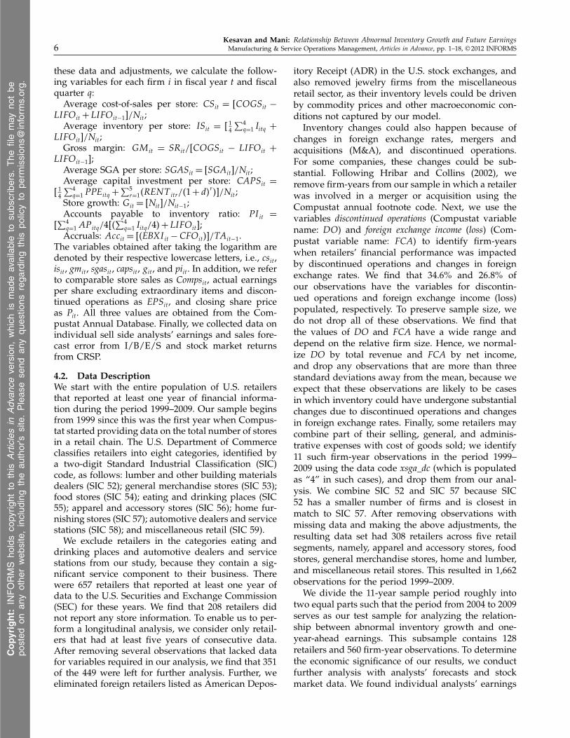
4.2. Data DescriptionWe start with the entire population of U.S. retailersthat reported at least one year of financial informa-tion during the period 1999–2009. Our sample beginsfrom 1999 since this was the first year when Compus-tat started providing data on the total number of storesin a retail chain. The U.S. Department of Commerceclassifies retailers into eight categories, identified bya two-digit Standard Industrial Classification (SIC)code, as follows: lumber and other building materialsdealers (SIC 52); general merchandise stores (SIC 53);food stores (SIC 54); eating and drinking places (SIC55); apparel and accessory stores (SIC 56); home fur-nishing stores (SIC 57); automotive dealers and servicestations (SIC 58); and miscellaneous retail (SIC 59).
We exclude retailers in the categories eating anddrinking places and automotive dealers and servicestations from our study, because they contain a sig-nificant service component to their business. Therewere 657 retailers that reported at least one year ofdata to the U.S. Securities and Exchange Commission(SEC) for these years. We find that 208 retailers didnot report any store information. To enable us to per-form a longitudinal analysis, we consider only retail-ers that had at least five years of consecutive data.After removing several observations that lacked datafor variables required in our analysis, we find that 351of the 449 were left for further analysis. Further, weeliminated foreign retailers listed as American Depos-
itory Receipt (ADR) in the U.S. stock exchanges, andalso removed jewelry firms from the miscellaneousretail sector, as their inventory levels could be drivenby commodity prices and other macroeconomic con-ditions not captured by our model.
Inventory changes could also happen because ofchanges in foreign exchange rates, mergers andacquisitions (M&A), and discontinued operations.For some companies, these changes could be sub-stantial. Following Hribar and Collins (2002), weremove firm-years from our sample in which a retailerwas involved in a merger or acquisition using theCompustat annual footnote code. Next, we use thevariables discontinued operations (Compustat variablename: DO) and foreign exchange income (loss) (Com-pustat variable name: FCA) to identify firm-yearswhen retailers’ financial performance was impactedby discontinued operations and changes in foreignexchange rates. We find that 34.6% and 26.8% ofour observations have the variables for discontin-ued operations and foreign exchange income (loss)populated, respectively. To preserve sample size, wedo not drop all of these observations. We find thatthe values of DO and FCA have a wide range anddepend on the relative firm size. Hence, we normal-ize DO by total revenue and FCA by net income,and drop any observations that are more than threestandard deviations away from the mean, because weexpect that these observations are likely to be casesin which inventory could have undergone substantialchanges due to discontinued operations and changesin foreign exchange rates. Finally, some retailers maycombine part of their selling, general, and adminis-trative expenses with cost of goods sold; we identify11 such firm-year observations in the period 1999–2009 using the data code xsga_dc (which is populatedas “4” in such cases), and drop them from our anal-ysis. We combine SIC 52 and SIC 57 because SIC52 has a smaller number of firms and is closest inmatch to SIC 57. After removing observations withmissing data and making the above adjustments, theresulting data set had 308 retailers across five retailsegments, namely, apparel and accessory stores, foodstores, general merchandise stores, home and lumber,and miscellaneous retail stores. This resulted in 1,662observations for the period 1999–2009.
We divide the 11-year sample period roughly intotwo equal parts such that the period from 2004 to 2009serves as our test sample for analyzing the relation-ship between abnormal inventory growth and one-year-ahead earnings. This subsample contains 128retailers and 560 firm-year observations. To determinethe economic significance of our results, we conductfurther analysis with analysts’ forecasts and stockmarket data. We found individual analysts’ earnings
Copyright:
INFORMS
holdsco
pyrig
htto
this
Articlesin
Adv
ance
version,
which
ismad
eav
ailableto
subs
cribers.
The
filemay
notbe
posted
onan
yothe
rweb
site,includ
ing
the
author’s
site.Pleas
ese
ndan
yqu
estio
nsrega
rding
this
policyto
perm
ission
s@inform
s.org.
Kesavan and Mani: Relationship Between Abnormal Inventory Growth and Future EarningsManufacturing & Service Operations Management, Articles in Advance, pp. 1–18, © 2012 INFORMS 7
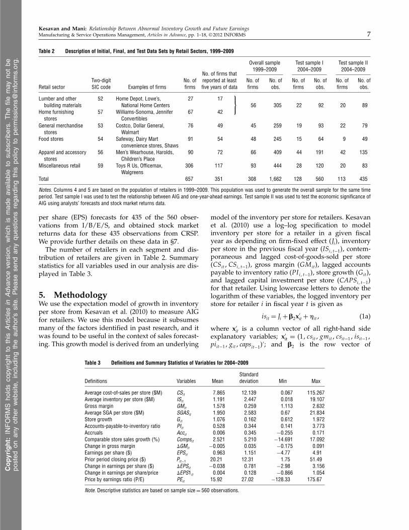
Table 2 Description of Initial, Final, and Test Data Sets by Retail Sectors, 1999–2009
Overall sample Test sample I Test sample II1999–2009 2004–2009 2004–2009
No. of firms thatTwo-digit No. of reported at least No. of No. of No. of No. of No. of No. of
Retail sector SIC code Examples of firms firms five years of data firms obs. firms obs. firms obs.
Lumber and other 52 Home Depot, Lowe’s, 27 17building materials National Home Centers
Home furnishing 57 Williams-Sonoma, Jennifer 67 42stores Convertibles
56 305 22 92 20 89
General merchandise 53 Costco, Dollar General, 76 49 45 259 19 93 22 79stores Walmart
Food stores 54 Safeway, Dairy Mart 91 54 48 245 15 64 9 49convenience stores, Shaws
Apparel and accessory 56 Men’s Wearhouse, Harolds, 90 72 66 409 44 191 42 135stores Children’s Place
Miscellaneous retail 59 Toys R Us, Officemax, 306 117 93 444 28 120 20 83Walgreens
Total 657 351 308 11662 128 560 113 435
Notes. Columns 4 and 5 are based on the population of retailers in 1999–2009. This population was used to generate the overall sample for the same timeperiod. Test sample I was used to test the relationship between AIG and one-year-ahead earnings. Test sample II was used to test the economic significance ofAIG using analysts’ forecasts and stock market returns data.
per share (EPS) forecasts for 435 of the 560 obser-vations from I/B/E/S, and obtained stock marketreturns data for these 435 observations from CRSP.We provide further details on these data in §7.
The number of retailers in each segment and dis-tribution of retailers are given in Table 2. Summarystatistics for all variables used in our analysis are dis-played in Table 3.
5. MethodologyWe use the expectation model of growth in inventoryper store from Kesavan et al. (2010) to measure AIGfor retailers. We use this model because it subsumesmany of the factors identified in past research, and itwas found to be useful in the context of sales forecast-ing. This growth model is derived from an underlying
Table 3 Definitions and Summary Statistics of Variables for 2004–2009
StandardDefinitions Variables Mean deviation Min Max
Average cost-of-sales per store ($M) CSit 70865 120139 00067 1150267Average inventory per store ($M) ISit 10191 20447 00018 190107Gross margin GMit 10578 00259 10113 20632Average SGA per store ($M) SGASit 10950 20583 0067 210834Store growth Git 10076 00162 00612 10972Accounts-payable-to-inventory ratio PIit 00528 00344 00141 30773Accruals Accit 00006 00345 −00255 00171Comparable store sales growth (%) Compsit 20521 50210 −140691 170092Change in gross margin ãGMit −00005 00035 −00175 00091Earnings per share ($) EPSit 00963 10151 −4077 4091Prior period closing price ($) Pit−1 20021 12031 1075 51049Change in earnings per share ($) ãEPSit −00038 00781 −2098 30156Change in earnings per share/price ãEPS1it 00004 00128 −00866 10054Price by earnings ratio (P/E) PEit 15092 27002 −128033 175067
Note. Descriptive statistics are based on sample size = 560 observations.
model of the inventory per store for retailers. Kesavanet al. (2010) use a log–log specification to modelinventory per store for a retailer in a given fiscalyear as depending on firm-fixed effect (Ji5, inventoryper store in the previous fiscal year (ISi1 t−15, contem-poraneous and lagged cost-of-goods-sold per store(CSit1CSi1 t−15, gross margin (GM it5, lagged accountspayable to inventory ratio (PI i1 t−15, store growth (Git5,and lagged capital investment per store (CAPSi1 t−15for that retailer. Using lowercase letters to denote thelogarithm of these variables, the logged inventory perstore for retailer i in fiscal year t is given as
isit = Ji +Â2x′
it +�it1 (1a)
where x′it is a column vector of all right-hand side
explanatory variables; x′it = 411 csit1gmit1 csit−11 isit−11
piit−11git1 capsit−15′; and Â2 is the row vector of
Copyright:
INFORMS
holdsco
pyrig
htto
this
Articlesin
Adv
ance
version,
which
ismad
eav
ailableto
subs
cribers.
The
filemay
notbe
posted
onan
yothe
rweb
site,includ
ing
the
author’s
site.Pleas
ese
ndan
yqu
estio
nsrega
rding
this
policyto
perm
ission
s@inform
s.org.

Kesavan and Mani: Relationship Between Abnormal Inventory Growth and Future Earnings8 Manufacturing & Service Operations Management, Articles in Advance, pp. 1–18, © 2012 INFORMS
the corresponding coefficients, Â2 = 4�201�211�221�231�241�251�261�275
′.This underlying levels model is then first differ-
enced to obtain the following growth model:
ãisit =ãx′
itÂ2 +ã�it0 (1b)
Here ã denotes the change in logged variable in fiscalyear t from fiscal year t − 1.
One may treat all coefficients Â2 in the above regres-sion as being firm specific, i.e., allowing the sensitivityof inventory per store to different factors such as cogsper store, gross margin, capital investment per store,etc., to vary from retailer to retailer. However, to esti-mate such a model, we would need a long time-seriesof observations for each retailer. Because our analy-sis uses annual data, we would need several decadesworth of data for each retailer to estimate such amodel. To overcome the paucity of data, we assumethat all firms in a given segment are homogeneous,i.e., we assume that the coefficients Â2 are identical forall retailers within a given segment and estimate thesecoefficients at the segment level. Thus, our estimationequation is
ãisit =ãx′
itÂ21 s4i5 +ã�it1 (1c)
where s4i5 denotes the corresponding segment-specific coefficients for firm i.
We can now obtain the expected logged inventorygrowth from the above equation, E4ãisit5, and thencompute abnormal inventory growth in the followingway. Let 8ISit/ISit−1 − 19 denote the actual inven-tory per store growth and AIGit = 48ISit/ISit−1 − 19 −
8exp4E4ãisit55 − 195 denote the abnormal inventoryper store growth or, in short, abnormal inventorygrowth for a retailer i in fiscal year t. We estimateEquation (1c) and use the coefficients to computeabnormal inventory growth. Thus, AIGit > 0 impliesthat retailer i has abnormally high inventory growthwhereas AIGit < 0 implies that retailer i has abnor-mally low inventory growth compared to the norm ofthe segment to which the retailer belongs, after con-trolling for firm-level differences.
Kesavan et al. (2010) showed that historical grossmargin contains information valuable to forecastsales. Further, they showed that inventory and grossmargin are highly correlated for retailers, so we cal-culate abnormal change in gross margin in a similarmanner as AIG and use it as a control variable in ouranalysis. Similar to Equation (1c), the first differencedequation for gross margin can be written as
ãgmit =ãx′
itÂ31 s4i5 +ã�it1 (2)
where ãx′it = 411ãcsit1ãisit1ãgmit−15
′. We calculate ab-normal change in gross margin (ACGM) for retailer i
in fiscal year t as ACGMit = 48GMit/GMit−1 − 19 −
8exp4E4ãgmit55− 195.Next, we explain the data used to measure AIGit−1
from (1c). We use data till fiscal year t − 2 to esti-mate (1c). We avoid data from fiscal year t − 1 inthe estimation because firms announce their financialresults at different times of the year, which could leadto a potential look-ahead that could bias our resultsabout the relationship between AIG and one-year-ahead earnings. Once a retailer’s financial results areannounced for fiscal year t − 1, we use our coeffi-cient estimates to measure the AIGit−1 for that retailer.We follow this process for all retailers in our test sam-ple, i.e., t = 2004, 2009. We follow a similar approachto obtain ACGM it−1.
We considered two different techniques to estimateEquations (1c) and (2). We used the instrument vari-able generalized least squares (IVGLS) method usedin Kesavan et al. (2010) to estimate the equations andalso a simpler single-equation technique, a general-ized least squares (GLS) method, as a cross-check. Wefound the results to be similar. Because the IVGLSmethod requires defining an additional equation con-taining new variables, we choose to report the resultsof the GLS technique that is simpler to implement andexplain. The GLS method handles heteroskedasticityand panel-specific autocorrelation in the data.
Table 4 reports sample results of our estimationof Equations (1c) and (2) using data from 2002–2007.These coefficient estimates were then used to calcu-late AIG and ACGM for fiscal year 2008, which arethen used to predict earnings for fiscal year 2009.Figure 1(a) presents the histogram of AIG for allretailers in our EPS sample (n = 560) during theperiod t = 20041 0 0 0 12009. We find that 63% of retail-ers have AIG > 0 and 37% have AIG < 0. We findthat the average, lowest, highest, and standard devia-tions of AIG for this time period are 2.28%, −17033%,26.21%, and 8.76%, respectively. Descriptive statisticsare reported in Table 5. For the average retailer in oursample, with $1.2 million of inventory per store, themean (2.28%) and mean plus one standard deviation(11.04%) of AIG correspond to $27,380 and $132,480 ofabnormal inventory per store. The average AIG acrossthe different retail segments for the same period is2.67% (apparel), 0.17% (food), 2.32% (general), 2.69%(home), and 1.63% (miscellaneous). The magnitudesof correlations between AIG and sales per store, salesgrowth, and store growth are less than 0.21. Theseweak correlations indicate that AIG is not specific toretailer characteristics such as average sales volumeper store or growth rate. We also find that the rel-ative rank of retailers based on AIG varies consid-erably from year to year, indicating that AIG is notpersistent.
Copyright:
INFORMS
holdsco
pyrig
htto
this
Articlesin
Adv
ance
version,
which
ismad
eav
ailableto
subs
cribers.
The
filemay
notbe
posted
onan
yothe
rweb
site,includ
ing
the
author’s
site.Pleas
ese
ndan
yqu
estio
nsrega
rding
this
policyto
perm
ission
s@inform
s.org.

Kesavan and Mani: Relationship Between Abnormal Inventory Growth and Future EarningsManufacturing & Service Operations Management, Articles in Advance, pp. 1–18, © 2012 INFORMS 9
Table 4 Estimation Results of Inventory and Gross Margin Equation for Each Retail Segment, 2002–2007
Retail industry segment
Apparel and accessory General merchandise Home furnishing MiscellaneousEquation Variables stores Food stores stores stores retail
Inventory equation Intercept −00009∗∗ −00010∗∗ −00011∗∗∗ −00008∗∗∗ −00002∗∗
4000035 4000045 4000015 4000015 4000015ãisit−1 −00049∗∗∗ −00044 −00017∗ −00021∗∗∗ −00169∗∗∗
4000115 4000845 4000095 4000025 4000295ãcsit 00880∗∗∗ 00771∗∗∗ 10067∗∗∗ 00902∗∗∗ 00594∗∗∗
4000365 4000635 4000295 4000435 4000175ãgmit 00115∗ 00149∗∗∗ −00602∗∗∗ −00158∗ 00312∗∗
4000615 4000255 4001315 4000945 4001415ãcsit−1 00094∗∗ 00252∗∗∗ 00046∗ 00042 00289∗∗∗
4000395 4000675 4000255 4000845 4000385ãpiit−1 −00014 −00071∗ −00056∗∗ −00055∗ −00031∗∗
4000225 4000395 4000235 4000315 4000125ãgit −00099∗∗ −00194∗∗ −00070∗∗ −00075∗ −00276∗∗∗
4000375 4000645 4000285 4000405 4000365ãcapsit−1 00056 00117∗∗ 00065∗∗ 00024 00057∗∗∗
4000395 4000385 4000325 4000625 4000135Gross margin equation Intercept 00006∗∗∗ 00003∗∗ 2e-4∗∗∗ 00002∗∗∗ 00012∗∗∗
4000015 4000015 (3e-5) (4e-4) 4000015ãgmit−1 00038∗∗ 00134∗∗ 00210∗∗∗ 00189∗∗ −00012
4000195 4000415 4000165 4000635 4000225ãcsit 00187∗∗∗ 00123∗∗∗ 00039∗∗∗ 00012∗ −00684∗∗∗
4000225 4000115 4000095 4000075 4000165ãisit −00158∗∗∗ −00148∗∗∗ −00035∗∗ −00012∗∗ −00541∗∗∗
4000175 4000075 4000155 4000065 4000165
n 215 110 112 107 211
Notes. We refer to Equations (1c) and (2) as the inventory equation and gross margin equation. These equations are estimated on a rolling horizon basis witha five-year constant window. The estimation results above were generated based on data from 2002–2007. These coefficients are used to generate abnormalinventory growth for year 2008, which is in turn used to predict earnings, analysts’ bias, and stock market returns for 2009. All regressions are run aftercontrolling for panel specific autocorrelation.
∗∗∗p < 00001; ∗∗p < 0005; ∗p < 001.
5.1. Abnormal Days of InventoryWe use the abnormal days of inventory (AbI) mea-sure proposed by Chen et al. (2007) as an alternatemeasure of abnormal inventory growth. Chen et al.(2007) defined abnormal days of inventory (AbIit )as the normalized deviation of the days of inventory(DOIit5 of retailer i in fiscal year t from the averagedays of inventory of its industry peers:
AbIit =4DOIit −DOI st5
DOI st
0
Here DOIst and DOIst are the average and stan-dard deviations of days of inventory of all retail-ers in the segment s to which retailer i belongs.If AbIit > 0 (AbIit < 05, then retailer i holds inventorylonger (shorter) than the segment norm in year t. Theaverage, lowest, highest, and standard deviations ofAbI during 2004–2009 are 0.23, −2063, 2.09, and 1.23,respectively. The average abnormal days of inventoryacross the different segments for the same period is
0.15 (apparel), 0.07 (food), 0.15 (general), 0.17 (home),and 0.11 (miscellaneous).
The main difference between the AIG and AbI met-rics is that the former controls for factors such asgross margin, capital investment, store growth, andaccounts payable that have been identified as impor-tant factors driving inventory levels in operations lit-erature, whereas the AbI metric does not. However,the use of lagged variables in the regression used toestimate AIG requires at least three years of data tomeasure AIG for a retailer. The AbI metric, however,can be computed even for a retailer that has just oneyear of data. We use both metrics to test the relation-ship between abnormal inventory growth and one-year-ahead earnings.
6. ResultsIn this section, we discuss results of our statisticaltests of the relationship between AIG and one-year-ahead earnings. Several researchers in accountinghave used a first-order autoregressive model for
Copyright:
INFORMS
holdsco
pyrig
htto
this
Articlesin
Adv
ance
version,
which
ismad
eav
ailableto
subs
cribers.
The
filemay
notbe
posted
onan
yothe
rweb
site,includ
ing
the
author’s
site.Pleas
ese
ndan
yqu
estio
nsrega
rding
this
policyto
perm
ission
s@inform
s.org.
Kesavan and Mani: Relationship Between Abnormal Inventory Growth and Future Earnings10 Manufacturing & Service Operations Management, Articles in Advance, pp. 1–18, © 2012 INFORMS
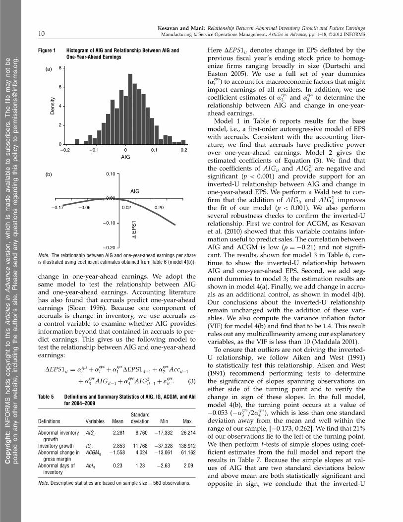
Figure 1 Histogram of AIG and Relationship Between AIG andOne-Year-Ahead Earnings
–0.20
–0.10
0.00
0.10
–0.2 –0.10
2
4
6
Den
sity
8
0 0.1
AIG
(a)
(b)
0.2
–0.17 –0.06 0.200.02
AIG
∆ E
PS
1
Note. The relationship between AIG and one-year-ahead earnings per shareis illustrated using coefficient estimates obtained from Table 6 (model 4(b)).
change in one-year-ahead earnings. We adopt thesame model to test the relationship between AIGand one-year-ahead earnings. Accounting literaturehas also found that accruals predict one-year-aheadearnings (Sloan 1996). Because one component ofaccruals is change in inventory, we use accruals asa control variable to examine whether AIG providesinformation beyond that contained in accruals to pre-dict earnings. This gives us the following model totest the relationship between AIG and one-year-aheadearnings:
ãEPS1it = �epso +�
epst +�
eps1 ãEPS1it−1 +�
eps2 Accit−1
+�eps3 AIGit−1 +�
eps4 AIG2
it−1 + �epsit 0 (3)
Table 5 Definitions and Summary Statistics of AIG, IG, ACGM, and AbIfor 2004–2009
StandardDefinitions Variables Mean deviation Min Max
Abnormal inventory AIGit 20281 80760 −170332 260214growth
Inventory growth IGit 20853 110768 −370328 1360912Abnormal change in ACGMit −10558 40024 −130061 610162
gross marginAbnormal days of AbIit 0023 1023 −2063 2009
inventory
Note. Descriptive statistics are based on sample size = 560 observations.
Here ãEPS1it denotes change in EPS deflated by theprevious fiscal year’s ending stock price to homog-enize firms ranging broadly in size (Durtschi andEaston 2005). We use a full set of year dummies(�eps
t 5 to account for macroeconomic factors that mightimpact earnings of all retailers. In addition, we usecoefficient estimates of �eps
3 and �eps4 to determine the
relationship between AIG and change in one-year-ahead earnings.
Model 1 in Table 6 reports results for the basemodel, i.e., a first-order autoregressive model of EPSwith accruals. Consistent with the accounting liter-ature, we find that accruals have predictive powerover one-year-ahead earnings. Model 2 gives theestimated coefficients of Equation (3). We find thatthe coefficients of AIGit and AIG2
it are negative andsignificant (p < 00001) and provide support for aninverted-U relationship between AIG and change inone-year-ahead EPS. We perform a Wald test to con-firm that the addition of AIGit and AIG2
it improvesthe fit of our model (p < 00001). We also performseveral robustness checks to confirm the inverted-Urelationship. First we control for ACGM, as Kesavanet al. (2010) showed that this variable contains infor-mation useful to predict sales. The correlation betweenAIG and ACGM is low (� = −0021) and not signifi-cant. The results, shown for model 3 in Table 6, con-tinue to show the inverted-U relationship betweenAIG and one-year-ahead EPS. Second, we add seg-ment dummies to model 3; the estimation results areshown in model 4(a). Finally, we add change in accru-als as an additional control, as shown in model 4(b).Our conclusions about the inverted-U relationshipremain unchanged with the addition of these vari-ables. We also compute the variance inflation factor(VIF) for model 4(b) and find that to be 1.4. This resultrules out any multicollinearity among our explanatoryvariables, as the VIF is less than 10 (Maddala 2001).
To ensure that outliers are not driving the inverted-U relationship, we follow Aiken and West (1991)to statistically test this relationship. Aiken and West(1991) recommend performing tests to determinethe significance of slopes spanning observations oneither side of the turning point and to verify thechange in sign of these slopes. In the full model,model 4(b), the turning point occurs at a value of−00053 4−�
eps3 /2�eps
4 5, which is less than one standarddeviation away from the mean and well within therange of our sample, [−00173100262]. We find that 21%of our observations lie to the left of the turning point.We then perform t-tests of simple slopes using coef-ficient estimates from the full model and report theresults in Table 7. Because the simple slopes at val-ues of AIG that are two standard deviations belowand above mean are both statistically significant andopposite in sign, we conclude that the inverted-U
Copyright:
INFORMS
holdsco
pyrig
htto
this
Articlesin
Adv
ance
version,
which
ismad
eav
ailableto
subs
cribers.
The
filemay
notbe
posted
onan
yothe
rweb
site,includ
ing
the
author’s
site.Pleas
ese
ndan
yqu
estio
nsrega
rding
this
policyto
perm
ission
s@inform
s.org.

Kesavan and Mani: Relationship Between Abnormal Inventory Growth and Future EarningsManufacturing & Service Operations Management, Articles in Advance, pp. 1–18, © 2012 INFORMS 11
Table 6 Relationship Between AIG and One-Year-Ahead Earnings, 2004–2009
Dependent variable: Change in EPS1Independentvariables Model 1 Model 2 Model 3 Model 4(a) Model 4(b)
Intercept 00093∗∗∗ 00007∗∗∗ 00008∗∗∗ 00010∗∗∗ 00009∗∗∗
4000095 4000015 4000015 4000025 4000025ãEPS1it−1 00074∗∗∗ 00067∗∗∗ 00075∗∗∗ 00055∗∗ 00046∗∗
4000155 4000145 4000155 4000185 4000185AIGit−1 −00076∗∗∗ −00075∗∗∗ −00097∗∗∗ −00103∗∗∗
4000085 4000135 4000115 4000125AIG2
it−1 −10042∗∗∗ −10127∗∗∗ −00991∗∗∗ −00980∗∗∗
4000985 4000975 4001055 4001095ACGMit−1 00111∗∗∗ 00049∗∗ 00063∗∗
4000235 4000245 4000255Accit−1 −10501∗∗∗ −10722∗∗∗ −10581∗∗∗ −10534∗∗∗ −10774∗∗∗
4000755 4001245 4001435 4001265 4001335ãAccit−1 −00300∗∗∗
4000885
Segment dummies No No No Yes YesWald �2 3,531.80 8,179.53 9,789.20 11,920.09 24,830.96n 560 560 560 560 560
Notes. All regressions are run after controlling for year fixed effects and panel specific auto-correlation. Model 4(b) is the full model with all the controls. Standard errors are reported inparentheses below the coefficients.
∗∗∗p < 00001; ∗∗p < 0005; ∗p < 001.
relationship between AIG and one-year-ahead earn-ings is supported within the range of our data, andnot driven by outliers.
We use the coefficient estimates (�eps3 1�
eps34 5 from the
full model to graphically illustrate the inverted-U rela-tionship between AIG and the change in one-year-ahead earnings as shown in Figure 1(b). The mean AIGin our sample is 0.023 and the standard deviation is0.09. At the mean, the impact of increasing AIG by0.01 leads to a decrease in the dependent variable, i.e.,the change in EPS scaled by price, by 0.0016. To putthis number in perspective, we multiply it by the sam-ple average price-to-earnings ratio of 16 to obtain thepercentage decrease in EPS in the following year com-pared to the average retailer. This shows that a retailerwhose AIG was 0.01 more than the average AIG in our
Table 7 t-Tests for Simple Slopes at Different Values of AIG
AIG valuea Simple slope Standard error Significance
−00173 00236 00071 30324∗∗
−00152 00196 00072 20730∗∗
−00065 00024 00019 10247−00053b 00000 00017 00000
0.023 −00148 00018 −80215∗∗∗
0.111 −00320 00031 −100313∗∗∗
0.198 −00492 00041 −110989∗∗∗
0.262 −00617 00051 −120085∗∗∗
aThe AIG values are chosen to span the observations on each side of theturning point The simple slope and turning point are calculated based onmodel 4(b).
bTurning point.∗∗∗p < 00001; ∗∗p < 0005; ∗p < 001.
sample would find its earnings per share to be 2.56%lower than the retailer with the average AIG, holdingeverything else constant. At a higher level of distri-bution, corresponding to the mean plus two times thestandard deviation, increasing AIG by 0.01 is associ-ated with a decrease in EPS of 8.2% in the followingyear. At a lower distribution level (corresponding tothe mean minus two times the standard deviation),further decreasing AIG by 0.01 unit is associated witha 3.4% decline in EPS in the next year.
On two attributes of the inverted-U relationshipwe further elaborate. First, the turning point occur-ring at a value less than zero is interesting. Recallthat our results are picking up the dominant effectas we cannot control for unobservable factors suchas management’s private information about futuredemand, service level, or lost sales. Thus, we con-jecture that the region [−0005310] is dominated byretailers who became leaner. That is, these retailerswere able to reduce their inventory levels withoutsubstantial reduction in service level. To ensure thatthis result is not an artifact of the AIG metric, were-test model 4(b) by substituting the AbI metric forthe AIG metric, based on Chen et al. (2007), andfind qualitatively similar results. The coefficients ofAbIit and AbI 2
it are −00005 and −00004 (p < 00001),respectively, indicating the existence of an inverted-Ushaped relationship between AbI and change in one-year-ahead earnings. Similar to results obtained withthe AIG metric, we find the turning point to be neg-ative and within one standard deviation of the mean.
Copyright:
INFORMS
holdsco
pyrig
htto
this
Articlesin
Adv
ance
version,
which
ismad
eav
ailableto
subs
cribers.
The
filemay
notbe
posted
onan
yothe
rweb
site,includ
ing
the
author’s
site.Pleas
ese
ndan
yqu
estio
nsrega
rding
this
policyto
perm
ission
s@inform
s.org.

Kesavan and Mani: Relationship Between Abnormal Inventory Growth and Future Earnings12 Manufacturing & Service Operations Management, Articles in Advance, pp. 1–18, © 2012 INFORMS
The values of the turning point, minimum, and maxi-mum values of AbI are −0063, −2063, and 2.09, respec-tively. The results with AbI metric are reported in thispaper’s online supplement (available at http://dx.doi.org/10.1287/msom.1120.0389). Thus, our resultsappear to be robust to the method used to computeabnormal inventory carried by retailers.
Second, consistent with Chen et al. (2007), whoexamined long-term stock market returns of retail-ers, we find that our strongest results are for retailerswith abnormally high inventory growth, whose sub-sequent performance was poor. Some retailers in thisregion (AIG > 0) likely were able to increase their ser-vice level to more closely approximate the optimallevel, and subsequently increased their profitability.However, those retailers appear to be dominated byretailers who simply had excess inventory.
Because AIG predicts sales (Kesavan et al. 2010),and earnings are a function of sales, we want to deter-mine if the relationship between AIG and earningsare driven only by AIG’s ability to predict sales, orif AIG might predict earnings for additional reasons.As we argue in §3, AIG might also provide reasonsto predict higher expenses such as for advertising toclear merchandise, or for holding costs and inven-tory write-downs. Because these expenses are notreadily available as separate line items in retail-ers’ income statements, we test this argument indi-rectly by adding one-year-ahead sales growth (SGit5to model 4(b) to control for changes in EPS due to anychange in sales for a given retailer, as follows:
ãEPS1it = �epso +�
epst +�
eps1 ãEPS1it−1 +�
eps2 Accit−1
+�eps3 AIGit−1 +�
eps4 AIG2
it−1 +�eps5 ACGMi1 t−1
+�eps6 ãAccit−1 +�
eps7 SGit + �
epsit 0 (4)
Our use of one-year-ahead sales growth makes thisanalysis conservative because it tests whether AIGcan predict expenses that are not correlated with rev-enues. Model 5 in Table 8 reports the results of thisregression. We find that both the linear and quadraticterms of AIG are significant (p < 00001). We replacesales growth in period t with comparable store salesduring that period and obtain similar results, shownin model 6 of Table 8. Thus, we conclude that AIGpredicts earnings for retailers because it has infor-mation useful to predict sales as well as expenses ofretailers.
Additional robustness checks to show that theexplanatory power of abnormal inventory measureexists even when standard accounting “abnormalaccruals” measures (Jones and Modified Jones mod-els) are used as control variables is provided in theonline supplement.
Table 8 Relationship Between AIG and Future Expenses, 2004–2009
Change in EPS1
Independent variables Model 5 Model 6
Intercept 00079∗∗∗ 00011∗∗∗
4000085 4000025ãEPS1it−1 00048∗∗ 00034∗
4000155 4000195AIGit−1 −00101∗∗∗ −0092∗∗∗
4000085 4000185
AIG2it−1 −00822∗∗∗ 10249∗∗∗
4000715 4001555ACGMit−1 00067∗∗ 00091∗∗
4000245 4000385ãAccit−1 −00353∗∗∗ −00901∗∗∗
4000595 4001325Accit−1 −10178∗∗∗ −20474∗∗∗
4001535 4001975SGit 00091∗∗∗
4000075COMPSit 00019∗∗∗
4000015
Segment dummies Yes YesWald �2 24,853.60 20,621.27n 560 494
Notes. Models 5 and 6 add sales growth (SGit 5 and comparable storesales growth (COMPSit 5 to model 4(b) shown in Table 6, respectively.Because SGit and COMPSit are contemporaneous to the dependent variable,ãEPS1it , models 5 and 6 test if abnormal inventory growth can predict theportion of expense changes not correlated with revenue growth.
∗∗∗p < 00001; ∗∗p < 0005; ∗p < 001.
7. Economic Significance ofInformation Contained in AIG
In this section, we investigate the economic signif-icance of our finding. First, we examine whetherequity analysts take information contained in AIGinto account when generating earnings forecasts. Sec-ond, we test whether stock prices incorporate thisinformation. The former test would show whethereven sophisticated investors could benefit from know-ing information contained in AIG, and the latterwould indicate whether AIG can form the basis foran investment strategy.
7.1. Do Equity Analysts Ignore Information inAbnormal Inventory Growth in EPSForecasts?
We examine whether or not equity analysts ignoreinformation contained in AIG as follows. Analystsissue earnings forecasts at different times during ayear and revise those forecasts as more informationbecomes available. These forecasts are time stampedwith the dates they are issued. Because financial infor-mation for the previous fiscal year are released on theearnings announcement date (EAD), the informationrequired to compute AIG for a retailer is available
Copyright:
INFORMS
holdsco
pyrig
htto
this
Articlesin
Adv
ance
version,
which
ismad
eav
ailableto
subs
cribers.
The
filemay
notbe
posted
onan
yothe
rweb
site,includ
ing
the
author’s
site.Pleas
ese
ndan
yqu
estio
nsrega
rding
this
policyto
perm
ission
s@inform
s.org.

Kesavan and Mani: Relationship Between Abnormal Inventory Growth and Future EarningsManufacturing & Service Operations Management, Articles in Advance, pp. 1–18, © 2012 INFORMS 13
after its EAD. If analysts incorporate into their fore-casts information from lagged AIG, then their fore-casts issued subsequent to EAD should not generateerrors that can be predicted by lagged AIG. If, how-ever, they do not incorporate this information, thenlagged AIG will have predictive power over theirforecast errors.
Our tests are conducted using the I/B/E/S detailed(individual) forecasts of annual EPS. We performthis analysis using data obtained for fiscal years2004–2009. We consider analysts’ earnings forecastsfor the forthcoming fiscal year issued after a retailer’sEAD in the prior fiscal year. In some cases, analystsmight have to wait till retailers file their 10-K state-ment with the SEC to have access to their finan-cial statements. To be conservative, we drop anyanalyst forecasts made before the SEC filing date,as well. We obtain the SEC filing date for eachretailer from Morningstar Document Research, acces-sible from http://www.10kwizard.com/. If multipleforecasts are made by an analyst for a retailer, we usethe most recent forecast, as that should contain thelatest information available to the analyst.
We find that analysts’ forecasts were available for435 observations of our 560 total. For each firm-year,we determine the median of analysts’ forecasts madefor each of the m= 1 to 12 months after EAD for fiscalyear t− 1, and use that as a single consensus forecastfrom which to generate analysts’ consensus forecasterror. We compute forecast errors by subtracting theconsensus EPS forecast from realized EPS. We alsodeflate the forecast error by the previous fiscal year’sending stock price (Gu and Wu 2003). For forecastsmade three months after the EAD for fiscal year t−1,the average, standard deviation, minimum, and max-imum deflated analysts’ forecast error between 2004and 2009 are −00038, 0.163, −00911, and 0.052, respec-tively. The average forecast error of −00038 shows thatanalysts are optimistic, on average, consistent withprior accounting literature.
Next, we statistically test whether analysts’ forecasterrors are biased, as predicted by lagging AIG, byrunning the following regression:
F Eitm = �0 +�t +�1AIGi1 t−1 +�2AIG2i1 t−1
+�3ACGMi1 t−1 +�4Acci1 t−1 +ÃY′
itm +�it0 (5)
Here F Eitm is the deflated forecast error of analysts’consensus forecast generated m months before theend of fiscal year t for retailer i. The �0 term capturesthe bias common to all retailers, �t is the bias specificto a given fiscal year, �1 and �2 capture that bias cor-related with the previous year’s AIG, �3 is the biascorrelated with the previous year’s ACGM, and Y′
itm
is the vector of control variables found to be related toforecast bias in the accounting literature (Gu and Wu
Table 9 Bias in Deflated Analysts’ EPS Forecasts Due to Lagged AIG,2004–2009
Dependent variable: deflated analyst forecasterror m months after EADt−1Independent
variables m = 1 month m = 3 months m = 6 months
Intercept −00057∗∗∗ −00031∗∗∗ −00027∗∗∗ −00035∗∗∗
4000115 4000065 4000045 4000065AIGit−1 −00098∗∗∗ −00074∗∗∗ −00043∗∗ −00031∗
4000095 4000085 4000185 4000175AIG2
it−1 −00067 −00071 −00070 −000814000915 4000875 4000715 4001015
ACGMit−1 00191∗∗∗ 00183∗∗∗ 00271∗∗ 00161∗
4000515 4000415 4001215 4000905Accit−1 00075∗∗∗ −00066∗∗∗ −00026∗∗ −00018∗
4000115 4000135 4000125 4000015DISPitm 10102∗∗∗ −00854∗∗∗ −00378∗∗ −00218∗∗
4001485 4001595 4001675 4001035LGMVit−1 00112∗∗∗ 00012∗∗∗ 00005∗∗∗ 00003∗∗
4000145 4000025 4000015 4000015LGFFWit−1 −00049 −00010 −00005 −00004
4000445 4000185 4000105 4000115Lossit−1 −00075∗∗ −00035∗∗ −00023∗∗ −00017∗
4000325 4000165 4000115 4000095SUE_1it−1 00481∗∗ 00141∗ 00031∗ 00028∗
4002115 4000715 4000185 4000155SUE_2it−1 00314 −00027 00003 00005
4002995 4000245 4000105 4000155FE_SALEitm 91e-4∗
(5.2e-4)
n 391 435 435 375Wald (�2) 8,479.63 5,345.24 2,141.14 2,402.65
Notes. FE_SALEitm = deflated analyst sales forecast error. This regres-sion also includes the following control variables from Gu and Wu (2003):DISPitm = analyst dispersion, i.e., the standard deviation of deflatedforecasts for each month m in year t ; LGMV it−1 = log(market value);LGFFW it−1 = log(analyst coverage); Lossit−1 = an ex ante loss dummy vari-able that takes a value of 1 if the forecasted current earnings are negative and0 otherwise; SUE_1it−1 and SUE_2it−1 are price deflated lag-one and lag-twounexpected earnings from a seasonal random walk model. All regressionsare run after controlling for year fixed effects and panel-specific autocorrela-tion. Standard errors are reported in parentheses below the coefficients.
∗∗∗p < 00001; ∗∗p < 0005; ∗p < 001.
2003). These variables include dispersion among ana-lysts’ forecasts, analyst coverage, market value, unex-pected earnings from a seasonal random-walk model,and a dummy variable to capture ex ante any expec-tation of loss in earnings. Detailed descriptions of thevariables are provided in the note below Table 9.
We estimate (5) by using the GLS technique. Table 9provides the formal statistical test of the relationbetween analysts’ forecast errors and lagged AIG. Wefind that the bias in analysts’ forecasts due to AIGcontinues to remain significant (p < 0005) up to sixmonths from the prior fiscal year’s EAD, as shown inTable 9. The magnitude of reported coefficients maybe interpreted in the following way. Consider the fore-casts made m= 6 months after EAD for the prior fiscal
Copyright:
INFORMS
holdsco
pyrig
htto
this
Articlesin
Adv
ance
version,
which
ismad
eav
ailableto
subs
cribers.
The
filemay
notbe
posted
onan
yothe
rweb
site,includ
ing
the
author’s
site.Pleas
ese
ndan
yqu
estio
nsrega
rding
this
policyto
perm
ission
s@inform
s.org.

Kesavan and Mani: Relationship Between Abnormal Inventory Growth and Future Earnings14 Manufacturing & Service Operations Management, Articles in Advance, pp. 1–18, © 2012 INFORMS
year (m= 6, column 3 in Table 9). We find the coeffi-cient of AIG to be −00043 (p < 0005). This implies that,for an average retailer in our sample with a price-to-earnings ratio of 16, a one-standard-deviation increasein AIG is associated with an increase in forecast errorsequivalent to 6.19% of earnings. We do not find thequadratic term of AIG to be significant, indicating alinear relationship between AIG and analysts’ forecasterrors. Finally, we find that coefficients of four of thesix control variables are significant and in the samedirections as reported in prior accounting literature(Gu and Wu 2003). The remaining two control vari-ables are directionally similar but not significant. Ourresult that analysts miss information in inventory use-ful to predict earnings is consistent with the resultsdocumented in accounting literature (Bradshaw et al.2001, Abarbanell and Bushee 1997).
Next, we want to determine whether our resultthat AIG predicts bias in analysts’ EPS forecasts isdriven by analysts’ failure to incorporate only infor-mation contained in AIG to predict sales, as shown byKesavan et al. (2010), or to predict expenses as well.To do so, we pick analysts’ sales forecasts made m= 6months after the EAD for the prior fiscal year (col-umn 4, Table 9). Sales forecasts were available foronly 375 of the 435 total observations in our sample.We add contemporaneous error in analysts’ sales fore-casts to Equation (5) for this sample (m= 6) and findthat AIG remains a significant predictor of bias in ana-lysts’ forecasts of EPS (p < 001) indicating that analystsalso fail to fully incorporate information in inven-tory that is useful to predict expenses for retailers.We obtain consistent results for m = 1 and 3 months,as well, with stronger results (p < 0005).
To summarize, our results show that analysts fail tofully incorporate information in AIG to predict earn-ings. These results not only support the results fromKesavan et al. (2010), but add to them by showingthat analysts fail to fully utilize information containedin AIG to predict expenses, as well.
7.2. Does an Investment Strategy Based onAIG Yield Abnormal Returns?
In this section, we examine whether investmentsbased on AIG can yield abnormal returns. In otherwords, we examine whether AIG is an “anomaly”variable. The accounting and finance literature defineanomaly variables as those that help to identify pat-terns in stock returns that are not explained by thecapital asset pricing model (CAPM) of Sharpe (1964)and Lintner (1965). Fama and French (2008) sur-veyed various methodologies used to identify anoma-lies in prior literature, and identified two commonapproaches based on the extensive literature. The firstapproach is based on sorting, and the second is basedon regressions. We follow both approaches to examine
whether an investment strategy based on AIG wouldyield abnormal stock returns.
First, consider the approach based on sorting, a sim-ple method that examines how the average abnor-mal monthly returns of stocks vary across the rangeof an anomaly variable (AIG in our case). Thisapproach involves constructing quintile portfolios offirms based on ranks of their AIG in the previous fis-cal year. An important consideration is that all infor-mation required to construct a portfolio for a givenfiscal year is available at the time the portfolio is cre-ated. Because firms file their 10-K statements with theSEC at different times in the year, the informationrequired to construct a portfolio comprising all theretailers in our sample becomes available at differenttimes. For our test sample, we find that the monthof April had the most SEC filings (243), followed byMarch (82) and May (50). The remaining months hadfewer than 20 filings each.
We follow Fama and French (2008) to calculate theabnormal monthly return of each stock in the follow-ing way. First, we match each stock to its benchmarkportfolio using that stock’s size and book-to-marketvalue (BM). The matching benchmark portfolio is oneof 25 portfolios value weighted (VW) by size and BM,obtained from Ken French’s website.1 These 25 bench-mark portfolios are themselves formed at the end ofJune each year, based on the market equity and book-to-market values of all NYSE, AMEX, and NASDAQstocks. The abnormal monthly return of each stock isobtained by subtracting the VW monthly return of thebenchmark portfolio from that of the stock return.
Next, we sort firms in our test sample into port-folios and calculate the average abnormal monthlyreturn of each portfolio, as illustrated here for 2004:We calculate the AIG value for each retailer that fileda 10-K statement with the SEC during the periodMarch–May 2004. Then we sort the retailers into fiveportfolios, P0, P1, …, P4, such that portfolio P0 con-tains firms with AIG in the bottom quintile and port-folio P4 contains firms with AIG in the top quintile.We then compute the equal weighted (EW) averageabnormal monthly return of each portfolio for eachmonth from July 2004 to June 2005. At the end ofJune 2005, we re-sort the firms into the five port-folios based on AIG computed, using 10-K infor-mation released during March–May 2005. We repeatthe process of calculating average abnormal monthlyreturn and re-sorting for each of the years 2005–2009.Thus, we sort firms into portfolios six times during2004–2009, giving us 72 observations of the average
1 Available at http://mba.tuck.dartmouth.edu/pages/faculty/ken.french/data_library.html.
Copyright:
INFORMS
holdsco
pyrig
htto
this
Articlesin
Adv
ance
version,
which
ismad
eav
ailableto
subs
cribers.
The
filemay
notbe
posted
onan
yothe
rweb
site,includ
ing
the
author’s
site.Pleas
ese
ndan
yqu
estio
nsrega
rding
this
policyto
perm
ission
s@inform
s.org.

Kesavan and Mani: Relationship Between Abnormal Inventory Growth and Future EarningsManufacturing & Service Operations Management, Articles in Advance, pp. 1–18, © 2012 INFORMS 15
Table 10 Average Abnormal Returns and t-Statistics for Portfolios Formed Using Sorts on AIG, ACC, and INVG, 2004–2009
Average monthly abnormal returns (AR) t-statistic for AR
High–Low High–LowSorting on P0 P1 P2 P3 P4 (P4–P0) P0 P1 P2 P3 P4 (P4–P0)
AIG 0022 0014 0005 −0045∗ −0070∗∗∗ −0092∗∗∗ 0064 0041 0010 −1075 −3014 −3018ACC 0018 0008 0006 −0020 −0061∗∗ −0079∗∗ 0032 0020 0009 −1056 −2002 −2022INVG 0016 0024 −0010 −0042 −0055∗ −0071∗ 0062 0061 −0019 −0083 −1073 −1075
Notes. We sort stocks into portfolios at the end of June of each year t , and compute value weighted abnormal returns for July of t to June of t + 1. Eachyear, we sort the firms based on each of the anomaly variables into five quintiles (P0 (lowest) to P5 (highest)). We assign firms to matching BM and sizeportfolios using the quintile breakpoints form from Ken French’s website. The abnormal monthly return on a stock is measured net of the value-weight returnon a matching portfolio formed on size and BM. The average monthly equal-weight return for each portfolio is shown above. All returns presented in the tableare expressed as percentages.
∗∗∗p < 00001; ∗∗p < 0005; ∗p < 001.
abnormal monthly return for each portfolio. The aver-age abnormal returns of a portfolio represent the por-tion of anomalous average returns not explained bythe size or BM value of the retailers concerned.
Again we follow Fama and French (2008) to reportthe average of the 72 monthly observations and thet-statistics for each portfolio. The results can be foundin Table 10. We find that the average abnormal returnfor portfolios P0 to P4, based on AIG, vary between0.22% and −0070%. We note that the average abnor-mal returns of portfolios P3 and P4 are significant atp < 001 and p < 0001, respectively, whereas the aver-age abnormal returns for the rest of the portfoliosare not statistically significant. This pattern of sig-nificance is common for many anomaly variables,including accruals where positive accruals are associ-ated with significant negative abnormal returns, butnegative accruals are not (Fama and French 2008).It is also common in the anomalies literature to com-pute the return of a hedge portfolio formed based onlong/short positions on stocks in the extreme portfo-lios. In our case, such a hedge portfolio formed byshorting stocks in P4 and going long on stocks in P0would yield an average abnormal monthly return of0.92% (p < 0001). This translates to an annual returnof about 11%.
We next repeat the analysis by forming portfoliosbased on other anomaly variables from prior litera-ture, such as accruals (ACC) and the inventory com-ponent of accruals (INVG), to compare the returnsfrom these portfolios against those from AIG. Table 10shows that the average abnormal monthly return ofportfolios we formed based on accruals vary between0.18% and −0061%, yielding a hedge portfolio returnof 0.79% (p < 0005). Thus, we find that the hedgeportfolio return based on AIG is higher than thatbased on accruals. We also find the hedge portfolioreturns based on the inventory component of accru-als to be 0.71% (p < 001). Our results are consistentwith Thomas and Zhang (2002), who found the rela-tionship between accruals and future abnormal stock
returns to be driven mainly by the inventory compo-nent of accruals.
The sorting approach has two shortcomings forstudying abnormal returns generated by AIG. First,it does not indicate which anomaly variable con-tains unique information. So, it is unclear whether theinformation content in AIG is unique or if the infor-mation content in AIG is subsumed in another knownanomaly variable in the literature, such as accruals, ormore specifically, the inventory component in accru-als. Second, the sorting approach does not help usdetermine the functional form of the relationshipbetween an anomaly variable and the abnormalreturns it generates. Thus, it is unclear whether theinverted-U relationship observed between AIG andone-year-ahead earnings persists between AIG andabnormal returns. Fama and French (2008) stated thatthe regression-based approach, in the spirit of Famaand Macbeth (1973), addresses both shortcomings.
In the regression-based approach, we run cross-sectional monthly regressions from July through Juneof each year, of individual monthly stock returnsagainst AIG and other anomaly variables from theprior fiscal year. For example, we would run a regres-sion of monthly stock returns of each firm in July 2004against that firm’s AIG, computed from informationreleased during the period March–May 2004. We alsoinclude a quadratic term of AIG to test for nonlin-earity in this relationship. In addition, we use severalcontrol variables in this regression, based on Famaand French (2008). The control variables are marketcap (in log), book-to-market ratio (in log), momen-tum, and asset growth (in log). Asset growth is mea-sured as the change in natural log of assets from t−2to t − 1. Momentum is computed as the cumulative11-month return in the past year, not including themonth before the return to be explained. The priormonth’s return is not included because of prior evi-dence showing a negative correlation of month-to-month returns for the prior month (Jagdeesh 1990).The regression explanatory variables are winsorizedat 1 and 99 percentiles.
Copyright:
INFORMS
holdsco
pyrig
htto
this
Articlesin
Adv
ance
version,
which
ismad
eav
ailableto
subs
cribers.
The
filemay
notbe
posted
onan
yothe
rweb
site,includ
ing
the
author’s
site.Pleas
ese
ndan
yqu
estio
nsrega
rding
this
policyto
perm
ission
s@inform
s.org.
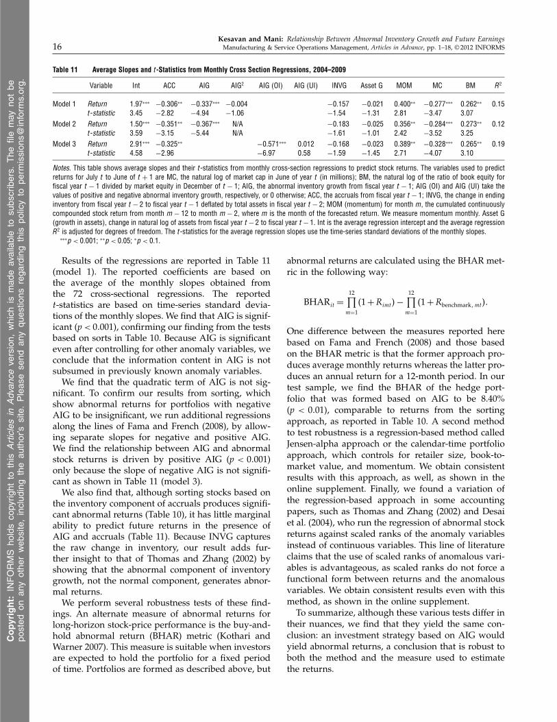
Kesavan and Mani: Relationship Between Abnormal Inventory Growth and Future Earnings16 Manufacturing & Service Operations Management, Articles in Advance, pp. 1–18, © 2012 INFORMS
Table 11 Average Slopes and t-Statistics from Monthly Cross Section Regressions, 2004–2009
Variable Int ACC AIG AIG2 AIG (OI) AIG (UI) INVG Asset G MOM MC BM R2
Model 1 Return 1097∗∗∗ −00306∗∗ −00337∗∗∗ −00004 −00157 −00021 00400∗∗ −00277∗∗∗ 00262∗∗ 0015t-statistic 3045 −2082 −4094 −1006 −1054 −1031 2081 −3047 3007
Model 2 Return 1050∗∗∗ −00351∗∗ −00367∗∗∗ N/A −00183 −00025 00356∗∗ −00284∗∗∗ 00273∗∗ 0012t-statistic 3059 −3015 −5044 N/A −1061 −1001 2042 −3052 3025
Model 3 Return 2091∗∗∗ −00325∗∗ −00571∗∗∗ 00012 −00168 −00023 00389∗∗ −00328∗∗∗ 00265∗∗ 0019t-statistic 4058 −2096 −6097 0058 −1059 −1045 2071 −4007 3010
Notes. This table shows average slopes and their t-statistics from monthly cross-section regressions to predict stock returns. The variables used to predictreturns for July t to June of t + 1 are MC, the natural log of market cap in June of year t (in millions); BM, the natural log of the ratio of book equity forfiscal year t − 1 divided by market equity in December of t − 1; AIG, the abnormal inventory growth from fiscal year t − 1; AIG (OI) and AIG (UI) take thevalues of positive and negative abnormal inventory growth, respectively, or 0 otherwise; ACC, the accruals from fiscal year t − 1; INVG, the change in endinginventory from fiscal year t − 2 to fiscal year t − 1 deflated by total assets in fiscal year t − 2; MOM (momentum) for month m, the cumulated continuouslycompounded stock return from month m − 12 to month m − 2, where m is the month of the forecasted return. We measure momentum monthly. Asset G(growth in assets), change in natural log of assets from fiscal year t − 2 to fiscal year t − 1. Int is the average regression intercept and the average regressionR2 is adjusted for degrees of freedom. The t-statistics for the average regression slopes use the time-series standard deviations of the monthly slopes.
∗∗∗p < 00001; ∗∗p < 0005; ∗p < 001.
Results of the regressions are reported in Table 11(model 1). The reported coefficients are based onthe average of the monthly slopes obtained fromthe 72 cross-sectional regressions. The reportedt-statistics are based on time-series standard devia-tions of the monthly slopes. We find that AIG is signif-icant (p < 00001), confirming our finding from the testsbased on sorts in Table 10. Because AIG is significanteven after controlling for other anomaly variables, weconclude that the information content in AIG is notsubsumed in previously known anomaly variables.
We find that the quadratic term of AIG is not sig-nificant. To confirm our results from sorting, whichshow abnormal returns for portfolios with negativeAIG to be insignificant, we run additional regressionsalong the lines of Fama and French (2008), by allow-ing separate slopes for negative and positive AIG.We find the relationship between AIG and abnormalstock returns is driven by positive AIG (p < 00001)only because the slope of negative AIG is not signifi-cant as shown in Table 11 (model 3).
We also find that, although sorting stocks based onthe inventory component of accruals produces signifi-cant abnormal returns (Table 10), it has little marginalability to predict future returns in the presence ofAIG and accruals (Table 11). Because INVG capturesthe raw change in inventory, our result adds fur-ther insight to that of Thomas and Zhang (2002) byshowing that the abnormal component of inventorygrowth, not the normal component, generates abnor-mal returns.
We perform several robustness tests of these find-ings. An alternate measure of abnormal returns forlong-horizon stock-price performance is the buy-and-hold abnormal return (BHAR) metric (Kothari andWarner 2007). This measure is suitable when investorsare expected to hold the portfolio for a fixed periodof time. Portfolios are formed as described above, but
abnormal returns are calculated using the BHAR met-ric in the following way:
BHARit =
12∏
m=1
41 +Rimt5−12∏
m=1
41 +Rbenchmark1mt50
One difference between the measures reported herebased on Fama and French (2008) and those basedon the BHAR metric is that the former approach pro-duces average monthly returns whereas the latter pro-duces an annual return for a 12-month period. In ourtest sample, we find the BHAR of the hedge port-folio that was formed based on AIG to be 8.40%(p < 0001), comparable to returns from the sortingapproach, as reported in Table 10. A second methodto test robustness is a regression-based method calledJensen-alpha approach or the calendar-time portfolioapproach, which controls for retailer size, book-to-market value, and momentum. We obtain consistentresults with this approach, as well, as shown in theonline supplement. Finally, we found a variation ofthe regression-based approach in some accountingpapers, such as Thomas and Zhang (2002) and Desaiet al. (2004), who run the regression of abnormal stockreturns against scaled ranks of the anomaly variablesinstead of continuous variables. This line of literatureclaims that the use of scaled ranks of anomalous vari-ables is advantageous, as scaled ranks do not force afunctional form between returns and the anomalousvariables. We obtain consistent results even with thismethod, as shown in the online supplement.
To summarize, although these various tests differ intheir nuances, we find that they yield the same con-clusion: an investment strategy based on AIG wouldyield abnormal returns, a conclusion that is robust toboth the method and the measure used to estimatethe returns.
Copyright:
INFORMS
holdsco
pyrig
htto
this
Articlesin
Adv
ance
version,
which
ismad
eav
ailableto
subs
cribers.
The
filemay
notbe
posted
onan
yothe
rweb
site,includ
ing
the
author’s
site.Pleas
ese
ndan
yqu
estio
nsrega
rding
this
policyto
perm
ission
s@inform
s.org.

Kesavan and Mani: Relationship Between Abnormal Inventory Growth and Future EarningsManufacturing & Service Operations Management, Articles in Advance, pp. 1–18, © 2012 INFORMS 17
8. Conclusion, Limitations, andFuture Work
This paper documents an inverted-U relationshipbetween abnormal inventory growth and one-year-ahead earnings for retailers, using publicly availablefinancial data. Thus, it demonstrates that the inverted-U relationship that forms the building block of inven-tory models at the SKU level can be detected atthe firm level as well. In addition, our paper showsthat Wall Street analysts and investors do not fullyincorporate the information in AIG in their earnings’forecasts and investment decisions, respectively. Byquantifying the anomalous stock market returns asso-ciated with AIG, our paper shows that a benchmark-ing metric derived from the operations managementliterature can serve as a basis for investment strategy.
Our paper does have limitations. First, our paperis limited to the retail sector. It would be interest-ing to examine other sectors to determine the valueof an inventory-based benchmarking metric froman investment stand point. Second, all the analysisreported in this paper are conducted at an annuallevel. Because annual inventory turns of retailers aretypically less than one, it is likely that the effects thatwe report are larger when observed in quarterly data.In fact, our longitudinal analysis with analysts’ fore-casts suggests that the bias predicted by AIG disap-pears six months after the release of 10-K statements.So, future research may perform quarterly analysisto examine if there is an improvement in the hedgeportfolio returns. Finally, future research may alsoconsider ways to improve the benchmarking modelfor retail used in this paper. An extension to themodel may consider including data on product vari-ety (Rajagopalan 2010) and competition (Olivares andCachon 2009) because they have been found to affectinventory levels of retailers. However, data for thesetwo variables are not available in the 10-K statements,so it may be necessary to look for other sources orviable proxies.
Future research may also examine the cause ofabnormal returns documented in our study. Theaccrual literature in accounting points to two possibleavenues of research. First, firms with abnormal inven-tory growth could have a different risk profile. Second,investors might be missing information contained inAIG, leading to a mispricing of these stocks. Knowl-edge of the underlying cause would enable us to deter-mine whether the abnormal returns associated withAIG would persist in equilibrium or if investors wouldarbitrage the anomalous returns away with time.
Electronic CompanionAn electronic companion to this paper is available aspart of the online version at http://dx.doi.org/10.1287/msom.1120.0389.
AcknowledgmentsThe authors thank Jeffery Abarbanell, Jennifer Conrad,Vinayak Deshpande, Vishal Gaur, Nandini Lahiri, AnanthRaman, Vinod Singhal, Bradley Staats, JayashankarSwaminathan, Mohan Venkatachalam; seminar participantsat the University of Chicago Booth School of Business,Duke University’s Fuqua School of Business, INSEAD, andSauder School of Business; the Equity Research Group atGoldman Sachs; and seminar participants at the 4th Empir-ical Research Workshop held at the Wharton School of theUniversity of Pennsylvania, 2009.
ReferencesAbarbanell JS, Bushee BJ (1997) Fundamental analysis, future earn-
ings, and stock prices. J. Accounting Res. 35(1):1–24.Aiken LS, West SG (1991) Multiple Regression: Testing and Interpreting
Interactions (Sage Publications, Newbury Park, CA).Allen EJ, Larson CR, Sloan RG (2011) Accrual reversals, earnings
and stock returns. Working paper, University of California,Berkeley, Berkeley.
Anderson EA, Fornell C, Mazvancheryl SK (2004) Customer satis-faction and shareholder value. J. Marketing 68(4):172–185.
Bernard VL, Noel J (1991) Do inventory disclosures predict salesand earnings? J. Accounting, Auditing, Finance 6(2):145–181.
Bernstein F, Federgruen A (2004) A general equilibrium modelfor industries with price and service competition. Oper. Res.52(6):868–886.
Bradshaw MT, Richardson SA, Sloan RG (2001) Do analystsand auditors use information in accruals? J. Accounting Res.39(1):45–74
Carpenter RE, Fazzri SM, Petersen BC (1998) Financing constraintsand inventory investment: A comparative study with high-frequency panel data. Rev. Econom. Statist. 80(4):513–519.
Chan K, Chan L, Jegadeesh N, Lakonishok J (2001) Earnings qualityand stock returns. J. Bus. 79(3):1041–1082.
Chen H, Murray FZ, Wu OQ (2007) U.S. retail and wholesaleinventory performance from 1981 to 2004. Manufacturing Ser-vice Oper. Management 9(4):430–456.
Dana J (2001) Competition in price and availability when availabil-ity is unobservable. RAND J. Econom. 32(4):497–513.
Desai H, Rajgopal S, Venkatachalam M (2004) Value glamourand accrual mispricing, one anomaly or two? Accounting Rev.79(2):355–385.
Durtschi C, Easton P (2005) Earnings management? The shapesof the frequency distributions of earnings metrics are not evi-dence ipso facto. J. Accounting Res. 43(4):557–592.
Ferguson M, Koenigsberg O (2007) How should a firm man-age deteriorating inventory? Production Oper. Management16(3):306–321.
Fisher M (1997) What is the right supply chain for your product?Harvard Bus. Rev. 77(2):105–116.
Fama EF, French KR (2008) Dissecting anomalies. J. Finance63(4):1653–1678.
Fama E, MacBeth J (1973) Risk, return, and equilibrium: Empiricaltests. J. Political Econom. 81(3):607–636.
Gallego G, van Ryzin G (1994) Optimal dynamic pricing of inven-tories with stochastic demand. Management Sci. 40(8):999–1020.
Gaur V, Kesavan S (2009) The effects of firm size and sales growthrate on inventory turnover performance in the U.S. retail sec-tor. Agrawal N, Smith S, eds. Retail Supply Chain Management(Springer Science+Business Media, New York), 25–52.
Gaur V, Park Y (2007) Asymmetric consumer learning and inven-tory competition. Management Sci. 53(2):227–240.
Copyright:
INFORMS
holdsco
pyrig
htto
this
Articlesin
Adv
ance
version,
which
ismad
eav
ailableto
subs
cribers.
The
filemay
notbe
posted
onan
yothe
rweb
site,includ
ing
the
author’s
site.Pleas
ese
ndan
yqu
estio
nsrega
rding
this
policyto
perm
ission
s@inform
s.org.

Kesavan and Mani: Relationship Between Abnormal Inventory Growth and Future Earnings18 Manufacturing & Service Operations Management, Articles in Advance, pp. 1–18, © 2012 INFORMS
Gaur V, Fisher ML, Raman A (2005) An econometric analysis ofinventory turnover performance in retail services. ManagementSci. 51(2):181–194.
Givoly D, Lakonishok J (1984) The quality of analysts’ forecasts ofearnings. Financial Anal. J. 40(5):40–47.
Gu Z, Wu J (2003) Earnings skewness and analyst forecast bias.J. Accounting Econom. 35(1):5–29.
Hendricks KB, Singhal VR (2005) Association between supplychain glitches and operating performance. Management Sci.51(5):695–711.
Hendricks KB, Singhal VR (2009) Demand–supply mismatchesand stock market reaction: Evidence from excess inven-tory announcement. Manufacturing Service Oper. Management11(3):509–524.
Hribar P, Collins D (2002) Errors in estimating accruals. J. Account-ing Res. 40(1):105–134.
Ittner CD, Larcker DF (1998) Are nonfinancial measures leadingindicators of financial performance? An analysis of customersatisfaction. J. Accounting Res. 36(3):1–35.
Jegadeesh N (1990) Evidence of predictable behavior of securityreturns. J. Finance 45(3):881–898.
Kesavan S, Gaur V, Raman A (2010) Do inventory and gross margindata improve sales forecasts for U.S. public retailers? Manage-ment Sci. 56(9):1519–1533.
Kothari SP, Warner JB (2007) Econometrics of event studies. EckboBE, ed. Handbook of Corporate Finance: Empirical CorporateFinance (Elsevier, North Holland), 3–36.
Lintner J (1965) The valuation of risk assets and the selection ofrisky investments in stock portfolios and capital budgets. Rev.Econom. Statist. 47(1):13–37.
Maddala GS (2001) Introduction to Econometrics (John Wiley & Sons,New York).
Olivares M, Cachon GP (2009) Competing retailers and inventory:An empirical investigation of General Motors’ dealerships inisolated U.S. markets. Management Sci. 55(9):1586–1604.
Rajagopalan S (2010) Factors driving inventory levels at US retail-ers. Working paper, University of Southern California, LosAngeles.
Rumyantsev S, Netessine S (2007a) What can be learned from clas-sical inventory models? A cross-industry exploratory investi-gation. Manufacturing Service Oper. Management 9(4):409–429.
Rumyantsev S, Netessine S (2007b) Should inventory policy be leanor responsive? Evidence for US public companies. Workingpaper, INSEAD, Fontainebleau, France.
Sharpe WF (1964) Capital asset prices: A theory of market equilib-rium under conditions of risk. J. Finance 19(3):425–442.
Sloan R (1996) Do stock prices fully reflect information in accru-als and cash flows about future earnings? Accounting Rev.71(3):289–315.
Smith S, Achabal D (1998) Clearance pricing and inventory policiesfor retail chains. Management Sci. 44(3):285–300.
Thomas JK, Zhang H (2002) Inventory changes and future returns.Rev. Accounting Stud. 7(2):163–187.
Zach T (2003) Inside the “accrual anomaly.” Working paper,Washington University in St. Louis, St. Louis.
Copyright:
INFORMS
holdsco
pyrig
htto
this
Articlesin
Adv
ance
version,
which
ismad
eav
ailableto
subs
cribers.
The
filemay
notbe
posted
onan
yothe
rweb
site,includ
ing
the
author’s
site.Pleas
ese
ndan
yqu
estio
nsrega
rding
this
policyto
perm
ission
s@inform
s.org.