Open Journal of Accounting, 2018, 7, 159-180 http://www.scirp.org/journal/ojacct

ISSN Online: 2169-3412 ISSN Print: 2169-3404

DOI: 10.4236/ojacct.2018.72011 Apr. 12, 2018 159 Open Journal of Accounting

The Recognition of the Asymmetry: Sticky Costs and Cognitive Biases

Nicola Dalla Via

RSM Erasmus University, Rotterdam, Netherlands

Abstract This paper investigates whether individuals are accurate in recognizing and predicting cost stickiness under different presentation formats. In particular, I conduct an experiment manipulating the degree of cost asymmetry (non-sticky, semisticky, sticky), which is the cost behavior when revenues increase or decrease, and the presentation of financial information (monetary amounts vs. percentages). Contrary to the expectation, participants are more likely to recognize and predict accurately sticky costs rather than nonsticky costs (i.e. cost symmetry). They mentally apply a sticky model also to predict changes of nonsticky costs. Moreover, the presentation of variations expressed as per-centages allows more accurate forecasts. Further, a significant interaction ef-fect between the two manipulations is found. The cognitive ability and the cognitive style of the participants are measured in order to disentangle possi-ble confounding effects. The findings of this study suggest that the mental models of the individuals and their cognitive biases influence cost forecasts and adjustments decisions.

Keywords Sticky Costs, Mental Models, Lens Model, Framing, Linearity

1. Introduction

The diffusion of new management accounting techniques and the spread of in-formation technology systems like Enterprise Resource Planning (ERP) systems increased the availability of timely and accurate financial reports for managerial decision making such as cost management choices. The adjustment of resources in response to changes in sales volume is a primary issue managed in an organi-zation. Anderson et al. (2003) explicitly investigated the asymmetric behavior of costs when volume increases or decreases [1]. They call sticky this kind of costs

How to cite this paper: Dalla Via, N. (2018) The Recognition of the Asymmetry: Sticky Costs and Cognitive Biases. Open Journal of Accounting, 7, 159-180. https://doi.org/10.4236/ojacct.2018.72011 Received: February 26, 2018 Accepted: April 9, 2018 Published: April 12, 2018 Copyright © 2018 by author and Scientific Research Publishing Inc. This work is licensed under the Creative Commons Attribution International License (CC BY 4.0). http://creativecommons.org/licenses/by/4.0/

Open Access

N. Dalla Via

DOI: 10.4236/ojacct.2018.72011 160 Open Journal of Accounting

and propose an alternative model of cost behavior based on deliberate adjust-ments by managers. However, several studies provide evidence that managers prefer to use their subjectivity instead of statistical computations when a fast and cheap decision process is required [2] [3]. In addition to the benefits of making judgments using subjective analysis, issues of accuracy emerge when individuals mentally represent the relationships among variables. The cognitive modeling by managers is also influenced by the layout of financial reports and by the framing of information which are different across organization [4] [5] [6] [7]. The pres-entation of reports with the same information content but different format re-sults in different decisions. Overall, psychological determinants influence the cognition of the managers and hence the accuracy of their decision outcomes.

In this study I examine how variations in the degree of cost asymmetry (i.e. nonsticky, semisticky, sticky) and in the presentation format of financial infor-mation (i.e. monetary amounts or percentages) influence the accuracy of indi-vidual cost predictions. I expect that the accuracy in recognizing and predicting changes in the level of costs is higher when they are symmetric rather than sticky. Moreover, I expect that, with the same information content, the predic-tion is more accurate when percentages variations are provided compared to monetary amounts. I further expect an interaction of the two variables such that an increase in accuracy due to the symmetric behavior of costs is more pro-nounced when financial information is exhibited as absolute amounts than per-centages.

I conduct a laboratory experiment with a 3 × 2 design mixing a with-in-subjects condition with a between-subjects condition. I manipulate the degree of cost stickiness and the format of the financial information. The experimental task required the participants to mentally identify the relationship between rev-enues and costs and then to predict the trend of costs accordingly.

This study contributes to the literature in several ways. First, I extend the lite-rature on cost stickiness by adopting both a different level of analysis (i.e. indi-vidual) and a different methodology (i.e. laboratory experiment) compared to the majority of the studies. To my knowledge, only Banker et al. (2014) consi-dered determinants pertaining to individual features of the managers such as optimism and pessimism [8]. Second, I show that the presentation of informa-tion with the same content, but presented in different format, influences the outcome of the decision. These findings add new knowledge to the literature in behavioral accounting that examines the impact of information organization and presentation on decision making. Third, I enlarge the small number of manage-ment accounting studies focused on understanding the cognitive processes un-derlying judgments and decision making [9] [10]. Further, I consider also the cognitive ability and the cognitive style of individuals in order to understand whether specific cognitive features impact subjects’ mental models.

The findings of this work have important managerial implications. Companies should consider that an inappropriate preparation of financial reports leads to

N. Dalla Via

DOI: 10.4236/ojacct.2018.72011 161 Open Journal of Accounting

qbiases and inaccurate judgments. Moreover, when timely decisions are re-quired, various aspects have to be considered both at a cognitive and at analyti-cal level.

The remainder of the paper is organized as follows. Section 2 examines the re-levant literature and the development of the hypotheses. Section 3 provides a description of the experimental method and Section 4 presents the results. Sec-tion 5 concludes.

2. Literature Review and Hypothesis Development 2.1. Literature Review

During the last decade the topic of cost stickiness gained importance in the ac-counting literature. Anderson et al. (2003) proposed an alternative model of cost behavior in which they contrast the deliberate adjustments of resources by managers in response to changes in volume with the mechanistic movement of costs [1]. The earlier results of sticky behavior of costs were confirmed and ex-tended in the following years by several studies. However, a recent debate about the appropriateness and generalizability of the findings appeared in the literature with, on the one hand, the critical works of Anderson and Lanen (2009) [11] and Balakrishnan et al. (2014) [12], and on the other hand Banker et al. (2011) [13] defending the position of Anderson et al. (2003) [1] and their followers. The fo-cus of the empirical tests on cost stickiness has been conducted on firm-specific determinants [1] or on economy-wide forces [14]. Only recently Banker et al. (2014) [8] considered determinants pertaining to individual features of the managers such as optimism and pessimism. However, they measured the atti-tude using financial data, and in particular according to prior period sales. A de-cline in sales from the previous period, or the prior two periods, is a proxy for pessimism, whereas an increasing trend is considered a proxy for optimism. These findings suggest that the individual behavior and the subjective judgments have a role in cost adjustments decisions.

More in general, in managerial decision making involving cost accounting data, the manager has to draw inferences from the available data in order to make judgments and take actions. Subjective analysis provides a more timely de-cision process, but the accuracy of the judgment can differ depending on the re-lation underlying the variables. This is due to variations in the individual mental representation and it results in different outcomes across subjects [2] [3]. Studies about multiple-cue probability learning showed that differences in the form of the function have an impact upon the achievement by the subjects. In particular, linear relations are learned better than nonlinear relations and faster when they are positive compared to negative. The linear portion is also better captured when the request is to learn an inverted U-shaped relation compared to a U-shaped relation [15] [16].

Further, the manager has to draw inferences about the relation starting from accounting data which are normally provided as absolute numbers. The ability

N. Dalla Via

DOI: 10.4236/ojacct.2018.72011 162 Open Journal of Accounting

to work with percentages and ratios is required to find a percent increase or de-crease of one number on another and then apply the percentage to find the re-sult of a percent increase or decrease on a given number [17] [18]. The difficul-ties encountered in computational task, such as processing percentage informa-tion, are other important issues affecting the inference of the appropriate ac-counting relation [19] [20]. Mental techniques used to solve complex arithmetic and the use of calculation anchors can lead to non-accurate predictions and to failures in the recognition of the asymmetry between increasing and decreasing percentages [21] [22] [23]. The cognitive ability of the subjects has to be con-trolled in order to disentangle the effects due to different skills from the cogni-tive biases. In particular the ability to understand and use numeric information is called numeracy and its measure has been used in different contexts [24] [25]. Another interesting determinant used in decision making but not in the ac-counting field is the decision style adopted by the individual. A deeper under-standing of the way of thinking and of processing information provides useful indication about the inferences made about the data. The distinction between individuals with a predominant intuitive cognitive style, more prone to emphas-ize feelings and global perspective, and individuals with a predominant analyti-cal style, more focused on mental reasoning and details, leads to different find-ings about mental models and prediction accuracy. These two ways of processing information correspond also to the distinction between System 1 and System 2 introduced by Stanovich and West (2000) [26] and proposed by the dual-process theory which argue the presence of “two minds in one brain” ([27], p.458).

2.2. Hypothesis Development

All the studies on cost stickiness model the relation between revenues, used as a proxy for the sales volume, and costs as a linear function. In particular, the slope is higher when the sales volume registers an increase rather than a decrease. The psychological literature on multiple-cue probability learning showed that linear relations are learned better than nonlinear relations [15] [16] and that the esti-mations are more accurate when positive relations are involved compared to negative relations [28] [29]. In my experiment the condition with symmetric changes in costs is referable to a perfect linear relation. The exhibition of a de-gree of asymmetry, firstly low and then more pronounced, introduces a noise in the linearity. I expect that the change of slope in the negative domain is not no-ticed by the majority of individuals because they derive inferences from the posi-tive side, which is cognitively more understandable, but constant across condi-tions. According to these considerations, I predict that individuals subjectively recognize and estimate more accurately symmetric changes in costs rather than sticky variations. Therefore, my first hypothesis is formulated as follows.

Hypothesis 1: Judgments are more accurate when costs change symmetrically in case of increase or decrease rather than with a sticky behavior.

In addition to the degree of asymmetry, I introduce a change in the presenta-

N. Dalla Via

DOI: 10.4236/ojacct.2018.72011 163 Open Journal of Accounting

tion format of the financial information. Financial reports are expressed both using monetary amounts and percentages. The computation of forecasts draw-ing from absolute monetary amounts requires certain mental ability and effort. First, the individual has to derive the percentage change and then apply the re-sult to a given number. However, when percentages are directly provided, the cognitive load is reduced and the effort is limited to the understanding of the re-lation between variables. According to the different cognitive load requested to individuals, I expect more accurate judgments when data are showed as percen-tages rather than absolute monetary amounts. Accordingly, I formulate the fol-lowing hypothesis.

Hypothesis 2: Judgments are more accurate when data are presented in per-centages rather than monetary amounts.

Finally, I expect an interaction between the degree of cost asymmetry and the presentation format of the financial information. The recognition of asymmetric changes in costs requires a more careful study of the whole cues in order to un-derstand the presence of a change of slope between increases and decreases in revenues and as a consequence in costs, but also the magnitude of such a change. It is in this condition that the display of percentages instead of monetary amounts allows to derive more accurate inferences from the data. However, the gain in accuracy across different degrees of symmetry, from the lowest to the highest, is higher with monetary amounts than percentages. These considera-tions are summarized in the following hypothesis.

Hypothesis 3: The presentation of data in percentages rather than monetary amounts is more beneficial under cost stickiness compared to cost symmetry.

3. Experimental Method 3.1. Research Design and Participants

To test the hypotheses I conducted a laboratory experiment with a 3 × 2 design mixing a within-subjects treatment with a between-subjects treatment. The first manipulation, conducted within-subjects, is the degree of cost asymmetry (i.e. nonsticky, semisticky, sticky). The highest degree of asymmetry corresponds to the sticky behavior of costs, whereas the nonsticky case is the one involving symmetric changes. The second manipulation, conducted between-subjects, is the presentation format (i.e. monetary amounts vs. percentages).

The experiment was conducted at the Cognitive and Experimental Economics Laboratory of an Italian university using the software z-Tree [30]. I ran four separate sessions, two for each between-subjects treatment. The subjects are 78 undergraduate students who participated in a voluntary way registering for the experiments in the laboratory web-site after an e-mail announcement sent to the entire mailing-list. Four sessions were run and 38 subjects were assigned to the absolute values conditions (18 + 20) and 40 to the percentages condition (20 + 20). The age of the participants ranges from 19 to 37, with a mean of 22.76 years. There are 43 males (55.1%) and 35 females (44.9%). Participants received a

N. Dalla Via

DOI: 10.4236/ojacct.2018.72011 164 Open Journal of Accounting

show-up fee of 3 euro and a variable pay of maximum 10 euro computed accor-dingly to the accuracy of their judgments as explained below. The average earn-ing is 10.50 Euro. The experiment took, on average, about one hour and fifteen minutes to be completed.

3.2. Setting and Task

In the experiment, participants assumed the role of CFO of an important hotel chain owner of 20 hotels of different dimensions, but common target of custom-ers. They are instructed that all the hotels are organized similarly, with the same control system and they strictly follow the rules and the procedures imposed by the top management of the controlling company. The story describes an acquisi-tion from a competitor of other 20 hotels. During 2011, the year of the acquisi-tion, the control system of the new hotels is replaced with the one adopted by the other hotels of the group as well as the organizational procedures. At the begin-ning of 2012 the whole chain, composed now by 40 hotels, adopts the same sys-tem and the same rules.

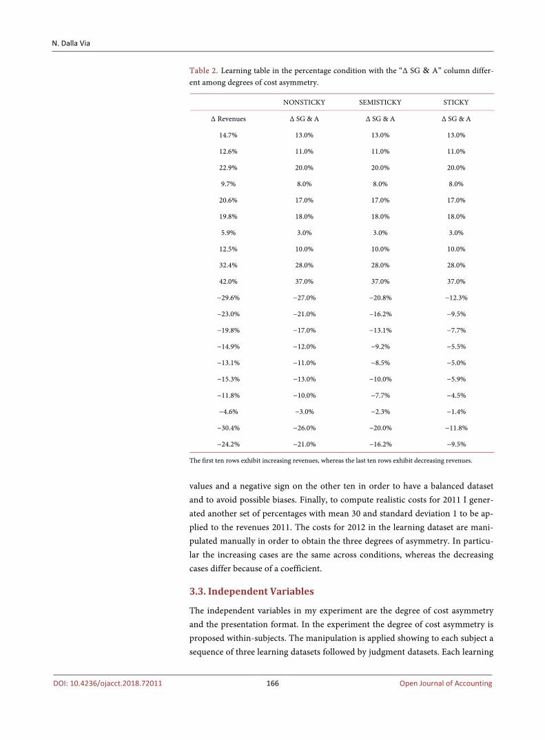
Participants received data about revenues and selling, general and administra-tive (SG & A) expenses registered in 2011 for the 20 “historical” hotels. I keep the task as simple as possible explaining that there is an underlying relationship between changes in revenues and changes in SG & A costs.I use SG & A costs to be consistent with the majority of the literature on cost stickiness (e.g. Anderson et al., 2003). In the same table, figures for both variables are also presented as forecasts for 2012. The table is called in my experiment the learning dataset (Table 1 and Table 2). More in detail, the two tables exhibit financial informa-tion related to the hotels owned by the hotel chain. Table 1 presents revenues and SG & A costs as monetary amounts with reference to year 2011 and 2012. Table 2 presents revenues and SG & A costs as percentage change from year 2011 to 2012. In both tables, the first ten rows exhibit increasing revenues, whe-reas the last ten rows exhibit decreasing revenues. Participants in the monetary amount condition examined the data presented in Table 1, whereas participants in the percentage condition examined the data presented in Table 2. Further, the last three columns of Table 1 and Table 2 differ per experimental condition. Depending on the degree of cost asymmetry condition (i.e. nonsticky, semis-ticky, sticky), only one of the last three columns is showed to the participants.

After an accurate study of the learning dataset, the participants received a similar table with financial data referred to the 20 new hotels acquired. I call this table the judgment dataset (Table 3 and Table 4).

More in detail, the two tables exhibit financial information related to the newly acquired hotels. Table 3 presents revenues as monetary amounts with reference to year 2011 and 2012 and SG & A costs with reference to year 2011. Table 4 presents revenues as percentage change from year 2011 to 2012. In both tables, the first ten rows exhibit increasing revenues, whereas the last ten rows exhibit decreasing revenues. Participants in the monetary amount condition

N. Dalla Via

DOI: 10.4236/ojacct.2018.72011 165 Open Journal of Accounting

Table 1. Learning table in the monetary amounts condition with the “SG & A 2012” column different among degrees of cost asymmetry.

NONSTICKY SEMISTICKY STICKY

Revenues 2011 Revenues 2012 SG & A 2011 SG & A 2012 SG & A 2012 SG & A 2012

4,458,068 5,111,945 1,324,811 1,497,037 1,497,037 1,497,037

6,044,167 6,803,174 1,809,650 2,008,711 2,008,711 2,008,711

5,995,573 7,370,229 1,647,235 1,976,681 1,976,681 1,976,681

5,709,550 6,263,147 1,621,388 1,751,099 1,751,099 1,751,099

3,858,806 4,652,470 1,215,675 1,422,339 1,422,339 1,422,339

3,141,165 3,764,406 914,017 1,078,539 1,078,539 1,078,539

6,819,873 7,220,775 2,094,389 2,157,221 2,157,221 2,157,221

4,282,893 4,819,702 1,264,976 1,391,474 1,391,474 1,391,474

5,325,361 7,048,718 1,655,942 2,119,605 2,119,605 2,119,605

5,617,829 7,977,260 1,663,003 2,278,314 2,278,314 2,278,314

5,306,875 3,734,729 1,639,897 1,197,125 1,299,303 1,438,637

4,797,335 3,696,246 1,498,805 1,184,056 1,256,691 1,355,738

2,810,185 2,252,841 819,507 680,191 712,340 756,181

2,651,448 2,257,414 751,559 661,372 682,184 710,565

5,142,303 4,467,270 1,547,185 1,376,995 1,416,270 1,469,826

6,272,465 5,315,819 1,912,681 1,664,032 1,721,413 1,799,659

6,536,288 5,767,096 1,906,517 1,715,865 1,759,862 1,819,857

5,908,571 5,636,770 1,751,349 1,698,809 1,710,934 1,727,467

5,270,284 3,667,537 1,533,888 1,135,077 1,227,111 1,352,611

3,394,624 2,572,108 1,059,655 837,128 888,480 958,506

The first ten rows exhibit increasing revenues, whereas the last ten rows exhibit decreasing revenues.

received the data presented in Table 3, whereas participants in the percentage condition received the data presented in Table 4. The only notable difference with the learning table is that the column containing the costs forecasts for 2012 (or the expected percentage variation in the percentage condition) is blank. Thus, participants had to fill in the last column of Table 3 or Table 4. The learning table is always present on the screen together with the judgment table consistently with the availability of past data in companies.

The data used in the learning dataset and in the judgment dataset were drawn from a normal distribution with a given mean and standard deviation. In partic-ular, revenues for 2011 were drawn from a normal with mean 5 million and standard deviation 1,250,000. Then I generated a set of percentages with mean 20 and standard deviation 10 to compute realistic growth or declines for the revenues of 2012 starting from the amounts 2011. I forced a positive sign on ten

N. Dalla Via

DOI: 10.4236/ojacct.2018.72011 166 Open Journal of Accounting

Table 2. Learning table in the percentage condition with the “Δ SG & A” column differ-ent among degrees of cost asymmetry.

NONSTICKY SEMISTICKY STICKY

Δ Revenues Δ SG & A Δ SG & A Δ SG & A

14.7% 13.0% 13.0% 13.0%

12.6% 11.0% 11.0% 11.0%

22.9% 20.0% 20.0% 20.0%

9.7% 8.0% 8.0% 8.0%

20.6% 17.0% 17.0% 17.0%

19.8% 18.0% 18.0% 18.0%

5.9% 3.0% 3.0% 3.0%

12.5% 10.0% 10.0% 10.0%

32.4% 28.0% 28.0% 28.0%

42.0% 37.0% 37.0% 37.0%

−29.6% −27.0% −20.8% −12.3%

−23.0% −21.0% −16.2% −9.5%

−19.8% −17.0% −13.1% −7.7%

−14.9% −12.0% −9.2% −5.5%

−13.1% −11.0% −8.5% −5.0%

−15.3% −13.0% −10.0% −5.9%

−11.8% −10.0% −7.7% −4.5%

−4.6% −3.0% −2.3% −1.4%

−30.4% −26.0% −20.0% −11.8%

−24.2% −21.0% −16.2% −9.5%

The first ten rows exhibit increasing revenues, whereas the last ten rows exhibit decreasing revenues.

values and a negative sign on the other ten in order to have a balanced dataset and to avoid possible biases. Finally, to compute realistic costs for 2011 I gener-ated another set of percentages with mean 30 and standard deviation 1 to be ap-plied to the revenues 2011. The costs for 2012 in the learning dataset are mani-pulated manually in order to obtain the three degrees of asymmetry. In particu-lar the increasing cases are the same across conditions, whereas the decreasing cases differ because of a coefficient.

3.3. Independent Variables

The independent variables in my experiment are the degree of cost asymmetry and the presentation format. In the experiment the degree of cost asymmetry is proposed within-subjects. The manipulation is applied showing to each subject a sequence of three learning datasets followed by judgment datasets. Each learning

N. Dalla Via

DOI: 10.4236/ojacct.2018.72011 167 Open Journal of Accounting

Table 3. Judgment table in the monetary amounts condition.

Revenues 2011 Revenues 2012 SG & A 2011 SG & A 2012

3,602,371 4,053,686 1,095,184

4,461,330 5,166,557 1,274,505

4,799,706 5,798,850 1,448,979

6,088,324 6,437,228 1,788,799

6,215,933 7,285,956 1,830,599

4,647,736 5,067,036 1,366,648

6,974,771 9,014,606 2,043,479

2,616,379 3,046,808 824,792

5,095,946 6,058,950 1,556,334

5,448,454 6,547,880 1,685,546

5,089,234 3,626,536 1,491,644

4,216,785 3,070,688 1,292,395

3,739,614 2,424,073 1,069,309

5,556,302 3,943,205 1,664,435

4,494,544 2,438,825 1,341,145

5,101,892 4,921,011 1,554,345

5,652,328 4,797,321 1,765,266

5,608,013 4,332,177 1,670,867

4,897,049 4,184,675 1,371,066

1,516,740 1,298,528 413,832

The first ten rows exhibit increasing revenues, whereas the last ten rows exhibit decreasing revenues.

dataset differs by the 10 values of SG & A costs for 2012 decreased from 2011. The story provided to the participants explains that they have to analyze three different scenarios. The order of the rows in the tables and the order of the con-ditions is completely randomized in order to avoid confounding effects.

The presentation format is manipulated between-subjects. Half participants receive the tables with monetary amounts for 2011 and 2012, whereas the other half receives the same values computed as percentage changes between 2011 and 2012. The information content is constant because the underlying amounts are the same, but the presentation is different.

3.4. Procedure

Upon arrival, participants were randomly seated in the laboratory, each one in front of a computer. They were not able to communicate each other or to see the screens of other participants. The instructions were provided on paper and read aloud by one of the researchers present in the room. Moreover, they were not allowed to use calculators, computer programs, or to take notes during the expe-riment.

N. Dalla Via

DOI: 10.4236/ojacct.2018.72011 168 Open Journal of Accounting

Table 4. Judgment table in the percentage condition.

Δ Revenues Δ SG & A

12.5%

15.8%

20.8%

5.7%

17.2%

9.0%

29.2%

16.5%

18.9%

20.2%

−28.7%

−27.2%

−35.2%

−29.0%

−45.7%

−3.5%

−15.1%

−22.8%

−14.5%

−14.4%

The first ten rows exhibit increasing revenues, whereas the last ten rows exhibit decreasing revenues.

At the beginning participants received clear information about their compen-

sation. In addition to the show up fee they received a variable cash payment of maximum 10 euro related to the accuracy of their judgments. One of the three judgment tables completed by each participant is randomly extracted for the payment. The computation is made using a quadratic loss function (Equation (1)) in which the 20 predictive judgments are compared to the estimations computed using the Ordinary Least Squares (OLS) model underlying the learn-ing dataset. The formula is the following:

( )2Accuracy Score prediction of the participant OLS prediction= −∑ (1)

The highest is the accuracy score the lowest is the accuracy. The individual with the highest score receives a variable pay equal to zero and the other partici-pants receive a payment linearly and inversely related to the score.

The first screen of the experiment shows a comprehension check. The ques-tions have the purpose to check the correct comprehension of the instructions and of the task. The participants have to answer all the questions correctly in

N. Dalla Via

DOI: 10.4236/ojacct.2018.72011 169 Open Journal of Accounting

order to be able to proceed with the experiment. In the central part of the experiment, participants examine the learning table

for few minutes. When they believe that they have mentally identified the rela-tion between revenues and costs they can move to the judgment dataset in order to apply the model to the new data. They have to repeat the same procedure for the three scenarios.

In the final part of the experiment participants have to answer to a series of questions in order to capture their cognitive ability and style. All the participants are informed that the questions do not count for the compensation. The mathe-matical ability of the participants and their cognitive style are measured using instruments available in the literature. The original scale used to assess numera-cy is composed by three items [31], but I apply an expanded scale composed by 11 items [32]. The cognitive style is measured using an index (CSI) developed by Allinson and Hayes (1996) and constructed using 38 propositions with three possible answers (true, uncertain, false) [33]. The total rating of the individual identifies the intuitive (i.e. “right brain” thinking) or analytical (i.e. “left brain” thinking) orientation. The instrument has been used in several studies and its validity has been confirmed [34]. The distinction between the two types of cog-nitive processes is captured also with the last set of questions based on the Cog-nitive Reflection Test (CRT) developed by Frederick (2005) [35].

The experiment is concluded with a demographic questionnaire and the sub-sequent cash payment of the compensation. The final questionnaire included questions about gender, age, level of education, and work experience.

3.5. Dependent Variables

In this experiment, I use a linear regression to model the cognitive processes of the individuals. The most common model employed for this purpose is the lens model [36]. In the management accounting field this approach has been used to study accounting fixation [9], to examine the cognitive effects of the nonlineari-ties of cost and profit drivers [10], and also applied to archival data about inves-tors’ sophistication [37]. Figure 1 shows a visual representation of the lens mod-el. As indicated in Figure 1, the model provides several statistics used to study how information is processed from cues to predict outcomes. Examples are en-vironmental predictability, matching index, and response linearity. It is possible to compare the environmental model, obtained by regressing the actual out-comes on the information cues (left-hand side of Figure 1), with the estimations obtained for the policy-capturing models of each participant, obtained by re-gressing the individual’s judgments on the information cues (right-hand side of Figure 1). However, even if the model is widely used, some caution needs to be used in the interpretation of the results [38].

The regression model is the one used by Anderson et al. (2003) [1] and by the majority of the following studies on cost stickiness. The model is reported in Equation (2).

N. Dalla Via

DOI: 10.4236/ojacct.2018.72011 170 Open Journal of Accounting

Figure 1. Diagram of the lens model (see [39] for additional details).

,2012 ,20120 1

,2011 ,2011

,20122 ,

,2011

COST Revenuelog log

COST Revenue

RevenueDummy log

Revenue

i i

i i

ii i t

i

β β

β ε

= + ⋅

+ ⋅ ⋅ +

(2)

The stickiness behavior is isolated by the dummy variable, which takes the value “1” when revenues of the current period are decreased from the previous period and the value “0” in the opposite case. The measures computed by the lens model are useful to estimate the accuracy of the participants. The main sta-tistics are: environmental predictability, matching index, and response linearity. The first measure is not considered in my setting given that cannot be influenced by the task. The matching index is the correlation between the predictions ob-tained with the environmental model and the participant’s model. The response linearity (consistency) is a measure of consistency and it is computed as the cor-relation between the individual prediction and the estimation obtained using the policy-capturing model. The two variables are the main dependent variables of the experiment. A measure of judgment accuracy is also obtained with the product of matching and response linearity. According to Farrell et al. (2007) [10] it is also possible to compute a measure of judgment accuracy at mul-ti-person level called consensus, which is the degree of similarity among indi-vidual errors. The measure is computed as the correlation between a partici-pant’s prediction and the prediction for each of the other participants.

In addition to the dependent variables provided by the lens model I adopt another measure of judgment accuracy as in Luft and Shields (2001) [9]. The va-riable, called accuracy, is computed for each participant as the mean absolute

N. Dalla Via

DOI: 10.4236/ojacct.2018.72011 171 Open Journal of Accounting

error of the individual’s predictions (Equation (3)). The formula is the following: 20

1Accuracy20

pi eiiY Y

=−

=∑ (3)

where: Ypi: individual cost prediction for the i hotel Yei: actual cost for the i hotel In the presentation format with absolute values the variable accuracy is com-

puted equivalently both in Euro and percentages in order to facilitate the com-parison with the percentages format.

4. Results

I used Stata 12 and R to examine the experimental data and to conduct the em-pirical tests. The analysis of the manipulation check questions reveals that the participants in the absolute values condition perceive the task as more difficult than the participants in the percentages condition (p-value < 0.05). Moreover, the provided information is considered complete enough by the participants in the percentages condition and less complete by the participants in the absolute values condition (p-value < 0.05). Overall, the manipulation check is considered satisfactory.

The main hypotheses test is performed using a repeated-measures ANCOVA with the mean absolute error of the individual’s predictions (i.e. accuracy) as dependent variable. The two experimental conditions are the factors of the mod-el. In particular the presentation format is the between-subjects factor and the degree of asymmetry is the within-subjects factor. The interaction between the two conditions is also tested as within-subjects factor. Four categorical variables are included in the model as covariates: SEX, YDEGREE, NUMERACY, and CSI. SEX is a dummy variable indicating the gender of the participant (1 = male; 2 = female), YDEGREE indicates the academic year of enrolment (from 1 to 5), NUMERACY is the measure of mathematical ability (1 = high skills, numeracy above 7; 2 = low skills, numeracy below 7), and CSI is the indicator of cognitive style (1 = reflective and analytical, CSI above 38; 2 = intuitive, CSI below 38).

The results of the ANCOVA, exposed in Table 5, shows that the main effects of presentation format and degree of asymmetry are significant (F = 114.90, p < 0.01, and F = 7.77, p < 0.01, respectively) as well as the interaction between the two factors (F = 11.84, p < 0.01). These results appear to support the hypotheses. However, a full interpretation of these effects requires a more detailed explora-tion.

In combination with the ANCOVA presented in Table 5, the comparison of the judgment accuracy in Table 6 specifies better the findings and verifies the hypotheses. In the absolute values condition judgment accuracy is higher when the data exhibit a semisticky behavior compared to the nonsticky condition (mean absolute error is 143,565 vs. 228,317, respectively) or a sticky behavior compared to the nonsticky condition (139,025 vs. 228,317, respectively). These

N. Dalla Via

DOI: 10.4236/ojacct.2018.72011 172 Open Journal of Accounting

Table 5. Repeated measures ANCOVA with Accuracy as dependent variable.

Variable SS df MS F p-value

(two-tailed)

Covariates

Sex 0.0042 1 0.0042 0.91 0.34

Ydegree 0.0351 4 0.0088 1.88 0.12

Numeracy 0.0209 1 0.0209 4.48 0.04**

CSI 0.0025 1 0.0025 0.53 0.47

Between Subjects

Format 0.5369 1 0.5369 114.90 0.00***

Error 0.3224 69 0.0047

Within Subjects

Asymmetry 0.0415 2 0.0207 7.77 0.00***

Asymmetry x Format 0.0632 2 0.0316 11.84 0.00***

Error 0.4060 152 0.0027

Model: R2 = 0.72, Adjusted R2 = 0.58 ***, **, and * indicate statistical significance at the 1%, 5%, and 10% levels, respectively (two-tailed).

two comparisons are statistically significant (t-value = 2.78, p < 0.01 and t-value = 2.94, p < 0.001) and are in contrast with the effect predicted in hypothesis 1. Further, in the percentages condition the level of accuracy is not different across degrees of asymmetry. Overall, the results about the judgment accuracy values (i.e. mean absolute error) are the opposite of the expectation of hypothesis 1. Judgments are more accurate when costs exhibit sticky behavior instead of symmetrical changes when values are presented as monetary amounts. The par-ticipants denote a tendency to constantly use a mental model closer to the sticky behavior instead of a linear model with a constant slope in case of increasing or decreasing amounts. Despite the contrast with the expectation, the result is ex-tremely interesting because it confirms the importance of the individual level of analysis in the studies of cost stickiness.

The second part of Panel A in Table 6 compares the accuracy measured in the absolute values format with the accuracy in the percentages format. The mean absolute error is significantly lower in the percentages format in all the three de-grees of asymmetry than the monetary format. More in detail, in the non sticky condition, the mean absolute error is 0.163 in the absolute values condition and 0.019 in the percentages condition. The difference is statistically significant (t-value = 7.10, p-value < 0.001). The pattern is similar in the semisticky condi-tion (mean absolute error 0.102 vs. 0.025, t-value = 8.37, p-value < 0.001) and in the sticky condition (0.098 vs. 0.026, t-value = 8.27, p-value < 0.001). Overall, the predictions of the participants are more accurate (i.e. error is lower) when the

N. Dalla Via

DOI: 10.4236/ojacct.2018.72011 173 Open Journal of Accounting

Table 6. Judgment accuracy as mean absolute error. (a) Panel A—Judgment accuracy as mean absolute error of subject’s predictions; (b) Panel B—t-tests of variables in Panel A.

(a)

Asymmetry

NONSTICKY

Mean (Std dev.) SEMISTICKY

Mean (Std dev.) STICKY

Mean (Std dev.)

Absolute values (in Euro)

228,317 (172,922)

143,565 (73,688)

139,025 (71,893)

Absolute values (in percentages)

0.163 (0.124)

0.102 (0.053)

0.098 (0.050)

Percentages 0.019

(0.018) 0.025

(0.021) 0.026

(0.020)

Absolute values (in %) - Percentages

0.144 (0.105)

0.077 (0.027)

0.072 (0.024)

t-value (p-value, two-tailed)

t-test Absolute values (in %) and

Percentages

7.10 (0.00***)

8.37 (0.00***)

8.27 (0.00***)

(b)

Asymmetry

NONSTICKY SEMISTICKY

t-value (p-value)

NONSTICKY STICKY t-value (p-value)

SEMISTICKY STICKY t-value (p-value)

Absolute values (in Euro)

2.78 (0.01***)

2.94 (0.00***)

0.27 (0.79)

Absolute values (in percentages)

2.79 (0.01***)

3.00 (0.00***)

0.34 (0.73)

Percentages −1.46 (0.15)

−1.59 (0.12)

−0.10 (0.92)

***, **, and * indicate statistical significance at the 1%, 5%, and 10% levels, respectively (two-tailed); the accuracy for the presentation format with absolute values is expressed both in Euro and percentages. The values in percentages are obtained from the absolute values in order to facilitate the comparison with the presentation format with percentages.

data are presented in percentages rather than absolute values. The result pro-vides support for hypothesis 2. The difference between the mean absolute error in the absolute values condition and the mean absolute error in the percentages condition is higher in the nonsticky condition (mean = 0.144, sd = 0.105) com-pared to the semisticky (mean = 0.077, sd = 0.027) and sticky (mean = 0.072, sd = 0.024) conditions. It means that the largest benefit of the percentages is in the nonsticky case because the increase of accuracy is larger than the semisticky and the sticky conditions. The finding is partially different from hypothesis 3, but it is coherent with the contrasting results that I have on hypothesis 1. It is verified that the presentation format with percentages, compared to the format with ab-solute values, is more beneficial under cost symmetry (i.e. nonsticky, the condi-tion with the lowest accuracy) than cost stickiness.

N. Dalla Via

DOI: 10.4236/ojacct.2018.72011 174 Open Journal of Accounting

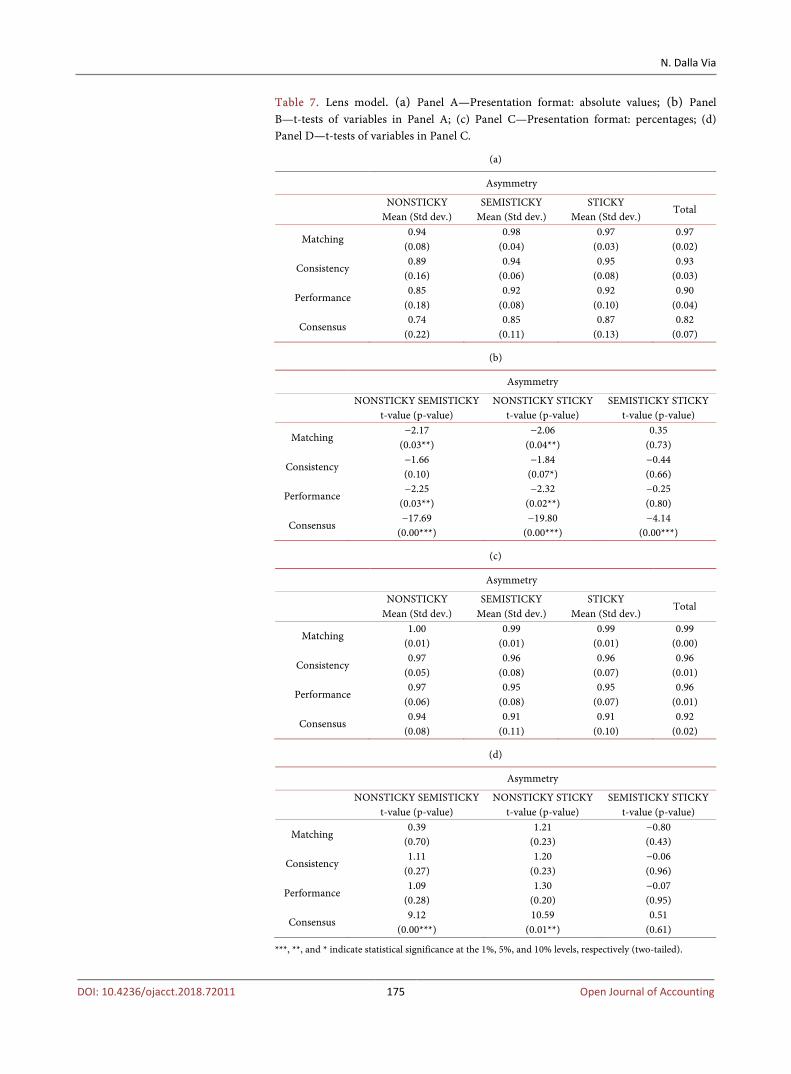
The variables of the lens model are computed and examined in Table 7. When the data are presented as absolute values, the value of matching is significantly higher in the semisticky case (0.98, p = 0.03) and in the sticky case (0.97, p = 0.04) than the nonsticky condition (0.94). However, the values of consistency are significantly different only between the two extreme cases, namely sticky and nonsticky. The performance indicator, obtained multiplying matching and con-sistency, is significantly different when comparing nonsticky and sticky condi-tions (0.85 vs. 0.92, p = 0.02) and nonsticky and semisticky conditions (0.85 vs. 0.92, p = 0.03). The last variable, called consensus, compares the judgment errors across participants. In the sticky condition the variable has the highest value (0.87), followed by the semisticky condition (0.85), and finally by the nonsticky condition (0.74). All the differences are significantly different (p < 0.01). Overall, the results of Panel A and B of Table 7 confirms the previous findings about judgment accuracy. The sticky behavior is more easily replicated than the sym-metric condition.

Panel C and D of the same table exhibit the same variables computed in the percentages presentation format. Also in this case, coherently with the previous findings, I do not find a significant difference of accuracy across degrees of asymmetry. The value of matching is on average very high (0.99) as well as the performance indicator (0.96). Significant differences are registered only by the values of consensus with an average of 0.92. The comparison between presenta-tion formats confirms the higher accuracy of percentages on absolute values and the support provided to hypothesis 2. Moreover, as stated before, the largest im-provement of matching and performance is registered when percentages, com-pared to absolute values, are introduced in the nonsticky condition.

The lens model considers the cues as a set and it correlates the overall predic-tions made by the individual with the theoretical predictions provided by the environmental model. However, the lack of focus on the specific weights as-signed to the cues does not allow the understanding of where the errors occur. Table 8 compares the coefficients in the individual policy-capturing models with the corresponding coefficients in the environmental model.

Recall that in the model of cost behavior β0 is the intercept, β1 captures the in-crease of revenues, and β2 is the coefficient associated to the dummy valorized with 1 when revenues decrease. Compared to percentages, the error in the non-sticky condition when data are presented as absolute values is significantly high-er in all the coefficients. Although in the semisticky and sticky conditions the largest deviations from the coefficients of the environmental models are com-puted in the absolute values condition, there is a tendency to overstate the values of β1 when absolute values are provided and to understate the same coefficient in the case of percentages. The accuracy of β2 is higher with percentages and in the absolute values condition it emphasizes the level of cost stickiness both in the semisticky and sticky degree of asymmetry.

A graphical comparison between individual models and environmental mod-els is provided in Figure 2. The graphs are plotted using the average coefficients

N. Dalla Via

DOI: 10.4236/ojacct.2018.72011 175 Open Journal of Accounting

Table 7. Lens model. (a) Panel A—Presentation format: absolute values; (b) Panel B—t-tests of variables in Panel A; (c) Panel C—Presentation format: percentages; (d) Panel D—t-tests of variables in Panel C.

(a)

Asymmetry

NONSTICKY

Mean (Std dev.) SEMISTICKY

Mean (Std dev.) STICKY

Mean (Std dev.) Total

Matching 0.94

(0.08) 0.98

(0.04) 0.97

(0.03) 0.97

(0.02)

Consistency 0.89

(0.16) 0.94

(0.06) 0.95

(0.08) 0.93

(0.03)

Performance 0.85

(0.18) 0.92

(0.08) 0.92

(0.10) 0.90

(0.04)

Consensus 0.74

(0.22) 0.85

(0.11) 0.87

(0.13) 0.82

(0.07)

(b)

Asymmetry

NONSTICKY SEMISTICKY

t-value (p-value) NONSTICKY STICKY

t-value (p-value) SEMISTICKY STICKY

t-value (p-value)

Matching −2.17

(0.03**) −2.06

(0.04**) 0.35

(0.73)

Consistency −1.66 (0.10)

−1.84 (0.07*)

−0.44 (0.66)

Performance −2.25

(0.03**) −2.32

(0.02**) −0.25 (0.80)

Consensus −17.69

(0.00***) −19.80

(0.00***) −4.14

(0.00***)

(c)

Asymmetry

NONSTICKY

Mean (Std dev.) SEMISTICKY

Mean (Std dev.) STICKY

Mean (Std dev.) Total

Matching 1.00

(0.01) 0.99

(0.01) 0.99

(0.01) 0.99

(0.00)

Consistency 0.97

(0.05) 0.96

(0.08) 0.96

(0.07) 0.96

(0.01)

Performance 0.97

(0.06) 0.95

(0.08) 0.95

(0.07) 0.96

(0.01)

Consensus 0.94

(0.08) 0.91

(0.11) 0.91

(0.10) 0.92

(0.02)

(d)

Asymmetry

NONSTICKY SEMISTICKY

t-value (p-value) NONSTICKY STICKY

t-value (p-value) SEMISTICKY STICKY

t-value (p-value)

Matching 0.39

(0.70) 1.21

(0.23) −0.80 (0.43)

Consistency 1.11

(0.27) 1.20

(0.23) −0.06 (0.96)

Performance 1.09

(0.28) 1.30

(0.20) −0.07 (0.95)

Consensus 9.12

(0.00***) 10.59

(0.01**) 0.51

(0.61)

***, **, and * indicate statistical significance at the 1%, 5%, and 10% levels, respectively (two-tailed).

N. Dalla Via

DOI: 10.4236/ojacct.2018.72011 176 Open Journal of Accounting

Figure 2. Policy-capturing models and environmental model across degrees of asymme-try and presentation formats. of the participants’ mental models and are compared with the theoretical model that the subjects should have learned observing the learning dataset. In order to draw the graphs, the data of the judgment dataset are applied to the models. The graphical comparison confirms visually the statistical findings.

5. Discussion and Conclusions

The literature on cost stickiness rarely considered in the analyses the individual level as possible source of determinants. However, the individual decision mak-ing affects the prediction of costs and the adjustments choices. For this reason,

N. Dalla Via

DOI: 10.4236/ojacct.2018.72011 177 Open Journal of Accounting

Table 8. Comparison of coefficients between individuals’ policy-capturing models and environmental model.

Presentation format

Absolute values Mean (Std dev.)

Percentages Mean (Std dev.)

t−value (p−value)

NONSTICKY

β0p − β0e −0.08 (0.16)

0.00 (0.03)

−3.00 (0.00***)

β1p − β1e 0.55

(1.42) −0.04 (0.28)

2.50 (0.02**)

β2p − β2e −0.87 (1.68)

0.03 (0.35)

−3.21 (0.00***)

SEMISTICKY

β0p − β0e −0.05 (0.13)

0.01 (0.03)

−2.76 (0.01***)

β1p − β1e 0.27

(0.87) −0.10 (0.23)

2.56 (0.01**)

β2p − β2e −0.28 (1.05)

0.17 (0.32)

−2.50 (0.2**)

STICKY

β0p − β0e −0.07 (0.16)

0.00 (0.03)

−2.58 (0.01**)

β1p − β1e 0.27

(0.88) −0.08 (0.19)

2.41 (0.02**)

β2p − β2e −0.20 (1.22)

0.14 (0.34)

−1.69 (0.10*)

***, **, and * indicate statistical significance at the 1%, 5%, and 10% levels, respectively (two-tailed); β0p − β0e is the difference between the coefficients of the individual policy-capturing models and the correspond-ing coefficient in the environmental model (and similarly for β1p − β1e and β2p − β2e). Coefficients in the en-vironmental models: NONSTICKY: β0 = −0.00; β1 = 0.89; β2= −0.04 SEMISTICKY: β0 = −0.00; β1 = 0.90; β2 = −0.28 STICKY: β0 = −0.01; β1 = 0.91; β2 = −0.57.

the behavioral features of the subjects and their relationships with the cost deci-sions have to be investigated. The use of subjectivity introduces cognitive biases that influence the accuracy of the decision outcomes. My experiment confirms that the presentation format of the information influences decision making as proved by many studies in the literature, but suggests also that the ability to pre-dict the trend of costs is different depending on the degree of asymmetry. More in detail, I prove that cost predictions are more accurate when data are expressed in percentages rather than absolute values. The provision of percentages, com-pared to absolute values, is more beneficial when the cost behavior is symmetric rather than sticky. Moreover, when data are presented as absolute values, the subjects mentally adopt a sticky model of cost prediction independently on the learning dataset. The tendency to inflate the increases of costs and to reduce the magnitude of the decreases in any condition is an important behavioral feature and confirms the contribution of my study to the literature on cost stickiness.

The findings of this study have important managerial implications. Overall, the results suggest that managers are influenced by cognitive biases when re-quired to prepare cost forecasts and to make cost adjustments decisions. In par-

N. Dalla Via

DOI: 10.4236/ojacct.2018.72011 178 Open Journal of Accounting

ticular, managers have a tendency to predict increases and decreases of costs as asymmetrical changes under all conditions and to apply mentally a sticky model of cost prediction. Thus, the cost stickiness behavior examined by previous lite-rature is not always the result of a deliberate managerial choice. Companies should encourage managers to prepare reports by using simple presentation formats, such as with percentages, in order to increase decision accuracy and to minimize the tendency to treat costs differently (i.e. asymmetrically) when rev-enues and production volumes increase or decrease.

The adoption of an experimental methodology is subject to limitations in the generalization of the findings. In addition, a certain level of mathematical ability, such as working with percentages and proportions, is required for my task. In order to isolate the cognitive biases, I attempted to reduce the possible con-founding effect of the different mathematical preparation of the individuals con-trolling for this particular skill. Another limitation is associated with the use of a within-subjects manipulation. To reduce the potential issues for each participant I randomized the order of the experimental conditions.

Future research should address further the issue of individual decision making focusing on how individuals mentally model the information presented in the reports and on how they draw their choices. The increasing need of timely deci-sions does not guarantee the support of complete and detailed reports, inducing the use of subjective analysis. However, the biases associated to subjectivity lead to distorted and inaccurate decisions. A deeper knowledge of these issues would help to prevent and control their emergence.

References [1] Anderson, M.C., Banker, R.D. and Janakiraman, S.N. (2003) Are Selling, General,

and Administrative Costs “Sticky”? Journal of Accounting Research, 41, 47-63. https://doi.org/10.1111/1475-679X.00095

[2] Banker, R.D., Potter, G. and Srinavasan, D. (2000) An Empirical Investigation of an Incentive Plan That Includes Nonfinancial Performance Measures. The Accounting Review, 75, 65-92. https://doi.org/10.2308/accr.2000.75.1.65

[3] Ittner, C., Larcker, D. and Meyer, M. (2003) Subjectivity and the Weighting of Per-formance Measures: Evidence from a Balanced Scorecard. The Accounting Review, 78, 725-758. https://doi.org/10.2308/accr.2003.78.3.725

[4] Tversky, A. and Kahneman, D. (1981) The Framing of Decisions and the Psycholo-gy of Choice. Science, 211, 453-458. https://doi.org/10.1126/science.7455683

[5] Harvey, N. and Bolger, F. (1996) Graphs versus Tables: Effects of Data Presentation Format on Judgemental Forecasting. International Journal of Forecasting, 12, 119-137. https://doi.org/10.1016/0169-2070(95)00634-6

[6] Lipe, M.G. and Salterio, S. (2002) A Note on the Judgmental Effects of the Balanced Scorecard’s Information Organization. Accounting, Organizations and Society, 27, 531-540. https://doi.org/10.1016/S0361-3682(01)00059-9

[7] Cardinaels, E. and Van Veen-Dirks, P.M.G. (2010) Financial versus Non-Financial Information: The Impact of Information Organization and Presentation in a Ba-lanced Scorecard. Accounting, Organizations and Society, 35, 565-578. https://doi.org/10.1016/j.aos.2010.05.003

N. Dalla Via

DOI: 10.4236/ojacct.2018.72011 179 Open Journal of Accounting

[8] Banker, R.D., Ciftci, M. and Mashruwala, R. (2014) The Moderating Effect of Prior Sales Changes on Asymmetric Cost Behavior. Journal of Management Accounting Research, 26, 221-242. https://doi.org/10.2308/jmar-50726

[9] Luft, J.L. and Shields, M.D. (2001) Why Does Fixation Persist? Experimental Evi-dence on the Judgment Performance Effects of Expensing Intangibles. The Ac-counting Review, 76, 561-587. https://doi.org/10.2308/accr.2001.76.4.561

[10] Farrell, A.M., Luft, J. and Shields, M.D. (2007) Accuracy in Judging the Nonlinear Effects of Cost and Profit Drivers. Contemporary Accounting Research, 24, 1139-1169. https://doi.org/10.1506/car.24.4.4

[11] Anderson, S.W. and Lanen, W.N. (2009) Understanding Cost Management: What Can We Learn from the Evidence on “Sticky Costs”? Working Paper, University of Michigan, Ann Arbor.

[12] Balakrishnan, R., Labro, E. and Soderstrom, N.S. (2014) Cost Structure and Sticky Costs. Journal of Management Accounting Research, 26, 91-116. https://doi.org/10.2308/jmar-50831

[13] Banker, R.D., Byzalov, D. and Plehn-Dujowich, J.M. (2011) Sticky Cost Behavior: Theory and Evidence. Working Paper, Temple University, Philadelphia.

[14] Banker, R.D. and Chen, L. (2006) Labor Market Characteristics and Cross-Country Differences in Cost Stickiness. Working Paper, Temple University, Philadelphia.

[15] Sheets, C.A. and Miller, M.J. (1974) The Effect of Cue-Criterion Function Form on Multiple-Cue Probability Learning. The American Journal of Psychology, 87, 629-641. https://doi.org/10.2307/1421971

[16] Brehmer, B., Kuylenstierna, J. and Liljergren, J. (1974) Effects of Function Form and Cue Validity on the Subjects’ Hypotheses in Probabilistic Inference Tasks. Organi-zational Behavior and Human Performance, 11, 338-354. https://doi.org/10.1016/0030-5073(74)90024-5

[17] Guiler, W.S. (1946) Difficulties Encountered in Percentage by College Freshmen. Journal of Educational Research, 40, 81-95. https://doi.org/10.1080/00220671.1946.10881493

[18] Parker, M. and Leinhardt, G. (1995) Percent: A Privileged Proportion. Review of Educational Research, 65, 421-481. https://doi.org/10.3102/00346543065004421

[19] Chatterjee, S., Heath, T.B., Milberg, S.J. and France, K.R. (2000) The Differential Processing of Price in Gains and Losses: The Effects of Frame and Need for Cogni-tion. Journal of Behavioral Decision Making, 13, 61-75. https://doi.org/10.1002/(SICI)1099-0771(200001/03)13:1<61::AID-BDM343>3.0.CO;2-J

[20] Chen, H.A. and Rao, A.R. (2007) When Two plus Two Is Not Equal to Four: Errors in Processing Multiple Percentage Changes. Journal of Consumer Research, 34, 327-340. https://doi.org/10.1086/518531

[21] Venezky, R.L. and Bregar, W.S. (1988) Different Levels of Ability in Solving Ma-thematical Word Problems. Journal of Mathematical Behavior, 7, 111-134.

[22] Fuson, K.C. and Abrahamson, D. (2005) Understanding Ratio and Proportion as an Example of the Apprehending Zone and Conceptual-Phase Problem-Solving Mod-els. In: Campbell, J., Ed., Handbook of Mathematical Cognition. New York, Psy-chology Press, 213-234.

[23] Nys, J. and Content, A. (2010) Complex Mental Arithmetic: The Contribution of the Number Sense. Canadian Journal of Experimental Psychology, 64, 215-220. https://doi.org/10.1037/a0020767

N. Dalla Via

DOI: 10.4236/ojacct.2018.72011 180 Open Journal of Accounting

[24] Lusardi, A. (2008) Financial Literacy: An Essential Tool for Informed Consumer Choice? Working Paper, Dartmouth College, Hanover.

[25] Reyna, V.F., Nelson, W., Han, P. and Dieckmann, N.F. (2009) How Numeracy In-fluences Risk Comprehension and Medical Decision Making. Psychological Bulle-tin, 135, 943-973. https://doi.org/10.1037/a0017327

[26] Stanovich, K.E. and West, R.F. (2000) Individual Differences in Reasoning: Implica-tions for the Rationality Debate. Behavioral and Brain Sciences, 23, 645-726. https://doi.org/10.1017/S0140525X00003435

[27] Evans, J.S.B.T. (2003) In Two Minds: Dual-Process Accounts of Reasoning. Trends in Cognitive Sciences, 7, 454-459. https://doi.org/10.1016/j.tics.2003.08.012

[28] Brehmer, B. (1971) Subjects’ Ability to Use Functional Rules. Psychonomic Science, 24, 259-260. https://doi.org/10.3758/BF03328999

[29] Slovic, P. (1974) Hypothesis Testing in the Learning of Positive and Negative Linear Functions. Organizational Behavior and Human Performance, 11, 368-376. https://doi.org/10.1016/0030-5073(74)90026-9

[30] Fischbacher, U. (2007) z-Tree: Zurich Toolbox for Ready-Made Economic Experi-ments. Experimental Economics, 10, 171-178. https://doi.org/10.1007/s10683-006-9159-4

[31] Schwartz, L.M.,Woloshin, S., Black, W.C. andWelch, H.G. (1997) The Role of Nu-meracy in Understanding the Benefit of Screening Mammography. Annals of In-ternal Medicine, 127, 966-972. https://doi.org/10.7326/0003-4819-127-11-199712010-00003

[32] Lipkus, I.M., Samsa, G. and Rimer, B.K. (2001) General Performance on a Nume-racy Scale among Highly Educated Samples. Medical Decision Making, 21, 37-44. https://doi.org/10.1177/0272989X0102100105

[33] Allinson, C.W. and Hayes, J. (1996) The Cognitive Style Index: A Measure of Intui-tion-Analysis for Organizational Research. Journal of Management Studies, 33, 119-135. https://doi.org/10.1111/j.1467-6486.1996.tb00801.x

[34] Sadler-Smith, E., Spicer, D.P. and Tsang, F. (2000) Validity of the Cognitive Style Index: Replication and Extension. British Journal of Management, 11, 175-181. https://doi.org/10.1111/1467-8551.t01-1-00159

[35] Frederick, S. (2005) Cognitive Reflection and Decision Making. Journal of Econom-ic Perspectives, 19, 25-42. https://doi.org/10.1257/089533005775196732

[36] Brunswik, E. (1952) The Conceptual Framework of Psychology. The University of Chicago Press, Chicago.

[37] Bonner, S.E., Walther, B.R. and Young, S.M. (2003) Sophistication-Related Differ-ences in Investors’ Models of the Relative Accuracy of Analysts’ Forecast Revisions. The Accounting Review, 78, 679-706. https://doi.org/10.2308/accr.2003.78.3.679

[38] Castellan, N.J. (1992) Relations between Linear Models: Implications for the Lens Model. Organizational Behavior and Human Decision Processes, 51, 364-381. https://doi.org/10.1016/0749-5978(92)90018-3

[39] Karelaia, N. and Hogarth, R.M. (2008) Determinants of Linear Judgment: A Me-ta-Analysis of Lens Model Studies. Psychological Bulletin, 134, 404-426. https://doi.org/10.1037/0033-2909.134.3.404