the proximal primal-dual approach for nonconvex linearly constrained...
TRANSCRIPT

The Proximal Primal-Dual Approach for NonconvexLinearly Constrained Problems
Presenter: Mingyi Hong
Joint work with Davood Hajinezhad
University of MinnesotaECE Department
DIMACS Workshop on Distributed Opt., Information Process., and LearningAugust, 2017
Mingyi Hong (University of Minnesota) 0 / 56
Agenda
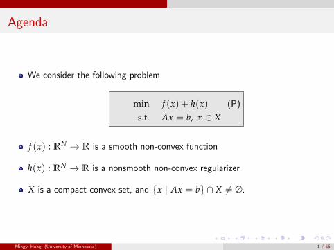
We consider the following problem
min f (x) + h(x) (P)
s.t. Ax = b, x ∈ X
f (x) : RN → R is a smooth non-convex function
h(x) : RN → R is a nonsmooth non-convex regularizer
X is a compact convex set, and {x | Ax = b} ∩ X 6= ∅.
Mingyi Hong (University of Minnesota) 1 / 56
The Plan
1 Design an efficient decomposition scheme decoupling the variables
2 Analyze convergence/rate of convergence
3 Discuss convergence to first/second-order stationary solutions
4 Explore different variants of the algorithms; obtain useful insights
5 Evaluate practical performance
Mingyi Hong (University of Minnesota) 2 / 56
App 1: Distributed optimization
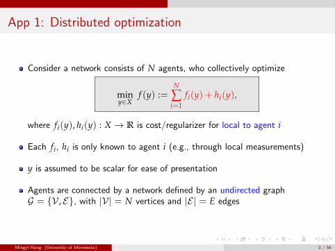
Consider a network consists of N agents, who collectively optimize
miny∈X
f (y) :=N
∑i=1
fi(y) + hi(y),
where fi(y), hi(y) : X → R is cost/regularizer for local to agent i
Each fi, hi is only known to agent i (e.g., through local measurements)
y is assumed to be scalar for ease of presentation
Agents are connected by a network defined by an undirected graphG = {V , E}, with |V| = N vertices and |E | = E edges
Mingyi Hong (University of Minnesota) 3 / 56
App 1: Distributed optimization
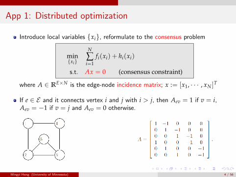
Introduce local variables {xi}, reformulate to the consensus problem
min{xi}
N
∑i=1
fi(xi) + hi(xi)
s.t. Ax = 0 (consensus constraint)
where A ∈ RE×N is the edge-node incidence matrix; x := [x1, · · · , xN ]T
If e ∈ E and it connects vertex i and j with i > j, then Aev = 1 if v = i,Aev = −1 if v = j and Aev = 0 otherwise.
Mingyi Hong (University of Minnesota) 4 / 56
App 2: Partial consensus
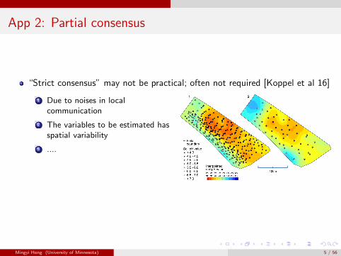
“Strict consensus” may not be practical; often not required [Koppel et al 16]
1 Due to noises in localcommunication
2 The variables to be estimated hasspatial variability
3 ....
Mingyi Hong (University of Minnesota) 5 / 56

App 2: Partial consensus
Relax the consensus requirement
mini
N
∑i=1
fi(xi) + hi(xi)
s.t. ‖xi − xj‖2 ≤ bij, ∀(i, j) ∈ E.
Introduce “link variable” {zij = xi − xj}; Equivalent reformulation
mini
N
∑i=1
fi(xi) + hi(xi)
s.t. Ax− z = 0, z ∈ Z
Mingyi Hong (University of Minnesota) 6 / 56
App 2: Partial consensus
The local cost functions can be non-convex in a number of situations
1 The use of non-convex regularizers, e.g., SCAD/MCP [Fan-Li 01, Zhang 10]
2 Non-convex quadratic functions, e.g., high-dimensional regression with missingdata [Loh-Wainwright 12], sparse PCA
3 Sigmoid loss function (approximating 0-1 loss) [Shalev-Shwartz et al 11]
4 Loss function for training neural nets [Allen-Zhu-Hazan 16]
Mingyi Hong (University of Minnesota) 7 / 56
App 3: Non-convex subspace estimation
Let Σ ∈ Rp×p be an unknown covariance matrix, with eigen-decomposition
Σ =p
∑i=1
λiuiuTi
where λ1 ≥ · · · ≥ λp are eigenvalues; u1, · · · , up are eigenvectors
The k-dimensional principal subspace of Σ
Π∗ =k
∑i=1
λiuiuTi = UUT
Principal subspace estimation. Given i.i.d samples {x1, · · · , xn}, estimateΠ∗, based on sample covariance matrix Σ
Mingyi Hong (University of Minnesota) 8 / 56
App 3: Non-convex subspace estimation
Problem formulation [Gu et al 14]
Π = arg minΠ
− 〈Σ, Π〉+ Pα(Π)
s.t. 0 � Π � I, Tr(Π) = k. (Fantope set)
where Pα(Π) is a non-convex regularizer (such as MCP/SCAD)
Estimation result. [Gu et al 14] Under certain condition on α, everyfirst-order stationary solution is “good”, with high probability:
‖Π−Π∗‖F ≤ s1
√sn+ s2
√log(p)
n
s = |supp(diag(Π∗))| is the subspace sparsity [Vu et al 13]
Mingyi Hong (University of Minnesota) 9 / 56

App 3: Non-convex subspace estimation
Question. How to find first-order stationary solution?
Need to deal with both the Fantope and non-convex regularizer Pα(Π)
A heuristic approach proposed in [Gu et al 14]
1 Introduce linear constraint X = Π
2 Impose non-convex regularizer on X, Fantope constraint on Π
Π = arg minΠ
− 〈Σ, Π〉+ Pα(X)
s.t. 0 � Π � I, Tr(Π) = k. (Fantope set)
Π− X = 0
3 Same formulation as (P), only heuristic algorithm without any guarantee
Mingyi Hong (University of Minnesota) 10 / 56

The literature
Mingyi Hong (University of Minnesota) 10 / 56

Literature
The Augmented Lagrangian (AL) methods [Hestenes 69, Powell 69], is aclassical algorithm for solving nonlinear non-convex constrained problems
Many existing packages (e.g., LANCELOT)
Recent developments [Curtis et al 16] [Friedlander 05], and many more
Convex problem + linear constraints, [Lan-Monterio 15] [Liu et al 16]analyzed the iteration complexity for the AL method
Requires double-loop
In the non-convex setting difficult to handle non-smooth regularizers
Difficult to be implemented in a distributed manner
Mingyi Hong (University of Minnesota) 11 / 56
Literature
Recent works consider AL-type methods for linearly constrained problems
Nonconvex problem + linear constraints, [Artina-Fornasier-Solombrino 13]
1 Approximate the Augmented Lagrangian using proximal point (make it convex)
2 Solve the linearly constrained convex approximation with increasing accuracy
AL based methods for smooth non-convex objective + linearly couplingconstraints [Houska-Frasch-Diehl 16]
1 AL based Alternating Direction Inexact Newton (ALADIN)
2 Combines SQP and AL, global line search, Hessian computation, etc.
Still requires double-loop
No global rate analysis
Mingyi Hong (University of Minnesota) 12 / 56
Literature
Dual decomposition [Bertsekas 99]
1 Gradient/subgradient applied to the dual
2 Convex separable objective + convex coupling constraints
3 Lots of application, e.g., in wireless communications [Palomar-Chiang 06]
Arrow-Hurwicz-Uzawa primal-dual algorithm [Arrow-Hurwicz-Uzawa 58]
1 Applied to study saddle point problems [Gol’shtein 74][Nedic-Ozdaglar 07]
2 Primal-dual hybrid gradient [Zhu-Chan 08]
3 ...
Do not to work for non-convex problem (difficult to use the dual structure)
Mingyi Hong (University of Minnesota) 13 / 56
Literature
ADMM is popular in solving linearly constrained problems
Some theoretical results for applying ADMM for non-convex problems
1 [Hong-Luo-Razaviyayn 14]: non-convex consensus and sharing
2 [Li-Pong 14], [Wang-Yin-Zeng 15], [Melo-Monterio 17] with more relaxedconditions, or faster rates
3 [Pang-Tao 17] for non-convex DC program with sharp stationary solutions
Block-wise structure, but requires a special block
Does not apply to problem (P)
Mingyi Hong (University of Minnesota) 14 / 56
The plan of the talk
First consider the simpler problem (unconstrained, smooth)
minx∈RN
f (x), s.t. Ax = b (Q)
Algorithm, analysis and discussion
First-/second order stationarity
Then generalize
Applications and numerical results
Mingyi Hong (University of Minnesota) 15 / 56

The proposed algorithms
Mingyi Hong (University of Minnesota) 15 / 56

The proposed algorithm
We draw elements form AL and Uzawa methods
The augmented Lagrangian for problem (P) is given by
Lβ(x, µ) = f (x) + 〈µ, Ax− b〉+ β
2‖Ax− b‖2
where µ ∈ RM dual variable; β > 0 penalty parameter
One primal gradient-type step + one dual gradient-type step
Mingyi Hong (University of Minnesota) 16 / 56
The proposed algorithm
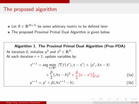
Let B ∈ RM×N be some arbitrary matrix to be defined later
The proposed Proximal Primal Dual Algorithm is given below
Algorithm 1. The Proximal Primal Dual Algorithm (Prox-PDA)
At iteration 0, initialize µ0 and x0 ∈ RN.At each iteration r + 1, update variables by:
xr+1 = arg minx∈Rn
〈∇ f (xr), x− xr〉+ 〈µr, Ax− b〉
+β
2‖Ax− b‖2 +
β
2‖x− xr‖2
BT B; (1a)
µr+1 = µr + β(Axr+1 − b). (1b)
Mingyi Hong (University of Minnesota) 17 / 56
Comments
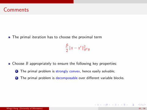
The primal iteration has to choose the proximal term
β
2‖x− xr‖2
BT B
Choose B appropriately to ensure the following key properties:
1 The primal problem is strongly convex, hence easily solvable;
2 The primal problem is decomposable over different variable blocks.
Mingyi Hong (University of Minnesota) 18 / 56
Comments
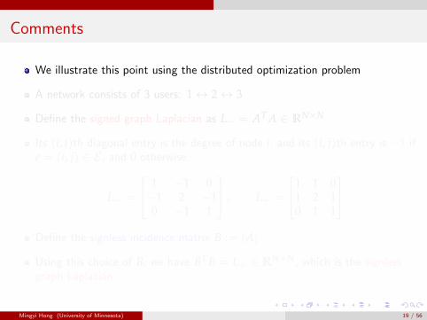
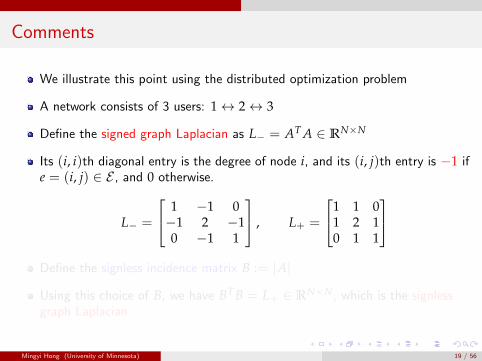
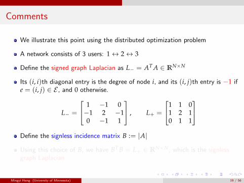
We illustrate this point using the distributed optimization problem
A network consists of 3 users: 1↔ 2↔ 3
Define the signed graph Laplacian as L− = AT A ∈ RN×N
Its (i, i)th diagonal entry is the degree of node i, and its (i, j)th entry is −1 ife = (i, j) ∈ E , and 0 otherwise.
L− =
1 −1 0−1 2 −10 −1 1
, L+ =
1 1 01 2 10 1 1
Define the signless incidence matrix B := |A|
Using this choice of B, we have BT B = L+ ∈ RN×N, which is the signlessgraph Laplacian
Mingyi Hong (University of Minnesota) 19 / 56

Comments
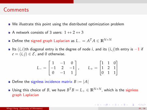
We illustrate this point using the distributed optimization problem
A network consists of 3 users: 1↔ 2↔ 3
Define the signed graph Laplacian as L− = AT A ∈ RN×N
Its (i, i)th diagonal entry is the degree of node i, and its (i, j)th entry is −1 ife = (i, j) ∈ E , and 0 otherwise.
L− =
1 −1 0−1 2 −10 −1 1
, L+ =
1 1 01 2 10 1 1
Define the signless incidence matrix B := |A|
Using this choice of B, we have BT B = L+ ∈ RN×N, which is the signlessgraph Laplacian
Mingyi Hong (University of Minnesota) 19 / 56
Comments
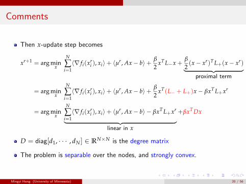
Then x-update step becomes
xr+1 = arg minx
N
∑i=1〈∇ fi(xr
i ), xi〉+ 〈µr, Ax− b〉+ β
2xT L−x +
β
2(x− xr)T L+(x− xr)︸ ︷︷ ︸
proximal term
= arg minx
N
∑i=1〈∇ fi(xr
i ), xi〉+ 〈µr, Ax− b〉+ β
2xT(L− + L+)x− βxT L+xr
= arg minx
N
∑i=1〈∇ fi(xr
i ), xi〉+ 〈µr, Ax− b〉 − βxT L+xr
︸ ︷︷ ︸linear in x
+βxT Dx
D = diag[d1, · · · , dN ] ∈ RN×N is the degree matrix
The problem is separable over the nodes, and strongly convex.
Mingyi Hong (University of Minnesota) 20 / 56

The analysis steps
Mingyi Hong (University of Minnesota) 20 / 56
Main assumptions
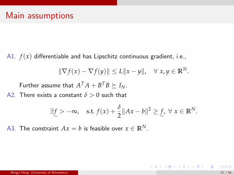
A1. f (x) differentiable and has Lipschitz continuous gradient, i.e.,
‖∇ f (x)−∇ f (y)‖ ≤ L‖x− y‖, ∀ x, y ∈ RN .
Further assume that AT A + BT B � IN .A2. There exists a constant δ > 0 such that
∃ f > −∞, s.t. f (x) +δ
2‖Ax− b‖2 ≥ f , ∀ x ∈ RN .
A3. The constraint Ax = b is feasible over x ∈ RN.
Mingyi Hong (University of Minnesota) 21 / 56

Functions satisfying the assumptions
The sigmoid function. The sigmoid function is given by
sigmoid(x) =1
1 + e−x ∈ [−1, 1].
The arctan function. arctan(x) ∈ [−1, 1] so [A2] is ok. arctan′(x) = 1x2+1 ∈ [0, 1]
so it is bounded, which implies that [A1] is true.
The tanh function. Note that we have
tanh(x) ∈ [−1, 1], tanh′(x) = 1− tanh(x)2 ∈ [0, 1].
The logit function. The logistic function is related to the tanh as
2logit(x) =2ex
ex + 1= 1 + tanh(x/2).
The quadratic function xTQx. Suppose Q is symmetric but not necessarilypositive semidefinite, and xTQx is strongly convex in the null space of AT A.
Mingyi Hong (University of Minnesota) 22 / 56

Optimality Conditions
The first and second order necessary condition for local min is given as
∇ f (x∗) + 〈µ∗, A〉 = 0, Ax∗ = b. (2a)
〈y,∇2 f (x∗)y〉 ≥ 0, ∀ y ∈ {y | Ay = 0}. (2b)
The second-order necessary condition is equivalent to the condition that∇2 f (x∗) is positive semi-definite in the null space of A
Sufficient condition for strict/strong local minimizer is given by
∇ f (x∗) + 〈µ∗, A〉 = 0, Ax∗ = b.
〈y,∇2 f (x∗)y〉 > 0, ∀ y ∈ {y | Ay = 0}.(3)
Mingyi Hong (University of Minnesota) 23 / 56
Optimality Conditions
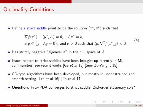
Define a strict saddle point to be the solution (x∗, µ∗) such that
∇ f (x∗) + 〈µ∗, A〉 = 0, Ax∗ = b,
∃ y ∈ {y | Ay = 0}, and σ > 0 such that 〈y,∇2 f (x∗)y〉 < 0.(4)
Has strictly negative “eigenvalue” in the null space of A.
Issues related to strict saddles have been brought up recently in MLcommunities; see recent works [Ge et al 15] [Sun-Qu-Wright 15]
GD-type algorithms have been developed, but mostly in unconstrained andsmooth setting [Lee et al 16] [Jin et al 17]
Question. Prox-PDA converges to strict saddle, 2nd-order stationary sols?
Mingyi Hong (University of Minnesota) 24 / 56
The Analysis: Step 1
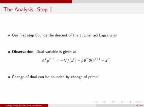
Our first step bounds the descent of the augmented Lagrangian
Observation. Dual variable is given as
ATµr+1 = −∇ f (xr)− βBT B(xr+1 − xr)
Change of dual can be bounded by change of primal
Mingyi Hong (University of Minnesota) 25 / 56
The Analysis: Step 1
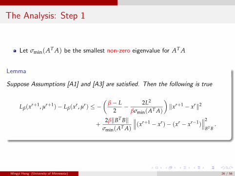
Let σmin(AT A) be the smallest non-zero eigenvalue for AT A
Lemma
Suppose Assumptions [A1] and [A3] are satisfied. Then the following is true
Lβ(xr+1, µr+1)− Lβ(xr, µr) ≤ −(
β− L2− 2L2
βσmin(AT A)
)‖xr+1 − xr‖2
+2β‖BT B‖
σmin(AT A)
∥∥∥(xr+1 − xr)− (xr − xr−1)∥∥∥2
BT B.
Mingyi Hong (University of Minnesota) 26 / 56
Comments
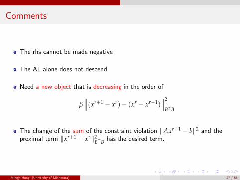
The rhs cannot be made negative
The AL alone does not descend
Need a new object that is decreasing in the order of
β∥∥∥(xr+1 − xr)− (xr − xr−1)
∥∥∥2
BT B
The change of the sum of the constraint violation ‖Axr+1 − b‖2 and theproximal term ‖xr+1 − xr‖2
BT B has the desired term.
Mingyi Hong (University of Minnesota) 27 / 56
The Analysis: Step 2
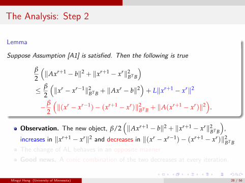
Lemma
Suppose Assumption [A1] is satisfied. Then the following is true
β
2
(‖Axr+1 − b‖2 + ‖xr+1 − xr‖2
BT B
)≤ β
2
(‖xr − xr−1‖2
BT B + ‖Axr − b‖2)+ L‖xr+1 − xr‖2
− β
2
(‖(xr − xr−1)− (xr+1 − xr)‖2
BT B + ‖A(xr+1 − xr)‖2)
.
Observation. The new object, β/2(‖Axr+1 − b‖2 + ‖xr+1 − xr‖2
BT B
),
increases in ‖xr+1 − xr‖2 and decreases in ‖(xr − xr−1)− (xr+1 − xr)‖2BT B
The change of AL behaves in an opposite manner
Good news. A conic combination of the two decreases at every iteration.
Mingyi Hong (University of Minnesota) 28 / 56

The Analysis: Step 2
Lemma
Suppose Assumption [A1] is satisfied. Then the following is true
β
2
(‖Axr+1 − b‖2 + ‖xr+1 − xr‖2
BT B
)≤ β
2
(‖xr − xr−1‖2
BT B + ‖Axr − b‖2)+ L‖xr+1 − xr‖2
− β
2
(‖(xr − xr−1)− (xr+1 − xr)‖2
BT B + ‖A(xr+1 − xr)‖2)
.
Observation. The new object, β/2(‖Axr+1 − b‖2 + ‖xr+1 − xr‖2
BT B
),
increases in ‖xr+1 − xr‖2 and decreases in ‖(xr − xr−1)− (xr+1 − xr)‖2BT B
The change of AL behaves in an opposite manner
Good news. A conic combination of the two decreases at every iteration.
Mingyi Hong (University of Minnesota) 28 / 56
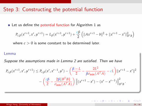
Step 3: Constructing the potential function
Let us define the potential function for Algorithm 1 as
Pc,β(xr+1, xr, µr+1) = Lβ(xr+1, µr+1) +cβ
2
(‖Axr+1 − b‖2 + ‖xr+1 − xr‖2
BT B
)where c > 0 is some constant to be determined later.
Lemma
Suppose the assumptions made in Lemma 2 are satisfied. Then we have
Pc,β(xr+1, xr, µr+1) ≤ Pc,β(xr, xr−1, µr)−(
β− L2− 2L2
βσmin(AT A)− cL
)‖xr+1 − xr‖2
−(
cβ
2− 2β‖BT B‖
σmin(AT A)
)∥∥∥(xr+1 − xr)− (xr − xr−1)∥∥∥2
BT B.
Mingyi Hong (University of Minnesota) 29 / 56
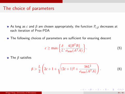
The choice of parameters
As long as c and β are chosen appropriately, the function Pc,β decreases ateach iteration of Prox-PDA
The following choices of parameters are sufficient for ensuring descent
c ≥ max{
δ
L,
4‖BT B‖σmin(AT A)
}. (5)
The β satisfies
β >L2
(2c + 1 +
√(2c + 1)2 +
16L2
σmin(AT A)
). (6)
Mingyi Hong (University of Minnesota) 30 / 56
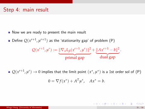
Step 4: main result
Now we are ready to present the main result
Define Q(xr+1, µr+1) as the ‘stationarity gap’ of problem (P)
Q(xr+1, µr) := ‖∇xLβ(xr+1, µr)‖2︸ ︷︷ ︸primal gap
+ ‖Axr+1 − b‖2︸ ︷︷ ︸dual gap
.
Q(xr+1, µr)→ 0 implies that the limit point (x∗, µ∗) is a 1st order sol of (P)
0 = ∇ f (x∗) + ATµ∗, Ax∗ = b.
Mingyi Hong (University of Minnesota) 31 / 56
The main result
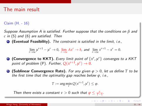
Claim (H. - 16)
Suppose Assumption A is satisfied. Further suppose that the conditions on β andc in (5) and (6) are satisfied. Then
1 (Eventual Feasibility). The constraint is satisfied in the limit, i.e.,
limr→∞
µr+1 − µr → 0, limr→∞
Axr → b, and limr→∞
xr+1 − xr = 0.
2 (Convergence to KKT). Every limit point of {xr, µr} converges to a KKTpoint of problem (P). Further, Q(xr+1, µr)→ 0.
3 (Sublinear Convergence Rate). For any given ϕ > 0, let us define T to bethe first time that the optimality gap reaches below ϕ, i.e.,
T := arg minr
Q(xr+1, µr) ≤ ϕ.
Then there exists a constant ν > 0 such that ϕ ≤ νT−1 .
Mingyi Hong (University of Minnesota) 32 / 56
Extension: Increasing the proximal parameter
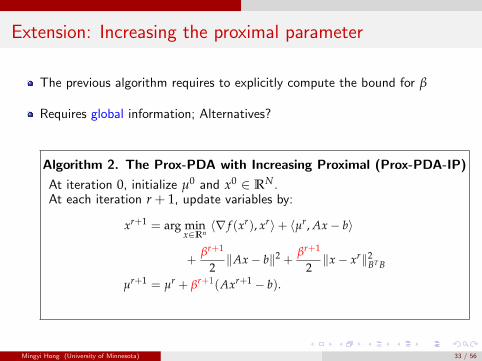
The previous algorithm requires to explicitly compute the bound for β
Requires global information; Alternatives?
Algorithm 2. The Prox-PDA with Increasing Proximal (Prox-PDA-IP)
At iteration 0, initialize µ0 and x0 ∈ RN.At each iteration r + 1, update variables by:
xr+1 = arg minx∈Rn
〈∇ f (xr), xr〉+ 〈µr, Ax− b〉
+βr+1
2‖Ax− b‖2 +
βr+1
2‖x− xr‖2
BT B
µr+1 = µr + βr+1(Axr+1 − b).
Mingyi Hong (University of Minnesota) 33 / 56
Extension: Increasing the proximal parameter
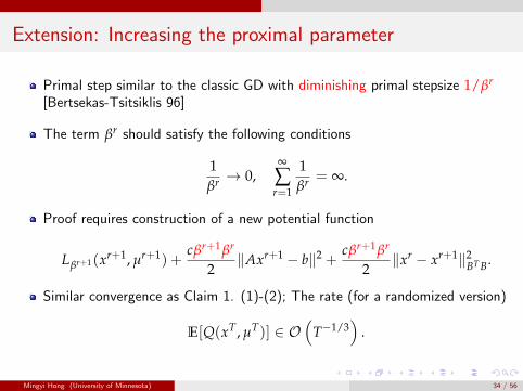
Primal step similar to the classic GD with diminishing primal stepsize 1/βr
[Bertsekas-Tsitsiklis 96]
The term βr should satisfy the following conditions
1βr → 0,
∞
∑r=1
1βr = ∞.
Proof requires construction of a new potential function
Lβr+1(xr+1, µr+1) +cβr+1βr
2‖Axr+1 − b‖2 +
cβr+1βr
2‖xr − xr+1‖2
BT B.
Similar convergence as Claim 1. (1)-(2); The rate (for a randomized version)
E[Q(xT , µT)] ∈ O(
T−1/3)
.
Mingyi Hong (University of Minnesota) 34 / 56
Second order stationary solutions?
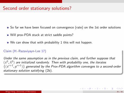
So far we have been focused on convergence (rate) on the 1st order solutions
Will prox-PDA stuck at strict saddle points?
We can show that with probability 1 this will not happen.
Claim (H.-Razaviyayn-Lee 17)
Under the same assumption as in the previous claim, and further suppose that(x0, λ0) are initialized randomly. Then with probability one, the iterates{(xr+1, µr+1)} generated by the Prox-PDA algorithm converges to a second-orderstationary solution satisfying (2b).
Mingyi Hong (University of Minnesota) 35 / 56
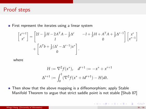
Proof steps
First represent the iterates using a linear system[xr+1
xr
]=
[2I − 1
β H − 2AT A− 1β ∆r −I + 1
β H + AT A + 1β ∆r−1
I 0
] [xr
xr−1
]
+
[ATb + 1
β (∆r − ∆r−1)x∗
0
].
where
H := ∇2 f (x∗), dr+1 := −x∗ + xr+1
∆r+1 :=∫ 1
0(∇2 f (x∗ + tdr+1)− H)dt.
Then show that the above mapping is a diffeomorphism; apply StableManifold Theorem to argue that strict saddle point is not stable [Shub 87]
Mingyi Hong (University of Minnesota) 36 / 56

Generalize to (P)?
Mingyi Hong (University of Minnesota) 36 / 56
Generalize to (P)?
Can we generalize the Prox-PDA to the following problem?
min f (x) + h(x) (P)
s.t. Ax = b, x ∈ X
With the following assumptions
B1 h(x) = g0(x) + h0(x) a non-convex regularizer; g0 is smooth non-convex,h0(x) is nonsmooth convex (such as the MCP/SCAD regularizer)
B2 X is a closed compact convex set
Mingyi Hong (University of Minnesota) 37 / 56
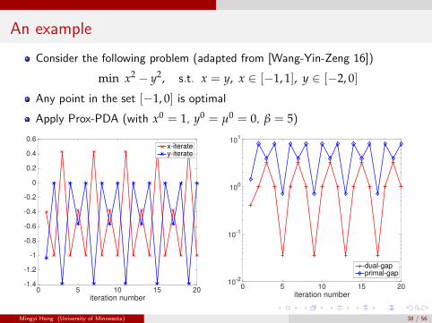
An example
Consider the following problem (adapted from [Wang-Yin-Zeng 16])
min x2 − y2, s.t. x = y, x ∈ [−1, 1], y ∈ [−2, 0]
Any point in the set [−1, 0] is optimal
Apply Prox-PDA (with x0 = 1, y0 = µ0 = 0, β = 5)
0 5 10 15 20iteration number
-1.4
-1.2
-1
-0.8
-0.6
-0.4
-0.2
0
0.2
0.4
0.6x-iteratey-iterate
0 5 10 15 20iteration number
10-2
10-1
100
101
dual-gapprimal-gap
Mingyi Hong (University of Minnesota) 38 / 56

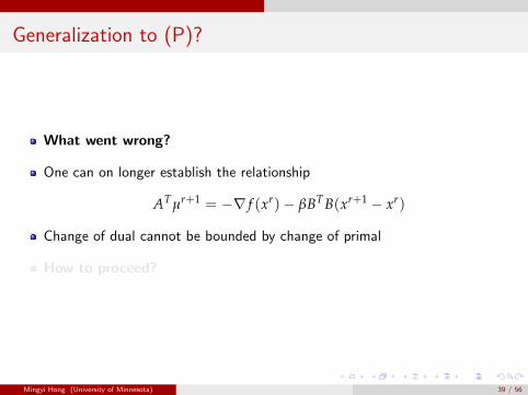
Generalization to (P)?
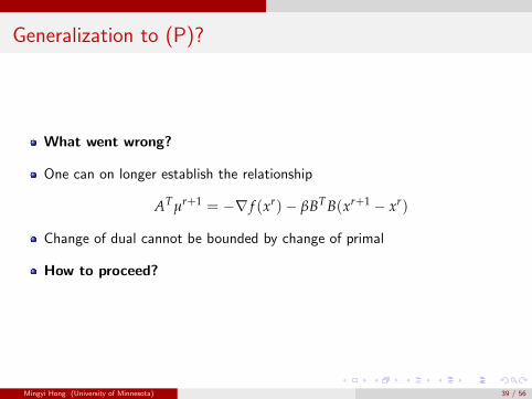
What went wrong?
One can on longer establish the relationship
ATµr+1 = −∇ f (xr)− βBT B(xr+1 − xr)
Change of dual cannot be bounded by change of primal
How to proceed?
Mingyi Hong (University of Minnesota) 39 / 56
Generalization to (P)?
What went wrong?
One can on longer establish the relationship
ATµr+1 = −∇ f (xr)− βBT B(xr+1 − xr)
Change of dual cannot be bounded by change of primal
How to proceed?
Mingyi Hong (University of Minnesota) 39 / 56
Generalization to (P)?
What went wrong?
One can on longer establish the relationship
ATµr+1 = −∇ f (xr)− βBT B(xr+1 − xr)
Change of dual cannot be bounded by change of primal
How to proceed?
Mingyi Hong (University of Minnesota) 39 / 56

Adding perturbation
The key idea is to perturb the primal-dual iteration
We perturb the dual update by
µr+1 = µr + ρr+1(
Axr+1 − b− γr+1µr)
Perturb the primal by multiplying (1− ρr+1γr+1) in front of 〈µr, Ax− b〉
Gradually reduce the size of the perturbation constant γ
Note: perturbing dual ascent- type methods has been considered for convexproblems [Koshal- Nedic-Shanbhag 11]; not perturbing primal
Mingyi Hong (University of Minnesota) 40 / 56
The Perturbed Prox-PDA
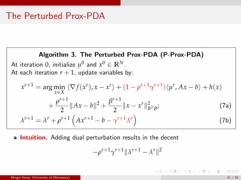
Algorithm 3. The Perturbed Prox-PDA (P-Prox-PDA)
At iteration 0, initialize µ0 and x0 ∈ RN.At each iteration r + 1, update variables by:
xr+1 = arg minx∈X〈∇ f (xr), x− xr〉+ (1− ρr+1γr+1)〈µr, Ax− b〉+ h(x)
+ρr+1
2‖Ax− b‖2 +
βr+1
2‖x− xr‖2
BT B; (7a)
λr+1 = λr + ρr+1(
Axr+1 − b− γr+1λr)
(7b)
Intuition. Adding dual perturbation results in the decent
−ρr+1γr+1‖λr+1 − λr‖2
Mingyi Hong (University of Minnesota) 41 / 56
Conditions on the sequences
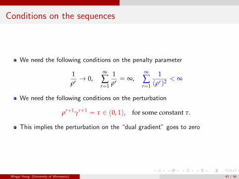
We need the following conditions on the penalty parameter
1ρr → 0,
∞
∑r=1
1ρr = ∞,
∞
∑r=1
1(ρr)2 < ∞
We need the following conditions on the perturbation
ρr+1γr+1 = τ ∈ (0, 1), for some constant τ.
This implies the perturbation on the “dual gradient” goes to zero
Mingyi Hong (University of Minnesota) 42 / 56

Outline of convergence result for P-Prox-PDA
Suppose Assumption A and B are satisfied
The conditions on {ρr, βr} and {γr} given above are satisfied; Then
limr→∞
µr+1 − µr → 0, limr→∞
Axr → b, and limr→∞
xr+1 − xr = 0
Every limit point of {xr, µr} converges to a first order stationary point of (P)[Hong.-Hajinezhad 17]
A randomized version of the algorithm converges with a rate
E[Q(xT , µT)] ∈ O(
T−1/3)
.
Mingyi Hong (University of Minnesota) 43 / 56
Remarks
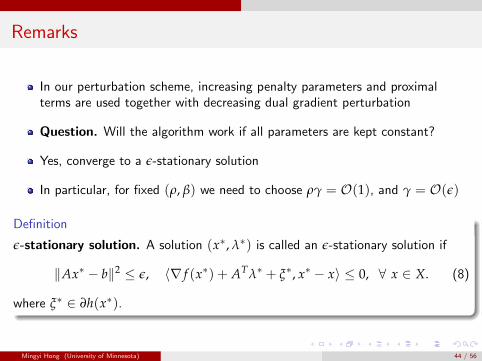
In our perturbation scheme, increasing penalty parameters and proximalterms are used together with decreasing dual gradient perturbation
Question. Will the algorithm work if all parameters are kept constant?
Yes, converge to a ε-stationary solution
In particular, for fixed (ρ, β) we need to choose ργ = O(1), and γ = O(ε)
Definition
ε-stationary solution. A solution (x∗, λ∗) is called an ε-stationary solution if
‖Ax∗ − b‖2 ≤ ε, 〈∇ f (x∗) + ATλ∗ + ξ∗, x∗ − x〉 ≤ 0, ∀ x ∈ X. (8)
where ξ∗ ∈ ∂h(x∗).
Mingyi Hong (University of Minnesota) 44 / 56

Applications
Mingyi Hong (University of Minnesota) 44 / 56

A toy example
Apply the perturbed version of Prox-PDA to the example
min x2 − y2, s.t. x = y, x ∈ [−1, 1], y ∈ [−2, 0]
With ρr = r, γr = 0.001/ρr, β = 5
0 5 10 15 20iteration number
-2
-1.5
-1
-0.5
0
0.5
1x-iteratey-iterate
0 5 10 15 20iteration number
10-10
10-8
10-6
10-4
10-2
100
102
dual-gapprimal-gap
Mingyi Hong (University of Minnesota) 45 / 56
Application to distributed non-convex optimization
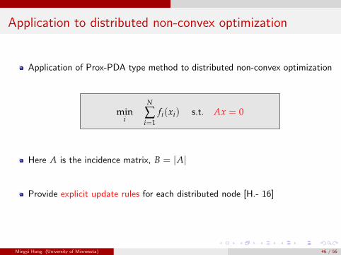
Application of Prox-PDA type method to distributed non-convex optimization
mini
N
∑i=1
fi(xi) s.t. Ax = 0
Here A is the incidence matrix, B = |A|
Provide explicit update rules for each distributed node [H.- 16]
Mingyi Hong (University of Minnesota) 46 / 56
Application to distributed non-convex optimization
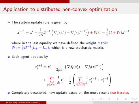
The system update rule is given by
xr+1 = xr − 12β
D−1(∇ f (xr)−∇ f (xr−1)
)+ Wxr − 1
2(I + W)xr−1
where in the last equality we have defined the weight matrixW := 1
2 D−1(L+ − L−), which is a row stochastic matrix.
Each agent updates by
xr+1i = xr
i −1
2βdi
(∇ fi(xr
i )−∇ fi(xr−1i )
)+ ∑
j∈N (i)
1di
xrj −
12
∑j∈N (i)
1di
xr−1j + xr−1
i
Completely decoupled, new update based on the most recent two iterates
Mingyi Hong (University of Minnesota) 47 / 56

Application to distributed non-convex optimization
Interestingly, such iteration has the same form as the EXTRA [Shi et al 14],developed for convex consensus problem
The same observation has also been made in [Mokhtari-Ribeiro 16] (in theconvex case)
By appealing to our analysis, the EXTRA works for the non-convexdistributed optimization problem as well (with appropriate β)
Converges (with sublinear rate) to both 1st and 2nd order stationary solutions
Different proof techniques
Other variants of Prox-PDA also can be specialized in this case
Mingyi Hong (University of Minnesota) 48 / 56
Numerical result for distributed non-convex optimization
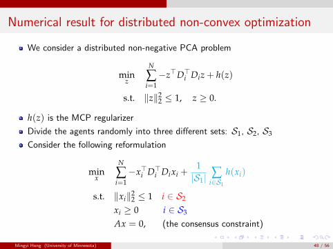
We consider a distributed non-negative PCA problem
minz
N
∑i=1−z>D>i Diz + h(z)
s.t. ‖z‖22 ≤ 1, z ≥ 0.
h(z) is the MCP regularizer
Divide the agents randomly into three different sets: S1, S2, S3
Consider the following reformulation
minx
N
∑i=1−x>i D>i Dixi +
1|S1| ∑
i∈S1
h(xi)
s.t. ‖xi‖22 ≤ 1 i ∈ S2
xi ≥ 0 i ∈ S3
Ax = 0, (the consensus constraint)
Mingyi Hong (University of Minnesota) 48 / 56
Numerical result for distributed non-convex optimization
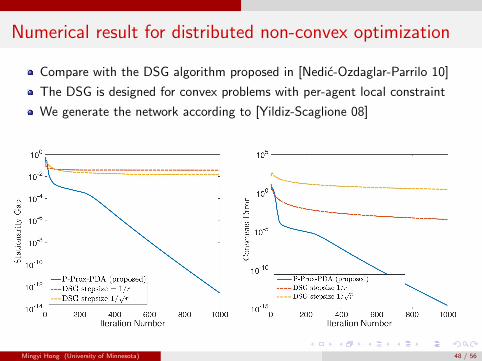
Compare with the DSG algorithm proposed in [Nedic-Ozdaglar-Parrilo 10]
The DSG is designed for convex problems with per-agent local constraint
We generate the network according to [Yildiz-Scaglione 08]
Mingyi Hong (University of Minnesota) 48 / 56
Numerical result for distributed non-convex optimization
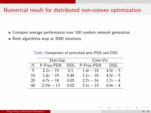
Compare average performance over 100 random network generation
Both algorithms stop at 2000 iterations
Table: Comparison of perturbed prox-PDA and DSG
Stat-Gap Cons-VioN P-Prox-PDA DSG P-Prox-PDA DSG5 2.1e− 19 0.1 1.4e− 18 4.5e− 5
10 1.4e− 19 0.48 1.1e− 18 4.5e− 520 6.7e− 18 0.05 2.7e− 16 1.7e− 440 2.19e− 13 0.02 3.1e− 15 6.9e− 4
Mingyi Hong (University of Minnesota) 48 / 56
Application to sparse subspace estimation
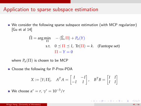
We consider the following sparse subspace estimation (with MCP regularizer)[Gu et al 14]
Π = arg minΠ
− 〈Σ, Π〉+ Pα(Y)
s.t. 0 � Π � I, Tr(Π) = k. (Fantope set)Π−Y = 0
where Pα(Π) is chosen to be MCP
Choose the following for P-Prox-PDA
X := [Y; Π], AT A =
[I −I−I I
], BT B =
[I II I
]We choose αr = r, γr = 10−3/r
Mingyi Hong (University of Minnesota) 49 / 56
Application to sparse subspace estimation
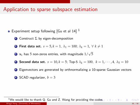
Experiment setup following [Gu et al 14] 1
1 Construct Σ by eigen-decomposition
2 First data set. s = 5, k = 1, λ1 = 100; λk = 1, ∀ k 6= 1
3 x1 has 5 non-zeros entries, with magnitude 1/√
5
4 Second data set. s = 10, k = 5; Top-5 λk = 100, k = 1, · · · , 4, λ5 = 10
5 Eigenvectors are generated by orthnormalizing a 10-sparse Gaussian vectors
6 SCAD regularizer, b = 3
1We would like to thank Q. Gu and Z. Wang for providing the codes.Mingyi Hong (University of Minnesota) 50 / 56

Application to sparse subspace estimation
We show one realization of P-Prox-PDA and the algorithm in [Gu et al 14]
Consider the scenario where n = 80, p = 128, k = 1, s = 5
0 50 100 150 200Iteration Number
10-10
10-8
10-6
10-4
10-2
100
Stationarity
Gap
P- Prox-PDA (proposed)[Gu et al 14] ρ=5[Gu et al 14] ρ=2
0 50 100 150 200Iteration Number
10-10
10-8
10-6
10-4
10-2
100
ConstraintViolation
P-Prox-PDA (proposed)[Gu et al 14] ρ=5[Gu et al 14] ρ=2
Mingyi Hong (University of Minnesota) 51 / 56
Application to sparse subspace estimation
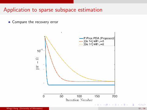
Compare the recovery error
Mingyi Hong (University of Minnesota) 52 / 56

Application to sparse subspace estimation
Compare the averaged performance of different algorithms
Generate 100 true covariance matrices Σ; for each Σ, generate 100 samples
Table: Subspace Estimation Error
‖Π−Π∗‖Parameters PPD [Gu et al 14]
n = 80, p = 128, k = 1, s = 5 0.031± 0.01 0.033± 0.01n = 150, p = 200, k = 1, s = 5 0.022± 0.07 0.025± 0.08n = 80, p = 128, k = 1, s = 10 0.047± 0.01 0.063± 0.01n = 80, p = 128, k = 5, s = 10 0.24± 0.05 0.31± 0.02n = 70, p = 128, k = 5, s = 10 0.23± 0.03 0.33± 0.03
n = 128, p = 128, k = 5, s = 10 0.17± 0.02 0.25± 0.02
Mingyi Hong (University of Minnesota) 53 / 56
Application to sparse subspace estimation
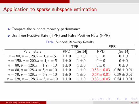
Compare the support recovery performance
Use True Positive Rate (TPR) and False Positive Rate (FPR)
Table: Support Recovery Results
TPR FPRParameters PPD [Gu 14] PPD [Gu 14]
n = 80, p = 128, k = 1, s = 5 1± 0 1± 0 0± 0 0± 0n = 150, p = 200, k = 1, s = 5 1± 0 1± 0 0± 0 0± 0n = 80, p = 128, k = 1, s = 10 1± 0 1± 0 0± 0 0± 0n = 80, p = 128, k = 5, s = 10 1± 0 1± 0 0.53± 0.03 0.56± 0.04n = 70, p = 128, k = 5, s = 10 1± 0 1± 0 0.57± 0.01 0.59± 0.02
n = 128, p = 128, k = 5, s = 10 1± 0 1± 0 0.53± 0.05 0.54± 0.01
Mingyi Hong (University of Minnesota) 54 / 56
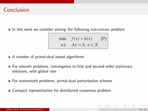
Conclusion
In this work we consider solving the following non-convex problem
min f (x) + h(x) (P)
s.t. Ax = b, x ∈ X
A number of primal-dual based algorithms
For smooth problems, convergence to first and second order stationarysolutions, with global rate
For nonsmooth problems, primal-dual perturbation scheme
Compact representation for distributed consensus problem
Mingyi Hong (University of Minnesota) 55 / 56

Future Works
How about 2nd-order stationarity for non-smooth, constrained problems?
Preliminary results reported in [Chang-H.-Pang 17], use (single-sided) secondorder directional derivative to characterize
The resulting condition is much more complicated than that for theunconstrained linearly constrained case; checking those conditions could beNP-hard; Efficient algorithms?
Stochasticity? What if objective/gradient is only known through a noisyfirst/zeroth order oracle?
More applications: Mumford-Shah regularization for image processing (e.g.,inpainting) [Mollenhoff et al 14]; Topic modeling [Fu et al 16]; etc.
Mingyi Hong (University of Minnesota) 56 / 56

Thank You!
Mingyi Hong (University of Minnesota) 56 / 56
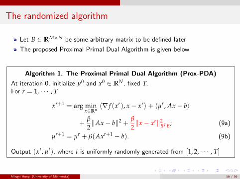
The randomized algorithm
Let B ∈ RM×N be some arbitrary matrix to be defined later
The proposed Proximal Primal Dual Algorithm is given below
Algorithm 1. The Proximal Primal Dual Algorithm (Prox-PDA)
At iteration 0, initialize µ0 and x0 ∈ RN, fixed T.For r = 1, · · · , T
xr+1 = arg minx∈Rn
〈∇ f (xr), x− xr〉+ 〈µr, Ax− b〉
+β
2‖Ax− b‖2 +
β
2‖x− xr‖2
BT B; (9a)
µr+1 = µr + β(Axr+1 − b). (9b)
Output (xt, µt), where t is uniformly randomly generated from [1, 2, · · · , T]
Mingyi Hong (University of Minnesota) 56 / 56