nonconvex robust optimization - department of industrial

Nonconvex Robust Optimization

by

Kwong Meng Teo

B.Eng., Electrical & Electronics Engineering, University ofManchester Institute of Science and Technology (1993)

M.Sc., Electrical Engineering, National University of Singapore (1999)S.M., High Performance Computing, Singapore-MIT Alliance (2000)

Submitted to the Sloan School of Managementin partial fulfillment of the requirements for the degree of

Doctor of Philosophy in Operations Research

at the

MASSACHUSETTS INSTITUTE OF TECHNOLOGY

June 2007

c© Massachusetts Institute of Technology 2007. All rights reserved.

Author . . . . . . . . . . . . . . . . . . . . . . . . . . . . . . . . . . . . . . . . . . . . . . . . . . . . . . . . . . . . . .Sloan School of Management

May 4, 2007

Certified by. . . . . . . . . . . . . . . . . . . . . . . . . . . . . . . . . . . . . . . . . . . . . . . . . . . . . . . . . .Dimitris J. Bertsimas

Boeing Professor of Operations ResearchSloan School of Management

Thesis Supervisor

Accepted by . . . . . . . . . . . . . . . . . . . . . . . . . . . . . . . . . . . . . . . . . . . . . . . . . . . . . . . . .Cynthia Barnhart

Professor, Civil and Environmental EngineeringOperations Research Center


by

Kwong Meng Teo

Submitted to the Sloan School of Managementon May 4, 2007, in partial fulfillment of the

requirements for the degree ofDoctor of Philosophy in Operations Research

Abstract

We propose a novel robust optimization technique, which is applicable to nonconvexand simulation-based problems. Robust optimization finds decisions with the bestworst-case performance under uncertainty. If constraints are present, decisions shouldalso be feasible under perturbations. In the real-world, many problems are noncon-vex and involve computer-based simulations. In these applications, the relationshipbetween decision and outcome is not defined through algebraic functions. Instead,that relationship is embedded within complex numerical models. Since current robustoptimization methods are limited to explicitly given convex problems, they cannotbe applied to many practical problems. Our proposed method, however, operates onarbitrary objective functions. Thus, it is generic and applicable to most real-worldproblems. It iteratively moves along descent directions for the robust problem, andterminates at a robust local minimum. Because the concepts of descent directionsand local minima form the building blocks of powerful optimization techniques, ourproposed framework shares the same potential, but for the richer, and more realistic,robust problem. To admit additional considerations including parameter uncertain-ties and nonconvex constraints, we generalized the basic robust local search. In eachcase, only minor modifications are required - a testimony to the generic nature of themethod, and its potential to be a component of future robust optimization techniques.We demonstrated the practicability of the robust local search technique in two real-world applications: nanophotonic design and Intensity Modulated Radiation Therapy(IMRT) for cancer treatment. In both cases, the numerical models are verified by ac-tual experiments. The method significantly improved the robustness for both designs,showcasing the relevance of robust optimization to real-world problems.

Thesis Supervisor: Dimitris J. BertsimasTitle: Boeing Professor of Operations ResearchSloan School of Management

3

Acknowledgments

I would like to thank my thesis committee members, Dimitris Bertsimas, John Tsit-

siklis and Pablo Parrilo for their valuable time, suggestions and comments.

This thesis is a culmination of five years of interesting research with Dimitris.

His taste and emphasis on general practical OR techniques has left a mark on me; I

have also benefited from his perspective, experiences and access to applications from

diverse fields. His energy and drive is certainly inspirational; his encouragement and

motivation memorable.

The approach of employing scientific-mathematical analysis to make better deci-

sions is in my blood. In my opinion, it is something everyone should do - a riskless

arbitrage. My interest in computation and modeling led to a Masters degree with

the Singapore-MIT Alliance. During which, I met Dimitris, and made a good friend

in Melvyn Sim. However, pursuing a Ph.D. has never crossed my mind until a fortu-

itous five minute conversation with Melvyn in 2001. By then, he had forged a close

working relationship with Dimitris. Their enthusiasm in research infected me; their

encouragement was instrumental to my arrival in MIT. Furthermore, their world-class

research in Robust Optimization gave me both a front row seat and a first-rate train-

ing in this exciting and highly relevant field. Thus, I would like to extend my sincere

gratefulness to both of them.

Omid Nohadani is another person who had assisted me greatly. His skills in

porting the nanophotonic numerical model from Matlab to Fortran enabled a quantum

leap in the results obtained. I am also thankful for his patience in reviewing both my

thesis and my defense presentation slides.

With reference to the nanophotonic design application, I would also like to thank

D. Healy, A. Levi, P. Seliger and the research team from the University of Southern

California for their encouragement and fruitful discussions on the subject matter.

That part of the work is partially supported by DARPA - N666001-05-1-6030. I

am also grateful to Thomas Bortfeld, David Craft and Valentina Cacchiani for their

assistance in the IMRT application.

5

The ORC has a unique environment. We are techies bunking in with the Sloanies;

the result is a cozy habitat. I enjoyed diverse discussions with friends including

Margret Bjarnadottir, Timothy Chan, Lincoln Chandler, David Czerwinski, Xuan

Vinh Doan, Shobhit Gupta, Pranava Goundan, Pavithra Harsha, Kathryn Kaminski,

Carol Meyers, Dung Tri Nguyen, Carine Simon, Christopher Siow, Raghavendran

Sivaraman, Dan Stratila, Andy Sun and Ping Xu.

I am greatly indebted to my parents and my siblings for their nurture, upbringing

and unconditional love. I am also immensely grateful to my in-laws for their emotional

support and frequent visits across the oceans. The distance between Boston and

Singapore is certainly reduced by the care, concern and love showered by them.

To my little daughter Jay: you have brought immeasurable joy and love to this

world. I want you to always be so energetic and enthusiastic about life. We will talk

about this thesis and reflect on the times in Boston one day.

Finally, I want to dedicate this thesis to my loving wife, Charlotte. Through her

unwavering dedication and support, she has played a significant supporting role in

bringing this thesis to its fruition. She has given up a comfortable job in Nokia and

an easy life in Singapore when moving to Boston. Without her securing a good job in

US, her tending to domestic matters and her constant encouragements, I would not

have made it through the program so smoothly. For behind every good thesis by a

married man, there is a great woman.

Kwong Meng Teo

[email protected]

May, 2007

6

Contents

1 Introduction 21

1.1 Motivation . . . . . . . . . . . . . . . . . . . . . . . . . . . . . . . . . 22

1.2 Literature Review . . . . . . . . . . . . . . . . . . . . . . . . . . . . . 24

1.3 Structure of the Thesis . . . . . . . . . . . . . . . . . . . . . . . . . . 25

2 Nonconvex Robust Optimization for Unconstrained Problems 27

2.1 The Robust Optimization Problem Under Implementation Errors . . 28

2.1.1 Problem Definition . . . . . . . . . . . . . . . . . . . . . . . . 28

2.1.2 A Graphical Perspective of the Robust Problem . . . . . . . . 29

2.1.3 Descent Directions . . . . . . . . . . . . . . . . . . . . . . . . 29

2.1.4 Proof of Theorem 1 . . . . . . . . . . . . . . . . . . . . . . . . 32

2.1.5 Robust Local Minima . . . . . . . . . . . . . . . . . . . . . . . 35

2.1.6 A Local Search Algorithm for the Robust Optimization Problem 38

2.1.7 Practical Implementation . . . . . . . . . . . . . . . . . . . . . 42

2.2 Local Search Algorithm when Implementation Errors are present . . . 44

2.2.1 Neighborhood Search . . . . . . . . . . . . . . . . . . . . . . . 45

2.2.2 Robust Local Move . . . . . . . . . . . . . . . . . . . . . . . . 46

2.3 Application I - A Problem with a Nonconvex Polynomial Objective

Function . . . . . . . . . . . . . . . . . . . . . . . . . . . . . . . . . . 49

2.3.1 Problem Description . . . . . . . . . . . . . . . . . . . . . . . 49

2.3.2 Computation Results . . . . . . . . . . . . . . . . . . . . . . . 50

2.4 Generalized Method for Problems with Both Implementation Errors

and Parameter Uncertainties . . . . . . . . . . . . . . . . . . . . . . . 53

7


2.4.2 Basic Idea Behind Generalization . . . . . . . . . . . . . . . . 54

2.4.3 Generalized Local Search Algorithm . . . . . . . . . . . . . . . 55

2.5 Application II - Problem with Implementation and Parameter Uncer-

tainties . . . . . . . . . . . . . . . . . . . . . . . . . . . . . . . . . . . 56



2.6 Improving the Efficiency of the Robust Local Search . . . . . . . . . . 59

2.7 Robust Optimization for Problems Without Gradient Information . . 62

2.8 Conclusions . . . . . . . . . . . . . . . . . . . . . . . . . . . . . . . . 63

3 Nonconvex Robust Optimization in Nano-Photonics 65

3.1 Model . . . . . . . . . . . . . . . . . . . . . . . . . . . . . . . . . . . 68

3.2 Robust Optimization Problem . . . . . . . . . . . . . . . . . . . . . . 71

3.2.1 Nominal Optimization Problem . . . . . . . . . . . . . . . . . 72

3.2.2 Nominal Optimization Results . . . . . . . . . . . . . . . . . . 74

3.2.3 Robust Local Search Algorithm . . . . . . . . . . . . . . . . . 75


3.3 Sensitivity Analysis . . . . . . . . . . . . . . . . . . . . . . . . . . . . 79

3.4 Conclusions . . . . . . . . . . . . . . . . . . . . . . . . . . . . . . . . 79

4 Nonconvex Robust Optimization for Problems with Constraints 81

4.1 Constrained Problem under Implementations Errors . . . . . . . . . . 83


4.1.2 Robust Local Search for Problems with Constraints . . . . . . 84

4.1.3 Enhancements when Constraints are Simple . . . . . . . . . . 89

4.1.4 Constrained Robust Local Search Algorithm . . . . . . . . . . 90

4.1.5 Practical Considerations . . . . . . . . . . . . . . . . . . . . . 93

4.2 Generalization to Include Parameter Uncertainties . . . . . . . . . . . 93


4.2.2 Generalized Constrained Robust Local Search Algorithm . . . 94

8

4.3 Application III: Problem with Polynomial Cost Function and Constraints 97



4.4 Application IV: Polynomial Problem with Simple Constraints . . . . 102



4.5 Application V: A Problem in Intensity Modulated Radiation Therapy

(IMRT) for Cancer Treatment . . . . . . . . . . . . . . . . . . . . . . 106


4.5.2 Comparison with Convex Robust Optimization Techniques . . 115

4.6 Conclusions . . . . . . . . . . . . . . . . . . . . . . . . . . . . . . . . 121

5 Conclusions 123

5.1 Areas for Future Research . . . . . . . . . . . . . . . . . . . . . . . . 124

A Robust Local Search (Matlab Implementation) 127

A.1 Introduction . . . . . . . . . . . . . . . . . . . . . . . . . . . . . . . . 127

A.2 Files Included . . . . . . . . . . . . . . . . . . . . . . . . . . . . . . . 127

A.3 Pseudocode of the Robust Local Search Algorithm . . . . . . . . . . . 129

A.4 Required changes for a new problem . . . . . . . . . . . . . . . . . . 129

9

List of Figures

2-1 A 2-D illustration of the neighborhood N = {x | ‖x− x‖2 ≤ Γ}. The shaded

circle contains all possible realizations when implementing x, when we have

errors ∆x ∈ U . The bold arrow d shows a possible descent direction pointing

away from all the worst implementation errors ∆x∗i , represented by thin

arrows. All the descent directions lie within the cone, which is of a darker

shade and demarcated by broken lines. . . . . . . . . . . . . . . . . . . . . . 30

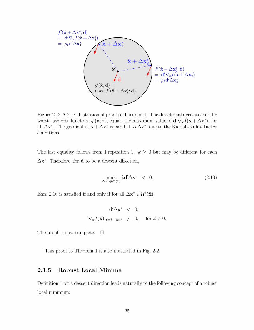
2-2 A 2-D illustration of proof to Theorem 1. The directional derivative of the

worst case cost function, g′(x;d), equals the maximum value of d′∇xf(x +

∆x∗), for all ∆x∗. The gradient at x + ∆x∗ is parallel to ∆x∗, due to the

Karush-Kuhn-Tucker conditions. . . . . . . . . . . . . . . . . . . . . . . . . 35

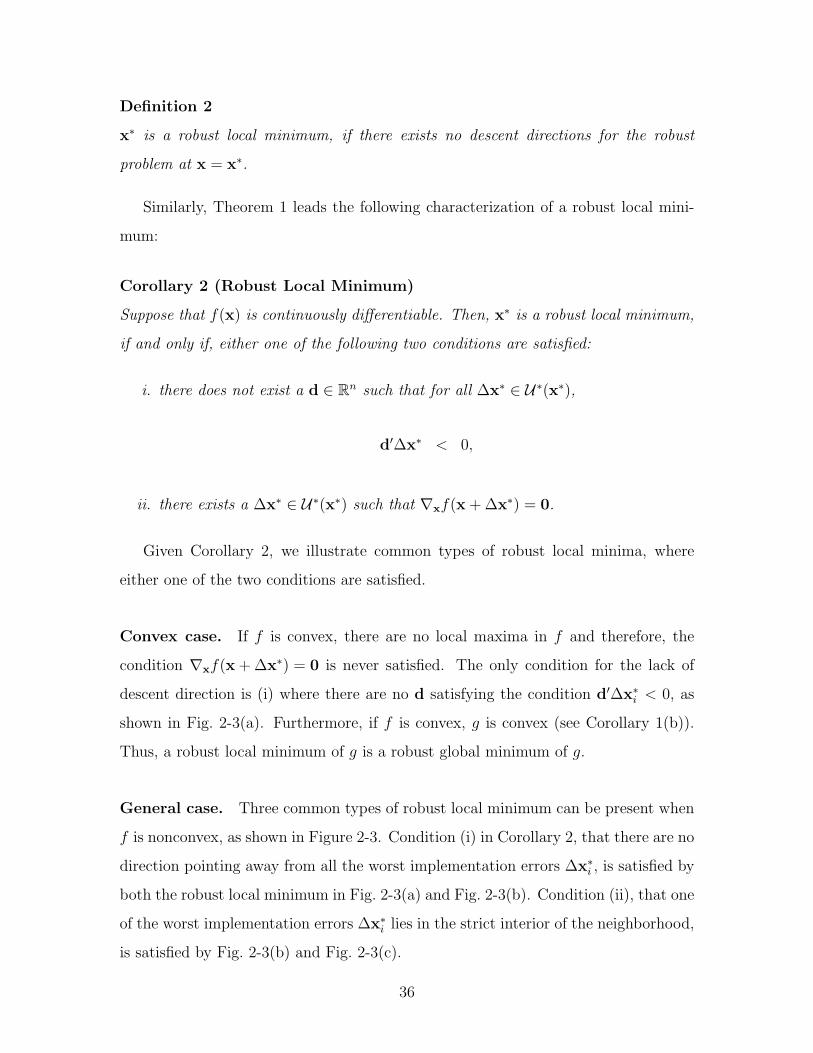
2-3 A 2-D illustration of common types of robust local minima. In (a) and

(b), there are no direction pointing away from all the worst implementation

errors ∆x∗i , which are denoted by arrows. In (b) and (c), one of the worst

implementation errors ∆x∗i lie in the strict interior of the neighborhood.

Note, for convex problems, the robust local (global) minimum is of the type

shown in (a). . . . . . . . . . . . . . . . . . . . . . . . . . . . . . . . . . . . 37

2-4 A 2-D illustration of the optimal solution of SOCP, Prob. (2.11), in the

neighborhood of x. The solid arrow indicates the optimal direction d∗ which

makes the largest possible angle θmax with all the vectors ∆x∗, ∆x∗ being

the worst case implementation errors at x. The angle θmax = cos−1 β∗ and is

at least 90o due to the constraint β ≤ −ε, ε being a small positive scalar. . . 39

2-5 −d∗ is a subgradient for g(x) because it lies within the cone spanned by ∆x∗. 42

11

2-6 The solid bold arrow indicates a direction d pointing away from all the im-

plementation errors ∆xj ∈M, for M defined in Proposition 3. d is a descent

direction if all the worst errors ∆x∗i lie within the cone spanned by ∆xj . All

the descent directions pointing away from ∆xj lie within the cone with the

darkest shade, which is a subset of the cone illustrated in Fig. 2-1. . . . . . 43

2-7 a) A 2-D illustration of the optimal solution of the SOCP, Prob. (2.17).

Compare with Fig. 2-4. b) Illustration showing how the distance ‖xi−xk+1‖2

can be found by cosine rule using ρ, d∗ and ‖xi−xk‖2 when xk+1 = xk +ρd∗.

cos φ = ρ(xi − xk)′d∗. . . . . . . . . . . . . . . . . . . . . . . . . . . . . . . 47

2-8 Contour plot of nominal cost function fpoly(x, y) and the estimated worst

case cost function gpoly(x, y) in Application I. . . . . . . . . . . . . . . . . . 50

2-9 Performance of the robust local search algorithm in Application I from 2

different starting points A and B. The circle marker and the diamond marker

denote the starting point and the final solution, respectively. (a) The contour

plot showing the estimated surface of the worst case cost, gpoly(x, y). The

descent path taken to converge at the robust solution is shown; point A

is a local minimum of the nominal function. (b) From starting point A,

the algorithm reduces the worst case cost significantly while increasing the

nominal cost slightly. (c) From an arbitrarily chosen starting point B, the

algorithm converged at the same robust solution as starting point A. (d)

Starting from point B, both the worst case cost and the nominal cost are

decreased significantly under the algorithm. . . . . . . . . . . . . . . . . . . 51

2-10 Surface plot shows the cost surface of the nominal function fpoly(x, y). The

same robust local minimum, denoted by the cross, is found from both starting

points A and B. Point A is a local minimum of the nominal function, while

point B is arbitrarily chosen. The worst neighbors are indicated by black dots.

At termination, these neighbors lie on the boundary of the uncertainty set,

which is denoted by the transparent discs. At the robust local minimum, with

the worst neighbors forming the “supports”, both discs cannot be lowered

any further. Compare these figures with Fig. 2-3(a) where the condition of

a robust local minimum is met . . . . . . . . . . . . . . . . . . . . . . . . . 52

12

2-11 A 2-D illustration of Prob. (2.25), and equivalently Prob. (2.24). Both im-

plementation errors and uncertain parameters are present. Given a design x,

the possible realizations lie in the neighborhood N , as defined in Eqn. (2.26).

N lies in the space z = (x,p). The shaded cone contains vectors pointing

away from the bad neighbors, zi = (xi,pi), while the vertical dotted denotes

the intersection of hyperplanes p = p. For d∗ =(d∗x,d∗p

)to be a feasible

descent direction, it must lie in the intersection between the both the cone

and the hyperplanes, i.e. d∗p = 0. . . . . . . . . . . . . . . . . . . . . . . . . 55

2-12 Performance of the generalized robust local search algorithm in Application

II. (a) Path taken on the estimated worst case cost surface gpoly(x, y). Al-

gorithm converges to region with low worst case cost. (b) The worst cost is

decreased significantly; while the nominal cost increased slightly. Inset shows

the nominal cost surface fpoly(x, y), indicating that the robust search moves

from the global minimum of the nominal function to the vicinity of another

local minimum. . . . . . . . . . . . . . . . . . . . . . . . . . . . . . . . . . . 58

2-13 Performance under different number of gradient ascents during the neighbor-

hood search in Application II. In all instances, the worst case cost is lowered

significantly. While the decrease is fastest when only 3 + 1 gradient ascents

are used, the terminating conditions were not attained. The instance with

10 + 1 gradient ascents took the shortest time to attain convergence. . . . . 60

3-1 (a) the desired top-hat power distribution along the target surface.. (b)

schematic setup: the RF-source couples to the wave guide. Blue circles

sketch the positions of scattering cylinders for a desired top-hat power profile. 68

3-2 Comparison between experimental data (circles) [51] and simulations in a)

linear and b) logarithmic scale. The solid lines are simulation results for

smallest mesh-size at ∆ = 0.4mm, and the dashed lines for ∆ = 0.8mm. . . 70

3-3 Performance comparison between the gradient free stochastic algorithm and

the modified gradient descent algorithm on the nominal problem. Results

show that modified gradient descent is more efficient and converges to a

better solution. . . . . . . . . . . . . . . . . . . . . . . . . . . . . . . . . . . 74

13

3-4 A 2-D illustration of the neighborhood {p | ‖p− p‖2 ≤ Γ}. The solid arrow

indicates an optimal direction d∗ which makes the largest possible angle with

the vectors pi − p and points away from all bad neighbors pi. . . . . . . . 76

3-5 Performance of the robust local search algorithm. The worst case cost for the

final configuration p65 is improved by 8%, while the nominal cost remained

constant. . . . . . . . . . . . . . . . . . . . . . . . . . . . . . . . . . . . . . 78

4-1 A 2-D illustration of the neighborhood N = {x | ‖x− x‖2 ≤ Γ} in the de-

sign space x. The shaded circle contains all the possible realizations when

implementing x, when an error ∆x ∈ U is present. xi is a neighboring de-

sign (“neighbor”) which will be the outcome if ∆xi is the error. The shaded

regions hj(x) > 0 contain designs violating the constraints j. Note, that

h1 is a convex constraint but not h2. As discussed in Chapter 2, if xi are

neighbors with the highest nominal cost in the N (“bad neighbors”), d∗ is an

update direction under the robust local search method for the unconstrained

problem. d∗ makes the largest possible angle θ∗ with these bad neighbors. . 84

4-2 A 2-D Illustration of the robust local move, if x is non-robust. The up-

per shaded regions contain constraint-violating designs, including infeasible

neighbors yi. Vector d∗feas, which points away from all yi can be found by

solving SOCP (4.7). The circle with the broken circumference denotes the

updated neighborhood of x + d∗feas, which is robust. . . . . . . . . . . . . . 87

4-3 A 2-D Illustration of the robust local move when x is robust. xi denotes a bad

neighbor with high nominal cost, while yi denotes an infeasible neighbor lying

just outside the neighborhood. By solving SOCP (4.8), d∗cost, a vector which

points away from xi and yi, can be found. The neighborhood of x + d∗cost

contains neither the designs with high cost nor the infeasible designs. . . . . 87

14

4-4 A 2-D Illustration of the neighborhood when one of the violated constraint is

a linear function. The shaded region in the upper left hand corner denotes the

infeasible region due a linear constraint. Because x has neighbors violating

the linear constraint, x lies in the infeasible region of its robust counterpart,

denoted by the region with the straight edge but of a lighter shade. yi

denotes neighbors violating a nonconvex constraint. The vector d∗feas denotes

a direction which would reduce the infeasible region within the neighborhood.

It points away from the gradient of the robust counterpart, ∇xhrob(x) and

all the bad neighbors yi. It can be found by solving a SOCP. The circle with

the dashed circumference denotes the neighborhood of the design x + d∗feas,

where no neighbors violate the two constraints. . . . . . . . . . . . . . . . . 91

4-5 A 2-D illustration of the robust local move for problems with both implemen-

tation errors and parameter uncertainties, where the neighborhood spans the

z = (x,p) space. Fig. (a) and (b) are the constrained counterpart of Fig.4-2

and Fig.4-3, respectively. However, the direction found must lie within the

hyperplanes p = p. . . . . . . . . . . . . . . . . . . . . . . . . . . . . . . . . 96

4-6 Contour plot of nominal cost function fpoly(x, y) and the estimated worst

case cost function gpoly(x, y) in Application I. . . . . . . . . . . . . . . . . . 99

4-7 Contour plot of (a) the nominal cost function fpoly(x, y) and (b) the estimated

worst case cost function gpoly(x, y) in Application IV. The shaded regions

denote designs which violate at least one of the two constraints, h1 and h2.

While both point A and point B are feasible, they are not feasible under

perturbations, because they have infeasible neighbors. Point C, on the other

hand, is feasible under perturbations. . . . . . . . . . . . . . . . . . . . . . . 100

15

4-8 Performance of the robust local search algorithm in Application IV from 2

different starting points A and B. The circle marker and the diamond marker

denote the starting point and the final solution, respectively. (a) The contour

plot showing the estimated surface of the worst case cost, gpoly(x, y). The

descent path taken to converge at the robust solution is shown. (b) From

starting point A, the algorithm reduces both the worst case cost and the

nominal cost. (c),(d) From another starting point B, the algorithm converged

to a different robust solution, which has a significantly smaller worst case cost

and nominal cost. . . . . . . . . . . . . . . . . . . . . . . . . . . . . . . . . . 101

4-9 Robust local minima found using robust local search algorithm from different

initial designs A and B in Application IV. Each of the two broken circles

denote the neighborhood of a minimum, which shows that the terminating

criteria of the local search have been satisfied. For each minimum, (i) there is

no overlap between its neighborhood and the shaded infeasible regions, so it is

feasible under perturbations, and (ii) there is no improving directions because

it is surrounded by neighbors of high cost (bold circle) and infeasible designs

(bold diamond) just beyond the neighborhood. Both the bad neighbors of

minimum II share the same cost because they lie on the same contour line. 103

4-10 Performance of the robust local search algorithm applied to Problem (4.22)-

(4.23). (a) In both instances, the algorithm takes a similar descent path and

converge at the same robust local minimum. (b) The robust local search is

more efficient when applied on the problem formulated with robust counter-

parts. (c) Termination criteria attained by the robust local minimum (x∗, y∗),

which is indicated by the cross marker. The solid line parallel to the shaded

infeasible regions hj(x, y) > 0 denote the line hrobj (x, y) = 0, for j = 1, 2.

(x∗, y∗) is robust because it does not violate the constraints hrobj (x, y) ≤ 0.

From (x∗, y∗), there are also no vectors pointing away from the bad neighbor

(bold circle) and the directions ∇hrobj (x, y). . . . . . . . . . . . . . . . . . . 105

4-11 Multiple ionizing radiation beams are directed at cancerous cells with the

objective of destroying them. . . . . . . . . . . . . . . . . . . . . . . . . . . 107

16

4-12 A typical oncology system used in IMRT. The radiation beam can be directed

onto a patient from different angles, because the equipment can be rotated

about an axis. Credits to: Rismed Oncology Systems, http://www.rismed.com/

systems/tps/IMG 2685.JPG, April 15, 2007. . . . . . . . . . . . . . . . . . . 107

4-13 A beam’s eye-view of the multi-leaf collimators used for beam modulation

in IMRT. The radiation beam passes through the gap made by multiple

layers of collimators. By sliding the collimators, the shape of the gap is

changed. Consequently, the distribution of the radiation dosage introduced

to the body can be controlled. Credits to: Varian Medical Systems, http://

www.varian.com, April 15, 2007. . . . . . . . . . . . . . . . . . . . . . . . . 108

4-14 Schematic of IMRT. Radiation is delivered on the tumor from three different

angles. From each angle, a single beam is made up of 3 beamlets, denoted

by the arrows. Credits to: Thomas Bortfeld, Massachusetts General Hospital. 109

4-15 Pareto frontiers attained by Algorithm 4.5.1, for different initial designs:

“Nominal Best” and “Strict Interior’. The mean cost and the probability

of violation were assessed using 10,000 random scenarios drawn from the

assumed distribution, Eqn. (4.27). A design that is robust to larger pertur-

bations, as indicated by a larger Γ, has a lower probability of violation but a

higher cost. The designs found from “Nominal Best” have lower costs when

the required probability of violation is high. When the required probability

is low, however, the designs found from “Strict Interior” perform better. . . 116

4-16 A typical robust local search carried out in Step 2 of Algorithm 4.5.1 for

Application VI. The search starts from a non-robust design and terminates

at a robust local minimum. In phase I, the algorithm looks for a robust

design without considerations of the worst case cost. (See Step 3(i) in Al-

gorithm 4.2.2) Due to the tradeoff between cost and feasibility, the worst

case cost increases during this phase. At the end of phase I, a robust design

is found. Subsequently, the algorithm looks for robust designs with lower

worst case cost, in phase II (See Step 3(ii) in Algorithm 4.2.2), resulting in a

gradient descent-like improvement in the worst case cost. . . . . . . . . . . 117

17

4-17 Pareto frontiers attained by the robust local search (“RLS”) and convex

robust optimization technique separately with a 1-norm (“P1”) and ∞-norm

(“Pinf”) uncertainty sets (4.34). While the convex techniques find better

robust designs when the required probability of violation is high, the robust

local search finds better design when the required probability is low. . . . . 120

18

List of Tables

4.1 Efforts required to solve Prob. (4.6) . . . . . . . . . . . . . . . . . . . . . . 89

A.1 Matlab .m files in archive . . . . . . . . . . . . . . . . . . . . . . . . . . . . 128

A.2 Matlab .mat data-files in archive . . . . . . . . . . . . . . . . . . . . . . . . 128

A.3 Auxiliary files in archive . . . . . . . . . . . . . . . . . . . . . . . . . . . . . 128

19

Chapter 1

Introduction

In retrospect, it is interesting to note that the original problem that

started my research is still outstanding - namely the problem of plan-

ning or scheduling dynamically over time, particularly planning dynam-

ically under uncertainty. If such a problem could be successfully solved,

it could (eventually through better planning) contribute to the well-being

and stability of the world.

We have come a long way to achieving this ... ability to state general

objectives and then be able to find optimal policy solutions to practical

decision problems of great complexity ... but much work remains to be

done, particularly in the area of uncertainties.

— George B. Dantzig, Linear Programming:

The Story About How It Began, 2002 [18]

The late George Dantzig, who introduced the simplex algorithm, is widely re-

garded as the father of linear programming. In 2002, when asked about the historical

significance of linear programming and about where its many mathematical extensions

may be headed, he emphasized repeatedly the importance of taking uncertainties into

consideration during an optimization process. He had previously published a paper

entitled Linear Programming Under Uncertainty in Management Science in 1955 [17].

In testimony of the importance of planning under uncertainty and how it remains an

21

open research problem after all these years, the same paper was republished by the

same magazine in 2004 [19].

When specifically asked about this subject in an interview, he pulled no punches:

Planning under uncertainty. This, I feel, is the real field that we should

all be working in. The real problem is to be able to do planning under

uncertainty. The mathematical models that we put together act like we

have a precise knowledge about the various things that are happening

and we don’t. So we need to have plans that actually hedge against these

various uncertainties.

— George B. Dantzig, In His Own Voice, 2000 [38]

1.1 Motivation

Uncertainty is, and always will be, present in real-world applications. Information

used to model a problem is often noisy, incomplete or even erroneous. In science and

engineering, measurement errors are inevitable. In business applications, the cost

and selling price as well as the demand of a product are, at best, expert opinions.

Moreover, even if uncertainties in the model data can be ignored, solutions cannot

be implemented to infinite precision, as assumed in continuous optimization. In

nanophotonic device designs, prototyping and manufacturing errors are common. In

antenna synthesis, amplifiers cannot be tuned to the optimal characteristics [3]. In

management problems, human errors often cause deviations from the original plan.

Under these uncertainties, an “optimal” solution can easily be sub-optimal or, even

worse, un-implementable.

The importance of optimization under uncertainty has led to many exciting re-

search and robust optimization is a prominent branch of it. Adopting a mini-max

approach, a robust optimal design is one with the best worst-case performance. If

constraints are present, a robust design shall always remain feasible. Despite signif-

icant developments in the theory of robust optimization, particularly over the past

22

decade, a gap remains between the robust techniques developed to date, and prob-

lems in the real-world. Robust models found in the current literature are restricted to

convex problems such as linear, convex quadratic, conic-quadratic and linear discrete

problems [1, 4, 6, 8]. However, an increasing number of design problems in the real-

world, besides being nonconvex, involve the use of computer-based simulations. In

simulation-based applications, the relationship between the design and the outcome

is not defined as functions used in mathematical programming models. Instead, that

relationship is embedded within complex numerical models such as partial differential

equation (PDE) solvers [13, 14], response surface, radial basis functions [31] and krig-

ing metamodels [53]. Consequently, robust techniques found in the literature cannot

be applied to these important practical problems.

In this thesis, we take a new approach to robust optimization. Instead of assuming

a problem structure and exploiting it, the technique operates directly on the surface

of the objective function. The only assumption made by the proposed technique is

a generic one: the availability of a subroutine which provides the cost as well as the

gradient, given a design. Because of its generality, the proposed method is applicable

to a wide range of practical problems, convex or not. To show the practicability of our

robust optimization technique, we applied it to two actual nonconvex applications:

nanophotonic design and Intensity Modulated Radiation Therapy (IMRT) for cancer

treatment.

The proposed robust local search is analogous to local search techniques, such as

gradient descent, which entails finding descent directions and iteratively taking steps

along these directions to optimize the nominal cost. The proposed robust local search

iteratively takes appropriate steps along descent directions for the robust problem, in

order to find robust designs. This analogy continues to hold through the iterations;

the robust local search is designed to terminate at a robust local minimum, a point

where no improving direction exists. We introduce descent directions and the local

minimum of the robust problem; the analogies of these concepts in the optimization

theory are important, well studied, and form the building blocks of powerful optimiza-

tion techniques, such as steepest descent and subgradient techniques. Our proposed

23

framework has the same potential, but for the richer robust problem or, as Dantzig

puts it, for the “real” problem.

1.2 Literature Review

Traditionally, a sensitivity or post-optimality analysis [49] is performed to study the

impact of perturbations on specific designs. While such an approach can be used to

compare designs, it does not intrinsically generate designs that perform better under

uncertainty.

Stochastic optimization [9, 45] takes a probabilistic approach. The probability

distribution of the uncertainties is estimated and incorporated into the model using

(i) chance constraints (i.e. a constraint which is violated less than p% of the time) [11],

(ii) risk measures (i.e. standard deviations, value-at-risk and conditional value-at-

risk) [39, 44, 46, 48, 59], or

(iii) a large number of scenarios emulating the distribution [40, 47].

However, the actual distribution of the uncertainties is seldom available. Take the

demand of a product over the coming week. Any specified probability distribution is,

at best, an expert’s opinion. Furthermore, even if the distribution is known, solving

the resulting problem remains a challenge [22]. For instance, a chance constraint is

usually “computationally intractable” [42].

Robust optimization is a name shared by a number of approaches developed to ad-

dress uncertainties. In one approach, Mulvey et. al. [41] integrated goal programming

formulations with a scenario-based description of the problem data, and incorporated

a penalty for constraint violations within the objective. In another approach, a robust

optimal solution is interpreted as one which optimizes the cost, while remaining feasi-

ble for all uncertainties belonging to a set. In 1973, Soyster [54] first proposed a linear

optimization model to find a design that is robust to parameter variations within a

convex set. However, in ensuring feasibility, this approach can be too conservative,

i.e., it finds designs with much higher costs than what is necessary [2]. The next sig-

nificant development came two decades later, when Ben-tal and Nemirovski [1, 2, 4]

24

and El-Ghaoui et.al. [24, 25] independently developed a theory for robust convex

optimization. Their results show that a convex problem with uncertainties can be

transformed to another convex problem, if certain conditions hold. Their work in-

spired many exciting research in both theory and applications, many of which are still

on-going. In particular, Bertsimas and Sim extended robust optimization to linear

discrete optimization problems [6], and proposed new methodologies to improve the

tractability of robust models [7, 8].

However, there remains a gap between the robust optimization techniques de-

veloped to date, and problems in the real-world. The robust models found in the

literature today are limited to explicitly given convex problems, and cannot be ap-

plied to many practical problems. In this thesis, we propose a new approach to robust

optimization, which is applicable to nonconvex and simulation-based problems. To

present the method, the thesis is structured as follows:

1.3 Structure of the Thesis

• Chapter 2: Nonconvex Robust Optimization for Unconstrained Prob-

lems We start by developing the robust local search in the context of a non-

convex problem without constraints. Both implementation and parameter un-

certainties are addressed. The technique makes no assumption on the problem

structure, and operates directly on the surface of the objective function in the

design space. The application of the robust local search in a robust problem

is analogous to the application of a local search algorithm in an optimization

problem without uncertainties. When developing the technique, we introduce

the descent direction, a local minimum, and a graphical perspective, of the

robust problem. The analogies of these concepts in the optimization theory

are important and well studied. A convergence result is also developed in this

chapter.

• Chapter 3: Nonconvex Robust Optimization in Nano-Photonics We

demonstrate the practicality of the robust local search in a complex real-world

25

problem, by applying it to an actual engineering problem in electromagnetic

scattering. The problem involves the design of aperiodic dielectric structures

and is relevant to nano-photonics. The spatial configuration of 50 dielectric scat-

tering cylinders is optimized to match a desired target function, while protected

against placement and prototype errors. Our optimization method inherently

improves the robustness of the optimized solution with respect to relevant er-

rors, and is suitable for real-world design of materials with novel electromagnetic

functionalities.

• Chapter 4: Nonconvex Robust Optimization for Problems with Con-

straints We generalize the robust local search to problems with constraints,

where the objective and the constraints can be nonconvex. Furthermore, we

show how the efficiency of the algorithm can be improved, if some constraints

are simple, e.g. linear constraints. To demonstrate the practicality of the robust

local search, we applied it to an actual healthcare problem in Intensity Modu-

lated Radiation Therapy (IMRT) for cancer treatment. Using the method, we

find the pareto frontier, which shows the trade-off between undesirable radiation

introduced into the body, and the probability of applying insufficient dosage to

the tumor.

• Chapter 5: Conclusions. This chapter contains the concluding remarks, and

suggests areas of future research in optimization under uncertainties.

26

Chapter 2


for Unconstrained Problems

In this chapter, we develop the robust local search algorithm for an unconstrained

optimization problem. It has the following features:

• applicable to nonconvex and simulation-based problems

• operates directly on surface of objective function

• generic assumption applicable to most real-world problems

To illustrate the technique more clearly, we start by considering a problem with

implementation errors only, before generalizing it to admit both implementation and

parameter uncertainties. The chapter is structured as follows.

Structure of the chapter: In Section 2.1, we define the robust optimization

problem under implementation errors, and introduce the concept of (i) a descent

direction for the robust problem, and (ii) a robust local minimum. We study the

conditions under which a descent direction can be found, and present a convergence

result. Because it is difficult to find the descent direction exactly in general, we

adopt a heuristic strategy and develop it into a practical robust local search algo-

rithm. In Section 2.2, we discuss the implementation of the algorithm in detail. The

27

performance of the algorithm is then demonstrated in a problem with a nonconvex

polynomial objective function in Section 2.3. It is a simple application, designed to

illustrate the algorithm at work and to develop intuition into the robust nonconvex

optimization problem. In Section 2.4, we generalize the algorithm to admit both im-

plementation and parameter uncertainties. The inclusion of parameter uncertainties,

surprisingly, introduce only minor modifications to the algorithm. In Section 2.5, we

apply the algorithm in first application, but with parameter uncertainties as well. Im-

proving the efficiency is a common consideration in the real world. This is discussed

in Section 2.6. In Section 2.7, we consider problems without gradient information,

and finally, in Section 2.8 we present our conclusions.

2.1 The Robust Optimization Problem Under Im-

plementation Errors

2.1.1 Problem Definition

The problem of interest, without considerations for uncertainty, is

minx

f(x). (2.1)

It is referred to as the nominal problem, and f(x) is the nominal cost of design vector

x ∈ Rn. This objective function can be nonconvex. It can even be the output of a

numerical solver, such as a PDE solver.

Suppose that errors ∆x ∈ Rn are introduced when x is implemented, due to,

perhaps, an imperfect manufacturing process. The eventual implementation is then

x + ∆x. We consider all errors that reside within an ellipsoidal uncertainty set

U := {∆x ∈ Rn | ‖∆x‖2 ≤ Γ} , (2.2)

where Γ is a positive scalar describing the size of errors against which the design

should be protected.

28

Instead of the nominal cost, the robust problem optimizes against the worst case

cost, i.e., the maximum implementation cost under an error from the uncertainty set.

The worst case cost is, equivalently,

g(x) := max∆x∈U

f(x + ∆x). (2.3)

Therefore, the robust optimization problem is

minx

g(x) ≡ minx

max∆x∈U

f(x + ∆x). (2.4)

2.1.2 A Graphical Perspective of the Robust Problem

When implementing a certain design x = x, the possible realization due to imple-

mentation errors ∆x ∈ U lies in the set

N := {x | ‖x− x‖2 ≤ Γ} . (2.5)

We call N the neighborhood of x; such a neighborhood is illustrated in Figure 2-1. A

design x is a neighbor of x, if it is in N . Therefore, the worst case cost of x, g(x), is

the maximum cost attained within N . Let ∆x∗ be one of the worst implementation

error at x, ∆x∗ = arg max∆x∈U

f(x + ∆x). Then, g(x) is given by f(x + ∆x∗). Because

the worst neighbors hold the information to improving a design’s robustness, the set

of worst implementation errors is important. Thus, we define this set at x,

U∗(x) :=

{∆x∗ | ∆x∗ = arg max

∆x∈Uf(x + ∆x)

}. (2.6)

2.1.3 Descent Directions

Clearly, it would be interesting and beneficial if we can find descent directions which

reduce the worst case cost. Such a direction is defined as:

Definition 1

29

Γ

∆x∗

1

∆x∗

2

x

d

Figure 2-1: A 2-D illustration of the neighborhood N = {x | ‖x− x‖2 ≤ Γ}. Theshaded circle contains all possible realizations when implementing x, when we haveerrors ∆x ∈ U . The bold arrow d shows a possible descent direction pointing awayfrom all the worst implementation errors ∆x∗i , represented by thin arrows. All thedescent directions lie within the cone, which is of a darker shade and demarcated bybroken lines.

d is a descent direction for the robust optimization problem (2.4) at x, if the direc-

tional derivative in direction d satisfies the following condition:

g′(x;d) < 0. (2.7)

The directional derivative at x in the direction d is defined as:

g′(x;d) = limt↓0

g(x + td)− g(x)

t. (2.8)

Note, that in the robust problem (2.4), a directional derivative exists for all x and

for all d. This is a result of Danskin’s Min-Max Theorem, which will be discussed in

greater detail in a later section.

A descent direction d is a direction which will reduce the worst case cost if it is

used to update the design x. We seek an efficient way to find such a direction. The

following Theorem shows that a descent direction is equivalent to a vector pointing

away from all the worst implementation errors in U :

Theorem 1

30

Suppose that f(x) is continuously differentiable, U = {∆x | ‖∆x‖2 ≤ Γ} with Γ > 0,

g(x) := max∆x∈U

f(x + ∆x) and U∗(x) :=


∆x∈Uf(x + ∆x)

}. Then,

d ∈ Rn is a descent direction for the worst case cost function g(x) at x = x if and

only if

d′∆x∗ < 0,

∇xf(x)|x=x+∆x∗ 6= 0,

for all ∆x∗ ∈ U∗(x).

Note, that the condition ∇xf(x)|x=x+∆x∗ 6= 0, or x + ∆x∗ not being a uncon-

strained local maximum of f(x) is equivalent to the condition ‖∆x∗‖2 = Γ. Fig-

ure 2-1 illustrates a possible scenario under Theorem 1. All the descent directions d

lie in the strict interior of a cone, the normal of the cone spanned by all the vectors

∆x∗ ∈ U∗(x). Consequently, all descent directions point away from all the worst

implementation errors. From x, the worst case cost can be strictly decreased if we

take a sufficiently small step along any directions within this cone, leading to solu-

tions that are more robust. All the worst designs, x+∆x∗, would also lie outside the

neighborhood of the new design.

Because the proof involves lengthy arguments, we present it separately in Sec-

tion 2.1.4. The main ideas behind the proof are

(i) the directional derivative of the worst case cost function, g′(x;d), equals the

maximum value of d′∇xf(x + ∆x∗), for all ∆x∗ (See Corollary 1(a)), and

(ii) the gradient at x + ∆x∗ is parallel to ∆x∗, due to the Karush-Kuhn-Tucker

conditions (See Proposition 1).

Therefore, in order for g′(x;d) < 0, we require d′∆x∗ < 0 and ∇xf(x+∆x∗) 6= 0, for

all ∆x∗. The intuition behind Theorem 1 is: we have to move sufficiently far away

from all the designs x+ ∆x∗ for there to be a chance to decrease the worst case cost.

31

2.1.4 Proof of Theorem 1

Before proving Theorem 1, we first observe the following result:

Proposition 1

Suppose that f(x) is continuously differentiable in x, U = {∆x | ‖∆x‖2 ≤ Γ} where

Γ > 0 and U∗(x) :=


∆x∈Uf(x + ∆x)

}. Then, for any x and

∆x∗ ∈ U∗(x = x),

∇xf(x)|x=x+∆x∗ = k∆x∗

where k ≥ 0.

In words, the gradient at a worst neighbor, x = x + ∆x∗, is parallel to its corre-

sponding (worst) implementation error, vector ∆x∗.

Proof of Proposition 1:

Since ∆x∗ is a maximizer of the problem max∆x∈U

f(x + ∆x) and a regular point1,

because of the Karush-Kuhn-Tucker necessary conditions, there exists a scalar µ ≥ 0

such that

−∇xf(x)|x=x+∆x∗ + µ∇∆x(∆x′∆x− Γ)|∆x=∆x∗ = 0.

This is equivalent to the condition

∇xf(x)|x=x+∆x∗ = 2µ∆x∗.

The result follows by choosing k = 2µ. �

Then, observe that the robust problem (2.4) is a special instance of the Min-Max

problem considered by Danskin in the following theorem.

1In this context, a feasible vector is said to be a regular point if all the active inequality constraintsare linearly independent, or if all the inequality constraints are inactive. Since there is only oneconstraint in the problem max

∆x∈Uf(x + ∆x) which is either active or not, ∆x∗ is always a regular

point. Furthermore, note that where ‖∆x∗‖2 < Γ, x + ∆x∗ is an unconstrained local maximum off and it follows that ∇xf(x)|x=x+∆x∗ = 0 and k = 0.

32

Theorem 2 (Danskin’s Min-Max Theorem)

Let C ⊂ Rm be a compact set, φ : Rn×C 7→ R be continuously differentiable in x, and

ψ : Rn 7→ R be the max-function ψ(x) := maxy∈C

φ(x,y).

(a) Then, ψ(x) is directionally differentiable with directional derivatives

ψ′(x;d) = maxy∈C∗(x)

d′∇xφ(x,y),

where C∗(x) is the set of maximizing points

C∗(x) =

{y∗ | φ(x,y∗) = max

y∈Cφ(x,y)

}.

(b) If φ(x,y) is convex in x, φ(·,y) is differentiable for all y ∈ C and ∇xφ(x, ·) is

continuous on C for each x, then ψ(x) is convex in x and ∀x,

∂ψ(x) = conv {∇xφ(x,y) | y ∈ C∗(x)} (2.9)

where ∂ψ(x) is the subdifferential of the convex function ψ(x) at x

∂ψ(x) = {z | ψ(x) ≥ ψ(x) + z′(x− x),∀x}

and conv denotes the convex hull.

For a proof of Theorem 2, see Reference [15, 16]. Using Proposition 1, we obtain the

following corollary from Danskin’s Theorem 2:

Corollary 1

Suppose that f(x) is continuously differentiable, U = {∆x | ‖∆x‖2 ≤ Γ} where Γ > 0,

g(x) := max∆x∈U

f(x + ∆x) and U∗(x) :=


∆x∈Uf(x + ∆x)

}.

(a) Then, g(x) is directionally differentiable and its directional derivatives g′(x;d)

are given by

g′(x;d) = max∆x∈U∗(x)

f ′(x + ∆x;d).

33

(b) If f(x) is convex in x, then g(x) is convex in x and ∀x,

∂g(x) = conv {∆x | ∆x ∈ U∗(x)} .

Proof of Corollary 1:

Referring to the notation in Theorem 2, if we let y = ∆x, C = U , C∗ = U∗, φ(x,y) =

f(x,∆x) = f(x + ∆x), then ψ(x) = g(x). Because all the conditions in Theorem 2

are satisfied, it follows that

(a) g(x) is directionally differentiable with

g′(x;d) = max∆x∈U∗(x)

d′∇xf(x + ∆x)

= max∆x∈U∗(x)

f ′(x + ∆x;d).

(b) g(x) is convex in x and ∀x,

∂g(x) = conv {∇xf(x,∆x) | ∆x ∈ U∗(x)}

= conv {∆x | ∆x ∈ U∗(x)} .

The last equality is due to Proposition 1. �

With these results, we shall now prove Theorem 1:

Proof of Theorem 1:

From Corollary 1, for a given x

g′(x;d) = max∆x∗∈U∗(x)

f ′(x + ∆x;d)

= max∆x∗∈U∗(x)

d′∇xf(x)|x=x+∆x∗

= max∆x∗∈U∗(x)

kd′∆x∗.

34

x + ∆x∗

1

x + ∆x∗

2

x

d

g′(x;d) =

maxi

f ′

(x + ∆x∗

i;d)

f ′(x + ∆x

∗

1;d)

= d′∇xf(x + ∆x

∗

1)

= ρ1d′∆x

∗

1

f ′(x + ∆x

∗

1;d)

= d′∇xf(x + ∆x

∗

1)

= ρ1d′∆x

∗

1

f ′(x + ∆x

∗

2;d)

= d′∇xf(x + ∆x

∗

2)

= ρ2d′∆x

∗

2

f ′(x + ∆x

∗

2;d)

= d′∇xf(x + ∆x

∗

2)

= ρ2d′∆x

∗

2

Figure 2-2: A 2-D illustration of proof to Theorem 1. The directional derivative of theworst case cost function, g′(x;d), equals the maximum value of d′∇xf(x + ∆x∗), forall ∆x∗. The gradient at x+∆x∗ is parallel to ∆x∗, due to the Karush-Kuhn-Tuckerconditions.

The last equality follows from Proposition 1. k ≥ 0 but may be different for each

∆x∗. Therefore, for d to be a descent direction,

max∆x∗∈U∗(x)

kd′∆x∗ < 0. (2.10)

Eqn. 2.10 is satisfied if and only if for all ∆x∗ ∈ U∗(x),

d′∆x∗ < 0,

∇xf(x)|x=x+∆x∗ 6= 0, for k 6= 0.

The proof is now complete. �

This proof to Theorem 1 is also illustrated in Fig. 2-2.

2.1.5 Robust Local Minima

Definition 1 for a descent direction leads naturally to the following concept of a robust

local minimum:

35

Definition 2

x∗ is a robust local minimum, if there exists no descent directions for the robust

problem at x = x∗.

Similarly, Theorem 1 leads the following characterization of a robust local mini-

mum:

Corollary 2 (Robust Local Minimum)

Suppose that f(x) is continuously differentiable. Then, x∗ is a robust local minimum,

if and only if, either one of the following two conditions are satisfied:

i. there does not exist a d ∈ Rn such that for all ∆x∗ ∈ U∗(x∗),

d′∆x∗ < 0,

ii. there exists a ∆x∗ ∈ U∗(x∗) such that ∇xf(x + ∆x∗) = 0.

Given Corollary 2, we illustrate common types of robust local minima, where

either one of the two conditions are satisfied.

Convex case. If f is convex, there are no local maxima in f and therefore, the

condition ∇xf(x + ∆x∗) = 0 is never satisfied. The only condition for the lack of

descent direction is (i) where there are no d satisfying the condition d′∆x∗i < 0, as

shown in Fig. 2-3(a). Furthermore, if f is convex, g is convex (see Corollary 1(b)).

Thus, a robust local minimum of g is a robust global minimum of g.

General case. Three common types of robust local minimum can be present when

f is nonconvex, as shown in Figure 2-3. Condition (i) in Corollary 2, that there are no

direction pointing away from all the worst implementation errors ∆x∗i , is satisfied by

both the robust local minimum in Fig. 2-3(a) and Fig. 2-3(b). Condition (ii), that one

of the worst implementation errors ∆x∗i lies in the strict interior of the neighborhood,

is satisfied by Fig. 2-3(b) and Fig. 2-3(c).

36

∆x∗

1

∆x∗

2

∆x∗

3

x∗

a)

∆x∗

1

∆x∗

2

∆x∗

3

x∗

b)

∆x∗

x∗

c)

Figure 2-3: A 2-D illustration of common types of robust local minima. In (a) and(b), there are no direction pointing away from all the worst implementation errors∆x∗i , which are denoted by arrows. In (b) and (c), one of the worst implementationerrors ∆x∗i lie in the strict interior of the neighborhood. Note, for convex problems,the robust local (global) minimum is of the type shown in (a).

Compared to the others, the “robust local minimum” of the type in Fig. 2-3(c)

may not be as good a robust design, and can actually be a bad robust solution. For

instance, we can find many such “robust local minima” near the global maximum of

the nominal cost function f(x), i.e. when x∗ + ∆x∗ is the global maximum of the

nominal problem. Therefore, we seek a robust local minimum satisfying Condition (i),

that there does not exist a direction pointing away from all the worst implementation

errors.

The following algorithm seeks such a desired robust local minimum. We further

show the convergence result in the case where f is convex.

37

2.1.6 A Local Search Algorithm for the Robust Optimization

Problem

Given the set of worst implementation errors at x, U∗(x), a descent direction can be

found efficiently by solving the following second-order cone program (SOCP):

mind,β

β

s.t. ‖d‖2 ≤ 1

d′∆x∗ ≤ β ∀∆x∗ ∈ U∗(x)

β ≤ −ε,

(2.11)

where ε is a small positive scalar. When Problem (2.11) has a feasible solution,

its optimal solution, d∗, forms the maximum possible angle θmax with all ∆x∗. An

example is illustrated in Fig. 2-4. This angle is always greater than 90◦ due to the

constraint β ≤ −ε < 0. β ≤ 0 is not used in place of β ≤ −ε, because we want

to exclude the trivial solution (d∗, β∗) = (0, 0). When ε is sufficiently small, and

Problem (2.11) is infeasible, x is a good estimate of a robust local minimum satisfying

Condition (i) in Corollary 2. Note, that the constraint ‖d∗‖2 = 1 is automatically

satisfied if the problem is feasible. Such an SOCP can be solved efficiently using both

commercial and noncommercial solvers.

Consequently, if we have an oracle returning U∗(x) for all x, we can iteratively

find descent directions and use them to update the current iterates, resulting in the

following local search algorithm. The term xk is the term being evaluated in iteration

k.

If f(x) is continuously differentiable and convex, Algorithm 2.1.6 converges to the

robust global minimum when appropriate step size tk are chosen. This is reflected by

the following theorem:

Theorem 3 Suppose that f(x) is continuously differentiable and convex with a bounded

set of minimum points. Then, Algorithm 2.1.6 converges to the global optimum of the

robust optimization problem (2.4), when tk > 0, tk → 0 as k →∞ and∞∑

k=1

tk = ∞.

38

x

∆x∗

1

∆x∗

2 ∆x∗

3

∆x∗

4

θmax θmax

d∗

Figure 2-4: A 2-D illustration of the optimal solution of SOCP, Prob. (2.11), in theneighborhood of x. The solid arrow indicates the optimal direction d∗ which makesthe largest possible angle θmax with all the vectors ∆x∗, ∆x∗ being the worst caseimplementation errors at x. The angle θmax = cos−1 β∗ and is at least 90o due to theconstraint β ≤ −ε, ε being a small positive scalar.

Algorithm 1 Robust Local Search Algorithm

Step 0. Initialization: Let x1 be the initial decision vector arbitrarily chosen. Setk := 1.

Step 1. Neighborhood Search:

Find U∗(xk), set of worst implementation errors at the current iterate xk.Step 2. Robust Local Move:

i. Solve the SOCP (Problem 2.11), terminating if the problem is infeasible.ii. Set xk+1 := xk + tkd∗, where d∗ is the optimal solution to the SOCP.iii. Set k := k + 1. Go to Step 1.

39

This Theorem follows from the fact that at every iteration, −d∗ is a subgradient

of the worst cost function g(x) at the iterate xk. Therefore, Algorithm 2.1.6 is a

subgradient projection algorithm, and under the stated step size rule, convergence to

the global minimum is assured.

Before proving Theorem 3, we prove the following proposition:

Proposition 2 Let G := {∆x1, . . . ,∆xm} and let (d∗, β∗) be the optimal solution to

a feasible SOCP

mind,β

β

s.t. ‖d‖2 ≤ 1,

d′∆xi ≤ β, ∀∆xi ∈ G,

β ≤ −ε,

where ε is a small positive scalar. Then, −d∗ lies in conv G.


We show that if −d∗ 6∈ conv G, d∗ is not the optimal solution to the SOCP because

a better solution can be found. Note, that for (d∗, β∗) to be an optimal solution,

‖d∗‖2 = 1, β∗ < 0 and d∗′∆xi < 0, ∀∆xi ∈ G.

Assume, for contradiction, that −d∗ 6∈ conv G. By the separating hyperplane

theorem, there exists a c such that c′∆xi ≥ 0, ∀∆xi ∈ G and c′(−d∗) < 0. Without

any loss of generality, let ‖c‖2 = 1, and let c′d∗ = µ. Note, that 0 < µ < 1, strictly

less than 1 because |c| = |d∗| = 1 and c 6= d∗. The two vectors cannot be the same

since c′∆xi ≥ 0 while d∗′∆xi < 0.

Given such a vector c, we can find a solution better than d∗ for the SOCP, which is

a contradiction. Consider the vector q = λd∗−c‖λd∗−c‖2 . ‖q‖2 = 1, and for every ∆xi ∈ G,

we have

q′∆xi = λd∗′∆xi−c′∆xi

‖λd∗−c‖2

= λd∗′∆xi−c′∆xi

λ+1−2λµ

≤ λβ∗−c′∆xi

λ+1−2λµsince d∗

′∆xi ≤ β∗

≤ λβ∗

λ+1−2λµsince c′∆xi ≥ 0.

40

We can ensure λλ+1−2λµ

< 1 by choosing λ such that

12µ< λ, if 0 < µ ≤ 1

2

12µ< λ < 1

2µ−1, if 1

2< µ < 1

.

Therefore, q′∆xi < β∗. Let β = maxi

q′∆xi, so β < β∗. We have arrived at a con-

tradiction since (q, β) is a feasible solution in the SOCP and it is strictly better than

(d∗, β∗) since β < β∗. �

With Proposition 2, Theorem 3 is proved as follows:

Proof of Theorem 3:

We show that applying the algorithm on the robust optimization problem (2.4) is

equivalent to applying a subgradient optimization algorithm on a convex problem.

From Corollary 1(b), Problem (2.4) is a convex problem with subgradients if f(x) is

convex. Next, −d∗ is a subgradient at every iteration because:

(i) −d∗ lies in the convex hull spanned by the vectors ∆x∗ ∈ U∗(xk) (see Proposi-

tion 2), and

(ii) this convex hull is the subdifferential of g(x) at xk (see Corollary 1(b)).

This is illustrated in Fig. 2-5.

Since a subgradient step is taken at every iteration, the algorithm is equivalent to

the following subgradient optimization algorithm:

Step 0. Initialization: Let xk be an arbitrary decision vector, set k = 1.

Step 1. Find subgradient sk of xk. Terminate if no such subgradient exist.

Step 2. Set xk+1 := xk − tksk.

Step 3. Set k := k + 1. Go to Step 1.

It is commonly known that such a subgradient optimization algorithm converges un-

der the right step-size rule. For example, given Theorem 31 in Reference [52], this

subgradient algorithm converges to the global minimum of the convex problem under

the stepsize rules: tk > 0, tk → 0 as k → 0 and∞∑

k=1

tk = ∞. The proof is now

complete. �

41

∆x∗

1∆x

∗

2

xk

θmax

−d∗

d∗

Figure 2-5: −d∗ is a subgradient for g(x) because it lies within the cone spanned by∆x∗.

2.1.7 Practical Implementation

Finding the set of worst implementation errors U∗(x) equates to finding all the global

maxima of the inner maximization problem

max‖∆x‖2≤Γ

f(x + ∆x). (2.12)

Even though there is no closed-form solution in general, it is possible to find ∆x∗ in

instances where the problem has a small dimension and f(x) satisfies the Lipschtiz

condition [30]. Furthermore, when f(x) is a polynomial function, numerical experi-

ments suggest that ∆x∗ can be found for many problems in the literature on global

optimization [29]. If ∆x∗ can be found efficiently, the descent directions can be de-

termined. Consequently, the robust optimization problem can be solved readily using

Algorithm 2.1.6.

In most real-world instances, however, we cannot expect to find ∆x∗. Therefore,

an alternative approach is required. Fortunately, the following proposition shows that

we do not need to know ∆x∗ exactly in order to find a descent direction.

Proposition 3

Suppose that f(x) is continuously differentiable and ‖∆x∗‖2 = Γ, for all ∆x∗ ∈ U∗(x).

42

∆x∗

1

∆x∗

2

∆x1

∆x2

∆x3

x

d

Figure 2-6: The solid bold arrow indicates a direction d pointing away from all theimplementation errors ∆xj ∈ M, for M defined in Proposition 3. d is a descentdirection if all the worst errors ∆x∗i lie within the cone spanned by ∆xj. All thedescent directions pointing away from ∆xj lie within the cone with the darkest shade,which is a subset of the cone illustrated in Fig. 2-1.

Let M := {∆x1, . . . ,∆xm} be a collection of ∆xi ∈ U , where there exists scalars

αi ≥ 0, i = 1, . . . ,m such that

∆x∗ =∑

i|∆xi∈M

αi∆xi (2.13)

for all ∆x∗ ∈ U∗(x). Then, d is a descent direction for the worst case cost function

g(x = x), if

d′∆xi < 0, ∀∆xi ∈M . (2.14)


Given conditions (2.13) and (2.14),

d′∆x∗ =∑

i|∆xi∈M

αid′∆xi < 0,

we have ∆x∗′d < 0, for all ∆x∗ in set U∗(x). Since the “sufficient” conditions in

Theorem 1 are satisfied, the result follows. �

Proposition 3 shows that descent directions can be found without knowing the

43

worst implementation errors ∆x∗ exactly. As illustrated in Fig. 2-6, finding a set

M such that all the worst errors ∆x∗ are confined to the sector demarcated by

∆xi ∈ M would suffice. The set M does not have to be unique and if it satisfies

Condition (2.13), the cone of descent directions pointing away from ∆xi ∈ M is a

subset of the cone of directions pointing away from ∆x∗.

Because ∆x∗ usually reside among designs with nominal costs higher than the rest

of the neighborhood, the following algorithm is a good heuristic strategy to finding a

more robust neighbor:

Algorithm 2 Practical Robust Local Search Algorithm

Step 0. Initialization: Let x1 be an arbitrarily chosen initial decision vector. Setk := 1.

Step 1. Neighborhood Search:

Find Mk, a set containing implementation errors ∆xi which gives rise tocosts that are among the highest in the neighborhood of xk.

Step 2. Robust Local Move:i. Solve a SOCP (similar to Problem 2.11, but with the set U∗(xk) replaced

by set Mk), terminating if the problem is infeasible.ii. Set xk+1 := xk + tkd∗, where d∗ is the optimal solution to the SOCP.iii. Set k := k + 1. Go to Step 1.

This algorithm is the robust local search, to be elaborated upon in the next section.

2.2 Local Search Algorithm when Implementation

Errors are present

The robust local search method is an iterative algorithm with two parts in every

iteration. In the first part, we explore the neighborhood of the current iterate both

to estimate its worst case cost and to collect neighbors with high cost. Next, this

knowledge of the neighborhood is used to make a robust local move, a step in the

descent direction of the robust problem. These two parts are repeated iteratively until

termination conditions are met, which is when a suitable descent direction cannot be

found anymore. We now discuss these two parts in more detail.

44

2.2.1 Neighborhood Search

In this subsection, we describe a generic neighborhood search algorithm employing

n+ 1 gradient ascents from different starting points within the neighborhood. When

exploring the neighborhood of x, we are essentially trying to solve the inner maxi-

mization problem (2.12).

We first apply a gradient ascent with a diminishing step size. The initial step

size used is Γ5, decreasing with a factor of 0.99 after every step. The gradient ascent

is terminated after either the neighborhood is breached or a time-limit is exceeding.

Then, we use the last point that is inside the neighborhood as an initial solution to

solve the following sequence of unconstrained problems using gradient ascents:

max∆x

f(x + ∆x) + εr ln{Γ− ‖∆x‖2}. (2.15)

The positive scalar εr is chosen so that the additional term εr ln{Γ−‖∆x‖2} projects

the gradient step back into the strict interior of the neighborhood, so as to ensure

that the ascent stays strictly within it. A good estimate of a local maximum is found

quickly this way.

Such an approach is modified from a barrier method on the inner maximization

problem (2.12). Under the standard barrier method, one would solve a sequence of

Problem (2.15) using gradient ascents, where εr are small positive diminishing scalars,

εr → 0 as r → ∞. However, empirical experiments indicate that using the standard

method, the solution time required to find a local maximum is unpredictable and

can be very long. Since (i) we want the time spent solving the neighborhood search

subproblem to be predictable, and (ii) we do not have to find the local maximum

exactly, as indicated by Proposition 3, the standard barrier method was not used.

Our approach gives a high quality estimate of a local maximum efficiently.

The local maximum obtained using a single gradient ascent can be an inferior

estimate of the global maximum when the cost function is nonconcave. Therefore,

in every neighborhood search, we solve the inner maximization problem (2.12) using

multiple gradient ascents, each with a different starting point. A generic neighborhood

45

search algorithm is: for a n-dimensional problem, use n+ 1 gradient ascents starting

from ∆x = 0 and ∆x = sign(∂f(x=x)∂xi

)Γ3ei for i = 1, . . . , n, where ei is the unit vector

along the i-th coordinate.

During the neighborhood search in iteration k, the results of all function evalu-

ations (x, f(x)) made during the multiple gradient ascents are recorded in a history

set Hk, together with all past histories. This history set is then used to estimate the

worst case cost of xk, g(xk).

2.2.2 Robust Local Move

In the second part of the robust local search algorithm, we update the current iterate

with a local design that is more robust, based on our knowledge of the neighborhood

N k. The new iterate is found by finding a direction and a distance to take, so that

all the neighbors with high cost will be excluded from the new neighborhood. In

the following, we discuss in detail how the direction and the distance can be found

efficiently.

Finding the Direction

To find the direction at xk which improves g(xk), we include all known neighbors

with high cost from Hk in the set

Mk :={

x | x ∈ Hk,x ∈ N k, f(x) ≥ g(xk)− σk}. (2.16)

The cost factor σk governs the size of the set and may be changed within an iteration

to ensure a feasible move. In the first iteration, σ1 is first set to 0.2×(g(x1)− f(x1)

).

In subsequent iterations, σk is set using the final value of σk−1.

The problem of finding a good direction d, which points away from bad neighbors

46

xk

x1

x2 x3

x4

θmax θmax

d∗

a)

xk

xi

xk+1

= xk+ ρd∗

φ

{{ρ

‖xi− x

k‖2

} ‖xi − xk+1

‖2

b)

Figure 2-7: a) A 2-D illustration of the optimal solution of the SOCP, Prob. (2.17).Compare with Fig. 2-4. b) Illustration showing how the distance ‖xi − xk+1‖2

can be found by cosine rule using ρ, d∗ and ‖xi − xk‖2 when xk+1 = xk + ρd∗.cosφ = ρ(xi − xk)′d∗.

as collected in Mk, can be formulated as a SOCP

mind,β

β

s.t. ‖d‖2 ≤ 1

d′(

xi−xk

‖xi−xk‖2

)≤ β ∀xi ∈Mk

β ≤ −ε,

(2.17)

where ε is a small positive scalar. The discussion for the earlier SOCP (2.11) applies

to this SOCP as well.

We want to relate Problem (2.17) with the result in Proposition 3. Note, that

xi − xk = ∆xi ∈ U and ‖xi − xk‖ is a positive scalar, assuming xi 6= xk. Therefore,

the constraint d′(

xi−xk

‖xi−xk‖

)≤ β < 0 maps to the condition d′∆xi < 0 in Proposition

3, while the set Mk maps to the set M. Comparison between Fig. 2-4 and Fig. 2-7(a)

shows that we can find a descent direction pointing away from all the implementation

errors with high costs. Therefore, if we have a sufficiently detailed knowledge of the

neighborhood, d∗ is a descent direction for the robust problem.

When Problem (2.17) is infeasible, xk is surrounded by “bad” neighbors. However,

since we may have been too stringent in classifying the bad neighbors, we reduce σk,

reassemble Mk, and solve the updated SOCP. When reducing σk, we divide it by a

47

factor of 1.05. The terminating condition is attained, when the SOCP is infeasible

and σk is below a threshold. If xk is surrounded by “bad” neighbors and σk is small,

we presume that we have attained a robust local minimum, of the type as illustrated

in Fig. 2-3(a). and Fig. 2-3(b).

Finding the Distance

After finding the direction d∗, we want to choose the smallest stepsize ρ∗ such that

every element in the set of bad neighbors Mk would lie at least on the boundary of

the neighborhood of the new iterate, xk+1 = xk + ρ∗d∗. To make sure that we make

meaningful progress at every iteration, we set a minimum stepsize of Γ100

in the first

iteration, and decreases it successively by a factor of 0.99.

Figure 2-7(b) illustrates how ‖xi−xk+1‖2 can be evaluated when xk+1 = xk +ρd∗

since

‖xi − xk+1‖22 = ρ2 + ‖xi − xk‖2

2 − 2ρ(xi − xk)′d∗.

Consequently,

ρ∗ = arg minρ

ρ

s.t. ρ ≥ d∗′(xi − xk) +

√(d∗′(xi − xk))2 − ‖xi − xk‖2

2 + Γ2, ∀xi ∈Mk.

(2.18)

Note, that this problem can be solved with |Mk| function evaluations without resort-

ing to a formal optimization procedure.

Checking the Direction

Knowing that we aim to take the update direction d∗ and a stepsize ρ∗, we update

the set of bad neighbors with the set

Mkupdated :=

{x | x ∈ Hk, ‖x− xk‖2 ≤ Γ + ρ∗, f(x) ≥ g(xk)− σk

}. (2.19)

48

This set will include all the known neighbors lying slightly beyond the neighborhood,

and with a cost higher than g(xk)− σk.

We check whether the desired direction d∗ is still a descent direction pointing away

from all the members in set Mkupdated. If it is, we accept the update step (d∗, ρ∗) and

proceed with the next iteration. If d∗ is not a descent direction for the new set, we

repeat the robust local move by solving the SOCP (2.17) but with Mkupdated in place

of Mk. Again, the value σk might be decreased in order to find a feasible direction.

Consequently, within an iteration, the robust local move might be attempted several

times. From computational experience, this additional check becomes more important

as we get closer to a robust local minimum.

2.3 Application I - A Problem with a Nonconvex

Polynomial Objective Function

2.3.1 Problem Description

For the first problem, we chose a polynomial problem. Having only two dimensions,

we can illustrate the cost surface over the domain of interest to develop intuition into

the algorithm. Consider the nonconvex polynomial function

fpoly(x, y) = 2x6 − 12.2x5 + 21.2x4 + 6.2x− 6.4x3 − 4.7x2 + y6 − 11y5 + 43.3y4

−10y − 74.8y3 + 56.9y2 − 4.1xy − 0.1y2x2 + 0.4y2x+ 0.4x2y.

Given implementation errors ∆ = (∆x,∆y) where ‖∆‖2 ≤ 0.5, the robust optimiza-

tion problem is

minx,y

gpoly(x, y) ≡ minx,y

max‖∆‖2≤0.5

fpoly(x+ ∆x, y + ∆y). (2.20)

Note that even though this problem has only two dimensions, it is already a

difficult problem [34]. Recently, relaxation methods have been applied successfully

49

−1 0 1 2 3

0

1

2

3

4

x

y

(a) Nominal Cost

−20

0

20

40

60

80

100

−1 0 1 2 3

0

1

2

3

4

x

y

(b) Estimated Worst Case Cost

0

50

100

150

200

250

300

350

Figure 2-8: Contour plot of nominal cost function fpoly(x, y) and the estimated worstcase cost function gpoly(x, y) in Application I.

to solve polynomial optimization problems [29]. Applying the same technique to

Problem (2.20), however, leads to polynomial semidefinite programs (SDP), where

the entries of the semidefinite constraint are made up of multivariate polynomials.

Solving a problem approximately involves converting it into a substantially larger

SDP, the size of which increases very rapidly with the size of the original problem,

the maximum degree of the polynomials involved, and the number of variables. In

practice, polynomial SDPs from being used widely in practice [33]. Therefore, we

applied the local search algorithm on Problem (2.20).

2.3.2 Computation Results

Figure 2-8(a) shows a contour plot of the nominal cost of fpoly(x, y). It has multiple

local minima and a global minimum at (x∗, y∗) = (2.8, 4.0), where f(x∗, y∗) = −20.8.

The global minimum is found using the Gloptipoly software as discussed in Refer-

ence [29] and verified using multiple gradient descents. The worst case cost function

gpoly(x, y), estimated by evaluating discrete neighbors using data in Fig. 2-8(a), is

shown in Fig. 2-8(b). Fig. 2-8(b) suggests that gpoly(x, y) has multiple local minima.

We applied the robust local search algorithm in this problem using two initial

design (x, y), A and B; terminating when the SOCP (See Problem (2.17)) remains

50

(a) Descent Path (from Point A)

x

y

Starting Point A

Final Solution

0 1 2 3 0

1

2

3

4

0 2 4 6 8 10−5

0

5

10

15

20

Iteration

Est

imat

ed W

orst

Cas

e C

ost

(b) Cost vs. Iteration (from Point A)

A

WorstNominal

(c) Descent Path (from Point B)

x

y

Starting Point BFinal Solution

0 1 2 3 0

1

2

3

4

0 20 40 60−5

5

15

25

35

Iteration

Est

imat

ed W

orst

Cas

e C

ost

(d) Cost vs. Iteration (from Point B)

BWorstNominal

Figure 2-9: Performance of the robust local search algorithm in Application I from2 different starting points A and B. The circle marker and the diamond markerdenote the starting point and the final solution, respectively. (a) The contour plotshowing the estimated surface of the worst case cost, gpoly(x, y). The descent pathtaken to converge at the robust solution is shown; point A is a local minimum of thenominal function. (b) From starting point A, the algorithm reduces the worst casecost significantly while increasing the nominal cost slightly. (c) From an arbitrarilychosen starting point B, the algorithm converged at the same robust solution asstarting point A. (d) Starting from point B, both the worst case cost and the nominalcost are decreased significantly under the algorithm.

51

Figure 2-10: Surface plot shows the cost surface of the nominal function fpoly(x, y).The same robust local minimum, denoted by the cross, is found from both startingpoints A and B. Point A is a local minimum of the nominal function, while point B isarbitrarily chosen. The worst neighbors are indicated by black dots. At termination,these neighbors lie on the boundary of the uncertainty set, which is denoted by thetransparent discs. At the robust local minimum, with the worst neighbors formingthe “supports”, both discs cannot be lowered any further. Compare these figures withFig. 2-3(a) where the condition of a robust local minimum is met

infeasible when σk is decreased below the threshold of 0.001. Referring to Fig. 2-9,

Point A is a local minimum of the nominal problem, while B is arbitrarily chosen.

Fig. 2-9(a) and Fig. 2-9(c) show that the algorithm converges to the same robust

local minimum from both starting points. However, depending on the problem, this

observation cannot be generalized. Figure 2-9(b) shows that the worst case cost of

A is much higher than its nominal cost, and clearly a local minimum to the nominal

problem need not be a robust local minimum. The algorithm decreases the worst case

cost significantly while increasing the nominal cost slightly. A much lower number

of iterations is required when starting from point A when compared to starting from

point B. As seen in Fig. 2-9(d), both the nominal and the worst case costs decrease

as the iteration count increases when starting from point B. While the decrease in

worst case costs is not monotonic for both instances, the overall decrease in the worst

case cost is significant.

Figure 2-10 shows the distribution of the bad neighbors upon termination. At

52

termination, these neighbors lie on the boundary of the uncertainty set. Note, that

there is no good direction to move the robust design away from these bad neighbors,

so as to lower the disc any further. The bad neighbors form the support of the discs.

Compare these figures with Fig. 2-3(a) where Condition (i) of Corollary 2 was met,

indicating the arrival at a robust local minimum. The surface plot of the nominal

cost function in Fig. 2-10 further confirms that the terminating solutions are close to

a true robust local minimum.

2.4 Generalized Method for Problems with Both

Implementation Errors and Parameter Uncer-

tainties

In addition to implementation errors, uncertainties can reside in problem coefficients.

These coefficients often cannot be defined exactly, because of either insufficient knowl-

edge or the presence of noise. In this section, we generalize the robust local search

algorithm to include considerations for such parameter uncertainties.


Let f(x, p) be the nominal cost of design vector x, where p is an estimation of the

true problem coefficient p. For example, for the case f(x, p) = 4x31 + x2

2 + 2x21x2,

x = (x1x2) and p =

(412

). Since p is an estimation, the true coefficient p can instead

be p + ∆p, ∆p being the parameter uncertainties. Often, the nominal optimization

problem

minx

f(x, p), (2.21)

is solved, ignoring the presence of uncertainties.

We consider Problem (2.21), where both ∆p ∈ Rm and implementation errors

∆x ∈ Rn are present, while further assuming ∆z =(∆x∆p

)lies within the uncertainty

53

set

U ={

∆z ∈ Rn+m | ‖∆z‖2 ≤ Γ}. (2.22)

As in Eqn. (2.2), Γ > 0 is a scalar describing the size of perturbations. We seek a

robust design x by minimizing the worst case cost given a perturbation in U ,

g(x) := max∆z∈U

f (x + ∆x, p + ∆p) . (2.23)

The generalized robust optimization problem is consequently

minx

g(x) ≡ minx

max∆z∈U

f(x + ∆x, p + ∆p). (2.24)

2.4.2 Basic Idea Behind Generalization

To generalize the robust local search to consider parameter uncertainties, note that

Problem (2.24) is equivalent to the problem

minz

max∆z

f(z + ∆z)

s.t. p = p,(2.25)

where z = (xp). This formulation is similar to Problem (2.4), the robust problem with

implementation errors only, but with some decision variables fixed; the feasible region

is the intersection of the hyperplanes pi = pi, i = 1, . . . ,m.

The graphical perspective is updated to capture these equality constraints and

presented in Fig. 2-11. Thus, the necessary modifications to the local search algorithm

are:

i. Neighborhood Search : Given a design x, or equivalently z =(xp

), the neigh-

borhood is

N := {z | ‖z− z‖2 ≤ Γ} ={(xp) |

∥∥x−xp−p

∥∥2≤ Γ

}. (2.26)

54

p

x

z

z1

z2 z3

z4

d∗

p = p

Figure 2-11: A 2-D illustration of Prob. (2.25), and equivalently Prob. (2.24). Bothimplementation errors and uncertain parameters are present. Given a design x, thepossible realizations lie in the neighborhood N , as defined in Eqn. (2.26). N liesin the space z = (x,p). The shaded cone contains vectors pointing away from thebad neighbors, zi = (xi,pi), while the vertical dotted denotes the intersection ofhyperplanes p = p. For d∗ =

(d∗x,d

∗p

)to be a feasible descent direction, it must lie

in the intersection between the both the cone and the hyperplanes, i.e. d∗p = 0.

ii. Robust Local Move : Ensure that every iterate satisfies p = p.

2.4.3 Generalized Local Search Algorithm

For ease of exposition, we shall only highlight the key differences to the local search

algorithm previously discussed in Section 2.2.

Neighborhood Search

The implementation is similar to that in Section 2.2.1. However, n+m+ 1 gradient

ascents are used instead, since the neighborhood N now lies in the space z = (xp) (see

Fig. 2-11), and the inner maximization problem is now

max∆z∈U

f (z + ∆z) ≡ max∆z∈U

f (x + ∆x, p + ∆p) . (2.27)

The n+m+ 1 sequences start from ∆z = 0, ∆z = sign(∂f(x=x)∂xi

)Γ3ei for i = 1, . . . , n

and ∆z = sign(∂f(p=p)∂pi−n

)Γ3ei for i = n+ 1, . . . , n+m.

55

Robust Local Move

At every iterate, the condition p = p is satisfied by ensuring that the descent direction

d∗ =(

d∗xd∗p

)fulfills the condition d∗p = 0 (see Fig. 2-11). Referring to the robust local

move discussed in Section 2.2.2, we solve the modified SOCP:

mind,β

β

s.t. ‖d‖2 ≤ 1

d′(xi−xk

pi−p

)≤ β

∥∥(xi−xk

pi−p

)∥∥2∀ (xi

pi) ∈Mk

dp = 0

β ≤ −ε,

(2.28)

which reduces to

mindx,β

β,

s.t. ‖dx‖2 ≤ 1,

d′x(xi − xk

)≤ β

∥∥(xi−xk

pi−p

)∥∥2, ∀ (xi

pi) ∈Mk,

β ≤ −ε.

(2.29)

2.5 Application II - Problem with Implementation

and Parameter Uncertainties


To illustrate the performance of the generalized robust local search algorithm, we

revisit Application I from Section 2.3 where polynomial objective function is


−10y − 74.8y3 + 56.9y2 − 4.1xy − 0.1y2x2 + 0.4y2x+ 0.4x2y

=∑

r>0, s>0r+s≤6

crsxrys.

56

In addition to implementation errors as previously described, there is uncertainty

in each of the 16 coefficients of the objective function. Consequently, the objective

function with uncertain parameters is

fpoly(x, y) =∑

r>0, s>0r+s≤6

crs(1 + 0.05∆prs)xrys,

where ∆p is the vector of uncertain parameters; the robust optimization problem is

minx,y

gpoly(x, y) ≡ minx,y

max‖∆‖2≤0.5

fpoly(x+ ∆x, y + ∆y),

where ∆ =(

∆x∆y∆p

).


Observations on the nominal cost surface has been discussed in Application I. Given

both implementation errors and parameter uncertainties, the estimated cost surface of

gpoly(x, y) is shown in Fig. 2-12(a). This estimation is done computationally through

simulations using 1000 joint perturbations in all the uncertainties. Fig. 2-12(a) sug-

gests that gpoly(x, y) has local minima, or possibly a unique local minimum, in the

vicinity of (x, y) = (0, 0.5).

We applied the generalized robust local search algorithm on this problem starting

from the global minimum of the nominal cost function (x, y) = (2.8, 4.0). Figure 2-

12(b) shows the performance of the algorithm. Although the initial design has a

nominal cost of −20.8, it has a large worst case cost of 450. The algorithm finds a

robust design with a significantly lower worst case cost. Initially, the worst case cost

decreases monotonically with increasing iteration count, but fluctuates when close to

convergence. On the other hand, the nominal cost increases initially, and decreases

later with increasing iteration count.

Figure 2-12(a) shows that the robust search finds the region where the robust

local minimum is expected to reside. The inset in Fig. 2-12(b) shows the path of the

robust search “escaping” the global minimum. Because the local search operates on

57

Starting Point

Final Solution

(a) Descent Path

x

y

−1 0 1 2 3

0

1

2

3

4

0 20 40 60 80 100

0

100

200

300

400

Iteration

Est

imat

ed W

orst

Cas

e C

ost

(b) Cost vs. Iteration

WorstNominal

Start

Final

Figure 2-12: Performance of the generalized robust local search algorithm in Applica-tion II. (a) Path taken on the estimated worst case cost surface gpoly(x, y). Algorithmconverges to region with low worst case cost. (b) The worst cost is decreased sig-nificantly; while the nominal cost increased slightly. Inset shows the nominal costsurface fpoly(x, y), indicating that the robust search moves from the global minimumof the nominal function to the vicinity of another local minimum.

58

the worst cost surface in Fig. 2-12(a) and not the nominal cost surface in the inset of

Figure 2-12(b), such an “escape” is possible.

2.6 Improving the Efficiency of the Robust Local

Search

For a large-scale problem, the computation effort of the robust local search can be

significant. Moreover, multiple robust local searches can be required. Therefore, it is

natural to consider ways that can improve the efficiency of the robust local search.

This section discusses a number of possibilities.

Neighborhood Search From empirical observations, the most time-consuming

step is the neighborhood search, because multiple gradient ascents are used to solve

the nonconvex inner maximization problem (2.12). The following strategies can be

considered to improve the efficiency in this aspect:

(a) Reducing number of gradient ascents: In the local search algorithm, n + 1 gra-

dient ascents are carried out when the perturbations has n dimensions (See Sec-

tion 2.2.1). Clearly, if the cost function is less nonlinear over the neighborhood,

less gradient ascents will suffice in finding the bad neighbors. However, the con-

verse is also true. Therefore, for a particular problem, one can investigate em-

pirically the tradeoff between the depth of neighborhood search (i.e., number of

gradient ascents) and the overall run-time required for robust optimization.

We investigate this tradeoff using Application II (see Section 2.5) with (i) the

standard n+1 gradient ascents, (ii) 10+1, and (iii) 3+1 gradient ascents, in every

iteration. The dimension of the perturbation, n is 18: 2 for implementation errors

and 16 for parameter uncertainties. Case (i) has been discussed in Section 2.2.1

and serves as the benchmark. In case (ii), 1 ascent starts from zk, while the

remaining 10 start from zk + sign(

∂f(zk)∂zi

)Γ3ei, where i denotes coordinates with

the 10 largest partial derivatives∣∣∣∂f(zk)

∂zi

∣∣∣. This strategy is similarly applied in

59

0 150 300 4500

50

100

150

200Efficiency of Neighborhood Searches

Time / seconds

Est

imat

ed W

orst

Cas

e C

ost

n+1 ascents10+1 ascents3+1 ascents

Figure 2-13: Performance under different number of gradient ascents during theneighborhood search in Application II. In all instances, the worst case cost is loweredsignificantly. While the decrease is fastest when only 3 + 1 gradient ascents are used,the terminating conditions were not attained. The instance with 10 + 1 gradientascents took the shortest time to attain convergence.

case (iii), but on coordinates with the 3 largest partial derivatives.

As shown in Fig. 2-13, the worst case cost is lowered in all three cases. Because of

the smaller number of gradient ascents per iteration, the initial decrease in worst

case cost is the fastest in case (iii). However, the algorithm in case (iii) fails to

converge long after terminating conditions have been attained in the other two

cases. In this example, case (ii) took the shortest time, taking 550 seconds to

converge compared to 600 seconds in case (i). The results seem to indicate that

depending on the problem, the efficiency of the algorithm can be improved by

using a smaller number of gradient ascents.

Unfortunately, we do not know the best number of gradient ascents a priori.

Furthermore, if too few gradient ascents are used, terminating conditions might

60

not be attained because the algorithm may fail to appreciate the true features of

the cost surface.

(b) Parallel processing: The multiple gradient ascents can be carried out indepen-

dently on different processors. Implemented on a parallel processing platform,

the neighborhood search can take a fraction of the time required otherwise.

(c) Terminating redundant gradient ascents: The gradient ascent is a deterministic

algorithm. From the same point, separate gradient ascents would make identical

moves under the same step size. In the neighborhood search, it is reasonable to

expect that two or more gradient ascents would converge to bad neighbors that

are close by, once they visit iterates that are close to each other. If a gradient

ascent has explored a subset of the neighborhood, it may not be cost-effective to

check it again. Therefore, during the gradient ascent, it may be worthwhile to

check whether the algorithm is visiting points which has been encountered before

in previous gradient ascents, and truncating early if that is the case.

Handling Large History Set Hk Under the robust local search, the history set

Hk can become very large, especially after many iterations have been carried out. A

large history set reduces the efficiency of both the algorithm (i.e. when retrieving

neighboring designs from history) and the processor (i.e. when saving history set to

the hard-disk), resulting in a longer run-time. A few practical ways to mitigate this

issue include:

(a) Removing redundant designs: When the history set is large, there can be many

clusters of designs in it. A cluster consists of numerous designs that are close

together (measured by distance in the design space). It is reasonable to assume

that little difference is made to the robust local search, if the design with the

highest cost within the cluster is retained, while the rest are purged.

(b) Checking before adding designs: This strategy tries to prevent clusters of designs

from forming. Before adding a design to the history set, an additional algorithm

will make sure that it is sufficiently far away from all the designs within the set.

61

(c) Removing designs with low objective costs: Because the robust local search con-

siders the worst case cost, only designs with high costs make a difference in the

algorithm. To reduce the history set, a design with a cost lower than the nominal

cost of the current iterate can be removed and stored in a separate archive set.

(d) Removing designs that are far away: After numerous iterations, the current iter-

ate might be far away from designs evaluated earlier. Furthermore, if the worst

case cost has been dropping, future iterations should not revisit the vicinities

of these initial neighbors. Therefore, these redundant designs can be carefully

removed from the history set, and be stored in a separate archive set.

However, it is important to understand the processing overhead introduced in

these enhancement strategies. The right strategy to use depends on the problem and

the computing environment. The best approach may be to use the robust local search

without these strategies.

2.7 Robust Optimization for Problems Without

Gradient Information

The robust local search can be applied to many practical problems because only a

generic assumption is made: the cost and the gradient is available for any design. To

admit even more problems, this assumption can be further relaxed, to the case where

gradient is not available.

The gradient information is used only in the neighborhood search, when the inner

maximization problem (2.12) is solved with multiple gradient ascents. Therefore, if

Problem (2.12) can be solved adequately using nonderivative techniques, then the

robust local search can be used without further modifications.

Optimization without a gradient is a rich area of research with interesting results,

we will just mention two possible approaches here. When gradient is not available,

Problem (2.12) can be solved using (i) gradient ascents with finite-difference gradient

estimates [43], and (ii) ascents using the Simultaneous Perturbation Gradient Approx-

62

imation (SPSA) [55] technique, both from multiple starting points. However, using

such nonderivative techniques in the robust local search would result in a longer run-

time in general, compared to the case where gradient information is available cheaply.

2.8 Conclusions

We have developed a general robust optimization technique, applicable to nonconvex

and simulated-based problems. It makes only one generic assumption: the availability

of a subroutine which provides the objective cost as well as the gradient, given a

design. Consequently, the technique is applicable to many practical problems, where

current robust techniques fail.

The technique takes a new approach to robust optimization. Instead of assuming a

problem structure and exploiting it, we operate directly on the surface of the objective

function. We discover that, in a problem with implementation errors, a descent

direction of the robust problem at any design must point away from all the design’s

worst neighbors. Naturally, when no such direction exists, the design is a robust

local minimum. The proposed robust local search algorithm uses these conditions in

a practical manner. It iteratively moves along descent directions and terminates at a

robust local minimum. The quality of this algorithm is supported by a convergence

result: in a convex problem, if the worst neighbors can always be found for any design,

this algorithm is a subgradient optimization algorithm for the robust problem, and

converges to the robust global minimum.

When parameter uncertainties are present, the basic idea behind the robust local

search does not change. At a design, a descent direction for the robust problem

is still pointing away from all the worst errors. However, because there are more

uncertainties, additional effort is required to locate the worst errors.

The performance of the technique is demonstrated in two applications. Both

problems have the same nonconvex polynomial objective. Implementation errors are

considered in Application I, while both implementation and parameter uncertainties

are considered in Application II. In both problems, the robust local search significantly

63

reduces the worst case cost (50-90% reduction) and finds the robust local minima.

64

Chapter 3

Nonconvex Robust Optimization in

Nano-Photonics

Optimization is widely used in engineering design. While the need to address un-

certainty in optimization is well recognized, robust optimization is, however, seldom

adopted. There remains a huge gulf between the robust optimization techniques de-

veloped to date, and problems in the real-world. While the robust models, found in

literature today [1, 4, 7, 8], assume the problem is convex and defined with linear,

convex quadratic, conic-quadratic and semidefinite functions, an increasing number

of engineering design problems in reality, besides being nonconvex, involve the use of

computer-based simulations. In simulation-based applications, the relationship be-

tween the design and the outcome is not defined as functions used in mathematical

programming models. Instead, that relationship is embedded within complex numer-

ical models such as PDE solvers [13, 14], response surface, radial basis functions [31]

and kriging metamodels [53]. Consequently, the robust techniques in the literature

cannot be applied to important problems in engineering analysis and design today.

Our proposed robust optimization technique takes an entirely new approach to

finding robust designs. Instead of assuming a simple or special problem structure, and

proceeding to exploit it, the technique operates on the objective cost surface directly.

Because of this generic nature, the proposed method is applicable to a wide range

of practical problems, convex or not. In this chapter, we describe the application

65

of the robust local search in an actual real-world problem of substantial size. The

engineering problem involved is an electromagnetic scattering design problem with a

100-dimensional design space. The result shows that the proposed robust optimization

method improves the robustness significantly, while maintaining optimality of the

nominal solution.

The search for attractive and novel materials in controlling and manipulating

electromagnetic field propagation has identified a plethora of unique characteristics

in photonic crystals (PCs). Their novel functionalities are based on diffraction phe-

nomena, which require periodic structures. While three-dimensional PC structures

are still far from commercial manufacturing, two-dimensionally periodic PCs have al-

ready been introduced to integrated-device applications, e.g. through PC fibers [58].

However, technical difficulties such as ability to manufacture and disorder control pose

restrictions on functionality and versatility. Upon breaking the spatial symmetry, new

degrees of freedom are revealed which allow for additional functionality and, possibly,

for higher levels of control. Previous studies introduced the broken symmetry to PC

structures of dielectric scatterers by diluting sites and optimizing the location of the

missing scattering sites. Because of the underlying periodic structure, the additional

degrees of freedom and, hence, their benefit have been very restricted [23, 28, 50].

More recently, unbiased optimization schemes were performed on the spatial distri-

bution (aperiodic) of a large number of identical dielectric cylinders [26, 51]. The

resulting aperiodic structure, using an effective gradient-based optimization was re-

ported to match a desired target function up to 95% [51].

When implemented in the real-world, however, the performance of many engineer-

ing designs often deviates from the predicted performance in the lab. A key source

of this deviation lies in the presence of uncontrollable implementation errors. Tradi-

tionally, a sensitivity or post-optimality analysis was performed to study the impact

of perturbations on specific designs. While such an approach can be used to compare

designs, it does not intrinsically find one with lower sensitivities. Another class of

robust design methods explored interactions between the uncertainties and the de-

sign variables by conducting a series of designed experiments [35, 57]. This approach

66

can fail for highly nonlinear systems with a large number of design variables [12].

Alternatively, the original objective function was replaced with a statistical measure

consisting of expected values and standard deviations [46]. This method requires the

knowledge of the probability distribution governing the errors, which usually cannot

be easily obtained. Another approach suggested adding the first and, possibly, the

second order approximation terms to the objective function [56]. Consequently, this is

not suitable for highly nonlinear systems with sizeable perturbations. At the other end

of the spectrum, the mathematics programming community has made much advances

in the area of robust optimization over the past decade [4, 8]. However, their results

are confined to problems with more structures; for example, convex problems defined

with linear, convex quadratic, conic-quadratic and semidefinite functions. Since our

intention is not to review the rich literature in robust, convex optimization, we refer

interested readers to References [4, 44].

The proposed robust local search is a novel robust optimization method appli-

cable to electromagnetic scattering problems with large degrees of freedom. In this

application, the technique is applied to the optimization of an aperiodic dielectric

structure. Previous optimization efforts in this area [51] did not take into account

implementation errors that can lead to suboptimal solutions. Applicable of robust

optimization inherently improves the robustness of the optimized solution with re-

spect to relevant errors and is suitable for real-world implementation. The objective

is to mimic a desired power distribution along a target surface. Our model is based

on a two-dimensional Helmholtz equation for lossless dielectric scatterers. Therefore,

this approach scales with frequency and allows to model nanophotonic design. The

chapter is structured as follows.

Structure of the chapter: In Section 3.1, we describe in detail how the electro-

magnetic scattering of an aperiodic dielectric structure is modeled. In Section 3.2, we

define the robust optimization problem and carry out the robust local search. The

result obtained is also reported. Because sensitivity analysis is often performed in

engineering problems, we carry out such an analysis for the robust design, and report

67

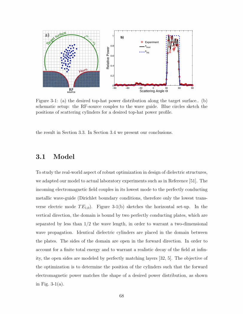
RFsource

30 ◦≤

θ ≤60 ◦

Horn

Targetsurfacea)

!90 !60 !30 0 30 60 900

0.2

0.4

0.6

0.8

1

Scattering Angle !

Rela

tive P

ow

er

Experiment

smod

sobj

b)

Figure 3-1: (a) the desired top-hat power distribution along the target surface.. (b)schematic setup: the RF-source couples to the wave guide. Blue circles sketch thepositions of scattering cylinders for a desired top-hat power profile.

the result in Section 3.3. In Section 3.4 we present our conclusions.

3.1 Model

To study the real-world aspect of robust optimization in design of dielectric structures,

we adapted our model to actual laboratory experiments such as in Reference [51]. The

incoming electromagnetic field couples in its lowest mode to the perfectly conducting

metallic wave-guide (Dirichlet boundary conditions, therefore only the lowest trans-

verse electric mode TE1,0). Figure 3-1(b) sketches the horizontal set-up. In the

vertical direction, the domain is bound by two perfectly conducting plates, which are

separated by less than 1/2 the wave length, in order to warrant a two-dimensional

wave propagation. Identical dielectric cylinders are placed in the domain between

the plates. The sides of the domain are open in the forward direction. In order to

account for a finite total energy and to warrant a realistic decay of the field at infin-

ity, the open sides are modeled by perfectly matching layers [32, 5]. The objective of

the optimization is to determine the position of the cylinders such that the forward

electromagnetic power matches the shape of a desired power distribution, as shown

in Fig. 3-1(a).

68

For the power distribution, the electromagnetic field over the entire domain, in-

cluding the scattering cylinders, is determined. As in the experimental measurements,

the frequency is fixed to f = 37.5 GHz [51]. Furthermore, the dielectric scatterers are

nonmagnetic and lossless. Therefore, stationary solutions of the Maxwell equations

are given through the two-dimensional Helmholtz equations, taking the boundary

conditions into account. This means, that only the z-component of the electric field

Ez can propagate in the domain. The magnitude of Ez in the domain is given through

the partial differential equation (PDE)

(∂x(µ−1ry∂x) + ∂y(µ

−1rx∂y))Ez − ω2

0µ0ε0εrzEz = 0 (3.1)

with µr the relative and µ0 the vacuum permeability. εr denotes the relative and ε0

the vacuum permittivity. Equation (3.1) is numerically determined using an evenly

meshed square-grid (xi, yi). The resulting finite-difference PDE approximates the field

Ez,i,j everywhere inside the domain including the dielectric scatterers. The imposed

boundary conditions (Dirichlet condition for the metallic horn and perfectly matching

layers) are satisfied. This linear equation system is solved by ordering the values of

Ez,i,j of the PDE into a column vector. Hence, the finite-difference PDE can be

rewritten as

L · Ez = b , (3.2)

where L denotes the finite-difference matrix, which is complex-valued and sparse. Ez

describes the complex-valued electric field, that is to be computed and b contains

the boundary conditions. With this, the magnitude of the field at any point of the

domain can be determined by solving the linear system of Eq. (3.2).

The power at any point on the target surface (x(θ), y(θ)) for an incident angle

θ is computed through interpolation using the nearest four mesh points and their

standard Gaussian weights W(θ) with respect to (x(θ), y(θ)) as

smod(θ) =W(θk)

2· diag(Ez) · Ez . (3.3)

69

!80 !60 !40 !20 0 20 40 60 800

0.2

0.4

0.6

0.8

1

Angle !

Re

lative

Po

we

r

USC Experiment

Fortran (res=0.4mm)

Matlab

Fortran (res=0.8mm)

!80 !60 !40 !20 0 20 40 60 800

0.2

0.4

0.6

0.8

1

Angle !

Re

lative

Po

we

r

USC Experiment

Fortran (res=0.4mm)

Matlab

Fortran (res=0.8mm)

Figure 3-2: Comparison between experimental data (circles) [51] and simulations ina) linear and b) logarithmic scale. The solid lines are simulation results for smallestmesh-size at ∆ = 0.4mm, and the dashed lines for ∆ = 0.8mm.

In the numerical implementation, we utilized the UMFPACK-library to LU de-

compose L as well as to solve the linear system directly [20]. Furthermore, our imple-

mentation uses the Goto-BLAS library for basic vector and matrix operations [27].

By exploiting the sparsity of L, we improved the efficiency of the algorithm signifi-

cantly. In fact, the solution of a realistic forward problem (∼ 70, 000×70, 000 matrix),

including 50 dielectric scatterers requires about 0.7 second on a commercially avail-

able Intel Xeon 3.4 GHz. Since the size of L determines the size of the problem,

the computational efficiency of our implementation is independent of the number of

scattering cylinders.

To verify this finite-difference technique for the power along the target surface

(radius = 60 mm from the domain center), we compared our simulations with exper-

imental measurements from Reference [51] for the same optimal arrangement of 50

dielectric scatterers (εr = 2.05 and 3.175± 0.025 diameter). Figure 3-2(a) illustrates

the good agreement between experimental and model data on a linear scale for an

objective top-hat function. The log-scale in Figure 3-2(b) emphasizes the relative in-

tensities of the side-lobes to the peak. This comparison also shows that the simulation

agrees well with experimental measurements only for a sufficiently small mesh-size of

∆ = 0.4mm ≤ λ0/20.

70

3.2 Robust Optimization Problem

By varying the positions of 50 scattering cylinders a top-hat power profile over the

target surface, as shown in Fig. 3-1(a), is sought. The desired objective function is

denoted by sobj. A cylinder configuration is given by a vector p ∈ R100. The actual

power profile along the target surface smod is computed using Equation (3.3). For

any given discretized angle θk and configuration p, a cost-functional J measures the

deviation of smod from sobj through

J(p) =m∑

k=1

|smod(θk)− sobj(θk)|2 . (3.4)

Therefore, the optimization problem is to minimize the area between sobj and smod.

This nominal optimization problem is given through

minp∈P

J(p). (3.5)

The minimization is with respect to the configuration vector p from a feasible set

P . Note that J(p) is not convex in p, and depends on p only over the linear system

L(p) · Ez(p) = b.

It needs to be emphasized that P is not a convex set. Instead, P is a 100 dimen-

sional hypercube containing a large number of non-empty infeasible subsets, which

represent non-physical configurations with overlapping cylinders. Defining these in-

feasible subsets explicitly through introducing constraints in the optimization problem

(3.5) is not practical due to the large number of constraints required. We took the

alternative approach of avoiding configurations with overlapping cylinders.

To consider possible implementation errors ∆p, the robust optimization problem

is defined as

minp∈P

max∆p∈U

J(p + ∆p). (3.6)

The uncertainty set U contains all the implementation errors, against which we want

to protect the design. Therefore, the robust optimization problem minimizes the worst

71

case cost under implementation error. These errors can arise due to misplacement

of the scattering cylinders in laboratory experiments or actual manufacturing of the

design.

We adopted a two-step strategy. In the first step, a good configuration to the

nominal optimization problem in Eq. (3.5) is found. This configuration is used as an

initial solution to the second step, since, with all factors being equal, a configuration

with a low nominal cost J(p) will have a low worst case cost max∆p∈U

J(p + ∆p). In

the second step, we iteratively update the configuration under evaluation with a more

robust configuration through a local shift until terminating conditions are satisfied.

This robust optimization algorithm does not assume any problem intrinsic structures.

We first discuss the nominal problem before we continue with the robust optimization

problem.

3.2.1 Nominal Optimization Problem

To solve the nominal Problem (3.5), we conducted a large number of random searches.

Because of the large dimensionality, a coarse-grained random search did not deliver

a significant and sufficiently fast improvement in minp∈P

J(p). Therefore, we developed

two alternative algorithms that efficiently returned a good solution to the nominal

optimization problem, as required in Step 1 of the robust optimization method.

Gradient Free Stochastic Algorithm

The first algorithm is adapted from the Simultaneous Perturbation Stochastic Ap-

proximation (SPSA) algorithm [55]. It relies only on function evaluations J(p). Under

general conditions, SPSA converges to a local minimum more efficiently, in expecta-

tion, than a gradient descent approach using finite-difference gradient estimates [55].

In iteration k, the algorithm seeks a better configuration along a direction dk

emanating from the configuration vector pk. The direction dk is a random vector

generated from a symmetric Bernoulli distribution where P (dki = ±1) = 1

2, ∀i, and is

deemed acceptable only when pk ± tkdk is feasible. Here, dki is the i-th coordinate of

72

dk and tk is a small positive scalar decreasing with k. Next, δk = J(pk+tkdk)−J(pk−

tkdk) is evaluated. Consequently, pk+1 is set to pk − αkδkdk, where αk is another

small positive scalar decreasing with k. Note that δk approximates the directional

gradient dk · ∇pJ(p = pk), if tk is small enough.

Modified Gradient Descent Algorithm

We computed the gradient of the cost-functional ∇pJ using the adjoint method.

In general, since the linear operator L maps the entire vector space Cn ↔ Cn, the

components of the cost-functional gradient can be determined from the equations (3.3)

and (3.4) through the adjoint equation as

∂J

∂pi

=

⟨g

∣∣∣∣∣ ∂E∂pi

⟩with g =

∂J

∂smod

∂smod∂E

(3.7)

= −

⟨h

∣∣∣∣∣ ∂L∂pi

E

⟩with L∗ · h = g.

Note, that L∗ is the adjoint operator to L, which was regularized in the implementa-

tion to warrant that J is differentiable. Therefore, in order to compute the gradient,

we have to solve the adjoint linear system L∗ · h = g. This equation has the same

structure and uses the same linear operator as the linear system for the function

evaluation in Eq. (3.2). Consequently, we exploited the structure of the problem and

utilize the LU decomposition of L for both the function and the gradient evaluation

at practically no additional computational cost.

For this optimization problem, standard gradient descent steps quickly led to in-

feasible configurations and terminated at solutions with high cost. Nevertheless, gra-

dient information is pertinent. To make use of it, we modified the standard algorithm

to avoid configurations with overlapping cylinders. These modifications are: (1) if a

gradient step leads to an infeasible configuration, the step size is repeatedly halved

until a threshold, or (2) otherwise, apply the gradient step only to those cylinders

that would not overlap. If the threshold is consistently breached, the algorithm ap-

proximates a coordinate descent algorithm which has similar convergence properties

73

0 1000 2000 3000 4000 50000

10

20

30

40

50

Iteration

J ×

10−

3

Gradient Free Stochastic AlgorithmModified Gradient Descent Algorithm

Figure 3-3: Performance comparison between the gradient free stochastic algorithmand the modified gradient descent algorithm on the nominal problem. Results showthat modified gradient descent is more efficient and converges to a better solution.

to standard gradient descent [37].

3.2.2 Nominal Optimization Results

The starting configuration for the optimization is obviously significant for the per-

formance. Due to the high-dimensional and non-convex response surface, a global

optimum can only be found through large-scale random searches, which is computa-

tionally exhaustive and, thus, beyond the scope of this work. Randomly generated

initial configurations often lead to overlapping cylinders. These infeasible arrange-

ments can only be overcome by human intervention, which we intended to omit. The

performance of a large number of regular PC-like structures with and without random

perturbation was simulated to obtain the best starting configuration. The inset of

Figure 3-3 illustrates this initial arrangement of the dielectric scattering cylinders, as

it appears to be an intuitively good structure as well.

We applied the gradient free stochastic algorithm and the modified gradient de-

scent algorithm to this initial configuration. Figure 3-3 shows that the modified gra-

dient descent algorithm reduces the objective function more efficiently. The gradient-

free algorithm took ∼ 2500 iterations to converge to an objective value of 0.0052. In

contrast, the modified gradient algorithm required ∼ 750 iterations to obtain con-

74

figurations with a cost lower than 0.0052; it eventually converged to a configuration

with a cost of 0.0032.

It is not surprising that the modified gradient descent algorithm outperforms the

gradient free stochastic algorithm. Note, that at each iteration step, the gradient

free algorithm uses two function evaluations and twice the time as compared to the

modified gradient descent algorithm. The gradient free algorithm does not decrease

the objective value monotonically, because, at any step, ck and αk may be too large.

Adopting a strategy employing smaller scalars can alleviate the spikes but increase the

overall time required to converge. Nevertheless, it is worthwhile to note the viability of

using a gradient free optimization approach, since an efficient cost-functional gradient

for such high-dimensional problems is not always available.

When the iteration count is high, both algorithms improve the objective value

monotonically, albeit very slowly because infeasible configurations are encountered

more often. Once the improvement rate went below a certain threshold, we terminated

the search and used the final nominal configuration as the initial configuration for the

robust optimization method.

3.2.3 Robust Local Search Algorithm

In laboratory experiments, implementation errors ∆p are encountered, when physi-

cally placing the cylinders. To include most of the errors, we define the uncertainty

set U such that the probability P (∆p ∈ U) = 99%. Consequently,

U = {∆p | ‖∆p‖2 ≤ Γ} , (3.8)

where ∆pi is assumed to be independently and normally distributed with mean 0 and

standard deviation 40µm, as observed in experiments [36]. We chose Γ to be 550µm.

Evaluating the worst cost under implementation errors involves solving an inner

maximization problem

max∆p∈U

J(p + ∆p) (3.9)

75

Γ

2Γ

pk

p1

p2

p3

p4

θθ

d∗

Figure 3-4: A 2-D illustration of the neighborhood {p | ‖p− p‖2 ≤ Γ}. The solidarrow indicates an optimal direction d∗ which makes the largest possible angle withthe vectors pi − p and points away from all bad neighbors pi.

which does not have a closed form solution. Thus, we can only find an estimate

of the worst case cost, Jmax(p), through efficient local searches. These searches are

conducted within the neighborhood N of a configuration p, defined as

N = {p | ‖p− p‖2 ≤ Γ} . (3.10)

This set is illustrated in Figure 2-7.

These searches form the first part of the robust local search algorithm. The

obtained worst case costs within N are used to find the next configuration with

a local move, which aims to improve the worst case cost. The local move forms

the second part of the robust local search algorithm. These two parts are repeated

iteratively until the termination conditions are met. Next, we discuss these two parts

in more detail.

Neighborhood Search

The local search within a neighborhoodN is conducted with several modified gradient

ascents. To ensure that N is explored thoroughly, an additional boundary penalty is

applied whenever an ascent step is near the boundary.

76

For this 100-dimensional problem, 101 gradient ascent sequences are carried out.

The first sequence starts from p while the remaining 100 sequences start from p+ Γ3ei,

if ∂J(p=p)∂pi

≥ 0 or from p− Γ3ei, otherwise. pi is a coordinate of p and ei denotes the

ith unit vector. A sequence is terminated when either a local maximum is obtained,

a configuration outside the neighborhood is visited, or a time limit is exceeded.

Finally, the results of all function evaluations up to iteration k are stored in a set

Hk and used to evaluate Jmax(pk).

Robust Local Move

In the second part of the robust local search algorithm, we update the configuration

pk such, that the previously discovered “bad” neighbors are excluded from the new

neighborhood N k+1. We define the set of these bad neighbors as

Mk = {p|p ∈ Hk,p ∈ N k, J(p) ≥ Jmax(pk)− σk}.

The cost factor σk governs the size of the set and may be changed within an iteration

to ensure a feasible move.

The problem of determining a good direction d, which points away from bad

neighbors, can be formulated as

mind,ε

ε

s.t. ‖d‖2 ≤ 1(p−pk

‖p−pk‖

)· d ≤ ε ∀p ∈Mk

ε ≤ 0.

(3.11)

Because the first constraint is a conic quadratic constraint and all others are linear,

this problem is a second order cone problem (SOCP), which can be solved efficiently

using both commercial and noncommercial solvers. The optimal solution of this

SOCP delivered a direction d∗ forming the maximum possible angle with all the

vectors p − pk, p ∈ Mk, as shown in Fig. 2-7. This angle is at least 90◦ due to the

constraint ε ≤ 0. However, if a good direction is not found, we reduce σk, reassemble

77

initial

configuration

final

configuration

1 10 20 30 40 50 60 65

6.5

6.4

6.3

6.2

6.1

6.0

3.3

3.2

Iteration

J×

10−

3

Jmax

Jnom

3.22

6.46

3.23

5.95

Figure 3-5: Performance of the robust local search algorithm. The worst case costfor the final configuration p65 is improved by 8%, while the nominal cost remainedconstant.

Mk, and solve the updated SOCP. The terminating condition is attained, when σk

decreases below a threshold.


As the first step of the robust optimization method, the nominal optimization also

decreases the worst case cost significantly. For the PC-like initial configuration (see

inset of Fig. 3-3), a worst case cost of Jmax = 0.05413 was estimated, whereas the

final nominal configuration delivered Jmax(p1) = 0.00646, as shown in Fig. 3-5. While

the nominal optimization primarily aims to reduce the nominal cost and increases the

robustness indirectly, only the robust local search algorithm directly minimizes the

worst case cost and, thus, improves the robustness further.

In the robust local search, the worst case cost at the terminating iteration step

65, Jmax(p65), was estimated with 110000 configurations in the neighborhood of p65.

78

As the iteration counts increase, the knowledge about the neighborhood grows and

the more robust configurations are discovered. Figure 3-5 shows the improvement

after 65 iterations of the robust local search algorithm. Here, the nominal cost of

the design remains practically constant, while the estimated worst case cost decreases

significantly. Overall, we observe a 90% improvement in robustness of the final design,

when compared to the initial PC-like structure.

Since we can only estimate the worst case cost by local searches, there is always

a chance for late discoveries of worst implementation errors. Therefore, the decrease

of the estimated worst case cost may not be monotonic.

3.3 Sensitivity Analysis

We have probed the neighborhood of p1 and p65 each with 10000 normally distributed

random perturbations. When the standard deviation of the perturbation is compa-

rable to the assumed implementation errors, p65 is up to 2% less sensitive as p1.

It is evident, that a 100-dimensional random sampling is computationally challeng-

ing, e.g., when estimating Jmax(p1), random sampling is far inferior to the multiple

gradient ascent method: the best estimate attained by the former with 30000 ran-

dom samples is 96% of the estimate obtained with only 3000 multiple gradient ascent

steps. Furthermore, a perturbation sensitivity analysis does not improve the worst

case performance. To the best of our knowledge, there is no practical approach that

improves sensitivities for a problem at such high dimensions. In contrast, our ap-

proach incorporates the widely used concept of probabilistic robustness through the

variable size of the uncertainty set U .

3.4 Conclusions

We have presented a novel robust optimization technique for electromagnetic scat-

tering problems and applied it to the optimization of aperiodic dielectric structures.

This generic method only assumes the capability of function evaluation. We have

79

demonstrated that using a modified gradient descent will increase the efficiency of

the robust algorithm significantly. However, if the function gradient is not accessible,

a gradient-free stochastic algorithm can be utilized to obtain a robust solution. The

application of our robust optimization method to improve the configuration of 50

dielectric cylinders showed that the final design configuration matches the shape of

the desired function whose top-hat maximum is at 30◦ ≤ θ ≤ 60◦. Since the prob-

lem is high-dimensional and highly non-convex, a global optimum can be estimated

only through local searches. While the deviation from an optimal solution (perfect

matching) is negligible, the robustness against implementation errors in laboratory

experiments or manufacturing increased by 8%. Furthermore, laboratory measure-

ments have verified our model [51].

The generic aspect of the presented method allows it to be employed in various

engineering problems in electromagnetics, in particular when function evaluation is

provided. Moreover, the demonstrated approach for the dielectric scattering structure

scales with frequency and can be applied to nano-photonic design to achieve novel

and desired functionalities.

80

Chapter 4


for Problems with Constraints

Constraints appear in many real-world problems. In a manufacturing application,

the number of items produced must exceed the quantity promised to the customers.

In cancer radiation therapy, a treatment plan must deliver the required radiation

dosage to a cancerous tumor, while sparing healthy organs. Due to the presence

of uncertainties, an otherwise “optimal” solution might violate critical constraints,

rendering it to become un-implementable. Therefore, for an optimization method to

be applicable to a wide range of real-world problems, it must admit constraints.

The robust local search technique for an unconstrained problem has been intro-

duced in Chapter 2. The proposed technique makes only one generic assumption:

the availability of a subroutine providing the cost and the gradient, when given a

design. Because only a simple assumption is made, the proposed method is much

more general than the robust models found in current literature, which assumes a

convex problem defined with linear, convex quadratic, conic-quadratic and semidef-

inite constraints [1, 4, 6, 8]. Consequently, the robust local search can be used for

many practical problems, convex or not. This applicability is demonstrated in Chap-

ter 3, when robust optimization in an actual engineering problem with a nonconvex

objective is carried out.

Our goal in this chapter is to generalize the robust local search further to ad-

81

mit constraints. The objective and the constraints can all be nonconvex. The basic

assumption on the availability of the cost and the gradient remains. In addition,

we assume the availability of the constraint value and the gradient of the constraint

value for every single constraint. This assumption is, again, a generic one. Therefore,

the proposed method remains applicable to a wide range of practical problems. Fur-

thermore, we consider how the efficiency of the algorithm can be improved, if some

constraints are simple, e.g. linear constraints.

To illustrate the technique more clearly, we start by considering a problem with

implementation errors only, before generalizing it to admit both implementation and

parameter uncertainties. The chapter is structured as follows.

Structure of the Chapter In Section 4.1, the robust local search is generalized to

handle a constrained problem with implementation errors. We also explore how the

efficiency of the algorithm can be improved, if some of the constraints have simple

structures, i.e. linear constraints. In Section 4.2, the algorithm is further generalized

to admit problems with implementation and parameter uncertainties. Application III

in Section 4.3 is designed to develop intuitions. Application IV in Section 4.4 considers

a similar problem as Application III, but with linear constraints. The robust local

search is shown to be more efficient when the simple constraints are exploited. The

final application, reported in Section 4.5, is an actual healthcare problem in Intensity

Modulated Radiation Therapy (IMRT) for cancer treatment. This problem has 85

decision variables.

82

4.1 Constrained Problem under Implementations

Errors


Consider the nominal optimization problem

minx

f(x)

s.t. hj(x) ≤ 0, ∀j,(4.1)

where both the objective function and the constraints may be nonconvex. To find

a good design which is robust against implementation errors in Problem (4.1), we

formulate the robust problem

minx

max∆x∈U

f(x + ∆x)

s.t. max∆x∈U

hj(x + ∆x) ≤ 0, ∀j,(4.2)

where ∆x are implementation errors. In this robust problem, we protect the design

against errors residing within an ellipsoidal uncertainty set U , given by

U := {∆x ∈ Rn | ‖∆x‖2 ≤ Γ} . (4.3)

Here, a larger scalar Γ indicates that larger perturbations will be taken into consider-

ations. A design is robust if and only if no constraint is violated, for any errors from

set U . Of all the robust designs, we seek one with the lowest worst case cost,

g(x) = max∆x∈U

f(x + ∆x). (4.4)

When a design x is implemented with errors from set U , the realized design falls

within the neighborhood,

N := {x | ‖x− x‖2 ≤ Γ} , (4.5)

83

x∆x1

∆x2

x1=x+∆x1

x2

Γ

θmax θmax

d∗

h2(x)>0

h1(x)>0

Figure 4-1: A 2-D illustration of the neighborhood N = {x | ‖x− x‖2 ≤ Γ} in thedesign space x. The shaded circle contains all the possible realizations when imple-menting x, when an error ∆x ∈ U is present. xi is a neighboring design (“neighbor”)which will be the outcome if ∆xi is the error. The shaded regions hj(x) > 0 containdesigns violating the constraints j. Note, that h1 is a convex constraint but not h2.As discussed in Chapter 2, if xi are neighbors with the highest nominal cost in the N(“bad neighbors”), d∗ is an update direction under the robust local search methodfor the unconstrained problem. d∗ makes the largest possible angle θ∗ with these badneighbors.

as illustrated in Fig. 4-1. x is a neighbor of x if it lies within the latter’s neighborhood.

Therefore, x is robust if and only if none of its neighbors violate any constraints.

Equivalently, there is any overlap between the neighborhood of x and the shaded

regions hj(x) > 0 in Fig. 4-1.

4.1.2 Robust Local Search for Problems with Constraints

When constraints do not come into play in the vicinity of the neighborhood of x, the

worst cost can be reduced iteratively, using the robust local search algorithm for the

unconstrained problem. Such a step, as indicated in Fig. 4-1, consists of

(i) Neighborhood Search: finding neighbors xi with the highest nominal costs in

N , and

(ii) Robust Local Move: taking a small step along an update direction d∗, which

84

points away from these bad neighbors, xi.

For further details of this algorithm, including methods to find these bad neighbors,

and the convex optimization approach to find the update direction efficiently, see

Section 2.2.

When constraints are present, the additional procedures required for the robust

local search algorithm include

(i) Neighborhood Search: Find neighbors xi that violates the constraints.

(ii) Check Feasibility Under Perturbations: If infeasible neighbors are found, x is

not feasible under perturbations. Else, it is deemed to be feasible.

(iii) Robust Local Move:

a. If x is not feasible under perturbations, find one that is, or

b. If x is feasible under perturbations, find one with a lower worst case cost.

With respect to an unconstrained problem, the additional procedures include:

(i) Neighborhood Search To determine if there are neighbors violating constraint

hj, the constraint maximization problem

max∆x∈U

hj(x + ∆x) (4.6)

is solved using multiple gradient ascents from different starting designs. Gradient

ascents are used because Problem (4.6) is a nonconvex optimization problem, in

general. We shall consider in Section 4.1.3 the case where hj is a simple constraint,

and consequently, Problem (4.6) can be solved using techniques more efficient than

multiple gradient ascents.

The implementation of the multiple gradient ascents can follow the generic neigh-

borhood search algorithm, described in Section 2.2, but with the cost function f(x)

replaced by the constraint functions hj(x). If a neighbor has a constraint value ex-

ceeding zero, for any constraint, it is recorded in a history set Y .

(ii) Check feasibility under perturbations If x has neighbors in the history

set Y , then it is not feasible under perturbations. Else, the algorithm treats x to be

85

feasible under perturbations.

(iii)a. Robust local move if x is not feasible under perturbations Because

constraint violations are more important than cost considerations, and we want the

algorithm to operate within the feasible region of robust problem, cost is ignored

when neighbors violating constraints are encountered.

To ensure that the new neighborhood does not contain neighbors in Y , an update

step along a direction d∗feas is taken. d∗feas is required to point away from these

neighbors. This is illustrated in Fig. 4-2, where yi denotes a neighbor violating

constraints and d∗feas makes the largest possible angle with all the vectors yi − x.

Such a d∗feas can be found by solving the SOCP

mind,β

β

s.t. ‖d‖2 ≤ 1,

d′(

yi−x‖yi−x‖2

)≤ β, ∀yi ∈ Y ,

β ≤ −ε.

(4.7)

As shown in Fig. 4-2, a sufficiently large step along d∗feas yields a robust design, take

for instance x + d∗feas.

(iii)b. Robust local move if x is feasible under perturbations When x is

feasible under perturbations, the update step is similar to that for an unconstrained

problem. However, ignoring designs violating constraints and lying just beyond the

neighborhood might lead to a non-robust design. To prevent that from happening,

such designs are considered when finding the update direction d∗cost, as illustrated in

Fig. 4-3.

86

x

y3 y4

y5y2

y1

d∗

feas

Figure 4-2: A 2-D Illustration of the robust local move, if x is non-robust. The uppershaded regions contain constraint-violating designs, including infeasible neighbors yi.Vector d∗feas, which points away from all yi can be found by solving SOCP (4.7). Thecircle with the broken circumference denotes the updated neighborhood of x + d∗feas,which is robust.

xy1

y2

x1 x2

x3

d∗

cost

Figure 4-3: A 2-D Illustration of the robust local move when x is robust. xi denotesa bad neighbor with high nominal cost, while yi denotes an infeasible neighbor lyingjust outside the neighborhood. By solving SOCP (4.8), d∗cost, a vector which pointsaway from xi and yi, can be found. The neighborhood of x + d∗cost contains neitherthe designs with high cost nor the infeasible designs.

87

The update direction d∗cost can be found by solving the SOCP

mind,β

β

s.t. ‖d‖2 ≤ 1,

d′(

xi−x‖xi−x‖2

)≤ β, ∀xi ∈M,

d′(

yi−x‖yi−x‖2

)≤ β, ∀yi ∈ Y+,

β ≤ −ε,

(4.8)

where M contains neighbors with cost that is among the highest within the neigh-

borhood, and Y+ is the set of known infeasible designs lying in the slightly enlarged

neighborhood N+,

N+ := {x | ‖x− x‖2 ≤ (1 + δ)Γ} , (4.9)

δ being a small positive scalar.

Since x is robust, there are no infeasible designs in the neighborhood N . There-

fore, if there are any infeasible designs in Y+, they lie at a distance between Γ and

(1 + δ)Γ. With δ being small, these designs are lying just beyond the neighborhood,

as illustrated in Fig. 4-3.

Termination criteria We shall first define the robust local minimum for a problem

with constraints:

Definition 3

x∗ is a robust local minimum for the problem with constraints if

(i) Feasible Under Perturbations

x∗ remains feasible under perturbations,

hj(x∗ + ∆x) ≤ 0, ∀j,∀∆x ∈ U , (4.10)

and

88

(ii) No Descent Direction

there are no improving direction d∗cost at x∗.

Given the above definition, we can only terminate in Step (iii)b where x∗ is feasible

under perturbations. Furthermore, for there to be no direction d∗cost at x∗, it must be

surrounded by neighbors with high cost, and infeasible designs in N+.

4.1.3 Enhancements when Constraints are Simple

In the context of the robust local search, a constraint is simple when the corresponding

constraint maximization problem (4.6) is convex. When Problem (4.6) is convex, it

can be solved with techniques that are more efficient than multiple gradient ascents.

Moreover, it is possible to obtain (i) the global optimizer ∆x∗j to the Prob. (4.6), (ii)

the maximum constraint value attained in the neighborhood,

hrobj (x) = max

∆x∈Uhj(x + ∆x) = hj(x + ∆x∗j),

and consequently, (iii) confirmation whether any neighbor of x violate constraint j.

Many constraints lead to a convex constraint maximization problem (4.6), includ-

ing x ≥ 0, linear or convex quadratic constraints. Table 4.1 summarizes the procedure

required to solve Problem (4.6). Note, that in Problem (4.6), x is a constant and ∆x

are the only variables.

hi(x) Problem (4.6) Effort requireda′x + b a′x + Γ‖a‖2 + b ≤ 0 Computations

x′Qx + 2b′x + c, Single trust region Solving a SDP in the worst caseQ symmetric problem1

−hi is convex Convex problem Just 1 gradient ascent is requiredhi is a polynomial Polynomial problem May be solved using

Gloptipoly [29] to a high accuracy

Table 4.1: Efforts required to solve Prob. (4.6)

The possible improvements to the robust local search are:

1 max∆x∈U

∆x′Q∆x + 2(Qx + b)′∆x + xQ′x + 2b′x + c,

89

(i) Neighborhood Search: Solve Problem (4.6) with method stated in Table 4.1

and not multiple gradient ascents, which requires more computation effort in

general.

(ii) Check Feasibility Under Perturbations: If hrobj (x) > 0, x is not feasible under

perturbations.

(iii) Robust Local Move: To not violate hj in the new neighborhood, the direction

should be chosen such that

d′feas∇xhrobj (x) < β‖∇xh

robj (x)‖2

and

d′cost∇xhrobj (x) < β‖∇xh

robj (x)‖2

in SOCP (4.7) and SOCP (4.8), respectively. Note, that ∇xhrobj (x) = ∇xh(x +

∆x∗j). This can be evaluated easily.

In particular, if hj is a linear constraint,

hrobj (x) = a′x + Γ‖a‖2 + b ≤ 0

is same for all x. Consequently, we can replace the constraint max∆x∈U

hj(x + ∆x) =

max∆x∈U

a′(x + ∆x) ≤ 0 with its robust counterpart hrobj (x). hrob

j (x) is a constraint on x

without any uncertainties, as illustrated in Fig. 4-4.

4.1.4 Constrained Robust Local Search Algorithm

Bringing all these procedures together, the constrained robust local search algorithm

for Problem (4.2) is:

In Steps 3(i) and 3(ii), tk is the minimum distance chosen such that the undesirable

designs are excluded from the neighborhood of the new iterate xk+1. Finding tk

requires solving a simple geometric problem. For more details, refer to Section 2.2.2.

90

x

y1

y2

∇xhrob(x)

d∗

feas

Figure 4-4: A 2-D Illustration of the neighborhood when one of the violated constraintis a linear function. The shaded region in the upper left hand corner denotes theinfeasible region due a linear constraint. Because x has neighbors violating the linearconstraint, x lies in the infeasible region of its robust counterpart, denoted by theregion with the straight edge but of a lighter shade. yi denotes neighbors violatinga nonconvex constraint. The vector d∗feas denotes a direction which would reducethe infeasible region within the neighborhood. It points away from the gradient ofthe robust counterpart, ∇xh

rob(x) and all the bad neighbors yi. It can be found bysolving a SOCP. The circle with the dashed circumference denotes the neighborhoodof the design x + d∗feas, where no neighbors violate the two constraints.

91

Algorithm 3 Constrained Robust Local Search

Step 0. Initialization: Set k := 1. Let x1 be an arbitrary decision vector.Step 1. Neighborhood Search:

i. Find neighbors with high cost by applying n+ 1 gradient ascents on theinner maximization problem (2.12) where n is the dimension of x. Formore details, refer to Section 2.2.1. Record all neighbors evaluated andtheir costs in history set Hk, together with Hk−1.

ii. Let J be the set of constraints with convex constraint maximizationProblem (4.6) that are convex. Find optimizer ∆x∗j and highest con-straint value hrob

j (xk), for all j ∈ J , using methods as stated in Ta-ble. 4.1. Let J ⊆ J be the set of violated constraints violated underperturbations.

iii. For every constraint j 6∈ J , find infeasible neighbors by applying n + 1gradient ascents on Problem (4.6), with x = xk. Record all infeasibleneighbors in history set Yk, together with set Yk−1.

Step 2. Check Feasibility Under Perturbations: xk is not feasible under perturba-

tions if either Yk or J is not empty.Step 3. Robust Local Move:

i. If xk is not feasible under perturbations, solve SOCP (4.7) with ad-ditional constraints d′feas∇xh

robj (xk) < β‖∇xh

robj (xk)‖2, for all j ∈ J .

Find direction d∗feas and set xk+1 := xk+1 + tkd∗feas.

ii. If xk feasible under perturbations, solve SOCP (4.8) to find a directiond∗cost. Set xk+1 := xk+1 + tkd∗feas. If no direction d∗cost exists, reduce σ; ifσ is below a threshold, terminate.

92

4.1.5 Practical Considerations

Implementation In a practical implementation, some possible modifications to

this algorithm include:

• Using less than n+1 gradient ascents during the neighborhood search to reduce

the computational effort.

• Using bounds or other techniques to identify constraints that would not be

violated in the neighborhood, and excluding them when looking for infeasible

neighbors.

Difficult Feasibility Problem Even without uncertainties, a problem with non-

convex constraints can be a challenging one. Therefore, in a difficult problem, the

feasible region for the robust problem (4.2) might be small, not connected, or even

non-existent. In this case, the algorithm can be trapped within an endless loop, try-

ing to find designs that are feasible under perturbations. If this is encountered, the

robust local search has to be started from an alternate design.

4.2 Generalization to Include Parameter Uncer-

tainties


Consider the nominal problem:

minx

f(x, p)

s.t. hj(x, p) ≤ 0, ∀j,(4.11)

where p ∈ Rm is a coefficient vector of problem parameters. For our purpose, we can

restrict p to parameters with perturbations only. For example, if Problem (4.11) is

given by

minx

4x31 + x2

2 + 2x21x2

s.t. 3x21 + 5x2

2 ≤ 20,

93

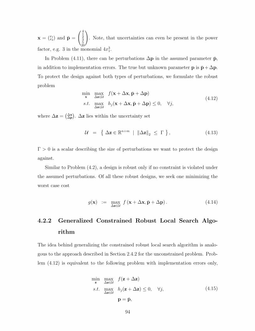
x = (x1x2) and p =

( 4123520

). Note, that uncertainties can even be present in the power

factor, e.g. 3 in the monomial 4x31.

In Problem (4.11), there can be perturbations ∆p in the assumed parameter p,

in addition to implementation errors. The true but unknown parameter p is p+ ∆p.

To protect the design against both types of perturbations, we formulate the robust

problem

minx

max∆z∈U

f(x + ∆x, p + ∆p)

s.t. max∆z∈U

hj(x + ∆x, p + ∆p) ≤ 0, ∀j,(4.12)

where ∆z =(∆x∆p

). ∆z lies within the uncertainty set

U ={

∆z ∈ Rn+m | ‖∆z‖2 ≤ Γ}, (4.13)

Γ > 0 is a scalar describing the size of perturbations we want to protect the design

against.

Similar to Problem (4.2), a design is robust only if no constraint is violated under

the assumed perturbations. Of all these robust designs, we seek one minimizing the

worst case cost

g(x) := max∆z∈U

f (x + ∆x, p + ∆p) . (4.14)

4.2.2 Generalized Constrained Robust Local Search Algo-

rithm

The idea behind generalizing the constrained robust local search algorithm is analo-

gous to the approach described in Section 2.4.2 for the unconstrained problem. Prob-

lem (4.12) is equivalent to the following problem with implementation errors only,

minz

max∆z∈U

f(z + ∆z)

s.t. max∆z∈U

hj(z + ∆z) ≤ 0, ∀j,

p = p,

(4.15)

94

where z = (xp). Consequently, the necessary modifications to Algorithm 4.1.4 are:

(i) Neighborhood Search : Given x, z =(xp

)is the decision vector. The neighbor-

hood is

N := {z | ‖z− z‖2 ≤ Γ} ={(xp) |

∥∥x−xp−p

∥∥2≤ Γ

}. (4.16)

(ii) Robust Local Move : Let d∗ =(

d∗xd∗p

)be a update direction in the z space.

Because p is not a decision vector but a given system parameter, the algorithm

has to ensure that p = p is satisfied at every iterate. Thus, d∗p = 0.

When finding the update direction, the condition dp = 0 must be included in

either of SOCP (4.7) and SOCP (4.8). For example, in the case where z is not

feasible under perturbations, the SOCP is

mind=(dx,dp),β

β

s.t. ‖d‖2 ≤ 1,

d′ (zi − z) ≤ β‖zi − z‖2, ∀yi ∈ Y ,

d′∇zhrobj (z) < β‖∇zh

robj (z)‖2, ∀j ∈ J ,

dp = 0,

β ≤ −ε.

Yk is the set of infeasible designs in the neighborhood. This problem reduces to

the following:

mindx,β

β

s.t. ‖dx‖2 ≤ 1,

d′x (xi − x) ≤ β‖zi − z‖2, ∀yi ∈ Y ,

d′x∇xhrobj (z) < β‖∇zh

robj (z)‖2, ∀j ∈ J ,

β ≤ −ε.

(4.17)

A similar approach is carried out for the case where z is robust. Consequently,

both d∗feas and d∗cost satisfy p = p at every iteration, as illustrated in Fig. 4-5.

95

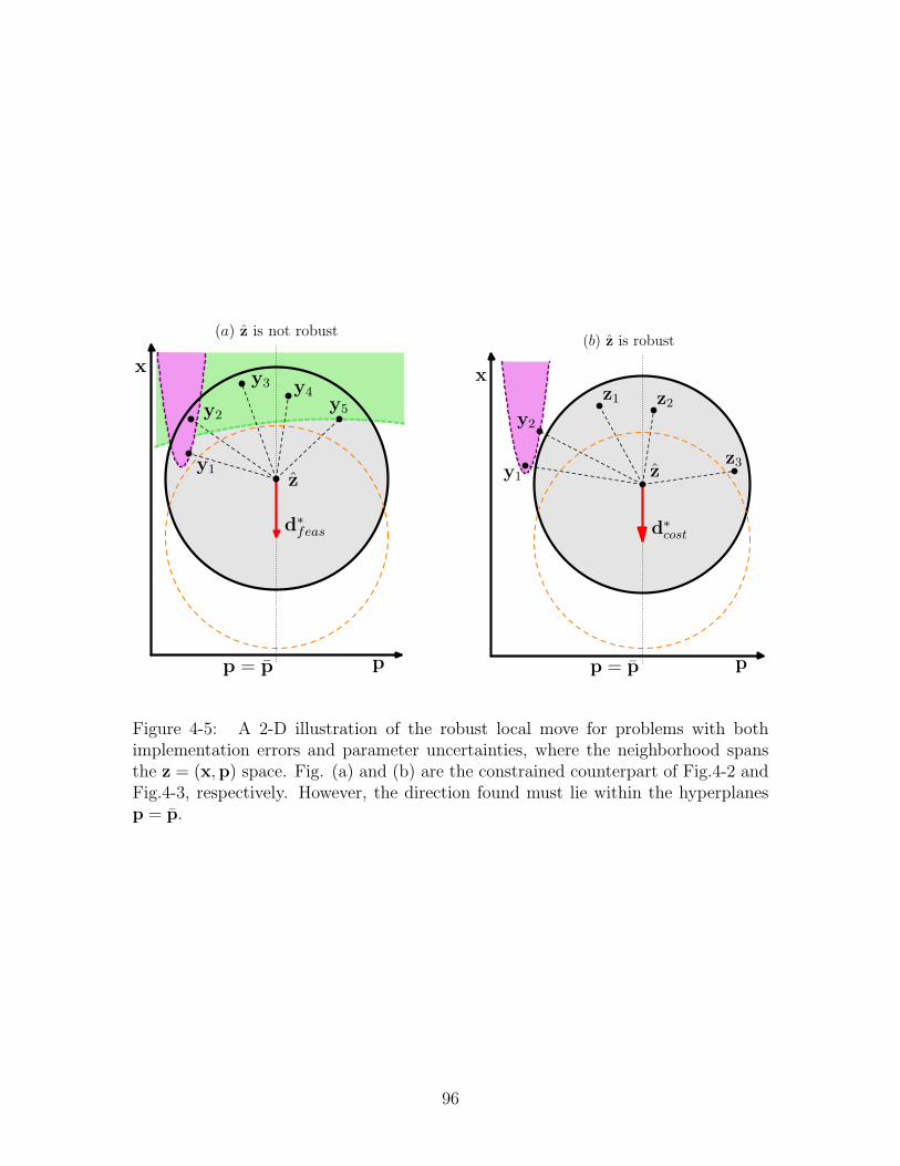
p

x

z

y3 y4

y5y2

y1

d∗

feas

p = p

(a) z is not robust

zy1

y2

z1 z2

z3

p

x

d∗

cost

p = p

(b) z is robust

Figure 4-5: A 2-D illustration of the robust local move for problems with bothimplementation errors and parameter uncertainties, where the neighborhood spansthe z = (x,p) space. Fig. (a) and (b) are the constrained counterpart of Fig.4-2 andFig.4-3, respectively. However, the direction found must lie within the hyperplanesp = p.

96

We have thus arrived at the constrained robust local search algorithm for Prob-

lem 4.12 with both implementation errors and parameter uncertainties:

Algorithm 4 Generalized Constrained Robust Local Search

Step 0. Initialization: Set k := 1. Let x1 be an arbitrary decision vector.Step 1. Neighborhood Search: Same as Step 1 in Algorithm 4.1.4 but over the neigh-

borhood (4.16).Step 2. Check Feasibility under Perturbations: zk, and equivalently xk, is feasible

under perturbations if Yk and J k are empty.Step 3. Robust Local Move:

i. If xk is not feasible under perturbations, find a direction d∗feas by solving

SOCP (4.17) with z = zk. Set xk+1 := xk+1 + tkd∗feas.ii. If x is feasible under perturbations, solve the SOCP

mindx,β

β

s.t. ‖dx‖2 ≤ 1,

d′x(xi − xk

)≤ β

∥∥(xi−xk

pi−p

)∥∥2, ∀zi ∈Mk, zi = (xi

pi) ,

d′x(xi − xk

)≤ β

∥∥(xi−xk

pi−p

)∥∥2, ∀yi ∈ Yk

+,yi = (xipi) ,

d′x∇xhrobj (zk) < β‖∇zh

robj (zk)‖2, ∀j ∈ J+,

β ≤ −ε,

(4.18)

to find a direction d∗cost. Yk+ is the set of infeasible designs in the enlarged

neighborhood N k+, Eq. 4.9. J+ is the set of constraints which are not

violated in the neighborhood of x, but are violated in the slightly enlargedneighborhood N+. Set xk+1 := xk+1 + tkd∗feas. If no direction d∗cost exists,reduce σ; if σ is below a threshold, terminate.

We are now ready to apply the robust local search.

4.3 Application III: Problem with Polynomial Cost

Function and Constraints


The first problem in this chapter was obtained by adding two constraints to Applica-

tion I. The resulting problem is sufficiently simple, so as to develop intuition into the

97

algorithm. Consider the nominal problem

minx,y

fpoly(x, y)

s.t. h1(x, y) ≤ 0,

h2(x, y) ≤ 0,

(4.19)

where


−10y − 74.8y3 + 56.9y2 − 4.1xy − 0.1y2x2 + 0.4y2x+ 0.4x2y

h1(x, y) = (x− 1.5)4 + (y − 1.5)4 − 10.125,

h2(x, y) = −(2.5− x)3 − (y + 1.5)3 + 15.75.

Given implementation errors∥∥∆ =

(∆x∆y

)∥∥2≤ 0.5, the robust problem is

minx,y

max‖∆‖2≤0.5

fpoly(x+ ∆x, y + ∆y)

s.t. max‖∆‖2≤0.5

h1(x+ ∆x, y + ∆y) ≤ 0,

max‖∆‖2≤0.5

h2(x+ ∆x, y + ∆y) ≤ 0.

(4.20)

There are no practical ways to solve such a robust problem, given today’s technol-

ogy [34]. If the relaxation method for polynomial optimization problems [29] is used,

Problem (4.20) leads to a large polynomial SDP problem which cannot be solved in

practice today [33, 34]. The nominal and the estimated worst cost surface is shown

in Fig. 4-6.


The nonconvex cost surface and the feasible region of Problem (4.19) are shown in

Figure 4-7(a). Note, that the feasible region is not convex, because h2 is not a convex

98

−1 0 1 2 3

0

1

2

3

4

x

y

(a) Nominal Cost

−20

0

20

40

60

80

100

−1 0 1 2 3

0

1

2

3

4

x

y


0

50

100

150

200

250

300

350

Figure 4-6: Contour plot of nominal cost function fpoly(x, y) and the estimated worstcase cost function gpoly(x, y) in Application I.

constraint. Let gpoly(x, y) be the worst case cost function,

gpoly(x, y) := max‖∆‖2≤0.5

fpoly(x+ ∆x, y + ∆y).

Figure 4-7(b) shows the worst case cost estimated using sampling on the cost surface

fpoly. In the robust problem (4.20), we seek the design minimizing gpoly(x, y), among

all the designs with a neighborhood lying within the unshaded region. An example

of such a design is point C in Fig. 4-7(b).

Applying the constrained robust local search Two separate robust local searches

were carried out from initial designs A and B. The algorithm found designs that are

feasible under perturbations and with much lower worst case costs in both instances,

as shown in Fig. 4-8.

However, it converged to different robust local minima in the two instances, as

shown in Fig. 4-9. The presence of multiple robust local minima is not surprising

because gpoly(x, y) is nonconvex. Figure 4-9 also show that both robust local minima

I and II satisfy the terminating conditions stated in Section 4.1.2:

(i) Feasible under Perturbations: Both their neighborhoods do not overlap with the

shaded regions.

99

(a) Nominal Cost

x

y

0 0.5 1 1.5 2 2.5 3

0

1

2

3


x

y

B

A

C

0 0.5 1 1.5 2 2.5 3

0

1

2

3

Figure 4-7: Contour plot of (a) the nominal cost function fpoly(x, y) and (b) theestimated worst case cost function gpoly(x, y) in Application IV. The shaded regionsdenote designs which violate at least one of the two constraints, h1 and h2. Whileboth point A and point B are feasible, they are not feasible under perturbations,because they have infeasible neighbors. Point C, on the other hand, is feasible underperturbations.

100

(a) Descent Path (from Point A)

x

y

0 1 2 3

0

1

2

3

0 20 40 60 80 1005

10

15

20

25

30

35

IterationE

stim

ated

Wor

st C

ase

Cos

t

(b) Cost vs. Iteration (from Point A)

WorstNominal

(c) Descent Path (from Point B)

x

y

0 1 2 3

0

1

2

3

0 10 20 30 40 500

50

100

150

Iteration

Est

imat

ed W

orst

Cas

e C

ost

(d) Cost vs. Iteration (from Point B)

WorstNominal

Figure 4-8: Performance of the robust local search algorithm in Application IV from2 different starting points A and B. The circle marker and the diamond markerdenote the starting point and the final solution, respectively. (a) The contour plotshowing the estimated surface of the worst case cost, gpoly(x, y). The descent pathtaken to converge at the robust solution is shown. (b) From starting point A, thealgorithm reduces both the worst case cost and the nominal cost. (c),(d) From anotherstarting point B, the algorithm converged to a different robust solution, which has asignificantly smaller worst case cost and nominal cost.

101

(ii) No improving direction d∗cost: Both designs are surrounded by bad neighbors

and infeasible designs lying just outside their respective neighborhoods. For

robust local minimum II, note that the bad neighbors lie on the same contour

line even though they are apart.

4.4 Application IV: Polynomial Problem with Sim-

ple Constraints

In Section 4.1.3, we argued that the robust local search can be more efficient if simple

constraints, such as linear constraints, are replaced by their robust counterparts. The

objective of this example is to show this improvement.


The nominal problem is

minx,y

fpoly(x, y)

s.t. h1(x, y) ≤ 0,

h2(x, y) ≤ 0,

(4.21)

where


−10y − 74.8y3 + 56.9y2 − 4.1xy − 0.1y2x2 + 0.4y2x+ 0.4x2y,

h1(x, y) = 0.6x− y + 0.17,

h2(x, y) = −16x− y − 3.15.

Given the uncertainty set U ={∆ =

(∆x∆y

)| ‖∆‖2 ≤ 0.5

}, the robust problem is

minx,y

max∆∈U


s.t. max∆∈U

h1(x+ ∆x, y + ∆y) ≤ 0

max∆∈U

h2(x+ ∆x, y + ∆y) ≤ 0.

(4.22)

102

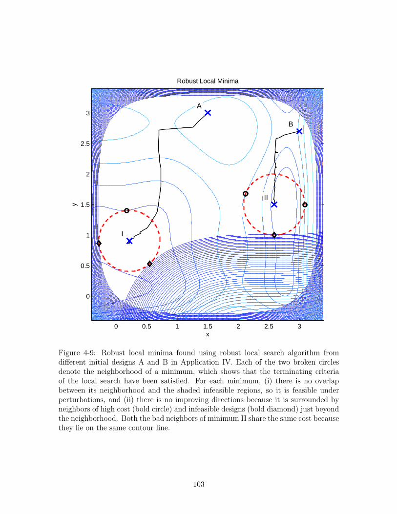
B

II

A

I

Robust Local Minima

x

y

0 0.5 1 1.5 2 2.5 3

0

0.5

1

1.5

2

2.5

3

Figure 4-9: Robust local minima found using robust local search algorithm fromdifferent initial designs A and B in Application IV. Each of the two broken circlesdenote the neighborhood of a minimum, which shows that the terminating criteriaof the local search have been satisfied. For each minimum, (i) there is no overlapbetween its neighborhood and the shaded infeasible regions, so it is feasible underperturbations, and (ii) there is no improving directions because it is surrounded byneighbors of high cost (bold circle) and infeasible designs (bold diamond) just beyondthe neighborhood. Both the bad neighbors of minimum II share the same cost becausethey lie on the same contour line.

103

Because hj are linear, they have robust counterparts

hrob1 (x, y) = 0.6x− y + 0.17 + 0.5831 ≤ 0,

hrob2 (x, y) = −16x− y − 3.15 + 8.0156 ≤ 0,

as described in Table 4.1. To derive hrobj , take hrob

1 for example:

max∆∈U

0.6(x+ ∆x)− (y + ∆y) + 0.17 = 0.6x− y + 0.17 + 0.5 ‖(0.6−1)‖2

= 0.6x− y + 0.17 + 0.5831.

Therefore, Problem (4.22) is equivalent to the problem

minx,y

max∆∈U


s.t. hrob1 (x, y) ≤ 0

hrob2 (x, y) ≤ 0.

(4.23)

We applied the robust local search on both Problem (4.22) and Problem (4.23),

using the same initial design. The difference in performance is then compared. The

nominal and the estimated worst cost surface is shown in Fig. 4-6.


The algorithm reduced the worst case cost significantly and converged to the same

robust local minimum in both cases. This is shown in Fig. 4-10(a),(b). Fig. 4-10(b)

also shows that the reduction in worst case cost is faster when solving Problem (4.23).

The most significant difference was the time required to terminate. While the

algorithm took 3600 seconds to terminate for Problem (4.22), it terminated in only

96 seconds when applied to Problem (4.23), which involves robust counterparts.

Fig. 4-10(c) shows that the robust local minimum satisfies the terminating condi-

tions stated in Section 4.1.2:

(i) Design is feasible under perturbations: The robust local minimum lies on line

104

(a) Descent Path

x

y

0 1 2 3

0

1

2

3

4

0 20 40 60 80 100

10

15

20

25

30

Time/seconds

Est

imat

ed W

orst

Cas

e C

ost

(b) Efficiency Gained from using Robust Counterparts

UsingNot Using

(c) Termination Conditions Attained

x

y

∇ hrob1

(x,y)

h1(x,y) > 0

∇ hrob2

(x,y)

h2(x,y) > 0

−0.2 0 0.2 0.4 0.6 0.8 1

0

0.2

0.4

0.6

0.8

1

1.2

1.4

Figure 4-10: Performance of the robust local search algorithm applied to Prob-lem (4.22)-(4.23). (a) In both instances, the algorithm takes a similar descent pathand converge at the same robust local minimum. (b) The robust local search is moreefficient when applied on the problem formulated with robust counterparts. (c) Ter-mination criteria attained by the robust local minimum (x∗, y∗), which is indicated bythe cross marker. The solid line parallel to the shaded infeasible regions hj(x, y) > 0denote the line hrob

j (x, y) = 0, for j = 1, 2. (x∗, y∗) is robust because it does not vio-late the constraints hrob

j (x, y) ≤ 0. From (x∗, y∗), there are also no vectors pointingaway from the bad neighbor (bold circle) and the directions ∇hrob

j (x, y).

105

intersection hrobj (x, y) = 0, j = 1, 2. Since the constraints are not violated, the

design is feasible under perturbations. The robustness is also confirmed by the

lack of overlapping between its neighborhood and the shaded regions.

(ii) No improving direction d∗cost: There are no directions (vectors) pointing away

from the bad neighbor, and making angle larger than 90◦ with the gradients,

∇hrobj (x, y).

4.5 Application V: A Problem in Intensity Mod-

ulated Radiation Therapy (IMRT) for Cancer

Treatment

Radiation therapy is a key component in cancer treatment today. In this form of

treatment, ionizing radiation is directed onto cancer cells with the objective of de-

stroying them. Unfortunately, healthy and non-cancerous cells are exposed to the

destructive radiation as well since cancerous tumors are embedded within the pa-

tient’s body. Even though most healthy cells can repair themselves, an important

objective behind the planning process is to minimize the total radiation received by

the patient (“objective”), while ensuring that the tumor is subjected to a sufficient

level of radiation (“constraints”).

Most radiation oncologists adopt the technique of Intensity Modulated Radiation

Therapy (IMRT) [10]. In IMRT, the dose distribution is controlled by two set of

decisions. First, instead of a single beam, multiple beams of radiation are directed

onto the tumor, from different angles. This is illustrated in Fig. 4-11 and accomplished

using a rotatable oncology system such as the one shown in Fig. 4-12. Furthermore,

the intensity of each individual beam can be modulated using multi-leaf collimators

such as the one shown in Fig. 4-13. The beam passes through the gap made by

multiple layers of collimators. By sliding the collimators, the shape of the gap and,

consequently, the radiation dosage distribution can be controlled.

Fig. 4-14 shows the schematic of a IMRT treatment. In the example illustrated,

106

ionizing

radiationnormal

cells

cancer

cells

Figure 4-11: Multiple ionizing radiation beams are directed at cancerous cells withthe objective of destroying them.

Figure 4-12: A typical oncology system used in IMRT. The radiation beam can bedirected onto a patient from different angles, because the equipment can be rotatedabout an axis. Credits to: Rismed Oncology Systems, http://www.rismed.com/ sys-tems/tps/IMG 2685.JPG, April 15, 2007.

107

Figure 4-13: A beam’s eye-view of the multi-leaf collimators used for beam modulationin IMRT. The radiation beam passes through the gap made by multiple layers ofcollimators. By sliding the collimators, the shape of the gap is changed. Consequently,the distribution of the radiation dosage introduced to the body can be controlled.Credits to: Varian Medical Systems, http:// www.varian.com, April 15, 2007.

radiation is directed from three angles. Moreover, there are three beamlets in each

beam and their intensities are controllable as well. By choosing the beam angles

and the beamlet intensities (“decision variables”), it is desirable to make the treated

volume conform as closely as possible to the target volume, thereby minimizing radia-

tion dosage on organ-at-risk (OAR) and normal tissues. In a case of prostate cancer,

for instance, the target volume would include the prostate glands, while the OAR

would include the rectum, the spine and the kidneys. Without careful planning, the

treatment can easily damage these organs-at-risk and reduce a patient’s quality of

life subsequently, even if the cancer has been addressed.

Optimization Problem We obtained our optimization model through a joint re-

search project with the Massachusetts General Hospital. In the model, all the affected

body tissue are divided into discrete volume elements called a voxel v [21]. The voxels

belong to three sets. They are, namely,

• T : the set of tumor voxels, |T | = 145.

108

Figure 4-14: Schematic of IMRT. Radiation is delivered on the tumor from threedifferent angles. From each angle, a single beam is made up of 3 beamlets, denotedby the arrows. Credits to: Thomas Bortfeld, Massachusetts General Hospital.

• O: the set of organ-at-risk voxels, |O| = 42.

• N : the set of normal tissue voxels, |N | = 1005.

Let the set of all voxels be V . Therefore, V = T ∪ O ∪ N and |V| = 1192; there are

a total of 1192 voxels.

In our application example, there are five beams, each from a different angle. In

each beam, there are sixteen beamlets. Let θ ∈ R5 be the vector of beam angles and

I be the set of beams. In addition, let Bi be set of beamlets b belonging to beam

i, i ∈ I. Finally, let xbi be the intensity of beamlet b, b ∈ Bi, and x ∈ R16×5 be the

vector of beamlet intensities,

x =

x1

1

...x16

1

x12

...x16

5

. (4.24)

Let Dbv(θi) be the radiation dosage in voxel v introduced by beamlet b from beam

i when the beamlet has an intensity of 1, i.e. xbi = 1. Thus,

∑i

∑b

Dbv(θi)x

bi denotes

the total dosage in voxel v under a treatment plan (θ,x). Therefore, the objective

is to minimize a weighted sum of the radiation dosage in all voxels, while ensuring

109

that (i) a minimum dosage lv is delivered to each tumor voxel v ∈ T , and (ii) the

dosage in each voxel v does not exceed an upper limit uv. Consequently, the nominal

optimization problem is

minx,θ

∑v∈V

∑i∈I

∑b∈Bi

cvDbv(θi)x

bi

s.t.∑i∈I

∑b∈Bi

Dbv(θi)x

bi ≥ lv, ∀v ∈ T ,∑

i∈I

∑b∈Bi

Dbv(θi)x

bi ≤ uv, ∀v ∈ V ,

xbi ≥ 0, ∀b ∈ Bi,∀i ∈ I,

(4.25)

where term cv is the penalty of a unit dose in voxel v. A much higher penalty is set

for a voxel in the OAR versus a voxel in the normal tissue.

Note, that if θ is given, Problem (4.25) reduces to an LP and the optimal intensities

x∗(θ) can be found efficiently. However, the problem is nonconvex in θ because varying

a single θi changes Dbv(θi) for all voxel v and for all b ∈ Bi.

Let φ be the angle of a single beam. To getDbv(φ), the values at φ = 0◦, 2◦, . . . , 358◦

were derived using CERR, a numerical solver for radiotherapy research [21]. Subse-

quently for a given θ, Dbv(θ) is obtained using a linear interpolation using these derived

values:

Dbv(θ) =

φ− θ + 2◦

2◦·Db

v(φ) +θ − φ

2◦·Db

v(φ+ 2◦) (4.26)

where φ = 2b θ2c. It is not practical to use the numerical solver to compute Db

v(θ)

directly during optimization because the derivation takes too much time.

Model of Uncertainty When a design (θ,x) is implemented, the realized design is

of the form (θ+∆θ,x⊗(1±δ)), where ⊗ refers to an element-wise multiplication. The

sources of errors include equipment limitation, the difference in the patient’s posture

when measuring and irradiating, and minute body movements. The perturbations

110

are estimated to be normally and independently distributed:

δbi ∼ N (0, 0.01) ,

∆θi ∼ N(0, 1

3

◦).

(4.27)

Under the robust optimization approach, we define the uncertainty set

U =

δ

0.03

∆θ

|

∥∥∥∥∥∥δ

0.03

∆θ

∥∥∥∥∥∥2

≤ Γ

. (4.28)

The factor 0.03 is introduced to compensate for the difference in error magnitudes.

Numerous robust designs will be obtained using different values of Γ. These designs

will then be compared using 10,000 samples drawn from the distribution in Eq. (4.27).

Given the uncertainty set Eqn.(4.28), the corresponding robust problem is

minx,θ

max(δ,∆θ)∈U

∑v∈V

∑i∈I

∑b∈Bi

cvDbv(θi + ∆θi)x

bi(1 + δb

i )

s.t. min(δ,∆θ)∈U

∑i∈I

∑b∈Bi

Dbv(θi + ∆θi)x

bi(1 + δb

i ) ≥ lv, ∀v ∈ T

max(δ,∆θ)∈U

∑i∈I

∑b∈Bi

Dbv(θi + ∆θi)x

bi(1 + δb

i ) ≤ uv, ∀v ∈ V ,

xbi ≥ 0, ∀b ∈ Bi,∀i ∈ I.

(4.29)

Approximating the Robust Problem It is not practical to apply the robust

local search on Problem 4.29 directly. Instead, we approximate the problem with a

formulation that can be evaluated more efficiently, as follows.

Because Dbv(θi) is obtained through a linear interpolation,

Dbv(θi ±∆θ) ≈ Db

v(θi)±Db

v(φ+ 2◦)−Dbv(φ)

2◦∆θ, (4.30)

where φ = 2b θi

2c and Db

v(φ), Dbv(φ+ 2◦) are values derived from the numerical solver.

Note, that if θi ±∆θ ∈ [φ, φ+ 2◦], for all ∆θ, Eqn. (4.30) is exact.

111

Let ∂∂θDb

v(θi) = Dbv(φ+2◦)−Db

v(φ)2◦

. Then,

Dbv(θi + ∆θi) · xb

i · (1 + δbi )

≈(Db

v(θi) +∂

∂θDb

v(θi) ·∆θi

)· xb

i · (1 + δbi )

= Dbv(θi) · xb

i +Dbv(θi) · xb

i · δbi +

∂

∂θDb

v(θi) · xbi ·∆θi +

∂

∂θDb

v(θi) · xbi ·∆θi · δb

i

≈ Dbv(θi) · xb

i +Dbv(θi) · xb

i · δbi +

∂

∂θDb

v(θi) · xbi ·∆θi. (4.31)

In the final approximation step, the second order terms are dropped.

By using Eqn.(4.31) repeatedly,

max(δ,∆θ)∈U

∑v∈V

∑i∈I

∑b∈Bi

cv ·Dbv(θi + ∆θi) · xb

i · (1 + δbi )

≈ max(δ,∆θ)∈U

∑v∈V

∑i∈I

∑b∈Bi

(cv ·Db

v(θi) · xbi + cv ·Db

v(θi) · xbi · δb

i + cv ·∂

∂θDb

v(θi) · xbi ·∆θi

)=

∑v∈V

∑i∈I

∑b∈Bi

cv ·Dbv(θi) · xb

i +

max(δ,∆θ)∈U

{∑i∈I

∑b∈Bi

(∑v∈V

cvDbv(θi)

)xb

iδbi +

∑i∈I

(∑b∈Bi

(∑v∈V

cv∂

∂θDb

v(θi)

)xb

i

)∆θi

}

=∑v∈V

∑i∈I

∑b∈Bi

cv ·Dbv(θi) · xb

i + Γ

∥∥∥∥∥∥∥∥∥∥∥∥∥∥∥∥

0.03·∑

v∈V cv ·D1v(θ1)·x1

1

...0.03·

∑v∈V cv ·D16

v (θ1)·x161

0.03·∑

v∈V cv ·D1v(θ2)·x1

2

...0.03·

∑v∈V cv ·D16

v (θ5)·x165∑

b∈B1

∑v∈V cv · ∂

∂θDb

v(θ1)·xb1

...∑b∈B5

∑v∈V cv · ∂

∂θDb

v(θ5)·xb5

∥∥∥∥∥∥∥∥∥∥∥∥∥∥∥∥2

. (4.32)

Because all the terms in the constraints are similar to those in the objective

function, the constraints can be approximated using the same approach. To simplify

the notation, the 2-norm term in Eqn.(4.32) shall be represented by∥∥∥∥ {0.03·∑

v∈V cv ·Dbv(θi)·xb

i}b,i

{∑b∈B1

∑v∈V cv · ∂

∂θDb

v(θi)·xbi}i

∥∥∥∥2

.

112

Using this procedure, we obtain the nonconvex robust problem

minx,θ

∑v∈V

∑i∈I

∑b∈Bi

cv ·Dbv(θi) · xb

i + Γ

∥∥∥∥ {0.03·∑


i}b,i

{∑b∈Bi

∑v∈V cv · ∂

∂θDb

v(θi)·xbi}i

∥∥∥∥2

s.t.∑i∈I

∑b∈Bi

Dbv(θi) · xb

i − Γ

∥∥∥∥ {0.03·∑

v∈V Dbv(θi)·xb

i}b,i

{∑b∈Bi

∑v∈V

∂∂θ

Dbv(θi)·xb

i}i

∥∥∥∥2

≥ lv, ∀v ∈ T

∑i∈I

∑b∈Bi

Dbv(θi) · xb

i + Γ

∥∥∥∥ {0.03·∑

v∈V Dbv(θi)·xb

i}b,i

{∑b∈Bi

∑v∈V

∂∂θ

Dbv(θi)·xb

i}i

∥∥∥∥2

≤ uv, ∀v ∈ V ,

xbi ≥ 0, ∀b ∈ Bi,∀i ∈ I,

(4.33)

which closely approximates the original robust problem (4.29). Note, that when θ

and x are known, the objective cost and all the constraint values can be computed

efficiently.


A large number of robust designs (θk,xk), k = 1, 2, . . . were found using the following

algorithm:

Algorithm 5 Algorithm Applied to IMRT Problem

Step 0. Initialization: Let (θ0,x0) be the initial design, and Γ0 be the initial value.Set k := 1.

Step 1. Set Γk := Γk−1 + ∆Γ where ∆Γ is a small scalar and can be negative.Step 2. Find a robust local minimum by apply Algorithm 4.1.4 with

i. initial design (θk−1,xk−1), andii. uncertainty set (4.28) with Γ = Γk.

Step 3. Set (θk,xk) to the robust local minimum found.Step 4. Set k := k + 1. Go to Step 1; if k > kmax, terminate.

Two initial designs (θ0,x0) were used. They are

(i) “Nominal Best”: a local minimum of the nominal problem, and

(ii) “Strict Interior”: a design lying in the strict interior of the feasible set of the

nominal problem. It is found by finding a local minimum to the following

113

problem:

minx,θ

∑v∈V

∑i∈I

∑b∈Bi

cvDbv(θi)x

bi

s.t.∑i∈I

∑b∈Bi

Dbv(θi)x

bi ≥ lv + buffer , ∀v ∈ T∑

i∈I

∑b∈Bi

Dbv(θi)x

bi ≤ uv − buffer , ∀v ∈ V ,

xbi ≥ 0, ∀b ∈ Bi,∀i ∈ I.

From the “Nominal Best”, Algorithm 4.5.1 is applied with an increasing Γk: Γ0 = 0

and ∆Γ = 0.001, for all k. kmax was set to be 250. It is estimated that beyond this

value, the probability would be so close to 1 that increasing Γ further would simply

increase the cost without reducing the probability any further. Because the “Nominal

Best” is an optimal solution to an LP, it lies on the extreme point of the feasible set.

Consequently, even small perturbations can cause constraint violations. In every

iteration of Algorithm 4.5.1, Γk is increased slowly. With each new iteration, the

terminating design will remains feasible under a larger perturbation.

The “Strict Interior” design, on the other hand, will not violate the constraints

under larger perturbations because of the buffer introduced. However, this increased

robustness comes with a higher nominal cost. By evaluating Problem 4.33, the “Strict

Interior” was found to satisfy the constraints for Γ ≤ 0.05. Thus, we apply Algo-

rithm 4.5.1 using this initial design twice as follows:

(i) Γ0 = 0.05 and ∆Γ = 0.001, for all k. kmax was set o 150, and

(ii) Γ0 = 0.051 and ∆Γ = −0.001, for all k. kmax was set to 50.

Finally, the designs (θk,xk) were assessed for their performance under implemen-

tation errors, using 10, 000 random scenarios drawn from the assumed normal distri-

butions, Eqn. (4.27).

Pareto Frontiers As discussed, the increase in the robustness of a design often

results in a higher cost. Therefore, when comparing robust designs, we look at (i) the

mean cost, and (ii) the probability of violation. If the mean cost is replaced by the

114

worst simulated cost, the result is similar and, thus, omitted. Furthermore, from

empirical evidences, random sampling is not a good gauge of the worst case cost. To

get a good worst cost estimate, multiple gradient ascents are necessary, but that is

not practical in this application due to the large number of designs involved.

With multiple performance measures, the best designs lie on the pareto frontier.

The two pareto frontiers, attained by the designs found separately using “Nominal

Best” and “Strict Interior’, are shown in Fig. 4-15.

When the probability of violation is high, the designs found from the “Nominal

Best” have lower costs. However, if the constraints have to be satisfied with a high

probability, designs found from the “Strict Interior” perform better. Furthermore,

the strategy of increasing Γ slowly in Algorithm 4.5.1 adjust the tradeoffs between

robustness and cost, thus enabling the algorithm to map out the pareto frontier in a

single sweep, as indicated in Fig. 4-15.

Different Modes in a Robust Local Search The robust local search has two

distinct modes. When iterates are not robust, the search first seeks a robust design,

with no consideration for the worst case cost. (See Step 3(i) in Algorithm 4.2.2) After

a robust design has been found, the search then improves the worst case cost until

a robust local minimum has been found. (See Step 3(ii) in Algorithm 4.2.2) These

two modes are illustrated in Fig. 4-16 for a typical robust local search carried out in

Application VI.

4.5.2 Comparison with Convex Robust Optimization Tech-

niques

While the robust problem (4.33) is not convex, convex robust optimization techniques

can be used in this special case, by exploiting the convexity of the resulting subprob-

lem when θ is fixed. Note, that when θ is fixed in Problem (4.33), the resulting

subproblem is a SOCP problem. Therefore, given a θ, a robust x∗(θ) can be found.

Because all the constraints are addressed, (θ,x∗(θ)) is a robust design. Thus, the

problem reduces to finding a local minimum θ. This can be achieved by using a

115

0 10 20 30 40 50 60 70 80 90 100

6

7

8

9

10

11

12x 10

4 Comparison of Pareto Frontiers

Probability of Violation %

Mea

n C

ost

From Nominal BestFrom Strict Interior

Figure 4-15: Pareto frontiers attained by Algorithm 4.5.1, for different initial de-signs: “Nominal Best” and “Strict Interior’. The mean cost and the probability ofviolation were assessed using 10,000 random scenarios drawn from the assumed distri-bution, Eqn. (4.27). A design that is robust to larger perturbations, as indicated bya larger Γ, has a lower probability of violation but a higher cost. The designs foundfrom “Nominal Best” have lower costs when the required probability of violation ishigh. When the required probability is low, however, the designs found from “StrictInterior” perform better.

116

0 10 20 30 40 50

7.1

7.11

7.12

7.13

7.14

7.15

7.16

Performance of the Constrained Robust Local Search

Iteration Count

Wor

st C

ase

Cos

t X 1

04

I II

Figure 4-16: A typical robust local search carried out in Step 2 of Algorithm 4.5.1for Application VI. The search starts from a non-robust design and terminates at arobust local minimum. In phase I, the algorithm looks for a robust design withoutconsiderations of the worst case cost. (See Step 3(i) in Algorithm 4.2.2) Due tothe tradeoff between cost and feasibility, the worst case cost increases during thisphase. At the end of phase I, a robust design is found. Subsequently, the algorithmlooks for robust designs with lower worst case cost, in phase II (See Step 3(ii) inAlgorithm 4.2.2), resulting in a gradient descent-like improvement in the worst casecost.

117

steepest descent algorithm with finite-difference estimate of the gradients.

Let Jrob(θk) be the cost of Problem (4.33) when θ := θk. The above approach is

summarized in the following algorithm:

Algorithm 6 Algorithm Using Convex Techniques in the IMRT Problem

Step 0. Initialization: Set k := 1. Let θ1 be the initial design.Step 1. Get xk(θk) by:

(a) Solve Problem (4.33) with θ := θk.(b) Set xk to the optimal solution of the subproblem.

Step 2. Estimate gradient ∂∂θJrob(θ

k) using finite-differences:(a) Solve Problem (4.33) with θ = θk ± ε · ei, for all i ∈ I, where ε is a small

positive scalar and ei is an unit vector in the i-th coordinate.(b) For all i ∈ I,

∂Jrob

∂θi

=J(θk + εei)− J(θk − εei)

2 · ε.

Step 3. Check terminating condition:(a) If

∥∥∂Jrob

∂θ

∥∥2

is small enough, terminate. Else, take the steepest descentstep

θk+1 := θk − tk∂Jrob

∂θ,

where tk is a small and diminishing step size.(b) Set k := k + 1, go to Step 1.

Unfortunately, Algorithm 4.5.2 cannot be implemented because the subproblem,

though convex, cannot be solved efficiently. With 1192 SOCP constraints, it takes

more than a few hours for CPLEX 9.1 to solve the problem. Given that 11 subprob-

lems are solved in every iteration and more than a hundred iterations are carried in

each run of Algorithm 4.5.2, we need a simpler subproblem.

The compromise lies in defining a different uncertainty set. Instead of an el-

lipsoidal uncertainty set 4.28, which better describes the independently distributed

perturbations, we use the polyhedral uncertainty set

U =

{(δ

0.03∆θ

)|∥∥∥ δ

0.03∆θ

∥∥∥p≤ Γ

}, (4.34)

118

with norm p = 1 or p = ∞. The resulting subproblem becomes

minx

∑v∈V

∑i∈I

∑b∈Bi

cv ·Dbv(θi) · xb

i + Γ

∥∥∥∥ {0.03·∑


i}b,i

{∑b∈B1

∑v∈V cv · ∂

∂θDb

v(θi)·xbi}i

∥∥∥∥q

s.t.∑i∈I

∑b∈Bi

Dbv(θi) · xb

i − Γ

∥∥∥∥ {0.03·∑

v∈V Dbv(θi)·xb

i}b,i

{∑b∈B1

∑v∈V

∂∂θ

Dbv(θi)·xb

i}i

∥∥∥∥q

≥ lv, ∀v ∈ T

∑i∈I

∑b∈Bi

Dbv(θi) · xb

i + Γ

∥∥∥∥ {0.03·∑

v∈V Dbv(θi)·xb

i}b,i

{∑b∈B1

∑v∈V

∂∂θ

Dbv(θi)·xb

i}i

∥∥∥∥q

≤ uv, ∀v ∈ V ,

xbi ≥ 0, ∀b ∈ Bi,∀i ∈ I

(4.35)

where 1p+ 1

q= 1. For p = 1 and p = ∞, Problem (4.35) is an LP, which takes less than

5 seconds to solve. Note, that θ is a constant in this formulation. Now, by replacing

the subproblem of Problem (4.33) with Problem (4.35) every time, Algorithm 4.5.2

can be applied to find a robust local minimum. For a given Γ, Algorithm 4.5.2 takes

around one to two hours to terminate.

Computation Results We found a large number of robust designs using Algo-

rithm 4.5.2 with different Γ, and with both “Nominal Best” and “Strict Interior”

as the initial designs. This is done for both p = 1 (“P1”) and p = ∞ (“Pinf”).

Finally, we compare the pareto frontiers of all the designs found under the robust

local search (“RLS”), “P1” and “Pinf”. The results are shown in Fig. 4-17. When

the required probability of violation is high, the convex techniques find better robust

designs. However, the designs found by the robust local search is better when the

required probability is low.

Compared to the robust local search, the convex approaches have inherent ad-

vantages in that optimal robust designs x∗(θ) is guaranteed with every θ. This is an

explanation why the convex approaches find better designs for a larger probability of

violation.

The robust local search is designed for a far more general problem, and conse-

quently, it did not assume nor exploit convexities in the subproblems. Nevertheless,

its performance is comparable to the convex approaches, especially when the re-

quired probability of violation is low. To make a conclusive comparison, however,

119

0 10 20 30 40 50 60 70 80 90 100

6

7

8

9

10

11

12x 10

4 Comparison of Pareto Frontiers

Probability of Violation %

Mea

n C

ost

0 2 4 6 8 107

8

9

10

11

12x 10

4

%

P1PinfRLS

Figure 4-17: Pareto frontiers attained by the robust local search (“RLS”) and convexrobust optimization technique separately with a 1-norm (“P1”) and ∞-norm (“Pinf”)uncertainty sets (4.34). While the convex techniques find better robust designs whenthe required probability of violation is high, the robust local search finds better designwhen the required probability is low.

120

would require using the three methods with a large number of initial designs. That,

unfortunately, is not practical.

4.6 Conclusions

We have generalized the robust local search technique to handle problems with con-

straints. Additional constraints do not change the basic structure of the algorithm,

which consists of a neighborhood search and a robust local move in every iteration.

If one new constraint is added to a problem with n-dimensional uncertainties, n + 1

additional gradient ascents are required in the neighborhood search step. The robust

local move is also modified to avoid infeasible neighbors. We apply the algorithm to

Application III, an example with an nonconvex objective and nonconvex constraints.

The method finds two robust local minima from different starting points. In both

instances, the worst cost is reduced by more than 70%.

When a constraint results in a convex constraint maximization problem (4.6),

e.g. when hj is linear or quadratic constraint, we show that the gradient ascents can

be replaced with more efficient procedures. For example, if the constraint is linear,

the gradient ascents can be replaced by a single function evaluation. This gain in

efficiency is demonstrated in Application IV, a problem with linear constraints. In

this example, the standard robust local search takes 3600 seconds to converge at the

robust local minimum. The same minimum, however, was obtained in 96 seconds,

when the gradient ascents were replaced by the function evaluation.

In the constrained version of the robust local search, the additional assumption

is as generic as that on the cost function: the availability of a subroutine which

provides the constraint value as well as the gradient. Consequently, the technique

is applicable to many real-world applications, including nonconvex and simulation-

based problem. The generality of the technique is demonstrated in Application V,

an actual healthcare problem in Intensity Modulated Radiation Therapy (IMRT)

for cancer treatment. Application V has 85 decision variables, and more than a

thousand constraints. The original treatment plan, found using optimization without

121

considerations for uncertainties, always violates the constraints when uncertainties

are introduced. Such constraint violations equate to either an insufficient radiation

in the cancer cells, or an unacceptably high radiation dosage in the normal cells. Using

the robust local search, we find a large number of robust designs using uncertainty

sets of different sizes. By considering the pareto frontier of these designs, a treatment

planner can find the ideal trade-off between the amount of radiation introduced and

the probability of violating the dosage requirements.

122

Chapter 5

Conclusions

Numerous contributions to the field of robust optimization are made in this thesis.

First, we have developed a new robust optimization technique, which is applicable

to nonconvex and simulation-based problems. The method makes only a generic

assumption - the availability of cost, constraint values and gradients. Thus, it is

applicable to most real-world problems. Compared to existing robust optimization

techniques, this proposed method is also unique in that it operates directly on the

surface of objective function. This is a new approach in robust optimization.

In addition, when developing the robust local search, we have introduced the con-

cept of descent direction for the robust problem as well as the concept of robust local

minimum. We derived the relationship between descent directions and the worst un-

certainties at a decision. Furthermore, we obtained the conditions under which such

descent directions disappeared; equivalently, these are the conditions for a robust lo-

cal minimum. Descent directions and local minima are important and well studied

concepts in optimization theory, and form the building blocks of powerful optimiza-

tion techniques, such as steepest descent and subgradient methods. The concepts

introduced in this thesis share the same potential, but for the robust problem, or as

Dantzig puts it, for the real problem.

We demonstrated the generality of the robust local search by extending it to ad-

mit additional considerations including parameter uncertainties and nonconvex con-

straints. In each instance, the basic structure of the algorithm, namely a neighbor-

123

hood search and a robust local move in every iteration, does not change. This is a

testimony to the generic nature of the method, and an indication of its potential to

be a component of future robust optimization techniques.

Finally, the practicality of the approach is verified in two actual nonconvex appli-

cations: nanophotonic design and Intensity Modulated Radiation Therapy (IMRT)

for cancer treatment. In both cases, the numerical models are verified by actual exper-

iments; the method significantly improved the robustness of the design, showcasing

the relevance of robust optimization to real-world problems. The first application has

100 decision variables; out technique enables robust optimization in nanophotonic

design. The IMRT application has 85 variables and more than a thousand noncon-

vex constraints; our robust technique enables a trade-off analysis between radiation

introduced and probability of violating dosage requirements in radiotherapy.

The intuition developed in this thesis is straightforward and powerful. Robust

optimization can be divided into two separate tasks: (i) assessing the worst out-

comes of a decision (Neighborhood Search), and (ii) adjusting the decision to counter

those undesired outcomes (Robust Local Move). This generic strategy, when applied

repeatedly, often lead to better robust designs.

5.1 Areas for Future Research

Besides applying the robust local search technique to myriad real-world applications,

possible related research include:

• Multi-period Robust Local Search

In multi-period decision problems, decisions are made not at once, but in stages.

Some uncertainties are also revealed in between the stages. Multi-period prob-

lems is an active research area in stochastic optimization; there are some recent

work in robust optimization on this topic as well. Can the robust local search

be generalized to a multi-period problem?

• Application in Convex Problems

124

While the robust local search is developed with nonconvex problems in mind, it

can also be applied to convex problems. Often, even though a convex problem

can be solved readily, solving the robust counterpart of the same problem can

be challenging. An example of this is a convex quadratic problem, whose robust

counterpart is a SDP. How does the robust local search compare with the ro-

bust counterpart approach in this case? In the continuum of convex problems,

at which point is the robust local search more efficient than existing convex

techniques?

• Nonconvex Applications with Convex Subproblems

Consider a convex problem with an additional nonconvex constraint. Can the

robust counterpart approach be generalized to admit this constraint? How

does the robust local search compare with the robust counterpart approach in

this case? On the other hand, consider a nonconvex problem with a convex

subproblem. Can the subproblem be exploited to improve the efficiency of the

robust local search?

• Relationship Between Stochastic and Robust Optimization

Robust optimization is stochastic optimization with a value-at-risk objective,

when the risk level is zero. Consequently, a common criticism made against

robust optimization is its over-conservativeness. However, such conservativeness

can be adjusted by changing the size of the uncertainty set. For example, when

given a probability distribution of the uncertainties, we can define a uncertainty

set to include only a subset of the random outcomes. Subsequently, robust

optimization techniques, which may be more efficient than available stochastic

optimization techniques, can be applied. The question is: what is the quality

of such a robust solution in the stochastic context? What is the best way to

define the uncertainty set?

Optimization under uncertainty is an important but difficult field. The best

approach may require ideas from both stochastic and robust optimization. A

125

unifying theory bringing together these two complementary fields should be the

holy grail of researchers in this area.

126

Appendix A

Robust Local Search (Matlab

Implementation)

A.1 Introduction

This appendix is a guide to the robust local search algorithm, implemented in Mat-

lab codes. A constrained robust local search algorithm for a nonconvex problem

with general constraints, developed for Application III, is developed and archived.

For a copy of the archive, please contact the author at the email address: kwong-

[email protected]. When applied to a new problem, the necessary changes required

is discussed at the end of the appendix.

A.2 Files Included

The files in the archive can be divided into:

• matlab .m script and function files,

• matlab .mat data-files, and

• auxiliary files generated during the robust local search.

These files are identified in Table A.1-A.3.

127

Filename Remarksreset constrained.m To initialize the parametersRLS constrained.m Main robust local search routineNeighborhoodSearch.m Neighborhood search on current iterateNeighborhoodSearchCost.m Neighborhood search on objective functionNeighborhoodSearchConstraint1.m Neighborhood search on constraint 1NeighborhoodSearchConstraint2.m Neighborhood search on constraint 2GA obj.m Gradient ascent on cost functionGA h1.m Gradient ascent on constraint 1GA h2.m Gradient ascent on constraint 2solver constrained.m To get cost, gradients and constraint valuesFindDescentDirection.m Solve SOCP given bad neighbor set

Table A.1: Matlab .m files in archive

Filename Remarksparameters RLS SE.mat Parameter file for robust local searchhistory RLS SE.mat History set Hk

RLS SE.mat Result from robust local searchGA.mat Neighborhood search result from the latest iteration

Table A.2: Matlab .mat data-files in archive

Filename RemarksRLS constrained.txt Status reports of the robust local searchtemp dist distory.mat distance between records in history & and current iterateneighbor.mat set of bad neighbor in current iteration

Table A.3: Auxiliary files in archive

128

A.3 Pseudocode of the Robust Local Search Algo-

rithm

Algorithm 7 Constrained Robust Local Search Algorithm

1: load parameters RLS SE.mat . load parameters2: load RLS SE.mat . load starting point3: for #iteration = 1 to required number do4: NeighborhoodSearch(xk) . neighborhood search of current iterate5: RobustLocalMove . make robust local move6: update Hk and RLS SE.mat7: end for

Algorithm 8 Neighborhood Search

1: procedure NeighborhoodSearch2: NeighborhoodSearchCost . search on objective function3: NeighborhoodSearchConstraint1 . search on constraint 14: NeighborhoodSearchConstraint2 . search on constraint 25: end procedure

Algorithm 9 Neighborhood Search on the cost

1: procedure NeighborhoodSearchCost2: GradientAscent(xk,xk,Cost) . gradient ascent on the cost from xk

3: for i = 1 to problem dimension do4: GradientAscent(xk + sgn(∂f(xk)

∂xi) · offset · ei,xk,Cost)

5: end for6: end procedure

A.4 Required changes for a new problem

To adapt the codes to a new problem, the file solver constrained.m has to be changed,

to call a different Oracle. In the archive, the Oracle is another matlab code. In general,

however, the solver constrained.m can call an external numerical solver as follows:

• solver constrained.m writes x in a text file

129

Algorithm 10 Neighborhood Search on constraint 1

1: procedure NeighborhoodSearchConstraint2: GradientAscent(xk,xk,Constraint 1) . gradient ascent on constraint 1 from xk

3: for i = 1 to problem dimension do4: GradientAscent(xk + sgn(∂h1(xk)

∂xi) · offset · ei,xk,Constraint 1)

5: end for6: end procedure

Algorithm 11 Gradient Ascent Procedure

1: procedure GradientAscent(StartingPoint,Neighborhood,Function)2: Take gradient steps until distance from xk > 0.8Γ3: Take gradient steps with barrier penalty until distance from xk > Γ or time limit

exceeded4: Take gradient steps until distance from xk > outer radius factor · Γ5: end procedure

Algorithm 12 Robust Local Move

1: procedure RobustLocalMove2: check worst cost & feasibility under perturbations . from neighborhood search and

history set3: while descent direction not found do4: DefineBadNeighborSet . define set of bad neighbors5: FindDescentDirection . find descent direction6: end while7: take descent direction8: end procedure

Algorithm 13 Procedure to define bad neighbor set

1: procedure DefineBadNeighborSet2: if feasible under perturbations then3: find neighbors with high cost . from neighborhood search and history set4: find nearest bad neighbor . estimate min. distance to move5: define expanded neighborhood . find bad decisions outside neighborhood6: find neighbors with high cost in expanded neighborhood7: find infeasible neighbors in expanded neighborhood8: else9: find infeasible neighbors . from neighborhood search and history set

10: find nearest infeasible neighbor . estimate min. distance to move11: define expanded neighborhood . find infeasible decisions outside neighborhood12: find infeasible neighbors in expanded neighborhood13: end if14: end procedure

130

Algorithm 14 Procedure to find descent direction

1: procedure FindDescentDirection2: if feasible under perturbations then3: if too many neighbors then4: decrease σ . strengthen requirement for bad neighbor5: else if too few neighbors then6: increase σ . weaken requirement for bad neighbor7: else8: find descent direction . by solving SOCP9: if no direction found then

10: Decrease σ . strengthen requirement for bad neighbor11: if σ small enough then12: Teminate . Robust feasible, no descent direction when σ small13: end if14: else15: find distance to move16: end if17: end if18: else19: find descent direction . by solving SOCP20: if no direction found then21: Teminate . Not robust feasible, no descent direction, trapped22: else23: find distance to move24: end if25: end if26: end procedure

131

• solver constrained.m initiates call to Oracle (e.g. PDE and other numerical

solver) to evaluate x

• Oracle updates a status file when evaluation is complete

• solver constrained.m reads and returns the results to the robust local search

algorithm

When there are more constraints, changes in NeighborhoodSearch.m has to be

made to include the additional multiple gradient ascents. Additional files such as

NeighborhoodSearchConstraint1.m and GA h1.m are required. Conversely, when

there are less constraints, redundant files such as NeighborhoodSearchConstraint1.m

and GA h1.m has to be removed.

For a new problem, the parameters of the robust local search may need to be

changed as well. These parameters are defined in reset constrained.m and include:

• x1

• radius, Γ, radius of uncertainty set

• initial step size, initial stepsize during gradient ascent (GA)

• min step size, initial minimum stepsize during GA

• dim, dimension of problem

• sigma, σ1

• MaxNeighbor, maximum number of neighbors allowed before decreasing sigma

• MinNeighbor, minimum number of neighbors allowed before increasing sigma

• small sigma threshold, termination requirement

132

Bibliography

[1] A. Ben-Tal and A. Nemirovski. Robust convex optimization. Mathematics of

Operations Research, 23:769–805, 1998.

[2] A. Ben-Tal and A. Nemirovski. Robust solutions of linear programming problems

contaminated with uncertain data. Mathematical Programming, 88(3):411–424,

2000.

[3] A. Ben-Tal and A. Nemirovski. Lectures on Modern Convex Optimization: Anal-

ysis, Algorithms, and Engineering Applications, volume 2 of MPS/SIAM Series

on Optimization. SIAM, Philadelphia, 2001.

[4] A. Ben-Tal and A. Nemirovski. Robust optimization — methodology and appli-

cations. Mathematical Programming, 92(3):453–480, 2003.

[5] J. P. Berenger. Three-dimensional perfectly matched layer for the absorption of

electromagnetic waves. Journal of Computational Physics, 127:363, 1996.

[6] D. Bertsimas and M. Sim. Robust discrete optimization and network flows.

Mathematical Programming, 98(1–3):49–71, 2003.

[7] D. Bertsimas and M. Sim. The price of robustness. Operations Research,

52(1):35–53, 2004.

[8] D. Bertsimas and M. Sim. Tractable approximations to robust conic optimization

problems. Mathematical Programming, 107(1):5–36, 2006.

[9] J. R. Birge and F. Louveaux. Introduction to stochastic programming. Springer-

Verlag, New York, 1997.

133

[10] T. Bortfeld. REVIEW: IMRT: a review and preview. Physics in Medicine and

Biology, 51:363–+, July 2006.

[11] A. Charnes and W. W. Cooper. Chance-constrained programming. Management

Science, 6(1):73–79, October 1959.

[12] W. Chen, J. K. Allen, K. L. Tsui, and F. Mistree. Procedure for robust design:

Minimizing variations caused by noise factors and control factors. Journal of

Mechanical Design, Transactions Of the ASME, 118:478–485, 1996.

[13] P. G. Ciarlet. Finite Element Method for Elliptic Problems. Society for Industrial

and Applied Mathematics, Philadelphia, PA, USA, 2002.

[14] R. D. Cook, D. S. Malkus, M. E. Plesha, and R. J. Witt. Concepts and Applica-

tions of Finite Element Analysis. John Wiley & Sons, 2007.

[15] J. M. Danskin. The theory of max-min, with applications. SIAM Journal on

Applied Mathematics, 14(4):641–664, 1966.

[16] J. M. Danskin. The theory of max-min and its application to weapons allocation

problems. Econometrics and Operations Research. Springer-Verlag, New York,

1967.

[17] G. B. Dantzig. Linear programming under uncertainty. Management Science,

1(3/4):197–206, apr 1955.

[18] G. B. Dantzig. Linear programming. Operations Research, 50(1):42–47, 2002.

[19] G. B. Dantzig. Linear Programming Under Uncertainty. Management Science,

50(12 supplement):1764–1769, 2004.

[20] T. A. Davis. A column pre-ordering strategy for the unsymmetric-pattern mul-

tifrontal method. ACM Transactions on Mathematical Software, 30(2):165–195,

2004.

[21] J. O. Deasy, A. I. Blanco, and V. H. Clark. Cerr: A computational environment

for radiotherapy research. Medical Physics, 30(5):979–985, 2003.

134

[22] M. Dyer and L. Stougie. Computational complexity of stochastic programming

problems. Mathematical Programming, 106(3):423–432, 2006.

[23] J. M. Geremia, J. Williams, and H. Mabuchi. Inverse-problem approach to

designing photonic crystals for cavity QED experiments. Physical Review E,

66(6):066606–+, December 2002.

[24] L. E. Ghaoui and H. Lebret. Robust solutions to least-squares problems with

uncertain data. SIAM Journal on Matrix Analysis and Applications, 18(4):1035–

1064, 1997.

[25] L. E. Ghaoui, F. Oustry, and H. Lebret. Robust solutions to uncertain semidef-

inite programs. SIAM Journal on Optimization, 9(1):33–52, 1998.

[26] I. L. Gheorma, S. Haas, and A. F. J. Levi. Aperiodic nanophotonic design.

Journal of Applied Physics, 95:1420–1426, 2004.

[27] K. Goto and R. Geijn. On reducing tlb misses in matrix multiplication. tech-

nical report tr-2002-55. Technical report, The University of Texas at Austin,

Department of Computer Sciences, 2002.

[28] A. Hakansson, J. Sanchez-Dehesa, and L. Sanchis. Inverse Design of Photonic

Crystal Devices. ArXiv Condensed Matter e-prints, March 2005.

[29] D. Henrion and J. B. Lasserre. Gloptipoly: Global optimization over polyno-

mials with matlab and sedumi. ACM Transactions on Mathematical Software,

29(2):165–194, 2003.

[30] R. Horst and P. M. Pardalos. Handbook of Global Optimization. Kluwer Academic

Publishers, The Netherlands, 1995.

[31] R. Jin, W. Chen, and T. W. Simpson. Comparative studies of metamodelling

techniques under multiple modelling criteria. Structural and Multidisciplinary

Optimization, 23(1):1–13, December 2001.

135

[32] D. M. Kingsland, J. Gong, J. L. Volakis, and J. F. Lee. Performance of an

anisotropic artificial absorber for truncating finite-element meshes. IEEE Trans-

actions on Antennas Propagation, 44:975, 2006.

[33] M. Kojima. Sums of squares relaxations of polynomial semidefinite programs,

Research Report B-397, Tokyo Institute of Technology, 2003.

[34] J. B. Lasserre. Robust global optimization with polynomials. Mathematical

Programming, 107(1-2):275–293, 2006.

[35] K. H. Lee, I. S. Eom, G. J. Park, and W. I. Lee. Robust design for uncon-

strained optimization problems using the Taguchi method. American Institute

of Aeronautics and Astronautics Journal, 34:1059–1063, May 1996.

[36] A. F. J. Levi. Private communications, 2006.

[37] Z. Q. Luo and P. Tseng. On the convergence of the coordinate descent method

for convex differentiable minimization. Journal of Optimization Theory and Ap-

plications, 72(1):7–35, 1992.

[38] I. J. Lustig. In his own voice - interview with George B. Dantzig.

[Online] http://www2.informs.org/History/dantzig/index.htm, http://www.e-

optimization.com/directory/trailblazers/dantzig, 2000.

[39] H. Markowitz. Portfolio selection. The Journal of Finance, 7(1):77–91, March

1952.

[40] J. M. Mulvey and A. Ruszczynski. A new scenario decomposition method for

large-scale stochastic optimization. Operations Research, 43(3):477–490, May

1995.

[41] J. M. Mulvey, R. J. Vanderbei, and S. J. Zenios. Robust optimization of large-

scale systems. Operations Research, 43:264–281, 1995.

136

[42] A. Nemirovski. On tractable approximations of randomly perturbed convex con-

straints. Proceedings. 42nd IEEE Conference on Decision and Control, 3:2419–

2422, December 2003.

[43] J. Nocedal and S. J. Wright. Numerical Optimization. Springer-Verlag, 1999.

[44] G. J. Park, T. H. Lee, K. H. Lee, and K. H. Hwang. Robust design — an overview.

American Institute of Aeronautics and Astronautics Journal, 44:181–191, 2006.

[45] A. Prekopa and A. Ruszczynski, editors. Special Issue on Stochastic Program-

ming. Taylor & Francis Group, London, etc., 2002. Optimization Methods and

Software (OMS), Volume 17, Number 3.

[46] B. Ramakrishnan and S. S. Rao. A robust optimization approach using taguchi’s

loss function for solving nonlinear optimization problems. Advances in Design

Automation, 32(1):241–248, 1991.

[47] R. T. Rockafellar and R. J. B. Wets. Scenarios and policy aggregation in opti-

mization under uncertainty. Math. Oper. Res., 16(1):119–147, 1991.

[48] A. Ruszczynski and A. Shapiro. Optimization of risk measures.

Risk and Insurance 0407002, EconWPA, July 2004. available at

http://ideas.repec.org/p/wpa/wuwpri/0407002.html.

[49] A. Saltelli, S. Tarantola, F. Campolongo, and M. Ratto. Sensitivity Analysis in

Practice: A Guide to Assessing Scientific Models. Halsted Press, New York, NY,

USA, 2004.

[50] L. Sanchis, A. HaKansson, D. Lopez-Zanon, J. Bravo-Abad, and J. Snchez-

Dehesa. Integrated optical devices design by genetic algorithm. Applied Physics

Letters, 84:4460–+, May 2004.

[51] P. Seliger, M. Mahvash, C. Wang, and A. F. J. Levi. Optimization of aperiodic

dielectric structures. Journal of Applied Physics, 100:4310–+, August 2006.

137

[52] N. Z. Shor. Nondifferentiable Optimization and Polynomial Problems. Econo-

metrics and Operations Research. Kluwer Academic Publishers, 1998.

[53] T. W. Simpson, J. D. Poplinski, P. N. Koch, and J. K. Allen. Metamodels for

computer-based engineering design: Survey and recommendations. Engineering

with Computers, 17(2):129–150, 2001.

[54] A. L. Soyster. Convex programming with set-inclusive constraints and appli-

cations to inexact linear programming. Operations Research, 21(5):1154–1157,

September 1973.

[55] J. C. Spall. Multivariate stochastic approximation using a simultaneous per-

turbation gradient approximation. IEEE Transactions on Automatic Control,

37:332–341, 1992.

[56] S. Sundaresan, K. Ishii, and D. R. Houser. A robust optimization procedure

with variations on design variables and constraints. Engineering Optimization,

24(2):101, 1995.

[57] G. Taguchi. Performance analysis design. International Journal of Production

Research, 16:521–530, 1978.

[58] B. Temelkuran, S. D. Hart, G. Benoit, J. D. Joannopoulos, and Y. Fink.

Wavelength-scalable hollow optical fibres with large photonic bandgaps for CO2

laser transmission. Nature, 420:650–653, December 2002.

[59] S. Uryasev and R. T. Rockafellar. Conditional value-at-risk: optimization ap-

proach. In Stochastic optimization: algorithms and applications (Gainesville,

FL, 2000), volume 54 of Appl. Optim., pages 411–435. Kluwer Acad. Publ., Dor-

drecht, 2001.

138

nonconvex robust optimization - department of industrial

Documents