the protein cost of metabolic fluxes: prediction from ... · the protein cost of metabolic fluxes:...

RESEARCH ARTICLE

The Protein Cost of Metabolic Fluxes:

Prediction from Enzymatic Rate Laws and

Cost Minimization

Elad Noor1, Avi Flamholz2, Arren Bar-Even3, Dan Davidi4, Ron Milo4,

Wolfram Liebermeister5*

1 Institute of Molecular Systems Biology, Eidgenossische Technische Hochschule, Zurich, Switzerland,

2 Department of Molecular and Cellular Biology, University of California, Berkeley, Berkeley, California,

United States of America, 3 Max Planck Institute for Molecular Plant Physiology, Golm, Germany,

4 Department of Plant Sciences, The Weizmann Institute of Science, Rehovot, Israel, 5 Institute of

Biochemistry, Charite Universitatsmedizin Berlin, Berlin, Germany

* [email protected]

Abstract

Bacterial growth depends crucially on metabolic fluxes, which are limited by the cell’s

capacity to maintain metabolic enzymes. The necessary enzyme amount per unit flux is a

major determinant of metabolic strategies both in evolution and bioengineering. It depends

on enzyme parameters (such as kcat and KM constants), but also on metabolite concentra-

tions. Moreover, similar amounts of different enzymes might incur different costs for the

cell, depending on enzyme-specific properties such as protein size and half-life. Here, we

developed enzyme cost minimization (ECM), a scalable method for computing enzyme

amounts that support a given metabolic flux at a minimal protein cost. The complex inter-

play of enzyme and metabolite concentrations, e.g. through thermodynamic driving forces

and enzyme saturation, would make it hard to solve this optimization problem directly. By

treating enzyme cost as a function of metabolite levels, we formulated ECM as a numeri-

cally tractable, convex optimization problem. Its tiered approach allows for building models

at different levels of detail, depending on the amount of available data. Validating our

method with measured metabolite and protein levels in E. coli central metabolism, we

found typical prediction fold errors of 4.1 and 2.6, respectively, for the two kinds of data.

This result from the cost-optimized metabolic state is significantly better than randomly

sampled metabolite profiles, supporting the hypothesis that enzyme cost is important for

the fitness of E. coli. ECM can be used to predict enzyme levels and protein cost in natural

and engineered pathways, and could be a valuable computational tool to assist metabolic

engineering projects. Furthermore, it establishes a direct connection between protein cost

and thermodynamics, and provides a physically plausible and computationally tractable

way to include enzyme kinetics into constraint-based metabolic models, where kinetics

have usually been ignored or oversimplified.

PLOS Computational Biology | DOI:10.1371/journal.pcbi.1005167 November 3, 2016 1 / 29

a11111

OPENACCESS

Citation: Noor E, Flamholz A, Bar-Even A, Davidi D,

Milo R, Liebermeister W (2016) The Protein Cost

of Metabolic Fluxes: Prediction from Enzymatic

Rate Laws and Cost Minimization. PLoS Comput

Biol 12(11): e1005167. doi:10.1371/journal.

pcbi.1005167

Editor: Daniel A Beard, University of Michigan,

UNITED STATES

Received: April 8, 2016

Accepted: September 27, 2016

Published: November 3, 2016

Copyright: © 2016 Noor et al. This is an open

access article distributed under the terms of the

Creative Commons Attribution License, which

permits unrestricted use, distribution, and

reproduction in any medium, provided the original

author and source are credited.

Data Availability Statement: All relevant data are

freely available at: http://www.metabolic-

economics.de/enzyme-cost-minimization/

Funding: WL is supported by the German

Research Foundation (Ll 1676/2-1) - http://www.

dfg.de/en/. EN is supported by the Swiss Initiative

in Systems Biology (SystemsX.ch) TPdF fellowship

(2014_230) - http://www.systemsx.ch/. RM is

supported by the European Research Commission

(ERC:novcarbfix) - https://erc.europa.eu/. AF is

supported by the National Science Foundation

Graduate Research Fellowship (2013150774) -

http://crossmark.crossref.org/dialog/?doi=10.1371/journal.pcbi.1005167&domain=pdf

http://creativecommons.org/licenses/by/4.0/

http://www.metabolic-economics.de/enzyme-cost-minimization/


http://www.dfg.de/en/

http://www.dfg.de/en/

http://www.systemsx.ch/

https://erc.europa.eu/

Author Summary

“Enzyme cost”, the amount of protein needed for a given metabolic flux, is crucial for themetabolic choices cells have to make. However, due to the technical limitations of linearoptimization methods, this cost has traditionally been ignored by constraint-basedmeta-bolic models such as Flux Balance Analysis. On the other hand, more detailed kineticmodels which use ordinary differential equations to simulate fluxes for different choices ofenzyme allocation, are computationally demanding and not scalable enough. In this work,we developed a methodwhich utilizes the full kineticmodel to predict steady-state enzymecosts, using a scalable and robust algorithm based on convex optimization. We show thatthe minimization of enzyme cost is a meaningful optimality principle by comparing ourpredictions to measured enzyme and metabolite levels in exponentially growing E. coli.This method could be used to quantify the enzyme cost of many other pathways andexplain why evolution has selected some low-yield metabolic strategies, including aerobicfermentation in yeast and cancer cells. Furthermore, future metabolic engineering projectscould benefit from our method by choosing pathways that reduce the total amount ofenzyme required for the synthesis of a value-added product.

This is a PLOS Computational BiologyMethods paper.

Introduction

The biochemical world is remarkably diverse, and new pathways and chemicals are still discov-ered routinely. Even for extensively studied model organisms like E. coli, efforts to exhaustivelymap metabolic networks are only nearing completion on the stoichiometric level. Our under-standing of metabolic fluxes, their dynamic regulation and their connection to cell fitness is farfrom perfect [1]. Furthermore, the rational design of novel and efficientmetabolic pathwaysremains a substantial challenge and metabolic engineering projects require considerable effortseven for relatively simple metabolic tasks. Among the different possible criteria [2], one key tounderstanding the choices of metabolic routes, both in naturally evolved and engineeredorganisms, may be enzyme cost. Quite often, cells use metabolic pathways in ways that seemirrational, as in the case of aerobic fermentation (known as the Crabtree effect in yeast or theWarburg effect in cancer cells [3]). However, apparently yield-inefficient fluxes can sometimesbe explained by an economic use of enzyme resources [4, 5]. It is posited that pathway struc-tures that require too much enzyme per unit flux will be out-competed during evolution andwill not be efficient for biotechnological applications. Thus, a quantitative analysis of resourceinvestment in enzyme production, predicting the amount of enzyme needed to support a givenflux, would be valuable in aiding the rational design of metabolic pathways.

To understand why specific enzymes or pathways occupy larger or smaller areas of the pro-teome [6], we could proceed in two steps, determining first the metabolic fluxes and thenenzyme levels needed to realize these fluxes. Metabolic fluxes can be measured through iso-tope-labeled tracer experiments in combination with computational modeling.Methods forflux prediction ab initio rely on mechanistic aspects (chemical mass balances and kinetics)and economic aspects (cost and benefit of pathway fluxes) and combine them in differentways. Constraint-basedmethods like Flux Balance Analysis (FBA) determine fluxes by

The Protein Cost of Metabolic Fluxes


https://www.fastlane.nsf.gov/grfp/. The funders

had no role in study design, data collection and

analysis, decision to publish, or preparation of the

manuscript.

Competing Interests: The authors have declared

that no competing interests exist.

https://www.fastlane.nsf.gov/grfp/

requiring steady states—i.e., fluxes must be such that internal metabolite levels remain con-stant in time—and assuming that natural selectionmaximizes some benefit function (e.g.,maximal yield of biomass). Several optimality criteria for fluxes can be combined by multi-objective optimization [1, 7]. In some cases, the second law of thermodynamics is used to putfurther constraints on fluxes or metabolite levels [8–11]. Some extensions of FBA [12–14] usemetabolite log-concentrations as extra variables and constrain fluxes to flow only in the direc-tion of thermodynamic driving forces, i.e., towards lower chemical potentials. Thermodynam-ics links between flux directions and reactant concentrations, and thus physiological boundson metabolite levels are translated into restrictions on flux directions. These links betweenfluxes and metabolite concentrations hold independently of specific reaction kinetics. Therelationship between fluxes and metabolite concentrations can be used also in the oppositedirection—i.e. given all flux directions, certain metabolite profiles can be excluded [14]. Theset of feasible metabolite profiles can be depicted as a polytope in the space of metabolites’log-concentrations. To further narrow down the metabolite concentration profiles, the Max-min Driving Force (MDF) method [15] chooses profiles that ensure sufficient driving forces,thus keeping reactions distant from chemical equilibrium.

Typically, constraint-based models bypass the non-linearity of enzyme kinetics by focusingon the feasible flux space and assess the relative benefits of different flux distributions. Thus,such models do well in simulating binary perturbations such as reaction knockouts or nutrientdeprivation. On the other hand, they were not designed to predict the necessary enzyme levelsand the cost of making and maintaining the enzymes, and therefore perform poorly at thesetasks. Here we ask: how can we estimate the amount of protein required to sustain a given fluxthrough a reaction or pathway? It is often assumed that the flux through a reaction is propor-tional to the enzyme level. FBA methods use this assumption to translate enzyme expression,as a proxy for protein burden, into flux bounds or linear flux cost functions [16]. For practicalreasons (computational tractability and lack of detailed knowledge), flux costs are often repre-sented by the sum of absolute fluxes [17, 18]. To obtain better proxies of protein demand andrelated cellular burdens, fluxes have been weighted by “flux burdens” that account for differentcatalytic constants kcat [2, 19], protein size and lifetime [20], or equilibrium constants [17]. Inreality, however, enzyme demand does not only depend on fluxes, but also on metabolite levels,which in turn are determined by the non-linear kinetics of all active enzymes and transporters.Therefore, it is not only the choice of numerical cost weights, but the very relation betweenenzyme amounts and fluxes that needs to be clarified.

For a simple estimate, we can assume that each enzyme molecule works at its maximal rate,the catalytic constant kcat. In this case, enzyme demand is given by the flux divided by the cata-lytic constant [2, 19]. To translate enzyme demand into cost, the different sizes or effective life-times of enzymes can be considered [20]. The notion of Pathway Specific Activity [2] appliesthis principle to the efficiencyof entire pathways (assuming that enzyme levels are optimallydistributed), and provides a direct way to compare between alternative pathways. However, byassuming that enzymes operate at their maximal capacity, we underestimate the true enzymedemand (see Fig 1). Enzymes typically do not operate at full capacity. This is due to backwardfluxes, incomplete substrate saturation, allosteric regulation, and regulatory post-translationalmodifications. Below, we will refer to allosteric regulation only, but other types of post-transla-tional regulation, e.g., by phosphorylation, could be treated similarly. The relative backwardfluxes depend on the ratio between product and substrate concentrations, called the mass-action ratio. Whenever the mass-action ratio deviates from its equilibrium value, the equilib-rium constant, this deviation can be conceptualized as a thermodynamic driving force. Thedriving force determines the relative backward flux and thus affects reaction kinetics and enzy-matic efficiency [21, 22]. With smaller forces, the relative backward flux increases, enzyme



usage becomes less efficient, and enzyme demand increases [4, 23]—a situation that, in models,can be avoided by applying the MDF method. In fact, a cost increase due to backward fluxescan be included in the principle of minimal fluxes in FBA [17]. However, metabolites do notonly affect thermodynamic forces, as acknowledged in thermodynamic FBA, but also affectkinetics as reactants and allosteric effectors.While the relative backward fluxes depend on ther-modynamic forces, the forward flux depends on the availability of substrate molecules. At sub-saturating substrate levels, enzyme molecules spend some time waiting for substrate molecules,thus reducing their average catalyzed flux. Likewise, the presence of reaction product canreduce the fraction of enzyme molecules available for catalysis in the direction of pathway flux.

Thus, converting metabolic fluxes into enzyme demand can be difficult because enzymesmay not realize their maximal capacity. Since reduced enzyme efficiency is mostly due tometabolite concentrations, enzyme and metabolite profiles must be considered together. Thisquickly becomes a cyclic inference problem because steady-state metabolite levels dependagain on enzyme profiles. Since many metabolites (e.g., co-factors like ATP) participate in mul-tiple pathways, enzyme demands may be coupled across the entire metabolic network. More-over, there may be many possible enzyme and metabolite profiles that realize the same fluxdistribution. To determine a single solution, one can make the assumption that the most rea-sonable enzyme profile for realizing a given flux is the one with the minimum associated cost.This assumption may be justified if we focus on biological systems shaped by evolution, or onengineered pathways that should be efficient. A direct optimization of enzyme levels can be dif-ficult, but there is a tractable approach in which metabolite levels are treated as free variables,which determine the enzyme levels, and therefore enzyme cost. This approach, together with aminimization of metabolite concentrations [24], has been previously applied to predict enzymeand metabolite levels in metabolic systems [23] and to compare structural variants of glycolysisby the cost of ATP production [4].

However, to make such optimization schemes generally applicable, some open problemsneed to be addressed. First, our knowledge of the kinetic rate laws and parameters containslarge gaps for the vast majority of enzymes [25], and combining rate constants from different

Fig 1. Enzyme cost in metabolism. (a) Measured enzyme levels in E. coli central metabolism (molecule counts displayed as rectangle areas). Colors

correspond to the network graphics in Fig 3. To predict such protein levels, and to explain the differences between enzymes, we start from known

metabolic fluxes and assume that these fluxes are realized by a cost-optimal distribution of enzyme levels. (b) Enzyme-specific flux depends on a

number of physical factors. Under ideal conditions, an enzyme molecule catalyzes its reaction at a maximal rate given by the enzyme’s forward catalytic

constant (top left). The rate is reduced by microscopic reverse fluxes (center left) and by incomplete saturation with substrate (causing waiting times

between reaction events) or by allosteric inhibition or incomplete activation (bottom left). With lower catalytic rates (center), realizing the same metabolic

flux requires larger amounts of enzyme (right).

doi:10.1371/journal.pcbi.1005167.g001



sources may lead to inconsistent models [26, 27]. Second, the optimization problem may becomputationally challenging for large networks and realistic rate laws. To turn enzyme costminimization into a generally applicable method, we address a number of questions: (i) Whensetting up models for enzyme cost prediction, how can we deal with missing, uncertain, or con-flicting data on rate constants? Are there approximations, for example based on thermodynam-ics, that yield good predictions with fewer input parameters? (ii) How do factors such as thekcat, driving force, or rate law affect enzyme demand, and how do they shape the optimal meta-bolic state? (iii) How can enzyme optimization be formulated as a numerically tractable opti-mality problem? Existing approaches for flux and enzyme prediction have focused on differentaspects (stationary state, energetics [8, 28], kinetics [23, 29], molecular crowding [19, 30], aswell as enzyme cost [31, 32], metabolite cost [24], or flux cost [17]). The new approach, whichuses a modular kinetic rate law to translate fluxes into enzyme demand, shows how theseapproaches are logically related, and how heuristic assumptions by other methods, e.g. anavoidance of small driving forces, follow from enzyme economy as a general principle (S1 Textsection 4). We show that enzyme cost minimization is closely related to cost-benefitapproaches, which treat cell fitness as a function of enzyme levels [31, 33–37]. Some generalresults of these approaches, e.g., relationships between enzyme costs and metabolic controlcoefficients, can be reproduced.

Results

Enzyme cost landscape of a metabolic pathway

Given a pathway flux profile and a kineticmodel of the pathway, one can predict the enzymedemand by assuming that cells minimize the enzyme cost in that pathway. A reaction rate v =E � r(c) depends on enzyme level E and metabolite concentrations ci through the enzymatic ratelaw, r(c). If the metabolite levels were known, we could directly compute enzyme demands E =v/r(c) from fluxes, and similarly calculate the flux-specific enzyme demand E/v = 1/r(c). How-ever, metabolite levels are often unknown and vary between experimental conditions. There-fore, there can be many solutions for E and c realizing one flux distribution. To select one ofthem, we employ an optimality principle: we define an enzyme cost function (for instance,total enzyme mass) and choose the enzyme profile with the lowest cost while restricting themetabolite levels to physiological ranges and imposing thermodynamic constraints. As we shallsee below, the optimal solution is in many cases unique. Let us demonstrate this with a simpleexample (Fig 2a). In the pathway XÐ AÐ BÐ Y, the external metabolite levels [X] and [Y]are fixed and given, while the intermediate levels [A] and [B] need to be found. As rate laws forall three reactions, we use reversible Michaelis-Menten (MM) kinetics

vðs; p;EÞ ¼ Ekþcat s=KS � k�cat p=KP

1þ s=KS þ p=KPð1Þ

with enzyme level E, substrate and product levels s and p, turnover rates kþcat and k�cat, andMichaelis constants KS and KP. In kineticmodeling, steady-state concentrations would usuallybe obtained from given enzyme levels and initial conditions through numerical integration.Here, instead, we fix a desired pathway flux v and compute the enzyme demand as a functionof metabolite levels:

Eðs; p; vÞ ¼ v1þ s=KS þ p=KP

kþcat s=KS � k�cat p=KP: ð2Þ



Fig 2 shows how the enzyme demand in each reaction depends on the logarithmic reactantconcentrations. To obtain a positive flux, substrate levels s and product levels p must berestricted: for example, to allow for a positive flux in reaction 2, the rate law numeratorkþcat ½A�=KS � k�cat ½B�=KP must be positive. This implies that [B]/[A]< Keq where the reaction’sequilibrium constant Keq is determined by the Haldane relationship,Keq ¼ ðkþcat=k

�catÞ � ðKP=KSÞ. With all model parameters set to 1, we obtain the constraint [B]/[A]

< 1, i.e., ln[B] − ln[A]< 0, putting a linear boundary on the feasible region (Fig 2(c)). Close tochemical equilibrium ([B]/[A]� Keq), the enzyme demand E2 approaches infinity. Beyond theboundary ([B]/[A]> Keq) no positive flux can be achieved (grey region). Such a thresholdexists for each reaction (see Fig 2b–2d). The remaining feasible metabolite profiles form a trian-gle in log-concentration space, which we callmetabolite polytope P (Fig 2e), and Eq (2) yieldsthe total enzyme demand Etot = E1 + E2 + E3, as a function on the metabolite polytope. Thedemand increases steeply towards the edges and becomesminimal in the center. The minimumpoint marks the optimal metabolite profile, and via Eq (2) we obtain the resulting optimalenzyme profile.

Fig 2. Enzyme demand in a metabolic pathway. (a) Pathway with reversible Michaelis-Menten kinetics (equilibrium constants, catalytic constants, and

KM values are set to values of 1, [A] and [B] denote the variable concentrations of intermediates A and B in mM). The external metabolite levels [X] and

[Y] are fixed. Plots (b)-(d) show the enzyme demand of reactions 1, 2, and 3 at given flux v = 1 according to Eq (2). Grey regions represent infeasible

metabolite profiles. At the edges of the feasible region (where A and B are close to chemical equilibrium), the thermodynamic driving force goes to zero.

Since small forces must be compensated by high enzyme levels, edges of the feasible region are always dark blue. For example, in reaction 1 (panel

(b)), enzyme demand increases with the level of A (x-axis) and goes to infinity as the mass-action ratio [A]/[X] approaches the equilibrium constant

(where the driving force vanishes). (e) Total enzyme demand, obtained by summing all enzyme levels. The metabolite polytope—the intersection of

feasible regions for all reactions—is a triangle, and enzyme demand is a convex function on this triangle. The point of minimum total enzyme demand

defines the optimal metabolite levels and optimal enzyme levels. (f) As the kcat value of the first reaction is lowered by a factor of 5, states close to the

triangle edge of reaction 1 become more expensive and the optimum point is shifted away from the edge. (g) The same model with a physiological upper

bound on the concentration [A]. The bound defines a new triangle edge. Since this edge is not caused by thermodynamics, it can contain an optimum

point, in which driving forces are far from zero and enzyme costs are kept low.




The metabolite polytope and the large enzyme demand at its boundaries follow directlyfrom thermodynamics. To see this, we consider the unitless thermodynamic driving force Θ =−ΔrG0/RT [38] derived from the reaction Gibbs free energyΔrG0. For a given mass-action ratioQ = [B]/[A], the thermodynamic force can also be written asΘ = ln(Keq/Q), i.e., the drivingforce is positive wheneverQ< Keq, and it vanishes if Q = Keq. How is this force related toenzyme cost? A reaction’s net flux is given by the difference v = v+ − v− of forward and back-ward fluxes, and the ratio v+/v− depends on the driving force as v+/v− = eΘ. Thus, only a frac-tion v/v+ = 1 − e−Θ of the forward flux acts as a net flux, while the remaining forward flux iscanceled by the backward flux (Figure A in S1 Text). Close to chemical equilibrium,where themass-action ratio approaches the equilibrium constant, i.e.Q! Keq, the driving force goes tozero, the reaction’s backward flux increases, and the flux per unit enzyme level drops. This iswhat happens at the triangle edges in Fig 2. Exactly on the edge, the driving force vanishes andno enzyme level, no matter how large, can support a positive flux. The quantitative costdepends on model parameters: for example, lowering a kcat value increases the cost of eachenzyme unit, making the polytope boundary steeper and thus the optimum is shifted awayfrom the boundary (see Fig 2f and Figure B in S1 Text).

Enzyme cost as a function of metabolite profiles

The prediction of optimal metabolite and enzyme levels can be extended to models with gen-eral rate laws and complex network structures. In general, enzyme demand depends not onlyon driving forces and kcat values, but also on the kinetic rate law, which includes Michaelis-Menten constants (KM) and allosteric regulation. Thus, one must model these factors using theavailable kinetic information [39, 40], or approximate them when the information is not avail-able. For some of these parameters, genome-scale prediction methods exist [41, 42]. The rate ofa reaction depends on enzyme level E, forward catalytic constant kþcat (i.e. the maximal possibleforward rate per unit of enzyme, in s−1), driving force (i.e., the ratio of forward and backwardfluxes), and on kinetic effects such as substrate saturation or allosteric regulation. If all activefluxes are positive, reversible rate laws like the Michaelis-Menten kinetics in Eq (1) can be fac-torized as [22]

v ¼ E � kþcat � Zrev � Zkin: ð3Þ

Negative fluxes, which would complicate this formula, can be avoided by orienting all reac-tions in the direction of fluxes. The reversible Michaelis-Menten rate law Eq (1), for example,can be written in this separable form [22]:

v ¼ E kþcats=KS 1 �

k�catkþcat

p=KPs=KS

� �

1þ s=KS þ p=KP¼ E kþcat 1 �

k�catkþcat

p=KP

s=KS

� �

|fflfflfflfflfflfflfflfflfflfflfflffl{zfflfflfflfflfflfflfflfflfflfflfflffl}Zrev

s=KS

1þ s=KS þ p=KP|fflfflfflfflfflfflfflfflfflfflfflfflffl{zfflfflfflfflfflfflfflfflfflfflfflfflffl}

Zkin

; ð4Þ

and similar factorizations exist for reactions of any stoichiometry (see S1 Text section 2.2). Theterm E � kþcat describes the maximal reaction velocity, which is reduced, depending on metabo-lite levels, by condition-specific factors ηrev and ηkin (see Fig 1b), accounting for backwardfluxes, incomplete substrate saturation, or saturation with product (see Table 1 for a summaryof all mathematical symbols used throughout this paper). The reversibility factor ηrev can beexpressed in terms of the driving forceΘ� −ΔrG0/RT by the general formula ηrev = 1 − e−Θ,which also applies to reactions with multiple substrates and products [22]. The factor ηkin

depends on the rate law and thus on the enzyme mechanism considered (see S1 Text section2.2). In some cases, it could be convenient to subdivide Eq (3) even further: the kþcat value can be



decomposed into a product kþcat ¼ k1cat � Zcat, where k1cat denotes the catalytic constant of a hypo-

thetical, infinitely fast enzyme whose rate is only limited by substrate diffusion. The enzyme-specific, constant factor Zcat ¼ kþcat=k

1cat is a unitless number between 0 and 1. A realistic value of

k1cat ¼ 108 s−1 can be obtained by considering a very fast enzymatic reaction, the breakdown ofwater structure around a polymer [43]. Furthermore, with some rate laws, ηkin can be furtherdecomposed into ηkin = ηsat � ηreg, where ηreg refers to certain types of allosteric regulation (seeexample in Methods).

The factorization in Eq 3, and any finer subdivision into factors, will lead to a subdivision ofenzyme demands. Enzyme demand can be quantified as a concentration (e.g., enzyme mole-cules per volume) or mass concentration (where enzyme molecules are weighted by theirmolecular weights). If rate laws, fluxes, and metabolite levels are known, the enzyme demandof a single reaction l follows from Eq 3 as

Elðc; vlÞ ¼ vl �1

kþcat;l�

1

Zrevl ðYðcÞÞ

�1

Zsatl ðcÞ

�1

Zregl ðcÞ

: ð5Þ

To determine the enzyme demand of an entire pathway, we sum over all reactions:Etot = ∑l El. Based on its enzyme demands El, we can associate each metabolic flux with anenzyme cost q ¼

X

lhEl

El, describing the effort of maintaining the enzymes. The burdens hEl

of different enzymes represent, e.g., differences in molecularmass, post-translation modifica-tions, enzyme maintenance, overhead costs for ribosomes, as well as effects of misfolding andnon-specific catalysis. The enzyme burdens hEl

can be chosen heuristically, for example,

Table 1. Mathematical symbols used. The fitness unit Darwin (D) is a proxy for the different fitness units

used in cell models. Reaction must be orientated in such a way that all fluxes are positive. To define metabo-

lite log-concentrations, we use the standard concentration cσ = 1 mM. For a more comprehensive list of math-

ematical symbols used in ECM, see Table C in S1 Text.

Name Symbol Unit

Flux vl mM/s

Metabolite level ci mM

Logarithmic metabolite level xi = ln(ci /cσ) unitless

Enzyme level El mM

Reaction rate vl (El,c) = El � rl (c) mM/s

Catalytic rate rl = vl /El 1/s

Scaled reactant elasticity E li unitless

Gibbs energy of formation (std. chemical potential) G0�i kJ/mol

Reaction Gibbs energy ΔrG0l ¼ ΔrG

0l� þ RT ∑ i nil lnci kJ/mol

Driving force Yl ¼ � ΔrG0l=RT unitless

Forward/backward catalytic constant kþcat; k�cat 1/s

Diffusion-limited catalytic constant k1cat 1/s

Michaelis-Menten constant Kli mM

Protein mass ml Da

Efficiency factors ηcat, ηrev, ηkin, ηsat, ηreg unitless

Enzyme cost hðEÞ ¼ ∑ l hEl El D

Enzyme burden hEl D/mM

Enzyme-induced metabolite cost q(x, v) = h(E(x, v)) D

Flux-specific cost avl D/(mM/s)

Baseline flux-specific cost acatvl

D/(mM/s)

doi:10.1371/journal.pcbi.1005167.t001



depending on enzyme sizes, amino acid composition, and lifetimes (see S1 Text section 2.1).Setting hEl

¼ ml (protein mass in Daltons), q will be in mg protein per liter. Considering thespecific amino acid composition of enzymes, we can also assign specific costs to the differentamino acids. Alternatively, an empirical cost per protein molecule can be established by thelevel of growth impairment that an artificial induction of protein would cause [44, 45]. Thus,each reaction flux vl is associated with an enzyme cost ql, which can be written as a functionqlðc; vlÞ � hEl

Elðc; vlÞ of flux and metabolite concentrations. From now on, we refer to log-scale metabolite concentrations xi = ln ci in order to obtain simple optimality problems below.From the separable rate law Eq 5, we obtain the enzyme cost function

qðx; vÞ �X

l

hElElðx; vlÞ ¼

X

l

hEl� vl �

1

kþcat;l�

1

Zrevl ðxÞ

�1

Zsatl ðxÞ

�1

ZregðxÞð6Þ

for a given pathway flux v. If the fluxes are fixed and given, our enzyme cost becomes, at leastformally, a function of the metabolite levels. We call it enzyme-basedmetabolic cost (EMC) toemphasize this fact. The cost function is defined on the metabolite polytope P, a convex poly-tope in log-concentration space containing the feasible metabolite profiles. Like the triangle inFig 2, the polytope is defined by physiological and thermodynamic constraints. It can bebounded by two types of faces: On “E-faces”, one reaction is in equilibrium, and enzyme costgoes to infinity; “P-faces” stem from physiological metabolite bounds. The shape of the costfunction depends on rate laws, rate constants, and enzyme burdens, and its minimum pointscan be inside the polytope or on a P-face (see Fig 2f).

Enzyme cost minimization

The cost function q(x, v) reflects a trade-off between fluxes to be realized and enzyme expres-sion to be minimized, where the relation between fluxes and enzyme levels is not fixed, butdepends on metabolite log-concentrations x. Wherever trade-offs exists in biology, it is com-mon to assume that evolution converges to Pareto-optimal solutions [1], i.e. cases where thereare no other solution with both a higher flux and a lower cost. Therefore, we can now use thisprinciple to predict metabolite and enzyme concentrations in cells. As with our simple modelin Fig 1, the metabolite profile that minimizes the enzyme cost for a given flux, and the corre-sponding enzyme profile (computed using Eq 5) could be good predictions for the abundanceof metabolites and enzymes in naturally evolved organisms.

The resulting method, which we call enzyme cost minimization (ECM), is a convex optimi-zation problem and can be solved with local optimizers. Enzyme demand and enzyme costfunctions, for single reactions or pathways, are differentiable, convex functions on the metabo-lite polytope. This convexity holds for a variety of rate laws, including rate laws describingpolymerization reactions [46], and even for the more complicated problem of preemptiveenzyme expression, i.e., a cost-optimal choice of enzyme levels that allows the cell to deal witha number of future conditions (see S1 Text section 3.7). If a model contains non-enzymaticreactions, this changes the shape of the metabolite polytope, but not the enzyme cost function,and the polytope remains convex, e.g., if the non-enzymatic reactions are irreversible withmass-action rate laws (see Methods). Obviously, metabolite and enzyme levels may be subjectto various other constraints that are not reflected by our pathway model. To assess how easilythe metabolic state can be adapted to external requirements, we can study the cost of deviationsfrom the optimal metabolite levels. If the cost function q(x) has a broad optimum as in Fig 2,cells may flexibly realize metabolite profiles around the optimal point, and the choice of metab-olite levels may vary from cell to cell. We can quantify the tolerable variations by relaxing theoptimality assumptions and computing a tolerance range for each metabolite level (see



Methods). To apply ECM in practice, we developed a workflow in which a kinetic model isconstructed, all necessary enzyme parameters are determined by a method called parameterbalancing, and optimal metabolite and enzyme levels are predicted along with their toleranceranges. In parameter balancing [47, 48], a complete, consistent set of enzyme parameters isdetermined from measured values by employing prior distributions, parameter dependenciesarising from thermodynamic laws, and Bayesian statistics (for details, see Methods). Differentkinds of EMC functions and constraints (e.g., defining concentration ranges for specificmetab-olites) can be chosen. Missing data (e.g.,KM values), can thus be handled in two ways: either,by using a simplified EMC function that does not require this parameter, or by relying onparameter values chosen by the workflow.

Which factors shape the optimal enzyme profile and how?

Beyond minimizing the total enzyme cost, one can also use ECM to analyze the individualenzyme demands. When the metabolite levels are known, the demand can be directly calcu-lated and each efficiency factor in Eq (6) reflects a different part of the cost (see Methods).Alternatively, by omitting some factors or replacing them with constant numbers 0< η� 1,simplified enzyme cost functions with fewer parameters can be obtained. For example, ηrev = 1would imply an infinite driving forceΘ!1 and a vanishing backward flux, ηkin = 1 impliesfull substrate saturation, as well as full allosteric activation and no allosteric inhibition (or noallosteric regulation at all). In these limiting cases, enzyme activity will not be reduced, andenzyme demand will be given by the capacity-based estimate v=kþcat, a lower bound on theactual demand. Such simplifications are practical if rate constants are unknown.

Depending on the data available (e.g., kcat values, equilibrium constants, or evenKM values),one may choose between different cost functions with different data requirements: EMC0(“sum-of-fluxes-based” same prefactors for all enzymes), EMC1 (“capacity-based”, setting all η= 1 and thus replacing reaction rates by the maximal velocities), EMC2 (“reversibility-based”;considering driving forces, and setting ηkin = 1), EMC3 (“saturation-based”, assuming simplerate laws depending on products of substrate or product concentrations, and including thedriving forces), and EMC4 functions (“kinetics-based”;with dependence on individual metab-olite levels). Details of the simplified EMC functions are given in Table 2 and Table A in S1Text. Each EMC function is a lower bound on the subsequent functions; i.e., even if only a sim-plified cost function can be used, it will always yield a lower bound on the cost computed usingthe full EMC4 model.

Let us consider the various simplifications in more detail. If fluxes are the only data avail-able, we may assign identical catalytic constants and burdens to all enzymes and assume that

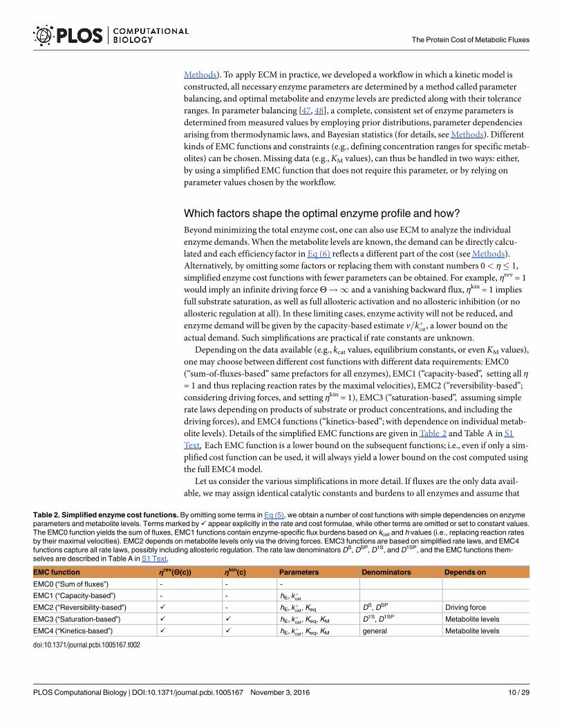
Table 2. Simplified enzyme cost functions. By omitting some terms in Eq (5), we obtain a number of cost functions with simple dependencies on enzyme

parameters and metabolite levels. Terms marked by ✓ appear explicitly in the rate and cost formulae, while other terms are omitted or set to constant values.

The EMC0 function yields the sum of fluxes, EMC1 functions contain enzyme-specific flux burdens based on kcat and h values (i.e., replacing reaction rates

by their maximal velocities). EMC2 depends on metabolite levels only via the driving forces. EMC3 functions are based on simplified rate laws, and EMC4

functions capture all rate laws, possibly including allosteric regulation. The rate law denominators DS, DSP, D1S, and D1SP, and the EMC functions them-

selves are described in Table A in S1 Text.

EMC function ηrev(Θ(c)) ηkin(c) Parameters Denominators Depends on

EMC0 (“Sum of fluxes”) - - -

EMC1 (“Capacity-based”) - - hE, kþcat

EMC2 (“Reversibility-based”) ✓ - hE, kþcat, Keq DS, DSP Driving force

EMC3 (“Saturation-based”) ✓ ✓ hE, kþcat, Keq, KM D1S, D1SP Metabolite levels

EMC4 (“Kinetics-based”) ✓ ✓ hE, kþcat, Keq, KM general Metabolite levels

doi:10.1371/journal.pcbi.1005167.t002



all reactions run at their maximal velocities. Then, enzyme levels and fluxes will be propor-tional for all reactions, the cost function in Eq (6) will be EMC0, and the cost will be propor-tional to the sum of fluxes. However, catalytic constants span many orders of magnitude [25],as do molecularmasses of enzymes, suggesting that EMC0 is an oversimplification. If individ-ual kþcat and hEl

values are known, we can define an individual flux burden acatvl¼ hEl

=kþcat l foreach enzyme, independent of metabolite levels. Then we obtain an EMC1 cost functionP

l acatvlvl, which is the same as the cost weights used in FBA with flux minimization [17] or

molecular crowding [19]. When kcat values are unknown, they can be estimated [42], replacedby “typical” values [25], or bounded by the value k1cat ¼ 108 1/s for a very fast, but diffusion-limited enzyme. The enzyme burdens hE can include factors like protein size, protein lifetime,covalent modifications, or space restrictions (see [20] and S1 Text section 2.1).

However, by assuming that enzymes work at their maximal rate and setting ηrev = ηkin = 1,we may obtain unrealistic results. First, the simplifying assumption ηrev = ηkin = 1 implies uncon-trollable metabolic states. In a kineticmodel with completely irreversible and substrate-saturatedenzymes, the reaction rates would be independent of metabolite levels and the steady-state fluxesand metabolite levels would depend on finely tuned enzyme levels [15]. Random variation inenzyme levels would lead to non-steady states, with fast accumulation or depletion of intermedi-ate metabolites. Such states are extremely fragile and thus uncontrollable. When assuming effi-ciencies ηrev or ηkin smaller than 1, we accept an increased cost and thereby acknowledge thatcontrol must be paid for by enzyme investments. Second, EMC1 functions underestimate allenzyme costs, and for reactions close to chemical equilibrium the errors may be quite large. Fora reactionGibbs energy of ΔrG0 = −0.1RT, the efficiencyof the catalyzing enzyme is reduced by afactor of ηrev = 1 − e0.1� 0.1, and the demand for enzyme increases by a factor of 1/ηrev� 10. Toaccount for this decreased efficiency, we can use EMC2 functions, which include the reversibilityfactor Zrev

l ¼ 1 � e� YlðxÞ. The driving forces are expressed in terms of metabolite log-concentra-tionsΘl(x) and equilibrium constants, which need to be known. This factor approaches infinityas reactions reach equilibrium (i.e. whereΘl! 0), which is what forces reactions away fromequilibriumduring cost minimization (see, for example, Fig 2).

The advantage of reversibility-based cost functions (EMC2) is that they are based on kcat

and equilibrium constants only. Several in-silicomethods exist to estimate Keq for virtually anybiochemical reaction [41, 49] and the values can be easily obtained at http://equilibrator.weizmann.ac.il/ [50]. As in the case of EMC1, kcat values can be estimated or set to a defaultconstant value. Methods like MDF [15] and mTOW [23] have been developed to addressexactly this situation, where detailed kinetic information is hard to obtain. We discuss the rela-tion between EMC2 and MDF in section 4 of the S1 Text. Aside from the EMC2 function,there are other reversibility-based estimates of the enzyme cost. For instance, the enzymedemand in Fig 2 (an EMC3-functionwith kinetic constants, fluxes, and enzyme burdens set to1) has the reversibility-based cost apw

v ¼P

l½1 � e� YðcÞ�� 1 as a lower bound. Since 1 − e−x� x

for all positive x, an even lower estimate is ∑lΘ(c)−1 (Figure B and Figure C in S1 Text). Somevariants of FBA relate fluxes to metabolite profiles, which are then required to be thermody-namically feasible, i.e., within the metabolite polytope. ECM constrains the metabolite profileseven further: as shown in Fig 2, profiles close to an E-face are very costly and can never be opti-mal. This holds for EMC2 functions and for the more realistic enzyme costs, which will even behigher. Thus, regions close to E-faces can be excluded from the polytope. At P-faces, defined byphysiological bounds, there will be no such increase, so the optimum may lie on a P-face (seeFig 2f). To exclude regions near E-faces, we simply define lower bounds for all driving forces(see S1 Text section 7.1). These bounds can be used both in ECM or in thermodynamic FBA toreduce the search space.



http://equilibrator.weizmann.ac.il/

http://equilibrator.weizmann.ac.il/

The next logical step is to relax the assumption that ηkin = 1. Just like the reversibility factorηrev, the kinetic factors ηsat and ηreg can be used to define tighter constraints on metabolite lev-els. However, unlike ηrev, the kinetic terms may take various forms and contain many kineticparameters. To obtain simple, but reasonable formulae in EMC3, we first consider rate laws inwhich enzyme molecules exist only in three possible states: unbound, bound to all substratemolecules, or bound to all product molecules.Metabolites affect the rate only through themass-action terms S = ∏i(si/KMi) (for substrates) and P = ∏j pi/KMj (for products), and thedegree of saturation is determined by ηsat = S/(1 + S + P), where the formula effectively has twoMichaelis-Menten constants: one for substrates and one for products (which are equivalent tothe product of all KMi and all KMj values). EMC3 represents a balance between complexity andrequirement for kinetic parameters, and is a practical cost function if simple, realistic rate lawsare desired. The EMC4 functions, finally, represent general rate laws and ηkin can take manydifferent forms depending on mechanism and order of enzyme-substrate binding. Again, forsimplicity, we resort to analyzing only a small set of relatively general templates for EMC4,known as convenience kinetics [51] or modular rate laws [21]. Nevertheless, our formalismallows a much wider range of rate laws, and we consider EMC4 a wild-card cost function thatcovers almost any reasonable rate law (see S1 Text section 2.2 for more details).

Enzyme and metabolite levels in E. coli central metabolism

To benchmark our optimality-based prediction of metabolite, we applied ECM to a model ofE. coli central metabolism, containing three major pathways: glycolysis, the pentose phos-phate pathway, and the TCA cycle (see Fig 3a, and Methods for modeling details). Fig 3b–3dcompares predicted enzyme profiles to measured protein levels [53]. The absolute values ofpredicted enzyme levels arise directly from the model, using the fluxes reported in [52],while cellular protein concentrations were obtained from proteomics data (measured insimilar conditions [53]) and assuming an average cell volume of * 1 fL (10−15 liters) [54].EMC4 predicts values that are of the right order of magnitude and reflect differences inenzyme levels along the pathways. The prediction error of 0.42 for enzyme levels (RMSE:root mean square error on a log10-scale) corresponds to a typical fold error of 10RMSE = 2.6.In line with the measured protein levels, the predicted enzyme levels tend to be larger in gly-colysis than in TCA and pentose phosphate pathway, reflecting the larger fluxes and less-favorable thermodynamics. All predictions including metabolite concentrations, thermody-namic forces and c/KM ratios can be found online at the accompanying website www.metabolic-economics.de/enzyme-cost-minimization/.

We note that predicted enzyme levels becomemore accurate as more complex cost func-tions are used, with a prediction error decreasingmonotonically from 1.35 with EMC0 to 0.42with EMC4. The capacity-based enzyme cost (EMC1) assumes that enzymes operate at fullcapacity (v ¼ E kþcat) and therefore underestimates all enzyme levels (Fig 3b). In reality, manyreactions in central metabolism are reversible and many substrates do not reach saturatingconcentrations. When taking these effects into account, predictions come closer to measuredenzyme levels (Fig 3c–3e). For instance, FUM (fumarase, fumA) and MDH (malate dehydroge-nase) have a much higher predicted level in EMC2-4 than in EMC1 as the reversibility-basedcosts account for their low driving forces. Similarly, the predicted levels of two pentose-phos-phate enzymes (ribulose-5-phosphate epimerase RPE and ribose phosphate isomerase RPI) aremuch higher in EMC3 and EMC4 because of their low affinity for the substrate ribulose-5-phosphate (Ru5P). In some cases, however, the more complex EMC4 fails to improve theprediction over the simpler methods. For instance, the 6-phosphogluconolactonase (PGL) andphosphoglycerate kinase (PGK) reactions are underestimated by all EMC functions, perhaps





due to regulation mechanisms that reduce activity such as allosteric inhibition. In very fewcases, EMC4 overestimates the level of an enzyme that has a more precise prediction in EMC1-3, e.g. phosphofructokinase (PFK). Overall, the EMC4 function performs substantially betteron average than the simpler cost functions even though it relies on a larger set of parameters,many of which are known with low certainty. Moreover, EMC4 predicts well the total of allenzyme levels (0.64 mM, compared to the measured value—0.62 mM), while the other EMCfunction underestimate this value (0.17, 0.24 and 0.43 mM for EMC1, EMC2 and EMC3respectively). To test the sensitivity of our results to the choice of parameters, we performedrandom sampling of kinetic constants, fluxes and fixed metabolite levels, and analyzed theeffect on the enzyme level predictions (see Methods and Fig 4a). We further tested the sensitiv-ity to our choice of proteomic data, by repeating the entire analysis using measured enzymeconcentrations from [55] and reached essentially the same findings (see Figure F in S1 Text).

Finally, we tested whether our kineticmodel can also predict enzyme levels without theassumption of cost optimality: to do so, we randomly sampled feasible metabolite profiles fromthe metabolite polytope, computed the resulting enzyme profiles, and compared them to prote-omic data. It turned out that the cost-optimal metabolite profile, or similar profiles, yielded sig-nificantly better predictions than metabolite profiles sampled from a broader range (see

Fig 3. Predicted enzyme levels in E. coli central metabolism. (a) Network model with pathways marked by colors. Flux magnitudes are represented

by the arrows’ thickness. (b) The ratio flux/kþcat (EMC1) as a predictor for enzyme levels. Points on the dashed line would represent precise predictions. (c)

Enzyme levels predicted by the reversibility-based EMC2(S) function. Vertical bars indicate tolerance ranges obtained from a relaxed optimality condition

(allowing for a one percent increase in total enzyme cost). (d) Enzyme levels predicted with EMC3 function representing fast substrate or product

binding. (e) Enzyme levels predicted with EMC4 function based on the common modular rate law [21]. In all sub-figures (b-e), RMSE is the root mean

squared error (in log10-scale) of our predictions compared to the measured enzyme levels, and r stands for the Pearson correlation coefficient.

Predictions are based on fluxes from [52], kþcat and KM values from BRENDA [40], and compared to protein data from [53]. For metabolite predictions, see

Figure E in S1 Text.




Methods and Fig 4b). This supports the hypothesis that cost-optimality shapes the metabolicstate in E. coli.

Although ECM puts enzymes on a pedestal due to their relatively high cost, the metaboliteconcentrations are key to minimizing that cost. One would thus expect to find good correspon-dence between the predicted metabolite profile and concentrations measured in vivo, especiallywhen predictions of enzyme levels are good. Since some EMC functions leave metabolite levelsunderdetermined,we penalized very high or low metabolite concentrations by adding a second,concentration-dependent objective to the optimization problem. In particular for EMC0 andEMC1, this regularization term is the only term—aside from global constraints—that deter-mines the metabolite concentrations as they do not affect enzyme cost whatsoever. In all othercases, the term mostly influencesmetabolites that have a minimal effect on the cost. Compar-ing the EMC metabolite prediction with in-vivo experimental data, as shown in Figure E in S1Text, the predicted metabolite levels are in the correct scale. Similar to enzyme level predic-tions, EMC4cm has the smallest prediction error—about 0.62 (corresponding to a typical folderror of 4.1).

We can now use EMC analysis to rationalize cellular enzyme levels. Fig 5 (like the scheme inFig 1b) shows the specific contributions to enzyme demand for each reaction. The reversibilitycost terms provided by EMC2s (purple bars in Fig 5a) improve the enzyme demand predictionsin most cases, compared to the basic capacity-based costs. However, the EMC4cm predictionsshow that saturation-based costs (orange bars in Fig 5b) are often larger than the reversibilitycosts, and they improve the predictions even more. For practical cost estimates, for examplewhen computing flux burdens for FBA, we can conclude that multiplying the experimentally

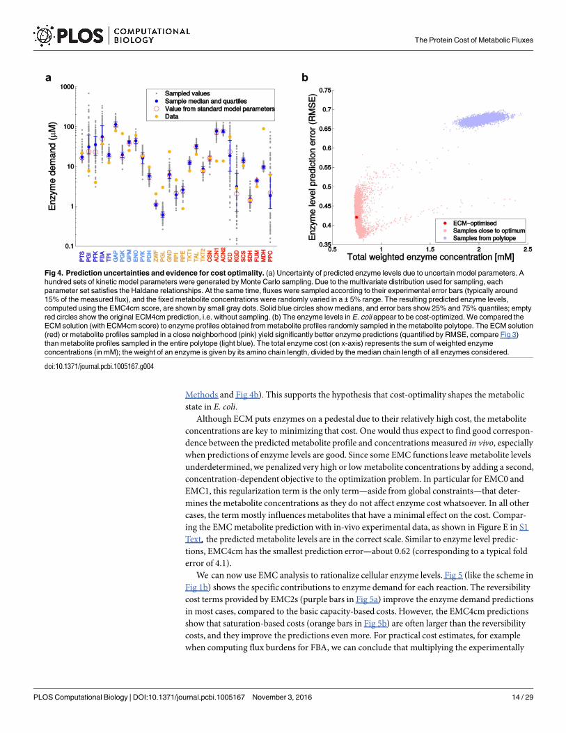
Fig 4. Prediction uncertainties and evidence for cost optimality. (a) Uncertainty of predicted enzyme levels due to uncertain model parameters. A

hundred sets of kinetic model parameters were generated by Monte Carlo sampling. Due to the multivariate distribution used for sampling, each

parameter set satisfies the Haldane relationships. At the same time, fluxes were sampled according to their experimental error bars (typically around

15% of the measured flux), and the fixed metabolite concentrations were randomly varied in a ± 5% range. The resulting predicted enzyme levels,

computed using the EMC4cm score, are shown by small gray dots. Solid blue circles show medians, and error bars show 25% and 75% quantiles; empty

red circles show the original ECM4cm prediction, i.e. without sampling. (b) The enzyme levels in E. coli appear to be cost-optimized. We compared the

ECM solution (with ECM4cm score) to enzyme profiles obtained from metabolite profiles randomly sampled in the metabolite polytope. The ECM solution

(red) or metabolite profiles sampled in a close neighborhood (pink) yield significantly better enzyme predictions (quantified by RMSE, compare Fig 3)

than metabolite profiles sampled in the entire polytope (light blue). The total enzyme cost (on x-axis) represents the sum of weighted enzyme

concentrations (in mM); the weight of an enzyme is given by its amino chain length, divided by the median chain length of all enzymes considered.




determined kcat values by reversibility factors will likely improve the fidelity of FBA predic-tions. For more details, see S1 Text section 4.

Discussion

When applying mathematical models to learn about biology, one typically faces a conflictbetweenmodel accuracy and the amount of available data. Metabolic systems are known toabide to several physical and physiological considerations, all of which are mathematicallywell-described (e.g. flux balance, thermodynamics, kinetics, and cost-benefit optimality). Tak-ing all of these aspects into account would create very detailedmodels but at the price of con-siderably increasing the demand for data. Here, we obtained a flexible modelingmethod bycombining the two main modeling approaches, constraint-based and kineticmodeling, in anew way: with fixed metabolic fluxes, kineticmodels are used to determine a cost-optimalstate. The tiered approach in ECM allows for different levels of detail, which can easily bematched to the amount of existing data. The minimal requirement for running ECM is to havea metabolic network with given steady-state fluxes, while the maximal requirement would be afully parameterized kinetic model. The method applies to individual metabolic pathways and,theoretically, entire metabolic networks. No matter if we model exponentially growing cells,microbial cells in stationary phase, or non-growing eukaryotic cells, the sum of enzyme costsper unit flux is a meaningful objective for pathways used by the cell. Although similarapproaches exist in dynamic modeling [48, 56] and enzyme optimization [4, 15, 23], ECMextends these ideas to the most general kinetic rate laws and cost functions, while proving thatthe emerging optimization problem is convex and thus easily (albeit numerically) solvable.ECM advances metabolic modeling in six different ways:

Fig 5. Enzyme demand in central metabolism. (a) Measured fluxes for all reactions (black dots on top) lead to an enzyme demand (bottom). The

enzyme demand, predicted by using the reversibility-based EMC2s cost function, can be split into factors representing enzyme capacity and

thermodynamics (see Methods). Bars show predicted enzyme levels in mM for individual enzymes on logarithmic scale. Yellow dots denote measured

enzyme levels (in μM). Note that the bars do not represent additive costs, but multiplicative cost terms on logarithmic scale; therefore, the relevant

feature of the blue bars is not their absolute lengths, but their differences between enzymes. (b) The kinetics-based EMC4cm cost function includes

saturation terms and yields more accurate predictions. Starting from the capacity cost (in blue), the reversibility (purple) and saturation (red) terms

increase the enzyme demands and decrease the variability between enzymes (on log-scale). Note that flux data (circles) and protein data (yellow dots)

are identical in both plots.




1. Solving the enzyme optimality problem in metabolite spaceOne way of modeling thecost and benefit of enzymes is to study kineticmodels and to treat enzyme levels as free vari-ables to be optimized. However, this calculation can be hard because enzyme profiles may leadto one, several, or no steady states, and the resulting optimality problem can be non-convex. Byfixing fluxes and using metabolite concentrations as our primary variables, we drastically sim-plify this optimization problem. Flux directions and the second law of thermodynamics imposeconstraints that define a set of feasible metabolite profiles, the metabolite polytope. This poly-tope is used here as a space for screening, sampling, and optimizing metabolic states; accord-ingly bounds on metabolite concentrations or driving forces can be easily formulated as linearconstraints. Using log-concentrations as free variables, and given a (steady and non-steady)flux distribution, we can parametrize the set of metabolic states very easily: we simply considerall feasible metabolite profiles and compute, for each of them, the corresponding enzyme pro-file by taking the inverse rate laws. With enzyme levels as free variables, parameterizing the setof metabolic states would be much more complicated.

2. Convexity The metabolite polytope not only provides a good search space, but it alsofacilitates optimization because enzyme cost is a convex function of the metabolite log-concen-trations (see S1 Text section 3.2). Convexity makes the optimization tractable and scalable—unlike a direct optimization in enzyme space. Simple convexity holds for a wide range of ratelaws and for extended versions of the problem, e.g., including bounds on the sum of (non-loga-rithmic) metabolite levels or bounds on weighted sums of enzyme fractions. By using specificrate laws (e.g., the ECM4cm rate law, as shown by our colleague Joost Hulshof—personal com-munication) or by adding a regularization term, representing additional biological objectives,we can even ensure strict convexity, and thus the existence of a unique optimum that can beefficiently found. It is important to distinguish this computational scalability, which is facili-tated by convexity, from other pragmatic issues that arise when increasing the scale of a model,in particular the scarcity of kinetic data. Standard kinetic modeling is difficult to apply towhole-cell metabolic networks due to both scalability problems. Therefore, even if network-wide kcat and KM values were to become available (e.g. by estimation methods that rely onhigh-throughput data [42]), it would still be impractical to exhaustively search the parameterspace. ECM—due to its convexity—is solvable even on a genomic scale.

3. Separable rate laws disentangle individual enzyme cost effectsTo assess how differentphysical factors shape metabolic states, we focused on separable rate laws, which lead to a seriesof easily interpretable, convex cost functions. The terms in these functions represent specificphysical factors and require different kinetic and thermodynamic data for their calculation. Byneglecting some of the terms, one obtains different approximations of the true enzyme cost.The more terms are considered, the more precise our predictions about metabolic statesbecomes (see Methods and S1 Text section 2). By comparing the different scores, we can esti-mate the enzyme cost that cells “pay” for running reactions at small driving forces (to saveGibbs free energy) or for keeping enzymes beneath substrate-saturation (e.g., to dampen fluc-tuations in metabolite levels). Of course, it is often important to keep models simple and thenumber of parameters small, and therefore the stripped-down versions of ECM can be usefulin practice. For example, in some conditions such as batch-fed E. coli, a simple enzyme econ-omy might still be a realistic approximation. Our results in Fig 3 indicate that indeed one canpredict enzyme levels quite well even with relatively simple enzyme cost objectives. Finally, inconditions where ECM’s predictions are far from the measured enzyme levels, we can focus onspecific enzymes or pathways that deviate the most, which may therefore display optimizationor adaptations beyond simple resource allocation.

4. Relationship to other optimality approaches Beyond the practical advantages of usingfactorized enzyme cost functions, they also allow us to easily compare our methods to earlier



approaches. These approaches typically focused on only one or two of the factors that are takeninto account in ECM, and many of them can be reformulated as approximations of ECM (aswe have shown for MDF [15] and, by proxy, earlier thermodynamic profiling methods [57,58]). For example, the optimization performed by FBA with flux minimization is equivalent tousing EMC0, while EMC1 is based on the same principles as FBA with molecular crowding[19], pathway specific activities [2], and ConstrainedAllocation Flux Balance Analysis(CAFBA) [59]. Thermodynamic profiling methods [15, 57, 58] which use driving forces as aproxy for the cost, can be compared to EMC2 (where all kcat are assumed to be equal, see S1Text section 4). To our knowledge, ECM is the first method that accounts for substrate andproduct saturation (as well as allosteric) effects in the optimization process and guarantees aconvex (i.e., relatively tractable) optimality problem. Moreover, ECM highlights how differentaspects of metabolism are linked: most importantly, thermodynamic feasibility [15] is general-ized by the quantitative notion of thermodynamic efficiency, which then turns out to be a natu-ral precondition for enzyme economy.

5. Kinetics-basedflux cost functions for flux balance analysisAccordingly, results fromECM can be used to improve flux analysis [13, 23] by definingmore realistic flux cost functionsfor FBA and by providing formulae for the pathway specific activity [2] (see S1 Text section2.3). In practice, the cost weights used in FBA so far (typically, defined by kcat values and enzymesizes) could be adjusted by dividing them by efficiency factors obtained from our workflow. InFBA (specifically in variants with flux minimization or molecular crowding), flux cost orenzyme demand are linear functions of the fluxes. Enzyme Cost Minimization allows us to com-pute plausible prefactors for this formula from detailed knowledge of enzyme kinetics: by rear-ranging Eq (6), we can write the enzyme cost as a linear function q ¼

X

lavl � vl with flux

burdens avlðcÞ ¼ hEl� 1

kþcat;l� 1

Zrevl ðcÞ� 1

Zsatl ðcÞ� 1

ZregðcÞ. The flux burden has a lower bound acatvl¼ hEl

=kþcat;l,

denoting the cost per flux under ideal conditions. Ignoring all dependencies on metabolite levels,acatvl

could be used as a cost weight to define flux cost functions for FBA. However, these valuesare further increased by the reciprocal values of the enzyme efficiency factors. A similar, flux-specific enzyme cost (or, inversely, a flux per enzyme invested) can also be defined for entirepathways. The Pathway Specific Activity (PSA) [2] is defined as the flux per enzyme mass (inunits of mmol/s per mg of enzyme) and can be computed by treating enzyme mass as a costfunction.Assuming that ηrev = ηkin = 1 and that cost is expressed in terms of protein mass inDaltons ðhEl

¼ mlÞ, we obtain the pathway specific activity using the formula Apw = vpw/q.6. EmbeddingECM into flux analysis Furthermore, ECM could be “embedded” into FBA

by screening a finite set of possible flux distributions, characterizing each of them by quantita-tive cost (using ECM) and choosing the most cost-favorable mode. Since we now know thatany metabolic state that has maximal specific rate is an elementary flux mode [60], it would besufficient to scan only the elementary flux modes. This could be seen as a version of minimal-flux FBA, but one that uses kinetic knowledge instead of the various heuristic assumptions thatgo into FBA. Second, we can derive realistic bounds on thermodynamic forces based on kinet-ics and enzyme cost, or lower/upper bounds on substrates/products concentrations to avoidextreme saturation effects. All these constraints follow systematically from setting upper limitson the individual efficiency factors. By applying them in thermodynamics-based flux analysis,we shrink the metabolite polytope by excluding strips at its boundarywhere costs would be toohigh to allow for an optimal state. Similarly, by giving individual weights to thermodynamicdriving forces, MDF could be used as a method to optimize some lower bound on the system’senzyme cost (see S1 Text section 4).

ECM is based on the central assumptions that the metabolic states of cells are cost-opti-mized and that cost arises from cellular protein levels. Both assumptions are of course



debatable. There is ample evidence that cells assume apparently sub-optimal states in order tomaintain robust homeostasis or to gain metabolic flexibility for addressing future challenges[1]. For example, an allosterically regulated enzyme will often not reach its maximal possibleactivity, so investment in enzyme production appears to be wasted. Nevertheless, cells pay thisprice in order to gain the ability to adjust quickly to changes (i.e. within seconds rather thanthe minutes required for altering gene expression). One intriguing example is the bacteriumLactococcus lactis, which uses the exact same enzyme expression profile for completely differ-ent anaerobic growth modes [61]: slow growth / high yield acetate fermentation, and fastgrowth / low yield lactate fermentation. The reason that low-yield strategies achieve highergrowth rates is typically attributed to much lower protein investments, but obviously, this isnot the case in the Lactococcus lactis experiments. This stands in contrast to aerobic fermenta-tion in E. coli, which seems to be explained well by predictable shifts in protein allocation [5].

As these examples show us, the importance that certain cells attribute to saving on proteincosts is highly variable and, in some cases, can be negligible: for instance, when protein levelsare already low or when protein demands change quickly and unpredictably. Moreover, ran-dom fluctuations in protein levels will be tolerable as long as the impact on fitness is not veryhigh. Nevertheless, we think that a simple principle of cost optimality as in ECM can be a usefulheuristics. On the one hand, it can reveal theminimal protein investment that would berequired to support a certainmetabolic state. In metabolic engineering, such predicted invest-ments may be used to rule out potential, but uneconomicalmetabolic pathways. On the otherhand, ECM can be used as a background model to be compared to more complicated optimal-ity-based cell models. Such comparisons can allow us to quantify the impact of other fitnessobjectives in units of “protein cost”, to learn which objectives can best explain cellular behavior,and to describe non-optimality as a deviation from a presumable cost-optimal state.

Furthermore, ECM can be extended to cover more realistic optimality scenarios. Some alter-native objectives can be integrated into ECM by adding them to the objective function.Wehave tried to keep our method as general as possible to facilitate such objectives, e.g. by allow-ing for non-linear, convex enzyme costs (h(E)). In particular, metabolite levels may be underadditional constraints or optimality pressures because they appear in pathways outside ourmodel, which may favor high or low levels of the metabolites. Also chemical molecule proper-ties, such as hydrophobicity or charge, may affect the preferable metabolite levels in cells [62].For example, if our model captures an ATP-producing pathway, low ATP levels will be ener-getically favorable, whereas other ATP-consuming pathways would favor higher ATP levels.To account for this trade-off, a requirement for sufficiently high ATP levels can be included inour ECM model by constraints or additional objectives b(c)(x) that penalize low ATP levels (seeMethods). If metabolite levels are kept far from their upper or lower physiological bounds, thiswill allow for more flexible adjustments in case of perturbation.

If enzyme profiles were shaped by optimal resource allocation, as assumed in ECM, thiswould have consequences for the shapes of enzyme and metabolite profiles. Enzyme cost, ther-modynamic forces, and an avoidance of low substrate levels would be tightly entangled, andthe shapes of enzyme profiles would reflect the role of enzymes in metabolism, i.e., the way inwhich they control metabolic concentrations and fluxes. Among other things, this would implythree general properties of enzyme profiles:

1. Enzyme cost is related to thermodynamics In FBA, thermodynamic constraints andflux costs appear as completely unrelated aspects of metabolism. Thermodynamics is used torestrict flux directions, and to relate them to metabolite bounds, while flux costs are used tosuppress unnecessary fluxes. In ECM, thermodynamics and flux cost appear as two sides of acoin. Like in FBA, flux profiles are thermodynamically feasible if they lead to a finite-sizedmetabolite polytope, allowing for positive forces in all reactions. However, the values of these



forces also play a role in shaping the enzyme cost function on that polytope. Together, metabo-lite polytope and enzyme cost function (as in Fig 2) summarize all relevant information aboutflux cost.

2. Enzymeprofiles reflect localmetabolic necessitiesWhat are the factors that determinethe levels of specific enzymes? High levels are required whenever catalytic constants, drivingforces, or substrate concentrations are low. Accordingly, an efficient use of enzymes requiresmetabolite profiles with sufficient driving forces (for energetic efficiency) and sufficient sub-strate levels (for saturation efficiency).Trade-offs between these requirements, together withpredefined bounds, will shape the optimal metabolite profiles [23]: in a linear pathway, a needfor energetic efficiencywill push substrate concentrations up and product concentrationsdown; the need for saturation efficiencyhas the same effect. However, since the product of onereaction is the substrate of another reaction, there will be trade-offs between efficiencies in dif-ferent reactions. Therefore, where enzymes are costly or show low kcat values, we may expect astrong pressure on sufficient driving forces and substrate levels.

3. Enzymeprofiles reflect global effects of enzyme usage If enzyme profiles follow a cost-benefit principle, costly enzymes should provide large benefits. Such a correspondence hasbeen predicted, for example, from kineticmodels in which flux is maximized at a fixed totalenzyme investment [63]: in optimal states, high-abundance enzymes exert a strong control onthe flux, and enzymes with strong flux control are highly abundant. If this applies in reality,then high investment (e.g., large enzyme levels shown in Fig 1A) could be seen as a sign oflarge benefit, in terms of flux control. Here, we studied a different optimality problem (fixingthe fluxes and optimizing enzyme levels under constraints on metabolite levels), and obtain amore general result. The optimal enzyme cost profile obtained by ECM is a linear combinationof flux control coefficients and, possibly, control coefficients on metabolites that hit upper orlower bounds (see S1 Text section 7.4). In simple cases (e.g., the example in Fig 2), where thereis only one flux mode and none of the metabolites hits a bound, enzyme demands and flux con-trol coefficientswill be directly proportional.

Beyond the analysis of central metabolism, ECM can be applied to select candidate path-ways in metabolic engineering projects. A prediction of enzyme demands or specific activities(S1 Text section 2.3) can be helpful at different stages of pathway design. The optimal expres-sion profile for a pathway can be determined, critical steps in a pathway can be detected (i.e.,steps where lowering the enzyme’s flux-specific cost avl would be most important), and enzymedemand and cost can be compared between pathway structures. This type of application is notunique to ECM, and although several of the methods that we mention throughout this manu-script [2, 4, 23, 32, 64, 65] have been used for this purpose in the past, we believe that ECMmanages to bring them all under one umbrella.

Materials and Methods

Metabolite polytope and enzyme cost functions

A metabolic network with given flux directions, equilibrium constants, and metabolite boundsdefines themetabolite polytope. This convex polytope P in the space of log-concentrations xi =ln ci represents the set of feasible metabolite profiles. The flux profile used can be stationary(e.g. determined by FBA or 13C MFA) or non-stationary (e.g. from dynamic 13C labeling exper-iments [66]). If the provided flux directions are thermodynamically infeasible, the metabolitepolytope will be an empty set, P ¼ ;. The faces of the metabolite polytope arise from twotypes of inequality constraints. First, the physical ranges xmin

i � xi � xmaxi of metabolite levels

define a box-shaped polytope (bounded by P-faces). Some metabolite levels may even be con-strained to fixed values. Second, each reaction must dissipate Gibbs free energy, and to make



this possible, driving forces and fluxes must have the same signs (Θl � vl> 0), andthus signðvlÞ ¼ signðDrG0

�

l =RT þP

inilxiÞ. The resulting constraints define E-faces of themetabolite polytope (representing equilibrium states, Θl = 0). Close to these faces, enzyme costgoes to infinity.

Separable rate laws and enzyme cost functions

According to Eq (3), reversible rate laws can be factorized into four terms: the enzyme level E,its forward catalytic constants kþcat, and two efficiency factors [22]. In Fig 6 we add a non-com-petitive allosteric inhibitor x. While the enzyme level and kþcat are not directly affected by theconcentration of metabolites (although kþcat can vary with conditions such as pH, ionic strength,or molecular crowding in cells), the efficiency factors are concentration-dependent, unitless,and can vary between 0 and 1. The reversibility factor ηrev depends on the driving force (andthus, indirectly, on metabolite levels), and the equilibrium constant is required for its calcula-tion. The saturation factor ηsat depends directly on metabolite levels and contains theKM valuesas parameters. Allosteric regulation yields additive or multiplicative terms in the rate lawdenominator, which in our example can be captured by a separate factor ηreg. In general, ηsat

and ηreg can be combined into one kinetic factor ηkin, as depicted in Eq 6.The second equation in Fig 6 describes the enzyme cost for a flux v, and contains the terms

from the rate law in inverse form multiplied by the enzyme burden hE. The left-hand part of theequation, hE v=kþcat, defines a minimum enzyme cost, which is then increased by the followingefficiency factors. Again, 1/ηkin can be split into 1/ηsat � 1/ηreg. By omitting some of these factors,one can construct simplified enzyme cost functions with higher specific rates, or lower enzymedemands (compare Fig 1b). Since both rate and enzyme demand are a product of several terms,

Fig 6. Rate law and enzyme demand of reversible Meichalis-Menten reactions. For a reaction SÐ P

with reversible Michaelis-Menten kinetics, a driving force θ = −ΔrG0/RT, and a prefactor for non-competitive

allosteric inhibition, the rate law can be written as with inhibitor concentration x. In the example, with non-

competitive allosteric inhibition, the kinetic factor ηkin could even be split into a product ηsat � ηreg. The first two

terms in our example, E � kþcat, represent the maximal velocity (the rate at full substrate-saturation, no

backward flux, full allosteric activation), while the following factors decrease this velocity for different

reasons: the factor ηrev describes a decrease due to backward fluxes (see Figure A in S1 Text) and the factor

ηkin describes a further decrease due to incomplete substrate saturation and allosteric regulation (see Fig

1b). The inverse of all these terms appear in the equation for enzyme demand, q, which is given by the

enzyme level multiplied by the burden of that enzyme, hE.




it is convenient to depict them as a sum on a logarithmic scale (Fig 7), where the simplified func-tions are seen as upper/lower bounds on the more complex rate/demand functions.

Enzyme cost minimization can be formulated as a convex optimality

problem for metabolite levels

Enzyme cost minimization (ECM) uses a metabolic network, a flux profile v, kinetic rate laws,enzyme burdens, and bounds on metabolite levels to predict optimal metabolite and enzymeconcentrations. The enzyme cost of reactions or pathways is a convex function on the metabo-lite polytope (proof in S1 Text section 3.2), that is, a log-scalemetabolite vector x, linearly inter-polated between vectors xa and xb, cannot have a higher cost than the interpolated cost of xa

and xb. Convexity also holds for cost functions h(E) that are non-linear, but convex over E.Some EMC functions are strictly convex (i.e., Eq. (S18) holds with a< sign instead of�), whileothers are not (e.g. EMC2). The most simplified EMC functions are actually constant (as inEMC0 and EMC1). To find an optimal state, we choose an EMC function and minimize thetotal enzyme cost within the metabolite polytope. Optimal metabolite profiles, enzyme profiles,and enzyme costs are obtained by solving the enzyme cost minimization (ECM) problem

xoptðvÞ ¼ argminx2P qðx;vÞ

EoptðvÞ ¼ EðxoptðvÞ;vÞ

qoptðvÞ ¼ qðxopt;vÞ:

ð7Þ

The total cost q(x, v) (defined in Eq (6)) is the sum of enzyme costs given by EMC functions.Since q(x) and the metabolite polytope itself are convex, ECM is a convex optimization problem.The optimal enzyme levels depend on external conditions and have to be recalculated after anychange in external metabolite levels. There are cases where q(x) is convex, but not strictly con-vex, and therefore Eq (7) will have a continuum of optimal metabolite solutions. This holds, inparticular, for EMC1 scores, which are independent of metabolite levels, and for EMC2 scores,which only depend on reaction Gibbs free energies, i.e., on some linear combinations of the log-arithmic metabolite levels. In such cases, to enforce a unique solution one may add a strictly

Fig 7. The conversion between fluxes and enzyme levels, in both directions. (a) Starting from the

logarithmic enzyme level (dashed line on top), we add the terms log kþcat, log ηrev, and log ηkin, and obtain

better and better approximation of the rate. In the example shown, kþcat has a numerical value smaller than 1.

The more precise approximations (with more terms) yield smaller rates. The EMC4 arrows refer to other

possible rate laws with additional terms in the denominator. (b) Enzyme demand is shaped by the same

factors (see Eq (5)). Starting from a desired flux (bottom line), the predicted demand increases as more

terms are considered.




convex side objective that scores the log-metabolite levels, e.g., a quadratic function favoringmetabolite levels close to some typical concentration vector x : minx2P ðqðx; vÞ þ ljjx � xjjÞ,where λ is a small, heuristically chosen weighing factor (see S1 Text section 3.3). Such extraobjectives can be justified biologically, e.g. by assuming that intermediate metabolite levels givecells more flexibility to adapt to perturbations. Strict convexity not only simplifies numerical cal-culations, but it also guarantees that the optimization problem has a unique solution. In fact,metabolite polytope and cost functions remain convex even under various modifications of theproblem. When adding constraints on the total metabolite level, on weighted sums of metabolitelevels, or on weighted sums of enzyme levels, the metabolite polytope is intersectedwith curvedmanifolds (since we are dealing with concentrations in logarithmic scale) but remains convex(S1 Text section 3.4). Finally, we can consider the more complicated problem of preemptiveenzyme expression, where a fixed enzyme profile and allosteric inhibition must allow a cell torealize different flux distributions under different conditions. Also this problem is convex (S1Text section 3.7). If a model contains non-enzymatic reactions (or non-enzymatic processessuch as metabolite diffusion out of the cell or dilution in growing cells), each such reaction leadsto an extra constraint on the metabolite polytope (S1 Text section 3.8). A known flux in an irre-versible diffusion or dilution reaction fixes the concentration of one metabolite. In the presenceof irreversible non-enzymatic reactions with mass-action rate laws, the polytope is intersectedby a subspace. In both cases, the resulting sub-polytope may be empty, i.e., the given flux distri-bution will not be realizable.

Non-stationary states and the importance of boundary metabolites

Flux balance analysis and kineticmodels rely on the assumption that certainmetabolites aremass-balanced: in FBA, this assumption, together with stationarity, defines the set of steady-state fluxes; in kineticmodels, the mass-balancedmetabolites are the ones whose dynamics isdescribedby the system equations. ECM, in contrast, assumes fluxes to be given and makes noassumption about mass balances. If the fluxes in our pathway model lead to a mass imbalance ina metabolite, we may still assume that the entire cell is in stationary state, but that mass balancesare reached with the help of other pathways that are not part of our model. Alternatively, wemay assume that the metabolite is actually not mass-balanced and that we are describing a non-stationary, transient state. In both cases, ECM is fully applicable as long as metabolic fluxes arepredefined and loop-less (in order to be realizable by a thermodynamically consistent state [67]).

A key point in ECM is the choice of metabolite levels on the model boundary. If we prede-fine all these metabolite levels, our pathway will be “isolated” from the rest of the network, andany information about the surrounding network can be safely ignored. In our E. coli model,ATP is one such important boundarymetabolite: if we allowed for a lower ATP level, ATPcould be produced at a lower enzyme cost because of the more favorable driving forces. If wedo not fix the ATP concentration, but define an allowed range, ECM would choose the lowestpossible ATP level; thus, if the allowed ATP range is too broad, no meaningful predictions canbe expected. In a model of ATP-consuming biosynthesis pathways, the situation would beexactly the opposite: here, it is a high ATP level that would lead to higher driving forces and tolower enzyme requirements. Whole-cell models contain both types of pathways—ATP-pro-ducing and ATP-consuming ones. In such a model, ECM could predict some meaningful com-promise, i.e. an intermediate ATP level that minimizes the enzyme cost of ATP productionplus the enzyme cost of biosynthesis. Since in our central metabolism model there are only 3reactions that produce or consume ATP, it is unlikely that so few reactions would be represen-tative of the cost tradeoff between the dozens of enzymes that use ATP in the full metabolicnetwork. Therefore, we chose to fix the ATP level to its measured value (*3 mM).



Our use of small-scale pathway models, which ignore most of the metabolic network, istherefore justified: as long as we predefine all metabolic fluxes and all metabolite levels at thepathway boundary, pathways can be modeled separately and the models can later be combinedwithout any adjustment. This makes the ECM approach fully modular. All the input parame-ters (kinetic parameters, fluxes and boundary concentrations) are directly obtained from mea-surements without any further tuning. By setting all relevant fluxes and boundarymetaboliteconcentrations to their measured values, we isolate our submodel from any effects that the sur-rounding network might have on predicted enzyme cost. Finally, there may be metabolites thatare “free” in a model, but that affect enzymes that are not in the model (e.g. pyruvate, whichaffects 30 other enzymes). By neglecting these enzymes, we ignore some of the complex com-promises between them, and the predicted metabolite concentration may be wrong. In our spe-cific case of central metabolism, whose enzymes comprise a very large fraction of E. coli’sproteome, this effect is probably not so severe. In any case, this problem can be easily fixed byimposing constraints or fixed concentrations for central metabolites such as pyruvate (similarto how we deal with ATP and other co-factors).

Tolerance ranges for nearly optimal solutions

Evolution could tolerate non-optimal enzyme costs; this tolerance depends on populationdynamics and can sometimes be quite significant, e.g. in small isolated communities. To com-pute realistic tolerance ranges for the ECM problem, we start from the optimum (total cost q)and choose a tolerable cost qtol (e.g., one percent higher than the optimal cost). This defines atolerable region in P : P tol � fx 2 P j qðxÞ � qtolg. A tolerance range for each metabolite isdefined by the minimal and maximal values the metabolite can show within Ptol. Toleranceranges for enzyme levels are defined in a similar way. Alternatively, tolerance ranges and nearlyoptimal solutions can be estimated from the Hessian matrix (see S1 Text section 7.3).

Sensitivity analysis with respect to kinetic constants

The predicted enzyme and metabolite levels depend on the kineticmodel chosen, and in partic-ular on the kinetic constants (kcat and KM values). Errors or uncertainties in these constantswill cause errors or uncertainties in the predicted enzyme profiles. To estimate these uncertain-ties, we considered a joint distribution of all model parameters, describing both the uncertain-ties of individual parameters and the correlations between dependent parameters. Thisprobability distribution was directly obtained from parameter balancing (S1 Text section 5.2).We sampled the kinetic parameters from this distribution, sampled metabolic fluxes accordingto their experimentalmean values and standard deviations, and varied the fixed metabolite lev-els in a ± 5% range around their standard values. Then we applied ECM on each of the sampledparameter sets, and gathered statistics for the optimal enzyme and metabolite levels. Fig 4(a)shows the distributions of the predicted enzyme levels. For narrow parameter distributions, themean values, variances, and covariances of the predicted enzyme levels can even be computed,approximately, from the ECM solution with standard parameters (see S1 Text section 3.5).Enzyme uncertainties caused by parameter uncertainties should not be confusedwith the toler-ance ranges describedbefore. The tolerance ranges are always associated with sub-optimalsolutions, i.e., enzyme profiles with a higher total cost; enzyme variations caused by parametervariation, in contrast, can go both ways and may sometimes decrease the cost.

Testing the hypothesis of cost-optimal metabolite profiles

Our enzyme level predictions rely on two main assumptions: a mechanistic model that definesa quantitative relation betweenmetabolite levels, enzyme levels, and fluxes, and an optimality



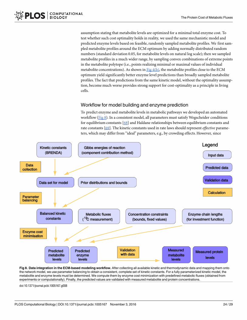
assumption stating that metabolite levels are optimized for a minimal total enzyme cost. Totest whether such cost optimality holds in reality, we used the same mechanistic model andpredicted enzyme levels based on feasible, randomly sampled metabolite profiles. We first sam-pled metabolite profiles around the ECM optimum by adding normally distributed randomnumbers (standard deviation 0.05, for metabolite levels on natural log scale); then we sampledmetabolite profiles in a much wider range, by sampling convex combinations of extreme pointsin the metabolite polytope (i.e., points realizing minimal or maximal values of individualmetabolite concentrations). As shown in Fig 4(b), the metabolite profiles close to the ECMoptimum yield significantly better enzyme level predictions than broadly sampled metaboliteprofiles. The fact that predictions from the same kineticmodel, without the optimality assump-tion, becomemuch worse provides strong support for cost-optimality as a principle in livingcells.

Workflow for model building and enzyme prediction

To predict enzyme and metabolite levels in metabolic pathways we developed an automatedworkflow (Fig 8). In a consistent model, all parameters must satisfy Wegscheider conditionsfor equilibrium constants [68] and Haldane relationships between equilibrium constants andrate constants [69]. The kinetic constants used in rate laws should represent effective parame-ters, which may differ from “ideal” parameters, e.g., by crowding effects. However, since

Fig 8. Data integration in the ECM-based modeling workflow. After collecting all available kinetic and thermodynamic data and mapping them onto

the network model, we use parameter balancing to obtain a consistent, complete set of kinetic constants. For a fully parameterized kinetic model, the

metabolite and enzyme levels must be determined. We compute them by enzyme cost minimization with predefined metabolic fluxes (obtained from

experiments or computationally). Finally, the predicted values are validated with measured metabolite and protein concentrations.




measured parameter values are usually incomplete and inconsistent, parameter balancing [47]is used to translate measured kinetic constants into consistent model parameters. Based on anetwork and given fluxes, the software extracts relevant data from a database (thermodynamicconstants, rate constants, fluxes, and protein sizes; metabolite and protein levels for validation),determines a consistent set of model parameters, builds a kineticmodel, and optimizes enzymeand metabolite profiles for the EMC function chosen. To assess the effects of parameter varia-tion, parameter sets can be sampled from the posterior distribution as described above. Theworkflow has been implemented in MATLAB and uses Systems BiologyMarkup Language(SBML) for model structures and the SBtab table format for numerical data [70].

E. coli model

The model shown in Fig 3 was built automatically from a list of chemical reactions in E. colicentral metabolism (for details, see S1 Text section 6). Equilibrium constants were estimatedusing the component contribution method [41], kinetic constants (kþcat and KM values) wereobtained from the BRENDA database (after which each value was curated manually), and acomplete, globally consistent parameter set was determined by parameter balancing. DuringECM, all metabolite levels were limited to predefined ranges, and the levels of cofactors andsome other metabolites were fixed at experimentally known values. To compute tolerances forpredicted metabolite and enzyme levels, we defined an acceptable enzyme cost, one percenthigher than the minimal value, and determined ranges for metabolite levels that agree with thiscost limit. The enzyme cost function accounts for protein composition, giving different costs todifferent amino acids. However, models with equal cost weights for all proteins, or with size-dependent protein costs yielded similar results (results are provided on the website). Data,model, and MATLAB code for ECM can be obtained from www.metabolic-economics.de/enzyme-cost-minimization/.

Supporting Information

S1 Text. Supplementarymaterial text containing Figure A—Figure F and Table A—Table C.(PDF)

Acknowledgments

The authors thank Hermann-Georg Holzhütter, Andreas Hoppe, Uwe Sauer, Tomer Shlomi,and Naama Tepper for inspiring discussions.

Author Contributions

Conceptualization:WL EN RM AF ABE.

Data curation:WL EN DD.

Formal analysis:WL EN.

Funding acquisition: RM.

Investigation: WL EN DD AF.

Methodology:WL EN AF.

Project administration:WL EN RM.





http://journals.plos.org/ploscompbiol/article/asset?unique&id=info:doi/10.1371/journal.pcbi.1005167.s001

Resources:WL EN DD.

Software:WL EN AF.

Supervision:WL EN.

Validation: WL EN.

Visualization:WL EN.

Writing – original draft:WL EN AF RM ABE.

Writing – review& editing:WL EN AF RM ABE.

References1. Schuetz R, Zamboni N, Zampieri M, Heinemann M, Sauer U. Multidimensional Optimality of Microbial

Metabolism. Science. 2012; 336(6081):601–604. doi: 10.1126/science.1216882 PMID: 22556256

2. Bar-Even A, Noor E, Lewis NE, Milo R. Design and analysis of synthetic carbon fixation pathways.

Proc Natl Acad Sci USA. 2010; 107(19):8889–8894. doi: 10.1073/pnas.0907176107 PMID: 20410460

3. Warburg O, Posener K, Negelein E. Ueber den Stoffwechsel der Tumoren. Biochemische Zeitschrift.

1924; 152:319–344.

4. Flamholz A, Noor E, Bar-Even A, Liebermeister W, Milo R. Glycolytic strategy as a tradeoff between

energy yield and protein cost. Proc Natl Acad Sci USA. 2013; 110(24):10039–10044. doi: 10.1073/

pnas.1215283110 PMID: 23630264

5. Basan M, Hui S, Okano H, Zhang Z, Shen Y, Williamson JR, et al. Overflow metabolism in Escherichia

coli results from efficient proteome allocation. Nature. 2015; 528:99. doi: 10.1038/nature15765 PMID:

26632588

6. Liebermeister W, Noor E, Flamholz A, Davidi D, Bernhardt J, Milo R. Visual account of protein invest-

ment in cellular functions. Proc Natl Acad Sci USA. 2014; 111(23):8488–8493. doi: 10.1073/pnas.

1314810111 PMID: 24889604

7. Schuetz R, Kuepfer L, Sauer U. Systematic evaluation of objective functions for predicting intracellular

fluxes in Escherichia coli. Molecular Systems Biology. 2007; 3:119. doi: 10.1038/msb4100162 PMID:

17625511

8. Beard DA, Liang S, Qian H. Energy Balance for Analysis of Complex Metabolic Networks. Biophysical

Journal. 2002; 83(1):79–86. doi: 10.1016/S0006-3495(02)75150-3 PMID: 12080101

9. Beard DA, Babson E, Curtis E, Qian H. Thermodynamic constraints for biochemical networks. J Theor

Biol. 2004; 228(3):327–333. doi: 10.1016/j.jtbi.2004.01.008 PMID: 15135031

10. Yang F, Qian H, Beard DA. Ab initio prediction of thermodynamically feasible reaction directions from

biochemical network stoichiometry. Metabolic Engineering. 2005; 7(4):251–259. doi: 10.1016/j.ymben.

2005.03.002 PMID: 16140239

11. Fleming RMT, Maes CM, Saunders MA, Ye Y, Palsson BO. A variational principle for computing non-

equilibrium fluxes and potentials in genome-scale biochemical networks. J Theor Biol. 2012; 292:71–

77. doi: 10.1016/j.jtbi.2011.09.029 PMID: 21983269

12. Henry CS, Jankowski MD, Broadbelt LJ, Hatzimanikatis V. Genome-scale thermodynamic analysis of

E. coli metabolism. Biophys J. 2006; 90:1453–1461. doi: 10.1529/biophysj.105.071720 PMID:

16299075

13. Henry CS, Broadbelt LJ, Hatzimanikatis V. Thermodynamics-Based Metabolic Flux Analysis. Biophys

J. 2007; 92(5):1792–1805. doi: 10.1529/biophysj.106.093138 PMID: 17172310

14. Hoppe A, Hoffmann S, Holzhutter HG. Including metabolite concentrations into flux balance analysis:

thermodynamic realizability as a constraint on flux distributions in metabolic networks. BMC Systems

Biology. 2007; 1(1):1–12. doi: 10.1186/1752-0509-1-23 PMID: 17543097

15. Noor E, Bar-Even A, Flamholz A, Reznik E, Liebermeister W, Milo R. Pathway thermodynamics uncov-

ers kinetic obstacles in central metabolism. PLoS Comp Biol. 2014; 10:e100348. doi: 10.1371/journal.

pcbi.1003483 PMID: 24586134

16. Shlomi T, Cabili M, Herrgard M, Palsson BO, Ruppin E. Network-based Prediction of Human Tissue-

specific Metabolism. Nature Biotechnology. 2008; 26(9):1003. doi: 10.1038/nbt.1487 PMID: 18711341

17. Holzhutter HG. The principle of flux minimization and its application to estimate stationary fluxes in

metabolic networks. Eur J Biochem. 2004; 271(14):2905–2922. doi: 10.1111/j.1432-1033.2004.

04213.x PMID: 15233787



http://dx.doi.org/10.1126/science.1216882

http://www.ncbi.nlm.nih.gov/pubmed/22556256

http://dx.doi.org/10.1073/pnas.0907176107





http://dx.doi.org/10.1038/nature15765





http://dx.doi.org/10.1038/msb4100162


http://dx.doi.org/10.1016/S0006-3495(02)75150-3


http://dx.doi.org/10.1016/j.jtbi.2004.01.008


http://dx.doi.org/10.1016/j.ymben.2005.03.002

http://dx.doi.org/10.1016/j.ymben.2005.03.002


http://dx.doi.org/10.1016/j.jtbi.2011.09.029


http://dx.doi.org/10.1529/biophysj.105.071720




http://dx.doi.org/10.1186/1752-0509-1-23


http://dx.doi.org/10.1371/journal.pcbi.1003483



http://dx.doi.org/10.1038/nbt.1487


http://dx.doi.org/10.1111/j.1432-1033.2004.04213.x

http://dx.doi.org/10.1111/j.1432-1033.2004.04213.x


18. Lewis NE, Hixson KK, Conrad TM, Lerman JA, Charusanti P, Polpitiya AD, et al. Omic data from

evolved E. coli are consistent with computed optimal growth from genome-scale models. Mol Syst

Biol. 2010; 6:390. doi: 10.1038/msb.2010.47 PMID: 20664636

19. Beg QK, Vazquez A, Ernst J, de Menezes MA, Bar-Joseph Z, Barabasi AL, et al. Intracellular crowding

defines the mode and sequence of substrate uptake by Escherichia coli and constrains its metabolic

activity. Proc Natl Acad Sci USA. 2007; 104(31):12663–12668. doi: 10.1073/pnas.0609845104 PMID:

17652176

20. Hoppe A, Richter C, Holzhutter HG. Enzyme maintenance effort as criterion for the characterization of

alternative pathways and length distribution of isofunctional enzymes. Biosystems. 2011; 105(2):122–

129. doi: 10.1016/j.biosystems.2011.05.006 PMID: 21664944

21. Liebermeister W, Uhlendorf J, Klipp E. Modular rate laws for enzymatic reactions: thermodynamics,

elasticities, and implementation. Bioinformatics. 2010; 26(12):1528–1534. doi: 10.1093/bioinformatics/

btq141 PMID: 20385728

22. Noor E, Flamholz A, Liebermeister W, Bar-Even A, Milo R. A note on the kinetics of enzyme action: a

decomposition that highlights thermodynamic effects. FEBS Letters. 2013; 587(17):2772–2777. doi:

10.1016/j.febslet.2013.07.028 PMID: 23892083

23. Tepper N, Noor E, Amador-Noguez D, Haraldsdottir HS, Milo R, Rabinowitz J, et al. Steady-state

metabolite concentrations reflect a balance between maximizing enzyme efficiency and minimizing

total metabolite load. PLoS ONE. 2013; 8(9):e75370. doi: 10.1371/journal.pone.0075370 PMID:

24086517

24. Schuster S, Heinrich R. Minimization of intermediate concentrations as a suggested optimality princi-

ple for biochemical networks. Journal of Mathematical Biology. 1991; 29(5):425–442. doi: 10.1007/

BF00160471 PMID: 1875162

25. Bar-Even A, Noor E, Savir Y, Liebermeister W, Davidi D, Tawfik DS, et al. The moderately efficient

enzyme: evolutionary and physicochemical trends shaping enzyme parameters. Biochemistry. 2011;

21:4402–4410. doi: 10.1021/bi2002289 PMID: 21506553

26. van Eunen K, Bouwman J, Daran-Lapujade P, Postmus J, Canelas AB, Mensonides FI, et al. Measur-

ing enzyme activities under standardized in vivo-like conditions for systems biology. FEBS Journal.

2010; 277:749–760. doi: 10.1111/j.1742-4658.2009.07524.x PMID: 20067525

27. Smallbone K, Messiha HL, Carroll KM, Winder CL, Malys N, Dunn WB, et al. A model of yeast glycoly-

sis based on a consistent kinetic characterisation of all its enzymes. FEBS Letters. 2013; 587:2832–

2841. doi: 10.1016/j.febslet.2013.06.043 PMID: 23831062

28. Hoffmann S, Hoppe A, Holzhutter HG. Composition of metabolic flux distributions by functionally inter-

pretable minimal flux modes (inModes). Genome Informatics. 2006; 17(1):195–207. PMID: 17503369

29. Yizhak K, Benyamini T, Liebermeister W, Ruppin E, Shlomi T. Integrating quantitative proteomics and

metabolomics with a genome-scale metabolic network model. Bioinformatics. 2010; 26(12):i255–i260.

doi: 10.1093/bioinformatics/btq183 PMID: 20529914

30. Zhuang K, Vemuri GN, Mahadevan R. Economics of membrane occupancy and respiro-fermentation.

MSB. 2011; 7:500. doi: 10.1038/msb.2011.34 PMID: 21694717

31. Reich JG. Zur Okonomie im Proteinhaushalt der lebenden Zelle. Biomed Biochim Acta. 1983; 42(7/

8):839–848.

32. Klipp E, Heinrich R. Competition for enzymes in metabolic pathways: implications for optimal distribu-

tions of enzyme concentrations and for the distribution of flux control. BioSystems. 1999; 54:1–14. doi:

10.1016/S0303-2647(99)00059-3 PMID: 10658833

33. Klipp E, Heinrich R, Holzhutter HG. Prediction of temporal gene expression. Metabolic optimization by

re-distribution of enzyme activities. Eur J Biochem. 2002; 269:1–8. doi: 10.1046/j.1432-1033.2002.

03223.x PMID: 12423338

34. Liebermeister W, Klipp E, Schuster S, Heinrich R. A theory of optimal differential gene expression. Bio-

Systems. 2004; 76:261–278. doi: 10.1016/j.biosystems.2004.05.022 PMID: 15351149

35. Molenaar D, van Berlo R, de Ridder D, Teusink B. Shifts in growth strategies reflect tradeoffs in cellular

economics. Molecular Systems Biology. 2009; 5:323. doi: 10.1038/msb.2009.82 PMID: 19888218

36. Zelcbuch L, Antonovsky N, Bar-Even A, Levin-Karp A, Barenholz U, Dayagi M, et al. Spanning high-

dimensional expression space using ribosome-binding site combinatorics. Nucleic Acids Research.

2013; 41(9):e98. doi: 10.1093/nar/gkt151 PMID: 23470993

37. Lee ME, Aswani A, Han AS, Tomlin CJ, Dueber JE. Expression-level optimization of a multi-enzyme

pathway in the absence of a high-throughput assay. Nucleic Acids Res. 2013; 41(22):10668–10678.

doi: 10.1093/nar/gkt809 PMID: 24038353



http://dx.doi.org/10.1038/msb.2010.47




http://dx.doi.org/10.1016/j.biosystems.2011.05.006


http://dx.doi.org/10.1093/bioinformatics/btq141



http://dx.doi.org/10.1016/j.febslet.2013.07.028


http://dx.doi.org/10.1371/journal.pone.0075370


http://dx.doi.org/10.1007/BF00160471

http://dx.doi.org/10.1007/BF00160471


http://dx.doi.org/10.1021/bi2002289


http://dx.doi.org/10.1111/j.1742-4658.2009.07524.x









http://dx.doi.org/10.1016/S0303-2647(99)00059-3


http://dx.doi.org/10.1046/j.1432-1033.2002.03223.x

http://dx.doi.org/10.1046/j.1432-1033.2002.03223.x


http://dx.doi.org/10.1016/j.biosystems.2004.05.022




http://dx.doi.org/10.1093/nar/gkt151


http://dx.doi.org/10.1093/nar/gkt809


38. Beard DA, Qian H. Relationship between Thermodynamic Driving Force and One-Way Fluxes in

Reversible Processes. PLoS ONE. 2007; 2(1):e144. doi: 10.1371/journal.pone.0000144 PMID:

17206279

39. Goldberg RN, Tewari YB, Bhat TN. Thermodynamics of enzyme-catalyzed reactions—a database for

quantitative biochemistry. Bioinformatics. 2004; 20(16):2874–2877. doi: 10.1093/bioinformatics/

bth314 PMID: 15145806

40. Schomburg I, Chang A, Ebeling C, Gremse M, Heldt C, Huhn G, et al. BRENDA, the enzyme database:

updates and major new developments. Nucleic Acids Research. 2004; 32:Database issue:D431–433.

doi: 10.1093/nar/gkh081 PMID: 14681450

41. Noor E, Haraldsdottir HS, Milo R, Fleming RMT. Consistent Estimation of Gibbs Energy using Compo-

nent Contributions. PLOS Comp Biol. 2013; 9:e1003098. doi: 10.1371/journal.pcbi.1003098 PMID:

23874165

42. Davidi D, Noor E, Liebermeister W, Bar-Even A, Flamholz A, Tummler K, et al. Global characterization

of in vivo enzyme catalytic rates and their correspondence to in vitro kcat measurements. Proc Natl

Acad Sci USA. 2016; 113(12):3401–3406. doi: 10.1073/pnas.1514240113 PMID: 26951675

43. Hammes GG. Multiple conformational changes in enzyme catalysis. Biochemistry. 2002; 41(26):8221.

doi: 10.1021/bi0260839 PMID: 12081470

44. Dekel E, Alon U. Optimality and evolutionary tuning of the expression level of a protein. Nature. 2005;

436:588–692. doi: 10.1038/nature03842 PMID: 16049495

45. Shachrai I, Zaslaver A, Alon U, Dekel E. Cost of unneeded proteins in E. coli is reduced after several

generations in exponential growth. Molecular Cell. 2010; 38:1–10. doi: 10.1016/j.molcel.2010.04.015

PMID: 20434381

46. Hofmeyr JS, Gqwaka OPC, Rohwer JM. A generic rate equation for catalysed, template-directed poly-

merisation. FEBS Letters. 2013; 587:2868–2875. doi: 10.1016/j.febslet.2013.07.011 PMID: 23850891

47. Lubitz T, Schulz M, Klipp E, Liebermeister W. Parameter balancing for kinetic models of cell metabo-

lism. J Phys Chem B. 2010; 114(49):16298–16303. doi: 10.1021/jp108764b PMID: 21038890

48. Stanford NJ, Lubitz T, Smallbone K, Klipp E, Mendes P, Liebermeister W. Systematic construction of

kinetic models from genome-scale metabolic networks. PLoS ONE. 2013; 8(11):e79195. doi: 10.1371/

journal.pone.0079195 PMID: 24324546

49. Jankowski MD, Henry CS, Broadbelt LJ, Hatzimanikatis V. Group contribution method for thermody-

namic analysis of complex metabolic networks. Biophys J. 2008; 95(3):1487–1499. doi: 10.1529/

biophysj.107.124784 PMID: 18645197

50. Flamholz A, Noor E, Bar-Even A, Milo R. eQuilibrator—the biochemical thermodynamics calculator.

Nucleic Acids Research. 2012; 40(D1):D770–D775. doi: 10.1093/nar/gkr874 PMID: 22064852

51. Liebermeister W, Klipp E. Bringing metabolic networks to life: convenience rate law and thermody-

namic constraints. Theor Biol Med Mod. 2006; 3:41. doi: 10.1186/1742-4682-3-41 PMID: 17173669

52. van Rijsewijk BRBH, Nanchen A, Nallet S, Kleijn RJ, Sauer U. Large-scale 13C-flux analysis reveals

distinct transcriptional control of respiratory and fermentative metabolism in Escherichia coli. Mol Syst

Biol. 2011; 7(477):477. doi: 10.1038/msb.2011.9 PMID: 21451587

53. Schmidt A, Kochanowski K, Vedelaar S, Ahrne E, Volkmer B, Callipo L, et al. The quantitative and con-

dition-dependent Escherichia coli proteome. Nature Biotechnology. 2015; p. doi: 10.1038/nbt.3418

PMID: 26641532

54. Milo R. What is the total number of protein molecules per cell volume? A call to rethink some published

values. BioEssays. 2013; 35(12):1050–1055. doi: 10.1002/bies.201300066 PMID: 24114984

55. Arike L, Valgepea K, Peil L, Nahku R, Adamberg K, Vilu R. Comparison and applications of label-free

absolute proteome quantification methods on Escherichia coli. J Proteomics. 2012; 75(17):5437–

5448. doi: 10.1016/j.jprot.2012.06.020 PMID: 22771841

56. Steuer R, Gross T, Selbig J, Blasius B. Structural kinetic modeling of metabolic networks. Proc Natl

Acad Sci USA. 2006; 103(32):11868–11873. doi: 10.1073/pnas.0600013103 PMID: 16880395

57. Hatzimanikatis V, Li C, Ionita JA, Henry CS, Jankowski MD, Broadbelt LJ. Exploring the diversity of

complex metabolic networks. Bioinformatics. 2005; 21(8):1603–1609. doi: 10.1093/bioinformatics/

bti213 PMID: 15613400

58. Finley SD, Broadbelt LJ, Hatzimanikatis V. Computational framework for predictive biodegradation.

Biotechnol Bioeng. 2009; 104(6):1086–1097. doi: 10.1002/bit.22489 PMID: 19650084

59. Mori M, Hwa T, Martin OCS, Martino AD, Marinari E. Constrained allocation flux balance analysis.

PLoS Comput Biol. 2016; 12(6):e1004913. doi: 10.1371/journal.pcbi.1004913 PMID: 27355325





http://dx.doi.org/10.1093/bioinformatics/bth314

http://dx.doi.org/10.1093/bioinformatics/bth314


http://dx.doi.org/10.1093/nar/gkh081






http://dx.doi.org/10.1021/bi0260839


http://dx.doi.org/10.1038/nature03842


http://dx.doi.org/10.1016/j.molcel.2010.04.015




http://dx.doi.org/10.1021/jp108764b








http://dx.doi.org/10.1093/nar/gkr874


http://dx.doi.org/10.1186/1742-4682-3-41




http://dx.doi.org/10.1038/nbt.3418


http://dx.doi.org/10.1002/bies.201300066


http://dx.doi.org/10.1016/j.jprot.2012.06.020




http://dx.doi.org/10.1093/bioinformatics/bti213

http://dx.doi.org/10.1093/bioinformatics/bti213


http://dx.doi.org/10.1002/bit.22489




60. Wortel MT, Peters H, Hulshof J, Teusink B, Bruggeman FJ. Metabolic states with maximal specific rate

carry flux through an elementary flux mode. FEBS Journal. 2014; 281(6):1547–1555. doi: 10.1111/

febs.12722 PMID: 24460934

61. Goel A, Eckhardt TH, Puri P, de Jong A, dos Santos FB, Giera M, et al. Protein costs do not explain

evolution of metabolic strategies and regulation of ribosomal content: does protein investment explain

an anaerobic bacterial Crabtree effect? Molecular Microbiology. 2015; 97(1):77–92. doi: 10.1111/mmi.

13012 PMID: 25828364

62. Bar-Even A, Noor E, Flamholz A, Buescher JM, Milo R. Hydrophobicity and charge shape cellular

metabolite concentrations. PLoS Computational Biology. 2011; 7(10):e1002166. doi: 10.1371/journal.

pcbi.1002166 PMID: 21998563

63. Heinrich R, Klipp E. Control Analysis of Unbranched Enzymatic Chains in States of Maximal Activity. J

Theor Biol. 1996; 182(3):243–252. doi: 10.1006/jtbi.1996.0161 PMID: 8944155

64. Heinrich R, Montero F, Klipp E, Waddell TG, Melendez-Hevia E. Theoretical approaches to the evolu-

tionary optimization of glycolysis—Thermodynamic and kinetic constraints. Eur J Biochem. 1997;

243:191–201. doi: 10.1111/j.1432-1033.1997.0191a.x PMID: 9030739

65. Melendez-Hevia E, Waddell TG, Heinrich R, Montero F. Theoretical approaches to the evolutionary

optimization of glycolysis—Chemical analysis. Eur J Biochem. 1997; 244:527–543. doi: 10.1111/j.

1432-1033.1997.t01-1-00527.x PMID: 9119021

66. Horl M, Schnidder J, Sauer U, Zamboni N. Non-stationary 13C-metabolic flux ratio analysis. Biotechnol-

ogy and Bioengineering. 2013; 110(12):3164–3176. doi: 10.1002/bit.25004 PMID: 23860906

67. Noor E, Lewis NE, Milo R. A proof for loop-law constraints in stoichiometric metabolic networks. BMC

Systems Biology. 2012; 6:140. doi: 10.1186/1752-0509-6-140 PMID: 23146116

68. Wegscheider R. Uber simultane Gleichgewichte und die Beziehungen zwischen Thermodynamik und

Reactionskinetik homogener Systeme. Z Phys Chem. 1902; 39:257–303.

69. Haldane JBS. Enzymes. Longmans, Green and Co., London. (republished in 1965 by MIT Press,

Cambridge, MA); 1930.

70. Lubitz T, Hahn J, Bergmann FT, Noor E, Klipp E, Liebermeister W. SBtab: A flexible table format for

data exchange in systems biology. Bioinformatics. 2016; p. btw179. doi: 10.1093/bioinformatics/

btw179 PMID: 27153616



http://dx.doi.org/10.1111/febs.12722

http://dx.doi.org/10.1111/febs.12722


http://dx.doi.org/10.1111/mmi.13012

http://dx.doi.org/10.1111/mmi.13012





http://dx.doi.org/10.1006/jtbi.1996.0161


http://dx.doi.org/10.1111/j.1432-1033.1997.0191a.x


http://dx.doi.org/10.1111/j.1432-1033.1997.t01-1-00527.x

http://dx.doi.org/10.1111/j.1432-1033.1997.t01-1-00527.x


http://dx.doi.org/10.1002/bit.25004


http://dx.doi.org/10.1186/1752-0509-6-140


http://dx.doi.org/10.1093/bioinformatics/btw179

http://dx.doi.org/10.1093/bioinformatics/btw179


the protein cost of metabolic fluxes: prediction from ... · the protein cost of metabolic fluxes:...

Documents