NBER WORKING PAPER SERIES

THE PROS AND CONS OF SICK PAY SCHEMES:TESTING FOR CONTAGIOUS PRESENTEEISM AND NONCONTAGIOUS ABSENTEEISM BEHAVIOR

Stefan PichlerNicolas R. Ziebarth

Working Paper 22530http://www.nber.org/papers/w22530

NATIONAL BUREAU OF ECONOMIC RESEARCH

We would like to thank David Bradford, Raj Chetty, Harald Dale-Olsen, Davide Dragone, Martin Feldstein, Donna Gilleskie, Laszlo Goerke, John Gruber, Michael Hanselmann, Nathaniel Hendren, Barry Hirsch, Jason Hockenberry, Caroline Hoxby, John Kolstad, Peter Kuhn, Martin Karlsson, Don Kenkel, Bryant Kim, Wojciech Kopczuk, Emily Lawler, Dean Lillard, Neale Mahoney, Wanda Mimra, Tom Mroz, Sean Nicholson, Zhuan Pei, Jim Poterba, Sarah Prenovitz, Andreas Richter, Chris Ruhm, Daniel Sacks, Nick Sanders, Joerg Schiller, Joseph Shapiro, Justin Sydnor, Rainer Winkelmann, Joachim Winter, and Peter Zweifel for excellent comments and suggestions. In particular we would like to thank Itzik Fadlon, Dan Kreisman, and Andreas Peichl for an outstanding discussion of this paper. We also thank participants in research seminars at the 2016 NBER Summer Institute Health Care Meeting in Boston, the 2016 NBER TAPES Conference in Mannheim, the 2016 NBER Public Economics Spring Meeting in Boston, the 2016 EuHEA Conference in Hamburg, the 13th Southeastern Health Economics Study Group in Atlanta, the 29th Annual Conference of the European Society for Population Economics (ESPE) in Izmir, the 2015 World Risk and Insurance Economics Congress in Munich, the Nordic Health Economics Study Group meeting (NHESG) in Uppsala, the Verein for Socialpolitik (VfS) in Muenster, the Centre for Research in Active Labour Market Policy Effects (CAFE) Workshop at Aarhus University, the Risk & Microeconomics Seminar at LMU Munich, the 2015 Young Microeconometricians Workshop in Mannheim, the University of Linz (Economics Department), the Bavarian Graduate Program in Economics (BGPE) in Nuremberg, the Berlin Network of Labor Market Researchers (BeNA), and the Institute for Health Economics, Health Behaviors and Disparities at Cornell University (PAM) for their helpful comments and suggestions. We also thank Eric Maroney and Philip Susser for editing this paper and Sarah Prenovitz and Philip Susser for excellent research assistance. Generous funding from the W.E. Upjohn Institute for Employment Research in the form of an Early Career Research Awards (ECRA) #15-150-15, the Cornell Population Center (Rapid Response Grant), the Cornell Institute for the Social Sciences (Small Grant) and the Mario Einaudi Center for International Studies (Seed Grant) is gratefully acknowledged. Neither we nor our employers have relevant or material financial interests that relate to the research described in this paper. We take responsibility for all remaining errors in and shortcomings of the paper. The views expressed herein are those of the authors and do not necessarily reflect the views of the National Bureau of Economic Research.

NBER working papers are circulated for discussion and comment purposes. They have not been peer-reviewed or been subject to the review by the NBER Board of Directors that accompanies official NBER publications.

© 2016 by Stefan Pichler and Nicolas R. Ziebarth. All rights reserved. Short sections of text, not to exceed two paragraphs, may be quoted without explicit permission provided that full credit, including © notice, is given to the source.

The Pros and Cons of Sick Pay Schemes: Testing for Contagious Presenteeism and Noncontagious Absenteeism BehaviorStefan Pichler and Nicolas R. ZiebarthNBER Working Paper No. 22530August 2016JEL No. I12,I13,I18,J22,J28,J32

ABSTRACT

This paper provides an analytical framework and uses data from the US and Germany to test for the existence of contagious presenteeism and negative externalities in sickness insurance schemes. The first part exploits high-frequency Google Flu data and the staggered implementation of U.S. sick leave reforms to show in a reduced-from framework that population-level influenza-like disease rates decrease after employees gain access to paid sick leave. Next, a simple theoretical framework provides evidence on the underlying behavioral mechanisms. The model theoretically decomposes overall behavioral labor supply adjustments ('moral hazard') into contagious presenteeism and noncontagious absenteeism behavior and derives testable conditions. The last part illustrates how to implement the model exploiting German sick pay reforms and administrative industry-level data on certified sick leave by diagnoses. It finds that the labor supply elasticity for contagious diseases is significantly smaller than for noncontagious diseases. Under the identifying assumptions of the model, in addition to the evidence from the U.S., this finding provides indirect evidence for the existence of contagious presenteeism.

Stefan PichlerETH ZurichLeonhardstrasse 21Zurich 8093Switzerlandpichler@kof.ethz.ch

Nicolas R. ZiebarthCornell UniversityDepartment of Policy Analysis and Management (PAM)106 MVR,Ithaca, 14853 nrz2@cornell.edu

The Pros and Cons of Sick Pay Schemes:Testing for Contagious Presenteeism and Noncontagious

Absenteeism Behavior‡

Stefan PichlerETH Zurich, KOF Swiss Economic Institute∗

Nicolas R. ZiebarthCornell University†

August 6, 2016

Abstract

This paper provides an analytical framework and uses data from the US and Germany to testfor the existence of contagious presenteeism and negative externalities in sickness insuranceschemes. The first part exploits high-frequency Google Flu data and the staggered implemen-tation of U.S. sick leave reforms to show in a reduced-from framework that population-levelinfluenza-like disease rates decrease after employees gain access to paid sick leave. Next, a sim-ple theoretical framework provides evidence on the underlying behavioral mechanisms. Themodel theoretically decomposes overall behavioral labor supply adjustments (’moral hazard’)into contagious presenteeism and noncontagious absenteeism behavior and derives testableconditions. The last part illustrates how to implement the model exploiting German sick payreforms and administrative industry-level data on certified sick leave by diagnoses. It findsthat the labor supply elasticity for contagious diseases is significantly smaller than for noncon-tagious diseases. Under the identifying assumptions of the model, in addition to the evidencefrom the U.S., this finding provides indirect evidence for the existence of contagious presen-teeism.

Keywords: Sickness Insurance, Paid Sick Leave, Presenteeism, Contagious Diseases, Infec-tions, Negative Externalities, Absenteeism, U.S., Germany

JEL classification: I12, I13, I18, J22, J28, J32

∗ETH Zurich, KOF Swiss Economic Institute, Leonhardstrasse 21, 8092 Zurich, Switzerland, phone: +41-(44)632-2507, fax: +41-(44)632-1218, e-mail: pichler@kof.ethz.ch

†Cornell University, Department of Policy Analysis and Management (PAM), IZA Research Fellow, 106 Martha VanRensselaer Hall, Ithaca, NY 14850, USA, phone: +1-(607)255-1180, fax: +1-(607)255-4071, e-mail: nrz2@cornell.edu

“Send me a bill that gives every worker in America the opportunity to earn seven days of paidsick leave. It’s the right thing to do. It’s the right thing to do.”

Barack Obamain his State of the Union Address (January 20, 2015)

“I think the Republicans would be smart to get behind it.”Bill O’Reilly

in The O’Reilly Factor – Fox News (January 21, 2015)

1 Introduction

In addition to inequality and worker well-being concerns, one rationale for sick pay mandates is

public health promotion. When workers lack access to paid sick leave, they may go to work de-

spite being sick. Although various definitions exist (Simpson 1998), going to work despite being

sick is commonly referred to as “presenteeism.” Particularly in professions with direct customer

contact, presenteeism in combination with contagious diseases leads to negative externalities and

infection spillovers for co-workers and customers. Given the low influenza vaccination rates of

around 40 percent in the U.S. and 10-30 percent in the EU (Centers for Disease Control and Pre-

vention 2014; Blank et al. 2009), workplace presenteeism is one important channel through which

infectious diseases spread. After the first occurrence of flu sickness symptoms, humans are con-

tagious for 5-7 days (Centers for Disease Control and Prevention 2016). Over-the-counter (OTC)

drugs that suppress symptoms, but not contagiousness, promote the spread of disease in cases

‡We would like to thank David Bradford, Raj Chetty, Harald Dale-Olsen, Davide Dragone, MartinFeldstein, Donna Gilleskie, Laszlo Goerke, John Gruber, Michael Hanselmann, Nathaniel Hendren, BarryHirsch, Jason Hockenberry, Caroline Hoxby, John Kolstad, Peter Kuhn, Martin Karlsson, Don Kenkel,Bryant Kim, Wojciech Kopczuk, Emily Lawler, Dean Lillard, Neale Mahoney, Wanda Mimra, Tom Mroz,Sean Nicholson, Zhuan Pei, Jim Poterba, Sarah Prenovitz, Andreas Richter, Chris Ruhm, Daniel Sacks,Nick Sanders, Jorg Schiller, Joseph Shapiro, Justin Sydnor, Rainer Winkelmann, Joachim Winter, and PeterZweifel for excellent comments and suggestions. In particular we would like to thank Itzik Fadlon, DanKreisman, and Andreas Peichl for an outstanding discussion of this paper. We also thank participants in re-search seminars at the 2016 NBER Summer Institute Health Care Meeting in Boston, the 2016 NBER TAPESConference in Mannheim, the 2016 NBER Public Economics Spring Meeting in Boston, the 2016 EuHEAConference in Hamburg, the 13thSoutheastern Health Economics Study Group in Atlanta, the 29th AnnualConference of the European Society for Population Economics (ESPE) in Izmir, the 2015 World Risk and In-surance Economics Congress in Munich, the Nordic Health Economics Study Group meeting (NHESG) inUppsala, the Verein for Socialpolitik (VfS) in Munster, the Centre for Research in Active Labour Market Pol-icy Effects (CAFE) Workshop at Aarhus University, the Risk & Microeconomics Seminar at LMU Munich,the 2015 Young Microeconometricians Workshop in Mannheim, the University of Linz (Economics Depart-ment), the Bavarian Graduate Program in Economics (BGPE) in Nuremberg, the Berlin Network of LaborMarket Researchers (BeNA), and the Institute for Health Economics, Health Behaviors and Disparities atCornell University (PAM) for their helpful comments and suggestions. We also thank Eric Maroney andPhilip Susser for editing this paper and Sarah Prenovitz and Philip Susser for excellent research assistance.Generous funding from the W.E. Upjohn Institute for Employment Research in the form of an Early CareerResearch Awards (ECRA) #15-150-15, the Cornell Population Center (Rapid Response Grant), the CornellInstitute for the Social Sciences (Small Grant) and the Mario Einaudi Center for International Studies (SeedGrant) is gratefully acknowledged. Neither we nor our employers have relevant or material financial inter-ests that relate to the research described in this paper. We take responsibility for all remaining errors in andshortcomings of the paper.

1

of presenteeism and noninsured workplace absenteeism (Earn et al. 2014). Worldwide, seasonal

influenza epidemics alone lead to 3-5 million severe illnesses and an estimated 250,000-500,000

deaths; in the U.S., flu-associated annual deaths range from 3,000 to 49,000 (World Health Organi-

zation 2014; Centers for Disease Control and Prevention 2016).

Historically, paid sick leave was actually one of the first social insurance pillars worldwide; this

policy was included in the first federal health insurance legislation. Under Otto van Bismarck, the

Sickness Insurance Law of 1883 introduced social health insurance in Germany, which included

13 weeks of paid sick leave along with coverage for medical bills. The costs associated with paid

sick leave initially made up more than half of all program costs, given the limited availability

of (expensive) medical treatments in the nineteenth century (Busse and Riesberg 2004). Today,

virtually every European country has some form of universal access to paid sick leave—with

varying degrees of generosity.

Opponents of universal paid sick leave point to the fact that such social insurance systems

would encourage shirking behavior and reduce labor supply. Moreover, forcing employers to

provide sick pay via mandates or new taxes would dampen job creation and hurt employment.

A final argument against government-mandated paid sick leave states that, when coverage is

optimal, the private market would ensure that employers voluntarily provide such benefits.

The U.S. is the only industrialized country worldwide without universal access to paid sick

leave (Heymann et al. 2009). Half of all American employees have no access to paid sick leave,

particularly low-income and service sector workers (Lovell 2003; Boots et al. 2009; Susser and

Ziebarth 2016). However, support for sick leave mandates in the U.S. has grown substantially in

the last decade. On the city level, sick leave schemes have been implemented in San Francisco,

Washington D.C., Seattle, Philadelphia, Portland, and New York City, among other cities. On the

state level, Connecticut was the first state to introduce a sick leave scheme in 2012 (for service

sector workers in non-small businesses). California, Massachusetts, and Oregon followed in 2015.

At the federal level, reintroduced in Congress in March 2013, the Healthy Families Act foresees

the introduction of universal paid sick leave for up to seven days per employee and year. The

epigraphs above demonstrate the support among Democrats and conservatives alike.

As discussed, one economic argument for paid sick leave hinges crucially on the existence

of negative externalities and presenteeism with regard to contagious diseases. Despite being of

tremendous relevance, empirically proving the existence of presenteeism with contagious dis-

eases is extremely difficult, if not impossible, because contagiousness is generally unobservable.

Several empirical papers evaluate the causal effects of cuts in sick pay and find that employees

2

adjust their labor supply in response to such cuts (Johansson and Palme 1996, 2005; De Paola

et al. 2014; Ziebarth and Karlsson 2010, 2014; Dale-Olsen 2014; Fevang et al. 2014).1 Tradition-

ally, behavioral adjustments to varying levels of insurance generosity is labeled ’moral hazard’ in

economics (Pauly 1974, 1983; Arnott and Stiglitz 1991; Nyman 1999; Newhouse 2006; Felder 2008;

Bhattacharya and Packalen 2012). However, in the case of sick leave, being able to disentangle

shirking behavior from presenteeism is crucial in order to derive valid policy conclusions.

One main objective of this paper is to provide an analytical framework that illustrates the

underlying behavioral mechanisms when sick pay generosity changes. It decomposes the overall

labor supply adjustments into what we call ’contagious presenteeism’ as well as ’noncontagious

absenteeism.’ The paper applies two different approaches to (indirectly) test for the existence of

contagious presenteeism, and associated negative externalities. To our knowledge, this paper is

the first in the economic literature to define and test for the existence of contagious presenteeism.

The empirical tests exploit variation in the generosity of sick pay for one of the most generous

sick leave systems in the world, Germany, and one of the least generous sick leave systems in

the world, the US. Although related and sometimes combined in laws, sick pay schemes differ

crucially from parental leave schemes (Gruber 1994; Ruhm 1998; Waldfogel 1998; Ruhm 2000;

Rossin-Slater et al. 2013; Lalive et al. 2014; Carneiro et al. 2015; Thomas 2015; Dahl et al. 2016) due

to the negative externalities induced by contagious presenteeism in combination with information

frictions about the type and extent of the disease. One key element of our proposed theoretical

mechanism is private information about the type of disease that workers contract. Supported by

intuition and empirical evidence (Pauly et al. 2008), employers have only incomplete information

about employees’ contagiousness and do not fully internalize the negative externalities induced

by the spread of contagious diseases to coworkers and customers. Sick pay schemes incentivize

contagious employees to stay at home but also induce noncontagious employees to engage in

absenteeism behavior.

The first part of this paper exploits high-frequency Google Flu data to evaluate the impact

of U.S. sick pay mandates on influenza-like disease rates at the population level. The staggered

implementation of several sick pay schemes at the regional level in the U.S. naturally leads to

the estimation of standard difference-in-differences (DD) models. Although the U.S. sick pay

schemes vary in their comprehensiveness, and some have exemptions reducing the effectiveness

1Other papers in the literature on sickness absence looked at and decomposed general determinants (Barmby et al.1994; Markussen et al. 2011), investigated the impact of probation periods (Riphahn 2004; Ichino and Riphahn 2005),culture (Ichino and Maggi 2000), gender (Ichino and Moretti 2009; Gilleskie 2010), income taxes (Dale-Olsen 2013), andunemployment (Askildsen et al. 2005; Nordberg and Røed 2009; Pichler 2015). There is also research on the impact ofsickness on earnings (Sandy and Elliott 2005; Markussen 2012).

3

of lowering infection rates, we can show the following: When U.S. employees gain access to paid

sick leave, the general flu rate in the population decreases significantly. This finding yields strong

reduced-form evidence for the existence of contagious presenteeism. It suggests that a reduction

in contagious presenteeism occurs when sick pay coverage increases, resulting in fewer infections

and lower influenza activity. This paper is one of the first to study the introduction of sick pay

mandates in the U.S. (Ahn and Yelowitz 2015; Pichler and Ziebarth 2016, are two exceptions). It

is also one of the first economic papers to exploit high-frequency data from Google Flu Trends, a

rich data set that assesses influenza activity on a weekly basis starting in 2003.

The second part of the paper provides an analytical framework that illustrates the underlying

behavioral mechanisms when employees gain access to paid sick leave. The simple model decom-

poses traditional ’moral hazard’ into noncontagious absenteeism and contagious presenteeism.

The model allows us to provide a very concise definition of what we mean by contagious pre-

senteeism: workplace attendance while having a contagious disease. Negative externalities can

then be identified by assessing changes in infections after changes in sick pay. The model predicts

that changes in sick pay generosity induce changes in the two (potentially undesired) behaviors

that work in opposite directions: noncontagious absenteeism and contagious presenteeism. We

explicitly refrain from a normative welfare analysis, which would require to weight these two

phenomena, depending on societal preferences. Rather, we provide a positive analysis and the

first approach to theoretically define and empirically identify these countervailing effects. Note

that the theory and empirical sections do not hinge on whether the sick pay scheme is mandated

by the government.

The final part of the paper serves as an illustration of how to estimate our model and the

proposed test for contagious presenteeism. It exploits two German policy reforms that varied

the level of sick pay. Using administrative data aggregated at the industry level and variation in

industry-specific sick pay regulations, sick pay cuts from 100 to 80% of foregone wages reduced

overall sickness rates by about 20%. This is in line with the standard predictions of our model and

the previous literature (Johansson and Palme 1996, 2005; Ziebarth and Karlsson 2010; De Paola

et al. 2014; Ziebarth and Karlsson 2014; Fevang et al. 2014). Next, and more importantly, we an-

alyze the labor supply effects by certified disease categories. In line with the theoretical model

implications, we find disproportionately large labor supply adjustments for musculoskeletal dis-

eases (’back pain’). Meanwhile, the labor supply adjustments in case of infectious diseases are

significantly smaller. Within the context of our model and under the assumption of similar labor

supply elasticities for contagious and noncontagious diseases, the differences between the small

4

labor supply effects for contagious diseases and the large labor supply effects for noncontagious

diseases are a function of additional infections due to contagious presenteeism. Additional in-

fections increase sick leave rates of infectious diseases and countervail decreases due to lower

sick pay. Thus, when mandated sick pay is lowered, policymakers have to consider the trade-

off between the short-run effect of a reduction in noncontagious absenteeism vs. an increase in

contagious presenteeism leading to a higher infection rate and more relapses in the medium-run.

Obviously, this paper is close in spirit to papers that estimate causal labor supply effects of

changes in sick pay levels (Johansson and Palme 1996, 2002, 2005; Hesselius et al. 2009; Ziebarth

2013; Ziebarth and Karlsson 2010, 2014). However, none of these papers estimates labor supply

effects by disease groups or estimates effects on contagious disease rates. In particular, this paper

extends the small economic literature on presenteeism at the workplace (Aronsson et al. 2000;

Chatterji and Tilley 2002; Brown and Sessions 2004; Pauly et al. 2008; Barmby and Larguem 2009;

Johns 2010; Bockerman and Laukkanen 2010; Markussen et al. 2012; Pichler 2015; Hirsch et al.

2015; Ahn and Yelowitz 2016). With one exception, none of the empirical studies on presenteeism

just cited identifies or intends to identify causal effects of sick leave schemes on presenteeism.

The exception is Markussen et al. (2012) who study the impact of partial absence certificates on

what they label ’presenteeism.’ However, they define presenteeism very broadly—as a general

increase in labor supply when activation requirements become tighter. Pauly et al. (2008) ask

800 U.S. managers about their views on employee presenteeism with chronic and acute diseases.

Pichler (2015) provides evidence for the hypothesis that presenteeism is procyclical due to a higher

workload during economic booms. Barmby and Larguem (2009) exploit daily absence data from

a single employer and estimate absence determinants as well as transmission rates of contagious

diseases, linking the estimation approach nicely to an economic model of absence behavior.

This paper also adds to the literature on the determinants and consequences of infectious dis-

eases, epidemics and vaccinations (Mullahy 1999; Bruine de Bruin et al. 2011; Uscher-Pines et al.

2011; Ahn and Trogdon 2015; Stoecker et al. 2016; Adda 2016). For example, Maurer (2009) models

supply and demand side factors of influenza immunization, whereas Karlsson et al. (2014) empir-

ically assess the impact of the 1918 Spanish Flu on economic performance in Sweden. Stoecker

et al. (2016) find an 18 percent increase in influenza deaths for the elderly in counties whose team

participate in the Super Bowl. Their findings suggest that influenza transmissions at gatherings

related to large spectator events are the underlying mechanism. Adda (2016) shows that reduc-

tions in inter-personal contacts, e.g. through school closures or the closure of public transportation

networks, reduce transmission rates.

5

2 Evidence from U.S. Sick Leave Reforms

Whereas Germany has one of the most generous sick leave systems worldwide, the U.S. represents

one of the least generous systems. Using high-frequency data from Google Flu at the weekly level

over more than a decade, this section assesses the impact of U.S. sick pay mandates on influenza-

like disease rates at the population level (Google 2015).

2.1 The U.S. Sick Leave Landscape

The U.S. is the only industrialized country without universal access to paid sick leave. About half

of the workforce lacks access to paid sick leave, particularly low-income employees in the service

sector (Heymann et al. 2009; Susser and Ziebarth 2016).

Appendix Table A1 provides a comprehensive summary of recent sick pay reform at the city

and state level. The details of the bills differ from city to city and state to state but, basically, all sick

pay schemes represent employer mandates. Mostly small firms are exempt or face less restrictions.

Employees “earn” paid sick pay credit (typically one hour per 40 hours worked) up to nine days

per year, and this credit rolls over to the next calendar year if unused. Because employees need to

accrue sick pay credit, most sick pay schemes explicitly state a 90 day accrual period. However,

the right to take unpaid sick leave is part of most sick pay schemes. Note that gaining the right

to take unpaid leave can be seen as a normalization and equals an increase in sick leave benefits

because the right to take unpaid leave decreases the likelihood of being fired when calling in sick.

As Table A1 shows, San Francisco was the first city to introduce paid sick leave on February 5,

2007. Washington, D.C., followed on November 13, 2008, and extended its sick pay in February 22,

2014 to temporary workers and tipped employees. Seattle (September 1, 2012), Portland (January

1, 2014), New York City (April 1, 2014), and Philadelphia (May 13, 2015) followed. Connecticut

(January 1, 2012) was the first US state to pass a sick leave mandate; however, it only applied to

service sector employees in non-small businesses and covered solely 20 percent of the workforce.

Very recent newly introduced schemes in California (July 1, 2015), Massachusetts (July 1, 2015),

and Oregon (Jan 1, 2016) are significantly more comprehensive (see Table A1).

2.2 Exploiting Google Flu Trends Data to Test for Changes in Infections: 2003–2015

We exploit weekly Google Flu Trends data at the city and state level from 2003 to 2015 to test for

changes in influenza rates following the introduction of sick pay schemes (Google 2015). Google

provides these data in processed form. The basic idea is that Google search queries can be used

6

to predict and replicate actual influenza infection rates. It has been shown that Google Flu Trends

accurately estimates weekly influenza activity in each region of the U.S. (Carneiro and Mylonakis

2009; Ginsberg et al. 2009).

We use two main Google Flu Trends samples. The first sample contains the weekly flu rates of

all major U.S. cities—97 in total—from 2003 to 2015, as listed in columns (1) and (2) of Appendix

Table A2. The specific start dates are also listed in Table A2.2 We include data for most cities

starting September 28, 2003. The end date for all cities is July 26, 2015. For our first sample of U.S.

metropolitan areas, this results in 49,560 city-week observations. The second sample contains all

U.S. states and counts 30,141 state-week observations.

Generated outcome variable.

We use the data that is provided by Google (2015), aggregated at the regional week level. Google

Flu recalculates search queries into influenza-like illnesses (ILI) per 100,000 doctor visits.3 The

mean for the city sample is 1,913 and for the state sample 1,703. We take the natural logarithm of

this variable as dependent variable.

Hence the dependent variable can be interpreted as “diagnosed influenza-like illnesses (ILI).”

Because—unlike in Germany—the U.S. sick pay mandates do not require a doctor’s note in order

to take sick pay, one would not expect that doctor visits increase due to the sick pay reforms.

However, even if that was the case, it still would not be a main threat to our estimates—our

estimate of the decrease in influenza-like activity would then represent a lower bound.

Treatment and control groups.

Appendix Table A1 provides the list of cities and states that implemented sick pay schemes be-

tween 2006 and 2015. When using our first sample of cities, all seven listed major cities and Wash-

ington, D.C., belong to the treatment group and all other cities to the control group. Analogously,

the five states that implemented sick pay schemes so far—District of Columbia, Connecticut, Cal-

ifornia, Massachusetts, and Oregon—belong to the treatment group in the second sample with

state-week observations.

In addition to Google Flu Trends data, we use data from the Bureau of Labor Statistics (BLS

2015) to control for monthly unemployment rates in our model. The unit of observation in the BLS

2We omit the city of New Orleans, which was missing variables of interest due to Hurricane Katrina. In the firstsample, we also omit the cities that were not treated through a city mandate but through a state mandate and arealready included in the second sample.

3The original purpose for recalculating this measure by Google was to be able to compare the search queries to ameaningful measure.

7

data is equal to the unit of observation in the Google Flu Trends data. Accordingly, we merge in

BLS monthly unemployment rates at the level of the cities and states as reported in Table A2.

Assessing Google Flu Measurement Error.

Lazer et al. (2014) reports that Google Flu Trends would overestimate actual influenza rates. The

media eagerly picked up the story and googeling Google Flu, one finds reports about the “Epic

Google Flu Failure.” Appendix B assesses whether measurement error in the Google Flu data is a

serious threat to our main findings.

First of all, even if systematic over- or underestimation occurs, it should not be a threat to our

estimates as long as the bias is not correlated with the introduction of sick pay schemes at the

regional level. Our main model is a rich fixed effects specifications with region and 617 week-year

fixed effects that net out time-variant seasonal trends in influenza activities and time-invariant

region specifics. Also note that the original ambition of Google Flu was to predict epidemic out-

breaks earlier and faster than the Centers for Disease Control and Prevention (CDC). Given Lazer

et al. (2014) and the media reports, Google obviously accepted that this may have been overly

ambitious. However, we exploit Google Trends retrospectively to test for regional changes in

infection rates and do not intend to make any predictions.

Appendix B reports the results of our testing procedure. First, we acquired CDC data on con-

firmed influenza-like cases. These data are available on the weekly level and the level of the 10

HHS regions (but not at the city or state level necessary to study the effects in this paper); the

data are normalized per 100,000 doctor visits. We aggregate and construct an equivalent dataset

with the Google Flu data. Figure B6a plots both two time series. The vertical lines represent the

implementation of sick pay mandates. As seen, one does not observe any trend in the measure-

ment error but single spikes here and there, some of which represent an overestimation of the true

flu rate. Particular striking is the huge spike in the second half of 2012 that triggered the media

debates about the “Epic Google Flu failure.” However, as seen, this seems to have been a single

outlier that is not particularly worrisome in our model context with week fixed effects—-as long

as it is not correlated with the implementation of sick pay mandates.

Figure B6b plots the difference in residuals between both datasets (CDC vs. Google Flu) after

regressing each flu rate on 617 week and 9 region fixed effects. In other words, Figure B6b pro-

vides a visual assessment of the difference in the remaining variation by week and region after

netting out seasonal and regional effects. The thin sold black line represents HHS Region 1 that

includes the treatment states Connecticut and Massachusetts. The corresponding dashed vertical

8

line represents the date when the sick pay mandate was implemented in both states. Equally con-

structed are the thick black and gray colored lines and dots. As seen, there is no visual evidence

of any systematic correlation between week-region measurement errors and the implementation

of sick pay mandates. This visual assessment is confirmed when we regress the differences in

residuals on a treatment-time indicator: With 6,191 region-week observations, the point estimate

is 0.0247, positive and not statistically significant (standard deviation: 0.0697).

2.3 Parametric Difference-in-Differences Model

The staggered implementation of sick pay schemes across space and over time naturally leads to

the estimation of the following standard difference-in-differences (DD) model:

log(yit) = φTreatedCityi × LawE f f ectivet + δt + γi + Unempit + µit (1)

where log(yit) is the logarithm of the reported Google (2015) Flu rate in city i in week of the

year t. γi are 83 city fixed effects and δt is a set of 617 week fixed effects over almost 12 years.

TreatedCityi is a treatment indicator which is one for cities that implemented a sick pay scheme

between 2003 and 2015, see Table A1. The interaction with the vector LawE f f ectivet yields the

binary variable of interest. The interaction is one for cities and time periods where a sick pay

scheme was legally implemented (see Table A1, column (3)). In addition to the rich set of city

and time fixed effects, we control for the monthly BLS provided unemployment rate at the city

level, Unempci. The standard errors are routinely clustered at the city level. Thus this empirical

specification allows us to estimate φt, i.e., the effect of the influenza-like disease rate through the

introduction of mandated sick pay as defined above.

State level estimation. Our second specification estimates the entire model at the state-week

level. The idea is to capture the effects of the sick pay mandates in the District of Columbia, Con-

necticut, California, and Massachusetts (see Table A1). Accordingly, we use our second Google

Flu Trends sample covering weekly state level data from 2003 to 2015; all i subscripts in Equation

(1) now represent states, not cities.

Event study. Lastly, to plot an event study graph, we replace the binary LawE f f ectivet time

indicator with one that continuously counts the number of days until (and from) a law became

effective—from -720 days to 0 and +720 days. This allows us to net out, normalize and graphically

plot changes in flu rates, relative to when the laws were implemented. Event studies also help as-

9

sessing whether there is any evidence for confounding factors or an endogenous implementation

of the laws as a reaction to pre-existing trends.

Changes in Influenza Activity When Employees Gain Sick Pay Coverage

Evidence from City Mandates. We begin by discussing the estimation results of the DD model in

Equation (1). Table 1 shows the findings for our first sample of U.S. cities from 2003 to 2015. Every

column represents one model where the first two columns represent the standard model. The only

difference between evenly and unevenly numbered columns is that the evenly numbered columns

additionally control for the monthly unemployment rate at the city level.

Comparing the TreatedCity×LawEffective coefficient estimates in the first two columns, we

see that controlling for the monthly unemployment rate barely alters the results—a finding that

likewise holds up for columns (3) - (6). Importantly, the first two columns provide negative coef-

ficient estimates that are significant at the 5 percent level. The literal interpretation would be that

influenza-like illnesses (ILI) per 100,000 doctor visits decrease by about 5.5 percent when employ-

ees gain access to paid (and unpaid) sick leave. It is also worthwhile to emphasize that this is a

weighted estimate over all seven U.S. cities that implemented sick pay mandates, and that these

are short- to medium-term estimates. For three cities (NYC, Portland, Newark), we cover more

than a year of post-reform influenza activity, and for three other cities (SF, DC, Seattle), we cover

at least three years of postreform influenza rates.

[Insert Table 1 about here]

The models in columns (3) and (4) now replace the city-specific dates indicating when the laws

became effective in LawEffective (Column (2), Table A1) with the city-specific dates indicating

when the laws were passed by the city legislature (LawPassed ). As column (3) of Table A1 shows,

the time span between when the laws were passed and when they became effective amounts up

to one year. It is at least imaginable that private firms voluntarily implemented sick pay schemes

ahead of the official date. However, as seen, columns (3) and (4) do not provide much evidence

that this was the case—the coefficients shrink in size to about 3 percent and are not statistically

significant any more.

Lastly, the models in columns (5) and (6) use time indicators that only become one after the

probation or accrual period has been passed (LawProbation). As discussed, all laws require em-

ployees to “earn” their sick pay. Employees accrue one hour of paid sick leave per 30 or 40 hours

of work, i.e., per full-time work week (Table A1). In addition, all laws specify a minimum accrual

10

period of typically 90 days that needs to elapse before employees can take paid sick leave for the

first time. Assuming that the first paid sick day can be taken after 12 full work weeks, each earn-

ing employees one hour of sick pay, then full-time employees can take 1.5 paid sick days after 90

days. Note that the option to take unpaid sick leave is typically part of these sick pay mandates.4

Letting the data speak, we can say that the decrease in flu rates increases by one percentage point

to -6.5 percent in columns (5) and (6), suggesting that paid sick leave coverage is more effective in

reducing contagious presenteeism than unpaid sick leave coverage.

Discussion of Effect Sizes. The models in Table 1 suggest reductions in population-level ILI

by between 5.5 and 6.5 percent when sick leave mandates are implemented. Our model in Section

3 provides evidence of the underlying mechanism: more employees with a contagious disease

will call in sick and stay at home when they gain access to sick leave insurance.

According to Susser and Ziebarth (2016), 35 percent of full-time employees and 45 percent of

all employees are not covered by firm-specific sick leave policies in the U.S. Given the current

population-employment ratios (BLS 2016), this means that roughly 20 percent of the population

gain access to sick leave coverage when cities pass such mandates. Per week and over the time

period considered in this paper, the CDC counted on average 1,655 ILI per 100,000 doctor visits

(Centers for Disease Control and Prevention 2016). Taken together, the numbers suggest that U.S.

sick leave mandates provide coverage for about 20,000 employees per 100,000 population. Our

estimates suggest that the sick pay coverage for 20K employees helps preventing the transmission

of around (1655× 0.06) 100 ILI per 100,000 population and week. Combined with estimates based

on self-reports, according to which about 1,000 employees per 100,000 population would work

sick every week (Susser and Ziebarth 2016), the effect sizes are very compatible and reasonable.

Event Study Graphs. Figure 1a shows the Event Study Graph for the model in Table 1. Here

we plot the coefficient estimates that replace the binary time indicators in LawEffective with con-

tinued time indicators counting the days before and after the laws became effective in each city.

Recall that the coefficient estimates are net of city fixed effects and week-year fixed effects, i.e.,

correct for common influenza seasonalities across all major U.S. metropolitan areas. Figure 1a

demonstrates very little trending in the two years before the sick pay schemes became effective.

4 The Family and Medical Leave Act of 1993 (FMLA) covers employees with 1,250 hours of work in the past yearand at locations with at least 50 employees with unpaid leave in case of pregnancy, own disease, or disease of a familymember (e.g. Tominey 2016). Jorgensen and Appelbaum (2014) find that 49 million US employees are ineligible forFMLA, 44 percent of all private sector employees. The findings in Susser and Ziebarth (2016) also suggest that manylow-wage and service sector employees are either not aware of this right, or—more likely—not covered by it. Themajority of employees without access to firm-provided sick pay likely gained access to both paid and unpaid sick leavethrough the mandates listed by Table A1.

11

The coefficient estimates are not statistically different from zero and fluctuate only slightly around

the zero line. In line with columns (3) and (4), there is not much evidence for anticipation effects.

Immediately after all employees gained access to paid and unpaid sick leave, the infection

rates decrease significantly by up to 20 percent. Note that the estimates past 480 days following

the law lack precision because they are solely based on the experiences in San Francisco (2007),

D.C. (2008), and Seattle (2012). New York City’s comprehensive bill became effective April 1,

2014—about one year and fours months before the end of our observation period at the end of

July 2015. Portland’s bill took effect in January 2014, and Newark’s bill at the end of May 2014.

Hence, the fact that one seems to observe a long-term rebound of infection rates to the zero line

is determined by a lack of precision and the early experiences in San Francisco (2007), DC (2008

and 2014), and Seattle (2012). More importantly, the rebound may be driven by the confounding

effect of the Great Recession for San Francisco (it is well documented that fear of unemployment

increases presenteeism). We test this hypothesis by excluding San Francisco from the sample and

re-running the city-level model. Appendix Figure A5 shows that, indeed, the observed rebound

effect in Figure 1a was very likely driven by the Great Recession in started in 2008.

Overall, the city event study graphs nicely illustrates the clear and significant decrease in ILI

rates at the population level after employees found sick leave coverage. These findings suggest

that sick and contagious employees stayed at home to recover instead of going to work, thereby

reducing contagious presenteeism and decreasing infection rates.

[Insert Figure 1 about here]

Evidence from State Mandates. The setup of Table 2 follows Table 1. The only difference is

that we now estimate the DD models at the state-week level. States in the treatment group are now

D.C. (2008 and 2014), Connecticut (2012), California (2015), and Massachusetts (2015). However,

unfortunately, the bills in California and Massachusetts only became effective July 1, 2015 and

our Google Flu Trends observation period ends at the end of July 2015. Hence estimates outside

the 26 day postreform window are exclusively driven by Connecticut and D.C. In addition, as a

reminder, Connecticut’s law only covers service sector employees in non-small businesses which

represent about 20% of the workforce. The first DC law was also quite lax. Because effectively

reducing infection rates requires comprehensive measures and preventing infections for as many

susceptibles as possible (Vynnycky and White 2010), and because two important states are only

briefly covered in the summer months following the law, we expect the state level estimates to be

less pronounced.

12

[Insert Table 2 about here]

In line with our expectations, we identify a marginally significant decrease in ILI rates of about

2.5 percent following the laws in D.C., Connecticut, California, and Massachusetts (Columns (1)

and (2)). Again, there is not much evidence that a significant amount of employers (who did not

provide paid sick leave previously) provided sick pay voluntarily between the passage of the law

and its implementation. The size of the coefficients in columns (3) and (4) are attenuated, only

around -1 percent, and not statistically significant. The same is true for the estimates in columns

(5) and (6) which are solely based on D.C. and Connecticut because the end of the official accrual

period (90 days) lies outside of our window of observation for California and Massachusetts.

The event study in Figure 1b provides a clearer picture. While the two-year period before the

reform implementation shows estimates that fluctuate consistently around the zero line and are

never significantly different from zero, the infection rates slightly trend downward in the postre-

form period. However, the estimates are partly noisy and lack statistical power. Again, recall that

only the first 26 days are based on evidence from four states, while all other postreform estimates

are exclusively based on the patchy Connecticut bill and the two step introduction in D.C.

3 Identifying Contagious Presenteeism and Negative Externalities

After having provided very reduced-form evidence that access to paid sick leave can reduce the

influenza-like disease rate at the population level, this section provides an analytical framework

that illustrates the underlying behavioral mechanisms.

3.1 Modeling Contagious Presenteeism and Noncontagious Absenteeism Behavior

We extend and build upon a mix of standard work-leisure models to theoretically study the ab-

sence behavior of workers (Brown 1994; Barmby et al. 1994; Brown and Sessions 1996; Gilleskie

1998). While additional arguments for or against the provision of sick pay exist, our model fo-

cuses on the trade-off between absenteeism and presenteeism behavior and negative externalities

in form of infections resulting from information asymmetries.5 Since we construct a model of in-

dividual behavior we omit the i subscript in order to simplify notation. We specify the individual

utility function as

5In particular, we abstain from modeling the employer’s side and effects on the firm level. This could includeemployer signaling (or adverse selection) effects, peer effects, or discrimination against identifiable unhealthy workers(e.g., obese workers). We also abstain from analyzing general equilibrium labor market effects.

13

ut(σt, ct, lt) (2)

where ut represents the utility of a worker at time t, ct stands for consumption, and lt for leisure

and both consumption and leisure lead to a higher utility, i.e., we assume that utility is increasing

in consumption and leisure over the whole domain. The current sickness level is σt, with larger

values of σt representing a higher degree of sickness and thus decreasing utility over the whole

domain of sickness. Furthermore, we assume that the sickness level is private information of the

worker and unknown by the firm.

Moreover, in terms of the cross derivatives we assume

∂2ut

∂σ∂l> 0 and

∂2ut

∂σ∂c≤ 0. (3)

The first expression implies that leisure or recuperation time becomes more valuable for higher

values of sickness and the opposite holds true for consumption. In time periods with high levels

of σt, i.e., when the worker is very sick, utility is mostly drawn from leisure or recuperation time

rather than consumption.

With h defining hours of contracted work and T the total amount of time available—and as-

suming that workers are not saving but consuming their entire income from work wt or sick pay

st—one can write the utility difference between working and (sickness) absence formally as

ut(σt, wt, T − h)− ut(σt, st, T) = 0 (4)

In most countries sick pay is not a flat monetary amount but rather a replacement rate of the

current wage. Hence we substitute sick pay with st = αtwt in the equation above (with αt ∈ [0, 1]).6

Moreover, workers are paid based on their average productivity and, approximating reality, we

assume rigid wages and thus a time invariant wage level w.

From equation (4), we may then calculate the indifference point σ∗(αt) for a given replacement

rate αt.7 Hence if σt > σ∗(αt) workers will be absent, while they will be present if σt < σ∗(αt).

The latter can be thought of the “normal” state under which the great majority, 80-90 percent of all

workers, fall every day. The value of σ∗(αt) where workers are indifferent solely depends on (i)

6Notice that the wage may also include nonmonetary benefits, such as more job security. For instance, Scoppa andVuri (2014) find that workers who are absent more frequently face higher risks of dismissal. Thus even in countrieswith nominally full replacement, in our model, this might translate to a replacement rate smaller than one.

7Notice that due to our assumption of a utility increasing in consumption and leisure and decreasing in the sicknesslevel over the whole domain there is a unique σ∗(αt), where the worker is indifferent between work and absence.

14

the amount of money workers lose while on sick leave, (1− αt)w, and (ii) the contracted amount

of working hours h and total time available T.

Finally, applying the implicit function theorem to equation (4) the partial derivative of the

indifference sickness level σ∗(αt) with respect to the replacement rate reads:

∂σ∗(αt)

∂α=

∂ut(σt,αtw,T)∂c

∂c∂α

∂ut(σt,w,T−h)∂σ − ∂ut(σt,αw,T)

∂σ

< 0, (5)

where the inequality follows directly from a positive numerator and a negative denominator due

to αt ∈ [0, 1], T − h < T and the assumption about cross derivatives given in equation (3).

Two Types of Diseases and Negative Externalities Due to Contagious Presenteeism

Next, let us assume that two types of (mutually exclusive) diseases exist: 1) contagious diseases

denoted by subscript c (e.g., flu) and 2) noncontagious diseases denoted by subscript n (e.g., back

pain).8 More precisely, we assume that there always exist three fractions of workers: a first share

of workers, 1− q − pt, who are healthy; a second share , q, who have a noncontagious disease,

σt = σnt; and a third share, pt, who have a contagious disease, σt = σct. In the latter two cases,

the disutility due to sickness σt is determined by the density function f (σ). Thus, whereas the

level of σt determines the decision of the worker to stay home or not, this additional characteristic

determines whether the disease is contagious.9

The share of workers being affected by a contagious disease, pt, changes over time depending

on infections in the previous period, as outlined below. On the other hand, the share of workers

affected by noncontagious diseases, q, is time invariant.10

Importantly, both the severity of the disease and the “disease type” drawn by the worker are

not perfectly observable by the employer. This is an important, yet realistic, assumption and

drives the main mechanism below. It allows us to abstract away from a hypothetical scenario

where employers can unambiguously and always identify workers with contagious diseases and

simply send them home to avoid infections. The information friction assumption is very reason-

able given that diseases and contagiousness—especially at the beginning of a disease when hu-

mans are already contagious—are mostly unobservable for the employer (and also the employee)

8In principle, noncontagious diseases represent a special case of contagious diseases, where infections are equal tozero. Moreover, (diseases with) relapses can also be considered as a special case of contagious diseases, where the levelof contagiousness is fairly low, as individuals “infect” only themselves.

9We also assume that, conditional on being sick (σ > 0), the shares of disease types (pt and q) are independent ofthe density of the sickness level f (σ).

10Note that we abstract away from competing risks. While substitution might take place, we assume it is of a smallenough margin not to be of major relevance.

15

and subject to very incomplete monitoring. Note that most infectious diseases are contagious for

several days before definite symptoms are observable. The availability and popularity of OTC

drugs suppressing disease symptoms reinforce the unobservability assumption (Earn et al. 2014).

Also note that, for our model to work, it is not necessary to assume that employees know their

disease type.

Given σ∗(αt) and assuming a worker population of size one, we can now define the sick leave

rate At as the share of individuals absent from work:

At = Act + Ant = (pt + q)1∫

σ∗(αt)

f (σ)dσ; (6)

similarly, the share of workers present at work is given by

Pt = (1− pt − q) + (pt + q)σ∗(αt)∫

0

f (σ)dσ. (7)

Given the replacement rate αt, a share of workers

πt(αt) = pt

σ∗(αt)∫0

f (σ)dσ (8)

is contagious but present at work. We define πt(αt) as contagious presenteeism. One economic

purpose of providing paid sick leave is to provide financial incentives for sick workers to call in

sick, such that infections caused by contagious presenteeism are minimized.

As seen, the share of workers with contagious presenteeism behavior who transmit diseases

to their coworkers and customers equals πt(αt). Following a standard SIS (susceptible-infected-

susceptible) endemic model (Ross 1916; Kermack and McKendrick 1927), the transmission of dis-

eases via contagious presenteeism depends on three factors: 1) the share of contagious workers

working (the infected) πt, 2) the share of noncontagious individuals who can be infected (the sus-

ceptibles) St = (1− pt − q) + qσ∗(αt)∫

0f (σ)dσ , and 3) the transmission rate of the disease which

we denote with r.11 Therefore the share of individuals with contagious diseases is an increasing

function of these three elements, formally pt(πt, St, r). Thus contagious workers who show up at

the workplace trigger the negative externalities that sick pay schemes intend to minimize.

11It is outside the scope of this paper to model the transmission rate of contagious diseases explicitly (Philipson 2000;Barmby and Larguem 2009; Pichler 2015).

16

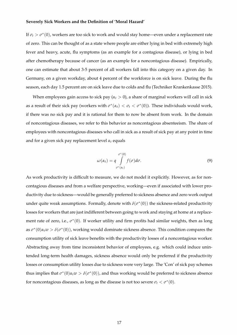
Severely Sick Workers and the Definition of ’Moral Hazard’

If σt > σ∗(0), workers are too sick to work and would stay home—even under a replacement rate

of zero. This can be thought of as a state where people are either lying in bed with extremely high

fever and heavy, acute, flu symptoms (as an example for a contagious disease), or lying in bed

after chemotherapy because of cancer (as an example for a noncontagious disease). Empirically,

one can estimate that about 3-5 percent of all workers fall into this category on a given day. In

Germany, on a given workday, about 4 percent of the workforce is on sick leave. During the flu

season, each day 1.5 percent are on sick leave due to colds and flu (Techniker Krankenkasse 2015).

When employees gain access to sick pay (αt > 0), a share of marginal workers will call in sick

as a result of their sick pay (workers with σ∗(αt) < σt < σ∗(0)). These individuals would work,

if there was no sick pay and it is rational for them to now be absent from work. In the domain

of noncontagious diseases, we refer to this behavior as noncontagious absenteeism. The share of

employees with noncontagious diseases who call in sick as a result of sick pay at any point in time

and for a given sick pay replacement level αt equals

ω(αt) = qσ∗(0)∫

σ∗(αt)

f (σ)dσ. (9)

As work productivity is difficult to measure, we do not model it explicitly. However, as for non-

contagious diseases and from a welfare perspective, working—even if associated with lower pro-

ductivity due to sickness—would be generally preferred to sickness absence and zero work output

under quite weak assumptions. Formally, denote with δ(σ∗(0)) the sickness-related productivity

losses for workers that are just indifferent between going to work and staying at home at a replace-

ment rate of zero, i.e., σ∗(0). If worker utility and firm profits had similar weights, then as long

as σ∗(0)αtw > δ(σ∗(0)), working would dominate sickness absence. This condition compares the

consumption utility of sick leave benefits with the productivity losses of a noncontagious worker.

Abstracting away from time inconsistent behavior of employees, e.g. which could induce unin-

tended long-term health damages, sickness absence would only be preferred if the productivity

losses or consumption utility losses due to sickness were very large. The ’Con’ of sick pay schemes

thus implies that σ∗(0)αtw > δ(σ∗(0)), and thus working would be preferred to sickness absence

for noncontagious diseases, as long as the disease is not too severe σt < σ∗(0).

17

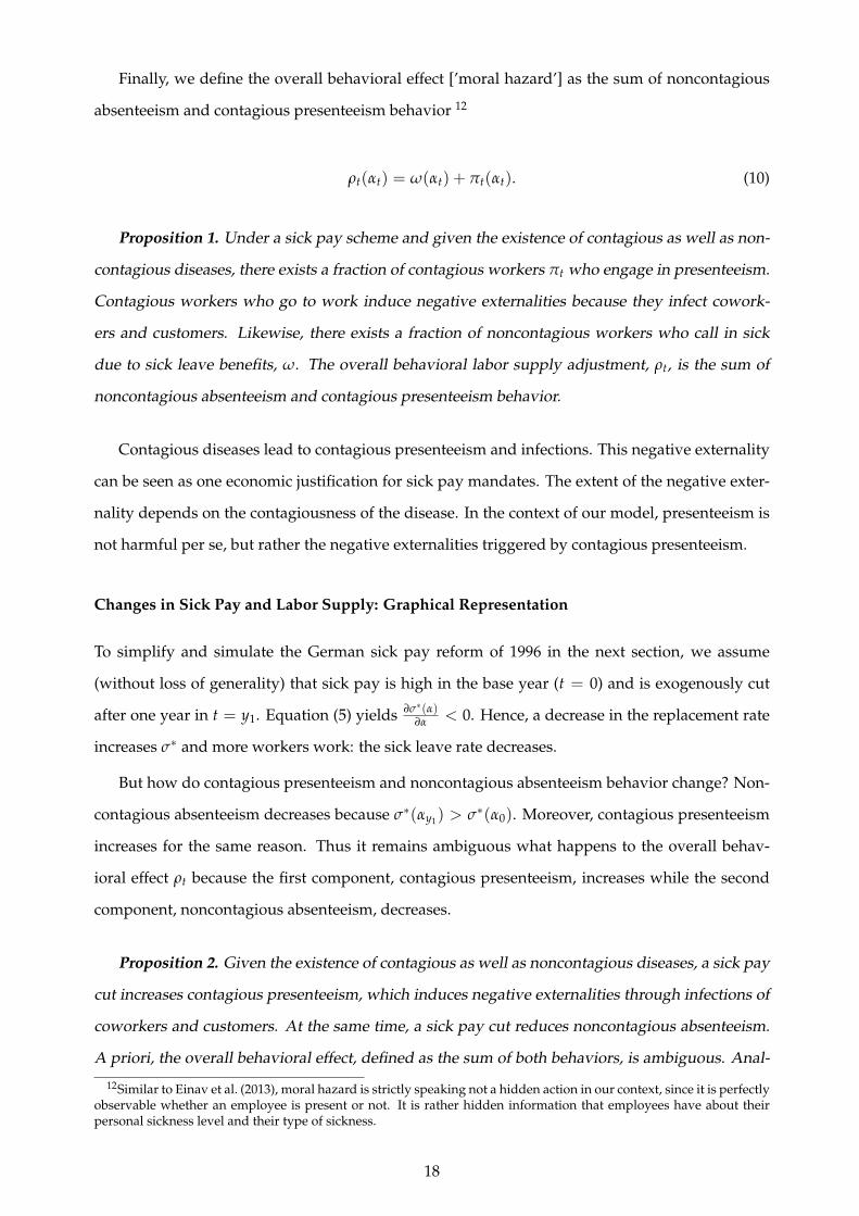
Finally, we define the overall behavioral effect [’moral hazard’] as the sum of noncontagious

absenteeism and contagious presenteeism behavior 12

ρt(αt) = ω(αt) + πt(αt). (10)

Proposition 1. Under a sick pay scheme and given the existence of contagious as well as non-

contagious diseases, there exists a fraction of contagious workers πt who engage in presenteeism.

Contagious workers who go to work induce negative externalities because they infect cowork-

ers and customers. Likewise, there exists a fraction of noncontagious workers who call in sick

due to sick leave benefits, ω. The overall behavioral labor supply adjustment, ρt, is the sum of

noncontagious absenteeism and contagious presenteeism behavior.

Contagious diseases lead to contagious presenteeism and infections. This negative externality

can be seen as one economic justification for sick pay mandates. The extent of the negative exter-

nality depends on the contagiousness of the disease. In the context of our model, presenteeism is

not harmful per se, but rather the negative externalities triggered by contagious presenteeism.

Changes in Sick Pay and Labor Supply: Graphical Representation

To simplify and simulate the German sick pay reform of 1996 in the next section, we assume

(without loss of generality) that sick pay is high in the base year (t = 0) and is exogenously cut

after one year in t = y1. Equation (5) yields ∂σ∗(α)∂α < 0. Hence, a decrease in the replacement rate

increases σ∗ and more workers work: the sick leave rate decreases.

But how do contagious presenteeism and noncontagious absenteeism behavior change? Non-

contagious absenteeism decreases because σ∗(αy1) > σ∗(α0). Moreover, contagious presenteeism

increases for the same reason. Thus it remains ambiguous what happens to the overall behav-

ioral effect ρt because the first component, contagious presenteeism, increases while the second

component, noncontagious absenteeism, decreases.

Proposition 2. Given the existence of contagious as well as noncontagious diseases, a sick pay

cut increases contagious presenteeism, which induces negative externalities through infections of

coworkers and customers. At the same time, a sick pay cut reduces noncontagious absenteeism.

A priori, the overall behavioral effect, defined as the sum of both behaviors, is ambiguous. Anal-

12Similar to Einav et al. (2013), moral hazard is strictly speaking not a hidden action in our context, since it is perfectlyobservable whether an employee is present or not. It is rather hidden information that employees have about theirpersonal sickness level and their type of sickness.

18

ogously, an increase in sick pay decreases contagious presenteeism and increases noncontagious

absenteeism behavior.

[Insert Figure 2 about here]

Figure 2 shows a graphical representation of Proposition 2. Panel A depicts the situation for non-

contagious diseases. Initially, the share of employees who engage in noncontagious absenteeism—

indicated by the sum of the two dark gray areas—is quite large. As sick pay decreases, more

workers with noncontagious illnesses come to work and the absenteeism rate decreases.

Panel B depicts the situation for contagious diseases. As sick pay decreases, contagious pre-

senteeism increases, meaning more workers with contagious illnesses come to work. Because of

additional infections, the share of individuals with a contagious disease, pt, increases, as repre-

sented by the outward shift of the density function.

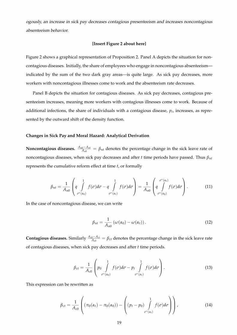
Changes in Sick Pay and Moral Hazard: Analytical Derivation

Noncontagious diseases. An0−AntAn0

= βnt denotes the percentage change in the sick leave rate of

noncontagious diseases, when sick pay decreases and after t time periods have passed. Thus βnt

represents the cumulative reform effect at time t, or formally

βnt =1

An0

q1∫

σ∗(α0)

f (σ)dσ− q1∫

σ∗(αt)

f (σ)dσ

=1

An0

qσ∗(αt)∫

σ∗(α0)

f (σ)dσ

. (11)

In the case of noncontagious disease, we can write

βnt =1

An0(ω(α0)−ω(αt)) . (12)

Contagious diseases. Similarly Ac0−ActAc0

= βct denotes the percentage change in the sick leave rate

of contagious diseases, when sick pay decreases and after t time periods.

βct =1

Ac0

p0

1∫σ∗(α0)

f (σ)dσ− pt

1∫σ∗(αt)

f (σ)dσ

. (13)

This expression can be rewritten as

βct =1

Ac0

(π0(αt)− π0(α0))−

(pt − p0)

1∫σ∗(αt)

f (σ)dσ

, (14)

19

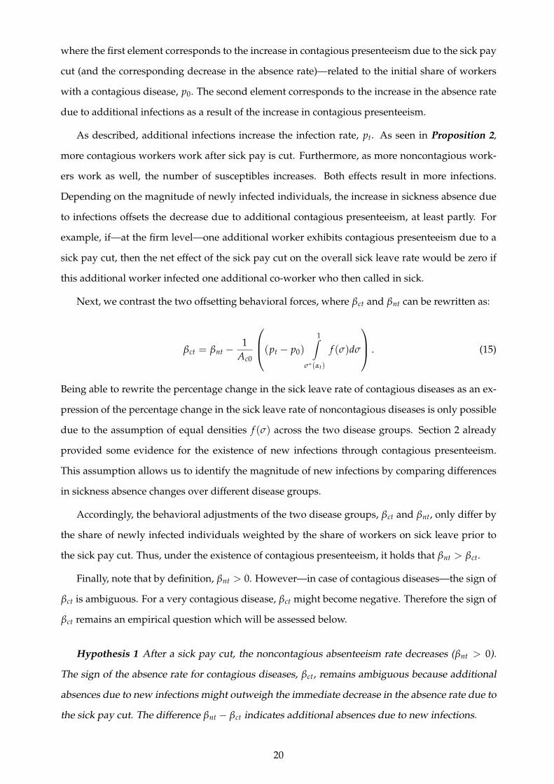
where the first element corresponds to the increase in contagious presenteeism due to the sick pay

cut (and the corresponding decrease in the absence rate)—related to the initial share of workers

with a contagious disease, p0. The second element corresponds to the increase in the absence rate

due to additional infections as a result of the increase in contagious presenteeism.

As described, additional infections increase the infection rate, pt. As seen in Proposition 2,

more contagious workers work after sick pay is cut. Furthermore, as more noncontagious work-

ers work as well, the number of susceptibles increases. Both effects result in more infections.

Depending on the magnitude of newly infected individuals, the increase in sickness absence due

to infections offsets the decrease due to additional contagious presenteeism, at least partly. For

example, if—at the firm level—one additional worker exhibits contagious presenteeism due to a

sick pay cut, then the net effect of the sick pay cut on the overall sick leave rate would be zero if

this additional worker infected one additional co-worker who then called in sick.

Next, we contrast the two offsetting behavioral forces, where βct and βnt can be rewritten as:

βct = βnt −1

Ac0

(pt − p0)

1∫σ∗(αt)

f (σ)dσ

. (15)

Being able to rewrite the percentage change in the sick leave rate of contagious diseases as an ex-

pression of the percentage change in the sick leave rate of noncontagious diseases is only possible

due to the assumption of equal densities f (σ) across the two disease groups. Section 2 already

provided some evidence for the existence of new infections through contagious presenteeism.

This assumption allows us to identify the magnitude of new infections by comparing differences

in sickness absence changes over different disease groups.

Accordingly, the behavioral adjustments of the two disease groups, βct and βnt, only differ by

the share of newly infected individuals weighted by the share of workers on sick leave prior to

the sick pay cut. Thus, under the existence of contagious presenteeism, it holds that βnt > βct.

Finally, note that by definition, βnt > 0. However—in case of contagious diseases—the sign of

βct is ambiguous. For a very contagious disease, βct might become negative. Therefore the sign of

βct remains an empirical question which will be assessed below.

Hypothesis 1 After a sick pay cut, the noncontagious absenteeism rate decreases (βnt > 0).

The sign of the absence rate for contagious diseases, βct, remains ambiguous because additional

absences due to new infections might outweigh the immediate decrease in the absence rate due to

the sick pay cut. The difference βnt − βct indicates additional absences due to new infections.

20

Finally, we denote the overall percentage change in the absence rate with βt =∆AA0

:

βt =1

A0

(ω(α0)−ω(αt)) + (π0(αt)− π0(α0))−

(pt − p0)

1∫σ∗(αt)

f (σ)dσ

. (16)

The next subsection discusses how these effects can be empirically identified in order to quantify

the change in shirking and in new infections following a change in sick pay coverage.

Identifying Contagious Presenteeism and Negative Externalities Empirically

Using Population-Level Influenza Rates to Identify Contagious Presenteeism

Section 2 exploited the implementation of U.S. sick pay mandates across space and over time in

order to test for decreased contagious presenteeism and infections after the introduction of sick

pay. We use Google Flu Trends data at the weekly regional level from 2003 to 2015 to estimate the

effect of sick pay mandates. Providing employees with paid sick leave is equivalent to increasing

sick leave benefit levels which, according to our model and a rich literature (Johansson and Palme

1996, 2005; De Paola et al. 2014; Ziebarth and Karlsson 2010, 2014; Dale-Olsen 2014; Fevang et al.

2014), unambiguously increases sick leave utilization ( ∂σ∗(α)∂α < 0).

Our model would predict that access to sick pay coverage reduces contagious presenteeism

(Proposition 2 ). This leads to a reduction in the share of individuals infected by a contagious

disease. Assume there is no sick pay at time zero (t = 0), and that sick pay is introduced after one

year (t = y1). Then the reduction in contagious diseases at t, φt, can be defined as

φt = (pt − p0) f (σ). (17)

In Section 2 we empirically tested whether φt < 0; i.e., whether sick pay coverage reduces the

incidence rate of infectious diseases in the population. We found φt < 0 which yields empirical

evidence for a reduction in contagious workplace presenteeism because employees have been

covered by paid sick leave schemes.

Furthermore, access to paid sick leave increases noncontagious absenteeism and decreases

contagious presenteeism behavior (Hypothesis 1 ). The finding of a subsequent decrease in infec-

tion rates are thus a direct implication of our model and yields strong evidence for a decrease in

contagious workplace presenteeism.

21

Using Disease-Specific Sick Leave Rates to Identify Contagious Presenteeism

To directly implement the model, one needs data on sick leave behavior, an exogenous sick pay

reform and different groups of affected workers. Then one can empirically estimate the causal

effect of the change in sick pay on the share of workers who call in sick. In the notation above, we

thus empirically identify βt.

Moreover, if one can empirically identify two different disease categories, c and n, and the

share of workers who call in sick with certified sickness due to contagious and noncontagious

diseases, one could carry out a statistical test to check if βnt > βct. In other words, one could test

if a sick-pay-cut induced decrease in sick leave is larger for disease categories, n as compared to

c, which would yield evidence for an increased spread of contagious diseases via an increase in

contagious presenteeism behavior.

Proposition 4a. Given the existence of a reform that exogenously varied sick pay and sick

leave data on differently affected employees, one can econometrically test if βt > 0, i.e., if the

labor supply adjustment with respect to a sick pay cut is positive and, if so, how large it is.

Proposition 4b. Given the availability of data for contagious and noncontagious sick leave

rates, one can estimate βnt and βct. The size of βnt is informative for the relevance of nonconta-

gious absenteeism behavior. βct represents both the increase in contagious presenteeism and in

additional sick leave due to infections triggered by contagious presenteeism behavior.

Proposition 4c. Lastly, one can econometrically test if βnt > βct (Hypothesis 1), i.e., whether

the labor supply adjustment is larger for noncontagious than for contagious diseases. The size

of the differential illustrates additional infections that lead to additional sick leave as a result of

contagious presenteeism. These represent negative externalities under lower sick pay.

The next section exploits German sick pay reforms and data on disease-specific sick leave rates to

illustrate how one can implement the second proposed test that, under the model assumptions,

empirically identifies noncontagious absenteeism and contagious presenteeism behavior.

4 Evidence from German Sick Leave Reforms

4.1 The German Employer Sick Pay Mandate

Germany has one of the most generous universal sick leave systems in the world. The system is

predominantly based on employer mandates. In Germany, employers are mandated to continue

22

wage payments for up to six weeks per sickness episode. In other words, employers have to

provide 100 percent sick pay from the first day of a period of sickness without benefit caps.13

In the case of illness, employees are obliged to inform their employer immediately about both

the sickness and the expected duration. From the fourth day of a sickness episode, a doctor’s

certificate is required. However, employers have the right to ask for a doctor’s note from day

one of a spell, and many employees voluntarily submit doctors’ notes from day one. Note that

the sickness itself remains confidential. Employees just have to inform their employer that they

are sick, not why, and the standardized form for the doctor’s note does not indicate the type of

disease, which is confidentially transmitted to the sickness fund. This is important because the

model assumes that the type of disease is unobservable to the employer.

If the sickness lasts more than six continuous weeks, the doctor needs to issue a different

certificate. From the seventh week onward, sick pay is disbursed by the health insurers (called

“sickness funds”) and lowered to 70 percent of foregone gross wages for those who are insured

under Statutory Health Insurance (SHI).14

4.2 The Policy Reforms of 1996 and 1999

Sick Pay Cut at the End of 1996

In 1996, the center-right government passed a Bill to Foster Growth and Employment, effective

October 1, 1996. Panel A of Table C1 in the appendix summarizes how the bill altered the federal

employer mandate. The most important provision of the bill reduced the minimum statutory sick

pay level from 100 percent to 80 percent of foregone wages.15 In addition to Table C1, Ziebarth

and Karlsson (2010, 2014) provide more details on the regulatory changes and affected employee

groups. This paper solely focuses on the implementation at the industry level among private

sector employees who were covered by collective agreements.

Ongoing union pressure made employer associations in various industries—through collec-

tive agreements—to voluntarily provide sick pay on top of the statutory regulations. Further, the

question of whether employees in specific industries were entitled to claim 100 percent or 80 per-

13In principle, there is no limit to the frequency of sick leave spells. However, if employees fall sick again due tothe same illness after an episode of six weeks, the law explicitly states that they are only again eligible for employer-provided sick pay if at least six months have been passed between the two spells or twelve month have been passedsince the beginning of the first spell. This paragraph intends to avoid substitution of long-term spells by short-termspells.

14 Two additional benefit caps limit long-term sick pay. The first cap is 90 percent of the net wage, and the secondcap is the contribution ceiling up to which contribution rates have to be paid.

15 In addition to this bill, another bill cut SHI long-term sick pay from the seventh week onward from 80 percent to70 percent of forgone gross wages. Ziebarth (2013) shows that this second bill did not induce significant behavioralreactions among the long-term sick.

23

cent of their salary during sickness episodes was determined by existing collective agreements

and their legal interpretation. Some existing agreements explicitly, but probably coincidentally,

stated that sick pay would be 100 percent, while others did not mention sick pay at all. In the

former case, sick pay would remain 100 percent despite the decrease in the generosity of the em-

ployer mandate, whereas in the latter case, sick pay would decrease to 80 percent until a revised

agreement was negotiated.

Review of collective agreements. We reviewed all collective agreements that existed during

the time of the sick pay reforms and categorized industries (Hans Bockler Stiftung 2014). Over-

all, one can distinguish three different groups and industries: Panel B of Table C1 provides the

provisions at the industry level and our categorization.

Group I is composed of the construction sector, whose collective agreement covered about 1.1

million private sector workers. When the law was passed in 1996, the existing collective agree-

ment did not include any explicit provision on sick pay, which is why the entire federal regulations

applied to the construction sector at the time of the bill’s implementation. A negotiated compro-

mise between unions and employers resulted in a new agreement which became effective July 1,

1997. This new agreement specified that the cut in the replacement rate would only be applied

during the first three days of a sickness episode.16

Group II counts at least 4.4 million covered employees and is quantitatively the largest group.

It includes 11 industries as specified in the notes to Table C1, among them the steel, textile and

automobile industry. Union leaders in these industries managed to maintain the symbolically

important 100 percent sick pay level. However, in return, they agreed to exclude paid overtime

from the basis of calculation for sick pay, which effectively means that employees with a significant

amount of overtime hours experienced sick pay cuts.17

16In 1997 a minimum wage in the construction sector was introduced. Theoretically a wage increase should also leadto a reduction in sickness absence. Blien et al. (2009) and Rattenhuber (2011) find a positive impact of the law on wagesin East Germany. Whereas we cannot ultimately rule out an impact on sick leave rates, we consider it very unlikely thatover proportional wage increases for low-wage blue collar construction workers in East Germany are the major driverof the large effects identified below. In any case, they are no threat to the illustration of the application of our testingprocedure.

17 There are several reasons why this type of sick pay cut may be of minor relevance: (a) Fraction of EmployeesEffectively Affected. As representative SOEPGroup (2008) data show, among BKK insurees (which our main data set iscomposed of), only 19% had paid overtime hours in 1998, the average being 4 hours per week. (b) Size of Cut. Whereasa decrease in the base rate to 80% would reduce net sick pay by e 280 per month (in 1998 values), the exclusion ofpaid overtime would only lead to a net cut of e 110 per month, conditional on working overtime and getting paidfor it. (c) Salience of Cut. While maintaining the 100% replacement level had a high symbolic meaning for unions, theindirect reductions in sick pay were not communicated as openly, and it is questionable if every employee was aware ofthem. (d) Affected individuals. One could suspect that employees with paid overtime hours might be highly motivatedemployees in leading positions with a low number of sick days and a low propensity to shirk. However, as the SOEPshows, employees with paid overtime had on average 10 sick days per year while those without paid overtime hourshad only 4.7 sick days.

24

Group III is composed of seven industries, all of which stated in their collective agreements

that they would maintain 100 percent sick pay. Moreover, in contrast to Group II, these industries

did not exclude overtime payments from the basis of calculation. Hence the 4 million employees

covered by these agreements serve as control group in the evaluation of the 1997 sick pay cut.

Reversal of Main Sick Pay Cut 1999 and Remaining Changes

After the federal election was won by the new center-left coalition in 1998, as a reaction to the

1996 bill, the Bill for Social Insurance Corrections and to Protect Employee Rights was passed

and became effective January 1, 1999. It increased federally mandated sick pay again from 80

percent to 100 percent. However, as Table C1 illustrates, while the main provision was reversed,

two minor—but potentially important—details made the new arrangements less generous than

sick pay coverage prior to October 1996. And in combination with the meanwhile negotiated

collective agreements, they affected the three groups in Table C1 differently.

First, the four week waiting period—introduced in October 1996—was maintained. This im-

plies that new employees have not been eligible for paid sick leave during the first month of their

employment. However, to our knowledge no collective agreement had excluded the application

of this waiting period, meaning that none of the three groups was affected by this provision in

1999. Second, the 1999 bill explicitly stated that paid overtime would be excluded from the basis

of calculation. This provision was not part of the 1996 reform bill; it was probably a reaction to the

many collective agreements that had implemented such a provision at the industry level in 1997

and 1998. However, because no industry in Group I and III of Table C1 excluded paid overtime

voluntary in their 1997/1998 agreements, ironically, Group III’s sick pay became less generous as

a result of the 1999 center-left bill.

4.3 Exploiting Administrative Data on Disease-Specific Sickness Absence: 1994–2004

In Germany, information on certified sickness absence—including diagnoses—are collected by the

nonprofit SHI sickness funds covering 90 percent of the population (Gesetzliche Krankenversicherun-

gen GKV). In 1995, before the first reform, switching between health plans was not possible and

employees were assigned to company-based health plans (Betriebskrankenkassen, BKKs) if their em-

ployer offered such plans (similar to the employer-sponsored health plans in the U.S. but with

mandatory enrollment). In 1995, a total of 960 SHI sickness funds existed, and 690 or 72 percent

of them were company-based health plans (German Federal Statistical Office 2014). Employees

25

covered by these health plans were likely also covered by binding collective agreements. (Eibich

et al. 2012; Schmitz and Ziebarth forthcoming).

The Federal Association of Company-Based Sickness Funds (BKK Dachverband) annually pub-

lishes sick leave statistics of their 4.8 million enrollees (19 percent of all private sector employees)

who are mandatorily SHI insured and gainfully employed (Bundesverband der Betriebskrankenkassen

(BKK) 2004).18 The Krankheitsartenstatistik reports both the incidence as well as the length of

sickness spells by gender, age group, diagnoses according to the International Classification of

Diseases (ICD), and industry. We collected and digitized information from annual reports be-

tween 1994 and 2004.19 Note that the data are only published by the main disease category as

defined by the ICD; we have no discretion on how to categorize the different disease groups. The

descriptive statistics are in the appendix, Table C2.

In total, we count 1,188 observations, where each observation represents one industry and year

as well as the diagnosed sickness category. More specifically, we count 11 years and 18 industries,

which adds up to 198 industry-year observations per diagnosis category.

Generated sick leave variables. Our outcome variable is the sick leave rate. This variable

counts the number of certified sickness episodes per 100 enrollees (sick cases per 100 enrollees).

We transform each dependent variable by taking the logarithm. The log-transformation is mainly

done because βnt in equation (11) as well as βct in equation (13) are expressed in percent and we

would like to link the model to the empirical part as closely as possible.

Figure 3a shows the distribution of total sick cases per 100 enrollees and Figure 3b its log-

arithm. In both cases we observe relatively symmetric, close to normal, distributions. The un-

transformed plain variable has a mean of 125, implying 1.25 sick leave cases per year and enrollee

across all industries and years. However, the variation ranges from 90 to 163 (Figure 3a and Table

C2).

[Insert Figure 3 about here]

Looking at the disease categories and their incidence rates, one finds that the largest disease

group is respiratory diseases, ICD codes J00-J99, contributing 29 percent of all cases. Within this

18Although, strictly speaking, BKKs are not legally obliged to contribute to the Krankheitsartenstatistik, the over-whelming majority does, probably simply out of tradition to contribute to this important statistic that has been existingsince 1976. In 2013, more than 90 percent of all mandatorily insured BKK enrollees were covered by the Krankheit-sartenstatistik (BKK 2004; German Federal Statistical Office 2014). There is no evidence that this share systematicallyvaried due to the reforms.

19We cannot use earlier data due to a lack of consistency that goes back to an earlier reform. Although the datacontain information on the duration of sickness spells by disease groups, we decided to not exploit this information asthe theoretical predictions of the reforms on the duration of spells are ambiguous.

26

group, a third of all cases are due to “bronchitis (J20)”, while a quarter is due to “influenza (J09).”

Moreover, another fifth are caused by “acute upper respiratory infections (J06).”

The second largest disease group with almost 20 percent of all cases is musculoskeletal diseases

(M00-M99), which have the reputation to be particularly prone to shirking behavior. The most

noteworthy subcategory in this group is “dorsalgia - back pain (M54)” making up 70 percent of

all musculoskeletal cases.

Next in terms of their incidence relevance are digestive diseases (K00-K93, 14 percent), in-

juries and poisoning (S00-T98, 11 percent), followed by infectious diseases (A00-B99, 6 percent).

The most common digestive disease is “noninfective gastroenteritis (K52, 45 percent)”. Infectious

diseases are mainly made up of “viral infections (B34)” and “infectious gastroenteritis (A09).”

Together over 80 percent of all cases coded as infectious diseases fall in these two subcategories.

4.4 Nonparametric Graphical Evidence

Figure 3 shows the “Development of Normalized Sick Leave Cases by Treatment Groups” over

time. Figure 4a shows the development for the overall Sick leave rate, Figure 4b looks at muscu-

loskeletal diseases, and Figures 4c and d plot diseases of the respiratory system as well as infec-

tious diseases. In addition to being normalized by the number of enrollees, these graphs are also

adjusted with respect to the reference year 1994, which is indexed as 100. The two black vertical

bars indicate the official implementation dates of the decrease and increase in sick pay generos-

ity, respectively. The representation in Figure 4 serves two main purposes: 1) to examine the

plausibility of the common time assumption, and 2) to anticipate and visually illustrate the main

findings and help understand how they identify the model in the second section. Musculoskeletal

sick leave cases (e.g., back pain, Figure 4b) represent the category “non-infectious diseases” in our

model in the second section, whereas infectious sick leave cases (Figure 4d) represent the category

“infectious diseases” in our model. Respiratory sick leave cases (Figure 4c) is a mixed category.

[Insert Figure 4 about here]

Overall, Figure 4 shows us the following: First, in general the data support the common time

trend assumption. Despite some minor spikes here and there, it is obvious that all three groups

in the four graphs develop in a pretty parallel manner over the 11 years without reform. In the

graphs, this is the case for the time periods before 1997 and after 2000. In particular Figure 4d—

showing infectious diseases—illustrates a remarkably parallel development (and does not provide

any graphical evidence for a reform effect).

27

Second, with the exception of infectious diseases, the other three graphs provide strong ev-

idence of a significant reform effect for Group I (see Table C1). Immediately after the reform

implementation, we observe a 20 percent decrease in the sick leave rate for the overall disease

category.20 As for musculoskeletal diseases—the noncontagious disease category—the decrease is

almost twice as large and around -40% for Group I, suggesting strong increases in shirking behav-

ior. As for respiratory diseases—the mixed disease category that also includes flues and common

colds—the decrease is only around -10%. Finally, as for infectious disease—the contagious disease

category—we do not observe much evidence for any reform effect.

Third, the gap between the differently affected groups unambiguously, not but entirely, closes

after 2000. This suggests that the behavioral reaction after the reversal of the sick pay cut kicks in

delayed, probably due to the relatively low media coverage when the law was reversed. More-

over, there is evidence for time persistence or habit formation in sick leave behavior, since the

regulations were again identical for all three groups post-1999 (Table C1). However, we still ob-

serve significant differences in between the three groups, even as late as 2004.

Fourth, the reaction to the soft sick pay cut—excluding overtime from the basis of calculation—

was obviously asymmetric. Figure 4 does not provide much evidence that excluding overtime

affected Group II’s behavior in 1997 and 1998. However, the graphical evidence suggests that the

very same measure had a significant impact on Group III post 1999.21

Relating these findings to our model above, one can summarize that (i) there is clear evidence

for a significant and persistent decrease in the absence rate following a sick pay cut, βt > 0 (Propo-

sition 4a). Similarly, sick leave rates increase when the system becomes more generous. (ii) the

labor supply adjustment of contagious diseases is smaller (and in fact close to zero) than the ad-

justment of noncontagious diseases and thus Proposition 4c, βnt > βct, holds up. In addition, we

find a large decrease in shirking βnt > 0 whereas the increase in presenteeism outweighs addi-

tional infections βct > 0 (Proposition 4b). Finally, because (iii) βnt − βct > 0, the German sick pay

cut also led to an increase in infections (Proposition 4b).

20 This is in line with the two other existing studies evaluating this reform using SOEP data (Ziebarth and Karlsson2010; Puhani and Sonderhof 2010)

21There are two potential explanations for this finding. 1) Relevance of Relative Changes. The decrease in sick pay atthe end of 1996 was heatedly debated in German society and led to strikes. The main (media) focus was clearly on thedecrease in the overall sick pay level. It is plausible that Group II did not react since the main reference point matteredhere, which was the decrease in the default federal level. About 50 percent of all employees experienced a decrease inthe level to 80 percent (Ridinger 1997; Jahn 1998). Hence the exclusion of overtime pay was, relatively seen, negligiblefor affected workers. It may not even have been noticed by the affected employees. After unions managed to negotiatethe general sick pay level to remain at 100 percent, they marketed and emphasized this success accordingly—but eitherdid not mention, or heavily down played the overtime cut. In 1999, by contrast, the exclusion of paid overtime wasthe only regulatory change that made employees worse off. 2) LATE. Since the model identifies the Local AverageTreatment Effect (LATE), it could simply be that paid overtime was more relevant for Group III than for Group II.

28

4.5 Parametric Difference-in-Differences Model

We now estimate the following conventional parametric DiD model separately for different dis-

ease categories:

log(yit) = γi + β0+β1GroupIi ×′ 97−′ 98 + β2GroupIi ×′ 99−′ 04+ (18)

β3GroupI Ii ×′ 97−′ 98 + β4GroupI Ii ×′ 99−′ 04+

+ δt + µit

where log(yit) stands for one of our dependent sick leave measures for industry i at time t. γi

are 17 industry fixed effects and δt 10 year fixed effects. The standard errors are routinely clustered

at the industry level. We interact the treatment indicators as defined below with two time period

dummy variables ’97-’98 and ’99-’04. The reference period is the years 1994 to 1996.

GroupIi as well as GroupI Ii are binary treatment indicators. As for the 1996 reform, Group

I experienced a sick pay cut from 100 percent to 80 percent, while Group II underwent a soft

sick pay cut—with paid overtime excluded (Table C1). Group III was not affected, serving as the

control group. Thus β1 identifies the effect of the sick pay cut for Group I relative to Group III and

the years 1997/1998 and relative to the time between 1994 and 1996. Moreover, β3 identifies the

effect of excluding paid overtime for Group II in 1997/1998 relative to the pre-reform period.

As for the 1999 reform, the main pay level was increased again for Group I, but overtime

excluded from the basis of calculation. Group II was not affected and serves as control group.

Group III experienced a soft cut (Table C1). Thus, β2 identifies the post-1999 level effect, relative

to pre-1997 levels, or the joint effect of the two reforms for Group I. Moreover, the difference

β2 − β1 identifies the effect of the increase in sick pay levels from 80 percent to 100 percent after

1999 relative to 1997/1998. In contrast, β3-β4 identifies the effect of the overtime exclusion for

Group III in the post-1999 era relative to pre-1999. Recall that overtime was excluded for Group II

in 1997 while nothing happened to Group III, whereas in 1999, overtime was excluded for Group

III while nothing happened to Group II. Consequently, −β4 + β3 identifies the estimate of the

1999 overtime exclusion for Group III. Hence, we differentiate three different groups over three

different time periods but only need to estimate four relevant parameters. Since the outcome

measures are in logarithms, β1 to β4 directly provide the reform-related change of the outcome

variable in percent.

29

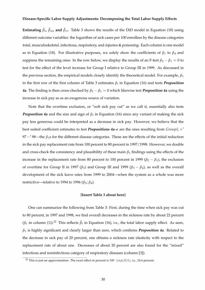
Disease-Specific Labor Supply Adjustments: Decomposing the Total Labor Supply Effects

Estimating βt, βnt, and βct. Table 3 shows the results of the DiD model in Equation (18) using

different outcome variables: the logarithm of sick cases per 100 enrollees by the disease categories

total, musculoskeletal, infectious, respiratory, and injuries & poisoning. Each column is one model

as in Equation (18). For illustrative purposes, we solely show the coefficients of β1 to β4 and

suppress the remaining ones. In the row below, we display the results of an F-test β2 − β1 = 0 to

test for the effect of the level increase for Group I relative to Group III in 1999. As discussed in

the previous section, the empirical models closely identify the theoretical model. For example, β1

in the first row of the first column of Table 3 estimates βt in Equation (16) and tests Proposition

4a. The finding is then cross-checked by β2 − β1 = 0 which likewise test Proposition 4a using the

increase in sick pay as as an exogenous source of variation.

Note that the overtime exclusion, or “soft sick pay cut” as we call it, essentially also tests

Proposition 4a and the size and sign of βt in Equation (16) since any variant of making the sick

pay less generous could be interpreted as a decrease in sick pay. However, we believe that the

best suited coefficient estimates to test Propositions 4a–c are the ones resulting from GroupIi ×′

97−′ 98—the β1s for the different disease categories. These are the effects of the initial reduction

in the sick pay replacement rate from 100 percent to 80 percent in 1997/1998. However, we double

and cross-check the consistency and plausibility of these main β1 findings using the effects of the

increase in the replacement rate from 80 percent to 100 percent in 1999 (β2 − β1), the exclusion

of overtime for Group II in 1997 (β3) and Group III and 1999 (β3 − β4), as well as the overall

development of the sick leave rates from 1999 to 2004—when the system as a whole was more

restrictive—relative to 1994 to 1996 (β2; β4).

[Insert Table 3 about here]

One can summarize the following from Table 3: First, during the time when sick pay was cut

to 80 percent, in 1997 and 1998, we find overall decreases in the sickness rate by about 22 percent

(β1 in column (1)).22 This reflects βt in Equation (16), i.e., the total labor supply effect. As seen,

β1 is highly significant and clearly larger than zero, which confirms Proposition 4a. Related to

the decrease in sick pay of 20 percent, one obtains a sickness rate elasticity with respect to the

replacement rate of about one. Decreases of about 20 percent are also found for the “mixed”

infectious and noninfectious category of respiratory diseases (column [3]).

22 This is just an approximation. The exact effect in percent is 100 · (exp(X)1), i.e., 24.6 percent.

30

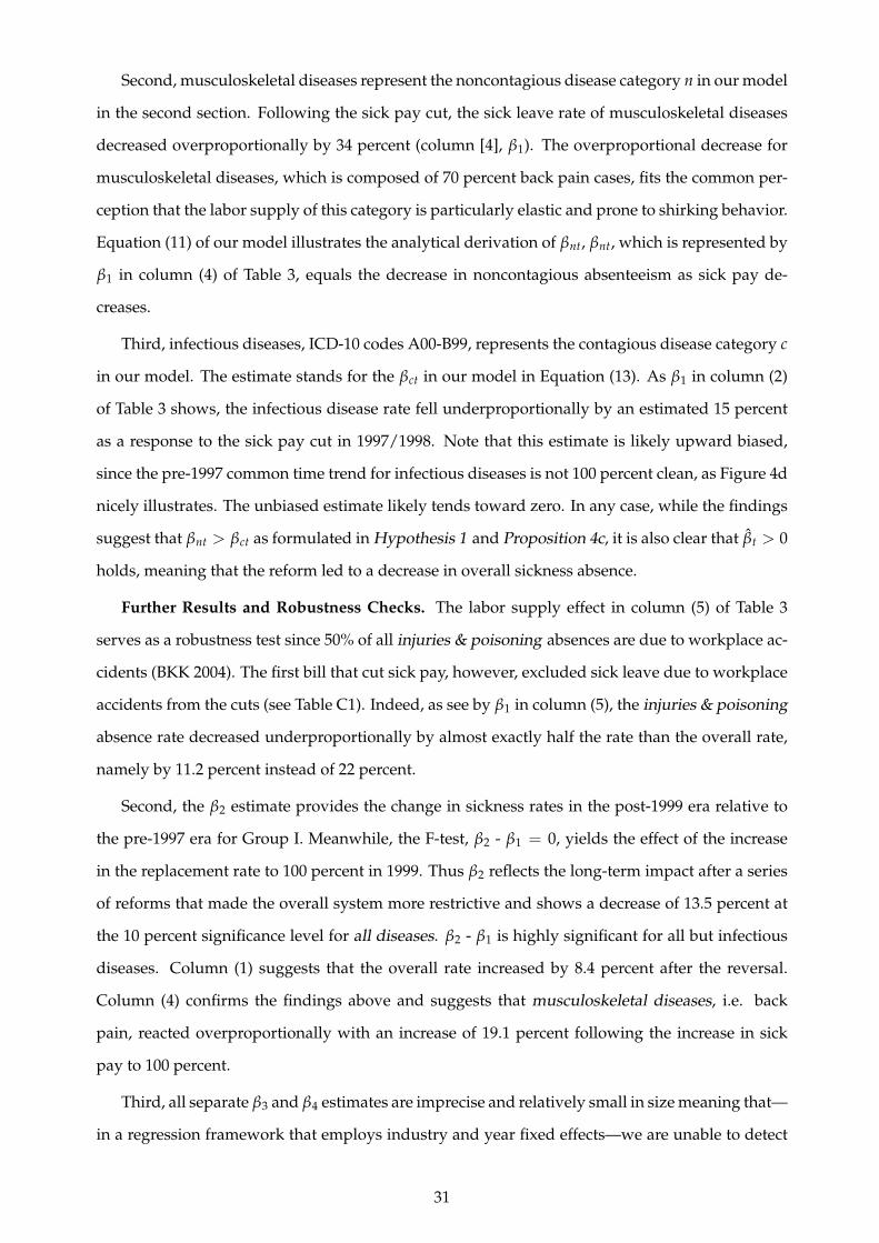
Second, musculoskeletal diseases represent the noncontagious disease category n in our model

in the second section. Following the sick pay cut, the sick leave rate of musculoskeletal diseases

decreased overproportionally by 34 percent (column [4], β1). The overproportional decrease for

musculoskeletal diseases, which is composed of 70 percent back pain cases, fits the common per-

ception that the labor supply of this category is particularly elastic and prone to shirking behavior.

Equation (11) of our model illustrates the analytical derivation of βnt, βnt, which is represented by

β1 in column (4) of Table 3, equals the decrease in noncontagious absenteeism as sick pay de-

creases.

Third, infectious diseases, ICD-10 codes A00-B99, represents the contagious disease category c

in our model. The estimate stands for the βct in our model in Equation (13). As β1 in column (2)

of Table 3 shows, the infectious disease rate fell underproportionally by an estimated 15 percent

as a response to the sick pay cut in 1997/1998. Note that this estimate is likely upward biased,

since the pre-1997 common time trend for infectious diseases is not 100 percent clean, as Figure 4d

nicely illustrates. The unbiased estimate likely tends toward zero. In any case, while the findings

suggest that βnt > βct as formulated in Hypothesis 1 and Proposition 4c, it is also clear that βt > 0

holds, meaning that the reform led to a decrease in overall sickness absence.

Further Results and Robustness Checks. The labor supply effect in column (5) of Table 3

serves as a robustness test since 50% of all injuries & poisoning absences are due to workplace ac-

cidents (BKK 2004). The first bill that cut sick pay, however, excluded sick leave due to workplace

accidents from the cuts (see Table C1). Indeed, as see by β1 in column (5), the injuries & poisoning

absence rate decreased underproportionally by almost exactly half the rate than the overall rate,

namely by 11.2 percent instead of 22 percent.

Second, the β2 estimate provides the change in sickness rates in the post-1999 era relative to

the pre-1997 era for Group I. Meanwhile, the F-test, β2 - β1 = 0, yields the effect of the increase

in the replacement rate to 100 percent in 1999. Thus β2 reflects the long-term impact after a series

of reforms that made the overall system more restrictive and shows a decrease of 13.5 percent at

the 10 percent significance level for all diseases. β2 - β1 is highly significant for all but infectious

diseases. Column (1) suggests that the overall rate increased by 8.4 percent after the reversal.

Column (4) confirms the findings above and suggests that musculoskeletal diseases, i.e. back

pain, reacted overproportionally with an increase of 19.1 percent following the increase in sick

pay to 100 percent.

Third, all separate β3 and β4 estimates are imprecise and relatively small in size meaning that—

in a regression framework that employs industry and year fixed effects—we are unable to detect

31

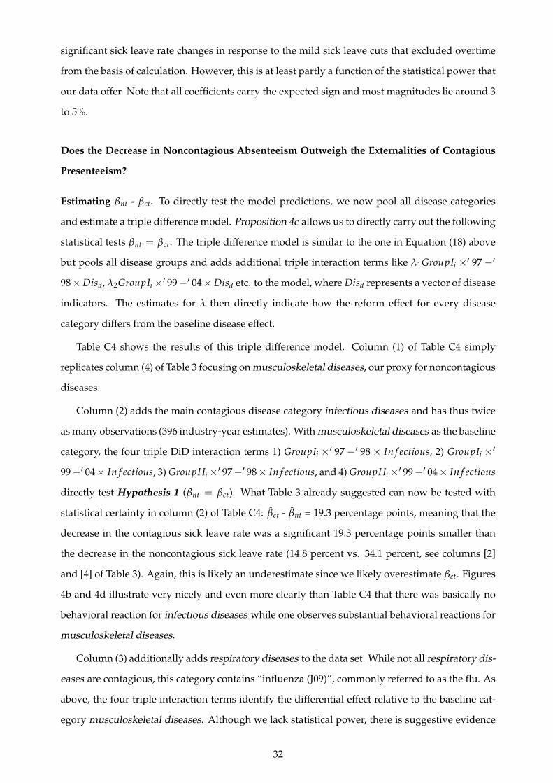
significant sick leave rate changes in response to the mild sick leave cuts that excluded overtime

from the basis of calculation. However, this is at least partly a function of the statistical power that

our data offer. Note that all coefficients carry the expected sign and most magnitudes lie around 3

to 5%.

Does the Decrease in Noncontagious Absenteeism Outweigh the Externalities of Contagious

Presenteeism?

Estimating βnt - βct. To directly test the model predictions, we now pool all disease categories

and estimate a triple difference model. Proposition 4c allows us to directly carry out the following

statistical tests βnt = βct. The triple difference model is similar to the one in Equation (18) above

but pools all disease groups and adds additional triple interaction terms like λ1GroupIi ×′ 97−′

98×Disd, λ2GroupIi×′ 99−′ 04×Disd etc. to the model, where Disd represents a vector of disease

indicators. The estimates for λ then directly indicate how the reform effect for every disease

category differs from the baseline disease effect.

Table C4 shows the results of this triple difference model. Column (1) of Table C4 simply

replicates column (4) of Table 3 focusing on musculoskeletal diseases, our proxy for noncontagious

diseases.

Column (2) adds the main contagious disease category infectious diseases and has thus twice

as many observations (396 industry-year estimates). With musculoskeletal diseases as the baseline

category, the four triple DiD interaction terms 1) GroupIi ×′ 97−′ 98× In f ectious, 2) GroupIi ×′

99−′ 04× In f ectious, 3) GroupI Ii×′ 97−′ 98× In f ectious, and 4) GroupI Ii×′ 99−′ 04× In f ectious

directly test Hypothesis 1 (βnt = βct). What Table 3 already suggested can now be tested with

statistical certainty in column (2) of Table C4: βct - βnt = 19.3 percentage points, meaning that the

decrease in the contagious sick leave rate was a significant 19.3 percentage points smaller than

the decrease in the noncontagious sick leave rate (14.8 percent vs. 34.1 percent, see columns [2]

and [4] of Table 3). Again, this is likely an underestimate since we likely overestimate βct. Figures

4b and 4d illustrate very nicely and even more clearly than Table C4 that there was basically no

behavioral reaction for infectious diseases while one observes substantial behavioral reactions for

musculoskeletal diseases.

Column (3) additionally adds respiratory diseases to the data set. While not all respiratory dis-

eases are contagious, this category contains “influenza (J09)”, commonly referred to as the flu. As

above, the four triple interaction terms identify the differential effect relative to the baseline cat-

egory musculoskeletal diseases. Although we lack statistical power, there is suggestive evidence

32

that the respiratory sick leave rate decreased by about 13 percent less than the noncontagious

baseline.

5 Conclusion

Empirically identifying presenteeism behavior is extremely challenging, yet crucial in order to test

for one major economic justification for publicly provided sick pay: the negative externalities as-

sociated with contagious presenteeism. Contagious presenteeism refers to the phenomenon when

employees with infectious diseases go to work sick and infect co-workers and customers. Such

behavior is a major public health issue and one driving force of the spread of contagious diseases.

If contagion is unobservable, which is usually the case at the beginning of sickness episodes, then

state regulation may reduce market inefficiencies by mandating employers to provide monetary

incentives for employees to stay home when sick. If such monetary incentives work, and economic

theory as well empirical studies strongly suggest that they do, then public sick pay schemes re-

duce contagious presenteeism and the spread of diseases.

To our knowledge, this study is the first that theoretically derives and empirically implements

two tests for the existence of contagious presenteeism and negative externalities in sickness insur-

ance schemes.

First, using standard DD reduced-form methods, we analyze the staggered implementation

of employer sick pay mandates at the city and state level in the U.S.—the industrialized country

with the least generous sick pay coverage. Using Google Flu Trends data, we show that influenza-

like disease rates decrease significantly when employees gain access to paid sick leave. Almost

half of all U.S. employees do not have access to sick leave insurance. Through the US sick pay

mandates, about 20K employees per 100K population gain sick leave coverage for themselves

and their children. Our estimates suggest that the relatively comprehensive laws at the level of

seven major U.S. cities helped preventing about 100 influenza-like infections per week and 100K

population. Infections rates may further decrease in the medium to long-run when employees

have accrued larger amounts of paid sick days.

The next part of the paper provides a theoretical framework illustrating the behavioral em-

ployee reactions to changes in sick pay coverage. The model defines different possible cases of

workplace absence behavior under contagious and noncontagious continuous sickness levels. As

such, we can also decompose classical ’moral hazard’ into noncontagious absenteeism and conta-

gious presenteeism behavior. The former does not imply negative health spillovers, whereas case

33

the latter does. Marginal employees with contagious diseases call in sick instead of working sick

when provided with sick leave coverage. We also derive testable conditions for the overall labor

supply effect under sickness absence insurance and its decomposed elements.

Finally, we use two German sick pay reforms and administrative physician-certified sick leave

data at the industry-level to illustrate how one can implement our proposed empirical test for the

existence of contagious presenteeism. Under the identifying conditions, we indeed find indirect

evidence for the existence of contagious presenteeism. However, assuming that the identifying

assumptions hold up, we also show that—in Germany with one of the most generous sick leave

systems worldwide—the reduction in noncontagious absenteeism was larger than the increase in

the infectious disease rate (due to contagious presenteeism) when sick pay was cut from a baseline

level of 100 percent.

Researchers could exploit different settings and our proposed methods, or variants of it, to

test for the existence and the degree of contagious presenteeism, noncontagious absenteeism, and

the overall labor supply adjustments. Important fields of applications include contagious presen-

teeism by teachers or school kids, e.g., induced by teacher or parental sick pay schemes that may

or may not cover sickness of children. Schools are important sources for the spread of contagious

diseases. Another relevant setting would be the firm level to test for contagious presenteeism

behavior by employees with a high degree of customer contact. As a last example, contagious

presenteeism behavior by health care workers can be life-threatening for patients but potentially

minimized by optimized sick pay schemes. Note that our test can be carried out using many dif-

ferent types of data, including school-level, firm-level data, or hospital-level data. Ideally, one

would want to exogenously vary the generosity of the sick pay scheme under investigation, then

measure changes in noncontagious absenteeism and contagious presenteeism behavior, and then

readjust until both undesirable employee behaviors are minimized.

More research is also needed in order to better understand how exactly contagious presen-

teeism leads to infections of coworkers and customers and how it affects overall workplace pro-

ductivity. Firm-level and employee-level compensation strategies to dampen sickness-related pro-

ductivity losses are also fruitful and relevant research questions.

ReferencesAdda, J. (2016). Economic activity and the spread of viral diseases: Evidence from high frequency

data. Quarterly Journal of Economics forthcoming, –.

Ahn, T. and J. G. Trogdon (2015). Geospatial patterns in influenza vaccination: Evidence fromuninsured and publicly insured children in North Carolina. American Journal of Infection Con-trol 43(3), 234–240.

34

Ahn, T. and A. Yelowitz (2015). The short-run impacts of Connecticuts paid sick leave legislation.Applied Economics Letters 22(15), 1267–1272.

Ahn, T. and A. Yelowitz (2016). Paid sick leave and absenteeism: The first evidence from the U.S.mimeo. https://sites.google.com/site/tomsyahn/, last accessed on May 12, 2016.

Arnott, R. and J. Stiglitz (1991). The welfare economics of moral hazard. In H. Louberg (Ed.), Risk,Information and Insurance, pp. 91–121. Springer Netherlands.

Aronsson, G., K. Gustafsson, and M. Dallner (2000). Sick but yet at work. An empirical study ofsickness presenteeism. Journal of Epidemiology & Community Health 54(7), 502–509.

Askildsen, J. E., E. Bratberg, and Ø. A. Nilsen (2005). Unemployment, labor force compositionand sickness absence: A panel study. Health Economics 14(11), 1087–1101.

Barmby, T. and M. Larguem (2009). Coughs and sneezes spread diseases: An empirical study ofabsenteeism and infectious illness. Journal of Health Economics 28(5), 1012–1017.

Barmby, T., J. Sessions, and J. G. Treble (1994). Absenteeism, efficiency wages and shirking. Scan-dinavian Journal of Economics 96(4), 561–566.

Bhattacharya, J. and M. Packalen (2012). The other ex ante moral hazard in health. Journal of HealthEconomics 31(1), 135–146.

BKK (1994-2004). Krankheitsartenstatistik. BKK Bundesverband.

Blank, P. R., M. M. Schwenkglenks, and T. D. Szucs (2009). Vaccination coverage rates in elevenEuropean countries during two consecutive influenza seasons. Journal of Infection 58(6), 446–458.

Blien, U., E. J. Jahn, G. Stephan, M. Knig, and J. Mller (2009). Impacts of minimum wages: amicrodata analysis for the German construction sector. International Journal of Manpower 30(7),716–741.

BLS (2015). Monthly state and metropolitan unemployment rates. http://download.bls.gov/pub/time.series/la/, last retrieved on September 1, 2015.

BLS (2016). Labor force statistics from the Current Population Survey: Employment-populationratio. http://data.bls.gov/timeseries/LNS12300000, last retrieved on May 11, 2016.

Bockerman, P. and E. Laukkanen (2010). What makes you work while you are sick? Evidencefrom a survey of workers. The European Journal of Public Health 20(1), 43–46.

Boots, S. W., K. Martinson, and A. Danziger (2009). Employers’ perspectives on San Francisco’spaid sick leave policy. Technical report, The Urban Institute. http://www.urban.org/publications/411868.html, last accessed on April 5, 2012.

Brown, S. (1994). Dynamic implications of absence behaviour. Applied Economics 26, 1163–1175.

Brown, S. and J. G. Sessions (1996). The economics of absence: Theory and evidence. Journal ofEconomic Surveys 10(1), 23–53.

Brown, S. and J. G. Sessions (2004). Absenteeism, presenteeism, and shirking. Economic Issues 9(1),15–23.

Bruine de Bruin, W., A. Parker, and J. Maurer (2011). Assessing small non-zero perceptions ofchance: The case of H1N1 (swine) flu risks. Journal of Risk and Uncertainty 42(2), 145–159.

Bundesverband der Betriebskrankenkassen (BKK) (1994-2004). Krankheitsartenstatistik. BKK Bun-desverband.

Busse, R. and A. Riesberg (2004). Health care systems in transition: Germany (1 ed.). WHO RegionalOffice for Europe on behalf of the European Observatory on Health Systems and Policies.

Carneiro, H. A. and E. Mylonakis (2009). Google Trends: A web-based tool for real-time surveil-lance of disease outbreaks. Clinical Infectious Diseases 49(10), 1557–1564.

Carneiro, P., K. V. Loken, and K. G. Salvanes (2015). A flying start? Maternity leave benefits andlong run outcomes of children. Journal of Political Economy 123(2), 365–412.

35

Centers for Disease Control and Prevention (2014). Final state-level influenza vaccination coverageestimates for the 2010-11 season – United States, National Immunization Survey and Behavioral RiskFactor Surveillance System, August 2010 through May 2011. CDC. http://www.cdc.gov/flu/fluvaxview/coverage_1011estimates.htm, last accessed on June 19, 2014.

Centers for Disease Control and Prevention (2016). Seasonal Influenza (Flu). CDC. http://www.cdc.gov/flu/about/disease/index.htm, last accessed on May 9, 2016.

Chatterji, M. and C. J. Tilley (2002). Sickness, absenteeism, presenteeism, and sick pay. OxfordEconomic Papers 54, 669–687.

Dahl, G. B., K. V. Loken, M. Mogstad, and K. V. Salvanes (2016). What is the case for paid maternityleave? Review of Economics and Statistics forthcoming.

Dale-Olsen, H. (2013). Absenteeism, efficiency wages, and marginal taxes. Scandinavian Journal ofEconomics 115(4), 1158–1185.

Dale-Olsen, H. (2014). Sickness absence, sick leave pay, and pay schemes. Labour 28(1), 40–63.

De Paola, M., V. Scoppa, and V. Pupo (2014). Absenteeism in the Italian public sector: The effectsof changes in sick leave policy. Journal of Labor Economics 32(2), 337–360.

Earn, D. J. D., P. W. Andrews, and B. M. Bolker (2014). Population-level effects of suppressingfever. Proceedings of the Royal Society B: Biological Sciences 281(1778).

Eibich, P., H. Schmitz, and N. R. Ziebarth (2012). Add-on premiums increase price transparency:More policy holders switch health plans. DIW Economic Bulletin 2(2), 15–24.

Einav, L., A. Finkelstein, S. P. Ryan, P. Schrimpf, and M. R. Cullen (2013). Selection on moralhazard in health insurance. The American Economic Review 103(1), 178–219.

Felder, S. (2008). To wait or to pay for medical treatment? Restraining ex-post moral hazard inhealth insurance. Journal of Health Economics 27(6), 1418–1422.

Fevang, E., S. Markussen, and K. Røed (2014). The sick pay trap. Journal of Labor Economics 32(2),305–336.

German Federal Statistical Office (2014). Federal Health Monitoring. www.gbe-bund.de, last ac-cessed on October 25, 2014.

Gilleskie, D. (2010). Work absences and doctor visits during an illness episode: The differential roleof preferences, production, and policies among men and women. Journal of Econometrics 156(1),148–163.

Gilleskie, D. B. (1998). A dynamic stochastic model of medical care use and work absence. Econo-metrica 66(1), 1–45.

Ginsberg, J., M. H. Mohebbi, R. S. Patel, L. Brammer, M. S. Smolinski, and L. Brilliant (2009).Detecting influenza epidemics using search engine query data. Nature 457(7232), 1012–1014.

Google (2015). Google Flu Trends. https://www.google.org/flutrends/about/data/flu/us/data.txt, last retrieved on September 1, 2015.

Gruber, J. (1994). The incidence of mandated maternity benefits. American Economic Review 84(3),622–641.

Hans Bockler Stiftung (2014). WSI Tarifarchiv. Deutscher Gewerkschaftsbund (DGB). http://www.boeckler.de/index_wsi_tarifarchiv.htm, last accessed on June 19, 2014.

Hesselius, P., P. Johansson, and P. Nilsson (2009). Sick of your colleagues’ absence? Journal of theEuropean Economic Association 7(2-3), 112.

Heymann, J., H. J. Rho, J. Schmitt, and A. Earle (2009). Contagion nation: a compari-son of paid sick day policies in 22 countries. Technical Report 2009-19, Center for Eco-nomic and Policy Research (CEPR). http://www.cepr.net/documents/publications/paid-sick-days-2009-05.pdf, last accessed on April 5, 2012.

36

Hirsch, B., D. S. J. Lechmann, and C. Schnabel (2015). Coming to work while sick: An economictheory of presenteeism with an application to German data. IZA Discussion Papers 9015.

Ichino, A. and G. Maggi (2000). Work environment and individual background: Explaining re-gional shirking differentials in a large Italian firm. The Quarterly Journal of Economics 115(3),1057–1090.

Ichino, A. and E. Moretti (2009). Biological gender differences, absenteeism, and the earnings gap.American Economic Journal: Applied Economics 1(1), 183–218.

Ichino, A. and R. T. Riphahn (2005). The effect of employment protection on worker effort. Acomparison of absenteeism during and after probation. Journal of the European Economic Associ-ation 3(1), 120–143.

Jahn, J. (1998). Lohnfortzahlung: Gerichte stehen vor Herkulesaufgabe. Handelsblatt July, 2, 4.

Johansson, P. and M. Palme (1996). Do economic incentives affect work absence? Empirical evi-dence using Swedish micro data. Journal of Public Economics 59(1), 195–218.

Johansson, P. and M. Palme (2002). Assessing the effect of public policy on worker absenteeism.Journal of Human Resources 37(2), 381–409.

Johansson, P. and M. Palme (2005). Moral hazard and sickness insurance. Journal of Public Eco-nomics 89(9-10), 1879–1890.

Johns, G. (2010). Presenteeism in the workplace: A review and research agenda. Journal of Organi-zational Behavior 31(4), 519–542.

Jorgensen, H. and E. Appelbaum (2014). Expanding federal family and medical leave coverage:Who benefits from changes in eligibility requirements? CEPR Reports and Issue Briefs.

Karlsson, M., T. Nilsson, and S. Pichler (2014). The impact of the 1918 Spanish flu epidemic oneconomic performance in Sweden. Journal of Health Economics 36(0), 1–19.

Kermack, W. and A. McKendrick (1927). A contribution to the mathematical theory of epidemics.Proceedings of the Royal Society of London. Series A 115(772), 700–721.

Lalive, R., A. Schlosser, A. Steinhauer, and J. Zweimuller (2014). Parental leave and mothers’careers: The relative importance of job protection and cash benefits. The Review of EconomicStudies 81(1), 219–265.

Lazer, D., R. Kennedy, G. King, and A. Vespignani (2014). Google Flu Trends still appears sick:An evaluation of the 2013-2014 flu season. Working Paper 155056, Harvard University Open-Scholar.

Lovell, V. (2003). No time to be sick: Why everyone suffers when workers don’t have paidsick leave. Policy report, Institute for Womens Policy Research. http://www.iwpr.org/publications/pubs/, last accessed at March 19, 2014.

Markussen, S. (2012). The individual cost of sick leave. Journal of Population Economics 25(4), 1287–1306.

Markussen, S., A. Mykletun, and K. Røed (2012). The case for presenteeism: Evidence from Nor-way’s sickness insurance program. Journal of Public Economics 96(11), 959–972.

Markussen, S., K. Røed, O. J. Røgeberg, and S. Gaure (2011). The anatomy of absenteeism. Journalof Health Economics 30(2), 277–292.

Maurer, J. (2009). Who has a clue to preventing the flu? Unravelling supply and demand effectson the take-up of influenza vaccinations. Journal of Health Economics 28(3), 704–717.

Mullahy, J. (1999). It’ll only hurt a second? Microeconomic determinants of who gets flu shots.Health Economics 8(1), 9–24.

Newhouse, J. P. (2006). Reconsidering the moral hazard-risk avoidance tradeoff. Journal of HealthEconomics 25(5), 1005–1014.

37

Nordberg, M. and K. Røed (2009). Economic incentives, business cycles, and long-term sicknessabsence. Industrial Relations 48(2), 203–230.

Nyman, J. A. (1999). The economics of moral hazard revisited. Journal of Health Economics 18(6),811–824.

Pauly, M. (1983). More on moral hazard. Journal of Health Economics 2(1), 81–85.

Pauly, M. V. (1974). Overinsurance and public provision of insurance: The roles of moral hazardand adverse selection. The Quarterly Journal of Economics 88(1), 44–62.

Pauly, M. V., S. Nicholson, D. Polsky, M. L. Berger, and C. Sharda (2008). Valuing reductionsin on-the-job illness: ’presenteeism’ from managerial and economic perspectives. Health Eco-nomics 17(4), 469–485.

Philipson, T. (2000). Economic epidemiology and infectious diseases. In A. J. Culyer and J. P.Newhouse (Eds.), Handbook of Health Economics, Volume 1 of Handbook of Health Economics, Chap-ter 33, pp. 1761–1799. Elsevier.

Pichler, S. (2015). Sickness absence, moral hazard, and the business cycle. Health economics 24(6),692–710.

Pichler, S. and N. R. Ziebarth (2016). Labor Market Effects of US Sick Pay Mandates. IZA Discus-sion Papers 9867.

Puhani, P. A. and K. Sonderhof (2010). The effects of a sick pay reform on absence and on health-related outcomes. The Journal of Health Economics 29(2), 285–302.

Rattenhuber, P. (2011). Building the minimum wage: Germany’s first sectoral minimum wageand its impact on wages in the construction industry. Discussion papers, German Institute forEconomic Research (DIW Berlin) 1111.

Ridinger, R. (1997). Einfluss arbeitsrechtlicher Regelungen auf die Beschaftigungsentwicklung imHandwerk–Ergebnisse von Befragungen von Handwerksbetrieben im 3. Quartal 1997. Techni-cal report, Zentralverband des Deutschen Handwerks. http://www.zdh.de, last accessed onJune 19, 2009.

Riphahn, R. T. (2004). Employment protection and effort among German employees. EconomicsLetters 85, 353–357.

Ross, R. (1916). An application of the theory of probabilities to the study of a priori pathometry.Part I. Proceedings of the Royal Society of London. Series A 92(638), 204–230.

Rossin-Slater, M., C. J. Ruhm, and J. Waldfogel (2013). The effects of California’s Paid FamilyLeave Program on mothers leave? Taking and subsequent labor market outcomes. Journal ofPolicy Analysis and Management 32(2), 224–245.

Ruhm, C. J. (1998). The economic consequences of parental leave mandates: Lessons from Europe.The Quarterly Journal of Economics 113(1), 285–317.

Ruhm, C. J. (2000). Parental leave and child health. Journal of Health Economics 19(6), 931–960.

Sandy, R. and R. F. Elliott (2005). Long-term illness and wages: The impact of the risk of occupa-tionally related long-term illness on earnings. Journal of Human Resources 40(3), 744–768.

Schmitz, H. and N. R. Ziebarth (2017). Does price framing affect the consumer price sensitivity ofhealth plan choice? Journal of Human Resources 52(1).

Scoppa, V. and D. Vuri (2014). Absenteeism, unemployment and employment protection legisla-tion: evidence from Italy. IZA Journal of Labor Economics 3(1), 1–25.

Simpson, R. (1998). Presenteeism, power and organizational change: Long hours as a career bar-rier and the impact on the working lives of women managers. British Journal of Management 9,37–50.

SOEPGroup (2008). German Socio-economic Panel Study (SOEP), data of the years 1984 2007. DOI:10.5684/soep.v24.

38

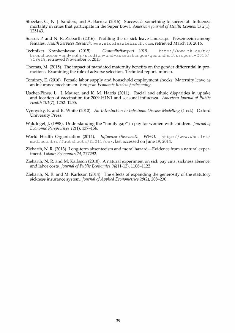
Stoecker, C., N. J. Sanders, and A. Barreca (2016). Success Is something to sneeze at: Influenzamortality in cities that participate in the Super Bowl. American Journal of Health Economics 2(1),125143.

Susser, P. and N. R. Ziebarth (2016). Profiling the us sick leave landscape: Presenteeim amongfemales. Health Services Research. www.nicolasziebarth.com, retrieved March 13, 2016.

Techniker Krankenkasse (2015). Gesundheitsreport 2015. http://www.tk.de/tk/broschueren-und-mehr/studien-und-auswertungen/gesundheitsreport-2015/718618, retrieved November 5, 2015.

Thomas, M. (2015). The impact of mandated maternity benefits on the gender differential in pro-motions: Examining the role of adverse selection. Technical report. mimeo.

Tominey, E. (2016). Female labor supply and household employment shocks: Maternity leave asan insurance mechanism. European Economic Review forthcoming.

Uscher-Pines, L., J. Maurer, and K. M. Harris (2011). Racial and ethnic disparities in uptakeand location of vaccination for 2009-H1N1 and seasonal influenza. American Journal of PublicHealth 101(7), 1252–1255.

Vynnycky, E. and R. White (2010). An Introduction to Infectious Disease Modelling (1 ed.). OxfordUniversity Press.

Waldfogel, J. (1998). Understanding the “family gap” in pay for women with children. Journal ofEconomic Perspectives 12(1), 137–156.

World Health Organization (2014). Influenza (Seasonal). WHO. http://www.who.int/mediacentre/factsheets/fs211/en/, last accessed on June 19, 2014.

Ziebarth, N. R. (2013). Long-term absenteeism and moral hazard—Evidence from a natural exper-iment. Labour Economics 24, 277292.

Ziebarth, N. R. and M. Karlsson (2010). A natural experiment on sick pay cuts, sickness absence,and labor costs. Journal of Public Economics 94(11-12), 1108–1122.

Ziebarth, N. R. and M. Karlsson (2014). The effects of expanding the generosity of the statutorysickness insurance system. Journal of Applied Econometrics 29(2), 208–230.

39

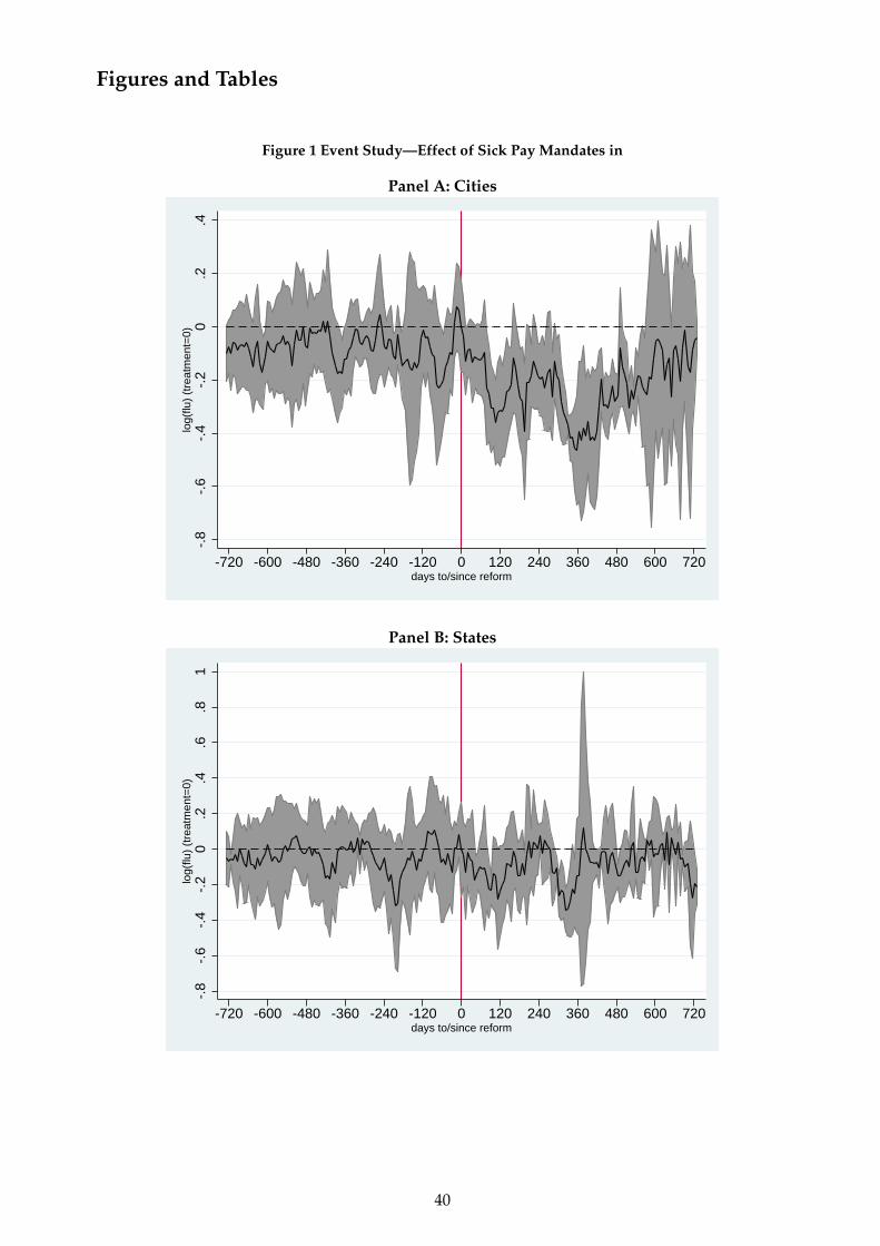
Figures and Tables

Figure 1 Event Study—Effect of Sick Pay Mandates in

Panel A: Cities-.

8-.

6-.

4-.

20

.2.4

log(

flu)

(tre

atm

ent=

0)

-720 -600 -480 -360 -240 -120 0 120 240 360 480 600 720days to/since reform

Panel B: States

-.8

-.6

-.4

-.2

0.2

.4.6

.81

log(

flu)

(tre

atm

ent=

0)

-720 -600 -480 -360 -240 -120 0 120 240 360 480 600 720days to/since reform

40

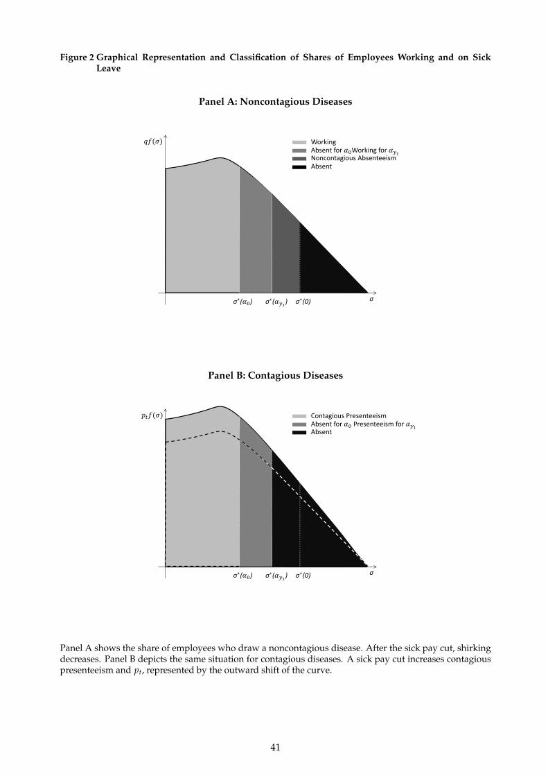
Figure 2 Graphical Representation and Classification of Shares of Employees Working and on SickLeave

Panel A: Noncontagious Diseases

σσ∗( ) σ∗( ) σ∗(0)

WorkingAbsent for Working forNoncontagious AbsenteeismAbsent

Panel B: Contagious Diseases

σσ∗( ) σ∗( ) σ∗(0)

Contagious PresenteeismAbsent for Presenteeism for Absent

Panel A shows the share of employees who draw a noncontagious disease. After the sick pay cut, shirkingdecreases. Panel B depicts the same situation for contagious diseases. A sick pay cut increases contagiouspresenteeism and pt, represented by the outward shift of the curve.

41

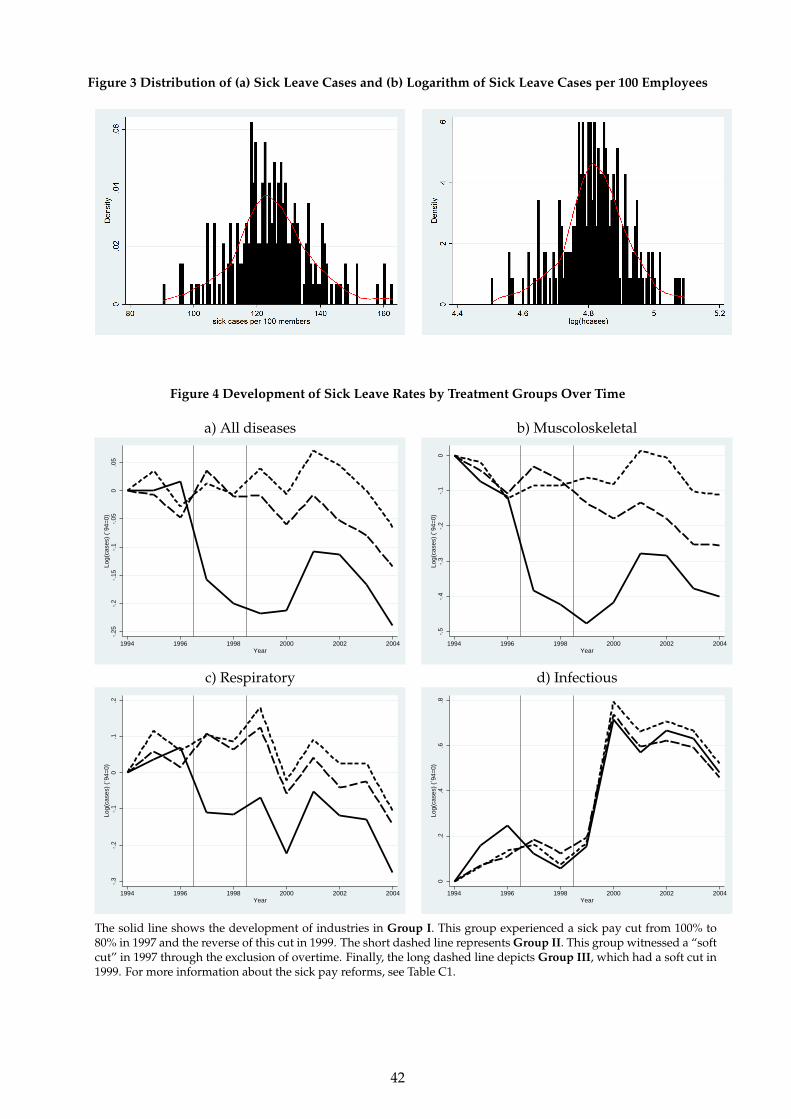
Figure 3 Distribution of (a) Sick Leave Cases and (b) Logarithm of Sick Leave Cases per 100 Employees

Figure 4 Development of Sick Leave Rates by Treatment Groups Over Time

a) All diseases b) Muscoloskeletal

-.25

-.2

-.15

-.1

-.05

0.0

5Lo

g(ca

ses)

(´9

4=0)

1994 1996 1998 2000 2002 2004Year

-.5

-.4

-.3

-.2

-.1

0Lo

g(ca

ses)

(´9

4=0)

1994 1996 1998 2000 2002 2004Year

c) Respiratory d) Infectious

-.3

-.2

-.1

0.1

.2Lo

g(ca

ses)

(´9

4=0)

1994 1996 1998 2000 2002 2004Year

0.2

.4.6

.8Lo

g(ca

ses)

(´9

4=0)

1994 1996 1998 2000 2002 2004Year

The solid line shows the development of industries in Group I. This group experienced a sick pay cut from 100% to80% in 1997 and the reverse of this cut in 1999. The short dashed line represents Group II. This group witnessed a “softcut” in 1997 through the exclusion of overtime. Finally, the long dashed line depicts Group III, which had a soft cut in1999. For more information about the sick pay reforms, see Table C1.

42

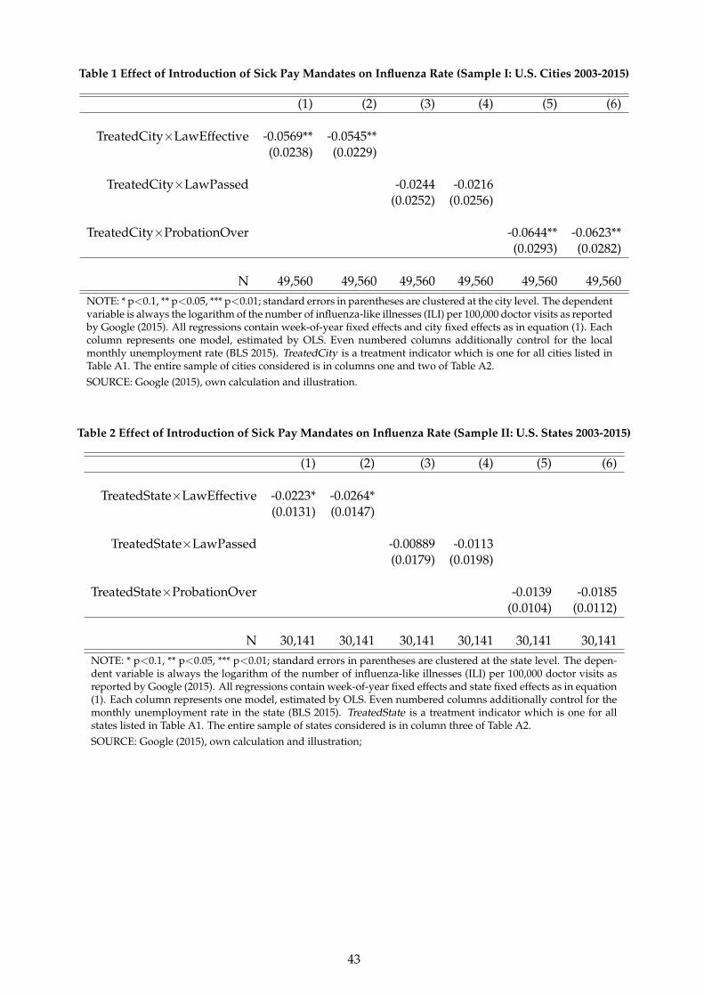
Table 1 Effect of Introduction of Sick Pay Mandates on Influenza Rate (Sample I: U.S. Cities 2003-2015)

(1) (2) (3) (4) (5) (6)

TreatedCity×LawEffective -0.0569** -0.0545**(0.0238) (0.0229)

TreatedCity×LawPassed -0.0244 -0.0216(0.0252) (0.0256)

TreatedCity×ProbationOver -0.0644** -0.0623**(0.0293) (0.0282)

N 49,560 49,560 49,560 49,560 49,560 49,560NOTE: * p<0.1, ** p<0.05, *** p<0.01; standard errors in parentheses are clustered at the city level. The dependentvariable is always the logarithm of the number of influenza-like illnesses (ILI) per 100,000 doctor visits as reportedby Google (2015). All regressions contain week-of-year fixed effects and city fixed effects as in equation (1). Eachcolumn represents one model, estimated by OLS. Even numbered columns additionally control for the localmonthly unemployment rate (BLS 2015). TreatedCity is a treatment indicator which is one for all cities listed inTable A1. The entire sample of cities considered is in columns one and two of Table A2.SOURCE: Google (2015), own calculation and illustration.

Table 2 Effect of Introduction of Sick Pay Mandates on Influenza Rate (Sample II: U.S. States 2003-2015)

(1) (2) (3) (4) (5) (6)

TreatedState×LawEffective -0.0223* -0.0264*(0.0131) (0.0147)

TreatedState×LawPassed -0.00889 -0.0113(0.0179) (0.0198)

TreatedState×ProbationOver -0.0139 -0.0185(0.0104) (0.0112)

N 30,141 30,141 30,141 30,141 30,141 30,141NOTE: * p<0.1, ** p<0.05, *** p<0.01; standard errors in parentheses are clustered at the state level. The depen-dent variable is always the logarithm of the number of influenza-like illnesses (ILI) per 100,000 doctor visits asreported by Google (2015). All regressions contain week-of-year fixed effects and state fixed effects as in equation(1). Each column represents one model, estimated by OLS. Even numbered columns additionally control for themonthly unemployment rate in the state (BLS 2015). TreatedState is a treatment indicator which is one for allstates listed in Table A1. The entire sample of states considered is in column three of Table A2.SOURCE: Google (2015), own calculation and illustration;

43

Table 3 Effect of Changes in Sick Pay on Normalized Cases of Sick Leave by Disease Groups

All diseases(1)

Infectious(2)

Respiratory(3)

Musculosk.(4)

Inj. & Pois.(5)

Group I×’97-’98 -0.220*** -0.148*** -0.208*** -0.341*** -0.112**(Effect of Cut ’97) (0.057) (0.047) (0.054) (0.076) (0.045)

Group I×’99-’04 -0.135* -0.075 -0.131*** -0.150 0.030(Level post-’99 vs. pre-’97) (0.070) (0.053) (0.044) (0.157) (0.087)

Group II×’97-’98 -0.029 -0.041 -0.022 -0.038 -0.006(Effect of Soft Cut ’97) (0.065) (0.073) (0.061) (0.086) (0.065)

Group II×’99-’04 0.053 0.053 0.017 0.131 0.107(Level post-’99 vs. pre-’97) (0.078) (0.070) (0.055) (0.164) (0.095)

[Group I×’99-’04] - [Group I×’97-’98] 0.084*** 0.073 0.077*** 0.191** 0.142***pvalue 0.000 0.121 0.000 0.032 0.004(Effect of Increase ’99)

R2 0.659 0.949 0.816 0.858 0.918Observations 198 198 198 198 198Number of industries 18 18 18 18 18NOTE: * p<0.1, ** p<0.05, *** p<0.01; standard errors in parentheses are clustered at the industry-level. All regressions areweighted by the annual number of industry-specific sickness fund enrollees. The descriptive statistics are in the Appendix (Ta-ble C2). Each column represents one model as in equation (18), estimated by OLS, i.e., all models include industry and year fixedeffects. The dependent variables are logarithms of the normalized sick leave cases per 100 employees. Column (1) employs thetotal number of sick leave cases as dependent variable, column (2) solely uses certified infectious sick leave cases and so on. Formore information on how the variables were generated, see section 2.2. Treated is a treatment indicator with one for Group I andzero for Group III, whereas PartlyTreated is one for Group II and zero for Group III. Group I experienced a sick pay cut from 100to 80% in 1997 and a reversal in 1999. Group II experienced a soft cut in 1997 and Group III experienced a soft cut in 1999. Formore information about the sick pay reforms, see Table C1.SOURCE: BKK (2004), own calculation and illustration;

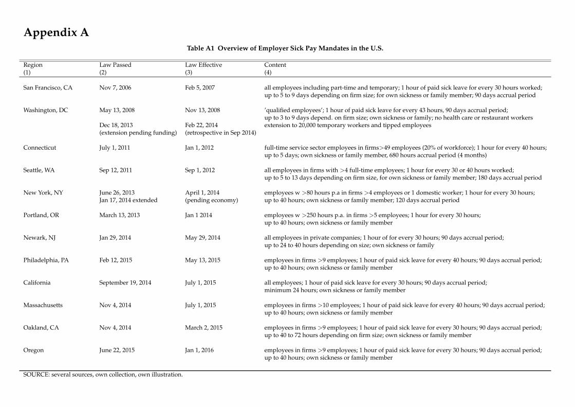
Appendix ATable A1 Overview of Employer Sick Pay Mandates in the U.S.

Region(1)

Law Passed(2)

Law Effective(3)

Content(4)

San Francisco, CA Nov 7, 2006 Feb 5, 2007 all employees including part-time and temporary; 1 hour of paid sick leave for every 30 hours worked;up to 5 to 9 days depending on firm size; for own sickness or family member; 90 days accrual period

Washington, DC May 13, 2008 Nov 13, 2008 ’qualified employees’; 1 hour of paid sick leave for every 43 hours, 90 days accrual period;up to 3 to 9 days depend. on firm size; own sickness or family; no health care or restaurant workers

Dec 18, 2013 Feb 22, 2014 extension to 20,000 temporary workers and tipped employees(extension pending funding) (retrospective in Sep 2014)

Connecticut July 1, 2011 Jan 1, 2012 full-time service sector employees in firms>49 employees (20% of workforce); 1 hour for every 40 hours;up to 5 days; own sickness or family member, 680 hours accrual period (4 months)

Seattle, WA Sep 12, 2011 Sep 1, 2012 all employees in firms with >4 full-time employees; 1 hour for every 30 or 40 hours worked;up to 5 to 13 days depending on firm size, for own sickness or family member; 180 days accrual period

New York, NY June 26, 2013 April 1, 2014 employees w >80 hours p.a in firms >4 employees or 1 domestic worker; 1 hour for every 30 hours;Jan 17, 2014 extended (pending economy) up to 40 hours; own sickness or family member; 120 days accrual period

Portland, OR March 13, 2013 Jan 1 2014 employees w >250 hours p.a. in firms >5 employees; 1 hour for every 30 hours;up to 40 hours; own sickness or family member

Newark, NJ Jan 29, 2014 May 29, 2014 all employees in private companies; 1 hour of for every 30 hours; 90 days accrual period;up to 24 to 40 hours depending on size; own sickness or family

Philadelphia, PA Feb 12, 2015 May 13, 2015 employees in firms >9 employees; 1 hour of paid sick leave for every 40 hours; 90 days accrual period;up to 40 hours; own sickness or family member

California September 19, 2014 July 1, 2015 all employees; 1 hour of paid sick leave for every 30 hours; 90 days accrual period;minimum 24 hours; own sickness or family member

Massachusetts Nov 4, 2014 July 1, 2015 employees in firms >10 employees; 1 hour of paid sick leave for every 40 hours; 90 days accrual period;up to 40 hours; own sickness or family member

Oakland, CA Nov 4, 2014 March 2, 2015 employees in firms >9 employees; 1 hour of paid sick leave for every 30 hours; 90 days accrual period;up to 40 to 72 hours depending on firm size; own sickness or family member

Oregon June 22, 2015 Jan 1, 2016 employees in firms >9 employees; 1 hour of paid sick leave for every 30 hours; 90 days accrual period;up to 40 hours; own sickness or family member

SOURCE: several sources, own collection, own illustration.

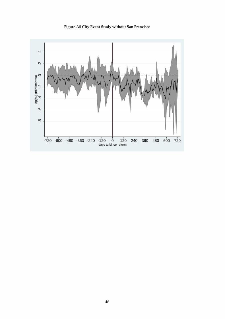
Figure A5 City Event Study without San Francisco

-.8

-.6

-.4

-.2

0.2

.4lo

g(flu

) (t

reat

men

t=0)

-720 -600 -480 -360 -240 -120 0 120 240 360 480 600 720days to/since reform

46

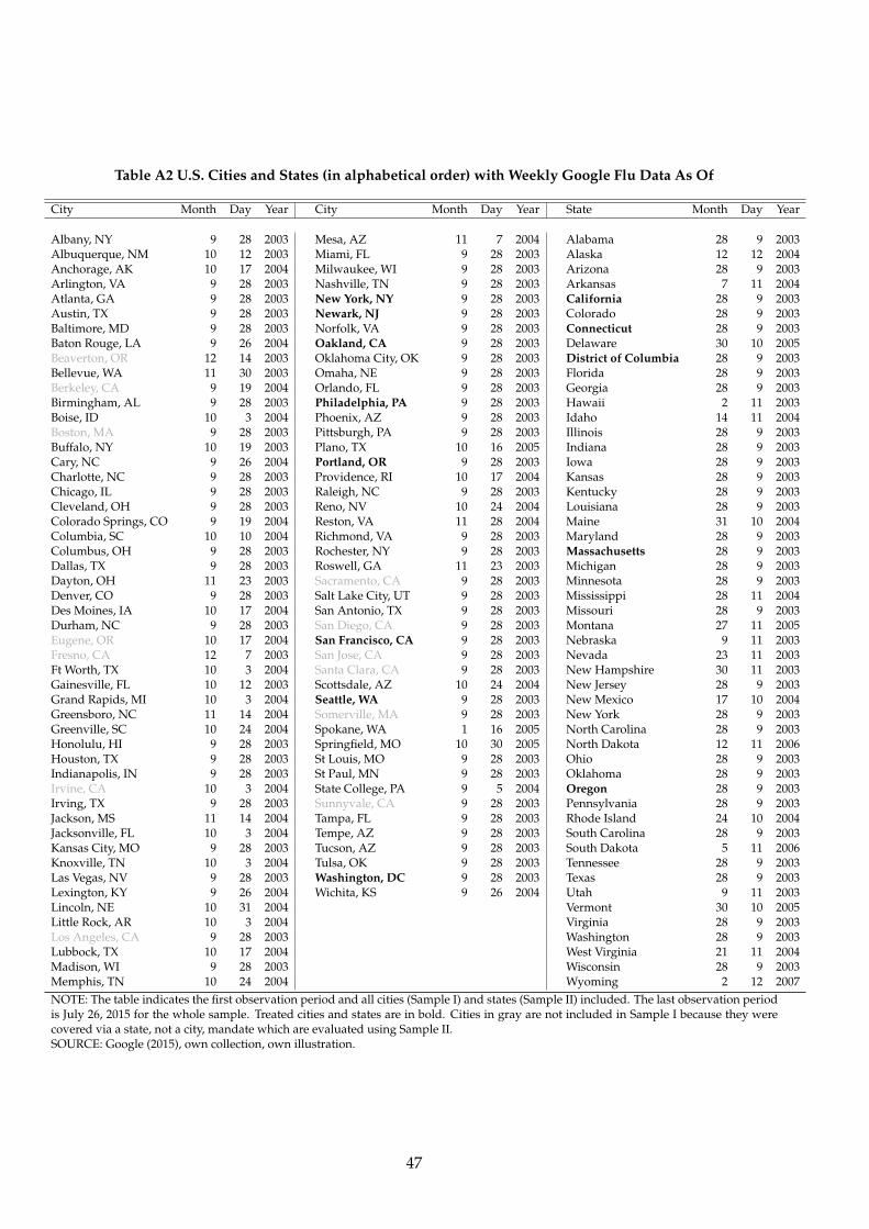
Table A2 U.S. Cities and States (in alphabetical order) with Weekly Google Flu Data As Of

City Month Day Year City Month Day Year State Month Day Year

Albany, NY 9 28 2003 Mesa, AZ 11 7 2004 Alabama 28 9 2003Albuquerque, NM 10 12 2003 Miami, FL 9 28 2003 Alaska 12 12 2004Anchorage, AK 10 17 2004 Milwaukee, WI 9 28 2003 Arizona 28 9 2003Arlington, VA 9 28 2003 Nashville, TN 9 28 2003 Arkansas 7 11 2004Atlanta, GA 9 28 2003 New York, NY 9 28 2003 California 28 9 2003Austin, TX 9 28 2003 Newark, NJ 9 28 2003 Colorado 28 9 2003Baltimore, MD 9 28 2003 Norfolk, VA 9 28 2003 Connecticut 28 9 2003Baton Rouge, LA 9 26 2004 Oakland, CA 9 28 2003 Delaware 30 10 2005Beaverton, OR 12 14 2003 Oklahoma City, OK 9 28 2003 District of Columbia 28 9 2003Bellevue, WA 11 30 2003 Omaha, NE 9 28 2003 Florida 28 9 2003Berkeley, CA 9 19 2004 Orlando, FL 9 28 2003 Georgia 28 9 2003Birmingham, AL 9 28 2003 Philadelphia, PA 9 28 2003 Hawaii 2 11 2003Boise, ID 10 3 2004 Phoenix, AZ 9 28 2003 Idaho 14 11 2004Boston, MA 9 28 2003 Pittsburgh, PA 9 28 2003 Illinois 28 9 2003Buffalo, NY 10 19 2003 Plano, TX 10 16 2005 Indiana 28 9 2003Cary, NC 9 26 2004 Portland, OR 9 28 2003 Iowa 28 9 2003Charlotte, NC 9 28 2003 Providence, RI 10 17 2004 Kansas 28 9 2003Chicago, IL 9 28 2003 Raleigh, NC 9 28 2003 Kentucky 28 9 2003Cleveland, OH 9 28 2003 Reno, NV 10 24 2004 Louisiana 28 9 2003Colorado Springs, CO 9 19 2004 Reston, VA 11 28 2004 Maine 31 10 2004Columbia, SC 10 10 2004 Richmond, VA 9 28 2003 Maryland 28 9 2003Columbus, OH 9 28 2003 Rochester, NY 9 28 2003 Massachusetts 28 9 2003Dallas, TX 9 28 2003 Roswell, GA 11 23 2003 Michigan 28 9 2003Dayton, OH 11 23 2003 Sacramento, CA 9 28 2003 Minnesota 28 9 2003Denver, CO 9 28 2003 Salt Lake City, UT 9 28 2003 Mississippi 28 11 2004Des Moines, IA 10 17 2004 San Antonio, TX 9 28 2003 Missouri 28 9 2003Durham, NC 9 28 2003 San Diego, CA 9 28 2003 Montana 27 11 2005Eugene, OR 10 17 2004 San Francisco, CA 9 28 2003 Nebraska 9 11 2003Fresno, CA 12 7 2003 San Jose, CA 9 28 2003 Nevada 23 11 2003Ft Worth, TX 10 3 2004 Santa Clara, CA 9 28 2003 New Hampshire 30 11 2003Gainesville, FL 10 12 2003 Scottsdale, AZ 10 24 2004 New Jersey 28 9 2003Grand Rapids, MI 10 3 2004 Seattle, WA 9 28 2003 New Mexico 17 10 2004Greensboro, NC 11 14 2004 Somerville, MA 9 28 2003 New York 28 9 2003Greenville, SC 10 24 2004 Spokane, WA 1 16 2005 North Carolina 28 9 2003Honolulu, HI 9 28 2003 Springfield, MO 10 30 2005 North Dakota 12 11 2006Houston, TX 9 28 2003 St Louis, MO 9 28 2003 Ohio 28 9 2003Indianapolis, IN 9 28 2003 St Paul, MN 9 28 2003 Oklahoma 28 9 2003Irvine, CA 10 3 2004 State College, PA 9 5 2004 Oregon 28 9 2003Irving, TX 9 28 2003 Sunnyvale, CA 9 28 2003 Pennsylvania 28 9 2003Jackson, MS 11 14 2004 Tampa, FL 9 28 2003 Rhode Island 24 10 2004Jacksonville, FL 10 3 2004 Tempe, AZ 9 28 2003 South Carolina 28 9 2003Kansas City, MO 9 28 2003 Tucson, AZ 9 28 2003 South Dakota 5 11 2006Knoxville, TN 10 3 2004 Tulsa, OK 9 28 2003 Tennessee 28 9 2003Las Vegas, NV 9 28 2003 Washington, DC 9 28 2003 Texas 28 9 2003Lexington, KY 9 26 2004 Wichita, KS 9 26 2004 Utah 9 11 2003Lincoln, NE 10 31 2004 Vermont 30 10 2005Little Rock, AR 10 3 2004 Virginia 28 9 2003Los Angeles, CA 9 28 2003 Washington 28 9 2003Lubbock, TX 10 17 2004 West Virginia 21 11 2004Madison, WI 9 28 2003 Wisconsin 28 9 2003Memphis, TN 10 24 2004 Wyoming 2 12 2007NOTE: The table indicates the first observation period and all cities (Sample I) and states (Sample II) included. The last observation periodis July 26, 2015 for the whole sample. Treated cities and states are in bold. Cities in gray are not included in Sample I because they werecovered via a state, not a city, mandate which are evaluated using Sample II.SOURCE: Google (2015), own collection, own illustration.

47

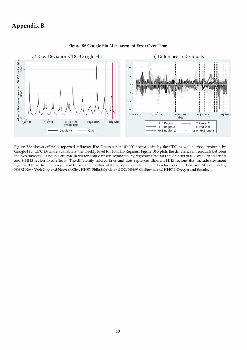
Appendix B

Figure B6 Google Flu Measurement Error Over Time

a) Raw Deviation CDC-Google Flu b) Difference in Residuals

050

0010

000

influ

enza

like

illn

ess

case

s pe

r 10

0,00

0 do

ctor

vis

its

01jul2003 01jul2006 01jul2009 01jul2012 01jul2015(mean) date

Google Flu CDC-3

-2-1

01

2

01jul2003 01jul2006 01jul2009 01jul2012 01jul2015date

HHS Region 1 HHS Region 2HHS Region 3 HHS Region 9HHS Region 10 other HHS regions

Figure B6a shows officially reported influenza-like illnesses per 100,000 doctor visits by the CDC as well as those reported byGoogle Flu. CDC Data are available at the weekly level for 10 HHS Regions. Figure B6b plots the difference in residuals betweenthe two datasets. Residuals are calculated for both datasets separately by regressing the flu rate on a set of 617 week fixed effectsand 9 HHS region fixed effects. The differently colored lines and dots represent different HHS regions that include treatmentregions. The vertical lines represent the implementation of the sick pay mandates. HHS1 includes Connecticut and Massachusetts,HHS2 New York City and Newark City, HHS3 Philadelphia and DC, HHS9 California and HHS10 Oregon and Seattle.

48

Appendix CTable C1 Detailed Overview of Reductions and Increases in German Federal Employer Sick Pay Mandates and Industry-Specific Collective Agreements

Before 10/1996(1)

10/1996–12/1998(2)

Since 1/1999(3)

Panel A: Federal Employer Mandate Regulations

100% sick pay 80% sick pay 100% sick payNo waiting period for new employees Waiting period 4 weeks Waiting period 4 weeksPaid overtime included in basis of calculation Paid overtime included in basis of calculation Paid overtime excluded in basis of calculationExtra payments included in basis of calculation Extra payments can be contractually excluded Extra payments can be contractually excluded

No cut if 1 day of paid vacation traded for 5 sick days

Panel B: Industry-Specific Collective Bargaining RegulationsGroup I 80% sick pay during first 3 days (eff. July 1, 1997)

Group II 100% sick payPaid overtime excluded in basis of calculation

Group III 100% sick pay

Panel C: Combined Effect for Different IndustriesGroup I as in Panel A 80% sick pay, since 07/’97 during first 3 days 100% sick pay

Waiting period 4 weeks Waiting period 4 weeksPaid overtime excluded in basis of calculation

Group II as in Panel A 100% sick pay 100% sick payWaiting period 4 weeks Waiting period 4 weeksPaid overtime excluded in basis of calculation Paid overtime excluded in basis of calculation

Group III as in Panel A 100% sick pay 100% sick payWaiting period 4 weeks Waiting period 4 weeks

Paid overtime excluded in basis of calculation

NOTE: Group I is composed of the construction sector. Group II contains the following industries: steel, textile, mechanical engineering, automobile, ship and aerospace, electricalengineering and optics, wood and paper, printing, food and hospitality, trade, banking and insurance. Group III represents the chemical, oil, glass, energy and water, postal andtransportation as well as public administration sector. Changes in regulation between time periods are in bold. The negotiated agreements cover 1.1M employees in Group I and atleast 4.5M in Group II and 4M in Group III (Jahn 1998; Hans Bockler Stiftung 2014).SOURCE: Hans Bockler Stiftung (2014), own illustration.

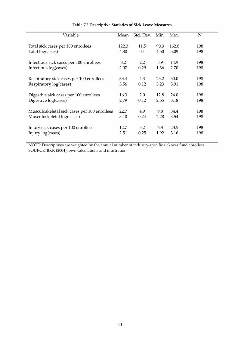
Table C2 Descriptive Statistics of Sick Leave Measures

Variable Mean Std. Dev. Min. Max. N

Total sick cases per 100 enrollees 122.3 11.5 90.3 162.8 198Total log(cases) 4.80 0.1 4.50 5.09 198

Infectious sick cases per 100 enrollees 8.2 2.2 3.9 14.9 198Infectious log(cases) 2.07 0.29 1.36 2.70 198

Respiratory sick cases per 100 enrollees 35.4 4.3 25.2 50.0 198Respiratory log(cases) 3.56 0.12 3.23 3.91 198

Digestive sick cases per 100 enrollees 16.3 2.0 12.8 24.0 198Digestive log(cases) 2.79 0.12 2.55 3.18 198

Musculoskeletal sick cases per 100 enrollees 22.7 4.9 9.8 34.4 198Musculoskeletal log(cases) 3.10 0.24 2.28 3.54 198

Injury sick cases per 100 enrollees 12.7 3.2 6.8 23.5 198Injury log(cases) 2.51 0.25 1.92 3.16 198

NOTE: Descriptives are weighted by the annual number of industry-specific sickness fund enrollees.SOURCE: BKK (2004), own calculations and illustration.

50

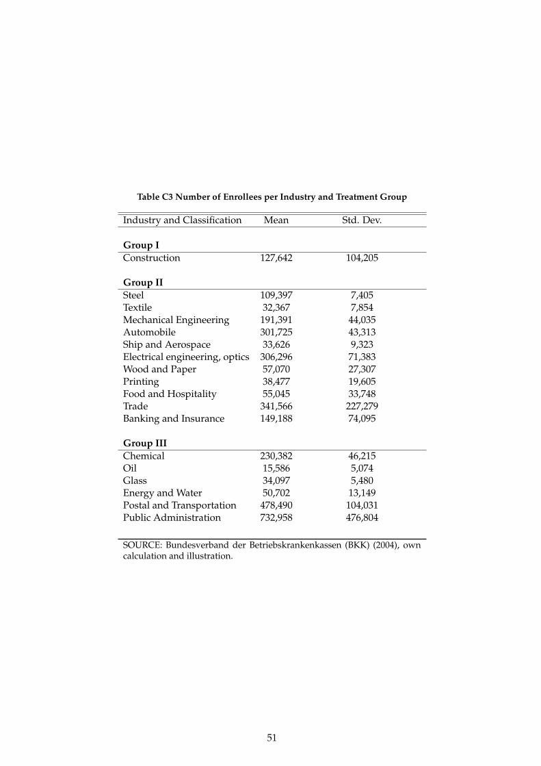
Table C3 Number of Enrollees per Industry and Treatment Group

Industry and Classification Mean Std. Dev.

Group IConstruction 127,642 104,205

Group IISteel 109,397 7,405Textile 32,367 7,854Mechanical Engineering 191,391 44,035Automobile 301,725 43,313Ship and Aerospace 33,626 9,323Electrical engineering, optics 306,296 71,383Wood and Paper 57,070 27,307Printing 38,477 19,605Food and Hospitality 55,045 33,748Trade 341,566 227,279Banking and Insurance 149,188 74,095

Group IIIChemical 230,382 46,215Oil 15,586 5,074Glass 34,097 5,480Energy and Water 50,702 13,149Postal and Transportation 478,490 104,031Public Administration 732,958 476,804

SOURCE: Bundesverband der Betriebskrankenkassen (BKK) (2004), owncalculation and illustration.

51

Table C4 Effect of Changes in Sick Pay on Normalized Cases of Sick Leave—Pooled Regressions

(1) (2) (3)Musculoskeletal Musculoskeletal, Muscul., Infect.

Infectious Respiratory

Group I×’97-’98 -0.341*** -0.341*** -0.341***(0.076) (0.075) (0.075)

Group I×’99-’04 -0.150 -0.150 -0.150(0.157) (0.155) (0.154)

Group II×’97-’98 -0.038 -0.038 -0.038(0.086) (0.085) (0.085)

Group II×’99-’04 0.131 0.131 0.131(0.164) (0.161) (0.161)

Group I×’97-’98×Infectious 0.193** 0.193**(0.088) (0.088)

Group I×’99-’04×Infectious 0.075 0.075(0.164) (0.163)

Group II×’97-’98×Infectious -0.003 -0.003(0.112) (0.111)

Group II×’99-’04×Infectious -0.079 -0.079(0.176) (0.175)

Group I×’97-’98×Respiratory 0.133(0.092)

Group I×’99-’04×Respiratory 0.019(0.160)

Group II×’97-’98×Respiratory 0.016(0.104)

Group II×’99-’04×Respiratory -0.115(0.170)

Observations 198 396 594R2 0.858 0.982 0.989NOTE: * p<0.1, ** p<0.05, *** p<0.01; standard errors in parentheses are clustered at the industry-disease-level. All regressions are weighted by the annual number of industry-specific sickness fund enrollees. Thedescriptive statistics are in the Appendix (Table C2). The regressions are based on equation 1. The modelin the first column equals the fifth column of Table 3. The model in the second column pools the two cate-gories musculoskeletal and infectious, where musculoskeletal form the reference group. The third columnadditionally adds respiratory diseases. The fourth column adds all other diseases as a separate category.All regressions are estimated by OLS and include industry, disease and year fixed effects. The dependentvariables are logarithms of the normalized sick leave cases per 100 employees. For more information onhow the variables were generated, see Section 4.3. Treated is a treatment indicator with one for Group I andzero for Group III, whereas PartlyTreated is one for Group II and zero for Group III. Group I experienceda sick pay cut from 100 to 80% in 1997 and a reversal in 1999. Group II experienced a soft cut in 1997 andGroup III experienced a soft cut in 1999. For more information about the sick pay reforms, see Table C1.SOURCE: Bundesverband der Betriebskrankenkassen (BKK) (2004), own calculation and illustration;

52