The Private Memory of Aggregate Uncertainty

Carlos E. da Costa1 Vitor F. Luz2

1Fundacao Getulio Vargas

2Yale University

FGV - May, 2011

Introduction

The ModelEnvironmentThe Planner’s ProblemMain Results

Macro Consequences

DiscussionExtensions and CaveatsRelated Literature

Conclusion

Table of Contents

Introduction

The ModelEnvironmentThe Planner’s ProblemMain Results

Macro Consequences

DiscussionExtensions and CaveatsRelated Literature

Conclusion

Introduction

Efficient provision of social insurance, aggregate risk sharing andredistribution: fundamental issues in macroeconomics and publicfinance.

Analytical framework provided by NDPF literature.

Aggregate uncertainty almost always assumed away: precludesour addressing how policies ought to vary with business cycle.

Multi-period Mirrlees’ setting with aggregate uncertainty.Choose ’convenient’ functional forms.

Characterize (as much as possible) efficient allocations in thepresence of aggregate uncertainty

How to optimally spread distortions across time and states ofthe world.Role of Memory

Normative?

Introduction

Efficient provision of social insurance, aggregate risk sharing andredistribution: fundamental issues in macroeconomics and publicfinance.

Analytical framework provided by NDPF literature.

Aggregate uncertainty almost always assumed away: precludesour addressing how policies ought to vary with business cycle.

Multi-period Mirrlees’ setting with aggregate uncertainty.Choose ’convenient’ functional forms.

Characterize (as much as possible) efficient allocations in thepresence of aggregate uncertainty

How to optimally spread distortions across time and states ofthe world.Role of Memory

Normative?

Introduction

Efficient provision of social insurance, aggregate risk sharing andredistribution: fundamental issues in macroeconomics and publicfinance.

Analytical framework provided by NDPF literature.

Aggregate uncertainty almost always assumed away: precludesour addressing how policies ought to vary with business cycle.

Multi-period Mirrlees’ setting with aggregate uncertainty.

Choose ’convenient’ functional forms.

Characterize (as much as possible) efficient allocations in thepresence of aggregate uncertainty

How to optimally spread distortions across time and states ofthe world.Role of Memory

Normative?

Introduction

Efficient provision of social insurance, aggregate risk sharing andredistribution: fundamental issues in macroeconomics and publicfinance.

Analytical framework provided by NDPF literature.

Aggregate uncertainty almost always assumed away: precludesour addressing how policies ought to vary with business cycle.

Multi-period Mirrlees’ setting with aggregate uncertainty.Choose ’convenient’ functional forms.

Characterize (as much as possible) efficient allocations in thepresence of aggregate uncertainty

How to optimally spread distortions across time and states ofthe world.Role of Memory

Normative?

Introduction

Efficient provision of social insurance, aggregate risk sharing andredistribution: fundamental issues in macroeconomics and publicfinance.

Analytical framework provided by NDPF literature.

Aggregate uncertainty almost always assumed away: precludesour addressing how policies ought to vary with business cycle.

Multi-period Mirrlees’ setting with aggregate uncertainty.Choose ’convenient’ functional forms.

Characterize (as much as possible) efficient allocations in thepresence of aggregate uncertainty

How to optimally spread distortions across time and states ofthe world.Role of Memory

Normative?

Introduction

Efficient provision of social insurance, aggregate risk sharing andredistribution: fundamental issues in macroeconomics and publicfinance.

Analytical framework provided by NDPF literature.

Aggregate uncertainty almost always assumed away: precludesour addressing how policies ought to vary with business cycle.

Multi-period Mirrlees’ setting with aggregate uncertainty.Choose ’convenient’ functional forms.

Characterize (as much as possible) efficient allocations in thepresence of aggregate uncertainty

How to optimally spread distortions across time and states ofthe world.Role of Memory

Positive: What are the ’macro’ consequences?

The Positive Questions

Macro Consequences

Procedure:

DGP is repeated Mirrlees economyGenerate aggregate dataTry to ’rationalize’ data with Representative Agent economyIn particular: Labor Wedge and Capital Wedge (Asset pricing?)

Some Answers

Labor Wedge counter(pro)-cyclical if risk aversion greater(less)than oneState-price deflators are greater (smaller) than that of RA ifrisk aversion is greater (less) than one.

The Positive Questions

Macro Consequences

Procedure:

DGP is repeated Mirrlees economyGenerate aggregate dataTry to ’rationalize’ data with Representative Agent economyIn particular: Labor Wedge and Capital Wedge (Asset pricing?)

Some Answers

Labor Wedge counter(pro)-cyclical if risk aversion greater(less)than oneState-price deflators are greater (smaller) than that of RA ifrisk aversion is greater (less) than one.

Normative or Positive?

Many institutional arrangements implement an allocation.

Assume that whatever they are, institutions implement the(possibly constrained) optimum.

Focus is shifted from specific formal arrangements toallocations.

Townsend (1994), Attanasio and Pavoni (2008), Ales andMaziero (2009), Kocherlakota and Pistaferri (2007, 2008,2009), Sleet (2006).

Table of Contents

Introduction

The ModelEnvironmentThe Planner’s ProblemMain Results

Macro Consequences

DiscussionExtensions and CaveatsRelated Literature

Conclusion

The Model

Environment

Continuum of measure one of ex-ante identical individuals,each living for T periods.

Preferences over deterministic sequences of consumption, c,effort, l, bundles are identical and of the form,∑T

t=1βt−1 {u(ct)− h(lt)}

u, h : R+ → R smooth, with u′, h′,−u′′, h′′ > 0.

In each period agents are subject to productivity shocksθt ∈ Θ =

{θ, θ}

for t = 1, .., T , with θ > θ.

In each period, aggregate shock zt ∈ Z ≡ {z, z}, withz > z > 0, affects the economy’s technology. zt = (z1, ..., zt)denote the history of aggregate shocks up to period t.

Idiosyncratic shocks are private information while aggregateshocks are publicly observed.

In each period agents are subject to productivity shocksθt ∈ Θ =

{θ, θ}

for t = 1, .., T , with θ > θ.

In each period, aggregate shock zt ∈ Z ≡ {z, z}, withz > z > 0, affects the economy’s technology. zt = (z1, ..., zt)denote the history of aggregate shocks up to period t.

Idiosyncratic shocks are private information while aggregateshocks are publicly observed.

Aggregate shocks are i.i.d. with associated probability π(z)(πt(z

t) =∏ts=1 π(zs))

Conditional on zt, idiosyncratic shocks, θt, are drawn from theprobability measure µt independent of zt

Law of large numbers applies: at period t state zt, thecross-sectional distribution of agents coincides with theex-ante distribution µt.

θt follows a Markov process: µ(θ′|θ)Assume µ(θ|θ) ≥ µ(θc|θ) for θ, θc = θ, θ

Consider various degrees of persistence.

Aggregate shocks are i.i.d. with associated probability π(z)(πt(z

t) =∏ts=1 π(zs))

Conditional on zt, idiosyncratic shocks, θt, are drawn from theprobability measure µt independent of zt

Law of large numbers applies: at period t state zt, thecross-sectional distribution of agents coincides with theex-ante distribution µt.

θt follows a Markov process: µ(θ′|θ)Assume µ(θ|θ) ≥ µ(θc|θ) for θ, θc = θ, θ

Consider various degrees of persistence.

Technology is linear: one unit of efficient labor, y = lzθ,produces one unit of consumption, c.

An allocation is (c, y) = {(ct, yt)}Tt=1, where(ct(θ

t, zt), yt(θt, zt)) is a (θt, zt)−measurable function that

denotes the bundle allocated to an agent with history θt atperiod t, when aggregate history is zt.

We say that an allocation x is resource feasible if∑µt(θt) [ct(θ

t, zt)− yt(θt, zt)]≤ 0, for all t, zt.

A benevolent planner maximizes individuals’ expected utility,∑t

βt−1∑zt

∑θt

µt(θt)πt(z

t) {u(ct)− h(lt)} .

We find optimal allocations using a direct revelationmechanism.

A reporting strategy, σ = {σt}Tt=1, is a sequence of mappingsσt : Zt ×Θt → Θ, which associate to every history

(zt, θt

)an

announcement θ.

Let U (c, y;σ) ≡

E

[∑t

βt−1

{u(ct(σt(θ

t, zt), zt)− h(yt(σt(θ

t, zt), zt)

θtzt

)}].

An allocation (c, y) is incentive compatible if

U (c, y;σ∗) ≥ U (c, y;σ) , for all σ ∈ Σ,

where σ∗t(θt, zt

)= θt for all t, θt, zt.

The Planner’s Program

max∑t

βt−1∑θt

∑zt

πt(zt)µt

(θt) [u(c(θt, zt)

)− h

(y(θt, zt)

θtzt

)]subject to ∑

θt

µt(θt) [c(θt, zt)− y(θt, zt)

]≤ 0

and

∑t

βt−1∑θt

∑zt

πt(zt)µt

(θt) [u(c(θt, zt)

)− h

(y(θt, zt)

θtzt

)]≥

∑t

βt−1∑θt

∑zt

πt(zt)µt

(θt) [u(c(σ(.), zt

))− h

(y(σ(.), zt

)θtzt

)]

for all σ ∈ Σ.

Separability and Memory

Definition

If an allocation is such that in period t there are functionsη : Z → R+ and (c, y) : Θt × Zt−1 → R2

+ such that(ct(θ

t, zt), ct(θt, zt)) = (ct(θ

t, zt−1), ct(θt, zt−1))η(zt) we say that

it is separable at t.

Definition

If an allocation is separable at t for all t we say it is separable.

Definition

If an allocation is such that, for all t, it is independent of zt−s

∀s > 1, i.e., (c(θt, zt), y(θt, zt)) = (c(θt, zt), y(θt, zt)) for some(c, y) : Θt × Z → <2

+, then we say it is memoryless.

Separability and Memory

Definition

If an allocation is such that in period t there are functionsη : Z → R+ and (c, y) : Θt × Zt−1 → R2

+ such that(ct(θ

t, zt), ct(θt, zt)) = (ct(θ

t, zt−1), ct(θt, zt−1))η(zt) we say that

it is separable at t.

Definition

If an allocation is separable at t for all t we say it is separable.

Definition

If an allocation is such that, for all t, it is independent of zt−s

∀s > 1, i.e., (c(θt, zt), y(θt, zt)) = (c(θt, zt), y(θt, zt)) for some(c, y) : Θt × Z → <2

+, then we say it is memoryless.

Separability and Memory

Definition

If an allocation is such that in period t there are functionsη : Z → R+ and (c, y) : Θt × Zt−1 → R2

+ such that(ct(θ

t, zt), ct(θt, zt)) = (ct(θ

t, zt−1), ct(θt, zt−1))η(zt) we say that

it is separable at t.

Definition

If an allocation is separable at t for all t we say it is separable.

Definition

If an allocation is such that, for all t, it is independent of zt−s

∀s > 1, i.e., (c(θt, zt), y(θt, zt)) = (c(θt, zt), y(θt, zt)) for some(c, y) : Θt × Z → <2

+, then we say it is memoryless.

Separability and Memory

Definition

If an allocation is such that in period t there are functionsη : Z → R+ and (c, y) : Θt × Zt−1 → R2

+ such that(ct(θ

t, zt), ct(θt, zt)) = (ct(θ

t, zt−1), ct(θt, zt−1))η(zt) we say that

it is separable at t.

Definition

If an allocation is separable at t for all t we say it is separable.

Definition

If an allocation is such that, for all t, it is independent of zt−s

∀s > 1, i.e., (c(θt, zt), y(θt, zt)) = (c(θt, zt), y(θt, zt)) for some(c, y) : Θt × Z → <2

+, then we say it is memoryless.

Isoelastic Preferences

u (c) =c1−ρ

1− ρand h (l) =

lγ

γ,

for ρ > 0, ρ 6= 1 and γ > 1. For ρ = 1 take u (c) = ln c.

With these preferences,

Representative agent with these preferences and no savings:C(z) = Y (z) = κzγ/(γ+ρ−1).

Individuals’ allocations

c(θ, z) = κczγ/(γ+ρ−1) and y(θ, z) = κyθγzγ/(γ+ρ−1),

with κc = {∑µ(θ)θγ}

γ−1γ+ρ−1 κy =

∑µ(θ)θγ

Isoelastic Preferences

u (c) =c1−ρ

1− ρand h (l) =

lγ

γ,

for ρ > 0, ρ 6= 1 and γ > 1. For ρ = 1 take u (c) = ln c.

With these preferences,

Representative agent with these preferences and no savings:C(z) = Y (z) = κzγ/(γ+ρ−1).

Individuals’ allocations

c(θ, z) = κczγ/(γ+ρ−1) and y(θ, z) = κyθγzγ/(γ+ρ−1),

with κc = {∑µ(θ)θγ}

γ−1γ+ρ−1 κy =

∑µ(θ)θγ

Isoelastic Preferences

u (c) =c1−ρ

1− ρand h (l) =

lγ

γ,

for ρ > 0, ρ 6= 1 and γ > 1. For ρ = 1 take u (c) = ln c.

With these preferences,

Representative agent with these preferences and no savings:C(z) = Y (z) = κzγ/(γ+ρ−1).

Individuals’ allocations

c(θ, z) = κczγ/(γ+ρ−1) and y(θ, z) = κyθγzγ/(γ+ρ−1),

with κc = {∑µ(θ)θγ}

γ−1γ+ρ−1 κy =

∑µ(θ)θγ

Inefficiency with Separable Allocations

Define ζ(z) implicitly through∑µ(θ)

{u(c(θ, z))− h

(y(θ, z)

θz

)}= u(cFB(z) [1− ζ(z)])−

∑µ(θ)h

(yFB(θ, z)

θz

)Assume c(θ, z) = c(θ)η(z) and y(θ, z) = y(θ)η(z), then

∑µ(θ)

{c(θ)1−ρ

1− ρ− y(θ)γ

γθγ

}=

[κc (1− ζ(z))]1−ρ

1− ρ− (κy)γ

γ

⇒ ζ(z) does not depend on z.

Inefficiency with Separable Allocations

Define ζ(z) implicitly through∑µ(θ)

{u(c(θ, z))− h

(y(θ, z)

θz

)}= u(cFB(z) [1− ζ(z)])−

∑µ(θ)h

(yFB(θ, z)

θz

)Assume c(θ, z) = c(θ)η(z) and y(θ, z) = y(θ)η(z), then

∑µ(θ)

{c(θ)1−ρ

1− ρ− y(θ)γ

γθγ

}=

[κc (1− ζ(z))]1−ρ

1− ρ− (κy)γ

γ

⇒ ζ(z) does not depend on z.

Proposition

The efficient allocation for the pure heterogeneity economy is ofthe form

(ct(θ, zt), yt(θ, z

t)) = (c(θ), y(θ))η(zt)

with η(z) = zγ

γ+ρ−1 , i.e., it is separable and memoryless.

In a repeated Mirrlees’ model, Werning (2007) shows taxsmoothing for h (l) = lγ

γ

Proposition

The efficient allocation for the pure heterogeneity economy is ofthe form

(ct(θ, zt), yt(θ, z

t)) = (c(θ), y(θ))η(zt)

with η(z) = zγ

γ+ρ−1 , i.e., it is separable and memoryless.

In a repeated Mirrlees’ model, Werning (2007) shows taxsmoothing for h (l) = lγ

γ

Proposition

The optimal allocation is separable in period T , i.e., there arefunctions η(zT ), c(θT , zT−1) and y(θT , zT−1) such that

c(θT , zT ) = c(θT , zT−1)η(zT ) and y(θT , zT ) = y(θT , zT−1)η(zT ).

An obvious difference between the last period and the othersis that there cannot be backloading of incentives in the lastperiod.

This suggests a connection between backloading andseparability

Proposition

The optimal allocation is separable in period T , i.e., there arefunctions η(zT ), c(θT , zT−1) and y(θT , zT−1) such that

c(θT , zT ) = c(θT , zT−1)η(zT ) and y(θT , zT ) = y(θT , zT−1)η(zT ).

An obvious difference between the last period and the othersis that there cannot be backloading of incentives in the lastperiod.

This suggests a connection between backloading andseparability

Lemma

At the optimum,

∑θt+s�θt

µ(θt+s|θt) u′(ct(θt, zt))

u′(ct+s(θt+s, zt+s))=

∑θt+s�θt

µ(θt+s|θt) u′(ct(θt, zt))

u′(ct+s(θt+s, zt+s)),

for every, θt,θt, zt and zt+s � zt.

Consider u = ln, then, letting Y(zt)

denote total production,we have

ct(θt, zt

)Y (zt)

=

∑θ′ µ

(θ′|θt

)ct+1

((θt, θ′

),(zt, z

))∑θt+1 µ (θt+1) ct+1 (θt+1, (zt, z))

=E[ct+1|θt, zt+1

]Y (zt+1)

.

Expectation in the right hand side of the expression above isconditional on zt+1

Consider u = ln, then, letting Y(zt)

denote total production,we have

ct(θt, zt

)Y (zt)

=

∑θ′ µ

(θ′|θt

)ct+1

((θt, θ′

),(zt, z

))∑θt+1 µ (θt+1) ct+1 (θt+1, (zt, z))

=E[ct+1|θt, zt+1

]Y (zt+1)

.

Expectation in the right hand side of the expression above isconditional on zt+1

Expected share of aggregate output an agent gets to consumein any aggregate state tomorrow is equal to the share ofcurrent output that she consumes today. [Demange (2008)]

That is, the expected share only depends on private history,when u(.) = ln(.)

Proposition

If period t consumption is not separable in zt, then the allocationdisplays memory in t+ s, for all s ≥ 1.

If an allocation is not separable in t, then, there must be a pairθt, θt such that c(θt, zt)/c(θt, zt) is a function of zt. From theprevious lemma, however,

c(θt, zt)ρ

c(θt, zt)ρ=

E[c(θt, θ′, zt+1)ρ|θt, zt+1

]E[c(θt, θ′, zt+1)ρ|θt, zt+1

] .Since the left hand side depends on zt, so does the right hand side.Hence, either the numerator or the denominator varies with zt.

Proposition

If period t consumption is not separable in zt, then the allocationdisplays memory in t+ s, for all s ≥ 1.

If an allocation is not separable in t, then, there must be a pairθt, θt such that c(θt, zt)/c(θt, zt) is a function of zt. From theprevious lemma, however,

c(θt, zt)ρ

c(θt, zt)ρ=

E[c(θt, θ′, zt+1)ρ|θt, zt+1

]E[c(θt, θ′, zt+1)ρ|θt, zt+1

] .Since the left hand side depends on zt, so does the right hand side.Hence, either the numerator or the denominator varies with zt.

Proposition

Let u = ln then there exist functions ct(θt) and yt(θ

t) such thatct(θ

t, zt) = ct(θt)zt and yt(θ

t, zt) = yt(θt)zt.

Rewrite the planners’ problem with the transformation of variablesc(θt, zt) = c(θt, zt)zt and y(θt, zt) = y(θt, zt)zt. Next, note that,for all t, zt disappears from the planner’s maximization.

Proposition

Let u = ln then there exist functions ct(θt) and yt(θ

t) such thatct(θ

t, zt) = ct(θt)zt and yt(θ

t, zt) = yt(θt)zt.

Rewrite the planners’ problem with the transformation of variablesc(θt, zt) = c(θt, zt)zt and y(θt, zt) = y(θt, zt)zt. Next, note that,for all t, zt disappears from the planner’s maximization.

A Two Periods Example: Idiosyncratic Risk and ρ 6= 1

T = 2

There is only one aggregate state in period 2.

Relaxed problem: only downward incentive constraints areimposed.

The planner’s relaxed problem is

max∑

µ(θ1){v1(θ1, z1) + β

∑µ(θ2|θ1)v2(θ2, z1)

}subject to

v2(θ1, θ, z1) ≥ vc2(θ1, θ, z1), θ1 = θ, θ

v1(θ, z1) + β∑

µ(θ, θ2|θ)v2(θ, θ2, z1) ≥

vc1(θ1, z1) + β∑

µ(θ, θ2|θ)v2(θ1, θ2, z1),

where,

vt(θt, zt) = u(ct(θ

t, zt))− h(yt(θ

t, zt)

θtzt

),

vct (θt, zt) = u(ct(θ

t, zt))− h(yt(θ

t, zt)

θtzt

),

and ∑µt(θ

t){ct(θ

t, z1)− yt(θt, z1)}≤ 0 t = 1, 2.

Assume the allocation is memoryless: v2(θ2, z1) = v2(θ2).

This requires separability in period 1:v1(θ1, z1) = v1(θ1)η(z1)1−ρ, and vc1(θ1, z1) = vc1(θ1)η(z1)1−ρ.

Which means that the IC constraint is[v1(θ)− vc1(θ)

]η(z1)1−ρ > β

∑µ(θ, θ2|θ)

[v2(θ, θ2)− v2(θ, θ2)

]

Assume the allocation is memoryless: v2(θ2, z1) = v2(θ2).

This requires separability in period 1:v1(θ1, z1) = v1(θ1)η(z1)1−ρ, and vc1(θ1, z1) = vc1(θ1)η(z1)1−ρ.

Which means that the IC constraint is

[v1(θ)− vc1(θ)

]η(z1)1−ρ > β

∑µ(θ, θ2|θ)

[v2(θ, θ2)− v2(θ, θ2)

]

Assume the allocation is memoryless: v2(θ2, z1) = v2(θ2).

This requires separability in period 1:v1(θ1, z1) = v1(θ1)η(z1)1−ρ, and vc1(θ1, z1) = vc1(θ1)η(z1)1−ρ.

Which means that the IC constraint is

[v1(θ)− vc1(θ)

]η(z)1−ρ = β

∑µ(θ, θ2|θ)

[v2(θ, θ2)− v2(θ, θ2)

]

Assume the allocation is memoryless: v2(θ2, z1) = v2(θ2).

This requires separability in period 1:v1(θ1, z1) = v1(θ1)η(z1)1−ρ, and vc1(θ1, z1) = vc1(θ1)η(z1)1−ρ.

Which means that the IC constraint is

[v1(θ)− vc1(θ)

]︸ ︷︷ ︸<0

η(z)1−ρ = β∑

µ(θ, θ2|θ)[v2(θ, θ2)− v2(θ, θ2)

]

Assume the allocation is memoryless: v2(θ2, z1) = v2(θ2).

This requires separability in period 1:v1(θ1, z1) = v1(θ1)η(z1)1−ρ, and vc1(θ1, z1) = vc1(θ1)η(z1)1−ρ.

Which means that the IC constraint is

[v1(θ)− vc1(θ)

]η(z)1−ρ ? β

∑µ(θ, θ2|θ)

[v2(θ, θ2)− v2(θ, θ2)

]

Assume ρ > 1

Assume the allocation is memoryless: v2(θ2, z1) = v2(θ2).

This requires separability in period 1:v1(θ1, z1) = v1(θ1)η(z1)1−ρ, and vc1(θ1, z1) = vc1(θ1)η(z1)1−ρ.

Which means that the IC constraint is

[v1(θ)− vc1(θ)

]η(z)1−ρ ? β

∑µ(θ, θ2|θ)

[v2(θ, θ2)− v2(θ, θ2)

]Assume ρ > 1

Assume the allocation is memoryless: v2(θ2, z1) = v2(θ2).

This requires separability in period 1:v1(θ1, z1) = v1(θ1)η(z1)1−ρ, and vc1(θ1, z1) = vc1(θ1)η(z1)1−ρ.

Which means that the IC constraint is

↓[v1(θ)− vc1(θ)

]η(z)1−ρ ? β

∑µ(θ, θ2|θ)

[v2(θ, θ2)− v2(θ, θ2)

]

Assume the allocation is memoryless: v2(θ2, z1) = v2(θ2).

This requires separability in period 1:v1(θ1, z1) = v1(θ1)η(z1)1−ρ, and vc1(θ1, z1) = vc1(θ1)η(z1)1−ρ.

Which means that the IC constraint is

↓ −[v1(θ)− vc1(θ)

]η(z)1−ρ ? β

∑µ(θ, θ2|θ)

[v2(θ, θ2)− v2(θ, θ2)

]

Assume the allocation is memoryless: v2(θ2, z1) = v2(θ2).

This requires separability in period 1:v1(θ1, z1) = v1(θ1)η(z1)1−ρ, and vc1(θ1, z1) = vc1(θ1)η(z1)1−ρ.

Which means that the IC constraint is

↓ −[v1(θ)− vc1(θ)

]η(z)1−ρ < β

∑µ(θ, θ2|θ)

[v2(θ, θ2)− v2(θ, θ2)

]

Generalizing...

max

T∑t=1

βt−1∑θt

∑zt

πt(zt)µt

(θt) [

u(θt, zt)− h(θt, zt)]

subject to

T∑t=1

βt−1∑θt

∑zt

πt(zt)µt

(θt) [

u(θt, zt)− h(θt, zt)]≥

T∑t=1

βt−1∑θt

∑zt

πt(zt)µt

(θt) [

u(θt, zt|σ)− h(θt, zt|σ)]

for all σ ∈ Σ,∑θt

µt(θt) [C(u(θt, zt))−Ψ(h(θt, zt))ztθt

]≤ 0

for all t, zt.

Define the price process {Qt(zt)}t and consider the alternativeprogram where∑

Qt(zt)∑θt

µt(θt) [C(u(θt, zt))−Ψ(h(θt, zt))ztθt

]≤ 0

substitutes for the period by period resource constraint.

Any solution to this program with prices{Qt(z

t)}t

such that theresource constraint holds with equality at each period, also solvesthe planner’s program.Because the planner’s program is a concave program the converseis true.

Define the price process {Qt(zt)}t and consider the alternativeprogram where∑

Qt(zt)∑θt

µt(θt) [C(u(θt, zt))−Ψ(h(θt, zt))ztθt

]≤ 0

substitutes for the period by period resource constraint.Any solution to this program with prices

{Qt(z

t)}t

such that theresource constraint holds with equality at each period, also solvesthe planner’s program.

Because the planner’s program is a concave program the converseis true.

Define the price process {Qt(zt)}t and consider the alternativeprogram where∑

Qt(zt)∑θt

µt(θt) [C(u(θt, zt))−Ψ(h(θt, zt))ztθt

]≤ 0

substitutes for the period by period resource constraint.Any solution to this program with prices

{Qt(z

t)}t

such that theresource constraint holds with equality at each period, also solvesthe planner’s program.Because the planner’s program is a concave program the converseis true.

An allocation solves the program above if and only if it solves

min∑

Qt(zt)∑θt

µt(θt) [C(u(θt, zt))−Ψ(h(θt, zt))ztθt

]subject to IC and

T∑t=1

βt−1∑θt

∑zt

πt(zt)µt

(θt) [

u(θt, zt)− h(θt, zt)]≥ w.

for some price process {Qt(zt)}t

For a given price process {Qt(zt)} it is, then, possible to focus oncomponent programs that are recursive on wt and wct defined as

wt =∑

π(z)∑

µ(θt+s|θ){ut(θ, wt, wct ; z)− ht(θ′, wt, w

ct ; z)

+βWt(θ′, wt, w

ct ; z)},

and

wct =∑

π(z)∑

µ(θ′|θc){ut(θ′, wt, wct ; z)− ht(θ′, wt, w

ct ; z)

+βWt(θ′, wt, w

ct ; z)},

An allocation is incentive compatible if and only if it satisfies

ut(θ, wt, wct ; z)− ht(θ, wt, w

ct ; z) + βWt(θ, wt, w

ct ; z) ≥

ut(θc, wt, w

ct ; z)− ht(θ

c, wt, wct ; z)

(θc

θ

)γ+ βW c

t (θc, wt, wct ; z) .

for all t ≤ T , (θ, wt, wct , z).

At the final node, define wT+1 = wcT+1 = 0.

An allocation is incentive compatible if and only if it satisfies

ut(θ, wt, wct ; z)− ht(θ, wt, w

ct ; z) + βWt(θ, wt, w

ct ; z) ≥

ut(θc, wt, w

ct ; z)− ht(θ

c, wt, wct ; z)

(θc

θ

)γ+ βW c

t (θc, wt, wct ; z) .

for all t ≤ T , (θ, wt, wct , z).

At the final node, define wT+1 = wcT+1 = 0.

Proposition

Assume that ρ 6= 1 and that types are not constant over time, thenthe optimal allocation displays memory of past aggregate shocks.

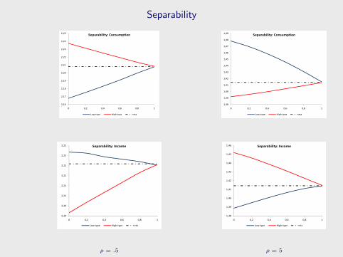
Separability

2,19

2,20

2,21

2,22

2,23

2,24

2,25Separability: Consumption

2,16

2,17

2,18

2,19

2,20

2,21

2,22

2,23

2,24

2,25

0 0,2 0,4 0,6 0,8 1

Separability: Consumption

Low type High type eta

1,42

1,43

1,44

1,45

1,46

1,47

1,48

1,49Separability: Consumption

1,38

1,39

1,40

1,41

1,42

1,43

1,44

1,45

1,46

1,47

1,48

1,49

0 0,2 0,4 0,6 0,8 1

Separability: Consumption

Low type High type eta

2,21

2,21

2,21

2,21

2,21 Separability: Income

2,20

2,20

2,21

2,21

2,21

2,21

2,21

2,21

0 0,2 0,4 0,6 0,8 1

Separability: Income

Low type High type eta

1,41

1,42

1,43

1,44

1,45

1,46 Separability: Income

1,38

1,39

1,40

1,41

1,42

1,43

1,44

1,45

1,46

0 0,2 0,4 0,6 0,8 1

Separability: Income

Low type High type eta

ρ = .5 ρ = 5

Incentives

-0,1

0

0,1

0,2

0,3

0,4

0 0,2 0,4 0,6 0,8 1

Backloading

-0,4

-0,3

-0,2

-0,1

0

0,1

0,2

0,3

0,4

0 0,2 0,4 0,6 0,8 1

Backloading

L1 H1 L2 H2

-0,02

0

0,02

0,04

0,06

0,08

0,1

0 0,2 0,4 0,6 0,8 1

Backloading

-0,1

-0,08

-0,06

-0,04

-0,02

0

0,02

0,04

0,06

0,08

0,1

0 0,2 0,4 0,6 0,8 1

Backloading

L1 H1 L2 H2

2,80%

3,80%

4,80%

5,80%

6,80%

7,80%

8,80% Individual Wedges

-0,20%

0,80%

1,80%

2,80%

3,80%

4,80%

5,80%

6,80%

7,80%

8,80%

0 0,2 0,4 0,6 0,8 1

Individual Wedges

L1 H1 L2 H2

19,80%

24,80%

29,80%

34,80%

39,80%

44,80%

49,80%Individual Wedges

-0,20%

4,80%

9,80%

14,80%

19,80%

24,80%

29,80%

34,80%

39,80%

44,80%

49,80%

0 0,2 0,4 0,6 0,8 1

Individual Wedges

L1 H1 L2 H2

ρ = .5 ρ = 5

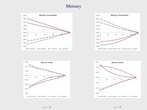
Memory

0,00%

0,50%

1,00%

1,50%

2,00%

2,50%

0 0,2 0,4 0,6 0,8 1

Memory: Consumption

-2,00%

-1,50%

-1,00%

-0,50%

0,00%

0,50%

1,00%

1,50%

2,00%

2,50%

0 0,2 0,4 0,6 0,8 1

Memory: Consumption

LL11/HL11 LL12/HL12 LL21/HL21 LL22/HL22

0,00%

1,00%

2,00%

3,00%

4,00%

5,00%

0 0,2 0,4 0,6 0,8 1

Memory: Consumption

-4,00%

-3,00%

-2,00%

-1,00%

0,00%

1,00%

2,00%

3,00%

4,00%

5,00%

0 0,2 0,4 0,6 0,8 1

Memory: Consumption

LL11/HL11 LL12/HL12 LL21/HL21 LL22/HL22

-0,10%

0,00%

0,10%

0,20%

0,30%

0 0,2 0,4 0,6 0,8 1

Memory: Income

-0,40%

-0,30%

-0,20%

-0,10%

0,00%

0,10%

0,20%

0,30%

0 0,2 0,4 0,6 0,8 1

Memory: Income

LL11/HL11 LL12/HL12 LL21/HL21 LL22/HL22

-2,00%

0,00%

2,00%

4,00%

6,00%

0 0,2 0,4 0,6 0,8 1

Memory: Income

-6,00%

-4,00%

-2,00%

0,00%

2,00%

4,00%

6,00%

0 0,2 0,4 0,6 0,8 1

Memory: Income

LL11/HL11 LL12/HL12 LL21/HL21 LL22/HL22

ρ = .5 ρ = 5

Table of Contents

Introduction

The ModelEnvironmentThe Planner’s ProblemMain Results

Macro Consequences

DiscussionExtensions and CaveatsRelated Literature

Conclusion

Macro Consequences

Labor Wedge

Output is

Y (zt) ≡∑θt−1

∑θ

µt(θt−1, θ)y(θt−1, θ, zt−1, z)

Hours are

L(zt−1, z) ≡∑θt−1

∑θ

µt(θt−1, θ)

y(θt−1, θ, zt−1, z)

θz

Aggregate Productivity is W (zt) = Y (zt)/L(zt)Consumption is

C(zt) ≡∑θt−1

∑θ

µt(θt−1, θ)c(θt−1, θ, zt−1, z)

Using C(z) = Y (z) we define the Labor Wedge

τ(z) = W (z)−γY (z)ρ+γ−1.

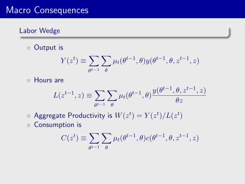
Macro Consequences

Labor Wedge

Output is

Y (zt) ≡∑θt−1

∑θ

µt(θt−1, θ)y(θt−1, θ, zt−1, z)

Hours are

L(zt−1, z) ≡∑θt−1

∑θ

µt(θt−1, θ)

y(θt−1, θ, zt−1, z)

θz

Aggregate Productivity is W (zt) = Y (zt)/L(zt)Consumption is

C(zt) ≡∑θt−1

∑θ

µt(θt−1, θ)c(θt−1, θ, zt−1, z)

Using C(z) = Y (z) we define the Labor Wedge

τ(z) = W (z)−γY (z)ρ+γ−1.

The Separable Case: c(θ, zt) = c(θ)η(zt), and y(θ, zt) = y(θ)η(zt).

Output is Y (zt) = η(zt)∑µΘ(θ)y(θ), hours are are

L(zt) =η(zt)

zt

∑µΘ(θ)

y(θ)

θ,

and productivity is

W (zt) =Y (zt)

L(zt)= zt

∑µΘ(θ)y(θ)∑µΘ(θ)y(θ)/θ

.

Hence,

τ(z) = 1−{∑

µΘ(θ)y(θ)/θ∑µΘ(θ)y(θ)

}γ {∑µΘ(θ)y(θ)

}ρ+γ−1.

The Separable Case: c(θ, zt) = c(θ)η(zt), and y(θ, zt) = y(θ)η(zt).

Output is Y (zt) = η(zt)∑µΘ(θ)y(θ), hours are are

L(zt) =η(zt)

zt

∑µΘ(θ)

y(θ)

θ,

and productivity is

W (zt) =Y (zt)

L(zt)= zt

∑µΘ(θ)y(θ)∑µΘ(θ)y(θ)/θ

.

Hence,

τ(z) = 1−{∑

µΘ(θ)y(θ)/θ∑µΘ(θ)y(θ)

}γ {∑µΘ(θ)y(θ)

}ρ+γ−1.

The Separable Case: c(θ, zt) = c(θ)η(zt), and y(θ, zt) = y(θ)η(zt).

Output is Y (zt) = η(zt)∑µΘ(θ)y(θ), hours are are

L(zt) =η(zt)

zt

∑µΘ(θ)

y(θ)

θ,

and productivity is

W (zt) =Y (zt)

L(zt)= zt

∑µΘ(θ)y(θ)∑µΘ(θ)y(θ)/θ

.

Hence,

τ(z) = 1−{∑

µΘ(θ)y(θ)/θ∑µΘ(θ)y(θ)

}γ {∑µΘ(θ)y(θ)

}ρ+γ−1.

Aggregate Data: First Period - ρ = 5

GDPL 1,2095 1,2043 1,1992 1,1939 1,1887 1,1838

H 1,7331 1,7227 1,7113 1,6994 1,6869 1,6745

HoursL 0,7863 0,7846 0,7827 0,7808 0,7787 0,7767

H 0,5593 0,5579 0,5561 0,5541 0,5518 0,5493

ProductivityL 1,5382 1,5350 1,5320 1,5292 1,5265 1,5241

H 3,0985 3,0879 3,0773 3,0670 3,0571 3,0485

WedgeL 18,22% 20,31% 22,39% 24,50% 26,61% 28,53%

H 11,69% 14,70% 17,97% 21,38% 24,95% 28,44%

Aggregate Data: First Period - ρ = 1/2

GDPL 1,6127 1,6100 1,6075 1,6050 1,6025 1,6003

H 3,5560 3,5513 3,5466 3,5421 3,5377 3,5336

HoursL 1,0374 1,0362 1,0351 1,0340 1,0329 1,0320

H 1,1443 1,1432 1,1422 1,1412 1,1402 1,1393

ProductivityL 1,5545 1,5538 1,5530 1,5522 1,5515 1,5508

H 3,1077 3,1064 3,1052 3,1039 3,1027 3,1015

WedgeL 8,80% 9,14% 9,46% 9,78% 10,08% 10,35%

H 9,09% 9,36% 9,63% 9,89% 10,14% 10,37%

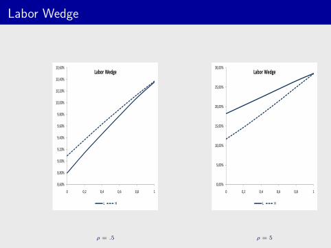
Labor Wedge

9,20%

9,40%

9,60%

9,80%

10,00%

10,20%

10,40%

10,60%

Labor Wedge

8,60%

8,80%

9,00%

9,20%

9,40%

9,60%

9,80%

10,00%

10,20%

10,40%

10,60%

0 0,2 0,4 0,6 0,8 1

Labor Wedge

L H

10,00%

15,00%

20,00%

25,00%

30,00%

Labor Wedge

0,00%

5,00%

10,00%

15,00%

20,00%

25,00%

30,00%

0 0,2 0,4 0,6 0,8 1

Labor Wedge

L H

ρ = .5 ρ = 5

Table of Contents

Introduction

The ModelEnvironmentThe Planner’s ProblemMain Results

Macro Consequences

DiscussionExtensions and CaveatsRelated Literature

Conclusion

Infinite Horizon

Link between separability and memory: ln Proposition andPure Heterogeneity case easily extend.Direction of distortion: intuition based on recursiveformulation and equivalence of relaxed problem.Lack of memory is not surprising, though hard to prove!

Steady-State?

OLG, Perpetual YouthFixed promise, w, to ’kill’ memory.

More types

Curse of DimensionalityFirst order approach?

Gov’t consumption

Results survive for Gt(zt) = gYt(z

t); Approximate ifGt(z

t) = Go + gYt(zt) for small Go.

Capital

No results, but......may relate to gov’t consumption results below.

Infinite Horizon

Link between separability and memory: ln Proposition andPure Heterogeneity case easily extend.Direction of distortion: intuition based on recursiveformulation and equivalence of relaxed problem.Lack of memory is not surprising, though hard to prove!Steady-State?

OLG, Perpetual YouthFixed promise, w, to ’kill’ memory.

More types

Curse of DimensionalityFirst order approach?

Gov’t consumption

Results survive for Gt(zt) = gYt(z

t); Approximate ifGt(z

t) = Go + gYt(zt) for small Go.

Capital

No results, but......may relate to gov’t consumption results below.

Infinite Horizon

Link between separability and memory: ln Proposition andPure Heterogeneity case easily extend.Direction of distortion: intuition based on recursiveformulation and equivalence of relaxed problem.Lack of memory is not surprising, though hard to prove!Steady-State?

OLG, Perpetual YouthFixed promise, w, to ’kill’ memory.

More types

Curse of DimensionalityFirst order approach?

Gov’t consumption

Results survive for Gt(zt) = gYt(z

t); Approximate ifGt(z

t) = Go + gYt(zt) for small Go.

Capital

No results, but......may relate to gov’t consumption results below.

Infinite Horizon

Link between separability and memory: ln Proposition andPure Heterogeneity case easily extend.Direction of distortion: intuition based on recursiveformulation and equivalence of relaxed problem.Lack of memory is not surprising, though hard to prove!Steady-State?

OLG, Perpetual YouthFixed promise, w, to ’kill’ memory.

More types

Curse of DimensionalityFirst order approach?

Gov’t consumption

Results survive for Gt(zt) = gYt(z

t); Approximate ifGt(z

t) = Go + gYt(zt) for small Go.

Capital

No results, but......may relate to gov’t consumption results below.

Infinite Horizon

Link between separability and memory: ln Proposition andPure Heterogeneity case easily extend.Direction of distortion: intuition based on recursiveformulation and equivalence of relaxed problem.Lack of memory is not surprising, though hard to prove!Steady-State?

OLG, Perpetual YouthFixed promise, w, to ’kill’ memory.

More types

Curse of DimensionalityFirst order approach?

Gov’t consumption

Results survive for Gt(zt) = gYt(z

t); Approximate ifGt(z

t) = Go + gYt(zt) for small Go.

Capital

No results, but......may relate to gov’t consumption results below.

Infinite Horizon

Link between separability and memory: ln Proposition andPure Heterogeneity case easily extend.Direction of distortion: intuition based on recursiveformulation and equivalence of relaxed problem.Lack of memory is not surprising, though hard to prove!Steady-State?

OLG, Perpetual YouthFixed promise, w, to ’kill’ memory.

More types

Curse of DimensionalityFirst order approach?

Gov’t consumption

Results survive for Gt(zt) = gYt(z

t); Approximate ifGt(z

t) = Go + gYt(zt) for small Go.

Capital

No results, but...

...may relate to gov’t consumption results below.

Infinite Horizon

Link between separability and memory: ln Proposition andPure Heterogeneity case easily extend.Direction of distortion: intuition based on recursiveformulation and equivalence of relaxed problem.Lack of memory is not surprising, though hard to prove!Steady-State?

OLG, Perpetual YouthFixed promise, w, to ’kill’ memory.

More types

Curse of DimensionalityFirst order approach?

Gov’t consumption

Results survive for Gt(zt) = gYt(z

t); Approximate ifGt(z

t) = Go + gYt(zt) for small Go.

Capital

No results, but......may relate to gov’t consumption results below.

Gov’t Consumption

g = 10%, Go = 0

24,00%

26,00%

28,00%

30,00%

32,00%

34,00%Taxes and Wedges

20,00%

22,00%

24,00%

26,00%

28,00%

30,00%

32,00%

34,00%

0 0,2 0,4 0,6 0,8 1

Taxes and Wedges

Taxes - L Taxes - H Wedge - L Wedge - H

25,00%

30,00%

35,00%

40,00%Taxes and Wedges

15,00%

20,00%

25,00%

30,00%

35,00%

40,00%

0 0,2 0,4 0,6 0,8 1

Taxes and Wedges

Taxes - L Taxes - H Wedge - L Wedge - H

ρ = .5 ρ = 5

Gov’t Consumption

g = 5%, Go > 0

10,00%

15,00%

20,00%

25,00%

30,00%

35,00%Taxes and Wedges

0,00%

5,00%

10,00%

15,00%

20,00%

25,00%

30,00%

35,00%

0 0,2 0,4 0,6 0,8 1

Taxes and Wedges

Taxes - L Taxes - H Wedge - L Wedge - H

25,00%

30,00%

35,00%

40,00%

45,00%Taxes and Wedges

15,00%

20,00%

25,00%

30,00%

35,00%

40,00%

45,00%

0 0,2 0,4 0,6 0,8 1

Taxes and Wedges

Taxes - L Taxes - H Wedge - L Wedge - H

ρ = .5 ρ = 5

Related Literature

Normative:

Kocherlakota (2005); Golosov, Tsyvinski and Werning (2007);Golosov, Troshkin and Tsyvinski(2009) - numeric examplesWerning (2007) - pure heterogeneityPhelan (1994)

Dynamic Moral Hazard; OLG; CARA; i.i.d shockShows that can be written in a recursive formAllocations display memory of aggregate shock

Demange (2008)

Positive:

Micro-consequences: Townsend (1983), Ligon, et al. (2002),Attanasio and Pavoni (2008), Ales and Maziero (2009), etc.Macro-consequences: Kocherlakota and Pistaferri (2007, 2008,2009)

Related Literature

Normative:

Kocherlakota (2005); Golosov, Tsyvinski and Werning (2007);Golosov, Troshkin and Tsyvinski(2009) - numeric examplesWerning (2007) - pure heterogeneityPhelan (1994)

Dynamic Moral Hazard; OLG; CARA; i.i.d shockShows that can be written in a recursive formAllocations display memory of aggregate shock

Demange (2008)

Positive:

Micro-consequences: Townsend (1983), Ligon, et al. (2002),Attanasio and Pavoni (2008), Ales and Maziero (2009), etc.Macro-consequences: Kocherlakota and Pistaferri (2007, 2008,2009)

Related Literature

Normative:

Kocherlakota (2005); Golosov, Tsyvinski and Werning (2007);Golosov, Troshkin and Tsyvinski(2009) - numeric examplesWerning (2007) - pure heterogeneityPhelan (1994)

Dynamic Moral Hazard; OLG; CARA; i.i.d shockShows that can be written in a recursive formAllocations display memory of aggregate shock

Demange (2008)

Positive:

Micro-consequences: Townsend (1983), Ligon, et al. (2002),Attanasio and Pavoni (2008), Ales and Maziero (2009), etc.Macro-consequences: Kocherlakota and Pistaferri (2007, 2008,2009)

Optimal Taxation

Ramsey approach (representative agent)

Finance Gov’t consumptionCannot address risk sharing and social insuranceWhy is lump sum-tax ruled out (ad hoc restriction on taxinstruments)?

Ramsey approach (heterogeneous agents)

No inter-temporal tie-ins

We: Mirrlees’ approach

Explicit tade-off between distortions today and in the future atan individual level.Focus on risk sharing and social insurance.

Optimal Taxation

Ramsey approach (representative agent)

Finance Gov’t consumptionCannot address risk sharing and social insuranceWhy is lump sum-tax ruled out (ad hoc restriction on taxinstruments)?

Ramsey approach (heterogeneous agents)

No inter-temporal tie-ins

We: Mirrlees’ approach

Explicit tade-off between distortions today and in the future atan individual level.Focus on risk sharing and social insurance.

Optimal Taxation

Ramsey approach (representative agent)

Finance Gov’t consumptionCannot address risk sharing and social insuranceWhy is lump sum-tax ruled out (ad hoc restriction on taxinstruments)?

Ramsey approach (heterogeneous agents)

No inter-temporal tie-ins

We: Mirrlees’ approach

Explicit tade-off between distortions today and in the future atan individual level.Focus on risk sharing and social insurance.

Optimal Taxation

Ramsey approach (representative agent)

Finance Gov’t consumptionCannot address risk sharing and social insuranceWhy is lump sum-tax ruled out (ad hoc restriction on taxinstruments)?

Ramsey approach (heterogeneous agents)

No inter-temporal tie-ins

We: Mirrlees’ approach

Explicit tade-off between distortions today and in the future atan individual level.Focus on risk sharing and social insurance.

How should risk be shared by society?

First best [Wilson(1968)]

MutualizationIndividual allocations only depends on current aggregate state

Constrained Efficient: No aggregate risk. [Rogerson (1985),Green (1987), Thomas and Worrall (1990), Atkeson andLucas (1992, 1995), GKT (2003), etc.]

History-dependence: long-run consequences.

Constrained Efficient: No dynamics [Demange (2008)]

Incentives and distribution of resources across groups.

Constrained Efficient: Dynamics and Aggregate Risk [Phelan(1994)]

Perpetual youth and CARA preferences ⇒ dependence onaggregate history and non-degenerate steady-state.

How should risk be shared by society?

First best [Wilson(1968)]

MutualizationIndividual allocations only depends on current aggregate state

Constrained Efficient: No aggregate risk. [Rogerson (1985),Green (1987), Thomas and Worrall (1990), Atkeson andLucas (1992, 1995), GKT (2003), etc.]

History-dependence: long-run consequences.

Constrained Efficient: No dynamics [Demange (2008)]

Incentives and distribution of resources across groups.

Constrained Efficient: Dynamics and Aggregate Risk [Phelan(1994)]

Perpetual youth and CARA preferences ⇒ dependence onaggregate history and non-degenerate steady-state.

How should risk be shared by society?

First best [Wilson(1968)]

MutualizationIndividual allocations only depends on current aggregate state

Constrained Efficient: No aggregate risk. [Rogerson (1985),Green (1987), Thomas and Worrall (1990), Atkeson andLucas (1992, 1995), GKT (2003), etc.]

History-dependence: long-run consequences.

Constrained Efficient: No dynamics [Demange (2008)]

Incentives and distribution of resources across groups.

Constrained Efficient: Dynamics and Aggregate Risk [Phelan(1994)]

Perpetual youth and CARA preferences ⇒ dependence onaggregate history and non-degenerate steady-state.

How should risk be shared by society?

First best [Wilson(1968)]

MutualizationIndividual allocations only depends on current aggregate state

Constrained Efficient: No aggregate risk. [Rogerson (1985),Green (1987), Thomas and Worrall (1990), Atkeson andLucas (1992, 1995), GKT (2003), etc.]

History-dependence: long-run consequences.

Constrained Efficient: No dynamics [Demange (2008)]

Incentives and distribution of resources across groups.

Constrained Efficient: Dynamics and Aggregate Risk [Phelan(1994)]

Perpetual youth and CARA preferences ⇒ dependence onaggregate history and non-degenerate steady-state.

How should risk be shared by society?

First best [Wilson(1968)]

MutualizationIndividual allocations only depends on current aggregate state

Constrained Efficient: No aggregate risk. [Rogerson (1985),Green (1987), Thomas and Worrall (1990), Atkeson andLucas (1992, 1995), GKT (2003), etc.]

History-dependence: long-run consequences.

Constrained Efficient: No dynamics [Demange (2008)]

Incentives and distribution of resources across groups.

Constrained Efficient: Dynamics and Aggregate Risk [Phelan(1994)]

Perpetual youth and CARA preferences ⇒ dependence onaggregate history and non-degenerate steady-state.

’Testable’ Implications

Testable Consequences of Constrained Efficiency

Idea: many ”mechanisms” can induce an allocation ⇒ focuson allocation.

Micro Consequences

Townsend (1994), Ligon, Thomas and Worrall (2002)]Ales and Maziero (2009)

Macro consequences

Asset Pricing [Kocherlakota and Pistaferri (2007,2008,2009)]

’Testable’ Implications

Testable Consequences of Constrained Efficiency

Idea: many ”mechanisms” can induce an allocation ⇒ focuson allocation.

Micro Consequences

Townsend (1994), Ligon, Thomas and Worrall (2002)]Ales and Maziero (2009)

Macro consequences

Asset Pricing [Kocherlakota and Pistaferri (2007,2008,2009)]

’Testable’ Implications

Testable Consequences of Constrained Efficiency

Idea: many ”mechanisms” can induce an allocation ⇒ focuson allocation.

Micro Consequences

Townsend (1994), Ligon, Thomas and Worrall (2002)]Ales and Maziero (2009)

Macro consequences

Asset Pricing [Kocherlakota and Pistaferri (2007,2008,2009)]

’Testable’ Implications

Testable Consequences of Constrained Efficiency

Idea: many ”mechanisms” can induce an allocation ⇒ focuson allocation.

Micro Consequences

Townsend (1994), Ligon, Thomas and Worrall (2002)]Ales and Maziero (2009)

Macro consequences

Asset Pricing [Kocherlakota and Pistaferri (2007,2008,2009)]

Table of Contents

Introduction

The ModelEnvironmentThe Planner’s ProblemMain Results

Macro Consequences

DiscussionExtensions and CaveatsRelated Literature

Conclusion

That’s all, folks!