From the SelectedWorks of Davide Ticchi

April 2007

Risk Aversion, Intertemporal Substitution, and theAggregate Investment-Uncertainty Relationship

ContactAuthor

Start Your OwnSelectedWorks

Notify Meof New Work

Available at: http://works.bepress.com/davideticchi/1

Risk aversion, intertemporal substitution, and the aggregate

investment-uncertainty relationship�

Enrico Saltariy, Davide Ticchi zx

Abstract

We analyze the role of risk aversion and intertemporal substitution in a simple dynamic

general equilibrium model of investment and savings. Our main �nding is that risk aversion

cannot by itself explain a negative relationship between aggregate investment and aggregate

uncertainty, as the e¤ect of increased uncertainty on investment also depends on the intertem-

poral elasticity of substitution. In particular, the relationship between aggregate investment and

aggregate uncertainty is positive even if agents are very risk averse, as long as the elasticity of

intertemporal substitution is low. A negative investment-uncertainty relationship requires that

the relative risk aversion and the elasticity of intertemporal substitution are both relatively high

or both relatively low. We also show that the implications of our model are consistent with the

available empirical evidence.

�Part of this paper was written while the second author was at Universitat Pompeu Fabra whose hospitality is

gratefully acknowledged. We are grateful to an anonymous referee, Antonio Cabrales, Giorgio Calcagnini, Robert

Chirinko, Annamaria Lusardi, José Marin, Enrico Pennings, seminar participants at Universitat Pompeu Fabra,

participants at the 51st International Atlantic Economic Conference and especially Janice Eberly for useful comments

and suggestions. We are heavily indebted to Antonio Ciccone for encouragements and many useful comments,

suggestions and long discussions that allowed us to improve the paper substantially. Ticchi gratefully acknowledges

�nancial support from the European Commission through the RTN grant �Specialization Versus Diversi�cation.�

Remaining errors are all ours.yDepartment of Public Economics, University of Rome �La Sapienza�, via del Castro Laurenziano 9, 00161, Roma,

Italy.zDepartment of Economics, University of Urbino, via Sa¢ 42, 61029, Urbino, Italy.xCorresponding author. Tel.: +39-0722305556; fax: +39-0722305550. E-mail address : ticchi@uniurb.it

1

JEL classi�cation: D92; E22.

Keywords: aggregate investment; aggregate savings; aggregate uncertainty; risk aversion;

intertemporal substitution.

2

1 Introduction

Economic theory has been analyzing the e¤ect of uncertainty on investment for more than forty

years. One seminal strand of the literature starts with Oi (1961), followed by Hartman (1972) and

Abel (1983). They show that, in a perfectly competitive environment, an increase in output-price

uncertainty raises the investment of a risk-neutral �rm with a constant returns to scale technology.

Intuitively, this is because constant returns to scale imply that the marginal revenue product of

capital rises more than proportionally with the output price when �rms can adjust employment

after uncertainty is resolved. Hence, the marginal revenue product of capital is convex in the output

price and, by Jensen�s inequality, greater price variability translates into a higher expected return

to capital and higher investment.

This theoretical conclusion has been contradicted by empirical research as no study has found

a positive investment-uncertainty correlation; estimates range from negative to zero. Most of the

empirical evidence is about the relationship between investment and uncertainty at the aggregate

level. Many studies are based either on country data (see Ramey and Ramey, 1995, Aizenman

and Marion, 1999, Pindyck and Solimano, 1993, Calcagnini and Saltari, 2000, Alesina and Perotti,

1996) or on highly aggregated data (see Huizinga, 1993, Ferderer, 1993a, 1993b). Only Leahy and

Whited (1996), Guiso and Parigi (1999) and Bloom, Bond and Van Reenen (2005) do empirical

work at the micro level.

Investment irreversibility has been one of the �rst elements considered by economic theory

to explain the negative e¤ect of uncertainty on investment. Bernanke (1983), McDonald and

Siegel (1986), Pindyck (1988) and Bertola (1988) show that, if the �rm cannot resell its capital

goods, then the optimal investment policy derived under reversibility, equalization of the marginal

revenue product of capital and the Jorgensonian user cost of capital (Jorgenson, 1963), does not

hold anymore. In particular, if investment is irreversible, the �rm invests only when the marginal

revenue product of capital is higher than a threshold that exceeds the Jorgensonian user cost of

capital because the �rm takes into account that the irreversibility constraint may be binding in the

3

following periods. The di¤erence between this threshold and the Jorgensonian user cost of capital

represents the value of the option of investing in the future. A higher degree of uncertainty implies

a higher threshold for investing since the value of the option is always increasing in the variance of

the stochastic variable.

The higher threshold for investing under irreversibility does not necessarily translates into lower

investment however. For this to happen, two additional conditions must be satis�ed. The �rst con-

dition, highlighted by Caballero (1991), Pindyck (1993) and Abel and Eberly (1997), is that the

marginal revenue product of capital is a decreasing function of the capital stock, i.e. that the �rm

operates under imperfect competition and/or decreasing returns to scale.1 Under perfect compe-

tition and constant returns to scale the marginal revenue product of capital is independent of the

capital stock so that current investment does not a¤ect the current and future marginal pro�tability

of capital, which implies that investment irreversibility does not change optimal investment.

The second condition required for the higher threshold for investing under irreversibility to

generate lower investment is that the current capital of the �rm is zero, which would be the case for

a �rm just getting started. This condition has been noted by Abel and Eberly (1999) who analyze

the e¤ect of irreversibility and uncertainty on the long-run capital stock (so that capital must be

positive). They show that irreversibility and uncertainty have two e¤ects on investment. One is the

increase in the user cost of capital described above that tends to reduce the capital stock compared

to the case with reversibility. But there is also a hangover e¤ect, which implies a higher capital

stock under irreversibility than under reversibility because investment irreversibility prevents the

�rm from selling capital when the marginal revenue product of capital is low. Abel and Eberly

demonstrate that neither of the two e¤ects dominates globally, so that irreversibility may increase

1A decreasing marginal revenue product of capital was necessary in the initial models of irreversible investment

under uncertainty to bound the size of the �rm given the standard assumptions of complete irreversibility and

absence of upward adjustment costs. Later contributions to this literature, as Abel and Eberly (1994, 1996, 1997),

have provided solutions to the problem of optimal investment under uncertainty in more general frameworks allowing,

for example, for �xed costs of investment, adjustment costs and partial irreversibility.

4

or decrease capital accumulation in the long-run. Higher uncertainty reinforces both the user cost

e¤ect and the hangover e¤ect and, therefore, does not help in obtaining an unambiguous result.

If the �rm has zero capital stock, the hangover e¤ect is inoperative and the user cost e¤ect is the

only e¤ect at work, which implies that an increase in uncertainty with investment irreversibility

always lower the level of capital stock compared to the case with reversibility. It is also worthwhile

noticing that the works with adjustment costs and irreversibility use partial equilibrium models

with an exogenous risk-free interest rate so that it is not clear whether the results of these papers

are about sectoral investment or aggregate investment.

To obtain a robust negative relationship between investment and uncertainty, economic theory

has taken into consideration the role of risk aversion in general equilibrium frameworks, so incor-

porating the role of savings into the model. Craine (1989) uses a model with many sectors and risk

averse households to show that an increase in exogenous risk in one sector may lead, under some

conditions, to capital being reallocated toward less risky sectors. Zeira (1990) makes a similar point

in a model where sectors di¤er in the intensity of capital and labor used. He shows that, in some

cases, higher labor cost uncertainty may shift capital from labor intensive sectors toward less risky,

capital intensive, sectors. Even though Craine and Zeira use general equilibrium models, they both

concentrate on the e¤ect of uncertainty on the reallocation of savings and investment across sectors

and in their work there is no e¤ect of uncertainty on aggregate savings/investment.2

Our goal here is instead to analyze the e¤ect of an increase in aggregate, and hence non-

diversi�able, uncertainty on aggregate equilibrium investment when agents are risk averse. There-

fore, we propose a dynamic general equilibrium model where households are risk averse and �rms

2The increase in sectoral uncertainty in the models of Craine and Zeira also leads to an increase in aggregate

uncertainty. The increase in aggregate risk does not a¤ect aggregate investment in Craine�s model, however, because

the household�s instantaneous utility function is logarithmic, which implies that aggregate savings and aggregate

investment are a �xed fraction of total output. Therefore, aggregate risk makes the time path for investment more

volatile but does not a¤ect the aggregate savings/investment decision rule. This is also the case in the overlapping

generations model of Zeira where he assumes that each individual of the young generation, independently on the

realization of the (real wage) shock, always works one unit of time, gets the real wage and saves it all.

5

are subject to aggregate exogenous shocks. This setting allows us to focus on the e¤ect of aggre-

gate uncertainty on aggregate investment instead of the e¤ect of uncertainty on the distribution

of investment across sectors as analyzed in Craine (1989) or Zeira (1990). A key feature of our

model is that we use Kreps-Porteus nonexpected utility preferences (recursive preferences) in order

to separate the role of risk aversion from that of intertemporal substitution. As is well-known, the

conventional expected utility set up with constant relative risk aversion (CRRA) preferences makes

it impossible to separate the role of these two parameters.

We show that risk aversion cannot by itself explain a negative relationship between investment

and uncertainty at the aggregate level as the e¤ect of increased uncertainty on investment also de-

pends on the intertemporal elasticity of substitution. For example, we show that if the elasticity of

intertemporal substitution is low, then an increase in aggregate uncertainty has a positive e¤ect on

aggregate investment even if risk aversion is very high. If the elasticity of intertemporal substitution

is high, however, then even small degrees of risk aversion imply a negative investment-uncertainty

relationship. Intuitively, in a dynamic framework, a high degree of risk aversion reduces the cer-

tainty equivalent of the return to capital. This does not necessarily lower investment however. The

reason is that a lower rate of return to capital generates a substitution e¤ect and an income e¤ect

a¤ecting aggregate savings and, therefore, aggregate investment in opposite directions. The substi-

tution e¤ect reduces aggregate savings and investment while the income e¤ect increases aggregate

savings/investment. The relative strength of these two e¤ects is determined by the elasticity of

intertemporal substitution. If the elasticity of substitution is lower than unity, the income ef-

fect dominates and the equilibrium investment increases as a result of increased uncertainty. The

opposite happens if the elasticity of substitution is greater than unity.

We characterize the aggregate investment-uncertainty relationship for all possible parameter

values of the Kreps-Porteus nonexpected utility preferences as well as for the standard CRRA ex-

pected utility preferences (which are a special case of the recursive preferences). We show that the

relationship is generally ambiguous and depends on the value of technological and preference para-

meters. A negative relationship between aggregate investment and aggregate uncertainty requires

6

that the relative risk aversion and the elasticity of intertemporal substitution are both relatively

high or both relatively low. If this is not the case, the relationship is positive. With CRRA prefer-

ences the region of the parameter values where the relationship is negative is generally small and

the fact that the elasticity of intertemporal substitution is the inverse of the coe¢ cient of relative

risk aversion implies that high values of risk aversion always lead to a positive correlation between

aggregate investment and aggregate uncertainty.3 We also study the investment-uncertainty re-

lationship implied by empirically plausible values of the relative risk aversion and the elasticity

of intertemporal substitution and �nd that the wide range of estimates available in the literature

implies that our model is compatible with a negative, positive, or no relationship between aggregate

investment and aggregate uncertainty.

Our results therefore suggest that risk aversion, as well as irreversibility, is not enough to

generate a theoretically robust negative investment-uncertainty relationship. Indeed, even though

increased uncertainty in one sector may reduce investment in that sector, the same needs not to be

true at the aggregate level as the e¤ect of uncertainty on aggregate savings/investment is di¤erent

than the e¤ect of uncertainty on the allocation of savings and investment across sectors.

The paper is organized as follows. Section 2 presents the model with recursive preferences and

analyzes the relationship between aggregate uncertainty and aggregate investment for all possible

values of the coe¢ cients of relative risk aversion and intertemporal substitution elasticity. Section

3 relates the implications of the model to the evidence on the investment-uncertainty relationship.

Section 4 concludes. Detailed proofs of the main propositions and an extension of the baseline

model can be found in the Appendix.

3 It is immediate that this result can be understood only using recursive preferences that allows us to separate the

role of risk aversion from the role of intertemporal substitution.

7

2 The model

We assume that the technology of the competitive �rm is described by the following constant

returns to scale Cobb-Douglas production function

Yt = BtK1��t L�t (1)

whereKt is the stock of capital, Lt is the amount of labor employed andBt = Be#t is a multiplicative

shock to the production function. We assume that B is a constant and #t is an identically and

independently distributed normal random variable with variance �2 and mean # � 12�

2.4 This

parametrization implies that the expected value of the multiplicative shock is a function of # only

(does not depend on �2) and that the variance of the multiplicative shock is increasing in �2.

Hence, an increase in �2 increases the variance of the multiplicative shock (and hence the degree

of uncertainty) without a¤ecting its expected value. The parameters # and �2 are assumed to be

constant over time.5 The i:i:d: assumption is crucial for the derivation of the investment function,

and the log-normality assumption permits us to derive the e¤ect of uncertainty on investment

analytically.6

We assume that the �rm can adjust the amount of labor employed in each period but that the

capital stock is decided one period in advance. In each period, the �rm �rst observes the realization

of the shock and then adjust the amount of labor. Choosing output as the numeraire, the �rm�s

operating pro�t (i.e. revenues minus the cost of variable inputs) is therefore equal to

4 In this Section, we only discuss the e¤ect of technological uncertainty on aggregate investment. In Appendix D,

we extend this framework to analyze also the e¤ect of preference shocks.5As most models in this literature, we make a comparative static analysis and do not allow for time-varying

uncertainty. See, for example, Guo, Miao and Morellec (2005) for a contribution that analyzes the dynamic of

investment when the growth rate and volatility of the marginal revenue product of capital are subject to discrete

regime shifts at random times.6The i:i:d: assumption is also made in Craine (1989) and Zeira (1990). The investment function and the e¤ect of

uncertainty on investment cannot be derived analytically when the shock is subject to a trend or displays persistence.

In this case it is necessary to use numerical solution methods.

8

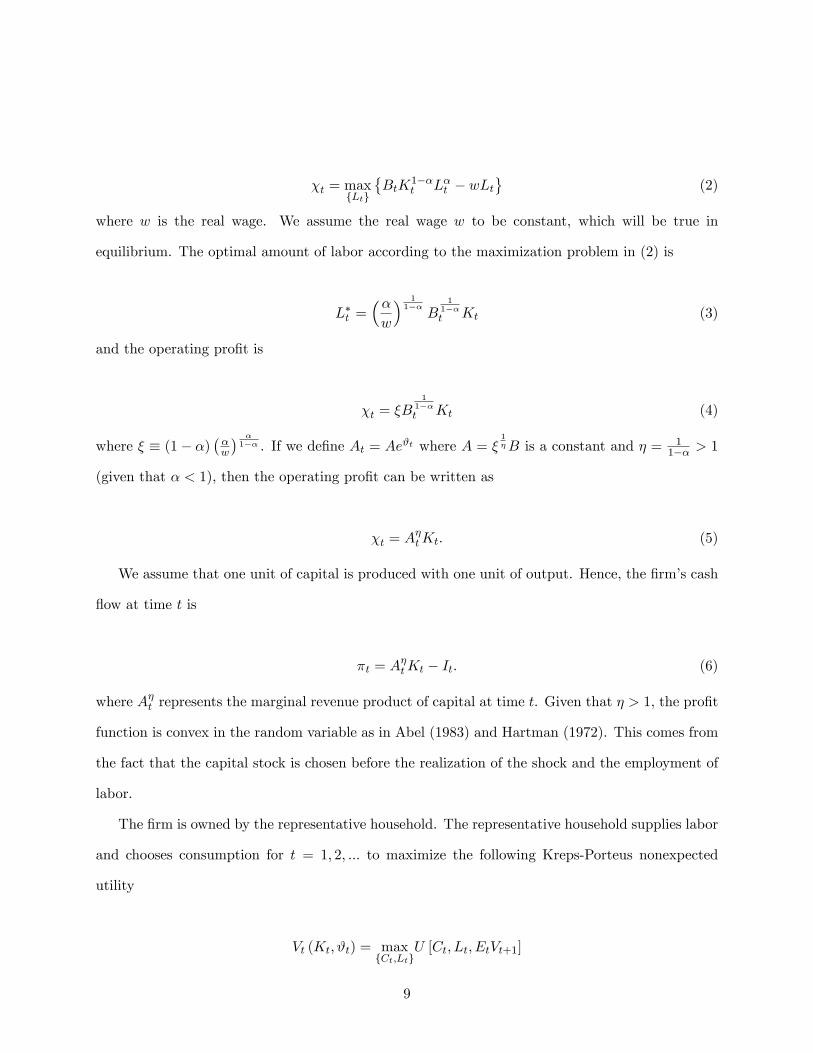
�t = maxfLtg

�BtK

1��t L�t � wLt

(2)

where w is the real wage. We assume the real wage w to be constant, which will be true in

equilibrium. The optimal amount of labor according to the maximization problem in (2) is

L�t =��w

� 11��

B1

1��t Kt (3)

and the operating pro�t is

�t = �B1

1��t Kt (4)

where � � (1� �)��w

� �1�� . If we de�ne At = Ae#t where A = �

1�B is a constant and � = 1

1�� > 1

(given that � < 1), then the operating pro�t can be written as

�t = A�tKt: (5)

We assume that one unit of capital is produced with one unit of output. Hence, the �rm�s cash

�ow at time t is

�t = A�tKt � It: (6)

where A�t represents the marginal revenue product of capital at time t. Given that � > 1, the pro�t

function is convex in the random variable as in Abel (1983) and Hartman (1972). This comes from

the fact that the capital stock is chosen before the realization of the shock and the employment of

labor.

The �rm is owned by the representative household. The representative household supplies labor

and chooses consumption for t = 1; 2; ::: to maximize the following Kreps-Porteus nonexpected

utility

Vt (Kt; #t) = maxfCt;Ltg

U [Ct; Lt; EtVt+1]

9

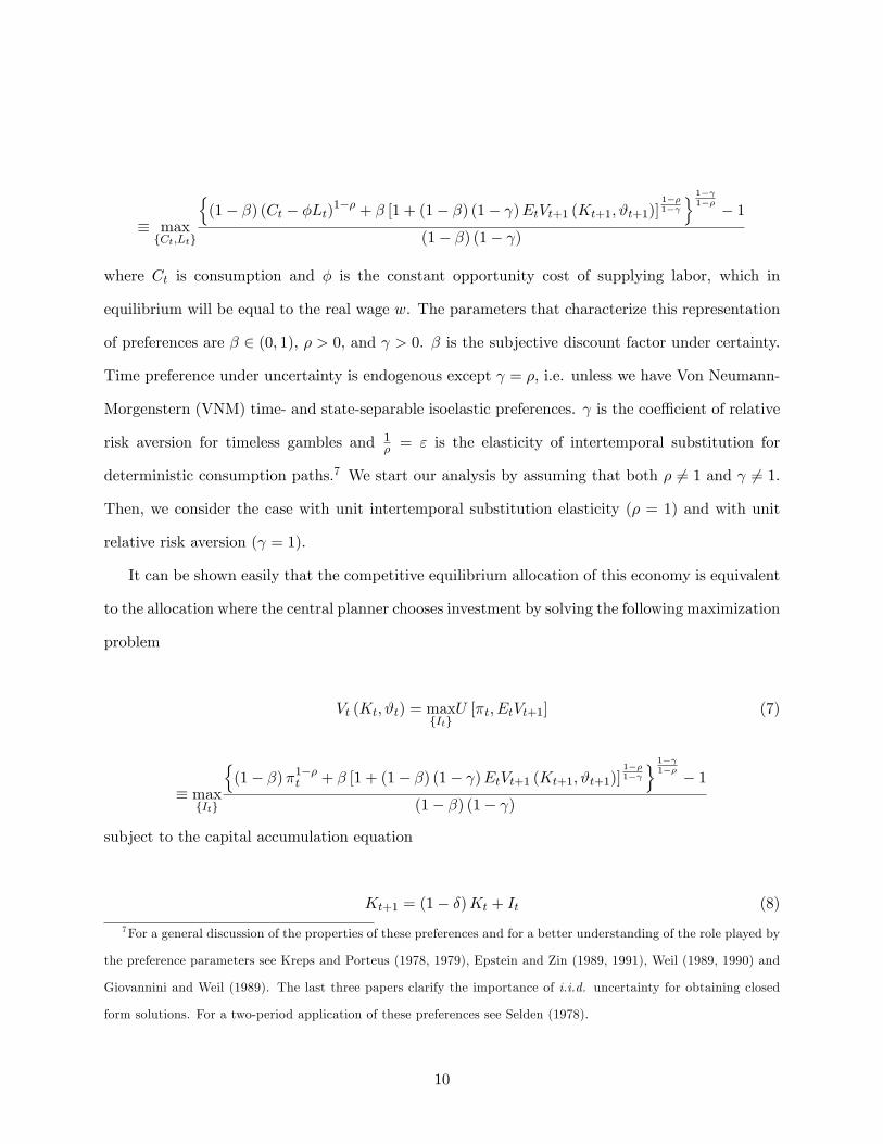
� maxfCt;Ltg

n(1� �) (Ct � �Lt)1�� + � [1 + (1� �) (1� )EtVt+1 (Kt+1; #t+1)]

1��1� o 1� 1�� � 1

(1� �) (1� )

where Ct is consumption and � is the constant opportunity cost of supplying labor, which in

equilibrium will be equal to the real wage w. The parameters that characterize this representation

of preferences are � 2 (0; 1), � > 0, and > 0. � is the subjective discount factor under certainty.

Time preference under uncertainty is endogenous except = �, i.e. unless we have Von Neumann-

Morgenstern (VNM) time- and state-separable isoelastic preferences. is the coe¢ cient of relative

risk aversion for timeless gambles and 1� = " is the elasticity of intertemporal substitution for

deterministic consumption paths.7 We start our analysis by assuming that both � 6= 1 and 6= 1.

Then, we consider the case with unit intertemporal substitution elasticity (� = 1) and with unit

relative risk aversion ( = 1).

It can be shown easily that the competitive equilibrium allocation of this economy is equivalent

to the allocation where the central planner chooses investment by solving the following maximization

problem

Vt (Kt; #t) = maxfItg

U [�t; EtVt+1] (7)

� maxfItg

n(1� �)�1��t + � [1 + (1� �) (1� )EtVt+1 (Kt+1; #t+1)]

1��1� o 1� 1�� � 1

(1� �) (1� )

subject to the capital accumulation equation

Kt+1 = (1� �)Kt + It (8)

7For a general discussion of the properties of these preferences and for a better understanding of the role played by

the preference parameters see Kreps and Porteus (1978, 1979), Epstein and Zin (1989, 1991), Weil (1989, 1990) and

Giovannini and Weil (1989). The last three papers clarify the importance of i.i.d. uncertainty for obtaining closed

form solutions. For a two-period application of these preferences see Selden (1978).

10

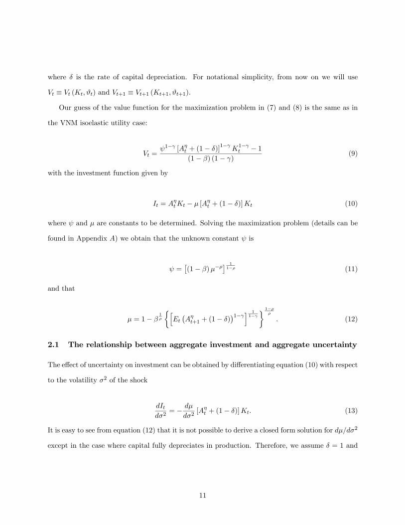
where � is the rate of capital depreciation. For notational simplicity, from now on we will use

Vt � Vt (Kt; #t) and Vt+1 � Vt+1 (Kt+1; #t+1).

Our guess of the value function for the maximization problem in (7) and (8) is the same as in

the VNM isoelastic utility case:

Vt = 1� [A�t + (1� �)]

1� K1� t � 1

(1� �) (1� ) (9)

with the investment function given by

It = A�tKt � � [A�t + (1� �)]Kt (10)

where and � are constants to be determined. Solving the maximization problem (details can be

found in Appendix A) we obtain that the unknown constant is

=�(1� �)���

� 11�� (11)

and that

� = 1� �1�

�hEt�A�t+1 + (1� �)

�1� i 11� � 1��

�

: (12)

2.1 The relationship between aggregate investment and aggregate uncertainty

The e¤ect of uncertainty on investment can be obtained by di¤erentiating equation (10) with respect

to the volatility �2 of the shock

dItd�2

= � d�

d�2[A�t + (1� �)]Kt: (13)

It is easy to see from equation (12) that it is not possible to derive a closed form solution for d�=d�2

except in the case where capital fully depreciates in production. Therefore, we assume � = 1 and

11

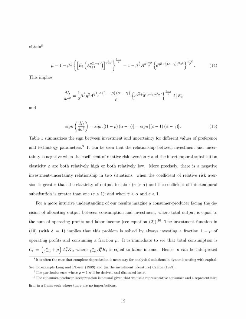
obtain8

� = 1� �1�

�hEt

�A�(1� )t+1

�i 11� � 1��

�

= 1� �1�A

� 1���

ne�#+

12(�� )�2�2

o 1���: (14)

This implies

dItd�2

=1

2�1� �2A

� 1���(1� �) (�� )

�

ne�#+

12(�� )�2�2

o 1���A�tKt

and

sign

�dItd�2

�= sign [(1� �) (�� )] = sign [("� 1) (�� )] : (15)

Table 1 summarizes the sign between investment and uncertainty for di¤erent values of preference

and technology parameters.9 It can be seen that the relationship between investment and uncer-

tainty is negative when the coe¢ cient of relative risk aversion and the intertemporal substitution

elasticity " are both relatively high or both relatively low. More precisely, there is a negative

investment-uncertainty relationship in two situations: when the coe¢ cient of relative risk aver-

sion is greater than the elasticity of output to labor ( > �) and the coe¢ cient of intertemporal

substitution is greater than one (" > 1); and when < � and " < 1.

For a more intuitive understanding of our results imagine a consumer-producer facing the de-

cision of allocating output between consumption and investment, where total output is equal to

the sum of operating pro�ts and labor income (see equation (2)).10 The investment function in

(10) (with � = 1) implies that this problem is solved by always investing a fraction 1 � � of

operating pro�ts and consuming a fraction �. It is immediate to see that total consumption is

Ct =�

�1�� + �

�A�tKt, where �

1��A�tKt is equal to labor income. Hence, � can be interpreted

8 It is often the case that complete depreciation is necessary for analytical solutions in dynamic setting with capital.

See for example Long and Plosser (1983) and (in the investment literature) Craine (1989).9The particular case where � = 1 will be derived and discussed later.10The consumer-producer interpretation is natural given that we use a representative consumer and a representative

�rm in a framework where there are no imperfections.

12

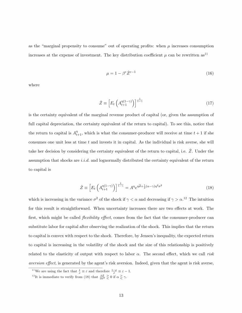
as the �marginal propensity to consume�out of operating pro�ts: when � increases consumption

increases at the expense of investment. The key distribution coe¢ cient � can be rewritten as11

� = 1� �" �Z"�1 (16)

where

�Z �hEt

�A�(1� )t+1

�i 11�

(17)

is the certainty equivalent of the marginal revenue product of capital (or, given the assumption of

full capital depreciation, the certainty equivalent of the return to capital). To see this, notice that

the return to capital is A�t+1, which is what the consumer-producer will receive at time t+ 1 if she

consumes one unit less at time t and invests it in capital. As the individual is risk averse, she will

take her decision by considering the certainty equivalent of the return to capital, i.e. �Z. Under the

assumption that shocks are i:i:d: and lognormally distributed the certainty equivalent of the return

to capital is

�Z �hEt

�A�(1� )t+1

�i 11�

= A�e�#+12(�� )�2�2 (18)

which is increasing in the variance �2 of the shock if < � and decreasing if > �.12 The intuition

for this result is straightforward. When uncertainty increases there are two e¤ects at work. The

�rst, which might be called �exibility e¤ect, comes from the fact that the consumer-producer can

substitute labor for capital after observing the realization of the shock. This implies that the return

to capital is convex with respect to the shock. Therefore, by Jensen�s inequality, the expected return

to capital is increasing in the volatility of the shock and the size of this relationship is positively

related to the elasticity of output with respect to labor �. The second e¤ect, which we call risk

aversion e¤ect, is generated by the agent�s risk aversion. Indeed, given that the agent is risk averse,

11We are using the fact that 1�� " and therefore 1��

�� "� 1.

12 It is immediate to verify from (18) that @ �Z@�2

R 0 if � R .

13

she does not take her decisions considering the expected return to capital but the correspondent

certainty equivalent, which is negatively related to the riskiness of the return, here represented by

the variance of the shock. It is clear that the magnitude of this e¤ect increases with the degree of

risk aversion of the consumer-producer. The �nal e¤ect of uncertainty on the certainty equivalent

of the return to capital �Z depends on which of the two e¤ects is bigger. If risk aversion is su¢ ciently

small ( < � < 1) for the �exibility e¤ect to prevail over the risk aversion e¤ect, then �Z will be

increasing in the variance �2 of the shock. If risk aversion is big enough ( > �), then the risk

aversion e¤ect is stronger than the �exibility e¤ect and �Z will be decreasing in the shock�s volatility.

Hence, an increase in uncertainty changes the certainty equivalent of the return to capital.

This gives rise to an income and a substitution e¤ect a¤ecting aggregate investment in opposite

directions. The �nal e¤ect of aggregate uncertainty on aggregate investment will depend on the

magnitude of the elasticity of intertemporal substitution because " determines the relative strength

of income and substitution e¤ects. To see how things work, let us assume that the coe¢ cient of

relative risk aversion is lower than the elasticity of output with respect to labor ( < � < 1) so that

an increase in uncertainty produces an increase in the certainty equivalent of the return to capital �Z.

The substitution e¤ect induces the consumer-producer to save and invest more (and consequently

consume less) because capital is more productive. The income e¤ect (due to the fact that a higher

productivity of capital makes the consumer-producer richer) implies higher consumption and lower

savings and investment. If the elasticity of intertemporal substitution is greater than one (" > 1),

then the substitution e¤ect prevails over the income e¤ect and investment will increase. This is

immediate from equation (16): an increase in �Z leads to a decrease in � whenever " > 1. If the

elasticity of intertemporal substitution is less than one (" < 1), then the income e¤ect more than

balances the substitution e¤ect. This leads the agent to consume more and invest less. Equation

(16) shows how an increase in �Z implies an increase in � whenever " < 1.

A similar argument applies to the situation where the coe¢ cient of relative risk aversion is higher

than the elasticity of output to labor ( > �).13 In this case an increase in uncertainty reduces the

13Even though the discussion on the empirically plausible values of the parameters is presented in the next Section,

14

certainty equivalent of the return to capital. The substitution e¤ect induces the consumer-producer

to invest less because the return to capital (in certainty equivalent terms) is lower. On the other

hand, the income e¤ect increases investment by pushing down the individual�s consumption because

the lower productivity of capital makes the consumer-producer poorer. Again, if the elasticity of

intertemporal substitution is greater than one (" > 1), then the substitution e¤ect more than

balances the income e¤ect and investment decreases, while the opposite happens when " < 1.14

2.2 Two special cases: unit elasticity of intertemporal substitution and CRRA

Let us now consider the case with unit elasticity of intertemporal substitution (� = 1). The

maximization problem is now given by equation15

Vt = maxfItg

n�(1��)(1� )t (EtVt+1)

�o:

By making the same guess and performing the same steps of the previous maximization problem,

we obtain that investment is still given by equation (10) but that

it is worthy to notice since now that > � is the relevant region of the parameter space given that � < 1.14At this point it may be useful to clarify the di¤erence between our model and the standard model of intertemporal

consumption choice. An increase in the volatility of the future income �ows always increases savings in the standard

model as it generates a precautionary savings e¤ect (i.e. a negative income e¤ect) given the widespread assumptions

of convex marginal utility (see Leland, 1968) and existence of a risk-free asset. So one may think that in our model an

increase in uncertainty would increase savings and investment for the same reason. But this is not the case because

in our model uncertainty is in the return of the asset used to transfer wealth over time. In the terminology of Sandmo

(1970), in our model there is a �capital risk� instead of the �income risk� of the standard model. An increase in

uncertainty of the return to capital (assuming that > � so that the �exibility e¤ect is dominated by the risk aversion

e¤ect) generates an income e¤ect (precautionary savings e¤ect) also in our model because it raises the probability of

low levels of consumption in the following period. This leads the agents to insure themselves by consuming less today

so increasing the current level of savings. However, in our model there is also a substitution e¤ect as the agents try

to reduce their exposure to risk by increasing current consumption and reducing savings (given that uncertainty is

on the savings vehicle). The magnitude of the intertemporal elasticity of substitution de�nes the relative strength of

the income and substitution e¤ects.15See Appendix B for the mathematical details.

15

� = 1� �:

It is immediate that in this case investment is not a¤ected by uncertainty for any given value of

the coe¢ cient of relative risk aversion: this result holds even with partial depreciation of capital.

This is because, independently from what happens to the certainty equivalent of the return to

capital (i.e. Q �), income and substitution e¤ects exactly o¤set each other (as in the logarithmic

preference case).16

Another particular case is the one corresponding to the CRRA preferences: these preferences

are obtained when the coe¢ cient of relative risk aversion is equal to the inverse of the intertemporal

substitution elasticity ( = � � 1" ). Clearly, the investment function is still given by equation (10)

with � (see equation (12)) equal to

� = 1� �1

�hEt�A�t+1 + (1� �)

�1� i 11� � 1�

:

As before, to get a closed form solution for the e¤ect of uncertainty on investment it is necessary

to assume complete depreciation of capital (� = 1). In this case

� = 1� �1

�hEt

�A�(1� )t+1

�i 11� � 1�

= 1� �1 A

� 1�

ne�#+

12(�� )�2�2

o 1�

and

dItd�2

=1

2�1 �2

(1� ) (�� )

ne�#+

12(�� )�2�2

o 1� A�tKt

which means that

sign

�dItd�2

�= sign [(1� ) (�� )] :

16As we already said, logarithmic preferences correspond to the case where = � = 1. The maximization problem

when the coe¢ cient of relative risk aversion is equal to one ( = 1) can be found in Appendix C. The results and

the interpretation correspond to the case discussed above where > �, given that � is always lower than one.

16

Table 2 summarizes the relationship between aggregate investment and aggregate uncertainty

for di¤erent values of the relative risk aversion coe¢ cient. It is easy to see that the e¤ect of uncer-

tainty on investment is generally positive except when � < < 1.17 This is because with CRRA

preferences the coe¢ cient of relative risk aversion is the inverse of the elasticity of intertempo-

ral substitution ( = 1="), which implies that only two main situations are possible. First, the

coe¢ cient of relative risk aversion is less than one ( < 1): this implies that the elasticity of in-

tertemporal substitution is greater than one (" > 1). If � < < 1, then greater uncertainty reduces

the certainty equivalent of the return to capital �Z. As " > 1, the substitution e¤ect prevails over

the income e¤ect, leading to lower investment. When risk aversion is small enough (0 < < � < 1),

then more uncertainty increases the certainty equivalent of the return to capital �Z and this raises

investment.18 The second situation is when the coe¢ cient of relative risk aversion is greater than

one ( > 1). Hence, it is greater than the elasticity of output with respect to labor � and the

elasticity of intertemporal substitution is less than one (" < 1). In this case greater uncertainty

decreases the certainty equivalent of the expected return to capital �Z (as > �). The fact that the

elasticity of intertemporal substitution is less than one implies that the income e¤ect more than

balances the substitution e¤ect, and this implies higher investment.19

2.3 The investment-uncertainty relationship under partial capital depreciation

In the analysis developed above we have assumed that capital fully depreciates in production

(� = 1) in order to obtain a closed form solution for the relationship between aggregate investment

and aggregate uncertainty. We now relax this assumption and analyze what happens when the

17Moreover, what seems to be surprising is that the investment-uncertainty relationship is positive when agents are

very risk averse ( > 1).18 It is immediate that if = � then volatility has no e¤ect on �Z (because the �exibility e¤ect and the risk aversion

e¤ect exactly compensate each other) and therefore it does not a¤ect investment.19 If the coe¢ cient of relative risk aversion is equal to one (and to the elasticity of intertemporal substitution)

then the utility function is logarithmic. In this case uncertainty has no e¤ect on investment because the income and

substitution e¤ect exactly o¤set each other (given that " = 1).

17

depreciation of capital is only partial (� < 1) using numerical simulation methods. Similarly to the

case of � = 1, the determination of the aggregate investment-uncertainty relationship requires the

analysis of the behavior of the distribution parameter � with respect to �2.20 This parameter is

still given by (16) but the certainty equivalent of the return to capital is now equal to

�Z �hEt�A�t+1 + (1� �)

�1� i 11�

: (19)

This implies that removing the assumption of full capital depreciation may have an e¤ect only

on the certainty equivalent of the return to capital and therefore on the relative strength of the

�exibility e¤ect and the risk aversion e¤ect. Indeed, it is immediate to verify from (16) that once

we have determined the e¤ect of uncertainty (represented by �2) on �Z, the income and substitution

e¤ects work as usual. If the elasticity of intertemporal substitution is greater than one (" > 1),

the substitution e¤ect prevails over the income e¤ect and vice versa. This means that we can

concentrate our analysis on the e¤ect of uncertainty on the certainty equivalent of the return to

capital �Z.

In the previous section we have seen that �Z is increasing in �2 if < � and decreasing if > �

when capital fully depreciates in production (� = 1). Given that it is not possible to obtain a closed

form solution for the derivative of �Z with respect to �2 when � is lower than one, we have made a

numerical analysis. We have found that for each value of the capital depreciation �, there exists a

threshold value of the coe¢ cient of relative risk aversion � such that the certainty equivalent of the

return to capital �Z is increasing in �2 if < � and decreasing if > �.21 Figure 1 presents three

examples on the relationship between the derivative of �Z with respect to �2 and the coe¢ cient of

relative risk aversion for the following parameterization: � = 0:3, # = 0:2, A = 1, � = 0:67, and

for � = 0, 0:5 and 1. The results con�rm that @ �Z@�2

is positive if < �, it is zero at � and then

becomes negative for > �. The �gure shows the derivative of �Z with respect to �2 for only three

20This is apparent from an inspection of the derivative of the investment function with respect to �2 in (13).21 In words, the threshold value of the coe¢ cient of relative risk aversion that de�nes the behavior of �Z with respect

to uncertainty is � when � = 1 and � when � < 1. The properties of � are discussed below.

18

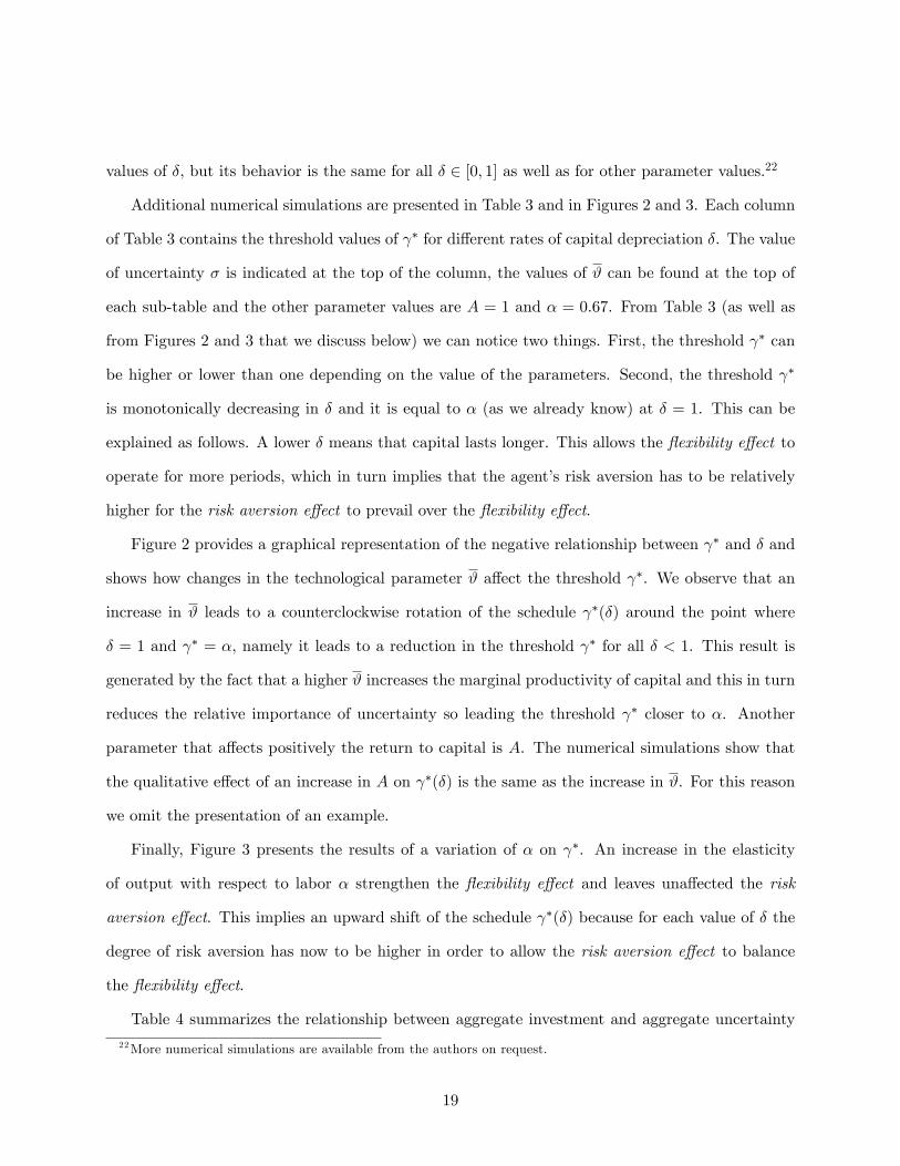
values of �, but its behavior is the same for all � 2 [0; 1] as well as for other parameter values.22

Additional numerical simulations are presented in Table 3 and in Figures 2 and 3. Each column

of Table 3 contains the threshold values of � for di¤erent rates of capital depreciation �. The value

of uncertainty � is indicated at the top of the column, the values of # can be found at the top of

each sub-table and the other parameter values are A = 1 and � = 0:67. From Table 3 (as well as

from Figures 2 and 3 that we discuss below) we can notice two things. First, the threshold � can

be higher or lower than one depending on the value of the parameters. Second, the threshold �

is monotonically decreasing in � and it is equal to � (as we already know) at � = 1. This can be

explained as follows. A lower � means that capital lasts longer. This allows the �exibility e¤ect to

operate for more periods, which in turn implies that the agent�s risk aversion has to be relatively

higher for the risk aversion e¤ect to prevail over the �exibility e¤ect.

Figure 2 provides a graphical representation of the negative relationship between � and � and

shows how changes in the technological parameter # a¤ect the threshold �. We observe that an

increase in # leads to a counterclockwise rotation of the schedule �(�) around the point where

� = 1 and � = �, namely it leads to a reduction in the threshold � for all � < 1. This result is

generated by the fact that a higher # increases the marginal productivity of capital and this in turn

reduces the relative importance of uncertainty so leading the threshold � closer to �. Another

parameter that a¤ects positively the return to capital is A. The numerical simulations show that

the qualitative e¤ect of an increase in A on �(�) is the same as the increase in #. For this reason

we omit the presentation of an example.

Finally, Figure 3 presents the results of a variation of � on �. An increase in the elasticity

of output with respect to labor � strengthen the �exibility e¤ect and leaves una¤ected the risk

aversion e¤ect. This implies an upward shift of the schedule �(�) because for each value of � the

degree of risk aversion has now to be higher in order to allow the risk aversion e¤ect to balance

the �exibility e¤ect.

Table 4 summarizes the relationship between aggregate investment and aggregate uncertainty

22More numerical simulations are available from the authors on request.

19

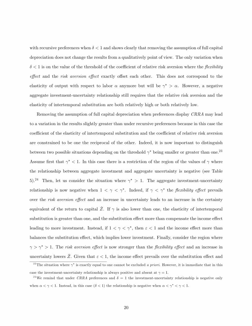
with recursive preferences when � < 1 and shows clearly that removing the assumption of full capital

depreciation does not change the results from a qualitatively point of view. The only variation when

� < 1 is on the value of the threshold of the coe¢ cient of relative risk aversion where the �exibility

e¤ect and the risk aversion e¤ect exactly o¤set each other. This does not correspond to the

elasticity of output with respect to labor � anymore but will be � > �. However, a negative

aggregate investment-uncertainty relationship still requires that the relative risk aversion and the

elasticity of intertemporal substitution are both relatively high or both relatively low.

Removing the assumption of full capital depreciation when preferences display CRRA may lead

to a variation in the results slightly greater than under recursive preferences because in this case the

coe¢ cient of the elasticity of intertemporal substitution and the coe¢ cient of relative risk aversion

are constrained to be one the reciprocal of the other. Indeed, it is now important to distinguish

between two possible situations depending on the threshold � being smaller or greater than one.23

Assume �rst that � < 1. In this case there is a restriction of the region of the values of where

the relationship between aggregate investment and aggregate uncertainty is negative (see Table

5).24 Then, let us consider the situation where � > 1. The aggregate investment-uncertainty

relationship is now negative when 1 < < �. Indeed, if < � the �exibility e¤ect prevails

over the risk aversion e¤ect and an increase in uncertainty leads to an increase in the certainty

equivalent of the return to capital �Z. If is also lower than one, the elasticity of intertemporal

substitution is greater than one, and the substitution e¤ect more than compensate the income e¤ect

leading to more investment. Instead, if 1 < < �, then " < 1 and the income e¤ect more than

balances the substitution e¤ect, which implies lower investment. Finally, consider the region where

> � > 1. The risk aversion e¤ect is now stronger than the �exibility e¤ect and an increase in

uncertainty lowers �Z. Given that " < 1, the income e¤ect prevails over the substitution e¤ect and

23The situation where � is exactly equal to one cannot be excluded a priori. However, it is immediate that in this

case the investment-uncertainty relationship is always positive and absent at = 1.24We remind that under CRRA preferences and � = 1 the investment-uncertainty relationship is negative only

when � < < 1. Instead, in this case (� < 1) the relationship is negative when � < � < < 1.

20

investment increases. These results are presented in Table 6.25

From this analysis we conclude that under CRRA preferences relaxing the assumption of full

capital depreciation does not change the main features of the aggregate investment-uncertainty

relationship, namely that the region of the values of where this relationship is negative is close

to one, and that a su¢ ciently high level of risk aversion always leads aggregate investment and

aggregate uncertainty to be a positively related.

3 Discussion and empirical evidence

The aim of our work is to analyze the relationship between aggregate uncertainty and aggregate

investment. To this purpose, in the previous Section we have proposed a closed economy model

with only one asset (the representative �rm) and we have analyzed the e¤ects of an increase in the

volatility of the returns of this asset on savings/investment. In our model we have assumed that

there is no alternative asset where the agents can invest their savings, like for example an external

asset, for the following reasons. First, we are interested in analyzing the response of aggregate

savings/investment to a systemic increase in risk, namely to a risk that cannot be eliminated by

households with a portfolio reallocation. In other words, we want to study the variation of aggregate

savings/investment when all activities in the economy become riskier and not what happens to

the investment in one sector when uncertainty in this sector (or other sectors) increases as the

analysis of these reallocation e¤ects is already well understood in Craine (1989) and Zeira (1990).

Second, there are many situations where the access to external capital markets is available only to

sophisticated investors while ordinary savers do not have this opportunity as a practical matter.

We now turn to the empirical evidence on the investment-uncertainty relationship. Even though

the theory of investment under uncertainty has been developed with reference to the single �rm,

most of the evidence about the investment-uncertainty relationship is based on aggregate data.

25 It is clear that uncertainty does not a¤ect investment if = 1 or = � because in the �rst case " = 1 and the

income and substitution e¤ects exactly compensate each other and in the second one the �exibility e¤ect and the risk

aversion e¤ect have the same strength.

21

We know of only three papers, Leahy and Whited (1996), Guiso and Parigi (1999) and Bloom,

Bond and Van Reenen (2005), where the investment-uncertainty relationship is investigated using

micro data. Cross-country and time series studies using aggregate data are instead quite abundant.

Ramey and Ramey (1995) in a sample of 92 countries (from 1960-1985) and 24 OECD countries

(from 1950-1988) �nd that countries with higher volatility (of per capita annual growth rates or of

the innovations to growth) have lower growth but their evidence suggests that investment is not

an empirically important conduit between volatility and growth. Indeed, volatility appears to have

a negative relationship with investment and is signi�cant at the 10-percent level in the 92 country

sample, but not in the case of the OECD sample. However, once the other standard control variables

are included in the investment equation (see Levine and Renelt, 1992) the e¤ect of uncertainty on

investment is positive for the 92-country sample and negative in the OECD sample, but it is no

longer signi�cant in both cases. Thus, these authors �nd little evidence that the investment share

of GDP is linked to volatility.

Aizenman and Marion (1999) investigate the investment-uncertainty relationship using a sample

of 46 developing countries over the period 1970-1992. They �nd a statistically signi�cant negative

correlation between various volatility measures (two internal and one external) and private invest-

ment even when standard control variables are added. They also �nd that there is no aggregate

investment-uncertainty correlation due to a positive relationship between uncertainty and public

investment spending.

Pindyck and Solimano (1993) use cross section and time series data for a set of developing and

industrialized countries and �nd that the volatility of the marginal pro�tability of capital (which

they use as summary measure of uncertainty) a¤ects aggregate investment negatively but that the

size of this e¤ect is moderate (overall larger for developing countries). A detailed analysis of the

shortcomings of their measure of uncertainty and their results can be found in Eberly (1993).

Calcagnini and Saltari (2000), using data on the Italian economy for the period 1971-1995, �nd

that changes in the level of volatility of expected demand have a negative impact on aggregate

22

investment.26

Alesina and Perotti (1996) analyze a sample of 71 countries for the period 1960-1985 and

�nd a negative correlation between indices of political and social instability, taken as proxies of

uncertainty, and aggregate investment. A similar result is obtained by Barro (1991) who �nds that

measures of political instability and aggregate investment are negatively related for 98 countries in

the period 1960-1985. These results are consistent with the �nding of several other papers like, for

example, Aizenman and Marion (1993).

All the studies cited so far consider investment at the country level. There are also empirical

studies that use important parts of aggregate investment and that can therefore provide insightful

information on the aggregate investment-uncertainty relationship. For example, Huizinga (1993)

provides evidence that in�ation uncertainty reduces aggregate investment using U.S. manufactur-

ing data over the period 1954-1989. Ferderer (1993a) explores the empirical relationship between

uncertainty and real gross expenditures on producers� durable equipment and the real value of

contracts and orders for new plant and equipment using U.S. data from 1969 to 1989. He measures

uncertainty about interest rates and other macroeconomic variables using the risk premium em-

bedded in the term structure and �nds a signi�cant negative impact of uncertainty on investment.

Ferderer (1993b) obtains the same result with a di¤erent sample and methodology.

The aggregate investment-uncertainty relationship predicted by our model depends crucially on

the coe¢ cient of relative risk aversion and the elasticity of intertemporal substitution. Two studies

that estimate these two parameters separately are Attanasio and Weber (1989) and Epstein and

Zin (1991). Attanasio and Weber �nd an elasticity of intertemporal substitution between 1.946 and

2.247 and a coe¢ cient of relative risk aversion ranging from 5.1 to 29.9. For these values, our model

predicts a negative relationship between aggregate investment and aggregate uncertainty even when

we consider the case of partial capital depreciation given that the values of the coe¢ cient of relative

26 In the paper the investment rate refers to the whole economy while demand variables refer to industrial �rms.

More precisely, the authors used monthly survey data about Italian industrial �rms� expectations regarding the

growth in orders over the 3-4 months to come.

23

risk aversion obtained by Attanasio and Weber are pretty high. Epstein and Zin �nd a coe¢ cient

of relative risk aversion close to one and a coe¢ cient of intertemporal substitution between 0.2 and

0.87. These parameter values would lead to a positive correlation between aggregate investment and

aggregate uncertainty in the baseline version of our model (i.e. with complete capital depreciation).

If we consider the model with partial capital depreciation (which is clearly more realistic), the

threshold � is higher than the elasticity of output with respect to labor (� = 0:67) and it can also

be higher than one. This means that with the Epstein and Zin�s estimates of " and our model

is compatible with both a positive or a negative (or even absent) relationship between aggregate

investment and aggregate uncertainty.27

Most empirical work estimates the key parameters of our model using an expected utility frame-

work with a CRRA utility function (which implies that the coe¢ cient of relative risk aversion and

the elasticity of intertemporal substitution are linked). Hansen and Singleton (1983), Eichennbaum,

Hansen, and Singleton (1988) and Gourinchas and Parker (2002) estimate a range of values for the

constant relative risk aversion parameter that is consistent with both a negative and a positive ag-

gregate investment-uncertainty relationship in our model (more or less independently on the degree

of capital depreciation that we may consider).28 Hansen and Singleton (1982) obtain an estimate of

the coe¢ cient of relative risk aversion in the range of 0.52 to 0.97, which in our model implies that

the relationship between aggregate investment and aggregate uncertainty would be mostly negative

if we consider the case of complete depreciation of capital and mostly positive under partial capital

27 It is worthy to notice that the values of the coe¢ cient of relative risk aversion and the elasticity of intertemporal

substitution are clearly important to determine the sign of the investment-uncertainty relationship. However, from a

quantitative point of view also the di¤erence between and the threshold � and " and one are key. Indeed, if is

very close to �, as well as if " is very close to one, then the e¤ect of uncertainty on investment is likely to be low or

statistically not signi�cantly di¤erent from zero. On the other hand, we have just seen in the review of the empirical

literature that the absence of a statistically signi�cant relationship between investment and uncertainty is obtained

in some empirical works.28Hansen and Singleton (1983) �nd a coe¢ cient of relative risk aversion in the range of zero to two. Eichennbaum,

Hansen, and Singleton (1988) estimate a that varies between 0.5 and three while Gourinchas and Parker (2002)

�nd a coe¢ cient of relative risk aversion from 0.5 to 1.4.

24

depreciation.

The estimates of the parameters of Hansen and Singleton (1982) as well of Epstein and Zin

(1991) are such that considering the results of our model with complete or partial capital deprecia-

tion may change the sign of the aggregate investment-uncertainty relationship. However, the range

of the estimates of the preference parameters is generally so wide that considering our model with

complete or partial capital depreciation does not change the result, namely that both a positive or

a negative relationship is possible.

4 Conclusions

This paper has analyzed the relationship between aggregate investment and aggregate uncertainty

when agents are risk averse. We have demonstrated that risk aversion does not necessarily imply a

negative aggregate investment-uncertainty relationship. This is somewhat surprising as the existing

literature appears to take for granted that the e¤ect of increased uncertainty on investment is

negative if agents are risk averse. We have clari�ed that the di¤erence in the results is explained

by the fact that the existing literature has analyzed the role of risk aversion in the investment-

uncertainty relationship at the sectoral level while our work do it at the aggregate level.

Using recursive preferences, we show that understanding the e¤ect of uncertainty on aggregate

investment requires to separate the role of risk aversion from the role of intertemporal substitution.

This allows us also to explain why the e¤ect of uncertainty on aggregate investment can be positive

even when agents are very risk averse. In particular, we �nd that a low elasticity of intertemporal

substitution leads to a positive association between investment and uncertainty even if (or, better,

especially if) agents are very risk averse. A negative relationship between aggregate investment

and aggregate uncertainty requires that the relative risk aversion and the elasticity of intertemporal

substitution are both relatively high or both relatively low. This result also clari�es why high levels

of risk aversion always give rise to a positive aggregate investment-uncertainty relationship when

preferences display CRRA.

25

Solving the dynamic investment problem analytically has required making simplifying assump-

tions, but it is not evident (as we have shown for the case of partial capital depreciation) that these

assumptions drive our results. Still it would be interesting in future research to apply numerical

solution methods to a more general version of the framework proposed in this paper.

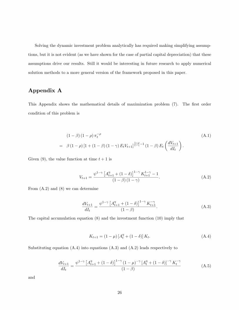
Appendix A

This Appendix shows the mathematical details of maximization problem (7). The �rst order

condition of this problem is

(1� �) (1� �)���t (A.1)

= � (1� �) [1 + (1� �) (1� )EtVt+1]1��1� �1 (1� �)Et

�dVt+1dIt

�:

Given (9), the value function at time t+ 1 is

Vt+1 = 1�

�A�t+1 + (1� �)

�1� K1� t+1 � 1

(1� �) (1� ) : (A.2)

From (A.2) and (8) we can determine

dVt+1dIt

= 1�

�A�t+1 + (1� �)

�1� K� t+1

(1� �) : (A.3)

The capital accumulation equation (8) and the investment function (10) imply that

Kt+1 = (1� �) [A�t + (1� �)]Kt: (A.4)

Substituting equation (A.4) into equations (A.3) and (A.2) leads respectively to

dVt+1dIt

= 1�

�A�t+1 + (1� �)

�1� (1� �)� [A�t + (1� �)]

� K� t

(1� �) (A.5)

and

26

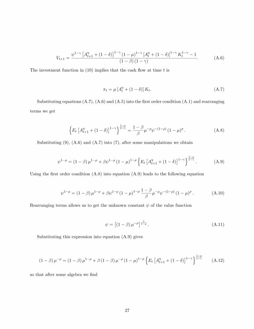
Vt+1 = 1�

�A�t+1 + (1� �)

�1� (1� �)1� [A�t + (1� �)]

1� K1� t � 1

(1� �) (1� ) : (A.6)

The investment function in (10) implies that the cash �ow at time t is

�t = � [A�t + (1� �)]Kt: (A.7)

Substituting equations (A.7), (A.6) and (A.5) into the �rst order condition (A.1) and rearranging

terms we get

nEt�A�t+1 + (1� �)

�1� o 1��1�

=1� ��

��� �(1��) (1� �)� : (A.8)

Substituting (9), (A.6) and (A.7) into (7), after some manipulations we obtain

1�� = (1� �)�1�� + � 1�� (1� �)1��nEt�A�t+1 + (1� �)

�1� o 1��1�

: (A.9)

Using the �rst order condition (A.8) into equation (A.9) leads to the following equation

1�� = (1� �)�1�� + � 1�� (1� �)1�� 1� ��

��� �(1��) (1� �)� : (A.10)

Rearranging terms allows us to get the unknown constant of the value function

=�(1� �)���

� 11�� : (A.11)

Substituting this expression into equation (A.9) gives

(1� �)��� = (1� �)�1�� + � (1� �)��� (1� �)1��nEt�A�t+1 + (1� �)

�1� o 1��1�

(A.12)

so that after some algebra we �nd

27

� = 1� �1�

�hEt�A�t+1 + (1� �)

�1� i 11� � 1��

�

(A.13)

= 1� �1�

(Et

��A�e�#t+1 + 1� �

�1� � 11� ) 1��

�

:

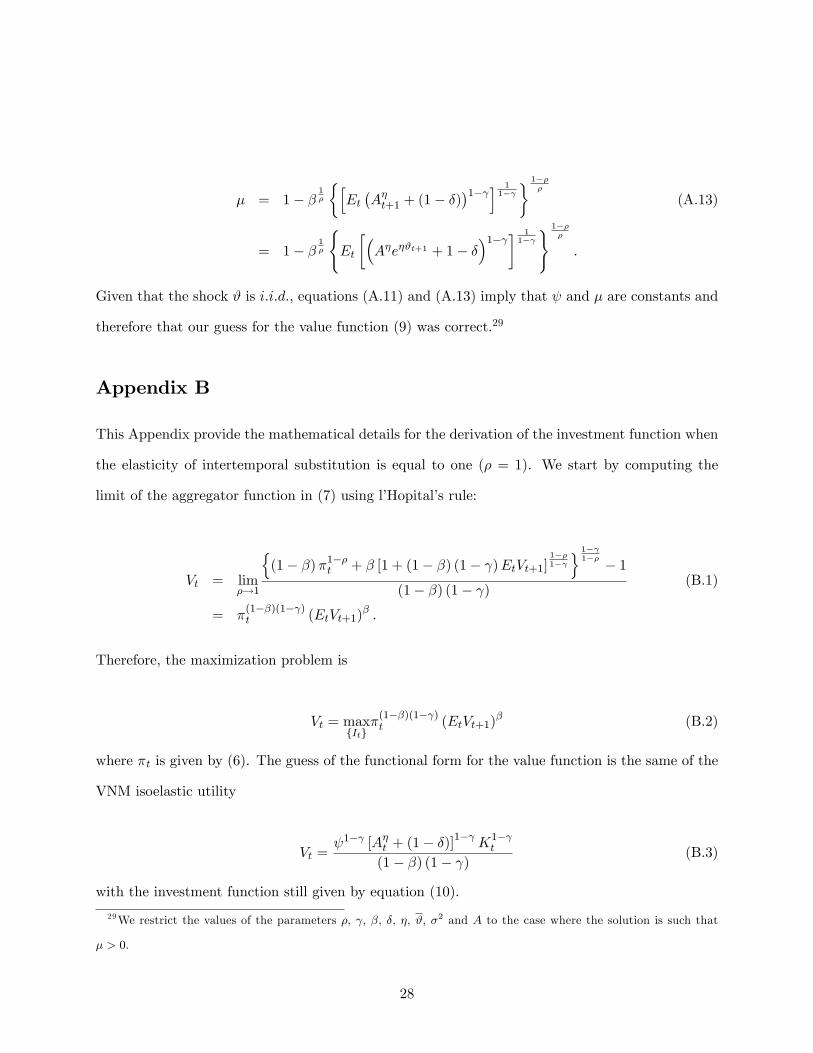
Given that the shock # is i:i:d:, equations (A.11) and (A.13) imply that and � are constants and

therefore that our guess for the value function (9) was correct.29

Appendix B

This Appendix provide the mathematical details for the derivation of the investment function when

the elasticity of intertemporal substitution is equal to one (� = 1). We start by computing the

limit of the aggregator function in (7) using l�Hopital�s rule:

Vt = lim�!1

n(1� �)�1��t + � [1 + (1� �) (1� )EtVt+1]

1��1� o 1� 1�� � 1

(1� �) (1� ) (B.1)

= �(1��)(1� )t (EtVt+1)

� :

Therefore, the maximization problem is

Vt = maxfItg

�(1��)(1� )t (EtVt+1)

� (B.2)

where �t is given by (6). The guess of the functional form for the value function is the same of the

VNM isoelastic utility

Vt = 1� [A�t + (1� �)]

1� K1� t

(1� �) (1� ) (B.3)

with the investment function still given by equation (10).

29We restrict the values of the parameters �, , �, �, �, #, �2 and A to the case where the solution is such that

� > 0.

28

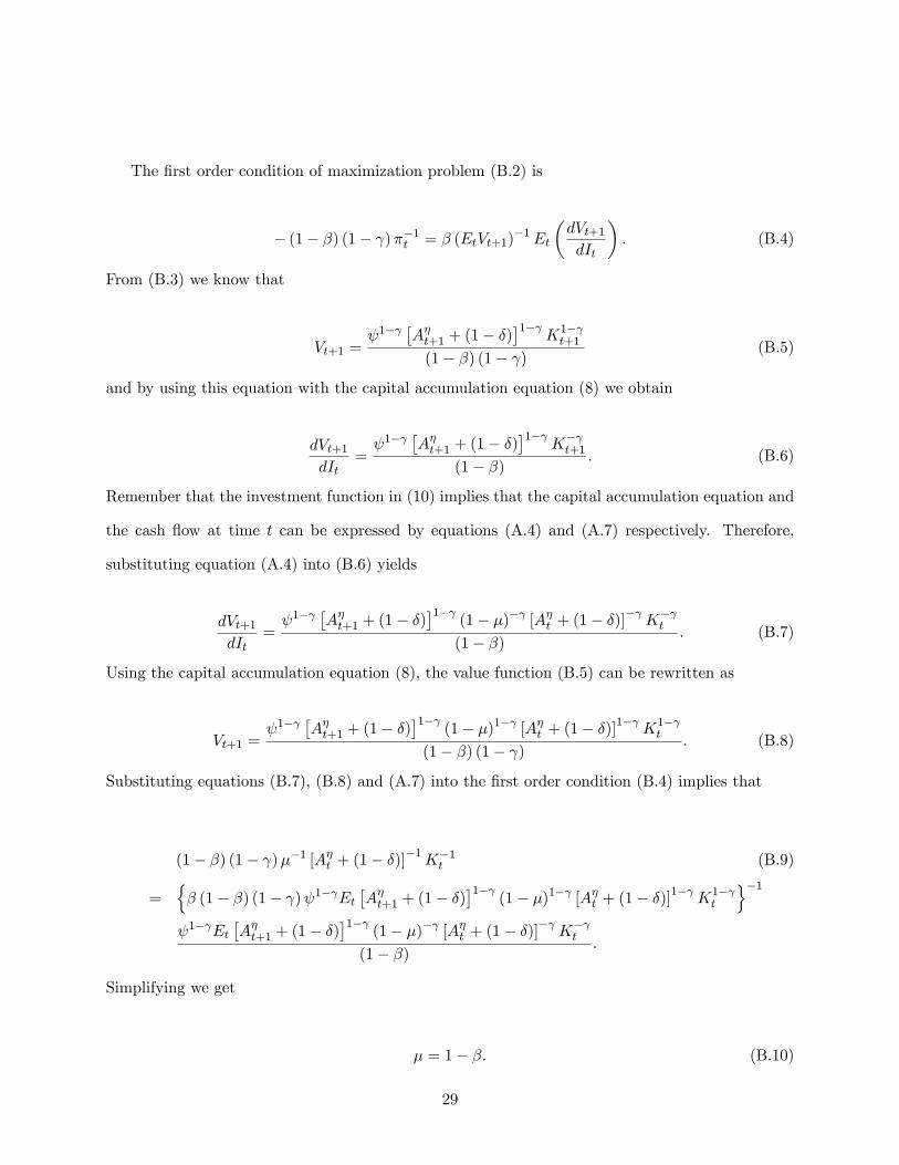
The �rst order condition of maximization problem (B.2) is

� (1� �) (1� )��1t = � (EtVt+1)�1Et

�dVt+1dIt

�: (B.4)

From (B.3) we know that

Vt+1 = 1�

�A�t+1 + (1� �)

�1� K1� t+1

(1� �) (1� ) (B.5)

and by using this equation with the capital accumulation equation (8) we obtain

dVt+1dIt

= 1�

�A�t+1 + (1� �)

�1� K� t+1

(1� �) : (B.6)

Remember that the investment function in (10) implies that the capital accumulation equation and

the cash �ow at time t can be expressed by equations (A.4) and (A.7) respectively. Therefore,

substituting equation (A.4) into (B.6) yields

dVt+1dIt

= 1�

�A�t+1 + (1� �)

�1� (1� �)� [A�t + (1� �)]

� K� t

(1� �) : (B.7)

Using the capital accumulation equation (8), the value function (B.5) can be rewritten as

Vt+1 = 1�

�A�t+1 + (1� �)

�1� (1� �)1� [A�t + (1� �)]

1� K1� t

(1� �) (1� ) : (B.8)

Substituting equations (B.7), (B.8) and (A.7) into the �rst order condition (B.4) implies that

(1� �) (1� )��1 [A�t + (1� �)]�1K�1t (B.9)

=n� (1� �) (1� ) 1� Et

�A�t+1 + (1� �)

�1� (1� �)1� [A�t + (1� �)]

1� K1� t

o�1 1� Et

�A�t+1 + (1� �)

�1� (1� �)� [A�t + (1� �)]

� K� t

(1� �) :

Simplifying we get

� = 1� �: (B.10)

29

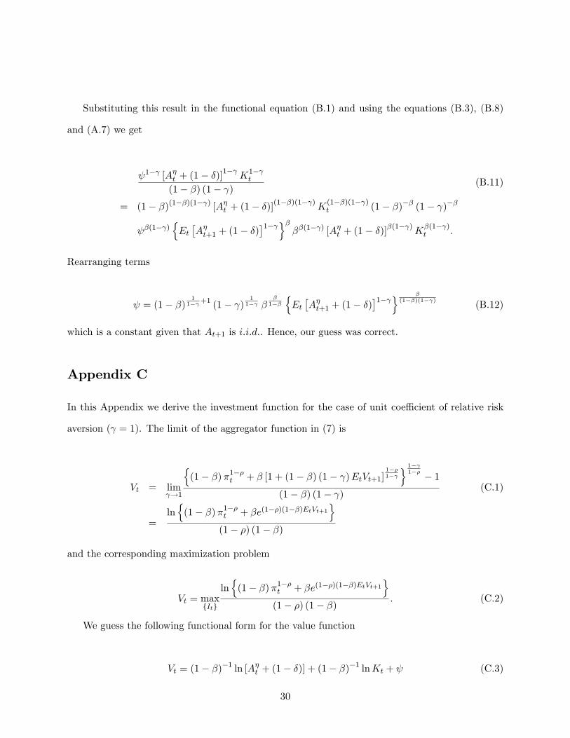
Substituting this result in the functional equation (B.1) and using the equations (B.3), (B.8)

and (A.7) we get

1� [A�t + (1� �)]1�

K1� t

(1� �) (1� ) (B.11)

= (1� �)(1��)(1� ) [A�t + (1� �)](1��)(1� )

K(1��)(1� )t (1� �)�� (1� )��

�(1� )nEt�A�t+1 + (1� �)

�1� o���(1� ) [A�t + (1� �)]

�(1� )K�(1� )t :

Rearranging terms

= (1� �)1

1� +1 (1� )1

1� ��

1��nEt�A�t+1 + (1� �)

�1� o �(1��)(1� )

(B.12)

which is a constant given that At+1 is i:i:d:. Hence, our guess was correct.

Appendix C

In this Appendix we derive the investment function for the case of unit coe¢ cient of relative risk

aversion ( = 1). The limit of the aggregator function in (7) is

Vt = lim !1

n(1� �)�1��t + � [1 + (1� �) (1� )EtVt+1]

1��1� o 1� 1�� � 1

(1� �) (1� ) (C.1)

=lnn(1� �)�1��t + �e(1��)(1��)EtVt+1

o(1� �) (1� �)

and the corresponding maximization problem

Vt = maxfItg

lnn(1� �)�1��t + �e(1��)(1��)EtVt+1

o(1� �) (1� �) : (C.2)

We guess the following functional form for the value function

Vt = (1� �)�1 ln [A�t + (1� �)] + (1� �)�1 lnKt + (C.3)

30

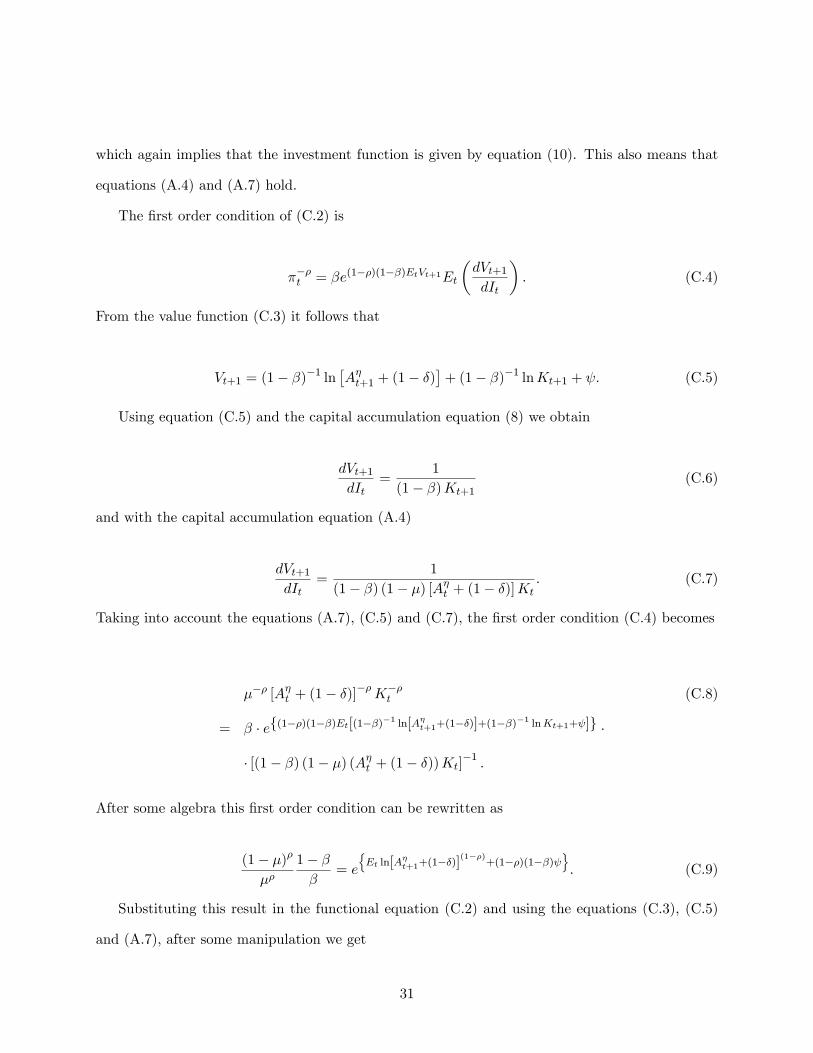
which again implies that the investment function is given by equation (10). This also means that

equations (A.4) and (A.7) hold.

The �rst order condition of (C.2) is

���t = �e(1��)(1��)EtVt+1Et

�dVt+1dIt

�: (C.4)

From the value function (C.3) it follows that

Vt+1 = (1� �)�1 ln�A�t+1 + (1� �)

�+ (1� �)�1 lnKt+1 + : (C.5)

Using equation (C.5) and the capital accumulation equation (8) we obtain

dVt+1dIt

=1

(1� �)Kt+1(C.6)

and with the capital accumulation equation (A.4)

dVt+1dIt

=1

(1� �) (1� �) [A�t + (1� �)]Kt: (C.7)

Taking into account the equations (A.7), (C.5) and (C.7), the �rst order condition (C.4) becomes

��� [A�t + (1� �)]��K��t (C.8)

= � � ef(1��)(1��)Et[(1��)�1 ln[A�t+1+(1��)]+(1��)

�1 lnKt+1+ ]g �

� [(1� �) (1� �) (A�t + (1� �))Kt]�1:

After some algebra this �rst order condition can be rewritten as

(1� �)�

��1� ��

= e

nEt ln[A�t+1+(1��)]

(1��)+(1��)(1��)

o: (C.9)

Substituting this result in the functional equation (C.2) and using the equations (C.3), (C.5)

and (A.7), after some manipulation we get

31

(1� �) [lnA�t + lnKt + (1� �) ] (C.10)

= lnn(1� �)�1��A�(1��)t K1��

t + � � e(1��) lnKt+1 � eEt lnA�t+1+(1��)(1��)

o:

Using the fact that e(1��) lnKt+1 = K1��t+1 and the �rst order condition (C.9) we obtain

(1� �) ln [A�t + (1� �)] + (1� �) lnKt + (1� �) (1� �) (C.11)

= lnf(1� �)�1�� [A�t + (1� �)]1��

K1��t +

+� (1� �)1�� [A�t + (1� �)]1��

K1��t

(1� �)�

��1� ��

g

and after some algebra

=ln (1� �)� � ln�(1� �) (1� �) : (C.12)

Substituting this expression in the maximization problem (C.2) we can recover the value of �

� = 1� �1� e

1��� fEt ln[A�t+1+(1��)]g (C.13)

which is a constant. Therefore, also is constant and this implies that our guess was correct.

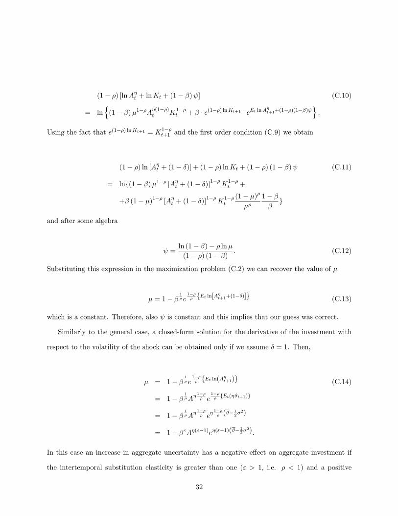
Similarly to the general case, a closed-form solution for the derivative of the investment with

respect to the volatility of the shock can be obtained only if we assume � = 1. Then,

� = 1� �1� e

1��� fEt ln(A�t+1)g (C.14)

= 1� �1�A

� 1��� e

1���fEt(�#t+1)g

= 1� �1�A

� 1��� e

� 1��� (#�

12�2)

= 1� �"A�("�1)e�("�1)(#�12�2):

In this case an increase in aggregate uncertainty has a negative e¤ect on aggregate investment if

the intertemporal substitution elasticity is greater than one (" > 1, i.e. � < 1) and a positive

32

e¤ect when " < 1. This result and the interpretation correspond to the case discussed above where

> �. Although the procedure followed has involved a transformation of the utility function, the

�nal result could be obtained directly form equations (16) and (18) substituting = 1.

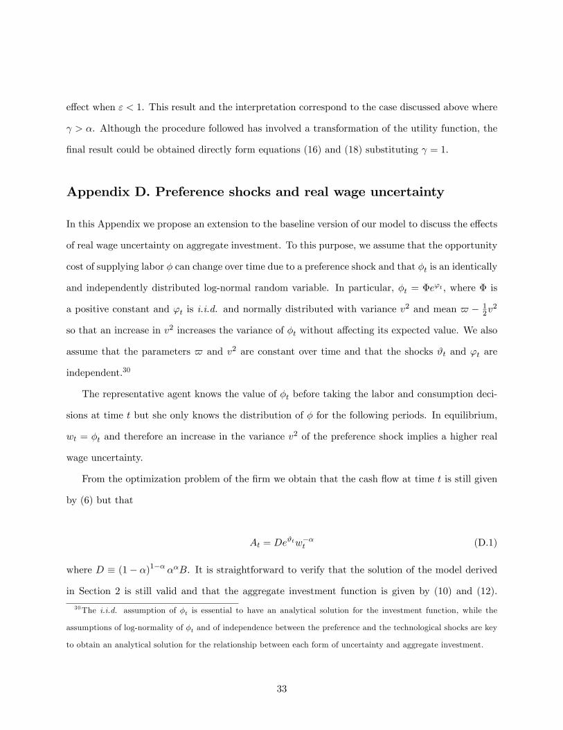
Appendix D. Preference shocks and real wage uncertainty

In this Appendix we propose an extension to the baseline version of our model to discuss the e¤ects

of real wage uncertainty on aggregate investment. To this purpose, we assume that the opportunity

cost of supplying labor � can change over time due to a preference shock and that �t is an identically

and independently distributed log-normal random variable. In particular, �t = �e't , where � is

a positive constant and 't is i.i.d. and normally distributed with variance v2 and mean $ � 1

2v2

so that an increase in v2 increases the variance of �t without a¤ecting its expected value. We also

assume that the parameters $ and v2 are constant over time and that the shocks #t and 't are

independent.30

The representative agent knows the value of �t before taking the labor and consumption deci-

sions at time t but she only knows the distribution of � for the following periods. In equilibrium,

wt = �t and therefore an increase in the variance v2 of the preference shock implies a higher real

wage uncertainty.

From the optimization problem of the �rm we obtain that the cash �ow at time t is still given

by (6) but that

At = De#tw��t (D.1)

where D � (1� �)1�� ��B. It is straightforward to verify that the solution of the model derived

in Section 2 is still valid and that the aggregate investment function is given by (10) and (12).

30The i.i.d. assumption of �t is essential to have an analytical solution for the investment function, while the

assumptions of log-normality of �t and of independence between the preference and the technological shocks are key

to obtain an analytical solution for the relationship between each form of uncertainty and aggregate investment.

33

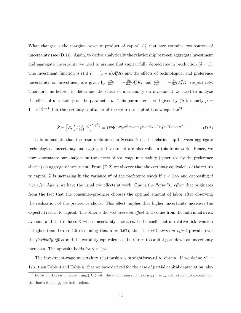
What changes is the marginal revenue product of capital A�t that now contains two sources of

uncertainty (see (D.1)). Again, to derive analytically the relationship between aggregate investment

and aggregate uncertainty we need to assume that capital fully depreciates in production (� = 1).

The investment function is still It = (1 � �)A�tKt and the e¤ects of technological and preference

uncertainty on investment are given by @It@�2

= � @�@�2

A�tKt and @It@v2

= � @�@v2

A�tKt respectively.

Therefore, as before, to determine the e¤ect of uncertainty on investment we need to analyze

the e¤ect of uncertainty on the parameter �. This parameter is still given by (16), namely � =

1� �" �Z"�1, but the certainty equivalent of the return to capital is now equal to31

�Z �hEt

�A�(1� )t+1

�i 11�

= D�����e�#���$+12(�� )�2�2+ 1

2��2(1�� )v2 : (D.2)

It is immediate that the results obtained in Section 2 on the relationship between aggregate

technological uncertainty and aggregate investment are also valid in this framework. Hence, we

now concentrate our analysis on the e¤ects of real wage uncertainty (generated by the preference

shocks) on aggregate investment. From (D.2) we observe that the certainty equivalent of the return

to capital �Z is increasing in the variance v2 of the preference shock if < 1=� and decreasing if

> 1=�. Again, we have the usual two e¤ects at work. One is the �exibility e¤ect that originates

from the fact that the consumer-producer chooses the optimal amount of labor after observing

the realization of the preference shock. This e¤ect implies that higher uncertainty increases the

expected return to capital. The other is the risk aversion e¤ect that comes from the individual�s risk

aversion and that reduces �Z when uncertainty increases. If the coe¢ cient of relative risk aversion

is higher than 1=� � 1:5 (assuming that � = 0:67), then the risk aversion e¤ect prevails over

the �exibility e¤ect and the certainty equivalent of the return to capital goes down as uncertainty

increases. The opposite holds for < 1=�.

The investment-wage uncertainty relationship is straightforward to obtain. If we de�ne � �

1=�, then Table 4 and Table 6, that we have derived for the case of partial capital depreciation, also

31Equation (D.2) is obtained using (D.1) with the equilibrium condition wt+1 = �t+1 and taking into account that

the shocks #t and 't are independent.

34

summarize the relationship between real wage uncertainty and aggregate investment under recursive

and CRRA preferences respectively. A negative relationship between real wage uncertainty and

aggregate investment under recursive preferences requires that the relative risk aversion and the

elasticity of intertemporal substitution are both relatively high or both relatively low. This is the

same result obtained with technological uncertainty. The only di¤erence is on the threshold of the

coe¢ cient of relative risk aversion � which is now (1=�) > 1 instead of � < 1. This also implies

that the region of where there is a negative correlation between investment and uncertainty under

CRRA preferences is between one and 1=�.

This analysis allows us to conclude that the existence of uncertainty on the real wage does not

change the main results of our model.

References

[1] Abel, A. B. (1983). �Optimal investment under uncertainty.�American Economic Review 73,

pp. 228-233.

[2] Abel, A. B. and J. C. Eberly (1994). �A uni�ed model of investment under uncertainty.�

American Economic Review 84, pp. 1369-1384.

[3] Abel, A. B. and J. C. Eberly (1996). �Optimal investment with costly reversibility.�Review

of Economic Studies 63, pp. 581-593.

[4] Abel, A. B. and J. C. Eberly (1997). �An exact solution for the investment and value of a �rm

facing uncertainty, adjustment costs, and irreversibility.�Journal of Economic Dynamics and

Control 21, pp. 831-852.

[5] Abel, A. B. and J. C. Eberly (1999). �The e¤ects of irreversibility and uncertainty on capital

accumulation.�Journal of Monetary Economics 44, pp. 339-377.

35

[6] Aizenman, J. and N. Marion (1993). �Policy persistence, persistence and growth.�Journal of

International Economics 1, pp. 145-163.

[7] Aizenman, J. and N. Marion (1999). �Volatility and investment: Interpreting evidence from

developing countries.�Economica 66, pp. 155-179.

[8] Alesina, A. and R. Perotti (1996). �Income distribution, political instability, and investment.�

European Economic Review 40, pp. 1203-1228.

[9] Attanasio, O. P. and G. Weber (1989). �Intertemporal substitution, risk aversion and the euler

equation for consumption.�Economic Journal 99, pp. 59-73.

[10] Barro, R. J. (1991). �Economic growth in a cross section of countries.�Quarterly Journal of

Economics 106, pp. 407-443.

[11] Bernanke, B. (1983). �Irreversibility, uncertainty and cyclical investment.�Quarterly Journal

of Economics 98, pp. 85-106.

[12] Bertola, G. (1988). �Adjustment costs and dynamic factor demands: investment and employ-

ment under uncertainty.�Ph.D. dissertation (ch. 2), Massachusetts Institute of Technology.

[13] Bloom, N., S. Bond, and J. Van Reenen (2005). �Uncertainty and investment dynamics.�

Mimeo, London School of Economics.

[14] Caballero, R. (1991). �On the sign of the investment-uncertainty relationship.�American Eco-

nomic Review 81, pp. 279-288.

[15] Calcagnini, G. and E. Saltari (2000). �Real and �nancial uncertainty and investment decisions.�

Journal of Macroeconomics 22, pp. 491-514.

[16] Craine, R. (1989). �Risky business. The allocation of capital.�Journal of Monetary Economics

23, pp. 201-218.

36

[17] Eberly, J. C. (1993). �Comment on: Economic instability and aggregate investment.�NBER

Macroeconomics Annual, pp. 303-312.

[18] Eichennbaum, M. S., L. P. Hansen, and K. J. Singleton (1988). �A time series analysis of

representative agent models of consumption and leisure choice under uncertainty.�Quarterly

Journal of Economics 103, pp. 51-78.

[19] Epstein, L. and S. Zin (1989). �Substitution, risk aversion, and the temporal behavior of

consumption and asset returns: A theoretical framework.�Econometrica 57, pp. 937-969.

[20] Epstein, L. and S. Zin (1991). �Substitution, risk aversion, and the temporal behavior of

consumption and asset returns: An empirical analysis.�Journal of Political Economy 99, pp.

263-286.

[21] Ferderer, J. P. (1993a). �The impact of uncertainty on aggregate investment.� Journal of

Money, Credit and Banking 25, pp. 30-48.

[22] Ferderer, P. J. (1993b). �Does uncertainty a¤ect investment spending?� Journal of Post Key-

nesian Economics 16, pp. 19-35.

[23] Giovannini, A. and P. Weil (1989). �Risk aversion and intertemporal substitution in the capital

asset pricing model.�National Bureau of Economic Research Working Paper No.2824.

[24] Gourinchas, P.-O. and J. A. Parker (2002). �Consumption over the life cycle.�Econometrica

70, pp. 47-89.

[25] Guiso, L. and G. Parigi (1999). �Investment and demand uncertainty.�Quarterly Journal of

Economics 114, pp. 185-227.

[26] Guo, X., J. Miao, and E. Morellec (2005). �Irreversible investment with regime shifts.�Journal

of Economic Theory 122, pp. 37-59.

[27] Hansen, L. P. and K. J. Singleton (1982). �Generalized instrumental variables estimation of

non-linear rational expectation models.�Econometrica 50, pp. 1269-1286.

37

[28] Hansen, L. P. and K. J. Singleton (1983). �Stochastic consumption, risk aversion, and the

temporal behavior of asset returns.�Journal of Political Economy 91, pp. 249-265.

[29] Hartman, R. (1972). �The e¤ects of price and cost uncertainty on investment.� Journal of

Economic Theory 5, pp. 258-266.

[30] Huizinga, J. (1993). �In�ation uncertainty, relative price uncertainty, and investment in U.S.

manufacturing.�Journal of Money, Credit, and Banking 25, pp. 521-549.

[31] Jorgenson, D.W. (1963). �Capital theory and investment behavior.�American Economic Re-

view, Papers and Proceedings 53, pp. 247�259.

[32] Kreps, D. and E. Porteus (1978). �Temporal resolution of uncertainty and dynamic choice

theory.�Econometrica 46, pp. 185-200.

[33] Kreps, D. and E. Porteus (1979). �Dynamic choice theory and dynamic programming.�Econo-

metrica 47, pp. 91-100.

[34] Leahy, J. V. and T. M. Whited (1996). �The e¤ect of uncertainty on investment: Some stylized

facts.�Journal of Money, Credit, and Banking 28, pp. 68-83.

[35] Leland, H. E. (1968). �Saving and uncertainty: the precautionary demand for saving.�Quar-

terly Journal of Economics 82, pp. 465-473.

[36] Levine, R. and D. Renelt (1992). �A sensitivity analysis of cross-country growth regressions.�

American Economic Review 82, pp. 942-963.

[37] Long, J. B. J. and C. I. Plosser (1983). �Real business cycles.�Journal of Political Economy

91, pp. 39-69.

[38] McDonald, R. and D. Siegel (1986). �The value of waiting to invest.�Quarterly Journal of

Economics 101, pp. 707-728.

38

[39] Oi, W. Y. (1961). �The desirability of price instability under perfect competition.�Economet-

rica 29, pp. 58-68.

[40] Pindyck, R. (1988). �Irreversible investment, capacity choice, and the value of the �rm.�

American Economic Review 78, pp. 969-985.

[41] Pindyck R. (1993). �A note on competitive investment under uncertainty.�American Economic

Review 83, pp. 273�277.

[42] Pindyck, R. S. and A. Solimano (1993). �Economic instability and aggregate investment.�

NBER Macroeconomics Annual, 259-303.

[43] Ramey, G. and V. A. Ramey (1995). �A cross-country evidence on the link between volatility

and growth.�American Economic Review 85, pp. 1138-1151.

[44] Sandmo, A. (1970). �The e¤ect of uncertainty on saving decisions.�Review of Economic Studies

37, pp. 353-360.

[45] Selden, L. (1978). �A new representation of preferences over certain x uncertain consumption

pairs: the ordinal certainty equivalent hypothesis.�Econometrica 46, pp. 1045-1060.

[46] Weil, P. (1989). �The equity premium puzzle and the risk-free rate puzzle.�Journal of Mone-

tary Economics 24, pp. 401-421.

[47] Weil, P. (1990). �Nonexpected utility in macroeconomics.�Quarterly Journal of Economics

105, pp. 29-42.

[48] Zeira, J. (1990). �Cost uncertainty and the rate of investment.�Journal of Economic Dynamics

and Control 14, pp. 53-63.

39

Table 1. The aggregate investment-uncertainty relationship with recursive preferences and � = 1.

dI

d�2 > � = � < �

" < 1 ; � > 1 > 0 = 0 < 0

" = 1 ; � = 1 = 0 = 0 = 0

" > 1 ; � < 1 < 0 = 0 > 0

Table 2. The aggregate investment-uncertainty relationship with CRRA preferences and � = 1.

0 < < � = � � < < 1 = 1 > 1

dI

d�2> 0 = 0 < 0 = 0 > 0

40

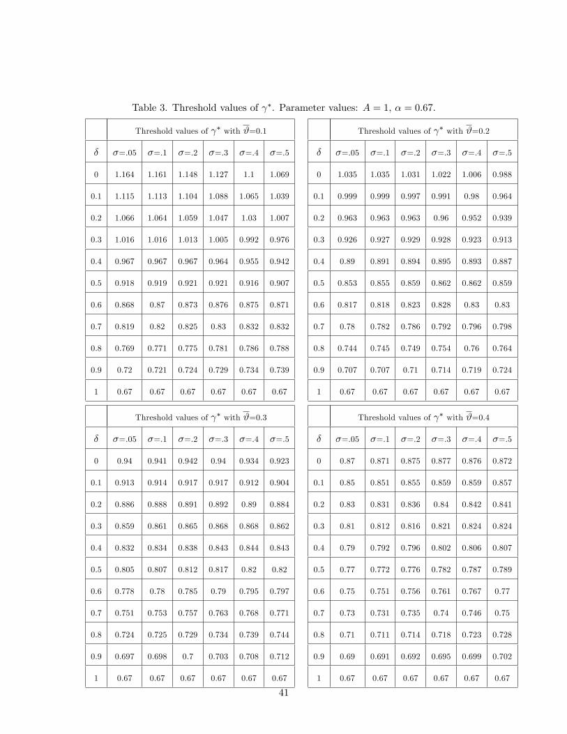
Table 3. Threshold values of �. Parameter values: A = 1, � = 0:67.

Threshold values of � with #=0.1

� �=.05 �=.1 �=.2 �=.3 �=.4 �=.5

0 1.164 1.161 1.148 1.127 1.1 1.069

0.1 1.115 1.113 1.104 1.088 1.065 1.039

0.2 1.066 1.064 1.059 1.047 1.03 1.007

0.3 1.016 1.016 1.013 1.005 0.992 0.976

0.4 0.967 0.967 0.967 0.964 0.955 0.942

0.5 0.918 0.919 0.921 0.921 0.916 0.907

0.6 0.868 0.87 0.873 0.876 0.875 0.871

0.7 0.819 0.82 0.825 0.83 0.832 0.832

0.8 0.769 0.771 0.775 0.781 0.786 0.788

0.9 0.72 0.721 0.724 0.729 0.734 0.739

1 0.67 0.67 0.67 0.67 0.67 0.67

Threshold values of � with #=0.2

� �=.05 �=.1 �=.2 �=.3 �=.4 �=.5

0 1.035 1.035 1.031 1.022 1.006 0.988

0.1 0.999 0.999 0.997 0.991 0.98 0.964

0.2 0.963 0.963 0.963 0.96 0.952 0.939

0.3 0.926 0.927 0.929 0.928 0.923 0.913

0.4 0.89 0.891 0.894 0.895 0.893 0.887

0.5 0.853 0.855 0.859 0.862 0.862 0.859

0.6 0.817 0.818 0.823 0.828 0.83 0.83

0.7 0.78 0.782 0.786 0.792 0.796 0.798

0.8 0.744 0.745 0.749 0.754 0.76 0.764

0.9 0.707 0.707 0.71 0.714 0.719 0.724

1 0.67 0.67 0.67 0.67 0.67 0.67

Threshold values of � with #=0.3

� �=.05 �=.1 �=.2 �=.3 �=.4 �=.5

0 0.94 0.941 0.942 0.94 0.934 0.923

0.1 0.913 0.914 0.917 0.917 0.912 0.904

0.2 0.886 0.888 0.891 0.892 0.89 0.884

0.3 0.859 0.861 0.865 0.868 0.868 0.862

0.4 0.832 0.834 0.838 0.843 0.844 0.843

0.5 0.805 0.807 0.812 0.817 0.82 0.82

0.6 0.778 0.78 0.785 0.79 0.795 0.797

0.7 0.751 0.753 0.757 0.763 0.768 0.771

0.8 0.724 0.725 0.729 0.734 0.739 0.744

0.9 0.697 0.698 0.7 0.703 0.708 0.712

1 0.67 0.67 0.67 0.67 0.67 0.67

Threshold values of � with #=0.4

� �=.05 �=.1 �=.2 �=.3 �=.4 �=.5

0 0.87 0.871 0.875 0.877 0.876 0.872

0.1 0.85 0.851 0.855 0.859 0.859 0.857

0.2 0.83 0.831 0.836 0.84 0.842 0.841

0.3 0.81 0.812 0.816 0.821 0.824 0.824

0.4 0.79 0.792 0.796 0.802 0.806 0.807

0.5 0.77 0.772 0.776 0.782 0.787 0.789

0.6 0.75 0.751 0.756 0.761 0.767 0.77

0.7 0.73 0.731 0.735 0.74 0.746 0.75

0.8 0.71 0.711 0.714 0.718 0.723 0.728

0.9 0.69 0.691 0.692 0.695 0.699 0.702

1 0.67 0.67 0.67 0.67 0.67 0.67

41

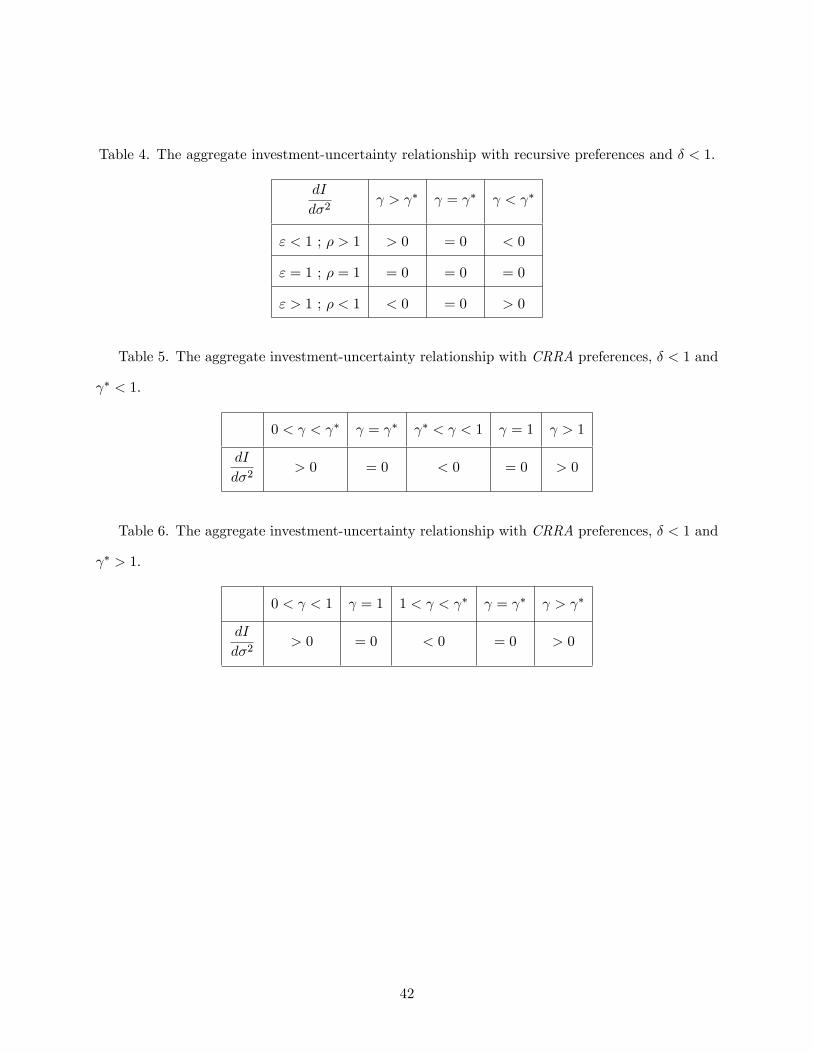
Table 4. The aggregate investment-uncertainty relationship with recursive preferences and � < 1.

dI

d�2 > � = � < �

" < 1 ; � > 1 > 0 = 0 < 0

" = 1 ; � = 1 = 0 = 0 = 0

" > 1 ; � < 1 < 0 = 0 > 0

Table 5. The aggregate investment-uncertainty relationship with CRRA preferences, � < 1 and

� < 1.

0 < < � = � � < < 1 = 1 > 1

dI

d�2> 0 = 0 < 0 = 0 > 0

Table 6. The aggregate investment-uncertainty relationship with CRRA preferences, � < 1 and

� > 1.

0 < < 1 = 1 1 < < � = � > �

dI

d�2> 0 = 0 < 0 = 0 > 0

42

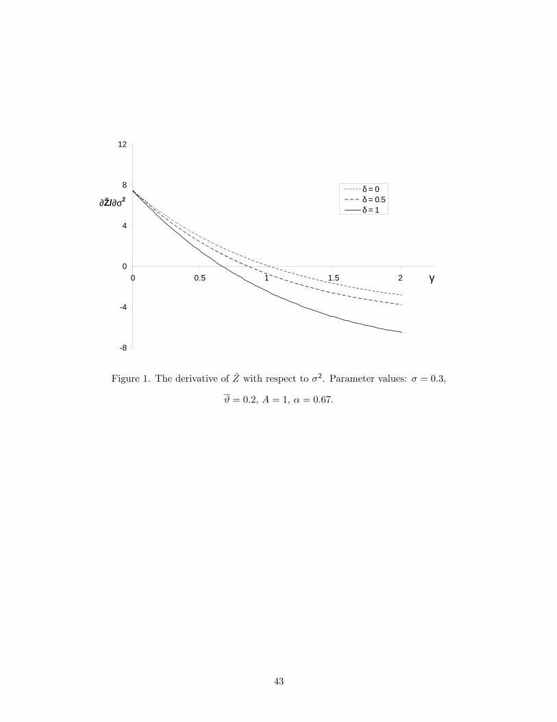
­8

­4

0

4

8

12

0 0.5 1 1.5 2

δ = 0δ = 0.5δ = 1

γ

∂Ž/∂σ2

Figure 1. The derivative of �Z with respect to �2. Parameter values: � = 0:3,

# = 0:2, A = 1, � = 0:67.

43

0.6

0.8

1

1.2

0 0.2 0.4 0.6 0.8 1

ϑ = 0.1

ϑ = 0.2

ϑ = 0.3

0.67

δ

γ∗

Figure 2. The e¤ect of a variation of # on �(�). Parameter values: � = 0:3, A = 1,

� = 0:67.

44

0.4

0.6

0.8

1

1.2

0 0.2 0.4 0.6 0.8 1

α = 0.5α = 0.67α = 0.75

δ

0.5

0.67

0.75

γ∗

Figure 3. The e¤ect of a variation of � on �(�). Parameter values: � = 0:3,

# = 0:2, A = 1.

45