For comments, suggestions or further inquiries please contact:

Philippine Institute for Development StudiesPhilippine Institute for Development Studies

The PIDS Discussion Paper Seriesconstitutes studies that are preliminary andsubject to further revisions. They are be-ing circulated in a limited number of cop-ies only for purposes of soliciting com-ments and suggestions for further refine-ments. The studies under the Series areunedited and unreviewed.

The views and opinions expressedare those of the author(s) and do not neces-sarily reflect those of the Institute.

Not for quotation without permissionfrom the author(s) and the Institute.

The Research Information Staff, The Research Information Staff, Philippine Institute for Development Studies3rd Floor, NEDA sa Makati Building, 106 Amorsolo Street, Legaspi Village, Makati City, PhilippinesTel Nos: 8924059 and 8935705; Fax No: 8939589; E-mail: publications@pidsnet.pids.gov.ph

Or visit our website at http://www.pids.gov.ph

DISCUSSION PAPER SERIES NO. 99-08

March 1999

Caesar B. Cororaton

The Philippine Tariff Structure:An Analysis of Changes,

Effects and Impacts

1

The Philippine Tariff Structure: An Analysisof Changes, Effects and Impacts1

Caesar B. Cororaton2

(First Draft, October 1998)

I. Introduction

One of the most highly controversial reforms implemented in the

Philippines in recent years is the trade reform. The trade reform program

consisted of (a) the “tariffication” of quantitative restrictions; (b) the simplification

of the tariff rate structure to a narrower rate range, and (c) the reduction in the

tariff protection. The overriding objective of the reform program is to promote

production efficiency, and therefore promote international competitiveness of the

local products. The paper discusses the effects of the program on (i) the

structure of tariff; and (ii) the effects and impacts on resource allocation, income

distribution, and on households in terms of food availability. The analysis in the

paper is based on a survey of related literature as well as on a set of model

simulations using an economy-wide model of the Philippine economy.

The reforms in the trade sector intensified beginning 1992. From

that year on to the mid-1997, the economy registered a robust economic growth

in terms of gross domestic product (see the table below). Interestingly, during the

same period, poverty incidence consistently dropped from 44.2 percent in 1985

to 35.5 percent in 1994 to 32.1 percent in 1997. There was a significant drop in

the poverty incidence in the National Capital Region (NCR) from 23.1 percent in

1985 to 8.0 percent in 1994 and further down to 7.1 percent in 1997. Although

poverty incidence in areas outside NCR also dropped over the same period the

drop was considerably lesser than NCR’s. In 1997, poverty incidence in these

areas is still very high at 36.2 percent. Furthermore, in a much poorer region, the

CAR, poverty incidence in 1997 is still above 40 percent. Clearly, there was a

deterioration in the gap between the urban and the rural areas. In fact, this is

clearly reflected in the rise of the Gini Ratio from 0.451 in 1994 to 0.496 in 1997.

Indeed, this widening gap is a major concern at present. While this could be a

1 A paper written under the Philippine-MIMAP project and presented during the MIMAP conference inKatmandu, Nepal, November 1998.2 Research Fellow, Philippine Institute for Development Studies

2

result of a host of factors that transpired during the period, certainly, it is worth

looking at whether the trade reform process contributed to this.

Philippine Economy1985 1991 1994 1997

Real GDP growth (%) -7.2 -0.6 4.4 5.2

Gini Ratio 0.446 0.468 0.451 0.496

Poverty Incidence

Philippines 44.2 35.5 32.1

NCR 23.0 8.0 7.1

Outside NCR 47.5 39.9 36.2

CAR 51.0 42.3Where NCR is National Capital region, CAR is Cordillera Autonomous Region.

II. Trade Reforms3

II.A Before 1990s.

The major turning points in trade policy reforms in the Philippines

before the 1990s took place during the following years:

(i) 1962 when the government dismantled the import and

foreign exchange restrictions.

(i) 1965 when the Philippine peso was officially devalued from

P2 to P3.9 per US dollars.

(i) However, because of persistent BOP imbalance, the foreign

exchange controls were re-imposed in 1967 and the exchange rate was

further devalued from P3.9 to P6.4 to US dollar.

3 Based on the paper of Manasan and Querubin (1997).

3

(i) In the 1973, a major tariff reform program was put in place.

The purpose of the program was to simplify the tariff rate structure to a

system of six tariff rates. However, during the same period non-tariff

measures such as quantitative restrictions (QRs) were intensified. For

example, the Central Bank prohibited the importation of consumer goods

which are classified as non-essential, unclassified or semi-classified. Also,

about the same period taxes were imposed on major traditional exports.

(v) A major trade reform program was launched in 1980. This

program has three major components: the 1981-1985 Tariff Reform

Program (TRP); the Import Liberalization Program (ILP); and the

complimentary realignment of the indirect taxes. In TRP, there was a

narrowing of the tariff rate structure from a range of 100 – 0 percent to 50

– 10 percent. During the period 1983-1985 sales taxes on imports and

locally produced goods were equalized. Also, the mark-up applied on the

value of imports (for sales tax valuation) was reduced and eventually

eliminated. Lastly, because of the balance of payments crisis during the

mid-1980s the import liberalization program was postponed. In fact, some

of the items which were deregulated earlier were re-regulated.

(vi) When the Aquino government took over in 1986, the trade

reform program of the early 1980s was resumed. In fact, the number of

regulated items was reduced from 1,802 in 1985 to 609 in 1988.

Furthermore, export taxes on all products except logs were abolished.

II.B. Within 1990s

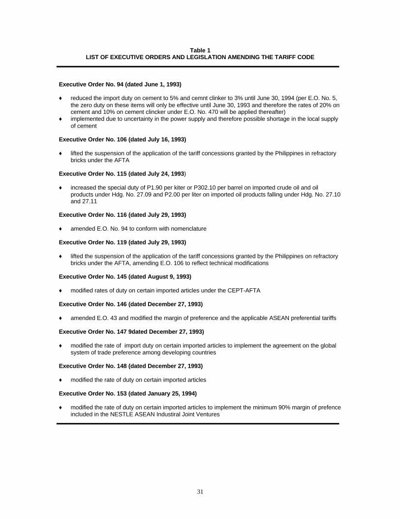
Table (1) summarizes the trade reform program during the 1990s.

The government launched a major reform program in 1991 with the issuance of

the Executive Order (EO) 470 (also called the TRP-II, an extension of the

previous trade reform program). Under this program, tariff rates were realigned

over a five-year period. The realignment involved the narrowing of the tariff rate

range through a series of reduction of the number of commodity lines with high

tariffs and an increase in the commodity lines with low tariffs. In particular, the

program was aimed at clustering the commodities with tariffs within the 10 – 30

tariff rate range by 1995. Despite the programmed narrowing of the tariff range,

4

about 10 percent of the total number of commodity lines were still subjected to 0 -

5 percent tariff and 50 percent tariff rates by the end of the program in 1995.

“Tariffication” of QRs started in 1992 with the implementation of EO

8. There were 153 commodities whose QRs were converted into tariff equivalent

rates. Also, under the same EO, tariff rates on 48 commodities were further re-

aligned. EO 8 raised the tariff rates applicable to the relevant commodities by

100 percent of their pre-EO 8 levels. In effect, the tariff rates imposed were

higher than the tariff equivalent rates in a number of cases, especially during the

initial years of the conversion. However, EO 8 has a built-in program for a five-

year phase-down of the “tariffied” rates.

Under the import liberalization program, de-regulation continued on

286 items. By the end of 1992, only 164 commodities were covered under the

QRs. However, the implementation of the Memorandum Order (MO) 95 in 1993

reversed the de-regulation process. In fact, QRs were re-imposed on 93 items,

bringing up the number of regulated items under the QR to 257. This re-

regulation came largely as the result of the Magna Carta for Small Farmers in

1991.

Major reforms were implemented under the TRP-III. The program

embodied in the following EOs: (i) EO 189 implemented in January 1, 1994 which

provided reduced tariff rates on capital equipment and machinery; (ii) EO 204 in

September 30, 1994 which mandated tariff reduction in textiles, garments, and

chemical inputs; (iii) EO 264 in July 22, 1995 which reduced tariffs on 4,142

harmonized lines (HS) in the manufacturing sector; and (iv) EO 288 in January 1,

1996 which reduced tariffs on “non-sensitive” components of the agricultural

sector. The restructuring of tariff under these EOs refers to a reduction in the

number of tariff tiers and the maximum tariff rates. In particular, the program was

aimed at establishing a four-tier tariff schedule: 3 percent for raw materials and

capital equipment which are not available locally; 10 percent for raw materials

and capital equipment that are available from local sources; 20 percent for

intermediate goods; and 30 percent for finished goods.

Another major tariff program which is in the pipeline and is likely to

be implemented starting 2004 is the uniform tariff rate. At the moment, debate is

5

still ongoing on as to the possible effects of this tariff program and at what rate

will the tariff be made uniform across sectors. Suggestion of five percent has

been put forward.

It should be emphasized at this point that analyses concerning the

impact of tariff changes generated mixed results. Some simulation results would

point to an output-augmenting tariff changes, while others would not. There are

also differentiated effects at the sectoral level. While some simulations show

favorable effects on agriculture relative to industry, and others do not. This

differentiated effects lead to differentiated effects on income distribution. In cases

where agriculture is favorable affect, households in the lower income brackets

are favorable affected as well. This is because these household groups heavily

depend on agriculture.

III. Review of Impact Studies Concerning Tariff Changes

III.A. Impact On Tariff Simplification and International

Competitiveness

In a recent paper, Manasan and Querubin (1997) analyzed the

impact of the different trade and tariff reform programs which took effect in the

1990s on tariff simplification and international competitiveness. Their analysis of

tariff simplification was based on the frequency distribution of tariff rates across

HS (harmonized system) lines, while their international competitiveness analysis

was based on mean, standard deviation, and coefficient of variation of tariff rates

and effective rates of protection (EPRs) and on the movement of the index

(1+EPR).

There is an extensive system of incentive provisions and

exemptions in the economy. Thus to account for these factors, they adjusted the

nominal tariff, as well as the implicit rates for duty exemptions (see Section V for

further discussion). Furthermore, they have two indicators for implicit tariff rates:

one, involving book rates, and, another price comparison. Price comparison

implicit tariff rates were computed using domestic prices and border prices,

where border prices were indicated by Hong Kong price and FAO prices on

selected agricultural products.

6

The study found that as a result of all these trade and tariff reform

programs, there have been significant achievements in the area of tariff

simplification. The programs transformed the tariff system from a five-level rate

schedule to a three-level rate schedule. In fact, most of the commodities cluster

around the 3-20 percent range. Moreover, the HS lines is programmed to reduce

from 6,197 in 1990 to 5,725 in 2000. This is a significant development as it

streamlines customs administration and minimizes incentives for evasion.

Based on the results of the computation, they claim that there are

some gains in terms of the reduction in the average nominal and implicit tariff

rates, as well as in the EPRs over the 1990-2000 period. Overall, the average

nominal tariff rate shall have been reduced from 33.3 percent to 19.5 percent in

2000. Likewise, the average implicit rate based on price comparison shall have

been reduced from 28.6 percent in 1990 to 16.8 percent in 2000. In addition, the

overall EPR based on price comparison shall have been reduced from 29.4

percent to 18.0 at the turn of the century.

It should be emphasized that their results indicate that the decline

in the EPRs is more pronounced for the manufacturing group than for the primary

group, particularly the agriculture sub-group. This means that there is a switch-

over in the relative protection in agriculture and manufacturing sectors. Relative

protection is found to be increasing from 1995 to 2000, in sharp contrast to the

previous decades when the agricultural sector was penalized heavily relative to

the manufacturing sector. During the period 1990-1994, the manufacturing group

enjoyed relatively higher protection than agriculture. There is a major switch

during the period 1995-2000 in favor of agriculture.

III.B. Macro and Industrial Effects

There are a number of simulations results derived using different

models analyzing some of the developments and reforms that had taken place in

the trade sector, particularly the foreign trade. This section summarizes a few of

the simulations conducted on tariff changes using different types of economic

models on the Philippines economy. Some of the tariff rate changes analyzed

were actual changes, while some are “analytical” changes. The former attempts

7

to understand the actual effects of the actual changes, while the latter tries to

understand the likely effects of some of the tariff changes programmed to be

implemented in the future. These studies are included here so as to situate, as

well as put the set of simulation results obtained in the present paper in context.

In one of the MIMAP papers Jap (1997) simulated the changes in

tariff from 1993 to 1996 using the PIDS macroeconometric model. His results

showed that total the overall output of the economy increased as a result of the

decline in the average tariff rate. In terms of the sectoral output effects, all major

sectors showed output improvement. However, there are differentiated effects

across major sectors, with Industry benefiting the most, while agriculture the least

during the simulation period.

In another paper Jap (1997) conducted another set of simulations

concerning across-the-board uniform tariff of five percent using a smaller

macroeconometric model based on a three-gap framework. In particular, the

average tariff rate is programmed to decline toward five percent by the year

2004. The results indicate a greater demand for imports which leads to

worsening of the trade deficit. This effect in turn puts pressure on the exchange

rate. However, the increase in the volume of imports does not compensate for

the reduction in the tariff level, and as such, leads to a deterioration in the fiscal

balance. In general, the implication of the analysis is that tariff reduction makes

macroeconomic constraints more restrictive, which leads to an unambiguous fall

in investment and, consequently, in a lower growth rate.

However, using a partial equilibrium, trade model based on input-

output framework, Tan (1997) found that the five percent uniform tariff has

favorable effects. Output can increase from the trade reform and from the five

percent uniform tariff as resource allocation improves within the tradable sector

due to changes in relative prices. Further simulations show that a much lower

uniform tariff (say three percent) translates to a potentially higher growth in

output and income. The growth rate for the manufacturing sector is highest, while

the decrease in output is least for agriculture. Additional insights from the

simulation results indicate that a much higher uniform tariff rate results in a

greater rate by which the output of agriculture will fall.

8

Cororaton (1995) conducted few simulations concerning changes in

the sectoral nominal and implicit tariff rates from 1988 to 1992 using the APEX

(1992) model, which is a computable general equilibrium model of the Philippine

economy. The implicit tariff rates used in the simulation exercises were computed

with the following adjustments: duty exemption, BOI incentives, duty drawback,

VAT exemptions and discriminatory excise tax.

The average annual effect on real GDP using nominal tariff rate

change is 0.47 percent increase. There is a marginal increase in inflation of 0.04

percent. However, the increase in GDP is accompanied by a 0.11 percent

increase in the current account deficit, as the increase in exports surpasses the

increase in imports. However, when the exchange rate was adjusted to bring

back the external sector in balance, the annual average growth of GDP is

reduced to 0.44 percent. This is the effect of a much higher impact on prices as

a result of the adjustment in the exchange rate.

In another paper, Cororaton (1997) conducted another round of

simulations concerning tariff changes within two different exchange rate regimes,

fixed and flexible exchange rates, using a financial computable general

equilibrium (FCGE) model of the Philippine economy constructed by Jemio and

Vos (1993). One of the major results indicate that changes in tariff within a

flexible exchange rate would have the biggest effect in terms of GDP growth.

That is, a tariff reduction program implemented within a flexible exchange rate

regime has the biggest positive effect on output. However, the effect on income

is marginal, particularly income distribution. This is probably due to the less

elaborated treatment of income in the model.

III.C. Income Distribution Effects

There are few simulation results analyzing the income distribution

effects of trade reform program in the Philippines except for two papers: Jap

(1997), and Cororaton (1995). This section summarizes the results of these

papers.

Jap (1997) extended his paper to capture the income distribution

effects of the tariff change from 1993 to 1996 by extending his macroeconometric

9

model with an income distribution sub-model. The income sub-model is driven by

the sectoral gross value added results of the main macro model. The income

distribution effects as indicated by the Gini Ratio shows a deterioration in income

distribution. One possible reason for this type of effect can be observed if one

links this results with his sectoral output. As discussed above, the industrial

sector registered the biggest positive increase in output. Although the output of

the agricultural sector increased as well, its rate of increase was far below the

industrial sector. Since households in the lower income brackets in the

Philippines heavily depend on the agricultural sector, the relatively slower growth

in agriculture naturally generates unfavorable income distribution effects.

Cororaton (1995) generated some income distribution simulation

results concerning tariff changes from 1988 and 1992 using the same APEX

model cited above. The results would indicate some progressivity in the tariff

change during the period, i.e., households in the lowest income group enjoyed

the highest increase in income compared to the highest income group. The

progressivity in the tariff change was more pronounced in the results on

households labor income. These results hold for both fixed and flexible exchange

rates.

Furthermore, the progressiveness of the tariff change could be

explained by the results on prices of unskilled labor, skilled labor, and the price of

variable capital. For both fixed and flexible exchange rate regimes, unskilled

labor gets the highest increase in wages. Unskilled labor usually belongs to the

poorest segment of the population. Furthermore, the price of capital increases a

lot faster than the general price of labor. Since substitution between labor and

capital is allowed in the model, the higher increase in the price of capital relative

to the price of labor resulted in some kind of a substitution effect in favor of labor.

This effect partly explained the favorable income distribution effects.

III.D. Household Effects

There is only one paper available which looked at the household

effects of the tariff change. Using a linking matrix, which links the results of a

CGE model on sectoral prices and household incomes with household model on

nutrition outcome (discussed in more detail in the next section), Orbeta and Alba

10

(1996) quantified the calorie and protein availability effects in different household

types as a result of the tariff changes between 1988 and 1992. In particular, they

utilized the results of the APEX model simulations on sectoral prices and

household incomes concerning the said tariff change between these two years.

They arrived at a set of results which indicate that except for beverages, prices

decline as a result of the tariff program between 1988 and 1992. The income

change shows that the same tariff program has progressive effects as lower

income households received higher income increase compared to the higher

income households.

Through the use of the linking matrix which they developed, they

were able to compute for the change in the demand for food resulting from the

price and income changes. As a result of the decline in prices, household

increase their demand for most of the food items except for the highest income

quintile where only the demand for cereal, fish and other food increase.

Furthermore, they translated these effects into changes in calorie and protein

availability in households. The set of results they arrived would indicate that the

1988-1992 tariff reform program was not only progressive in terms of income, but

also equally progressive in terms of macro nutrient availability in households. In

particular, lower income households are shown to have greater increase in both

calorie and protein availability.

IV. Brief Description of the Model

IV.A. Economy-Wide Model of the Philippines

The results of the simulation presented in this paper were derived

using the 34-sector economy-wide developed by Cororaton (1997). Appendix 1

discusses the basic structure of the model. It is important to emphasize here that

the model is still in a development stage at the moment. Although the model can

be used to analyze policy changes as such tariff changes, it does not capture at

the moment some of the institutional rigidities in the actual economy. For

example, both factor and product markets are price-clearing, making the model

very neoclassical in spirit. In the labor market, for example, there is no

unemployment. Both wages and labor adjust to clear the market for any shock

introduced into the system. Therefore, the issue of unemployment as a result of

11

changes in policies, such as tariff reforms, although very important concern in

MIMAP, is not yet captured in the model. However, efforts are currently

undertaken to modify the specification of them model to be able to capture these

nuances. Furthermore, the model is a one-period model. As such it cannot

capture the “dynamic” effects of a policy shock. Because of these, the results of

the simulations are preliminary in nature. Further simulation runs will be

conducted after some of these modifications are incorporated into the model.

Results will then be compared with the results obtained here.

IV.B. Linking Matrix

Orbeta (1994) developed a framework4 for simulating the effects of

food policies in which three types of policy instruments were identified: supply

shifters, demand shifters, and price wedges. From an estimated demand curves

for food (qi), the percentage change in quantities demand can be expressed as:

• • •(1) qi = Σn

jeijpdj + γiy i = 1, ..., n

where the dots (•) indicate percentage changes, eij direct and cross-price

elasticities of demand; pdj demand price; γi income elasticity of demand; and y

income. On the other hand, supply changes can be represented as

• •(2) qi = Σn

jsijpsj + δi i = 1, ..., n

where sij are the supply elasticities, psj supply price and δi supply shift variable.

Moreover, to allow for price subsidies, the equilibrium relationship

can be written as

• • •(3) ps

i = pdi + βi i = 1, ..., n

4The framework was originally developed by Quisumbing (1985).

12

where βi is the size of subsidy wedge for commodity i.

In matrix form these three sets of n equations can be expressed as

(4) • •-H O I Pd Γy • O -S I Ps = ∆ • •-I I O Q B

where

H : n x n matrix of demand elasticities, eij

S : n x n matrix of supply elasticities, sij

Pd: n x 1 vector of demand prices, pdi

Ps: n x 1 vector of supply prices, psi

Q : n x 1 vector of quantities, qi

Γ : n x 1 vector of income elasticities of demand, γi

∆ : n x 1 vector of supply shifts, δi

B : n x 1 vector of price subsidies, βi

The solution for the changes in equilibrium prices and quantities as

a function of the policy variables can be expressed as

(5) • • •

Pd (S-H)-1(Γy - ∆ - SB)• • •Ps = (S-H)-1(Γy - ∆ - HB)• • •Q H(S-H)-1(SH-1Γy - ∆ - SB)

Thus, given the changes in the equilibrium consumption of

commodities, the percentage change in the equilibrium level of nutrient

consumption is

• • • •(6) N = K Q = K { H(S-H)-1(SH-1Γy - ∆ - SB) }

13

where K is an 1 x n vector of Ki, the fraction of initial total nutrient consumption

provided by commodity i. This equation serves as the linking equation, while Q

as the linking matrix.

This framework would allow one to compute for the changes in

calorie and protein consumption under policy changes affecting the market for

food. The parameters of the matrix are derived from the household models

estimated by Orbeta and Alba (1996).

V. Empirical Results

The objective of the paper is to analyze the income distribution and

resource allocation effects of implicit tariff changes from 1990 to 2000. To date a

number of tariff programs have been put in place. As discussed above, a number

of Executive and Memorandum Orders have been put into effect since 1991.

While Manasan and Querubin (1997) analyzed the impact of these programs

both on implicit tariff rate and effective rate of protection in their paper, they did

not look into the effects on income distribution and resource allocation. Tariff

changes lead to changes in relative output and factor prices. Because of these

changes resources would move across sectors and would in turn lead to

changes in resource allocation. Furthermore, changes in relative factor prices

affect income of institutions and therefore income distribution. The paper will

attempt to understand the effects of these changes using a 34-sector economy-

wide model of the Philippine economy

The simulations were conducted using 1988 implicit tariff rates in

the base run. The effects of the tariff change from 1990 to 2000 were compared

with the base run using percentage difference. It should be emphasized that the

model is not dynamic, but a one-year, static model. Thus, the annual results were

derived from independent simulation runs of the model using the annual implicit

tariff rates from 1990 to 2000 discussed below.

V.A. Computation of Implicit Tariff Rates

The analysis starts with the implicit tariff rates computed by

Manasan and Querubin (1997). The sectoral Implicit tariff rates were computed

14

using price comparison wherein domestic prices are compared with border

prices. In particular, the formula used to compute for the implicit tariff rate for

commodity/product j is given by

(7) Tj = Pd / Pb -1

where Pd is domestic wholesale price obtained from the National Statistics Office

and the Bureau of Agricultural Statistics, and Pb is data on border prices from

Hongkong Trade Statistics and FAO.

The implicit tariff rate derived using the above formula were

adjusted for duty exemption. The formula for adjustment is given by

(8) Tjadj = (Tj Mj – Dj) / Mj

where Tjadj is the duty exempted implicit tariff rate of commodity/product j; Tj is

the computed implicit tariff rate; Mj total imports of sector j for a given year; Dj is

the value of revenue foregone from duty exemptions of imports of sector j.

Data used to compute for the price comparison estimates were

available for the years 1990-1995 only. To smoothen out year-to-year

fluctuations, the average price relatives in the three-year period ending in the

current year was used in estimating implicit tariff rates. For example, the average

price ratios for 1991, 1992 and 1993 were used to estimate the implicit tariff rate

for 1993. Moreover, the relative price estimates obtained for 1995 were assumed

to hold in 1995-2000 for the remaining regulated items in estimating the “price

comparison” implicit tariff rates.

Manasan and Querubin estimated the implicit tariff rates with

adjustments for 169 sectors. To make sectors consistent with the sectors of the

model, further aggregation was made here to 34 sectors. The aggregation used

import-plus-output as weights. This system of weighting overcomes the biases

associated with output weights or import weights alone. To facilitate the analysis,

the rates were further aggregated into 5 major sectors: total agriculture; mining;

total manufacturing, food manufacturing and other manufacturing.

15

The implicit tariff rates for the 5 major sectors are shown in Figure

1. One can observe that there is a general decline in the implicit tariff rates in all

major sectors starting 1995. Food manufacturing still has the highest implicit tariff

rate level, while mining has the lowest. In 1992, the implicit tariff rate of

agriculture crossed the declining rate of other manufactures. It increased up to

1994 and started to decline in 1995. From 1996 to 2000, its implicit tariff rate is

above other manufactures but below total manufactures

V.B. Simulation Results

Table 2 shows the effects of changes in implicit tariff on income

distribution. The results presented in the table are percent difference in the share

of household income between the scenarios (implicit tariff rates from 1990 to

2000) and the base. To facilitate the analysis, focus on the period totals. From

1990 to 1994, changes in the implicit tariff rates were generally progressive, i.e.,

households under group 1 (first decile) up to household group 7 (seventh decile)

enjoyed a positive total increase in their share of the income pie. The last three

household groups, 8 to 10, suffered a decline in the share. Note that the last

three groups are the richest income groups.

However, during the period 1995 and 1996, the change in the

implicit tariff rates were highly regressive. The poor income groups suffered a

decline in the share in the income pie, while the rich enjoyed an increase.

Looking back at Figure 1, one can observe that it was during these years when

the implicit tariff rates on agriculture registered the biggest drop.

From 1996 to 2000, the effects reversed to favor the poor

household groups. The first group up to the seventh registered an increase in

their respective income share, while the eighth to the tenth household group

suffered a decline. The share of the second group increased the most among the

household groups which enjoyed an increase in the share. However, the lowest

increase is seen in the seventh, followed by the first household group.

On the whole, the change in the implicit tariff rates can be generally

considered progressive, except for the first decile, the poorest among the poor.

For the entire period, 1990 to 2000, the last three income groups suffered a

16

decline in their income share, while the second to the seventh income groups

enjoyed an increase. Unfortunately, unfavorable effects are observed in the first

decile. Its income share declined by -1.7 percent over the entire period.

Table 3 shows the absolute change in the income of households

from the base. The progressivity of the tariff change is more pronounced in the

period 1990-1994 with the first five income groups enjoying above two percent

increase in income from the base. The increase in income for the last two groups

from the base is less than 1 percent. An opposite picture is seen in 1995 and

1996. The tariff change during the period is highly regressive. The poor income

groups (first to fourth) suffered a decline in their respective absolute income from

the base, while the rich ones (eighth to tenth) enjoyed a positive increase.

Favorable effects are observed in the period 1996-2000.

Over the entire period, 1990-2000, all income groups enjoyed an

increase in their absolute income from the base as a result of the tariff change.

However, the lowest increase in seen in the poorest household, the first group.

Thus, while its share to the total income pie declined relative to the other income

groups, the fact that its absolute income increased relative to the base would

indicate that the tariff reform programs, especially in the second half of the

1990s, is generally favorable.

Table 4 presents the percent change in consumption of the different

household groups relative to the base. Almost the same pattern is observed as in

the previous table, except that the rich groups show higher increase in

consumption than the poor groups over the entire period.

The results on factor prices presented in Table 5 will help explain

the pattern of income distribution effects seen above. Presented in the table are

results on agricultural wages (WAAG); non-agricultural wages (WANAG); price of

mixed factor (RENTMX); and price of capital (RENTKAP). Again focus on the

period totals. In the period 1994, one of the things that triggered the progressive

effects is the relatively high increase in WAAG. During the period it increased by

9.7 percent, which is a lot higher than the other three factor prices. One should

note that lower income groups heavily depend on agricultural labor, thus an

increase in agricultural wage will naturally benefit them.

17

In the succeeding two years, 1995 and 1996, the effect on WAAG

is negative. In fact it declined by a big -14.7 percent. Furthermore, the price of

mixed factor declined by –5.3 percent. The major suppliers of these two factors

of production are households in the lower groups. Thus, the decline in income

both in terms of absolute and of distribution share of these groups during the

period can largely be attributed to the decline in the prices of these factors.

In the next period ,1996-2000, all factor prices increased. However,

the price of capital showed the highest increase of 18.3 percent. The reason why

the lower income groups were favorably affected during the period is the 12.9

percent increase in the price of mixed factor. Over the entire period, 1990-2000,

the increase WANAG and RENTKAP, were far greater than the increase in

WAAG and RENTMX.

Table 6 shows the resource allocation effects of the tariff change.

The numbers in the table are percent difference in the sectoral share of output

and factor inputs between the results of the annual implicit tariff runs and the

base run. There is a general pattern of resource movement that can be observed

from the results. It involves a general resource movement from agriculture and

construction to manufacturing and utilities. This is reflected in the negative

numbers for agriculture and construction and positive for the rest of the sectors,

particularly manufacturing, for almost all periods considered. In particular, for the

entire period, 1990-2000, the share of agriculture to the total output declined by –

31 percent, while construction dropped by –22.7 percent. The share of total

manufacturing increased by 10.6 percent over the same period. Specifically, the

share of other manufacture increased by 15.2 percent, while the share of utilities

increased by a big 38.8 percent.

Factor inputs moved generally in the same manner, i.e., labor,

mixed factor, and capital moved from agriculture and construction to

manufacturing and utilities. Among the three factor inputs, it was mixed factor of

agriculture which registered the biggest drop.

Table 7 presents the absolute change in sectoral output and factor

inputs from the base value. Similar pattern holds as in the previous table, i.e., a

18

resource movement from agriculture and construction to manufacturing and

utilities. The resource movement, particularly from agriculture, is one of the major

factors behind the declining income share of the first household to the total

income pie. This group heavily depends on both agriculture labor and mixed

income. The effect was more pronounced in 1995 and 1996 when both income

share and absolute income of the poor household groups (first to the fifth)

dropped.

V.C. Household Effects: Calorie and Protein Availability

The results of economy-wide model simulations concerning tariff

changes were translated into changes in food availability in households through

the use of the linking matrix discussed in the previous section. In particular,

results on output prices and income of households were translated into protein

and calorie availability in households. However, few preliminary steps were done

to translate the changes into nutrition effects:

(1) The nutrition model estimated by Orbeta and Alba (1997) (upon

which the parameters of the linking matrix were based), has the following food

and non-food items in the specification: cereals; fruits; meat; dairy and eggs;

beverage; other food, and non-food items. To link these with the sectors in the

economy-wide model the following sector conversion was made (note: the

sectors in the economy-wide were aggregated to sectors in the household model

using value of sectoral output in the base run)

Sectors in Nutrition Model Sectors in Economy-Wide Model

Cereals Palay and Corn

Rice and Corn Milling

Fruits Fruits

Meat Meat Manufacturing

Dairy and Eggs Livestock and Poultry

Fish Fishery

Fish Manufacturing

Beverage Beverage and Tobacco

Other Foods Coconut and Sugar

Sugar Milling

Other Food

Non-Food Rest of the Sectors in the Model

19

(2) Household groups in the nutrition model were classified in

quintile. However, in the economy-wide model households were grouped in

decile. To link the model groups the following conversion was made

Households in Nutrition Model Households in Economy-wide Model

First Quintile First and Second Decile

Second Quintile Third and Fourth Decile

Third Quintile Fifth and Sixth Decile

Fourth Quintile Seventh and Eighth Decile

Fifth Quintile Ninth and Tenth Decile

The nutrition effects of the tariff change are shown in Table 8. The

results are absolute changes from the base (not percent difference). Again focus

on the period totals. One can observe that for the period 1990-1994, the results

are all positive for all five households in terms of protein and calorie availability.

However, looking closely at the magnitude of the change per household, the

impact is regressive, i.e., the fifth quintile benefited the most in terms of both

protein and calorie availability. This set of results is opposite to what was found in

Table 2, the effect on income distribution where it was observed that for the

period 1990-1994, lower income groups enjoyed increases in their income share.

These two sets of results would indicate that the positive effect on income for the

lower income group was not enough to offset the change in food prices as a

result of the tariff change. Indeed, in Table 9 prices of food manufactures

increased by 14.5 percent from the base, higher than other sectors except

services. It would also be interesting to note at this point that although all implicit

tariff rates registered a general decline during the period, the implicit tariff rate on

food manufacturing is still the highest among all major groups.

The effect on the lower income groups during the period 1995-1996

was worst: not only it was regressive in terms of income distribution, it was also

regressive in terms of protein and calorie availability. Lower income groups

witnessed an absolute decline in income as well as in food availability.

In the period 1996-2000, all household registered negative change

in calorie availability. However, the decline in the first household was lower than

20

in the second to the fifth household. However, over the same period, the effect

on protein availability is clearly regressive, as the lower income groups suffered a

decline, while the higher income groups enjoyed an increase.

Over the entire period, the impact on both protein and calorie

availability, based on the methodology adopted in the paper, was highly

regressive. Some of the lower income groups suffered a decline both in terms of

protein and calorie availability. However, over the same period, the effect on

income distribution was progressive, as observed above, except for the poorest

of the poor, the first household group. This implies that the generally favorable

income effects could not offset the unfavorable price effects on food.

VI. Summary of Results

One of the major policy reforms (often times highly controversial)

implemented in the Philippines in recent periods concerns reforms in the trade

sectors. The reforms consisted of “tariffication” of quantitative restrictions,

simplification of tariff structure from a wide rate range to a limited rate range, and

reduction in the overall tariff rate. The idea behind the reform process is (i) to

promote production efficiency; (ii) to achieve better and efficient allocation of

resources through market mechanisms; (iii) and to increase the competitiveness

of the local products. A number of papers have analyzed the impact of changes

in the trade reforms. In fact, part of the present paper is a review of the

simulation results available in the literature which attempted to explain the impact

and effect of trade reforms.

Based on the review it was observed that while the series of trade

reform programs pursued by the government led to a general decline both in the

tariff rate and the effective rate of protection as well as to a much simpler tariff

rate structure with a narrower rate range, the impact on output, income

distribution, resource allocation and households are mixed. Some results have

found that the trade reforms are progressive, while others regressive. Some have

indicated that the trade reform programs are output-augmenting, while others are

not.

21

The simulation results presented in the paper using the 34-sector

economy-wide model concerning the change in implicit tariff over the period

1990-2000 showed that the impact on income distribution is generally

progressive, except on the first decile, the lowest income group. The income

share of the second to the seventh income groups increased, while the share of

the eighth to the tenth declined during the entire period. The income share of the

first decile declined.

However, there are differences within sub-periods. During the sub-

period 1990-1994, the tariff change was progressive. Households within the

lower income brackets enjoyed higher income shares, while those within the

higher incomes suffered a decline. During 1995 and 1996, years when implicit

tariff on agriculture dropped significantly, the impact on income distribution was

highly regressive. Lower income groups witnessed not only a sharp drop in their

income share but also in their absolute income level relative to the base level.

This effect, however, was reversed during 1996-2000 to favor the lower income

groups.

The differentiated effects on income distribution across households

and within different sub-periods can be explained by changes in factor prices and

movement of resources across sectors. Based on the results, periods within

which the impact of the tariff change is progressive, it was observed that the

effect on agricultural wage and rent on mixed income is favorable. This is evident

during 1990-1994 and 1996-2000. Conversely, during periods when the impact

on these factor prices are unfavorable, the effect on the poor is also observed to

be unfavorable. This impact is pronounced during 1995 and 1996. Incidentally, it

was also during these years when the agricultural sector witnessed the biggest

drop in implicit tariff rate relative to other sectors.

During the entire simulation period, 1990-2000, there was a

resource movement from agriculture and construction to industry (particularly

manufacturing) and service sectors. Output of the former dropped, while output

of the latter increased. The drop in the former could, in turn, be explained by the

drop in mixed factor input, and to a limited extent, to the slight drop in labor.

Since households in the lower income groups (particularly, the first decile)

heavily depend on income from these factors, this type of resource movement,

22

together with the impact on factor prices, translates into unfavorable income

distribution effects. Again, this is quite evident during 1995 and 1996.

Furthermore, one of the major reasons behind the unfavorable effect on the first

decile in terms of income distribution is the movement of resources away from

agriculture to industry.

An attempt was made to translate this set of effects on households,

particularly on food availability in households in terms of protein and calorie

availability through use of a linking matrix whose parameters were derived from

the nutrition model estimated by Orbeta and Alba. On the whole the results

indicate a great deal of regressivity in food availability. Over the entire period, the

first to the third quintile suffered an absolute decline in protein availability, while

the fourth and fifth enjoyed an improvement. In terms of calorie availability, only

the first quintile suffered a absolute decline. This is the effect despite the

increase in the absolute income of all households from the base run. The

dampening effect on food availability in household came from the increase in

food prices as well as from the increase in food-related agricultural commodities.

It may probably be worth mentioning at this point that while almost all sectors

have declining implicit tariff rates, the food sector still has the highest rates even

up to the turn of the century.

Caveat. The paper does not attempt to calculate the impact of the

trade reform program. It only attempts to understand the mechanisms, the

channels, and the direction of change through which the trade reform affects

resource allocation, income distribution, and food availability in households. It

was observed that while the results available in the literature are quite mixed, the

results of obtained here are generally progressive in terms of income distribution

(except for the first decile) and highly regressive in terms of food availability in

households. These results were obtained from a model which is quite

disaggregated in terms of sectoral breakdown, but still limited in terms of model

specification. The important MIMAP issue of unemployment, for example, is not

yet incorporated in the model, although efforts are underway to incorporate this.

Thus, at this point the results are still preliminary. Further simulations will be

conducted after the modifications on the model specification are incorporated.

23

Appendix 1

Economy-Wide Model of thePhilippine Economy

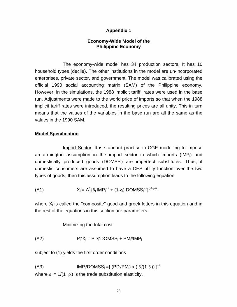
The economy-wide model has 34 production sectors. It has 10

household types (decile). The other institutions in the model are un-incorporated

enterprises, private sector, and government. The model was calibrated using the

official 1990 social accounting matrix (SAM) of the Philippine economy.

However, in the simulations, the 1988 implicit tariff rates were used in the base

run. Adjustments were made to the world price of imports so that when the 1988

implicit tariff rates were introduced, the resulting prices are all unity. This in turn

means that the values of the variables in the base run are all the same as the

values in the 1990 SAM.

Model Specification

Import Sector. It is standard practise in CGE modelling to impose

an armington assumption in the import sector in which imports (IMPi) and

domestically produced goods (DOMSSi) are imperfect substitutes. Thus, if

domestic consumers are assumed to have a CES utility function over the two

types of goods, then this assumption leads to the following equation

(A1) Xi = Aci{δI IMPi

-ρi + (1-δi) DOMSSi-ρi}(-1/ρi)

where Xi is called the "composite" good and greek letters in this equation and in

the rest of the equations in this section are parameters.

Minimizing the total cost

(A2) Pi*Xi = PDi*DOMSSi + PMi*IMPi

subject to (1) yields the first order conditions

(A3) IMPi/DOMSSi ={ (PDi/PMi) x ( δi/(1-δi)) }σi

where σi = 1/(1+ρi) is the trade substitution elasticity.

24

From (A3) the consumers will choose a combination of IMPi and

DOMSSi depending upon their relative prices; domestic price, PMi, and domestic

price of imports, PMi.

The domestic price of imports is linked with the world price of

imports (PWMi) through the following relationship

(A4) PMi = PWMi*(1+TMi)*ER

where ER is the exchange rate and TMi is the import tariff rate.In the system of

equations, Equations (A1) to (A3) are all expressed explicitly.

Export Sector. The model assumes that Philippine exports (EXPi)

face a constant elasticity demand function.

(A5) EXPi = E0*(Ai/PEi)ηi

where E0 is constant, Ai is world price of i, and PEi is the domestic price of

exports. There is a divergence between the export price and the domestic price

of the goods through the following equation

(A6) PEi = PWEi*ER/(1+TEi)

where PWEi is the world price of export, and TEi is export tax.

Domestic Production. Domestic production of good i is described by

a Cobb-Douglas production function with 3 types of factor inputs: labor (LBi),

mixed factor, (MXi), and capital, KAPi.

(A7) DOMSSi =Ai*LBiαi*MXi

βi*KAPi(1-αi-βi)

Demand for Factor Inputs. Assuming perfect competition, profit

maximization requires that each of the factor price should equal to the value of

the marginal product. Thus, for the labor factor we have

(A8) WA*LBi = XDi*PVAi

25

where WA is the average wage rate and PVAi is the net value added price which

is defined as

(A9) PVAi = PXi - EjIOij*PXj - (ITAXi + DEPXDi + IMPXDi)

where IOij in the input-output technical coefficient matrix, ITAXi indirect tax rate,

DEPXDi ratio between depreciation and output, and IMPXDi ratio between

imports and total output.

For the mixed factor we have

(A10) RENTMX*MXi = XDi*PVAi

where RENTMX is the average mixed factor rent. Lastly, for capital we have

(A11) RENTKAP*LBi = XDi*PVAi

where RENTKAP is the average capital rent

The supply of each of these factors are assumed fixed. Therefore,

each of the factors is cleared through changes in each of the respective factor

prices. If the demand for a given factor decreases, given fixed supply, the factor

price would have to adjust to clear the market. Changes in factor prices are

relevant to issues on income distribution. Furthermore, the market for agricultural

labor is separated from the market for non-agricultural labor. This means that

there are two separate average market clearing wages; one for the agricultural

sector and another for non-agricultural.5 Again, this is relevant to the income

distribution analysis.

Further refinements of the model may have to be done. For

example, the labor market may have to be modified to account for some wage

rigidity mechanisms. Instead of a market clearing wage, a partial adjustment 5Note that in the future extension of the model, these two labor markets may be linked and augmentedto account for labor migration from the agricultural sector to industry and service sectors. This is alsorelevant to the analysis on adjustment policies and income distribution.

26

mechanism may be imposed so that wages may not clear the labor market

instantaneously. Thus, quantity adjustments through unemployment changes

need to be invoked to somehow clear the market within a period. This

specification will therefore allow for unemployment analysis, which is relevant to

the issue on income distribution. Furthermore, if a Phillips curve equation is

attached to unemployment, the delayed response in wage adjustment can be

linked to changes in macroeconomic policies such as monetary policy. This is

one channel whereby the link between the real and the financial sectors of the

model can be strengthened. In CGE literature, this is equivalent to imposing non-

homogeneity condition in the system.

Income of Institutions. The incomes of the institutions, except

government, have the same specification. The equation is simply the sum of all

sources of incomes: (1) factor incomes, which is the product of the market

clearing factor prices and the factor endowments of each of the institutions

(which are fixed within a given period); (2) secondary incomes, which is the

product of a fixed coefficient matrix derived from the SAM and the incomes of the

institutions, net of direct taxes (note that in the original SAM some of these

incomes are dividends and equities incomes); (3) remittances of workers

working abroad; (4) foreign transfers; and (5) other fixed incomes which are

derived using fixed coefficient from the SAM.

Income of the government is derived from the following sources: (1)

tariff revenue; (2) export tax revenue (if positive) or export subsidy (if negative);

(3) indirect tax; (4) income from its capital endowment; (5) secondary income,

derived similarly as in the other institutions; (6) foreign transfers; and (7) other

fixed incomes which are derived using fixed coefficient similar to the other

institutions.

Consumption of Institutions. The consumption (CCinst) is uniformly

specified for all institutions, except government. It is given by

(A12) CCinst,i = CLESinst*APCDOMinst*Yinst(1-DTAXinst)/PXi

27

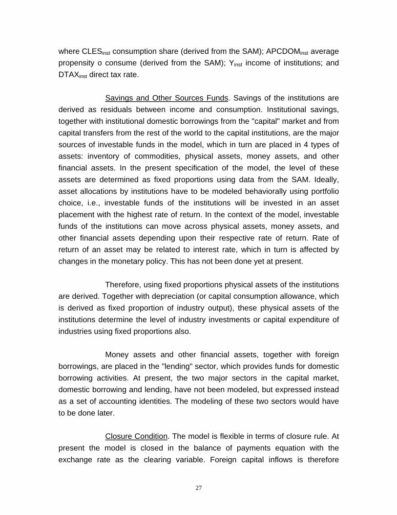
where CLESinst consumption share (derived from the SAM); APCDOMinst average

propensity o consume (derived from the SAM); Yinst income of institutions; and

DTAXinst direct tax rate.

Savings and Other Sources Funds. Savings of the institutions are

derived as residuals between income and consumption. Institutional savings,

together with institutional domestic borrowings from the "capital" market and from

capital transfers from the rest of the world to the capital institutions, are the major

sources of investable funds in the model, which in turn are placed in 4 types of

assets: inventory of commodities, physical assets, money assets, and other

financial assets. In the present specification of the model, the level of these

assets are determined as fixed proportions using data from the SAM. Ideally,

asset allocations by institutions have to be modeled behaviorally using portfolio

choice, i.e., investable funds of the institutions will be invested in an asset

placement with the highest rate of return. In the context of the model, investable

funds of the institutions can move across physical assets, money assets, and

other financial assets depending upon their respective rate of return. Rate of

return of an asset may be related to interest rate, which in turn is affected by

changes in the monetary policy. This has not been done yet at present.

Therefore, using fixed proportions physical assets of the institutions

are derived. Together with depreciation (or capital consumption allowance, which

is derived as fixed proportion of industry output), these physical assets of the

institutions determine the level of industry investments or capital expenditure of

industries using fixed proportions also.

Money assets and other financial assets, together with foreign

borrowings, are placed in the "lending" sector, which provides funds for domestic

borrowing activities. At present, the two major sectors in the capital market,

domestic borrowing and lending, have not been modeled, but expressed instead

as a set of accounting identities. The modeling of these two sectors would have

to be done later.

Closure Condition. The model is flexible in terms of closure rule. At

present the model is closed in the balance of payments equation with the

exchange rate as the clearing variable. Foreign capital inflows is therefore

28

exogenous. Net foreign capital inflows (i.e., net of current account financing) go

into the investable fund equation.

29

References

Cororaton. 1997 Tariff and Direct Household Taxes: An Economy-Wide Model

Analysis. MIMAP Research Paper Series

Cororaton. 1996 Simulating the Income Distribution Effects of the 1988-1992

Tariff Reduction Using the APEX Model. PIDS Discussion Paper

Series

Jemio and Vos. 1993 External Shocks, Debt and Adjustment: A Computable

General Equilibrium Model for the Philippines. Working Paper –

Sub-Series on Money, Finance and Development – No 45 Institute

of Social Studies.

Manasan and Querubin, 1997. Assessment of the Tariff Reform in the Nineties.

PIDS Discussion Paper Series

Orbeta 1994 Towards a Model for Analyzing the Impact of Macroeconomic

Adjustment Policies on Households: A Review of Empirical

Household Models in the Philippines. MIMAP Research Paper

Series.

Orbeta and Alba 1996. Simulating the Impact of Macroeconomic Policy Changes

on the Nutrition Status of Households. MIMAP Research Paper

Series

Quisumbing 1995. Estimating the Distributional Impact of Food Market

Intervention on Policies on Nutrition. Ph.D. Dissertation UP School

of Economics

Tan 1997. Effects of the Five Percent Uniform Tariff. PIDS Discussion Paper

Series 97-17.

Yap 1996. An Income Distribution Bloc for Macroeconomic Analysis. MIMAP

Research Paper Series

Yap. 1997 Structural Adjustment, Stabilization Policies and Income Distribution in

the Philippines: 1986-1996. MIMAP Research Paper Series

30

Table 1LIST OF EXECUTIVE ORDERS AND LEGISLATION AMENDING THE TARIFF CODE

Executive Order No. 470 (dated July 1991)

♦ increases number of commodity line with high tariffs♦ reduces number of commodity line with low tariffs

Executive Order No. 478 (dated August 23, 1991)

♦ imposes special duties of P0.95 per liter of P151.05 per barrel on imported crude oil falling under Hdg.No. 27.09 and P1.00 per liter on imported oil products.

Executive Order No. 1 (dated June 30, 1992)

♦ reduces rates of import duty on electric generating sets to 0% until June 30, 1995.♦ intended to provide partial remedy to the energy crisis.

Executive Order No. 2 (dated July 1, 1992)

♦ extends the affectivity of the zero rate of duty on cement and cement clinker up to June 30, 1995 (undere.o. No. 470, these articles will be subjected to rates of duty of 20% and 10%, respectively, beginningJuly 1, 1992)

♦ intended to stop possible shortage of localy supply if zero duty will be lifted

Executive Order No. 5 (dated July 14, 1992)

♦ shortens the operation of the zero rate of import duty on cement and cement clinker from June 30, 1995(as provided in E.O. No. 2) to June 30, 1993.

Executive Order No. 8 (dated July 24, 1992)

♦ provided for interim increased tariff protection in lieu of import restrictions♦ items covered include livestock, meat, fish, crustaceans, mollusks, sausages and other prepared meat,

cane or beet sugar, maize, cereal grains, air or vacuum pumps, fans, aircon, refrigerators/freezers,centrifuges, washing machines, sewing machines, electric accumulators, thermionic/cold cathode,public transport type passenger motor vehicle and parts.

♦ import restrictions lifted on November 1, 1992.

Memorandum Order No. 60 (dated November 5, 1992)

♦ held in abeyance until February 28, 1993 the implementation of E.O. No. 8 with respect to maize

Executive Order No. 43 (dated December 29, 1992)

♦ modified the rate of import duty on certain imported articles to implement the 1991 and 1992 Philprogram submitted to the Third ASEAN summit providing a minimum level of 25% margin of preference.

Executive Order No. 61 (dated February 27, 1993)

♦ modified the nomenclature and tariff rates on certain agricultural products; animals fresh chilled orfrozen, corn and feedwheat

♦ in line with R.A. No. 7607 (The Magna Carta of Small Farmers)

31

Table 1LIST OF EXECUTIVE ORDERS AND LEGISLATION AMENDING THE TARIFF CODE

Executive Order No. 94 (dated June 1, 1993)

♦ reduced the import duty on cement to 5% and cemnt clinker to 3% until June 30, 1994 (per E.O. No. 5,the zero duty on these items will only be effective until June 30, 1993 and therefore the rates of 20% oncement and 10% on cement clincker under E.O. No. 470 will be applied thereafter)

♦ implemented due to uncertainty in the power supply and therefore possible shortage in the local supplyof cement

Executive Order No. 106 (dated July 16, 1993)

♦ lifted the suspension of the application of the tariff concessions granted by the Philippines in refractorybricks under the AFTA

Executive Order No. 115 (dated July 24, 1993)

♦ increased the special duty of P1.90 per kiter or P302.10 per barrel on imported crude oil and oilproducts under Hdg. No. 27.09 and P2.00 per liter on imported oil products falling under Hdg. No. 27.10and 27.11

Executive Order No. 116 (dated July 29, 1993)

♦ amended E.O. No. 94 to conform with nomenclature

Executive Order No. 119 (dated July 29, 1993)

♦ lifted the suspension of the application of the tariff concessions granted by the Philippines on refractorybricks under the AFTA, amending E.O. 106 to reflect technical modifications

Executive Order No. 145 (dated August 9, 1993)

♦ modified rates of duty on certain imported articles under the CEPT-AFTA

Executive Order No. 146 (dated December 27, 1993)

♦ amended E.O. 43 and modified the margin of preference and the applicable ASEAN preferential tariffs

Executive Order No. 147 9dated December 27, 1993)

♦ modified the rate of import duty on certain imported articles to implement the agreement on the globalsystem of trade preference among developing countries

Executive Order No. 148 (dated December 27, 1993)

♦ modified the rate of duty on certain imported articles

Executive Order No. 153 (dated January 25, 1994)

♦ modified the rate of duty on certain imported articles to implement the minimum 90% margin of prefenceincluded in the NESTLE ASEAN Industiral Joint Ventures

32

Table 1LIST OF EXECUTIVE ORDERS AND LEGISLATION AMENDING THE TARIFF CODE

Executive Order No. 160 (dated February 23, 1994)

♦ reduced the special duties on crude oil products from p1.90 to P0.95 under Hdg. No. 27.09 and fromp2.00 to P1.00 on imported oil products falling under Hdg. No. 27.10 and 27.11

Executive Order No. 172 (dated April 24, 1994)

♦ increased the minimum tariff rate from 0% to 3%

Executive Order No. 189 (dated July 18, 1994)

♦ modifies the nomenclature and rates of duty on capital equipment from 10%-20% to 3%-10% (Note:major changes)

Executive Order No. 204 (dated September 30, 1994)

♦ modifies the nomenclature and rates of duty on textile and chemical input thereto (Note: major changes)

Executive Order No. 227 (dated March 4, 1995)

♦ reduced the import duty on Portland cement (3%), cement clinker 93%), and Pozzolan Cement (10%);this suspends the implementation of the 20% and 10% under E.O. 470

Executive Order No. 264 (dated July 22, 1995)

♦ modified the nomenclature and rates of duty on manufacturing industries in line with the Tariff ReformProgram; involves 4142 HS lines (Note: major changes)

Executive Order No. 287 (dated January 1, 1996)

♦ modified the rate of duty on cetain imported articles to implement the 1996 Philippine schedule of tariffreductions under the new frame of the accelerated CEPT scheme for the AFTA

Executive Order No. 288 (dated December 12, 1995)

♦ modified the nomenclature and rates of import duty on certain imported articles, i.e., non-sensitiveagricultural products; (Note: major changes)

Executive Order No. 313 (dated March 29, 1996)

♦ modified the nomenclature and rates of import duty on certain imported articles, i.e., sensitiveagricultural products;

♦ implements tariffication after import restrictions were lifted under R.A. 8178♦ IRR only issued on July 1 and effective July 10, 1996♦ Note: major changes

Executive Order No. 328 (dated (April 23, 1996)

♦ modified the nomenclature and rates import duty on imported wheat for food

Executive Order No. 365 (dated (April 16, 1996)

♦ modified the rates of duty on crude oil (from 10% to 3%) and refined petroleum product from 20% to7%).

33

Summary results of Economy-Wide Model runs involving implicit tariff changes from 1988 to 2000(base run: 1988)

Period TotalsTable 2. Income distribution effects (percent difference in household income share between scenario and base) 1990 - 1990 - 1995 - 1996 - 1990 -

1990 1991 1992 1993 1994 1995 1996 1997 1998 1999 2000 1995 1994 1996 2000 2000HH1 -0.22% 0.37% -0.61% 0.46% 0.73% -2.86% -1.74% 1.18% -0.80% 0.60% 1.14% -2.1% 0.7% -4.6% 0.4% -1.7%HH2 -0.17% 0.40% -0.42% 0.55% 0.88% -2.53% -1.03% 1.40% -0.75% 0.81% 1.60% -1.3% 1.2% -3.6% 2.0% 0.7%HH3 -0.15% 0.34% -0.34% 0.48% 0.77% -2.12% -0.82% 1.20% -0.62% 0.71% 1.42% -1.0% 1.1% -2.9% 1.9% 0.9%HH4 -0.12% 0.30% -0.28% 0.43% 0.67% -1.85% -0.70% 1.12% -0.48% 0.66% 1.31% -0.8% 1.0% -2.5% 1.9% 1.1%HH5 -0.07% 0.21% -0.17% 0.29% 0.46% -1.17% -0.38% 0.85% -0.28% 0.51% 0.98% -0.4% 0.7% -1.5% 1.7% 1.2%HH6 -0.03% 0.12% -0.07% 0.18% 0.25% -0.73% -0.27% 0.49% -0.07% 0.27% 0.60% -0.3% 0.5% -1.0% 1.0% 0.7%HH7 0.02% -0.03% 0.09% 0.01% -0.04% 0.16% 0.09% -0.11% 0.16% -0.06% -0.01% 0.2% 0.1% 0.3% 0.1% 0.3%HH8 0.09% -0.11% 0.16% -0.10% -0.24% 0.68% 0.12% -0.58% 0.49% -0.39% -0.55% 0.5% -0.2% 0.8% -0.9% -0.4%HH9 0.06% -0.17% 0.18% -0.19% -0.34% 0.97% 0.39% -0.70% 0.29% -0.40% -0.70% 0.5% -0.5% 1.4% -1.1% -0.6%HH10 0.02% -0.08% 0.04% -0.17% -0.21% 0.58% 0.28% -0.23% -0.01% -0.11% -0.38% 0.2% -0.4% 0.9% -0.4% -0.3%

34

Summary results of Economy-Wide Model runs involving implicit tariff changes from 1988 to 2000(base run: 1988)

Period TotalsTable 3. Changes in household income level (scenario vs base) 1990 - 1990 - 1995 - 1996 - 1990 -

1990 1991 1992 1993 1994 1995 1996 1997 1998 1999 2000 1995 1994 1996 2000 2000HH1 -0.16% 0.57% -0.69% 0.94% 1.44% -2.98% -0.12% 1.54% 0.22% 2.10% 5.92% -0.9% 2.1% -3.1% 9.6% 8.8%HH2 -0.12% 0.59% -0.51% 1.03% 1.60% -2.64% 0.60% 1.76% 0.27% 2.31% 6.40% 0.0% 2.6% -2.0% 11.3% 11.3%HH3 -0.09% 0.53% -0.43% 0.97% 1.49% -2.24% 0.81% 1.56% 0.40% 2.21% 6.21% 0.2% 2.5% -1.4% 11.2% 11.4%HH4 -0.06% 0.50% -0.36% 0.91% 1.39% -1.96% 0.93% 1.48% 0.54% 2.15% 6.10% 0.4% 2.4% -1.0% 11.2% 11.6%HH5 -0.01% 0.41% -0.25% 0.77% 1.18% -1.29% 1.26% 1.21% 0.74% 2.01% 5.76% 0.8% 2.1% 0.0% 11.0% 11.8%HH6 0.03% 0.31% -0.15% 0.66% 0.97% -0.85% 1.37% 0.85% 0.95% 1.75% 5.35% 1.0% 1.8% 0.5% 10.3% 11.2%HH7 0.08% 0.16% 0.00% 0.49% 0.67% 0.03% 1.74% 0.24% 1.19% 1.42% 4.71% 1.4% 1.4% 1.8% 9.3% 10.8%HH8 0.15% 0.09% 0.07% 0.38% 0.47% 0.55% 1.76% -0.23% 1.52% 1.09% 4.15% 1.7% 1.2% 2.3% 8.3% 10.0%HH9 0.12% 0.02% 0.10% 0.29% 0.37% 0.85% 2.04% -0.35% 1.32% 1.08% 4.00% 1.7% 0.9% 2.9% 8.1% 9.8%HH10 0.07% 0.11% -0.04% 0.31% 0.50% 0.46% 1.93% 0.13% 1.02% 1.37% 4.33% 1.4% 0.9% 2.4% 8.8% 10.2%

35

Summary results of Economy-Wide Model runs involving implicit tariff changes from 1988 to 2000(base run: 1988)

Table 4. Changes in consumption (scenario vs base) 1990 - 1990 - 1995 - 1996 - 1990 -1990 1991 1992 1993 1994 1995 1996 1997 1998 1999 2000 1995 1994 1996 2000 2000

HH1 -0.16% 0.57% -0.69% 0.94% 1.44% -2.98% -0.12% 1.54% 0.22% 2.10% 5.92% -0.88% 2.10% -3.10% 9.65% 8.77%HH2 -0.14% 0.68% -0.38% 0.97% 1.56% -2.45% 0.96% 1.76% 0.12% 2.33% 6.50% 0.24% 2.69% -1.49% 11.67% 11.91%HH3 -0.09% 0.66% -0.19% 0.92% 1.55% -1.85% 1.63% 1.71% 0.18% 2.33% 6.53% 1.01% 2.86% -0.22% 12.38% 13.40%HH4 -0.08% 0.65% -0.06% 0.84% 1.39% -1.51% 1.83% 1.69% 0.25% 2.30% 6.46% 1.23% 2.75% 0.32% 12.52% 13.76%HH5 -0.03% 0.58% 0.07% 0.70% 1.21% -0.76% 2.31% 1.44% 0.43% 2.17% 6.18% 1.78% 2.54% 1.55% 12.53% 14.31%HH6 0.04% 0.49% 0.25% 0.64% 1.06% -0.21% 2.66% 1.28% 0.63% 2.02% 5.95% 2.26% 2.47% 2.45% 12.54% 14.80%HH7 0.11% 0.32% 0.44% 0.50% 0.80% 0.74% 3.18% 0.82% 0.86% 1.77% 5.44% 2.90% 2.17% 3.92% 12.06% 14.97%HH8 0.21% 0.22% 0.55% 0.46% 0.69% 1.35% 3.41% 0.57% 1.23% 1.56% 5.07% 3.47% 2.13% 4.76% 11.84% 15.31%HH9 0.23% 0.09% 0.60% 0.46% 0.70% 1.70% 3.89% 0.74% 1.07% 1.71% 5.15% 3.78% 2.08% 5.59% 12.56% 16.34%HH10 0.33% 0.03% 0.27% 0.58% 1.19% 1.27% 4.27% 1.58% 0.89% 2.33% 5.96% 3.68% 2.41% 5.55% 15.03% 18.71%

36

Summary results of Economy-Wide Model runs involving implicit tariff changes from 1988 to 2000(base run: 1988)

Period TotalsTable 5. Changes in prices of factors (scenario vs base) 1990 - 1990 - 1995 - 1996 - 1990 -

1990 1991 1992 1993 1994 1995 1996 1997 1998 1999 2000 1995 1994 1996 2000 2000WAAG -0.70% 1.30% -0.60% 4.60% 5.10% -11.00% -3.70% -0.30% 0.10% 1.40% 9.50% -1.30% 9.70% -14.70% 7.00% 5.70%WANAG 0.30% -0.70% 1.70% 0.20% -0.50% 5.50% 5.60% -2.60% 3.00% 0.40% 3.50% 6.50% 1.00% 11.10% 9.90% 16.40%RENTMX -0.40% 0.70% -1.10% 0.50% 1.20% -5.00% -0.30% 4.40% -1.90% 3.30% 7.40% -4.10% 0.90% -5.30% 12.90% 8.80%RENTKAP 0.60% 0.80% 0.40% 1.00% 2.40% 5.70% 5.70% -0.30% 4.10% 2.90% 5.90% 10.90% 5.20% 11.40% 18.30% 29.20%

37

Summary results of Economy-Wide Model runs involving implicit tariff changes from 1988 to 2000(base run: 1988)

Table 6. Resource allocation effects I. Resource allocation effects (percent difference in sectoral output share between scenario and base) 1990 - 1990 - 1995 - 1996 -

1990 1991 1992 1993 1994 1995 1996 1997 1998 1999 2000 1995 1994 1996 2000Agriculture -1.07% -0.10% -0.29% -2.21% -3.40% -12.10% -6.24% -6.24% 1.19% -1.24% 0.67% -19.17% -7.07% -18.34% -11.85%Mining 0.13% 0.15% 1.99% 0.78% 1.97% 1.57% -0.09% -0.09% 0.58% 0.77% 0.02% 6.59% 5.02% 1.48% 1.19%Total Mfg 0.36% 0.15% -0.61% 0.96% 1.54% -0.08% 2.88% 2.88% -2.28% -1.21% 6.05% 2.32% 2.40% 2.79% 8.32% Mfg - food 0.71% -0.01% -1.98% 0.38% -2.34% -0.09% 3.18% 3.18% -5.12% -3.46% 9.65% -3.33% -3.24% 3.09% 7.44% Mfg - others 0.12% 0.26% 0.34% 1.37% 4.25% -0.08% 2.66% 2.66% -0.29% 0.36% 3.54% 6.27% 6.35% 2.59% 8.94%Construction -0.10% -0.04% 0.49% -0.64% -0.39% 3.96% -2.09% -2.09% 0.76% -1.31% -21.24% 3.29% -0.67% 1.87% -25.98%Utilities 0.75% 0.06% 9.60% 5.45% -6.48% 10.57% -3.75% -3.75% 8.47% 9.31% 8.61% 19.95% 9.38% 6.82% 18.90%Services 0.01% -0.02% -1.12% -0.30% 0.60% -0.88% 1.21% 1.21% -0.84% -0.23% 4.30% -1.71% -0.83% 0.33% 5.67%

II. Resource allocation effects (percent difference in sectoral labor factor demand share between scenario and base) 1990 - 1990 - 1995 - 1996 -1990 1991 1992 1993 1994 1995 1996 1997 1998 1999 2000 1995 1994 1996 2000

Agriculture -0.11% -0.66% 0.91% 0.19% 0.49% -2.27% 1.39% 1.39% -6.38% -4.02% 5.76% -1.47% 0.80% -0.88% -1.86%Mining 0.15% 0.10% 3.07% 1.03% 3.31% 4.18% 2.90% 2.90% -7.34% -3.07% -3.59% 11.83% 7.65% 7.08% -8.19%Total Mfg 0.71% 0.56% -1.54% 2.80% 4.44% 0.55% 6.50% 6.50% -7.59% -0.80% 15.56% 7.52% 6.97% 7.05% 20.18% Mfg - food 0.78% 1.59% -0.73% 3.84% 2.37% 4.84% 6.71% 6.71% -9.61% -1.83% 20.43% 12.69% 7.85% 11.55% 22.42% Mfg - others 0.64% -0.59% -2.45% 1.64% 6.75% -4.23% 6.27% 6.27% -5.34% 0.34% 10.15% 1.76% 5.99% 2.04% 17.69%Construction -0.05% -0.07% 0.08% -0.73% -0.58% 3.82% -1.14% -1.14% 0.23% -0.97% -17.25% 2.47% -1.35% 2.68% -20.26%Utilities 0.90% 0.05% 9.31% 5.42% -6.50% 11.72% -2.19% -2.19% 7.39% 9.66% 13.98% 20.91% 9.19% 9.53% 26.65%Services -0.15% 0.09% -1.75% -0.52% 0.28% -5.19% -0.06% -0.06% 1.82% 0.85% 11.44% -7.24% -2.05% -5.25% 14.00%

III. Resource allocation effects (percent difference in sectoral capital factor demand share between scenario and base) 1990 - 1990 - 1995 - 1996 -1990 1991 1992 1993 1994 1995 1996 1997 1998 1999 2000 1995 1994 1996 2000

Agriculture -1.14% 0.77% 1.45% 3.30% 4.21% -12.26% -9.22% -9.22% 3.27% 5.88% 5.18% -3.67% 8.58% -21.47% -4.11%Mining 0.20% -0.31% 3.87% 0.69% 2.54% 5.96% 3.23% 3.23% -7.23% -3.90% -8.07% 12.95% 6.99% 9.20% -12.73%Total Mfg 0.43% 1.29% 0.60% 2.87% 2.13% 5.75% 6.92% 6.92% -6.77% -2.23% 11.73% 13.06% 7.31% 12.66% 16.57% Mfg - food 0.34% 1.64% 0.26% 3.40% 1.91% 6.09% 7.66% 7.66% -9.06% -3.87% 13.81% 13.64% 7.55% 13.75% 16.21% Mfg - others 0.76% -0.11% 1.94% 0.74% 3.05% 4.37% 3.94% 3.94% 2.37% 4.34% 3.43% 10.74% 6.37% 8.32% 18.04%Construction 0.00% -0.48% 0.86% -1.06% -1.32% 5.60% -0.82% -0.82% 0.35% -1.81% -21.09% 3.60% -2.00% 4.78% -24.20%Utilities 0.96% -0.36% 10.17% 5.07% -7.19% 13.64% -1.88% -1.88% 7.52% 8.73% 8.68% 22.28% 8.64% 11.76% 21.18%Services -0.06% -0.10% -1.84% -1.02% -0.08% -3.76% -0.26% -0.26% 1.05% 0.23% 5.54% -6.86% -3.10% -4.02% 6.29%

IV. Resource allocation effects (percent difference in sectoral mixed factor demand share between scenario and base) 1990 - 1990 - 1995 - 1996 -1990 1991 1992 1993 1994 1995 1996 1997 1998 1999 2000 1995 1994 1996 2000

Agriculture -1.22% 0.08% -0.20% -1.04% -1.88% -14.26% -9.35% -9.35% 3.85% -2.44% -1.32% -18.51% -4.25% -23.61% -18.62%Mining 0.60% -0.32% 5.93% 1.49% 2.73% 13.11% 5.42% 5.42% -9.35% -3.48% -12.17% 23.54% 10.43% 18.53% -14.17%Total Mfg 1.33% -1.26% 0.24% 1.60% 3.03% 8.09% 6.00% 6.00% -5.87% -2.22% 6.56% 13.04% 4.95% 14.09% 10.47% Mfg - food 0.60% -0.82% 0.07% 4.33% 4.80% 10.70% 4.21% 4.21% -6.21% -4.16% 7.81% 19.68% 8.99% 14.91% 5.85% Mfg - others 2.73% -2.10% 0.56% -3.53% -0.30% 3.18% 9.37% 9.37% -5.23% 1.44% 4.21% 0.53% -2.65% 12.55% 19.16%Construction 0.41% -0.50% 2.86% -0.27% -1.13% 12.72% 1.28% 1.28% -1.95% -1.39% -24.61% 14.09% 1.37% 14.00% -25.39%Utilities 0.00% 0.00% 0.00% 0.00%Services 0.23% 0.04% -0.14% 0.21% 0.40% 2.55% 2.00% 2.00% -0.60% 0.75% 1.35% 3.30% 0.75% 4.55% 5.51%

38

Summary results of Economy-Wide Model runs involving implicit tariff changes from 1988 to 2000(base run: 1988)

Table 7: Period totalsChanges in sectoral output (scenario vs base) 1990 - 1990 - 1995 - 1996 -

1990 1991 1992 1993 1994 1995 1996 1997 1998 1999 2000 1995 1994 1996 2000Agriculture -0.92% -0.06% -0.83% -1.65% -3.17% -10.19% -5.30% 2.51% -3.78% 0.17% -0.71% -16.83% -6.64% -15.49% -7.11%Mining 0.27% 0.19% 1.43% 1.36% 2.21% 3.78% 0.91% 1.89% 2.35% 2.21% -1.35% 9.25% 5.47% 4.69% 6.01%Total Mfg 0.51% 0.19% -1.16% 1.54% 1.78% 2.09% 3.90% -1.01% 6.36% 0.21% 4.60% 4.96% 2.87% 6.00% 14.06% Mfg - food 0.85% 0.03% -2.51% 0.95% -2.11% 2.08% 4.21% -3.89% 6.32% -2.07% 8.15% -0.70% -2.78% 6.29% 12.72% Mfg - others 0.27% 0.30% -0.21% 1.95% 4.50% 2.10% 3.69% 1.00% 6.38% 1.80% 2.12% 8.91% 6.81% 5.79% 14.99%Construction 0.05% 0.01% -0.06% -0.07% -0.15% 6.23% -1.11% 2.06% -4.04% 0.10% -22.32% 6.00% -0.23% 5.11% -25.31%Utilities 0.89% 0.10% 9.00% 6.05% -6.25% 12.98% -2.79% 9.88% 12.39% 10.87% 7.12% 22.77% 9.80% 10.19% 37.48%Services 0.16% 0.02% -1.66% 0.27% 0.85% 1.27% 2.22% 0.45% 1.25% 1.20% 2.87% 0.91% -0.37% 3.50% 7.99%

Changes in sectoral labor demand (scenario vs base) 1990 - 1990 - 1995 - 1996 -1990 1991 1992 1993 1994 1995 1996 1997 1998 1999 2000 1995 1994 1996 2000

Agriculture -0.01% 0.08% 0.04% 1.19% 2.09% -1.06% 0.78% -3.18% 0.87% -1.88% 0.48% 2.32% 3.38% -0.28% -2.92%Mining 0.25% 0.86% 2.18% 2.04% 4.95% 5.47% 2.29% -4.17% 1.56% -0.90% -8.41% 15.74% 10.28% 7.76% -9.63%Total Mfg 0.82% 1.31% -2.39% 3.82% 6.11% 1.79% 5.87% -4.43% 7.78% 1.41% 9.80% 11.47% 9.67% 7.66% 20.43% Mfg - food 0.88% 2.35% -1.58% 4.88% 4.01% 6.14% 6.08% -6.52% 10.71% 0.37% 14.42% 16.67% 10.53% 12.21% 25.05% Mfg - others 0.74% 0.16% -3.29% 2.65% 8.45% -3.04% 5.64% -2.11% 4.51% 2.58% 4.65% 5.68% 8.72% 2.59% 15.28%Construction 0.05% 0.68% -0.79% 0.27% 1.01% 5.10% -1.73% 3.66% -4.22% 1.24% -21.38% 6.32% 1.22% 3.38% -22.42%Utilities 1.01% 0.80% 8.37% 6.48% -5.01% 13.10% -2.78% 11.07% 12.92% 12.11% 8.29% 24.75% 11.65% 10.33% 41.61%Services -0.04% 0.85% -2.60% 0.47% 1.88% -4.02% -0.65% 5.30% -1.15% 3.10% 5.88% -3.46% 0.56% -4.67% 12.48%

Changes in sectoral capital factor demand (scenario vs base) 1990 - 1990 - 1995 - 1996 -1990 1991 1992 1993 1994 1995 1996 1997 1998 1999 2000 1995 1994 1996 2000

Agriculture -1.33% 0.43% 1.04% 3.79% 3.70% -12.88% -10.07% 4.24% -4.70% 6.60% 2.39% -5.26% 7.62% -22.95% -1.53%Mining 0.00% -0.65% 3.45% 1.17% 2.03% 5.21% 2.26% -6.36% 0.54% -3.24% -10.51% 11.22% 6.01% 7.47% -17.31%Total Mfg 0.23% 0.95% 0.19% 3.36% 1.63% 4.99% 5.91% -5.89% 5.68% -1.56% 8.77% 11.35% 6.36% 10.91% 12.92% Mfg - food 0.15% 1.30% -0.15% 3.89% 1.40% 5.34% 6.65% -8.20% 6.28% -3.22% 10.79% 11.93% 6.60% 11.99% 12.31% Mfg - others 0.56% -0.45% 1.53% 1.22% 2.54% 3.63% 2.97% 3.34% 3.31% 5.05% 0.69% 9.03% 5.40% 6.60% 15.36%Construction -0.19% -0.82% 0.45% -0.59% -1.80% 4.85% -1.75% 1.29% -5.18% -1.15% -23.18% 1.90% -2.95% 3.10% -29.97%Utilities 0.76% -0.70% 9.73% 5.57% -7.65% 12.83% -2.80% 8.53% 11.79% 9.47% 5.80% 20.54% 7.71% 10.03% 32.79%Services -0.25% -0.44% -2.23% -0.55% -0.57% -4.45% -1.20% 2.00% -1.75% 0.92% 2.74% -8.49% -4.04% -5.64% 2.70%

Changes in sectoral mixed factor demand (scenario vs base) 1990 - 1990 - 1995 - 1996 -1990 1991 1992 1993 1994 1995 1996 1997 1998 1999 2000 1995 1994 1996 2000

Agriculture -0.86% -0.12% -1.04% -0.87% -1.38% -11.22% -6.85% 2.48% -5.22% -2.60% -0.88% -15.48% -4.27% -18.06% -13.06%Mining 0.97% -0.53% 5.03% 1.67% 3.26% 17.12% 8.33% -10.55% 6.62% -3.64% -11.78% 27.51% 10.39% 25.46% -11.01%Total Mfg 1.70% -1.47% -0.61% 1.78% 3.56% 11.93% 8.93% -7.11% 5.24% -2.38% 7.04% 16.90% 4.97% 20.85% 11.73% Mfg - food 0.96% -1.02% -0.78% 4.51% 5.34% 14.63% 7.09% -7.44% 7.92% -4.32% 8.30% 23.64% 9.02% 21.72% 11.54% Mfg - others 3.10% -2.30% -0.29% -3.36% 0.21% 6.84% 12.39% -6.48% 0.21% 1.28% 4.68% 4.19% -2.65% 19.23% 12.08%Construction 0.77% -0.70% 1.98% -0.10% -0.62% 16.72% 4.08% -3.24% 0.56% -1.55% -24.27% 18.06% 1.34% 20.80% -24.42%Utilities 0.00% 0.00% 0.00% 0.00%Services 0.59% -0.16% -0.98% 0.38% 0.92% 6.19% 4.83% -1.91% 3.93% 0.59% 1.81% 6.94% 0.75% 11.01% 9.24%

39

Table 8: Change in Protein and Calorie Availability in Households(scenario vs base)

Period TotalsPROTEIN AVAILABILITY 1990- 1990- 1995- 1996- 1990-

1990 1991 1992 1993 1994 1995 1996 1997 1998 1999 2000 1995 1994 1996 2000 2000HH1 -0.0064 0.0127 -0.0020 0.0025 0.0177 -0.1314 -0.0080 0.0687 -0.0970 0.0271 -0.0187 -0.1067 0.0246 -0.1394 -0.0278 -0.1345HH2 -0.0041 0.0111 -0.0008 0.0035 0.0144 -0.0704 -0.0241 0.0648 -0.1004 0.0401 -0.0215 -0.0462 0.0242 -0.0945 -0.0411 -0.0873HH3 0.0002 0.0090 -0.0091 0.0173 0.0133 -0.0062 -0.0232 -0.0148 -0.0379 -0.0129 0.0571 0.0245 0.0306 -0.0294 -0.0317 -0.0072HH4 -0.0002 0.0017 -0.0023 0.0587 0.0114 0.0284 -0.0341 -0.0464 -0.0059 -0.0152 0.1027 0.0976 0.0693 -0.0057 0.0011 0.0987HH5 0.0006 -0.0024 0.0032 0.0930 0.0190 0.0959 -0.0303 -0.0869 0.0180 0.0289 0.1111 0.2092 0.1133 0.0656 0.0407 0.2499

CALORIE AVAILABILITY 1990- 1990- 1995- 1996- 1990- 1990 1991 1992 1993 1994 1995 1996 1997 1998 1999 2000 1995 1994 1996 2000 2000HH1 -0.0042 0.0207 -0.0215 0.0515 0.0219 -0.0631 -0.0484 -0.0126 -0.0539 -0.0697 0.1698 0.0055 0.0685 -0.1114 -0.0147 -0.0093HH2 -0.0006 0.0199 -0.0213 0.0522 0.0289 -0.0038 -0.0663 -0.0247 -0.0534 -0.0583 0.1624 0.0753 0.0791 -0.0701 -0.0404 0.0349HH3 0.0092 0.0165 -0.0354 0.0582 0.0474 0.0399 -0.0685 -0.1012 0.0092 -0.1354 0.2433 0.1358 0.0959 -0.0286 -0.0526 0.0832HH4 0.0065 0.0127 -0.0240 0.0834 0.0513 0.0502 -0.0689 -0.1324 0.0351 -0.1162 0.2418 0.1801 0.1299 -0.0186 -0.0405 0.1396HH5 -0.0029 0.0239 -0.0153 0.0994 0.0408 0.1342 -0.0675 -0.2062 0.0605 -0.0572 0.2307 0.2800 0.1458 0.0668 -0.0397 0.2404

40

Summary results of Economy-Wide Model runs involving implicit tariff changes from 1988 to 2000(base run: 1988)

Period TotalsTable 9: Output Price Effects, major sectors 1990 - 1990 - 1995 - 1996 -

1990 1991 1992 1993 1994 1995 1996 1997 1998 1999 2000 1995 1994 1996 2000Agriculture 3.53% -2.54% -1.29% -3.32% 5.22% 17.29% 21.25% -4.33% 5.17% 5.32% 0.61% 18.89% 1.60% 38.54% 28.01%Mining 10.20% 4.00% 0.30% 0.80% -1.20% -0.30% -8.40% 10.80% 8.20% 2.60% 13.70% 13.80% 14.10% -8.70% 26.90%Total Mfg -1.58% -0.06% -0.02% -0.54% -5.71% -4.58% -7.14% 1.42% -3.29% 0.75% -4.16% -12.49% -7.91% -11.72% -12.42% Mfg - food -0.57% 0.32% 2.68% 4.99% 7.05% -4.98% -0.38% 10.77% -2.24% 6.35% 4.76% 9.49% 14.47% -5.36% 19.26% Mfg - others -2.13% -0.27% -1.51% -3.58% -12.71% -4.37% -10.84% -3.72% -3.86% -2.33% -9.05% -24.57% -20.20% -15.21% -29.81%Construction 0.20% -0.20% -0.50% 0.40% -0.20% -6.70% -2.90% -2.70% 6.30% -1.20% 29.20% -7.00% -0.30% -9.60% 28.70%Utilities -3.20% -0.50% -25.60% -17.20% 50.00% -32.30% 26.10% -30.30% -30.00% -30.00% -15.30% -28.80% 3.50% -6.20% -79.50%Services 0.69% 3.61% -7.57% 5.42% 15.60% 2.25% 4.52% 1.06% 6.25% -1.85% 0.76% 20.00% 17.75% 6.77% 10.74%

41

Table 10: Sectoral Output Price Effects (percent difference scenario and base)Sectors 1990 1991 1992 1993 1994 1995 1996 1997 1998 1999 2000

1 Palay and Corn -6.4% -7.2% -8.6% -4.1% -10.4% -34.2% 32.2% -28.5% -30.0% 8.5% -4.7%2 Fruits and Vegetables 1.9% 1.7% -3.1% -9.1% -25.3% 46.0% 4.1% 30.0% 6.0% 29.4% 8.0%3 Coconut & Sugar 16.7% 3.4% 50.0% 40.0% 50.0% 40.1% -35.0% 30.0% -30.0% 26.9% -13.8%4 Livestock & Poultry 12.8% -2.6% -7.4% -6.1% 33.3% -7.6% 24.7% -24.7% 19.9% -12.7% -23.4%5 Fishing 4.0% -2.1% -9.3% 1.9% 8.8% 50.0% 35.0% -12.2% 30.0% -28.9% 23.7%6 Other Agriculture -3.6% -6.7% 12.0% -21.6% 6.8% 50.0% 35.0% 30.0% 30.0% 28.6% 28.1%7 Forestry 7.7% 1.7% -3.9% 0.9% -12.2% 40.1% 23.8% -35.0% -1.2% 16.2% -12.4%8 Mining 10.2% 4.0% 0.3% 0.8% -1.2% -0.3% -8.4% 10.8% 8.2% 2.6% 13.7%9 Rice & Corn Milling 1.7% 2.6% 8.8% 6.0% 10.1% 19.6% 4.2% -8.7% 30.0% 13.7% 8.6%

10 Milled Sugar 1.2% 7.9% 4.9% -2.7% -4.0% -45.5% 31.9% 28.9% -30.0% -4.7% 0.0%11 Meat Manufacturing -5.5% 0.4% 9.3% 35.7% 49.9% 4.6% 3.4% -4.5% -16.2% 2.3% 29.7%12 Fish Manufacturing 0.2% 6.8% -3.7% 3.4% -40.0% -48.9% 35.0% -0.7% 1.2% 11.7% 29.4%13 Beverage & Tobacco 2.8% -16.0% -11.2% 17.2% 3.8% -24.3% -24.5% 30.0% 9.1% 20.8% 29.5%14 Other Food Manufacturing 0.0% 0.6% -2.8% -20.3% -17.9% -12.1% -11.2% 30.0% -14.9% 1.2% -25.9%15 Textile manufacturing -2.7% -2.6% -4.0% -5.9% -5.2% -5.2% -22.6% -13.7% 8.4% -19.4% -19.0%16 Garments & Leather 1.5% 1.4% 3.4% 7.0% 7.3% 6.3% -15.1% 7.0% 8.1% -12.0% -16.3%17 Wood Manufacturing -28.1% 49.3% 10.2% 40.0% -23.9% -32.7% -33.9% -11.3% -15.3% 30.0% -29.8%18 Paper & Paper Products -2.1% -3.3% 9.7% -1.1% -38.9% -41.0% 13.9% 14.3% -1.5% -30.0% 5.9%19 Chemical Manufcturing 6.4% 2.6% 0.7% -4.1% -4.3% -9.7% -20.5% -14.8% -16.4% -29.6% -8.7%20 Petroleum Refining -13.9% -9.5% -34.6% -16.5% -37.6% -36.9% 0.0% -34.9% -25.0% 12.5% -30.0%21 Non-metal manufacturing -6.9% -8.9% 1.4% -10.0% 0.7% 40.4% -2.3% 30.0% 0.9% -20.8% 29.1%22 Metal Manufacturing 5.9% 4.5% 3.1% 1.6% -0.3% 8.1% -8.3% -0.9% 30.0% -9.9% -3.5%23 Electrical Equipment Manufacturing 0.9% -1.0% 13.7% -22.2% -35.5% 12.9% -22.5% 28.3% -22.9% 27.6% -14.1%24 Transport & Other Machinery Manufacturing 0.9% 0.0% -2.4% -0.4% -2.6% -8.0% -1.8% -4.9% -29.5% -5.5% -5.7%25 Other Manufacturing -7.5% -13.1% -6.1% 3.1% -15.6% -12.3% -0.1% -31.5% 29.4% 28.9% 2.0%26 Construction 0.2% -0.2% -0.5% 0.4% -0.2% -6.7% -2.9% -2.7% 6.3% -1.2% 29.2%27 Electricity, Gas and Water -3.2% -0.5% -25.6% -17.2% 50.0% -32.3% 26.1% -30.3% -30.0% -30.0% -15.3%28 Financial Sector -3.8% 9.1% -2.4% 39.4% 21.2% 36.1% 30.2% 30.0% 10.9% -7.1% 26.3%29 Private Education -1.2% 28.7% -40.3% -2.3% 50.0% -15.4% -27.1% -33.4% 30.0% 30.0% -29.4%30 Private Health 14.2% -19.3% -5.3% 3.3% 44.5% 9.2% 33.2% -35.0% 30.0% -25.9% 27.8%31 Public Education -1.0% -1.1% -1.8% -1.3% -1.2% 5.8% -4.4% -0.6% 9.7% -3.9% -4.8%32 Public Health -1.7% 2.2% -2.4% -2.0% -4.8% -9.9% 0.8% 24.1% -17.8% -5.9% -5.2%33 General Government 0.6% 0.1% 1.1% 0.8% 1.2% -0.7% 2.0% 4.9% -8.4% 2.6% -5.2%34 Other Services 0.0% 0.0% 4.0% -0.3% -1.3% -0.9% -2.6% -0.3% 0.7% -1.2% -1.9%

43

Table 11: Sectoral Output Effects (percent difference between scenario and base)Sectors 1990 1991 1992 1993 1994 1995 1996 1997 1998 1999 2000

1 Palay and Corn -1.2% -1.4% -5.8% -1.7% -5.1% -10.3% -0.8% 6.2% -13.6% -7.2% 2.0%2 Fruits and Vegetables -1.3% -1.1% 2.4% 9.4% 27.6% -23.7% -1.4% -18.9% -2.0% -16.7% -0.1%3 Coconut & Sugar -0.3% 0.1% -1.2% 5.8% 6.0% 13.4% 7.0% -8.3% 12.8% -1.2% 14.8%4 Livestock & Poultry 0.1% 0.9% -2.8% -12.8% -26.7% -0.1% -7.0% 13.0% 7.8% 4.4% -0.5%5 Fishing -2.8% 1.4% 7.5% -1.0% -0.8% -18.0% -19.5% 10.5% -16.1% 30.7% -12.0%6 Other Agriculture 0.8% 2.1% -1.9% 8.7% 0.0% -3.2% -1.0% -8.2% 0.8% -3.7% 5.2%7 Forestry 1.1% -3.2% 0.8% -2.0% 8.0% -1.1% -1.9% 19.4% 2.1% -5.2% 3.4%8 Mining 0.3% 0.2% 1.4% 1.4% 2.2% 3.8% 0.9% 1.9% 2.4% 2.2% -1.4%9 Rice & Corn Milling -1.3% -1.7% -6.4% -2.1% -5.2% -12.1% -0.9% 6.7% -16.3% -8.2% 0.8%

10 Milled Sugar 0.0% 0.2% -0.2% 0.6% 3.6% 33.8% -4.3% -7.3% 14.7% -0.1% 1.6%11 Meat Manufacturing 5.3% 0.0% -7.9% -23.3% -29.7% -4.0% -1.6% 4.9% 18.8% -0.3% -17.0%12 Fish Manufacturing -0.1% -4.9% 3.0% -1.8% 55.2% 76.9% -19.7% 0.7% 0.2% -7.3% -14.6%13 Beverage & Tobacco -2.0% 15.3% 9.7% -11.2% -2.0% 25.3% 27.4% -17.3% -5.8% -12.5% -14.5%14 Other Food Manufacturing 0.0% 0.0% 1.7% 17.2% 13.8% 9.7% 9.5% -14.1% 13.6% 1.4% 28.8%15 Textile manufacturing 0.3% 0.1% -0.2% 0.1% 0.6% 0.1% 6.3% 0.0% -1.3% 4.6% 7.0%16 Garments & Leather -0.4% -0.4% -1.0% -1.9% -1.8% -2.0% 6.8% -2.0% -2.2% 5.2% 8.6%17 Wood Manufacturing 13.6% -11.2% -3.3% -9.7% 11.2% 18.7% 18.3% 5.5% 6.1% -7.4% 11.8%18 Paper & Paper Products 0.4% 0.8% -0.3% 0.2% 11.3% 13.5% 0.2% -3.1% 0.5% 7.1% 0.0%19 Chemical Manufcturing -1.2% 0.4% 0.0% 1.1% 0.3% 1.6% 4.4% 4.9% 2.2% 7.0% 1.8%20 Petroleum Refining 0.8% 0.3% 2.7% 1.7% 2.0% 4.5% 0.3% 3.4% 3.3% 3.5% 1.7%21 Non-metal manufacturing 1.9% 2.7% -0.5% 3.1% 1.0% -3.7% 1.9% -4.7% -0.6% 6.7% -11.6%22 Metal Manufacturing 0.1% -0.1% 0.1% 1.4% 3.8% 4.4% 1.6% 1.0% 3.1% 0.7% -4.2%23 Electrical Equipment Manufacturing -0.2% 0.4% -4.0% 9.8% 18.6% -3.0% 9.3% -7.2% 11.4% -6.7% 6.0%24 Transport & Other Machinery Manufacturing -0.4% -0.1% 1.4% 0.8% 2.0% 6.5% -1.2% 3.5% 32.8% 3.6% 3.4%25 Other Manufacturing 2.0% 3.2% 1.2% -0.4% 4.9% 3.6% 0.7% 10.3% -3.9% -4.2% 0.2%26 Construction 0.0% 0.0% -0.1% -0.1% -0.2% 6.2% -1.1% 2.1% -4.0% 0.1% -22.3%27 Electricity, Gas and Water 0.9% 0.1% 9.0% 6.1% -6.3% 13.0% -2.8% 9.9% 12.4% 10.9% 7.1%28 Financial Sector 0.7% -0.8% -0.2% -3.5% -1.9% -1.1% -1.5% -2.9% 1.5% 1.1% -1.3%29 Private Education 1.3% -21.9% 66.6% 2.8% -32.5% 18.0% 39.0% 49.9% -21.9% -21.7% 47.5%30 Private Health -10.5% 20.3% 5.3% -2.2% -26.0% -6.7% -19.5% 46.6% -19.0% 31.2% -14.7%31 Public Education 0.3% 0.0% 0.0% -0.2% -1.3% -8.0% 0.9% -5.6% -12.4% -0.2% -0.8%32 Public Health 1.0% -3.3% 0.7% 0.6% 2.5% 8.2% -4.2% -24.2% 17.1% 2.1% -0.2%33 General Government -1.3% -1.3% -2.8% -2.3% -3.7% -1.9% -5.6% -10.6% 4.8% -6.6% -0.5%34 Other Services 0.2% 0.0% -1.7% 0.3% 1.0% 1.4% 2.4% 0.6% 1.3% 1.3% 2.9%

base simulatedsectoral output effects 1988 level 1990 level

Palay and Corn 68,962.500 68,146.500 Fruits and Vegetables 61,389.800 60,587.900 Coconut & Sugar 20,684.500 20,613.100 Livestock & Poultry 72,220.900 72,267.300 Fishing 51,939.600 50,498.100 Other Agriculture 33,638.600 33,892.600 Forestry 13,865.100 14,012.200 Mining 60,146.200 60,310.400 Rice & Corn Milling 93,049.400 91,801.200 Milled Sugar 23,346.500 23,345.200 Meat Manufacturing 89,790.800 94,549.400 Fish Manufacturing 16,183.900 16,159.700 Beverage & Tobacco 32,682.800 32,031.900 Other Food Manufacturing 120,462.900 120,406.800 Textile manufacturing 52,854.800 53,010.200 Garments & Leather 68,411.400 68,129.300 Wood Manufacturing 26,792.200 30,423.100 Paper & Paper Products 25,046.700 25,158.700 Chemical Manufcturing 86,477.500 85,461.200 Petroleum Refining 74,519.400 75,110.700 Non-metal manufacturing 47,108.000 47,990.000 Metal Manufacturing 83,223.600 83,334.200 Electrical Equipment Manufacturing 85,142.900 84,955.100 Transport & Other Machinery Manufacturing 75,590.100 75,299.700 Other Manufacturing 58,775.000 59,954.900 Construction 141,690.500 141,757.500 Electricity, Gas and Water 44,468.300 44,865.100 Financial Sector 62,907.800 63,331.100 Private Education 16,792.300 17,008.400 Private Health 19,493.600 17,445.200 Public Education 28,148.000 28,229.900 Public Health 7,637.200 7,715.600 General Government 73,747.800 72,795.600 Other Services 639,334.300 640,474.100

44

Table 12: Weighted Implicit Tariff

Sectors 1988 1990 1991 1992 1993 1994 1995 1996 1997 1998 1999 20001 Palay and Corn 0.540 0.564 0.564 0.597 0.631 0.698 0.661 0.475 0.451 0.451 0.432 0.4322 Fruits and Vegetables 0.180 0.214 0.216 0.212 0.208 0.205 0.201 0.131 0.106 0.088 0.088 0.0643 Coconut & Sugar 0.000 0.000 0.000 0.000 0.000 0.000 0.000 0.000 0.000 0.000 0.000 0.0004 Livestock & Poultry 0.030 0.048 0.040 0.036 0.045 0.029 0.026 0.033 0.030 0.027 0.023 0.0235 Fishing 0.180 0.167 0.172 0.270 0.228 0.192 0.139 0.101 0.100 0.061 0.060 0.0606 Other Agriculture 0.090 0.113 0.116 0.125 0.119 0.111 0.092 0.226 0.184 0.181 0.144 0.1447 Forestry 0.180 0.179 0.120 0.119 0.120 0.118 0.108 0.048 0.034 0.034 0.034 0.0348 Mining 0.050 0.138 0.089 0.086 0.070 0.079 0.075 0.042 0.042 0.033 0.033 0.0339 Rice & Corn Milling 0.390 0.390 0.426 0.497 0.497 0.497 0.497 0.508 0.474 0.467 0.441 0.441

10 Milled Sugar 0.500 0.443 0.544 0.472 0.448 0.421 0.392 0.337 0.302 0.254 0.228 0.22611 Meat Manufacturing 0.410 0.107 0.104 0.153 0.130 0.119 0.086 0.096 0.089 0.075 0.062 0.06112 Fish Manufacturing 0.170 0.172 0.177 0.258 0.236 0.185 0.112 0.105 0.099 0.067 0.067 0.06313 Beverage & Tobacco 0.490 0.378 0.395 0.392 0.388 0.384 0.380 0.237 0.195 0.158 0.150 0.14514 Other Food Manufacturing 0.250 0.243 0.233 0.225 0.207 0.195 0.178 0.179 0.155 0.125 0.119 0.10415 Textile manufacturing 0.280 0.249 0.247 0.230 0.218 0.212 0.120 0.121 0.091 0.079 0.078 0.05716 Garments & Leather 0.250 0.270 0.269 0.268 0.267 0.266 0.160 0.160 0.153 0.106 0.106 0.10017 Wood Manufacturing 0.200 0.181 0.204 0.190 0.173 0.158 0.140 0.140 0.140 0.091 0.091 0.09118 Paper & Paper Products 0.240 0.272 0.268 0.236 0.207 0.199 0.166 0.170 0.170 0.112 0.112 0.11219 Chemical Manufcturing 0.250 0.304 0.273 0.258 0.252 0.252 0.181 0.157 0.141 0.101 0.100 0.09720 Petroleum Refining 0.260 0.110 0.096 0.121 0.120 0.129 0.112 0.025 0.023 0.022 0.022 0.02221 Non-metal manufacturing 0.370 0.283 0.275 0.264 0.248 0.245 0.186 0.170 0.150 0.134 0.134 0.08322 Metal Manufacturing 0.210 0.272 0.262 0.253 0.244 0.233 0.218 0.209 0.205 0.147 0.133 0.12923 Electrical Equipment Manufacturing 0.290 0.229 0.223 0.195 0.177 0.139 0.098 0.087 0.087 0.230 0.230 0.23024 Transport & Other Machinery Manufacturing 0.240 0.248 0.243 0.279 0.269 0.223 0.146 0.142 0.132 0.120 0.120 0.09025 Other Manufacturing 0.230 0.179 0.149 0.143 0.132 0.121 0.086 0.087 0.077 0.056 0.054 0.04726 Construction 0.000 0.000 0.000 0.000 0.000 0.000 0.000 0.000 0.000 0.000 0.000 0.00027 Electricity, Gas and Water 0.000 0.000 0.000 0.000 0.000 0.000 0.000 0.000 0.000 0.000 0.000 0.00028 Financial Sector 0.000 0.000 0.000 0.000 0.000 0.000 0.000 0.000 0.000 0.000 0.000 0.00029 Private Education 0.000 0.000 0.000 0.000 0.000 0.000 0.000 0.000 0.000 0.000 0.000 0.00030 Private Health 0.000 0.000 0.000 0.000 0.000 0.000 0.000 0.000 0.000 0.000 0.000 0.00031 Public Education 0.000 0.000 0.000 0.000 0.000 0.000 0.000 0.000 0.000 0.000 0.000 0.00032 Public Health 0.000 0.000 0.000 0.000 0.000 0.000 0.000 0.000 0.000 0.000 0.000 0.00033 General Government 0.000 0.000 0.000 0.000 0.000 0.000 0.000 0.000 0.000 0.000 0.000 0.00034 Other Services 0.000 0.000 0.000 0.000 0.000 0.000 0.000 0.000 0.000 0.000 0.000 0.000

45

Figure 1: Implicit Tariff Major Sectors

0.00

0.05

0.10

0.15

0.20

0.25

0.30

0.35

0.40

1988 1990 1991 1992 1993 1994 1995 1996 1997 1998 1999 2000

Agriculture

Mining

Total Mfg

Mfg - food

46

47