C.P. No. 1179

MINISTRY OF AVIATION SUPPLY

AERONAUTICAL RESEARCH COUNCIL

CURRENT PAPERS

THE PERFORMANCE OF AXIAL-FLOW

COMPRESSORS OF DIFFERING BLADE

ASPECT RATIO

BY

G.T.S. Fchmi

Department of Mechanical Engineering, University of Liverpad

LONDON : HER MAJESTY’S STATIONERY OFFICE

1971

PRICE 95~ NET

THE PERFORXANCE OF TWO AXIAL-FLOW COMPRESSQRS

OF DIFFERINGBLADE ASPRCJ!l?ATIO

-by-

G. J. S. Fahmi*

The performance of axial-flow compressors is known to be adversely affected by increasing the aspect ratio (the ratio of blade height to chord length).

Experimental investigations have been carried out on a single-stage, low speed axial-flow compressor with a parallel annulus and a hub-tip ratio of 0.750. The tests were conducted at two blade aspect ratios; one and two. The Reynolds number was held constant at 1.9 x I@ by testing each aspeot ratio at different speeds. The tip clearances and blade row axial spacing at the inner diameter were kept identical for both aspect ratios.

The overall performance characteristics show that the compressor of aspect ratio 1 has a wider range of operation and In general a higher static pressure rise than that for the compressor of aspect ratio 2.

Traverses show that the three-dimensional flow outside the wall boundary layers is substantially the same for both aspeot ratios. They also show that the major aspect ratio effect is oaused by wall stall which occurs at the blade ends. The compressor of aspect r(rtio 2 is seen to be more severely affected by this stall than that of aspect ratio I. Practioally no differenoe in the work done was evident between the different aspect ratios. It is concluded that the adverse effect of increasing the blade row aspect ratio on the performance of axial-flow compressor stages is caused by wall stall.

A three-dimensional flow calculation, including profile, secondary and olearance losses and seconderg distortion of flow angles, is desoribed.

CONTENTS/

* Lecturer at Engineering College, Baghdad University, Iraq. l * Replaces A.R.C.31 818

-2-

comNTs

INTRODUCTION

APPARATUS AND EXPERlMWl'U MEXHODS

2.1 The axial-flow oompressor 2.2 Pressure tappings and traversing mechanism 2.3 Instrumentati0n and calibrations

EXPERIM!JNTfi INPESTIGATIONS

3.1 Overall performance oharacteristics 3.2 Entry conditions 3.3 Blade row traverses 3.4 Total pressure traverses 3.5 Comparieon with calculated results

DISCUSSION

4.1 Overall characteristics 4.2 Axial velocity profiles in the mainstraam 4.3 Air outlet angles 4.4 Statio pressures 4.5 Total pressure losses 4.6 Total pressure contours 4.7 Flow calculation with losaea

CONCIUSIONS

ACKNOWLEDGEMENTS

APpENDIC!JS

A. Blade detail and design B. Flow calculations with losses C. Notation

REFERENCES

Ii 14 21

24

-3-

1. INTRODLKX'ION

fh incmase in aspect ratio (the ratio of blade length to ahord) has been observed to have an adverse effect on the performance of single-stage and multi-stage axial flow compressors.

Experimental investigations which led to such an observation have been made by a number of research workers. work of Horlock et ali Pollard*

The most recent of these has been the and Shadan on compressor cascades,

Fig&, in parallel witi the au&r, on axial flow oompressors. and of

A review on past and recent work is given in Ref.5.

The object of the present work is an experimental study of the effect of blade aspeot ratio on the performance of axial flow compressors. In order to do this a single stage, low speed, large axial flow compressor was used. The stage consisted of three blade rows (i.g.v., rotor and stator), each having hub-tip ratio of 0.750.

Identical blading of exponential design (see Ref.13) and aspect ratios 1.0 and 2.0 were tested, the aspect ratio of all three blade rows being kept the same. The experimental programme consisted of testing each of the aspect ratios at the same blade Reynolds number and over a wide range of mass flows. The Reynolds number was kept constant by changing the r.p.m. Detailed traverses wsre taken behind each blade row in order to study the flow conditions.

A theoretical treatment of the problem based on the actuator disc method of calculation has been carried in two steps. The first of these is reported in Ref.6, in which the flow is considered to be three-dimensional, &i-symmetric, incompressible and inviscid. The second step is reported in the present work*. The same problem is considered. but with total pressure losses, tip clearance, secondary flows and changes in outlet ati angle due to the turning of non-uniform flow through blade row passages, all accounted for.

Results of the actuator disc calculations- (including losses) which have been made for the single-stage compressor of hub-tip 0.750 are compared with the experimental traverses.

2. APPARATUS AND EXPFLUKWTAL METHODS

2.1 The axial-flow compressor

The axial-flow compressor rig used in the experiments is shown on Plate 1. The compressor without the blading consists of a rotor surrounded by a stator casing, a diffuser and a throttle. It is driven by a 32 H.P. induction motor through an eddy current coupling and V-belts which pass through the diffuser. The rotor, which is three feet in diameter, and the stator, which has an inside &&meter of four feet, are fabricated in mild Steel and form a cylindrical annular passage with no hub or tip curvature. Maximum rotor speed is 1000 r.p.m..

The so is &am through an annular intake duct made in fibreglass reinforced polyester resin whose form is shown in Fig-l. This form of ducting reduces upstream disturbances and provides a Unif’0X-m me of axial velocity profile upstream of the first row of blades.

The/

* Appendix B

-4-

The diffuser has an inner-cone made in timber and plywood tiilst the octagonal outer-wall is made in timber and Masonite board. The flow is controlled by the exit throttle which consists of 20 gauge sheet steel covering a frame of mild steel rods.

The compressor consists of three rows of blades (guide vanes, rotor, stator) and .a full description is given in Ref.7.

2.2 Pressure tappings and traversing mechanism

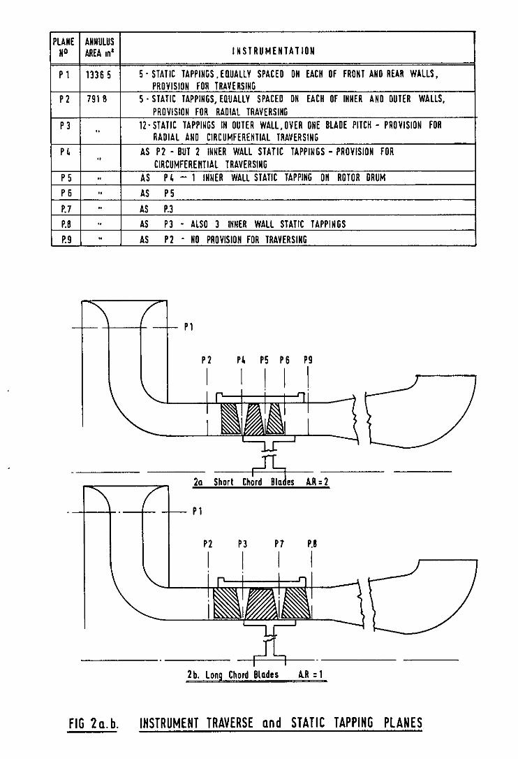
Five static pressure tappings were equally spaced around the circumference of the compressor inner and outer walls at several axial locations, Fig.2. Full radial and circumferential traversing over at least one blade pitch, Fig.3, is allowed by circumferential slots (5/E Ins. wide), cut in the stator casing.

2.3 Instrumentation and calibrations

In examining aspect ratio effects on axial-flow compressor performance experimentally, emphasis was centred upon the measurement of axial velocity profiles at the trailing edges of the blade rows, under a varie* of flow conditions. Such measurements must be carried out within the smell axial clearance, normally less than 0.500 ins, between neighbouring blade rows. This requFred an instrument small in dimensions but robust in construction, reading yaw angle, total and static pressures simultaneously. Such requirements were satisfied by a combination probe of the wedge type (Plate II and Fig.4). The accuracy of this type of instrument is discussed in Ref.8.

Fig.4 shows the wedge probe detail.

Calibration of the wedge for total head was carried out in the working section of a low speed, large cascade wind tunnel that could provide flow speeds up to 70 feet per second. Dynamic head readings from the wedge, set at its reference angle, were then compared with the true readings obtained from an NPL pitot-static Instrument placed in the vicinity of the wedge. The ratio of the true dynamic head to actual dynamic head reading then gives the total head calibration factor. Fig.5 shows the calibration curve.

A check on the turbulence level effects on the total head and yaw readings recorded by the wedge was obtained by placing various turbulence grids, generating turbulences in the free stream varying from 0.5s to IO& upstream of the working section of the wind tunnel. The results, which id.cate no effect of turbulence, are shown in Fig.5

The compressor rotational speed was recorded via a voltage pulse generator driven by the eddy current coupling shaft, and connected to an Avo-meter functioning as a voltmeter. The Avo-meter was calibrated against a rebolution counter over the whole speed range of the compressor.

Al.1 the pressures recorded by the instruments or by the wall tappings were measured on an inclined multi-tube (alcohol) manometer.

3.1

-5-

3. ExmRmmr~ I~WESTIGATIONS*

3.1 Overall performance characteristics

AP Curve.9 of overall static pressure rise coefficient over811 versus

0 &P m U" flow coefficient 3 are shown in Fig.9, for each of the tee aspect ratios,

where b =*o

en3 q a are calculated from mean values of 10 circumferential wall static press& readings. The plot is shown for a wide range of flow coeffioients (from 1.2 to 0.4 of the numbers (Re = 1.9 x l@, 1.45 x 108,

design value), and for several Reynolds

1.16 x 108 for AR = 1). 0.07 x 108 for AR = 2~ Re = I.9 x Id,

At each Reynolds number the throttle was set fully open. It was then closed progressively to the stall point, considerable care being taken to obtain readings at the points just prior to stall, and immediately after stall. A sudden fall in the static pressure rise across the compressor occurred at. the onset of stall, and under such a condition it proved quite impossible to operate the compressor at an intermediate point. The stall onset lines are therefore shown dotted on Fig.9. The audible detection of stall ms confirmed by observation of oscillations of the fluid in the manometer tubes connected to the five circumferential static pressure wall Lappings.

When the throttle was opened progressively from stalled through to unstalled operation, it was apEKent that the behaviour on throttle opening was different from that for throttle closing since the static pressure rise for unstalled operation was different in each case. The operation line for throttle opening is also shown dotted on Fig.9.

3.2 Entry conditions

Using the wedge instrument, radial traverses were made at entry to the stage. Readings in the inner and outer wall boundary layer were taken at O.O25" intervals from the wall for the first 0.250 of an inch and then at 0.100" intervals for the next 0.750 of an inch. Mainstream readings were taken at 1" intervals. Axial velocity, inlet flow angle, static and total pressures thus obtained are shown plotted against radius on Figs.10 and II for aspect ratio 2 and 1 respectively. The flow coefficients at which these traverses were made are $ = 0.647, 0.527 and 0.427. The reason for choosing these values is given in the next section. For purposes of clarity only selected measurement points are shown plotted on Figs.10 and II.

Entry conditions and in particular the boundary layers at entry appear to be similar for both aspect ratios. The boundary layer thickness deduced from total pressure measurements was slightly greater at. the cuter annulus wall. than at the inner annulus wall for both cases.

3.3/

* The compressor stage with aspect ratio 1 blades and that with aspect ratio 2 blades is hereafter referred to as compressor I and compressor 2 respectively.

-6-

3.3 Blade row traverses

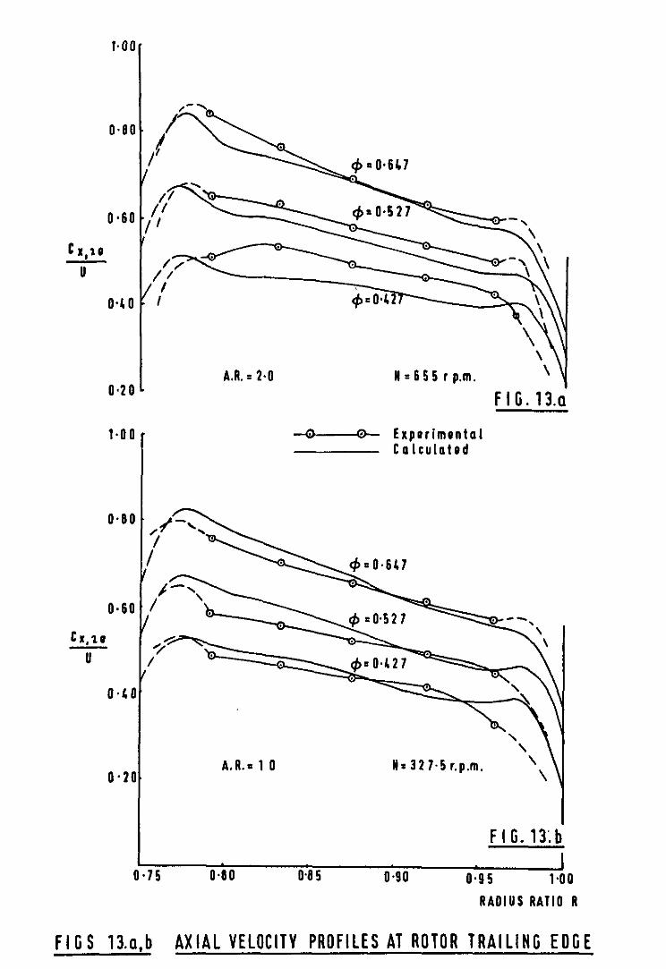
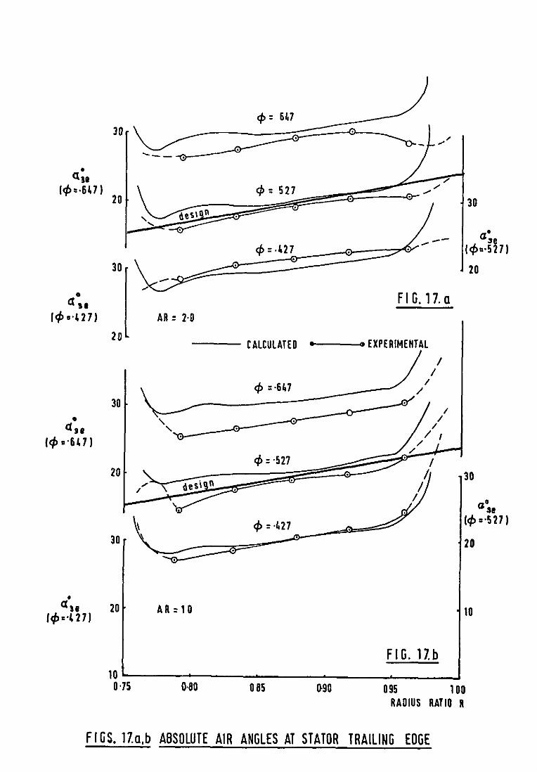
Using the wedge instmnent, circumferent.iaJ. traverses over one blade pitch, at I" intervals along the blade height and behind each blade row were conducted. Trailing edge mean values of axial velocity, outlet flow angle, etstic pressure and total pressure loss coefficient calculated from these circumferential measurements are shown plotted against radius* for three flow coefficients ($J =+0.647, 0.527, 0.427) and for each aspect ratio on Figs.12 to 22. The dotted lines on Figs.12 to 17 represent readings obtained in the end wall boundary layer where high accuracy cannot be expected.

The choice of the three flow coefficients at which all traverses have been carried out was based on the consideration that much of the unstalled mass flow range is bounded by the highest and lowest flow coefficients. The highest flow coefficient, $ = 0.647, represented a condition where incidences are negative and. compressor loadings are low. The second flow coefficient, + = 0.527, represented design conditions where incidenoes are near nominal and total pressure losses are minimum. The lowest flow coefficient, 6 = 0.427, represented near-stall conditions.

Although the lowest flow condition, q5 = 0.427, may not be as "near to stall" for compressor 1 as for compressor 2 , it was thought logical to test both compressors at the same value of flow coefficient.

3.4 Total pressure traverses

The measurement of total pressure may, in general, be regarded as more reliable than that of static pressure and yaw angle. In order that this measurement might be carried out in the boundary layer region near the annulus walls, the wedge instrument, functjoning as a pitot tube, was used. The other function of the wedge instrument, namely flow direction measurement, was also employed but only in an approximate wayaL so as to ensure that the wedge pitot tube was directed towards the flow to within 25'.

The total pressure measurements are presented on a non-dimensional basis and in contour form in Figs.23 to 28 for values of @ of 0.527 and 0.427.

3.5 Comparison with calculated results

Full calculations of the flow, including allowances for profile and secondary losses and changes in angles due to secondary flow were made for both compressors I and 2 for values of flow coefficient corresponding to the experimental results.

Details of these calculations are given in Appendix B.

The results of the calculations are compared with corresponding experimental measurements in Figs.12 to 17.

4./

* The method of calculation of experimental results is given in Ref.5.

** The normal manner in which the flow total head and direction is measured by the wedge instrument is to rotate the instrument until the readings recorded by the two wedge static holes sre exactly equal.

-7-

4. DISCUSSION

4.1 Overall characteristics

The overall characteristios for the oompressors 1 and 2,(Fig.9) show quite clearly that compressor I has a superior unstalled mass flow range. It also has a superior peak pressure rise. A close study of the two performance curves shows that the lncrease in range and static Pressure rise is quite substantial. The increase is approximately 1% for the former and 1C$ for the latter.

At flow coefficients higher than design (i.e., at I$ > 0.527), the performance of both compressors appears to be identical. At flow coefficients lower than design differences in performance may be seen to increase and just before stall these differences became maximum.

It is of interest to note that as the flow ooefficiept decreases, the compressor 1 performance curve levels off as it reaches the peak and then drops a little before it finally goes into stall. The compressor 2 performance curve, on the other hand, appears to reach its peak and then goes into stall just before it levels off. This suggests that compressor 1 approaches stall more stably than compressor 2.

In the stall region, static pressure readings recorded on the alcohol manometer oscillate so that these readings cannot be considered acourate. However, the two compressors exhibit hysteresis loops of the same general shape, the loop for oompressor I being the larger of the two. The static pressure rise in the stall region for compressor 1 appears to maintain the superiority over the static pressure rise for compressor 2, exhibited prior to stall.

No noticeable Reynolds number effects can be observed on either curve.

4.2 Axial velocity profiles in the mainstream

The axial velocity profiles behind any one blade row of compressor 1 do not show any appreoiable difference from the profiles behind the corresponding blade row of compressor 2, Figs.12, 13 and 14. This seems partiaularly true at the design and higher than design flow coefficients (i.e., $ = 0.527 and 0.647). At the low flow coefficient, Cp = 0.427, slight differences between compressor I and 2 mainstream axial velocities may be detected, the values for compressor I being the lower of the two. This Implies thicker annulus wall boundary layers for compressor 2.

4.3 Air outlet angles

The air outlet angles at the trailing edge of i.g.v., rotor and stator blade rows are shown on Figs.15, 16 and 17 for both compressbrs I and 2.

No appreciable differences in the meinstream values of outlet angle between compressor I and 2 can be observed. Angle measurements in the flow regions near the annulus walls ere shown as a dotted line.

4.4 Static pressures

The static pressures at the trailing edges of i.g.v., rotor and stator, shown on Figs.18, 19 and 20 for both compressors 1 and 2 do not show any conclusive differences. (Th e accuracy of the mainstream measurements is checked against a static wall tapping reading at each flow coefficient investigated. The results show that the agreement between the static Pressures recorded by the wedge instrument and by the wall taPPing is quite good*)

4.5/

-a-

4.5 Total pressure losses

The relative total pressure loss coefficient for the rotor of compressor 2 shows a considerable difference from that for the compressor 1 rotor, Fig.21. This difference appears as an increase in the loss coefficient near the root section for compressor 2, as the flow coefficient j.s decreased, no such increase being observed for compressor I. This seems to suggest that stall is taking place in the region near the inner annulus wall, (i.e., the regjon where the rotor blade meets the jnner annulus wall), for compressor 2, but not for compressor I.

At $I = 0.667 and 0.527, the absolute total pressure loss coeffioient is very much the same across the stator of compressor 1 and 2, Fig.22. At # = 0.427, the stator of compressor 2 shows clearly a region of high loss extending from the inner annulus wall to mid-span. The stator of compressor 1, on the other hand, shows that this loss is more confined to the annulus wall region. This suggests that at this low flow coefficient, the stator of compressor 2 is suffering from stall over the lower part of its span whilst the ststor of compressor 1 is suffering from a much less spread stall.

4.6 Total pressure contours

As a result of the somewhat inconclusive differenoes shown in the results of the experimental investigations discussed in the previous sections, it became evident that if a~ conolusions on the effect of aspect ratio were to be drawn, traverses extending in the annulus wall boundary layer had to be undertaken.

Complete total pressure contours at exit from the three blade rows are shown for compressors i and 2 operating under design ($ = 0.527) and off-design conditions (# = 0.427), on Figs.23 to 28.

At the trailing edge of the i.g.v. blade row the waviness of the "mid-wake" line at the low floe condition for compressor 2 indicates that secondary flow is stronger in compressor 2 than compressor I, althou& the boundary layer thickness on tKe annulus walls for both flow conditions appears to be much the same for both aspect ratios.

The total pressure contours measured behind the rotor blade row are experimental mean values of the true time-varying quantities. A very high degree of accuracy is therefore not to be expected, but nevertheless the results, Figs.2l+ and 27, exbibit significant features and show some particular differences between the tvo compressors.

At 6 = 0.527, the general level of total pressure at this section is slightly hi&er in compressor 1 than in compressor 2. At $ = 0.427, this difference is accentuated and the results for both compressors indicate regions of higher total pressure at the extreme ends of the blade span. However, the trough in total pressure over the part of the blade near the hub is nuch more marked for compressor 2 than for compressor 1.

The explanation of these results is not easy to find. The measurements of relative air angles, Flg.16, do not extend into the root region in which the higher values of total pressure are observed. The higher values may be associated with over-turting at the root, or with an increase in work done as a result of reduced axial velocity in the end wall boundary layers.

Certainly there are marked differences between the total pressure distributions downstream of the two rotors but the present experimental measurements are not sufficiently detailed to indicate the oause of the difference. The/

-9-

The total pressure contours at the trnlling edge of the stator blade row also show substantial differences between compressors I and 2. At # = 0.527, the annulus wall boundary layer thickness is evsdently thicker for compressor 2 than for compressor 1, although the boundary layer thicknesses on the suction surface of the blades in the mainstream is very much the same for both compressors. At $ = 0.427, major differences are apparent, complete wall stall occurring in compressor 2, particularly at the hub, but not in compressor I. This result reflects the total pressure loss coefficient results obtained for the stator, Fig.22, and may result from variation of incidence on to the stator blades associated with the total pressure distribution at the rotor outlet.

4.7 Flow calculation with losses

Actuator disc calculations (including losses) of the trailing edge axial velocity profiles, Figs.12, 13 and 14, show good agreement with experiment over most of the blade height. In general, my disagreement appears to be in the regions near the inner and outer annulus walls. Neither the losses nor the outlet angles, Figs.15, 16 and 17, near the annulus walls can be estimated with sufficient accuracy.

There are two factors that may be considered responsible for incorrectly estimating the profiles near the annulus walls. First, the use of cascade loss data is open to question, as may be seen by comparing the curves of Fig.8 (the loss distributions used in the calculations) with those of Figs.21 and 22 (the loss distributions actually measured).

In spite of these disparities, the use of cascade data in expressing the loss for the middle part of a blade operating near its design conditions, results in a reasonably accurate prediction of performance, but even the inclusion of distributed secondary and clearance losses, as in the present calculation, does not lead to very good estimates of the flow at the annulus walls.

Secondly, the assumptions made on the size and growth of the annulus wall boundary layer areorltxal in the loss and angle calculations. The thickness of the boundary layers at root and tip that were aotudly used in the loss calculations were deduced from early traverses at the tip section and were approximately one inch. The entry velocity profile assumed for the calculations is shown on Fig.6 together with the measured profile. It is evident from Fig.6 that the profile assumed for the calculation at the inner annulus wall is substantially in error, and the calculation of the profiles at the inner wall is invalidated.

5. CONCLUSIONS

5.1 The overall performance characterxstics have shown that the range of uhstalled operation for compressor 1 is wider than that for compressor 2. At flow coefficients higher than design, the performance of both compressors appears to be identical. At flow coefficients lower than design, differences in performance appear, with compressor 1 achieving the higher overall static pressure rise. Stall with compressor 2 seems to occur suddenly whilst it is gradual with compressor I.

5.2 The traverse results show that the three-dimensional mainstream flow is substantially the same for both compressors, thus confirming the inviscid calculations of kef.6.

5.3/

- 10 -

5.3 The mn~or cause of the difference in the overall performance of the two compressors appears to be the marked differences between the total pressure distributions drvnstream of the mtor at the same (naar-stall) flow coefficient. In addition, there is severe stator wall stall in compressor 2, compared with very little stntor wall. stall in compressor I.

5.4 Since no appreciable difference in the values of trailing edge axial velocity and outlet air angle has been observed between compressors 1 and 2, ft is concluded that the work done by both compressors over the whole flow range is substantially the same.

5.5 Comparison of the actuator diso "loss" calculations with experimental results, Ref.5, shows that while some improvement on inviscid calculations is achieved, the velocity proflles, particularly at the hub and the annulus walls still cannot be predicted accurately. This is due to the inadequacy of the loss data and poor estimates of annulus wall boundary layer thickness.

ACKNCjlLEDGEK!,Wl'S

The author wishes to express his gratitude to Professor J. H. Horlock for the @dance under which this work was carried out, and to Professor J. F. Norbury for editing the manuscript.

APPENDIXA/

- 11 -

APF'ENDIXA

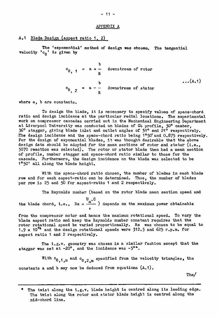
A.1 Blade Design (aspect ratio 1. 2)

The 'exponential' method of design was chosen. The tangential velocity 'ce' is given by

b CBS f = a+R

downstream of rotor

b

08s2 = "-ii downstream of stator

. ..(A.i)

where a, b are constants.

TO design the blade, it is necessary to specify values of space-chord ratio and design incidence at the particular radial locations. The experimental work on compressor cascades carried out in the Mechanical Engineering Department at Liverpool University was conducted on blades of C4 profile, 30" camber, 36O stagger, giving blade inlet and outlet angles of 51° and 21° respectively. #The design incidence and the space-chord ratio being l"5O'and 0.875 respectively. For the design of exponential blades, it was thought desirable that the above design data should be adopted for the mean sections of rotor and stator (i.e., 5070 reaotion was selected). The rotor or stator blade then had a mean seotion of profile, camber stagger and space-chord ratio similar to those for the cascade. Furthermore, the design incidence on the blade was selected to be lo50 all along the blade height.

With the space-chord ratio chosen, the number of blades in each blade row and for each aspect-ratio can be determined. Thus, the number of blades per row is 25 and 50 for aspect-ratio I and 2 respectively.

The Reynolds number (bLsed on the rotor blade mean section speed and

u,.c the blade chord, i.e., Re = - ) depends on the maximum power obtainable

" from the compressor motor and hence the maximum rotational speed. To VW the blade aspect ratio and keep the Reynolds number constant requires that the rotor rotational speed be varied proportionally. 1.9 x 10%

Re was chosen to be equal to and the design rotational speeds were 312.5 and 625 r.p.m. for

aspect ratio 1 and 2 respectively.

The i.g.v. geometry was chosen in a similar fashion except that the stagger v7as set at -20°, and the incidence was -5O*.

With %,l,m and 'fj,2,m specified from the velocity triangles, the

oonstants a and b may now be deduced from equations (A.l). The/

l The twist along the i.g.v. blade height is centred along its leading edge. The twist along the rotor and stator blade height is centred along the mid-chord line.

- 12 -

The air angle distributions with radius may then be obtained by considering the radial equilibrium equations at the design point, where there are no gradients of stagnation enthalpy, i.e., equal work being done at all radii, thus,

do ce d 0 -25 + - . - (t-.0& = 0 Xar r d.r

. ..(A.2)

Integrating equation (A.2) with respect to r, we get

o= = constant - 2aa. x log, R + b/d (1 - R) . ..(A.3)

where the constant is determined by satisfying the continuity condition.

Using the actuator disc theory these "infinity" axial velocities obtained from eqn. (A.J), may be modified to give the Leading and trailing edge values by allowing for the interference effects of the adjacent blade rows.

With the blade axial spacing, the blade chordal dimension and the hub-tip ratio of the compressor all specified, each blade row may then be replaced b a hypothetical actuator disc located at the bLade centre line (mid-chord 3 , Ref.9.

The trailing edge axial velocities could now be calculated from interference equations of the form

(ox i+, - ox ,I,” 0 0 - x,ie = x,i

+ 2 2 . ..(A.&)

allowing for interference effects from adjacent disc only, Ref.10.

The design air angles distribution with radius are then deduced from

b

tan ae = cB,i = a-E for a rotor 0

x,le 0

x,le

tan p, = u - Oe,1 U - (a + g) = for a stator

0 x,le 0 x,le

. ..(A.5)

Ref.11 gives detailed application of aotuator disc theory to design of axial compressors.

Blade angles, camber and stagger at various radial positions may now be computed for a blade that will produce such air angle distributions. This computation follows an iterative procedure whereby deviation rules and other empirical cascade data for deflection are employed, Ref.12. Such a procedure is lengthy and a computer programme was devised for the purpose of speeding up the calculations.

The/

- 13 -

The final step of blade design, once a profile shape is decided upon, is the computation of the blade surface co-ordinates. These may be quickly and accurately obtained with the aid of a computer programme.

The use of the interference equations in the blade design procedure, results in aspect ratio 1 blade angles to differ by a maximum of two degrees from those.for aspect ratio 2. Depending on the manufacture accuracy, a differenoe of this order mey either be enlarged or reduced, and since such an accuracy was considered questionable, blade design values were the seme for both aspect ratios. Blade surface co-ordinates values for the low aspect ratio were twice those for the higher aspect ratio.

A.2 Desia geometry and other data

All the blades have simple cylindrical root platforms and threaded root fixings. When aw one set of blades is built in the compressor*, the axial spacing between any two neighbouring rows of blades was kept at a minimum of 0.90 inohes, to allow access of instrumentation in the space between the blade rows and to any radial location without risking damage to the instrument. Blade tip olearanoe was kept at 0.060 inches.

The pertinent design details for both blade designs are listed in Table I.

* Plates 3 and 4 show a representative set-up of the exponential blades.

- 14 -

AF'F'ENDMB

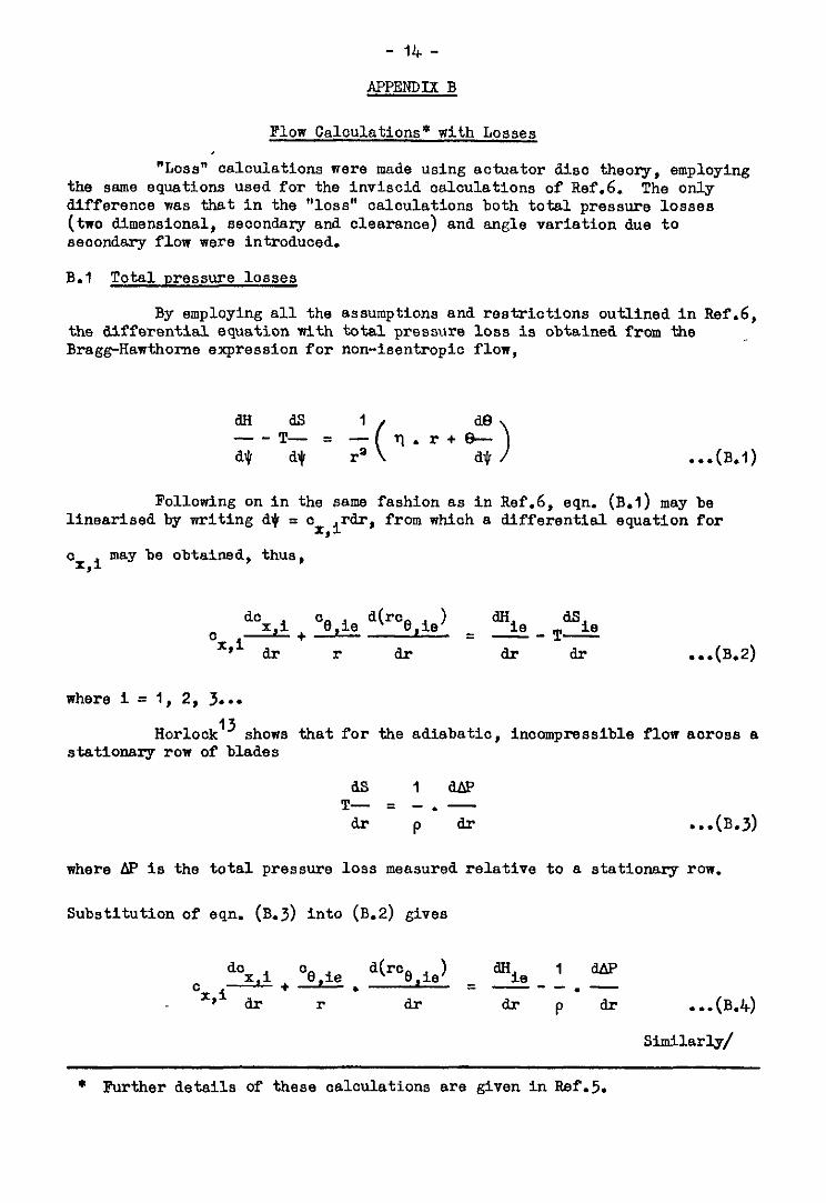
Flow Calculations* with Losses

"Loss" calculations were made using actuator disc theory, employing the same equations used for the inviscid oalculaticns of Ref.6. The only difference was that in the "loss" calculations both total pressure losses (two dimensional, secondary and clearance) and angle variation due to seocndary flow were introduced.

B.l Total nressure losses

By employing all the assumptions and restrioticns outlined in bf.6, the differential equatibn with total pressure loss is obtained from the _ BraggHawthcrne expression for non-isentropic flow,

aH ds I de --T- = - q.r+f3- a$ a* r= ( a* > . ..(B.l)

Following on in the same fashion as in Ref.6, eqn. (B.1) may be linearised by writing d$ = ox i Mr, from which a differential equation for

f c

6 may be obtained, thus,

da

J4 + %,ie G-c )

c x,i 0,i.e = se *I%. ar r ar al- ar . ..(B.2)

where I = I, 2, 3...

Hcrlock13 shows that for the adiabatic, incompressible flow aorcss a statlonarg row of blades

as ldhp T- = -*-

h- P lb . ..(B.j)

where AP is the total pressure loss measured relative to a statics row.

Substitution of eqn. (B.3) into (B.2) gives

c i,l 0,111 cI,I!.S~ hi

+ . = ?L%l.iE al- r ar al- P ck . ..(B.4)

Similarly/

* Further details of these calaulaticns are given in Ref.5

- 15 -

Slmllarly for a rotating blade row, with

as 1 aAP' T- = -,-

al- P -3.r . ..(B.5)

where AP' is the tota& pressure loss measured relative to a moving IT)W.

B.l.1 Sldn friction losses on blade surfaces

The effect of skin friction on the blade surface is to cause irreversibilities in the flow, leading to an increase in entropy and loss in total pressure across the blade row.

The total pressure loss arising from skin friction on the blade surfaces may be based on Lieblein's low-speed relationship between the equivalent diffusion (Deq) and the wake momentum-thickness parameter (Wmt), at any flow condition. This relationship, for a compressor with parallel wall annulus is

D S.C02pin c x out

= eq [

K;I +Xa(i-i*)Ks +& . c * (

tan Pin - c ' - tan Pout >I x x,in

x cos Pout %,in . cos bl %,out . ..(B.6)

and can be applied to rotors and stators. &, Ka, Ks and X, are constants.

Using Swan's statistical curve fit for rotors, Fig.7, a value for the wake-momentum thickness Wmt rt may be obtained. Similarly, using Lieblein's

experimental curve, given .ss inAependent of radial location, Fig.7, for the variation of D with W

w mt for C& circular-arc blades at and off minimum loss

conditions, a value for Wmt 9

st may be obtained.

The approximate expression for W,,,t then gives the required total

pressure loss coefficient, thus,

u 2c, wmt of =

S*COS Bout

( 11; p,,=

ou

where

(%r)st u of = 1 for a stator

&in

u (%f)rt of =

sptia for a rotor

. ..(B.7)

. ..(B.8)

. ..(B.9)

The/

- 16 -

The inlet guide ve ea skin friction loss is baaed on Ainley's nozzle blades minimum profile loss tE and its tote1 pressure loss coefficient is defined as

u (%f)igv cf = 1

2pC=oUt . ..(B.lO)

B.l.2 Tip clearance flow losses

The total pressure 1 aa arising from tip olearence flow is obtained from .e formula given by Vavra 15 for the tip clearance drag coeffioient. Vavra, using .e flow model devised by Reins, derived the following formular

to

'Dt = 0.29 . CL# . - L . ..(B.il)

where to is the tip olesrence.

The drag coefficient for e oompreaaor oaaoade is related to the total pressure loss ooefficient; thus,

c . a ooa3a

cD = c'---- COS%in

and for an igv or turbine cascade thus,

c .a CO&i

cD = -7~ coa aout

. ..(B.12)

. ..(B.13)

tan ain + tan a where z = arc tan out .

2 >

By combining eqna. (B.11) end (B.12) we have for a oompreaaor oeaoade

to c Et

J, = 0.29 . CL ooaaain

. - . - . L a OOS’;; . ..(B.l4)

and by combining eqna. (B.11) and (B.IJ), we have for .e compressor aaacede

tc c

= 0.29 . CL% . - . - . ooaaa

et out

L a 00s";; . ..(B.15)

B.1.3/

- 17 -

B.i.3 Cascade secondrrry flow losses

Vnvro's cmpiricnl xlnt.ion for the induced drnC coefficient due to :~ocond::ry flow i:; used. This rol:ltwn 13

. ..(B.16)

By combining eqns. (F.12) and B.l6), we have for u conpressor cascudc,

c CL2 c

= 0.04 . - . - . COS%in

cs AR 3 COS?Fi . ..(B.17)

Similarly, for a turbine cascade,

c CL’ c

= 0.04 . - * - . oos2aout

cs AR s CO2;;i . ..(B.l8)

The drag coefficients CDt and CDcs ~lven by eqns. (B.11) and (B.16)

respectively are energy averaged over the whole blade length. The dorlved pressure 1033 coefficients Zt and Zcs will also be averaged in the same way. In order that these coefficients may be used for a particular blade element, new coefficients at, cr cs' referred to these elements, must be calculated,

where u 3naa (B.9) an: (B.10::

are each defined in a sirmlar way as cof in eqns. (B.8), Such a calculation is detailed in Ref.5; essentially

the loss is assumad to vary parabolically from zero at the edgo of the boundary layer to a maximum at tl e wall. The integral of this local loss IS equal to l.ho "Vovra" overall loss. The thickness of the boundary layer is assumed to remain constant throuf;h the compressor at the entry value.

B.1.4 Equntlons with total pressure loss

The cquatlon with total pressure loss is obtained by substxt.utinC eqns. (A.4) and (R.5) into eqn. (B.4), it being assumed that an overall total pressure loss ooefficlent may be def'lned for the reClon outside the boundary lnyer an

u = IT- cf . ..(V.lQ!

and for the region within the boundav layer* ns

6=u cf + 61 + UC3 . . . (E.?O)

For the case of the single-stage compressor, eqn. (B.4) in its new form may be applied across each blade row. Three sirmtltancous differential equations (including total pressure loss) for the "infinity" distributions of axial velocity, arp thus obtained.

Id

* In the region where there is no tip clearance, at = 0.

- 18 -

In non-dimensional form these equations become:

b,, V, + b,2 V2 + b,3 V3 + E, = 0

b2, V, + b22V2 + b23 V3 + E2 = 0

b>, V, + b32 V2 + bf3V3 t ES = 0 ..,(B.21)

where

and bjk' j E my be functions of R, o =, j9 tan (ae or P,),

A complete statement of eqn. (B.21) is given in Ref.5, Fig.8, shows a distribution of the calculated total pressure loss coefficients with radius for the i.g.v., rotor and stator blade rows.

B.2 Outlet .angle variation due to secondary flows

The tracing of the secondary vorticities through a single-stage compressor is detailed in Refs.5 and 16. With the streamwise vortioity components at exit from each row determined, the induced aeoondary velocities and the associated changes in outlet air anglee is then calculated from Hawthorne's series s6lution. For this solution, Hawthorne ‘7 has shown that series terms with n > 1 ay small and therefore may be neglected.

) If the streamwise vorticity at exit from B two-dimensional casoade of the same geometry as the tip section is c,(z), where E is the distance from the wall, then the mean change of outlet angle across the blade pitch at a point Z from the wall ie given for o < 2 < 6 by

cos h : (L - Z) Z xz TJ.4

sin h v I

c;,(z) sin h - dz 0 Y 1 . ..(B.22)

- 19 -

and for z > 6 by

tan ( haout ) = x2:x,e . coss;n'h'; ') "i S,(z) sin h ; dz . ..(B.23) 0

where y = s . oos (I out'

If the radial distribution of outlet angle based on two-dimensional cascade data is aout( then the distribution corrected for the secondary flow is gLven by

%ut(o) b-1 = aout + ~outw . ..(B.24) where Aawt(rt - r) is assumed to be the same as Aa,-&Z), the two-dimensional calculation.

B.3 Calculation procedure

For the single-stage compressor, eqns. (B-21) are to be solved simultaneously. the method of solution is outlined in Ref.6.

To solve eqns. (B.21), an estimate of the radial distribution of the total pressure loss ooeffxients and the outlet air angles for each blade row is required. Such an estimate is obtained as follows:

(a) Obtain the "infinity" and "trailing edge" distributions of axial velocity from a solution to eqns. (B.21) with the total pressure loss coefficients made equal to zero and the outlet air angles taken to be those at design (the three-dimensional, inviscid solution, Ref.6).

(b) Assume a velocity profile at entry ta the aompressor stage oonsisting of n th power law &Lstribution in the inner and outer wall boundary layer and a uniform distribution outside it, Ref.6.

(c) Calculate the entry vorticity and then trace the secondary vorticities through the compressor stage using the design outlet air angles, Ref.16.

(d) For each blade row

(i) Caloulate the change in the air outlet angle duo,,(r) from eqns. (B-22) and (B.23) using cx s,(r) obtained in (a) and Es(r) obtained in (c). '

(ii) Obtain the new distribution of air outlet angle aout(o)(r) corrected for the secondary flow from (B.24).

(iii) Calculate u(r) using cx,e(r) obtained in (a) and the design outlet air angles.

(8) /

- 20 -

(8) Re-solve eqns. (B.21) with estimates for a(r) from d(iii) and for aoutCcl(r) from d(U)* to obtain a new distribution of "infinity"

and ';tkling edge" axial velocity.

(f) Re-trace the seoonaary vorticity usin the same entry velocity profile assumed in (b) and a out(o)(rf obtained in d(ii).

(g) Re-calculate AaoUt( ) r and a(r) for each blade row using cx e(r) obtained in (e), &s(r) obtained in (f) and haout obk.ned in d(U) , and use these as new estimates in the next approximation.

(h) Repeat steps (e), (f) and (g), until no further change in the c x e distribution for each row is obtained.

f

APPENDIX c/

* Horlocki6 has shown that the use in an actuator disc analysis of the exit air angle as calculated from eqns. (B.22) and (B-23) is justified, the streamwise vortlcity being apprcxlmately the same at exit from the row of widely spaced blades and the equivalent actuator disc.

- 21 -

AlTmDIX c

R

U

09 w

C

X

L

h, H

PI p

AP, AP'

I:

u

cD

RZ

AR

K

h

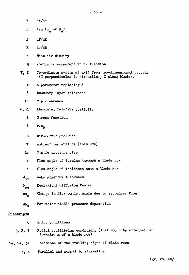
NCTATION

Velocity components in r, 8, x co-ordinates system

Dimensionless radius (= r/rt)

Absolute flow angle at entry or exit from 8 stotor row measured from the x-direction

Relative flow angle at entry or exit from a rotor row measured from the x-duection

Angular velocity

Blade speed (= nr)

Absolute, relative velocity

Chord length

Distance from actuator disc (always positive)

Blade length (= rt - rh)

Static, total enthelpy

Static, total Pressure

Absolute, relative total pressure loss

Total pressure loss coefficient integrated over the blade length

Total pressure loss coefficient referred to a blade element

Two-dimensional dreg coefficient

Reynolds number (= urn"' ' )

Entropy

Blade spacing

s.00~ (oe or p,)

Flow coefficient (= o,,/U,)

Aspect ratio (= L/C)

Constant (= rb,)

cX,$cX,O

- 22 -

v

f

F

X

P

rl

y, 28

z

s

to

E;, r

$

e

B

T

AP

E

i

W mt

D eq

Aae

Subscripts

0

I, 2, 3

le, 29, 3e

99 n

Mean air density

Vorticity component in O-direction

Co-ordinate system at exit from two-dimensional cascade (Y perpendicular to streamline, 2 along blade).

A parameter replacing 2

Boundary layer thickness

Tip clearance

Absolute, relative vorticity

Stream function

lr.0 e

Barometric pressure

Ambient temperature (absolute)

Static pressure rise

Flow angle of turning through a blade row

Flow angle of incidence onto a blade row

Wake momentum thickness

Equivalent Uffusion factor

Change in flow outlet angle due to secondary flow

Manometer static pressure depression

Entry conditions

Radial equilibrium conditions (that would be attained far downstream of a blade row)

Positions of the trailing edges of blade rows

Parallel and normal to streamline

igv, rt, st

sf

to

OS

t, m, h

in, out

max

I

T

6

Superscripts

I

- 23 -

Pertaining to inlet guide vme, rotor and stator respectively

Due to skin friction

Due to tip clearance

Due ta oascade secondary flow

Tip, mean and hub respeotively

At inlet to and outlet from a blade row

Maximum

Indicated

TX-U.3

Gauge (i.e., relative to atmospherio pressure)

Mean Value

Relative to a row

REFERENCES/

Footnote: Wherever two or more subscripts era used together, a comma has been used to separate them; e.g., ox is written 0 .

0 X,O,lWX

Title. etc.

Reynolds number effects in cascades and axial-flow compressors. Trans. A.S.M.E., Series A, 86, 236. (1964)

No. Author(s)

1 J. H. Horlock R. Shew D. Pollard A. K. Lewkowioz

2 D. Pollard

3 M. R. A. Shaelen

4 J. A. Fligg, Jr.

J5 G. J. Fahmi

6 J. H. Horlock G. J. Fahmi

7 R. Shsw A. K. Lewkcwice

8 J. H. Horlock

9 J. H. Horlock E. C. Deverson

IO J. H. Horlock

/II A. D. Carmichael J. H. Hcrlook

12 A. R. Howell

13 J. H. Horlock

The low speed perf'ormanoe of two-dimensional oascade3 of nerofoil. Ph. D. Thesis, Liverpool Universitg. (1964)

The stalling performance of cascades of different aspect ratios. Ph. D. Thesis, Liverpool University. (1967)

Tests of 8 low-speed three-stage axial flow compressor at aspect ratios of one, two and four. AIAA Paper No. 66-613. (1966)

The effect of blade aspect ratio on the performance of axial flow compressors. Ph. D. Thesis, Liverpool University. (1967)

A theoretical investigation of the effect of aspect ratio on axial-flow compressor performance. ARC C.P. Nc.943. (1966)

The construction and testing of a large axial-flow compressor. ARC C.P. No.62Q. (1962)

Instrumentation used in measurement of the three-dimensional flow in *n axial-flow compressor. ARC C.P. No.321. (1955)

An experiment to detennlne the position of an equivalent actuator disc replacing a blade row of a turbomachine. ARC.C.P. No.426. (1958)

Communication relating to the paper "Three- dimensional design of multi-stage axial flow compressors" by J. 17. Railly. J. Mech. Eng. Soi. 2, No. 3, 286. (1961)

Actuator disc theories applied to the design of axial-flow compressors. ARC C.P. No.315 (1956)

The present basis of axial-flow compressor design. ARC R.& M.2095. (1942)

Axial-flow compressors - fluid mechanics and thermodynamics. Butterworths, London. (1958)

- 25-

Title, etc.

Losses and effioiences in axial-flow turbines. Int. J. Mech. Sci. &, 1, 48-75. (1960)

Aero-thermodynamics of fluid flow in turbomachinery.

-John Wiley, New York. (1960)

Annulus wall boundary layers in axial ccmpresscr stages. J. Basic Brig., 85, D, I, s-61. (1963)

Some formulae for the calculation of seconderg flow in cascades. A.R.C.17 519. (1955)

5. Author(s1

Jl4 J. H. Horlook

Jf5 M. H. Vavra

16 J. H. Horlock

17 8. R. Hawthorne

BW

SIISLE STASE OUTLET THPOlllE FIPFIIYFITAI

I I II L h III IIIII II

- * II

VOLTASE PULSE SEIEIIIITOR

FIG 1. DIAGRAMATIC LAYOUT OF RIG

a’ AS P3 - ALSO 3 INHER WALL STATIC TAPPINGS p.9 1 ” AS P2 - NO PROVISION FOR TRAVERSING

- Pl

P; P; P; 1; P,

1 I

.-

2a Short Ch;rd glades AR=2

- Pl

‘I’ 9’ 9’ / I

Tc/ Tl -

2b. Long Chord Blades AR ~1

FIG 2a.b. INSTRUMENT TRAVERSE and STATIC TAPPING PLANES

---.

r --

FlG.3. CIRCUMFERENTIAL PLANES OF TRAVERSE

.ObO” o.d. pitot

ENLARGED SECTION A-A

FlG.f,. WEDGE PROBE DETAIL

1 b 6 6 10 PI - p, tnr maths on 5’bb’

inclined manometer.

I 30 16

c FtJsrc.

FIG. 5. WEDGE INSTRUMENT CALIBRATION CURVE

cx,o Urn

06

cx.0 Urn

0.b

. .? a MEASUREU PROFILE

CALCULATED PROFILE (Appendix E 1

----- INVISCID CALCULATION

I AR : 2.0

III I * 655 r.p.m.

,

Urn

FIG. 6a

- MEASURE0 PROFILE

CALCULATED PROFILE (Appendlx E 1

---- IHVISCIO CALCULATION

AN = 1.0 N427.5 r.p.m.

III III II II

-- 7

030 0.85 0.90 0.95 1.00 RADIUS RATIO R

FIG. 6 b

:;,o,max.

Urn

FIG. 6a,b THE ENTRY VELOCITY PROFILE

.5 c1

‘1 \ \ \ \ \ \ \

\ \ \

\ \

\ \

\ \

\ \

\ \

\ \ c

\

\ \

\ I \ \ \ L \ \ \

\

I- I

% % ;c z . .

m m ;i; CI -’ + i *

ROTOR AND STATOA LOSS ESTIMATION CURVES FIG. 7

OOL

uigv

OK?

0

I \ \

--- AR.l.0 c#as o-527 :

(FIRST LOSS CALCULATION)

\ I

0.75 060 085 0.90 0.95 1.00 RAOIUS RATIO R

FIG. 8 RADIAL OISTRIEIUTION OF OVERALL TOTAL PRESSURE LOSS COEFFICIENT

.

FIG. 9 OVERALL CHARACTERISTICS OF THE VARIOUS COMPRESSOR BUILOS

0.2 0 1 2 3 4 5 6

FIG.10 r-rhins 0. 1 2 3 4 5 6

FIG. 10b r-rh ins

r-rhlns. - 0.21 I 0 1 2 3 I 5 6

FIG. ?Oc r-rk ins

FIG. 10d

d i

0’ - Y

” &

” 0 - LL

FIG.11. CONDITIONS AT ENTRY TO COMPRESSOR STAGE (A.R.= 1.0)

A.R.8 2-O I = 6 5 5 r.o.m . 0.201 I

FIG. 12.a

Experimental Calculated

A.R.: 1.0 H = 327.5 r.p.m.

II.75 040 045 0.90

F I G. 12.b

I 0.95 140

RADIUS RATIO R

FIGS. 12.a,b AXIAL VELOCITY PROFILES AT I.G.V.TRAILING EDGE

AA = 2.0 H=655 rp.m.

FIG. 13.a h r;\ Experimental

Calculated

A.R.n 10 Ws 321.5 r.p.m.

75 040 0.8 5 0.90 I

o-95 1.00

AAOIUS RATIO II

FIGS 13.a,b AXIAL VELOCITV PROFILES AT ROTOR TRAILING EOGE

1.00 c

A.A = 2.0 I = 655 r.p.m FIG.14.a

6 ExperimentaL Calculated

A II = 1-O II-327~5 r.p.m.

FIG.14.b

0.7 5 O-80 04 5 0.90 0.95 1.00 RAOIUS RATIO R

FIGS.14.aab AXIAL VELOCITY PROFILES AT STATOR TRAILING EDGE

4, IQ, 427)

AR-20 FIG. 15.a

20 1

- EXPERIMENTAL CALCULATE0

I /

I c

075

FIG 15.b .

095 100 RAOIIJS RAllO R

FIGS 15.a,b ABSOLUTE AIR ANGLES AT I.G.V. TRAILING EDGE

- EXPERIMENTAL

- CALCULATED

30

sse :c#~=527) 20

By- -.

20

10

FIG.16.b I

0.75 080 005 090 095 100 RAOIIJS RATIO R

!7I

FIGS. 16 a.b RELATIVE AIR ANGLES AT ROTOR TRAILING EDGE

14427J AR = 2.0

20 CALCULATE6 -EXPERIMENTAL

I / /I

10 6 0.75 040 065 090

FIG. 1Zb FIG. 1Zb

095 100 RAOIUS RATIO R

FIGS. ll.a,b ABSOLUTE AIR ANGLES AT STATOR TRAILING EDGE

0

-0.20.

db

-O*bOq~

plc,g 1/2PU’m

-0.60.

-0x90-

Q

A.R.n 2.0 N= 655 r.p.m.

FIG. 1e.a @ Static wall reading

AA. 1.0 N = 3 2 7.5 r.p.m.

p I a,9

J+Pu’m -0.60 *

FIG.18.b

FIGS. lB.a,b STATIC PRESSURES AT I.G.V. TRAILING EDGE

RAOIUS RATIO R

ple,9 II’IPU’m

-0.20

-0.60.

O.bO

0.20

lC,$ P l/?PU*m 0

- 0.20

-O.bO

A.R.a 1.0

FIG. 19 a

@ Static wall reading

A.R. I.0 Wn317~5r.pm.

0

FIG, 19.b

0.75 0.60 0.65 0.90 0.95 1.0 0 RADIUS RATIO R

FIGS. 19.a,b STATIC PRESSURES AT ROTOR TRAILING EDGE

O*kO - a

0.20 . 0

pa49 112 P U’m

0 -

-0.20 .

d>

-0.40

0.60

040

0.21

pseg l/2 P II’ m

0

-0*2(

A.R.n 2.0 II = 655 r.p.m.

FIG 20.a @ Static wall rtading

A R. 1.0 W 8 3 2 7.5 r.p.m. Q

FIG 20.b

15 .040 045 0.90 o-95 0 RADIUS RATIO R

FIGS 20.a,b STATIC PRESSURES AT STATOR TRAILING EDGE

0

FIG. 21.a

AR: IO

0.75 040 085 0.90 095 100 RAOIUS RATIO R.

FIG. 2T.b

FIG. 2l.a,b RELATIVE TOTAL PRESSURE LOSS COEFFICIENT ACROSS ROTOR

AP

‘pc’l

0

AP V2~c'rc

0.2-

I1 .

o-

.4

,

I _

0.2

II.1

0

AR:10

FIG. 22.a

075 040 045 090 cl*95 100 RAOIUS RATIO R FIG. 22. b

FIG. 22.a.b ABSOLUTE TOTAL PRESSURE LOSS COEFFICIENT ACROSS STATOR

,I SUCTION SURFACE .\ PRESSURE SUPfACE

WOW-OIMENSIOWAL BLADE PITCH

#ON-DINEHSIOHAL BLADE PllCli

FIGS. 23.a.b TOTAL PRESSURE CONTOURS AT I.G.V. TRAlLlNG EDGE (AT-DESIGN] ,

A R. 24 Isb55r.p.m

NON-OIMENSIOHAL BLAOE PllCN

FIG.24.b

FIGS 24 a,b TOTAL PRESSURE CONTOURS AT ROTOR TRAILING EOGE

-(AT-DESIGNI

PRESSURE SURFACE \ SUCTION SURFACE

PRESSURE SURFACE SUCTIOH SURFACE

I= 655cpm. a*527

MID-WAKE LIKE

CONTOURS OF& h P u’m

ARslO Wk327~5tp.m. c$8.521

FIG.25 b

FlGS.25a.b TOTAL PRESSURE CONTOURS AT STATOR TRAILING EOGE (AT-DESIGJI

SUCTIOW SURFACE PRESSURE SURFACE

AR: PO H:6551

NON-OIMEIISIUNAL BLADE PITCH FIG. 26.a

SUCTION SURFACE

PRESSURE SURFACE

-\ II ILMI~-WAKE LINE I

I p.m.

COWlOURS OF PO 04

112 p u’m AR=10 N-327.5r.pm

NOW-OIMENSIONAL ELAOE PITCH FIG. 26.b

FIGS 26 a.b TOTAL PRESSURE CONTOURS AT I.G.V. TRAILING EDGE

(OFF-DESIGN1

r-rh

NOW-0lMEilSIOHAL BLADE PITCH

o 5 - ’ --- r-Q ’ C0ll10URS OF -i- \ 04 -- /I .plo,g

NON-0lHEWSIOIAL BLADE PITCH

112 Pu'm ARzl.0 6=327~5rp.m

4)E421

FIG. 27. t!

FIGS 27.a b TOTAL PRESSURE CONTOURS AT ROTOR TRAILING EDGE

(OFF-OESIGNI

PRESSURE SUBFACE SUCTIOII SURFACE

HON- DIMENSIONAL BLAOE PITCH

I p.m.

PRESSURE SURFACE SUCTION SURFACE

AR=10 Nz327.5rp.m

NON-OIMENSIOWAL BLADE PITCH

FIGS 28a.b TOTAL PRESSURE CONTOURS AT STATOR TRAILING EDGE (OFF-OESIGN)

cc~llXLE1 ANGLEI cx;lOUlLEl bUGlEI e ICAMBER ANGLE1 A ~S~AGGEU AR~LEI

-

0 2

2 ::

2 2

751 - U7! -

005 - I751

I67! -

OO! - 115: -

ItBli -

00: -

z C

s zi 111 - 21

lb - 18 - 11 -

2b - 16 -

21 -

2b -

- z =

z u E z i2 2 -

ioo

-

6 00

-

6 00

-

DESIGII

COWSTAIIT

SECTIOX

BLAOE

0 z IfILET-GUIOE VAHE -ROTOR .~ ~~--

DEGREES 1 DEGREES

a I A I 8 I A

0

I 0

1

0

0

1

0

I 0

1

100

EXPOYEHTIAL

lTWlSTEOl

BLAOE

HUB - IEAII 3 00 100 655

TIP

EXPOYENTIAL

[TWlSlEOl

BLADE

HUB -

IEAI 6 00 100 327

1IP -

Plate 1. General, Arrangement of ~xp~r~ental Appxcatus.

Plate II, The Wedge @strument md Traversing Mechanism

Plate III. Represen,tative set-up of Exponential Blades AR = 2.0

Plate IV. Representative set-up of Exponential Bhdes AR = I.0

C.P. No. 1179

Produced and pubhshed by HFR MAJFITY’S STATIO\FR\ OFFKF

To be purchased from 49 High Holborn. London VVCIV hHB 13‘1 Catle Street, Edmburgh EH? 3AR 109 St Mdry Street CnrdltTCFI IJW

Brarennow Stleet, Manchcctet MhO XAS 50 Fa,rfax Srreet. Bn>tol BSI 3DE

258 Broad Street Blrmmgham BI 2HE 80 Chxhester Street Belfasr BTI 4JY

or through bookscllen

C.P. No. 1179 SBN I1 470447 3