The Path to Equilibrium

in Sequential and Simultaneous Games ∗

Isabelle BrocasUniversity of Southern California

and CEPR

Juan D. CarrilloUniversity of Southern California

and CEPR

Ashish SachdevaUniversity of Southern California

March 2014

Abstract

We study in the laboratory three- and four-player, two-action, dominance solvable games

of complete information. We consider sequential and simultaneous versions of games that

have the same equilibrium actions, and use mousetracking to determine which payoffs

subjects pay attention to. We find slightly more equilibrium choices in sequential than

in simultaneous, and an overall good fit of level k theory. Two attentional variables are

highly predictive of equilibrium behavior in both versions: looking at the payoffs necessary

to compute the Nash equilibrium and looking at payoffs in the order predicted by sequen-

tial elimination of strategies. Finally, the sequence of lookups reveals different cognitive

processes between sequential and simultaneous, even among subjects who play the equilib-

rium strategy. Subjects have a harder time finding the player with a dominant strategy in

simultaneous than in sequential. However conditional on finding such player, the unrav-

eling logic of iterated elimination of dominated strategies is performed (equally) fast and

efficiently in both cases.

Keywords: laboratory experiment, sequential and simultaneous games, level k, cognition,

mousetracking.

JEL codes: C72, C92.

∗Mousetracking was developed by Chris Crabbe as an extension to the Multistage program. We aregrateful for his speed and enthusiasm. We thank the seminar audiences at UC Santa Barbara, USC andCaltech for comments. Send correspondence to: <brocas@usc.edu>.

1 Introduction

The order of moves is key in game theory. Despite its importance, our empirical knowledge

of the effect of pure sequencing on choice and reasoning is still incomplete. The goal of

this paper is to improve our understanding of the fundamental differences both in choices

and decision processes between sequential and simultaneous versions of a game. To this

purpose, we study a dominance solvable game. In the simultaneous move version, the

equilibrium is most naturally found by the successive elimination of strictly dominated

strategies. In the sequential move version, the equilibrium is most naturally found by

backward induction. Because of dominance solvability, the equilibrium actions are iden-

tical in both cases. We also abstract from framing effects arising from normal-form vs.

extensive-form representations. Instead, we provide the same formal representation in

both versions.

To be precise, we conduct a laboratory experiment where subjects play three- and four-

player games of complete information. The payoff of each player depends on her action and

the action of exactly one other player. One (and only one) player has a dominant strategy

so that, starting from the choice of that player, the game is dominance solvable with a

unique Nash equilibrium. We consider two treatments, sequential and simultaneous, with

identical presentation: one matrix for each player that represents her payoff as a function

of the actions of the two relevant players. Furthermore, in the sequential treatment, the

player with a dominant strategy moves last and the payoff of a player depends on her

action and the action of the player who moves next. This way, observing the choice(s)

of previous mover(s) does not provide a direct help in finding the equilibrium. Finally

but importantly, we also get information about decision processes by hiding the payoffs in

opaque cells. These are only revealed when the subject moves the computer mouse into

the cell and clicks-and-holds the button down.

We perform an aggregate analysis (section 3), a model-based cluster analysis (section

4) and a structural estimation of individual types (section 5). We are interested in three

broad questions: (1) Are choices different between sequential and simultaneous? (2) Are

decision processes different between equilibrium and non-equilibrium players? (3) Most

importantly, are decision processes conditional on equilibrium choices different between

sequential and simultaneous? We next describe the answers to these questions.

Equilibrium choice is higher in sequential than in simultaneous, but not widely so.

Differences are significant only for the second mover in four-player games. Hence, the

combination of two factors helps individuals find the equilibrium and payoff maximizing

action: the cue implied by sequential order together with the observation of the choice

made by the first mover. Either factor alone does not warrant a better decision.

1

By contrast, decision processes are vastly different between non-equilibrium and equi-

librium players. Two attentional variables are especially predictive of behavior. A measure

of lookup occurrence, MIN (minimum information necessary), captures whether the sub-

ject has opened all the payoff cells that are essential to compute her equilibrium action,

independently how many non-essential cells have also been opened. A measure of lookup

transitions, COR (correct sequence), captures whether at some point in the decision pro-

cess the subject has looked at payoffs in the order predicted by sequential elimination

of strategies (from the matrix of the player with a dominant strategy all the way to the

player’s own matrix). We show that for subjects in non-trivial situations, those who satisfy

MIN are 1.4 to 3.4 times more likely to play Nash than those who do not, and those who

satisfy COR are 1.8 to 3.9 times more likely to play Nash than those who do not (note

for comparison that rational players are 2 times more likely to play Nash than random

players). These aggregate differences are similar across treatments.

Perhaps more strikingly, the decision process among equilibrium players is also dif-

ferent across treatments. In simultaneous, subjects are erratic in their first few lookups,

with a mix of forward and backward lookup transitions. As a result, it takes them a sub-

stantially longer time to reach the payoff matrix of the player with a dominant strategy

(what we call “wandering”) than in sequential. However, once this matrix is reached, the

subsequent lookup transitions are remarkably similar in both treatments and follow the

natural sequence of elimination of dominated strategies. The result has interesting policy

implications. It suggests that even if behavior in both treatments is similar when the

setting is sufficiently simple, the reasoning process is not: unveiling the logic of iterated

elimination proves harder in simultaneous than in sequential. Hence, as complexity grows,

one would expect to observe increasing differences in choices.

Finally, the paper also shows heterogeneity in both decision processes and choices

among our subjects. A cluster analysis based on the two measures of lookup transitions

previously mentioned (correct sequence and wandering) naturally divides the population

in four groups: one extremely rational with perfect correct sequence and almost no wan-

dering, two with intermediate levels of correct sequence (of which one has low wandering

and the other has high wandering), and one with hardly ever correct sequence and dis-

persed wandering. Choices within a cluster match reasonable well those predicted by level

k theory in the simultaneous treatment but not in the sequential. A structural estima-

tion of individual types based on choices confirms those findings, with more than 70%

of subjects in simultaneous mapping into levels 1, 2 and 4 and fewer classified types in

sequential. We also establish some learning effects.

The paper is related to three strands of the experimental literature. The first two

study the effect of sequencing and formal presentation of the game but ignore decision

2

processes. The third one focuses on attentional data but does not compare timings.

There is a literature comparing behavior in sequential vs. simultaneous versions of

games that predict the same equilibrium actions. Katok et al. (2002) analyze finitely

repeated two-player coordination games and find that subjects apply only a limited num-

ber of iterations of dominance (simultaneous) and a limited number of steps of backward

induction (sequential), with deviation being more prevalent in sequential than simultane-

ous. Carrillo and Palfrey (2009) study games of incomplete information and show that

equilibrium actions are more frequent when subjects observe their rival’s choice before

acting (second player in sequential) than when they do not (simultaneous or first player

in sequential). Our game is substantially simpler, in an attempt to isolate the effects of

backward induction and elimination of dominated strategies. Also, by studying attentional

data, our paper can unveil differences in cognitive reasoning between treatments.

Relatedly, there is a literature that reports systematic differences in behavior when

the same game is presented in extensive- vs. normal-form. Schotter et al. (1994) argue

that differences occur because deductive arguments are more prominent in extensive-form

representations. Rapoport (1997) suggests that knowing the order induces players to frame

the game as if it was sequential even if the actions of previous players are not observed.

McCabe et al. (2000) claim that “mindreading” is at the origin of this result because

intentions are more salient in extensive form representations. Cooper and Van Huyck

(2003) argue that extensive-form induces players to choose the branch where the action of

the other player has meaningful consequences.1 Our game focuses on the mirror problem

since we propose different timings (hence, different strategy sets) but the same formal

representation.

Finally, limited use of iterative dominance is typical of experimental results and has

been studied in combination with attentional data. In one-shot games, Costa-Gomes et al.

(2001) find that compliance with equilibrium is high when the game is solvable by one or

two rounds of iterated dominance, but much lower when the game requires three rounds or

more. Costa-Gomes and Crawford (2006) reach similar conclusions in two-person beauty

contest games.2 In dynamic games, there is also evidence of the limited predictive power of

backward induction in alternating offer bargaining games (Camerer et al. (1993); Johnson

et al. (2002)). Attentional data has been also used to study forward induction (Camerer

and Johnson, 2004). These experiments point to consistent violations of both iterated

1These experimental papers are related to the theoretical literature that studies whether the extensiveform representation of a game is the same as the strategic form to which it corresponds (Kohlberg andMertens (1986); Luce (1992); Glazer and Rubinstein (1996)).

2See also the eye-tracking studies by Knoepfle et al. (2009), Wang et al. (2010), Reutskaja et al. (2011)and Devetag et al. (2013). Armel and Rangel (2008) and Armel et al. (2008) show that manipulation ofvisual attention can also affect choices.

3

dominance and backward induction, and show that attentional data can help understand

the cognitive limitations of subjects. However, they have not studied whether there is a

relationship in terms of choice and attention between the two.

2 Theory and Design

2.1 The Game

Game structure. We consider the following four-player game of complete information.

Player in role i ∈ {0, 1, 2, 3} has two possible actions ai ∈ {Xi, Yi}. Her payoff depends

on her action and the action of exactly one other player. More precisely the payoff of role

i ∈ {0, 1, 2} depends on the actions of role i and role i + 1 whereas the payoff of role 3

depends on the actions of role 3 and role 0. Payoffs can be displayed in a series of four

2× 2 matrices, one for each role, where each cell in matrix i displays the payoff for role i

from a particular pair of actions. Table 1 shows a generic representation of the game with

one of the payoff structures used in the experiment.3

Payoff of 0

X1 Y1

X0 15 25

Y0 30 14

Payoff of 1

X2 Y2

X1 38 18

Y1 18 32

Payoff of 2

X3 Y3

X2 14 36

Y2 30 10

Payoff of 3

X0 Y0

X3 34 26

Y3 20 12

Table 1: Four-player, type-H game (shaded cell is Nash equilibrium).

Dominance solvable. A key element of the game is that payoffs are chosen in a way that

role 3 (and only role 3) has a dominant strategy. Since all roles have only two actions, this

makes the game dominance-solvable which dramatically reduces the difficulty to compute

the Nash equilibrium. For example, with the payoffs of Table 1 and applying iterated

elimination of strictly dominated strategies it is immediate to see that the equilibrium

actions of roles 3, 2, 1 and 0 are X3, Y2, Y1 and X0 respectively. At the same time,

the level of strategic sophistication required to compute the equilibrium is monotonically

increasing as we move from the rightmost role to the leftmost role. Role 3 faces a trivial

game with a dominant strategy and no need for strategic thinking. By contrast, roles 2, 1

and 0 need to perform one, two and three steps of dominance respectively, which requires

3Kneeland (2013) uses a very similar 4-player, 3-action game for a clever theoretical and experimentalstudy of epistemic conditions of rationality, beliefs about others’ rationality and consistency of beliefs. Shedoes not compare sequential vs. simultaneous nor uses attentional data, the two key ingredients of ouranalysis.

4

paying attention to the payoffs of one, two and three other players in the game. The

design thus gives significant variation across roles for a study of cognitive sophistication

and strategic thinking.

Cognitive limitations. Based on previous research with attentional data (Costa-Gomes

et al. (2001); Costa-Gomes and Crawford (2006); Camerer et al. (1993); Johnson et al.

(2002)), we expect deviations from equilibrium behavior due to cognitive limitations. It

is therefore important to construct the game in a way that we can disentangle between

different theories of limited attention. Two leading theories are steps of dominance and

level k. In steps of dominance, a Ds individual eliminates iteratively s dominated strate-

gies. If this proves insufficient to determine the equilibrium, the player assumes that rivals

choose uniformly among the remaining strategies and best responds to that belief. In

level k, a level 0 player is assumed to follow a simple, non-strategic choice rule and a level

k (≥ 1) player, or Lk, assumes that every other player is Lk−1 and best responds to that

belief (see Crawford et al. (2013) for a survey of theoretical models of strategic thinking).

Following a significant portion of the level k literature, we take the simplest approach and

assume that L0 uniformly randomizes between all the available strategies. With cognitive

limitations, the outcome assuming best response to rival’s randomization anchors many

choices and therefore plays an important role. For this reason we use two different payoff

structures in our games. In the “high cognition” type of game (H), payoffs are chosen in a

way that only role 3 (the one with the dominant strategy) plays the equilibrium action if

she best responds to uniform random behavior of her rival. This corresponds for example

to the payoffs of the game described in Table 1. In the “low cognition” type of game (L),

two roles, 3 and 2, play the equilibrium action if they best respond to uniform random

behavior of their rival. In a sense, in type-L games an individual who performs no or

basic strategic reasoning is more likely to play Nash than in type-H games. An example

of payoffs for the low cognition type of games is presented in Table 2.

Payoff of 0

X1 Y1

X0 32 16

Y0 22 30

Payoff of 1

X2 Y2

X1 16 34

Y1 30 22

Payoff of 2

X3 Y3

X2 18 6

Y2 8 22

Payoff of 3

X0 Y0

X3 10 8

Y3 18 14

Table 2: Four-player, type-L game (shaded cell is Nash equilibrium).

We can then determine for each role and each type of game, the minimum number of

steps of dominance s and the minimum cognitive level k needed to play the equilibrium

action. With the structure of our game, if Ds and Lk subjects play Nash, then Ds+1 and

5

Lk+1 subjects also play Nash and if Ds and Lk subjects do not play Nash, then Ds−1and Lk−1 subjects do not play Nash. It means that, in our game, higher s and k are

unambiguously associated to greater degree of sophistication. Table 3 shows that for all

roles, the sophistication needed to solve the game is (weakly) greater in type-H than in

type-L games, supporting the hypothesis of a difference in cognitive difficulty between

these two types of games.

Theory Type Role 0 Role 1 Role 2 Role 3

DominanceH D3 D2 D1 D0

L D3 D2 D0 D0

LevelH L4 L3 L2 L1

L L3 L2 L1 L1

Table 3: Minimum steps of dominance Ds and cognitive level Lk necessary to play Nash.

Notice that with only type-H games, we would be unable to distinguish between steps

of dominance and level k since Dj ≡ Lj+1. If all subjects can perform at least one step of

dominance, then with only type-L games we would again be unable to distinguish between

the two theories since Dj ≡ Lj for all j ≥ 1. Only the combination of type-H and type-L

provides enough richness in the data to disentangle between the two theories. In particular,

for role 0 and role 1, steps of dominance predicts the same behavior across game types

whereas level k predicts different behavior between H and L. This will prove crucial in

our analysis.

Sequential vs. simultaneous. A main objective of the experiment is to compare cog-

nition and behavior in sequential vs. simultaneous games. We therefore consider two

treatments. In the first one, all roles choose their actions simultaneously. In the second

one, role i + 1 chooses her action ai+1 after observing the actions of roles 0 to i.4 Since

the game is dominant solvable, the Nash equilibrium is unique and identical in both treat-

ments (that is, we do not need to worry about Nash equilibria of the sequential game

that are not Subgame Perfect). This is key for a meaningful comparison. The formal

presentation of the game is also the same in both treatments, with a payoff matrix for

each role as depicted in Tables 1 and 2. Although the equilibrium is the same, the strategy

space is different and, we conjecture, so are the mental processes likely to be employed by

subjects. For individuals who realize the dominance solvability of the game, there may be

no difference between the sequential and simultaneous treatments, but for the others we

4In the experiment, we do not use numerical indexes on roles to avoid cues related to the order of play.Instead, roles are called “red”, “green”, “orange and “blue”.

6

expect differences in both behavior and cognition due to two related effects:

• Observation. Prior to their decision, roles 1, 2 and 3 observe the actions of one, two

and three other players, respectively. Observing these actions does not help finding

the equilibrium since role i is only affected by the choices of roles i+ 1 to 3 and role

3 has a dominant strategy. However, they still reduce the set of feasible outcomes,

and thus the complexity of the analysis.

• Anticipation. Even the reasoning of role 0 can be facilitated by the knowledge of a

sequential order. Indeed, she may realize that her action will be observed by role

3, which will trigger a sequence of choices by roles 3, 2 and 1, with predictable

consequences for her own payoff. This “linear” train of thought is arguably simpler

than the “fixed point” argument needed to solve the simultaneous version.

Notice, however, that the limited cognition theories presented above predict identical

behavior in the sequential and simultaneous treatments. Therefore, empirical differences in

choices due to sequencing cannot be attributed to steps of dominance or level k reasoning.

Group size. So far we have considered four-player games. In the experiment, we also

study three-player games. These games are obtained by performing exactly two changes:

(i) role 0 is removed and (ii) role 3’s payoff is set to depend on the actions of roles 3 and

1 (with still a dominant strategy). It is immediate to notice that for roles 1, 2 and 3, the

Nash equilibrium, as well as the steps of dominance and cognitive levels needed to reach

the equilibrium are identical under both group sizes. Thus, differences in behavior by role

i ∈ {1, 2, 3} between the three- and four-player versions of the sequential treatment should

be attributed to the observation of role 0’s choice and not to cognitive limitations.

2.2 Non-choice data

Following some of the recent literature, we analyze not only the choices made by subjects

in the experiment but also the lookup patterns prior to the decision. To this purpose

we use the same “mousetracking” technique as in Brocas et al. (2013), which is a variant

of the methodology first introduced by Camerer et al. (1993) and further developed by

Costa-Gomes et al. (2001), Johnson et al. (2002), Costa-Gomes and Crawford (2006) and

others (see Crawford (2008) for a survey). During the experiment, information is hidden

behind blank cells. The information can be revealed by moving a mouse into the payoff

cell and clicking-and-holding the left button down. There is no restriction in the amount,

sequence or duration of clicks and no cost associated to it, except for the subject’s effort

7

which we argue is negligible.5 The mousetracking software records the timing and duration

of clicks. Analyzing whether a particular cell has been open at all (“occurrence”), and

then which cell has been open next (“sequence”) is an imperfect yet cheap, simple and

informative way to measure what information people might be paying attention to. Some

studies analyze also for how long has a cell been open (“duration”). In our preliminary

data analysis, this measure did not add information to the other two, so we ignored it. We

will study lookup patterns separately for each role (0, 1, 2, 3), each type of game (H,L),

each group size (3, 4) and each treatment (sequential, simultaneous).

2.3 Design and procedures

In the experiment, we consider type-H and type-L games with group sizes of 3 and 4

players, which we call 3H, 3L, 4H and 4L. We consider three payoff variants of each game

for a total of twelve games. Subjects play each game twice, hence a total of 24 paid trials.

To avoid habituation to a certain game structure, we intertwine games of different types

and group sizes. For reference, Table 19 in Appendix A shows the twelve payoff variants

used in the experiment and the order of presentation.

We ran 6 sessions of the sequential treatment and 6 sessions of the simultaneous treat-

ment in the Los Angeles Behavioral Economics Laboratory (LABEL) at the University

of Southern California. All participants were undergraduate students at USC. All inter-

actions between subjects were computerized using a mousetracking extension of the open

source software package ‘Multistage Games’ developed at Caltech.6 In each session, 12

participants played the 24 trials as described before, for a total of 72 subjects playing

the sequential treatment and 72 subjects playing the simultaneous treatment. No subject

participated in more than one session, so that the comparison of results between sequen-

tial and simultaneous is performed between subjects.7 After each trial, subjects learned

their payoff and the actions of the other participants in their group. This information was

recorded in a “history” screen that was visible for the entire session. Subjects were then

randomly reassigned to a new group (of three or four subjects depending on the game),

a new type of game and a new role. Before beginning the 24 paid trials, subjects had to

pass a short comprehension quiz. They also played a practice round to ensure that they

5Earlier experiments have always run additional treatments with open boxes. They have typically foundno significant behavioral differences between open and closed box treatments, so we decided not to run theopen box version.

6Documentation and instructions for downloading the software can be found at the websitehttp://multistage.ssel.caltech.edu.

7We conjecture that learning may carry over from sequential to simultaneous and vice versa. Althoughthis is a fascinating possibility, it makes the data analysis substantially more complicated. We thereforeopted to have subjects playing only one treatment.

8

Figure 1 sample screenshots of the game with close cells (left) and open cells (right)

understood the rules and also to familiarize themselves with the click-and-hold method

for revealing payoffs. A survey including questions about major, years at school, demo-

graphics and experience with game theory was administered at the end of each session.

A sample of the instructions can be found in Appendix B. Figure 1 provides screenshots

of the computer interface used in the experiment. The left screenshot shows the game

the way our subjects see it (with close cells). The right screenshot shows the traditional

version (with open cells). Sessions lasted about 1hr45min for the sequential treatment

and 1hr15min for the simultaneous treatment. Individual earnings (not including the $5

show-up fee) averaged $17.5 in the sequential and $17.2 in the simultaneous treatment,

with a minimum of $12.5 and a maximum of $20.2.

3 Aggregate analysis

3.1 Equilibrium play

The first cut at the data consists in an aggregate analysis of Nash behavior in the 24 trials.

Table 4 reports the probability of equilibrium behavior by role (0, 1, 2, 3), type of game

and group size (4H, 3H, 4L, 3L), and treatment (simultaneous, sequential), pooling in

each case the three payoff variants that are played twice each. For each subject, we have

144 observations of 3H and 3L games and 108 observations of 4H and 4L games.

Subjects realize the basics of the game and, just like in previous experiments, almost

invariably play the equilibrium action when it is sufficiently simple (Costa-Gomes et al.

(2001); Brocas et al. (2013)). In our case, whenever there is a dominant strategy (role

3), that strategy is played 98% of the time. When the decision requires a higher level of

sophistication, that is, as we move from role i + 1 to role i, compliance to equilibrium

decreases, and it becomes rather low (around 59%) for the most difficult choice, role 0 in

4H (recall that random choice predicts equilibrium behavior 50% of the time). In other

words, consistent with theories of limited reasoning as well as with previous experiments on

9

simultaneous

0 1 2 3

4H .59 .61 .83 .993H — .72 .83 .994L .64 .80 .95 .993L — .88 .90 .99

sequential

0 1 2 3

4H .58 .78 .85 .963H — .77 .86 .994L .71 .90 .94 .983L — .81 .96 .99

Table 4: Probability of Nash (darker shade reflects higher level k needed for Nash play).

dominance solvable games, Nash behavior is inversely related to the number of strategies

that need to be iteratively eliminated in order to find the equilibrium.

However, a closer look at choices across types of games suggests that level k fits the

data better than steps of dominance, although the support for level k should be interpreted

with caution as we will recurrently notice all along our analysis. Indeed, recall from Table

3 that the steps of dominance required for Nash behavior are the same for role 0 in H and

L games (D3) and also the same for role 1 in H and L games (D2) whereas the hierarchy

levels are different. We use increasingly darker shades of gray in Table 4 to capture higher

level k needed to play Nash (with no shade for level 1 and darkest shade for level 4).

We pooled the observations of the sequential and simultaneous treatments and performed

a comparison of means. The results show that, for both three- and four-player games,

differences in equilibrium choices are not statistically significant between role 2 in type-H

and role 1 in type-L games, and also not statistically significant between role 1 in type-H

and role 0 in type-L games. By contrast, differences in equilibrium choices are statistically

significant between type-H and type-L games for role 2 (p-value .000), role 1 (p-value .000)

and marginally for role 0 (p-value .058). All five results are consistent with level k theory

and inconsistent with steps of dominance.

At the same time, there are some differences in aggregate behavior between the se-

quential and simultaneous treatments that shed light on the cues provided by sequencing.

Comparisons of means reveal significantly higher Nash choices in sequential than in si-

multaneous treatments by role 1 in 4H games (p-value .007) and by role 1 in 4L games

(p-value .037). No other significant differences are found at the 5% level. Thus, contrary

to level k predictions, sequentiality sometimes helps reaching the equilibrium. It remains

to determine which effect, anticipation (knowing the order of play), observation (knowing

the choice of some player(s)) or a combination of both, is key for the difference in behav-

ior, since both are present in the comparison. The fact that no significant differences are

found for role 0 in four-player games and for role 1 in three-player games suggests that

10

anticipation is not sufficient. Also, when we look only at sequential games, we notice that

differences in behavior by role 1 between 4H and 3H are not significant and differences

between 4L and 3L are marginally significant (p-value .045). Hence, observation alone

may sometimes be sufficient. However, the largest increases in equilibrium choice occur

when we combine observation of role 0’s action and anticipation of the order of play.8

These results will be confirmed and further expanded when we study attentional data.

From the analysis so far, it looks like decision-making for role 3 and for role 2 (especially

in type-L games) are straightforward. Differences across subjects are not important enough

for meaningful comparisons. Therefore, from now on we will focus the analysis on roles 0

and 1 where heterogeneity in choice is more significant.

Finally, a natural question is to determine if individuals learn to play Nash over the

course of the experiment. To address it, we compute the aggregate probability of equilib-

rium behavior in roles 0 and 1 separately for the first twelve (early) and the last twelve

(late) matches of the game, pooling type-H and type-L games.9 The results are summa-

rized in Table 5.

simultaneous sequential

Size Role Early Late Early Late

4 0 .47 .76∗∗∗ .56 .74∗∗∗

1 .59 .81∗∗∗ .76 .92∗∗∗

3 1 .72 .88∗∗∗ .76 .82

Table 5: Equilibrium choice in early (first 12) and late (last 12) matches for roles 0 and 1(difference between early and late significant at the 10% (*), 5% (**) and 1% (***) level)

Our subjects do learn how to play this game and that, by the end of the experiment,

Nash compliance is relatively high even in the most difficult situations. Learning is more

pronounced in the simultaneous than in the sequential treatment, due in part to lower

Nash choices at the beginning of the game.

3.2 Alternative theories: empirical best response and social preferences

Best-responding to subjects who do not play the equilibrium strategy may involve devia-

tions from Nash behavior. After all, only for role 3 it is optimal to play Nash independently

of the choices by others and, in that case, equilibrium compliance is ubiquitous. For each

8Notice that we do not find differences between sequential and simultaneous choices for role 2. Thismay happen because Nash compliance is close to the boundary in both cases.

9Similar results are obtained if we use a different partition (e.g., first eight and last eight matches).

11

role in each payoff-variant of each game, we compare the expected payoff of playing each

action given the empirical behavior of the other players. We do this separately for sequen-

tial and simultaneous. In our data, Nash is the empirical best-response for all roles in

all games in simultaneous (30 variants) and in 29 out of 30 variants in sequential (all 12

games for roles 1 and 2 and 5 out 6 games for role 0). We conclude that a sophisticated

subject who anticipates the behavior of other roles should still play Nash consistently.

The difference in behavior across roles also sheds light on social preference theories.

Suppose that players are willing to sacrifice money to reduce inequality, benefit the worst-

off player or increase total payoff (Fehr and Schmidt, 1999; Charness and Rabin, 2002).

Payoffs in our experiment are designed in a way that even with some degree of social

preferences equilibrium behavior is optimal. Furthermore, since the payoff structures

are similar for roles 0, 1 and 2, deviations due to social preferences should be similar

across roles, types of games and treatments. This is not what we observe in Table 4.

Overall, we argue that with the parameters of social preferences typically estimated in

previous experiments, we should not observe significant deviations from equilibrium. More

importantly, it would be difficult to explain with this theory the differences between Nash

behavior across roles, types of games and treatments observed in our game. We later

support this conclusion with the attentional data.

3.3 Occurrence of lookups

Having established the existence of deviations from equilibrium, we now jointly study

attention and behavior. The simplest measure of attention is occurrence of lookups. Oc-

currence is a binary variable that takes value 1 if a payoff cell has been open and 0

otherwise.

For each role (0, 1, 2, 3), each type (H,L), each group size (3, 4) and each treatment

(sequential, simultaneous) we can determine which cells must imperatively be open in

order to find the Nash equilibrium. We call this set of cells the “Minimum Information

Necessary” or MIN. A subject who looks at MIN may or may not compute and play the

Nash equilibrium. More importantly, we can know for sure that a subject who does not

look at MIN cannot have played the Nash equilibrium after performing a traditional game

theoretic reasoning. For example, role 3 in simultaneous games needs to open all 4 cells

of her payoff matrix. In the sequential treatment, she observes the action of the player in

the first role and needs to open only the two cells in her payoff matrix which correspond

to that action. MIN for roles 2, 1 and 0 can be determined using a simple backward

induction algorithm. In Appendix C, we display for each role, group size and treatment

the cells that belong to MIN (these cells are the same in type-H and type-L games).

Notice that MIN is a very conservative measure since opening a cell is a necessary but

12

not sufficient condition for a subject to pay attention to it and understand the implica-

tions. Notice also that MIN is defined from the perspective of an outside observer (the

experimenter) who is aware of the payoffs behind all cells. A subject cannot know ex ante

what the MIN set of a given game is, and therefore she will likely open more cells than

those exact ones. For this reason, we choose to classify an observation as MIN as long as

the subject opens all the cells in the MIN set, independently of how many of the other

non-essential cells she also opens. An observation is classified as ‘notMIN’ if the subject

does not open all the cells in the MIN set, again independently of how many of the other

non-essential cells she opens.

Table 6 presents for roles 0 and 1 the percentage of observations where subjects look at

the MIN set (Pr[MIN]). It also shows the probability of equilibrium behavior conditional

on MIN and conditional on notMIN (Pr[Nash |MIN] and Pr[Nash | notMIN]). Since we

identified some learning over time, we present the data separately for the first 12 matches

(early), the last 12 matches (late) and all together (total). Finally, we pool together

type-H and type-L games because they have the same lookup predictions and distinguish

between the sequential and simultaneous treatments.

simultaneous

Pr[MIN] Pr[Nash |MIN] Pr[Nash |notMIN]

Size Role early late all early late all early late all

4 0 .44 .69 .57 .77 .96 .89 .23 .30 .261 .49 .68 .58 .83 .93 .89 .36 .57 .44

3 1 .61 .78 .70 .82 .97 .91 .55 .56 .56

sequential

Pr[MIN] Pr[Nash |MIN] Pr[Nash |notMIN]

Size Role early late all early late all early late all

4 0 .48 .67 .57 .85 .83 .84 .29 .56 .391 .56 .59 .58 .95 .97 .96 .51 .84 .67

3 1 .68 .75 .72 .88 .94 .91 .50 .47 .49

Table 6: Equilibrium choice based on lookup occurrence (MIN)

The aggregate likelihood of Nash when subjects look at MIN is high (84% to 96%) and

decreases dramatically when they do not look at MIN (26% to 67%). Overall, equilibrium

choices are 1.4 to 3.4 more likely for the observations where subjects look at all the

13

essential cells. This is high and in line with the more positive results in the existing

mousetracking literature (Brocas et al. (2013)). It suggests that, for our experiment, MIN

lookup is a very good predictor of equilibrium choice. In the simultaneous treatment,

the increase in Nash choices over the course of the experiment documented in Table 5

is due both to a substantial increase in correct lookups (Pr[MIN]) and a more accurate

transformation of this directed attention into equilibrium choice (Pr[Nash |MIN]). In the

sequential treatment, it is mainly due to an increase in correct lookups.10

Next, we determine whether the likelihood of equilibrium behavior is affected by the

time the subject spends looking at the payoff matrices of players in the different roles.

Previous research in the alternate bargaining offers game (Camerer et al. (1993); Johnson

et al. (2002)) suggests that subjects who play off-equilibrium tend to exhibit a more

self-centered behavior, with a majority of lookups in their own payoff-cells. We want to

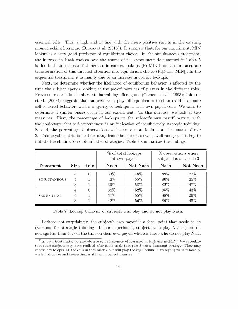
determine if similar biases occur in our experiment. To this purpose, we look at two

measures. First, the percentage of lookups on the subject’s own payoff matrix, with

the conjecture that self-centeredness is an indication of insufficiently strategic thinking.

Second, the percentage of observations with one or more lookups at the matrix of role

3. This payoff matrix is farthest away from the subject’s own payoff and yet it is key to

initiate the elimination of dominated strategies. Table 7 summarizes the findings.

% of total lookups % observations whereat own payoff subject looks at role 3

Treatment Size Role Nash Not Nash Nash Not Nash

4 0 33% 48% 89% 27%simultaneous 4 1 42% 55% 80% 25%

3 1 39% 58% 82% 47%

4 0 38% 52% 85% 43%sequential 4 1 37% 55% 88% 29%

3 1 42% 56% 89% 45%

Table 7: Lookup behavior of subjects who play and do not play Nash.

Perhaps not surprisingly, the subject’s own payoff is a focal point that needs to be

overcome for strategic thinking. In our experiment, subjects who play Nash spend on

average less than 40% of the time on their own payoff whereas those who do not play Nash

10In both treatments, we also observe some instances of increases in Pr[Nash | notMIN]. We speculatethat some subjects may have realized after some trials that role 3 has a dominant strategy. They maychoose not to open all the cells in that matrix but still play the equilibrium. This highlights that lookup,while instructive and interesting, is still an imperfect measure.

14

spend more than 50%. The difference in the likelihood of looking at role 3’s matrix is even

more striking. Supporting the findings in Table 6, subjects who reach the equilibrium

strategy fail to look at the crucial payoff matrix of role 3 only 15% of the time. By

contrast, those who do not play Nash miss that matrix about 64% of the time.

3.4 Transitions of lookups

In section 3.1 we have established that aggregate behavior is different in the simultaneous

and sequential treatments only for role 1 in four-player games. Attentional data can inform

us if differences in the cognitive processes are at the origin of these differences in choices.

It may even be the case that behavior of role 0 in four-player games and role 1 in three-

player games is similar but the cognitive processes are not. To study this question in more

detail, we analyze the sequence of lookups.

Mousetracking provides an enormous amount of data that can be disaggregated in

many ways. Here, we propose the following analysis. For each subject in each game we

determine which role’s payoff matrix a subject opens (independently of the cell within

that matrix), and then record all the transitions between matrices (from a cell in role i’s

payoff matrix to a cell in role j’s payoff matrix, etc.).11 This means that we ignore the

number of clicks in a cell as well as the transitions within a role i’s matrix.

Denoting ij the transition from the payoff matrix of role i to the payoff matrix of role

j, we can group these transitions in three main categories. First, “action” transitions.

These are the transitions from the matrix of role i to the matrix of the role affected by the

action of role i: (32, 21, 10, 03) in four-player games and (32, 21, 13) in three-player games.

They include all backward adjacent transitions as well as the transition from first to last

role, which wraps up the argument.12 These transitions follow the induction argument

which is key to solve the game: “if i choses action ai, then i−1 should choose action ai−1,

etc.” Second, “payoff” transitions. These are the transitions from the matrix of role i to

the matrix of the role whose action will affect the payoff of role i: (01, 12, 23, 30) in four-

player games and (12, 23, 31) in three-player games. They include all forward adjacent

transitions as well as the transition from last to first role. These are natural transitions

to look at, in order to determine potential payoffs associated to the action of a certain

role, but they are misleading in that they do not help solving the game. All transitions

in three-player games are either action or payoff transitions. The remaining transitions in

four-player games are what we call “non-adjacent” transitions: (02, 13, 20, 31).

11For this particular analysis of lookup transitions, it is key that each matrix contains payoffs of one andonly one role.

12For a subject who realizes that role 3 has a dominant strategy, the transition from first to last role isunnecessary. However, we should not presuppose that our subjects have such sophisticated knowledge.

15

Table 8 presents for role 0 in four-player games and for role 1 in three- and four-player

games, the fraction of between-matrices transitions that are of the action, payoff and non-

adjacent type, respectively. We are interested in studying differences in cognitive processes

between simultaneous and sequential treatments by subjects who play the equilibrium

strategy. We therefore consider the two treatments separately and restrict attention to

observations consistent with equilibrium. Finally, we also disaggregate the data into early,

late and all matches together.

simultaneous

action payoff non-adjacent

Size Role early late all early late all early late all

4 0 .56 .58 .57 .42 .41 .41 .02 .01 .021 .55 .57 .57 .41 .38 .39 .05 .05 .05

3 1 .53 .63 .58 .47 .37 .42 – – –

sequential

action payoff non-adjacent

Size Role early late all early late all early late all

4 0 .67 .81 .75 .31 .16 .22 .02 .03 .031 .62 .78 .69 .31 .19 .26 .07 .03 .06

3 1 .72 .82 .76 .28 .18 .24 – – –

Table 8: Percentage of action, payoff and non-adjacent transitions for Nash players

According to Table 8, the pattern of transitions is very different between the sequential

and simultaneous treatments, even though we consider only observations where subjects

play the equilibrium action. At the same time, differences are stable across roles and

group size. As expected, non-adjacent transitions are always rare. More interestingly, the

overall ratio between action and payoff transitions is around 3 in the sequential treatment

(75%-25%) and 1.5 in the simultaneous treatment (60%-40%), whereas random transitions

would predict a ratio of 1. The difference is even more dramatic if we consider only the last

12 matches since the ratio remains constant in the simultaneous treatment and reaches

4.5 in the sequential. The result suggests that imposing a sequential order of play directs

subjects into looking at the matrices in the “right way”, and that this cue provided by

sequentiality becomes more helpful over time. The transitional attentional data is key in

obtaining this result since it holds even when we look exclusively at individuals who choose

16

the equilibrium (and payoff maximizing) strategy. We conjecture that in more complex

games, the cue would translate into larger choice differences (some players who are not

directed to look in the right way, would simply never succeed in finding the equilibrium)

although new data would be necessary to test this hypothesis.

To further investigate the differences in lookup transitions between sequential and

simultaneous treatments, we construct the same table of transitions, except that we con-

dition on the subject having reached the payoff matrix of role 3. More precisely, we remove

all the transitions between matrices that occur before reaching the matrix of role 3 for the

first time. We also remove the observations of individuals who never look at role 3’s ma-

trix.13 The reason for such analysis is the conjecture that a main difficulty in finding the

equilibrium lies in realizing how the behavior of role 3 is the key to unravel the choices of

roles 2, 1 and 0. The outcome is summarized in Table 9.

simultaneous

action payoff non-adjacent

Size Role early late all early late all early late all

4 0 .83 .92 .89 .16 .07 .11 .01 .01 .011 .81 .82 .82 .14 .13 .13 .06 .05 .05

3 1 .79 .89 .85 .21 .11 .15 – – –

sequential

action payoff non-adjacent

Size Role early late all early late all early late all

4 0 .80 .85 .83 .19 .13 .15 .01 .02 .021 .77 .85 .81 .15 .12 .14 .07 .02 .05

3 1 .77 .85 .81 .23 .15 .19 – – –

Table 9: Percentage of action, payoff and non-adjacent transitions for Nash players con-ditional on reaching the payoff matrix of role 3

Once the subject has looked at the payoff matrix of role 3 for the first time, action

transitions become overwhelmingly prevalent (between 81% and 89% of the total). Perhaps

more surprisingly in light of Table 8, the ratio between action and payoff transitions is

now very similar in both treatments. If anything, it is now higher in simultaneous. Also,

the ratio increases in both treatments over the course of the experiment. Overall, Tables 8

13These are only 14% of the observations (recall that we are focusing only on subjects who play Nash).

17

and 9 confirm that the reasoning process is very different in sequential and simultaneous,

even for subjects who play the equilibrium strategy. It also provides an indication of what

these differences are. In simultaneous games, it is harder to realize that the choice of role

3 is key to determine the optimal behavior of roles 2, 1 and 0. As a result, transitions are

more erratic than in sequential games. However, once the payoff matrix of role 3 is hit,

the connection is made and the transition sequence 3-2-1-0 is triggered fast and efficiently

in both treatments.14

3.5 Regression analysis: predicting choice from lookups

The last step of the aggregate analysis consists in using the lookup data to predict choices.

We treat each trial as a separate observation and run Probit regressions to predict whether

the subject plays the equilibrium action (= 1) or not (= 0) in roles 0 and 1. We run six

regressions to study separately the behavior of role 0 in 4H and 4L and role 1 in 4H, 4L,

3H and 3L.

Since we are interested in the predictive power of attentional data, we include variables

related to lookup occurrence and transitions. For occurrence, we introduce a dummy vari-

able that takes value 1 if the subject looked at all the MIN cells, independently of how

many other cells he looked at, and 0 otherwise (min). For transitions, we introduce two

variables: the total number of transitions (total-t) and the percentage of transitions that

are action transitions (action-t). We choose these variables because, according to the re-

sults in sections 3.3 and 3.4, they are good candidates to explain equilibrium behavior. We

can think of other interesting lookup variables, but they will be highly correlated with the

variables in our regression. Finally but crucially, we also add a treatment dummy variable

that takes value 1 in sequential and 0 in simultaneous (seq). The goal is to determine if

differences in behavior across treatments are fully captured by the three lookup variables

described above or if we are still missing some lookup aspect that differentiates equilibrium

choice between treatments. Results are presented in Table 10.

The sign and significance of the parameters are remarkably similar across regressions.

The coefficient for MIN occurrence and action transitions are always highly significant

and indicative of Nash behavior (at the 5% and often at the 0.1% level). This confirms

our previous results that these measures of attention are good predictors of equilibrium

choice. We also find that ‘total transitions’ is either not significant or a negative indicator

of equilibrium choice. It means that, conditional on looking at MIN and having a high

fraction of transitions in the right direction, subjects who spend more time looking at

14Given that we observe learning and that reaching the matrix of role 3 is key, we studied whethersubjects who played in role 3 early in the experiment learned faster to play the Nash equilibrium. Wefound no significant differences.

18

Role 0 Role 0 Role 1 Role 1 Role 1 Role 14H 4L 4H 4L 3H 3L

seq -.135 .103 .213 .460 -.010 -.512∗

(.207) (.211) (.240) (.269) (.180) (.220)

min 1.14∗∗∗ 1.55∗∗∗ 1.83∗∗∗ 1.01∗∗∗ .872∗∗∗ 1.29∗∗∗

(.251) (.256) (.322) (.275) (.234) (.268)

total-t .007 -.006 -.016∗ .004 -.009∗ -.004(.005) (.004) (.006) (.006) (.004) (.004)

action-t 7.10∗∗∗ 5.60∗∗ 8.76∗∗∗ 4.84∗ 5.31∗∗ 4.31∗

(1.84) (1.64) (2.00) (1.92) (1.55) (1.68)

const. -1.19 -.496∗ -.769∗∗ -.110 .008 .229(.243) (.233) (.245) (.278) (.173) (.220)

# obs. 215 216 216 214 288 287Pseudo R2 0.340 0.314 0.430 0.217 0.177 0.307

Standard errors in parentheses. ∗ p < 0.05, ∗∗ p < 0.01, ∗∗∗ p < 0.001

Table 10: Probit regression of Nash behavior as a function of lookups

payoffs perform (weakly) worse. This captures an interesting kind of misguided search (or

wandering) that we will explore in more detail in the next section. Finally but importantly,

the sequence treatment variable is significant in only one regression (role 1 in 3L) and at

the 5% level. It suggests that most differences in choices between the sequential and

simultaneous treatments can be accounted with only two simple attentional measures,

MIN occurrence and action transitions.

3.6 Summary of aggregate analysis

(i) Choice. Nash compliance is reasonably high and increases over time. Level k fits the

aggregate data well though, contrary to the theory, choices for role 1 in four-player games

is different across treatments. (ii) Lookup occurrence. For roles 0 and 1, looking at the

relevant cells is a good predictor of equilibrium behavior: Nash is close to 1 for subjects

who look at MIN and substantially lower for those who do not. (iii) Lookup transition.

The sequence of lookups conditional on equilibrium choice differs across treatments. The

matrix of role 3 is reached faster in sequential. However, once the subject arrives at this

payoff matrix, the unraveling logic of elimination of dominated strategies is performed

equally efficiently in both treatments. (iv) Regression. Probit regressions confirm these

results: MIN occurrence and action transitions have a significant effect in explaining Nash

choices, and there is no treatment effect once we control for these variables.

19

4 Cluster analysis

In this section we use the attentional data to group individuals with the objective of

finding common patterns of lookups. We follow the clustering methodology introduced by

Camerer and Ho (1999) and further developed by Brocas et al. (2013). An advantage of

clustering is that it does not impose any structure of heterogeneity, but rather describes

the heterogeneity found in the data as it is.

As highlighted in section 3, there are many attentional variables that contribute to

explain behavioral choices and these variables are often correlated with each other. In

our experiment, the most promising measures relate to lookup transitions. Indeed, action

transitions are very indicative that the subject is following the logic of strategy elimination.

We will therefore focus on this aspect of attention at the expense of lookup occurrence,

which may be more noisy and variable.15 In any case, which attentional variable (oc-

currence, transitions or a combination of both) explains choices better is ultimately an

empirical question that our data may be able to answer. We will also concentrate on the

choices of roles 0 and 1 for the same reasons as previously.

4.1 Lookup transitions: correct sequence and wandering

One challenge with attentional measures is the large amount of data they provide. For

example, subjects in our experiment open as many as 228 payoff cells in one single trial.

To filter the transition data, we construct a measure analogous to the one we used in

section 3.4. For each observation, we record the string of transitions between the payoff

matrices of the different roles. As before, this ignores the number of clicks as well as the

transitions within a role’s payoff matrix. So, for example, a string ‘132’ for a subject in

role 1 would capture an individual who first opens one or several cells in his own payoff

matrix, then moves to the payoff matrix of role 3 before finally stopping at the matrix of

role 2. For reference, strings in our experiment contain between 0 and 50 digits.

Once these strings are created, we construct two variables for each observation. First,

a dummy variable that takes value 1 if the string contains what we code as the “correct

sequence:” 3210 or 321210 for role 0 and 321 for role 1. The variable takes value 0 otherwise.

The idea is that these sequences are strong indicators that the subject follows the logic

of elimination of dominated strategies from role 3 backwards.16 The second variable is

15In particular, subjects who spend a lot of cognitive effort but are ultimately lost will very likely lookat MIN. By contrast, transitions will look chaotic. Also, subjects who inadvertently miss just one of thecells in the MIN set will be coded as notMIN and yet they may often play the equilibrium.

16For role 0, we allow one forward adjacent transition (12) because a subject may forget some payoffand double check it before restarting the reasoning. Results are almost identical if we allow two forwardadjacent transitions (32121210) or more.

20

the number of matrices open before reaching the correct sequence. This includes the

whole string if the correct sequence is never reached. It provides a measure of how much

the subject looked around before realizing (or not) the correct sequence, which we will

informally refer to as “wandering”. So, for example, strings 01232101 and 13231 for role

1 would be coded as 1 and 0 respectively for the correct sequence variable and 3 and

5 for the wandering variable. Finally, for each individual we compute the percentage of

observations where the correct sequence takes value 1, called %-correct, and the average

number of matrices open before reaching the correct sequence, called pre-correct.17 The

choice of these two variables relies heavily on the analysis in section 3.4, where we reached

two conclusions. First, that lookup transitions widely differ across treatments even among

subjects who play the equilibrium strategy. And second, that heterogeneity is concentrated

on transitions before reaching the matrix of role 3.18

To provide an initial idea of the relationship between correct sequence and equilibrium

behavior, we display in Table 11 the probability that a subject performs the correct se-

quence (Pr[COR]), the probability of Nash conditional on performing the correct sequence

(Pr[Nash |COR]) and the probability of Nash conditional on not performing the correct

sequence (Pr[Nash | notCOR]) for roles 0 and 1. This is the analogue of Table 6 with the

lookup transition variable COR instead of the lookup occurrence variable MIN.

Correct sequence is an excellent predictor of equilibrium behavior. Nash choices are

1.8 to 3.9 more likely given COR than given notCOR. Pr[Nash |COR] slightly increases

over time but the biggest change is the increase in the likelihood of performing the correct

sequence. When we compare the results to those in Table 6, we notice that the increase in

equilibrium choice from notCOR to COR (Pr[Nash |COR]-Pr[Nash |notCOR]) is 3 to 18

percentage points bigger than from notMIN to MIN (Pr[Nash |MIN]-Pr[Nash | notMIN]).

This suggests that correct sequence is a strong indicator, possibly better than MIN lookup,

that the subject understands the unraveling logic of the game.19

17We chose average rather than percentage of pre-correct matrices to distinguish between subjects whodo not reach the correct sequence after opening few boxes v. after opening many boxes.

18We also explored a third variable: the number of matrices open after the correct sequence (which wecalled “post-wandering”). We found little variance across subjects and no systematic patterns for thisvariable so we finally did not include it in the analysis.

19We also conducted an analysis of Nash conditional on performing and not performing the mirror image“forward sequence” (0123 and 012123 for four-player games and 123 for three-player games). We foundthat, after controlling for correct sequence, forward sequence had no explanatory power for Nash behavior.We also noticed that, in accordance to results in section 3.4, subjects in the simultaneous treatment whoperformed the correct sequence typically performed also the forward sequence. By contrast, subjects in thesequential treatment who performed the correct sequence typically did not performed the forward sequence(data omitted fro brevity).

21

simultaneous

Pr[COR] Pr[Nash |COR] Pr[Nash | notCOR]

Size Role early late all early late all early late all

4 0 .40 .69 .54 .86 .97 .93 .22 .29 .241 .44 .69 .57 .94 .95 .94 .32 .52 .39

3 1 .53 .80 .67 .90 .97 .94 .51 .52 .51

sequential

Pr[COR] Pr[Nash |COR] Pr[Nash | notCOR]

Size Role early late all early late all early late all

4 0 .44 .67 .55 .89 .92 .91 .30 .39 .331 .68 .81 .74 .95 .98 .96 .37 .67 .49

3 1 .66 .72 .69 .89 .96 .93 .49 .46 .48

Table 11: Equilibrium choice based on correct sequence (COR)

4.2 Cluster based on lookup transitions

Given the significant differences in lookup transitions between the simultaneous and se-

quential treatments, we decided to perform a separate cluster analysis for subjects in

those treatments. We group the 72 participants of each treatment in clusters based on

the two variables described above, %-correct and pre-correct. There is a wide array of

heuristic clustering methods that are commonly used but they usually require the number

of clusters and the clustering criterion to be set ex-ante rather than endogenously opti-

mized. Mixture models, on the other hand, treat each cluster as a component probability

distribution. Thus, the choice between numbers of clusters and models can be made us-

ing Bayesian statistical methods (Fraley and Raftery, 2002). We implement model-based

clustering analysis with the Mclust package in R (Fraley and Raftery, 2006). We consider

ten different models with a maximum of nine clusters each, and determine the combina-

tion that yields the maximum Bayesian Information Criterion (BIC).20 Technically, this

methodology is the same as Brocas et al. (2013). Conceptually, there are two differences.

20Specifically, hierarchical agglomeration first maximizes the classification likelihood and finds the clas-sification for up to nine clusters for each model. This classification then initializes the Expectation-Maximization algorithm which does maximum likelihood estimation for all possible models and num-ber of clusters combinations. Finally, the BIC is calculated for all combinations with the Expectation-Maximization generated parameters.

22

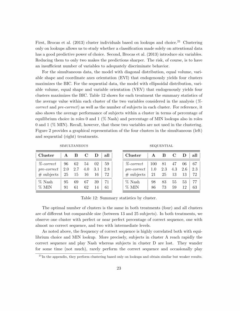
First, Brocas et al. (2013) cluster individuals based on lookups and choice.21 Clustering

only on lookups allows us to study whether a classification made solely on attentional data

has a good predictive power of choice. Second, Brocas et al. (2013) introduce six variables.

Reducing them to only two makes the predictions sharper. The risk, of course, is to have

an insufficient number of variables to adequately discriminate behavior.

For the simultaneous data, the model with diagonal distribution, equal volume, vari-

able shape and coordinate axes orientation (EVI) that endogenously yields four clusters

maximizes the BIC. For the sequential data, the model with ellipsoidal distribution, vari-

able volume, equal shape and variable orientation (VEV) that endogenously yields four

clusters maximizes the BIC. Table 12 shows for each treatment the summary statistics of

the average value within each cluster of the two variables considered in the analysis (%-

correct and pre-correct) as well as the number of subjects in each cluster. For reference, it

also shows the average performance of subjects within a cluster in terms of percentage of

equilibrium choice in roles 0 and 1 (% Nash) and percentage of MIN lookups also in roles

0 and 1 (% MIN). Recall, however, that these two variables are not used in the clustering.

Figure 2 provides a graphical representation of the four clusters in the simultaneous (left)

and sequential (right) treatments.

simultaneous

Cluster A B C D all

%-correct 96 62 54 02 59pre-correct 2.0 2.7 4.0 3.1 2.8# subjects 25 15 16 16 72

% Nash 95 69 67 39 71% MIN 91 61 62 14 61

sequential

Cluster A B C D all

%-correct 100 81 47 06 67pre-correct 1.0 2.3 4.3 2.6 2.3# subjects 21 25 13 13 72

% Nash 98 83 55 53 77% MIN 86 73 59 12 63

Table 12: Summary statistics by cluster.

The optimal number of clusters is the same in both treatments (four) and all clusters

are of different but comparable size (between 13 and 25 subjects). In both treatments, we

observe one cluster with perfect or near perfect percentage of correct sequence, one with

almost no correct sequence, and two with intermediate levels.

As noted above, the frequency of correct sequence is highly correlated both with equi-

librium choice and MIN lookup. More precisely, subjects in cluster A reach rapidly the

correct sequence and play Nash whereas subjects in cluster D are lost. They wander

for some time (not much), rarely perform the correct sequence and occasionally play

21In the appendix, they perform clustering based only on lookups and obtain similar but weaker results.

23

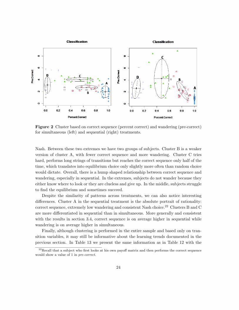
Figure 2 Cluster based on correct sequence (percent correct) and wandering (pre-correct)for simultaneous (left) and sequential (right) treatments.

Nash. Between these two extremes we have two groups of subjects. Cluster B is a weaker

version of cluster A, with fewer correct sequence and more wandering. Cluster C tries

hard, performs long strings of transitions but reaches the correct sequence only half of the

time, which translates into equilibrium choice only slightly more often than random choice

would dictate. Overall, there is a hump shaped relationship between correct sequence and

wandering, especially in sequential. In the extremes, subjects do not wander because they

either know where to look or they are clueless and give up. In the middle, subjects struggle

to find the equilibrium and sometimes succeed.

Despite the similarity of patterns across treatments, we can also notice interesting

differences. Cluster A in the sequential treatment is the absolute portrait of rationality:

correct sequence, extremely low wandering and consistent Nash choice.22 Clusters B and C

are more differentiated in sequential than in simultaneous. More generally and consistent

with the results in section 3.4, correct sequence is on average higher in sequential while

wandering is on average higher in simultaneous.

Finally, although clustering is performed in the entire sample and based only on tran-

sition variables, it may still be informative about the learning trends documented in the

previous section. In Table 13 we present the same information as in Table 12 with the

22Recall that a subject who first looks at his own payoff matrix and then performs the correct sequencewould show a value of 1 in pre-correct.

24

data split between early and late matches.

simultaneous

Cluster A B C D allearly late early late early late early late early late

%-correct 90 100 37 86 32 77 02 03 46 70pre-correct 2.5 1.6 3.0 2.3 4.9 3.0 3.3 3.0 3.3 2.4

% Nash 90 99 49 87 52 83 36 46 61 81% MIN 87 95 41 81 43 81 18 09 52 70

sequential

Cluster A B C D allearly late early late early late early late early late

%-correct 100 100 65 97 39 53 04 10 59 74pre-correct 1.4 0.7 3.4 0.9 4.2 4.4 3.1 2.3 2.9 1.7

% Nash 99 98 71 95 46 65 49 58 70 83% MIN 88 85 66 81 53 68 05 18 58 68

Table 13: Statistics by cluster in early (first 12) and late (last 12) matches.

There is substantial heterogeneity in learning across subjects. The amount of learning–

in terms of more correct sequences, less wandering and more Nash choices– by subjects in

clusters B and C is important. Over time, subjects in cluster B play almost as well as the

highly rational cluster A subjects. This means that, by the end of the experiment, 56%

of subjects in the simultaneous treatment and 64% in the sequential treatment perform

the correct sequence, limit the wandering, and play Nash, providing an excellent template

for rational choice and information processing. The improvement is less pronounced for

subjects in cluster C (especially in the sequential treatment) but still significant. By

contrast, subjects in the other clusters exhibit very limited learning, which is natural

since their level of understanding of the game is either complete from the outset (cluster

A) or extremely limited by the end (cluster D).

4.3 Clusters and level k

In section 3.1 we argued that level k theory provides a reasonably good fit of the aggregate

data. We now study if subjects who belong to a certain cluster exhibit choices consistent

with a specific level of reasoning. This is a stringent test because clustering is performed

25

on attentional variables that are only indirectly related to level k.

In Table 14 we present the probability of Nash choices by role and type of game for

each cluster separately, with darker shades reflecting a substantial drop in Nash choice.

This is the analogue of Table 4 for each subpopulation.

cluster A0 1 2 3

4H .89 .91 .97 1.03H — .95 .96 1.04L .97 .91 1.0 .963L — .98 .92 1.0

cluster A0 1 2 3

4H .92 1.0 .93 1.03H — 1.0 1.0 1.04L .96 1.0 1.0 1.03L — .98 .98 1.0

simultaneous

cluster B0 1 2 3

4H .52 .63 1.0 1.03H — .66 .97 1.04L .50 .85 1.0 1.03L — .97 .97 1.0

sequential

cluster B0 1 2 3

4H .73 .80 .91 1.03H — .85 .93 1.04L .76 .92 1.0 .973L — .89 .98 1.0

cluster C0 1 2 3

4H .60 .54 .89 1.03H — .62 .94 .974L .56 .86 1.0 1.03L — .88 .97 1.0

cluster C0 1 2 3

4H .37 .56 .82 1.03H — .52 .88 1.04L .42 .83 .90 .63L — .56 1.0 1.0

cluster D0 1 2 3

4H .21 .22 .46 .963H — .46 .47 .964L .35 .54 .80 1.03L — .52 .79 .97

cluster D0 1 2 3

4H .33 .50 .59 .813H — .44 .52 .964L .61 .71 .75 1.03L — .61 .79 .94

Table 14: Probability of Nash choice by cluster (darker shade reflects substantial drop inNash rates).

If all subjects in a cluster perfectly fitted a certain level, we would observe Nash choices

with probabilities either 1 or 0 depending on role and type. More realistically, we expect

a significant drop in Nash between the situations where a certain level k predicts Nash

behavior and those where it predicts non-Nash behavior, and that the drop will correspond

to a different combination of role and type of game in different clusters.

The results for the simultaneous treatment are sharp. Cluster A consistently plays

Nash in all roles and types of games, with probabilities ranging from .89 to 1.0. They

correspond to equilibrium (or, equivalently, level 4) players. Clusters B and C are similar

in terms of choice. They play Nash with very high probability when equilibrium requires

to be a level 2 player (.85 and above), and significantly less often when equilibrium requires

to be a level 3 or 4, although these probabilities are still a long way from 0 (.50 to .66).

Combined with Table 12, we notice that the main characteristic that differentiates these

two clusters is not their choice, MIN occurrence or correct sequence; it is mostly the time

26

they spend wandering before realizing (or not) the logic of strategy elimination. These

clusters either mix level 2 and level 4 players or have players starting as level 2 and

become level 4 by the end of the experiment. Given the results in Table 13, we favor

the first explanation for cluster C and the second for cluster B, although we do not have

enough data for a proper test of this conjecture.23 Finally, cluster D is a good prototype

of level 1 players, with high Nash compliance when there is a dominant strategy (role 3)

or when equilibrium requires best response to random behavior (role 2 in type-L games),

and a significant drop when finding the equilibrium requires any sophisticated reasoning.

Level k theory does not fit the data nearly as sharply in the sequential treatment. For

example, cluster C subjects play Nash less often than predicted by level 2 theory in 3L role

1 (.56) and cluster D subjects play Nash more often than predicted by level 1 theory in

4L role 1 (.71). Cluster B does not fit any level: equilibrium choice consistently decreases

with complexity but without a sharp drop at any given role. This is in part due to the

subjects’ ability to learn since, as we highlighted previously, their behavior is very close

to equilibrium (or level 4) in the second-half of the experiment. The link between clusters

and level k theory will be further investigated in the next section.

4.4 Summary of cluster analysis

Two measures of lookup transitions, correct sequence and wandering, naturally divide the

population into four clusters in both treatments: one that reaches the correct sequence

fast, does it systematically, and always plays Nash; one that wanders for a while, rarely

reaches the correct sequence and do not play Nash; and two with intermediate levels of

correct sequence, of which one has significantly more wandering than the other. These

measures correlate well with level k choices in the simultaneous treatment but not in the

sequential treatment. There is learning over time by some subjects. By the end of the

experiment, 60% of the population exhibits rational choice and well-directed attention.

5 Individual analysis

In this section we perform a structural estimation of individual behavior. Following Costa-

Gomes et al. (2001), we assume that subjects have a type that is drawn from a common

prior distribution, and that this type remains constant over the 24 matches.24 The sub-

ject’s behavior is determined by her type, possibly with some error. We also assume that

23For a structural estimation of learning in beauty contest games based on level k reasoning, see Gilland Prowse (2012).

24Given the documented learning, this is unsatisfactory. Unfortunately, we do not have enough obser-vations to perform an individual estimation if we use only the last 12 matches.

27

subjects treat each match as strategically independent. In specifying the possible types, we

use some of the general behavioral principles that have been emphasized in the literature

as being most relevant. We consider the following set of types. Pessimistic [Pes] (subjects

who maximize the minimum payoff over the rival’s decision), Optimistic [Opt ] (subjects

who maximize the maximum payoff over the rival’s decision), Sophisticated [Sop] (sub-

jects who best respond to the aggregate empirical distribution of choices) and Equilibrium

[NE ] (subjects who play Nash). We also include the types corresponding to the steps of

dominance and level k theories: L1, L2, L3, L4, D1, D2, D3 as described in section 2.1.

This set of 11 types is chosen to be large and diverse enough to accommodate a variety

of possible strategies without overly constraining the data analysis, yet small enough to

avoid overfitting.25 Each of our types predicts an action for each role in each game.

5.1 Econometric model

For the econometric analysis we focus exclusively on decisions.26 In order to determine

how distinctive the behavior of each type is, we first compute the matrix of correlations

of choices for the different types. More precisely, for each observation of an individual

and given the role and type of game, we determine whether the action chosen by the

subject is consisted with each of the considered types (coded as 1) or not (coded as 0).

Naturally, actions will typically be consisted with a subset of types. We then sum up the

24 observations of the individual and calculate the partial correlation matrix for all our

types across all individuals. Since D3 and L4 subjects play Nash in all games, they are

indistinguishable from [NE ], so we omit them from the analysis. The results are presented

in Table 15 separately for the simultaneous and sequential treatments.

As we already knew from section 3.2, [Sop] play Nash in almost all games and roles,

hence the high correlation with [NE ]. [Opt ] are also rarely separated from L1 and so

are D2 from L3. Given these correlations, for the econometric analysis we keep 6 types:

τ ∈ T = {Pes, D1, L1, L2, L3,NE}.27

We conduct a maximum likelihood error-rate analysis of subjects’ decisions with the

6 types of players discussed above using the econometric model of Costa-Gomes et al.

25Costa-Gomes and Crawford (2006) also include “pseudo types,” defined as types constructed fromeach of the subjects’ empirical behavior in their experiment (for a total of 88 types). Pseudo types hadlittle explanatory power in their data so we decided not to follow that route.

26Ideally, we would like to classify individuals according to choices and lookups. In a previous version(omitted for brevity) we performed such exercise. However, the results were not robust mainly because wedo not have enough observations to estimate the large number of parameters.

27We realize this biases the results in favor of level k theory since all 4 relevant levels are kept. Weperformed the analysis (i) with D2 instead of L3 and (ii) with neither D2 nor L3 and found similar resultsmostly because, as we will see below, L3 and D2 subjects are rare in the sequential treatment and almostnon-existent in the simultaneous.

28

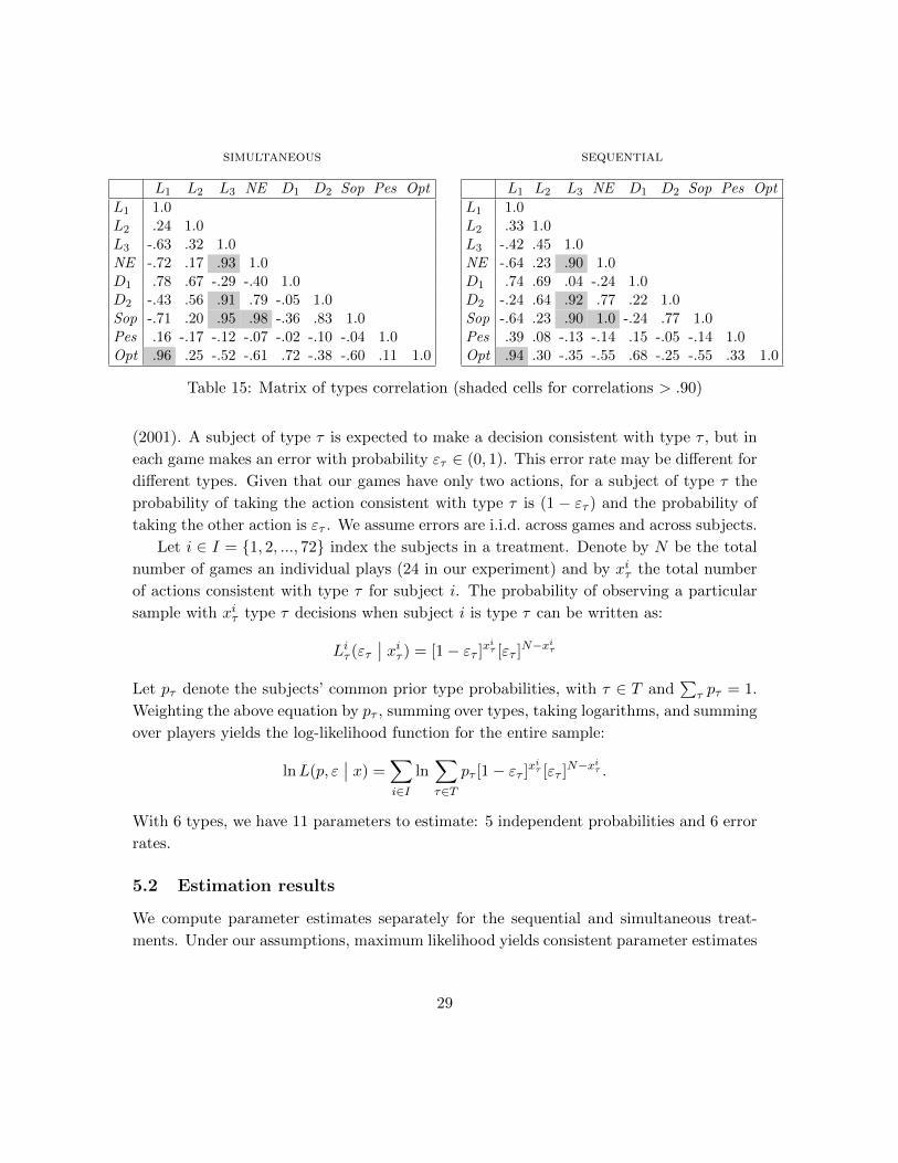
simultaneous

L1 L2 L3 NE D1 D2 Sop Pes Opt

L1 1.0L2 .24 1.0L3 -.63 .32 1.0NE -.72 .17 .93 1.0D1 .78 .67 -.29 -.40 1.0D2 -.43 .56 .91 .79 -.05 1.0Sop -.71 .20 .95 .98 -.36 .83 1.0Pes .16 -.17 -.12 -.07 -.02 -.10 -.04 1.0Opt .96 .25 -.52 -.61 .72 -.38 -.60 .11 1.0

sequential

L1 L2 L3 NE D1 D2 Sop Pes Opt

L1 1.0L2 .33 1.0L3 -.42 .45 1.0NE -.64 .23 .90 1.0D1 .74 .69 .04 -.24 1.0D2 -.24 .64 .92 .77 .22 1.0Sop -.64 .23 .90 1.0 -.24 .77 1.0Pes .39 .08 -.13 -.14 .15 -.05 -.14 1.0Opt .94 .30 -.35 -.55 .68 -.25 -.55 .33 1.0

Table 15: Matrix of types correlation (shaded cells for correlations > .90)

(2001). A subject of type τ is expected to make a decision consistent with type τ , but in

each game makes an error with probability ετ ∈ (0, 1). This error rate may be different for

different types. Given that our games have only two actions, for a subject of type τ the

probability of taking the action consistent with type τ is (1 − ετ ) and the probability of

taking the other action is ετ . We assume errors are i.i.d. across games and across subjects.

Let i ∈ I = {1, 2, ..., 72} index the subjects in a treatment. Denote by N be the total

number of games an individual plays (24 in our experiment) and by xiτ the total number

of actions consistent with type τ for subject i. The probability of observing a particular

sample with xiτ type τ decisions when subject i is type τ can be written as:

Liτ (ετ∣∣ xiτ ) = [1− ετ ]x

iτ [ετ ]N−x

iτ

Let pτ denote the subjects’ common prior type probabilities, with τ ∈ T and∑

τ pτ = 1.

Weighting the above equation by pτ , summing over types, taking logarithms, and summing

over players yields the log-likelihood function for the entire sample:

lnL(p, ε∣∣ x) =

∑i∈I

ln∑τ∈T

pτ [1− ετ ]xiτ [ετ ]N−x

iτ .

With 6 types, we have 11 parameters to estimate: 5 independent probabilities and 6 error

rates.

5.2 Estimation results

We compute parameter estimates separately for the sequential and simultaneous treat-

ments. Under our assumptions, maximum likelihood yields consistent parameter estimates

29

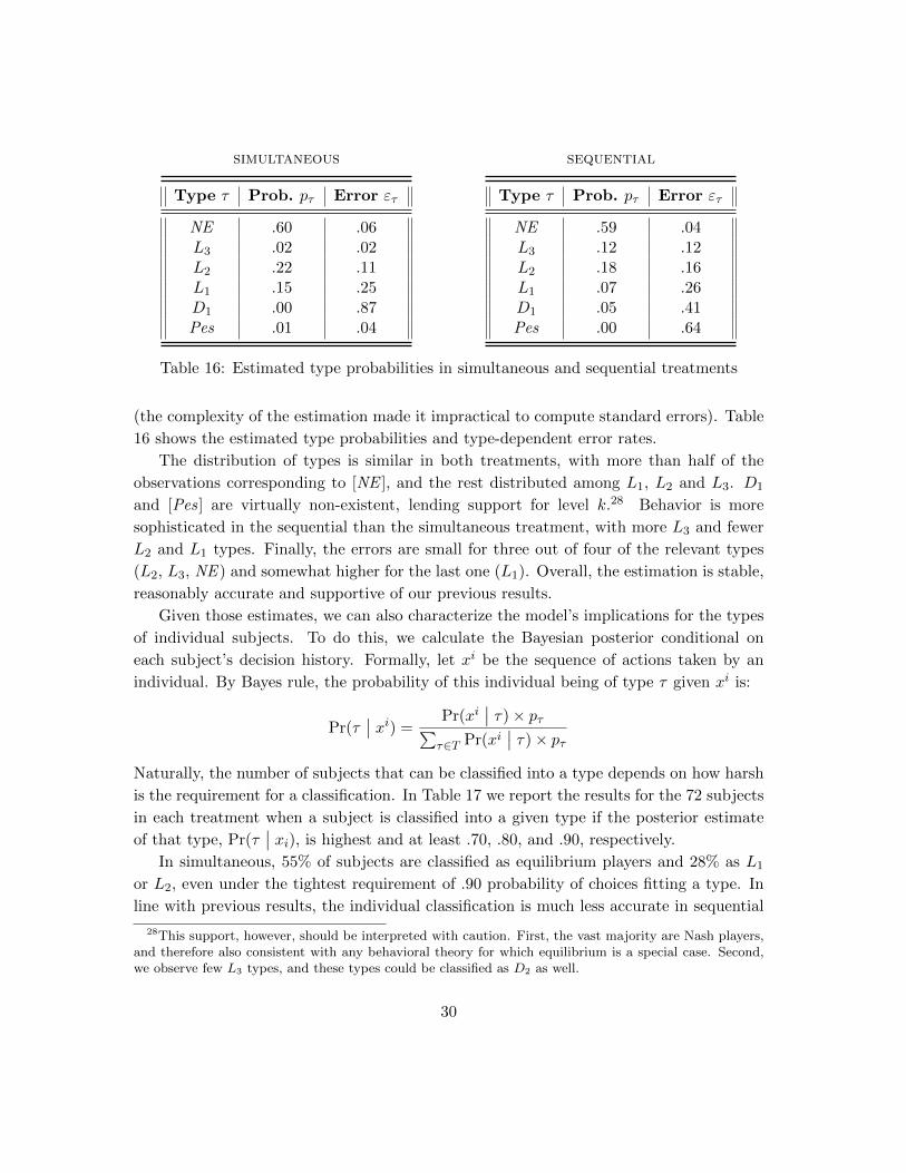
simultaneous

Type τ Prob. pτ Error ετ

NE .60 .06L3 .02 .02L2 .22 .11L1 .15 .25D1 .00 .87Pes .01 .04

sequential

Type τ Prob. pτ Error ετ

NE .59 .04L3 .12 .12L2 .18 .16L1 .07 .26D1 .05 .41Pes .00 .64

Table 16: Estimated type probabilities in simultaneous and sequential treatments

(the complexity of the estimation made it impractical to compute standard errors). Table

16 shows the estimated type probabilities and type-dependent error rates.

The distribution of types is similar in both treatments, with more than half of the

observations corresponding to [NE ], and the rest distributed among L1, L2 and L3. D1

and [Pes] are virtually non-existent, lending support for level k.28 Behavior is more

sophisticated in the sequential than the simultaneous treatment, with more L3 and fewer

L2 and L1 types. Finally, the errors are small for three out of four of the relevant types

(L2, L3, NE ) and somewhat higher for the last one (L1). Overall, the estimation is stable,

reasonably accurate and supportive of our previous results.

Given those estimates, we can also characterize the model’s implications for the types

of individual subjects. To do this, we calculate the Bayesian posterior conditional on

each subject’s decision history. Formally, let xi be the sequence of actions taken by an

individual. By Bayes rule, the probability of this individual being of type τ given xi is:

Pr(τ∣∣ xi) =

Pr(xi∣∣ τ)× pτ∑

τ∈T Pr(xi∣∣ τ)× pτ

Naturally, the number of subjects that can be classified into a type depends on how harsh

is the requirement for a classification. In Table 17 we report the results for the 72 subjects

in each treatment when a subject is classified into a given type if the posterior estimate

of that type, Pr(τ∣∣ xi), is highest and at least .70, .80, and .90, respectively.

In simultaneous, 55% of subjects are classified as equilibrium players and 28% as L1

or L2, even under the tightest requirement of .90 probability of choices fitting a type. In

line with previous results, the individual classification is much less accurate in sequential

28This support, however, should be interpreted with caution. First, the vast majority are Nash players,and therefore also consistent with any behavioral theory for which equilibrium is a special case. Second,we observe few L3 types, and these types could be classified as D2 as well.

30

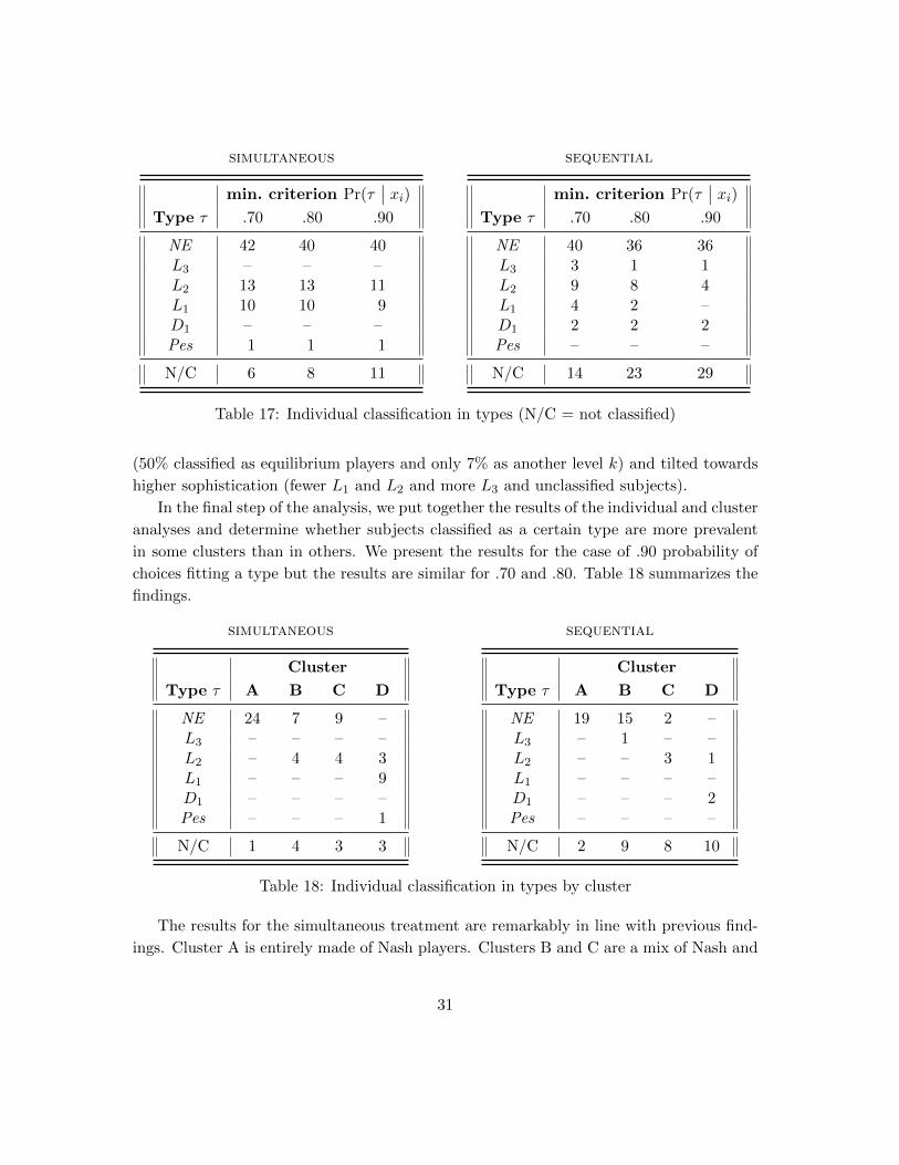
simultaneous

min. criterion Pr(τ∣∣ xi)

Type τ .70 .80 .90

NE 42 40 40L3 – – –L2 13 13 11L1 10 10 9D1 – – –Pes 1 1 1

N/C 6 8 11

sequential

min. criterion Pr(τ∣∣ xi)

Type τ .70 .80 .90

NE 40 36 36L3 3 1 1L2 9 8 4L1 4 2 –D1 2 2 2Pes – – –

N/C 14 23 29

Table 17: Individual classification in types (N/C = not classified)

(50% classified as equilibrium players and only 7% as another level k) and tilted towards

higher sophistication (fewer L1 and L2 and more L3 and unclassified subjects).

In the final step of the analysis, we put together the results of the individual and cluster

analyses and determine whether subjects classified as a certain type are more prevalent

in some clusters than in others. We present the results for the case of .90 probability of

choices fitting a type but the results are similar for .70 and .80. Table 18 summarizes the

findings.

simultaneous

Cluster

Type τ A B C D

NE 24 7 9 –L3 – – – –L2 – 4 4 3L1 – – – 9D1 – – – –Pes – – – 1

N/C 1 4 3 3

sequential

Cluster

Type τ A B C D

NE 19 15 2 –L3 – 1 – –L2 – – 3 1L1 – – – –D1 – – – 2Pes – – – –

N/C 2 9 8 10

Table 18: Individual classification in types by cluster

The results for the simultaneous treatment are remarkably in line with previous find-

ings. Cluster A is entirely made of Nash players. Clusters B and C are a mix of Nash and

31

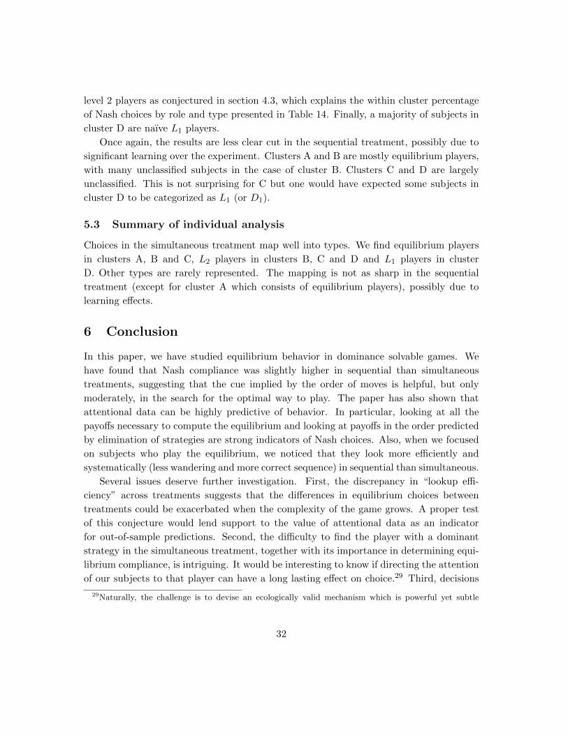
level 2 players as conjectured in section 4.3, which explains the within cluster percentage

of Nash choices by role and type presented in Table 14. Finally, a majority of subjects in

cluster D are naıve L1 players.

Once again, the results are less clear cut in the sequential treatment, possibly due to

significant learning over the experiment. Clusters A and B are mostly equilibrium players,

with many unclassified subjects in the case of cluster B. Clusters C and D are largely

unclassified. This is not surprising for C but one would have expected some subjects in

cluster D to be categorized as L1 (or D1).

5.3 Summary of individual analysis

Choices in the simultaneous treatment map well into types. We find equilibrium players

in clusters A, B and C, L2 players in clusters B, C and D and L1 players in cluster

D. Other types are rarely represented. The mapping is not as sharp in the sequential

treatment (except for cluster A which consists of equilibrium players), possibly due to

learning effects.

6 Conclusion

In this paper, we have studied equilibrium behavior in dominance solvable games. We

have found that Nash compliance was slightly higher in sequential than simultaneous

treatments, suggesting that the cue implied by the order of moves is helpful, but only

moderately, in the search for the optimal way to play. The paper has also shown that

attentional data can be highly predictive of behavior. In particular, looking at all the

payoffs necessary to compute the equilibrium and looking at payoffs in the order predicted

by elimination of strategies are strong indicators of Nash choices. Also, when we focused

on subjects who play the equilibrium, we noticed that they look more efficiently and

systematically (less wandering and more correct sequence) in sequential than simultaneous.

Several issues deserve further investigation. First, the discrepancy in “lookup effi-

ciency” across treatments suggests that the differences in equilibrium choices between

treatments could be exacerbated when the complexity of the game grows. A proper test

of this conjecture would lend support to the value of attentional data as an indicator

for out-of-sample predictions. Second, the difficulty to find the player with a dominant

strategy in the simultaneous treatment, together with its importance in determining equi-

librium compliance, is intriguing. It would be interesting to know if directing the attention

of our subjects to that player can have a long lasting effect on choice.29 Third, decisions

29Naturally, the challenge is to devise an ecologically valid mechanism which is powerful yet subtle

32

could be affected by the presentation of the game. In our design, it is always the right-

most player who has the dominant strategy. We believe that subjects would be cued if

the last mover always had the dominant strategy (which we have to for comparison with

simultaneous) but her position in the screen (rightmost, center, leftmost) changed from

game to game. However, this is an empirical question. Overall, we believe that choice and

non-choice data are strongly complementary measures and that experimental research in

that direction will improve our understanding of (the limits to) human cognition.

enough to avoid demand effects from the experimenter.

33

References

1. Armel, C., Beaumel, A. and A. Rangel (2008) “Biasing simple choices by manipu-lating relative visual attention”, Judgment and Decision Making, 3(5): 396-403.

2. Armel, C. and A. Rangel (2008) “The impact of computation time and experienceon decision values”, American Economic Review, 98: 163-168.

3. Brocas, I., Carrillo, J.D., Wang, S. and C. Camerer (2013) “Imperfect choice or im-perfect attention? Understanding strategic thinking in private information games”,forthcoming in Review of Economic Studies.

4. Camerer, C. and T. Ho (1999) “Experience-weighted attraction learning in normalform games”, Econometrica, 67: 827-874.

5. Camerer, C. and E. Johnson (2004) “Thinking About Attention in Games: Backwardand Forward Induction” in I. Brocas and J.D. Carrillo (eds.) The Psychology ofEconomic Decisions, Vol 2. Reasons and Choices, Oxford University Press: Oxford,UK, 111-130.

6. Camerer, C., Johnson, E., Rymon, T. and S. Sen (1993) “Cognition and framing insequential bargaining for gains and losses”, in K. Binmore, A. Kirman and P. Tani(eds.) Frontiers of Game Theory, Cambridge, MIT Press: 27-47.

7. Carrillo, J.D. and T. Palfrey (2009) “The Compromise Game: Two-Sided AdverseSelection in the Laboratory”, American Economic Journal: Microeconomics, 151-181.

8. Charness, G. and M. Rabin (2002) “Understanding social preferences with simpletests”, Quarterly Journal of Economics, 117: 817-869.

9. Cooper, D and J. Van Huyck (2003) “Evidence on the Equivalence of the Strategicand Extensive Form Representation of Games”, Journal of Economic Theory, 110:290-308.

10. Costa-Gomes, M. and V. Crawford (2006) “Cognition and Behavior in Two-Personguessing Games: An Experimental Study”, American Economic Review, 96(5):1737-1768.

11. Costa-Gomes, M., Crawford, V. and B. Broseta (2001) “Cognition and behavior innormal-form games: An experimental study”, Econometrica, 69(5): 1193-1235.

12. Crawford, V. (2008), “Look-Ups As The Windows Of The Strategic Soul: StudyingCognition Via Information Search In Game Experiments”, In A. Caplin and A.Schotter (eds.), Perspectives on the Future of Economics: Positive and NormativeFoundations, Oxford University Press, Oxford: UK.

34

13. Crawford, V., Costa-Gomes, M. and N. Iriberri (2013) “Structural Models of Nonequi-librium Strategic Thinking: Theory, Evidence, and Applications”, Journal of Eco-nomic Literature, 5-62.

14. Devetag, G., Di Guida, S. and L. Polonio (2013) “An eye-tracking study of feature-based choice in one-shot games”, LEM Working paper, 2013/05.

15. Fehr, E. and K. Schmidt (1999) “A theory of fairness, competition, and cooperation”,Quarterly Journal of Economics, 114: 817-868.

16. Fraley, C. and A. E. Raftery (2002) “Model-based clustering, discriminant analysis,and density estimation”, Journal of the American Statistical Association, 97: 611-631.

17. Fraley, C. and A. E. Raftery (2006) “MCLUST version 3 for R: normal mixture mod-eling and model-based clustering”, Technical report 504, University of Washington.

18. Gill, D. and V. Prowse (2012) “Cognitive ability and learning to play equilibrium:A level-k analysis”, MPRA Paper 38317, University Library of Munich, Germany.

19. Glazer J. and A. Rubinstein (1996) “An extensive game as a guide for solving anormal game”, Journal of Economic Theory, 70: 32-42.

20. Johnson, E.J., Camerer, C.F., Sen, S. and T. Rymon (2002) “Detecting Failuresof Backward Induction: Monitoring Information Search in Sequential Bargaining”,Journal of Economic Theory, 104: 16-47.

21. Katok, E., Sefton, M. and A. Yavas (2002) “Implementation by Iterative Dominanceand Backward Induction: An Experimental Comparison”, Journal of Economic The-ory, 104: 89-103.

22. Kneeland, T. (2013) “Testing behavioral game theory: higher-order rationality andconsistent beliefs” mimeo, University College London.

23. Knoepfle, D., Wang, J., and C. Camerer (2009) “Studying learning in games usingeyetracking”, Journal of the European Economic Association, 7: 388-398.

24. Kohlberg, E. and J.F. Mertens (1986) “On the Strategic Stability of Equilibria”,Econometrica, 54(5): 1003-1037.

25. Luce, R.D. (1992) “Rational versus plausible accounting equivalences in preferencejudgments”, in W. Edwards (ed.) Utility theories: Measurements and applications.Kluwer Academic Press, Boston: 187-206.

26. McCabe, K.A., Smith, V.L. and M. LePore (2000) “Intentionality detection and‘mindreading’: Why does game form matter?” Proceedings of the National Academyof Sciences, 97(8): 4404-09.

35

27. Rapoport, A. (1997) “Order of play in strategically equivalent games in extensiveform”, International Journal of Game Theory, 26: 113-136.

28. Reutskaja, E., Nagel, R., Camerer, C.F. and A. Rangel (2011) “Search Dynam-ics in Consumer Choice under Time Pressure: An Eye-Tracking Study”, AmericanEconomic Review, 101: 900-926.

29. Schotter, A., Weigelt, K. and C. Wilson (1994) “A laboratory investigation of multi-person rationality and presentation effects”, Games and Economic Behavior, 6: 164-212.

30. Wang, J.T., Spezio, M. and C. Camerer (2010) “Pinocchio’s Pupil: Using Eye-tracking and Pupil Dilation to Understand Truth Telling and Deception in Sender-Receiver Games”, American Economic Review, 100(3): 984-1007.

36

Supplementary Appendix

Appendix A. Payoff variants used in the experiment

payoffs

Variant Matches Size Type Role 0 Role 1 Role 2 Role 3

1 1, 7 4 H 28 12 4 25 10 20 10 1410 24 20 5 25 10 20 26

2 10, 19 4 H 15 25 38 18 14 36 34 2630 14 18 32 30 10 20 12

3 20, 23 4 H 15 30 16 28 15 35 18 2424 16 30 20 32 10 10 12

4 2, 14 4 L 15 25 8 18 14 6 10 1426 10 20 10 6 18 18 24

5 5, 11 4 L 10 22 25 15 28 14 22 3218 10 15 30 12 24 14 20

6 15, 21 4 L 32 16 16 34 18 6 10 822 30 30 22 8 22 18 14

7 3, 9 3 H 4 25 10 20 10 1420 5 25 10 24 30

8 6, 13 3 H 6 22 12 28 18 1228 8 22 10 10 6

9 12, 17 3 H 4 20 8 22 10 815 5 25 10 26 22

10 4, 24 3 L 22 8 10 28 12 1010 25 22 12 24 20

11 8, 18 3 L 12 22 10 16 18 1428 10 18 10 10 8

12 16, 22 3 L 4 25 10 25 12 2020 5 20 12 22 32

Table 19: Payoff-Variants

37

Appendix B. Sample of Instructions (simultaneous treatment)

Thanks for participating in this experiment on group decision-making. During the experiment we wouldlike to have your undistracted attention. Do not open other applications on your computer, chat withother students, use headphones, read, etc. Make sure to turn your phone to silent mode and not use itduring the experiment.

You will be paid for your participation in cash at the end of the experiment. Different participantsmay earn different amounts. What you earn depends partly on your decisions, partly on the decisions ofothers, and partly on chance. The entire experiment will take place through computer terminals, and allinteraction between participants will take place through the computers. Do not talk or in any way try tocommunicate with other participants during the experiment.

We will start with a brief instruction period. During the instruction period, you will be given acomplete description of the experiment and will be shown how to use the computers. It is very importantthat you listen carefully and fully understand the instructions since your decisions will affect your earnings.You will be asked some review questions after the instructions, which have to be answered correctly beforewe can begin the experiment. If you have any questions during the instruction period, raise your handand your question will be answered so everyone can hear. If any difficulties arise after the experiment hasbegun, raise your hand, and an experimenter will come and assist you.

At the end of the session, you will be paid the sum of what you have earned in all matches, plus theshow-up fee of $5. Your earnings during the experiment are denominated in tokens. Depending on yourdecisions, you can earn more or less tokens. At the end of the experiment, we will count the number oftokens you have and you will be paid $1.00 for every 30 tokens. Everyone will be paid in private and youare under no obligation to tell others how much you earned.

The experiment consists of 24 matches. In each match, you will be grouped with either two or threeother participants, which means there will be either 3 or 4 participants in a group. Group size will bedifferent for each match. Since there are 12 participants in today’s session, in a match there will be either3 groups of 4 participants or 4 groups of 3 participants. You are not told the identity of the participantsyou are grouped with. Your payoff depends only on your decisions, the decisions of the participants youare grouped with and on chance. What happens in the other groups has no effect on your payoff and viceversa. Your decisions are not revealed to participants in the other groups.

We will present the game using screenshots. Your instruction package includes two separate pages,which are screenshots of computer screens. Look at the first page. I will now describe the screenshot in“Display 1”. Do you have the Display 1 in front of you? Raise your hand high if you do. If you don’t raiseyour hand we will come around and guide your attention to the separate Display 1 page.

In this match each participant is grouped with two other participants. At the beginning of the match,the computer randomly assigns a role to each of the three members in your group as RED or GREEN orBLUE. In each match, each role is asked to make a choice from two possible actions, XR or YR for thesubject in the RED role, XG or YG for the subject in the GREEN role and XB or YB for the subject inthe BLUE role. You will choose an action without knowing which actions the other players in your grouphave chosen.

You will see a screen like the one in Display 1. In this example, you have the GREEN role. The screensays ‘GREEN, please choose an action’. Your action can be either XG or YG.

The payoffs you may obtain are the numbers inside the boxes in the left table. In this example, yourpayoff depends on your action (the rows, XG or YG) and on the action of RED (the columns, XR or YR).For example, if you choose YG and RED chooses XR, then you will earn 80 tokens. If RED chooses YRinstead, then you will earn 132 tokens.

If you are Role RED, you will see a screen similar to Display 1 but it will read, ’RED, please choosean action’. RED must respond by clicking on the XR or YR button. The payoffs RED may obtain are thenumbers inside the middle table. In this example, the payoffs RED may obtain depend on his action andthe action of BLUE. For example, if RED chooses YR and BLUE chooses XB , RED will earn 96 tokens.

38

Finally, the payoffs BLUE may obtain are the numbers inside the right table. Payoffs that BLUE mayobtain depend on his action and the action of GREEN.

Once every member in the group has made a choice, the computer screen will display the actions forall members of your group and your payoff for the match. The payoff is added to your total. This will endthe current match.

When a match is finished, we proceed to the next match. For the next match, the computer randomlyreassigns all participants to a new group and to a new role. The new assignments do not depend in anyway on the past decisions of any participant including you, and are done completely randomly by thecomputer. The assignments are independent across groups, across participants and across matches. Thissecond match then follows the same rules as the first match with two exceptions. First, the payoffs insidethe tables are now different. Second, in the new match you may be grouped with 3 (rather than 2) otherparticipants. If you are grouped with three other participants the roles are “RED”, “GREEN”, “BLUE”and “ORANGE”.

The same procedure continues for 24 matches, after which the experiment ends.A history screen at the bottom will show a rolling history of your role in that match, the actions of

all subjects in your group and your payoff.Now turn to the Display 2. Do you have the Display 2 page in front of you? Raise your hand high if

you do. If you don’t raise your hand we will come around and guide you.This is a similar game but the payoffs are now hidden in boxes. This is the type of screen you will

observe during the experiment. In order to find out what your possible payoffs are, or what the other roles’payoffs are, you must move your mouse into the box that shows the payoff from a particular pair of actionsin the table, and click-and-hold one of the mouse buttons. If you do not hold down the mouse button thepayoff will disappear. When you move the mouse away from the box, the payoff will also disappear. Ifyou move your mouse back into a box, click-and-hold, the exact same payoff will appear again. Clickingdoes not affect your earnings and you can look at as many of the possible payoffs as you care to, or as few,for as long or as briefly as you like. If you have trouble figuring out how to use the mouse to temporarilyreveal the hidden payoffs during the experiment, raise your hand right away and we will come around andhelp you.

Are there any questions? If there are any problems or questions from this point on, raise your handand an experimenter will come and assist you.

39

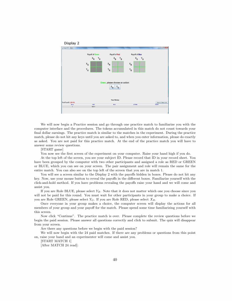
We will now begin a Practice session and go through one practice match to familiarize you with thecomputer interface and the procedures. The tokens accumulated in this match do not count towards yourfinal dollar earnings. The practice match is similar to the matches in the experiment. During the practicematch, please do not hit any keys until you are asked to, and when you enter information, please do exactlyas asked. You are not paid for this practice match. At the end of the practice match you will have toanswer some review questions.

[START game]You now see the first screen of the experiment on your computer. Raise your hand high if you do.At the top left of the screen, you see your subject ID. Please record that ID in your record sheet. You

have been grouped by the computer with two other participants and assigned a role as RED or GREENor BLUE, which you can see on your screen. The pair assignment and role will remain the same for theentire match. You can also see on the top left of the screen that you are in match 1.

You will see a screen similar to the Display 2 with the payoffs hidden in boxes. Please do not hit anykey. Now, use your mouse button to reveal the payoffs in the different boxes. Familiarize yourself with theclick-and-hold method. If you have problems revealing the payoffs raise your hand and we will come andassist you.

If you are Role BLUE, please select YB . Note that it does not matter which one you choose since youwill not be paid for this round. You must wait for other participants in your group to make a choice. Ifyou are Role GREEN, please select YG. If you are Role RED, please select XR.

Once everyone in your group makes a choice, the computer screen will display the actions for allmembers of your group and your payoff for the match. Please spend some time familiarizing yourself withthis screen.

Now click “Continue”. The practice match is over. Please complete the review questions before webegin the paid session. Please answer all questions correctly and click to submit. The quiz will disappearfrom your screen.

Are there any questions before we begin with the paid session?We will now begin with the 24 paid matches. If there are any problems or questions from this point

on, raise your hand and an experimenter will come and assist you.[START MATCH 1][After MATCH 24 read]:

40

This was the last match of the experiment. Your payoff is displayed on your screen. Your final payoffin the experiment is equal to your stock of tokens in the end converted into dollars plus the show-up feeof $5. Please record this payoff in your record sheet and remember to CLICK OK after you are done.

We will pay each of you in private in the next room in the order of your Subject ID number. Rememberyou are under no obligation to reveal your earnings to the other participants. Please put the mouse on theside of the computer and do not use either the mouse or the keyboard. Please remain seated and keep thedividers pulled out until we call you to be paid. Do not converse with the other participants or use yourcell phone. Thank you for your cooperation.

QUIZ

1. In this experiment, your payoffs are presented in boxes. Please choose the correct option:i) Payoffs for all cells are always visible.ii) Payoffs for all cells are hidden. They can be viewed by moving your mouse over the cell and

clicking-and-holding one of the mouse buttons. There is no cost of opening a cell.iii) Payoffs of some cells are hidden and payoffs of other cells are visible.iv) Payoffs for all cells are hidden. They can be viewed by moving your mouse over the cell and

clicking-and-holding one of the mouse buttons. However, tokens are subtracted from your payoff when youview a cell.

2. Look at Display 1. Suppose you are role GREEN. What will be your payoff if you choose XG andRED chooses YR?

i) 72ii) 66iii) It depends on what BLUE chooses

3. What will be the payoff of RED?i) It depends of what BLUE choosesii) 96iii) 112

4. What will be the payoff of BLUE?i) 66ii) 40 if BLUE chooses XB and 66 if BLUE chooses YBiii) 144 if BLUE chooses XB and 94 if BLUE chooses YB

5. Look at Display 1. If actions chosen by all members of the group are XG, YR, YB what will be theearnings of the three roles?

i) GREEN: 72 tokens, RED: 96 tokens, BLUE: 94 tokens.ii) GREEN: 72 tokens, RED: 112 tokens, BLUE: 66 tokens.iii) GREEN: 66 tokens, RED: 112 tokens, BLUE: 66 tokens.

6. Look at Display 2. What is your role and which game table hides your own payoffsi) My role is GREEN and my payoffs are hidden in the middle tableii) My role is BLUE and my payoffs are hidden in the right tableiii) My role is GREEN and my payoffs are hidden in the left tableiv) I cannot know what my role is yet.

41

Appendix C. Determination of MIN set

The MIN set depends on the role, treatment and the actions consistent with Nash. In

sequential, it also depends on the action of the first player (role 0 in 4-player games and

role 1 in 3-player games). We explain MIN with the help of Table 20. The values in this

table are not the payoffs from the game but, instead, the codes of the cells used here to

support the explanation of MIN.

Role 0X1 Y1

X0 1 2Y0 3 4

Role 1X2 Y2

X1 5 6Y1 7 8

Role 2X3 Y3

X2 9 10Y2 11 12

Role 3X0 Y0

X3 13 14Y3 15 16

Table 20: Support table to find MIN (values are not payoffs in the game but instead thecell codes given to facilitate the explanation of MIN)

MIN for simultaneous. Take the convention that the Nash equilibrium is (X0, X1, X2, X3).

MIN for role 3 are cells 13, 14, 15 and 16, since opening this set enables role 3 to figure

out her dominant strategy. MIN for role 2 are cells 13, 14, 15, 16, 9 and 11: opening 13,

14, 15 and 16 enables role 2 to know that X3 is a dominant strategy for role 3 and then

role 2 only needs to open cells 9 and 11, the cells in her payoff matrix corresponding to

X3. Using the same logic we get that MIN for role 1 are cells 13, 14, 15, 16, 9, 11, 5 and

7 and MIN for role 0 are cells 13, 14, 15, 16, 9, 11, 5, 7, 1 and 3.

MIN for sequential. MIN for the first player (role 0 in 4-player games and role 1 in

3-player games) is defined exactly as in the simultaneous treatment. MIN for the other

roles depends on the action taken by the first player. Let us assume that role 0 chooses

X0 in 4-player games (or role 1 chooses X1 in 3-player games). MIN for role 3 are only

cells 13 and 15: role 3 observes the action of role 0 (role 1 in 3-player games) so, in order

to calculate her Nash strategy, she only needs to compare cells 13 and 15 in her payoff

matrix. With an analogous reasoning we get that MIN for role 2 are cells 13, 15, 9 and

11 and MIN for role 1 in 4-player games are cells 13, 15, 9, 11, 5 and 7. Naturally, when

we code MIN in each of our games we need to track which action corresponds to the Nash

equilibrium (Xi or Yi) and which action has been taken by the first player.

42