the particle swarm-explosion, stability, and convergence ... · the particle swarm—explosion,...

58 IEEE TRANSACTIONS ON EVOLUTIONARY COMPUTATION, VOL. 6, NO. 1, FEBRUARY 2002

The Particle Swarm—Explosion, Stability, andConvergence in a Multidimensional Complex Space

Maurice Clerc and James Kennedy

Abstract—The particle swarm is an algorithm for finding op-timal regions of complex search spaces through the interaction ofindividuals in a population of particles. Even though the algorithm,which is based on a metaphor of social interaction, has been shownto perform well, researchers have not adequately explained howit works. Further, traditional versions of the algorithm have hadsome undesirable dynamical properties, notably the particles’ ve-locities needed to be limited in order to control their trajectories.The present paper analyzes a particle’s trajectory as it moves indiscrete time (the algebraic view), then progresses to the view ofit in continuous time (the analytical view). A five-dimensional de-piction is developed, which describes the system completely. Theseanalyses lead to a generalized model of the algorithm, containinga set of coefficients to control the system’s convergence tendencies.Some results of the particle swarm optimizer, implementing modi-fications derived from the analysis, suggest methods for altering theoriginal algorithm in ways that eliminate problems and increasethe ability of the particle swarm to find optima of some well-studiedtest functions.

Index Terms—Convergence, evolutionary computation, opti-mization, particle swarm, stability.

I. INTRODUCTION

PARTICLE swarm adaptation has been shown to suc-cessfully optimize a wide range of continuous functions

[1]–[5]. The algorithm, which is based on a metaphor of socialinteraction, searches a space by adjusting the trajectories ofindividual vectors, called “particles” as they are conceptualizedas moving points in multidimensional space. The individualparticles are drawn stochastically toward the positions oftheir own previous best performance and the best previousperformance of their neighbors.

While empirical evidence has accumulated that the algorithm“works,” e.g., it is a useful tool for optimization, there has thusfar been little insight intohow it works. The present analysisbegins with a highly simplified deterministic version of the par-ticle swarm in order to provide an understanding about how itsearches the problem space [4], then continues on to analyzethe full stochastic system. A generalized model is proposed, in-cluding methods for controlling the convergence properties ofthe particle system. Finally, some empirical results are given,showing the performance of various implementations of the al-gorithm on a suite of test functions.

Manuscript received January 24, 2000; revised October 30, 2000 and April30, 2001.

M. Clerc is with the France Télécom, 74988 Annecy, France (e-mail: [email protected]).

J. Kennedy is with the Bureau of Labor Statistics, Washington, DC 20212USA (e-mail: [email protected]).

Publisher Item Identifier S 1089-778X(02)02209-9.

A. The Particle Swarm

A population of particles is initialized with random positionsand velocities and a function is evaluated, using the par-

ticle’s positional coordinates as input values. Positions and ve-locities are adjusted and the function evaluated with the newcoordinates at each time step. When a particle discovers a pat-tern that is better than any it has found previously, it stores thecoordinates in a vector . The difference between (the bestpoint found by so far) and the individual’s current positionis stochastically added to the current velocity, causing the tra-jectory to oscillate around that point. Further, each particle isdefined within the context of a topological neighborhood com-prising itself and some other particles in the population. Thestochastically weighted difference between the neighborhood’sbest position and the individual’s current position is alsoadded to its velocity, adjusting it for the next time step. Theseadjustments to the particle’s movement through the space causeit to search around the two best positions.

The algorithm in pseudocode follows.

Intialize population

Do

For i = 1 to Population Size

if f(~x ) < f(~p ) then ~p = ~x

~p = min(~p )

For d = 1 to Dimension

v = v + ' (p � x ) + ' (p � x )

v = sign (v ) �min(abs (v ); v )

x = x + v

Next d

Next i

Until termination criterion is met

The variables and are random positive numbers, drawnfrom a uniform distribution and defined by an upper limit ,which is a parameter of the system. In this version, the term vari-able is limited to the range for reasons that will beexplained below. The values of the elements inare deter-mined by comparing the best performances of all the membersof ’s topological neighborhood, defined by indexes of someother population members and assigning the best performer’sindex to the variable . Thus, represents the best positionfound by any member of the neighborhood.

The random weighting of the control parameters in the al-gorithm results in a kind of explosion or a “drunkard’s walk”as particles’ velocities and positional coordinates careen towardinfinity. The explosion has traditionally been contained through

1089–778X/02$17.00 © 2002 IEEE

Authorized licensed use limited to: Universitatsbibliothek der TU Wien. Downloaded on May 04,2010 at 06:41:45 UTC from IEEE Xplore. Restrictions apply.

CLERC AND KENNEDY: THE PARTICLE SWARM—EXPLOSION, STABILITY, AND CONVERGENCE 59

implementation of a parameter, which limits step size orvelocity. The current paper, however, demonstrates that the im-plementation of properly defined constriction coefficients canprevent explosion; further, these coefficients can induce parti-cles to converge on local optima.

An important source of the swarm’s search capability is theinteractions among particles as they react to one another’s find-ings. Analysis of interparticle effects is beyond the scope of thispaper, which focuses on the trajectories of single particles.

B. Simplification of the System

We begin the analysis by stripping the algorithm down to amost simple form; we will add things back in later. The particleswarm formula adjusts the velocityby adding two terms to it.The two terms are of the same form, i.e., , where isthe best position found so far, by the individual particle in thefirst term, or by any neighbor in the second term. The formulacan be shortened by redefining as follows:

Thus, we can simplify our initial investigation by looking atthe behavior of a particle whose velocity is adjusted by only oneterm

where . This is algebraically identical to the stan-dard two-term form.

When the particle swarm operates on an optimizationproblem, the value of is constantly updated, as the systemevolves toward an optimum. In order to further simplify thesystem and make it understandable, we setto a constantvalue in the following analysis. The system will also bemore understandable if we makea constant as well; wherenormally it is defined as a random number between zero and aconstant upper limit, we will remove the stochastic componentinitially and reintroduce it in later sections. The effect ofonthe system is very important and much of the present paper isinvolved in analyzing its effect on the trajectory of a particle.

The system can be simplified even further by considering aone-dimensional (1-D) problem space and again further by re-ducing the population to one particle. Thus, we will begin bylooking at a stripped-down particle by itself, e.g., a populationof one 1-D deterministic particle, with a constant.

Thus, we begin by considering the reduced system

(1.1)

where and are constants. No vector notation is necessaryand there is no randomness.

In [4], Kennedy found that the simplified particle’s trajectoryis dependent on the value of the control parameterand recog-nized that randomness was responsible for the explosion of thesystem, although the mechanism that caused the explosion wasnot understood. Ozcan and Mohan [6], [7] further analyzed thesystem and concluded that the particle as seen in discrete time“surfs” on an underlying continuous foundation of sine waves.

The present paper analyzes the particle swarm as it moves indiscrete time (the algebraic view), then progresses to the view ofit in continuous time (the analytical view). A five-dimensional(5-D) depiction is developed, which completely describes thesystem. These analyses lead to a generalized model of the al-gorithm, containing a set of coefficients to control the system’sconvergence tendencies. When randomness is reintroduced tothe full model with constriction coefficients, the deleterious ef-fects of randomness are seen to be controlled. Some results ofthe particle swarm optimizer, using modifications derived fromthe analysis, are presented; these results suggest methods for al-tering the original algorithm in ways that eliminate some prob-lems and increase the optimization power of the particle swarm.

II. A LGEBRAIC POINT OF VIEW

The basic simplified dynamic system is defined by

(2.1)

where .Let

be the current point in and

the matrix of the system. In this case, we haveand, more generally, . Thus, the system is definedcompletely by .

The eigenvalues of are

(2.2)

We can immediately see that the value is special.Below, we will see what this implies.

For , we can define a matrix so that

(2.3)

(note that does not exist when ).

For example, from the canonical form , we find

(2.4)

In order to simplify the formulas, we multiply by to pro-duce a matrix

(2.5)



TABLE ISOME ' VALUES FORWHICH THE SYSTEM IS CYCLIC

So, if we define , we can now write

(2.6)

and, finally,However, is a diagonal matrix, so we have simply

(2.7)

In particular, there is cyclic behavior in the system if and onlyif (or, more generally, if ). This just meansthat we have a system of two equations

(2.8)

A. Case

For , the eigenvalues are complex and there isalways at least one (real) solution for. More precisely, we canwrite

(2.9)

with and . Then

(2.10)

and cycles are given by anysuch that .So for each , the solutions for are given by

for (2.11)

Table I gives some nontrivial values offor which the systemis cyclic.

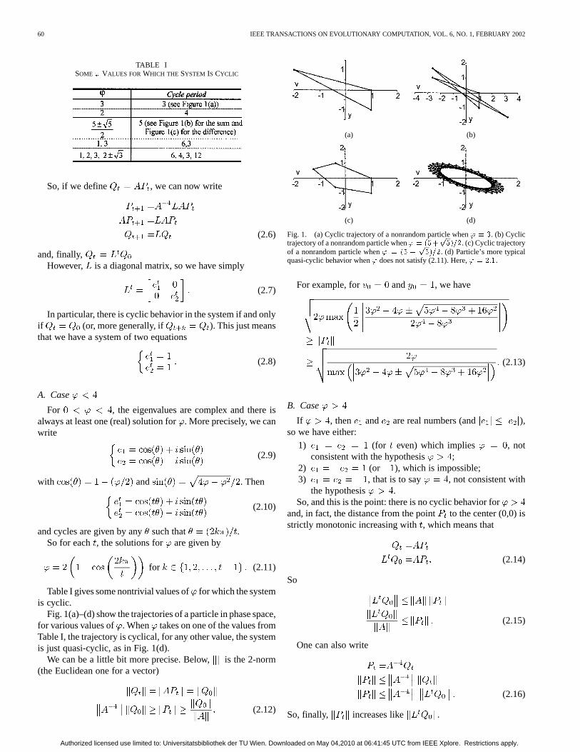
Fig. 1(a)–(d) show the trajectories of a particle in phase space,for various values of . When takes on one of the values fromTable I, the trajectory is cyclical, for any other value, the systemis just quasi-cyclic, as in Fig. 1(d).

We can be a little bit more precise. Below, is the 2-norm(the Euclidean one for a vector)

(2.12)

(a) (b)

(c) (d)

Fig. 1. (a) Cyclic trajectory of a nonrandom particle when' = 3. (b) Cyclictrajectory of a nonrandom particle when' = (5+

p5)=2. (c) Cyclic trajectory

of a nonrandom particle when' = (5 �p5)=2. (d) Particle’s more typical

quasi-cyclic behavior when' does not satisfy (2.11). Here,' = 2:1.

For example, for and , we have

(2.13)

B. Case

If , then and are real numbers (and ),so we have either:

1) (for even) which implies , notconsistent with the hypothesis ;

2) (or ), which is impossible;3) , that is to say , not consistent with

the hypothesis .So, and this is the point: there is no cyclic behavior for

and, in fact, the distance from the point to the center (0,0) isstrictly monotonic increasing with, which means that

(2.14)

So

(2.15)

One can also write

(2.16)

So, finally, increases like .



In Section IV, this result is used to prevent the explosion ofthe system, which can occur when particle velocities increasewithout control.

C. Case

In this situation

In this particular case, the eigenvalues are both equal toand there is just one family of eigenvectors, generated by

So, we have .Thus, if is an eigenvector, proportional to(that is to say,

if ), there are just two symmetrical points, for

(2.17)

In the case where is not an eigenvector, we can directlycompute how decreases and/or increases.

Let us define . By recurrence, thefollowing form is derived:

(2.18)

where , , are integers so that for .The integers can be negative, zero, or positive.

Supposing for a particularwe have , one can easilycompute . This quantity is pos-itive if and only if is not between (or equal to) the roots

.Now, if is computed, then we have

and the roots are .As , this result means that is also positive.So, as soon as begins to increase, it does so infinitely, butit can decrease, at the beginning. The question to be answerednext is, how long can it decrease before it begins increasing?

Now take the case of . This means that is betweenand . For instance, in the case where 1

with (2.19)

By recurrence, the following is derived:

with

(2.20)

Finally

(2.21)

1Note that the present paper uses the Bourbaki convention of representingopen intervals with reversed brackets. Thus, ]a,b[ is equivalent to parentheticalnotation (a,b).

as long as , which means that de-creases as long as

Integerpart (2.22)

After that, increases.The same analysis can be performed for . In this case,

, as well, so the formula is the same. In fact, to be evenmore precise, if

then we have

(2.23)

Thus, it can be concluded that decreases/increases al-most linearly when is big enough. In particular, even if itbegins to decrease, after that it tends to increase almost like

.

III. A NALYTIC POINT OF VIEW

A. Basic Explicit Representation

From the basic iterative (implicit) representation, the fol-lowing is derived:

(3.1)

Assuming a continuous process, this becomes a classicalsecond-order differential equation

(3.2)

where and are the roots of

(3.3)

As a result

(3.4)

The general solution is

(3.5)

A similar kind of expression for is now produced, where

(3.6)



The coefficients and depend on and . If, we have

(3.7)

In the case where , (3.5) and (3.6) give

(3.8)

so we must have

(3.9)

in order to prevent a discontinuity.Regarding the expressions and , eigenvalues of the ma-

trix , as in Section II above, the same discussion about thesign of ( ) can be made, particularly about the (non) ex-istence of cycles.

The above results provide a guideline for preventing the ex-plosion of the system, for we can immediately see that it dependson whether we have

(3.10)

B. A Posteriori Proof

One can directly verify that and are, indeed, solu-tions of the initial system.

On one hand, from their expressions

(3.11)

and on the other hand

(3.12)

and also

(3.13)

C. General Implicit and Explicit Representations

A more general implicit representation (IR) is produced byadding five coefficients , which will allow us toidentify how the coefficients can be chosen in order to ensureconvergence. With these coefficients, the system becomes

(3.14)

The matrix of the system is now

Let and be its eigenvalues.The (analytic) explicit representation (ER) becomes

(3.15)

with

(3.16)

Now the constriction coefficients (see Section IV for details)and are defined by

(3.17)

with

(3.18)

which are the eigenvalues of the basic system. By computingthe eigenvalues directly and using (3.17),and are

(3.19)



The final complete ER can then be written from (3.15) and(3.16) by replacing and , respectively, by andand then , , , by their expressions, as seen in (3.18)and (3.19).

It is immediately worth noting an important difference be-tween IR and ER. In the IR,is always an integer and and

are real numbers. In the ER, real numbers are obtained ifand only if is an integer; nothing, however, prevents the assign-ment of any real positive value to, in which case andbecome true complex numbers. This fact will provide an elegantway of explaining the system’s behavior, by conceptualizing itin a 5-D space, as discussed in Section IV.

Note 3.1: If and are to be real numbers for a givenvalue, there must be some relations among the five real coef-

ficients . If the imaginary parts of and areset equal to zero, (3.20) is obtained, as shown at the bottom ofthe page, with

sign

sign

sign

sign

(3.21)

The two equalities of (3.20) can be combined and simplifiedas follows:

signsign

(3.22)

The solutions are usually not completely independent of. Inorder to satisfy these equations, a set of possible conditions is

(3.23)

However, these conditions are not necessary. For example,an interesting particular situation (studied below) exists where

. In this case, forany value and (3.20) is always satisfied.

D. From ER to IR

The ER will be useful to find convergence conditions. Nev-ertheless, in practice, the iterative form obtained from (3.19) isvery useful, as shown in (3.24) at the bottom of the page.

Although there are an infinity of solutions in terms of the fiveparameters , it is interesting to identify some par-ticular classes of solutions. This will be done in the next section.

E. Particular Classes of Solutions

1) Class 1 Model:The first model implementing the five-parameter generalization is defined by the following relations:

(3.25)

In this particular case, and are

(3.26)

An easy way to ensure real coefficients is to have. Under this additional condition, a class of solution is

simply given by

(3.27)

2) Class Model: A related class of model is defined bythe following relation:

(3.28)

The expressions in (3.29), shown at the bottom of the nextpage, for and are derived from (3.24).

If the condition is added, then

or (3.30)

Without this condition, one can choose a value for, for ex-ample, and a corresponding value ( ), which givea convergent system.

sign sign

sign sign(3.20)

(3.24)



3) Class Model: A second model related to the Class 1formula is defined by

(3.31)

(3.32)

For historical reasons and for its simplicity, the case hasbeen well studied. See Section IV-C for further discussion.

4) Class 2 Model:A second class of models is defined bythe relations

(3.33)

Under these constraints, it is clear that

(3.34)

which gives us and , respectively.Again, an easy way to obtain real coefficients for every

value is to have . In this case

(3.35)

In the case where , the following is obtained:

(3.36)

From the standpoint of convergence, it is interesting to notethat we have the following.

1) For the Class 1 models, with the condition

(3.37)

2) For the Class models, with the conditionsand

(3.38)

3) For the the Class 2 models, see (3.39) at the bottom of thepage, with .

This means that we will just have to choose ,, and , class , respectively, to have a

convergent system. This will be discussed further in Section IV.

F. Removing the Discontinuity

Depending on the parameters the systemmay have a discontinuity in due to the presence of the term

in the eigen-values.

Thus, in order to have a completely continuous system, thevalues for must be chosen such that

(3.40)

By computing the discriminant, the last condition is found tobe equivalent to

(3.41)

In order to be “physically plausible,” the parametersmust be positive. So, the condition becomes

(3.42)

The set of conditions taken together specify a volume infor the admissible values of the parameters.

G. Removing the Imaginary Part

When the condition specified in (3.42) is met, the trajectoryis usually still partly in a complex space whenever one of theeigenvalues is negative, due to the fact that is a complex

(3.29)

(3.39)



number when is not an integer. In order to prevent this, wemust find some stronger conditions in order to maintain positiveeigenvalues.

Since

(3.43)

the following conditions can be used to ensure positive eigen-values:

(3.44)

Note 3.2: From an algebraic point of view, the conditionsdescribed in (3.43) can be written as

trace(3.45)

Now, these conditions depend on. Nevertheless, if the max-imum value is known, they can be rewritten as

(3.46)

Under these conditions, all system variables are real numbersin conjunction with the conditions in (3.42) and (3.44), the pa-rameters can be selected so that the system is completely con-tinuousand real.

H. Example

As an example, suppose that and . Now theconditions become

(3.47)

For example, when

(3.48)

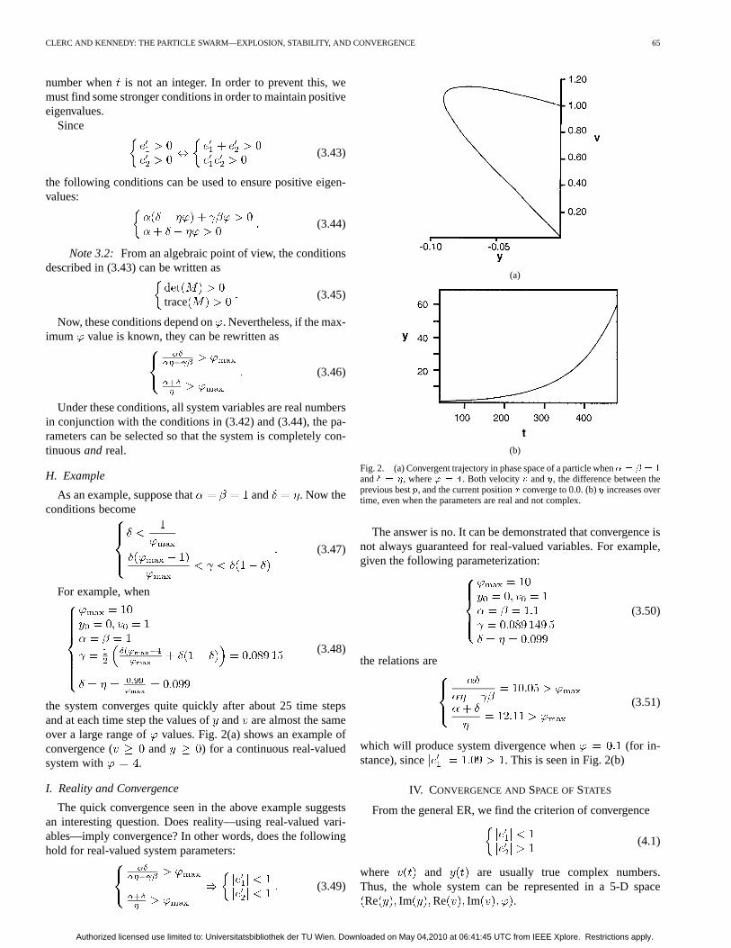
the system converges quite quickly after about 25 time stepsand at each time step the values ofand are almost the sameover a large range of values. Fig. 2(a) shows an example ofconvergence ( and ) for a continuous real-valuedsystem with .

I. Reality and Convergence

The quick convergence seen in the above example suggestsan interesting question. Does reality—using real-valued vari-ables—imply convergence? In other words, does the followinghold for real-valued system parameters:

(3.49)

(a)

(b)

Fig. 2. (a) Convergent trajectory in phase space of a particle when� = � = 1

and� = �, where' = 4. Both velocityv andy, the difference between theprevious bestp, and the current positionx converge to 0.0. (b)y increases overtime, even when the parameters are real and not complex.

The answer is no. It can be demonstrated that convergence isnot always guaranteed for real-valued variables. For example,given the following parameterization:

(3.50)

the relations are

(3.51)

which will produce system divergence when (for in-stance), since . This is seen in Fig. 2(b)

IV. CONVERGENCE ANDSPACE OFSTATES

From the general ER, we find the criterion of convergence

(4.1)

where and are usually true complex numbers.Thus, the whole system can be represented in a 5-D spaceRe Im Re Im .



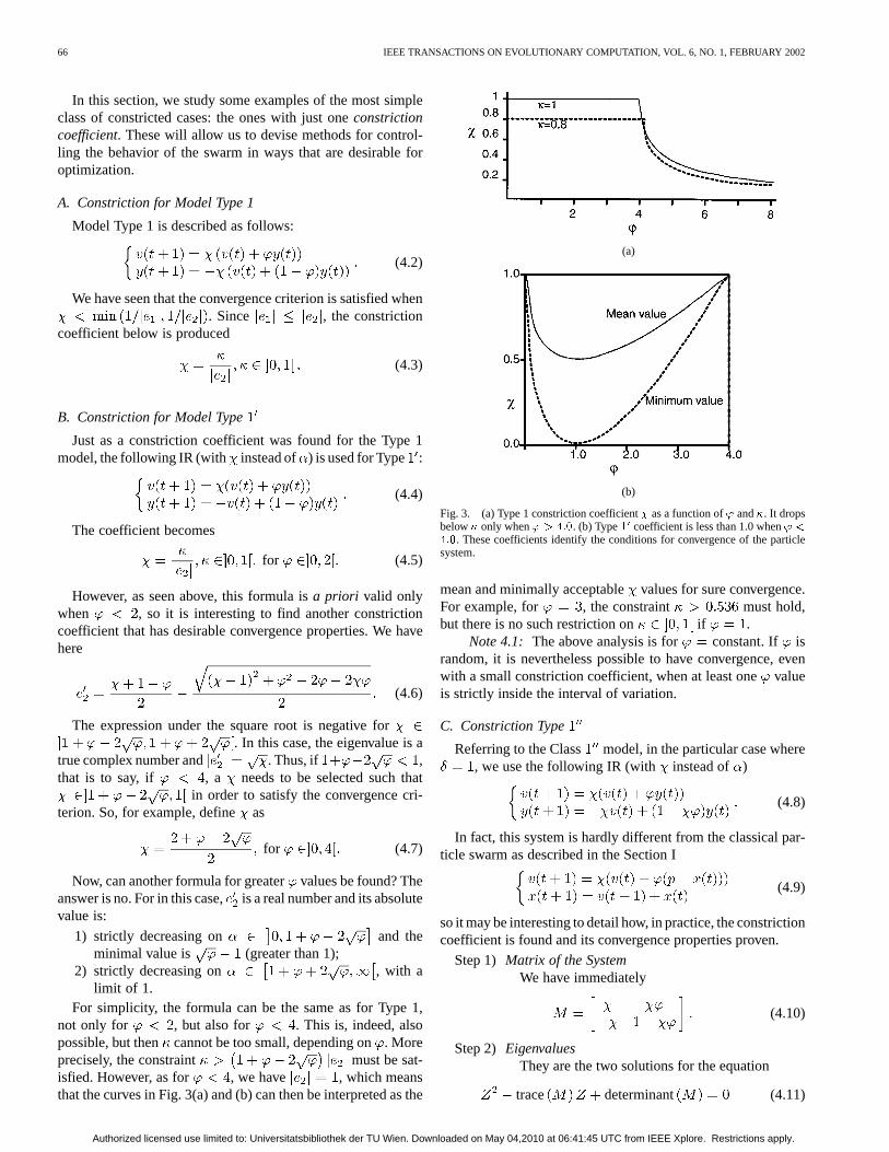
In this section, we study some examples of the most simpleclass of constricted cases: the ones with just oneconstrictioncoefficient. These will allow us to devise methods for control-ling the behavior of the swarm in ways that are desirable foroptimization.

A. Constriction for Model Type 1

Model Type 1 is described as follows:

(4.2)

We have seen that the convergence criterion is satisfied when. Since , the constriction

coefficient below is produced

(4.3)

B. Constriction for Model Type

Just as a constriction coefficient was found for the Type 1model, the following IR (with instead of ) is used for Type :

(4.4)

The coefficient becomes

for (4.5)

However, as seen above, this formula isa priori valid onlywhen , so it is interesting to find another constrictioncoefficient that has desirable convergence properties. We havehere

(4.6)

The expression under the square root is negative for. In this case, the eigenvalue is a

true complex number and . Thus, if ,that is to say, if , a needs to be selected such that

in order to satisfy the convergence cri-terion. So, for example, define as

for (4.7)

Now, can another formula for greatervalues be found? Theanswer is no. For in this case,is a real number and its absolutevalue is:

1) strictly decreasing on and theminimal value is (greater than 1);

2) strictly decreasing on , with alimit of 1.

For simplicity, the formula can be the same as for Type 1,not only for , but also for . This is, indeed, alsopossible, but then cannot be too small, depending on. Moreprecisely, the constraint must be sat-isfied. However, as for , we have , which meansthat the curves in Fig. 3(a) and (b) can then be interpreted as the

(a)

(b)

Fig. 3. (a) Type 1 constriction coefficient� as a function of' and�. It dropsbelow� only when' > 4:0. (b) Type1 coefficient is less than 1.0 when' <

4:0. These coefficients identify the conditions for convergence of the particlesystem.

mean and minimally acceptablevalues for sure convergence.For example, for , the constraint must hold,but there is no such restriction on if .

Note 4.1: The above analysis is for constant. If israndom, it is nevertheless possible to have convergence, evenwith a small constriction coefficient, when at least onevalueis strictly inside the interval of variation.

C. Constriction Type

Referring to the Class model, in the particular case where, we use the following IR (with instead of )

(4.8)

In fact, this system is hardly different from the classical par-ticle swarm as described in the Section I

(4.9)

so it may be interesting to detail how, in practice, the constrictioncoefficient is found and its convergence properties proven.

Step 1) Matrix of the SystemWe have immediately

(4.10)

Step 2) EigenvaluesThey are the two solutions for the equation

trace determinant (4.11)



or

(4.12)

Thus

(4.13)

with

trace determinant

(4.14)

Step 3) Complex and Real Areas onThe discriminant is negative for the values in

. Inthis area, the eigenvalues are true complex numbersand their absolute value (i.e., module) is simply.

Step 4) Extension of the Complex Region and ConstrictionCoefficient

In the complex region, according to the conver-gence criterion, in order to get convergence.So the idea is to find a constriction coefficient de-pending on so that the eigenvalues are true com-plex numbers for a large field of values. In thiscase, the common absolute value of the eigenvaluesis

for

else(4.15)

which is smaller than one for all values as soon asis itself smaller than one.

This is generally the most difficult step and sometimes needssome intuition. Three pieces of information help us here:

1) the determinant of the matrix is equal to;2) this is the same as in Constriction Type 1;3) we know from the algebraic point of view the system is

(eventually) convergent like .So it appears very probable that the same constriction coeffi-

cient used for Type 1 will work. First, we try

(4.16)

that is to say

for

else(4.17)

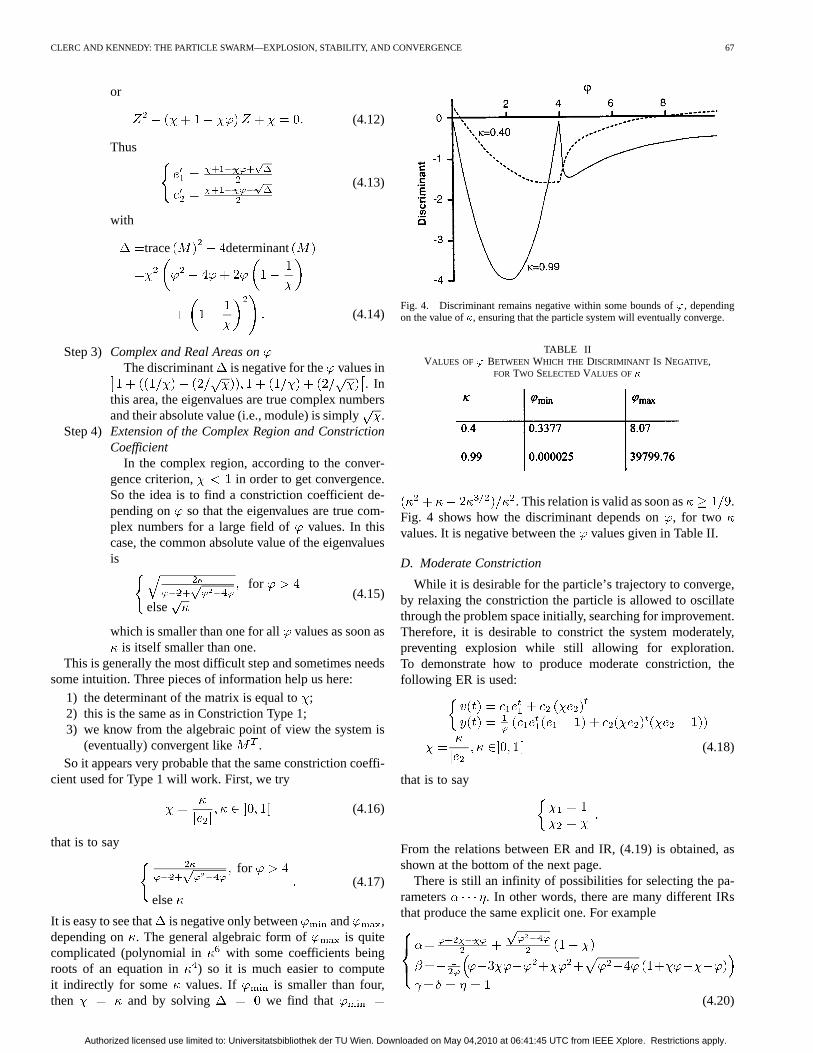
It is easy to see that is negative only between and ,depending on . The general algebraic form of is quitecomplicated (polynomial in with some coefficients beingroots of an equation in ) so it is much easier to computeit indirectly for some values. If is smaller than four,then and by solving we find that

Fig. 4. Discriminant remains negative within some bounds of', dependingon the value of�, ensuring that the particle system will eventually converge.

TABLE IIVALUES OF' BETWEEN WHICH THE DISCRIMINANT IS NEGATIVE,

FOR TWO SELECTED VALUES OF�

. This relation is valid as soon as .Fig. 4 shows how the discriminant depends on, for twovalues. It is negative between thevalues given in Table II.

D. Moderate Constriction

While it is desirable for the particle’s trajectory to converge,by relaxing the constriction the particle is allowed to oscillatethrough the problem space initially, searching for improvement.Therefore, it is desirable to constrict the system moderately,preventing explosion while still allowing for exploration.To demonstrate how to produce moderate constriction, thefollowing ER is used:

(4.18)

that is to say

From the relations between ER and IR, (4.19) is obtained, asshown at the bottom of the next page.

There is still an infinity of possibilities for selecting the pa-rameters . In other words, there are many different IRsthat produce the same explicit one. For example

(4.20)



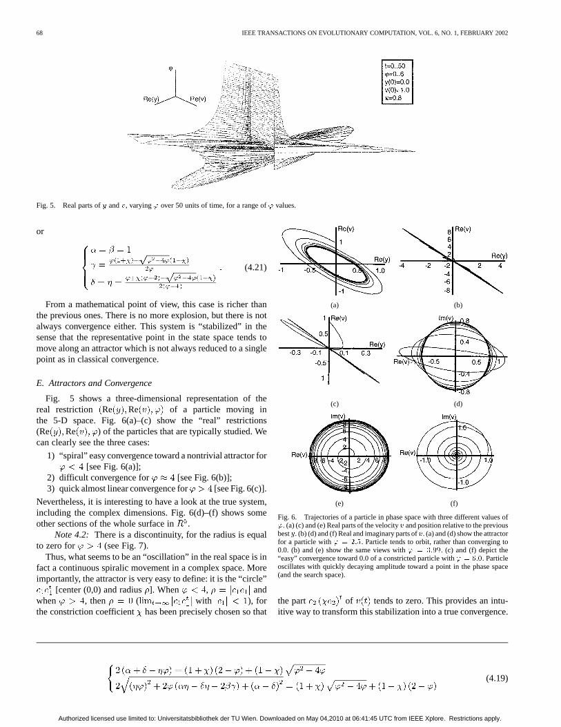
Fig. 5. Real parts ofy andv, varying' over 50 units of time, for a range of' values.

or

(4.21)

From a mathematical point of view, this case is richer thanthe previous ones. There is no more explosion, but there is notalways convergence either. This system is “stabilized” in thesense that the representative point in the state space tends tomove along an attractor which is not always reduced to a singlepoint as in classical convergence.

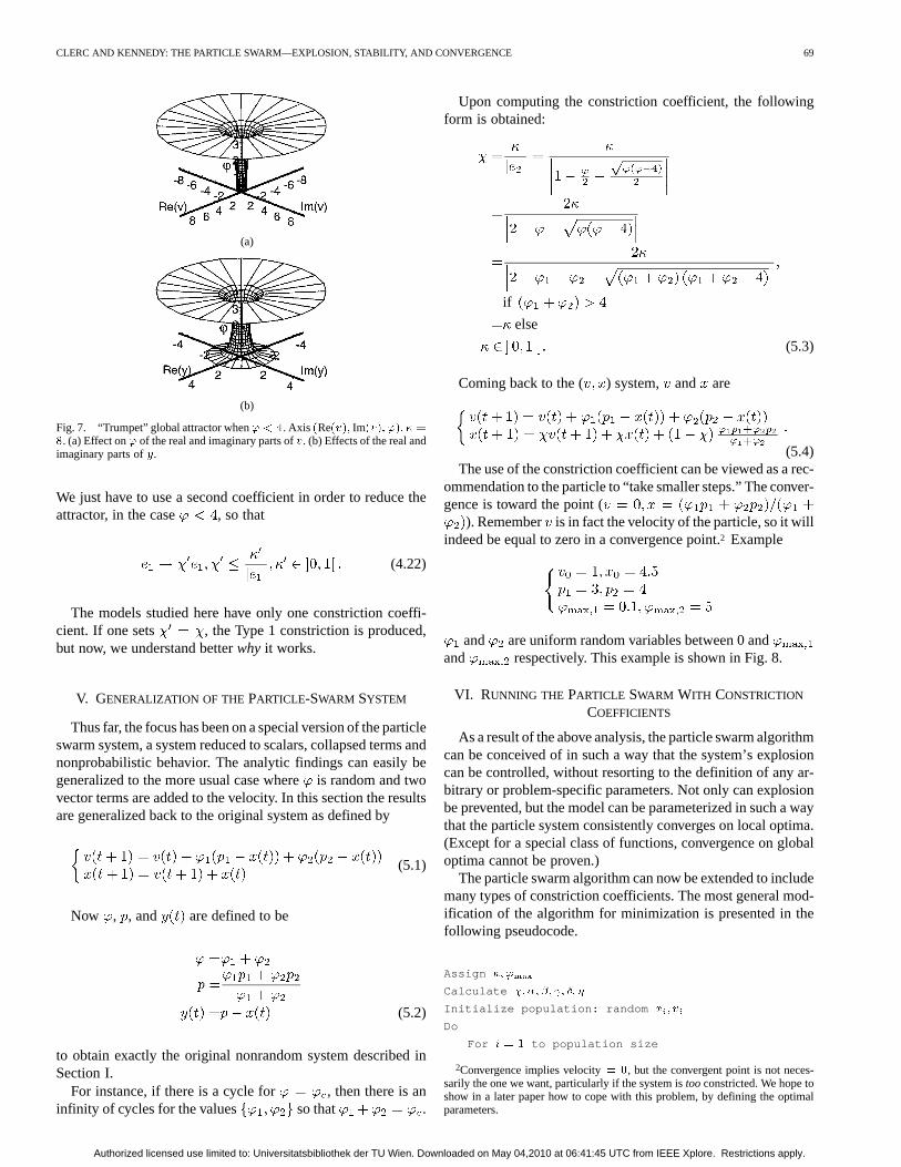
E. Attractors and Convergence

Fig. 5 shows a three-dimensional representation of thereal restriction Re Re of a particle moving inthe 5-D space. Fig. 6(a)–(c) show the “real” restrictions(Re Re ) of the particles that are typically studied. Wecan clearly see the three cases:

1) “spiral” easy convergence toward a nontrivial attractor for[see Fig. 6(a)];

2) difficult convergence for [see Fig. 6(b)];3) quick almost linear convergence for [see Fig. 6(c)].

Nevertheless, it is interesting to have a look at the true system,including the complex dimensions. Fig. 6(d)–(f) shows someother sections of the whole surface in.

Note 4.2: There is a discontinuity, for the radius is equalto zero for (see Fig. 7).

Thus, what seems to be an “oscillation” in the real space is infact a continuous spiralic movement in a complex space. Moreimportantly, the attractor is very easy to define: it is the “circle”

[center (0,0) and radius]. When , andwhen , then ( with ), forthe constriction coefficient has been precisely chosen so that

(a) (b)

(c) (d)

(e) (f)

Fig. 6. Trajectories of a particle in phase space with three different values of'. (a) (c) and (e) Real parts of the velocityv and position relative to the previousbesty. (b) (d) and (f) Real and imaginary parts ofv. (a) and (d) show the attractorfor a particle with' = 2:5. Particle tends to orbit, rather than converging to0.0. (b) and (e) show the same views with' = 3:99. (c) and (f) depict the“easy” convergence toward 0.0 of a constricted particle with' = 6:0. Particleoscillates with quickly decaying amplitude toward a point in the phase space(and the search space).

the part of tends to zero. This provides an intu-itive way to transform this stabilization into a true convergence.

(4.19)



(a)

(b)

Fig. 7. “Trumpet” global attractor when' < 4. Axis (Re(v); Im(v); '); � =8. (a) Effect on' of the real and imaginary parts ofv. (b) Effects of the real andimaginary parts ofy.

We just have to use a second coefficient in order to reduce theattractor, in the case , so that

(4.22)

The models studied here have only one constriction coeffi-cient. If one sets , the Type 1 constriction is produced,but now, we understand betterwhy it works.

V. GENERALIZATION OF THE PARTICLE-SWARM SYSTEM

Thus far, the focus has been on a special version of the particleswarm system, a system reduced to scalars, collapsed terms andnonprobabilistic behavior. The analytic findings can easily begeneralized to the more usual case whereis random and twovector terms are added to the velocity. In this section the resultsare generalized back to the original system as defined by

(5.1)

Now , , and are defined to be

(5.2)

to obtain exactly the original nonrandom system described inSection I.

For instance, if there is a cycle for , then there is aninfinity of cycles for the values so that .

Upon computing the constriction coefficient, the followingform is obtained:

if

else

(5.3)

Coming back to the ( ) system, and are

(5.4)The use of the constriction coefficient can be viewed as a rec-

ommendation to the particle to “take smaller steps.” The conver-gence is toward the point (

). Remember is in fact the velocity of the particle, so it willindeed be equal to zero in a convergence point.2 Example

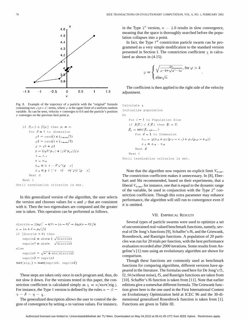
and are uniform random variables between 0 andand respectively. This example is shown in Fig. 8.

VI. RUNNING THE PARTICLE SWARM WITH CONSTRICTION

COEFFICIENTS

As a result of the above analysis, the particle swarm algorithmcan be conceived of in such a way that the system’s explosioncan be controlled, without resorting to the definition of any ar-bitrary or problem-specific parameters. Not only can explosionbe prevented, but the model can be parameterized in such a waythat the particle system consistently converges on local optima.(Except for a special class of functions, convergence on globaloptima cannot be proven.)

The particle swarm algorithm can now be extended to includemany types of constriction coefficients. The most general mod-ification of the algorithm for minimization is presented in thefollowing pseudocode.

Assign �; '

Calculate �;�; �; ; �; �

Initialize population: random x ; v

Do

For i = 1 to population size

2Convergence implies velocity= 0, but the convergent point is not neces-sarily the one we want, particularly if the system istooconstricted. We hope toshow in a later paper how to cope with this problem, by defining the optimalparameters.



Fig. 8. Example of the trajectory of a particle with the “original” formulacontaining two'(p�x) terms, where' is the upper limit of a uniform randomvariable. As can be seen, velocityv converges to 0.0 and the particle’s positionx converges on the previous best pointp.

if f(x ) < f(p ) then p = x

For d = 1 to dimension

'1 = rand () � (' =2)

'2 = rand () � (' =2)

' = '1 + '2

p = (('1 p ) + ('2 p ))='

x = x

v = v

v = � v + � ' (p� x)

x = p+ v � (� � (� ')) (p� x)

Next d

Next i

Until termination criterion is met.

In this generalized version of the algorithm, the user selectsthe version and chooses values forand that are consistentwith it. Then the two eigenvalues are computed and the greaterone is taken. This operation can be performed as follows.

discrim = ((�') � 4� + (�� ) + 2�'(�� ))=4

a = (�+ � � �')=2

if (discrim > 0) then

neprim 1 = abs (a +p

discrim )

neprim 2 = abs (a �p

discrim )

else

neprim 1 = a + abs (discrim )

neprim 2 = neprim 1

max(eig. ) = max(neprim 1; neprim 2)

These steps are taken only once in each program and, thus, donot slow it down. For the versions tested in this paper, the con-striction coefficient is calculated simply as eig. .For instance, the Type 1 version is defined by the rules

.The generalized description allows the user to control the de-

gree of convergence by settingto various values. For instance,

in the Type version, results in slow convergence,meaning that the space is thoroughly searched before the popu-lation collapses into a point.

In fact, the Type constriction particle swarm can be pro-grammed as a very simple modification to the standard versionpresented in Section I. The constriction coefficientis calcu-lated as shown in (4.15)

, for

else

The coefficient is then applied to the right side of the velocityadjustment.

Calculate �

Initialize population

Do

For i = 1 to Population Size

if f(~x ) < f(~p ) then ~p = ~x

~p = min(~p )

For d = 1 to Dimension

v = �(v + ' (p � x ) + ' (p � x ))

x = x + v

Next d

Next i

Until termination criterion is met.

Note that the algorithm now requires no explicit limit .The constriction coefficient makes it unnecessary. In [8], Eber-hart and Shi recommended, based on their experiments, that aliberal , for instance, one that is equal to the dynamic rangeof the variable, be used in conjunction with the Typecon-striction coefficient. Though this extra parameter may enhanceperformance, the algorithm will still run to convergence even ifit is omitted.

VII. EMPIRICAL RESULTS

Several types of particle swarms were used to optimize a setof unconstrained real-valued benchmark functions, namely, sev-eral of De Jong’s functions [9], Schaffer’s f6, and the Griewank,Rosenbrock, and Rastrigin functions. A population of 20 parti-cles was run for 20 trials per function, with the best performanceevaluation recorded after 2000 iterations. Some results from An-geline’s [1] runs using an evolutionary algorithm are shown forcomparison.

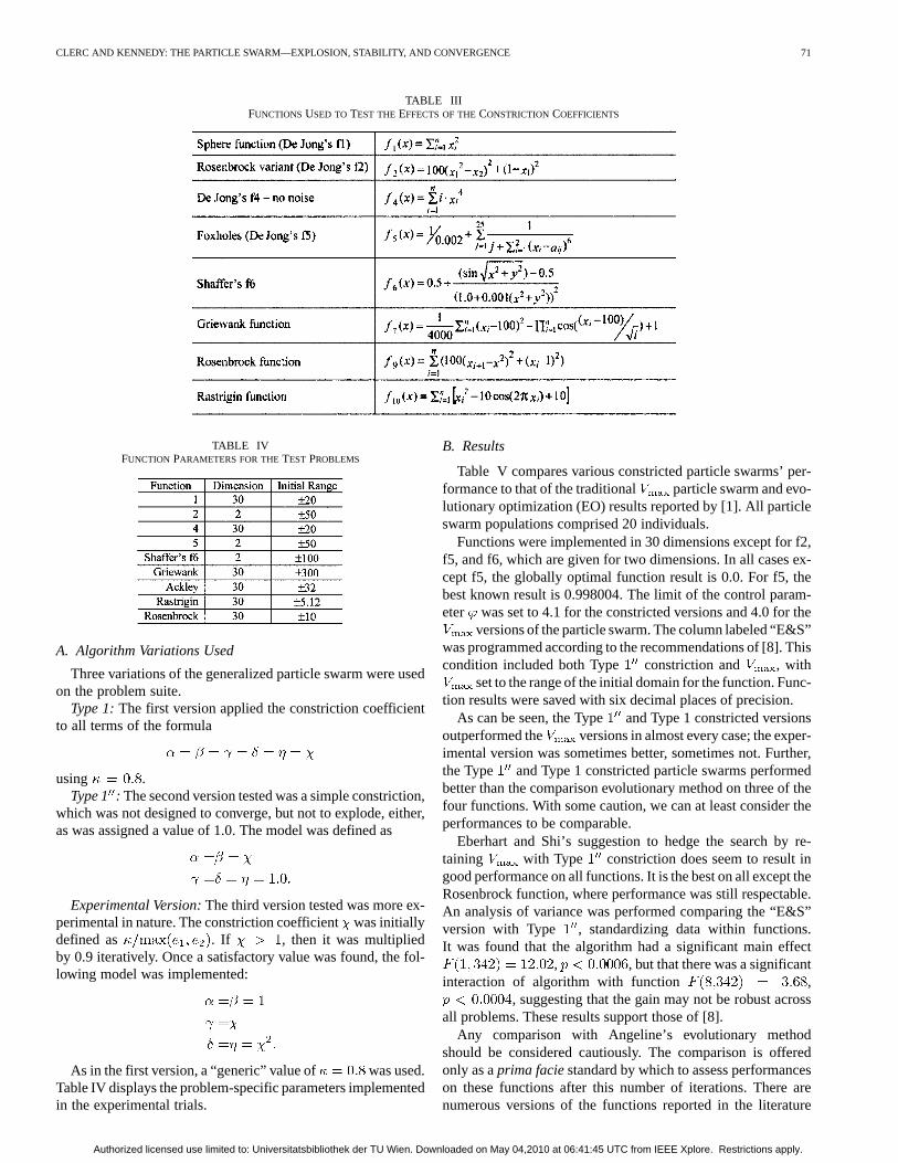
Though these functions are commonly used as benchmarkfunctions for comparing algorithms, different versions have ap-peared in the literature. The formulas used here for De Jong’s f1,f2, f4 (without noise), f5, and Rastrigin functions are taken from[10]. Schaffer’s f6 function is taken from [11]. Note that earliereditions give a somewhat different formula. The Griewank func-tion given here is the one used in the First International Conteston Evolutionary Optimization held at ICEC 96 and the 30-di-mensional generalized Rosenbrock function is taken from [1].Functions are given in Table III.



TABLE IIIFUNCTIONS USED TOTEST THEEFFECTS OF THECONSTRICTIONCOEFFICIENTS

TABLE IVFUNCTION PARAMETERS FOR THETEST PROBLEMS

A. Algorithm Variations Used

Three variations of the generalized particle swarm were usedon the problem suite.

Type 1:The first version applied the constriction coefficientto all terms of the formula

using .Type 1 : The second version tested was a simple constriction,

which was not designed to converge, but not to explode, either,as was assigned a value of 1.0. The model was defined as

Experimental Version:The third version tested was more ex-perimental in nature. The constriction coefficientwas initiallydefined as . If , then it was multipliedby 0.9 iteratively. Once a satisfactory value was found, the fol-lowing model was implemented:

As in the first version, a “generic” value of was used.Table IV displays the problem-specific parameters implementedin the experimental trials.

B. Results

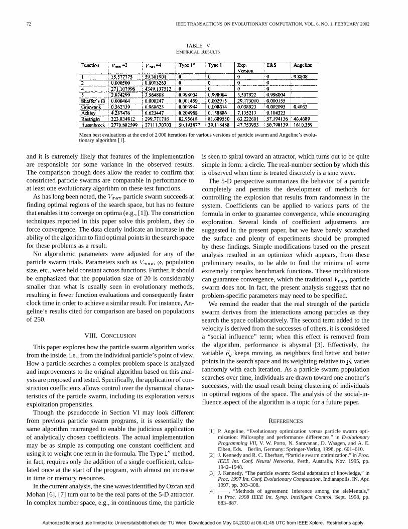
Table V compares various constricted particle swarms’ per-formance to that of the traditional particle swarm and evo-lutionary optimization (EO) results reported by [1]. All particleswarm populations comprised 20 individuals.

Functions were implemented in 30 dimensions except for f2,f5, and f6, which are given for two dimensions. In all cases ex-cept f5, the globally optimal function result is 0.0. For f5, thebest known result is 0.998004. The limit of the control param-eter was set to 4.1 for the constricted versions and 4.0 for the

versions of the particle swarm. The column labeled “E&S”was programmed according to the recommendations of [8]. Thiscondition included both Type constriction and , with

set to the range of the initial domain for the function. Func-tion results were saved with six decimal places of precision.

As can be seen, the Type and Type 1 constricted versionsoutperformed the versions in almost every case; the exper-imental version was sometimes better, sometimes not. Further,the Type and Type 1 constricted particle swarms performedbetter than the comparison evolutionary method on three of thefour functions. With some caution, we can at least consider theperformances to be comparable.

Eberhart and Shi’s suggestion to hedge the search by re-taining with Type constriction does seem to result ingood performance on all functions. It is the best on all except theRosenbrock function, where performance was still respectable.An analysis of variance was performed comparing the “E&S”version with Type , standardizing data within functions.It was found that the algorithm had a significant main effect

, , but that there was a significantinteraction of algorithm with function ,

, suggesting that the gain may not be robust acrossall problems. These results support those of [8].

Any comparison with Angeline’s evolutionary methodshould be considered cautiously. The comparison is offeredonly as aprima faciestandard by which to assess performanceson these functions after this number of iterations. There arenumerous versions of the functions reported in the literature



TABLE VEMPIRICAL RESULTS

Mean best evaluations at the end of 2 000 iterations for various versions of particle swarm and Angeline’s evolu-tionary algorithm [1].

and it is extremely likely that features of the implementationare responsible for some variance in the observed results.The comparison though does allow the reader to confirm thatconstricted particle swarms are comparable in performance toat least one evolutionary algorithm on these test functions.

As has long been noted, the particle swarm succeeds atfinding optimal regions of the search space, but has no featurethat enables it to converge on optima (e.g., [1]). The constrictiontechniques reported in this paper solve this problem, they doforce convergence. The data clearly indicate an increase in theability of the algorithm to find optimal points in the search spacefor these problems as a result.

No algorithmic parameters were adjusted for any of theparticle swarm trials. Parameters such as , , populationsize, etc., were held constant across functions. Further, it shouldbe emphasized that the population size of 20 is considerablysmaller than what is usually seen in evolutionary methods,resulting in fewer function evaluations and consequently fasterclock time in order to achieve a similar result. For instance, An-geline’s results cited for comparison are based on populationsof 250.

VIII. C ONCLUSION

This paper explores how the particle swarm algorithm worksfrom the inside, i.e., from the individual particle’s point of view.How a particle searches a complex problem space is analyzedand improvements to the original algorithm based on this anal-ysis are proposed and tested. Specifically, the application of con-striction coefficients allows control over the dynamical charac-teristics of the particle swarm, including its exploration versusexploitation propensities.

Though the pseudocode in Section VI may look differentfrom previous particle swarm programs, it is essentially thesame algorithm rearranged to enable the judicious applicationof analytically chosen coefficients. The actual implementationmay be as simple as computing one constant coefficient andusing it to weight one term in the formula. The Typemethod,in fact, requires only the addition of a single coefficient, calcu-lated once at the start of the program, with almost no increasein time or memory resources.

In the current analysis, the sine waves identified by Ozcan andMohan [6], [7] turn out to be the real parts of the 5-D attractor.In complex number space, e.g., in continuous time, the particle

is seen to spiral toward an attractor, which turns out to be quitesimple in form: a circle. The real-number section by which thisis observed when time is treated discretely is a sine wave.

The 5-D perspective summarizes the behavior of a particlecompletely and permits the development of methods forcontrolling the explosion that results from randomness in thesystem. Coefficients can be applied to various parts of theformula in order to guarantee convergence, while encouragingexploration. Several kinds of coefficient adjustments aresuggested in the present paper, but we have barely scratchedthe surface and plenty of experiments should be promptedby these findings. Simple modifications based on the presentanalysis resulted in an optimizer which appears, from thesepreliminary results, to be able to find the minima of someextremely complex benchmark functions. These modificationscan guarantee convergence, which the traditional particleswarm does not. In fact, the present analysis suggests that noproblem-specific parameters may need to be specified.

We remind the reader that the real strength of the particleswarm derives from the interactions among particles as theysearch the space collaboratively. The second term added to thevelocity is derived from the successes of others, it is considereda “social influence” term; when this effect is removed fromthe algorithm, performance is abysmal [3]. Effectively, thevariable keeps moving, as neighbors find better and betterpoints in the search space and its weighting relative tovariesrandomly with each iteration. As a particle swarm populationsearches over time, individuals are drawn toward one another’ssuccesses, with the usual result being clustering of individualsin optimal regions of the space. The analysis of the social-in-fluence aspect of the algorithm is a topic for a future paper.

REFERENCES

[1] P. Angeline, “Evolutionary optimization versus particle swarm opti-mization: Philosophy and performance differences,” inEvolutionaryProgramming VII, V. W. Porto, N. Saravanan, D. Waagen, and A. E.Eiben, Eds. Berlin, Germany: Springer-Verlag, 1998, pp. 601–610.

[2] J. Kennedy and R. C. Eberhart, “Particle swarm optimization,” inProc.IEEE Int. Conf. Neural Networks, Perth, Australia, Nov. 1995, pp.1942–1948.

[3] J. Kennedy, “The particle swarm: Social adaptation of knowledge,” inProc. 1997 Int. Conf. Evolutionary Computation, Indianapolis, IN, Apr.1997, pp. 303–308.

[4] , “Methods of agreement: Inference among the eleMentals,”in Proc. 1998 IEEE Int. Symp. Intelligent Control, Sept. 1998, pp.883–887.



[5] Y. Shi and R. C. Eberhart, “Parameter selection in particle swarm adap-tation,” in Evolutionary Programming VII, V. W. Porto, N. Saravanan,D. Waagen, and A. E. Eiben, Eds. Berlin, Germany: Springer-Verlag,1997, pp. 591–600.

[6] E. Ozcan and C. K. Mohanet al., “Analysis of a simple particle swarmoptimization problem,” inProc. Conf. Artificial Neural Networks inEngineering, C. Dagli et al., Eds., St. Louis, MO, Nov. 1998, pp.253–258.

[7] , “Particle swarm optimization: Surfing the waves,” inProc. 1999Congr. Evolutionary Computation, Washington, DC, July 1999, pp.1939–1944.

[8] R. C. Eberhart and Y. Shi, “Comparing inertia weights and constrictionfactors in particle swarm optimization,” inProc. 2000 Congr. Evolu-tionary Computation, San Diego, CA, July 2000, pp. 84–88.

[9] K. De Jong, “An analysis of the behavior of a class of genetic adaptivesystems,” Ph.D. dissertation, Dept. Comput. Sci., Univ. Michigan, AnnArbor, MI, 1975.

[10] R. G. Reynolds and C.-J. Chung, “Knowledge-based self-adaptation inevolutionary programming using cultural algorithms,” inProc. IEEEInt. Conf. Evolutionary Computation, Indianapolis, IN, Apr. 1997, pp.71–76.

[11] L. Davis, Ed.,Handbook of Genetic Algorithms. New York: Van Nos-trand Reinhold, 1991.

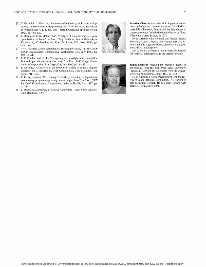
Maurice Clerc received the M.S. degree in mathe-matics (algebra and complex functions) from the Uni-versité de Villeneuve, France, and the Eng. degree incomputer science from the Institut industriel du Nord,Villeneuve d’Asq, France, in 1972.

He is currently with Research and Design, FranceTélécom, Annecy, France. His current research in-terests include cognitive science, nonclassical logics,and artificial intelligence.

Mr. Clerc is a Member of the French Associationfor Artificial Intelligence and the Internet Society.

James Kennedy received the Master’s degree inpsychology from the California State University,Fresno, in 1990 and the Doctorate from the Univer-sity of North Carolina, Chapel Hill, in 1992.

He is currently a Social Psychologist with the Bu-reau of Labor Statistics, Washington, DC, working indata collection research. He has been working withparticle swarms since 1994.


the particle swarm-explosion, stability, and convergence ... · the particle swarm—explosion,...

Documents