convergence analysis for particle swarm optimization … · · 2015-04-17isbn 978-3-944057-30-9...
TRANSCRIPT
FAU
UN
IVE
RS
ITY
PR
ES
S 2
015
ISBN 978-3-944057-30-9
UNIVERSITY P R E S S
Berthold Immanuel Schmitt
Convergence Analysis for Particle Swarm Optimization
Particle swarm optimization (PSO) is a very popular, randomized, nature- inspired meta-heuristic for solving continuous black box optimization problems. The main idea is to mimic the behavior of natural swarms like, e. g., bird flocks and fish swarms that find pleasant regions by sharing information. The movement of a particle is influenced not only by its own experience, but also by the experiences of its swarm members.In this thesis, we study the convergence process in detail. In order to mea- sure how far the swarm at a certain time is already converged, we define and analyze the potential of a particle swarm. This potential analysis leads to the proof that in a 1-dimensional situation, the swarm with probability 1 converges towards a local optimum for a comparatively wide range of objective functions. Additionally, we apply drift theory in order to prove that for unimodal objective functions the result of the PSO algorithm agrees with the actual optimum in 𝑘 digits after time 𝒪(𝑘).In the general D-dimensional case, it turns out that the swarm might not converge towards a local optimum. Instead, it gets stuck in a situation where some dimensions have a potential that is orders of magnitude smaller than others. Such dimensions with a too small potential lose their influence on the behavior of the algorithm, and therefore the respective entries are not optimized. In the end, the swarm stagnates, i. e., it converges towards a point in the search space that is not even a local optimum. In order to solve this issue, we propose a slightly modified PSO that again guarantees convergence towards a local optimum.
Ber
tho
ld Im
man
uel S
chm
itt
Con
verg
ence
Ana
lysi
s fo
r P
artic
le S
war
m O
ptim
izat
ion
FAU Forschungen, Reihe B, Medizin, Naturwissenschaft, Technik 3


Bibliografische Information der Deutschen Nationalbibliothek: Die Deutsche Nationalbibliothek verzeichnet diese Publikation in der Deutschen Nationalbibliografie; detaillierte bibliografische Daten sind im Internet über http://dnb.d-nb.de abrufbar. Das Werk, einschließlich seiner Teile, ist urheberrechtlich geschützt. Die Rechte an allen Inhalten liegen bei ihren jeweiligen Autoren. Sie sind nutzbar unter der Creative Commons Lizenz BY-NC-ND.
Der vollständige Inhalt des Buchs ist als PDF über den OPUS Server der Friedrich-Alexander-Universität Erlangen-Nürnberg abrufbar: http://opus.uni-erlangen.de/opus/
Verlag und Auslieferung:
FAU University Press, Universitätsstraße 4, 91054 Erlangen
Druck: docupoint GmbH
ISBN: 978-3-944057-30-9 ISSN: 2198-8102
Convergence Analysis for Particle
Swarm Optimization
Konvergenzanalyse für die Partikelschwarmoptimierung
Der Technischen Fakultät
der Friedrich-Alexander-Universität
Erlangen-Nürnberg
zur
Erlangung des Doktorgrades Dr.-Ing.
vorgelegt von
Berthold Immanuel Schmitt
aus Hildesheim

Als Dissertation genehmigt
von der Technischen Fakultät
der Friedrich-Alexander-Universität Erlangen-Nürnberg
Tag der mündlichen Prüfung: 04.02.2015
Vorsitzende des Promotionsorgans: Prof. Dr.-Ing. habil. Marion Merklein
Gutachter: Professor Dr. rer. nat. Rolf Wanka
Professor Dr. rer. nat. Benjamin Doerr

Abstract
Particle swarm optimization (PSO) is a very popular, randomized, nature-
inspiredmeta-heuristic for solving continuous black box optimization prob-
lems. The main idea is to mimic the behavior of natural swarms like, e. g.,
bird flocks and fish swarms, that find pleasant regions by sharing informa-
tion and cooperating rather than competing against each other. For opti-
mization purpose, a number of artificial particles move through the RD and
the movement of a particle is influenced not only by its own experience, but
also by the experiences of its swarm members.
Although this method is widely used in real-world applications, there is
unfortunately not much understanding of PSO based on formal analyses, ex-
plaining more than only partial aspects of the algorithm. One aspect that is
target of many researchers’ work is the phenomenon of a converging swarm,
i. e., the particles converge towards a single point in the search space. In
particular, necessary and sufficient conditions to the swarm parameters, i. e.,
certain parameters that control the behavior of the swarm, for guaranteeing
convergence could be derived. However, prior to this work, no theoretical re-
sult about the quality of this limit for the unmodified PSO algorithm and a
situation more general than considering just one particular objective func-
tion have been shown.
In this thesis, we study the convergence process in detail. In order to mea-
sure, how far the swarm at a certain time is already converged, we define and
analyze the potential of a particle swarm. The potential is constructed such
that it converges to 0 if and only if the swarm converges, but we will prove
that in the 1-dimensional case, when the swarm is far away from a local op-
timum, the potential increases. This observation turns out to be sufficient
to prove the first main result, namely that in a 1-dimensional situation, the
swarm with probability 1 converges towards a local optimum for a compar-
atively wide range of objective functions. Additionally, we apply drift theory
in order to prove that for unimodal objective functions, the result of the PSO
algorithm agrees with the actual optimum in k digits after time O(k).
iii
In the generalD-dimensional case, it turns out that the swarm might not
converge towards a local optimum. Instead, it gets stuck in a situation where
some dimensions have a potential orders of magnitude smaller than oth-
ers. Such dimensions with a too small potential lose their influence on the
behavior of the algorithm, and therefore, the respective entries are not op-
timized. In the end, the swarm stagnates, i. e., it converges towards a point
in the search space, that is not even a local optimum. In order to solve this
issue, we propose a slightly modified PSO that again guarantees convergence
towards a local optimum.
iv

Zusammenfassung
Partikelschwarmoptimierung (PSO) ist eine sehr verbreitete, randomisier-
te, von der Natur inspirierte Meta-Heuristik zum Lösen von Black-Box-Op-
timierungsproblemen über einem kontinuierlichen Suchraum. Die Grundi-
dee besteht in der Nachahmung des Verhaltens von in der Natur auftreten-
den Schwärmen, die vielversprechende Regionen finden, indem sie Informa-
tionen austauschen undmiteinander kooperieren, anstatt gegeneinander zu
konkurrieren. Im daraus gewonnenen Optimierungsverfahren bewegen sich
künstliche Partikel durch den RD, wobei die Bewegung eines Partikels nicht
nur von dessen eigener Erfahrung, sondern genauso von den Erfahrungen
der übrigen Schwarmmitglieder beeinflusst wird.
Obwohl diese Methode in zahlreichen realen Anwendungen verwendet
wird, haben theoretische Betrachtungen bisher nur einige wenige Teilaspek-
te des Algorithmus erklärt. Ein solcher Aspekt, mit dem sich viele Wissen-
schaftler auseinandersetzen, ist das Phänomen der Konvergenz des Partikel-
schwarms. Das bedeutet, dass die Partikel gegen einen Punkt im Suchraum
konvergieren. Insbesondere konnten notwendige und hinreichende Bedin-
gungen an die Schwarmparameter, bestimmte Parameter die das Verhalten
des Schwarms steuern, ermittelt werden, unter denen Konvergenz gewähr-
leistet ist. Allerdings ist bis jetzt kein theoretisches Resultat über dieQualität
dieses Grenzwertes bekannt, das für den unmodifizierten PSO-Algorithmus
in einer allgemeineren Situation als beispielsweise nur für genau eine Ziel-
funktion bewiesen werden konnte.
Diese Arbeit befasst sich detailliert mit dem Prozess der Konvergenz. Um
zu messen, wie stark der Schwarm bereits konvergiert ist, wird das Potential
eines Partikelschwarms eingeführt und analysiert. Das Potential ist so kon-
struiert, dass es genau dann gegen 0 konvergiert, wenn der Schwarm kon-
vergiert. Im 1-dimensionalen Fall ergeben die Betrachtungen, dass sich das
Potential erhöht, solange der Schwarmweit vom nächsten lokalen Optimum
entfernt ist. Diese Beobachtung führt zum Beweis des ersten Hauptresul-
tats, nämlich dass im 1-dimensionalen Fall der Schwarm fast sicher gegen
ein lokales Optimum konvergiert. Dieses Resultat ist für eine vergleichbar
v

große Klasse von Zielfunktionen gültig. Zusätzlich kann mittels Drifttheorie
gezeigt werden, dass das Ergebnis des PSO-Algorithmus nach einer Zeit von
O(k) mit dem tatsächlichen Optimum in k Bits übereinstimmt.
Im allgemeinenD-dimensionalen Fall stellt sich heraus, dass der Schwarm
nicht zwangsläufig gegen ein lokalesOptimumkonvergiert. Stattdessen gerät
er in eine Situation, in der manche Dimensionen ein um Größenordnungen
geringeres Potential haben als andere. Diese Dimensionen mit zu geringem
Potential verlieren ihren Einfluss auf das Verhalten des Algorithmus, und da-
herwerden die entsprechenden Einträge nicht optimiert. Die Konsequenz ist
Stagnation des Schwarms, das heißt, der Schwarm konvergiert gegen einen
Punkt im Suchraum, der nicht mal ein lokales Optimum ist. Um dieses Pro-
blem zu lösen wird eine leicht modifizierte Version der PSO vorgeschlagen,
die wiederum eine Garantie für Konvergenz gegen ein lokales Optimum zu-
lässt.
vi
"The PSO algorithm can be compared to a group of nerdsrandomly spread in the mountains. They are supposed to get
close to the highest point in a limited area. As nerds usually arenot used to daylight, their only way to navigate is via the GPS in
their mobile phones. Furthermore, they are allowed to usefacebook to share their position with their friends. Now they walk
randomly around, always a bit towards their personal previousbest position and a bit towards the best position on facebook."
Christoph Strößner, participant of Sarntal Ferienakademie, 2014
vii


Acknowledgments
First of all, I would like to expressmy sincere gratitude to Prof. Dr. RolfWanka
for his supervision, support and editorial and scientific advice throughout
the whole time of my graduate studies.
Additionally, I am grateful to the staff of the chair of Hardware-Software-
Co-Design for the great and interesting time I had there.
Special thanks for their great work and the interesting discussions go to
the students whose bachelor andmaster theses I supervised, namely Vanessa
Lange, Bernd Bassimir, Franz Köferl, Stefan Ploner, Lydia Schwab, Alexander
Raß and Gabriel Herl.
Finally, I would like to thankmy colleague and office roommateDr.-Ing.Mo-
ritz Mühlenthaler for the great years, for many exchanged ideas and for care-
fully reading wide parts of this thesis.
ix


Contents
1 Introduction and Contribution 11.1 Contributions . . . . . . . . . . . . . . . . . . . . . . . . . . 2
1.2 Overview . . . . . . . . . . . . . . . . . . . . . . . . . . . . . 6
2 Particle Swarm Optimization: State of the Art 92.1 Applications of Particle Swarm Optimization . . . . . . . . . 10
2.2 The Classical Particle Swarm Optimization Algorithm . . . . 12
2.3 Variants of Particle Swarm Optimization . . . . . . . . . . . 16
2.3.1 Neighborhood Topologies . . . . . . . . . . . . . . . . 16
2.3.2 Constraints and Bound Handling . . . . . . . . . . . 21
2.3.3 Variants of the Movement Equations . . . . . . . . . 25
2.4 Multi-Objective Particle Swarm Optimization . . . . . . . . 31
2.4.1 Multi-Objective Black Box Optimization . . . . . . . 31
2.4.2 PSO for Multi-Objective Black Box Optimization . . 33
2.5 Particle Swarm Optimization for Discrete Problems . . . . . 36
2.6 Theoretical Results about Particle Swarm Optimization . . . 38
2.7 Other Nature-Inspired Meta-Heuristics . . . . . . . . . . . . 41
2.7.1 Evolutionary Algorithms . . . . . . . . . . . . . . . . 41
2.7.2 Ant Algorithms . . . . . . . . . . . . . . . . . . . . . 45
3 PSO as a Stochastic Process 493.1 Basics of Probability Theory . . . . . . . . . . . . . . . . . . 50
3.1.1 Probability Space, Random Variables, Stochastic Pro-
cesses and Conditional Expectation . . . . . . . . . . 50
3.1.2 Measurability . . . . . . . . . . . . . . . . . . . . . . 58
3.2 (No) Free Lunch and Lebesgue’s Differentiation Theorem . . 60
3.3 Drift Theory . . . . . . . . . . . . . . . . . . . . . . . . . . . 61
3.3.1 Classical Drift Theory . . . . . . . . . . . . . . . . . . 62
3.3.2 Drift Theory for Continuous Search Spaces . . . . . . 63
3.4 The PSO Model . . . . . . . . . . . . . . . . . . . . . . . . . 71
xi

Contents
3.5 Discussion of Previous Results . . . . . . . . . . . . . . . . . 74
3.5.1 Negative Results . . . . . . . . . . . . . . . . . . . . . 74
3.5.2 Convergence Analysis . . . . . . . . . . . . . . . . . . 77
4 Convergence of 1-dimensional PSO 814.1 Particle SwarmOptimizationAlmost Surely Finds LocalOptima 81
4.1.1 Proof of Convergence Towards a Local Optimum . . . 84
4.1.2 Experimental Setup . . . . . . . . . . . . . . . . . . . 93
4.1.3 Experimental Results on the Potential gain . . . . . . 94
4.2 Proof of Linear Convergence Time . . . . . . . . . . . . . . . 96
4.2.1 Measuring the Distance to Optimality . . . . . . . . . 96
4.2.2 Lower Bounds for the Decrease of the Distance Measure 101
4.2.3 Putting things together . . . . . . . . . . . . . . . . . 137
5 Convergence for Multidimensional Problems 1455.1 Determining Further Bad Events . . . . . . . . . . . . . . . . 146
5.1.1 High Potential in at least one Dimension: A Bad Event 147
5.1.2 Low Potential in every Dimension: A Bad Event . . . 151
5.1.3 Imbalanced Potentials: A Fatal Event . . . . . . . . . 156
5.2 Modified Particle Swarm Optimization Almost Surely Finds
Local Optima . . . . . . . . . . . . . . . . . . . . . . . . . . . 175
5.3 Experimental Results with a Standard Implementation . . . 180
5.3.1 The Problem of Imbalanced Potentials on Standard
Benchmarks . . . . . . . . . . . . . . . . . . . . . . . 180
5.3.2 Avoiding Imbalanced Convergence . . . . . . . . . . . 182
5.3.3 Differentiability . . . . . . . . . . . . . . . . . . . . . 183
5.3.4 Impact of the Modification . . . . . . . . . . . . . . . 186
6 Conclusion 189
Bibliography 191
Author’s Own Publications 209
Acronyms 211
Index 213
xii
1. Introduction and Contribution
Particle swarmoptimization (PSO), originally invented byKennedy andEber-
hart [KE95, EK95] in 1995, is a very popular nature-inspired meta-heuristic
for solving continuous optimization problems. It is designed to reflect the
social interaction of individuals living together in groups and supporting
and cooperating with each other, rather than competing against each other.
Fields of successful application are Biomedical Image Processing [WSZ+04],
Geosciences [OD10],Mechanical Engineering [GWHK09], andMaterials Sci-
ence [RPPN09], to name just a few, where the continuous objective function
on a multi-dimensional domain is not given in a closed form, but by a “black
box.” That means that the only operation that the objective function allows
is the evaluation of search points while, e. g., gradient information is not
available.
The popularity of the PSO framework in various scientific communities
is due to the fact that it on the one hand can be realized and, if necessary,
adapted to further needs easily, but on the other hand shows in experiments
good performance results with respect to the quality of the obtained solution
and the time needed to obtain it. By adapting its parameters, users may in
real-world applications easily and successfully control the swarm’s behavior
with respect to “exploration” (“searching where no one has searched before”)
and “exploitation” (“searching around a good position”). A thorough discus-
sion of PSO can be found in [PSL11].
To be precise, let an objective function f : RD → R on a D-dimensional
domain be given that (without loss of generality) has to be minimized. A
population of particles, each consisting of a position (the candidate for a
solution), a velocity and a local attractor, moves through the search space
RD. The local attractor of a particle is the best position with respect to f
this particle has encountered so far. The population in motion is the swarm.
In contrast to evolutionary algorithms, the individuals of the swarm coop-
erate by sharing information about the search space via the global attractor,
which is the best position any particle has found so far. The particles move
in time-discrete iterations. The movement of a particle is governed by so-
1

1. Introduction and Contribution
called movement equations that depend on both the particle’s velocity and
its two attractors and on some additional fixed parameters, controlling the
influence of the attractors and the velocity on the next step (for details, see
Chapter 2.2).
Although this method is widely used in real-world applications, there is
unfortunately not much understanding of the algorithm based on formal
analyses, explaining more than only partial aspects like analyzing the trajec-
tories of restricted and deterministic PSO variants. One aspect that is target
of many researchers’ work is the phenomenon of a converging swarm, i. e.,
the particles converge towards one point in the search space. This exploita-
tive behavior is desired because it allows the swarm to refine a solution and
maybe come arbitrarily close to the optimum. Many experiments support
the claim that using appropriate parameters allows the swarm to converge.
In particular, necessary and sufficient conditions to the swarm parameters
were derived in the literature, which guarantee convergence of the swarm
under the assumption that the attractors are constant. However, until now,
no theoretical result about the quality of this limit for the unmodified PSO
algorithm, valid in a situation more general than considering just one par-
ticular objective function, have been shown.
1.1 Contributions
Themain goal of this thesis is to provide the first generalmathematical anal-
ysis of the quality of the global attractor when it is considered as a solution
for objective functions from a very general class F of functions and there-
fore of the quality of the algorithm’s return value. The set F consists of all
functions that have a continuous first derivative and, roughly spoken, have
only a bounded area that is of interest for the particles. Note that the class
F of admissible objective functions, for which our convergence results hold,
is much more general than, e. g., the subset of the class of the unimodal
functions that is considered in [Jäg07] in the context of restricted (1 + 1)evolutionary algorithms.
First, we propose a mathematically sound model of PSO, which describes
the algorithm as a stochastic process over the real numbers. Before present-
ing our convergence analysis, several previous results, in particular different
2
1.1 Contributions
negative results stating that the PSO algorithm is not an “optimizer”, are dis-
cussed in the light of this new model.
Main Tools for the Analysis
As an important tool for the analysis, we introduce the new approach of
defining the potential of the particle swarm that changes after every step.
The potential covers two properties of the swarm: It tends to 0 if the par-
ticles converge, but we can show that it increases if the whole swarm stays
close to a search point that is no local minimum. In the latter case, we prove
that the swarm charges potential and resumes its movement.
Another important tool for our analysis is drift theory, which has already
been used for proving runtime bounds in the area of evolutionary algorithms.
Drift theorems allow us to transform bounds of the drift, i. e., the expected
tendency of a stochastic process in a certain direction, into bounds on the
expected time until the process hits a predefined value. In order to use
drift theory for analyzing PSO, we formulate and prove a new drift theorem,
specifically designed for stochastic processes on the continuous domain R.As far as we know, this thesis contains the first work that analyzes PSO with
the help of drift theory.
Contributions to the Analysis of 1-Dimensional PSO
As our first main result, we can prove an emergent property of PSO for F,namely that in the 1-dimensional case the swarm almost surely (in the well-
defined probabilistic sense) finds a local optimum. More precisely: If no
two local optima have the same objective function value, then the swarm
converges towards a local optimum almost surely.
Since the possible area for the global attractor is bounded, the Bolzano-
Weierstrass theorem implies that either the global attractor converges to-
wards a single point in the search space, or there are at least two accumula-
tion points of the global attractor, i. e., points to which the global attractor
comes arbitrarily close infinitely often. If the global attractor converges, then
the results of previous theoretical work guarantee convergence of the whole
3

1. Introduction and Contribution
swarm. But, as our potential analysis shows, the swarm cannot converge to-
wards a point that is no local optimum. So, if the global attractor converges,
then its limit is a local optimum. If there are two or more accumulation
points, then the swarmmaintains a certain amount of potentential, depend-
ing on the distance between the accumulation points, since this distance is
overcome infinitely often. As it will turn out in our analysis, if some of the ac-
cumulation points are no local optimum, this potential is sufficient to find
a region better than the accumulation point. However, since the global at-
tractor does not accept worsenings, once it has found a better position than
a point z ∈ R, it cannot come arbitrary close to z anymore, so z cannot be
an accumulation point — a contradiction. Altogether, only the cases when
every accumulation point is a local optimum remain.
In case of unimodal functions, this result implies convergence towards
even the global optimum. Therefore, the next step is to bound the runtime
in case of 1-dimensional, unimodal functions. Since hitting the optimum
exactly within a finite number of steps is not possible, we instead ask for the
time until the optimum and the global attractor agree in k digits. The result
of our analysis is a runtime bound of O(k).To achieve this result, we further study the process of convergence and
propose a classification of the particle swarm’s possible configurations into
“good” configurations, i. e., configurations that allow the swarm to improve
the candidate solution directly, and “bad” configurations, fromwhich signifi-
cant improvements are not directly possible. This may be because either the
potential of the swarm is too low, such that the steps width of the particles
is insignificant compared to the distance to the optimum, or the potential is
too high, such that the probability for an improvement is close to 0. Indeed,
such bad configurations occur with positive probability and therefore fre-
quently if the algorithm is run long enough, but our analysis formally shows
another emergent property of the swarm, namely the necessary self-healing
property, that enables the swarm to recover from such a bad configuration
within finite and actually quite reasonable time.
We construct an appropriate distance function that measures how far the
swarm is away from an “optimal state” where every particle is located at the
optimum. Note that this state cannot be reached within a finite number
of iterations, but the swarm might converge towards it. Our distance mea-
sure is composed of the so-called primary measure, i. e., the quality of the
attractors with respect to the objective function, and additional secondary
measures that measure the “badness” of the respective situation. It is proved
that indeed the swarm frequently makes progress, either directly by improv-
4

1.1 Contributions
ing the attractors or indirectly by reducing the “penalties” of the secondary
measures.
Applying our drift theorem to this distance measure leads to our second
main result, namely the proof that for 1-dimensional, unimodal objective
functions, the convergence speed is linear, i. e., the expected number of iter-
ations necessary until the global attractor and the actual optimum agree in
k digits is O(k), where the constant involved in the O does not depend on
the actual objective function.
Contributions to the Analysis ofD-Dimensional PSO
For the general D-dimensional case, our studies of the respective processes
of PSO encountering bad situations are mostly experimental. This approach
reveals that while classical PSO is able to heal itself from most of the bad
configurations, there is one type that the swarm cannot recover from and
that indeed causes stagnation, i. e., convergence towards a point in the search
space that is not a local optimum. Therefore, the classification from the 1-
dimensional case is extended by the set of “fatal” configurations, which can
cause non-optimal stagnation.
More precisely: During the search process, it might occur that the poten-
tials of the different dimensions are imbalanced, i. e., some dimensions have
a significantly smaller potential than others. The entries of the particles’
positions and velocities in such dimensions with a too small potential lose
their influence on the behavior of the algorithm, therefore the swarm con-
verges towards a point that is not even a local optimum, while the imbalance
of potentials between the different dimensions is maintained and actually
worsened. That means that while in such a fatal situation, the swarm cannot
make significant improvements of its positions in the search space and there
is a positive probability that the swarm will never heal itself from this situa-
tion. Therefore, we slightly modify the classical PSO in order to respond on
this particular weakness. Our modified PSO behaves like the classical PSO
as long as the potential of the swarm is larger than a user defined parameter.
As soon as the swarm potential falls below this specified bound, the updated
velocities are chosen uniformly from some small area. As our third main re-
sult, we prove that this modified PSO almost surely finds a local optimum
for functions in F.
5

1. Introduction and Contribution
We present experiments indicating that indeed the modification does not
completely alter the behavior of the swarm. Instead, after healing itself from
encountering the fatal event, the swarm switches back to the behavior of the
classical PSO.
Note that although we present the analysis only for one particular PSO
version, in the following called the classical PSO, the general technique of
defining a potential, analyzing occuring configurations and measuring their
“badness” can be generalized to presumably all variants of PSO developed so
far.
1.2 Overview
The structure of this thesis is as follows: In Chapter 2, we introduce the PSO
algorithm with its applications, variants, extensions and generalizations and
provide an overview over related work. First, we motivate the use of PSO by
presenting a collection of successful applications of PSO for problems in a
black box setting, where a closed form of the objective function is either com-
pletely unavailable or too complicated to be useful. In Section 2.2, we intro-
duce the exact version of the classical PSO algorithm that we will analyze in
Chapter 4. An overview over selected variants of the classical PSO algorithm
is provided in Section 2.3. In Section 2.4, we present an overview over com-
mon variants of PSO for multi-objective optimization problems, where the
goal is to find points in the search space that are “good” with respect to sev-
eral, possibly conflicting objective functions. In Section 2.5, we show several
adapted PSO variants that are designed for discrete optimization problems.
A brief overview over the theoretical results regarding PSO is presented in
Section 2.6. Finally, we conclude Chapter 2 with a brief introduction into
other important nature-inspired meta-heuristics, namely evolutionary algo-
rithms and ant algorithms.
Chapter 3 provides the formulation of the mathematical model of PSO,
which we use for the analysis. Therefore, in Section 3.1 we first recall the rel-
evant definitions from probability theory, namely random variables, stochas-
tic processes, conditional expectations and related concepts. In Section 3.2,
we outline the famous No Free Lunch Theorem, a strong negative result in
the field of combinatorial optimization, which basically says that in a perfect
black box situation when nothing is known about the objective function, any
6

1.2 Overview
two search heuristics have the same performance. In particular, this implies
that no algorithm is better than blind search, i. e., the best algorithm is just
sampling randompoints of the search space and returning the best. However,
as we will explain in Section 3.2, the same result is not true in a continuous
situation. In Section 3.3, drift theory is introduced as an important tool for
runtime analysis. We recall classical results in drift theory and formulate and
prove a modified drift theorem, suitable for the analysis of PSO. In Section
3.4, we finally state the proposed model of the PSO algorithm in terms of
stochastic processes. Additionally, we introduce the potential of a particle
swarm as a measure for its ability to reach far-off areas of the search space.
Finally, in Section 3.5, we point out previous results, which are closely related
to the work of this thesis, in detail and discuss some negative results, that on
the first sight look as if they were in contradiction with our results.
Chapter 4 contains themain theoretical results about a particle swarm op-
timizing an objective function from the comparatively large set of functions
F over a 1-dimensional search space. Our first main result is presented in
Section 4.1, namely the formal proof that the classical, unmodified PSO al-
gorithm finds a local optimum in the sense that every accumulation point of
the global attractor is a local optimum. In Section 4.2, we present our sec-
ond main result, i. e., the rigorous runtime analysis for the case of unimodal
objective functions.
In Chapter 5, we approach the multidimensional case. First, in Section
5.1 we collect the different bad configurations and empirically examine the
behavior of the swarm when exposed to such difficulties. In Section 5.2,
we propose a slightly altered version of the PSO algorithm, where we made a
modification in order to void the weakness of PSOwhen it is confronted with
imbalanced potentials. We experimentally investigate the modified PSO for
its capability to actually overcome the fatal event and for the overall impact
of the modification.
7


2. Particle Swarm Optimization: State of theArt
Particle swarm optimization (PSO) is a popular meta-heuristic, inspired by
the social interaction of individuals living together in groups and supporting
and cooperating with each other. Since it was invented in 1995 by Kennedy
and Eberhart ([KE95, EK95]), the PSO method has drawn the attention of
an increasing number of researchers because of its simplicity and efficiency
([PKB07]). The goal of the PSO algorithm is to find the optimum of an ob-
jective function f : S ⊂ RD → R. For the rest of this thesis, we assume that f
is to be minimized. Since maximizing f is equivalent to minimizing −f, thisis without loss of generality.
Although PSOworks for literally any function f, it is typically appliedwhen
there is no closed form of f. In such a situation, information about f can only
be gained by evaluating f pointwise. In particular, the information about
the gradient of f is unavailable. Figure 2.1 gives a graphical overview over the
described situation, which is referred to as a black box optimization problem.
Optimization
Method
Search point
Function value
Objective function
(Black box)
Figure 2.1: Black box optimization.
9

2. Particle Swarm Optimization: State of the Art
2.1 Applications of Particle Swarm Optimization
Black box optimization problems, where the objective function is not explic-
itly available and function evaluations are expensive, occur in many different
areas. Quite often experiments show that PSO or at least some PSO variant
is capable to solve them, i. e., to find a solution with a quality sufficiently
good for the application, although it is usually not the global optimum. The
time to implement PSO for a given application and the optimization time
itself are typically sufficiently short, such that PSO is in a lot of cases more
attractive than a sophisticated, problem specific and exact method. In the
following, a selection of real-world problems with black box flavor, to which
PSO was applied successfully, is presented.
In electrical power systems consisting of several producers (e. g., genera-
tors), intermediate nodes and consumers, the control center needs to react
on load changes of the consumers. The power transmission loss depends
on several parameters like certain automatic voltage regulator operating val-
ues. The Volt/Var Control (VVC) problem asks for a configuration that yields
the minimal loss subject to certain constraints, e. g., voltage security require-
ments of the target system and permissible range of the voltage magnitude
at each intermediate node. In [YKF+00, MF02], PSO has empirically proved
its capability to solve the underlying optimization problem.
Size and shape optimization looks for the optimal geometry of a truss
structure with respect to stress, strain and displacement constraints. The au-
thors of [FG02] compare the performance of PSO against a variety of other
algorithms by solving a number of instances of this problem.
Three different applications from the field of mechanical engineering op-
timization are presented in [HES03a]. First, PSO is used to solve the problem
ofminimizing the total cost of building a cylindrical pressure vessel, depend-
ing on its exact shape and form. As a second application, the authors use
PSO for minimizing the cost of welding a rigid member onto a beam. The
total cost, consisting of the cost of the material and the labor cost, depends
on the exact geometry of themember and the beam. This geometry is subject
to certain constraints, regarding, e. g., the overall size or the bending stress.
Finally, the weight of a tension/compression spring is minimized, which de-
pends on, e. g., the coil diameter, the wire diameter and the number of coils.
Again, the optimization problem is due to certain constraints regarding size
and overall shape of the spring.
10

2.1 Applications of Particle Swarm Optimization
slice 5 of 29 slice 10 of 29 slice 15 of 29 slice 20 of 29 slice 25 of 29
(a) Unregistered image showing five slices of both, a CT image (pink) and a MRI
image (green) of the human brain ([RIR14])
slice 5 of 29 slice 10 of 29 slice 15 of 29 slice 20 of 29 slice 25 of 29
(b) Five slices of both, a CT image (pink) and a MRI image (green) of the human
brain after a PSO-based registration done in [Sch14].
Figure 2.2: Example of a 3-dimensional CT image (pink) and a 3-
dimensional MRI image (green) of the human brain, obtained
from [RIR14] before registration and after registration done in
[Sch14] by using PSO.
Different properties of an antenna like its weight and its return loss depend
on physical and electromagnetic characteristics, e. g., its length, its overall
shape and the number of corrugations per wavelength. In [RRS04], the au-
thors present a PSO-based approach to find a design that matches these de-
sign goals by finding the optimal design of an antenna.
In biomedical research, PSO is used for image registration ([WSZ+04]).
It is common to image the same body part with different methods, e. g.,
Computer Tomography (CT) provides images of bones while Magnetic Res-
onance Imaging (MRI) is suitable for scanning soft tissues. As a result, one
gets (two-dimensional or three-dimensional) images taken under different
modalities that need to be aligned. The search space is the set of all Eu-
clidean transformations, i. e., transformations that preserve length, and the
objective function is some similaritymeasure between the images. Figure 2.2
shows an example of a 3-dimensional CT image (pink) and a 3-dimensional
MRI image (green) of the human brain, obtained from [RIR14] before regis-
tration and after registration done in [Sch14] by using PSO.
In mineralogy, a variant of PSO is used to find certain mineral-melt equi-
libria, allowing for a better understanding of the behavior of magmas within
the earth’s crust ([HM06]). The chemical reactions of silicate melts depend
11

2. Particle Swarm Optimization: State of the Art
on a large number of parameters (1000 and more) because the number of
different metal atoms can be very high. To calculate the equilibria, one min-
imizes the change in free energy. In ([HM06]), the authors successfully ap-
plied a variant of PSO to this problem.
The life time of metal machine tools can be increased by composite coat-
ings. In [RPPN09], the authors use PSO in order to optimize certain parame-
ters of the nickel-diamond composite coating process, e. g., the temperature
and the concentration of diamond particles, such that the resulting hardness
is maximized.
In Universal Mobile Telecommunications System (UMTS), a multiple ac-
cess scheme called Code Division Multiple Access (CDMA) is used. Instead
of simply sharing the bandwidth or the time, CDMA distincts users by us-
ing codes. Therefore, interference cancellation techniques are necessary. The
task to find a good interference cancellation technique can be rewritten as
an optimization problem, which is in [ZWLK09] solved using a PSO variant.
For the development of gas and oil fields, finding optimal type and lo-
cation for new wells is very important. The underlying objective function
is very complicated and can only be evaluated pointwise by computation-
ally expensive simulations. In [OD10], the authors present a PSO-based ap-
proach to solve this optimization problem.
There are many more fields in which PSO has been used successfully to
solve optimization problems originating from real world applications. This
collection gives just an impression onhowdifferent the application fields and
the underlying optimization problems are, for which PSO was the algorithm
of choice to produce good, though not optimal, solutions with reasonable
effort and time.
2.2 The Classical Particle Swarm Optimization Algorithm
The first version of a particle swarm optimization algorithm was published
by Kennedy and Eberhart ([KE95, EK95]). The algorithm was built to sim-
ulate a population of individuals, e. g., bird flocks or fish schools, searching
for a region that is optimal with respect to some hidden objective function,
e. g., the amount and the quality of food. In contrast to other popular nature-
inspiredmeta-heuristics like evolutionary algorithms (EAs) (a brief overview
over EAs can be found in Section 2.7.1), the particles of a particle swarmwork
12

2.2 The Classical Particle Swarm Optimization Algorithm
together and share information about good places rather than competing
against each other.
At each time t, each particle n has a current position Xnt and a velocityVnt . Additionally, every particle remembers the best position it has visited
so far. This position is called the local attractor or the private guide and is
denoted by Lnt . The best of all local attractors among the swarm is called the
global attractor or the local guide. This special position is denoted byGt and
it is visible for every particle. So, by updating the global attractor, a particle
shares its information with the remaining swarm.
For some optimization problem with objective function f : S ⊂ RD → R,the positions are identified with search points x ∈ S and the velocities are
identified with vectors v ∈ RD. The actual movement of the particles is
governed by the following movement equations:
Vn,dt+1 = Vn,dt + c1 · rn,dt · (Ln,dt − Xn,dt ) + c2 · sn,dt · (Gdt − Xn,dt ), (2.1)
Xn,dt+1 = Xn,dt + Vn,dt+1, (2.2)
where t denotes the iteration, n the number of the particle that is moved
and d the dimension. The constants c1 and c2 control the influence of the
personal memory of a particle and the common knowledge of the swarm and
are called acceleration coefficients. Some randomness is added via rn,dt and
sn,dt , which are drawn uniformly at random in [0, 1] and all independent of
each other. The movement equations are iterated, until some fixed termi-
nation criterion is reached. Figure 2.3 gives an overview over the particles’
movement.
Figure 2.3: Particles’ movement. The new velocity depends on the old ve-
locity, the local attractor and the global attractor.
In order to prevent the phenomenon of so-called explosion, meaning that
the absolute values of the particles’ velocities grow unboundedly over time,
13

2. Particle Swarm Optimization: State of the Art
early versions of PSOused velocity clamping ([PKB07]), i. e., whenever a com-
ponent of the velocity exceeds a certain interval [−vmax, vmax], it is set to the
according interval bound. Then, the movement equations become
Vn,dt+1 = max−vmax,minvmax, Vn,dt + c1 · rn,dt · (Ln,dt − Xn,dt )
+ c2 · sn,dt · (Gdt − Xn,dt ),(2.3)
Xn,dt+1 = Xn,dt + Vn,dt+1. (2.4)
Instead of using velocity clamping to avoid explosion, in [SE98] Shi and
Eberhart modified the movement equation by multiplying the previous ve-
locity with some factor χ ∈ (0, 1), called the inertia weight, leading to the
following form of the movement equations:
Vn,dt+1 = χ · Vn,dt + c1 · rn,dt · (Ln,dt − Xn,dt ) + c2 · sn,dt · (Gdt − Xn,dt ), (2.5)
Xn,dt+1 = Xn,dt + Vn,dt+1. (2.6)
The authors could experimentally show that the performance of PSO sig-
nificantly depends on the inertia weight. Typical choices for the parameters
are
• χ = 0.72984, c1 = c2 = 1.496172 ([CK02, BK07]),
• χ = 0.72984, c1 = 2.04355, c2 = 0.94879 ([CD01]) or
• χ = 0.6, c1 = c2 = 1.7 ([Tre03]).
The standard swarm parameters for the experiments of this thesis are χ =0.72984, c1 = c2 = 1.496172. We use this parameters for every experiment
unless the ones in which different parameters are compared and the choices
are explicitly stated.
By adjusting the parameters, it is possible to influence the trade-off be-
tween exploration, the capability to search in areas that have not been visited
before, and exploitation, the capability to refine already good search points.
The initialization of the positions is usually done uniformly at random
over some bounded search space. An alternative is presented in [RV04],
where the authors propose a method based on centroidal Voronoi tessella-
tions that should ensure that the particles are distributed over the search
space more evenly than just by random distribution. Typical initialization
strategies for the velocity are
• Random: Like the positions, the velocities are initialized randomly,
14

2.2 The Classical Particle Swarm Optimization Algorithm
• Zero: All velocities are initially 0,
• Half-Diff: Additionally to the initial position Xn0 , a second point Xn0 in
the search space is sampled. The initial velocity is then set to (Xn0 −Xn0 )/2.
Algorithm 1: classical PSOinput : Objective function f : S→ R to be minimized
output: G ∈ RD
// Initialization1 for n = 1→ N do2 Initialize position Xn ∈ RD randomly;
3 Initialize velocity Vn ∈ RD;4 Initialize local attractor Ln := Xn;
5 Initialize G := argminL1,...,Ln f;
// Movement6 repeat7 for n = 1→ N do8 for d = 1→ D do9 Vn,d := χ·Vn,d+c1·rand()·(Ln,d−Xn,d)+c2·rand()·(Gd−Xn,d);10 Xn,d := Xn,d + Vn,d;
11 if f(Xn) ≤ f(Ln) then Ln := Xn;12 if f(Xn) ≤ f(G) then G := Xn;
13 until Termination criterion holds;14 return G;
Algorithm 1 gives a pseudo code representation of the PSO algorithm. Ba-
sically, this algorithm implements the commonmovement equations includ-
ing the inertia weight with two specifications: If a particle visits a point with
the same objective value as its local attractor or the global attractor, then the
respective attractor is updated to the new point. And the global attractor is
updated after every step of a single particle, not only after every iteration of
the whole swarm.
Another common variant of PSO, sometimes known as parallel PSO, only
updates the global attractor after every iteration of the whole swarm. How-
ever, due to the choice made here, the information shared between the par-
15

2. Particle Swarm Optimization: State of the Art
ticles is as recent as possible. We will refer to the exact version of PSO stated
in Algorithm 1 as classical PSO for the rest of this thesis.
As long as in the experiments performed throughout this thesis nothing
else is stated, the velocity initialization strategy is Random, i. e., if the posi-
tions in dimension d are initialized over the interval [ad, bd], then we initial-
ize the velocities’ entries in dimension d uniformly at random in the interval
[−(bd − ad)/2, (bd − ad)/2].
2.3 Variants of Particle Swarm Optimization
Since its introduction in 1995, the PSO algorithm was frequently altered and
improved ([PKB07]). Researchers studied more refined versions of the PSO
algorithm voiding certain weaknesses and combined it with other methods
to form hybrid optimization methods. This section provides an overview
over some of the most important variants of PSO that have been developed.
2.3.1 Neighborhood Topologies
In the classical PSO, the particles share information via the global attractor,
which is the best solution any particle has found so far andwhich is known to
the whole swarm. That means that every particle interacts with every other
member of the swarm.
In order to better reflect social learning processes, the global attractor is
replaced by the local guide. The local guide of some particle n is the best
(with respect to the objective function f) local attractor among all neighbors
of particle n. If two particles are neighbors of each other is defined via the
so-called neighborhood topology, typically represented as a (sometimes di-
rected) graph, whose nodes are the particles andwhose edges connect neigh-
boring particles. An edge pointing from particle n1 to particle n2means that
n1 considers the private guide of n2 as a candidate for its own local guide.
The set of all the neighbors of a particle n is denoted as N (n). The velocity
update equation (Equation (2.5)) changes to
Vn,dt+1 = χ · Vn,dt + c1 · rn,dt · (Ln,dt − Xn,dt ) + c2 · sn,dt · (Pn,dt − Xn,dt ),
16

2.3 Variants of Particle Swarm Optimization
where Pnt is the best position, any of the neighbors of particle n has visited
so far (with some additional convention in case of a tie). In terms:
Pnt := argmin
x∈Ln ′,nt |n ′∈N (n)
f(x).
where Ln′,n
t is the local attractor of particle n ′ at the time when particle n
makes its move, i. e.,
Ln′,n
t =
Ln
′t , if n ′ ≥ nLn
′t+1, otherwise.
(2.7)
Early attempts to form a neighborhood topology depending on the Eu-
clidean distance of the particles in the search space have shown bad results
([PKB07]). Therefore, the neighborhood topology is typically chosen inde-
pendent of the positions of the particles in the search space, but with respect
to the particles’ indices.
Static neighborhood topologies
Common examples from the literature for neighborhood topologies which
are static, i. e., are not changed during the optimization process, are:
• The fully connected graph, in which any two particles are neighbors.
With this topology, the PSO algorithm behaves like the classical PSO
from Algorithm 1. This topology is sometimes also called gbest topol-ogy (global best, [MKN03]) or star topology ([Ken99]). This topology
allows the fastest distribution of information.
• The wheel topology ([Ken99]), in which one specific particle n0 is ad-
jacent to every other particle. Particle n0 acts as a kind of guardian to
slow down the distribution of information. Any improvement of some
particle has to be confirmed by particle n0 before it gets visible to the
whole swarm.
• The lbest(2k) topology ([EK95]), in which every particlen is a neighbor
of the particles n − k, . . . , n + k (where negative indices −` are iden-
tified with N − `). This topology is also called circles ([Ken99]). Thespecial case lbest(2) is called the ring topology. Especially for small
17

2. Particle Swarm Optimization: State of the Art
k, the lbest topology delays the information distribution among the
swarm considerably.
• The grid topology, also known as vonNeumann topology ([MKN03]), in
which the particles are arranged on a 2-dimensional grid with wrap-
around edges, such that every particle has exactly 4 neighbors. This
topology is seen as a compromise between the fully connected swarm
and the ring topology.
• A random topology ([Ken99, KM02]). Instead of choosing one of the
above fixed topologies, a random neighborhood graph is generated ac-
cording to some distribution.
(a) Fully connected or gbest or
star topology
(b)Wheel topology
(c) Ring topology (d) Grid or von Neumann topol-
ogy
Figure 2.4: Some commonly used static neighborhood topologies.
18

2.3 Variants of Particle Swarm Optimization
Figure 2.4 provides a graphical representation of the different neighbor-
hood topologies. Although a particle could be excluded from its own neigh-
borhood in every of the mentioned topologies, usually each particle is set to
be part of its own neighborhood.
In somePSOvariants, the topologies occur not in the described pure forms
but as a mixture. E. g., in [Ken99], the author uses a ring topology with
additional randomly sampled shortcuts. There has been many research on
comparing the effects of the different topologies on the quality of the opti-
mization (e. g., [EK95, Ken99, KM02, MKN03]).
Dynamic neighborhood topologies
According to the literature ([EK95, Ken99, Sug99]), a denser topology in-
creases the convergence speed of the particle swarm, but reduces its capabil-
ity to explore new areas and therefore increases the risk of the swarm con-
verging towards a local but not particularly good optimum. Explorative be-
havior is desirable during the early iterations of PSO to find the area around
a good local (or maybe even the global) optimum while during the later iter-
ations, the swarm should exploit and converge towards the optimum found
in order to provide a good precision, i. e., a solution that agrees with the ac-
tual optimum in as many digits as possible. Therefore, the neighborhood
topology is in some versions dynamically changed during the runtime.
In [RV03], the neighborhood topology is initially the ring. The whole opti-
mization time is divided into certain time intervals and after the i’th interval,
every particle n adds particle n + i (where particle N + ` is identified with
particle `) to its neighborhood. The intervals are calculated such that the
swarm becomes fully connected after 4/5 of the optimization time.
In [MWP04], the neighbors of each particle are initialized randomly in
two stages. In the first stage, every particle n chooses the number |N (n)| ofits neighbors randomly between a certain minimum and maximum. In the
second stage, |N (n)| distinct particles are selected as the neighbors visible
for particle n. Note that in this setting, the neighborhood relation is not
symmetric. During the optimization, the topology is dynamically altered by
applying a mechanism called edge migration. After every iteration, one ran-
domparticle withmore than one neighbor is chosen and one of its neighbors
is selected randomly and transferred to another random particle.
19

2. Particle Swarm Optimization: State of the Art
In [LS05a], the particles are partitioned into small subswarms of size three
to five. Every subswarm is fully connected, but there are no connections
between particles of two distinct subswarms. In order to enable information
exchange, the particles are periodically and randomly regrouped.
Other approaches change the topology while taking the performance of
certain particles or the whole swarm into account. The idea is to increase
the influence of successful particles compared to particles that in the past
did not contribute much to the optimization task.
In [JM05], the authors propose the Hierarchical PSO (H-PSO), a variant
in which the neighborhood topology changes depend on the success of the
different particles. The underlying neighborhood graph is a regular tree, im-
plementing a hierarchy with the best particles on top at the root. The neigh-
borhood of every particle n consists of n itself and its parent node. If after
an iteration of the H-PSO some particle n has a child with a local attrac-
tor better than the one of particle n, n exchanges its position with its best
child. This is done top-down, i. e., it is possible that one particlemoves down
several levels within one iteration, but it can move up at most one level.
In [Cle07], different variants of random neighborhood topologies are pre-
sented, which are redesigned after either a certain number of iterations or if
after a single iteration the best known solution was not improved.
While in all the variants mentioned until now only one member of the
neighborhoodwas actually chosen for the velocity update (see Equation 2.5),
there have been some attempts to provide particles with knowledge not only
from the best but from every neighbor. This idea leads to the fully informed
particle swarm (FIPS) ([MKN04]). Instead of selecting one particular neigh-
bor for the local guide, the mean of the local attractors of every neighbor is
calculated. The velocity update equation (Equation (2.5)) changes to
Vn,dt+1 = χ · Vn,dt + c1 · rn,dt · (Ln,dt − Xn,dt ) + c2 · sn,dt ·(Ln,dt − Xn,dt
),
with
Lnt =
1
|N (n)|·∑
n ′∈N (n)
Ln′,n
t , (2.8)
where Ln′,n
t is defined as in (2.7) on page 17.
Comparisons of FIPS and PSO for different neighborhood topologies can
be found in [MN04] and in [KM06]. In [JHW08], the authors introduced
the ranked FIPS, a variant of the FIPS in which the average over the local at-
tractors of all neighbors is not calculated unweighted as in Equation (2.8),
20

2.3 Variants of Particle Swarm Optimization
but with weights representing the quality of the neighbors’ local attractors.
If the neighbors are sorted with increasing function value of the local attrac-
tor, then the neighbor i + 1 has a weight which is one half of the weight of
neighbor i. By normalizing such that the sum of the weights equals 1, the
weights of the local attractors of every neighbor are determined.
2.3.2 Constraints and Bound Handling
In most applications, the optimization problem is subject to certain con-straints, i. e., not every point in RD is a feasible solution. For some objective
function f : RD → R, constraints are typically given as functions gi : RD → R,i = 1, . . . ,mwherem is the number of constraints and the optimization task
is to find theminimum of f over all x ∈ RD with non-positive values for every
gi. Formally:
minf(x) | x ∈ RD, ∀i ∈ 1, . . . ,m : gi(x) ≤ 0.
Such constraints are called inequality constraints. Some formulations also
allow equality constraints, i. e., functions hj : RD → R, which have to be
exactly 0 for every feasible solution. Note that an equality constraint h(x) =0 can be formulated as the two inequality constraints h(x) ≤ 0 and −h(x) ≤0. Since especially equality constraints are hard to fulfill in the black box
scenario, it is common to consider every x ∈ RD feasible if the violation of
the constraint is below a certain bound ε, which is typically set to 10−6.
In order to solve constraint optimization problems, many PSO variants
that handle such constraints have been developed. The simplest one is to
prevent infeasible points from becoming local or global attractor of any par-
ticle ([HE02b, HES03a]). This method is equivalent to setting the objective
function value f(x) to infinity for every x that violates a constraint. There-
fore, this method is sometimes referred to as Infinity.In that sense, when using the Infinity method, all the infeasible positions
are treated equally. If the set of feasible solutions is small or disconnected,
the Infinity strategy might result in particles that are distracted from the
boundary ([Coe02]). Therefore, a generalization ([PC04]) allows to measure
the amount of constraint violation. If an infeasible search point is compared
to a feasible one, the feasible point is considered the better one. If two infea-
sible points are compared, the one with the lowest constraint violation wins.
21

2. Particle Swarm Optimization: State of the Art
If the constraint functions gi are sufficiently well-behaved, and if the feasi-
ble area is small and hard to find, this mechanism can guide the particles to
search points that satisfy the constraints.
Another approach, that does not automatically insist on any infeasible
point being worse than any feasible point, is the so-called penalty mecha-
nism. In that method, the objective function is altered, such that the result-
ing optimization problem is unconstrained and has the same optimum as
the original problem. This leads to the following modified objective func-
tion F ([Coe02]):
F(x) = f(x) +
m∑i=1
ai ·max0, gi(x)α.
Note that this approach requires evaluations of f in infeasible areas and is
therefore not always applicable.
The choices of the weights ai and α are crucial. If they are chosen too
high, this method degenerates to the Infinity method. If they are chosen
too low, the global minimum of F could be an infeasible point. The right
choice of these weights depends on the objective function f. Therefore, the
Penalty method violates the black box scenario. In order to solve this issue,
in [PV02a], the penalty function is altered over time. Another variant of the
Penalty approach can be found in [OHMW11], where the private guide and
the local guide are chosen with respect to two different Penalty mechanisms.
For the case of more specific constraints, more specialized constraint han-
dling methods have been developed. For example, if the constraints are lin-
ear, i. e., if every gi has the form
gi(x) =
D∑d=1
ai,d · xd − b,
then the linear PSO (LPSO) as introduced in [PE03] can be applied, in which
themovement equations are altered in away ensuring that every velocity is in
the null space of the matrix (ai,d)i=1,...,m;d=1,...,D. Therefore, if the positions
are feasible after initialization, they stay feasible forever. In [MS05], one can
find a comprehensive discussion and experimental results indicating advan-
tages of such a reduction of the search space dimension in comparison to
other bound-handling methods.
Maybe themost important variant of constraints are the so-called box con-straints, which have the form
∀d ∈ 1, . . . , D : ld ≤ xd ≤ ud,
22

2.3 Variants of Particle Swarm Optimization
i. e., the range of each variable xd has a lower bound ld and an upper bound
ud. For constraint optimization problems of this form, a large number of
constraint handling mechanisms is available in the literature. Examples of
methods for handling box constraints are
• Infinity ([HE02b]): The function values for points outside the bound-
aries are set to infinity. This is equivalent to the Infinity method for
general constraints.
• Random ([HBM13]): If a particle leaves the search space, its position is
reinitialized randomly inside the boundaries. A variant is to reinitialize
only the position entries in the particular dimensions in which the
boundary conditions are actually violated.
• Absorption, also known as shrink ([Cle06a]): If at some point in time
the updated velocity would result in an updated position outside the
search space, it is scaled down by a factor such that the particle ends
up on the boundary.
• Reflect ([BF05]): The boundaries act like mirrors. If the updated ve-
locity points to a point outside the feasible area, it is reflected at the
border.
• Nearest ([Cle06a]): If a particle leaves the space of the feasible solu-
tions, it is set to the closest point inside the boundaries.
• Hyperbolic ([Cle06a]): Every component of the updated velocity is
scaled down with respect to the position and the boundaries. I. e., a
positive Vn,dt+1 is multiplied with
1
1+Vn,dt+1
ud−Xn,dt
and a negative Vn,dt+1 is multiplied with
1
1−Vn,dt+1
Xn,dt −ld
.
23

2. Particle Swarm Optimization: State of the Art
• Periodic ([ZXB04]): The objective function is periodically repeated,
i. e., for (x1, . . . , xD) ∈ [l1, u1]× . . .× [lD, uD] and k1, . . . , kD ∈ Z, onesets
f((x1 + k1 ·(u1 − l1), . . . , xd + kd ·(ud − ld), . . . , xD + kD ·(uD − lD)))
:= f((x1, . . . , xd, . . . , xD)),
leading to a function that is defined at every point in RD.
• Bounded Mirror ([HBM13]): The method Bounded Mirror is a com-
bination of Reflect and Periodic. Here, the feasible search space is only
doubled in each dimension, and instead of just copying the search
space, the objective function is mirrored in order to avoid discontinu-
ities. Additionally, opposite boundaries are connected, i. e., if a particle
leaves the extended feasible search space at one boundary, it reenters
at the opposite boundary.
(a) Infinity (b) Random (c) Absorption
(d) Reflect (e) Nearest (f ) Hyperbolic
Figure 2.5: Constraint handling methods for box constraints (I).
For visualization of the different constraint handlingmechanisms, see Fig-
ure 2.5 and Figure 2.6.
Additionally to handling positions that are outside the search space, the
velocities of a particle violating the box constraints in a certain dimension
can also be altered. Typical velocity update strategies are ([HBM13]):
24

2.3 Variants of Particle Swarm Optimization
(a) Periodic (b) Bounded Mirror
Figure 2.6: Constraint handling methods for box constraints (II).
• Zero: The velocity is set to 0 in the respective dimension.
• Deterministic Back: The respective entry of the velocity is multiplied
with −λ for some λ > 0. A typical value for λ is 0.5 ([Cle06a]). Deter-
ministic Back is particularly suitable to be combined with Reflect.
• Random Back: Similar to Deterministic Back, but λ is drawn uni-
formly at random from [0, 1].
• Adjust: After applying the constraint handlingmechanism for the new
position, the updated velocity is set to the difference of the new posi-
tion and the old position.
For a comprehensive study of box constraints and the influence of the dif-
ferent bound handling strategies, see [Hel10].
2.3.3 Variants of the Movement Equations
Additionally to adjusting the parameters and the neighborhood topology of
the PSO algorithm and additionally to extending the method for the case
of constraints, researchers developed variants that significantly deviate from
25

2. Particle Swarm Optimization: State of the Art
the classical PSO by substantially modifying the movement equations or hy-
bridization with other methods. The goal is either to make the PSO algo-
rithm even more efficient or to further simplify it without loosing too much
of its efficiency.
Simplifying the Movement Equations
Classical PSO is already a comparatively simple algorithm. Apart from evalu-
ating the objective function, a taskwhich depending on the underlying prob-
lem might be expensive, PSO has very moderate demands for resources. For
every particle, it stores only a position, a velocity and a local attractor. The
computations inside the movement equations consist only of simple arith-
metic operations. However, there are still some variants that try to further
simplify the algorithm.
The so-called social-only PSO is run without the local attractor ([Ken97,
PC10]), i. e., c1 in Equation (2.5) is set to 0. Similarly, the cognition-only PSO
is runwithout the global attractor ([Ken97]) and behaves likeN independent
“swarms”, each consisting of 1 particle.
Another simplification is done in [Ken03], where the Bare Bones PSO is
introduced. Experiments suggest that if in the classical PSO both attractors
of a particle stay constant, then the distribution of the position of the re-
spective particle approaches a stationary distribution. So, instead of waiting
until the distribution converges, the idea of the Bare Bones PSO is to sample
the next position according to a D-dimensional Gaussian distribution with
mean in themiddle between the two attractors and standard deviation equal
to the absolute value of the difference between the attractors, which serves as
an approximation of the unknown stationary distribution. Therefore, Bare
Bones PSO maintains neither an old position nor a velocity.
Improving the Movement Equations
In some applications, especially those where the evaluation of the objective
function is expensive, performance in terms of the quality of the obtained
solution is much more important than the simplicity of the underlying al-
gorithm. Over the years, a great variety of extensions has been developed
26

2.3 Variants of Particle Swarm Optimization
and experimentally tested. In most extensions, the single particles are made
smarter by making them aware of additional information or allowing them
to perform more sophisticated operations.
A standard method for improving PSO performance is parameter adapta-tion. Instead of assigning fixed values to the swarm parameters χ, c1 and c2from Equation (2.5), the values are changed over time either deterministi-
cally or randomly. The general idea of parameter adaptation mechanisms is
that during the early iterations, the swarm should explore larger areas while
in the end of the optimization process, the particles are supposed to con-
verge towards one common point. In order to support this behavior, several
parameter adaptation mechanisms have been developed.
The authors of [SE99] use a linearly decreasing χ. In [Fan02], a maximum
Vmax for the absolute value of each entry of the velocity, similar to the vari-
ant with velocity clamping described in Equation (2.3), but with a linearly
decreasing Vmax. In [CZS06], the value for Vmax is altered randomly after ev-
ery iteration. Even more general, in [CCZ09], the authors propose to use a
different Vn,dmax
for each particle n and each dimension d, where the Vn,dmax
are
chosen randomly and independently of each other at every iteration.
The acceleration coefficients c1 and c2 can bemade time-varying, too. The
PSO version of [RHW04] uses a decreasing c1 and an increasing c2. The
reason for that is that the larger the weight c2 of the global attractor is, the
faster is the swarm assumed to converge towards the global attractor while a
large weight c1 of the local attractor might lure the particles away from the
global attractor and therefore prevent too early convergence.
A different and more sophisticated method for parameter adaptation is
presented in [RHW10]. Here, the particles are conceptually partitioned into
several different groups, called parameter swarms. The parameters χ, c1 and
c2 are the same inside each parameter swarm but may vary between differ-
ent parameter swarms. Depending on the success of the parameter swarms,
measured as the update frequency of private and local guides relative to the
parameter swarm size, various operations are performed, e. g., parameters
are randomly altered, single particles are moved between parameter swarms
or the parameters of a parameter subswarm are reinitialized or set to the
parameters of some other, better subswarm. This mechanism enables the
particle swarm to optimize the objective function and its own parameters in
parallel. In particular, this method allows the swarm to adapt its parameters
to the exact problem instance instead of making the user of PSO find the
suitable parameters for every possible objective function.
27

2. Particle Swarm Optimization: State of the Art
In order to prevent particles from stagnating, i. e., from stopping their
movement too early, sometimes a particle is given a push if its velocity’s ab-
solute value falls below a certain bound. In [RHW04], the velocity of a too
slow particle is reinitialized randomly according to a uniform distribution
over some interval [−v, v]. In [RHW10], the positions of particles with a ve-
locity too close to 0 aremutated, i. e., randomly altered, according to a Gaus-
sian distribution with the old position as its mean and a standard deviation
of c1/10.
In the field of evolutionary algorithms (an overview over the methodology
of evolutionary algorithms is provided in Section 2.7.1), mutation is a com-
mon concept. Mutation stands for a random and typically small variation of
an individual, i. e., a point in the search space. The same idea of small ran-
dom changes can be applied to positions of particles as well. By adding the
mutation operation, the movement equations obtain the form
Vn,dt+1 = χ · Vn,dt + c1 · rn,dt · (Ln,dt − Xn,dt ) + c2 · sn,dt · (Gdt − Xn,dt ) + ρn,dt ,
Xn,dt+1 = Xn,dt + Vn,dt+1,
with some ρn,dt chosen randomly according to some distribution.
In TRIBES, a swarm algorithm proposed in [Cle03], the mutation ρn,dt is
chosen according to a Gaussian distribution with mean 0 and standard de-
viation (f(Lnt ) − f(Gnt ))/(f(L
nt ) + f(G
nt )).
The PSO variant from [RHW04] uses an approach where ρt equals 0 if the
global attractor has been improved during the previous iteration. Otherwise,
a particle n and a dimension d are selected uniformly at random and the
corresponding ρn,dt is chosen according to a uniform distribution over either
a fixed or a time-varying interval.
In the Guaranteed Convergence PSO (GCPSO) as introduced in [vdBE02],
ρn,dt is chosen uniformly from the interval [−p, p], where p is initially set
to 1. If the number of consecutive iterations in which the global attractor is
updated reaches a certain bound sc, then it is assumed that there is stillmuch
room for improvement and in order to accelerate the particles, p is doubled.
Similarly, if the number of consecutive iterations inwhich the global attractor
is not updated reaches a certain bound fc, the authors assume that the area
for improvement is small. Therefore, they refine the search by halving the
value of p.
Rather than just deciding about the mutation range, the information of
previous successes or failures of certain particles can be utilized even more.
In a PSO variant called TRIBES ([Cle03]), the whole neighborhood topology
28

2.3 Variants of Particle Swarm Optimization
depends heavily on the successes of the particles in updating their attrac-
tors. More precisely: The particles are conceptually partitioned into different
groups called tribes. Any two particles inside the same tribe are connected,
while the interconnections between different tribes are rather loose.
After every k steps, the neighborhood topology is updated according to the
following rules. Particles are called good if they updated their local attrac-
tor during the previous iteration and tribes are called good if they contain
at least a certain percentage of good particles. Since good tribes are already
successful, they lose their worst particle, i. e., the particle with the worst lo-
cal attractor among all particles in the tribe is discarded and its connections
to other tribes are redirected to the best particle of its tribe. Since the bad
tribes might need some assistance, but the information inside such tribes is
not considered very valuable, every bad tribe generates a new particle that is
initialized completely independent of its father tribe. All the particles pro-
duced this way form a new tribe and each of the new particles is connected
to the best particle of its father tribe. The TRIBES algorithm is started with
just a single tribe consisting of only one particle.
A further advanced successor of TRIBES can be found in [RHW10], where,
amongst other modifications of the original PSO like parameter adaptation
and mutation, every subswarm has a leader, which is the particle with the
best local attractor. The leaders see each other and are seen by their respec-
tive subswarms but they do not see the information of their subswarms, i. e.,
the neighborhood topology is not symmetric. EveryN iterations, the swarm
is adapted, i. e., the particles are treated according to their success during the
previous two iterations.
If a particle did not update its local attractor during both previous itera-
tions, it is deleted. If the most recent attractor update of a particle was two
iterations ago, then with probability s, its velocity is reinitialized. Otherwise,
its position and velocity are set to the respective values of its subswarm’s
leader and a mutation is performed. Here, s is a parameter that decreases
over time from 1 to 0. If a particle updated its local attractor during the
previous iteration, but did not overcome the best local attractor among all
particles inside its subswarm, no changes happen to it. If a particle even
found the best position of all particles inside its subswarm, this particle is
doubled.
Similar to TRIBES, a subswarm inwhich at least a share of s/2 particles up-
dated their local attractors during the previous two iterations is called good
and looses its worst particle. The only exception from this rule is the case
when a subswarm consists only of its leader and this particle happens to have
29
2. Particle Swarm Optimization: State of the Art
the best local attractor among all leaders. Then, this particle survives. Again
similar to the mechanism in TRIBES, subswarms that are not good are called
bad and produce a new particles. All the particles born this way form a new
subswarm together. Different from TRIBES, there are no direct connections
between a generated particles and its father subswarm, only the new leader
is connected with all other leaders.
Although they sometimes substantially modify the PSO algorithm, the
previously mentioned extensions of PSO all preserve the movement equa-
tions. However, there are some variants that completely reinterpret them and
therefore alter the core of PSO. Since the coordinate dependent formulation
of the movement equations sometimes yields undesirable behavior, e. g., a
great amount of movement in some dimensions and almost no movement
in others, the authors of [BML14] attempt to improve performance by apply-
ing a random rotation in every dimension. In [HNW09], the authors take
control over the convergence speed by normalizing the velocity to the length
v, where v is a parameter that gets doubled or halved if after a certain number
of iterations the number of attractor updates is sufficiently high, respectively
sufficiently low.
In [Cle03], the movement equations are completely replaced by the so-
called pivot method. The particles no longer have a velocity and the new
search point is calculated as follows. Let R be the distance between the lo-
cal and the private guide of a particle. Then, one point Pp inside the ball
of radius R around the private guide and one point Pl inside the ball with
the same size around the local guide are sampled. The new position is the
weighted mean of Pp and Pl with weights depending of the function value at
the local and the private guide.
Quantum PSO (QPSO) as introduced in [SFX04] is another variant which
substantially modifies the movement equations by transferring the idea of
PSO from newton mechanics to quantum mechanics. The resulting move-
ment equations of the QPSO are
pnt = (c1 · Lnt + c2 ·Gnt )/(c1 + c2), (2.9)
`n,dt = ±β · |Xn,dt − pn,dt |, (2.10)
Xn,dt+1 = pn,dt + `n,dt · ln(1/rn,dt ), (2.11)
where c1, c2 and β are positive parameters and the rn,dt are uniformly and
independently distributed over [0, 1]. The sign in Equation (2.10) is also de-
30

2.4 Multi-Objective Particle Swarm Optimization
cided uniformly at random every time the equation is applied. In [dSC08],
Equation (2.10) was replaced by
`n,dt = ±β · |Xn,dt −Mbestdt |,
where Mbestt is the mean of all local attractors. This version of QPSO can
be seen as a Fully Informed QPSO (see Section 2.3.1).
Additionally to modifying the PSO algorithm itself, there is a great vari-
ety of hybrid algorithms, consisting of PSO and some other method, which
can as well be another nature-inspired algorithm like an evolutionary algo-
rithm ([GAHG05]), a classical mathematical method like the Quasi-Newton
method ([LS05b]) or a special algorithm designed for a specific application
like the back-propagation algorithm which is used for training neural net-
works ([ZZLL07]).
2.4 Multi-Objective Particle Swarm Optimization
Many applications are subject to not only one but several objective func-
tions, e. g., in hardware design, cost should be minimized while at the same
time reliability should be maximized. In such a situation, there is not one
single optimum since improving one objective typically worsens some other
objective. Therefore, the task of optimization becomes more complicated.
The goal is to provide a set of preferably different and “good” solutions to
show the possible trade-offs between the different objectives for an external
decision maker. A comprehensive survey about multi-objective PSO can be
found at [SC06].
2.4.1 Multi-Objective Black Box Optimization
Formally, a multi-objective black box optimization problem is represented as
a function f = (f1, . . . , fk) : S ⊂ RD → Rk. The image of S under f is called
the objective space of the problem. Similar to the single-objective black box
optimization problem, the function f can only be evaluated pointwise. With-
out loss of generality, one can assume that each fi is to be minimized. Figure
2.7 gives a graphical representation of the described situation.
31

2. Particle Swarm Optimization: State of the Art
Optimization
Method
Objective function
(Black box)
Figure 2.7:Multi-objective black box optimization.
An important concept for comparing the quality of different values from
the objective space is the so-called dominance. For y1, y2 ∈ Rk, we say that
y1 weakly dominates y2 (y1 4 y2), if y1 = (y11, . . . , yk1) is componentwise less
or equal to y2 = (y12, . . . , yk2). In terms:
y1 4 y2 :⇔ ∀i ∈ 1, . . . , k : yi1 ≤ yi2.
In this case, y1 is at least as good as y2 for the purpose of optimization.
Having y1 better than y2 requires additionally, that y1 is strictly less than y2in at least one component, in terms:
y1 ≺ y2 :⇔ (∀i ∈ 1, . . . , k : yi1 ≤ yi2 ∧ ∃i ∈ 1, . . . , k : yi1 < y
i2
)In that case, we say that y1 dominates y2. If neither of the points y1 and
y2 weakly dominates the other, i. e., if there are i1, i2 ∈ 1, . . . , k, such that
yi11 < yi12 and yi21 > y
i22 , y1 and y2 are called incomparable. To shorten no-
tation, we say that a search point x1 (weakly) dominates or is incomparable
with a search point x2, if f(x1) (weakly) dominates, respectively is incompa-
rable with f(x2). A search point x∗ ∈ S is called Pareto optimal, if there is
no x ∈ S with f(x) ≺ f(x∗). The set of all Pareto optimal points is called the
Pareto optimal set. The image of the Pareto optimal set is called the Paretooptimal front or for short Pareto front. Figure 2.8 illustrates the concept of
Pareto dominance.
Approximating the Pareto optimal set is the main goal of multi-objective
optimization. A solution A ⊂ S, i. e., a set of search points, is generally con-
sidered a good approximation of the Pareto optimal set if the points inside
A are close to the true Pareto optimal set and if they are not too close to
each other, i. e., if they have a certain spread and diversity. In particular, a
typical requirement for A is to consist only of points that do not dominate
each other.
32

2.4 Multi-Objective Particle Swarm Optimization
Pareto front
Figure 2.8: Example of a 2-dimensional objective space. The gray area in-
dicates the set of all points in the solution space dominated by
f(x4), i. e., f(x4) dominates f(x5) = f(x6) and f(x7). x1 and x2are Pareto optimal, therefore their function values are not dom-
inated by any other point. f(x3) is also not dominated by any
of the other drawn points. From the given point set, the non-
dominated points f(x1), f(x2) and f(x3) form the best approxi-
mation of the Pareto front.
2.4.2 PSO for Multi-Objective Black Box Optimization
An early approach for solving multi-objective optimization problems using
PSO can be found in [PV02b], where the authors rewrite the multi-objective
problem as several single-objective problems. This is done by constructing a
weighted sum F of the objective functions, in terms:
F(x) :=
k∑i=1
wi · fi(x).
For every choice of positive wi, i = 1, . . . , k, the minimum of F is Pareto
optimal with respect to f. In order to achieve a good approximation of the
Pareto optimal set, the PSO algorithm is restarted with different choices of
the weights wi.
Most multi-objective PSO (MOPSO) variants are explicitly aware of the
underlyingmulti-objective problem structure. Such variants need additional
mechanisms to take care of multiple incomparable function values, in par-
ticular the decision about updates of attractors. It is clear that if a new search
33

2. Particle Swarm Optimization: State of the Art
point dominates the local attractor of some particle, then the attractor is up-
dated. If on the other hand the local attractor dominates the new search
point, its old value is kept. For the case of incomparability between the
local attractor and the new search point, different strategies are known in
the literature. Some are easy and natural like picking one of the two val-
ues randomly ([Coe02]) or deterministically keeping the old local attractor
([HE02a, MT03, BM06]) or updating the attractor to the new search point
([ABEF05, BM06]). Another strategy proposed in [BM06] is to decide with
respect to the sum of all objective values.
Other variants ofMOPSO allow each particle to have a list of pairwise non-
dominated search points as local attractor list instead of just one point. In
that case, we need a strategy to select one point of the list in order to apply
the movement equations. This decision can be done uniformly at random
([MC99, BM06]). A collection of other, more refined methods is presented
and experimentally evaluated in [BM06]. Here, just the basic ideas are re-
peated.
For instance, one could choose the point from the list that is closest to the
global attractor (after applying some strategy to decide which point serves
as global attractor). Since a good solution of a multi-objective optimization
problem consists of a set of points with a certain diversity, convergence of
the swarm towards a single search point is not desired. In order to keep the
diversity up, some variant calculates the distances between the points in the
local attractor list of particle n and the positions of the closest other parti-
cles. The point that maximizes this distance is chosen as the local attractor.
Another similar criterion is to pick the point Lnt from the list that maximizes
the weighted sum of the objectives, where the weights are proportional to
the objective values of the current position. In terms, the weighted sum is
formulated as follows.
k∑i=1
fi(Xnt )∑k
j=1 fj(Xnt )︸ ︷︷ ︸
=:wi
fi(Lnt ).
Note that the fi are assumed to be positive here. The idea of this method is
to choose the point that is the closest to the current position in the objective
space (not in the search space) and therefore make the particles maintain a
certain diversity. Another strategy works similar to the idea of the FIPS from
Section 2.3.1, i. e., the local attractor is replaced by the mean of all points in
the local attractor list.
34

2.4 Multi-Objective Particle Swarm Optimization
A completely different approach is to discard the local attractor completely
and to use only the global attractor ([BM06]).
The selection of the global attractor, respectively the local guide, is crucial
for the success of theMOPSO because of its two opposite goals, namely find-
ing points as close as possible to the Pareto optimal set and therefore being
able to decrease the movement of the swarm, but at the same time finding
a diverse variety of points to reflect a large part of the Pareto optimal set. In
most PSO versions, the concept of neighborhood topology is dropped and
the possible global attractors, i. e., all points visited by a particle that are not
dominated by any other already visited point, are stored and maintained in
a global archive.
One exception is the version proposed in [MC99], where the local guide is
chosen randomly from the non-dominated subset of the union of all private
guides from neighboring particles ([MC99]). Of course, choosing at ran-
dom from the global archive is also possible. This idea is further refined in
[Coe02] by taking the distance of the search points’ function values in the
objective space into account. If two members of the set of potential global
attractors yield too close objective values, then their probability to be chosen
is decreased.
In order to maintain the diversity, it is desirable to choose the point from
the archive that is closest to the current position with respect to some dis-
tance measure over the objective space. In [MT03], the authors propose a
PSO based on such a distance measure, which they call the σ-method. They
define the difference between two search points x and y as the Euclidean
distance ‖σ(f(x)) − σ(f(y))‖2 between the respective σ-values, defined as
σ(f1(x), . . . , fk(x)) =
((fi(x))
2 − (fj(x))2∑k
`=1(f`(x))2
)1≤i<j≤k
.
Another approach relying on distance in the objective space and specifically
designed for the case of k = 2 objectives can be found in [HE02a]. Here,
the authors select the global attractor for particle n by taking only the m
particles which have the closest f1-value into account and selecting the one
with the best f2-value.
Most of the approaches based on weighted sums or distance in the ob-
jective space lead to irregular behavior if the multi-objective optimization
problem that is to be solved contains objective functions with very hetero-
geneous scales. E. g., if f1 is orders of magnitude higher than the other ob-
jective functions, then a weighted sum will prefer points with lower f1-value
35

2. Particle Swarm Optimization: State of the Art
and also the σ-method degenerates to measuring the distance of the respec-
tive f1-values. Therefore, in [ABEF05], the authors propose three different
strategies for determining a global attractor out of the global archive that are
solely based on dominance and therefore not susceptible to differences in
the scales of the objective functions. These strategies are
• ROUNDS: Among the points of the archive that dominate at least one
current positions of the swarm, the one that dominates the smallest
number of current positions is determined. Then, this entry of the
global archive is randomly assigned as the global attractor to one of the
particles it dominates. From the remaining archivemembers, again the
one dominating the smallest number of current positions is selected
and randomly assigned and so on. This is repeated until every particle
has a global attractor. If there are too few entries in the archive to pro-
vide each particle with a global attractor, a new round starts with the
remaining particles where the entries have the chance to be assigned
to another particle. The idea here is to prefer entries that are in sparse
regions of the objective space.
• RANDOM:Every particle selects uniformly at randomone of the points
in the archive that dominates its current position. If there is no such
point, e. g., if the current position of the particle is in the archive, the
particle selects uniformly at random a point from the complete archive.
• PROB: Similar to RANDOM, but the probability for selecting a specific
entry a of the archive is proportional to 1/Na, whereNa is the number
of particles with a current position dominated by a.
2.5 Particle Swarm Optimization for Discrete Problems
Although the method is originally invented to handle continuous search
spaces, i. e., search spaces S ⊂ RD, some authors proposed PSO versions
designed to handle optimization problems over discrete search spaces. Such
problem settings require a fundamental reinterpretation of the movement
equation because operations likemultiplying the difference between two po-
sitions with a random number do not necessarily yield a feasible point in the
discrete search space.
36

2.5 Particle Swarm Optimization for Discrete Problems
An early discrete PSO version is the binary PSO ([KE97]), designed to han-
dle optimization problems over the search space S = 0, 1D. In the classical
PSO, the velocity of a particle represents a move, i. e., the difference between
the previous and the updated position, which here only has a discrete range
of values. The binary PSO understands the velocity as a probability, without
changing the velocity update as defined in Equation (2.5). Instead of apply-
ing Equation (2.6) for the position update, each component of the velocity
is mapped into the real interval [0, 1] by some transformation T and Xn,dt+1,
the d’th entry of particle n’s updated position, is set to 1 with probability
T(Vn,dt+1). Otherwise, Xn,dt+1 is set to 0.
A more general approach for a search space of the form S = 0, . . . ,M −1D is proposed in [VOK07]. Here, instead of applying Equation (2.6) for
calculating the updated position, the authors sample a value from the real
interval [0,M − 1] according to a distribution depending on Vn,dt+1 for every
particle n and every dimension d. This value is then added to Xn,dt and the
result is rounded in order to obtain an updated position entry in 0, . . . ,M−1.
Structurally even more different from RD than the previously mentioned
discrete search spaces is the space of all permutations, which is the search
space of, e. g., the Traveling Salesperson Problem (TSP). Not only the opera-
tion of “multiplying” a search point, i. e., a permutation, with a real number,
but also calculating the difference between two positions, e. g., the current
position of a particle and its local or global attractor, require a redefinition.
In [Cle04], a PSO version for solving the TSP and therefore for working
over the space of permutations is introduced. The positions of the particles
are seen as permutations and the velocities are identified with sequences of
transpositions, i. e., sequences of exchanges of two elements. The difference
between two positions x and y is a permutation that transforms x into y.
Since that way the “difference” is not uniquely defined, not even if we ad-
ditionally demand a shortest sequence of transitions transforming x into y,
the authors state an algorithm for calculating such a sequence and define
the difference as whatever the algorithm outputs. Two such transition lists
are “added” by simple concatenation. A velocity is added to a position by
applying the velocity-permutation to the position. Multiplying the velocity
with some factor c ∈ R works as follows. If c ∈ [0, 1] and Vnt consists of |Vnt |
transpositions, then c · Vnt is defined as the first bc · Vnt c entries of Vnt . If
c has the form k + c with k ∈ N and c ∈ [0, 1], then c · Vnt consists of k
concatenated copies of Vnt , followed by c ·Vnt . Finally, a velocity is multiplied
with −1 by inverting the order of the transpositions.
37

2. Particle Swarm Optimization: State of the Art
Another, even more refined version of a PSO for permutation problems
can be found at [SLL+07]. Although both variants are made for the TSP,
they can without further changes be applied to any optimization problem
over the permutation space.
There is a broad variety of other discrete PSO variants, most of them spe-
cific to a certain problem. For instance, the n-Queens-Problem is the prob-
lem to place asmany queens as possible on a chess board of sizeM×Mwith-
out any two queens attacking each other, i. e., no two queens can be placed
in the same row, the same column or on the same diagonal. This problem
has been addressed with a PSO variant in [HES03b]. Another example for
a combinatorial optimization problem solved by a discrete PSO variant is
the single-machine total weighted tardiness scheduling problem ([AP09]), an
optimization problem where the task is, roughly speaking, to schedule jobs
with a fixed duration and a fixed deadline to a machine, such that as many
of the jobs as possible are finished before their deadlines end.
2.6 Theoretical Results about Particle Swarm Optimization
Since PSO has empirically shown great successes in many applications, re-
searchers have tried to understand the behavior of the particle swarm. It
turns out that formally analyzing the two innocent looking movement equa-
tions from Equation (2.5) and Equation (2.6) is a great challenge because
of the stochastic nature of the algorithm and the interactions between the
particles. Therefore, formal results known in the literature are typically sub-
ject to simplifying assumptions or analyze a restricted version of the PSO
algorithm.
In order to simplify the swarm dynamics, one assumption generally made
is that the global and local attractors are constant ([OM99, CK02, YII03,
Cle06b, PB07]). Under this assumption, we can see from the movement
equations (Equations (2.5) and (2.6)), that different dimensions and differ-
ent particles are stochastically independent, so it is sufficient to just analyze
one particle in one dimension. Furthermore, in early analyses the random
nature of the PSO algorithm is neglected for further simplification. Instead,
it is assumed that all the random variables rn,dt and sn,dt are constant.
In [OM99, YII03], the authors calculate characteristics of the trajectories
of such a deterministic PSO with constant attractors. If local and global at-
38
2.6 Theoretical Results about Particle Swarm Optimization
tractor of a particle are identical, then the trajectory of the particle has the
form of a sine wave around the attractor. A generalization of the trajectory
analysis where the time is considered continuous rather than discrete as in
the classical, iteration based PSO can be found in [CK02]. Analyses on the
characteristics of the trajectories for the classical randomized PSO can be
found in, e. g., [Cle06b, PB07]. Here, one goal was to provide sufficient con-
ditions on the parameters χ, c1 and c2 to prove that under the given assump-
tions a swarm does not explode, i. e., accelerate beyond every bound and
move arbitrary far away from its attractors. In particular, the desired behavior
of a particle swarmwith well chosen parameters is that, given both attractors
are located at the same point, the particles converge towards this point. For
an overview over the most important results about trajectory analysis, see
[vdBE06].
In [KSF06], the authors choose a different approach and calculate suffi-
cient conditions for the randomized PSO to behave asymptotically stable in
the sense of Lyapunov stability of passive systems.
Another major field for theoretical investigations of the PSO algorithm is
the development of parameter selection guidelines for χ, c1 and c2 by study-
ing the expectation, the variance and higher moments of the particles’ po-
sitions. Again, such examinations are limited to the case of constant attrac-
tors. Based on the analysis of the deterministic PSO in [Tre03], the authors of
[JLY07b, JLY07a] calculated sufficient conditions for the parameters to avoid
explosion, the phenomenon of velocities increasing beyond all bounds. They
could prove that if certain restrictions on the parameters hold, the expecta-
tion and the variance of each particle’s position converge towards a value de-
pending on the location of the local and the global attractor. Furthermore,
if the local and the global attractor are identical, then the expected position
converges towards the attractors and its variance converges towards 0. The
details of their results will be presented in Section 3.5.
The results from [JLY07b, JLY07a] have been generalized to other PSO
variants and higher moments. The generalizations can be found in, e. g.,
[PBBK07] and [Pol08].
The finite element method ([PLCS07]) is a completely different approach
for simplifying the analysis of continuous optimization methods. The finite
element method works as follows. First, the continuous search space S is
partitioned into finitely many disjoint subspaces (Si)i=1,...,M, e. g., a cube-
shaped search space could be partitioned into a grid of subcubes ([PL07]).
Then, the algorithm is discretized by only allowing the objective function
evaluation from the centers of the Si. In [PL07], this is done for the Bare
39

2. Particle Swarm Optimization: State of the Art
Bones PSO (see Section 2.3.3), where the updated position of a particle is
chosen according to somedistribution, depending on the local and the global
attractor. In order to apply the finite elementmethod, the originally continu-
ous update distribution is altered in order to guarantee that the next position
is again in the center of some subcube Si. The resulting discrete system is
easier to analyze. By choosingM large, one hopes for a good approximation
of the continuous situation.
There are indeed some completely rigorous results that do not rely on ad-
ditional assumptions. In [HW08], it is proved without further assumptions
that for a box-constrained search space with a high dimension D, all the
particles of the swarm leave the feasible area with overwhelming probabil-
ity, i. e., with probability 1 − e−Θ(D). For the binary PSO (see Section 2.5),
the authors of [SW08] provide various runtime results, e. g., a general lower
bound of Ω(D/ log(D)) for every function with a unique global optimum
and a bound of Θ(D · log(D)) on the function ONEMAX, defined as
ONEMAX((x1, . . . , xD)) =
D∑d=1
xd.
Furthermore, there are some negative results, for which a quick overview is
given here. See Section 3.5 for the full details. Many work in the literature
addresses the phenomenon of so-called stagnation, which occurs when
X1t = L1t = . . . = X
Nt = LNt = Gt = z, V1t = . . . = VNt = 0,
i. e., when all particles and attractors are at the same point z and all veloci-
ties are zero. Once in this situation, the swarm stops its movement, no mat-
ter how good or bad f(z) really is. Therefore, so the claim, PSO cannot be
considered an optimizer ([PE03, Wit09, vdBE10]). To resolve this issue, in
[Wit09], the GCPSO (see Section 2.3.3) is examined instead, and a runtime
result for the GCPSO with only a single particle, optimizing the objective
function SPHERE is provided.
Another, yet more refined negative result is presented in [LW11]. Here, the
authors state that even if the swarm is not in the previously mentioned state
of stagnation, it might under certain conditions converge towards a non-
optimal point in the search space and therefore the hitting time for any suf-
ficiently small neighborhood of the optimum has an infinite expectation. In
particular, that happens frequently if the swarm sizeN is 1. Their argument
will be repeated in detail in Section 3.5. As a consequence, they propose the
40

2.7 Other Nature-Inspired Meta-Heuristics
so-calledNoisy PSO, a PSO variant that adds a small randomperturbation to
the velocity at every step. The authors of [LW11] prove that under some con-
ditions on the parameters χ, c1 and c2, and for the 1-dimensional objective
function SPHERE+, defined as
SPHERE+(x) :=
x2, if x ≥ 0,∞, otherwise,
the expected time until the Noisy PSO hits the ε-neighborhood of the opti-
mum at 0 is finite.
2.7 Other Nature-Inspired Meta-Heuristics
Additionally to the swarm behavior of bird flocks and fish schools, other
phenomena from the nature have been studied in order to build further
nature-inspired black box optimization methods. Examples are manifold.
Most heuristics try to simulate and utilize the capabilities of certain ani-
mals like, e. g., the foraging strategy of honey bees ([LT01]), the capability of
fireflies to lure potential mates to their position by producing light flashes
([Yan09]), the echolocation of bats ([Yan10]) and the brood parasitic behav-
ior of cuckoos ([YD09]).
Other heuristics are based on physical phenomena. For instance, the algo-
rithm Simulated Annealing (SA) ([KGV83, SK06, BSMD08]) is based on the
behavior of metal slowly cooling down and reaching a stable state of min-
imal energy. Another meta-heuristic is the so-called Harmony Search, an
algorithm based on the improvisation of a music player.
In the following, two of themost popular nature-inspiredmeta-heuristics,
namely EAs and ant algorithms (AAs) are briefly described.
2.7.1 Evolutionary Algorithms
The wide class of evolutionary algorithms is inspired by Darwin’s theory
about biological evolution. A population of individuals, each one represent-
ing a point in the search space, compete against each other and only the
“best” survive and reproduce. Concrete representatives of this scheme can
be found in, e. g., [SP97, BS02, MS96].
41

2. Particle Swarm Optimization: State of the Art
The Evolutionary Cycle
In general, an EA works according to the so-called evolutionary cycle, as de-scribed in the following and visualized in Figure 2.9. For some fixed param-
eters µ (the population size) and λ (the offspring size), µ individuals are
randomly initialized over the search space. Then, amating selectionmethod
is applied in order to select λ pairs of individuals as parents of the next gener-
ation. The selection is done taking into account the objective function value
obtained by the respective individuals, i. e., the better an individual’s func-
tion value is, the higher are its chances to become a parent. Many concrete
selection methods are known. For example, rank-based selection calculates
the ranking of the individuals according to their objective function values.
Then, 2 · λ times an individual is selected randomly and with a probability
distribution depending on the rank, i. e., the best individual gets the highest
probability. Another example is the tournament selection, where 2 · λ times
a subset of two or more individuals is chosen uniformly at random from the
population and the best individual of the chosen subset is selected for mat-
ing. Note that usually the individuals of an EA have no gender and are not
monogamous.
After having the parents selected, the next generation, called the offspring,is created from the parents according to a cross-over operator S×S→ S. This
operator heavily depends on the structure of the search space S. The idea is
to combine the strengths of two already good parent individuals in order to
create an even better individual, having the advantages of both its parents.
In order to maintain a certain diversity inside the population, a mutationoperator is applied to the offspring. Typically, the mutation is done randomly
and with a small standard deviation, such that the change of the individual
is low. The reason for this is that the child is supposed to have as much in
common with its parents as possible.
After the mutation, there are µ + λ individuals in the population. Since
a constantly growing population is undesirable, a second round of selection
is applied, the so-called environmental selection. Basically, similar selection
operators as in the parental selection can be used to select µ out of the λ+µindividuals. If the surviving individuals are chosen only out of the offspring,
the EA-variant is called (µ, λ)-EA. If on the other hand the individuals of the
parent generation also have a chance to survive, then the variant is called
(µ+ λ)-EA.
42

2.7 Other Nature-Inspired Meta-Heuristics
Termination? Initialization
Environmental selection Parent selection
MutationOffspring creation
(cross‐over)
Figure 2.9: The evolutionary cycle.
In order to prevent the population from general worsenings, sometimes
an additional mechanism called elitism is applied, which means that the
one individual with the best objective function value among the population
is selected to survive automatically.
If after the environmental selection no termination criterion is reached,
the cycle is started again with the parental selection phase.
Theoretical Results about Evolutionary Algorithms
An important difference between EAs and PSO is that an EA can still be
effective with only a single individual, while, as stated in Section 2.6, PSO
with only one particle does not optimize anything. Therefore, researcher
started formal investigations on the (1 + 1)-EA, i. e., a simplified variant of
the EA with a population consisting of only one individual. Consequently,
the (1 + 1)-EA does not contain any cross-over mechanism. Instead, the
43

2. Particle Swarm Optimization: State of the Art
offspring to mutate is just a copy of the individual. After mutation, instead
of a randomized environmental selection from the original and the mutated
individual, the one with the best objective function value survives determin-
istically. The basic pattern of the (1+ 1)-EA is stated in Algorithm 2.
Algorithm 2: (1+ 1)-EAinput : Objective function f : S→ R to be minimized
output: X ∈ S// Initialization
1 Initialize individual X ∈ S randomly;
2 repeat3 X ′ := mutate(X);4 if f(X ′) < f(X) then5 X := X ′;
6 until Termination criterion holds;7 return X;
For such a simplified EA and certain search space structures and objective
functions, rigorous runtime bounds can be proved. In [DJW02], the authors
study a (1+1)-EA for optimizing functions over the search space 0, 1D. The
mutation operator of their EA flips each entry of the individual X ∈ 0, 1D
independently and with probability 1/D. A number of runtime results are
proved. The expected time of the (1+1)-EA for finding the global optimum,
in the following called the expected optimization time, is at mostDD, since
mutating any position X into any other position X∗, in particular with X∗
as the global optimum, has probability at least D−D. The authors provide
examples of objective functions for which the expected optimization time is
indeed Θ(DD). On linear functions, i. e., functions of the form
f(x) =
D∑d=1
wd · xd,
the (1 + 1)-EA is proved to have an expected optimization time of Θ(D ·log(D)). Furthermore, if the mutation probability is altered by more than a
constant factor, also the expected optimization time increases by more than
a constant factor. Therefore, the choice ofmutation rate is optimal for solving
linear objective functions.
The optimization problems over 0, 1D are to some extent artificial and far
away from real world problems. Therefore, the actual point of the analysis of
44
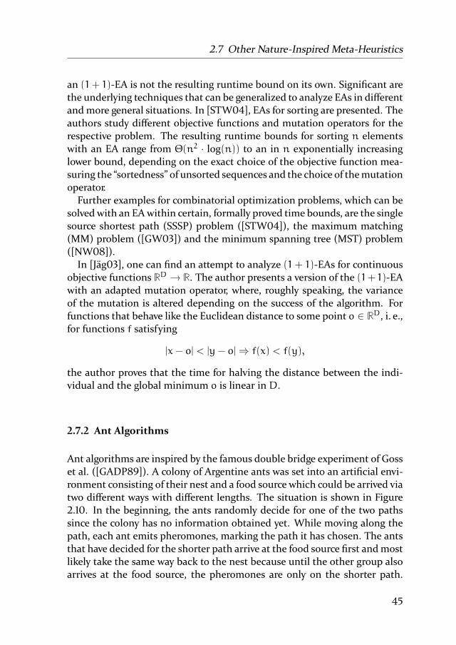
2.7 Other Nature-Inspired Meta-Heuristics
an (1+ 1)-EA is not the resulting runtime bound on its own. Significant are
the underlying techniques that can be generalized to analyze EAs in different
andmore general situations. In [STW04], EAs for sorting are presented. The
authors study different objective functions and mutation operators for the
respective problem. The resulting runtime bounds for sorting n elements
with an EA range from Θ(n2 · log(n)) to an in n exponentially increasing
lower bound, depending on the exact choice of the objective function mea-
suring the “sortedness” of unsorted sequences and the choice of themutation
operator.
Further examples for combinatorial optimization problems, which can be
solved with an EAwithin certain, formally proved time bounds, are the single
source shortest path (SSSP) problem ([STW04]), the maximum matching
(MM) problem ([GW03]) and the minimum spanning tree (MST) problem
([NW08]).
In [Jäg03], one can find an attempt to analyze (1+ 1)-EAs for continuousobjective functions RD → R. The author presents a version of the (1+ 1)-EAwith an adapted mutation operator, where, roughly speaking, the variance
of the mutation is altered depending on the success of the algorithm. For
functions that behave like the Euclidean distance to some point o ∈ RD, i. e.,for functions f satisfying
|x− o| < |y− o|⇒ f(x) < f(y),
the author proves that the time for halving the distance between the indi-
vidual and the global minimum o is linear in D.
2.7.2 Ant Algorithms
Ant algorithms are inspired by the famous double bridge experiment of Goss
et al. ([GADP89]). A colony of Argentine ants was set into an artificial envi-
ronment consisting of their nest and a food source which could be arrived via
two different ways with different lengths. The situation is shown in Figure
2.10. In the beginning, the ants randomly decide for one of the two paths
since the colony has no information obtained yet. While moving along the
path, each ant emits pheromones, marking the path it has chosen. The ants
that have decided for the shorter path arrive at the food source first andmost
likely take the same way back to the nest because until the other group also
arrives at the food source, the pheromones are only on the shorter path.
45
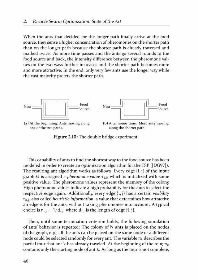
2. Particle Swarm Optimization: State of the Art
When the ants that decided for the longer path finally arrive at the food
source, they sense a higher concentration of pheromones on the shorter path
than on the longer path because the shorter path is already traversed and
marked twice. As more time passes and the ants go several rounds to the
food source and back, the intensity difference between the pheromone val-
ues on the two ways further increases and the shorter path becomes more
and more attractive. In the end, only very few ants use the longer way while
the vast majority prefers the shorter path.
NestFood
Source
(a) At the beginning: Ants moving along
one of the two paths.
NestFood
Source
(b) After some time: Most ants moving
along the shorter path.
Figure 2.10: The double bridge experiment.
This capability of ants to find the shortest way to the food source has been
modeled in order to create an optimization algorithm for the TSP ([DG97]).
The resulting ant algorithm works as follows. Every edge i, j of the input
graph G is assigned a pheromone value τi,j, which is initialized with some
positive value. The pheromone values represent the memory of the colony.
High pheromone values indicate a high probability for the ants to select the
respective edge again. Additionally, every edge i, j has a certain visibilityηi,j, also called heuristic information, a value that determines how attractive
an edge is for the ants, without taking pheromones into account. A typical
choice is ηi,j = 1/di,j, where di,j is the length of edge i, j.
Then, until some termination criterion holds, the following simulation
of ants’ behavior is repeated: The colony of N ants is placed on the nodes
of the graph, e. g., all the ants can be placed on the same node or a different
node could be selected randomly for every ant. The variable πk describes the
partial tour that ant k has already traveled. At the beginning of the tour, πkcontains only the starting node of ant k. As long as the tour is not complete,
46
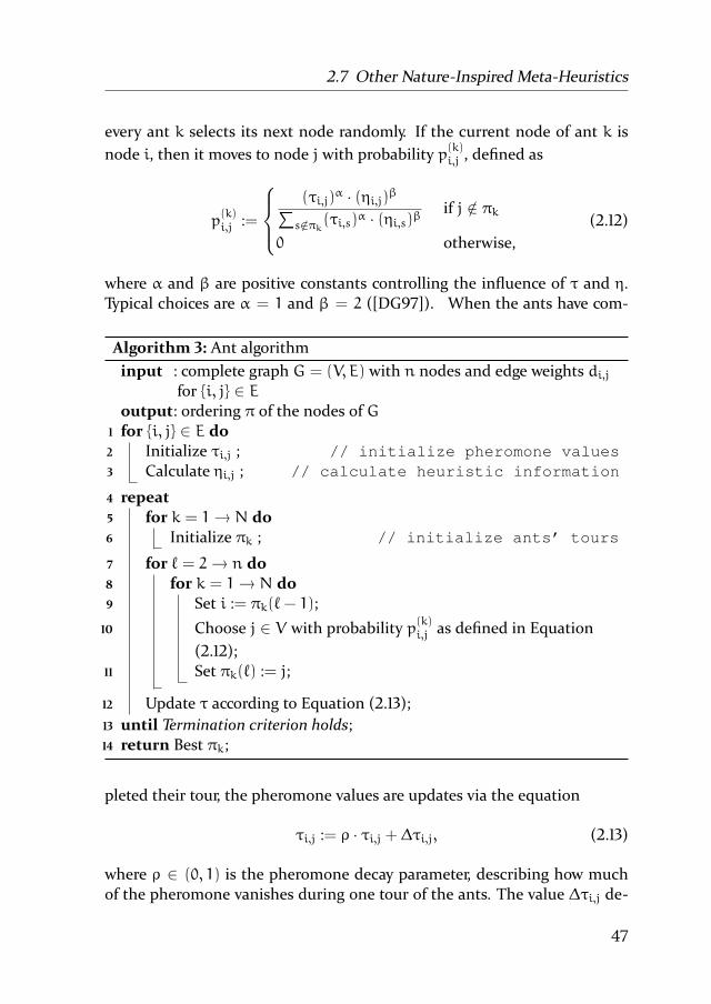
2.7 Other Nature-Inspired Meta-Heuristics
every ant k selects its next node randomly. If the current node of ant k is
node i, then it moves to node j with probability p(k)i,j , defined as
p(k)i,j :=
(τi,j)
α · (ηi,j)β∑s/∈πk(τi,s)
α · (ηi,s)βif j /∈ πk
0 otherwise,
(2.12)
where α and β are positive constants controlling the influence of τ and η.
Typical choices are α = 1 and β = 2 ([DG97]). When the ants have com-
Algorithm 3: Ant algorithminput : complete graph G = (V, E) with n nodes and edge weights di,j
for i, j ∈ Eoutput: ordering π of the nodes of G
1 for i, j ∈ E do2 Initialize τi,j ; // initialize pheromone values3 Calculate ηi,j ; // calculate heuristic information
4 repeat5 for k = 1→ N do6 Initialize πk ; // initialize ants’ tours
7 for ` = 2→ n do8 for k = 1→ N do9 Set i := πk(`− 1);
10 Choose j ∈ V with probability p(k)i,j as defined in Equation
(2.12);
11 Set πk(`) := j;
12 Update τ according to Equation (2.13);
13 until Termination criterion holds;14 return Best πk;
pleted their tour, the pheromone values are updates via the equation
τi,j := ρ · τi,j + ∆τi,j, (2.13)
where ρ ∈ (0, 1) is the pheromone decay parameter, describing how much
of the pheromone vanishes during one tour of the ants. The value ∆τi,j de-
47

2. Particle Swarm Optimization: State of the Art
scribes, by how much the pheromone value of edge i, j is increased by ants
moving over it. One example for a concrete choice of ∆τi,j is ([DG97])
∆τi,j =
N∑k=1
∆τ(k)i,j
with
∆τ(k)i,j =
1/L(k) if edge i, j is traversed by ant k,
0 otherwise,
where L(k) is the length of ant k’s tour. When the termination criterion holds,
the algorithm is stopped and the best tour visited by any ant is returned.
An algorithmic overview over the ant algorithm can be found in Algo-
rithm 3. For an overview over variants of the ant algorithm for binary prob-
lems, including some theoretical runtime results, see [NSW09].
48

3. PSO as a Stochastic Process
The main goal of this chapter is to provide a reformulation of the classical
particle swarm optimization (PSO) algorithm under a mathematical point
of view by describing it as a real-valued stochastic process. Additionally, wediscuss previous results in the light of this newmodel and formally introduce
drift theory as a mathematical tool for obtaining runtime results.
In the first section, we briefly recall some mathematical basics of proba-
bility theory, with strong emphasize on the situation of the standard contin-
uous black box optimization problem and differences to the discrete, com-
binatorial situation.
In the second section, we recall a strong negative result in the area of com-
binatorial optimization, namely the No Free Lunch (NFL) Theorem. The
statement of the NFL Theorem is, roughly speaking, that on average over
all possible combinatorial optimization problems, any two algorithms have
the same performance. In particular, that means that without at least some
knowledge about the objective function inside the black box, no method is
better than just randomly guessing search points. However, it turns out that
this result does not hold in the continuous setting.
In the third section, we introduce drift theory, an important tool for ob-
taining runtime results about evolutionary algorithms solving combinato-
rial optimization problems, which we adapt to the specific situation of PSO.
Roughly speaking, if some process is on expectation decreasing by a certain
amount, drift theory allows for bounds on the expected time until the pro-
cess hits, e. g., the value 0. Sincemost drift theorems from the literaturemore
or less implicitly rely on the combinatorial structure of the search space, we
prove a new drift theorem, which is explicitly designed to handle the contin-
uous case.
Finally, we provide the model of the PSO algorithm in terms of the intro-
duced mathematical concepts. In the light of this new formulation follows
a discussion of some of the theoretical results already mentioned in Section
2.6 of Chapter 2. In particular, we revisit the negative results saying that the
49

3. PSO as a Stochastic Process
expected time for optimization via PSO is infinite, andwe point out why they
are not in contradiction with the positive results of this thesis.
3.1 Basics of Probability Theory
In this section, we briefly recall some essential basics of probability theory,
we highlight some subtleties and we point out the crucial differences be-
tween the discrete and the continuous situation. The concepts and terms
introduced here can be found, e. g., in [Kle06] or [Bau96], usually in a much
more general way than stated here.
3.1.1 Probability Space, Random Variables, Stochastic Processes andConditional Expectation
Typically, a random experiment has some setΩ of possible outcomes, the so-
called sample space. The cardinality and the type of the elements of Ω are
not restricted. For instance, Ω = HEAD, TAIL, Ω = 1, 2, 3, 4, 5, 6, Ω = NandΩ = [0, 1], where [a, b] denotes the real interval from a to b, are possible.If Ω is at most countable, it is said to be discrete. If Ω is uncountable, it is
called continuous.IfΩ is discrete, the “probability” is usually defined by assigning a probabil-
ity value to every single outcome. However, in a typical continuous situation,
every single element of Ω has probability 0. So, instead of defining proba-
bility as a function Ω → [0, 1], the probability is defined as a function that
assigns a value to sets of outcomes, so-called events, rather than to the out-
comes itself. The set A ⊂ P(Ω), where P(Ω) denotes the power set of Ω,
defines which subsets of Ω are considered events. If Ω is discrete, usually
the choice A := P(Ω) is made. However, as we will see in Section 3.1.2, in
continuous situations this is in general not possible, i. e., there are subsets
A ⊂ Ω that do not have a well-defined probability.
The set A includes Ω and ∅, i. e., the case that none of the outcomes ac-
tually occurs and the case that any of the outcomes occurs are both events.
Additionally, for an event A ∈ A, the case that A does not happen, that
means the setΩ\A, is also an event and therefore included inA. Finally, for
50

3.1 Basics of Probability Theory
any countable number of events Ai ∈ A, the case that at least one of the Aihappens, i. e., the set
⋃iAi, is also considered an event. With thementioned
properties, A is called a sigma-field or sigma-algebra.The function P : A→ [0, 1] is called probability measure or for short prob-
ability, if it assigns 1 to Ω, i. e., the event that any of the outcome occurs
has probability 1, and if additionally P is countably additive, i. e., if for every
countable and mutual disjoint set of events Ai, the union of all the Ai has
probability P(⋃∞i=1Ai) =
∑∞i=1 P(Ai). Altogether, we have motivated the fol-
lowing definition of a probability space, consisting of the ground setΩ, the
sigma-field A ⊂ P(Ω) overΩ and the probability measure P : A→ [0, 1].
Definition 3.1 (Probability Space). A probability space is a triple (Ω,A,P),where
• Ω, the sample space, is an arbitrary, non-empty set,
• A ⊂ P(Ω), the set of events, is a sigma-field overΩ, i. e.,
– ∅ ∈ A,– A ∈ A⇒ Ω \A ∈ A,– A1, A2, . . . ∈ A⇒ ⋃∞
i=1Ai ∈ A,
• P, the probability measure, is a function A→ [0, 1], such that
– P(Ω) = 1,
– P is sigma additive, i. e., for every sequence A1, A2, . . . ∈ A of
mutually disjoint events, P(⋃∞i=1Ai) =
∑∞i=1 P(Ai)
The elements ofA are calledmeasurable with respect toA,A-measurable orP-measurable. If P only satisfies the weaker condition “P(A) ≥ 0 for every
A ∈ A” instead of “P(A) ∈ [0, 1] for every A ∈ A and P(Ω) = 1”, then P is
called a measure and (Ω,A,P) a measure space. If P(A) = 1 for some event
A, we say that A holds almost surely. If P(A) = 0, then A is called a null setwith respect to P or a P-null set.
A very important example for a sigma-field over RD is the so-called Borelalgebra B(RD), which is defined as the smallest sigma-field containing every
open subset O ⊂ RD, i. e., B(RD) is the intersection of all sigma-fields con-
taining every open subsetO ∈ R. Similarly, B(×Dd=1[ad, bd]) with ad, bd ∈ R
andad < bd for everyd = 1, . . . , D denotes the smallest sigma-field contain-
ing every open subset of the hyperrectangle×Dd=1[ad, bd]. More precisely:
B( D
×d=1
[ad, bd])=B ∩
D
×d=1
[ad, bd]∣∣ B ∈ B(RD).
51

3. PSO as a Stochastic Process
To complete the measure space over RD, the Lebesgue measure LD is defined
to serve as the uniform measure, i. e., it is defined as the unique measure
over RD that satisfies
LD( D
×d=1
[ad, bd])=
D∏d=1
(bd − ad)
for every a1, . . . , aD, b1, . . . , bD ∈ R with ad ≤ bd for every d = 1, . . . , D,
i. e., that assigns to every hyperrectangle the product of its lengthsmultiplied
over all dimensions. The proof of existence and uniqueness of LD can be
found in, e. g., [Kle06] or [Bau96]. Note that L1 restricted to [0, 1] is the
uniform probability distribution over [0, 1] and, more general, 1/(b− a) · L1restricted to [a, b] is the uniform probability distribution over [a, b].
The probability space ([0, 1]D,B([0, 1]D),LD) is suitable to model a ran-
dom experiment in which D values are uniformly and independently cho-
sen from the interval [0, 1], i. e., the well-known function “rand()” is called
D times. However, in the classical PSO, it is not a priori clear how often the
function “rand()” is called. Therefore, it is necessary to construct a probabil-
ity space overΩ = [0, 1]∞, the space of all sequences (ωi)i∈N withωi ∈ [0, 1]for every t ∈ N, which allows drawing an infinite number of values, chosen
uniformly and independently from the interval [0, 1]. The appropriate sigma-
field is the product sigma-field of infinitelymany instances of the sigma-field
B([0, 1]). Formally, a product sigma-field of sigma-fieldsAi with i ∈ I, whereI is some set of indices, is defined as follows.
Definition 3.2. Let I = (i1, i2, . . .) be a set of indices and let beΩi = [ai, bi]with ai < bi and Ai = B(Ωi) for every i ∈ I. The product sigma-field of the
Ai ⊗i∈IAi
is defined as the smallest sigma-field containing
Ωi1 × . . .×Ωik−1 × B×Ωik+1 × . . .∣∣ k ≤ |I|, B ∈ Aik.
Note that as a property of the Borel algebra, we have for finite I⊗i∈IB([ai, bi]) = B
(×i∈I
[ai, bi]).
52

3.1 Basics of Probability Theory
To complete the construction of the probability space for calling “rand()”
infinitely often, we need to define a probability measure
L∞ :⊗i∈N0
B([0, 1])→ [0, 1].
In order to construct L∞, we use a corollary to the Theorem of Ionescu-
Tulcea, which states that such a probability measure exists and is uniquely
defined.
Theorem 3.1 (Corollary to the Theorem of Ionescu-Tulcea, [Kle06]). For ev-ery i ∈ N, let (Ωi,Ai,Pi) be a probability space. Then, there is a uniquely
determined probability measure P on( ∞×i=0
Ωi,
∞⊗i=0
Ai),
such that
P
(A0 × . . .×An ×
∞×i=n+1
Ωi
)=
n∏i=0
Pi(Ai)
for every n ∈ N and every Ai ∈ Ai for i = 0, . . . , n.
In the following definition, we summarize the resulting probability space,
which we will use as the underlying probability space of the particle swarm.
Definition 3.3 (PSO probability space). The probability space R = (Ω,A,P)is defined via
• Ω := [0, 1]∞,
• A :=⊗
N B([0, 1]),
• P := L∞,
where [0, 1]∞ = (ω0,ω1, . . .) | ωi ∈ [0, 1] for every i ∈ N is the space of
all sequences with values in [0, 1],⊗
N B([0, 1]) is the product sigma-field of
countably many instances of B([0, 1]) and L∞ is obtained from Theorem 3.1
by setting (Ωi,Ai,Pi) = ([0, 1],B([0, 1]),L1).
In most cases, not the outcomes of a random experiment itself are inter-
esting, but some random observations which depend on the outcome. In
order to formally describe such random observations, we define the concept
of random variables.
53

3. PSO as a Stochastic Process
Definition 3.4 (Random Variable). Let (Ω,A,P) be a probability space. A
function X : Ω → RD is called a random variable, if X−1(B) ∈ A for ev-
ery B ∈ B(RD). In that case, we also say that X is measurable with re-spect to A, A-measurable or P-measurable. If X is a random variable, then
(RD,B(RD),PX−1) is a probability space and PX−1is called the distribution
of X. Additionally, σ(X) := X−1(B(RD)) is called the sigma-field generated byX.
Example 3.1 (Indicator Variable). The indicator variable of an event A ∈ Ais defined as
1A(ω) :=
1, ifω ∈ A,0, otherwise.
This is a random variable, because the preimage of a set B ∈ B(RD) under1A is
1−1A (B) =
∅, if 0, 1 /∈ B,A, if 0 /∈ B, 1 ∈ B,Ω \A, if 0 ∈ B, 1 /∈ B,Ω, if 0, 1 ∈ B.
The sets ∅ and Ω are included in A by definition and since A ∈ A, A also
contains the complementΩ \A.
In order to simplify notation, we let X ∈ B denote the event X−1(B) =ω ∈ Ω | X(ω) ∈ B for a random variable X and a B ∈ B(RD). Events likeX < a and X > b are defined analogously.
Instead of describing only a single random experiment, many randomized
systems evolve over time and perform some random state transition at every
time step t. In order to describe systems with such a time-dependent be-
havior, we use a sequence of random variables. That leads to the following
definition of a stochastic process.
Definition 3.5 (Stochastic Process, Filtration). A sequence of random vari-
ables X = (X0, X1, . . .) is called a stochastic process. A sequence of sigma-
fields F = (F0,F1, . . .) is called a filtration, if Ft ⊂ Ft+1 for every t ∈ N0.If Xt is measurable with respect to Ft, i. e., if for every t ∈ N0 and every
B ∈ B(RD) we have that X−1t (B) ∈ Ft, then X is called adapted to F.
Intuitively, we can think of Ft as the mathematical object that carries the
information about the stochastic process that is determined at time t and
54

3.1 Basics of Probability Theory
characterize events measurable with respect to Ft as the events from which
we know at time t if they happen or not. The following example illustrates
the use of knowledge about the past.
Example 3.2. Consider the probability space R fromDefinition 3.3. Forω =(ω0,ω1, . . .) ∈ [0, 1]∞ and let the stochastic process X = (X0, X1, . . .) be
defined as
Xt(ω) :=
t∑t ′=1
ωt ′ for every t ∈ N0.
The sigma-field Ft generated by Xt is the union of all sets of the form B ×[0, 1]∞ where B ∈ B([0, 1]t) and X is adapted to the sequence of sigma-fields
F = (Ft)t∈N. That means an element of Ft contains information about the
first t entries ofω, namely that (ω0, . . . ,ωt) ∈ B, but for t ′ > t, it only says
ωt ′ ∈ [0, 1].
In the following, we use information about the past to make predictions
about the future of a stochastic process, i. e., we want to take the perspective
of some time t andmake predictions (in terms of, e. g., the expectation value)
about the stochastic process at time s, where s > t, by taking the information
at time t into account. For formally stating such predictions, we define the
concepts of conditional probability and conditional expectation.The standard definitions of the conditional probability for some event A,
given some other event B as
P(A | B) :=P(A ∩ B)P(B)
(3.1)
and the conditional expectation of some random variable X given B as
E[X | B] :=E[X · 1B]P(B)
(3.2)
work fine for discrete situations, but for handling random variables over a
continuous search space, it is necessary to generalize these concepts. The
following example illustrates this.
Consider the stochastic process X = (X0, X1, . . .) from Example 3.2, where
X0 is uniformly distributed over [0, 1] and knowing the value x0 of X0, X1is uniformly distributed over [x0, x0 + 1]. Intuitively, the expectation of X1,
knowing that X0 = x0, should be x0 + 1/2, but the discrete definition of
conditional expectation (Equation (3.2)) cannot be applied because for ev-
ery x0, the “B”, i. e., the event X0 = x0, has probability 0. The solution of
55

3. PSO as a Stochastic Process
the stated issue is to define the conditional expectation itself as a random
variable. In the present example, we would write E[X1 | F0] = X0 + 1/2, arandom variable measurable with respect to F0. Formally, the definition of
the conditional expectation is generalized in the following way.
Definition 3.6 (Conditional Expectation). For a probability space (Ω,A,P),let F ⊂ A be a sigma-field and X a random variable. Then E[X | F ] denotesa random variable that fulfills the following two conditions.
• E[X | F ] is measurable with respect to F ,
• E[X1A] = E[E[X | F ]1A] for every A ∈ F .
The random variable E[X | F ] is called the conditional expectation of X givenF . Additionally, for an event B ∈ A, the conditional probability of B given Fis defined as
P(B | F) := E[1B | F ].
We can easily verify that in the previous example, indeed E[X1 | F0] =X0 + 1/2 holds.
Example 3.3. Consider the stochastic process X and the filtration F as de-
fined in Example 3.2. The candidate for the conditioned expectation E[X1 |F0] of X1 given F0 is Y := X0+ 1/2 = ω0+ 1/2. Since Y depends only onω0,
it is measurable with respect to F0. For every A ∈ F0, i. e., every A ⊂ [0, 1]∞of the form B× [0, 1]∞ with B ∈ B([0, 1]), we have
E[X11A] − E[Y1A] = E[(X1 − Y)1A]
=
∫A
X1(ω) − Y(ω) dP(ω)
=
∫B×[0,1]∞ X1(ω) − Y(ω) dP(ω)
=
∫B×[0,1]
(ω0 +ω1) − (ω0 + 1/2) d(ω0,ω1)
=
∫B×[0,1]
ω1 − 1/2 d(ω0,ω1)
= P(B) ·∫[0,1]
ω1 − 1/2 d(ω1) = 0.
That means that for every A ⊂ [0, 1]∞, E[X11A] = E[Y1A], which verifies the
second condition of Definition 3.6, so Y = E[X1 | F1] actually holds.
56

3.1 Basics of Probability Theory
As it is proved in, e. g., [Kle06] and [Bau96], the conditional expectation
exists and is uniquely determined up to null sets, i. e., the probability that
two randomvariableswhich both fulfill the conditions ofDefinition 3.6 differ
is 0. We will use the conditional expectation to formally model the drift ofa stochastic process, i. e., we formalize a statement like “on expectation, the
process X decreases by at least ε in every time step” as
∀t ∈ N0 : E[Xt+1 | Ft] ≤ Xt − ε.
Sometimes, the notation is slightly abused to state that a certain property
of E[Xt+1 | Ft] only holds under some condition. In general, for a sigma-
fieldF ⊂ A, anA-measurable random variable X, anF-measurable random
variables Y and an event C ∈ F , we write
E[X | F , C] ≤ Y :⇔ 1C · E[X | F ] ≤ 1C · Y.
This can be read as “if C occurs, then E[X | F ] ≤ Y.” Note that C ∈ F means
that the information provided by F is already sufficient to determine if C
occurs, i. e., if the actual outcomeω ∈ Ω is included inC. E. g., the statement
“on expectation, the process X decreases by at least ε in every time step as
long as X is positive” can be expressed as
∀t ∈ N : E[Xt+1 | Ft, Xt > 0] ≤ Xt − ε.
An important structural property of stochastic processes is the so-called
Markov property, which describes a process without a memory of its past. A
stochastic process has the Markov property, if predictions about its future,
taking information about its past and its present state into account are the
equal to the predictions using only the information about the current state.
The following definition provides a formal description of this property.
Definition 3.7 (Markov Property). A stochastic process (Xt)t∈N0 has the
Markov property, if
P(Xt ∈ A | Fs) = P(Xt ∈ A | σ(Xs))
for every A ∈ RD and every s, t ∈ N0 with s ≤ t. Here, σ(Xs) is the sigma-
field generated by Xs as defined in Definition 3.4.
57

3. PSO as a Stochastic Process
3.1.2 Measurability
The existence of non-measurable functions has important implications for
analyzing any randomized, continuous optimizationmethod. For anymean-
ingful statement about an optimization scenario,B(RD)-measurability of the
objective function is aminimum requirement. To illustrate this, we construct
an example for a non-measurable function, namely the indicator function
1V of a set V ⊂ [0, 1] that is itself not measurable with respect to B(R),i. e., V 6∈ B(R). Since sets that are defined constructively are usually B(R)-measurable, e. g., any countable union of intervals is B(R)-measurable, the
construction of V is more complex. Consider the equivalence relation R on
[0, 1]× [0, 1], defined via
r ≈R s :⇔ r− s ∈ Q,
i. e., two real numbers r, s ∈ [0, 1] are considered equivalent, if their differ-
ence is rational. Then, the equivalence class of some r ∈ [0, 1] is
[r] = (r+ Q) ∩ [0, 1] := r+ q | q ∈ Q ∩ [0, 1].
Since Q is countable, every equivalence class contains a countable number
of elements and since the interval [0, 1] is uncountable, there are uncount-
ably many equivalence classes. The set V is defined as any set that contains
exactly one representative of every equivalence class. In the literature (e. g.,
[Kle06]), V is calledVitali Set. Since every real number r ∈ [0, 1] is equivalentto some element v ∈ V and since −1 ≤ r− v ≤ 1, it follows that
[0, 1] ⊂ V + Q ∩ [−1, 1] := v+ q | v ∈ V, q ∈ Q ∩ [−1, 1].
Additionally, since V ⊂ [0, 1], we have that
V + Q ∩ [−1, 1] ∈ [−1, 2].
Defining
Vq := V + q = v+ q | v ∈ V
for someq ∈ Q∩[−1, 1] as the setV , shifted byq, we can rewriteV+Q∩[−1, 1]as
V + Q ∩ [−1, 1] =⋃
q∈Q∩[−1,1]
Vq.
58

3.1 Basics of Probability Theory
Altogether, it follows that
[0, 1] ⊂⋃
q∈Q∩[−1,1]
Vq ⊂ [−1, 2], (3.3)
i. e., the countable union of all the Vq covers [0, 1] and is contained in [−1, 2].Furthermore, it is easy to see that the Vq are disjoint. Assume, for con-
tradiction, that v ∈ Vq1 ∩ Vq2 for some q1 6= q2. Then, we would have
V 3 v − q1 6= v − q2 ∈ V , which contradics the definition of V since
v− q1 ≈R v− q2.Keeping these properties in mind, the hypothetical optimization problem
is defined as follows:
Maximize f(x) = 1V(x) over the search space S = [−1, 2].
A search heuristic that maximizes f is successful as soon as it finds a point
v ∈ V . Assuming that the first step consists of uniformly sampling a point of
the search space, the success probability would be the probability of V under
uniform distribution. Let P be the respective probability measure, defined
as P(A) := 1/3 · L(A ∩ [−1, 2]). Then, from (3.3), it follows that
1
3= P([0, 1]) ≤ P
( ⋃q∈Q∩[0,1]
Vq
)≤ 1.
Furthermore, the sigma-additivity of probability measures and the transla-
tion invariance of the uniform distribution imply
P
( ⋃q∈Q∩[0,1]
Vq
)=∑
q∈Q∩[0,1]
P(Vq) =∑
q∈Q∩[0,1]
P(V).
This results in
1
3≤
∑q∈Q∩[0,1]
P(V) ≤ 1,
a contradiction because either P(V) = 0, then∑q∈Q∩[0,1] P(V) = 0 < 1/3
or P(V) > 0, then∑q∈Q∩[0,1] P(V) = ∞ > 1. This illustrates that there is
no meaningful way to define the probability of the constructed set V under
uniform distribution and therefore the success probability for optimizing f
is undefined from the first step on. Similar investigations show that all other
interesting characteristics like the expected optimization time are undefined
59

3. PSO as a Stochastic Process
as well. So, measurability of the objective function is a minimum require-
ment for making any valid statements about the quality of some random-
ized optimization method. Although the non-measurable example function
looks very artificial, in the following section we will point out that measur-
able functions have some structural properties that have significant conse-
quences for the continuous black box optimization problem.
3.2 (No) Free Lunch and Lebesgue’s Differentiation Theorem
A fundamental result in the area of combinatorial black box optimization
is the so-called No Free Lunch Theorem ([WM97]). Basically, it states that
in presence of a finite search space, no deterministic or randomized search
method is superior to any other with respect to the number of objective func-
tion evaluations. Therefore, in absence of problem specific knowledge, there
is no algorithm that works better than, e. g., randomly sampling points of the
search space. The formal statement and the proof can be found in ([WM97]).
The key idea of the proof is to assume that the objective function f is chosen
randomly from the space of “all” possible objective functions, before the op-
timization algorithm is applied. Then, for any permutation π of the search
space, f π is also a valid objective function. Therefore, with the k pairs of
search points and their function values (x1, f(x1)), . . . , (xk, f(xk)), the distri-bution of the function value f(x), given (x1, f(x1)), . . . , (xk, f(xk)), with some
search point x not already sampled, does not depend on the particular choice
of x. In other words: For every subset A of the image of f and every x, x with
x 6= x and x, x /∈ x1, . . . , xk, we have P(f(x) ∈ A) = P(f(x) ∈ A). Therefore,the information about the values of f at the search points x1, . . . , xk does not
imply any preference on the remaining search points.
It is remarkable that in the continuous case, i. e., when the search space is
uncountable, the situation is completely different ([AT10]). That is because
the set of BD-measurable functions has a structural property that is known
as Lebesgue’s Differentiation Theorem.
Theorem 3.2 (Lebesgue’s Differentiation Theorem). For z ∈ RD and r > 0,
Br(z) denotes the ball with center z and radius r. Let f be a BD-measurable
60

3.3 Drift Theory
function, such that
∫RD f(x)dx exists. Then for almost every x ∈ RD, the
limit
lim
r→0 1
|Br(z)|
∫Br(z)
|f(x) − f(z)|dx
exists and is equal to 0.
As a stochastic interpretation, we can think about the random experiment
that uniformly samples points with a distance of at most r from some fixed
point z. Then the theorem says that for almost every point z, as r is de-
creased towards 0, the value obtained will approach f(z) almost surely. This
means that f behaves very similar to a continuous function. As pointed out
in [AT10], this is already enough structural information to prove that the No
Free Lunch Theorem can not be generalized to the continuous case. There-
fore, there is indeed hope to find optimization methods that are superior to
the blind search method of randomly sampling search points.
3.3 Drift Theory
Drift Theory has proved its value as an important tool for analyzing evolu-
tionary algorithms for combinatorial optimization problems. Examples for
successful application are, among others, the optimization time of a (1+ 1)-EA for optimizing linear functions over 0, 1D ([HY04, Jäg08, DJW12]), cal-
culatingminimum spanning trees ([NW07,DG10]), solving the single source
shortest path problem ([BBD+09, DJ10, DG10]) and finding a Eulerian cycle
([DG10]). Originally, He and Yao ([HY01]) introduced drift theory to the field
of evolutionary algorithms by usingmathematical results of Hajek ([Haj82]).
The goal of drift analysis is to provide sufficient conditions to bound the time
τ := inf t ≥ 0∣∣ Xt ≤ 0 until some stochastic process X reaches 0. This is
straight-forward if the process is non-increasing and has a bounded min-
imum decrease, but if the process decreases only on expectation, while it
might with some positive probability increase as well, things get more com-
plicated.
61

3. PSO as a Stochastic Process
3.3.1 Classical Drift Theory
Consider a stochastic processX = (Xt)t∈N, adapted to a filtrationF = (Ft)t∈N,
such that one of the following drift conditions holds.
E[Xt+1 − Xt∣∣ Xt > 0] ≤ −δ, (3.4)
or
E[Xt+1 − Xt∣∣ Ft, Xt > 0] ≤ −δ (3.5)
for some δ > 0. Condition (3.4) states that under the condition that Xt > 0,
the process will decrease by δ, i. e., this is the expectation we have at time 0.
Stronger than this, Condition (3.5) states that for every state of the stochas-
tic process X at time t, the uniform bound of −δ holds for the conditional
expectation of Xt+1 − Xt. Although Condition (3.5) is formally a stronger
assumption than Condition (3.4), it is usually easier to handle and to verify.
If such a drift condition holds, i. e., if we can expect the process X to de-
crease by at least δ at each time step, one would intuitively assume that after
at most E[X0]/δ iterations, the process reaches 0, i. e., the expectation E[τ] ofthe time τ := inf t ∈ N | Xt ≤ 0 for Xt becoming ≤ 0 should be bounded
from above by E[X0]/δ. However, in general there is a difference between the
time T := inf t ∈ N | E[Xt] ≤ 0, the deterministic time when the expecta-
tion of the stochastic process reaches 0, and the expectation of the random
time τ. The following example illustrates this.
Example 3.4. Consider the following stochastic process.
X0 :=
2, with probability
12 ,
4, with probability12 ,
Xt+1 :=
2, if X0 = 2,
Xt − 2, otherwise.
If X0 = 2, which happens with probability 1/2, then the process will stay 2
forever and τ is infinite. Otherwise, X0 = 2 and Xt = 4 − 2 · t. In that case,
τ = 2. Altogether, τ has an infinite expectation. On the other hand, we have
that E[Xt] = 3− t, i. e., T = 3.
Typical drift theorems say that under the drift condition (Condition (3.4)
or Condition (3.5)) and some additional assumptions, such pathological cases
can be avoided and the bound E[τ] ≤ E[X0]/δ actually holds. Additionally,
by replacing “≤” with “≥” in Condition (3.4) and Condition (3.5), a lower
62

3.3 Drift Theory
bound on the drift is achieved and drift theory leads to a lower bound of
E[X0]/δ for τ.Depending on the nature of the algorithm which is analyzed and on the
underlying stochastic process, sometimes the drift conditions are expressed
multiplicatively, i. e., instead of expecting an absolute decrease of X during
every iteration, we assume that X decreases on expectation by a constant
factor 1− δ ([DJW12]). Then, the drift condition has the form
E[Xt+1 − Xt∣∣ Ft, Xt > 1] ≤ −δ · Xt (3.6)
and drift theory yields, again under some additional assumptions, the upper
bound E[τ∣∣ Ft] ≤ ln(X0)/δ. Note that in case of a multiplicative drift theo-
rem, in contrast to the additive case, the modified drift condition, where “≤”is replaced by “≥”, does not imply any lower bound on E[τ].
There are many slightly different drift theorems in the literature, varying
in the assumptions which aremade in addition to the drift condition. Typical
additional assumptions are chosen from the following collection:
• Xt has a finite image ([HY04, DJW12]),
• Xt /∈ (0, 1) for every t ∈ N ([DG10]),
• X0 ≤ b for some constant b ∈ R ([HY01]),
• Xt ≥ 0 for every t ∈ N ([HY01, DG10]),
• |Xt+1 −Xt| ≤ c for a constant c ∈ R+and every t ∈ N ([Jäg07, Jäg08]),
In a discrete scenario, all of these assumptions are trivial or at least very
easy to fulfill. However, for calculating runtime bounds for PSO, such as-
sumptions become crucial. In the following section, we provide a new variant
of the drift theorem, suitable for the continuous situation and in particular
for obtaining runtime results about the optimization time of PSO.
3.3.2 Drift Theory for Continuous Search Spaces
When analyzing the drift of some stochastic process, themost important dif-
ference between the discrete and the continuous situation is that only in the
continuous scenario, the state of the algorithm can be outside but arbitrary
close to the region considered optimal. If a process X = (Xt)t∈N, adapted
63

3. PSO as a Stochastic Process
to a filtration F = (Ft)t∈N, is continuous but non-negative, a condition like
Condition (3.5) from the previous section is unsatisfiable. That is because
for non-negative image of the Xt, we have
E[Xt+1 − Xt∣∣ Ft, Xt > 0] ≥ E[−Xt
∣∣ Ft, Xt > 0] = −Xt,
which can be arbitrary close to 0 for small values of Xt. Therefore, we cannot
expect Condition (3.5) to hold with any constant δ. To solve this issue, we
develop a modified drift theorem, which allows for X to have negative val-
ues. If the process X serves as a measure for some optimization algorithm,
that means that the elements of the optimized region do not all have the
same value 0 as in the discrete setting. Instead, they can have any value ≤ 0.However, as the following example illustrates, the drift condition alone does
not imply any upper bound on the expected time for X to hit 0.
Example 3.5. For the constants x0 > 0, δ > 0, we consider the following
stochastic process X = (X0, X1, . . .).
X0 := x0, Xt :=
Xt−1, w. p. 1− 1/3t
Xt−1 − 3t · δ, w. p. 1/3t,
for t > 0.
This process fulfilles Condition 3.5:
E[Xt+1 − Xt∣∣ Ft, Xt > 0] = (1− 1/3t) · 0+ 1/3t · (−3t · δ) = −δ.
However, to actually arrive at a value ≤ 0, the second case of the definition
of Xt must happen at least once. Therefore, for the probability for X to reach
a value ≤ 0, we have
P(∃t : Xt ≤ 0) ≤∞∑t=1
1
3t=1
2,
i. e., the time τ until X passes 0 is with probability at least 1/2 infinite and
has therefore infinite expectation.
The reason, why in Example 3.5 no meaningful bound on the first hitting
time of X hitting R≤0 could be achieved, is that the expected drift results in a
process that with very little probability decreases dramatically, while it stays
constant with overwhelming probability. Therefore, additionally to the drift
condition, we need an assumption for our drift theorem that forbids such
pathological cases.
64
3.3 Drift Theory
As a possible solution, we ask for a drift≤ −δ even for themodified process
that decreases at most by a constant ∆, i. e., we want maxXt+1 − Xt,−∆ toyield an expected drift ≤ −δ. As it turns out, this modification allows us
for an upper bound only slightly larger than with the prerequisite of a non-
negative process.
The following result is a modified version of the additive drift theorem
presented in [HY01].
Theorem 3.3 (Additive Drift Theorem). Let ∆ > δ > 0 be some constants.
Let X = (Xt)t∈N be a stochastic process adapted to a filtration F0 ⊂ F1 ⊂. . . ⊂ F , such that
E[maxXt+1 − Xt,−∆∣∣ Ft, Xt > 0] ≤ −δ, (3.7)
Let τ := mint ≥ 0∣∣ Xt ≤ 0 be the first index when Xt passes 0. Then
E[τ∣∣ F0] ≤ 1X0>0 · (X0 + ∆)/δ.
For the proof of Theorem 3.3, we want to apply the Lemma of Fatou, a
convergence result from the area of stochastic processes.
Lemma 3.1 (of Fatou ([Kle06, Bau96])). Let Y = (Y0, Y1, . . .) be a stochasticprocess, such that Yt ≥ 0 almost surely for every t ∈ N. Then,
lim inft→∞ E[Yt] ≥ E[lim inf
t→∞ Yt].
Proof (of Theorem 3.3). Since X0 ≤ 0 implies τ = 0, we can without loss of
generality assume that X0 > 0 and therefore τ ≥ 1 almost surely. We then
define the stochastic process Y = (Y0, Y1, . . .) via
Yt := maxXmint,τ + ∆, 0+ δ ·mint, τ.
65

3. PSO as a Stochastic Process
Note that every Yt is non-negative and measurable with respect to Ft. Addi-tionally, we have
E[Yt+1∣∣ Ft] = E
[1τ>t · Yt+1
∣∣ Ft]+ E
[1τ≤t · Yt+1
∣∣ Ft]= E
[1τ>t · (maxXt+1 + ∆, 0+ δ · (t+ 1))
∣∣ Ft]+ 1τ≤t · (maxXτ + ∆, 0+ δ · τ)
≤ 1τ>t ·E[maxXt+1 − Xt,−∆+ Xt + ∆+ δ·(t+ 1)
∣∣ Ft]+ 1τ≤t · Yt
(3.7)
≤ 1τ>t · (−δ+ Xt + ∆+ δ · (t+ 1)) + 1τ≤t · Yt
= 1τ>t · (maxXt + ∆, 0+ δ · t) + 1τ≤t · Yt
= 1τ>t · Yt + 1τ≤t · Yt = Yt,
i. e., Yt ≥ E[Yt+1∣∣ Ft]. By induction and from X0 + ∆ = Y0, it follows that
X0 + ∆ ≥ E[Yt∣∣ F0] for every t and therefore
X0 + ∆ ≥ lim inf
k→∞ E[Yt∣∣ F0] (∗)≥ E[lim inf
t→∞ Yt∣∣ F0]
= E[lim inft→∞ (maxX
mint,τ, 0)︸ ︷︷ ︸≥0
+δ · τ∣∣ F0]
≥ δ · E[τ∣∣ F0].
The inequality (∗) is obtained from Lemma 3.1. This finishes the proof.
Originally, the authors of [HY01] used Lebesgue’s Theorem of Dominated
Convergence ([Kle06, Bau96]) instead of Lemma 3.1. Therefore, they needed
the additional assumption that every Xt is bounded from above by a con-
stant. While this is obviously true if Xt has a finite image, this requirement
cannot be fulfilled in the analysis of PSO.
Next, the drift theorem is transferred from an additive situation to a mul-
tiplicative one. The following theorem is basically the multiplicative drift
theorem from [DJW12] with just slightly changed preconditions.
Theorem 3.4 (Multiplicative Drift Theorem). Let X = (Xt)t∈N be a strictly
positive stochastic process adapted to a filtration F0 ⊂ F1 ⊂ . . . ⊂ F , suchthat
E[maxXt+1/Xt, e−∆
∣∣ Ft, Xt > 1] ≤ 1− δ (3.8)
66

3.3 Drift Theory
for some δ ∈ (0, 1) and ∆ > δ. Let τ := mint ≥ 0∣∣ Xt ≤ 1 be the first index
when Xt passes 1. Then
E[τ∣∣ F0] ≤ 1X0>1 · (ln(X0) + ∆)/δ.
Proof. The proof is essentially the same as in [DJW12]. The idea is to use the
additive drift theorem on the stochastic process (Zt)t∈N, where Zt := ln(Xt).Then (3.8) translates to
1Zt>0 · E[maxZt+1 − Zt,−∆∣∣ Ft]
= 1Xt>1 · E[ln(maxXt+1/Xt, e−∆)
∣∣ Ft](∗)≤ 1Xt>1 · ln(E[maxXt+1/Xt, e
−∆∣∣ Ft])
≤ 1Xt>1 · ln(1− δ) ≤ 1Zt>0 · (−δ)
For (∗), we apply Jensen’s inequality. Since τ = mint ≥ 0∣∣ Xt ≤ 1 =
mint ≥ 0∣∣ Zt ≤ 0, Theorem 3.3 finishes the proof.
For the runtime analysis, we need a more general version of the multi-
plicative drift theorem. Sometimes, the stochastic process needs more than
just one step to reduce its value by a constant factor, e. g., depending on the
current configuration, the process might yield Xt+1 > Xt, but for every sit-
uation, we have that Xt+2 < Xt · (1 − δ). So, instead of the drift condition
(3.8), only the weaker drift condition
E[maxXt+tmax/Xt, e
−∆∣∣ Ft, Xt > 1] ≤ 1− δ
holds for some tmax ∈ N. In that case, we would expect τ to increase by a
factor of tmax.
In a more general situation, the point in time σ when Xt decreases on
expectation by at least a factor of 1− δ, i. e., the value σ(t) for which
E[maxXσ(t)/Xt, e−∆
∣∣ Ft, Xt > 1] ≤ 1− δholds, might depend on the exact configuration at time t, e. g., wemight have
that either Xt+2 < Xt · (1 − δ) or Xt+3 < Xt · (1 − δ), and which alternative
is true is known at time t but is not known a priori. However, as long as σ(t)is uniformly bounded by tmax, we can still expect that τ increases by at most
a factor of tmax. The following generalized version of the multiplicative drift
theorem formally confirms this statement.
67

3. PSO as a Stochastic Process
Theorem 3.5 (Multiplicative Drift Theorem with Variable Time Steps). Let
X = (Xt)t∈N be a strictly positive stochastic process adapted to a filtration
F0 ⊂ F1 ⊂ . . . ⊂ F , and let for every t ∈ N σ(t) be a Ft-measurable, N-
valued random variable with t < σ(t) ≤ t+ tmax almost surely for a constant
tmax ∈ N, such that
E[maxXσ(t)/Xt, e−∆
∣∣ Ft, Xt > 1] ≤ 1− δ (3.9)
for some δ ∈ (0, 1) and ∆ > δ. Let τ := mint ≥ 0∣∣ Xt ≤ 1 be the first index
when Xt passes 1. Then
E[τ∣∣ F0] ≤ tmax · 1X0>1 · (ln(X0) + ∆)/δ.
Proof. To simplify notation, we write σk for σ(k)(0). For every k ∈ N, we
define Xk := Xσk and Fσk := A ∈ F∣∣ A ∩ σk ≤ t ∈ Ft. Then, Xk is
Fσk-measurable and since
E[maxXk+1/Xk, e−∆
∣∣ Fσk ] = E[maxXσk+1/Xσk , e−∆
∣∣ Fσk ]= E
[ ∞∑t=0
1σk=t ·maxXσk+1/Xσk , e−∆
∣∣ Fσk]
=
∞∑t=0
1σk=t · E[maxXσk+1/Xσk , e
−∆∣∣ Fσk]
=
∞∑t=0
1σk=t · E[maxXσ(t)/Xt, e
−∆∣∣ Ft] ,
Xk > 1 implies
E[maxXk+1/Xk, e−∆
∣∣ Fσk ]=
∞∑t=0
1σk=t · E[maxXσ(t)/Xt, e
−∆∣∣ Ft]
≤∞∑t=0
1σk=t · (1− δ) = 1− δ,
i. e.,
1Xk>1· E[maxXk+1/Xk, e
−∆∣∣ Fσk ] ≤ 1Xk>1
· (1− δ).
Theorem 3.4 yields for τ = mink ≥ 0∣∣ Xk ≤ 1 the expected bound of
E[τ∣∣ Fσ0 ] ≤ (ln(X0) + ∆)/δ = (ln(X0) + ∆)/δ+ 1.
68

3.3 Drift Theory
Since τ ≤ τ · tmax, we have that
E[τ∣∣ F0] ≤ tmax · E[τ
∣∣ F0] = tmax · E[τ∣∣ Fσ0 ] ≤ tmax · (ln(X0) + ∆)/δ.
That finishes the proof.
Although the result of our multiplicative drift theorem for continuous
search spaces is a bound, only an additive constant larger than in the dis-
crete case, the drift condition on maxXt+1/Xt, e−∆ is kind of impractical
and technical harder to verify than a drift condition on Xt+1/Xt. Note that
the construction of Example 3.5, showing that in an additive situation a drift
condition on Xt+1 − Xt is insufficient, has no pendant in the multiplicative
situation, where the process X is allowed to take only positive values. Indeed,
we can provide a multiplicative drift theorem, that is not a rewritten version
of an additive drift theorem, but is proved directly.
Theorem 3.6 (Multiplicative Drift Theorem II). LetX = (Xt)t∈N be a strictly
positive stochastic process adapted to a filtration F0 ⊂ F1 ⊂ . . . ⊂ F , suchthat
E[Xt+1∣∣ Ft, Xt > 1] ≤ (1− δ) · Xt (3.10)
for some δ ∈ (0, 1). Let τ := mint ≥ 0∣∣ Xt ≤ 1 be the first index when Xt
passes 1. Then
E[τ∣∣ F0] ≤ 1X0>1 · (ln(X0) + 2)/δ.
Proof. First, we define the stochastic process Y = (Y0, Y1, . . .) via
Y0 := X0, Yt+1 :=
Xt+1, if τ > t,
Yt · (1− δ), if τ ≤ t.
That means Yt is equal to Xt until time τ. Afterwards, Y decreases determin-
istically by a factor of 1− δ in every iteration. In particular, this implies that
both processes reach a value≤ 1 at the same time, i. e., τ = mint ≥ 0∣∣ Yt ≤
1, and Yt is Ft-measurable and fulfilles the stronger drift condition
E[Yt∣∣ Ft] ≤ (1− δ) · Yt.
By induction, it follows that
E[Yt+1∣∣ F0] ≤ (1− δ)t · Y0 = (1− δ)t · X0.
Therefore, we have for the first hitting time τ:
P(τ > t∣∣ F0) = P(Yt > 1
∣∣ F0) ≤ (1− δ)t · X0,
69

3. PSO as a Stochastic Process
where the inequality comes from Markov’s inequality. It follows that
E[τ∣∣ F0] =
∞∑t=0
P(τ > t∣∣ F0)
≤b− log1−δ X0c∑
t=0
1+
∞∑t=d− log1−δ X0e
(1− δ)t · X0
≤ −ln(X0)
ln(1− δ)+ 1+
∞∑s=0
(1− δ)s
≤ ln(X0)
δ+ 1+
1
δ≤ ln(X0) + 2
δ.
Of course, the same generalization, that allowed us to prove Theorem 3.5
from Theorem 3.4, can be applied here in order to obtain a version of The-
orem 3.6, that allows for the drift to happen after a bounded random time.
The result is the following theorem, which we will use for the analsis of PSO.
Theorem3.7 (MultiplicativeDrift Theoremwith Variable Time Steps II). LetX = (Xt)t∈N be a strictly positive stochastic process adapted to a filtration
F0 ⊂ F1 ⊂ . . . ⊂ F , and let for every t ∈ N σ(t) be a Ft-measurable, N-
valued random variable with t < σ(t) ≤ t+ tmax almost surely for a constant
tmax ∈ N, such that
E[Xσ(t)∣∣ Ft, Xt > 1] ≤ (1− δ) · Xt (3.11)
for some δ ∈ (0, 1). Let τ := mint ≥ 0∣∣ Xt ≤ 1 be the first index when Xt
passes 1. Then
E[τ∣∣ F0] ≤ 1X0>1 · tmax · (ln(X0) + 2)/δ.
Proof. The proof is completely analog to the proof of Theorem 3.5.
The reason for the increased bounds for τ in all the drift theorems pre-
sented in this section, compared to “E[τ∣∣ F0] ≤ ln(X0)/δ” in the discrete
case, is that over a discrete search space, we can use an argument like “if
Xt < 2, then Xt ≤ 1”, i. e., as soon as the difference between the process
and the optimum is smaller than the distance between two neighbors of the
discrete space, the optimum is already reached. In the continuous situation,
such an argument cannot hold and the remaining distance between “2” and
“1” is not for free like in the discrete case, but needs to be paid with an addi-
tional constant number of steps.
70

3.4 The PSO Model
3.4 The PSOModel
With the prerequisites from the previous sections, we can state PSO as a
stochastic process. The following definition describes the positions, veloci-
ties and attractors of the classical PSO algorithm as random variables over
the probability space R, as defined in Definition 3.3.
Definition 3.8 (Classical PSO Process). A swarm S of N particles moves
through the D-dimensional search space RD. Let f : RD → R be the ob-
jective function. For S, over the probability space R from Definition 3.3 the
stochastic process
S = (St)t∈N0 = ((Xt, Vt, Lt, Gt))t∈N0 = ((X0, V0, L0, G0), (X1, V1, L1, G1), . . .)
is defined, consisting of
• Xt = (Xn,dt )1≤n≤N,1≤d≤D (d-th coordinate of the position of particle n
after step t),
• Vt = (Vn,dt )1≤n≤N,1≤d≤D (d-th coordinate of the velocity of particle n
after step t),
• Lt = (Ln,dt )1≤n≤N,1≤d≤D (d-th coordinate of the local attractor of par-ticle n after step t),
• Gt = (Gn,dt )1≤n≤N,1≤d≤D, (d-th coordinate of the global attractor be-fore step t+ 1 of particle n).
To simplify notation, Xnt denotes the vector (Xn,1t , ..., Xn,Dt ) (analogously, Vnt ,Lnt , G
nt ) and X
dt the vector (X1,dt , ..., X
N,dt ) (analogously, Vdt , L
dt , G
dt ), when-
ever the context allows a clear distinction. Furthermore, Gn,dt denotes the
d-th coordinate of the global attractor after the t-th step of particle n, i. e.,
Gn,dt = Gn+1,dt if n < N, and GN,dt = G1,dt+1. With a given distribution for
(X0, V0) and the values G10 := argmin1≤n≤Nf(Xn0 ) and L0 := X0, St+1 =
(Xt+1, Vt+1, Lt+1, Gt+1) is determined by the following recursive equations,
the movement equations:
• Vn,dt+1 = χ · Vn,dt + c1 · rn,dt+1 · (Ln,dt − Xn,dt ) + c2 · sn,dt+1 · (Gn,dt − Xn,dt ) fort ≥ 0,
• Xn,dt+1 = Xn,dt + Vn,dt+1 for t ≥ 0,
• Lnt+1 = argminXnt+1,Lnt f,
71

3. PSO as a Stochastic Process
• Gn+1t = argminLnt+1,Gnt f for t ≥ 0, 1 ≤ n ≤ N− 1,
• G1t+1 = argminLNt+1,GNt f for t ≥ 0.
In case of a tie when applying argmin, similar to the PSO version in [OH07],
the new value prevails, i. e., whenever a particle finds a search point with
value equal to the one of its local attractor, this point becomes the new local
attractor. If additionally the value is equal to the one of the global attrac-
tor, this one is also updated. Here, χ, c1 and c2 are some positive constants
called the fixed parameters of S, and rn,dt , sn,dt are uniformly distributed over
[0, 1] and all independent, i. e., each of the rn,dt and sn,dt is identified with a
differentωi from Definition 3.3.
If after the t-th step the process is stopped, the solution found by S so
far is GNt . This process describes exactly the PSO variant of Algorithm 1 in
Section 2.2. The major part of this thesis will study the limit of the sequence
(GNt )t∈N as t tends to∞.
Definition 3.8 describes the common movement equations with the same
two specifications as stated in the algorithmic description of PSO (Section
2.2, Algorithm 1): If a particle visits a point with the same objective value as
its current local attractor or the current global attractor, then the respective
attractor is updated to the new point. As pointed out in [OH07], this is cru-
cial in the case of objective functions that are constant on some area with a
positive Lebesgue measure. As the second specification, the global attractor
is updated after every step of a single particle, not only after every iteration
of the whole swarm. Another common variant of PSO, sometimes known
as parallel PSO, only updates the global attractor after every iteration of the
whole swarm. However, due to the choice we make here, the information
shared between the particles is as recent as possible.
From Definition 3.8, it follows that (St)t∈N has the Markov property, i. e.,
the distribution of St+t0 given all the previous values (S0, . . . , St0) is the same
as the distribution of St+t0 given only St0 . This is clear because St+1 is for-
mulated in terms of St and some random variables rn,dt+1 and sn,dt+1 which are
independent of the past of S. Another interesting property of this stochastic
process that follows immediately from the movement equations is the fol-
lowing:
Observation 3.1. Let S be a swarm and ((Xt, Vt, Lt, Gt))t∈N0 its correspond-
ing stochastic process. Let Lk denote the k-dimensional Lebesgue measure,
L[Y] the distribution of a random variable Y and “” (just in this observa-
tion) absolute continuity between two distributions. Assuming L[(X0, V0)]
72

3.4 The PSO Model
L2·N·D, it follows L[Xt] LN·D for every t ≥ 0. If Xnt 6= GNt for every n,
then for every t ′ > t, L[Xt ′∣∣ St] LN·D almost surely.
This observation follows from the structure of the movement equations,
i. e., the entries of Xt are weighted sums of the entries of X0, which by as-
sumption has probability 0 to hit any fixed Lebesgue null set, and values that
are chosen uniformly and independently from certain intervals. If Xnt 6= GNtfor every n, then for every t ′ > t, the entries of Xt ′ are sums of constants
depending on St and a non-empty sum of values, chosen uniformly and in-
dependently from certain intervals.
For the coming analysis, we introduce the notion of a potential of a swarm.
Basically, the potential is an extension of the physical interpretation of the
particle swarm model. If the particles move faster and get farther away from
their global attractor, the potential increases. If the swarm converges, the
potential tends towards 0. At the different stages of the analysis, different
measures for the potential will be useful. The following definition describes
the two most frequently used formulations for a measure of the potential.
Definition 3.9 (Potential). For a > 0, we define the measure Φn,dt for the
potential of swarm S in dimension d right before the t-th step of particle n
as
Φn,dt :=
√√√√ n−1∑n ′=1
(a|Vn
′,dt |+|Gn,dt−1 − X
n ′,dt |
)+
N∑n ′=n
(a|Vn
′,dt−1 |+|Gn,dt−1 − X
n ′,dt−1 |
).
To simplify notation, Φn,dt describes the same potential measure in dimen-
sion d after the t-th step of particle n, i. e.,
Φn,dt :=
√√√√ n∑n ′=1
(a|Vn
′,dt |+|Gn,dt−1 − X
n ′,dt |
)+
N∑n ′=n+1
(a|Vn
′,dt−1 |+|Gn,dt−1 − X
n ′,dt−1 |
).
As another measure for the potential, we define the potential of particle n
in dimension d right after the t’th step of the last particle N as
Yn,dt :=√
|Vn,dt |+√|G1,dt − Xn,dt |.
While Φ only measures the potential of the whole swarm, Ynt is able to
measure the potential of a single particle. Note that this are not the only
possible choices for a meaningful measure of the swarm’s potential. How-
ever, for technical reasons explained later, this particular potential measures,
73

3. PSO as a Stochastic Process
including the additional parameter a for later use and the occurring square
roots, are necessary. General tendencies towards 0 or∞ are invariant under
the different measures. In particular, Φ1t+1 and∑Nn=1 Y
n,dt are equivalent in
the sense that they deviate by at most a constant factor.
3.5 Discussion of Previous Results
In the light of this new model for PSO, which we will use for the rest of this
thesis, some of the previous positive and negative results, relevant for the
results of this thesis, need to be revisited in more detail.
3.5.1 Negative Results
Since the goal of this thesis is to prove rigorous results about the convergence
of the PSO process and the runtime, a discussion of the various negative re-
sults, which appear to be in contradiction to the results of this thesis, is nec-
essary. A very popular negative result comes from considering the following
situation (e. g., [vdBE10, Wit09, PE03, BM14]).
X1t = L1t = . . . = X
Nt = LNt = G1t = z,
V1t = . . . = VNt = 0,
for some z ∈ RD, i. e., all the attractors and particles’ positions are located at
the same point z ∈ RD and every velocity is 0. From Definition 3.8, it follows
that
X1t ′ = L1t ′ = . . . = X
Nt ′ = L
Nt ′ = G
1t ′ = z,
V1t ′ = . . . = VNt ′ = 0,
for every t ′ ≥ t. That means that the particles will stay at z forever, no
matter how good or bad f(z) is. Therefore, so the claim frequently found in
the literature, providing any positive result about the quality of the returned
solution or even about the runtime is impossible.
However, if the positions and velocities of the initial population are dis-
tributed in some natural way, e. g., uniformly at random over K, Observa-
tion 3.1 states that the swarm has similar restrictions as a process consisting
74
3.5 Discussion of Previous Results
only of variables that are sampled u. a. r. in the sense that events with proba-
bility 0 in the latter case also have probability 0 in the first case. Since RD is
not enumerable, under uniform sampling no point in RD is drawnmore than
once and therefore the particle swarm also does not visit any pointmore than
once. This implies that this well-studied equilibrium when every particle is
at the global attractor and has velocity 0 is a state that the process may con-
verge to but that can never be reached. In other words: The probability for
the above mentioned equilibrium to be reached within any finite time t is 0
and therefore, this pathological event has no effect on the expected runtime.
Another, yet more refined negative result can be found in [LW11]. Here, the
authors consider the very simple, 1-dimensional objective function SPHERE,
defined as
SPHERE(x) = x2,
and construct an event that indeed has a positive probability to occur and
fromwhich the particles will with probability 1 not reach a certain neighbor-
hood of the unique local and therefore global optimum at 0. To be precise,
the authors of [LW11] proof the following theorem.
Theorem 3.8 (Proposition 1 in [LW11]). The first hitting time τε with respect
to ε is defined as the first time when the algorithm obtains a search point
x ∈ RD, such that |f(x)| < ε, i. e., the first time when the algorithm finds a
search point with a value atmost εworse than the optimum. Then there is an
ε > 0, such that the classical PSO with inertia factor χ < 1 and one particle
has infinite expected first hitting timewith respect to ε on the 1-dimensional
SPHERE.
In the following, we briefly outline the proof idea. If (without loss of gen-
erality) the particle is initialized at a negative position and has a positive ve-
locity, then both attractors will be equal to its current position until it passes
75

3. PSO as a Stochastic Process
the optimum at 0. This implies that until the optimum is passed, we have
V1,1t = χt · V1,10 and therefore
X1,1t = X1,10 +
t−1∑s=0
·V1,1s
= X1,10 + V1,10 ·t−1∑s=0
χs
≤ X1,10 + V1,10 ·∞∑s=0
χs
≤ X1,10 + V1,10 ·1
1− χ.
Since χ < 1, 1/(1 − χ) is a bounded value, there is a positive probability for
the event X1,10 + V1,10 ·11−χ < −
√ε, if ε > 0 is sufficiently small. In [LW11],
the authors call such an event a bad initialization event. Consequently, thereis a positive probability for the particle to never hit any value closer than√ε to the optimum at 0, which implies that for the considered objective
function SPHERE, no point with a function value of at most ε will be visited.
Note that the condition χ < 1 is not a true restriction since this is one of
the convergence conditions identified in [JLY07b, JLY07a]. Therefore, the
authors of [LW11] have proved that the classical PSO with only one particle
is not an effective optimizer.
On the other hand, for generalizing the same idea to the case of more than
one particle, further restrictions to the parameters χ, c1 and c2 are necessary.
The result for the case of two particles is as follows.
Theorem 3.9 (Theorem 1 in [LW11]). Consider the classical PSO with two
particles on the 1-dimensional SPHERE. If χ < 1, 1 < c2 < 2, V1,10 , V
2,10 ≤ 0,
κ < 1 where
κ :=c22 − 2 · c2 + 2+ 2 · χ · c2
4 · c2
+
√(c22 − 2 · c2 + 2+ 2 · χ · c2) · (c22 + 6 · c2 + 2+ 2 · χ · c2)
4 · c2,
and
X1,10 , X2,10 > 2 · ε+ 2 · c2 ·
(|X2,10 − X1,10 |+ |V1,10 |+ |V2,10 |
(1− χ) · (1− κ)
)76

3.5 Discussion of Previous Results
all hold together, then the expected first hitting time with respect to ε is
infinite.
The proof idea is the same as in Theorem 3.8, i. e., under the stated as-
sumptions, the swarmwill with positive probability never pass the optimum.
However, the crucial prerequisite of Theorem 3.9 is κ < 1. We can easily ver-
ify that this is typically violated by parameters common in the literature.
Table 3.1 provides an overview over some parameter choices famous in the
literature and the resulting values for κ.
Table 3.1: Famous parameter choices and the resulting values for κ
χ c1 c2 κ
0.72984 1.49617 1.49617 1.78756
0.72984 2.04355 0.94879 1.91517
0.6 1.7 1.7 1.66267
Therefore, the result from [LW11] does not contradict a runtime analysis
of the classical PSO with appropriately chosen parameters.
3.5.2 Convergence Analysis
The convergence analysis from [JLY07b, JLY07a] provides results about the
expectation and the variance of the particles’ positions under the assump-
tion that the local and global attractor are constant. Although in this thesis
we do not make this assumption, we will use an altered version of their proof
in Chapter 4, therefore we present the main results and the proof here. With
constant local attractors Lnt =: Ln and a constant global attractor Gnt =: G,we can write movement equations can as
Vn,dt+1 = χ · Vn,dt + c1 · rn,dt+1 · (Ln,d − Xn,dt ) + c2 · sn,dt+1 · (Gd − Xn,dt ), (3.12)
Xn,dt+1 = Xn,dt + Vn,dt+1. (3.13)
Since the processes ((Xn1,d1t , Vn1,d1t ))t∈N and ((Xn2,d2t , Vn2,d2t ))t∈N are inde-
pendent of each other if n1 6= n2 or d1 6= d2, it is sufficient to study just one
of these processes, or equivalently formulated, to study the case of only one
particle in a 1-dimensional search space. Therefore, the upper indices n and
d will be omitted for the rest of this section.
77

3. PSO as a Stochastic Process
Theorem 3.10 (Theorem 1 in [JLY07b]). Given χ, c1, c2 ≥ 0, if and only if
0 ≤ χ < 1 and 0 < c1 + c2 < 4 · (1 + χ), iterative process (E[Xt])t∈N is
guaranteed to converge to
µ :=c1 · L+ c2 ·Gc1 + c2
.
Proof. The proof from [JLY07b] will be briefly recalled. Rewriting Equation
(3.13) as Vt+1 = Xt+1−Xt, we can in Equation (3.12) replace Vt+1 by Xt+1−Xtand Vt by Xt − Xt−1. After collecting terms, we obtain
Xt+1 = (1+χ−c1 ·rt+1−c2 ·st+1) ·Xt−χXt−1+c1 ·rt+1 ·L+c2 ·st+1 ·G (3.14)
and consequently
E[Xt+1] = (1+ χ−c1 + c22
) · E[Xt] − χ · E[Xt−1] +c1 · L+ c2 ·G
2. (3.15)
Equation (3.15) is a linear recursion of second order for the sequence (E[Xt])t∈N
with characteristic polynomial
λ2 −
(1+ χ−
c1 + c22
)· λ+ χ.
The sequence (E[Xt])t∈N converges if and only if the eigenvalues
λ1, λ2 =1
2·
(1+ χ− c1 + c22
)±
√(1+ χ−
c1 + c22
)2− 4 · χ
both have an absolute value strictly less than 1. As straightforward calcula-
tions show, this is the case for 0 ≤ χ < 1 and 0 < c1 + c2 < 4 · (1 + χ). Theactual limit µ of the sequence is then found by solving the equation
µ = (1+ χ− c1 · rt+1 − c2 · st+1) · µ− χ · µ+ c1 · rt+1 · L+ c2 · st+1 ·G,
which is obtained from Equation (3.14) by replacing Xt+1, Xt and Xt−1 with
µ.
Similarly, the authors of [JLY07b, JLY07a] calculated conditions for the se-
quence (Var[Xt])t∈N to converge. Their result is
78

3.5 Discussion of Previous Results
Theorem 3.11 (Theorem 3 in [JLY07b]). Given χ, c2, c2 ≥ 0, if and only if
0 ≤ χ < 1, c1 + c2 > 0 and f > 0 where
f := 1−
((1+ χ−
c1 + c22
)2+1
12· (c21 + c22) − χ
)· (1− χ) − χ3
are all satisfied together, iterative process (Var[Xt])t∈N is guaranteed to con-
verge to
1
6·(c1 · c2c1 + c2
)2· (G− L)2 · 1+ χ
f.
As a consequence, if the parameter restrictions from Theorem 3.10 and
Theorem 3.11 hold and G = L, i. e., the global attractor is equal to the local
attractor, then both theorems together imply that the positions of all par-
ticles converge towards µ almost surely because the expectation E[Xt] con-verges towards µ and the variance Var[Xt] converges towards 0. Additionally,we can derive a result about the convergence speed. Since the solution of the
recursive Equation 3.15 has the form
E[Xt] = d1 · λt1 + d2 · λt2 + µ
for some constants d1 and d2, the expected difference between Xt and µ de-
creases exponentially in t.
Although this result relies on constant local and global attractors, a prereq-
uisite that in general we cannot assume, the calculations can be generalized
to the case of attractors that are not a priori constant, but have a bounded
and small area, e. g., a neighborhood of the global optimum, which they do
not leave. We will introduce, prove and use this generalization in the second
part of Chapter 4.
79


4. Convergence of 1-dimensional PSO
After invalidating the different negative results, stating that classical particle
swarm optimization (PSO) was unable to converge towards a local optimum,
this chapter contains the main theoretical results of this thesis, namely pos-
itive results about the quality and the convergence speed of the unmodified
PSO algorithm for certain classes of 1-dimensional objective functions. In
the first part of this chapter, we present a proof of the convergence of PSO
towards a local optimum, showing that under comparatively mild assump-
tions about the objective function, the particles find at least a local optimum.
In the second part, we apply the drift theory methods introduced in Chapter
3 in order to prove that for an also very large class of objective functions, PSO
converges towards the optimum with linear convergence speed, i. e., the dis-
tance between the global attractor and the actual optimum is halved within
a constant number of iterations.
Note that we prove all the results in this chapter completely rigorously, that
means we only make certain restrictions on the set of admissible objective
functions, while we do not modify the PSO algorithm. Instead, we fully take
its stochastic nature into account andmake no unproved assumptions about
the behavior of the particles.
4.1 Particle Swarm Optimization Almost Surely Finds Local Optima
Finding a global optimum of a given objective function f is the ultimate goal
of any optimization method. However, in a continuous domain, achieving
this goal is hardly possible because two functions with different global op-
tima can be very similar andmight differ only on an arbitrary small subset of
the search space. For an example of two such functions f1 and f2, see Figure
4.1.
81

4. Convergence of 1-dimensional PSO
-10 -8 -6 -4 -2 0 2 4 6 8 10-20
0
20
40
60
80
100
(a)Objective function f1(x).
-10 -8 -6 -4 -2 0 2 4 6 8 10-20
0
20
40
60
80
100
(b)Objective function f2(x).
Figure 4.1: Two possible objective functions f1 and f2. The area on which
both are equal is large but the global optima are far away from
each other.
Therefore, in order to handle such functions, an algorithm needs to enter
every arbitrary small subcube of the search space. This request is in con-
tradiction with convergence because convergence of the algorithm implies
that after some finite time only points within a certain neighborhood are
queried. Therefore, for the rest of the search space, only a finite number of
function evaluations is performed, which is insufficient to hit every arbitrary
small subcube. Therefore, the actual goal of our analysis performed here is
to prove that the classical PSO algorithm finds at least a local optimum.
PSO is designed to handle any objective function, but for the rest of this
section, only objective functions from the setF defined below are considered.
Definition 4.1. Let f : RD → R be a function. f ∈ F if and only if
(i) there is a compact set K ⊂ RD with positive Lebesgue measure, such
that P(Xn0 ∈ K) = 1 for every n and
x ∈ RD
∣∣ f(x) ≤ supK f(the
island) is bounded;
(ii) f is continuous.
Restriction (i) states that there is a compact set K such that for all x ∈ K,the set of all search points y at least as good as x, i. e., all y with f(y) ≤ f(x),is a bounded set. For illustration of this restriction, see Figure 4.2.
Since the particles are initialized insideK and since f(Gnt ) is non-increasingin t, (i) ensures that the possible area for the global attractor is limited if the
positions of all particles are initialized inside of K (being on any point of the
82

4.1 Particle Swarm Optimization Almost Surely Finds Local Optima
Initialization of particles' positions
Possible area of global attractor
Figure 4.2: Valid objective functions.
island is better than being in the sea). If for example lim|x|→∞ f(x) =∞ or if
f has compact support and is negative onK, (i) is already satisfied. E. g., com-
mon benchmark functions like the function SPHERE or the function ROSEN-
BROCK ([Ros60]) are in F. On functions that violate (i), the swarm might
move forever because either they do not necessarily have a local optimum
like f(x) = x or they have an optimum, but improvements can be made arbi-
trary far away from it, like, e. g. in the case of the function f(x) = x2/(x4+1),where x = 0 is the only local and the global optimum, but if the particles
are far away from 0, they tend to further increase the distance because f con-
verges to 0 as |x| approaches∞. Figure 4.3 gives an illustration of this situ-
ation. Under such circumstances, convergence cannot be expected and it is
necessary to restrict the function class in order to avoid this. However, (ii)
might be the only true restriction. Note that every continuous function is
in particular measurable, therefore restricting the set of admissible objec-
tive functions according to Definition 4.1 avoids the problem mentioned in
Section 3.1.2.
83

4. Convergence of 1-dimensional PSO
-20 -15 -10 -5 0 5 10 15 200
0.5
1
1.5
2
2.5
3
3.5
4particle
local attractor
global attractor
(a) After initialization
-20 -15 -10 -5 0 5 10 15 200
0.5
1
1.5
2
2.5
3
3.5
4particle
local attractor
global attractor
(b) After iteration 1
-50 -40 -30 -20 -10 0 10 200
0.5
1
1.5
2
2.5
3
3.5
4particle
local attractor
global attractor
(c) After iteration 2
Figure 4.3: Particles processing f(x) = x2/(x4 + 1) and moving away from
the only local optimum because of the misleading landscape.
4.1.1 Proof of Convergence Towards a Local Optimum
For proving the convergence of a particle swarm, we first define the exact
sense of “swarm convergence.”
Definition 4.2 (Swarm Convergence). Swarm S converges if there almost
surely is a point z such that the following two conditions hold:
1. limt→∞ Vt = 0 (the movement of the particles tends to zero),
2. limt→∞ Xnt = z for eachn ∈ 1, . . . ,N (every particlemoves towards z).
A consequence of the above conditions is that limt→∞Gnt = z almost
surely and limt→∞ Lnt = z almost surely for every n ∈ 1, . . . ,N. Although
the convergence analysis in the literature ([JLY07a]) usually makes the as-
sumption that at least the global attractor is constant forever, a prerequisite
84

4.1 Particle Swarm Optimization Almost Surely Finds Local Optima
that because of Observation 3.1 cannot be assumed here, the generalization
of the convergence proof from [JLY07a], showing that their results still hold
under the weaker assumption of only the convergence of the attractors, is
straight-forward.
Our goal is to prove more, namely, that under the stated assumptions
about f the swarm is able to find a local minimum. Here, the notion of
the potential of a swarm comes into play. Roughly speaking, as long as the
swarm has potential high enough to overcome the distance to at least one
local minimum, the probability to find it within a few steps is positive. A
problem occurs when the value of the potential is too low for the swarm to
overcome the distance to the next optimum by only a small number of steps.
In other words, if f is monotonically decreasing in some direction and on an
area that is large in comparison to the potential of the swarm, the particles
must be able to “run down the hill,” i. e., they must be able to surpass every
distance as long as f decreases. The following definition formally describes
the situation of a swarm while it is “running down the hill.”
Definition 4.3 (Running Particle Swarm). Let d0 ≤ D be an arbitrary di-
mension. The swarm S is called positively running in direction d0 at time t,
if the following properties hold for every n ∈ 1, . . . ,N:
• Gn,d0t = max1≤i≤NXi,d0t ′ for t ′ = t+ 1 if i < n and t ′ = t otherwise,
• sign(Ln,d0t − Xn,d0t ) ≥ 0,
• Vnt ≥ 0 for every n.
Analogously, the swarm is called negatively running in direction d0 at time t,
if
• Gn,d0t = min1≤i≤NXi,d0t ′ for t ′ = t+ 1 if i < n and t ′ = t otherwise,
• sign(Ln,d0t − Xn,d0t ) ≤ 0,
• Vnt ≤ 0 for every n.
Intuitively, one may think of running as the behavior a swarm shows when
itmoves through an area that ismonotone in one dimensiond0, while chang-
es in any other dimension are insignificant. Therefore, in case of a positively
running swarm, the larger the d0’th entry of a position or attractor is, the
better is its function value. Note that if the state of being running is main-
tained long enough, all particles will eventually overcome their own local
85

4. Convergence of 1-dimensional PSO
attractors. From that point on, as long as the swarm stays running, the local
attractors of the particles are identical to their current positions. An example
of a running swarm is presented in Figure 4.4.
particle
local attractor
global attractor
Figure 4.4: A particle swarm in the state called “running”.
Example 4.1. Consider a 1-dimensional particle swarm and the objective
function f(x) = −x. Assume that the velocities of the particles are all posi-
tive. Then the swarm is positively running in direction 1 forever. It is obvious
that the position with the greatest x-value leads to the smallest value of f(x)and therefore becomes the global attractor. It remains to prove that the ve-
locity of every particle stays positive. Given the old velocity Vn,1t , the new
velocity Vn,1t+1 is a positive linear combination of the three components Vn,1t ,
Gn,1t − Xn,1t and Ln,1t − Xn,1t . The value for Vn,1t is positive by assumption,
Gn,1t −Xn,1t and Ln,1t −Xn,1t are non-negative sinceGn,1t ≥ Ln,1t ≥ Xn,1t . There-
fore, the velocity stays positive and the swarm will stay positively running
forever. In that situation, a good behavior would be increasing (or at least
non-decreasing) Φ.
The negative results of [LW11], recalled in Section 3.5.1 of the previous
chapter, can be read in the following way: “Under certain conditions on the
parameters χ, c1 and c2, a running swarm loses potential and therefore con-
verges.”
Informally speaking, if a swarm S has a too smallΦ to make it to the next
local minimum, it is necessary that Φ increases after S has become run-
ning, and so Φ enables the swarm to overcome every distance. The follow-
ing lemma is the central technical observation of this section and makes a
statement about how to choose the parameters to make sure that a running
swarm has an exponentially increasing potential.
86

4.1 Particle Swarm Optimization Almost Surely Finds Local Optima
Lemma 4.1 (Running to Infinity Lemma). For certain parameters N, χ, c1and c2, there is a q, 0 < q < 1, such that the event that the swarm S is posi-
tively (negatively, resp.) running in direction d0 and has a positive potential
Φ implies that on expectation the reciprocal of the potentialΦ decreases by
at least a factor of q, in terms:
E
[Φ1,d0t
Φ1,d0t+1
∣∣ Φ1,d0t > 0∧ S positively running ,Ft−1
]< q. (4.1)
Therefore, if S stays positively running forever, then Vn,d0t +Xn,d0t (−Vn,d0t −
Xn,d0t , resp.) tends to∞ for every n almost surely and the swarm leaves every
bounded set B ⊂ RD almost surely.
Proof. To ease up notation, the upper index d0 is omitted for the rest of this
proof. Without loss of generality, we can assume that the swarm is positively
running. Note that due to Observation 3.1, the case Φnt = 0 for some t and
some n has probability 0 and can therefore be neglected.
First, we need to bound the expression E
[Φ1t/Φ
1t+1
∣∣ Φ1t > 0∧ S positively
running,Ft−1]for the concrete choice of potential from Definition 3.9.
Values for N, χ, c1 and c2, for which this potential fulfills Equation (4.1)
for a q < 1 need to be determined. In other words, during one iteration of all
particles, the reciprocal of the potential should decrease on expectation by
at least a factor of q. By inserting the definition of Φ and applying the fact
that the swarm is positively running and therefore Xnt ≤ G1t and Vnt−1 ≥ 0 forevery n, we obtain:
Φ1tΦ1t+1
=
√√√√∑Nn ′=1
(a · |Vn ′
t−1|+ |G1t−1 − Xn ′t−1|)∑N
n ′=1
(a · |Vn ′
t |+ |G1t − Xn ′t |)
=
√√√√∑Nn ′=1
(a · Vn ′
t−1 +G1t−1 − X
n ′t−1
)∑Nn ′=1
(a · Vn ′
t +G1t − Xn ′t
)=
√√√√ ∑Nn ′=1
(a · Vn ′
t−1 +G1t−1 − X
n ′t−1
)∑Nn ′=1
(a · Vn ′
t +N · (Gn ′t−1 −G
n ′t−1) +G
1t−1 − X
n ′t
)=
√1∑N
n ′=1wn ′xn ′
≤N∑
n ′=1
wn ′ ·√xn ′ ,
87

4. Convergence of 1-dimensional PSO
where
wn ′ :=a · Vn ′
t−1 +G1t−1 − X
n ′t−1∑N
i=1
(a · V it−1 +G1t−1 − Xit−1
)and
xn ′ :=a · Vn ′
t−1 +G1t−1 − X
n ′t−1
a · Vn ′t +N · (Gn ′
t−1 −Gn ′t−1) +G
1t−1 − X
n ′t
.
The last inequality follows from the generalized weighted mean inequality
between the (−1)-mean and the (1/2)-mean with weights wn ′ . Note that
the wn ′ sum up to 1 and that they only depend on St−1, i. e., they are Ft−1-measurable. Therefore, it follows
E
[Φ1tΦ1t+1
∣∣ Ft−1]≤ E
[N∑
n ′=1
wn ′ ·√xn ′
∣∣ Ft−1]
=
N∑n ′=1
wn ′ · E[√xn ′
∣∣ Ft−1] ≤ max
n ′=1...NE
[√xn ′
∣∣ Ft−1]It remains to show, that E
[√xn ′
∣∣ Ft−1] ≤ q for every n ′ and a q < 1. By
applying the definition of xn ′ and the movement equations and replacing
the non-negative term c1 · rn′
t · (Ln′
t−1−Xn ′t−1) with 0 in the first “≤”, we obtain
xn ′ =a · Vn ′
t−1 +G1t−1 − X
n ′t−1
a · Vn ′t +N · (Gn ′
t−1 −Gn ′t−1) +G
1t−1 − X
n ′t
≤a · Vn ′
t−1 +G1t−1 − X
n ′t−1
a · (χ · Vn ′t−1 + c2 · sn
′t · (Gn
′t−1 − X
n ′t−1))+
· · ·+N ·max0, Xn′
t−1 + χ · Vn′
t−1 + c2 · sn′
t · (Gn′
t−1 − Xn ′t−1) −G
n ′t−1+
· · ·+G1t−1 − Xn′
t−1 − χ · Vn′
t−1 − c2 · sn′
t · (Gn′
t−1 − Xn ′t−1)
=a · Vn ′
t−1 +G1t−1 − X
n ′t−1
(a− 1) · (χ · Vn ′t−1 + c2 · sn
′t · (Gn
′t−1 − X
n ′t−1)) +G
1t−1 − X
n ′t−1+
· · ·+N ·max0, Xn′
t−1 + χ · Vn′
t−1 + c2 · sn′
t · (Gn′
t−1 − Xn ′t−1) −G
n ′t−1
88

4.1 Particle Swarm Optimization Almost Surely Finds Local Optima
There are two distinct cases. In the first case, the position of particle n ′
before its step is equal to the global attractor, in terms Gn′
t−1 = Xn′
t−1, which
in particular implies that G1t−1 = Xn′
t−1 since Xn ′t−1 ≤ G1t−1 ≤ Gn
′t−1. Then its
move is deterministic and its new position will be the new global attractor.
In this case, we obtain:
E
[√xn ′
∣∣ Ft−1] ≤√
a · Vn ′t−1
(a− 1) · χ · Vn ′t−1 +N · χ · Vn
′t−1
=
√a
(a− 1) · χ+N · χ,
which is less than q if and only if a < (N− 1) · χ·q21−χ·q2 .
The second case when G1t−1 > X1t−1 requires more exhaustive but still
straight-forward calculations. The expression
sup
v>0,g≥d>0
∫ 10
√av+ d
(a− 1)(χv+ c2sg) +Nmax0, χv+ c2sg− g+ dds
= sup
v ′>0,g ′>1
∫ 10
√av ′ + 1
(a− 1)(χv ′ + c2sg ′) +Nmax0, χv ′ + c2sg ′ − g ′+ 1ds
needs to be bounded.
The calculation of the integral can be done explicitly and finding the val-
ues for v ′ and g ′ maximizing it for given a, χ, c2 andN using standard tech-
niques from analysis is straight-forward. Obviously, the greater the number
of particles is, the smaller is the value of the integral, so we calculate themin-
imal number of necessary particles ensuring that the integral is less than 1
for three common parameter choices obtained from the literature. For the
choice of χ = 0.72984, c2 = 1.496172 recommended in [CK02, BK07], we
choose a := 2.3543 and obtain forN = 2 an upper bound of q ≤ 0.9812. Forthe choice χ = 0.72984 and c2 = 0.94879 ([CD01]), we require at leastN = 3particles and the choice of a := 5.1298 leads to q ≤ 0.9964. Finally, for thechoice χ = 0.6, c2 = 1.7 as proposed in ([Tre03]), for N = 3 and a := 2.5847we obtain a value of q ≤ 0.9693.
In Figure 4.5, we can see the borderlines between choices for c2 and χ that
satisfy the conditions of Lemma 4.1 and those that do not. We will refer to
the parameters that satisfy both Lemma 4.1 and the convergence require-
ments from Theorem 3.11 as “good” parameters. They are a counterpart to
89

4. Convergence of 1-dimensional PSO
0 0.1 0.2 0.3 0.4 0.5 0.6 0.7 0.8 0.9 10
1
2
3
4
5
6
7
Figure 4.5: Borders between the too low values for c2 and χ and the ones
large enough to satisfy the requirements in Lemma 4.1 for some
swarm sizes N.
the parameters satisfying the conditions of [LW11] from Section 3.5.1 in the
previous chapter, which can be seen as “bad” parameters that allow stagna-
tion on arbitrary search points with positive probability. However, there are
still parameters that satisfy neither the conditions from Section 3.5.1 nor the
conditions here, so they are neither good nor bad. From here on, we assume
that the parameters are good.
Lemma 4.1 says that, given the parameters are good, a swarm that moves
into the right direction can overcome every distance and increase its poten-
tial, no matter how small it was in the beginning. In other words: The equi-
librium, when all attractors and particles are on the same point and every
velocity is zero, is not stable because arbitrary small changes of an attractor,
a position or a velocity can be sufficient to lead the swarm far away from
this equilibrium, as long as there is a direction with decreasing value of the
objective function. This is already sufficient to prove the main result of this
section.
Theorem 4.1. If D = 1, then every accumulation point of the sequence of
global attractors G = (Gnt )n=1,...,N;t∈N is a local minimum of f almost surely.
Proof. Assume for contradiction, that there is an accumulation point z ∈ Rsuch that (w. l. o. g.) f is monotonically decreasing onBτ(z) = (z−τ, z+τ) forsome τ > 0. Since z is an accumulation point, for every ε > 0 G is inside the
90

4.1 Particle Swarm Optimization Almost Surely Finds Local Optima
ε-neighborhood Bε(z) = (z− ε, z+ ε) of z infinitely often. Figure 4.6 gives a
visualization of the described situation. Note that Gnt entering [z, z + τ] forany t and any n violates the assumption of z being an accumulation point.
That is because the global attractor does not accept worsenings, so for any ε
with ε < |z−Gnt |, Bε(z) will not be entered by the global attractor anymore.
Figure 4.6: Objective function f monotonic on Bτ(z), global attractor in ε-neighborhood of z
Now two cases need to be considered. The first case is that there is at least
a second accumulation point (that might even be a local optimum). This
second accumulation point must yield the same function value as z and can
therefore not be inside Bτ(z). Consequently, infinitely often, a particle has
a distance of at least τ between its local and its global attractor. From this
situation, the probability for hitting [z, z + τ] within the next few steps is
positive and the probability for never hitting [z, z + τ] would be 0. To prove
this, it is sufficient to outline a sequence thatmoves the particle into [z, z+τ].
Several different situations could occur: There are essentially three pos-
sible orders of the particle, its local attractor and z, depending on which of
this three points is between the other two. Furthermore, the velocity could
be close to 0 or large and it could point in two different directions. Since the
calculations showing that hitting [z, z+τ]has a positive probability fromeach
of the situations are straight-forward, we present them exemplary only. Con-
sider the case where z is located between the particles position Xnt and its lo-
cal attractor Lnt and has a velocityVnt with |Vnt | ≤ (c1·|Lnt −Xnt |−|z−Xnt |−τ)/χpointing away from Lnt . Then, any choice of rnt ∈ I with
I =
[|z− Xnt |+ τ/4− χ · |Vnt |
c1 · |Lnt − Xnt |,|z− Xnt |+ 3/4 · τ− χ · |Vnt |
c1 · |Lnt − Xnt |
]∩ [0, 1]
leads to Xnt+1 ∈ [z, z+ τ]. Since
|z− Xnt |+ τ/4− χ · |Vnt | ≤ |z− Xnt |+ τ/4 ≤ c1 · |Lnt − Xnt |− 3/4 · τ
91

4. Convergence of 1-dimensional PSO
and
|z− Xnt |+ 3/4 · τ− χ · |Vnt | ≥ c1 · |Lnt − Xnt |− τ/4,
we have |I| ≥ min1, τ4·c1·|Lnt −Xnt |
. If |Vnt | is larger than assumed above, we re-
quire at most two additional steps in order to decrease it sufficiently. Similar
calculations for all the other cases show that there is indeed always a positive
probability to hit [z, z+ τ] within a constant number of iterations. Addition-
ally, since |Lnt −Xnt | is stochastically bounded due to the choice of admissible
objective functions, the probability can not converge to 0. It follows that the
probability to never hit [z, z+ τ] in case of a second accumulation point is 0.
If z is the only accumulation point, the attractors converge towards z. As
a consequence of the results in [JLY07a], this implies that the whole swarm
converges to z. That is the point were Lemma 4.1 becomes useful. Since f
is monotonic on Bτ(z), the local and the global attractor are always greater
or equal to the current position of the particle. Therefore the velocities will
with probability 1 all become positive after a finite number of iterations and
stay positive. It follows that each particle will exceed its local attractor almost
surely after a finite number of iterations. At that time, the swarm becomes
positively running at least until the first particle surpasses a local minimum
and therefore leaves Bτ(z). With Lemma 4.1, this will happen after a finite
number of iterations almost surely, a contradiction to the convergence of the
swarm towards z.
So, z is no accumulation point of Gnt .
Although this theorem does not state that the swarm converges at all, it is
easy to derive a corollary about convergence from it by either only taking the
sequence (f(Gnt ))t∈N into account or adding more restrictions to the set of
admissible objective functions.
Corollary 4.1. If D = 1, then f(Gnt ) converges towards the value of a local
minimum. Particularly, if no two local minima have the same value, thenGntconverges towards a local minimum. If the swarm converges towards a point
z ∈ R, then z is a local minimum.
Proof. The first statement follows directly from Theorem 4.1. From Defini-
tion 4.1, it follows that the sequence of the global attractors over the time is
bounded and therefore has at least one accumulation point. If there is more
than one accumulation point, then f has the same value on each of them
because f is continuous. Due to Theorem 4.1, every accumulation point is
a local minimum, so if there are no two local minima with the same value,
92

4.1 Particle Swarm Optimization Almost Surely Finds Local Optima
then there is only one accumulation point that therefore is the limit of Gnt .
That proves the second statement. The third statement again is a direct con-
sequence of Theorem 4.1 because convergence of the swarm implies conver-
gence of Gnt .
4.1.2 Experimental Setup
In order to supplement the theoretical findings, we present a number of ex-
perimental results. Since the model of the PSO algorithm is formulated in
terms of real numbers, standard double precision machine numbers turned
out to be insufficient to capture all the interesting phenomena. If the num-
ber of iterations is large, certain values leave the range of double precision
numbers and become either zero or infinity. For example, if the position of a
particle has an absolute value which is, say, 1020 times larger than its velocity,
then the sum of the old position and the new velocity exactly equals the old
position and the particle does not move at all. In order to avoid such arti-
facts of machine numbers, an implementation based on the mpf_t data type
of the GNU Multiple Precision Arithmetic Library ([mpf14]) is used, which
was developed as a part of [Raß14]. Initially, the implementation starts with
a precision of 2.000 binary digits and increases the precision when neces-
sary. More precisely: On every addition and subtraction, a test whether the
current precision needs to be increased is performed.
Most of the observed curves behave either exponentially decreasing or ex-
ponentially increasing, such that an arithmetic mean of several test runs
would reflect more or less only the one test run which obtained the largest
value. Therefore, whenever nothing else is stated, every presented data point
stands for the geometric mean of 1.000 test runs. Note that the geometric
mean of some data set x1, . . . , xk can be formulated as 2m, where m is the
arithmetic mean of log2 x1, . . . , log2 xk. Therefore, it is a good measure for
the average behavior of some process which decreases or increases exponen-
tially.
Whenever in experiments we measure the potential via Φt as defined in
Definition 3.9, we set the parameter a to 1 as long as nothing else is stated.
93

4. Convergence of 1-dimensional PSO
4.1.3 Experimental Results on the Potential gain
We examine the behavior of a 1-dimensional PSO with respect to the po-
tential experimentally. If the swarm is close to a local optimum and there is
no second local optimumwithin range, the attractors converge and it is well-
known that with appropriate choices for the parameters of PSO, convergence
of the attractors implies convergence of the whole swarm. Such parameter
selection guidelines can be found, e. g., in [JLY07a].
On the other hand, if the swarm is far away from the next local optimum
and the objective function is monotone on an area that is large compared
to the current potential of the swarm, the preferred behavior of the swarm
is to increase the potential and to move in the direction that yields the im-
provement until a local optimum is surpassed and the monotonicity of the
function changes. As pointed out in Section 3.5.1, the authors of [LW11] show
that there are non-trivial choices of parameters for which the swarm con-
verges even on a monotone function. In particular, ifN = 1, every parameter
choice either allows convergence to an arbitrary point in the search space,
or it generally prevents the one-particle-swarm from converging, even if the
global attractor is already at the global optimum. Therefore, the minimum
size of a swarm with optimizing behavior is N = 2.In order tomeasure the increase of potential, the particle swarm algorithm
is run on a monotone function to measure the course of the potential over
time.
Experiment 4.1. We choose the 1-dimensional function f(x) = −x as ob-
jective function, wanting the swarm always “running down the hill.” Note
that this choice is not a restriction, since the particles compare points only
qualitatively and the behavior is exactly the same on any monotone decreas-
ing function: The new attractors are the points with greater x-coordinate.
Therefore, we use only one function in the experiment. The parameters for
the movement equations are common choices obtained from the literature.
The number of iterations is set to 2.000 iterations and the potential (mea-
sured as Φ according to Definition 3.9 with a set to 1) is stored at every
iteration.
The geometricmeans for different configurations of the swarmparameters
N, χ, c1 and c2 are presented in Figure 4.7.
As stated in the proof of Lemma 4.1, the increase of the potential of a run-
ning particle swarm is expected to be exponential in the number of steps the
swarmmakes. The cases (a), (c) and (e) are covered by the analysis and show
94

4.1 Particle Swarm Optimization Almost Surely Finds Local Optima
0 200 400 600 800 1000 1200 1400 1600 1800 200010-20
100
1020
1040
1060
1080
10100
10120
10140
(a)
(b)
(c)
(d)
(e)
Figure 4.7: Course of potential during 2000 Iterations for different parame-
ter sets.
(a) χ = 0.72984, c1 = c2 = 1.49617, N = 2 [CK02](b) χ = 0.72984, c1 = 2.04355, c2 = 0.94879, N = 2 [CD01]
(c) χ = 0.72984, c1 = 2.04355, c2 = 0.94879, N = 3 [CD01]
(d) χ = 0.6, c1 = c2 = 1.7, N = 2 [Tre03](e) χ = 0.6, c1 = c2 = 1.7, N = 3 [Tre03]
the expected behavior as an exponential increase of the potential. Cases (b)
and (d) are not covered by the analysis, here the number of particles is be-
low the bound that is proved to be sufficient. However, case (d) still works,
even though the increase of the potential is much smaller than in the prov-
ably good cases (a), (c) and (e). Only in case (b) where only two particles
are involved, we can see the potential decreasing exponentially because the
number of particles is presumably too small. In this case, the swarm will
eventually stop, i. e., stagnate. But we also see in case (c) that using one
additional particle and not changing the remaining parameters enables the
swarm to keep its motion.
In all cases, for the small swarm size of N ≥ 3, the common parameter
choices avoid the problem mentioned in [LW11].
95

4. Convergence of 1-dimensional PSO
4.2 Proof of Linear Convergence Time
After having the proof that in the 1-dimensional case PSO finds the local
optimum, it follows in particular convergence towards the global optimum
if the objective function f is unimodal. At that point, the question of the
runtime arises.
In this section, a method for formally proving runtime results is intro-
duced. This method is based on drift theory and will make use of Theorem
3.7, the multiplicative drift theorem for continuous search spaces we pro-
posed in the previous chapter. In order to apply it, a measure Ψ is needed
that measures the progress of the particle swarm and the distance to the de-
sired state of the swarm, i. e., the smaller Ψ is, the closer is the swarm to the
state when all particles stand on the optimum and all velocities are 0. The
crucial part of the proposed technique is the proper choice of Ψ. The dis-
tancemeasureΨmust not only depend of the global attractor alone, because
it will turn out that the swarm can encounter situations when the chance to
improve the global attractor within the near future is very small. Therefore,
the analysis needs to identify such barriers, i. e., situations which do not al-
low sufficient improvements of the global attractor, in the following called
bad events, and to take into account the self-healing property of the particle
swarm, i. e., its ability to recover from such bad events.
As a result, we obtain that the swarm converges linearly towards the opti-
mum, where linear convergence rate means that the time for halving the dis-
tance to the limit is constant or equivalently, the number of digits, in which
the current value and the limit agree, increases linearly over time.
For the rest of this section, we consider only 1-dimensional, unimodal
functions. Since PSO is invariant under translations, we assume without loss
of generality that the unique optimum is at 0.
4.2.1 Measuring the Distance to Optimality
In this section, we introduce the proposed distance measure for analyzing
the runtime of the classical, 1-dimensional PSO and establish the necessary
drift condition to apply Theorem 3.7.
Themeasurewill be composed of twodifferent kinds of components. There
will be a so-called primarymeasureΨ(0)t , measuring what is recognized as ac-
96

4.2 Proof of Linear Convergence Time
tual progress of the algorithm. The primary measure should be non-increas-
ing and 0 if and only if the swarm has converged towards an optimal point.
As it turns out, the natural candidates for a primary measure, namely |G1t |
and f(G1t), are both bad choices. As for |G1t |, since f is not assumed to be
symmetric, we can not assume that points closer to 0 are always better. The
choice f(G1t) does not yield the same weakness, i, e., it preserves the order
between the points with respect of their quality, but the amount by which
f(G1t) decreases when the global attractor is updated depends too much on
the unknown objective function f. So, the measure f(G1t) is very hard to han-
dle. These considerations show that measures in terms of the size of the area
that yields an improvement, are better choices.
Definition 4.4. For a fixed search space S and a point x ∈ S, A(x) denotesthe area inside S of search points that are at least as good as x with respect
to the objective function f. In terms:
A(x) := y ∈ S | f(y) ≤ f(x).
A possible candidate for the primary measure Ψ(0)t is |A(G1t)|, but for tech-
nical reasons, we measure not only the quality of the global attractor, but
also the quality of every single local attractor. The exact choice of our pri-
mary measure will be stated in Definition 4.5 below.
However, for the primary measure alone, we cannot expect any drift con-
dition to hold. In order to see this, consider, e. g., the following pathological
situations: If the global attractor is already close to the optimum, but the
squared potential of the swarm is orders of magnitudes higher than the re-
maining distance to the optimum, then the probability for an update of the
global attractor is (arbitrarily) close to 0. Therefore, we cannot hope for the
drift condition (3.11) of Theorem 3.7 with a constant δ > 0 to hold. An-
other such pathological situation occurs when the swarm potential is much
smaller than the difference between global attractor and optimum. In that
situation, updates will happen frequently but the updated position will be
very close to the original one, so the overall progress is still small.
In order to handle situations that prevent the swarm from improving its
primary measure, additional measures called secondary measures Ψ(i)t are
used, measuring the badness of a configuration, where “bad” means that the
particles are prevented from performing significant improvements of their
primary measure. In order to prove linear convergence time, the first step is
to find secondary measures Ψ(i)t and events B
(i)t , the bad events, with B
(i)t ∩
B(j)t = ∅ for i 6= j, such that the following conditions hold:
97

4. Convergence of 1-dimensional PSO
1. The secondary measures do not worsen unboundedly, i. e., E[∑i Ψ
(i)t+1
∣∣Ft] ≤ C · (Ψ(0)
t + Ψ(i)t ) with a constant C > 0,
2. In the situation B(i)t , the particle swarm can heal itself, i. e., E[Ψ
(i)t+1
∣∣Ft, B(i)
t ] ≤ (1− δi) · Ψ(i)t with a constant δi > 0,
3. If B(i)t holds, the other secondary measures are much smaller thanΨ
(i)t ,
i. e., B(i)t ⇒ ∀j 6= i : Ψ(j)
t Ψ(i)t ,
4. IfB(i)t holds,Ψ
(i)t has at least a constant fraction of the primarymeasure
Ψ(0)t , i. e., B
(i)t ⇒ Ψ
(i)t ≥ Ψ
(0)t /di,
5. If none of the bad events holds, the primary measure fulfills the drift
condition, i. e.,
⋂i B
(i)t ⇒ E[Ψ
(0)t+1
∣∣ Ft, B(0)t ] ≤ (1 − δ0) · Ψ
(0)t with a
constant δ0 > 0,
6. If none of the bad events holds, the primarymeasure has at least a con-
stant fraction of every secondary measure, i. e.,
⋂i B
(i)t ⇒ ∀i : Ψ(i)
t ≤Di · Ψ
(0)t ,
7. At the beginning, the secondary measures have a finite expectation,
i. e., the particles are initialized such that E[Ψ(i)0 ] <∞,
8. A swarmconverging towards the optimum implies that every secondary
measure converges towards 0.
If we can find a set of secondary measures and corresponding bad events,
such that the conditionsmentioned above are satisfied, the actual optimality
measure results as aweighted sumof the primary and all secondarymeasures
and has the form
Ψt := CΨ · Ψ(0)t +
∑i
Ψ(i)t
with some constant CΨ > 0 that emphasizes the influence of the primary
measure. If at some time t the event B(i)t holds, 2. guarantees an expected
decrease of Ψ(i)t . At the same time, the other secondary measures might
increase, but because of 1. their increase is bounded by a constant times their
own value plus the value of the primary measure. Because of 3. and with CΨsufficiently large, this value is insignificant compared to Ψt, so the sum over
98
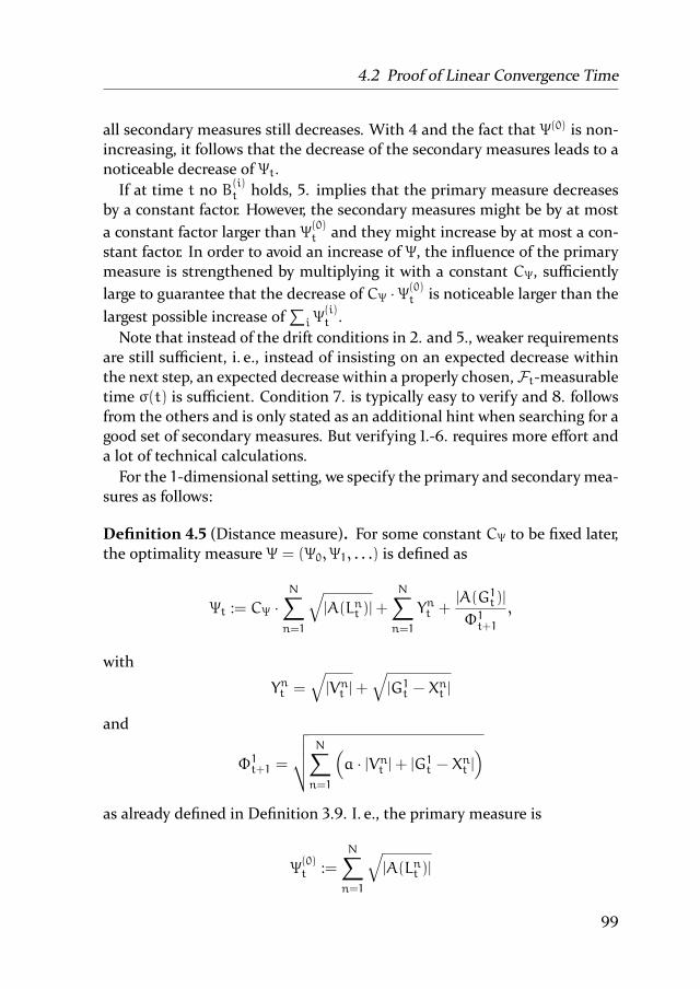
4.2 Proof of Linear Convergence Time
all secondary measures still decreases. With 4 and the fact that Ψ(0)is non-
increasing, it follows that the decrease of the secondary measures leads to a
noticeable decrease of Ψt.
If at time t no B(i)t holds, 5. implies that the primary measure decreases
by a constant factor. However, the secondary measures might be by at most
a constant factor larger than Ψ(0)t and they might increase by at most a con-
stant factor. In order to avoid an increase of Ψ, the influence of the primary
measure is strengthened by multiplying it with a constant CΨ, sufficiently
large to guarantee that the decrease of CΨ ·Ψ(0)t is noticeable larger than the
largest possible increase of
∑i Ψ
(i)t .
Note that instead of the drift conditions in 2. and 5., weaker requirements
are still sufficient, i. e., instead of insisting on an expected decrease within
the next step, an expected decrease within a properly chosen,Ft-measurable
time σ(t) is sufficient. Condition 7. is typically easy to verify and 8. follows
from the others and is only stated as an additional hint when searching for a
good set of secondary measures. But verifying 1.-6. requires more effort and
a lot of technical calculations.
For the 1-dimensional setting, we specify the primary and secondarymea-
sures as follows:
Definition 4.5 (Distance measure). For some constant CΨ to be fixed later,
the optimality measure Ψ = (Ψ0, Ψ1, . . .) is defined as
Ψt := CΨ ·N∑n=1
√|A(Lnt )|+
N∑n=1
Ynt +|A(G1t)|
Φ1t+1,
with
Ynt =√|Vnt |+
√|G1t − X
nt |
and
Φ1t+1 =
√√√√ N∑n=1
(a · |Vnt |+ |G1t − X
nt |)
as already defined in Definition 3.9. I. e., the primary measure is
Ψ(0)t :=
N∑n=1
√|A(Lnt )|
99
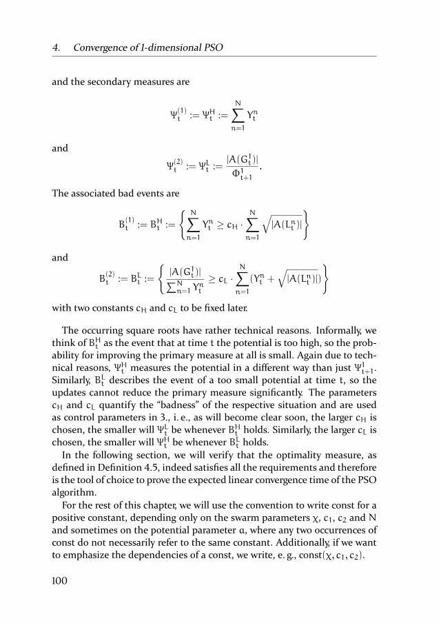
4. Convergence of 1-dimensional PSO
and the secondary measures are
Ψ(1)t := ΨHt :=
N∑n=1
Ynt
and
Ψ(2)t := ΨLt :=
|A(G1t)|
Φ1t+1.
The associated bad events are
B(1)t := BHt :=
N∑n=1
Ynt ≥ cH ·N∑n=1
√|A(Lnt )|
and
B(2)t := BLt :=
|A(G1t)|∑Nn=1 Y
nt
≥ cL ·N∑n=1
(Ynt +√|A(Lnt )|)
with two constants cH and cL to be fixed later.
The occurring square roots have rather technical reasons. Informally, we
think of BHt as the event that at time t the potential is too high, so the prob-
ability for improving the primary measure at all is small. Again due to tech-
nical reasons, ΨHt measures the potential in a different way than just Ψ1t+1.
Similarly, BLt describes the event of a too small potential at time t, so the
updates cannot reduce the primary measure significantly. The parameters
cH and cL quantify the “badness” of the respective situation and are used
as control parameters in 3., i. e., as will become clear soon, the larger cH is
chosen, the smaller will ΨLt be whenever BHt holds. Similarly, the larger cL is
chosen, the smaller will ΨHt be whenever BLt holds.
In the following section, we will verify that the optimality measure, as
defined in Definition 4.5, indeed satisfies all the requirements and therefore
is the tool of choice to prove the expected linear convergence time of the PSO
algorithm.
For the rest of this chapter, we will use the convention to write const for a
positive constant, depending only on the swarm parameters χ, c1, c2 and N
and sometimes on the potential parameter a, where any two occurrences of
const do not necessarily refer to the same constant. Additionally, if we want
to emphasize the dependencies of a const, we write, e. g., const(χ, c1, c2).
100

4.2 Proof of Linear Convergence Time
4.2.2 Lower Bounds for the Decrease of the Distance Measure
We need to examine the three measures ΨHt , ΨLt and Ψ
(0)t in order to verify
that they decrease sufficiently fast whenever the according event occurs and
that they never increase too fast. While the general bounds on the increase
of the according measures are in most cases intuitively clear, it is not obvi-
ous that, e. g., in case of a very high potential, ΨHt reduces sufficiently fast.
Therefore, before we present the formal proofs, we perform experiments to
illustrate that the stated measures are indeed a good choice and yield the
desired behavior.
High Potential
The first case is that the swarm potential is too large, i. e., much larger than
the areas that yield an improvement for either the global or the local attrac-
tor. In Section 3.5.2, a convergence analysis was presented, showing that un-
der the assumption of constant and identical attractors, the potential of the
swarm converges with linear convergence speed towards 0. To verify that this
result is stable, i. e., that the potential still decreases sufficiently fast if the
attractors are not constant but can move only inside an area which is small
compared to the swarm potential, we perform an experiment to see how the
swarm behaves when its attractors are very close to the optimum while the
potential is comparatively high.
In order to study the behavior of a swarm with a too high potential, we
choose two objective functions, namely SPHERE, defined as
SPHERE(x) = x2,
and SPHERE+([LW11]), defined as
SPHERE+(x) =
SPHERE(x), if x ≥ 0,∞, otherwise.
The functions can be seen in Figure 4.8a and Figure 4.8b.
In case of SPHERE,A(z) is for every z ∈ R a symmetric interval around the
optimum 0, while for the function SPHERE+, the optimum is at the upper
bound of the interval A(z) for every z ∈ R, z ≥ 0.
101

4. Convergence of 1-dimensional PSO
-10 -8 -6 -4 -2 0 2 4 6 8 100
10
20
30
40
50
60
70
80
90
100
(a) 1-dimensional function SPHERE.
-10 -8 -6 -4 -2 0 2 4 6 8 100
10
20
30
40
50
60
70
80
90
100
(b) 1-dimensional function SPHERE+.
Figure 4.8: The symmetric function SPHERE and the asymmetric function
SPHERE+.
Experiment 4.2. For each of the two objective functions, we use the swarm
sizes N = 2 and N = 10. We initialize the velocities uniformly at random
over [−100, 100] and choose the particles’ starting positions from the interval
[−10−100, 10−100] in case of SPHERE and [0, 10−100] in case of SPHERE+. I. e.,
the distance to the optimum is smaller than 10−100, while the velocities are
of order 100 and therefore the potential is comparatively high. Figure 4.9
shows the obtained values for ΨHt . We can see that indeed the potential of
the swarm increases with a speed neither depending much on the objective
function nor on the number of particles. Since the updates of attractors are
the only way the swarm reacts on the objective function, and since in the
configuration with a too high potential attractor updates happen too seldom
to have high influence on the swarm’s movement, the behavior is the same
for both (and any other) objective functions.
Regarding the influence of the swarm size, the swarm with only two par-
ticles apparently decreases its potential slightly faster than the swarm with
10 particles. The reason for this is that the measure ΨHt sums up all the po-
tentials of the single particles and is therefore only a constant factor smaller
than the maximum potential over all particles. Since the particles move (al-
most) independently of each other, ΨHt behaves similar to the maximum of
N independent random variables and therefore increases withN even if the
distribution of the particles’ potentials itself remains unchanged.
Indeed, the analysis from Section 3.5.2 can be extended to cover the case
where the attractors are not constant but can move not further than a dis-
tance that is small in comparison to the current potential. We formally prove
102

4.2 Proof of Linear Convergence Time
0 200 400 600 800 1000 1200 1400 1600 1800 200010-40
10-35
10-30
10-25
10-20
10-15
10-10
10-5
100
105
(a) Particles processing SPHERE after be-
ing initialized with a too high poten-
tial.
0 200 400 600 800 1000 1200 1400 1600 1800 200010-40
10-35
10-30
10-25
10-20
10-15
10-10
10-5
100
105
(b) Particles processing SPHERE+
after
being initialized with a too high po-
tential.
Figure 4.9: Particle swarm suffering from too high potential while process-
ing 10-dimensional objective functions SPHERE and SPHERE+
with N = 2 or N = 10 particles, initialized with 1 or D/2 di-
mensions with too high potential.
the observation from Experiment 4.2 in the following lemma, which verifies
1.-4. for BHt .
Lemma 4.2. There are constants t ′H ∈ N, c ′H > 0, CH > 0, δH ∈ (0, 1) andconstH, depending only on c1, c2, χ andN, such that for every t0 ∈ N, every
tH ≥ t0 + t ′H and every cH > c′H, we have
E
[N∑n=1
YntH
∣∣ Ft0]≤ CH ·
(N∑n=1
Ynt0 +
N∑n=1
√|A(Lnt0)|
), (4.2)
E
[N∑n=1
YntH
∣∣ Ft0 , BHt0]≤ (1− δH) ·
N∑n=1
Ynt0 , (4.3)
BHt0 implies |A(G1t0+1)|/Φ1t0+1≤ constH · Ψt0/cH, (4.4)
BHt0 implies
N∑n=1
Ynt0 ≥ Ψt0/(1+
CΨ + constH
cH
). (4.5)
Proof. To shorten notation, we write Et0 [ ] is E[ ∣∣ Ft0 ], analogous Vart0 [ ]
and Covt0 [ ]. In order to use the results from Section 3.5.2, we first concen-
103

4. Convergence of 1-dimensional PSO
trate only on a single particle n and express Et0 [YntH] in terms of expectation
and variance without absolute value inside:
Et0
[√|VntH |+
√|G1tH − XntH |
]≤
√Et0 [|V
ntH|] +
√Et0 [|G
1tH
− XntH |]
≤√|Et0 [V
ntH]|+
√Vart0 [V
ntH] (4.6)
+
√|Et0 [G
1tH+1
− XntH ]|+√
Vart0 [G1tH
− XntH ],
where for the first inequality we applied Jensen’s inequality and the second
inequality follows from
E[|Z|] ≤ E[|Z− E[Z]|+ |E[Z]|]
≤√
E[(Z− |E[Z]|)2] + |E[Z]| =√
Var[Z] + |E[Z]|,
which follows from the triangle inequality and the generalizedmean inequal-
ity.
It remains to bound the expectation and the variance of the velocity and
the distance to the global attractor. The same task was done by Jiang et al. in
[JLY07a] under the assumption of constant local and global attractors. In this
situation here, the attractors are not constant but their movement is limited:
The local attractor of particle n can not leave A(Lnt ) and the global attractor
is as least as good as any local, so it will also stay inside every A(Lnt ). With
this observation, we can modify the analysis from Section 3.5.2 as follows.
From the movement equations, we obtain for every t ∈ N.(Xnt+1Xnt
)=
(1+ χ− c1+c2
2 −χ1 0
)︸ ︷︷ ︸
=:A
·(XntXnt−1
)+
(c1 · rnt · Lnt + c2 · snt ·Gnt
0
)
By iterating, we get
(XntHXntH−1
)= AtH−t0 ·
(Xnt0Xnt0−1
)+
tH−t0−1∑t=0
Ai ·(c1 ·rnt0+t ·L
nt0+t
+ c2 ·snt0+t ·Gnt0+t
0
)
104

4.2 Proof of Linear Convergence Time
and therefore∥∥∥∥( Et0 [XntH]
Et0 [XntH−1
]
)∥∥∥∥1
=
∥∥∥∥∥AtH−t0 ·(Xnt0Xnt0−1
)+1
2·th−t0−1∑t=0
At ·(Et0 [c1 · Lnt0+t + c2 ·G
nt0+t
]
0
)∥∥∥∥∥1
≤ ‖Q‖1 · |λmax|th−t0 · ‖Q−1‖1
∥∥∥∥( XntXnt0−1
)∥∥∥∥1
+1
2· ‖Q‖1 ·
1
1− |λmax|· ‖Q−1‖1 · (c1 + c2) · |A(Lnt0)|,
whereQ is an invertible matrix such that A = Q ·D ·Q−1for some diagonal
matrixD and λmax is an eigenvalue ofAwith largest absolute value. Note that
the parameter guidelines for χ, c1 and c2 suggested in [JLY07a] guarantee
|λmax| < 1. Since Xnt−1 = X
nt − V
nt , we have
|Et0 [XntH]|+ |Et0 [V
ntH]|
≤ 2 · (|Et0 [XntH]|+ |Et0 [X
ntH
− VntH ]|)
≤ 1
2· c(χ, c1, c2) · (|λmax|
tH−t0 · (|Xnt0 |+ |Xnt0 − Vnt0|) + |A(Lnt0)|)
≤ c(χ, c1, c2) · (|λmax|tH−t0 · (|Xnt0 |+ |Vnt0 |) + |A(Lnt0)|) (4.7)
with a constant c(χ, c1, c2), depending only on χ, c1 and c2.
Analogous calculations show that also for the variance√Vart0 [X
ntH] +√
Vart0 [VntH]
≤ c ′(χ, c1, c2) · (|λ ′max|tH−t0 · (|Xnt0 |+ |Vnt0 |) + |A(Lnt0)|)
(4.8)
holds for some λ ′max
with |λ ′max
| < 1 and some constant c ′(χ, c1, c2). This
will turn out to yield a sufficient bound for the first square root in Equation
(4.6).
Now, we are going to bound the expected difference between the position
and the global attractor at time tH:
|Et0 [G1tH
− XntH ]| ≤ |A(Lnt0)|+ |Et0 [XntH]|
≤ |A(Lnt0)|+ c(χ, c1, c2) · (|λmax|tH−t0 · (|Xnt0 |+ |Vnt0 |) + |A(Lnt0)|)
≤ c ′′(χ, c1, c2) · (|λmax|tH−t0 · (|Xnt0 |+ |Vnt0 |) + |A(Lnt0)|) (4.9)
105
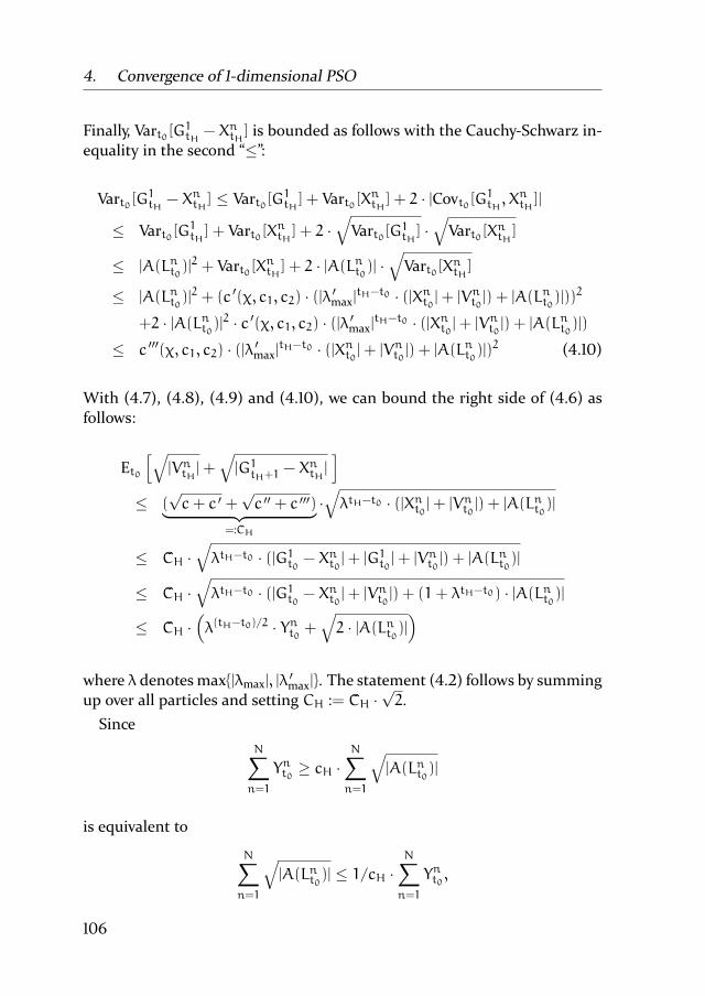
4. Convergence of 1-dimensional PSO
Finally, Vart0 [G1tH
− XntH ] is bounded as follows with the Cauchy-Schwarz in-
equality in the second “≤”:
Vart0 [G1tH
− XntH ] ≤ Vart0 [G1tH] + Vart0 [X
ntH] + 2 · |Covt0 [G
1tH, XntH ]|
≤ Vart0 [G1tH] + Vart0 [X
ntH] + 2 ·
√Vart0 [G
1tH] ·√
Vart0 [XntH]
≤ |A(Lnt0)|2 + Vart0 [X
ntH] + 2 · |A(Lnt0)| ·
√Vart0 [X
ntH]
≤ |A(Lnt0)|2 + (c ′(χ, c1, c2) · (|λ ′max
|tH−t0 · (|Xnt0 |+ |Vnt0 |) + |A(Lnt0)|))2
+2 · |A(Lnt0)|2 · c ′(χ, c1, c2) · (|λ ′max
|tH−t0 · (|Xnt0 |+ |Vnt0 |) + |A(Lnt0)|)
≤ c ′′′(χ, c1, c2) · (|λ ′max|tH−t0 · (|Xnt0 |+ |Vnt0 |) + |A(Lnt0)|)
2(4.10)
With (4.7), (4.8), (4.9) and (4.10), we can bound the right side of (4.6) as
follows:
Et0
[√|VntH |+
√|G1tH+1 − X
ntH|]
≤ (√c+ c ′ +
√c ′′ + c ′′′)︸ ︷︷ ︸
=:CH
·√λtH−t0 · (|Xnt0 |+ |Vnt0 |) + |A(Lnt0)|
≤ CH ·√λtH−t0 · (|G1t0 − X
nt0|+ |G1t0 |+ |Vnt0 |) + |A(Lnt0)|
≤ CH ·√λtH−t0 · (|G1t0 − X
nt0|+ |Vnt0 |) + (1+ λtH−t0) · |A(Lnt0)|
≤ CH ·(λ(tH−t0)/2 · Ynt0 +
√2 · |A(Lnt0)|
)where λ denotes max|λmax|, |λ
′max
|. The statement (4.2) follows by summing
up over all particles and setting CH := CH ·√2.
Since
N∑n=1
Ynt0 ≥ cH ·N∑n=1
√|A(Lnt0)|
is equivalent to
N∑n=1
√|A(Lnt0)| ≤ 1/cH ·
N∑n=1
Ynt0 ,
106

4.2 Proof of Linear Convergence Time
we have
Et0
[N∑n=1
√|VntH |+
√|G1tH − XntH |
∣∣ N∑n=1
Ynt0 ≥ cH ·N∑n=1
√|A(Lnt0)|
]
≤ CH ·(λ(tH−t0)/2 +
1
cH
)·N∑n=1
Ynt0 ≤ (1− δH) ·N∑n=1
Ynt0
with δH := 1 − CH ·(λ(tH−t0)/2 + 1
cH
). If cH ≥ 4 · CH =: c ′H and tH − t0 ≥
d2 · log(4 ·CH)/ log(1/λ)e =: t ′H, then δH ≥ 1/2. That proves statement (4.3).
Additionally, from
∑Nn=1 Y
nt0≥ cH ·
∑Nn=1
√|A(Lnt0)|, it follows that
|A(G1t0)|/Φ1t0+1
= |A(G1t0+1)|/
√√√√ N∑n=1
(a · |Vnt0 |+ |G1t0 − Xnt0|)
≤√2 ·N ·maxa, 1 · |A(G1t0)|/
N∑n=1
(√|Vnt0 |+
√|G1t0 − X
nt0|
)
≤√2 ·N ·maxa, 1 · |A(G1t0)|/
(cH ·
N∑n=1
√|A(Lnt0)|
)
≤√2 ·maxa, 1
cH·N∑n=1
√|A(Lnt )| ≤ constH · Ψt/cH,
where constH :=√2 ·maxa, 1. That finishes the proof of statement (4.4).
Finally, we have that
Ψt0 = CΨ ·N∑n=1
√|A(Lnt0)|+
N∑n=1
Ynt0 +|A(G1t0)|
Φ1t0+1
≤ CΨcH·N∑n=1
Ynt0 +
N∑n=1
Ynt0 +const
cH·N∑n=1
Ynt0 ,
i. e.,
∑Nn=1 Y
nt0≥ Ψt0/(1 +
CΨ+constHcH
). That finishes the proof of statement
(4.5).
107
4. Convergence of 1-dimensional PSO
Low Potential
Our next goal is to examine the case when the potential is too small, such
that updates of the attractors happen frequently but themovement and there-
fore the decrease of |A(Gnt )| is insignificant. This happens if every particle
has velocity and distance to both attractors much smaller than the distance
to the optimum, i. e., the whole swarm is gathered close to a non-optimal
point. In Section 4.1.1, we have proved that this situation is not stable, i. e.,
the swarm enters a state in which every velocity points towards the optimum
and every particle updates its local attractor in every step. We called this state
running and we have shown that for an appropriate parameter choice, during
this state the potential increases exponentially.
For different parameter sets, we have provided experimental evidence in
Experiment 4.1 that even for a small number of particles, the swarm ac-
celerates. Here, we repeat a similar experiment. But instead of compar-
ing different parameter sets, we keep the standard parameters of this thesis
(χ = 0.72984, c1 = c2 = 1.496172) while the number of particles varies.
Experiment 4.3. We initialize the particles uniformly over [−100, 100] anduse the objective function f(x) = −x, which obviously has no local optimum
and is therefore useful for simulating the situation of a local optimumwhich
is far out of reach. Figure 4.10 shows the measured courses of the potentials
for swarm sizes from N = 2 to N = 10. We can see that the potentials
indeed increase exponentially. In contrast to the case of a high potential, the
number of particles indeed matters. Figure 4.10 clearly shows that with a
larger swarm size, the swarm charges potential faster and is therefore able to
heal itself faster from encountering the bad event BLt .
By reusing the result of Section 4.1.1, we can formally show that in presence
of a too small potential, the term ΨLt satisfies the desired condition, i. e., it
decreases sufficiently fast. The following lemma verifies 1.-4. for BLt .
Lemma 4.3. There are constants t ′L ∈ N, c ′L > 0, CL > 0, δL ∈ (0, 1) andconstL, depending only on c1, c2, χ andN, such that there is for every t0 ∈ N
108

4.2 Proof of Linear Convergence Time
0 200 400 600 800 1000 1200 1400 1600 1800 2000100
1050
10100
10150
10200
10250
10300
10350
10400
10450
10500
N=2
N=3
N=4
N=5
N=6
N=7
N=8
N=9
N=10
Figure 4.10: Particle swarm suffering from too low potentials while process-
ing the 1-dimensional objective function f(x) = −xwith swarm
sizes between N = 2 and N = 10 particles.
a Ft0-measurable time σL with t0 ≤ σL ≤ t0+ t ′L almost surely, such that for
every cL > c′L and every tL ≥ t0, the following statements are fulfilled.
E
[|A(G1tL)|
Φ1tL+1
∣∣ Ft0]≤ CtL−t0L ·
|A(G1t0+1)|
Φ1t0, (4.11)
E
[|A(G1σL)|
Φ1σL+1
∣∣ Ft0 , BLt]≤ (1− δL) ·
|A(G1t0)|
Φ1t0+1, (4.12)
BLt implies
N∑n=1
Ynt0 ≤ constL · Ψt0/cL, (4.13)
BLt implies
|A(G1t0+1)|
Φ1t0+1≥ Ψt01+ constL · CΨ/cL
. (4.14)
Proof. First, we establish the bound of the expected increase of |A(Gnt )|/Φ1t
without any further knowledge in order to prove statement (4.11). Since
|A(Gnt )| is non-increasing over time, we only need to bound Et0 [1/ΦntH+1
].First, the focus lies only on a single step of just one particle of the swarm.
109

4. Convergence of 1-dimensional PSO
In order to simplify notation, we consider without loss of generality parti-
cle 1 as the one particle that is moved. The step of particle 1 can effect the
contributions of the other particles, if it updates the global attractor and
brings it closer to their positions. Therefore, a distinction between two cases
is made: The first case is that the contribution of particle 1 to the potential
is insignificant, so its step can only change the global attractor a little. In the
second case, particle 1 has a high contribution to the swarm potential. In
that case, its step might decrease the contributions of the other particles by
an arbitrary amount, but its own contribution decreases only within certain
bounds, therefore the whole swarm has a constant fraction of its potential
left. Let t ∈ N be an arbitrary point in time.
Case 1: The swarm potential is much larger than the potential of particle
1. More precisely:
N∑n=1
|G1t−1−Xnt−1| ≥ 2 ·N ·(χ · |V1t−1|+c1 · |L1t−1−X1t−1|+(c2+1) · |G1t−1−X1t−1|).
Since
|G1t−1 − Xnt−1| ≥ |G1t−1 − X
nt−1|− |G1t−1 − G
1t−1|
≥ |G1t−1 − Xnt−1|− |G1t−1 − X
1t |
≥ |G1t−1 − Xnt−1|− |G1t−1 − X
1t−1|− |X1t − X
1t−1|
= |G1t−1 − Xnt−1|− |G1t−1 − X
1t−1|− |V1t |
≥ |G1t−1 − Xnt−1|− χ · |V1t−1|− c1 · |L1t−1 − X1t−1|
−(c2 + 1) · |G1t−1 − X1t−1|,
we have
N∑n=1
|G1t−1 − Xnt−1|
≥N∑n=1
(|G1t−1 − X
nt−1|− χ · |V1t−1|− c1 · |L1t−1 − X1t−1|
− (c2 + 1) · |G1t−1 − X1t−1|)
110

4.2 Proof of Linear Convergence Time
=1
2·N∑n=1
|G1t−1 − Xnt−1|+
1
2·N∑n=1
|G1t−1 − Xnt−1|−N · χ · |V1t−1|
−N · c1 · |L1t−1 − X1t−1|−N · (c2 + 1) · |G1t−1 − X1t−1|
≥ 12·N∑n=1
|G1t−1 − Xnt−1|
This observation leads to
Φ1t =
√√√√a|V1t |+ |G1t−1 − X1t |+
N∑n=2
(a|Vnt−1|+ |G1t−1 − X
nt−1|)
≥
√√√√1
2|G1t−1 − X
1t |+
N∑n=2
(a|Vnt−1|+
1
2|G1t−1 − X
nt−1|
)
≥√1
2·
√√√√|G1t−1 − X1t |+
N∑n=2
(a|Vnt−1|+ |G1t−1 − X
nt−1|).
On the other hand, we have
Φ1t =
√√√√ N∑n=1
a|Vnt−1|+ |G1t−1 − Xnt−1|
≤
√√√√a|V1t−1|+ |G1t−1 − X1t−1|+
N∑n=2
(a|Vnt−1|+ |G1t−1 − X
nt−1|)
≤
√√√√(1+ a
2Nχ
)|G1t−1 − X
1t−1|+
N∑n=2
(a|Vnt−1|+
a
2Nχ|G1t−1 − X
nt−1|
)
≤
√(1+
a
2Nχ
)·
√√√√|G1t−1 − X1t−1|+
N∑n=2
(a|Vnt−1|+ |G1t−1 − X
nt−1|).
It follows that
Φ1t ≥ Φ1t/√2 · (1+ a/(2 ·N · χ))
and therefore
Et−1[1/Φ1t ] ≤
√2 · (1+ a/(2 ·N · χ))/Φ1t .
111

4. Convergence of 1-dimensional PSO
Case 2: Particle 1 contributes significantly to the swarm potential. More
precisely:
N∑n=1
|G1t−1−Xnt−1| < 2 ·N ·(χ · |V1t−1|+c1 · |L1t−1−X1t−1|+(c2+1) · |G1t−1−X1t−1|).
Since particle 1 might be able to bring the global attractor closer to the
other particles, we cannot rely on their old distances to the global attractor
as a lower bound for the swarm potential after the step of particle 1. However,
the velocities of the remaining swarm members will stay the same. For the
potential after the step of particle 1, that means
Φ1t = a|V1t |+ |G1t−1 − X1t |+
N∑n=2
(a|Vnt−1|+ |G1t−1 − X
nt−1|)
≥ a|V1t |+ |G1t−1 − X1t |+
N∑n=2
a|Vnt−1|.
On the other hand, the portion of the potential that comes from the dis-
tances of the particles 2, . . . ,N to the global attractor, i. e., the part that can
actually vanish is exactly the part that is bounded in terms of the contribu-
tion of particle 1 to the potential:
Φ1t =
N∑n=1
a|Vnt−1|+ |G1t−1 − Xnt−1|
≤ 2 ·N ·(χ · |V1t−1|+ c1 · |L1t−1 − X1t−1|+ (c2 + 1) · |G1t−1 − X1t−1|
)+a|V1t−1|+
N∑n=2
a|Vnt−1|.
By setting
b1 := 2 ·N · (χ · |V1t−1|+ c1 · |L1t−1 − X1t−1|+ (c2 + 1) · |G1t−1 − X1t−1|)
+ a · |V1t−1|+N∑n=2
a · |Vnt−1|,
b2 := a|V1t |+ |G1t−1 − X
1t |,
c :=
N∑n=2
a|Vnt−1|,
112

4.2 Proof of Linear Convergence Time
and with the generalized weighted mean inequality, we obtain
Et−1[Φ1t/Φ
1t ]
≤ Et−1
√√√√2N(χ|V1t−1|+ c1|L1t−1 − X
1t−1|+ (c2 + 1)|G
1t−1 − X
1t−1|)
a|V1t |+ |G1t−1 − X1t |+∑Nn=2 a|V
nt−1|
+a|V1t−1|+
∑Nn=2 a|V
nt−1|
a|V1t |+ |G1t−1 − X1t |+∑Nn=2 a|V
nt−1|
= Et−1
[√b1 + a
b2 + a
]
≤ Et−1
[w ·
√b1b2
+ (1−w) ·√a
a
]= w · Et−1
[√b1b2
]+ (1−w)
for w = b1/(b1 + a) ≤ 1. Note that w is Ft−1-measurable. The term
Et−1[√b1/b2] is bounded in the following way:
Et−1
[√b1b2
]
= Et−1
[√2 ·N · (χ · |V1t−1|+ c1 · |L1t−1 − X1t−1|+ (c2 + 1) · |G1t−1 − X1t−1|)
a · |V1t |+ |G1t−1 − X1t |
+a|V1t−1|
a · |V1t |+ |G1t−1 − X1t |
]
≤ Et−1
√2 ·N · (χ · |V1t−1|+ c1 · |L1t−1 − X1t−1|+ (c2 + 1) · |G1t−1 − X1t−1|)a · |V1t |
+a · |V1t−1|a · |V1t |
]
= Et−1
[√2 ·N · (χ · |V1t−1|+ c1 · |L1t−1 − X1t−1|+ (c2 + 1) · |G1t−1 − X1t−1|)a · |χ · |V1t−1|+ c1 · r1t · (L1t−1 − X1t−1) + c2 · s1t · (G1t−1 − X1t−1)|
+a · |V1t−1|
a · |χ · |V1t−1|+ c1 · r1t · (L1t−1 − X1t−1) + c2 · s1t · (G1t−1 − X1t−1)|
]
113
4. Convergence of 1-dimensional PSO
≤√4 ·N/a+ 1/χ·
· Et−1
[√χ · |V1t−1|+ c1 · |L1t−1 − X1t−1|+ c2 · |G1t−1 − X1t−1|
|χ · |V1t−1|+ c1 · r1t · (L1t−1 − X1t−1) + c2 · s1t · (G1t−1 − X1t−1)|
].
The remaining expectation leads to an expression of the form∫ 10
∫ 10
√1
|x+ r · y+ s · z|drds
with |x|+|y|+|z| = 1, which is, as straight-forward calculations show, bounded
by some constant.
Both cases together show that on expectation the reciprocal of the swarm
potential increases by at most a constant factor during a single step. There-
fore, it also increases on expectation by at most a constant factor during a
complete iteration. That finishes the proof of statement (4.11).
The next goal is to verify the improved bound for the case of a very small
swarm potential. For simplicity, we use the notation
EL[ ] := Et0
[∣∣ |A(G1t0)|/ N∑
n=1
Ynt0 ≥ cL ·N∑n=1
(Ynt0 +
√|A(Lnt0)|
)],
PL( ) is used analogously. Note that
|A(G1t0)|/
N∑n=1
Ynt0 ≥ cL ·N∑n=1
(Ynt0 +
√|A(Lnt0)|
)implies
|A(G1t0)|/
N∑n=1
Ynt0 ≥ cL ·N∑n=1
Ynt0
and therefore
|A(G1t0)| ≥ cL ·( N∑n=1
Ynt0
)2≥ cL ·
N∑n=1
(|Vnt0 |+ |G1t0 − Xnt0|).
In particular, for cL > 1, the condition implies that sign(G1t0) = sign(Xnt ) forevery particle n. Without loss of generality, we can assume that for every n
114

4.2 Proof of Linear Convergence Time
Xnt0 < G1t0< 0. First, we check that a large distance between a particle and
its local attractor increases the particles Y-value on expectation even within
a single step. Consider the case of |Ln0t0 − Xn0t0 | > 9 · N/c1 · |A(G1t0)|/cL for
some particle n0. Then, we have
EL
[Φ1t0+1
Φ1t0+2
∣∣ |Lnt0 − Xnt0 | ≥ 9 ·N/c1 · |A(G1t0)|/cL]
≤ EL
[√2 ·N ·
∑Nn=1 Y
nt0
|Vn0t+1|
∣∣ |Lnt0 − Xnt0 | ≥ 9 ·N/c1 · |A(G1t0)|/cL]
≤ sup
sn0t0∈[0,1]
∫ 10
√2 ·N ·
∑Nn=1 Y
nt0
|χ·Vn0t0 + c1 ·rn0t0 ·(Ln0t0
− Xn0t0 ) + c2 ·sn0t0·(Gn0t0 − Xn0t0 )|
drn0t0+1
≤ sup
sn0t0∈[0,1]
(√2 ·N ·
N∑n=1
Ynt0
)· 2/(c1 · (Ln0t0 − Xn0t0 ))·
·(√
|c1 · (Ln0t0 − Xn0t0 ) − χ · Vn0t0
− c2 · sn0t0 · (Gn0t0
− Xn0t0 )|
−√|χ · Vn0t0 + c2 · sn0t0 · (G
n0t0
− Xn0t0 )|)
≤
(√8 ·N ·
N∑n=1
Ynt0
)·
√c1 · (Ln0t0 − Xn0t0 ) + χ · |V
n0t0
|
c1 · (Ln0t0 − Xn0t0 )
≤
√8 ·N ·√
|A(G1t0)|
cL
·√c1 · (Ln0t0 − Xn0t0 ) + χ ·
(∑Nn=1 Y
nt0
)2c1 · (Ln0t0 − Xn0t0 )
≤
√8 ·N ·√c1 · (Ln0t0 − Xn0t0 )
9 ·N
·√c1 · (Ln0t0 − Xn0t0 ) + χ · |A(G
1t0)|/cL
c1 · (Ln0t0 − Xn0t0 )
≤(√
8/9 ·√c1 · (Ln0t0 − Xn0t0 )
)·
√c1 · (Ln0t0 − Xn0t0 ) · (1+ 1/(9 ·N))
c1 · (Ln0t0 − Xn0t0 )
=√8/9 · 1+ 1/(9 ·N) < 1,
i. e., in this situation we can set σL := 1. For the rest of the proof, we assume
that |Ln0t0 −Xn0t0| ≤ 9·N/c1 ·|A(G1t0)|/cL. In particular, for a sufficiently large cL
this guarantees that the local attractors also have the same sign as the global
115
4. Convergence of 1-dimensional PSO
attractor, i. e., without loss of generality, we can assume that Xnt0 < Lnt0 <
G1t0 < 0 for every n.
There are two essentially different cases, depending on the shape of the
objective function f: Either, A(G1t0) has size about 2 · |G1t0 |, as it is the case
when processing, e. g., objective function SPHERE. Or |A(G1t0)| |G1t0 |. In
the first case, the particles have a large area on which the function is mono-
tone to accelerate. In the second case, the monotone area might be too small
for a decent acceleration of the particles, but after overcoming the optimum
at 0, the particles improve the global attractor significantly.
In the proof of Lemma 4.1 in Section 4.1.1, we have shown that on a mono-
tone area the particles do actually accelerate, as soon as they have entered a
certain constellation. More precise, we have shown that for proper choices
of the swarm parameters χ, c1, c2,N and of the parameter a of the potential
and every t ∈ N,
Et[Φnt /Φ
nt+1
∣∣ Ft, ∃ε ∈ −1, 1, ∀n : sign(Vnt ) = sign(G1t − Xnt ) = ε] ≤ q < 1
holds, where q depends only on χ, c1, c2, N and a.
The state “running” describes the situation when on a monotone area the
velocities all point towards the direction inwhich the function is falling. Note
that under such circumstances, themonotonicity of f implies that sign(Vnt ) =sign(G1t − X
nt ) = sign(Lnt − X
nt ) for every particle n.
Since the improvements of |A(G)|/Φ start as soon as either the swarm
gets running or it surpasses 0, the strategy for the proof of statement (4.12)
is to separate the expectation into two conditioned expectations, one that
assumes that the swarm either started running or reached a positive position
not later than at a certain iteration t0 + t′0 and one that assumes that the
swarm did neither of both until time t0 + t′0. Let the stopping time τ be the
first time ≥ t when at least one of the two events happens, namely when
either the swarm is running or it reaches a position > 0. We have
EL[|A(G1σL)|/Φ1σL+1]
= PL(τ ≤ t0 + t ′0) · EL[|A(G1σL)|/Φ1σL+1
∣∣ τ ≤ t0 + t ′0]+ PL(τ > t0 + t
′0) · EL[|A(G1σL)|/Φ
1σL+1
∣∣ τ > t0 + t ′0]≤ EL[|A(G
1σL)|/Φ1σL+1
∣∣ τ ≤ t0 + t ′0]+ PL(τ > t0 + t
′0) · EL[|A(G1σL)|/Φ
1σL+1
∣∣ τ > t0 + t ′0] (4.15)
In the following, we will bound each of the three remaining expressions,
starting with EL[|A(G1σL)|/Φ1σL+1
∣∣ τ > t0 + t ′0].116
4.2 Proof of Linear Convergence Time
Since the expectation EL[|A(G1σL)|/Φ1σL+1
∣∣ τ > t0 + t ′0] is conditioned, wecannot apply (4.11) for an upper bound. Instead, we prove a uniform bound
on the future swarm potential. This is possible because in the current situ-
ation, no particle can bring the global attractor closer to a different particle,
so each one can only damage its own contribution to the potential. The fol-
lowing calculations show that every iteration preserves at least a constant
fraction of the swarm potential. The updated values of particle n are
Vnt0+1 = χ · Vnt0+ c1 · rnt0+1 · (L
nt0− Xnt0) + c2 · s
nt0+1· (Gnt0 − X
nt0),
Xnt0+1 = Xnt0+ χ · Vnt0 + c1 · r
nt0+1· (Lnt0 − Xt0t
n) + c2 · snt0+1 · (Gnt0− Xnt0).
If Vnt0 is positive, it follows that
a · |Vnt0+1|+ |G1t0+1 − Xnt0+1
| ≥ a · |Vnt0+1| ≥ a · χ · |Vnt0|
and additionally
a · |Vnt0+1|+ |G1t0+1 − Xnt0+1
| = a · Vnt0+1 +G1t0+1
− Xnt0+1
≥ mina, 1 · (Vnt0+1 +Gnt0− Xnt0+1)
= mina, 1 · |Gnt0 − Xnt0|.
Since both bounds hold, any weighted mean of them is also a valid bound.
It follows
a · |Vnt0+1|+ |G1t0+1 − Xnt0+1
| ≥ mina, 1 · χmina, 1+ χ
· (a · |Vnt0 |+ |Gnt0 − Xnt0|).
If on the other hand Vnt0 is negative, two subcases need to be considered. If
−χ · Vnt0 ≥ (c1 + c2) · (Gnt0 − Xnt0), we have
−Vnt0+1 ≥ −χ · Vnt0 − c1 · rnt0+1· (Lnt0 − X
nt0) − c2 · snt0+1 · (G
nt0− Xnt0)
≥ −χ · Vnt0 − (c1 + c2) · (Gnt0 − Xnt0) ≥ 0,
G1t0+1 − Xnt0+1≥ Gnt0 − X
nt0− Vnt0+1.
Consequently, for the contribution to the potential, we have
a · |Vnt0+1|+ |G1t0+1 − Xnt0+1
| = −a · Vnt0+1 +G1t0+1
− Xnt0+1
= −(a+ 1) · Vnt0+1 +Gnt0− Xnt0
≥ −(a+ 1) · Vnt0+1 + 1/2 · (Gnt0− Xnt0) + 1/2 · (V
nt0+1
− χ · Vnt0)/(c1 + c2)≥ 1/2 · (Gnt0 − X
nt0) − χ/2 · 1/(c1 + c2) · Vnt0
≥ χ/2 · 1/(c1 + c2) ·min1, 1/a · (Gnt0 − Xnt0− a · Vnt0)
= χ/2 · 1/(c1 + c2) ·min1, 1/a · (a · |Vnt0 |+ |G1t0 − Xnt0|).
117

4. Convergence of 1-dimensional PSO
If −χ · Vnt0 < (c1 + c2) · (Gnt0 − Xnt0), we obtain
a · |Vnt0+1|+ |G1t0+1 − Xnt0+1
|
≥ mina, 1 · (Vnt0+1 +Gnt0+1
− Xnt0+1)
= mina, 1 · (Gnt0+1 − Xnt0)
≥ mina, 1 · (Gnt0 − Xnt0)
≥ mina, 1 · χ
χ+ a · (c1 + c2)(Gnt0 − X
nt0− a · Vnt0)
= mina, 1 · χ
χ+ a · (c1 + c2)(a · |Vnt0 |+ |Gnt0 − X
nt0|).
Putting both cases together and building the minimum over all appearing
constants leads to
Φ1t0+1 ≥ const ·Φ1t0 ,
where const = const(χ, c1, c2, a). This implies
EL[1/Φ1σL+1
∣∣ τ > t0 + t ′0] ≤ constt ′0 · CσL−t0−t
′0
L · 1/Φ1t0+1.
Now, we are going to bound the next term of (4.15), namely
EL[|A(G1σL)|/Φ1σL+1
∣∣ τ ≤ t0 + t ′0].Since the condition√
|A(G1t0)| ≥ cL ·N∑n=1
(√|Vnt0 |+
√G1t0 − X
nt0
)does not imply any lower bound on the number of iterations the swarm can
keep running, we first restrict the considerations to the case when
|Vnt0 |+ |G1t0 − Xnt0|+ |Lnt0 − X
nt0| ≤ |G1t0 |/
√cL
for every n. Since
|Vnt0+1| ≤ χ · |Vnt0|+ c1 · |Lnt0 − Xt0 |+ c2 · |G
1t0− Xnt0 |,
|Lnt0+1 − Xnt0+1
| ≤ |Lnt0 − Xnt0|+ |Vnt0+1|,
|G1t0+1 − Xnt0+1
| ≤ |G1t0 − Xnt0|+
N∑n ′=1
|Vn′
t0+1|,
118

4.2 Proof of Linear Convergence Time
during one iteration
∑Nn=1 |V
nt0|+ |Lnt0−X
nt0|+ |G1t0−X
nt0| increases by at most
a factor const that depends only on c1, c2, χ and N. Therefore, we have for
every particle n:
|Xnt0+t ′0−G1t0 | ≤ |G1t0 − X
nt0|+
t ′0−1∑l=1
|Vnt0+l|
≤ |G1t0 | · (1/√cL +
t ′0−1∑i=1
consti/√cL) < |G1t0 |
for t ′0 ≤log cL
log const. This implies that the swarm will for t ′0 ≤
log cLlog const
reach no
positive position at time t0 + t′0 and therefore still be running.
In combination with the results from Lemma 4.1 of Section 4.1.1, this leads
to
EL[|A(G1σL)|/Φ1σL+1
∣∣ τ ≤ t0 + t ′0] ≤ constt ′0 · qσL−t0−t ′0 · |A(G1t0)|/Φ
1t0+1
for t ′0 ≤log cL
log const.
It remains the case when
|Vnt0 |+ |Gnt0 − Xnt0|+ |Lnt0 − X
nt0| ≥ |G1t0 |/
√cL
for somen. If that is the case, we cannot expect a large increase ofΦ. Instead,
we can expect a large decrease of |A(G)| since after the swarm stops running,
|A(G)| ≤ const · |G1t0 | will hold. Note that
|A(G1t0)|/cL ≥N∑
n ′=1
|Vn′
t0|+ |Gn
′t0
− Xn′
t0|+ |Ln
′t0
− Xn′
t0|
implies here
|A(G1t0)| ≥√cL · |G1t0 |.
For our calculations regarding the decrease of |A(G1t0)|, we introduce a se-
quence of random variables (A ′t)t≥t0 , which has the constant value |A(G1t0)|until the first particle surpasses the optimum at 0. From that point in time
on, during each step of a particle A ′t decreases by a factor of q/CL, i. e., A′t
pays for the possible decrease of Φ and additionally it decreases by a factor
of q. For the formal analysis, A ′t is defined in the following way:
A ′t0 := |A(G1t0)|
A ′t+1 :=
A ′t, if ∀s, t0 ≤ s ≤ t, ∀n : sign(Xns ) = sign(X1t0),
A ′t · (q/CL)N, otherwise.
119

4. Convergence of 1-dimensional PSO
Similar to the previous case, we have
EL[A′σL/Φ1σL+1
∣∣ τ ≤ t0 + t ′0] ≤ constt ′0 · qσL−t0−t ′0 · |A(G1t0)|/Φ
1t0+1
.
Now, we have to show that
|A(G1t0+t)| ≤ A′t0+t
for every t ≤ const(χ, c1, c2, N) · log cL. Let t0 + τ0 denote the first time
when some particle surpasses 0. For t < τ0, |A(G1t0+t
)| ≤ A ′t0+t follows
directly from the definition of A ′. For t ≥ τ0, let n0 be the first particle that
overcame the optimum at 0. We have
|A(G1t0+t+1)| ≤ |A(Gn0t0+τ0+1)| ≤ |Xn0t0+τ0 − Xn0t0+τ0−1
| = |Vn0t0+τ0 |. (4.16)
As a bound for the velocity when overcoming 0, we have
|Vn0t0+τ0 | ≤ χ · |Xn0t0+τ0−1
− Xn0t0+τ0−2|+ c1 · (Ln0t0+τ0−1
− Xt0+τ0−1)
+ c2 · (Gn0t0+τ0−1 − Xn0t0+τ0−1
).(4.17)
Before the time t0+ τ0, the largest possible distance between the position of
some particle n and 0 is bounded from above by
|Xnt0 |+
∞∑t=0
χt · |Vnt0 | ≤ |G1t0 |+ |Xnt0 −G1t0|+ 1/(1− χ) · |Vnt0 |
≤ |G1t0 |+ 1/(1− χ) · |A(G1t0)|/cL
≤ const · |A(G1t0)|/√cL
for cL > 1. Therefore, we have for every n ≤ N and every s ≤ τ0
|Xnt0+s| ≤ const · |A(G1t0)|/√cL.
Since the global and local attractors are also former positions of some parti-
cles, this, together with (4.16) and (4.17), implies
|A(G1t0+t)| ≤ const · |A(G1t0)|/√cL.
From the definition of A ′, it follows that
A ′t0+t ≥ |A(G1t0)| · (q/CL)N·t.
120
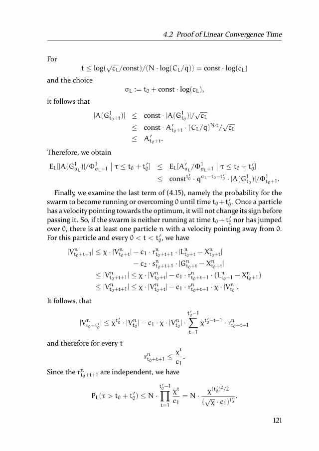
4.2 Proof of Linear Convergence Time
For
t ≤ log(√cL/const)/(N · log(CL/q)) = const · log(cL)
and the choice
σL := t0 + const · log(cL),it follows that
|A(G1t0+t)| ≤ const · |A(G1t0)|/√cL
≤ const ·A ′t0+t · (CL/q)N·t/√cL
≤ A ′t0+t.
Therefore, we obtain
EL[|A(G1σL)|/Φ1σL+1
∣∣ τ ≤ t0 + t ′0] ≤ EL[A′σL/Φ1σL+1
∣∣ τ ≤ t0 + t ′0]≤ const
t ′0 · qσL−t0−t ′0 · |A(G1t0)|/Φ1t0+1
.
Finally, we examine the last term of (4.15), namely the probability for the
swarm to become running or overcoming 0 until time t0+t′0. Once a particle
has a velocity pointing towards the optimum, it will not change its sign before
passing it. So, if the swarm is neither running at time t0+ t′0 nor has jumped
over 0, there is at least one particle n with a velocity pointing away from 0.
For this particle and every 0 < t < t ′0, we have
|Vnt0+t+1| ≤ χ · |Vnt0+t
|− c1 · rnt0+t+1 · |Lnt0+t
− Xnt0+t|
− c2 · snt0+t+1 · |Gnt0+t
− Xnt0+t|
≤ |Vnt0+t+1| ≤ χ · |Vnt0+t
|− c1 · rnt0+t+1 · (Lnt0+1
− Xnt0+1)
≤ |Vnt0+t+1| ≤ χ · |Vnt0+t
|− c1 · rnt0+t+1 · χ · |Vnt0|.
It follows, that
|Vnt0+t ′0| ≤ χt ′0 · |Vnt0 |− c1 · χ · |V
nt0| ·t ′0−1∑t=1
χt′0−t−1 · rnt0+t+1
and therefore for every t
rnt0+t+1 ≤χt
c1.
Since the rnt0+t+1 are independent, we have
PL(τ > t0 + t′0) ≤ N ·
t ′0−1∏t=1
χt
c1= N · χ(t
′0)2/2
(√χ · c1)t
′0
.
121

4. Convergence of 1-dimensional PSO
Putting things together, we obtain
EL[|A(G1σL)|/ΦnσL ] ≤ EL[|A(G
1σL)|/ΦnσL
∣∣ τ ≤ t0 + t ′0]+ PL(τ > t0 + t
′0) · EL[|A(G1σL)|/Φ
nσL
∣∣ τ > t0 + t ′0]≤ const
t ′0 · qσL−t0−t ′0 ·|A(G1t0)|
Φ1t0+1+
χ(t′0)2/2
(√χ · c1)t
′0
· constt ′0 ·|A(G1t0)|
Φ1t0+1
=
(const
t ′0 · qσL−t0−t ′0 + χ(t′0)2/2
(√χ · c1)t
′0
· constt ′0)·|A(G1t0)|
Φ1t0+1.
for every t ′0 ≤log cL
log const. To finish the proof of statement (4.12), we first choose
t ′0 sufficiently large, such that
χ(t′0)2/2
(√χ · c1)t
′0
· constt ′0 < 1/3.
Then, we choose σL sufficiently large to obtain constt ′0 ·qσL−t0−t ′0 < 1/3. The
value t ′ is set accordingly. Finally, we choose cL sufficiently large to guarantee
t ′0 ≤log cL
log const. Note that all the choices only depend on the fixed parameters
of the swarm, i. e., on χ, c1, c2, N, a and q which itself depends only on
the other swarm parameters. With the choice of δL := 1/3, the proof of
statement (4.12) is finished.
From
|A(G1t0)|∑N
n=1 Ynt0
≥ cL ·∑Nn=1(Y
nt0+√|A(Lnt0)|), it follows that
N∑n=1
Ynt0 ≤|A(G1t0)|
cL ·∑Nn=1 Y
nt0
=|A(G1t0)|
cL ·∑Nn=1(
√|Vnt |+
√|G1t − X
nt |)
≤|A(G1t0)|
cL ·√∑N
n=1(|Vnt |+ |G1t − X
nt |)
≤max
√a, 1 · |A(G1t0)|cL ·Φ1t+1
≤ max√a, 1 · Ψt0/cL.
That proves statement (4.13).
122

4.2 Proof of Linear Convergence Time
Finally,
|A(G1t0)|∑N
n=1 Ynt0
≥ cL ·∑Nn=1(Y
nt0+√|A(Lnt0)|) implies
Ψt0 = CΨ ·N∑n=1
√|A(Lnt0)|+
N∑n=1
Ynt0 +|A(G1t0)|
Φ1t0+1
≤ (CΨ + 1)/cL ·|A(G1t0)|∑Nn=1 Y
nt0
+|A(G1t0)|
Φ1t0+1
≤ max√a, 1 · (CΨ + 1)/cL ·
|A(G1t0)|
Φ1t0+1+
|A(G1t0)|
Φ1t0+1
= (max√a, 1 · (CΨ + 1)/cL + 1) ·
|A(G1t0)|
Φ1t0+1.
That finishes the proof of statement (4.14).
The Right Amount of Potential
The next step is to analyze the primary measure Ψ(0)t . The goal is to show
that when the potential is neither too high nor too low, the primary measure
indeed decreases on expectation by a factor of 1− δR. This is not surprisingand it can be clearly seen in experiments.
Experiment 4.4. We measure Ψ(0)t for N = 10 particles processing the ob-
jective functions SPHERE and SPHERE+after being initialized with positions
chosen randomly from [−100, 100] for SPHERE and from [0, 100] for SPHERE+
and with swarm sizes N = 2 and N = 10. The results can be seen in Figure
4.11. Indeed, the primary measure decreases exponentially over time. Sim-
ilar to the case of a too high potential, we can see that in case of the larger
swarm size Ψ(0)t decreases slightly slower.
While the claimed decrease of Ψ(0)t is intuitively clear since it only says
that the swarm indeed optimizes if it is not in a condition that prevents it
from optimizing, the formal proof turns out to yield some peculiarities and
a number of case distinctions is necessary.
Beforewe can verify 5. and 6., we state a rather technical lemma that shows
how a particle swarm with an appropriate potential level can hit its goal. Its
123

4. Convergence of 1-dimensional PSO
0 200 400 600 800 1000 1200 1400 1600 1800 200010-45
10-40
10-35
10-30
10-25
10-20
10-15
10-10
10-5
100
105
(a) Particles processing objective func-
tion SPHERE
0 200 400 600 800 1000 1200 1400 1600 1800 200010-45
10-40
10-35
10-30
10-25
10-20
10-15
10-10
10-5
100
105
(b) Particles processing objective func-
tion SPHERE+
Figure 4.11: Primary measure of a particle swarm processing the 1-
dimensional objective functions SPHERE and SPHERE+
with
swarm sizes N = 2 and N = 10.
proof consists of the explicit construction of sets of sequences of steps, that
have a sufficiently high probability and bring the particles into the area that
is substantially better than the current attractors.
Lemma 4.4. Let A = [a, b] be an interval containing 0, i. e., a ≤ 0 ≤ b.
Define
dL :=1
χ·max
2·(χ+1)χ·(c1−1) ,
4·χ+2·c2−2χ·(c2−1)
minχ, 1/3, (c2 − 1)/6
.
Assuming that
dL · sup
x∈A(Gnt )dist(x,A) ≤ |Vnt |+ |Gnt − X
nt |+ |Lnt − X
nt | ≤ dH · |A|
for some dH > 0, the probability for particle n to hit A within the next 3
steps is bounded from below by a constant const(dH, c1, c2, χ).
Proof. We divide the proof into three parts, depending on the number of
steps necessary to hit A. First, we cover configurations that allow the swarm
to hitAwithin a single step, even with some less restrictive bounds for |Vnt |+|Gnt − X
nt |+ |Lnt − X
nt |:
Claim 4.1. Given that
• |Vnt |+ |Gnt − Xnt |+ |Lnt − X
nt | ≤ 5
3 · ((3 ·maxc1, c2+ 1) · dH + 1) · |A|,
124

4.2 Proof of Linear Convergence Time
• |Vnt |+ |Gnt −Xnt |+ |Lnt −X
nt | ≥ max
2(χ+1)χ(c1−1)
, 4χ+2c2−2χ(c2−1)
· supx∈A(Gnt )
dist(x,A)
and
• Xnt ≤ 0 and−(Lnt −Xnt )−
c2−12 ·(G
nt −X
nt ) ≤ χ ·Vnt ≤ (a−Xnt )+ |A|/2 or
Xnt ≥ 0 and−(Lnt −Xnt )−
c2−12 · (G
nt −X
nt ) ≥ χ ·Vnt ≥ (b−Xnt )− |A|/2,
the probability for particle n hittingA within the next step is bounded from
below by a constant const(dH, c1, c2, χ).
Proof. Due to symmetry reasons, we can without loss of generality assume
that Xnt ≤ 0 and −(Lnt −Xnt ) −
c2−12 · (G
nt −X
nt ) ≤ χ ·Vnt ≤ (a−Xnt ) + |A|/2.
By straight-forward calculation, we can show that for any interval
I ⊂ [Xnt + χ · Vnt , Xnt + χ · Vnt + c1 · (Lnt − Xnt ) + c2 · (Gnt − Xnt )],
we have
Pt(Xnt+1 ∈ I) ≥
|I|2
2 · (c1 · (Lnt − Xnt ) + c2 · (Gnt − Xnt ))2. (4.18)
Therefore, all that remains to do is to find a sufficiently large I. Note that
due to to unimodality of the objective function, the position of a particle can
never be strictly between its local and the global attractor, i. e., for Xnt ≤ 0,the signs of Lnt −X
nt andGnt −X
nt are both non-negative. Therefore, the area
that can actually be reached by particle n within its next step is
R := [Xnt + χ · Vnt , Xnt + χ · Vnt + c1 · (Lnt − Xnt ) + c2 · (Gnt − Xnt )],
so we need to bound |R∩A|. First, we consider the case Vnt < 0. In that case,
the highest point reachable by particle n is the interval
Xnt + χ · Vnt + c1 · (Lnt − Xnt ) + c2 · (Gnt − Xnt )= Gnt + χ · Vnt + c1 · (Lnt − Xnt ) + (c2 − 1) · (Gnt − Xnt )≥ Gnt + χ · Vnt + c1 · (Lnt − Xnt ) + (c2 − 1) · (Gnt − Xnt )
−min
χ+ c1χ+ 1
,χ+ c2 − 1
χ+ (c2 − 1)/2
·
·(χ · Vnt + (Lnt − X
nt ) +
c2 − 1
2· (Gnt − Xnt )︸ ︷︷ ︸
≥0 by assumption.
)125

4. Convergence of 1-dimensional PSO
≥ Gnt + χ ·min
c1 − 1
χ+ 1,
c2 − 1
2 · χ+ c2 − 1
· |Vnt |+ χ ·
c1 − 1
χ+ 1· (Lnt − Xnt )
+ χ · c2 − 1
2 · χ+ c2 − 1· (Gnt − Xnt )
≥ Gnt + χ ·min
c1 − 1
χ+ 1,
c2 − 1
2 · χ+ c2 − 1
·
· (|Vnt |+ (Lnt − Xnt ) + (Gnt − X
nt ))
≥ Gnt + dist(Gnt , A)+
+ χ/2 ·min
c1 − 1
χ+ 1,
c2 − 1
2 · χ+ c2 − 1
· ((Lnt − Xnt ) + (Gnt − X
nt ))
= a+ χ/2 ·min
c1 − 1
χ+ 1,
c2 − 1
2 · χ+ c2 − 1
· ((Lnt − Xnt ) + (Gnt − X
nt )).
This results in
A∗ :=
[a, a+ χ/2·min
c1 − 1
χ+ 1,
c2 − 1
2 · χ+ c2 − 1
·((Lnt − Xnt ) + (Gnt − X
nt ))
]∩ [a, b].
Note that A∗ ⊂ R ∩A. Since
|A∗| = min
|A|, χ/2 ·min
c1 − 1
χ+ 1,
c2 − 1
2 · χ+ c2 − 1
· (Lnt +Gnt − 2Xnt )
,
(4.18) implies that particle n hits A with probability at least
Pt(Xnt+1 ∈ A∗) ≥
|A∗|2
2 · (c1 · (Lnt − Xnt ) + c2 · (Gnt − Xnt ))2
≥ min
|A|2
2 · (c1 · (Lnt − Xnt ) + c2 · (Gnt − Xnt ))2,
(χ/2 ·min c1−1χ+1 ,c2−1
2·χ+c2−1 · ((Lnt − X
nt ) + (Gnt − X
nt )))
2
2 · (c1 · (Lnt − Xnt ) + c2 · (Gnt − Xnt ))2
≥ min
1
const(dH, c1, c2, χ),(χ/2 ·min c1−1χ+1 ,
c2−12·χ+c2−1 )
2
2 · (c1 + c2)2
.
126

4.2 Proof of Linear Convergence Time
That finishes the case Vnt < 0. Next, we examine the case Vnt ≥ 0. We have
|R ∩A| = |[maxa, Xnt + χ · Vnt ,minXnt + χ · Vnt + c1 · (Lnt − Xnt ) + c2 · (Gnt − Xnt ), b]|
≥ min|A|, |A|/2, Xnt + χ · Vnt + c1 · (Lnt − Xnt ) + c2 · (Gnt − Xnt ) − a,c1 · (Lnt − Xnt ) + c2 · (Gnt − Xnt ).
Since
Xnt + χ · Vnt + c1 · (Lnt − Xnt ) + c2 · (Gnt − Xnt )= Gnt + χ · Vnt + c1 · (Lnt − Xnt ) + (c2 − 1) · (Gnt − Xnt )≥ Gnt +minχ, c1, (c2 − 1) · (Vnt + (Lnt − X
nt ) + (Gnt − X
nt ))
≥ Gnt +minχ, c1, (c2 − 1) · (1/2 ·max
2 · (χ+ 1)χ · (c1 − 1)
,4 · χ+ 2 · c2 − 2χ · (c2 − 1)
· dist(Gnt , A) + 1/2 · (Vnt + (Lnt − X
nt ) + (Gnt − X
nt )))
≥ Gnt +minχ, c1, (c2 − 1) · (1/2 ·max 2/χ, 2/c1, 2/(c2 − 1)
· dist(Gnt , A) + 1/2 · ((Lnt − Xnt ) + (Gnt − Xnt )))
≥ a+minχ, c1, c2 − 1 · 1/2 · ((Lnt − Xnt ) + (Gnt − Xnt )),
it follows that
|R ∩A| ≥ min|A|, |A|/2,minχ, c1, c2 − 1/2·((Lnt − Xnt ) + (Gnt − Xnt )),
c1 · (Lnt − Xnt ) + c2 · (Gnt − Xnt )
and therefore, again using (4.18) and ignoring the first and the last term in-
side the minimum since the second, respectively the third, is clearly smaller,
we obtain
Pt(Xnt+1 ∈ A) ≥
(min|A|/2,minχ, c1, (c2 − 1) · 1/2 · · · ·2 · (c1 · (Lnt − Xnt ) + · · ·
· · · · ((Lnt − Xnt ) + (Gnt − Xnt )))
2
· · ·+ c2 · (Gnt − Xnt ))2
= min
(|A|/2)2
2 · (c1 · (Lnt − Xnt ) + c2 · (Gnt − Xnt ))2,
(minχ, c1, (c2 − 1) · 1/2 · ((Lnt − Xnt ) + (Gnt − Xnt )))
2
2 · (c1 · (Lnt − Xnt ) + c2 · (Gnt − Xnt ))2
127

4. Convergence of 1-dimensional PSO
≥ min
1/4
( 103 · ((3 ·maxc1, c2+ 1) · dH + 1) ·maxc1, c2)2,
(minχ, c1, (c2 − 1))2
4 · (c1 + c2)2
=: const(dH, c1, c2, χ).
This finishes the proof of the claim.
Next, we consider the case of a velocity with large absolute value and point-
ing away fromA. As it will turn out, with a constant probability the distances
to the attractors will within one step increase sufficiently to yield a configu-
ration satisfying the requirements of Claim 4.1.
Claim 4.2. Given that
• |Vnt |+ |Gnt − Xnt |+ |Lnt − X
nt | ≤ (3 ·maxc1, c2+ 1) · dH · |A|,
• |Vnt |+ |Gnt − Xnt |+ |Lnt − X
nt | ≥
max
2·(χ+1)χ·(c1−1) ,
4·χ+2·c2−2χ·(c2−1)
minχ, 1/3, (c2 − 1)/6
·
· supx∈A(Gnt ) dist(x,A) and
• Xnt ≤ 0 and −(Lnt − Xnt ) −c2−12 · (G
nt − Xnt ) ≥ χ · Vnt or Xnt ≥ 0 and
−(Lnt − Xnt ) −
c2−12 · (G
nt − X
nt ) ≤ χ · Vnt ,
the probability for particle n hitting A within the next 2 steps is bounded
from below by a constant const(dH, c1, c2, χ).
Proof. Due to symmetry reasons, we can without loss of generality assume
that Xnt ≤ 0 and −(Lnt − Xnt ) −c2−12 · (G
nt − Xnt ) ≥ χ · Vnt . With probability
(c2−1)/(18 ·c1 ·c2), the random values rnt+1 and snt+1 satisfy r
nt+1 ≤ 1/(3 ·c1)
and snt+1 ≤ (c2 − 1)/(6 · c2). Every such choice leads to
|Vnt+1| ≥ χ · |Vnt |− |c1 · rnt+1 · (Lnt − Xnt ) + c2 · snt+1 · (Gnt − Xnt )|≥ χ · |Vnt |+ (Lnt − X
nt )/3+ (c2 − 1)/6 · (Gnt − Xnt )
≥ minχ, 1/3, (c2 − 1)/6 · (|Vnt |+ (Lnt − Xnt ) + (Gnt − X
nt ))
≥ max
2 · (χ+ 1)χ · (c1 − 1)
,4 · χ+ 2 · c2 − 2χ · (c2 − 1)
· sup
x∈A(Gnt )dist(x,A),
128

4.2 Proof of Linear Convergence Time
i. e., a configuration that satisfies the second condition of Claim 4.1. Addi-
tionally, since 0 ∈ A and Xnt < 0 implies Lnt+1 ≥ Xnt , for every such choice of
rnt+1 and snt+1, it follows that Xnt ≤ 0, Vnt ≤ 0 and
−(Lnt+1 − Xnt+1) −
c2 − 1
2· (Gnt+1 − Xnt+1) ≤ −(Lnt+1 − X
nt+1)
≤ −(Xnt − Xnt+1) = V
nt+1
≤ χ · Vnt+1,
which is sufficient for the third precondition of Claim 4.1. To finish the proof
of the claim, it only remains to verify the first condition. From Lnt+1 = Lntand
|Gnt+1 − Xnt+1| ≤ |Gnt+1 −G
nt+1|+ |Gnt − X
nt |+ |Xnt − X
nt+1|
≤ |A(Gn1 )|+ |Gn1 − Xnt |+ |Vnt+1|
≤ |A|+ 2 · sup
x∈A(Gnt )dist(x,A) + |Gnt − X
nt |+ |Vnt+1|
≤ |A|+ 2 · minχ, 1/3, (c2 − 1)/6
max
2·(χ+1)χ·(c1−1) ,
4·χ+2·c2−2χ·(c2−1)
· (|Vnt |+ |Gnt − Xnt |+ |Lnt − X
nt |)
+|Gnt − Xnt |+ |Vnt+1|
≤ |A|+2
3· |Vnt |+
2
3· |Gnt − Xnt |+
2
3· |Lnt − Xnt |+ |Vnt+1|,
it follows that
|Vnt+1|+ |Gnt+1 − Xnt+1|+ |Lnt+1 − X
nt+1|
≤ |Vnt+1|+ |A|+2
3· |Vnt |+
2
3· |Gnt − Xnt |+
2
3· |Lnt − Xnt |
+|Vnt+1|+ |Lnt − Xnt |+ |Vnt+1|
= |A|+2
3· |Vnt |+ 3 · |Vnt+1|+
2
3· |Gnt − Xnt |+
5
3· |Lnt − Xnt |
≤ |A|+2+ 9 · χ3
· |Vnt |+2
3· |Gnt − Xnt |+
5
3· |Lnt − Xnt |
≤ |A|+5
3(|Vnt |+ |Gnt − X
nt |+ |Lnt − X
nt |)
≤ 5
3· ((3 ·maxc1, c2+ 1) · dH + 1) · |A|
Claim 4.1 finishes the proof.
129

4. Convergence of 1-dimensional PSO
All that remains is the case of a velocity pointing towards 0 and (possibly)
too high to hit A directly. In that case, either the particle still hits A or it
jumps overA, resulting in the configuration of either Claim 4.1 or Claim 4.2.
Claim 4.3. Given that
• |Vnt |+ |Gnt − Xnt |+ |Lnt − X
nt | ≤ dH · |A|,
• |Vnt |+ |Gnt − Xnt |+ |Lnt − X
nt | ≥
max
2·(χ+1)χ·(c1−1) ,
4·χ+2·c2−2χ·(c2−1)
χ ·minχ, 1/3, (c2 − 1)/6
· supx∈A(Gnt+1) dist(x,A) and
• Xnt ≤ 0 and χ · Vnt ≤ (a− Xnt ) + |A|/2 or
Xnt ≥ 0 and χ · Vnt ≥ (b− Xnt ) − |A|/2,
the probability for particle n hitting A within the next 3 steps is bounded
from below by a constant const(dH, c1, c2, χ).
Proof. Due to symmetry reasons, we can without loss of generality assume
that Xnt ≤ 0 and χ · Vnt ≥ (a − Xnt ) + |A|/2 ≥ 0, implying Xnt+1 ≥ a. With
probabilityc1−1c1· c2−1c2
, the random values rnt and snt satisfy rnt ≥ 1/c1 andsnt ≥ 1/c2. Every such choice leads to
|Vnt+1|+ |Gnt+1 − Xnt+1|+ |Lnt+1 − X
nt+1| ≥ Vnt+1
≥ χ · Vnt + (Gnt − Xnt ) + (Lnt − X
nt )
≥ χ · (Vnt + (Gnt − Xnt ) + (Lnt − X
nt ))
≥max
2·(χ+1)χ·(c1−1) ,
4·χ+2·c2−2χ·(c2−1)
minχ, 1/3, (c2 − 1)/6
· sup
x∈A(Gnt )dist(x,A),
i. e., the second conditions of each, Claim 4.1 and Claim 4.2, are satisfied. As
for the upper bound of the potential after the next step, note that both at-
tractors are not further away from Xnt than their old positions. Consequently,
we have
|Vnt+1|+ |Gnt+1 − Xnt+1|+ |Lnt+1 − X
nt+1|
≤ |Vnt+1|+ |Gnt − Xnt+1|+ |Lnt − X
nt+1|
≤ 3 · |Vnt+1|+ |Gnt − Xnt |+ |Lnt − X
nt |
≤ 3 · χ|Vnt |+ (3 · c2 + 1) · |Gnt − Xnt |+ (3 · c1 + 1) · |Lnt − Xnt |≤ (3 ·maxc1, c2+ 1) · (|Vnt |+ |Gnt − X
nt |+ |Lnt − X
nt |)
≤ (3 ·maxc1, c2+ 1) · dH · |A|.
130
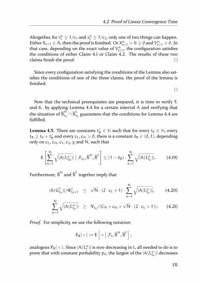
4.2 Proof of Linear Convergence Time
Altogether, for rnt ≥ 1/c1 and snt ≥ 1/c2, only one of two things can happen.
EitherXt+1 ∈ A, then the proof is finished. OrXnt+1 > b ≥ 0 andVnt+1 > 0. Inthat case, depending on the exact value of Vnt+1, the configuration satisfies
the conditions of either Claim 4.1 or Claim 4.2. The results of these two
claims finish the proof.
Since every configuration satisfying the conditions of the Lemma also sat-
isfies the conditions of one of the three claims, the proof of the lemma is
finished.
Now that the technical prerequisites are prepared, it is time to verify 5.
and 6. by applying Lemma 4.4 for a certain interval A and verifying that
the situation of BHt0∩ BLt0 guarantees that the conditions for Lemma 4.4 are
fulfilled.
Lemma 4.5. There are constants t ′R ∈ N such that for every t0 ∈ N, every
tR ≥ t0 + t ′R and every cL, cH > 0, there is a constant δR ∈ (0, 1), dependingonly on cL, cH, c1, c2, χ and N, such that
E
[N∑n=1
√|A(LntR)|
∣∣ Ft0 , BH, BL]≤ (1− δR) ·
N∑n=1
√|A(Lnt0)|. (4.19)
Furthermore, BHand B
Ltogether imply that
|A(G1t0)|/Φ1t0+1
≤√N · (2 · cL + 1) ·
N∑n=1
√|A(Lnt0)|, (4.20)
N∑n=1
√|A(Lnt0)| ≥ Ψt0/(CΨ + cH +
√N · (2 · cL + 1)). (4.21)
Proof. For simplicity, we use the following notation:
ER[ ] := E
[∣∣ Ft, BH, BL] ,
analogous PR( ). Since |A(Lnt )| is non-decreasing in t, all needed to do is to
prove that with constant probability p0, the largest of the |A(Lnt0)| decreases
131

4. Convergence of 1-dimensional PSO
by at least a constant factor of 1 − δ0 with δ0 ∈ (0, 1) within t ′R steps. From
there, it follows that
ER
[N∑n=1
√|A(LntR)|
]≤
N∑n=1
√|A(Lnt0)|− p0 · (1−
√1− δ0) ·max
n
√|A(Lnt0)|
≤ (1− p0 · (1−√1− δ0)/N) ·
N∑n=1
|A(Lnt0)|.
Since there are many substantially different configurations of the particles
and the attractors, a lot of cases need to be considered. We divide the proof
into two parts.
First, we consider the case when at least some local attractors are much
worse than the global attractor, i. e.,
|A(G1t0)| < 1/(2 ·N) ·N∑n=1
|A(Lnt0)|.
Let n0 be in argmax|A(Lnt0)| | n ≤ N. It follows that |A(G1t0)| < |A(Ln0t0 )|/2.The goal is to prove that with a constant probability, particle n0 can halve
its |A(Ln0t )| within a constant number of steps. Let A∗ be the interval of size|A(Ln0t0 )|/2, such that |A(z)| ≤ |A(Ln0t0 )|/2 for every z ∈ A
∗, i. e.,A∗ consists of
the better half of |A(Ln0t )|. Since |A(G1t0)| < |A(Ln0t0 )|/2, we haveA(G1t0) ⊂ A∗
and therefore A(Gnt0) ⊂ A∗, which leads to supx∈A(Gnt0 )
dist(x,A∗) = 0 and
no lower bound on the potential is needed to apply Lemma 4.4. As an upper
bound, we obtain
|Vnt0 |+ |Gnt0 − Xnt0|+ |Lnt0 − X
nt0|
≤ |Vnt0 |+ |Gnt0 −G1t0|+ |G1t0 − X
nt0|+ |Lnt0 −G
1t0|+ |G1t0 − X
nt0|
≤ 2 · (|Vnt0 |+ |G1t0 − Xnt0|) + 2 · |A(Lnt0)|
≤ 2 · (√|Vnt0 |+
√|G1t0 − X
nt0|)2 + 2 · |A(Lnt0)|
≤ 2 · (cH + 1) · |A(Lnt0)| = 4 · (cH + 1) · |A∗|.
With Lemma 4.4, we obtain a lower bound of const(cH, c1, c2, χ) for hittingA∗ within the following t ′R := 3 steps. That finishes the first case.
In the second case, we consider the situation when
|A(G1t0)| ≥ 1/(2 ·N) ·N∑n=1
|A(Lnt0)|.
132

4.2 Proof of Linear Convergence Time
In that situation, it will turn out that the particles improve the global attrac-
tor, such that |A(G)| decreases by at least a constant factor. This implies that
also
∑Nn=1
√|A(Ln)| decreases by a constant factor. While the upper bound
on the potential implies a constant probability for improving the attractors
at all, an additional lower bound on the potential is necessary to ensure that
the improvement is significant. If
∑Nn=1 Y
nt0≤√N · |A(Gnt0)|, it follows that
|A(G1t0)|∑Nn=1 Y
nt0
≤ cL ·N∑n=1
(Ynt0 +√
|A(Lnt0)|) ≤ cL · (√N+
√2 ·N) ·
√|A(G1t0)|
and therefore
N∑n=1
(Ynt0)2 ≥ 1
N·
(N∑n=1
Ynt0
)2≥
|A(G1t0)|
c2L · (1+√2)2 ·N2
.
Altogether, it follows that there is at least one particle n with
|Vnt0 |+ |G1t0 − Xnt0| ≥ (Ynt0)
2 ≥ 1
N·N∑n=1
(Ynt0)2 ≥
|A(G1t0)|
max1, c2L · (1+√2)2 ·N2
.
Let n0 be the first particle with
|Vn0t0 |+ |G1t0 − Xn0t0|+ |Ln0t0 − Xn0t0 | ≥
|A(G1t0)|
maxN2, c2L · (1+√2)2 ·N2, 2(c1 + c2)
.
Before examining the possible improvements made by particle n0, we need
to check by which amount its potential could be decreased during the steps
of the firstn0−1 particles. Imagine that particlen0 has a local attractor equal
to its current position and a velocity close to 0, so all of its potential comes
from the distance to the global attractor, which can be decreased during the
steps of the other particles. I. e., if Gn0t0 ≈ Xn0t0, then the potential of particle
n0 is gone and there is no hope for a significant improvement during its
step. However, if G1t0 and Xn0t0 have the same sign, then G1t0 is already the
closest point to Xn0t0 from the whole interval A(G1t0), so any update of the
global attractor increases the distance. If on the other hand G1t0 and Xn0t0have different signs, any improvement of the global attractor does indeed
decrease the distance |G1t0−Xn0t0| but, since for every particle n < n0 we have
|Vnt0 |+ |G1t0 − Xnt0|+ |Lnt0 − X
nt0| < |A(G1t0)|/(2 · c1 + 2 · c2),
133

4. Convergence of 1-dimensional PSO
decreasing the distance too much is not possible without intermediate up-
dates of the global attractor which reduce |A(G)| considerably. More pre-
cisely: If sign(G1t0) = − sign(Xn0t0 ), then for any particle n < n0, we have
sign(Xnt0) = − sign(Xn0t0 ), i. e., G1t0
is between Xnt0 and Xn0t0 , because other-
wise, we would have
|Vnt0 |+ |G1t0 − Xnt0|+ |Lnt0 − X
nt0| ≥ |G1t0 − X
nt0| ≥ |A(G1t0)|,
a contradiction.
Additionally, if
|A(Gn0t0 )| ≥ |A(G1t0)| · (1− 1/(4c1 + 4c2)),
then there is an interval I of length
|A(Gn0t0 )| ≥ |A(G1t0)| · (1− 1/(2c1 + 2c2))
between particle n0 and all previous particles, that is not visited by any par-
ticle n < n0. Now let n be the first particle to jump over I, i. e.,
|Gnt0 −G1t0| ≤ |A(G1t0)|/(2c1 + 2c2)
and
|Gn+1t0−Gnt0 | ≥ |A(G1t0)| · (1− 1/(2c1 + 2c2)).
For the maximal improvement |Gn+1t0−Gnt0 | of the global attractor during the
step of particle n, that means
|Gn+1t0−Gnt0 | ≤ χ · |V
nt0|+ c1 · |Lnt0 − X
nt0|+ (c2 − 1) · |Gnt0 − X
nt0|
≤ χ · |Vnt0 |+ c1 · |Lnt0− Xnt0 |+ (c2 − 1) · |G1t0 − X
nt0|+ (c2 − 1) · |Gnt0 −G
1t0|
≤ (c1 + c2) · (|Vnt0 |+ |G1t0 − Xnt0|+ |Lnt0 − X
nt0|) + (c2 − 1) · |Gnt0 −G
1t0|
≤ (c1 + c2) · |A(G1t0)|/(4c1 + 4c2) + (c2 − 1) · |A(G1t0)|/(2c1 + 2c2)≤ 3/4 · |A(G1t0)|< |A(G1t0)| · (1− 1/(2c1 + 2c2)).
That concludes the contradiction. In summary, we have shown that one of
the following cases holds:
• |A(Gn0t0 )| < |A(G1t0)| ·(1−1/(2c1+2c2)) (before particle n0’s step, some
other particle has hit interval I),
134

4.2 Proof of Linear Convergence Time
• |Gn0t0 − Xn0t0 | ≥ |A(G1t0)| · (1 − 1/(2c1 + 2c2)) (right before the step of
particle n0, I is still between its position and the global attractor),
• |Gn0t0 − Xn0t0 | ≥ |G1t0 − Xn0t0| (if sign(G1t0) = sign(Xn0t0 )).
In the first case, there is nothing left to prove, and in the second and the
third case, we have
|Vn0t0 |+ |Gn0t0 − Xn0t0 |+ |Ln0t0 − Xn0t0 |
≥|A(G1t0)|
maxN2, c2L · (1+√2)2 ·N2, 2 · c1 + 2 · c2
=|A(G1t0)|
const
For A(G1t0) =: [a, b], choose
A∗ :=
[min
a+
|A(G1t0)|
const · dL, 0
, max
b−
|A(G1t0)|
const · dL, 0
],
where dL denotes the constant from Lemma 4.4. I. e., A∗ is obtained from
A(G1t0) by leaving out an area of size |A(G1t0)|/(const · dL) at each boundary.
Since that way 0might be excluded fromA∗, 0 and the points in between are
added again. Note that the construction makes sure that after hitting A∗,the area that can be entered by the global attractor has size at most |A(G1t0)| ·(1 − 1/(const · dL)) and that the lower bound as demanded by Lemma 4.4
holds.
Since |Gn0t0 −G1t0 | ≤ |A(G1t0)|, the upper bound of
|Vn0t0 |+ |Gn0t0 − Xn0t0 |+ |Ln0t0 − Xn0t0 | ≤ cH · |A(Lnt0)|+ |A(G1t0)|
≤ (4 ·N · cH + 1) · |A(G1t0)| ≤const · (4 ·N · cH + 1)
const− 2· |A∗|.
holds. Lemma 4.4 guarantees a hitting probability, which is bounded from
below by a constant const(cH, N, c1, c2, χ). That finishes the second case and
therefore the proof of (4.19).
135

4. Convergence of 1-dimensional PSO
For the proof of (4.20), we use that
∑Nn=1 Y
nt0≥∑Nn=1
√|A(Lnt0)| implies
that
|A(G1t0)|
Φ1t0+1≤√N · |A(G1t0)|∑N
n=1 Ynt0
≤
√N ·(∑N
n=1
√|A(Lnt0)|
)2∑Nn=1
√|A(Lnt0)|
=√N ·
N∑n=1
√|A(Lnt0)|.
On the other hand, if
∑Nn=1 Y
nt0≤∑Nn=1
√|A(Lnt0)|, we have
|A(G1t0)|
Φ1t0+1≤√N · |A(G1t0)|∑N
n=1 Ynt0
≤√N · cL ·
N∑n=1
(Ynt0 +√|A(Lnt0)|)
≤ 2 ·√N · cL ·
N∑n=1
√|A(Lnt0)|.
That proves (4.20). Finally, we have that
Ψt0 = CΨ ·N∑n=1
√|A(Lnt0)|+
N∑n=1
(√|Vnt0 |+
√|G1t0 − X
nt |
)+
|A(G1t0)|
Φ1t0+1
≤ CΨ ·N∑n=1
√|A(Lnt0)|+ cH ·
N∑n=1
√|A(Lnt0)|
+√N · (2 · cL + 1) ·
N∑n=1
√|A(Lnt0)|
≤ (CΨ + cH +√N · (2 · cL + 1)) ·
N∑n=1
√|A(Lnt0)|.
Statement (4.21) follows immediately.
136

4.2 Proof of Linear Convergence Time
4.2.3 Putting things together
In this section, we combine the technical results from the previous sections
to verify the drift condition of Theorem 3.7 for the concrete choice of a dis-
tance measure Ψt as stated in Definition 4.5.
Lemma 4.6. There are constants tmax ∈ N and δ ∈ (0, 1), such that for
every t ∈ N, there is an Ft-measurable, N-valued random variable σ(t) with
t < σ(t) < t+ tmax almost surely, such that
1Ψt>0 · E[Ψσ(t)∣∣ Ft] ≤ 1Ψt>0 · Ψt · (1− δ).
Proof. For t ∈ N, we consider three cases. The first case is the one of Lemma
4.2, i. e., when
N∑n=1
Ynt ≥ cHN∑n=1
√|A(Lnt )|
for some cH ≥ c ′H to be fixed later. In that case, we set σ(t) := t+ t ′H with t ′Has in Lemma 4.2 and obtain
E[Ψσ(t)∣∣ Ft] = CΨ · N∑
n=1
√|A(Ln
t+t ′H)|+
N∑n=1
Ynt+t ′H+
|A(G1t+t ′H
)|
Φ1t+t ′H+1
(4.3),(4.11)
≤ CΨ ·N∑n=1
√|A(Lnt )|+ (1− δH) ·
N∑n=1
Ynt + Ct ′HL ·
|A(G1t)|
Φ1t+1
= Ψt − δH ·N∑n=1
Ynt + (Ct ′HL − 1) · |A(G
1t)|
Φ1t+1
(4.4),(4.5)
≤ Ψt −δH · Ψt
1+ (CΨ + constH)/cH+ (C
t ′HL − 1) · constH · Ψt
cH
=
(1−
cH · δHcH + CΨ + constH
+ (Ct ′HL − 1) · constH
cH
)· Ψt. (4.22)
In the second case, i. e., in the situation of Lemma 4.3, when
|A(G1t)|/( N∑n=1
Ynt
)≥ cL ·
N∑n=1
(Ynt +√|A(Lnt )|),
137

4. Convergence of 1-dimensional PSO
we set σ(t) := σL with σL as in Lemma 4.3 and obtain
E[Ψσ(t)∣∣ Ft] = CΨ · N∑
n=1
√|A(Ln
σ(t))|
+
N∑n=1
(√|Vnσ(t)|+
√|G1σ(t) − X
nσ(t)|)+
|A(G1σ(t))|
Φ1σ(t)
(4.2),(4.12)
≤ CΨ ·N∑n=1
√|A(Lnt )|+ CH ·
N∑n=1
(Ynt +√|A(Lnt )|)
+ (1− δL) ·|A(G1t)|
Φ1t+1
= Ψt + (CH − 1) ·N∑n=1
(Ynt +√|A(Lnt )|) − δL ·
|A(G1t)|
Φ1t+1
(4.13),(4.14)
≤ Ψt + (CH − 1) · constLcL
· Ψt +N∑n=1
√|A(Lnt )|
−δL · Ψt
1+ constL · CΨ/cL
≤ Ψt + (CH − 1) · constLcL
· Ψt +Ψt
CΨ−
δL · Ψt1+ constL · CΨ/cL
=
(1+ (CH − 1) · constL
cL+1
CΨ
−cL · δL
cL + constL · CΨ
)· Ψt.
(4.23)
Finally, in the situation of Lemma 4.5, when
N∑n=1
Ynt < cH
N∑n=1
√|A(Lnt )|
and
|A(G1t)|/( N∑n=1
Ynt
)< cL ·
N∑n=1
(Ynt +
√|A(Lnt )|
),
138
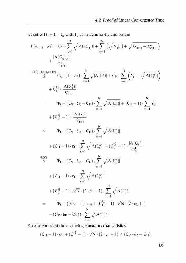
4.2 Proof of Linear Convergence Time
we set σ(t) := t+ t ′R with t ′R as in Lemma 4.5 and obtain
E[Ψσ(t)∣∣ Ft] = CΨ · N∑
n=1
√|A(Ln
σ(t))|+
N∑n=1
(√|Vnσ(t)|+
√|G1σ(t) − X
nσ(t)|
)+
|A(G1σ(t))|
Φ1σ(t)
(4.2),(4.11),(4.19)
≤ CΨ · (1− δR) ·N∑n=1
√|A(Lnt )|+ CH ·
N∑n=1
(Ynt +
√|A(Lnt )|
)+ C
t ′RL ·
|A(G1t)|
Φ1t+1
= Ψt − (CΨ · δR − CH) ·N∑n=1
√|A(Lnt )|+ (CH − 1) ·
N∑n=1
Ynt
+ (Ct ′RL − 1) · |A(G
1t)|
Φ1t+1
≤ Ψt − (CΨ · δR − CH) ·N∑n=1
√|A(Lnt )|
+ (CH − 1) · cH ·N∑n=1
√|A(Lnt )|+ (C
t ′RL − 1) · |A(G
1t)|
Φ1t+1
(4.20)
≤ Ψt − (CΨ · δR − CH) ·N∑n=1
√|A(Lnt )|
+ (CH − 1) · cH ·N∑n=1
√|A(Lnt )|
+ (Ct ′RL − 1) ·
√N · (2 · cL + 1) ·
N∑n=1
√|A(Lnt )|
= Ψt +((CH − 1) · cH + (C
t ′RL − 1) ·
√N · (2 · cL + 1)
− (CΨ · δR − CH))·N∑n=1
√|A(Lnt )|.
For any choice of the occurring constants that satisfies
(CH − 1) · cH + (Ct ′RL − 1) ·
√N · (2 · cL + 1) ≤ (CΨ · δR − CH),
139
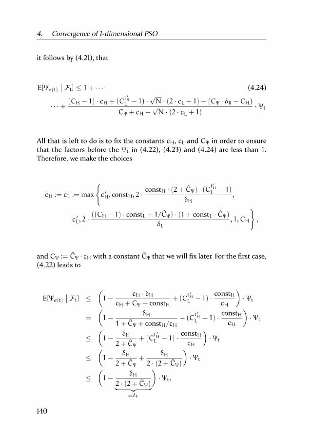
4. Convergence of 1-dimensional PSO
it follows by (4.21), that
E[Ψσ(t)∣∣ Ft] ≤ 1+ · · · (4.24)
· · ·+(CH − 1) · cH + (C
t ′RL − 1) ·
√N · (2 · cL + 1) − (CΨ · δR − CH)
CΨ + cH +√N · (2 · cL + 1)
· Ψt
All that is left to do is to fix the constants cH, cL and CΨ in order to ensure
that the factors before the Ψt in (4.22), (4.23) and (4.24) are less than 1.
Therefore, we make the choices
cH := cL := max
c ′H, constH, 2 ·
constH · (2+ CΨ) · (Ct ′HL − 1)
δH,
c ′L, 2 ·((CH − 1) · constL + 1/CΨ) · (1+ constL · CΨ)
δL, 1, CH
,
and CΨ := CΨ · cH with a constant CΨ that we will fix later. For the first case,
(4.22) leads to
E[Ψσ(t)∣∣ Ft] ≤ (
1−cH · δH
cH + CΨ + constH+ (C
t ′HL − 1) · constH
cH
)· Ψt
=
(1−
δH
1+ CΨ + constH/cH+ (C
t ′HL − 1) · constH
cH
)· Ψt
≤(1−
δH
2+ CΨ+ (C
t ′HL − 1) · constH
cH
)· Ψt
≤(1−
δH
2+ CΨ+
δH
2 · (2+ CΨ)
)· Ψt
≤(1−
δH
2 · (2+ CΨ)︸ ︷︷ ︸=:δ1
)· Ψt.
140
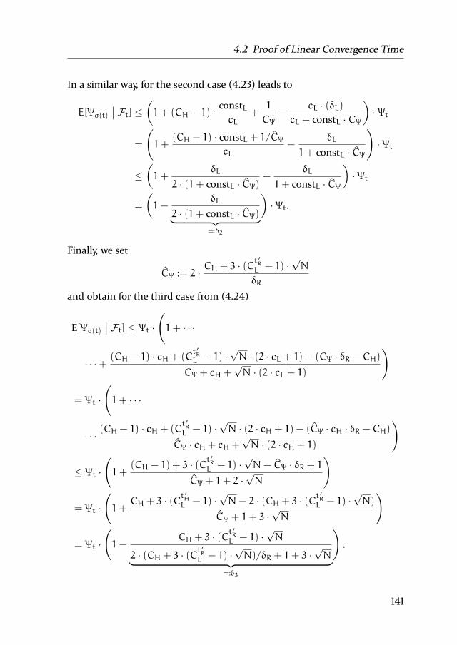
4.2 Proof of Linear Convergence Time
In a similar way, for the second case (4.23) leads to
E[Ψσ(t)∣∣ Ft] ≤ (1+ (CH − 1) · constL
cL+1
CΨ−
cL · (δL)cL + constL · CΨ
)· Ψt
=
(1+
(CH − 1) · constL + 1/CΨcL
−δL
1+ constL · CΨ
)· Ψt
≤(1+
δL
2 · (1+ constL · CΨ)−
δL
1+ constL · CΨ
)· Ψt
=
(1−
δL
2 · (1+ constL · CΨ)︸ ︷︷ ︸=:δ2
)· Ψt.
Finally, we set
CΨ := 2 ·CH + 3 · (Ct
′R
L − 1) ·√N
δR
and obtain for the third case from (4.24)
E[Ψσ(t)∣∣ Ft] ≤ Ψt ·(1+ · · ·
· · ·+(CH − 1) · cH + (C
t ′RL − 1) ·
√N · (2 · cL + 1) − (CΨ · δR − CH)
CΨ + cH +√N · (2 · cL + 1)
)
= Ψt ·
(1+ · · ·
· · ·(CH − 1) · cH + (C
t ′RL − 1) ·
√N · (2 · cH + 1) − (CΨ · cH · δR − CH)
CΨ · cH + cH +√N · (2 · cH + 1)
)
≤ Ψt ·
(1+
(CH − 1) + 3 · (Ct′R
L − 1) ·√N− CΨ · δR + 1
CΨ + 1+ 2 ·√N
)
= Ψt ·
(1+
CH + 3 · (Ct′H
L − 1) ·√N− 2 · (CH + 3 · (Ct
′R
L − 1) ·√N)
CΨ + 1+ 3 ·√N
)
= Ψt ·
(1−
CH + 3 · (Ct′R
L − 1) ·√N
2 · (CH + 3 · (Ct′R
L − 1) ·√N)/δR + 1+ 3 ·
√N︸ ︷︷ ︸
=:δ3
).
141

4. Convergence of 1-dimensional PSO
With δ := minδ1, δ2, δ3 and tmax := maxt ′H, t′L, t′R the proof is finished.
Now, everything is prepared to apply our drift theorem, Theorem 3.7.
Theorem4.2. Let b be the diameter of the search space and assume that the
particles are initialized such that E[∑Nn=1 Y
nt ] ≤ CY ·
√b and E[1/Φ1t+1] ≤ CΦ
for two constants CY , CΦ > 0. This is the case, e. g., when the particles’
positions are initialized independently and uniformly over [−b, b] and if the
velocities have finite expectation. Then there is a constant c, depending only
on the swarm parameters χ, c1, c2 andN, such that the following holds: Let
τ := mint ≥ 0∣∣ Ψt ≤ 2−k. Then we have
E[τ] ≤ const(χ, c1, c2, N, a, CY , CΦ) · (k+ log(b+ 1) + 1).
Proof. We define Zt := 2k ·Ψt. Then, Lemma 4.6 implies that for every t ∈ N
1Zt>1 · E[Zσ(t)∣∣ Ft] ≤ 1Zt>1 · Zt · (1− δ)
for some δ ∈ (0, 1) and some Ft-measurable σ(t) with t ≤ σ(t) ≤ t+ tmax ∈N. Note that Zt ≤ 1⇔ Ψt ≤ 2−k. By Theorem 3.7, it follows that
E[τ∣∣ F0] ≤ tmax · 1Z0>1 · (log(Z0) + 2)/δ
and therefore
E[τ] = E[E[τ∣∣ F0]] ≤ E[tmax·1Z0>1·(ln(Z0)+2)/δ] ≤ tmax·(k·log(E[Ψ0])+2)/δ.
As for the expectation of Ψ right after the initialization, we have
E[Ψ0] = E
[CΨ ·
N∑n=1
√|A(Lnt )|+
N∑n=1
Ynt +|A(G1t)|
Φ1t+1
]≤ CΨ ·N ·
√b+ CY ·
√b+ CΦ · b
≤ (CΨ ·N+ CY + CΦ) ·maxb,√b
and therefore
E[τ] ≤ tmax · (ln(2) · k+ log(CΨ ·N+ CY + CΦ) + log(maxb,√b) + 2)/δ
≤ tmax/δ ·max1, log(CΨ ·N+ CY + CΦ) + 2︸ ︷︷ ︸=:c
·(k+ log(b+ 1) + 1)
That finishes the proof.
142

4.2 Proof of Linear Convergence Time
In order to provide some experimental insight as well, we calculated the
complete measure Ψ with CΨ := 1 for swarms processing the objective func-
tions SPHERE and SPHERE+in the following experiment.
Experiment 4.5. As before, the swarm sizes N = 2 and N = 10 are tested
and the particles are initialized over [−100, 100] for processing SPHERE and
[0, 100] for optimizing SPHERE+. The results can be seen in Figure 4.12.
0 1000 2000 3000 4000 5000 6000 7000 8000 9000 1000010-250
10-200
10-150
10-100
10-50
100
1050
(a)Optimizing SPHERE.
0 1000 2000 3000 4000 5000 6000 7000 8000 9000 1000010-250
10-200
10-150
10-100
10-50
100
1050
(b)Optimizing SPHERE+.
Figure 4.12: Course of optimality measure Ψ while processing objective
function SPHERE and SPHERE+
for swarm sizes N = 2 and
N = 10.
Actually, increasing the swarm size does in the 1-dimensional situation
not increase the speed by which Ψ decreases. The reason for this might be
that the run time consists mostly of the phases when the potential needs to
be decreased, which has to be done by every particle independently of the
others and can therefore not be accelerated by increasing the swarm size.
Therefore, the experiments indicate that the smallestN, for which the swarm
converges towards the optimum at all, might be already the optimal choice
for the swarm size.
143

5. Convergence for MultidimensionalProblems
In the previous chapter, we have demonstrated the power of the bad-events-
technique to analyze the classical particle swarm optimization (PSO) in case
of 1-dimensional objective functions. We studied two bad events, namely the
event of a potential too high and the event of a potential too low to allow a
sufficiently large expected improvement of the global attractor within near
future. We have been shown that without any modification, PSO can heal
itself from encountering any of the two bad events. This implies that the
swarm can find local optima and furthermore, if the objective function is
unimodal, we were able to prove a runtime bound.
As it will turn out soon, we cannot achieve the same results in the more
general D-dimensional case. Here, certain bad events exist from which the
swarm might not be able to heal itself. But still, studying the bad events is
fruitful because the investigations uncover the possible weaknesses of the
swarm and allow for a distinction between ordinary bad events, from which
the particle swarm recovers on its own, and “fatal events” that might indeed
prevent the swarm from finding a local optimum and therefore make inter-
vention necessary.
In the first part of this chapter, we expose the bad events of the D-di-
mensional case and empirically examine them for if they are fatal or not.
Although the complicated interdependencies between different dimensions
prevent a formal run time analysis, we suggest appropriate informal sec-
ondary measures based on the potential and present experimental investi-
gations of these measures during the respective bad events. Afterwards, we
apply a modification to the PSO algorithm, enabling it to heal itself from the
former fatal events. We prove that the resulting method almost surely finds
local optima, similar to the 1-dimensional situation.
Finally, we present experiments using standard double precision numbers
to demonstrate that the examined phenomena are not just artifacts of the
implementation with arbitrary precision numbers, but that they show up
and effect the quality of the solution found even in standard situations.
145

5. Convergence for Multidimensional Problems
5.1 Determining Further Bad Events
There are three essentially different bad events, i. e., three different condi-
tions on the configuration of the swarm, preventing major improvements of
the attractors. These three bad events lead to a very different behavior of the
particle swarm and will be examined in detail during this section.
The first bad event occurs when in at least one dimension d0, the swarm
has a too high potential, such that the probability for updating the attrac-
tor at all is small. I.e., this happens when in dimension d0 the potential is
orders of magnitude larger than the area that would improve the attractors,
while the potential in other dimensions, whose corresponding entries of the
global attractor could be improved, is much smaller than in dimension d0.
Therefore, the overall value of the objective function depends almost only
on the entries in dimensions like d0 with too high potential and it is unlikely
that the swarm updates the global attractor. If this bad event occurs, which
can be seen as the D-dimensional generalization of the bad event BHt from
the previous chapter, the swarm needs to decrease its potential in dimension
d0 to heal itself.
Second and similar to the event BLt from the previous chapter, configura-
tions could occur in which the whole swarm has in every dimension a poten-
tial much smaller than the distance to the next local optimum. In that case,
the desired behavior of the swarm is to accelerate and to charge potential.
Finally, there is a bad event which can only occur if D ≥ 2, namely the
case of very imbalanced potentials. If the potential is very imbalanced, i. e.,
if there is a dimension d0 with a potential much smaller than in the other
dimensions, then the d0’th entry of a position has almost no influence on
the decision whether an attractor gets updated after the next step or not.
If additionally the d0’th entry of the global attractor differs much from the
corresponding entry of the next local optimum, the swarm is unlikely to de-
crease that distance and might behave like in the D − 1-dimensional situa-
tion, optimizing all dimensions except for d0. In order to recover from this
imbalanced state, the swarmmust “turn around the corner”, i. e., the quotient
Φd0t /∑Dd=1Φ
dt must increase.
As it turns out, the swarm can heal itself from the first two bad events
easily, while the third bad eventmight become fatal evenwhen PSOprocesses
the very simple function SPHERE. Therefore, we study the third event in
detail to find a modification that allows the swarm to recover from it.
146

5.1 Determining Further Bad Events
Throughout this section, we assume that the objective function has the
form f(x) = xt · A · x with a positive-definite matrix A. While this may
sound very restrictive, every analytic function g can near a simple local op-
timum, i. e., a local optimum where all second derivatives are non-zero, be
approximated by such a function f, where A is the Jacobi-matrix of g.
5.1.1 High Potential in at least one Dimension: A Bad Event
If the potential in a certain dimension d is too large, the behavior of the
swarm is very similar to the 1-dimensional case. Let
πd(A) := xd ∈ R | ∃x1, . . . , xd−1, xd+1, . . . , xD ∈ R : (x1, . . . , xD) ∈ A
denote the projection of some set A ⊂ RD on the d-axis. Then, a necessary
condition for an improvement of the local attractor of particlen is thatXn,dt ∈πd(ALnt ). Now, we can formulate the bad event of a too high potential as
BHt :=
∃d ∈ 1, . . . , D :
N∑n=1
Yn,dt ≥ cH ·N∑n=1
√|πd(ALnt )|
with
Yn,dt =√
|Vn,dt |+√|G1,dt − Xn,dt |
as an alternative measure for the potential, similar to the 1-dimension case
(Definition 3.9). A graphical representation of this bad event BHt is given in
Figure 5.1.
Similar to the 1-dimensional case, the Yn,dt can serve as a secondary mea-
sure for this event, in terms:
ΨHt :=
D∑d=1
N∑n=1
Yn,dt .
In order to examine how the particle swarm performs when confronted
with such a configuration, Experiment 4.2 from the previous chapter is re-
peated with more than 1 dimension. Since in [LW11] the function SPHERE+
is only defined as a 1-dimensional function, we define its D-dimensional
generalization as
SPHERE+((x1, . . . , xD)) :=
SPHERE((x1, . . . , xD)), if mind=1,...,D xd ≥ 0,∞, otherwise,
147

5. Convergence for Multidimensional Problems
dimension 2
dim
ensi
on 1
particle
global attractor
velocity
Figure 5.1: Dimension 1 has a too high potential and voids possible improve-
ments in dimension 2.
i. e., SPHERE+(x) is identical to SPHERE(x) if all the coordinate entries of x
are non-negative. Otherwise, SPHERE+(x) is infinite. Figure 5.2 shows the
comparison of the functions SPHERE and SPHERE+. Similar as before, SPHERE
represents the type of function which is perfectly symmetric, i. e., the area
A(x) of points as least as good as some fixed point x is always a ball around
the optimum, while SPHERE+is as asymmetric as possible with the optimum
in a corner of A(x).
Experiment 5.1. For the experiment, we set the search space dimension to
10 and use swarm sizes N = 2 and N = 10 for each of the two functions.
We initialize the particles’ positions in [−10−100, 10−100] in order to guar-
antee that the attractors are close to the optimum. In combination with
148
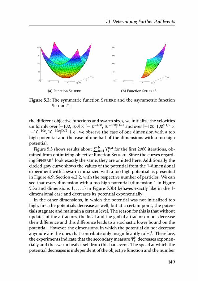
5.1 Determining Further Bad Events
-10 -5 0 5 10 -10
0
10
0
50
100
150
200
(a) Function SPHERE.
-10 -5 0 5 10 -10
0
10
0
50
100
150
200
(b) Function SPHERE+.
Figure 5.2: The symmetric function SPHERE and the asymmetric function
SPHERE+.
the different objective functions and swarm sizes, we initialize the velocities
uniformly over [−100, 100]× [−10−100, 10−100]D−1and over [−100, 100]D/2 ×
[−10−100, 10−100]D/2, i. e., we observe the case of one dimension with a too
high potential and the case of one half of the dimensions with a too high
potential.
Figure 5.3 shows results about
∑Nn=1 Y
n,dt for the first 2000 iterations, ob-
tained from optimizing objective function SPHERE. Since the curves regard-
ing SPHERE+look exactly the same, they are omitted here. Additionally, the
circled gray curve shows the values of the potential from the 1-dimensional
experiment with a swarm initialized with a too high potential as presented
in Figure 4.9, Section 4.2.2, with the respective number of particles. We can
see that every dimension with a too high potential (dimension 1 in Figure
5.3a and dimensions 1, . . . , 5 in Figure 5.3b) behaves exactly like in the 1-
dimensional case and decreases its potential exponentially.
In the other dimensions, in which the potential was not initialized too
high, first the potentials decrease as well, but at a certain point, the poten-
tials stagnate andmaintain a certain level. The reason for this is that without
updates of the attractors, the local and the global attractor do not decrease
their difference and this difference leads to a stochastic lower bound on the
potential. However, the dimensions, in which the potential do not decrease
anymore are the ones that contribute only insignificantly to ΨHt . Therefore,
the experiments indicate that the secondarymeasureΨHt decreases exponen-
tially and the swarm heals itself from this bad event. The speed at which the
potential decreases is independent of the objective function and the number
149

5. Convergence for Multidimensional Problems
of dimensions and depends only a little on the swarm size. That is because
during this bad event, the updates of the local and global attractors are rare
and every dimension behaves like an independent copy of the 1-dimensional
process in the same situation.
0 200 400 600 800 1000 1200 1400 1600 1800 200010-60
10-50
10-40
10-30
10-20
10-10
100
1010
dimension 1
curve of 1-dimensionalexperiment
0 200 400 600 800 1000 1200 1400 1600 1800 200010-50.05
10-50
10-49.95
10-49.9
10-49.85
10-49.8
10-49.75
10-49.7
10-49.65
10-49.6
10-49.55
dimension 2
dimension 3
dimension 4
dimension 5
dimension 6
dimension 7
dimension 8
dimension 9
dimension 10
dimensions 2,...,10
(a) Potential of N = 2 particles processing SPHERE after being initialized with a too high
potential in dimension 1.
0 200 400 600 800 1000 1200 1400 1600 1800 200010-50
10-40
10-30
10-20
10-10
100
1010
curve of 1-dimensionalexperiment
0 200 400 600 800 1000 1200 1400 1600 1800 200010-49.02
10-49
10-48.98
10-48.96
10-48.94
10-48.92
10-48.9
10-48.88
10-48.86
dimension 6
dimension 7
dimension 8
dimension 9
dimension 10
dimensions 1,...,5
dimensions 6,...,10
(b) Potential of N = 10 particles processing SPHERE after being initialized with a too high
potential in dimensions 1, . . . , 5.
Figure 5.3: Particle swarm suffering from too high potentials while process-
ing 10-dimensional objective function SPHERE with N = 2 or
N = 10 particles, initialized with 1 or D/2 dimensions with too
high potential. For comparison, the curve of a 1-dimensional
PSO with a too high potential is added.
Indeed, the self-healing capacity of the particle swarm from the bad event
BHt can be proved, with a proof that is similar to the proof of Lemma 4.2 for
1-dimensional case.
150
5.1 Determining Further Bad Events
Lemma 5.1. There are constants t ′H ∈ N, c ′H > 0, CH > 0, δH ∈ (0, 1) andconstH, depending only on c1, c2, χ andN, such that for every t0 ∈ N, every
tH ≥ t0 + t ′H and every cH > c′H, we have
E
[N∑n=1
Yn,dtH
∣∣ Ft0]≤ CH ·
(N∑n=1
Yn,dt0 +
N∑n=1
√|A(Lnt0)|
), (5.1)
E
[N∑n=1
Yn,dtH
∣∣ Ft0 , BHt0]≤ (1− δH) ·
N∑n=1
Yn,dt0 , (5.2)
(5.3)
Proof. The proof is exactly the same as the proof of (4.2) and (4.3) of Lemma
4.2 in the previous chapter. Here, πd(ALnt ) plays the role of ALnt in the 1-
dimensional case. Note that the proof of Lemma 4.2 only makes use of the
fact that the local attractor is not updated outside of ALnt , which is also true
for its d’th coordinate outside of πd(ALnt ) in theD-dimensional case. Lemma
4.2 did not use the fact that inside of ALnt , the attractor actually is updated,
which was the case in the 1-dimensional situation but is not necessarily true
in the D-dimensional case because if Xn,dt ∈ πd(ALnt ), then it still depends
on the other entries of Xnt , whether or not the attractor is updated.
In particular, the conditions on the swarm parameters for which the par-
ticle swarm can heal itself from the bad event BHt are the same as in the
1-dimensional case, i. e., the same as specified in Theorem 3.11.
5.1.2 Low Potential in every Dimension: A Bad Event
Another bad event occurs when the potential of the swarm is too small in
every single dimension, such that only search points very close to the global
attractor are visited and therefore every possible improvement is insignif-
icant. In order to recover from such a configuration, the swarm needs to
accelerate and to charge potential until its updates become again significant.
This event could be formulated as
BLt :=
∀d ∈ 1, . . . , D : Φdt
√|G1,dt |
.
Figure 5.4 provides a graphical representation of the bad event BHt .
151

5. Convergence for Multidimensional Problems
dimension d1
dim
ensi
on d
0
particle
global attractor
velocity
Figure 5.4: All dimensions have a potential too small tomake significant im-
provements of the global attractor
A possible secondary measure for this event could be
∑Dd=1 |G
1,dt |∑D
d=1Φdt
.
To study the behavior of the swarm in such a situation, we use the objective
function INCLINEDPLANE, defined as
INCLINEDPLANE(~x) = −
D∑d=1
xd.
152
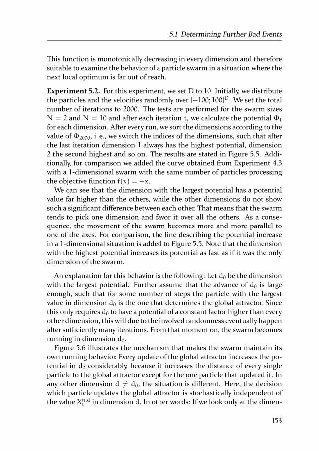
5.1 Determining Further Bad Events
This function is monotonically decreasing in every dimension and therefore
suitable to examine the behavior of a particle swarm in a situation where the
next local optimum is far out of reach.
Experiment 5.2. For this experiment, we setD to 10. Initially, we distribute
the particles and the velocities randomly over [−100; 100]D. We set the total
number of iterations to 2000. The tests are performed for the swarm sizes
N = 2 and N = 10 and after each iteration t, we calculate the potential Φtfor each dimension. After every run, we sort the dimensions according to the
value of Φ2000, i. e., we switch the indices of the dimensions, such that after
the last iteration dimension 1 always has the highest potential, dimension
2 the second highest and so on. The results are stated in Figure 5.5. Addi-
tionally, for comparison we added the curve obtained from Experiment 4.3
with a 1-dimensional swarm with the same number of particles processing
the objective function f(x) = −x.We can see that the dimension with the largest potential has a potential
value far higher than the others, while the other dimensions do not show
such a significant difference between each other. That means that the swarm
tends to pick one dimension and favor it over all the others. As a conse-
quence, the movement of the swarm becomes more and more parallel to
one of the axes. For comparison, the line describing the potential increase
in a 1-dimensional situation is added to Figure 5.5. Note that the dimension
with the highest potential increases its potential as fast as if it was the only
dimension of the swarm.
An explanation for this behavior is the following: Let d0 be the dimension
with the largest potential. Further assume that the advance of d0 is large
enough, such that for some number of steps the particle with the largest
value in dimension d0 is the one that determines the global attractor. Since
this only requires d0 to have a potential of a constant factor higher than every
other dimension, this will due to the involved randomness eventually happen
after sufficientlymany iterations. From thatmoment on, the swarmbecomes
running in dimension d0.
Figure 5.6 illustrates the mechanism that makes the swarm maintain its
own running behavior. Every update of the global attractor increases the po-
tential in d0 considerably, because it increases the distance of every single
particle to the global attractor except for the one particle that updated it. In
any other dimension d 6= d0, the situation is different. Here, the decision
which particle updates the global attractor is stochastically independent of
the value Xn,dt in dimension d. In other words: If we look only at the dimen-
153

5. Convergence for Multidimensional Problems
0 200 400 600 800 1000 1200 1400 1600 1800 2000100
1010
1020
1030
1040
1050
1060
dimension 10
dimension 9
dimension 8
dimension 7
dimension 6
dimension 5
dimension 4
dimension 3
dimension 2
dimension 1
curve of 1-dimensionalexperiment
(a) Swarm size N = 2
0 200 400 600 800 1000 1200 1400 1600 1800 2000100
1050
10100
10150
10200
10250
10300
10350
10400
10450
10500
dimension 10
dimension 9
dimension 8
dimension 7
dimension 6
dimension 5
dimension 4
dimension 3
dimension 2
dimension 1
curve of 1-dimensionalexperiment
(b) Swarm size N = 10
Figure 5.5: Growth of potential when processing objective function IN-
CLINEDPLANE with swarm size
(a) N = 2,(b) N = 10.
sion d, the global attractor is chosen uniformly at random from the set of all
particles’ positions. As a consequence, after some iterations, the d0’th coor-
dinate of the velocity becomes positive for every particle, so the attraction
towards the global attractor always goes into the same direction as the veloc-
ity, while in the remaining dimensions, the velocities may as well point away
from the global attractor, meaning that the particles will be slowed down by
the force of attraction.
So, roughly speaking, most of the time the global attractor is somewhere
in the middle of the different Xn,dt values for the different particles, giving
less potential increase than in dimension d0 where it has a border position.
That means that the balanced situation is not stable in a sense that after
the imbalance of the potentials in the different dimensions has reached a
certain critical value, it will grow unboundedly. From that point on, the de-
cision about attractor updates depends almost only on dimension d0, there-
fore from the perspective of this dimension, the swarm behaves like in the
1-dimensional case.
These considerations indicate that indeed the swarm heals itself from the
bad event BLt by choosing one dimension d0 and becoming running in di-
rection d0 until the objective function is no longer decreasing in that direc-
tion. In particular, since it is always exactly one dimension which is chosen,
the conditions to the swarm parameters, that allow the swarm to actually
154

5.1 Determining Further Bad Events
particle
global attractor
velocity
Figure 5.6: Particles running in direction d0. In dimension d0, the differ-
ences between the coordinate of the particle and the global at-
tractor is on average higher than in dimension d1. The velocities
of dimension d0 point in the direction of the global attractor.
increase its potential while running, are again exactly the same as in the 1-
dimensional case.
Unfortunately, a new problem arises. When the swarm stops running, the
potential in dimension d0 is of the same order as the distance between the
swarm and the d0’th coordinate of the optimum, while every other dimen-
sion has a potential much smaller than d0. Therefore, the swarm continues
improving the global attractor in dimension d0 while ignoring its other com-
ponents. However, as soon as the room for improvements in dimension d0 is
sufficiently much smaller than in some other dimension, possible improve-
ments of the other dimensions are dominated by the “random noise” of di-
mension d0, i. e., if an attractor is updated or not depends still much more
on the respective entries in dimension d0 than on possible improvements of
other dimensions. Therefore, the swarm is again not in a situation to make
significant progress. This leads to the third bad event, namely the event of
imbalanced potentials.
155
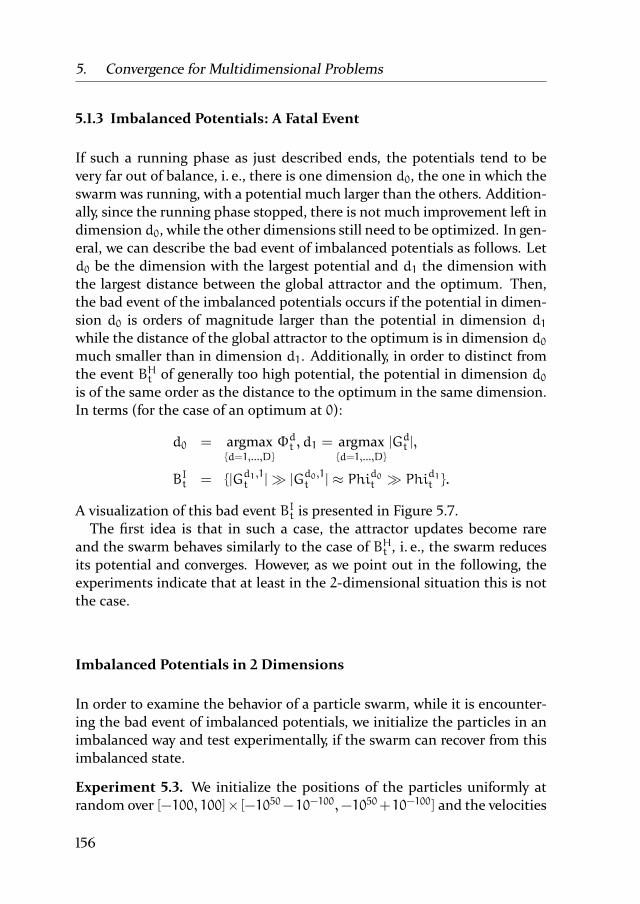
5. Convergence for Multidimensional Problems
5.1.3 Imbalanced Potentials: A Fatal Event
If such a running phase as just described ends, the potentials tend to be
very far out of balance, i. e., there is one dimension d0, the one in which the
swarm was running, with a potential much larger than the others. Addition-
ally, since the running phase stopped, there is not much improvement left in
dimension d0, while the other dimensions still need to be optimized. In gen-
eral, we can describe the bad event of imbalanced potentials as follows. Let
d0 be the dimension with the largest potential and d1 the dimension with
the largest distance between the global attractor and the optimum. Then,
the bad event of the imbalanced potentials occurs if the potential in dimen-
sion d0 is orders of magnitude larger than the potential in dimension d1while the distance of the global attractor to the optimum is in dimension d0much smaller than in dimension d1. Additionally, in order to distinct from
the event BHt of generally too high potential, the potential in dimension d0is of the same order as the distance to the optimum in the same dimension.
In terms (for the case of an optimum at 0):
d0 = argmax
d=1,...,D
Φdt , d1 = argmax
d=1,...,D
|Gdt |,
BIt = |Gd1,1t | |Gd0,1t | ≈ Phid0t Phid1t .
A visualization of this bad event BIt is presented in Figure 5.7.
The first idea is that in such a case, the attractor updates become rare
and the swarm behaves similarly to the case of BHt , i. e., the swarm reduces
its potential and converges. However, as we point out in the following, the
experiments indicate that at least in the 2-dimensional situation this is not
the case.
Imbalanced Potentials in 2 Dimensions
In order to examine the behavior of a particle swarm, while it is encounter-
ing the bad event of imbalanced potentials, we initialize the particles in an
imbalanced way and test experimentally, if the swarm can recover from this
imbalanced state.
Experiment 5.3. We initialize the positions of the particles uniformly at
random over [−100, 100]× [−1050−10−100,−1050+10−100] and the velocities
156

5.1 Determining Further Bad Events
dimension d1
dim
ensi
on d
0
particle
global attractor
velocity
Figure 5.7: Imbalanced Potentials: The swarm is in dimension d1 much far-
ther away from the optimum than in dimension d0, while the
potential of dimension d0 is much larger than the potential of
dimension d1.
over [−100, 100] × [−10−100, 10−100], such that the second dimension has a
much larger distance to the optimum, but a much lower potential than di-
mension 1. In particular, the potential in dimension 1 is sufficient to reach
the optimum, while the potential in dimension 2 is not. We choose two ob-
jective functions, namely SPHERE (Figure 5.2a) and SCHWEFEL ([SHL+05],
Figure 5.8), defined as
SCHWEFEL(~x) =D∑d=1
( d∑d ′=1
xd ′
)2.
157

5. Convergence for Multidimensional Problems
We test PSO with swarm sizes N = 2 and N = 10.
-10-5
05
10 -10
0
10
0
100
200
300
400
500
Figure 5.8:Objective function SCHWEFEL.
The results regarding objective function SPHERE can be seen in Figure 5.9.
Figure 5.9a shows the curve of the potentials in both dimensions for swarm
size N = 2, while Figure 5.9b shows the courses of the absolute value of the
according entry of the global attractors.
We see that during the first ≈ 900 iterations, only the first entry of the
global attractor is improved, while the second entry stays about constant.
Meanwhile, the potentials of both dimensions decrease. For comparison, a
part of the line obtained in Experiment 4.2, where a 1-dimensional swarm
was initialized with a too high potential, is added (“stagnating dimension”
in Figure 5.9a). Note that here two different measures of potential are com-
pared, but as stated before, they differ by at most a constant factor and are in
the current situation both exponentially decreasing, therefore the compar-
ison is still meaningful. We see that dimension 1 decreases with the same
speed as the potential in Experiment 4.2, while dimension 2 decreases sig-
nificantly slower.
158

5.1 Determining Further Bad Events
0 500 1000 1500 2000 2500 3000 3500 4000 4500 500010-60
10-50
10-40
10-30
10-20
10-10
100
1010
1020
1030
dimension 1
dimension 2
running dimension
next to running dimension
stagnating dimension
(a) Potential curve of N = 2 particles ini-tialized with imbalanced potentials.
0 500 1000 1500 2000 2500 3000 3500 4000 4500 500010-40
10-30
10-20
10-10
100
1010
1020
1030
1040
1050
1060
dimension 1
dimension 2
(b) Global attractor getting improved over
time.
0 500 1000 1500 2000 2500 3000 3500 4000 4500 500010-60
10-50
10-40
10-30
10-20
10-10
100
1010
1020
1030
dimension 1
dimension 2
running dimension
next to running dimension
stagnating dimension
(c) Potential curve ofN = 10 particles ini-tialized with imbalanced potentials.
0 500 1000 1500 2000 2500 3000 3500 4000 4500 500010-120
10-100
10-80
10-60
10-40
10-20
100
1020
1040
1060
dimension 1
dimension 2
(d) Global attractor getting improved over
time.
Figure 5.9: Particle swarm recovering from imbalanced potentials while pro-
cessing 2-dimensional objective function SPHERE with N = 2 orN = 10 particles, initialized with a too low potential and a very
high distance to the optimum in dimension 2.
The reason for this is the following: If after one step of a particle, the
new position becomes the new local or even global attractor, depends almost
only on the first dimension’s entry of the respective positions. Therefore, the
first dimension behaves similar to a 1-dimensional PSO and decreases its
potential with the same speed as in the 1-dimensional case. However, since
the process of optimizing dimension 1 yields a certain update frequency for
the attractors, the situation is not the same for dimension 2. In dimension 1,
the distance between the old and the new global attractor at each update is
limited, i. e., the global attractor can only be updated to points that are close
(in relation to Φd0t ) to its previous position and therefore tend to be in the
159

5. Convergence for Multidimensional Problems
middle of the swarm. On the other hand, since the positions of the particles
in dimension 2 have almost no influence on the update probability for the
attractors, the difference between the previous and the new position of the
global attractor after each update are of order (Φ2t)2. Figure 5.10 illustrates
this self-healing effect.
particle
global attractor
velocity
Figure 5.10: Particles optimizing dimension d0 while stagnating in dimen-
sion d1. Updates of attractors depend mostly on the d0’th entry
of the updated position and an attractor update is performed if
this entry is comparatively close to the respective entry of the
global attractor. Therefore, changes in dimension d1 have only
little effect on the updates, but from the perspective of dimen-
sion d1 the attractor updates comewith a certain frequency and
are independent of the positions. If, e. g., the marked particle
moves and updates the global attractor, the distance between
the old and the updated global attractor has muchmore impact
on dimension d1 than on dimension d0.
In summary, we can see PSO in both dimensions as two processes with
different behavior. In dimension 1, a 1-dimensional PSO is run while in di-
160

5.1 Determining Further Bad Events
mension 2, a PSO-like process is run where the decision if after a step an
attractor is updated comes from “outside”, namely from dimension 1, which
causes attractor updates at a certain frequency. Therefore, if the global at-
tractor is updated, then |Gn+1,1t − Xn,1t+1| is much smaller than the (squared)
potential of dimension 1, while |Gn+1,2t −Xn,2t+1| is of order (Ψn,dt )2. So, the pro-
cess describing dimension 2 benefits more from updates than the process of
dimension 1. Therefore, the “amount of imbalance” decreases.
Note the similarity of this effect and the situation when the swarm is run-
ning. If the swarm is running in a certain dimension d0, then in this di-
mension the attractor is always at the border of the area populated by the
particles, while in every other dimensions it is randomly distributed. Since
a global attractor at the border maximizes the sum of the distances between
the particles and the global attractor, dimension d0 is able to increase its
potential faster. If on the other hand dimension d0 is converging, then the
global attractor is in dimension d0 in the middle of the swarm and therefore
minimizing the distances between the particles and the global attractors,
while in every other dimension it is again randomly distributed. Therefore,
the potential of dimension d0 shrinks faster than the potential of the other
dimensions.
Although this effect is apparently not strong enough to cause an increase
of the potential in dimension 2, at least it slows down the decrease ofΦ2t and
therefore causes an increase of Φ2t/Φ1t . Therefore, after some iterations, the
conditionΦ1t Φ2t is violated and the swarm has healed itself from the bad
event BIt.
Finally, at iteration ≈ 900, the swarm has fully recovered from the imbal-
anced potentials. Note that this self-healing does not necessarily require the
potential in dimension 2 to overcome the potential of dimension 1. Since
the gradient of the function is different in different regions, the remaining
distance still allows for dimension 2 to have significant impact on the up-
dates of the attractors. In this situation, dimension 1 has a potential too low
in comparison with the distance to the optimum. Dimension 2 is generally
insignificant because it does not contribute much to the decision about at-
tractor updates. Next, the swarm becomes running in dimension 2, i. e., the
potential of dimension 2 increases faster than the potential in dimension 1.
For comparison, shifted (but not scaled) versions of the curves fromExper-
iment 5.2 are added to Figure 5.9a, where the swarmwas run on the objective
function INCLINEDPLANE in order to simulate the case of a too low potential
in every dimension. In Experiment 5.2, one particular dimension, which was
afterwards renamed as “dimension 1”, was randomly chosen by the process,
161

5. Convergence for Multidimensional Problems
in which the potential increased much faster than in the others, while the
potentials of the remaining dimensions increased about equally. The curve
“running dimension” refers to this special dimension 1 of Experiment 5.2
and the curve “next to running dimension” to dimension 10 of Experiment
5.2. We can see that indeed the increases of the different potentials for both
situations behave quite similar.
Note that during this running phase, since the potential in dimension 1
increases and the attractor updates depend almost only on dimension 2, the
first coordinate of the global attractor gets worse while its second coordinate
improves, such that there is an overall improvement of its objective function
value. In Figure 5.9b, we can see |G1,1t | increasing. For an explanation why
the improvement of |G1,2t | is at the beginning not visible, one has to recall
that the axes are logarithmically scaled. The values |G1,1t | and |G1,2t | are a
factor of ≈ 1080 away from each other, while in the objective function, their
squares are summed. Therefore decreasing |G1,2t | by, e. g., a factor of 0.999,
which would not be visible in the figure, improves the global attractor, even if
it comes with an |G1,1t | increased by, e. g., a factor of 1040, which would indeed
be clearly visible.
In Figure 5.9c and Figure 5.9d, we present the respective curves for a swarm
withN = 10 particles. We see that the behavior is essentially the same as in
the case of N = 2 particles. During the first phase, the potential of dimen-
sion 2 decreases slower than with only N = 2 particles, which results in a
shorter time necessary for overcoming the imbalance. As seen before, also
the increase of potential during the running phase happens faster with more
particles, therefore the second phase is again shorter.
The corresponding results regarding objective function SCHWEFEL are pre-
sented in Figure 5.11.
There is a crucial difference between the objective functions SPHERE and
SCHWEFEL. The function SPHERE is separable, which in particular means
that for every constant ~c = (c1, . . . , cD) ∈ RD−1, we have
argmin
x∈RSPHERE((x, c1, . . . , cD)) = 0.
The same is not true for the function SCHWEFEL. Formally, for a function
f(~x) = ~xt ·A ·~x with a positive definite matrix A ∈ RD×D, a position ~z ∈ RD
and a dimension d ∈ 1, . . . , D, we define
y∗(~z, d) := argmin
x∈Rf((z1, . . . , zd−1, x, zd+1, . . . , zD)) = 0
162

5.1 Determining Further Bad Events
0 500 1000 1500 2000 2500 3000 3500 4000 4500 500010-60
10-50
10-40
10-30
10-20
10-10
100
1010
1020
1030
dimension 1
dimension 2
running dimension
next to running dimension
stagnating dimension
(a) Potential curve of N = 2 particles ini-tialized with imbalanced potentials.
0 500 1000 1500 2000 2500 3000 3500 4000 4500 5000100
1010
1020
1030
1040
1050
1060
dimension 1
dimension 2
(b) Global attractor getting improved over
time.
0 500 1000 1500 2000 2500 3000 3500 4000 4500 500010-60
10-50
10-40
10-30
10-20
10-10
100
1010
1020
1030
dimension 1
dimension 2
running dimension
next to running dimension
stagnating dimension
(c) Potential curve ofN = 10 particles ini-tialized with imbalanced potentials.
0 500 1000 1500 2000 2500 3000 3500 4000 4500 500010-60
10-40
10-20
100
1020
1040
1060
dimension 1
dimension 2
(d) Global attractor getting improved over
time.
Figure 5.11: Particle swarm recovering from imbalanced potentials while
processing 2-dimensional objective function SCHWEFEL with
N = 2 or N = 10 particles, initialized with a low potential and
a very high distance to the optimum in dimension 2.
as the optimum of the 1-dimensional function obtained from fixing all ex-
cept the d’th input of f according to z.
When processing objective function SCHWEFEL, the swarm has after ini-
tialization in every dimension d a potential too small to reach y∗(G10, d).Therefore, it becomes running - naturally in dimension 1 which has a far
larger potential. This can be seen clearly in Figure 5.11a and Figure 5.11c.
As soon as dimension 1 is “optimized”, i. e., when the swarm approaches
y∗(G10, 1), which happens after ≈ 1000 iteration for N = 2 and ≈ 100 it-
erations for N = 10, the bad event of the imbalanced convergence actually
163

5. Convergence for Multidimensional Problems
occurs. Similar to the situation when optimizing the function SPHERE, the
swarm manages to heal itself from this bad event.
We conclude that in the 2-dimensional situation, themethod of determin-
ing bad events might be the tool to obtain some runtime result, i. e., to verify
the linear convergence speed of PSO when optimizing a function of the form
f(x) = xt ·A ·x for some positive-definite matrixA. Although a formal proof
for the self-healing capability of the swarm is not found yet, the experiments
clearly support the following conjecture.
Conjecture 5.1 (Linear Convergence Speed for 2-DimensionalQuadraticOb-
jective Functions). Consider a 2-dimensional objective function f = xt ·A · x for some positive-definite matrix A ∈ R2×2. Let b be the diameter
of the search space and assume that the particles are initialized such that
E[∑Nn=1 Y
n,dt ] ≤ CY ·
√b and E[1/Φ1t+1] ≤ CΦ for two constants CY , CΦ > 0.
This is the case, e. g., when the particles’ positions are initialized indepen-
dently and uniformly over [−b, b]2 and if the velocities have finite expecta-
tion. Define τ := mint ≥ 0∣∣∑N
n=1 |G1,nt |+ |G2,nt | ≤ 2−k · b. Then there is a
constant c, depending on the swarm parameters χ, c1, c2 and N and on the
objective function f, respectively on the matrix A, such that the following
holds:
E[τ] ≤ c · (k+ 1).
Imbalanced Potentials in more than 2 Dimensions
While the particle swarm was actually able to heal itself even from the bad
event of imbalanced potentials in the 2-dimensional situation, this is gener-
ally not possible when the problem dimension gets higher. Instead, the im-
balance gets worse and the particle swarm converges towards a non-optimal
search point. To see this imbalanced convergence phenomenon, it is not nec-
essary to initialize the swarm with imbalanced potentials.
Experiment 5.4. We initialize the particles uniformly at random over the
search space [−100, 100]D, where the dimension D varies between 3 and
10. We test PSO with different swarm sizes between 2 and 10 and apply it
to various objective functions, namely SPHERE, SCHWEFEL, DIAGONAL1 and
DIAGONAL1000, where DIAGONALr, obtained from [Raß14], is defined as
DIAGONALr(~x) =
D∑d=1
x2d + r ·
(D∑d=1
xd
)2.
164
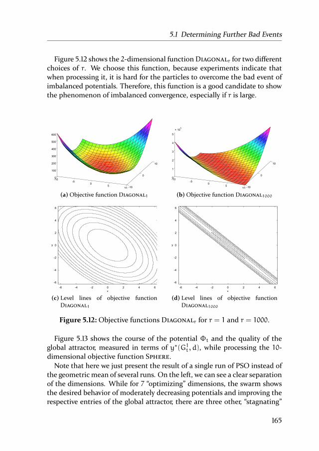
5.1 Determining Further Bad Events
Figure 5.12 shows the 2-dimensional functionDIAGONALr for two different
choices of r. We choose this function, because experiments indicate that
when processing it, it is hard for the particles to overcome the bad event of
imbalanced potentials. Therefore, this function is a good candidate to show
the phenomenon of imbalanced convergence, especially if r is large.
-10-5
05
10 -10
0
10
0
100
200
300
400
500
600
(a)Objective function DIAGONAL1
-10-5
05
10 -10
0
10
0
1
2
3
4
5
× 105
(b)Objective function DIAGONAL1000
x
y
-6 -4 -2 0 2 4 6
-6
-4
-2
0
2
4
6
(c) Level lines of objective function
DIAGONAL1
x
y
-6 -4 -2 0 2 4 6
-6
-4
-2
0
2
4
6
(d) Level lines of objective function
DIAGONAL1000
Figure 5.12:Objective functions DIAGONALr for r = 1 and r = 1000.
Figure 5.13 shows the course of the potential Φt and the quality of the
global attractor, measured in terms of y∗(G1t , d), while processing the 10-
dimensional objective function SPHERE.
Note that here we just present the result of a single run of PSO instead of
the geometric mean of several runs. On the left, we can see a clear separation
of the dimensions. While for 7 “optimizing” dimensions, the swarm shows
the desired behavior of moderately decreasing potentials and improving the
respective entries of the global attractor, there are three other, “stagnating”
165

5. Convergence for Multidimensional Problems
0 1 2 3 4 5 6 7 8 9 1010-1500
10-1000
10-500
100
× 105
6 6.05 6.1 6.15 6.2 6.25 6.3 6.35 6.4 6.45 6.510-380
10-370
10-360
10-350
10-340
10-330
10-320
10-310
× 105
dimension 1
dimension 3
dimension 5
dimension 6
dimension 7
dimension 8
dimension 9
optimizing dimensions
stagnating dimensions
(a) Potential curve of N = 3 particles processing the 10-dimensional function SPHERE.
0 1 2 3 4 5 6 7 8 9 1010-1200
10-1000
10-800
10-600
10-400
10-200
100
10200
× 105
6 6.05 6.1 6.15 6.2 6.25 6.3 6.35 6.4 6.45 6.510-730
10-720
10-710
10-700
10-690
10-680
10-670
10-660
10-650
10-640
10-630
× 105
dimension 1
dimension 3
dimension 5
dimension 6
dimension 7
dimension 8
dimension 9
stagnating dimensions
optimizing dimensions
(b) Curve of the global attractor getting improved over time.
Figure 5.13: Particle swarm suffering from imbalanced potentials while pro-
cessing 10-dimensional objective function SPHERE with N = 3
particles. Dimensions 2, 4 and 10 stagnate and are not opti-
mized.
dimensions (dimension 2, dimension 4 and dimension 10 in Figure 5.13), for
which the swarm shows a completely different behavior. For this dimensions,
the potential decreases much faster than for the optimizing ones, while the
respective coordinates of the global attractor are not significantly improved.
The result is a swarm that optimizes only a 7-dimensional problem by ignor-
ing the 3 stagnating dimensions.
At the right part of Figure 5.13, an enlarged part of the process is shown, re-
stricted to the optimizing dimensions. We can see the phases, during which
the swarm becomes running into one of the 7 optimizing dimensions, typ-
ically the one with the worst entry of the global attractor since this is the
166

5.1 Determining Further Bad Events
dimension with the largest gradient. The lengths of the running phases dif-
fer widely. Sometimes the swarm is running for more than 100 iterations,
sometimes it is only running for very few iterations. Between such running
phases, there are imbalanced phases during which one or more than one di-
mension improve their corresponding entries of the global attractor while
others have a too low potential to contribute much to the decisions on at-
tractor updates.
An explanation for this separation of the dimensions is as follows. During
a running phase, the dimension d0, in which the swarm is running, gains
more potential than the others. Assuming that at some point d0 becomes
the dimension with the highest potential, the imbalance between d0 and
the dimension with the lowest potential increases. After some iterations,
the running phase stops. As described before, from that moment on, the
more influence the d’th components have on decisions about attractor up-
dates, the faster does the potential in this dimension d decrease. Therefore,
this phase tends to rebalance the potentials in the different dimensions until
one dimension d1, which until then had only little influence on the attractor
updates, regains sufficient influence, such that the swarm becomes running
in dimension d1. However, d1 is not necessarily the dimension with the low-
est potential. The influence of a dimension on attractor updates depends on
two factors, namely the potential in this dimension and the absolute value
of the objective function’s derivative in this dimension. While stagnating di-
mensions typically have the larger derivative because the corresponding en-
tries are farther away from the optimal point where the derivative is 0, they
have a much smaller potential. Therefore, if the potential of a dimension
is too small, then the probability that the swarm becomes running in this
dimension is also very small.
Over the time, the swarm becomes running in the different optimizing
dimensions but never in the stagnating dimensions, therefore the running
phases increase the imbalance of the potentials between the optimizing and
the stagnating dimensions sufficiently fast to compensate both, the decreas-
ing derivative in the optimizing dimensions and the short imbalanced phases.
As a result, there is a critical number Dopt of dimensions which are op-
timized, i. e., if Dopt dimensions alternate in becoming running, then the
imbalance between those Dopt dimensions and the remaining dimensions
grows fast enough to maintain the separation.
This number Dopt depends on the objective function and on the swarm
size, because the number of particles determines the shape of the running
phases. Experiments indicate that a larger swarm size results in a largerDopt.
167

5. Convergence for Multidimensional Problems
That is because the effect that allows the swarm to partially balance the po-
tentials of the different dimensions is strengthened by a larger swarm size.
See also Figure 5.9, containing the results of Experiment 5.3, where we can
see that in the 2-dimensional case, a larger swarm heals itself faster from
imbalanced potentials.
0 1 2 3 4 5 6 7 8 9 1010-3500
10-3000
10-2500
10-2000
10-1500
10-1000
10-500
100
× 105
6 6.05 6.1 6.15 6.2 6.25 6.3 6.35 6.4 6.45 6.510-240
10-235
10-230
10-225
10-220
10-215
10-210
10-205
10-200
10-195
10-190
× 105
dimension 1
dimension 2
dimension 6optimizing dimensions
stagnating dimensions
(a) Potential curve of N = 2 particles processing the 10-dimensional function DIAGONAL1.
0 1 2 3 4 5 6 7 8 9 1010-700
10-600
10-500
10-400
10-300
10-200
10-100
100
10100
× 105
6 6.05 6.1 6.15 6.2 6.25 6.3 6.35 6.4 6.45 6.510-450
10-440
10-430
10-420
10-410
10-400
10-390
10-380
× 105
dimension 1
dimension 2
dimension 6
stagnating dimensions
optimizing dimensions
(b) Curve of the global attractor getting improved over time.
Figure 5.14: Particle swarm suffering from imbalanced potentials while
processing 10-dimensional objective function DIAGONAL1 with
N = 2 particles. Only dimensions 1, 2 and 6 are optimized.
Analyzing the influence of the objective function is not that simple. A
function that turns out to be difficult to optimize and yields only a smallDopt
is the functionDIAGONALr (see Figure 5.12), particularly for large values of r.
In Figure 5.14, we can see that in case of objective function DIAGONAL1 and
withN = 2 particles, the number of optimizing dimensions isDopt = 3. If ris increased and the swarm processes the functionDIAGONAL1000, then there
168

5.1 Determining Further Bad Events
0 1 2 3 4 5 6 7 8 9 1010-4500
10-4000
10-3500
10-3000
10-2500
10-2000
10-1500
10-1000
10-500
100
× 105
6 6.05 6.1 6.15 6.2 6.25 6.3 6.35 6.4 6.45 6.510-375
10-370
10-365
10-360
10-355
10-350
10-345
× 105
dimension 2
dimension 4optimizing dimensions
stagnating dimensions
(a) Potential curve ofN = 3 particles processing the 10-dimensional functionDIAGONAL1000.
0 1 2 3 4 5 6 7 8 9 1010-1200
10-1000
10-800
10-600
10-400
10-200
100
10200
× 105
6 6.05 6.1 6.15 6.2 6.25 6.3 6.35 6.4 6.45 6.510-750
10-740
10-730
10-720
10-710
10-700
10-690
× 105
dimension 2
dimension 4stagnating dimensions
optimizing dimensions
(b) Curve of the global attractor getting improved over time.
Figure 5.15: Particle swarm suffering from imbalanced potentials while pro-
cessing 10-dimensional objective function DIAGONAL1000 with
N = 3 particles. Only dimensions 2 and 4 are optimized.
are onlyDopt = 2 optimizing dimensions, which is due to the considerations
from the 2-dimensional case theminimumvalue ofDopt for any combination
of a swarm size N ≥ 2 and an objective function f(~x) = ~xt · A · ~x with a
positive-definite matrix A.
Provided with one additional particle, the swarm is able to optimize the
function DIAGONAL1000 in 3 dimensions. The results of an example run are
presented in Figure 5.16.
If we restrict theD-dimensional function SPHERE to a (D−k)-dimensional
function by fixing k components of the input vector, the result is a (possibly
shifted) version of the (D− k)-dimensional objective function SPHERE. The
same holds for the function DIAGONALr. Therefore, the number Dopt is for
169

5. Convergence for Multidimensional Problems
0 1 2 3 4 5 6 7 8 9 1010-800
10-700
10-600
10-500
10-400
10-300
10-200
10-100
100
10100
× 105
6 6.05 6.1 6.15 6.2 6.25 6.3 6.35 6.4 6.45 6.510-160
10-155
10-150
10-145
10-140
10-135
10-130
× 105
dimension 2
dimension 3
dimension 6
stagnating dimensions
optimizing dimensions
(a) Potential curve ofN = 4 particles processing the 10-dimensional functionDIAGONAL1000.
0 1 2 3 4 5 6 7 8 9 1010-500
10-400
10-300
10-200
10-100
100
10100
× 105
6 6.05 6.1 6.15 6.2 6.25 6.3 6.35 6.4 6.45 6.510-300
10-295
10-290
10-285
10-280
10-275
10-270
10-265
× 105
dimension 2
dimension 3
dimension 6stagnating dimensions
optimizing dimensions
(b) Curve of the global attractor getting improved over time.
Figure 5.16: Particle swarm suffering from imbalanced potentials while pro-
cessing 10-dimensional objective function DIAGONAL1000 with
N = 4 particles. Only dimensions 2, 3 and 6 are optimized.
both functions independent of the search space dimension D, unless D is
too small for any stagnating dimensions to occur. E. g., withN = 3 particles,we haveDopt = minD, 7 for the objective function SPHEREwith an arbitrary
dimension D. The same holds for the function DIAGONALr.
For objective functions that are less symmetric, the situation is different
and no fixed value Dopt can be given. As an example, Figure 5.17 and Figure
5.18 each show the results of a run, in which a swarm of N = 3 particles
processes the 20-dimensional objective function SCHWEFEL. However, as we
can see, in the first case, there are Dopt = 4 optimizing dimensions, while
in the second case, it turns out that Dopt = 5 dimensions are optimizing.
The reason for this is that objective function SCHWEFEL is not symmetric
170

5.1 Determining Further Bad Events
0 1 2 3 4 5 6 7 8 9 1010-3000
10-2500
10-2000
10-1500
10-1000
10-500
100
10500
× 105
6 6.005 6.01 6.015 6.02 6.025 6.03 6.035 6.04 6.045 6.0510-668
10-666
10-664
10-662
10-660
10-658
10-656
× 105
dimension 1
dimension 3
dimension 4
dimension 9optimizing dimensions
stagnating dimensions
(a) Potential curve of N = 3 particles processing the 20-dimensional function SCHWEFEL.
0 1 2 3 4 5 6 7 8 9 1010-2500
10-2000
10-1500
10-1000
10-500
100
10500
× 105
6 6.005 6.01 6.015 6.02 6.025 6.03 6.035 6.04 6.045 6.0510-1330
10-1328
10-1326
10-1324
10-1322
10-1320
10-1318
10-1316
10-1314
10-1312
× 105
dimension 1
dimension 3
dimension 4
dimension 9
stagnating dimensions
optimizing dimensions
(b) Curve of the global attractor getting improved over time.
Figure 5.17: Particle swarm suffering from imbalanced potentials while pro-
cessing 20-dimensional objective function SCHWEFEL withN =3 particles. Only dimensions 1, 3, 4 and 9 are optimized.
and in contrast to objective functions SPHERE and DIAGONALr not invariant
under permutations of the dimensions. Therefore, some dimensions of the
function SCHWEFEL are harder to optimize than others.
It is unclear if there is a swarm sizeNopt, such that a swarm of size at least
Nopt can optimize any objective function f(~x) = ~xt · A · ~x with a positive-
definite matrix A and any search space dimension D. It is even unclear if
for a fixed search space dimension D, there is a value Nopt(D) such that a
swarm of at least Nopt(D) particles can optimize any function of the given
form. E. g., forD = 10 andNopt(D) = 5, no stagnating dimensions occurred
while processing any of the considered objective functions.
171

5. Convergence for Multidimensional Problems
0 1 2 3 4 5 6 7 8 9 1010-2000
10-1500
10-1000
10-500
100
10500
× 105
6 6.005 6.01 6.015 6.02 6.025 6.03 6.035 6.04 6.045 6.0510-310
10-308
10-306
10-304
10-302
10-300
10-298
10-296
10-294
10-292
× 105
dimension 2
dimension 12
dimension 14
dimension 15
dimension 17
optimizing dimensions
stagnating dimensions
(a) Potential curve of N = 3 particles processing the 20-dimensional function SCHWEFEL.
0 1 2 3 4 5 6 7 8 9 1010-1200
10-1000
10-800
10-600
10-400
10-200
100
10200
× 105
6 6.005 6.01 6.015 6.02 6.025 6.03 6.035 6.04 6.045 6.0510-608
10-606
10-604
10-602
10-600
10-598
10-596
10-594
10-592
10-590
10-588
× 105
dimension 2
dimension 12
dimension 14
dimension 15
dimension 17
stagnating dimensions
optimizing dimensions
(b) Curve of the global attractor getting improved over time.
Figure 5.18: Particle swarm suffering from imbalanced potentials while pro-
cessing 20-dimensional objective function SCHWEFELwithN =3 particles. Only dimensions 2, 12, 14, 15 and 17 are optimized.
The optimization speed heavily depends on the swarm size and using a
swarm size of more thanNopt(D) particles might pay off. As an example for
the dependency of the optimization speed on the objective function and the
swarm size, see Figure 5.19. In Figure 5.19a and 5.19a, we can see the com-
paratively high optimization speed when optimizing the objective function
SPHERE with a swarm size of N = 3 particles. In Figure 5.19c and 5.19d, we
use the same swarm size to optimizeDIAGONAL1000. One can clearly see that
the optimization speed is orders of magnitudes slower than when SPHERE is
processed, i. e., after the same time in which the swarm processing SPHERE
approaches the optimum up to a distance of < 10−7500 in every dimension,
the swarm optimizing DIAGONAL1000 still has a distance > 10−35
to the opti-
172
5.1 Determining Further Bad Events
mum. Here, increasing the swarm size pays off. Figures 5.19e and 5.19f show
a swarm with 10 particles processing again DIAGONAL1000. After 500.000 it-
erations, the same number of function evaluations are used as in case of a
swarm with sizeN = 5 after 1.000.000 iterations, but the obtained value has
already a distance of ≈ 10−400 to the optimum.
Finding the exact values Nopt(D), the minimal swarm size for allowing
the swarm to optimize at all, and the optimal swarm size that results in the
fastest optimization, remain interesting and promising topics for future re-
search.
173

5. Convergence for Multidimensional Problems
0 1 2 3 4 5 6 7 8 9 1010-3500
10-3000
10-2500
10-2000
10-1500
10-1000
10-500
100
× 105
(a) Potential curve ofN = 5 particlesprocessing 10-dimensional func-
tion SPHERE.
0 1 2 3 4 5 6 7 8 9 1010-7000
10-6000
10-5000
10-4000
10-3000
10-2000
10-1000
100
× 105
(b) Curve of the global attractor get-
ting improved over time.
0 1 2 3 4 5 6 7 8 9 1010-40
10-35
10-30
10-25
10-20
10-15
10-10
10-5
100
105
× 105
(c) Potential curve ofN = 5 particlesprocessing 10-dimensional func-
tion DIAGONAL1000.
0 1 2 3 4 5 6 7 8 9 1010-35
10-30
10-25
10-20
10-15
10-10
10-5
100
× 105
(d) Curve of the global attractor get-
ting improved over time.
0 1 2 3 4 5 6 7 8 9 1010-450
10-400
10-350
10-300
10-250
10-200
10-150
10-100
10-50
100
1050
× 105
(e) Potential curve of N = 10 par-
ticles processing 10-dimensional
function DIAGONAL1000.
0 1 2 3 4 5 6 7 8 9 1010-900
10-800
10-700
10-600
10-500
10-400
10-300
10-200
10-100
100
× 105
(f ) Curve of the global attractor get-
ting improved over time.
Figure 5.19: Influence of objective function and swarm size on the speed
with which the particle swarm recovers from imbalanced po-
tentials.
174

5.2 ModifiedParticle SwarmOptimizationAlmost Surely Finds LocalOptima
5.2 Modified Particle Swarm Optimization Almost Surely Finds LocalOptima
Since the bad event of imbalanced potentials is a fatal event fromwhich clas-
sical PSO cannot recover on its own, we want to modify the algorithm, such
that it can overcome this particular situation, but stays as close as possible to
the classical PSO. Several modifications are possible, but in order to keep the
algorithm as simple and close to the original PSO, we propose the following
modification.
Definition 5.1 (Modified PSO). For some arbitrary small but fixed δ > 0,
we define the modified PSO via the same equations as the classic PSO in
Definition 3.8, only modifying the third part of the movement equations to
Vn,dt+1 =
(2 · rn,dt − 1) · δ,if ∀n ′ ∈ 1, ...,N : |Vn
′,dt |+ |Gn
′,dt+1 − Xn
′,dt | < δ,
χ · Vn,dt + c1 · rn,dt · (Ln,dt − Xn,dt )
+ c2 · sn,dt · (Gn,dt+1 − Xn,dt ),
otherwise.
Whenever the first case applies, we call the step and the whole iteration
forced.
An algorithmic overview over the modified PSO is given in Algorithm 4.
In words: As soon as in one dimension the sum of the velocity and the dis-
tance between the position and the global attractor are below the bound of
δ for every single particle, the updated velocity of this dimension is drawn
u. a. r. from the interval [−δ, δ]. Note the similarity between this condition
and the definition of the potential. Indeed, we could have used the condi-
tion Φn,dt+1 < δ (with some fixed a) or∑Nn=1 Y
n,dt < δ instead, but the mod-
ification as defined in Definition 5.1 is chosen to be as simple, natural and
independent from the terms occurring in the analysis as possible. Now the
phenomenon of imbalanced convergence can no longer occur because if the
potential decreases below a certain bound, a random value, which on expec-
tation has an absolute value of δ/2, is assigned to the velocity. Therefore, the
potential of every dimension has a stochastic lower bound.
This modified PSO is similar to the Noisy PSO proposed by Lehre and
Witt in [LW11] where the authors generally add a randomperturbation drawn
175

5. Convergence for Multidimensional Problems
Algorithm 4: modified PSO
input : Objective function f : S→ R to be minimized
output: G ∈ RD
// Initialization1 for n = 1→ N do2 Initialize position Xn ∈ RD randomly;
3 Initialize velocity Vn ∈ RD;4 Initialize local attractor Ln := Xn;
5 Initialize G := argminL1,...,Ln f;
// Movement6 repeat7 for n = 1→ N do8 for d = 1→ D do9 if ∀n ′ ∈ 1, ...,N : |Vn
′,d|+ |Gd − Xn′,d| < δ then
10 Vn,d := (2 · rand() − 1) · δ;11 else12 Vn,d := χ · Vn,d + c1 · rand() · (Ln,d − Xn,d)
+ c2 · rand() · (Gd − Xn,d);13 Xn,d := Xn,d + Vn,d;
14 if f(Xn) ≤ f(Ln) then Ln := Xn;15 if f(Xn) ≤ f(G) then G := Xn;
16 until termination criterion met;
u. a. r. from [−δ/2, δ/2] for some small δ and prove that their swarm is able
to find a local optimum. However, their analysis is restricted to one specific
1-dimensional objective function.
Another famous modified version of PSO with a comparable modifica-
tion is the Guaranteed Convergence PSO (GCPSO) found in [vdBE02] (see
Chapter 2, Section 2.3.3). Here, the authors made more complex changes
of the movement equations, enabling the particles to count the number of
times they improved the global attractor and use that information. Empirical
evidence for the capability of the GCPSO to find local optima on common
benchmarks is given.
In case of the proposed modified PSO, the change from the classic PSO
are considered comparatively simple. The main difference to previous ap-
proaches (e. g., [vdBE02]) is that our PSO uses the modification not as its
176

5.2 ModifiedParticle SwarmOptimizationAlmost Surely Finds LocalOptima
engine. Rather, it will turn out that the number of forced steps is small and
if the swarm is not already within an δ-neighborhood of a local optimum,
after some forced steps the potential increases and the swarm switches back
to classical steps, a behavior which can also be observed experimentally (see
Section 5.3.4)
Note that, however, the convergence of the swarm is sacrificed in order to
increase the quality of the solution, since the potential cannot approach 0
anymore. Instead, we can only expect the global attractor to converge. Pre-
sumably, we can hope for linear convergence speed until the distance to the
optimum is of order δ. From that moment on, the global attractor will still
continue converging towards the optimum, but the speed decreases signifi-
cantly because the swarm is only driven by its modification, which leads to a
behavior similar to “blind search” over some interval of size δ. However, since
δ is a user-defined parameter which can be made arbitrarily small, any prac-
tical application can take this behavior into account and choose the value δ
according to the desired precision of the result.
Now the question arises how much of the results from the 1-dimensional
PSO can be transferred to the general, D-dimensional case. Although a rig-
orous runtime analysis is generally hardly possible because the influence of
the objective function and its derivatives is not easy to handle, we can indeed
prove that the modified PSO algorithm finds local optima similar to the un-
modified PSO in the 1-dimensional case for a comparatively large class of
objective functions. For technical reasons, additionally to the requirements
of Definition 4.1, in this section we assume that the objective function f has
a continuous first derivative. This leads to the following definition of admis-
sible objective functions.
Definition 5.2. Let f : RD → R be a function. f ∈ F if and only if
(i) there is a compact set K ⊂ RD with positive Lebesgue measure, such
that P(Xn0 ∈ K) = 1 for every n and
x ∈ RD
∣∣ f(x) ≤ supK f(the
island) is bounded;
(ii) f ∈ C1(RD), i. e., f is continuous and has a continuous derivative.
For objective functions satisfying the requirements of Definition 5.2, we
prove the following theorem, which is the D-dimensional counterpart to
Theorem 4.1.
Theorem 5.1. Using the modified PSO algorithm, every accumulation point
of G = (Gnt )n=1,...,N;t∈N is a local minimum of f almost surely.
177

5. Convergence for Multidimensional Problems
Proof. Assume, for contradiction, that there is some accumulation point z of
G that is no local minimum. Then, in any neighborhood of z and therefore
in particular in Bδ(z), there is a point x0 ∈ Bδ(z) with f(x0) < f(z). Since fis continuous, x0 has some neighborhood Bτ(x0), such that f(x) < f(z) forevery x ∈ Bτ(x0). Figure 5.20 gives an overview over the situation.
Figure 5.20: Every point x0 with f(x0) < f(z) has a neighborhood Bτ(x0),such that f(x) < f(z) for x ∈ Bτ(x0)
The set Bτ(x0) plays the role of the interval (z, z + τ) from the proof of
Theorem 4.1. Now we investigate what happens when G enters Bε(z). Thiswill for each ε > 0 happen infinitely often because z is an accumulation
point. The modification of the PSO algorithm enables the construction of a
sequence of steps leading a particle into Bτ(x0). In principle, the sequence
can be obtained by using the sequence from the proof of Theorem 4.1 for
every single dimension. However, that may result in a particle being at the
desired positions in two distinct dimensions at two different points in time,
so the sequence is constructed basically by a simple composition of modified
sequences from Theorem 4.1 for every single dimension in which the steps
are not forced. Themodification of the sequences ensuring that they all have
the same length is straight-forward. For forced dimensions, the probability
for hitting Bτ(x0) within the next step is obviously positive and so is the
probability for obtaining a velocity suitable for ensuring that the next step
will be forced in case the other dimensions are not at the end of their se-
quences. Note that due to the modification, splitting cases on whether there
is a second accumulation point or not is unnecessary.
178

5.2 ModifiedParticle SwarmOptimizationAlmost Surely Finds LocalOptima
This result is not surprising because in the modified PSO random per-
turbations occur when the swarm tends to converge and it is easy to see that
small randomperturbations can optimize any continuous function (but with
a very poor runtime). Note that the proof of Theorem 5.1 does neither make
use of f having a continuous derivative nor of Lemma 4.1. To supplement this
result, we will prove a statement about how often the modification actually
applies. It is obvious that for δ chosen too large, the behavior of the swarm
is dominated by its forced steps. The case of δ being small with respect to
the structure of the function is the interesting one. On the other hand, if
the distance of a particle and a local optimum is smaller than δ, presumably
many of the upcoming steps will be forced because there is no room for fur-
ther improvements. But we can show that, given the swarm is sufficiently far
away from the closest local optimum, the forced steps only balance the po-
tentials between the different dimensions and enable the swarm to become
running. In particular, consider the following situation: Let for some dimen-
sion d0 and some c 1 be ∂f∂d0
< 0 on a (c · δ)-neighborhood of the current
global attractor and let the swarm have low potential, i. e., every particle has
in every dimension potential of order δ. Instead of only being driven by the
random perturbation, we would like the swarm to become running in direc-
tion d0 (or some other direction), increasing the potential in that direction,
so the velocity updates can be done according to the classical movement
equations again.
Theorem5.2. In the situation described above, the probability for the swarm
to become running within a constant number of iterations is positive and in-
dependent of δ.
Proof. We can explicitly describe a possible sequence of iterations enabling
the swarm to become running. First, the particles decrease their distance to
the global attractor in every single dimension to atmost δ·ε/2with ε 1 and
a velocity of absolute value less than δ ·(1−ε/2), such that the local attractor
is updated for all particles except the one whose local attractor is equal to
the global attractor. If the current global attractor Gnt is no local maximum,
this can be done because every local attractor has a function value worse
than the global attractor and since f is continuous, so the function values
of f approach f(Gnt ) when x approaches Gnt . The case of Gnt being a local
maximum has probability 0. Then the next step of each particle is forced.
In the next iteration, the velocity of every particle gets smaller than δ · ε/2in each dimension except d0. In dimension d0, one particle obtains velocity
greater than δ·(1+ε)/2, such that it gets to a search point that is in dimension
179

5. Convergence for Multidimensional Problems
d0 more than δ/2 and in any other dimension at most ε · δ away from the
previous global attractor. For ε sufficiently small, this particle will update
the global attractor since f has a positive partial derivative in dimension d0.
Every other particle obtains in d0 a velocity less than −δ · (1+ ε)/2, making
sure that its new position and the new global attractor after that step differ
by more than δ. So the next step will not be forced and the potentials have
order
√δ in dimension d0 and only
√δ · ε in every other dimension. So for
ε sufficiently small with respect to the function f, the swarm will become
running and therefore the steps will actually become unforced.
The behavior of the modified PSO is the same as of the classic PSO, ex-
cept that due to the modification the particles can overcome “corners,” i. e.,
in presence of imbalanced potentials, the modification helps to balance the
potentials of the different dimensions. The “blind” algorithm that just ran-
domly checks a point around the previous best solution with range δ would
of course find a local minimum, too, but with a very poor running time be-
cause it can not accelerate and therefore its step size will only be of order
δ.
5.3 Experimental Results with a Standard Implementation
To supplement the results about the behavior of PSO in that “artificial” set-
ting, we run it on twowell-known benchmark functions, using standard dou-
ble precision number and standard methods like calculation of the arith-metic mean instead of the geometric mean, to show that the bad event of
the imbalanced potentials actually occurs on common benchmark instances
and affects the optimization even under common experimental conditions.
The following experiments are performed using MATLAB version 8.2.0.701
(R2013b).
5.3.1 The Problem of Imbalanced Potentials on Standard Benchmarks
Since the described scenario may happen with positive but, depending on
the situation, small probability, we choose the number of particles N small
180

5.3 Experimental Results with a Standard Implementation
compared to the number of dimensions D in order to be able to view the
phenomenon in a preferably pure condition.
We run PSO on the objective functions SPHEREwith optimal solution z∗ =(0, ..., 0) and ROSENBROCK with optimal solution z∗ = (1, ..., 1) (found in
[Ros60]). The function ROSENBROCK is defined as follows:
ROSENBROCK(~x) =D−1∑d=1
((1− xd)
2 + 100 · (xd+1 − x2d)2).
Figure 5.21 shows the function ROSENBROCK for D = 2 dimensions.
xy
-2
-1
0
1
2
-0.500.511.522.530
500
1000
1500
2000
2500
Figure 5.21:Objective function ROSENBROCK.
Experiment 5.5. We initialize the particles’ positions uniformly at random
over [−100, 100]D and the velocities over [−50, 50]D for processing function
SPHERE. For the function ROSENBROCK, we distribute the initial popula-
tion randomly over [−5, 10]D and the initial velocity over [−2.5, 5]D. For thesearch space dimensionD = 5, we set the swarm size toN = 2 and the total
number of iterations tmax to 10.000 and for D = 50, we use N = 8 particles
and tmax = 100.000 iterations. We repeat each experiment 1000 times and
calculate the arithmetic means.
181

5. Convergence for Multidimensional Problems
Table 5.1 lists the results. For each repetition, we determine the dimen-
sion with the minimal and the one with the maximal value for the potential
Φ after the last iteration (see columns Φ), together with the difference be-
tween the global attractor and the optimal solution in the dimension with
the lowest and highest remaining potential, respectively.
Table 5.1: Imbalanced Potentials
Function Sphere Rosenbrock
D 5 50 5 50
N 2 8 2 8
tmax 10000 100000 10000 100000
Value 247.83 26.2706 4.19 · 106 4.1256 · 105
min. ΦΦ 0* 0* 0* 1.0320 · 10−5
dist. opt. - 0.9188 - 0.3235
max. ΦΦ 0* 2.2778 · 10−4 0* 0.1789
dist. opt. - 2.5449 · 10−8 - 104.2775*Due to double precision.
In the 5-dimensional case, the potential reaches 0 due to double preci-
sion in every dimension, so there is no single dimension with highest or
lowest potential. However, the function value obtained at the point where
the particles converge to is still far away from the optimum. In case of the
50-dimensional SPHERE, we can see that the dimension with the highest
value for Φ usually is much closer to its optimal value than the dimension
with the lower value. This confirms the concerns about the classical PSO
in connection with imbalanced potentials. Since function ROSENBROCK is
non-separable, the same relationship between the remaining potentials and
the distance to the optimum cannot be obtained. However, what we can see
is that the remaining potentials are much smaller than the distance to the
optimum.
5.3.2 Avoiding Imbalanced Convergence
We repeat Experiment 5.5 in the same setting as before, but using the modi-
fied PSO as defined in Definition 5.1 with δ := 10−12. The results can be seen
in Table 5.2. It turns out that the modified PSO algorithm actually leads
182
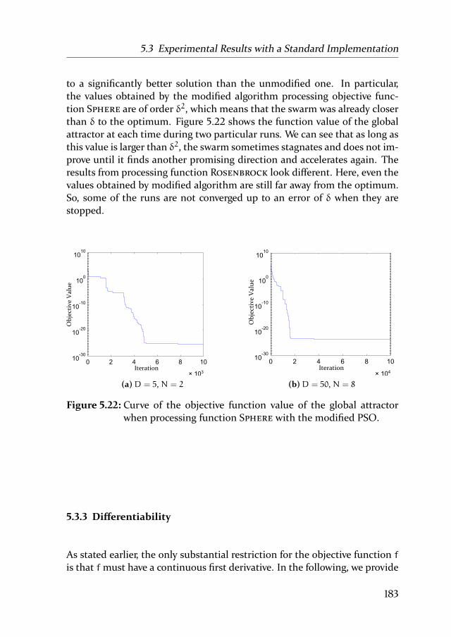
5.3 Experimental Results with a Standard Implementation
to a significantly better solution than the unmodified one. In particular,
the values obtained by the modified algorithm processing objective func-
tion SPHERE are of order δ2, which means that the swarm was already closer
than δ to the optimum. Figure 5.22 shows the function value of the global
attractor at each time during two particular runs. We can see that as long as
this value is larger than δ2, the swarm sometimes stagnates and does not im-
prove until it finds another promising direction and accelerates again. The
results from processing function ROSENBROCK look different. Here, even the
values obtained by modified algorithm are still far away from the optimum.
So, some of the runs are not converged up to an error of δ when they are
stopped.
10-30
10-20
10-10
100
1010
0 2 4 6 8 10
× 103
Ob
ject
ive
Val
ue
Iteration
(a)D = 5, N = 2
0 2 4 6 8 1010
-30
10-20
10-10
100
1010
× 104Iteration
Ob
ject
ive
Val
ue
(b)D = 50, N = 8
Figure 5.22: Curve of the objective function value of the global attractor
when processing function SPHERE with the modified PSO.
5.3.3 Differentiability
As stated earlier, the only substantial restriction for the objective function f
is that fmust have a continuous first derivative. In the following, we provide
183

5. Convergence for Multidimensional Problems
Table 5.2: Comparison between the classic and the modified PSO algorithm
Function D N tmax δ Value
Sphere 5 2 10000 10−12 1.91 · 10−26Sphere 5 2 10000 - 247.83
Sphere 50 8 100000 10−12 2.1402 · 10−24Sphere 50 8 100000 - 26.27
Rosenbrock 5 2 10000 10−12 2.67 · 105Rosenbrock 5 2 10000 - 4.19 · 106Rosenbrock 50 8 100000 10−12 220.66
Rosenbrock 50 8 100000 - 4.13 · 105
an example, showing what can happen when f is only continuous. For some
fixed b > 1, we define the D-dimensional function f as follows:
f(~x) =
∑ni=1 x
2i , ∃i, j : xi ≥ b · xj ∨ xj ≥ b · xi∑n
i=1 x2i
b− 1·(2maxi 6=j
xixj
− b− 1
), otherwise
(a) Continuous, not differentiablefunction f
(b) Particles making almost only
forced steps through the valley
Figure 5.23: (a) Function f, (b) behavior of the particles on f
Figure 5.23a shows a plot of the 2-dimensional function f. For y not be-
tween x/b and x · b, this function behaves like the well-known function
184

5.3 Experimental Results with a Standard Implementation
SPHERE. For x = y, f(x, y) = −2 · x2 and from y = x/b (y = x · b) toy = x, the function falls into a valley. It is easy to see that this function is
continuous but has no derivative. The construction of a continuous function
which behaves like f on a bounded set and tends to infinity for |x|+ |y|→∞is straightforward. Therefore, the particles must be able to pass through the
valley.
Experiment 5.6. We initialize the particles’ positions uniformly at random
over [−100; 100]D (except for the first particle, which is initialized at (1, ..., 1)such that the swarm could see the direction where the improvements are
possible) and the velocities over [−50; 50]D, with the value D = 3. We per-
form a total of 1000 runs, each with 5000 iterations. We determine the po-
tential of the dimension with the highest potential after the last iteration
and calculate the mean and standard deviation of the respective dimensions
over the 1000 repetitions. This is done for two different swarm sizes, namely
N = 10 and N = 50.
We repeat the experiment with 10 particles and only 100 iterations, using
the function frot, which is obtained by first rotating the input vector and then
applying f such that the valley now leads the particles along the x1-axis. For-
mally speaking, the rotation maps the vector (√N, 0, . . . , 0) to (1, 1, . . . , 1)
and keeps every vector that is orthogonal to this two invariant.
The results of Experiments 5.6 can be seen in Figure 5.24. In all three
cases, for about the first 20 iterations, the swarm behaves like on the function
SPHERE and reduces its potential. Then, it discovers the valley and tries to
move through it. However, in the unrotated case with 10 particles (Figure
5.24a), the swarm fails to accelerate and instead, it converges towards a non-
optimal point. With much more effort, the swarm consisting of 50 particles
(Figure 5.24b) is able to accelerate, but the acceleration rate and therefore
the speed are comparatively poor. Finally, Figure 5.24c shows how the swarm
handles the rotated version much better than the original function f before.
Here, after only 100 iterations, the potential increased to a value of about
1045. The reason for this large difference between the behavior on f and on
frot is the capability of the swarm to favor one direction only if this direction
is parallel to one of the axes.
In particular, this experiment also confirms the results in [HRM+11], name-
ly that PSO is not invariant under rotations of the search space.
185

5. Convergence for Multidimensional Problems
0 1000 2000 3000 4000 500010
0
101
102
103
Potential
Iteration
(a) Function f, b = 1.1, 10 particles
0 1000 2000 3000 4000 500010
2
103
104
Iteration
Potential
(b) Function f, b = 1.1, 50 particles
0 20 40 60 80 10010
0
1010
1020
1030
1040
1050
Potential
Iteration
(c) Function frot, b = 1.1. 10 particles
Figure 5.24: Behavior of the particles on functions f and frot
5.3.4 Impact of the Modification
To make sure that the modification does not fully take over, we track the
forced points, i. e., the positions of particles before performing a forced step,
in order to see how many of them occur and where the modification is used.
Experiment 5.7. For processing the 2-dimensional function SPHERE, we ini-
tialize the particles uniformly at random over [−100, 100] and the velocities
over [−50, 50]. We set the parameter δ to 10−7. The swarm size is set toN = 2and the number of iterations to tmax = 100.000.
The points at which particle performed a forced step can be seen in Fig-
ure 5.25.
As can be seen in the figure, the particles get forced near (−2 · 10−5, 0)but their movement does not stay forced. Instead, the swarm becomes run-
186

5.3 Experimental Results with a Standard Implementation
x
y
-3 -2 -1 0 1 2 3-3
-2
-1
0
1
2
3
× 10-5
× 10-5
Footprints of forced steps
Figure 5.25: Behavior of the modified PSO on function SPHERE
ning again until the particles approached the optimum at (0, 0). This implies
that for sufficiently smooth functions, the modification does not take over,
replacing PSO by some random search routine. Instead, the modification
just helps to overcome “corners.” As soon as there is a direction parallel to an
axis with decreasing function value, the swarm becomes running again and
the unmodified movement equations apply.
187


6. Conclusion
In this thesis, we studied the process of convergence in detail. As a main tool
for the analysis, we defined the potential of a particle swarm and analyzed
its course in order to measure, how far the swarm at a certain time is already
converged. With the help of this potential, we could prove the first main
result, namely that in a 1-dimensional situation, the swarm with probabil-
ity 1 converges towards a local optimum for a comparatively wide range of
admissible objective functions.
In order to measure the runtime, so-called bad events, i. e., situations
in which the particle swarm optimization (PSO) does not make significant
progress, where studied. We could proof that in the 1-dimensional situation,
the swarm is able to recover from encountering such a bad event within rea-
sonable time. Applying drift theory led to the second main result, namely
the formal proof that the swarm obtains a precision of k digits in timeO(k).In the general D-dimensional case, it turned out that there exists a bad
event from which the swarm is unable to recover, namely the situation when
some dimensions have a potential orders of magnitude smaller than oth-
ers. Such dimensions with a too small potential loose their influence on the
behavior of the algorithm, and therefore the respective entries are not op-
timized. In order to solve this issue, a slightly modified PSO was proposed
that again guarantees convergence towards a local optimum. Experiments
where presented, indicating that indeed the modified swarm recovers from
this bad event, and also indicating that the modification does not govern the
whole algorithm.
Directions of future research
A future research goal is to formally prove the mentioned aspects of the
swarm’s behavior in situations with more than one dimension. A first at-
tempt on this is made in [Raß14], where the author provides a theoretical
189

6. Conclusion
framework for formally proving that the swarm sometimes stagnates at lo-
cations that are no local optimum.
The technique of studying the bad events can be expanded tomore general
cases, e. g., a possible next step is to provide convergence proof and runtime
bounds for the 2-dimensional case using the unmodified PSO. Another op-
portunity lies in further studying the modified PSO from Section 5.2. As
long as k < log(1/δ), one could expect the modified PSO to obtain a preci-
sion of k digits in timeO(k). Since δ is a user-defined parameter, this can be
sufficient for practical applications.
Finally, the proposed continuous drift theorem looks promising and it is
likely that it can be applied in order to analyze other continuous optimiza-
tion heuristics. Therefore, this direction of drift theory on its own is worth
further studies in order to, e. g., generalize it to other situations on the one
hand and on the other hand specialize it in order to find tighter boundswhen
the investigated stochastic process has stronger properties, e. g., the Markov
property.
190

Bibliography
[ABEF05] Julio E. Alvarez-Benitez, Richard M. Everson, and Jonathan E.
Fieldsend. A MOPSO algorithm based exclusively on pareto
dominance concepts. In Proceedings of the Conference on Evo-lutionary Multi-Criterion Optimization (EMO), volume 3410 of
Lecture Notes in Computer Science, pages 459–473. Springer,
2005. doi:10.1007/978-3-540-31880-4_32.
[AP09] Davide Anghinolfi and Massimo Paolucci. A new discrete
particle swarm optimization approach for the single-machine
total weighted tardiness scheduling problem with sequence-
dependent setup times. European Journal of Operational Re-search, 193(1):73–85, 2009.
[AT10] Anne Auger and Olivier Teytaud. Continuous lunches are free
plus the design of optimal optimization algorithms. Algorith-mica, 57(1):121–146, 2010. doi:10.1007/s00453-008-9244-5.
[Bau96] Heinz Bauer. Probability Theory, volume 23 of Studies in Math-ematics. De Gruyter, 1996.
[BBD+09] Surender Baswana, Somenath Biswas, Benjamin Doerr, Tobias
Friedrich, Piyush P. Kurur, and Frank Neumann. Computing sin-
gle source shortest paths using single-objective fitness. In Pro-ceedings of the Tenth ACM SIGEVOWorkshop on Foundations ofGenetic Algorithms, Proceedings of the ACM SIGEVOWorkshop
on Foundations of Genetic Algorithms (FOGA), pages 59–66.
ACM, 2009. doi:10.1145/1527125.1527134.
[BF05] Bogdan Bochenek and Paweł Foryś. Structural optimization
against instability using particle swarms. In Proceedings of the6th World Congress on Structural and Multidisciplinary Opti-mization, 2005. CD-ROM Proceedings.
191

Bibliography
[BK07] Daniel Bratton and James Kennedy. Defining a standard for
particle swarm optimization. In Proceedings of the IEEESwarm Intelligence Symposium (SIS), pages 120–127, 2007.
doi:10.1109/SIS.2007.368035.
[BM06] Jürgen Branke and Sanaz Mostaghim. About selecting the
personal best in multi-objective particle swarm optimiza-
tion. In Thomas Philip Runarsson, Hans-Georg Beyer, Ed-
mund K. Burke, Juan J. Merelo Guervós, L. Darrell Whitley,
and Xin Yao, editors, Proceedings of the Conference on Paral-lel Problem Solving from Nature (PPSN), volume 4193 of Lec-ture Notes in Computer Science, pages 523–532. Springer, 2006.doi:10.1007/11844297_53.
[BM14] Mohammad Reza Bonyadi and Zbigniew Michalewicz. Spso
2011: Analysis of stability; local convergence; and rotation sen-
sitivity. In Proceedings of the 2014 Conference on Genetic andEvolutionary Computation, GECCO ’14, pages 9–16. ACM, 2014.
doi:10.1145/2576768.2598263.
[BML14] Mohammad Reza Bonyadi, Zbigniew Michalewicz, and Xi-
aodong Li. An analysis of the velocity updating rule of the parti-
cle swarm optimization algorithm. Journal of Heuristics, pages1–36, 2014. doi:10.1007/s10732-014-9245-2.
[BS02] Hans-Georg Beyer andHans-Paul Schwefel. Evolution strategies
- a comprehensive introduction. Natural Computing, 1(1):3–52,2002. doi:10.1023/A:1015059928466.
[BSMD08] Sanghamitra Bandyopadhyay, Sriparna Saha, Ujjwal Maulik,
and Kalyanmoy Deb. A simulated annealing-based mul-
tiobjective optimization algorithm: Amosa. IEEE Trans-actions on Evolutionary Computation, 12(3):269–283, 2008.
doi:10.1109/TEVC.2007.900837.
[CCZ09] Zhihua Cui, Xingjuan Cai, and Jianchao Zeng. Stochas-
tic velocity threshold inspired by evolutionary programming.
In Proceedings of the World Congress on Nature and Biologi-cally Inspired Computing (NaBIC), pages 626–631. IEEE, 2009.doi:10.1109/NABIC.2009.5393434.
192

Bibliography
[CD01] Anthony Carlisle and Gerry Dozier. An off-the-shelf PSO. In
Proceedings of the Particle SwarmOptimizationWorkshop, pages1–6, 2001.
[CK02] Maurice Clerc and James Kennedy. The particle swarm – explo-
sion, stability, and convergence in a multidimensional complex
space. IEEE Transactions on Evolutionary Computation, 6:58–73, 2002. doi:10.1109/4235.985692.
[Cle03] Maurice Clerc. Tribes, a parameter free particle swarm opti-
mizer. http://clerc.maurice.free.fr/pso/, 2003.
[Cle04] Maurice Clerc. Discrete Particle SwarmOptimization, illustratedby the Traveling Salesman Problem, pages 219–239. Springer
Berlin Heidelberg, 2004.
[Cle06a] Maurice Clerc. Confinements and biases in particle swarm op-
timisation. http://clerc.maurice.free.fr/pso/, 2006.
[Cle06b] Maurice Clerc. Stagnation analysis in particle swarm
optimization or what happens when nothing happens.
http://hal.archives-ouvertes.fr/hal-00122031, 2006. Technical
report.
[Cle07] Maurice Clerc. Back to random topology.
http://clerc.maurice.free.fr/pso/, 2007.
[Coe02] Carlos A. Coello Coello. Theoretical and numerical constraint-
handling techniques used with evolutionary algorithms: a sur-
vey of the state of the art. ComputerMethods in AppliedMechan-ics and Engineering, 191:1245–1287, 2002. doi:10.1016/s0045-
7825(01)00323-1.
[CZS06] Zhihua Cui, Jianchao Zeng, and Guoji Sun. Adaptive ve-
locity threshold particle swarm optimization. In Guoyin
Wang, James F. Peters, Andrzej Skowron, and Yiyu Yao, ed-
itors, Proceedings of the International Conference on RoughSets and Knowledge Technology (RSKT), volume 4062 of Lec-ture Notes in Computer Science, pages 327–332. Springer, 2006.doi:10.1007/11795131_47.
193

Bibliography
[DG97] Marco Dorigo and Luca Maria Gambardella. Ant colony system:
A cooperative learning approach to the traveling salesman prob-
lem. IEEE Transactions on Evolutionary Computation, 1(1):53–66, 1997. doi:10.1109/4235.585892.
[DG10] Benjamin Doerr and Leslie Ann Goldberg. Drift analysis
with tail bounds. In Robert Schaefer, Carlos Cotta, Joanna
Kolodziej, and Günter Rudolph, editors, Parallel Problem Solv-ing fromNature, PPSNXI, volume 6238 of Lecture Notes in Com-puter Science, pages 174–183. Springer Berlin Heidelberg, 2010.
doi:10.1007/978-3-642-15844-5_18.
[DJ10] Benjamin Doerr and Daniel Johannsen. Edge-based represen-
tation beats vertex-based representation in shortest path prob-
lems. In Proceedings of the Conference on Genetic and Evo-lutionary Computation (GECCO), pages 759–766. ACM, 2010.
doi:10.1145/1830483.1830618.
[DJW02] Stefan Droste, Thomas Jansen, and Ingo Wegener. On the
analysis of the (1+1) evolutionary algorithm. TheoreticalComputer Science, 276(1–2):51–81, 2002. doi:10.1016/S0304-
3975(01)00182-7.
[DJW12] Benjamin Doerr, Daniel Johannsen, and Carola Winzen. Mul-
tiplicative drift analysis. Algorithmica, 64(4):673–697, 2012.doi:10.1007/s00453-012-9622-x.
[dSC08] Leandro dos Santos Coelho. A quantum particle swarm opti-
mizer with chaotic mutation operator. Chaos, Solitons & Frac-tals, 37(5):1409–1418, 2008.
[EK95] Russell C. Eberhart and James Kennedy. A new optimizer using
particle swarm theory. In Proceedings of the 6th InternationalSymposium onMicroMachine andHuman Science, pages 39–43,1995. doi:10.1109/MHS.1995.494215 .
[Fan02] Huiyuan Fan. A modification to particle swarm optimization
algorithm. Engineering Computations, 19(7-8):970–989, 2002.doi:10.1108/02644400210450378.
[FG02] P. C. Fourie and Albert A. Groenwold. The particle swarm op-
timization algorithm in size and shape optimization. Struc-
194

Bibliography
tural and Multidisciplinary Optimization, 23:259–267, 2002.
doi:10.1007/s00158-002-0188-0.
[GADP89] S. Goss, Serge Aron, Jean L. Deneubourg, and Jacques Pas-
teels. Self-organized shortcuts in the argentine ant. Naturwis-senschaften, 76(12):579–581, 1989. doi:10.1007/bf00462870.
[GAHG05] Crina Grosan, Ajith Abraham, Sangyong Han, and Alexander F.
Gelbukh. Hybrid particle swarm - evolutionary algorithm for
search and optimization. In Proceedings of the Mexican In-ternational Conference on Artificial Intelligence (MICAI), vol-ume 3789 of Lecture Notes in Computer Science, pages 623–632.Springer, 2005. doi:10.1007/11579427_63.
[GW03] Oliver Giel and Ingo Wegener. Evolutionary algorithms and the
maximummatching problem. In Helmut Alt andMichel Habib,
editors, STACS 2003, volume 2607 of Lecture Notes in Com-puter Science, pages 415–426. Springer Berlin Heidelberg, 2003.
doi:10.1007/3-540-36494-3_37.
[GWHK09] Alexandr Gnezdilov, Stefan Wittmann, Sabine Helwig, and
Gabriella Kókai. Acceleration of a relative positioning frame-
work. International Journal of Computational Intelligence Re-search, 5:130–140, 2009.
[Haj82] BruceHajek. Hitting-time and occupation-time bounds implied
by drift analysis with applications. Advances in Applied Proba-bility, 14(3):502–525, 1982.
[HBM13] Sabine Helwig, Jürgen Branke, and Sanaz Mostaghim. Experi-
mental analysis of bound handling techniques in particle swarm
optimization. IEEE Transactions on Evolutionary Computation,17(2):259–271, April 2013. doi:10.1109/TEVC.2012.2189404 .
[HE02a] Xiaohui Hu and Russell Eberhart. Multiobjective optimiza-
tion using dynamic neighborhood particle swarm optimization.
In Proceedings of the IEEE Congress on Evolutionary Computa-tion (CEC), pages 1677–1681, Washington, DC, USA, 2002. IEEE
Computer Society. doi:10.1109/CEC.2002.1004494 .
[HE02b] Xiaohui Hu and Russell Eberhart. Solving constrained nonlin-
ear optimization problems with particle swarm optimization.
195

Bibliography
In Proceedings of the 6th World Multiconference on Systemics,Cybernetics and Informatics (SCI), pages 203–206, 2002.
[Hel10] Sabine Helwig. Particle Swarms for Constrained Optimization.PhD thesis, Department of Computer Science, University of
Erlangen-Nuremberg, 2010. urn:nbn:de:bvb:29-opus-19334.
[HES03a] Xiaohui Hu, Russell C. Eberhart, and Yuhui Shi. Engineer-
ing optimization with particle swarm. In Proceedings of theIEEE Swarm Intelligence Symposium (SIS), pages 53–57, 2003.
doi:10.1109/SIS.2003.1202247.
[HES03b] Xiaohui Hu, Russell C. Eberhart, and Yuhui Shi. Swarm intelli-
gence for permutation optimization: a case study of n-queens
problem. In Proceedings of the IEEE Swarm Intelligence Sympo-sium (SIS), pages 243–246, 2003. doi:10.1109/SIS.2003.1202275.
[HM06] Werner Halter and Sanaz Mostaghim. Bilevel optimiza-
tion of multi-component chemical systems using particle
swarm optimization. In Proceedings of the IEEE Congresson Evolutionary Computation (CEC), pages 1240–1247, 2006.
doi:10.1109/CEC.2006.1688451.
[HNW09] Sabine Helwig, Frank Neumann, and Rolf Wanka. Particle
swarm optimization with velocity adaptation. In Proceedingsof the International Conference on Adaptive and Intelligent Sys-tems (ICAIS), pages 146–151, 2009. doi:10.1109/ICAIS.2009.32.
[HRM+11] Nikolaus Hansen, Raymond Ros, Nikolas Mauny, Marc Schoe-
nauer, and Anne Auger. Impacts of invariance in search:
When CMA-ES and PSO face ill-conditioned and non-separable
problems. Applied Soft Computing, 11:5755–5769, 2011.
doi:10.1016/j.asoc.2011.03.001 .
[HW08] Sabine Helwig and Rolf Wanka. Theoretical analysis of ini-
tial particle swarm behavior. In Proceedings of the 10th In-ternational Conference on Parallel Problem Solving from Nature(PPSN), pages 889–898, 2008. doi:10.1007/978-3-540-87700-
4_88.
196
Bibliography
[HY01] Jun He and Xin Yao. Drift analysis and average time complexity
of evolutionary algorithms. Artificial Intelligence, 127(1):57–85,2001. doi:10.1016/S0004-3702(01)00058-3.
[HY04] Jun He and Xin Yao. A study of drift analysis for estimating com-
putation time of evolutionary algorithms. Natural Computing,3(1):21–35, 2004. doi:10.1023/B:NACO.0000023417.31393.c7.
[ Jäg03] Jens Jägersküpper. Analysis of a simple evolutionary algorithm
for minimization in euclidean spaces. In Jos C. M. Baeten,
Jan Karel Lenstra, JoachimParrow, andGerhard J.Woeginger, ed-
itors, Proceedings of the International Colloquium on Automata,Languages, and Programming (ICALP), volume 2719 of LectureNotes in Computer Science, pages 1068–1079. Springer, 2003.
doi:10.1007/3-540-45061-0_82.
[Jäg07] Jens Jägersküpper. Algorithmic analysis of a basic evolutionary
algorithm for continuous optimization. Theoretical ComputerScience, 379(3):329–347, 2007. doi:0.1016/j.tcs.2007.02.042.
[Jäg08] Jens Jägersküpper. A blend of markov-chain and drift analysis.
In Günter Rudolph, Thomas Jansen, Simon Lucas, Carlo Poloni,
andNicola Beume, editors, Parallel Problem Solving fromNature– PPSN X, volume 5199 of Lecture Notes in Computer Science,pages 41–51. Springer BerlinHeidelberg, 2008. doi:10.1007/978-
3-540-87700-4_5.
[JHW08] Johannes Jordan, Sabine Helwig, and Rolf Wanka. Social in-
teraction in particle swarm optimization, the ranked FIPS, and
adaptive multi-swarms. In Proceedings of the Genetic and Evolu-tionary Computation Conference (GECCO), pages 49–56, 2008.doi:10.1145/1389095.1389103.
[JLY07a] Ming Jiang, Yupin P. Luo, and Shiyuan Y. Yang. Particle swarm
optimization – stochastic trajectory analysis and parameter se-
lection. In Felix T. S. Chan and Manoj Kumar Tiwari, editors,
Swarm Intelligence – Focus on Ant and Particle SwarmOptimiza-tion, pages 179–198. I-TECH Education and Publishing, 2007.
Corrected version of [JLY07b].
[ JLY07b] Ming Jiang, Yupin P. Luo, and Shiyuan Y. Yang. Stochas-
tic convergence analysis and parameter selection of the stan-
197

Bibliography
dard particle swarm optimization algorithm. Information Pro-cessing Letters (IPL), 102:8–16, 2007. Corrected by [JLY07a],
doi:10.1016/j.ipl.2006.10.005.
[JM05] Stefan Janson and Martin Middendorf. A hierarchical particle
swarm optimizer and its adaptive variant. IEEE Transactions onSystems, Man, and Cybernetics, Part B, 35(6):1272–1282, 2005.doi:10.1109/TSMCB.2005.850530.
[KE95] James Kennedy and Russell C. Eberhart. Particle swarm op-
timization. In Proceedings of the IEEE International Confer-ence on Neural Networks, volume 4, pages 1942–1948, 1995.
doi:10.1109/ICNN.1995.488968 .
[KE97] James Kennedy and Russell C. Eberhart. A discrete binary ver-
sion of the particle swarm algorithm. In Proceedings of theIEEE International Conference on Systems, Man, and Cybernet-ics, volume 5, pages 4104–4108. IEEE Computer Society, 1997.
doi:10.1109/ICSMC.1997.637339 .
[Ken97] James Kennedy. The particle swarm: Social adaptation of
knowledge. In Proceedings of the IEEE International Confer-ence on Evolutionary Computation (ICEC), pages 303–308, 1997.doi:10.1109/ICEC.1997.592326.
[Ken99] James Kennedy. Small worlds andmega-minds: effects of neigh-
borhood topology on particle swarm performance. In Proceed-ings of the Congress on Evolutionary Computation (CEC), vol-ume 3, pages 1931–1938, 1999. doi:10.1109/CEC.1999.785509.
[Ken03] James Kennedy. Bare bones particle swarms. In Proceedingsof the IEEE Swarm Intelligence Symposium (SIS), pages 80–87,
2003. doi:10.1109/SIS.2003.1202251.
[KGV83] Scott Kirkpatrick, C. D. Gelatt, and M. P. Vecchi. Optimiza-
tion by simulated annealing. Science, 220(4598):671–680, 1983.doi:10.1126/science.220.4598.671.
[Kle06] Achim Klenke. Wahrscheinlichkeitstheorie. Springer Berlin Hei-
delberg New York, 2006.
198
Bibliography
[KM02] James Kennedy and Rui Mendes. Population structure and par-
ticle swarm performance. In Proceedings of the Congress on Evo-lutionary Computation (CEC), volume 2, pages 1671–1676, 2002.
doi:10.1109/CEC.2002.1004493.
[KM06] James Kennedy and Rui Mendes. Neighborhood topolo-
gies in fully informed and best-of-neighborhood particle
swarms. Systems, Man, and Cybernetics, Part C: Applica-tions and Reviews, IEEE Transactions on, 36(4):515–519, 2006.doi:10.1109/TSMCC.2006.875410.
[KSF06] Visakan Kadirkamanathan, Kirusnapillai Selvarajah, and Peter J.
Fleming. Stability analysis of the particle dynamics in particle
swarm optimizer. IEEE Transactions on Evolutionary Computa-tion, 10(3):245–255, 2006. doi:10.1109/TEVC.2005.857077.
[LS05a] J. J. Liang and Ponnuthurai N. Suganthan. Dynamic multi-
swarm particle swarm optimizer. In Proceedings of the IEEESwarm Intelligence Symposium (SIS), pages 124–129, 2005.
doi:10.1109/SIS.2005.1501611.
[LS05b] J. J. Liang and Ponnuthurai N. Suganthan. Dynamic multi-
swarm particle swarm optimizer with local search. In Proceed-ings of the Congress on Evolutionary Computation (CEC), vol-ume 1, pages 522–528, 2005. doi:10.1109/CEC.2005.1554727.
[LT01] Panta Lucic and Dusan Teodorovic. Bee system: modeling com-
binatorial optimization transportation engineering problems
by swarm intelligence. Preprints of the TRISTAN IV triennialsymposium on transportation analysis, pages 441–445, 2001.
[LW11] Per Kristian Lehre and Carsten Witt. Finite first hitting time
versus stochastic convergence in particle swarm optimisation,
2011. arXiv:1105.5540.
[MC99] Jacqueline Moore and Richard Chapman. Application of par-
ticle swarm to multiobjective optimization. Department of
Computer Science and Software Engineering, Auburn Univer-
sity. (Unpublished manuscript), 1999.
[MF02] Vladimiro Miranda and Nuno Fonseca. Epso-evolutionary par-
ticle swarm optimization, a new algorithm with applications in
199

Bibliography
power systems. In Proceedings of the IEEE/PES Transmission andDistribution Conference and Exhibition, volume 2, pages 745–
750, 2002. doi:10.1109/TDC.2002.1177567.
[MKN03] Rui Mendes, James Kennedy, and José Neves. Watch thy neigh-
bor or how the swarm can learn from its environment. In Pro-ceedings of the IEEE Swarm Intelligence Symposium (SIS), pages88–94, 2003. doi:10.1109/SIS.2003.1202252.
[MKN04] Rui Mendes, James Kennedy, and José Neves. The fully in-
formed particle swarm: simpler, maybe better. IEEE Trans-actions on Evolutionary Computation, 8(3):204–210, 2004.
doi:10.1109/TEVC.2004.826074.
[MN04] Rui Mendes and José Neves. What makes a successful society?
experiments with population topologies in particle swarms. In
Ana L. C. Bazzan and Sofiane Labidi, editors, Proceedings ofthe Brazilian Symposium on Artificial Intelligence (SBIA), vol-ume 3171 of Lecture Notes in Computer Science, pages 346–355.Springer, 2004. doi:10.1007/978-3-540-28645-5_35.
[mpf14] The GNU multiple precision arithmetic library.
https://gmplib.org/, 2014.
[MS96] Zbigniew Michalewicz and Marc Schoenauer. Evolution-
ary algorithms for constrained parameter optimization
problems. Evolutionary Computation, 4(1):1–32, 1996.
doi:10.1162/evco.1996.4.1.1.
[MS05] Christopher K.Monson and KevinD. Seppi. Linear equality con-
straints and homomorphous mappings in PSO. In Proceedingsof the IEEE Congress on Evolutionary Computation (CEC), pages73–80. IEEE, 2005. doi:10.1109/CEC.2005.1554669.
[MT03] Sanaz Mostaghim and Jürgen Teich. Strategies for finding good
local guides in multi-objective particle swarm optimization. In
Proceedings of the IEEE Swarm Intelligence Symposium (SIS),2003. doi:10.1109/SIS.2003.1202243 .
[MWP04] Arvind S. Mohais, Christopher Ward, and Christian Posthoff.
Randomized directed neighborhoods with edge migration in
particle swarm optimization. In Proceedings of the Congress
200

Bibliography
on Evolutionary Computation (CEC), volume 1, pages 548–555,
2004. doi:10.1109/CEC.2004.1330905.
[NSW09] Frank Neumann, Dirk Sudholt, and Carsten Witt. Anal-
ysis of different mmas aco algorithms on unimodal func-
tions and plateaus. Swarm Intelligence, 3(1):35–68, 2009.
doi:10.1007/s11721-008-0023-3.
[NW07] Frank Neumann and Ingo Wegener. Randomized local search,
evolutionary algorithms, and the minimum spanning tree
problem. Theoretical Computer Science, 378(1):32–40, 2007.doi:10.1016/j.tcs.2006.11.002.
[NW08] FrankNeumann and CarstenWitt. Ant colony optimization and
the minimum spanning tree problem. In Vittorio Maniezzo,
Roberto Battiti, and Jean-Paul Watson, editors, Learning andIntelligent Optimization, volume 5313 of Lecture Notes in Com-puter Science, pages 153–166. Springer Berlin Heidelberg, 2008.
doi:10.1007/978-3-540-92695-5_12.
[OD10] Jérôme E. Onwunalu and Louis J. Durlofsky. Application of
a particle swarm optimization algorithm for determining op-
timum well location and type. Computational Geosciences,14:183–198, 2010. doi:10.1007/s10596-009-9142-1.
[OH07] Alan Owen and Inman Harvey. Adapting particle swarm opti-
misation for fitness landscapes with neutrality. In Proceedingsof the IEEE Swarm Intelligence Symposium (SIS), pages 258–265,2007. doi:10.1109/SIS.2007.367946.
[OHMW11] Ludmila Omeltschuk, Sabine Helwig, MoritzMühlenthaler, and
Rolf Wanka. Heterogeneous constraint handling for particle
swarm optimization. In Proceedings of the IEEE Swarm Intel-ligence Symposium (SIS), 2011. doi:10.1109/SIS.2011.5952578.
[OM99] Ender Ozcan and Chilukuri K. Mohan. Particle swarm op-
timization: Surfing the waves. In Peter J. Angeline, Zbyszek
Michalewicz, Marc Schoenauer, Xin Yao, and Ali Zalzala, ed-
itors, Proceedings of the IEEE Congress of Evolutionary Com-putation (CEC), volume 3, pages 1939–1944. IEEE Press, 1999.
doi:10.1109/CEC.1999.785510.
201

Bibliography
[PB07] Riccardo Poli and David S. Broomhead. Exact analysis of
the sampling distribution for the canonical particle swarm
optimiser and its convergence during stagnation. In Hod
Lipson, editor, Proceedings of the Genetic and EvolutionaryComputation Conference (GECCO), pages 134–141. ACM, 2007.
doi:10.1145/1276958.1276977.
[PBBK07] Riccardo Poli, Dan Bratton, Tim Blackwell, and James Kennedy.
Theoretical derivation, analysis and empirical evaluation of a
simpler particle swarm optimiser. In Proceedings of the IEEECongress on Evolutionary Computation (CEC), pages 1955–1962,2007. doi:10.1109/CEC.2007.4424713.
[PC04] Gregorio Toscano Pulido and Carlos A. Coello Coello. A
constraint-handling mechanism for particle swarm opti-
mization. In Proceedings of the Congress on EvolutionaryComputation (CEC), volume 2, pages 1396–1403, 2004.
doi:10.1109/CEC.2004.1331060.
[PC10] Magnus E. H. Pedersen and Andrew J. Chipperfield. Simpli-
fying particle swarm optimization. Applied Soft Computing,10(2):618–628, 2010. doi:10.1016/j.asoc.2009.08.029.
[PE03] Ulrich Paquet and Andries P. Engelbrecht. A new particle swarm
optimiser for linearly constrained optimisation. In Proceedingsof the Congress on Evolutionary Computation (CEC), volume 1,
pages 227–233, 2003. doi:10.1109/CEC.2003.1299579.
[PKB07] Riccardo Poli, James Kennedy, and Tim Blackwell. Particle
swarm optimization – an overview. Swarm Intelligence, 1(1):33–57, 2007. doi:10.1007/s11721-007-0002-0.
[PL07] Riccardo Poli and William B. Langdon. Markov chain models
of bare-bones particle swarm optimizers. In Proceedings of theConference on Genetic and Evolutionary Computation (GECCO),pages 142–149. ACM, 2007. doi:10.1145/1276958.1276978.
[PLCS07] Riccardo Poli, William B. Langdon, Maurice Clerc, and Christo-
pher R. Stephens. Continuous optimisation theory made easy?
finite-element models of evolutionary strategies, genetic algo-
rithms and particle swarm optimizers. In Proceedings of the
202

Bibliography
ACM SIGEVO Workshop on Foundations of Genetic Algorithms(FOGA), pages 165–193, 2007. doi:10.1007/978-3-540-73482-
6_10.
[Pol08] Riccardo Poli. Dynamics and stability of the sampling distribu-
tion of particle swarm optimisers via moment analysis. Journalof Artificial Evolution and Applications, 2008:15:1–15:10, 2008.doi:10.1155/2008/761459.
[PSL11] Bijaya Ketan Panigrahi, Yuhui Shi, and Meng-Hiot Lim, editors.
Handbook of Swarm Intelligence— Concepts, Principles and Ap-plications. Springer, 2011. doi:0.1007/978-3-642-17390-5.
[PV02a] Konstantinos E. Parsopoulos and Michael N. Vrahatis. Parti-
cle swarm optimization method for constrained optimization
problems. In Proceedings of the Euro-International Sympo-sium on Computational Intelligence (EISCI), pages 214–220. IOS
Press, 2002.
[PV02b] Konstantinos E. Parsopoulos and Michael N. Vrahatis. Par-
ticle swarm optimization method in multiobjective prob-
lems. In Proceedings of the ACM Symposium on Ap-plied Computing (SAC), pages 603–607. ACM Press, 2002.
doi:10.1145/508791.508907.
[Raß14] Alexander Raß. Explanation of stagnation at points that are not
local optima in particle swarm optimization by potential anal-
ysis. Master’s thesis, Department of Computer Science, Univer-
sity of Erlangen-Nuremberg, 2014.
[RHW04] A. Ratnaweera, S. Halgamuge, andH.C.Watson. Self-organizing
hierarchical particle swarm optimizer with time-varying accel-
eration coefficients. IEEE Transactions on Evolutionary Compu-tation, 8(3):240–255, 2004. doi:10.1109/TEVC.2004.826071.
[RHW10] Thomas Ritscher, Sabine Helwig, and Rolf Wanka. Design and
experimental evaluation of multiple adaptation layers in self-
optimizing particle swarm optimization. In Proceedings ofthe IEEE Congress on Evolutionary Computation (CEC), 2010.doi:10.1109/C EC.2010.5586255.
203
Bibliography
[RIR14] Retrospective image registration evaluation project (rire).
http://www.insight-journal.org/rire/, 2014.
[Ros60] Howard H. Rosenbrock. An automatic method for finding the
greatest or least value of a function. The Computer Journal,3:175–184, 1960. doi:0.1093/comjnl/3.3.175.
[RPPN09] Kiruthika Ramanathan, V.M. Periasamy,Malathy Pushpavanam,
and U. Natarajan. Particle swarm optimisation of hardness in
nickel diamond electro composites. Archives of ComputationalMaterials Science and Surface Engineering, 1:232–236, 2009.
http://archicmsse.org/vol09_4/0945.pdf.
[RRS04] Jacob Robinson and Yahya Rahmat-Samii. Particle swarm
optimization in electromagnetics. IEEE Transactionson Antennas and Propagation, 52(2):397–407, 2004.
doi:10.1109/tap.2004.823969.
[RV03] Mark Richards and Dan Ventura. Dynamic sociometry in parti-
cle swarm optimization. Proceedings of the Joint Conference onInformation Sciences, pages 1557–1560, 2003.
[RV04] Mark Richards and Dan Ventura. Choosing a starting configura-
tion for particle swarm optimization. In Proceedings of the IEEEInternational Joint Conference on Neural Networks, volume 3,
pages 2309–2312, 2004. doi:10.1109/IJCNN.2004.1380986.
[SC06] Margarita Reyes Sierra and Carlos A. Coello Coello. Multi-
objective particle swarm optimizers: A survey of the state-of-
the-art. International Journal of Computational Intelligence Re-search, 2(3):287–308, 2006.
[Sch14] Lydia Schwab. Einsatz der partikelschwarmoptimierung zur
bildregistrierung in der medizinischen bildverarbeitung. Mas-
ter’s thesis, Department of Computer Science, University of
Erlangen-Nuremberg, 2014.
[SE98] Yuhui Shi and Russell Eberhart. A modified particle swarm
optimizer. In Proceedings of the IEEE International Confer-ence on Evolutionary Computation (ICEC), pages 69–73, 1998.
doi:10.1109/ICEC.1998.699146.
204

Bibliography
[SE99] Yuhui Shi and Russell C. Eberhart. Empirical study of particle
swarm optimization. In Proceedings of the IEEE Congress onEvolutionary Computation (CEC), volume 3, pages 1945–1949,
1999. doi:10.1109/CEC.1999.785511.
[SFX04] Jun Sun, Bin Feng, andWenbo Xu. Particle swarm optimization
with particles having quantum behavior. In Proceedings of theIEEE Congress on Evolutionary Computation (CEC), volume 1,
pages 325–331, June 2004. doi:10.1109/CEC.2004.1330875.
[SHL+05] Ponnuthurai N. Suganthan, NikolausHansen, J. J. Liang, Kalyan-
moy Deb, Ying ping Chen, Anne Auger, and Santosh Tiwari.
Problem definitions and evaluation criteria for the CEC 2005
special session on real-parameter optimization. Technical re-
port, Nanyang Technological University, Singapore, 2005.
[SK06] Belram Suman and Prabhat Kumar. A survey of simulated an-
nealing as a tool for single and multiobjective optimization.
Journal of the Operational Research Society, 57(18):1143–1160,2006. doi:10.1057/palgrave.jors.2602068.
[SLL+07] X. H. Shi, Yun C. Liang, Heow P. Lee, C. Lu, and Q.X. Wang. Par-
ticle swarm optimization-based algorithms for TSP and gener-
alized TSP. Information Processing Letters, 103:169–176, 2007.doi:10.1016/j.ipl.2007.03.010.
[SP97] Rainer Storn and Kenneth Price. Differential evolution – a sim-
ple and efficient heuristic for global optimization over continu-
ous spaces. Journal of Global Optimization, 11(4):341–359, 1997.doi:10.1023/a%253a1008202821328.
[STW04] Jens Scharnow, Karsten Tinnefeld, and Ingo Wegener. The anal-
ysis of evolutionary algorithms on sorting and shortest paths
problems. Journal of Mathematical Modelling and Algorithms,3(4):349–366, 2004. doi:10.1007/s10852-005-2584-0.
[Sug99] Ponnuthurai N. Suganthan. Particle swarm optimiser
with neighbourhood operator. In Proceedings of the IEEECongress on Evolutionary Computation (CEC), volume 3, 1999.
doi:10.1109/CEC.1999.785514.
205

Bibliography
[SW08] Dirk Sudholt and CarstenWitt. Runtime analysis of binary pso.
In Conor Ryan and Maarten Keijzer, editors, Proceedings of theConference on Genetic and Evolutionary Computation (GECCO),pages 135–142. ACM, 2008. doi:10.1145/1389095.1389114.
[Tre03] Ioan Cristian Trelea. The particle swarm optimization algo-
rithm: Convergence analysis and parameter selection. Informa-tion Processing Letters, 85:317–325, 2003. doi:10.1016/S0020-
0190(02)00447-7.
[vdBE02] Frans van den Bergh and Andries P. Engelbrecht. A
new locally convergent particle swarm optimiser. In Pro-ceedings of the IEEE International Conference on Systems,Man and Cybernetics (SMC), volume 3, pages 94–99, 2002.
doi:10.1109/ICSMC.2002.1176018.
[vdBE06] Frans van den Bergh and Andries P. Engelbrecht. A study of par-
ticle swarm optimization particle trajectories. Information Sci-ences, 176(8):937–971, 2006. doi:10.1016/j.ins.2005.02.003.
[vdBE10] Frans van den Bergh and Andries P. Engelbrecht. A convergence
proof for the particle swarm optimiser. Fundamenta Informati-cae, 105(4):341–374, 2010. doi:10.3233/FI-2010-370.
[VOK07] Kalyan Veeramachaneni, Lisa Osadciw, and Ganapathi Kamath.
Probabilistically driven particle swarms for optimization of
multi valued discrete problems: Design and analysis. In Pro-ceedings of the IEEE Swarm Intelligence Symposium (SIS), pages141–149, 2007. doi:10.1109/SIS.2007.368038.
[Wit09] Carsten Witt. Why standard particle swarm optimisers elude
a theoretical runtime analysis. In Proceedings of the 10thACM SIGEVO Workshop on Foundations of Genetic Algorithms(FOGA), pages 13–20, 2009. doi:10.1145/1527125.1527128.
[WM97] David Wolpert and William G. Macready. No free lunch theo-
rems for optimization. IEEE Transactions on Evolutionary Com-putation, 1(1):67–82, 1997. doi:10.1109/4235.585893.
[WSZ+04] Mark P. Wachowiak, Renata Smolíková, Yufeng Zheng, Jacek M.
Zurada, and Adel S. Elmaghraby. An approach to multimodal
206

Bibliography
biomedical image registration utilizing particle swarm opti-
mization. IEEE Transactions on Evolutionary Computation,8:289–301, 2004. doi:10.1109/TEVC.2004.826068.
[Yan09] Xin-She Yang. Firefly algorithms for multimodal optimization.
In Osamu Watanabe and Thomas Zeugmann, editors, Stochas-tic Algorithms: Foundations and Applications, volume 5792 of
Lecture Notes in Computer Science, pages 169–178. Springer
Berlin Heidelberg, 2009. doi:10.1007/978-3-642-04944-6_14.
[Yan10] Xin-She Yang. A new metaheuristic bat-inspired algorithm. In
Juan Ramón González, David A. Pelta, Carlos Cruz, Germán Ter-
razas, and Natalio Krasnogor, editors, Proceedings of the Inter-nationalWorkshop on Nature Inspired Cooperative Strategies forOptimization (NICSO), volume 284 of Studies in ComputationalIntelligence, pages 65–74. Springer, 2010. doi:10.1007/978-3-
642-12538-6_6.
[YD09] Xin-She Yang and Suash Deb. Cuckoo search via Lévy flights.
In Proceedings of the World Congress on Nature and Biologi-cally Inspired Computing (NaBIC), pages 210–214. IEEE, 2009.
doi:10.1109/NABIC.2009.5393690.
[YII03] Keiichiro Yasuda, Azuma Ide, and Nobuhiro Iwasaki.
Adaptive particle swarm optimization. In Proceedingsof the IEEE International Conference on Systems, Manand Cybernetics (SMC), volume 2, pages 1554–1559, 2003.
doi:10.1109/ICSMC.2003.1244633.
[YKF+00] Hirotaka Yoshida, Kenichi Kawata, Yoshikazu Fukuyama,
Shinichi Takayama, and Yosuke Nakanishi. A particle swarm
optimization for reactive power and voltage control considering
voltage security assessment. IEEE Transactions on Power Sys-tems, 15(4):1232–1239, 2000. doi:10.1109/59.898095.
[ZWLK09] Karin Zielinski, Petra Weitkemper, Rainer Laur, and Karl-Dirk
Kammeyer. Optimization of power allocation for interfer-
ence cancellation with particle swarm optimization. IEEETransactions on Evolutionary Computation, 13(1):128–150, 2009.doi:10.1109/TEVC.2008.920672.
207

Bibliography
[ZXB04] Wenjun Zhang, Xiao-Feng Xie, and De-Chun Bi. Handling
boundary constraints for numerical optimization by particle
swarmflying in periodic search space. In Proceedings of the IEEECongress on Evolutionary Computation (CEC), volume 2, pages
2307–2311, 2004. doi:10.1109/CEC.2004.1331185.
[ZZLL07] Jing-Ru Zhang, Jun Zhang, Tat-Ming Lok, and Michael R.
Lyu. A hybrid particle swarm optimization-back-propagation
algorithm for feedforward neural network training. Ap-plied Mathematics and Computation, 185(2):1026–1037, 2007.doi:10.1016/j.amc.2006.07.025.
208

Author’s Own Publications
[BSW14*] Bernd Bassimir, Manuel Schmitt, and Rolf Wanka. How much
forcing is necessary to let the results of particle swarms con-
verge? In Proc. 1st Int. Conf. in Swarm Intelligence Based Opti-mization (ICSIBO), pages 98–105, 2014. doi:10.1007/978-3-319-
12970-9_11.
[LSW14*] Vanessa Lange, Manuel Schmitt, and Rolf Wanka. Towards a bet-
ter understanding of the local attractor in Particle Swarm Opti-
mization: Speed and solution quality. In Proc. 3rd InternationalConference on Adaptive and Intelligent Systems (ICAIS), pages90–99, 2014. doi:10.1007/978-3-319-11298-5_10.
[SW13a*] Manuel Schmitt and Rolf Wanka. Exploiting indepen-
dent subformulas: A faster approximation scheme for #k-
SAT. Information Processing Letters (IPL), 113:337–344, 2013.
doi:10.1016/j.ipl.2013.02.013.
[SW13b*] Manuel Schmitt and Rolf Wanka. Particle swarm optimization
almost surely finds local optima. In Proc. 15th Genetic and Evo-lutionary Computation Conference (GECCO), pages 1629–1636,
2013. doi:10.1145/2463372.2463563.
[SW13c*] Manuel Schmitt and Rolf Wanka. Particles prefer walking along
the axes: Experimental insights into the behavior of a particle
swarm. In Companion of Proc. 15th Genetic and EvolutionaryComputation Conference (GECCO), pages 17–18, 2013. Full ver-
sion arXiv:1303.6145.
[SW15*] Manuel Schmitt and Rolf Wanka. Particle swarm optimization
almost surely finds local optima. Theoretical Computer Science,561A:57–72, 2015. doi:10.1016/j.tcs.2014.05.017.
209


Acronyms
PSO particle swarm optimization
VVC Volt/Var Control
UMTS Universal Mobile Telecommunications System
CDMA Code Division Multiple Access
EA evolutionary algorithm
H-PSO Hierarchical PSO
FIPS fully informed particle swarm
GCPSO Guaranteed Convergence PSO
QPSO Quantum PSO
MOPSO multi-objective PSO
TSP Traveling Salesperson Problem
SA Simulated Annealing
AA ant algorithm
SSSP single source shortest path
MM maximum matching
MST minimum spanning tree
NFL No Free Lunch
CT Computer Tomography
MRI Magnetic Resonance Imaging
211


Index
fully informedparticle swarm (FIPS),
20
Hierarchical PSO (H-PSO), 20
acceleration coefficients, 13
adapted, 54
almost surely, 51
Borel algebra, 51
box constraints, 22
classical particle swarmoptimization
(PSO), 16
conditional expectation, 56
conditional probability, 56
dominance, 32
drift, 57
drift conditions, 62
edge migration, 19
equality constraint, 21
evolutionary cycle, 42
exploitation, 14
exploration, 14
explosion, 13
filtration, 54
finite element method, 39
gbest topology, 17
global attractor, 13
grid topology, 18
indicator variable, 54
inequality constraint, 21
inertia weight, 14
lbest topology, 17
Lebesgue measure, 52
local attractor, 13
local guide, 13, 16
Markov property, 57
measurable, 51
measure, 51
measure space, 51
movement equations, 13
multi-objective black box optimiza-
tion, 31
neighborhood topology, 16
null set, 51
parallel PSO, 15
parameter adaptation, 27
Pareto front, 32
potential, 73
primary measure, 96
private guide, 13
probability measure, 51
213

Index
probability space, 51
random topology, 18
random variable, 54
ranked FIPS, 20
ring topology, 17
sample space, 50
secondary measure, 97
sigma additive, 51
sigma-field, 51
star topology, 17
stochastic process, 54
swarm convergence, 84
Theorem of Ionescu-Tulcea, 53
velocity clamping, 14
Vitali Set, 58
von Neumann topology, 18
wheel topology, 17
214

FAU
UN
IVE
RS
ITY
PR
ES
S 2
015
ISBN 978-3-944057-30-9
UNIVERSITY P R E S S
Berthold Immanuel Schmitt
Convergence Analysis for Particle Swarm Optimization
Particle swarm optimization (PSO) is a very popular, randomized, nature- inspired meta-heuristic for solving continuous black box optimization problems. The main idea is to mimic the behavior of natural swarms like, e. g., bird flocks and fish swarms that find pleasant regions by sharing information. The movement of a particle is influenced not only by its own experience, but also by the experiences of its swarm members.In this thesis, we study the convergence process in detail. In order to mea- sure how far the swarm at a certain time is already converged, we define and analyze the potential of a particle swarm. This potential analysis leads to the proof that in a 1-dimensional situation, the swarm with probability 1 converges towards a local optimum for a comparatively wide range of objective functions. Additionally, we apply drift theory in order to prove that for unimodal objective functions the result of the PSO algorithm agrees with the actual optimum in 𝑘 digits after time 𝒪(𝑘).In the general D-dimensional case, it turns out that the swarm might not converge towards a local optimum. Instead, it gets stuck in a situation where some dimensions have a potential that is orders of magnitude smaller than others. Such dimensions with a too small potential lose their influence on the behavior of the algorithm, and therefore the respective entries are not optimized. In the end, the swarm stagnates, i. e., it converges towards a point in the search space that is not even a local optimum. In order to solve this issue, we propose a slightly modified PSO that again guarantees convergence towards a local optimum.
Ber
tho
ld Im
man
uel S
chm
itt
Con
verg
ence
Ana
lysi
s fo
r P
artic
le S
war
m O
ptim
izat
ion
FAU Forschungen, Reihe B, Medizin, Naturwissenschaft, Technik 3