the opportunity cost of electricity outages and...
TRANSCRIPT

QEDQueen’s Economics Department Working Paper No. 1066
The Opportunity Cost of Electricity Outages andPrivatization of Substations in Nepal
Roop JyotiMinistry of Finance, Nepal
Aygul OzbafliGirne American University, North Cyprus
Glenn JenkinsQueen’s University, Canada
Department of EconomicsQueen’s University
94 University AvenueKingston, Ontario, Canada
K7L 3N6
4-2006

20/04/2006
The Opportunity Cost of Electricity Outages and Privatization of Substations in Nepal
Roop Jyoti
Minister of State for Finance Government of Nepal
Aygul Ozbafli
Department of Business and Economics Girne American University
North Cyprus, Via Mersin-10, Turkey
Glenn P. Jenkins Department of Economics
Queen’s University Kingston, Ontario, Canada
K7L 3N6 Email: [email protected]
Abstract
The unreliability of electricity supplies is a major cause of the high cost of manufacturing in developing countries. In this paper we are able to measure the cost imposed by power outages and suggest some feasible mitigating measures. The study employs a rich, if not unique, set of data from three large manufacturing enterprises in Nepal. Using it the opportunity costs to the enterprises from lost production from electricity outages can be estimated accurately. Power outages due to substation failure can be separated from other electricity systems failures. An analysis is carried out on the feasibility of privatized electricity substations. We find that this is a very worthwhile capital investment for the private sector to undertake, even when additional generation capacity to improve overall electricity reliability is not justified. JEL Classifications: L94, Q41, Q48 Keywords: electricity supply, reliability, opportunity costs, privatization,

1
1 Introduction
For many developing countries the unreliable supply of electricity is the norm rather than the
exception. For industries power outages increase production costs, and increase the operating
uncertainty that enterprises face1. Production losses arise from loss in output, spoilage of in-process
materials and even damage to machinery, all translating into financial losses. Often the cuts in power
supply cause production losses lasting beyond the duration of the outage.
A number of previous studies have attempted to estimate the economic costs of unreliable electricity
supplies, using a variety of techniques. Some of the most important of these studies were by Mohan
Munasinghe and Mark Gellerson (1979), Munasinghe (1979), Neil M. Swan (1980), Benjamin Bental
and S. Abraham Ravid (1982), Michael Beenstock and Ephrain Goldin (1997), and Roy Billinton and
Wijarn Wangdee(2005). Neil M. Swan (1980), estimated the social cost of electricity outages for
residential consumers. He makes the point that the time is not necessarily wasted when an outage
takes place since that time could be utilized in some other activity and later the time for this activity
would replace the time of the original activity. He notes, however, that certain leisure time is indeed
irrevocable. Munasinghe (1979) classifies outage costs as direct and indirect. Direct costs are those
which occur during or following an outage while indirect costs are those which result because an
outage is expected and people take mitigating actions.
Recently Nexant Sari/Energy (2003) has undertaken a study of the economic impact of poor power
quality on industries in Nepal. The study estimated the average losses suffered by the industries from
unplanned outages to be around 0.49 US$/kWh, while such losses for planned outages were found to
1 The term “power outage” refers to all electricity supply interruptions and it includes all power cuts, both planned load shedding as well as unplanned power failures, with advance notice or without. Load shedding denotes physical rationing of the electricity by the utility by forcibly reducing the demand for electricity (load) on the system, usually during periods of peak demand.

2
be only 0.14 US$/kWh. It is evident that Nepal has had a serious electricity reliability problem and
these problems are there to stay for quite some time in the future2.
2 Framework for Analysis
Except for study by Sari/Energy 2003 all of the studies reviewed above have been carried out for
either industrialized countries or countries that are approaching this stage of development. Usually the
lack of relevant data has made such studies difficult or impossible to do in the lower income countries
where the incidence of such electricity outages is most acute. This study is made possible due to the
availability of a rich source of industrial information on each of the power outages that affected the
production at a spinning mill, a steel re-rolling mill, and an oxygen factory in Nepal. This data which
covers a period of 5 years in the 1990s is accompanied by sets of detailed cost and operating data for
each of these enterprises for the same five years that the power outage data is available. Because of
these comprehensive sets of information we are able to measure the direct impact of electricity
outages on the level of profits of the enterprises through the effect such outages have on the
contribution to profits that is lost by the loss in production and increased costs3.
2.1 Determination of the Power Outage Costs
In his paper we want to estimate the costs imposed on industrial activities by power interruptions and
express these costs as a ratio of the number of kilowatt hours (kWh) of electricity not purchased due
to the supply interruptions. This will give us a measure of the economic opportunity costs per kWh of
electricity not supplied.
2 Madan Kumar Dahal and Kyoko Inoue (1994) pointed out in their study that an acute electricity shortage was a fundamental problem in the context of industrial development of Nepal. Irrational planning, according to Jit Narayan Nayak (1994), caused a power deficit in Nepal that would persist for several years. The final report of National Planning Commission (1995) on the Perspective Energy Plan for Nepal admitted that the domestic power consumption was constrained by supply limitations and the development of the national economy was retarded due to load shedding. This same conclusion was reached by the report on Productivity Improvement in Infrastructure (1995) in Nepal. It recognized that power shortages adversely affected activities in industrial sectors. 3 The complete data sets used in this paper can be downloaded from www.queensjdiexec.org/publications.

3
2.1.1 Classification of Costs
An enterprise would normally have two types of costs, variable costs and fixed costs. Variable costs
are those that increase or decrease in proportion to the volume of production, and fixed costs are
those which remain the same irrespective of the magnitude of production. In the short term and for
the normal range of production capacities we are discussing here, the fixed costs remain fixed costs.
So, basically, all the costs can be divided into variable or fixed costs.
2.1.2 The Contribution Method
In the literature in electricity economics, the concept of value added is generally used while estimating
the cost of power outages. Value-added includes the return to fixed costs and some components of
variable costs, mainly direct labor.
Contribution is a better measure of the power outage cost from the perspective of an enterprise than
value-added. Contribution means the portion of the net sales proceeds which goes towards meeting
the overheads and towards making the profits for the company. This is computed by subtracting all the
direct or the variable costs from the net sales proceeds. A firm maximizes its profits by maximizing its
contribution.
When an outage takes place, the loss in contribution gives us the true measure of the opportunity cost
suffered by an enterprise. Other losses like material spoilage have to be added to obtain the total
value of power outage cost. When a unit of output is not produced, all components of the variable
costs are also saved and what is foregone is the opportunity cost in terms of the contribution which
would have resulted and gone towards meeting the overheads and profits, had that unit been
produced.
The equation for the contribution per unit of output is written as
b = pnet – Σcim – cl – cp – cf – cx (1)

4
Where b is the contribution per unit of output, pnet is net revenue, cim is the cost of direct material i,
per unit of output, cl is the cost of direct labor per unit of output, cp is the cost of direct electricity per
unit of output, cf is the cost of direct fuel per unit of output, and cx is the other direct costs per unit of
output.
pnet is in turn defined as,
pnet = p – d – m – xselling (2)
Where p is the selling price per unit of output, d is the customer discounts per unit of output m is the
sales commissions per unit of output, and xselling is direct sales expenses per unit of output.
Alternatively (2) can be expressed as,
pnet = p ( 1 – d% – c% – xselling %) (3)
Where d% is the customer discounts, expressed as percentage of selling price, c% is the sales
commissions, expressed as percentage of selling price, and xselling% is direct sales expenses,
expressed as percentage of selling price.
In contrast, if we were to express a relationship for value-added per unit of output, va, it would be:
va = p – Σcim - cp - cf - cx (4)
We can see that this does not take into consideration the savings in direct labor that might result when
a unit of output is not produced, and so, it overstates the cost of an interruption in production.
2.1.3 Power Outage Costs
After calculating the value of the contribution, we will determine the impact of power outages on the
production process of the enterprise, and compute the quantity of output lost. We may also need to
calculate other components of the outage cost such as material wastage and idle labor. We will then
calculate the total value of loss suffered due to an outage.
Under the contribution method, the expression for the power outage cost, C outage becomes:

5
C outage = [b * qoutput * {toutage + textra}] + [cdirect labor *{toutage + textra}] +
+ [Qspoilage * { cspoilage + cslabor + cs
energy}] – Ssalvage (5)
where, in addition to the definitions given above, Coutage is the total financial cost of the power outage,
qoutput is the quantity of output produced per unit of time, toutage is the duration of the power outage, in
hours, textra is the duration of extra time lost in a) restart up, b) removing spoiled materials-in-process
etc., cdirect labor is the direct labor cost per hour, Qspoilage is the units of spoiled materials-in-process,
cspoilage is the cost of spoiled materials-in-process per unit, cslabor is the cost of labor to remove per unit
of spoiled materials-in-process, csenergy is the cost of energy to remove per unit of spoiled
materials-in-process, and Ssalvage is the salvage value of spoiled materials-in-process.
If the enterprise is producing a number of products rather than a single one, the cost of the outage is
the summation of the above expression across the whole range of products being produced.
In order to compare power outage costs across different enterprises, we need a numeraire which
makes such comparison meaningful. The outage cost per unit of power not supplied, in Rs per unit, is
a number we can use to make comparisons across different types of enterprises. The equation for the
loss per unit of power not supplied is as given below:
L outage = Coutage / Uoutage (6)
Where Loutage is the cost of the power outage per unit of power not supplied, and Uoutage is the units
(kWh) of power not supplied during the power outage. In turn
Uoutage = {Umonth / Hmonth } * toutage (7)
Where Umonth is the number of units of power consumed in a month, and Hmonth is the hours worked
during the month
3 Power Outages in Nepal
3.1 The Sources of Data
The power outage data for the five years are obtained from two sources, Himal Iron & Steel (P)
Limited, Parwanipur (Himal), a steel re-rolling mill that produces a variety of steel products, and Jyoti

6
Spinning Mills Limited, Parwanipur (JSM), both located in the central southern part of Nepal. Himal
and JSM have methodically kept records of each occurrence of power failure – the time the power
went off and came back – on a daily basis. Himal receives power at the primary distribution voltage of
11 kV and pays the Nepal Electricity Authority (NEA) for the power at the tariff applicable for that
voltage. In the case of JSM, power from the grid is tapped at 66 kV. JSM pays for the electricity at a
lower tariff which is applicable to 66 kV supply. Similar to Himal, Himal Oxygen (P) Ltd. (Oxygen)
receives power from the same government owned NEA substation. Therefore Himal data on power
outages is used for both Himal and Oxygen. Nepal has its own calendar, in the Bikram Sambat era
(B.S.). The actual data have been recorded for the years 2049-2053 B.S.
3.2 Analysis of Power Outages in Nepal
3.2.1 Power Failures
In carrying out this study we classify power outages into two types. The first category is power failures,
and the second category is load shedding. Power failures are unscheduled outages that occur without
notice. Load shedding refers to outages that are planned ahead of time by NEA, and the firms are
notified the exact time that the outage will occur.
At Himal, over this five-year period, a total number of 2,001 power failures took place for total outage
duration of 1,517.42 hours. On average, about 400 power failures took place each year and the
average duration of these power failures was 451/2 minutes. At JSM, for the same five-year period, a
total number of 430 power failures took place for a total duration of 631.88 hours. In other words, an
average of 86 power failures took place annually with an average duration of 88.2 minutes.
An important feature for our analysis of power outages is made possible by the fact that Himal
receives power from a government (NEA) owned substation which also supplies power to many other
consumers in the area, while JSM’s captive substation is fully dedicated to supplying power to its own
factory. Both of these substations obtain their electricity from the same high voltage line. The power
7
outages that are common to both the enterprises can be attributed to power system failure, i.e. a
breakdown of the whole grid or a shortage of generation capacity. We find, however, that there were
many power outages at Himal which did not simultaneously occur at JSM. These outages can be
attributed to substation failure. This provides us with a controlled experiment where a comparison of
the number and duration of power failures for Himal versus JSM enables us to evaluate the benefits of
substation improvements.
(insert table 1)
By comparing the experience of JSM with Himal in Table 1 we see that the uncertainty in power
supply, as measured by the frequency of power failures, is considerably more when an enterprise
such as Himal is obtaining power supply from a government owned NEA substation.
3.2.2 Load Shedding
Himal and JSM also kept detailed records of every incidence of planned load shedding imposed by
NEA. We find that for Himal, the duration of the individual events of load shedding generally fell
between 1 ½ to 2 and 3 hours. In the case of JSM, the duration of the individual events of load
shedding was exactly 1½, 2 or 3 hours. Having a captive generator to generate about half of its needs
seems to have been beneficial to JSM. It could ensure that the load shedding occurred exactly at the
pre-determined time. In some cases during 2049 and 2050 it could keep operating if the systems load
shedding was not to fully cut off the power from the spinning mill.
(insert Table 2)
In the case of load shedding for enterprises that do not work around the clock, advance notice helps
them change their production hours to reduce the effects that load shedding would have on their
operations. For the enterprises which must operate twenty four hours continuously either because of

8
the nature of their production operation or because of the large capital investment that has been
made, having a captive generator is an option for overcoming some of the production stoppages
caused by load shedding.
4 Calculation of the Power Outage Costs
4.1 Production Time Lost
To begin the analysis of the power outages we consider first the cost of power failures. In these cases
the power cut happens unplanned and unannounced. The impact of a power failure on production time
lost can be much longer than the duration of time of the power failure itself. So, as the first step, we
need to establish the relationship between the duration of the power failure and the actual production
time lost. Fortunately data was collected by these three enterprises so that we can separate power
failures from load shedding. In addition, for all failures power information is available for both the
duration of each power failure as well as the duration of the production stoppage. From this data of
individual incidents, we can estimate the relationship between the two variables, the duration of the
production time lost, y (dependent variable) and the duration of the power failure, x (independent
variable), using regression analysis.
For JSM the following regression is fitted,
y = 0.03 + 0.9616 x R2 = 0.833 (8)
(19.12) (37.28) (t-values in parentheses)
280 observations
In the case of Himal, the following regression is fitted,
y = 0.0079 + 1.4621 x R2 = 0.9818 (9)
(15.02) (129.72) (t-values in parentheses)
314 observations

9
We repeat the exercise for Oxygen. From this regression, we get the following relationship:
y = 0.0575 + 1.6856x R2 = 0. 7576 (10)
(6.87) (16.30) (t-values in parentheses)
87 observations
4.2 Contribution Values
The financial statements and cost structures information on the enterprises under consideration are
used to calculate the contribution values for the firm. The sales revenue, the discounts and the
commissions can be obtained from the income statement of the enterprise. The quantity of the
products sold in that particular year is also known. Dividing the sales revenue by the quantity sold, one
can find the selling price per unit. Similarly, the per unit value of the discounts and commissions, and
the net selling price are calculated.
Next, one needs to find the direct costs of production per unit of the product. The cost of production
numbers for the particular year for each of the enterprises are found from their financial statements. In
this case, it is the quantity of goods produced that is needed. From these numbers, one can estimate
the components of direct material (raw materials), direct labor, direct energy (electricity and fuel) and
other direct costs such as packing. The contribution values are obtained by subtracting the direct costs
from the net selling price.
4.3 Calculating the Cost of Power Failures
4.3.1 Losses from Power Failures at JSM
For JSM, the average production value in kg per hour has been obtained from the production records
for JSM for B.S. 2049 and so have been the values for man-hour rate and average power
consumption in the year. The total production lost in kg, is obtained by multiplying the total production
time lost by the average production rate. The total contribution loss, is the product of the total
production lost, in kg, and the contribution value, expressed in Rs per kg. Similarly, the total man-hour

10
loss4 is arrived at by multiplying the total production time lost, by the man-hour rate. The summation of
the above numbers (equation 5) gives us the value of the total loss from power failures at JSM for the
year.
The next step is to calculate the loss per kWh not supplied. First, the units (kWh) of power not
supplied during power failures is estimated. This is obtained by multiplying the total production time
lost, in hours by the average rate of power consumption, in kWh per hour. Finally, the loss in Rs per
kWh unsupplied is obtained by dividing the total loss from power failure, in Rs, by the power not
supplied, in kWh.
Table 3, row 11, a total loss of Rs 820,683 due to power failures is estimated for JSM in B.S.2049 and
the loss per kWh not supplied was Rs 10.31 per kWh. (row 13). In US$/kWh (2005 prices) the loss per
kWh not supplied ranges from $0.11/kWh to $0.33 kWh. (Table 3 row 14). The simple average cost of
power failures over the 5 years was US$0.23/kWh.
(insert Table 3)
4.3.2 Losses from Power Failures at Oxygen
The explanations for the calculations for the losses due to power failures at Oxygen are the same as
in the case of JSM, so they are not repeated. However, the results are summarized in Table 4.
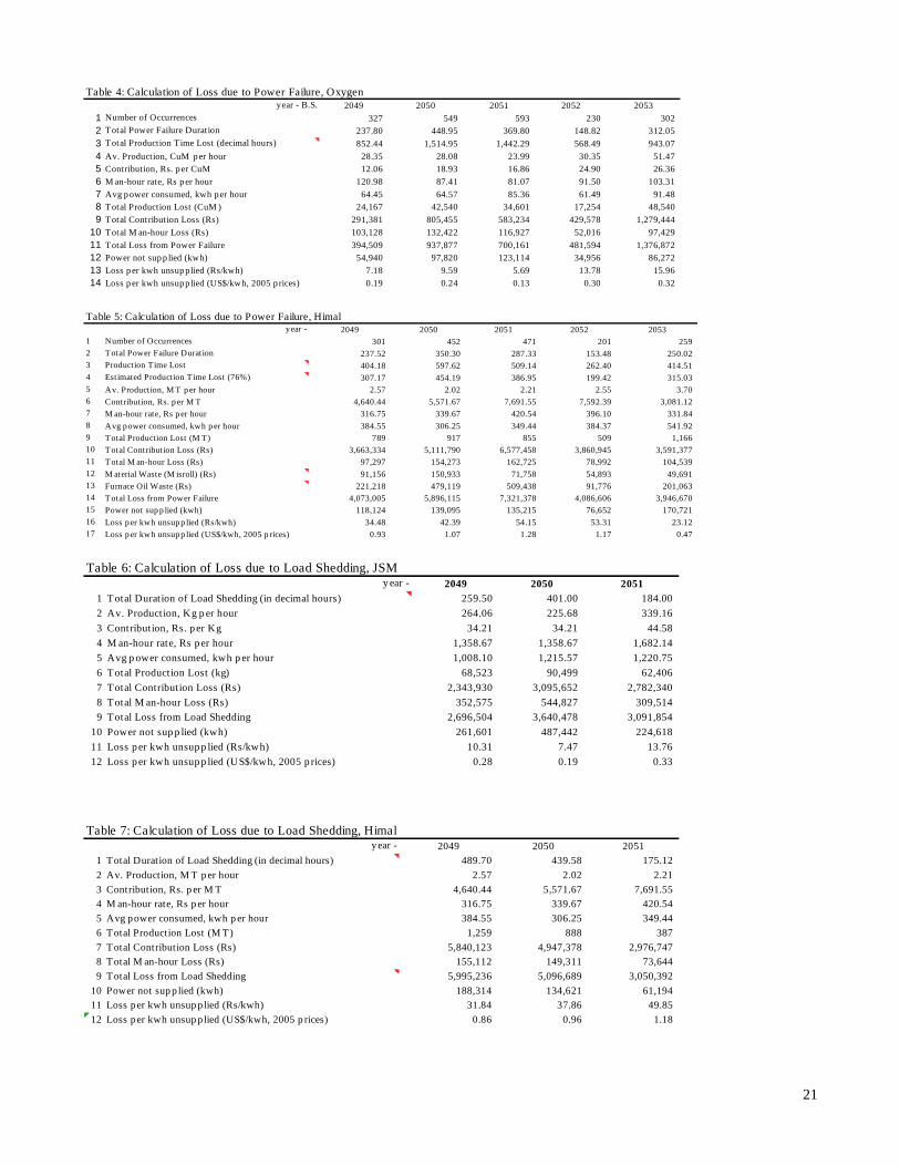
(insert Table 4)
For Oxygen the loss per kWh unsupplied in US$/kWh (2005 prices) ranged from US$ 0.13 to US$
0.32, with an average of US$ 0.24/kWh.
4 Workers cannot be sent home at a short notice or for the duration of the power failure. When we use the contribution method, we assume that the direct labor is saved but it is not. So, we need to add the cost of idle labor or the man-hours lost during the period of a power failure as a component of the cost. Idle direct labor rate is determined by dividing the total expenditure on direct labor by the total number of hours worked, in a particular year.

11
4.3.3 Losses from Power Failures at Himal
At Himal, the operating hours are from 6 AM to 10 PM, 6 AM to 2 PM for the first shift and from 2 PM
to 10 PM for the second shift. Hence all power outages occurring between 10 PM and 6 AM are
removed from the data. Furthermore, the power failures in 88 non-working days in the year are also
removed. Using equation (9) to translate each power failure duration into its impact on production time
lost, the total estimated production time lost from these power failures is 307.17 hours of production
time (Table 5 row 4).
On the basis of average production, contribution, and man-hour rate, total production loss, total
contribution loss and total man-hour loss are calculated, as in the case of JSM. At Himal, power
failures also result in wastage of the materials-in-process and the fuel oil, and these have to be
included. Himal kept records of the quantities of this wastage. Records are also available on the
selling price of the finished products and the purchase price of furnace oil in the respective years.
From these the value of the wastage is calculated. The furnace oil waste is a product of the quantity
and the price. In the case of material waste (misroll), an estimated cost equal to 50% of the regular
selling price of the final product gives us a reasonable approximation of the value of the input
materials wasted.
The total loss from power failures at Himal is the sum of the total contribution loss, the total man-hour
loss, the material waste, and the furnace oil waste. The loss per kWh unsupplied, is calculated as in
the case of JSM. The calculation of the losses per kWh are presented in Table 5.
(insert Table 5)
In the case of Himal the range of costs per US$/kWh is from US$ 0.47 to 1.28/kWh with a simple
average cost for these years of US$ 0.98/kWh.

12
Comparing the loss from power failures to the total contribution to profits of JSM we see that the loss
is only 1.57% of the total contribution from production that year. This is no doubt due to the fact that
JSM has its own electricity substation that has greatly reduced the incidence of power failures.
In the case of Oxygen, these numbers were higher. The power failure losses amounted to between
11.40% to a staggering 75.56% of total contribution from the annual production averaging 35.69%
over the five year period. At Himal, the losses were similarly high averaging 13.16% of the total
contribution from annual production over this period.
4.4 Calculation of the Cost of Load Shedding at the Three Enterprises
At JSM and Himal, the duration of the load shedding generally ranges from 1 to 3 hours, and so, the
workers cannot be sent home during the period of load shedding. Therefore, we must count the cost of
idle labor.
Because of the planned nature of load shedding the extra production time lost is relatively small as
compared to power failures. Hence, we will not apply the regression equation in this case to move
from the time of outage to the duration of lost production. From Table 2 we see that in B.S. 2049, we
see that at JSM a total of 259.50 hours of load shedding took place. The total production lost on
account of this was 68,523 kgs, and the contribution loss was Rs 2,343,930. Total idle labor cost of
the load shedding in this year was Rs 352,575 making the total loss from load shedding as Rs
2,696,504. The quantity of power not supplied during the periods of load shedding was 261,601 units
(kWh), hence, the loss per kWh not supplied was Rs 10.31 per kWh.
(insert Table 6)
(insert Table 7)

13
Due to the production process the situation at Oxygen is different. The interruption of electricity
whether planned or unplanned has a similar effect on extending the time of production loss beyond the
period of the power outage. We have, therefore, to take recourse to the regression equation (10)
derived earlier. The total impact of load shedding at Oxygen in B.S. 2049 is 706.72 hours (Table 8).
The remaining calculations are same as in the case of JSM and Himal.
(insert Table 8)
In Table 9 we calculate the opportunity cost of power failures and load shedding for these three
enterprises. Overall we find that for these three enterprises the values for power failures and load
shedding are very similar.
(insert Table 9)
5. Policy Implications
The outage data showed that the power supply in Nepal was very erratic and unreliable. Creating
standby self-generation capacity is the traditional solution for power supply problems but from our
analysis of outage data, another unique option has emerged – that of allowing the private ownership
and/or management of electricity substations.
5.1 Opportunity Cost of Power Supply for Outage Prevention
The value of the contribution lost per kWh not supplied is a measure of the opportunity cost of
marginal power supply for an enterprise. In other words, this would be the value of the willingness to
pay by these enterprises for the supply of power which would prevent such outages. Himal has the
highest opportunity cost of power in comparison to the other two. For the enterprise with higher
opportunity cost of power, it is more essential and feasible to invest in mitigating equipment.

14
5.2 Opportunity Cost of Uninterrupted Power Supply
We now calculate the opportunity cost of the electricity not supplied due to all types of power outages
during this period. To do this we calculate the levelized cost of the electricity lost (Table 10). The
levelized cost is obtained by taking the present value of the losses borne by each of the firms over the
five years and dividing this value by the present value of the quantity of the electricity supply lost
during this period. This is the rate of tariff that would make the NPV of the electricity not supplied equal
to the costs inflicted by the power outages. We see that this value is 0.23 US$/kWh for JSM, 0.21
US$/kWh for Oxygen and 0.95 US$/kWh for Himal!
(insert Table 10)
(insert Table 11)
(insert Table 12)
5.3 Evaluation of the Benefits and Costs of Privatizing Substation
The outages in power supply from a captive substation are considerably less than those from a
government owned NEA substation. Therefore, having a captive substation emerges as an option for
dealing with the power failure problem. The benefits associated with a captive substation are the
savings in power outage losses and the savings in buying high voltage power at a lower tariff than the
tariff charged for low voltage electric energy.
Using the data for JSM we are able to evaluate the option of having a captive substation (Table 13).
The savings obtained from purchasing high voltage electricity (row 13) is found by multiplying the
difference in the average tariff between purchasing low voltage versus high voltage electricity (row 12)
by the amount of power consumption (row 9). We calculate the saving in power outage losses (row 8)
by multiplying the levelized cost of outages (row 7) by the additional power supplied (row 6) because
these power failures have not occurred. This quantity of electricity estimated by comparing the higher

15
incidence (in hours) of power failures inflicted on Himal and those experienced by JSM. Recall Himal
and JSM are getting electricity from the same high voltage service but only JSM has its own
substation.
The costs associated with the captive substation are the annual capital cost and running cost. The
investment cost of the substation at the time of its purchase was US$ 647,000 in 2005 prices and the
operating costs have been about US$ 9,105 per year (2005 prices). Using a real (net of inflation) user
cost of capital of 15%, the annual capital cost is US$ 97,008.90, and the running cost is US$
9,105.005. This means that the annualized costs of operating a new substation is US$ 106,113.90,
Table 13 row 18. If we now compare this cost with the benefits it would produce through reducing the
electricity shortages (row 14), the results are striking.
(insert Table 13)
On average over these five years the combined benefits to JSM of purchasing the lower voltage power
plus the savings from the avoidance of the power failures covered the annual capital and operating
cost of the substation 2.18 times. The differential in the tariff rates for low and high voltage electricity
alone (row 13) covered the cost of the substation (row 18) in all years. In addition to this benefit, the
value of the reduced power failures to JSM (row 8) would alone on average cover, cover over 70% of
the annual capital and operating costs of the substation.
At the rates of levelized cost inflicted by power failures for these three enterprises it is clear that, if the
volume of electricity demanded is sufficient, an investment in one’s own substation is a very good
investment. In cases when a single firm’s consumption of electricity is not sufficient to justify the
purchase of a substation then it would be advantageous for enterprises to come together collectively
5 The capital costs of the substation and its operating costs were obtained from the financial records of JSM. The 15% user cost of capital is made up of a real opportunity cost of capital of 10% plus a 5% charge per year to reflect the depreciation of the investment of a substation with a 20 years economic life.

16
to purchase their own private substation. Other options might also be considered for getting private
management and incentives for proper management into this sector.
The fundamental reason for lower rate of power failures in electricity supply from one’s only substation
is good management of the substation. The NEA employees have little or no motivation to manage the
substations properly. The result is poor maintenance of the equipment and lack of proper
management practices. Leasing the substations to private operators who would buy the high voltage
power and sell the electricity to the private businesses might be another option for consideration.
Privatization of the substations can also result in another substantial benefit to the national economy.
In Nepal, as in several other countries in the region, pilferage of electricity is a serious problem.
Electricity is stolen by illegally tapping from the transmission lines and this happens only at the
secondary distribution voltage (220 V, single phase or 380 V, three phase). In other words, the
pilferage takes place after the substation. If the substation is privatized, NEA would collect payments
for electricity drawn at the substation. The private managers would be left to deal with the pilferage. It
is not difficult to identify where the pilferage is taking place, but NEA employees have no incentive for
doing this. Under private management, the situation would be different with the substation managers
having a very strong incentive to charge for every kWh of electricity supplied.
5.4 New Investment in Additional Capacity
If we subtract out the hours of lost electricity supply due to substation failures we have left the system
losses due to insufficient electricity generation capacity and other supply breakdowns. To simplify the
analysis we assume that all the rest of the power outages are caused by inadequate generation
capacity. This is the case certainly during the periods of planned load shedding, but most of the other
high voltage outages are likely to have risen due to a lack of generation capacity. This problem of lack
of reserve capacity can be addressed by NEA investing in additional generation capacity.

17
We now do a similar annualized cost benefit analysis to evaluate the benefits and costs of investing in
additional generation capacity. For the 5-year period, the levelized cost of power outages is US$
0.23/kWh for JSM, US$ 0.21 /kWh for Oxygen and US$ 0.95 /kWh for Himal. From the electricity lost
due to inadequate reserve capacity figures (Table 14), we found that 60% of the lost electricity
consumption was from JSM, 14% by Oxygen, and 26% by Himal. Using these percentages as the
weights, and taking the levelized costs for JSM, Oxygen, and Himal from tables 10, 11, and 12,
respectively we find that the weighted average levelized cost of the power not supplied is calculated to
be US$ 0.41/kWh.
(insert Table 14)
In 2005 prices, the cost of generation capacity suitable for supply power during peak load period is
approximately US$400 per kW.6 Assuming a 15% user cost of capital (10% opportunity cost of capital,
and 5% depreciation), the required contribution to the capital costs for a $400/kW investment in a gas
turbine generation would be $60/year. The running cost of such a plant are likely to be not more than
US$ 0.07/kWh. Given the number of hours system power outages, Table 15 row 5, we can estimate
the annual cost per year of having an additional kW of capacity. That is found by multiplying the
number of outage hours by the marginal running costs and adding the capital costs. These values are
reported in Table 15 rows 8, 9, 10.
The costs saved from having additional generation capacity in the system is found by multiplying the
levelized opportunity cost of US$ 0.41/kWh by hours per year when the power was not being supplied
(row 5). The total costs saved are reported in row 11. The benefit cost ratios for these years are
presented in Table 15 row 12.
6 The costs of such a reserve plant were obtained from Jenkins, Glenn and Andrey Klevchuk, Feasibility study of El-KureimatCombined Cycle Power Plant, African Development Bank, 1995 (www.queensjdiexec.org)
18
(insert Table 15)
From the annual benefit cost ratios we see that additional generation capacity was more than justified
during the first three years of this period 2049 to 2051. At this time there was systematic planned load
shedding. During 2052 and 2053 after additional generation capacity was bought into supply we find
the benefit cost ratio falls below one. It would appear that at least for these firms additional generation
capacity would not be justified during the two final years of observation7.
In contrast the problem of unexpected power failure due to inadequate capacity and management of
the substations would justify such investments throughout the entire five year period, Table 13 row 19.
6 Conclusion
We have seen that the uncertainties in power supply in Nepal pose serious threats to the economic
well being of the enterprises in that country. The opportunity costs range to as high as US$1.28/kWh
of electricity not supplied with a levelized average of US$ 0.41/kWh. In the past, installing generators
has been thought of as the only solution for the consumers to alleviate the power supply problem.
However, from the careful analysis of the data on power outages in Nepal, another mitigating strategy,
privatization of substations, emerges.
The issue of privatization is a common and popular topic of consideration in many developing
countries. In Nepal, the government and the donor agencies have been trying to motivate private
entrepreneurs to build hydropower stations to alleviate the power supply problems. Privatization of the
substations, however, is a complementary measure that in the short-run have much higher returns. In
addition, it is relatively easy to deal with either industrial groups or skilled entrepreneurs. In the case of
Nepal the return to an investor from ownership of a substation is potentially even higher than an
investment in additional generators to supply additional electricity. 7 The electricity system in Nepal is heavily dependent on electricity supplied by hydro dams. When there is a drought, load shedding is experienced. In 2005-2006 such a drought occurred causing a serious reduction in available electricity supplies and chronic load shedding. Hence, even if our results indicate that in the last two years of our study that additional electricity capacity was not justified, this situation might have only been temporary because of heavy rains in those years.

19
References
Beenstock, M., and E. Goldin (1997). “The Cost of Power Outages in the Business
and Public Sectors in Israel: Revealed Preference vs. Subjective Valuation.” The Energy Journal 18(2): 23-39. Bental, B. and S. Ravid (1982). “A Simple Method for Evaluating the Marginal Cost of Unsupplied Electricity.” Bell Journal of Economics 8(4): 249-253. Billington, R., and W. Wangdee (2005). “Approximate Methods for Event-Based Customer Interruption Cost Evaluation.” IEEE Transactions on Power Systems 20(2):1103:1110. Dahal, Madan K. and Kyoko Inoue (1994). A Profile of Industrial Development of Nepal. Tokyo Institute of Development Economics. Jenkins, Glenn and Andrey Klevchuk (2005). Feasibility study of El-Kureimat Combined Cycle Power Plant, African Development Bank. (www.queensjdiexec.org) Jyoti, Roop (1998). Investment Appraisal of Management Strategies for Addressing Uncertainties in Power Supply in the Context of Nepalese Manufacturing Enterprises. PhD dissertation, Harvard University, Cambridge, MA. Munasinghe, Mohan (1979). The Economics of Power System Reliability and Planning. Published for the World Bank, The John Hopkins University Press, Baltimore and London. Munasinghe, Mohan and Gellerson, Mark (1979). Optimum Economic Power Reliability, The World Bank, Washington. Nayak, Jit Narayan (1994). Science and Technology. Proceeding of IInd National Conference organized by Royal Nepal Academy of Science and Technology Kathmandu. Nexant SARI/Energy. October 2003. “Economic Impact of Poor Power Quality on Industry: Nepal.”
Perspective Energy Plan for Nepal (1995). [Volume 1: Summary], National Planning Commission Secretariat. Productivity improvement in Infrastructure, Productivity Tokyo, 1995. Swan, Neil M. (February 1, 1980). Economic Costs of Electricity Outages, Draft of Residential Sector Methodology, Mathtech, Inc, Princeton, New Jersey 08540.

20
Table1 : Frequency, Mean Duration and Cumulative Hours of Power Failure Per YearJSM Power Failure Summary (hours)
2049 2050 2051 2052 2053 Total AverageCount per year 40 125 101 107 57 430 86Mean length of occurrence 1.31 1.14 1.43 1.25 2.79 1.58Duration (hours per year) 52.20 142.12 144.60 134.13 158.83 631.88 126.38
Himal Power Failure Summary (hours)2049 2050 2051 2052 2053 Total Average
Count per year 327 549 593 230 302 2001 400.2Mean length of occurrence 0.73 0.82 0.62 0.65 1.03 0.8Duration (hours per year) 237.80 448.95 369.80 148.82 312.05 1517.42 303.5
Table 2: Frequency, Mean Duration and Cumulative Hours of Load Shedding Per YearJSM Load Shedding Summary (hours)
2049 2050 2051 2052 2053 Total AverageCount per year 108 203 92 403 134.33Mean length of occurrence 2.40 1.98 2.00 2.13Duration (hours per year) 259.50 401.00 184.00 844.50 281.50
Himal Load Shedding Summary (hours)2049 2050 2051 2052 2053 Total Average
Count per year 195 245 92 532 177.33Mean length of occurrence 3.00 1.90 1.91 2.27Duration (hours per year) 585.45 464.92 175.45 1225.82 408.61
Table 3: Calculation of Loss due to Power Failure, JSMy ear - B.S. 2049 2050 2051 2052 2053
1 Number of Occurrences 40 125 101 107 57 2 T otal Power Failure Duration 52.20 142.12 144.60 134.13 158.83 3 T otal Production Time Lost (decimal hours) 78.98 226.61 211.73 205.98 193.75 4 Av. Production, Kg p er hour 264.06 225.68 339.16 479.41 525.48 5 Contribution, Rs. per Kg 34.21 34.21 44.58 13.99 41.30 6 M an-hour rate, Rs p er hour 1,358.67 1,358.67 1,682.14 2,884.95 3,192.75 7 Avg power consumed, kwh p er hour 1,008.10 1,215.57 1,220.75 1,915.55 2,116.09 8 T otal Production Lost (kg) 20,855 51,141 71,810 98,748 101,814 9 T otal Contribution Loss (Rs) 713,376 1,749,368 3,201,596 1,381,163 4,204,516
10 T otal M an-hour Loss (Rs) 107,306 307,884 356,153 594,237 618,604 11 T otal Loss from Power Failure 820,683 2,057,252 3,557,749 1,975,400 4,823,119 12 Power not sup p lied (kwh) 79,618 275,456 258,464 394,561 409,998 13 Loss p er kwh unsup p lied (Rs/kwh) 10.31 7.47 13.76 5.01 11.76 14 Loss p er kwh unsup p lied (US$/kwh, 2005 p rices) 0.28 0.19 0.33 0.11 0.24
21
Table 4: Calculation of Loss due to Power Failure, Oxygeny ear - B.S. 2049 2050 2051 2052 2053
1 Number of Occurrences 327 549 593 230 302 2 Total Power Failure Duration 237.80 448.95 369.80 148.82 312.05 3 Total Production Time Lost (decimal hours) 852.44 1,514.95 1,442.29 568.49 943.07 4 Av. Production, CuM p er hour 28.35 28.08 23.99 30.35 51.47 5 Contribution, Rs. p er CuM 12.06 18.93 16.86 24.90 26.36 6 M an-hour rate, Rs p er hour 120.98 87.41 81.07 91.50 103.31 7 Avg p ower consumed, kwh p er hour 64.45 64.57 85.36 61.49 91.48 8 Total Production Lost (CuM ) 24,167 42,540 34,601 17,254 48,540 9 Total Contribution Loss (Rs) 291,381 805,455 583,234 429,578 1,279,444
10 Total M an-hour Loss (Rs) 103,128 132,422 116,927 52,016 97,429 11 Total Loss from Power Failure 394,509 937,877 700,161 481,594 1,376,872 12 Power not sup p lied (kwh) 54,940 97,820 123,114 34,956 86,272 13 Loss p er kwh unsup p lied (Rs/kwh) 7.18 9.59 5.69 13.78 15.96 14 Loss p er kwh unsup p lied (US$/kwh, 2005 p rices) 0.19 0.24 0.13 0.30 0.32
Table 5: Calculation of Loss due to Power Failure, Himalyear - 2049 2050 2051 2052 2053
1 Number of Occurrences 301 452 471 201 259 2 T otal Power Failure Duration 237.52 350.30 287.33 153.48 250.02 3 Production Time Lost 404.18 597.62 509.14 262.40 414.51 4 Estimated Production T ime Lost (76%) 307.17 454.19 386.95 199.42 315.03 5 Av. Production, M T p er hour 2.57 2.02 2.21 2.55 3.70 6 Contribution, Rs. p er M T 4,640.44 5,571.67 7,691.55 7,592.39 3,081.12 7 M an-hour rate, Rs p er hour 316.75 339.67 420.54 396.10 331.84 8 Avg power consumed, kwh p er hour 384.55 306.25 349.44 384.37 541.92 9 T otal Production Lost (M T) 789 917 855 509 1,166 10 T otal Contribution Loss (Rs) 3,663,334 5,111,790 6,577,458 3,860,945 3,591,377 11 T otal M an-hour Loss (Rs) 97,297 154,273 162,725 78,992 104,539 12 M aterial Waste (M isroll) (Rs) 91,156 150,933 71,758 54,893 49,691 13 Furnace Oil Waste (Rs) 221,218 479,119 509,438 91,776 201,063 14 T otal Loss from Power Failure 4,073,005 5,896,115 7,321,378 4,086,606 3,946,670 15 Power not sup p lied (kwh) 118,124 139,095 135,215 76,652 170,721 16 Loss p er kwh unsup p lied (Rs/kwh) 34.48 42.39 54.15 53.31 23.12 17 Loss p er kwh unsup p lied (US$/kwh, 2005 p rices) 0.93 1.07 1.28 1.17 0.47
Table 6: Calculation of Loss due to Load Shedding, JSMy ear - 2049 2050 2051
1 Total Duration of Load Shedding (in decimal hours) 259.50 401.00 184.00 2 Av. Production, Kg p er hour 264.06 225.68 339.16 3 Contribution, Rs. p er Kg 34.21 34.21 44.58 4 M an-hour rate, Rs p er hour 1,358.67 1,358.67 1,682.14 5 Avg p ower consumed, kwh p er hour 1,008.10 1,215.57 1,220.75 6 Total Production Lost (kg) 68,523 90,499 62,406 7 Total Contribution Loss (Rs) 2,343,930 3,095,652 2,782,340 8 Total M an-hour Loss (Rs) 352,575 544,827 309,514 9 Total Loss from Load Shedding 2,696,504 3,640,478 3,091,854
10 Power not sup p lied (kwh) 261,601 487,442 224,618 11 Loss p er kwh unsup p lied (Rs/kwh) 10.31 7.47 13.76 12 Loss p er kwh unsup p lied (US$/kwh, 2005 p rices) 0.28 0.19 0.33
Table 7: Calculation of Loss due to Load Shedding, Himalyear - 2049 2050 2051
1 Total Duration of Load Shedding (in decimal hours) 489.70 439.58 175.12 2 Av. Production, M T p er hour 2.57 2.02 2.21 3 Contribution, Rs. p er M T 4,640.44 5,571.67 7,691.55 4 M an-hour rate, Rs p er hour 316.75 339.67 420.54 5 Avg power consumed, kwh p er hour 384.55 306.25 349.44 6 Total Production Lost (M T) 1,259 888 387 7 Total Contribution Loss (Rs) 5,840,123 4,947,378 2,976,747 8 Total M an-hour Loss (Rs) 155,112 149,311 73,644 9 Total Loss from Load Shedding 5,995,236 5,096,689 3,050,392
10 Power not sup p lied (kwh) 188,314 134,621 61,194 11 Loss per kwh unsup p lied (Rs/kwh) 31.84 37.86 49.85 12 Loss per kwh unsup p lied (US$/kwh, 2005 p rices) 0.86 0.96 1.18

22
Table 8: Calculation of Loss due to Load Shedding, Oxygenyear - 2049 2050 2051
1 Number of Occurrences 195 245 92 2 Total Power Failure Duration 259.50 401.00 184.00 3 Total Impact of Load Shedding (in decimal hours) 706.72 1,014.29 437.21 4 Av. Production, CuM per hour 28.35 28.08 23.99 5 Contribution, Rs. p er CuM 12.06 18.93 16.86 6 M an-hour rate, Rs per hour 120.98 87.41 81.07 7 Avg power consumed, kwh p er hour 64.45 64.57 85.36 8 Total Production Lost (CuM ) 20,036 28,481 10,489 9 Total Contribution Loss (Rs) 241,572 539,271 176,799
10 Total M an-hour Loss (Rs) 85,499 88,659 35,445 11 Total Loss from Load Shedding 327,072 627,930 212,244 12 Power not sup p lied (kwh) 45,548 65,493 37,320 13 Loss p er kwh unsupp lied (Rs/kwh) 7.18 9.59 5.69 14 Loss p er kwh unsupp lied (US$/kwh, 2005 p rices) 0.19 0.24 0.13
y ear 2049 2050 2051 2052 2053
JSM 0.28 0.19 0.33 0.11 0.24Oxy gen 0.19 0.24 0.13 0.30 0.32
Himal 0.93 1.07 1.28 1.17 0.47
JSM 0.28 0.19 0.33 -- --Oxy gen 0.19 0.24 0.13 -- --
Himal 0.93 1.07 1.28 -- --
Power Failure
Load S hedding
Table 9: Op p ortunity Cost of Power Failures and Load Shedding, US$/kWh, 2005
Table 10: Levelized Cost of Power Outages, JSM y ear > 2049 2050 2051 2052 2053
1 Total Costs (2049 p rices) 3,517,187 5,304,283 5,805,187 1,600,081 3,608,596 2 Quantity of kWhs not Sup p lied 341,219 762,898 483,082 394,561 409,998 3 Levelized cost (Rs/kWh, 2049 p rices) 8.36 4 Levelized Cost (US$/kWh, 2005 p rices) 0.23
Table 11: Levelized Cost of Power Outages, Oxygenyear > 2049 2050 2051 2052 2053
1 Total Costs (2049 p rices) 721,580.45 1,457,682.37 796,540.77 390,092.93 1,030,158.27 2 Quantity of kWhs not Supp lied 100,488 163,313 160,435 34,956 86,272 3 Levelized cost (Rs/kWh, 2049 p rices) 7.934 Levelized Cost (US$/kWh, 2005 p rices) 0.21
Table 12: Levelized Cost of Power Outages, Himal y ear > 2049 2050 2051 2052 2053
1 Total Costs (2049 p rices) 10,068,241 10,233,714 9,054,686 3,310,164 2,952,848 2 Quantity of kWhs not Supp lied 306,438 273,717 196,409 76,652 170,721 3 Levelized cost (Rs/kWh, 2049 p rices) 35.164 Levelized Cost (US$/kWh, 2005 p rices) 0.95

23
Table 13: Cost/Benefit Analysis of S ubstationyear > 2049 2050 2051 2052 2053
1 Duration of p ower outages (hrs)2 without substation 823.25 913.87 545.25 185.57 312.05 3 with substat ion 311.70 543.12 328.60 134.13 158.83 4 Difference 511.55 370.75 216.65 51.43 153.22
5 Avg p ower consumed, kwh p er hour 1,008.10 1,215.57 1,220.75 1,915.55 2,116.09 6 Additional Power sup p lied (kWh) 515,691.66 450,671.36 264,475.39 98,522.98 324,220.39
7 Levelized Cost of Power Outages (US$/kWh, 2005 p ri 0.23 8 Saving in p ower outage losses 116,801.22 102,074.50 59,902.17 22,314.89 73,434.07
9 Power consump tion (kWh) 14,050,805.00 9,123,436.00 10,345,670.00 14,412,578.00 15,545,502.00
10 Average tariff (11 kV, US$ 2005 p rices) 0.05 0.06 0.07 0.06 0.07 11 Average tariff (66 kV, US$ 2005 p rices) 0.04 0.05 0.06 0.05 0.05 12 Difference 0.01 0.01 0.01 0.01 0.01 13 Saving in tariff rate 123,746.60 107,133.86 149,570.66 187,062.47 212,234.72
14 T otal Savings 240,547.82 209,208.35 209,472.83 209,377.37 285,668.79
15 Cost of Cap tive Substation16 Cap ital cost 97,008.90 97,008.90 97,008.90 97,008.90 97,008.90 17 Running cost 9,105.00 9,105.00 9,105.00 9,105.00 9,105.00 18 Total Cost of Cap tive Substat ion (US$) 106,113.90 106,113.90 106,113.90 106,113.90 106,113.90
19 Ratio of Benefits to Substation cost 2.27 1.97 1.97 1.97 2.69 20 Annual Average 2.18
Table 14: Electricity lost kWh/year due to inadequate reserve capaci tyyear > 2049 2050 2051 2052 2053 Total Units Weights
JSM 341,219.41 762,898.26 483,082.34 394,561.01 409,998.20 2,391,759.23 0.60 Oxygen 100,487.88 163,312.91 160,434.52 34,956.17 86,272.09 545,463.56 0.14 Him al 306,437.95 273,716.51 196,408.81 76,652.19 170,720.69 1,023,936.15 0.26
Table 15: Cost/Benefit Analysis of Additional Generation Capacity1 year > 2049 2050 2051 2052 20532 Duration of Power Outages (hours)3 Power Failures 52.20 142.12 144.60 134.13 158.83 4 Load Shedding 259.50 401.00 184.00 - - 5 Total Power Outage Duration (hours) 311.70 543.12 328.60 134.13 158.83
6 Levelized Cost of Power Outages (US$/kWh, 2005 p rices)7 (US$/kWh, 2005 p rices) 0.41 0.41 0.41 0.41 0.41
8 Running Cost of Generat ion 21.82 38.02 23.00 9.39 11.12 9 Cap ital cost 60.00 60.00 60.00 60.00 60.00
10 T otal Annual Costs 81.82 98.02 83.00 69.39 71.12 11 Costs Saved 127.80 222.68 134.73 54.99 65.12 12 Ratio of outage cost to cap acity cost 1.56 2.27 1.62 0.79 0.92 13 Annual Average 1.43
