NASA/CR{2001{210849

Inviscid Flow Computations of theOrbital Sciences X-34 Over a MachNumber Range of 1.25 to 6.0

Ramadas K. Prabhu

Lockheed Martin Engineering & Sciences Company, Hampton, Virginia

April 2001

The NASA STI Program O�ce ... in Pro�le

Since its founding, NASA has been dedicatedto the advancement of aeronautics and spacescience. The NASA Scienti�c and TechnicalInformation (STI) Program O�ce plays a keypart in helping NASA maintain thisimportant role.

The NASA STI Program O�ce is operated byLangley Research Center, the lead center forNASA's scienti�c and technical information.The NASA STI Program O�ce providesaccess to the NASA STI Database, thelargest collection of aeronautical and spacescience STI in the world. The Program O�ceis also NASA's institutional mechanism fordisseminating the results of its research anddevelopment activities. These results arepublished by NASA in the NASA STI ReportSeries, which includes the following reporttypes:

� TECHNICAL PUBLICATION. Reports ofcompleted research or a major signi�cantphase of research that present the resultsof NASA programs and include extensivedata or theoretical analysis. Includescompilations of signi�cant scienti�c andtechnical data and information deemedto be of continuing reference value. NASAcounterpart of peer-reviewed formalprofessional papers, but having lessstringent limitations on manuscriptlength and extent of graphicpresentations.

� TECHNICAL MEMORANDUM.Scienti�c and technical �ndings that arepreliminary or of specialized interest,e.g., quick release reports, workingpapers, and bibliographies that containminimal annotation. Does not containextensive analysis.

� CONTRACTOR REPORT. Scienti�c andtechnical �ndings by NASA-sponsoredcontractors and grantees.

� CONFERENCE PUBLICATION.Collected papers from scienti�c andtechnical conferences, symposia,seminars, or other meetings sponsored orcosponsored by NASA.

� SPECIAL PUBLICATION. Scienti�c,technical, or historical information fromNASA programs, projects, and missions,often concerned with subjects havingsubstantial public interest.

� TECHNICAL TRANSLATION. English-language translations of foreign scienti�cand technical material pertinent toNASA's mission.

Specialized services that help round out theSTI Program O�ce's diverse o�erings includecreating custom thesauri, building customizeddatabases, organizing and publishingresearch results. . . even providing videos.

For more information about the NASA STIProgram O�ce, see the following:

� Access the NASA STI Program HomePage at http://www.sti.nasa.gov

� E-mail your question via the Internet tohelp@sti.nasa.gov

� Fax your question to the NASA STIHelp Desk at (301) 621{0134

� Phone the NASA STI Help Desk at(301) 621{0390

� Write to:NASA STI Help DeskNASA Center for AeroSpace Information7121 Standard DriveHanover, MD 21076{1320

NASA/CR{2001{210849

Inviscid Flow Computations of theOrbital Sciences X-34 Over a MachNumber Range of 1.25 to 6.0

Ramadas K. Prabhu

Lockheed Martin Engineering & Sciences Company, Hampton, Virginia

National Aeronautics andSpace Administration

Langley Research Center Prepared for Langley Reseach Center

Hampton, Virginia 23681{2199 under contract NAS1-96014

April 2001

Available from the following:

NASA Center for AeroSpace Information (CASI) National Technical Information Service (NTIS)

7121 Standard Drive 5285 Port Royal Road

Hanover, MD 21076{1320 Spring�eld, VA 22161{2171

(301) 621{0390 (703) 487{4650

Summary

This report documents the results of a computational study conducted to compute the inviscid longitudinalaerodynamic characteristics of the Orbital Sciences X-34 vehicle over a Mach number range of 1.25 to 6.0. Theunstructured grid software FELISA was used and the aerodynamic characteristics were computed for Machnumbers of 1.25, 1.6, 2.5, 4.0, 4.63, and 6.0, over an angle of attack range of -4 to 32 degrees. These resultswere compared with available aerodynamic data from wind tunnel tests on X-34 models. The comparisonshowed very good agreement in normal force coe�cients over the entire Mach number and angle of attackranges. The computed pitching moment coe�cients compared well at Mach numbers 2.5 and above, and atangles of attack of up to 12 deg. The agreement was not good at higher angles of attack possibly due toviscous e�ects. At lower Mach numbers (1.6 and 1.25) there were signi�cant di�erences between computedand measured pitching moment coe�cient values; this is also attributed to viscous e�ects. Since the presentcomputations are inviscid, the computed axial force coe�cients were consistently lower than the measuredvalues as expected.

Nomenclature

CA Axial force coe�cient

CN Normal force coe�cient

Cm Pitching moment coe�cient about the point ( 0.877, 0, -14.0 )

Cp (p - p1)/q1, Pressure coe�cient

lref Reference length for pitching moment ( =5.8167 in.)

M1 Freestream Mach number

p1

Freestream static pressure

q1

p1M2

1/2, Freestream dynamic pressure

Sref Reference area ( =27.2 sq. in. )

x, y, z Cartesian co-ordinates of a given point; (The origin is at the nose, with the x-axisin the vertical direction, the y-axis in the spanwise direction, and the z-axis in theaxial direction pointing into the stream.)

� Angle of attack, deg.

Ratio of speci�c heats

Introduction

In a study aimed at providing new space-transportation systems to replace the aging space shuttle, NASA hadrecommended [1] the development of fully reusable, single-stage-to-orbit concepts. The major requirementsfor such space transportation systems are low-cost and reliable operations. The X-34 is an industry ledprogram jointly funded by the industry and the Government to develop cheaper and reliable single-stage-to-orbit technology. The X-34 is a Reusable Launch Vehicle (RLV) designed to insert relatively small (1000 -2000lb.) payloads into earth orbit.

The unmanned rocket powered X-34 RLV would be air launched from a Lockheed L-1011 aircraft ata Mach number of 0.7. After the separation, the liquid rocket motor would �re, and the vehicle wouldaccelerate to sub-orbital speed and reach an altitude of approximately 300,000 ft. At this point the payload

1

with attached upper stage motor would separate form the RLV. Next, the upper stage motor would �re,sending the payload into the required orbit. After releasing the upper stage, the X-34 reusable vehiclewould decelerate, descend, and eventually land on a conventional runway. In this industry/Governmentpartnership venture, Orbital Science Corporation is responsible for designing, building, and ight testing theX-34 vehicle. During the design process, the Aerothermodynamics Branch (AB), NASA Langley ResearchCenter provided much of the wind tunnel testing for the X-34 vehicle to determine the aerodynamic loadsand aero-heating at the ight conditions. In addition, AB also provided valuable CFD predictions of theaerodynamic and thermal loads on the X-34 vehicle.

Unstructured grid technology is known to provide quick and reliable CFD solutions to complex owproblems particularly for hypersonic ows. Among the widely used unstructured grid software packages arethe FELISA [2] and the TetrUSS [3] systems. In the Aerothermodynamics Branch, FELISA inviscid owsolvers have been used extensively for the prediction of ow over complex vehicles. These ow solvers, likeany other inviscid ow solvers, have obvious limitations; because of the absence of a boundary layer there isno skin friction and no ow separation e�ects. However, the inviscid ow solvers generally yield good normalforce and pitching moment results up to a point where the e�ects of ow separation are not signi�cant.

This paper presents the results of an inviscid computational study for the X-34 vehicle using the un-structured grid software FELISA. A Mach number range of 1.6{6.0 and an angle of attack range of -4{32 iscovered in the present study. The results are compared with the experimental data measured in wind tunneltests conducted on X-34 models in the NASA Langley wind tunnels.

The FELISA Software

All the computations of the present study were done using the unstructured grid software FELISA. Thissoftware package has proved to be a powerful tool for fast inviscid ow computations. It consists of a setof computer codes for the generation of unstructured grids of tetrahedral elements and the simulation ofthree-dimensional steady inviscid ows using these grids. Surface triangulation and discretization of thecomputational domain using tetrahedral elements are done by two separate codes. There are two owsolvers|one applicable for transonic ows and the other for hypersonic ows with an option for perfect gasair, equilibrium air, and CF4 gases. Both the solvers were used in the present study. Only the perfect gasoption with the speci�c heat ratio =1.4 was used. Post-processors like the aerodynamic analysis routineused in the study, are part of the FELISA software package. More information on FELISA may be found inreference [2].

Geometry

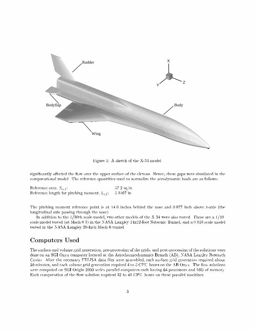
A 1/30th scale wind tunnel model of the X-34 was tested extensively over a Mach number of 0.4{4.63 inthe wind tunnels at NASA Langley Research Center. This model has all the major components of the X-34vehicle, namely, the body, the wing, the rudder, and the body ap. However, the engine bell was absenton the model; instead, there was a sting for the model support. This con�guration was reproduced in thecomputational model. A sketch of the X-34 vehicle is shown in Fig. 1. Since the con�guration has a planeof symmetry, only one half of the model was simulated in the computational study. The length of the modelfrom its nose to the base is 21.56 inches and the wing semi-span is 5.548 inches. The sting used to mount themodel (not shown in the �gure) in the wind tunnel test section has a diameter of 1.15 inches. Preliminarycomputations had indicated that the gaps between the two elevons and the inboard elevon and the body

2

X

YZ

Rudder

Body

Wing

Bodyflap

Figure 1: A sketch of the X-34 model.

signi�cantly a�ected the ow over the upper surface of the elevons. Hence, these gaps were simulated in thecomputational model. The reference quantities used to normalize the aerodynamic loads are as follows:

Reference area, Sref : 57.2 sq.in.Reference length for pitching moment, lref : 5.8167 in.

The pitching moment reference point is at 14.0 inches behind the nose and 0.877 inch above z-axis (thelongitudinal axis passing through the nose).

In addition to the 1/30th scale model, two other models of the X-34 were also tested. These are a 1/10-scale model tested (at Mach 0.3) in the NASA Langley 14x22-foot Subsonic Tunnel, and a 0.018 scale modeltested in the NASA Langley 20-Inch Mach 6 tunnel.

Computers Used

The surface and volume grid generation, pre-processing of the grids, and post-processing of the solutions weredone on an SGI Onyx computer located at the Aerothermodynamics Branch (AB), NASA Langley ResearchCenter. After the necessary FELISA data �les were assembled, each surface grid generation required about30 minutes, and each volume grid generation required 4 to 5 CPU hours on the AB Onyx. The ow solutionswere computed on SGI Origin 2000 series parallel computers each having 64 processors and 16G of memory.Each computation of the ow solution required 32 to 40 CPU hours on these parallel machines.

3

(a) Side view (b) Front view

Figure 2: Computational domain for Mach 1.25 and 1.6.

Grids

The geometrical information of the X-34 model was received in the form of an IGES �le. This was processedusing the software GridTool [4], and a set of FELISA data �les was generated. These data �les were used togenerate all the grids used in the present study.

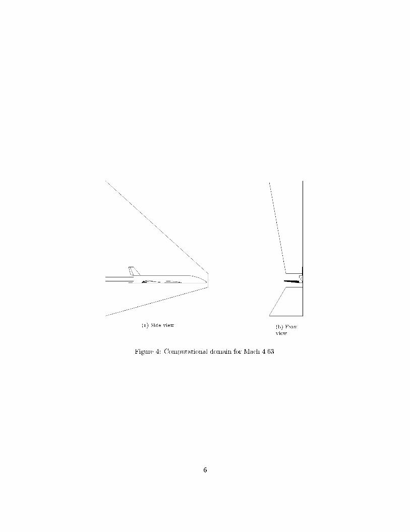
Four grids were used in the present study. The computational domains for these grids were chosen to besu�ciently large and away from the body so that except for the exit plane, all the boundary surfaces werein the freestream ow.

A single grid was used for the computations at Mach 1.25 and 1.60. The computational domain used forthis grid is shown in Fig. 2. The model surface triangulation for this is shown in Fig. 3. The support stingis present in the CFD model, but is not shown in this �gure. The unstructured tetrahedral grid (designatedgrid 1) for this case has 1,058,983 points. The minimum grid spacing was 0.0043 in. near the nose. The gridspacing near the wing leading edge varied from 0.012 in. at the tip 0.02 in. at the root.

A second grid was built for Mach number 2.5{6.0 computations. The computational domain chosen forthis grid is shown in Fig. 4, and the surface triangulation is shown in Figure 5. This grid (designated grid2) has 1,042,427 points, and a grid spacing of 0.063 in. over the wing upper surface.

Preliminary studies using grid 2 at Mach 2.5 indicated that there were complex ow features over thewing upper surface particularly at angles of attack greater than 8 deg. In order to better resolve these owfeatures, it was decided to re�ne the grid over the wing, and a third grid was built. This grid (designatedgrid 3) has the spacing over the wing reduced to 0.033 in. The spacing in other regions of the grid wereunaltered. This grid has 1,262,391 points.

4

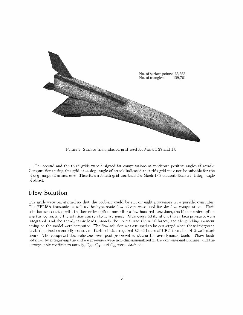
No. of surface points: 68,863No. of triangles: 139,761

Figure 3: Surface triangulation grid used for Mach 1.25 and 1.6.

The second and the third grids were designed for computations at moderate positive angles of attack.Computations using this grid at -4 deg. angle of attack indicated that this grid may not be suitable for the-4 deg. angle of attack case. Therefore a fourth grid was built for Mach 4.63 computations at -4 deg. angleof attack.

Flow Solution

The grids were partitioned so that the problem could be run on eight processors on a parallel computer.The FELISA transonic as well as the hypersonic ow solvers were used for the ow computations. Eachsolution was started with the low-order option, and after a few hundred iterations, the higher-order optionwas turned on, and the solution was run to convergence. After every 50 iteration, the surface pressures wereintegrated, and the aerodynamic loads, namely the normal and the axial forces, and the pitching momentacting on the model were computed. The ow solution was assumed to be converged when these integratedloads remained essentially constant. Each solution required 32{40 hours of CPU time, i.e., 4{5 wall clockhours. The computed ow solutions were post-processed to obtain the aerodynamic loads. These loadsobtained by integrating the surface pressures were non-dimensionalized in the conventional manner, and theaerodynamic coe�cients namely, CN , CA, and Cm were obtained.

5

(a) Side view (b) Frontview

Figure 4: Computational domain for Mach 4.63.

6

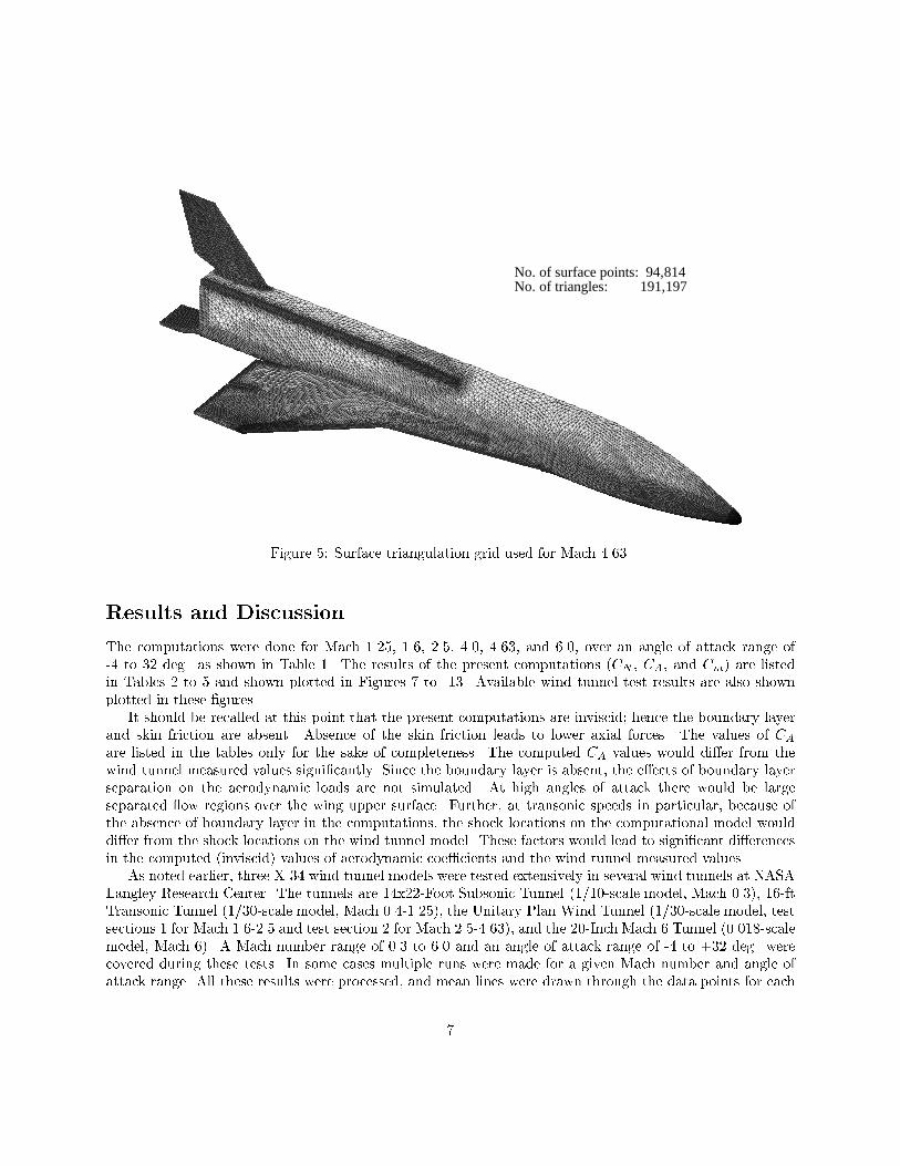
No. of surface points: 94,814No. of triangles: 191,197

Figure 5: Surface triangulation grid used for Mach 4.63.

Results and Discussion

The computations were done for Mach 1.25, 1.6, 2.5, 4.0, 4.63, and 6.0, over an angle of attack range of-4 to 32 deg. as shown in Table 1. The results of the present computations (CN , CA, and Cm) are listedin Tables 2 to 5 and shown plotted in Figures 7 to 13. Available wind tunnel test results are also shownplotted in these �gures.

It should be recalled at this point that the present computations are inviscid; hence the boundary layerand skin friction are absent. Absence of the skin friction leads to lower axial forces. The values of CAare listed in the tables only for the sake of completeness. The computed CA values would di�er from thewind tunnel measured values signi�cantly. Since the boundary layer is absent, the e�ects of boundary layerseparation on the aerodynamic loads are not simulated. At high angles of attack there would be largeseparated ow regions over the wing upper surface. Further, at transonic speeds in particular, because ofthe absence of boundary layer in the computations, the shock locations on the computational model woulddi�er from the shock locations on the wind tunnel model. These factors would lead to signi�cant di�erencesin the computed (inviscid) values of aerodynamic coe�cients and the wind tunnel measured values.

As noted earlier, three X-34 wind tunnel models were tested extensively in several wind tunnels at NASALangley Research Center. The tunnels are 14x22-Foot Subsonic Tunnel (1/10-scale model, Mach 0.3), 16-ftTransonic Tunnel (1/30-scale model, Mach 0.4-1.25), the Unitary Plan Wind Tunnel (1/30-scale model, testsections 1 for Mach 1.6-2.5 and test section 2 for Mach 2.5-4.63), and the 20-Inch Mach 6 Tunnel (0.018-scalemodel, Mach 6). A Mach number range of 0.3 to 6.0 and an angle of attack range of -4 to +32 deg. werecovered during these tests. In some cases multiple runs were made for a given Mach number and angle ofattack range. All these results were processed, and mean lines were drawn through the data points for each

7

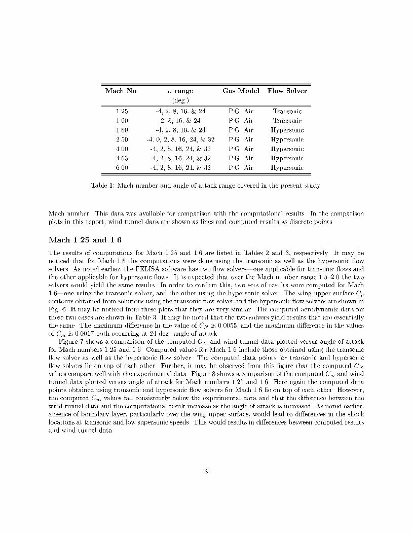
Mach No. � range Gas Model Flow Solver

(deg.)

1.25 -4, 2, 8, 16, & 24 P.G. Air Transonic

1.60 2, 8, 16, & 24 P.G. Air Transonic

1.60 -4, 2, 8, 16, & 24 P.G. Air Hypersonic

2.50 -4, 0, 2, 8, 16, 24, & 32 P.G. Air Hypersonic

4.00 -4, 2, 8, 16, 24, & 32 P.G. Air Hypersonic

4.63 -4, 2, 8, 16, 24, & 32 P.G. Air Hypersonic

6.00 -4, 2, 8, 16, 24, & 32 P.G. Air Hypersonic

Table 1: Mach number and angle of attack range covered in the present study.

Mach number. This data was available for comparison with the computational results. In the comparisonplots in this report, wind tunnel data are shown as lines and computed results as discrete points.

Mach 1.25 and 1.6

The results of computations for Mach 1.25 and 1.6 are listed in Tables 2 and 3, respectively. It may benoticed that for Mach 1.6 the computations were done using the transonic as well as the hypersonic owsolvers. As noted earlier, the FELISA software has two ow solvers|one applicable for transonic ows andthe other applicable for hypersonic ows. It is expected that over the Mach number range 1.5{2.0 the twosolvers would yield the same results. In order to con�rm this, two sets of results were computed for Mach1.6|one using the transonic solver, and the other using the hypersonic solver. The wing upper surface Cpcontours obtained from solutions using the transonic ow solver and the hypersonic ow solvers are shown inFig. 6. It may be noticed from these plots that they are very similar. The computed aerodynamic data forthese two cases are shown in Table 3. It may be noted that the two solvers yield results that are essentiallythe same. The maximum di�erence in the value of CN is 0.0055, and the maximum di�erence in the valuesof Cm is 0.0017 both occurring at 24 deg. angle of attack.

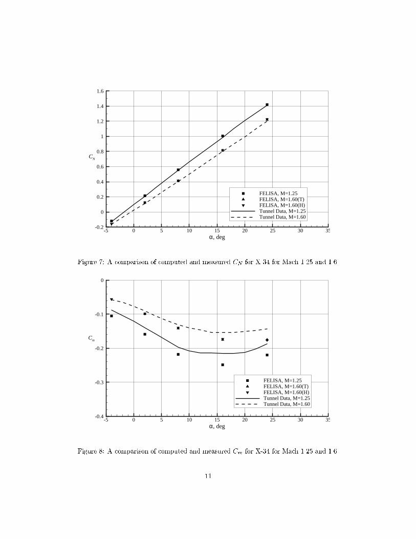
Figure 7 shows a comparison of the computed CN and wind tunnel data plotted versus angle of attackfor Mach numbers 1.25 and 1.6. Computed values for Mach 1.6 include those obtained using the transonic ow solver as well as the hypersonic ow solver. The computed data points for transonic and hypersonic ow solvers lie on top of each other. Further, it may be observed from this �gure that the computed CNvalues compare well with the experimental data. Figure 8 shows a comparison of the computed Cm and windtunnel data plotted versus angle of attack for Mach numbers 1.25 and 1.6. Here again the computed datapoints obtained using transonic and hypersonic ow solvers for Mach 1.6 lie on top of each other. However,the computed Cm values fall consistently below the experimental data and that the di�erence between thewind tunnel data and the computational result increase as the angle of attack is increased. As noted earlier,absence of boundary layer, particularly over the wing upper surface, would lead to di�erences in the shocklocations at transonic and low supersonic speeds. This would results in di�erences between computed resultsand wind tunnel data.

8

Mach No. � CN CA Cm Grid Flow Solver

(deg.)

1.25 -4 -0.1197 0.0842 -0.0924 Grid 1 Transonic

1.25 2 0.2144 0.0794 -0.1469 Grid 1 Transonic

1.25 8 0.5579 0.0696 -0.2075 Grid 1 Transonic

1.25 16 1.0054 0.0459 -0.2417 Grid 1 Transonic

1.25 24 1.4201 0.0283 -0.2156 Grid 1 Transonic

Table 2: Computed CN , CA, and Cm for X-34 for Mach 1.25

Mach No. � CN CA Cm Grid Flow Solver

(deg.)

1.60 2 0.1228 0.0684 -0.0889 Grid 1 Transonic

1.60 8 0.4099 0.0591 -0.1325 Grid 1 Transonic

1.60 16 0.8123 0.0428 -0.1684 Grid 1 Transonic

1.60 24 1.2215 0.0331 -0.1699 Grid 1 Transonic

1.60 -4 -0.1575 0.0696 -0.0454 Grid 1 Hypersonic

1.60 2 0.1261 0.0648 -0.0885 Grid 1 Hypersonic

1.60 8 0.4152 0.0557 -0.1315 Grid 1 Hypersonic

1.60 16 0.8174 0.0398 -0.1670 Grid 1 Hypersonic

1.60 24 1.2270 0.0304 -0.1716 Grid 1 Hypersonic

Table 3: Computed CN , CA, and Cm for X-34 for Mach 1.6 using the transonic and hypersonic ow solvers.

9

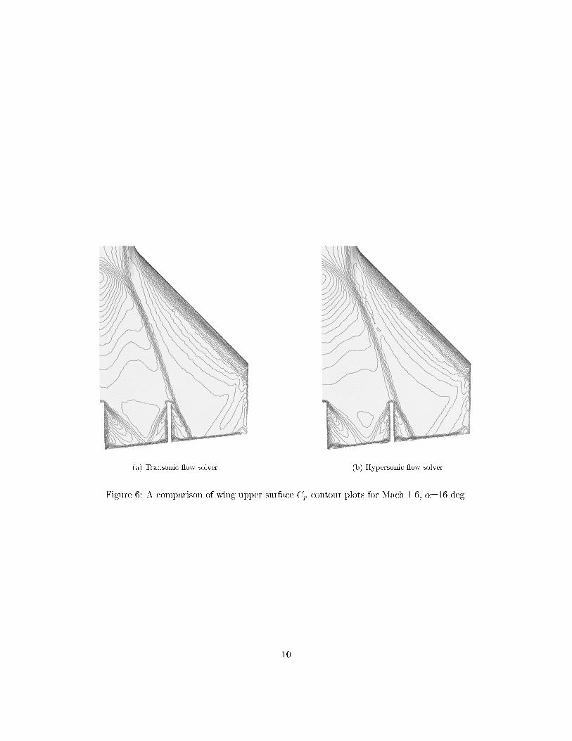
(a) Transonic ow solver (b) Hypersonic ow solver

Figure 6: A comparison of wing upper surface Cp contour plots for Mach 1.6, �=16 deg.

10

-5 0 5 10 15 20 25 30 35α, deg

-0.2

0

0.2

0.4

0.6

0.8

1

1.2

1.4

1.6

FELISA, M=1.25FELISA, M=1.60(T)FELISA, M=1.60(H)Tunnel Data, M=1.25Tunnel Data, M=1.60

CN

Figure 7: A comparison of computed and measured CN for X-34 for Mach 1.25 and 1.6.

-5 0 5 10 15 20 25 30 35α, deg

-0.4

-0.3

-0.2

-0.1

0

FELISA, M=1.25FELISA, M=1.60(T)FELISA, M=1.60(H)Tunnel Data, M=1.25Tunnel Data, M=1.60

Cm

Figure 8: A comparison of computed and measured Cm for X-34 for Mach 1.25 and 1.6.

11

Mach No. � CN CA Cm Grid Flow Solver

(deg.)

2.50 -4 -0.1449 0.0551 -0.0418 Grid 2 Hypersonic

2.50 2 0.0506 0.0489 -0.0465 Grid 2 Hypersonic

2.50 8 0.2569 0.0412 -0.0605 Grid 2 Hypersonic

2.50 16 0.5554 0.0324 -0.0734 Grid 2 Hypersonic

2.50 24 0.9055 0.0250 -0.0755 Grid 2 Hypersonic

2.50 32 1.2959 0.0178 -0.0798 Grid 2 Hypersonic

2.50 0 -0.0143 0.0514 -0.0437 Grid 3 Hypersonic

2.50 16 0.5562 0.0324 -0.0735 Grid 3 Hypersonic

2.50 24 0.9058 0.0249 -0.0753 Grid 3 Hypersonic

2.50 32 1.2964 0.0177 -0.0789 Grid 3 Hypersonic

Table 4: Computed CN , CA, and Cm for X-34 for Mach 4.0, 4.63, and 6.0

Mach 2.5

The computations for Mach 2.5 were done using two separate grids to determine the e�ect of grid re�nementon the results. The �rst set of computations was done using a grid designated as grid 2. This grid has agrid spacing of 0.063 in. over the wing upper surface. The next set of computations was done using a griddesignated grid 3. This grid has the spacing over the wing reduced to 0.033 in. The spacing in other regionsof the grid were unaltered. The wing upper surface Cp contours obtained from solutions using grids 2 and3 for � = 16 deg. are shown in Fig. 9. It may be noticed from these plots that they are very similar. Theaerodynamic coe�cients obtained from solutions using grids 2 and 3 are shown in Table 4. An examinationof this table reveals that the results obtained using the two grids are essentially the same. The maximumdi�erence in the value of CN is 0.0008 at 16 deg. angle of attack and the maximum di�erence in the valuesof Cm is 0.0009 at 32 deg. angle of attack.

The results of computations for Mach 2.5 listed in Table 4 are also shown plotted in Figures 10 and 11.It may be noted that for Mach 2.5, the computed CN values for the two grids (grid 2 and grid 3) lie ontop of each the other. The wind tunnel tests at Mach 2.5 were conducted in the NASA Langley UnitaryPlan Wind Tunnel in two test sections, namely TS1 and TS2. Although the results from tests in TS2 areconsidered to be more reliable than those from tests in TS1, the CN values from the two tests are plotted inFigure 10. It may be noted that the CN values obtained in the two test sections are indistinguishable fromeach other. Further, the computed CN values for Mach 2.5 compare well with the experimental data.

The computed Cm values are plotted in Figure 11 along with the experimental data. It may be noticedfrom this �gure that the computed Cm values for the two grids lie on top of each other. This con�rms that theinitial grid (grid 2) was adequate for Mach 2.5 computations. The experimental data for the two test sectionsdepart from each other beyond 10 deg. angle of attack. The computed values agree with the experimentaldata up to 10 deg. angle of attack; beyond this, the computed values fall below the experimental data.These di�erences are attributed to viscous e�ects.

12

(a) Grid 2 (b) Grid 3

Figure 9: A comparison of Cp contour plots on the wing upper surface for Mach 2.5, �=16 deg.

13

-5 0 5 10 15 20 25 30 35α, deg

-0.2

0

0.2

0.4

0.6

0.8

1

1.2

1.4

1.6

FELISA, M=2.50, Grid 2FELISA, M=2.50, Grid 3Tunnel Data, M=2.50, TS1Tunnel Data, M=2.50, TS2

CN

Figure 10: A comparison of computed and measured CN for X-34 for Mach 2.5.

-5 0 5 10 15 20 25 30 35α, deg

-0.2

-0.15

-0.1

-0.05

0

FELISA, M=2.50, Grid 2FELISA, M=2.50, Grid 3Tunnel Data, M=2.50, TS1Tunnel Data, M=2.50, TS2

Cm

Figure 11: A comparison of computed and measured Cm for X-34 for Mach 2.5.

14

Mach No. � CN CA Cm Grid Flow Solver

(deg.)

4.00 -4 -0.1239 0.0458 -0.0399 Grid 2 Hypersonic

4.00 2 0.0062 0.0389 -0.0305 Grid 2 Hypersonic

4.00 8 0.1499 0.0324 -0.0279 Grid 2 Hypersonic

4.00 16 0.4025 0.0243 -0.0286 Grid 2 Hypersonic

4.00 24 0.7241 0.0193 -0.0342 Grid 2 Hypersonic

4.00 32 1.1006 0.0144 -0.0435 Grid 2 Hypersonic

4.63 -4 -0.1181 0.0449 -0.0374 Grid 4 Hypersonic

4.63 -4 -0.1183 0.0448 -0.0371 Grid 2 Hypersonic

4.63 2 0.0036 0.0374 -0.0278 Grid 2 Hypersonic

4.63 8 0.1281 0.0305 -0.0230 Grid 2 Hypersonic

4.63 16 0.3706 0.0224 -0.0221 Grid 2 Hypersonic

4.63 24 0.6857 0.0175 -0.0273 Grid 2 Hypersonic

4.63 32 1.0626 0.0130 -0.0361 Grid 2 Hypersonic

6.00 -4 -0.1094 0.0444 -0.0322 Grid 2 Hypersonic

6.00 2 -0.0173 0.0358 -0.0243 Grid 2 Hypersonic

6.00 8 0.0989 0.0278 -0.0183 Grid 2 Hypersonic

6.00 16 0.3261 0.0194 -0.0143 Grid 2 Hypersonic

6.00 24 0.6369 0.0145 -0.0187 Grid 2 Hypersonic

6.00 32 1.0134 0.0113 -0.0262 Grid 2 Hypersonic

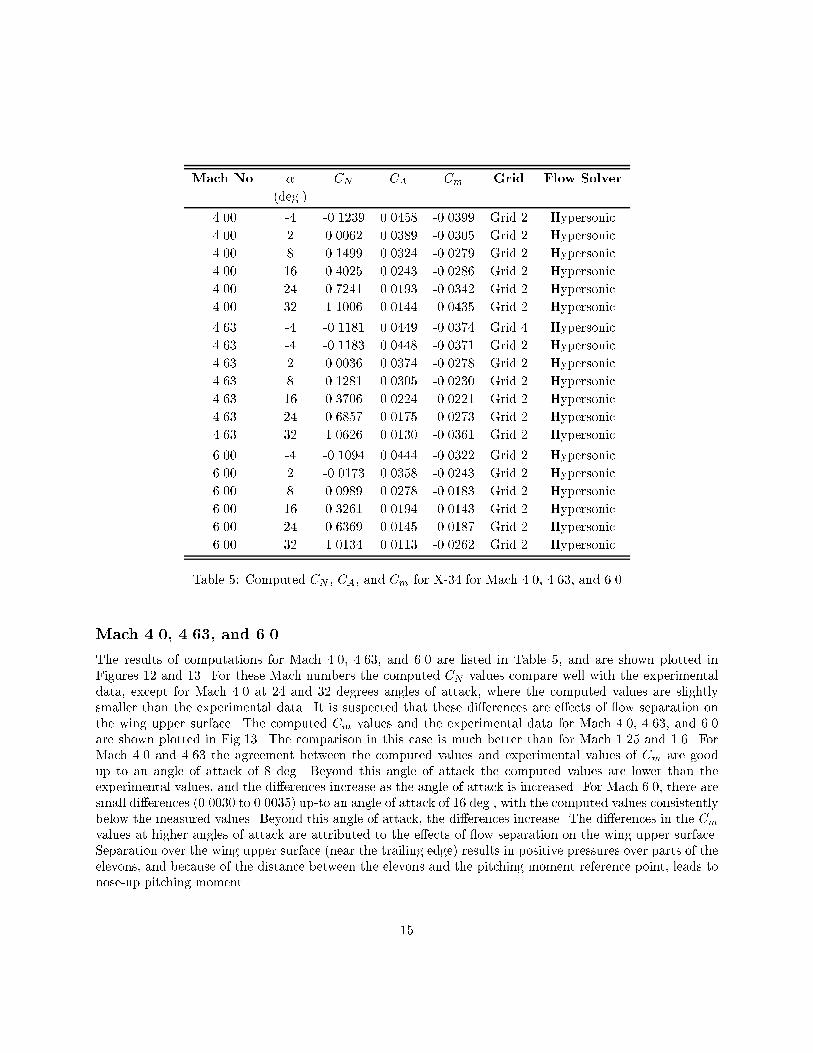
Table 5: Computed CN , CA, and Cm for X-34 for Mach 4.0, 4.63, and 6.0

Mach 4.0, 4.63, and 6.0

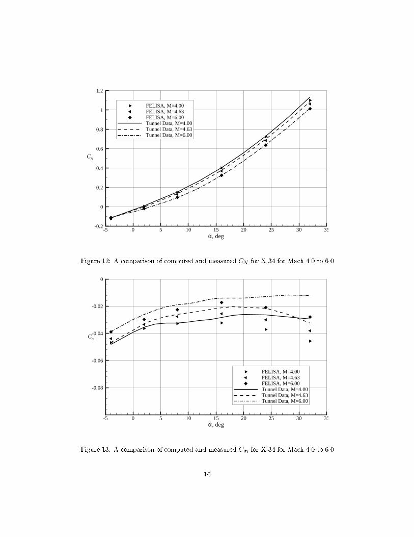
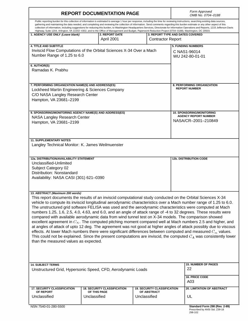
The results of computations for Mach 4.0, 4.63, and 6.0 are listed in Table 5, and are shown plotted inFigures 12 and 13. For these Mach numbers the computed CN values compare well with the experimentaldata, except for Mach 4.0 at 24 and 32 degrees angles of attack, where the computed values are slightlysmaller than the experimental data. It is suspected that these di�erences are e�ects of ow separation onthe wing upper surface. The computed Cm values and the experimental data for Mach 4.0, 4.63, and 6.0are shown plotted in Fig.13. The comparison in this case is much better than for Mach 1.25 and 1.6. ForMach 4.0 and 4.63 the agreement between the computed values and experimental values of Cm are goodup to an angle of attack of 8 deg. Beyond this angle of attack the computed values are lower than theexperimental values, and the di�erences increase as the angle of attack is increased. For Mach 6.0, there aresmall di�erences (0.0030 to 0.0035) up-to an angle of attack of 16 deg., with the computed values consistentlybelow the measured values. Beyond this angle of attack, the di�erences increase. The di�erences in the Cmvalues at higher angles of attack are attributed to the e�ects of ow separation on the wing upper surface.Separation over the wing upper surface (near the trailing edge) results in positive pressures over parts of theelevons, and because of the distance between the elevons and the pitching moment reference point, leads tonose-up pitching moment.

15

-5 0 5 10 15 20 25 30 35α, deg

-0.2

0

0.2

0.4

0.6

0.8

1

1.2

FELISA, M=4.00FELISA, M=4.63FELISA, M=6.00Tunnel Data, M=4.00Tunnel Data, M=4.63Tunnel Data, M=6.00

CN

Figure 12: A comparison of computed and measured CN for X-34 for Mach 4.0 to 6.0

-5 0 5 10 15 20 25 30 35α, deg

-0.08

-0.06

-0.04

-0.02

0

FELISA, M=4.00FELISA, M=4.63FELISA, M=6.00Tunnel Data, M=4.00Tunnel Data, M=4.63Tunnel Data, M=6.00

Cm

Figure 13: A comparison of computed and measured Cm for X-34 for Mach 4.0 to 6.0

16

Conclusions

The results of a computational study conducted on the Orbital Sciences X-34 vehicle to compute the inviscidlongitudinal aerodynamic characteristics are presented. The computational results for a Mach number rangeof 1.25 to 6.0 are compared with available aerodynamic data from wind tunnel tests on the X-34 scale models.The comparison showed that inviscid FELISA software yields normal force coe�cients that compare well withwind tunnel data over the entire Mach number and angle of attack ranges (-4{32 degrees). The computedpitching moment coe�cients compared well at Mach numbers 2.5 and above, at angles of attack of up to12 deg.; beyond this angle of attack, the agreement was not good. At these Mach numbers, the di�erencesbetween the present (inviscid) computational results and the wind tunnel data are attributed to a largeextent to the viscous e�ects which lead to ow separation, particularly over the wing upper surface at largeangles of attack. At lower Mach numbers (1.25 and 1.6) there were signi�cant di�erences between computedand measured pitching moment coe�cient values. These di�erences are also attributed to viscous e�ects.At these Mach numbers, the absence of boundary layer on the wing upper surface leads to di�erences in theshock locations which in turn result in di�erences in the computed and measured aerodynamic data.

Acknowledgments

The author wishes to express his gratitude to Mr. K. J. Weilmuenster and Dr. K. Sutton of the Aerothermo-dynamics Branch (AB), NASA Langley Research Center for many helpful discussions during the course ofthis work. The author also wishes to thank Mr. G. J. Brauckmann of the AB for providing the experimentaldata used in this paper for comparison. The work described herein was performed at Lockheed MartinEngineering & Sciences Company in Hampton, Virginia, and was supported by the AerothermodynamicsBranch, NASA Langley under the contract NAS1-96014. The technical monitor was Mr. Weilmuenster.

References

[1] Freeman, Jr., D.C., Talay, T.A., and Austin, R.E., \Single-Stage-to-Orbit|Meeting the Challenge,"Acta Astronautica, Vol. 38, Nos.4{8, pp. 323-331, 1996.

[2] Peiro, J., Peraire, J., and Morgan, K., \FELISA System Reference Manual and User's Guide," Tech.Report, University College of Swansea, Swansea, U.K., 1993.

[3] Frink, N.T., Pirzadeh, S., and Parikh, P., \An Unstructured-Grid Software System for Solving ComplexAerodynamic Problems," NASA CP-3291, pp. 289-308, May 9-11, 1995.

[4] Samereh, J., \GridTool: A Surface Modeling and Grid Generation Tool," NASA CP 3291, May 1995.

17

REPORT DOCUMENTATION PAGE Form ApprovedOMB No. 0704–0188

Public reporting burden for this collection of information is estimated to average 1 hour per response, including the time for reviewing instructions, searching existing data sources,gathering and maintaining the data needed, and completing and reviewing the collection of information. Send comments regarding this burden estimate or any other aspect of thiscollection of information, including suggestions for reducing this burden, to Washington Headquarters Services, Directorate for Information Operations and Reports, 1215 Jefferson DavisHighway, Suite 1204, Arlington, VA 22202–4302, and to the Office of Management and Budget, Paperwork Reduction Project (0704–0188), Washington, DC 20503.

NSN 7540-01-280-5500 Standard Form 298 (Rev. 2-89)Prescribed by ANSI Std. Z39-18298-102

1. AGENCY USE ONLY (Leave blank) 2. REPORT DATE

April 20013. REPORT TYPE AND DATES COVERED

Contractor Report

4. TITLE AND SUBTITLE

Inviscid Flow Computations of the Orbital Sciences X-34 Over a MachNumber Range of 1.25 to 6.0

5. FUNDING NUMBERS

C NAS1-96014WU 242-80-01-01

6. AUTHOR(S)

Ramadas K. Prabhu

7. PERFORMING ORGANIZATION NAME(S) AND ADDRESS(ES)

Lockheed Martin Engineering & Sciences CompanyC/O NASA Langley Research CenterHampton, VA 23681–2199

8. PERFORMING ORGANIZATIONREPORT NUMBER

9. SPONSORING/MONITORING AGENCY NAME(S) AND ADDRESS(ES)

NASA Langley Research CenterHampton, VA 23681–2199

10. SPONSORING/MONITORINGAGENCY REPORT NUMBER

NASA/CR–2001–210849

11. SUPPLEMENTARY NOTES

Langley Technical Monitor: K. James Weilmuenster

12a. DISTRIBUTION/AVAILABILITY STATEMENT

Unclassified-UnlimitedSubject Category 02Distribution: NonstandardAvailability: NASA CASI (301) 621–0390

12b. DISTRIBUTION CODE

13. ABSTRACT (Maximum 200 words)

This report documents the results of an inviscid computational study conducted on the Orbital Sciences X-34vehicle to compute its inviscid longitudinal aerodynamic characteristics over a Mach number range of 1.25 to 6.0.The unstructured grid software FELISA was used and the aerodynamic characteristics were computed at Machnumbers 1.25, 1.6, 2.5, 4.0, 4.63, and 6.0, and an angle of attack range of -4 to 32 degrees. These results werecompared with available aerodynamic data from wind tunnel test on X-34 models. The comparison showedexcellent agreement in CN . The computed pitching moment compared well at Mach numbers 2.5 and higher, andat angles of attack of upto 12 deg. The agreement was not good at higher angles of attack possibly due to viscouseffects. At lower Mach numbers there were significant differences between computed and measured Cm values.This could not be explained. Since the present computations are inviscid, the computed CA was consistently lowerthan the measured values as expected.

14. SUBJECT TERMS

Unstructured Grid, Hypersonic Speed, CFD, Aerodynamic Loads15. NUMBER OF PAGES

22

16. PRICE CODE

A03

17. SECURITY CLASSIFICATIONOF REPORT

Unclassified

18. SECURITY CLASSIFICATIONOF THIS PAGE

Unclassified

19. SECURITY CLASSIFICATIONOF ABSTRACT

Unclassified

20. LIMITATION OF ABSTRACT

UL