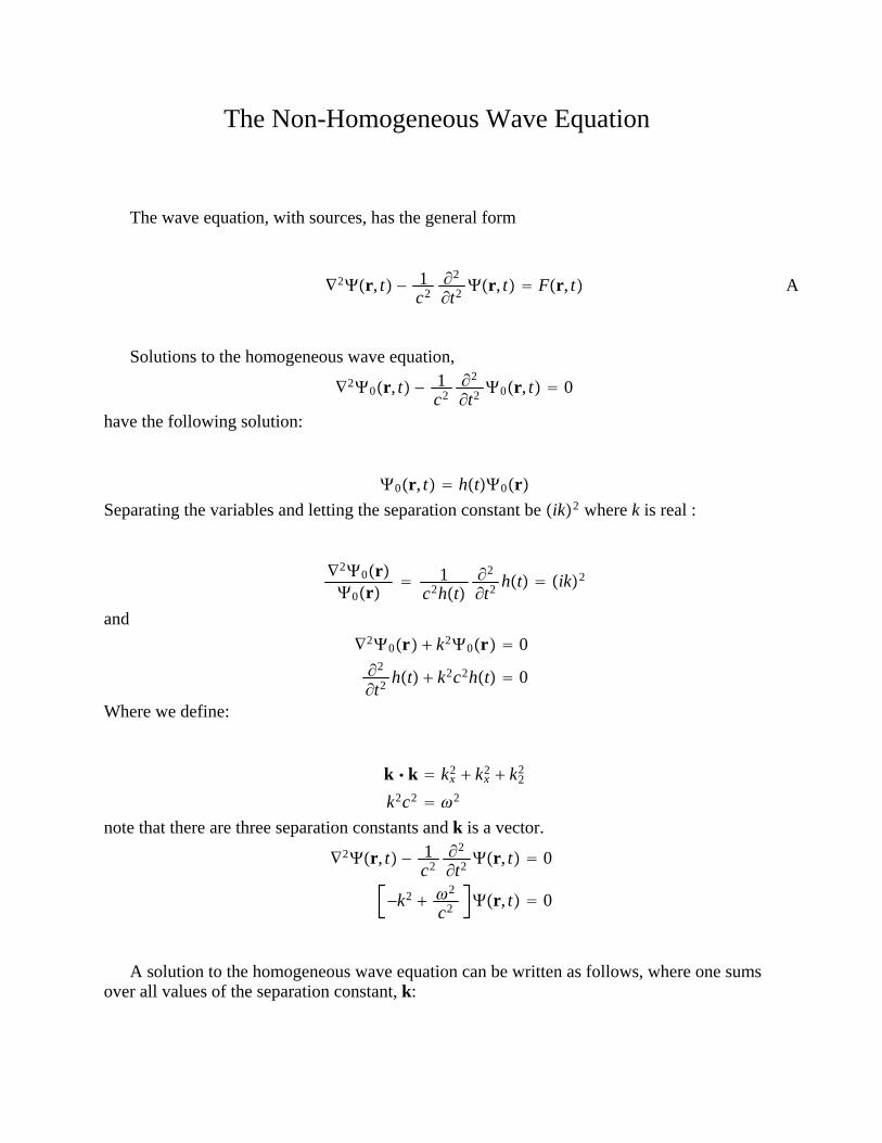
The Non-Homogeneous Wave Equation

The wave equation, with sources, has the general form

∇2r, t − 1c2∂2

∂t2 r, t Fr, t A

Solutions to the homogeneous wave equation,

∇20r, t − 1c2∂2

∂t2 0r, t 0

have the following solution:

0r, t ht0r

Separating the variables and letting the separation constant be ik2 where k is real :

∇20r0r

1c2ht

∂2

∂t2 ht ik2

and

∇20r k20r 0

∂2

∂t2 ht k2c2ht 0

Where we define:

k k kx2 kx

2 k22

k2c2 2

note that there are three separation constants and k is a vector.

∇2r, t − 1c2∂2

∂t2 r, t 0

−k2 2

c2 r, t 0

A solution to the homogeneous wave equation can be written as follows, where one sumsover all values of the separation constant, k:

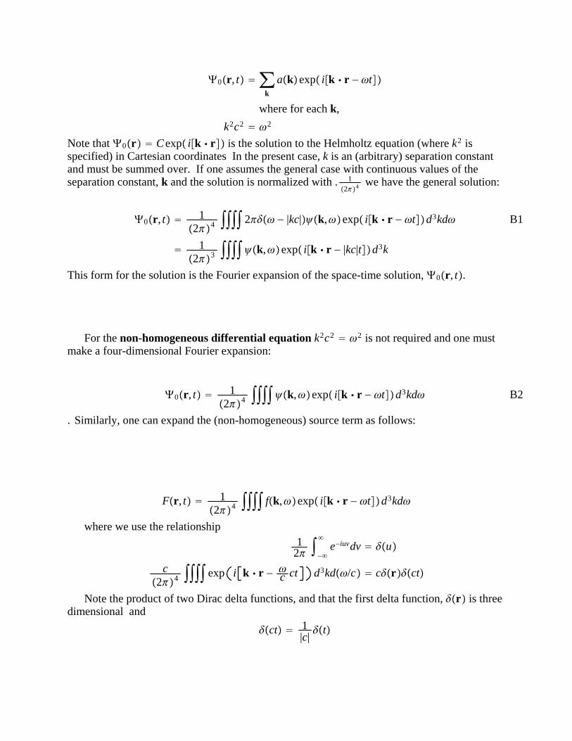
0r, t ∑k

akexp ik r − t

where for each k,

k2c2 2

Note that 0r Cexp ik r is the solution to the Helmholtz equation (where k2 isspecified) in Cartesian coordinates In the present case, k is an (arbitrary) separation constantand must be summed over. If one assumes the general case with continuous values of theseparation constant, k and the solution is normalized with . 1

24 we have the general solution:

0r, t 124 2 − |kc|k,exp ik r − td3kd

123 k,exp ik r − |kc|td3k

B1

This form for the solution is the Fourier expansion of the space-time solution, 0r, t.

For the non-homogeneous differential equation k2c2 2 is not required and one mustmake a four-dimensional Fourier expansion:

0r, t 124 k,exp ik r − td3kd B2

. Similarly, one can expand the (non-homogeneous) source term as follows:

Fr, t 124 fk,exp ik r − td3kd

where we use the relationship1

2 −

e−iuvdv u

c24 exp i k r −

c ct d3kd/c crct

Note the product of two Dirac delta functions, and that the first delta function, r is threedimensional and

ct 1|c|t

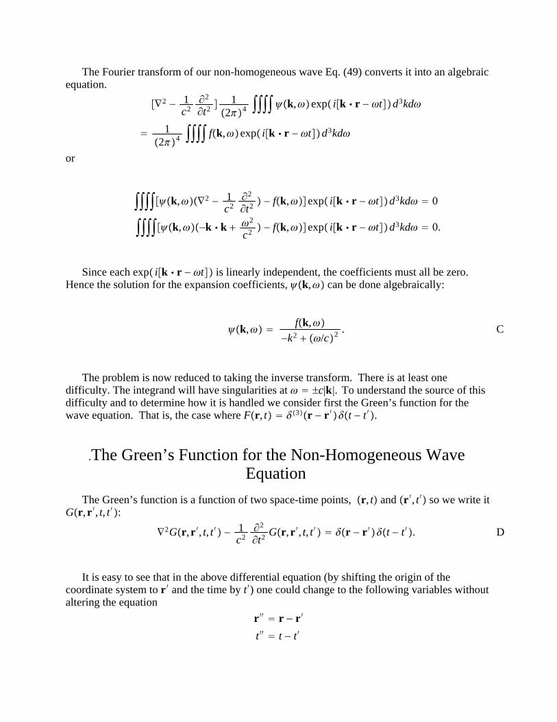
The Fourier transform of our non-homogeneous wave Eq. (49) converts it into an algebraicequation.

∇2 − 1c2∂2

∂t2 1

24 k,exp ik r − td3kd

124 fk,exp ik r − td3kd

or

k,∇2 − 1c2∂2

∂t2 − fk,exp ik r − td3kd 0

k,−k k 2

c2 − fk,exp ik r − td3kd 0.

Since each exp ik r − t is linearly independent, the coefficients must all be zero.Hence the solution for the expansion coefficients, k, can be done algebraically:

k, fk,

−k2 /c2 . C

The problem is now reduced to taking the inverse transform. There is at least onedifficulty. The integrand will have singularities at c|k|. To understand the source of thisdifficulty and to determine how it is handled we consider first the Green’s function for thewave equation. That is, the case where Fr, t 3r − r ′t − t ′.

.The Green’s Function for the Non-Homogeneous WaveEquation

The Green’s function is a function of two space-time points, r, t and r ′, t ′ so we write itGr,r ′, t, t ′:

∇2Gr,r ′, t, t ′ − 1c2∂2

∂t2 Gr,r ′, t, t ′ r − r ′t − t ′. D

It is easy to see that in the above differential equation (by shifting the origin of thecoordinate system to r ′ and the time by t ′) one could change to the following variables withoutaltering the equation

r ′′ r − r ′

t ′′ t − t ′

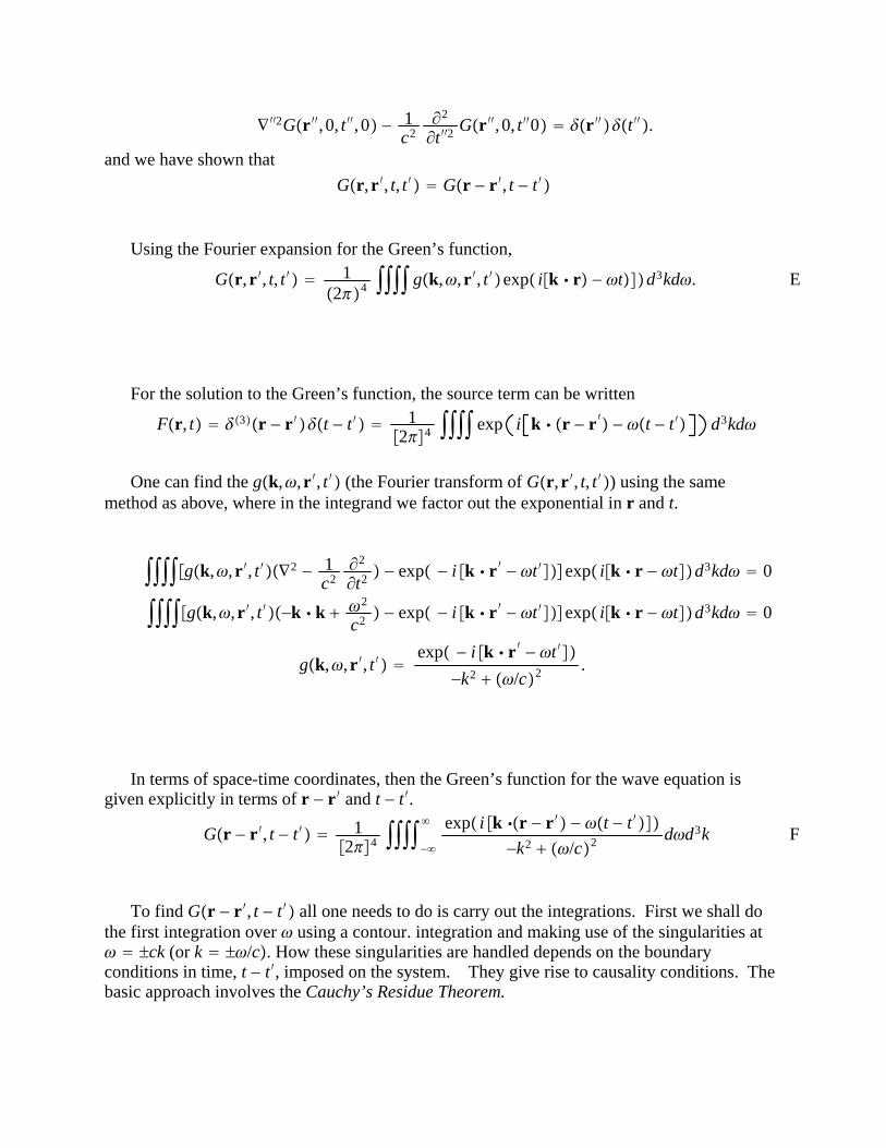
∇′′2Gr ′′, 0, t ′′, 0 − 1c2∂2

∂t ′′2Gr ′′, 0, t ′′0 r ′′t ′′.

and we have shown that

Gr,r ′, t, t ′ Gr − r ′, t − t ′

Using the Fourier expansion for the Green’s function,

Gr,r ′, t, t ′ 124 gk,,r ′, t ′exp ik r − td3kd. E

For the solution to the Green’s function, the source term can be written

Fr, t 3r − r ′t − t ′ 124 exp i k r − r ′ − t − t ′ d3kd

One can find the gk,,r ′, t ′ (the Fourier transform of Gr,r ′, t, t ′) using the samemethod as above, where in the integrand we factor out the exponential in r and t.

gk,,r ′, t ′∇2 − 1c2∂2

∂t2 − exp − i k r ′ − t ′ exp ik r − td3kd 0

gk,,r ′, t ′−k k 2

c2 − exp − i k r ′ − t ′ exp ik r − td3kd 0

gk,,r ′, t ′ exp − i k r ′ − t ′

−k2 /c2 .

In terms of space-time coordinates, then the Green’s function for the wave equation isgiven explicitly in terms of r − r ′ and t − t ′.

Gr − r ′, t − t ′ 124 −

exp i k r − r ′ − t − t ′−k2 /c2 dd3k F

To find Gr − r ′, t − t ′ all one needs to do is carry out the integrations. First we shall dothe first integration over using a contour. integration and making use of the singularities at ck (or k /c. How these singularities are handled depends on the boundaryconditions in time, t − t ′, imposed on the system. They give rise to causality conditions. Thebasic approach involves the Cauchy’s Residue Theorem.

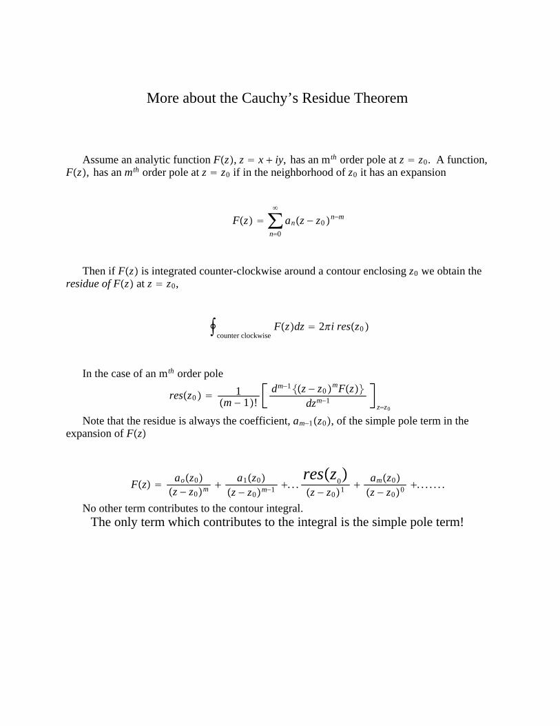
More about the Cauchy’s Residue Theorem

Assume an analytic function Fz, z x iy, has an mth order pole at z z0. A function,Fz, has an mth order pole at z z0 if in the neighborhood of z0 it has an expansion

Fz ∑n0

anz − z0n−m

Then if Fz is integrated counter-clockwise around a contour enclosing z0 we obtain theresidue of Fz at z z0,

counter clockwise

Fzdz 2i resz0

In the case of an mth order pole

resz0 1m − 1!

dm−1z − z0mFzdzm−1

zz0

Note that the residue is always the coefficient, am−1z0, of the simple pole term in theexpansion of Fz

Fz aoz0z − z0m a1z0

z − z0m−1 . . .resz

0

z − z01 amz0z − z00 . . . . . . .

No other term contributes to the contour integral.The only term which contributes to the integral is the simple pole term!

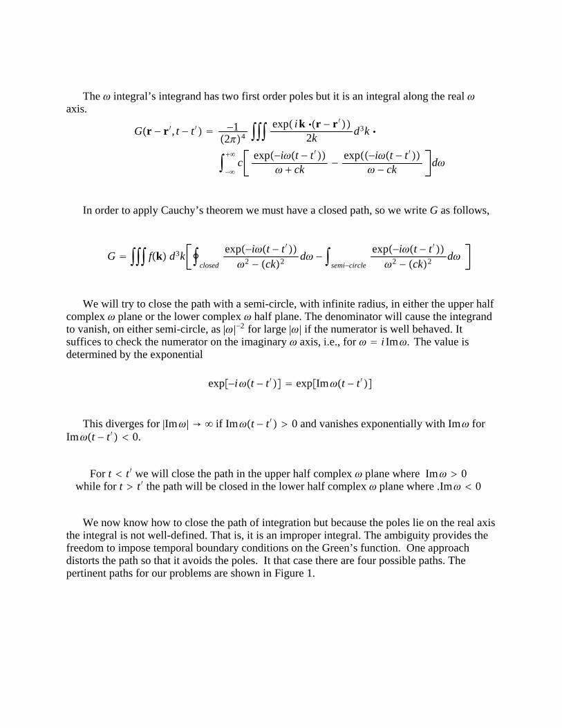
The integral’s integrand has two first order poles but it is an integral along the real axis.

Gr − r ′, t − t ′ −124

exp ik r − r ′2k

d3k

−

c

exp−it − t ′ ck

−exp−it − t ′

− ckd

In order to apply Cauchy’s theorem we must have a closed path, so we write G as follows,

G fk d3k closed

exp−it − t ′2 − ck2 d −

semi−circle

exp−it − t ′2 − ck2 d

We will try to close the path with a semi-circle, with infinite radius, in either the upper halfcomplex plane or the lower complex half plane. The denominator will cause the integrandto vanish, on either semi-circle, as ||−2 for large || if the numerator is well behaved. Itsuffices to check the numerator on the imaginary axis, i.e., for i Im. The value isdetermined by the exponential

exp−it − t ′ expImt − t ′

This diverges for |Im| → if Imt − t ′ 0 and vanishes exponentially with Im forImt − t ′ 0.

For t t ′ we will close the path in the upper half complex plane where Im 0while for t t ′ the path will be closed in the lower half complex plane where .Im 0

We now know how to close the path of integration but because the poles lie on the real axisthe integral is not well-defined. That is, it is an improper integral. The ambiguity provides thefreedom to impose temporal boundary conditions on the Green’s function. One approachdistorts the path so that it avoids the poles. It that case there are four possible paths. Thepertinent paths for our problems are shown in Figure 1.

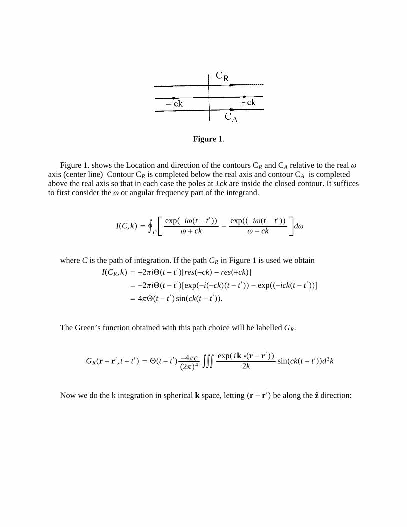
Figure 1.

Figure 1. shows the Location and direction of the contours CR and CA relative to the real axis (center line) Contour CR is completed below the real axis and contour CA is completedabove the real axis so that in each case the poles at ck are inside the closed contour. It sufficesto first consider the or angular frequency part of the integrand.

IC,k C

exp−it − t ′ ck

−exp−it − t ′

− ckd

where C is the path of integration. If the path CR in Figure 1 is used we obtain

ICR,k −2iΘt − t ′res−ck − resck

−2iΘt − t ′exp−i−ckt − t ′ − exp−ickt − t ′

4Θt − t ′ sinckt − t ′.

The Green’s function obtained with this path choice will be labelled GR.

GRr − r ′, t − t ′ Θt − t ′ −4c24

exp ik r − r ′2k

sinckt − t ′d3k

Now we do the k integration in spherical k space, letting r − r ′ be along the z direction:

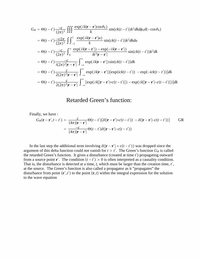
GR Θt − t ′ −c23

exp i k|r − r ′|coskk

sinckt − t ′k2dkdkd−cosk

Θt − t ′ −c223 −1

1 exp i k|r − r ′|uk

sinckt − t ′k2dkdu

Θt − t ′ −c22 0

exp i k|r − r ′| − exp− i k|r − r ′|ik2|r − r ′|

sinckt − t ′k2dk

Θt − t ′ −ci22|r − r ′|

−

exp i k|r − r ′| sinckt − t ′dk

Θt − t ′ c222|r − r ′|

−

exp i k|r − r ′|expickt − t ′ − exp−ickt − t ′dk

Θt − t ′ c222|r − r ′|

−

exp i k|r − r ′|ct − t ′ − exp i k|r − r ′|−ct − t ′dk

Retarded Green’s function:

Finally, we have :

GRr − r ′, t − t ′ c4|r − r ′|

Θt − t ′|r − r ′|ct − t ′ − |r − r ′|−ct − t ′

−c4|r − r ′|

Θt − t ′|r − r ′|−ct − t ′

GR

In the last step the additional term involving |r − r ′ | ct − t ′ was dropped since theargument of this delta function could not vanish for t t ′. The Green’s function GR is calledthe retarded Green’s function. It gives a disturbance (created at time t ′) propagating outwardfrom a source point r ′. The condition t − t ′ 0 is often interpreted as a causality condition.That is, the disturbance is detected at a time, t, which must be larger than the creation time, t ′,at the source. The Green’s function is also called a propagator as it ”propagates” thedisturbance from point r ′, t ′ to the point r, t within the integral expression for the solutionto the wave equation

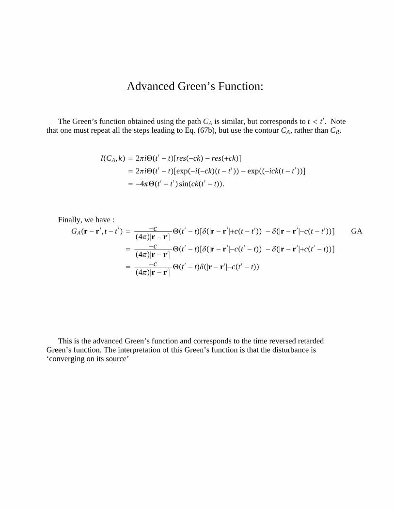
Advanced Green’s Function:

The Green’s function obtained using the path CA is similar, but corresponds to t t ′. Notethat one must repeat all the steps leading to Eq. (67b), but use the contour CA, rather than CR.

ICA,k 2iΘt ′ − tres−ck − resck

2iΘt ′ − texp−i−ckt − t ′ − exp−ickt − t ′

−4Θt ′ − t ′ sinckt ′ − t.

Finally, we have :

GAr − r ′, t − t ′ −c4|r − r ′|

Θt ′ − t|r − r ′|ct − t ′ − |r − r ′|−ct − t ′

−c4|r − r ′|

Θt ′ − t|r − r ′|−ct ′ − t − |r − r ′|ct ′ − t

−c4|r − r ′|

Θt ′ − t|r − r ′|−ct ′ − t

GA

This is the advanced Green’s function and corresponds to the time reversed retardedGreen’s function. The interpretation of this Green’s function is that the disturbance is‘converging on its source’

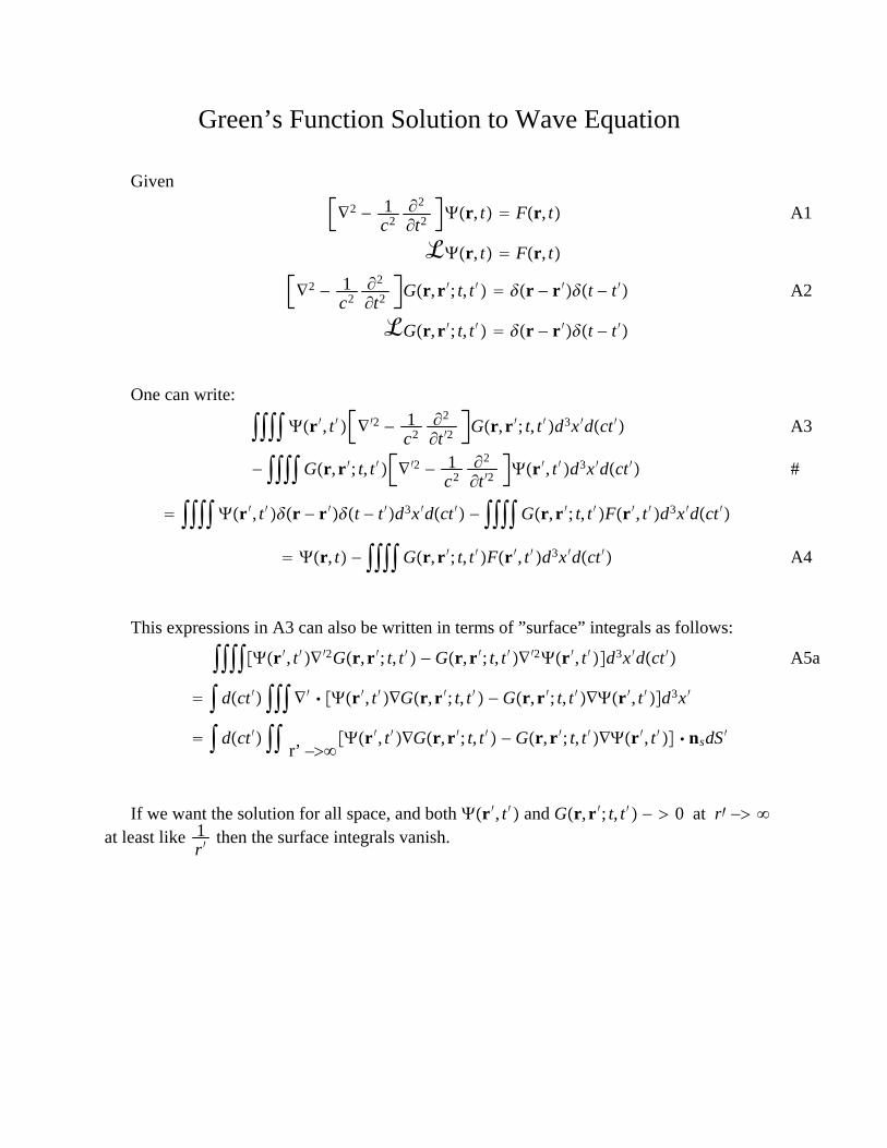
Green’s Function Solution to Wave Equation

Given

∇2 − 1c2∂2

∂t2 r, t Fr, t

ℒr, t Fr, t

A1

∇2 − 1c2∂2

∂t2 Gr,r ′; t, t ′ r − r ′t − t ′

ℒGr,r ′; t, t ′ r − r ′t − t ′

A2

One can write:

r ′, t ′ ∇′2 − 1c2∂2

∂t ′2Gr,r ′; t, t ′d3x ′dct ′

− Gr,r ′; t, t ′ ∇′2 − 1c2∂2

∂t ′2r ′, t ′d3x ′dct ′

A3

#

r ′, t ′r − r ′t − t ′d3x ′dct ′ − Gr,r ′; t, t ′Fr ′, t ′d3x ′dct ′

r, t − Gr,r ′; t, t ′Fr ′, t ′d3x ′dct ′ A4

This expressions in A3 can also be written in terms of ”surface” integrals as follows:

r ′, t ′∇′2Gr,r ′; t, t ′ − Gr,r ′; t, t ′∇′2r ′, t ′d3x ′dct ′

dct ′ ∇′ r ′, t ′∇Gr,r ′; t, t ′ − Gr,r ′; t, t ′∇r ′, t ′d3x ′

dct ′ r’ –

r ′, t ′∇Gr,r ′; t, t ′ − Gr,r ′; t, t ′∇r ′, t ′ nsdS′

A5a

If we want the solution for all space, and both r ′, t ′ and Gr,r ′; t, t ′ − 0 at r′ − at least like 1

r′then the surface integrals vanish.

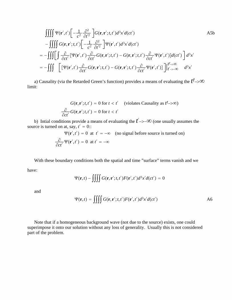
r ′, t ′ − 1c2∂2

∂t ′2Gr,r ′; t, t ′d3x ′dct ′

− Gr,r ′; t, t ′ − 1c2∂2

∂t ′2r ′, t ′d3x ′dct ′

− ∂∂ct ′

r ′, t ′ ∂∂ct ′

Gr,r ′; t, t ′ − Gr,r ′; t, t ′ ∂∂ct ′

r ′, t ′dct ′ d3x ′

− r ′, t ′ ∂∂ct ′

Gr,r ′; t, t ′ − Gr,r ′; t, t ′ ∂∂ct ′

r ′, t ′ |t′–−t′–

d3x ′

A5b

a) Causality (via the Retarded Green’s function) provides a means of evaluating the t′–limit:

Gr,r ′; t, t ′ 0 for t t ′ (violates Causality as t′–)

∂∂ct ′

Gr,r ′; t, t ′ 0 for t t ′

b) Intial conditions provide a means of evaluating the t′–− (one usually assumes thesource is turned on at, say, t ′ 0::

r ′, t ′ 0 at t ′ − (no signal before source is turned on)

∂∂ct ′

r ′, t ′ 0 at t ′ −

With these boundary conditions both the spatial and time ”surface” terms vanish and we

have:

r, t − Gr,r ′; t, t ′Fr ′, t ′d3x ′dct ′ 0

and

r, t Gr,r ′; t, t ′Fr ′, t ′d3x ′dct ′ A6

Note that if a homogeneous background wave (not due to the source) exists, one couldsuperimpose it onto our solution without any loss of generality. Usually this is not consideredpart of the problem.

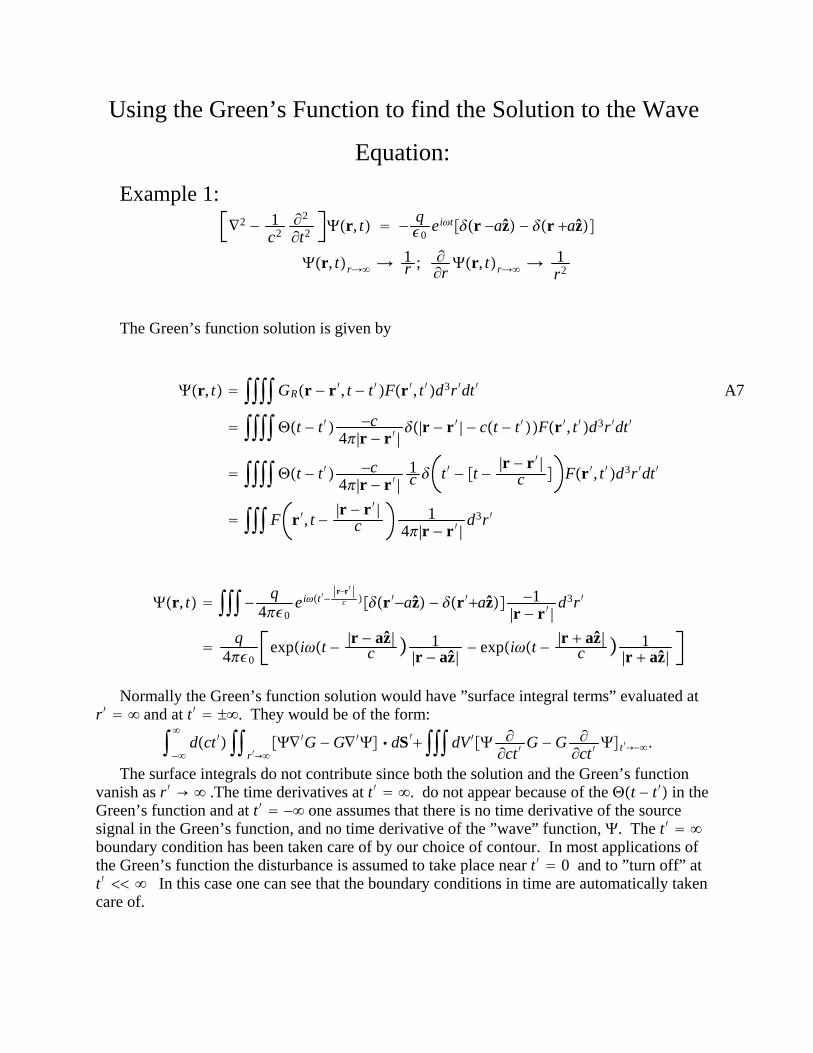
Using the Green’s Function to find the Solution to the Wave

Equation:

Example 1:

∇2 − 1c2∂2

∂t2 r, t − q0

eitr −az − r az

r, tr 1r ; ∂∂rr, tr

1r2

The Green’s function solution is given by

r, t GRr − r ′, t − t ′Fr ′, t ′d3r′dt ′

Θt − t ′ −c4|r − r ′ |

|r − r ′ | − ct − t ′Fr ′, t ′d3r′dt ′

Θt − t ′ −c4|r − r ′ |

1c t ′ − t − |r − r ′ |

c Fr ′, t ′d3r′dt ′

F r ′, t − |r − r ′ |c

14|r − r ′ |

d3r′

A7

r, t − q40

eit′−r−r′

c r ′−az − r ′az −1|r − r ′ |

d3r′

q40

expit − |r − az|c 1

|r − az|− expit − |r az|

c 1|r az|

Normally the Green’s function solution would have ”surface integral terms” evaluated atr′ and at t ′ . They would be of the form:

−

dct ′

r′→∇′G − G∇′ dS′ dV ′ ∂

∂ct ′G − G ∂

∂ct ′t′→−.

The surface integrals do not contribute since both the solution and the Green’s functionvanish as r′ → .The time derivatives at t ′ . do not appear because of the Θt − t ′ in theGreen’s function and at t ′ − one assumes that there is no time derivative of the sourcesignal in the Green’s function, and no time derivative of the ”wave” function, . The t ′ boundary condition has been taken care of by our choice of contour. In most applications ofthe Green’s function the disturbance is assumed to take place near t ′ 0 and to ”turn off” att ′ In this case one can see that the boundary conditions in time are automatically takencare of.

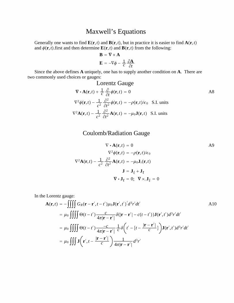
Maxwell’s Equations

Generally one wants to find Er, t and Br, t, but in practice it is easier to find Ar, tand r, t.first and then determine Er, t and Br, t from the following:

B ∇ A

E −∇ − 1c∂A∂t

Since the above defines A uniquely, one has to supply another condition on A. There aretwo commonly used choices or gauges:

Lorentz Gauge∇ Ar, t 1

c∂∂tr, t 0

∇2r, t − 1c2∂2

∂t2 r, t −r, t/0 S.I. units

∇2Ar, t − 1c2∂2

∂t2 Ar, t −0Jr, t S.I. units

A8

Coulomb/Radiation Gauge

∇ Ar, t 0

∇2r, t −r, t/0

∇2Ar, t − 1c2∂2

∂t2 Ar, t −0Jtr, t

J Jℓ Jt

∇ Jt 0; ∇ .Jℓ 0

A9

In the Lorentz gauge:

Ar, t −GRr − r ′, t − t ′0Jr ′, t ′′d3r′dt ′

0 Θt − t ′ c4|r − r ′ |

|r − r ′ | − ct − t ′Jr ′, t ′d3r′dt ′

0 Θt − t ′ −c4|r − r ′ |

1c t ′ − t − |r − r ′ |

c Jr ′, t ′d3r′dt ′

0 J r ′, t − |r − r ′ |c

14|r − r ′ |

d3r′

A10

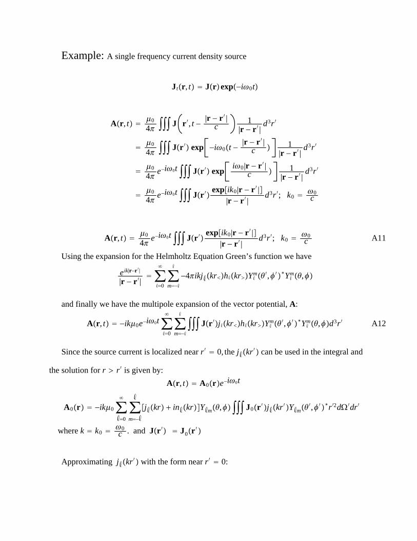
Example: A single frequency current density source

Jtr, t Jrexp−i0t

Ar, t 0

4 J r ′, t − |r − r ′ |c

1|r − r ′ |

d3r′

0

4 Jr ′ exp −i0t −|r − r ′ |

c 1|r − r ′ |

d3r′

0

4e−i0t Jr ′ exp

i0|r − r ′ |c 1

|r − r ′ |d3r′

0

4e−i0t Jr ′

expik0|r − r ′ ||r − r ′ |

d3r′; k0 0c

Ar, t 0

4e−i0t Jr ′

expik0|r − r ′ ||r − r ′ |

d3r′; k0 0c A11

Using the expansion for the Helmholtz Equation Green’s function we have

eik|r−r′|

|r − r ′|∑

ℓ0

∑m−ℓ

ℓ

−4ikjℓkrhℓkrYℓm ′, ′∗Yℓ

m,

and finally we have the multipole expansion of the vector potential, A:

Ar, t −ik0e−i0t∑ℓ0

∑m−ℓ

ℓ

Jr ′jℓkrhℓkrYℓm ′, ′∗Yℓ

m,d3r′ A12

Since the source current is localized near r′ 0, the jℓkr′ can be used in the integral and

the solution for r r′ is given by:

Ar, t A0re−i0t

A0r −ik0∑ℓ0

∑m−ℓ

ℓjℓkr inℓkrYℓm, J0r ′jℓkr′Yℓm

′, ′∗r′2d′dr′

where k k0 0c . and Jr ′ J0r

′

Approximating jℓkr′ with the form near r′ 0:

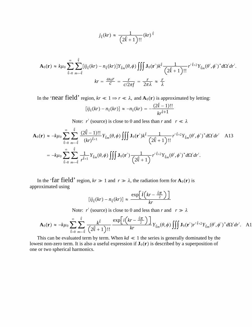
jℓkr ≈ 12ℓ 1 !!

kr ℓ

A0r ≈ k0∑ℓ0

∑m−ℓ

ℓijℓkr − nℓkrYℓm, J0r ′kℓ 1

2ℓ 1 !!r′ ℓ2Yℓm

′, ′∗d′dr′.

kr 0rc r

c/2f r

2≈ r

In the ‘near field’ region, kr 1 r , and A0r is approximated by letting:

ijℓkr − nℓkr ≈ −nℓkr − 2ℓ − 1!!

krℓ1

Note: r′ (source) is close to 0 and less than r and r

A0r ≈ −k0∑ℓ0

∑m−ℓ

ℓ2ℓ − 1!!

krℓ1Yℓm, J0r ′kℓ 1

2ℓ 1 !!r′ ℓ2Yℓm

′, ′∗d′dr′

−k0∑ℓ0

∑m−ℓ

ℓ1

rℓ1Yℓm, J0r ′ 1

2ℓ 1r′ ℓ2Yℓm

′, ′∗d′dr′.

A13

In the ‘far field’ region, kr 1 and r , the radiation form for A0r isapproximated using

ijℓkr − nℓkr ≈exp i kr − ℓ

2

kr

Note: r′ (source) is close to 0 and less than r and r

A0r ≈ −k0∑ℓ0

∑m−ℓ

ℓkℓ

2ℓ 1 !!

exp i kr − ℓ2

krYℓm, J0r ′r′ ℓ2Yℓm

′, ′∗d′dr′. A14

This can be evaluated term by term. When kd 1 the series is generally dominated by thelowest non-zero term. It is also a useful expression if J0r is described by a superposition ofone or two spherical harmonics.

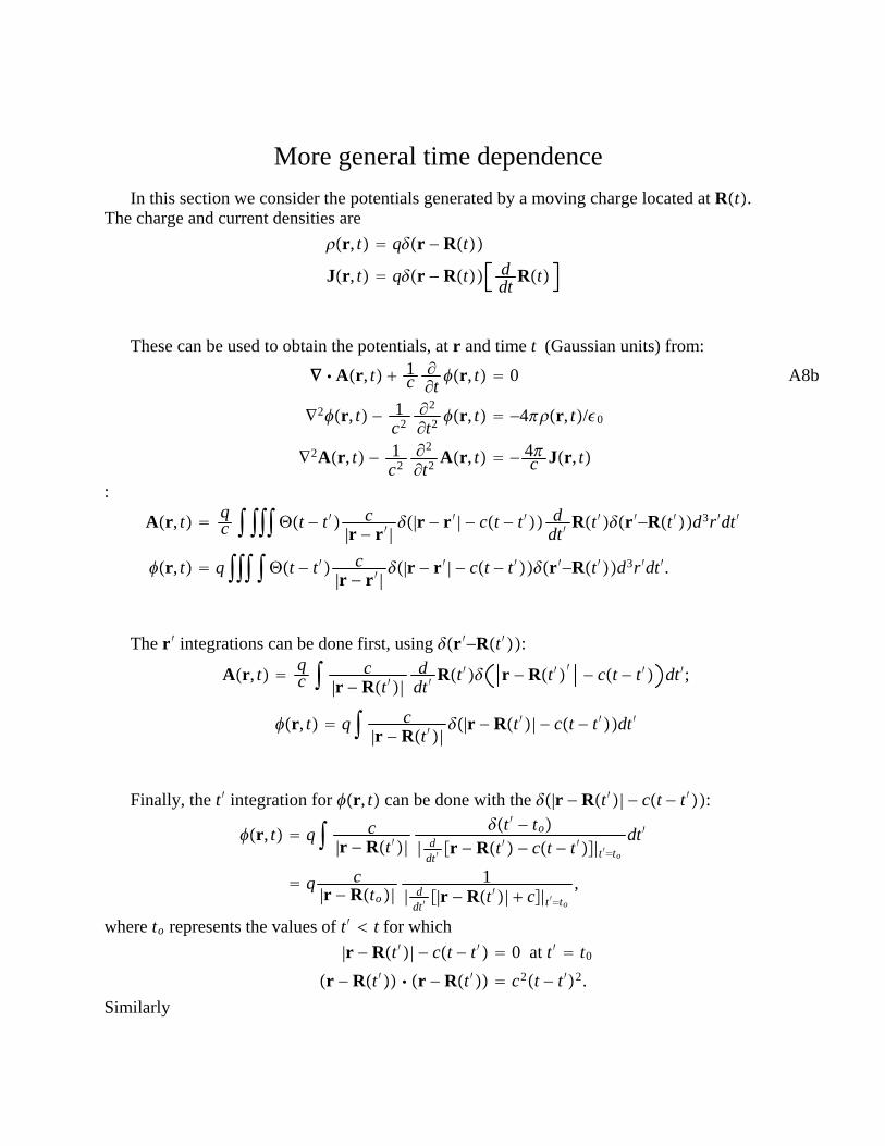
More general time dependence

In this section we consider the potentials generated by a moving charge located at Rt.The charge and current densities are

r, t qr − Rt

Jr, t qr − Rt ddt

Rt

These can be used to obtain the potentials, at r and time t (Gaussian units) from:

∇ Ar, t 1c∂∂tr, t 0

∇2r, t − 1c2∂2

∂t2 r, t −4r, t/0

∇2Ar, t − 1c2∂2

∂t2 Ar, t − 4c Jr, t

A8b

:

Ar, t qc Θt − t ′ c

|r − r ′ ||r − r ′ | − ct − t ′ d

dt ′Rt ′r ′−Rt ′d3r′dt ′

r, t q Θt − t ′ c|r − r ′ |

|r − r ′ | − ct − t ′r ′−Rt ′d3r′dt ′.

The r ′ integrations can be done first, using r ′−Rt ′:

Ar, t qc c

|r − Rt ′|d

dt ′Rt ′ r − Rt ′ ′ − ct − t ′ dt ′;

r, t q c|r − Rt ′|

|r − Rt ′| − ct − t ′dt ′

Finally, the t ′ integration for r, t can be done with the |r − Rt ′| − ct − t ′:

r, t q c|r − Rt ′|

t ′ − to| d

dt′r − Rt ′ − ct − t ′|t′to

dt ′

q c|r − Rto|

1| d

dt′|r − Rt ′| c|t′to

,

where to represents the values of t ′ t for which

|r − Rt ′| − ct − t ′ 0 at t ′ t0

r − Rt ′ r − Rt ′ c2t − t ′2.

Similarly

Ar, t qc

c|r − Rto|

ddt′

Rt ′|t′to

| ddt′ r − Rt ′ ′ c|t′to

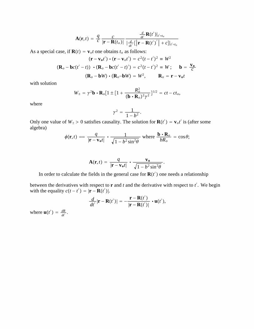
As a special case, if Rt vot one obtains to as follows:

r − vot ′ r − vot ′ c2t − t ′2 ≡ W2

Ro − bct ′ − t Ro − bct ′ − t ′ c2t − t ′2 ≡ W ; b voc

Ro − bW Ro−bW W2, Ro r − vot

with solution

W 2b Ro1 1 Ro

2

b Ro22 1/2 ct − cto,

where

2 11 − b2 .

Only one value of W 0 satisfies causality. The solution for Rt ′ vot ′ is (after somealgebra)

r, t q|r − vot|

11 − b2 sin2

where b Ro

bRo cos;

Ar, t q|r − vot|

vo

1 − b2 sin2.

In order to calculate the fields in the general case for Rt ′ one needs a relationship

between the derivatives with respect to r and t and the derivative with respect to t ′. We beginwith the equality ct − t ′ |r − Rt ′|.

ddt ′

|r − Rt ′| −r − Rt ′|r − Rt ′|

ut ′,

where ut ′ dRdt′

.

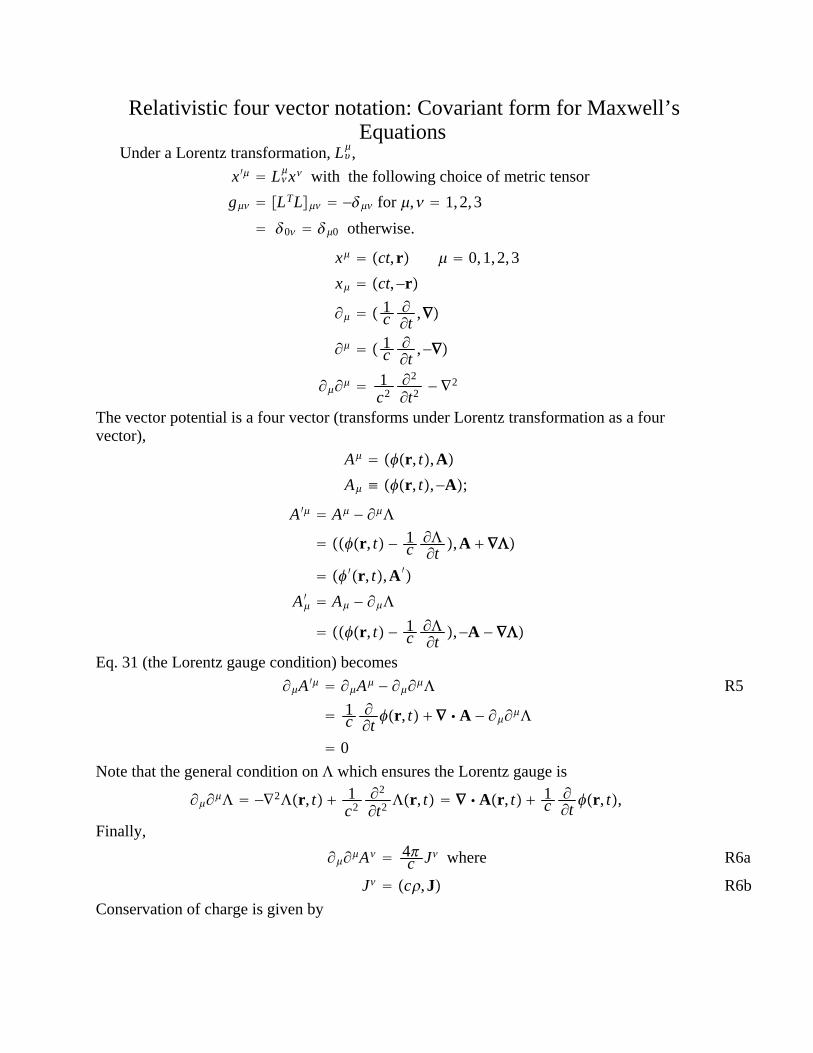
Relativistic four vector notation: Covariant form for Maxwell’sEquations

Under a Lorentz transformation, L,

x ′ Lx with the following choice of metric tensor

g LTL − for , 1,2,3

0 0 otherwise.

x ct,r 0,1,2,3

x ct,−r

∂ 1c∂∂t

,∇

∂ 1c∂∂t

,−∇

∂∂ 1c2∂2

∂t2 − ∇2

The vector potential is a four vector (transforms under Lorentz transformation as a fourvector),

A r, t,A

A ≡ r, t,−A;

A ′ A − ∂

r, t − 1c∂∂t,A ∇

′r, t,A′

A′ A − ∂

r, t − 1c∂∂t,−A − ∇

Eq. 31 (the Lorentz gauge condition) becomes

∂A ′ ∂A − ∂∂

1c∂∂tr, t ∇ A − ∂∂

0

R5

Note that the general condition on which ensures the Lorentz gauge is

∂∂ −∇2r, t 1c2∂2

∂t2 r, t ∇ Ar, t 1c∂∂tr, t,

Finally,

∂∂A 4c J where

J c,J

R6a

R6b

Conservation of charge is given by

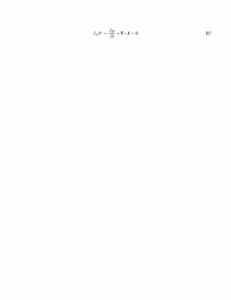
∂J ∂∂t

∇ J 0 R7