the new york state energy research and development authority
TRANSCRIPT

GE Energy
Report for:
The New York State Energy Research and Development Authority Analysis of the Near Term Impact of Proposed Green House Gas Policies on the New York Electric Power System
Project # 10465
Sundar Venkataraman Amanvir Chahal
25 July 2010

1395BThe New York State Energy Research and Development Authority Foreword
GE EA&SE i
FOREWORD
This document was prepared by General Electric International, Inc. acting through its GE Energy Applications and Systems Engineering (EA&SE) business in Schenectady, NY. It is submitted to the New York State Energy Research and Development Authority.
General Electric International, Inc. One River Rd.
Schenectady, NY 12345 USA

1395BThe New York State Energy Research and Development Authority Legal Notices
GE EA&SE ii
LEGAL NOTICES
This report was prepared by General Electric International, Inc. (GEII) acting through its GE Energy Applications and Systems Engineering (EA&SE) business, as an account of work sponsored by the New York State Energy Research and Development Authority (NYSERDA). Neither NYSERDA nor GEII, nor any person acting on behalf of either:
1. Makes any warranty or representation, expressed or implied, with respect to the use of any information contained in this report, or that the use of any information, apparatus, method, or process disclosed in the report may not infringe privately owned rights.
2. Assumes any liabilities with respect to the use of or for damage resulting from the use of any information, apparatus, method, or process disclosed in this report.
Copyright © 2006 GE Energy. All rights reserved

1395BThe New York State Energy Research and Development Authority Table of Contents
GE EA&SE iii
TABLE OF CONTENTS
FOREWORD ................................................................................................................................... I
LEGAL NOTICES.......................................................................................................................... II
TABLE OF CONTENTS .............................................................................................................. III
1 INTRODUCTION ................................................................................................................... 1 1.1 Background ................................................................................................................................... 1 1.2 Need for the Study ........................................................................................................................ 2 1.3 Objectives of the Study ................................................................................................................. 2 1.4 Benefits of the Study ..................................................................................................................... 3
1.4.1 Create public awareness on the impact of GHG policies ...................................................... 3 1.4.2 Provide guidance to Federal and state governments on impacts of GHG policies ............... 3 1.4.3 Provide direction to stakeholders in New York on impacts of GHG policies ...................... 4 1.4.4 Ensure reliability and access to power is not compromised.................................................. 4 1.4.5 Determine locations where new generation/transmission may be needed ............................ 4 1.4.6 Impact of GHG policies on neighboring regions .................................................................. 4
2 EXECUTIVE SUMMARY ..................................................................................................... 5 2.1 Reliability Impacts ........................................................................................................................ 5 2.2 Energy Price Impacts .................................................................................................................... 6 2.3 CO2 Emission Reductions ............................................................................................................ 7
3 DESCRIPTION OF THE STUDY .......................................................................................... 8 3.1 Overview of Study Methodology .................................................................................................. 9 3.2 Overview of Study Tasks .............................................................................................................. 9
3.2.1 Task 1 - Development of Study Scenarios ............................................................................ 9 3.2.2 Task 2 - Energy Market Modeling and Simulation of Scenarios ........................................ 10 3.2.3 Task 3 - Analysis of Energy Market Simulation Results .................................................... 10 3.2.4 Task 4 – Forecasting of New York Capacity Prices ........................................................... 10 3.2.5 Task 5 – Analysis of Potential Retirements due to Carbon Policies ................................... 10 3.2.6 Task 6 – Impact on Bulk Power System Transfer Limits ................................................... 11 3.2.7 Task 7 – Impact on Power System Reliability .................................................................... 11
4 DEVELOPMENT OF STUDY SCENARIOS ...................................................................... 12 4.1 Base Case under Regional Carbon Policy ................................................................................... 13

1395BThe New York State Energy Research and Development Authority Table of Contents
GE EA&SE iv
4.2 15x15 Case under Regional Carbon Policy ................................................................................ 15 4.3 Low Gas Price Case under Regional Carbon Policy ................................................................... 16 4.4 Base Case under National Carbon Policy ................................................................................... 16 4.5 Econometric Load Case under Regional Carbon Policy ............................................................. 17 4.6 Econometric Load case under National Carbon Policy .............................................................. 17 4.7 Worst Case under Regional Carbon Policy ................................................................................. 18 4.8 Worst Case under National Carbon Policy ................................................................................. 18
5 ENERGY MARKET MODELING AND SIMULATIONS OF SCENARIOS .................... 20 5.1 Description of Energy Market in New York ............................................................................... 20 5.2 Simulation of Energy Market ...................................................................................................... 21 5.3 Database for Energy Market Simulation ..................................................................................... 22
5.3.1 Generation Data .................................................................................................................. 22 5.3.2 Load Data ............................................................................................................................ 22 5.3.3 Transmission Data............................................................................................................... 22
5.4 Description of Major Outputs ..................................................................................................... 23
6 ANALYSIS OF ENERGY MARKET SIMULATION RESULTS ...................................... 25 6.1 Benchmark Simulations .............................................................................................................. 25 6.2 Baseline Simulations ................................................................................................................... 26 6.3 Discussion of Energy Market Simulation Results ...................................................................... 26
6.3.1 RGGI States’ Annual CO2 Emissions ................................................................................ 26 6.3.2 New York Annual CO2 Emissions ..................................................................................... 27 6.3.3 New York State Generation ................................................................................................ 27 6.3.4 New York State Imports ..................................................................................................... 31 6.3.5 New York State annual Average Spot Price ....................................................................... 31 6.3.6 New York State Steam Units’ Cumulative Net Revenue .................................................... 31 6.3.7 New York State Limiting Interfaces ................................................................................... 32
7 FORECASTING OF NEW YORK CAPACITY PRICES .................................................... 33 7.1 Description of Capacity Markets ................................................................................................ 33 7.2 Simulation of the Capacity Market ............................................................................................. 33 7.3 Discussion of Capacity Market Simulation Results .................................................................... 35
8 ANALYSIS OF RETIREMENTS DUE TO CARBON POLICIES ..................................... 37 8.1 Retirement Analysis Methodology ............................................................................................. 37 8.2 Discussion of Retirement Analysis Results ................................................................................ 38

1395BThe New York State Energy Research and Development Authority Table of Contents
GE EA&SE v
9 IMPACT ON BULK POWER SYSTEM TRANSFER LIMITS .......................................... 419.1 Base Case Transfer Limit Impacts .............................................................................................. 429.2 15x15 case Transfer Limit Impacts ............................................................................................. 429.3 Econometric Case Transfer Limit Impacts ................................................................................. 429.4 Transfer Limit Changes due to Retirements ............................................................................... 42
10 IMPACT ON POWER SYSTEM RELIABILITY ............................................................ 4310.1 Determination of Loss of Load Expectation ............................................................................... 4310.2 Discussion of Reliability Results ................................................................................................ 44
11 STUDY FINDINGS........................................................................................................... 4711.1 Reliability Impacts ...................................................................................................................... 4711.2 Energy Price Impacts .................................................................................................................. 4811.3 CO2 Emission Reductions .......................................................................................................... 48
12 APPENDIX A MAPSTM SOFTWARE .......................................................................... 50
13 APPENDIX B – EI DATABASE DESCRIPTION ........................................................... 5213.1 Eastern Interconnection (EI) Database Base Case Assumptions ................................................ 5213.2 Region and Control Areas Within EI .......................................................................................... 5213.3 Load Forecasts, Load Shapes ...................................................................................................... 5213.4 Fuel Price Assumptions .............................................................................................................. 5313.5 Generating Resources ................................................................................................................. 53
13.5.1 Energy VelocityTM Data ...................................................................................................... 53
13.5.2 Modeling of Cogeneration/Private Network Units ............................................................. 54
13.5.3 Modeling of Wind Resources ............................................................................................. 54
13.5.4 Modeling of Hydro Resources ............................................................................................ 54
13.5.5 Modeling of Pumped Storage Hydro Resources ................................................................. 54
13.5.6 Demand-Side Resources ..................................................................................................... 54
13.5.7 Transmission & Interchange ............................................................................................... 54
13.6 Load Flow Models ...................................................................................................................... 5513.6.1 Transmission Constraints .................................................................................................... 55
14 APPENDIX C – GE MAPS BENCHMARK SIMULATION .......................................... 5614.1 Generation Data .......................................................................................................................... 5614.2 Load Data .................................................................................................................................... 5614.3 Transmission Data ...................................................................................................................... 56

1395BThe New York State Energy Research and Development Authority Table of Contents
GE EA&SE vi
15 APPENDIX D – ENERGY MARKET SUMMARIES BY SCENARIO ......................... 59 15.1 Base Case under Regional Carbon Policy ................................................................................... 59
15.1.1 RGGI and New York CO2 Emissions ................................................................................ 59 15.1.2 NYISO Annual Summary ................................................................................................... 59 15.1.3 NYISO Zonal Annual Summary ......................................................................................... 60 15.1.4 NYISO Unit Annual Summary ........................................................................................... 60 15.1.5 NYISO Congestion Summary ............................................................................................. 61
15.2 15x15 Case under Regional Carbon Policy ................................................................................ 63 15.2.1 RGGI and New York CO2 Emissions ................................................................................ 63 15.2.2 NYISO Annual Summary ................................................................................................... 63 15.2.3 NYISO Zonal Annual Summary ......................................................................................... 64 15.2.4 NYISO Unit Annual Summary ........................................................................................... 64 15.2.5 NYISO Congestion Summary ............................................................................................. 64
15.3 Low Gas Price Case with Regional Carbon Policy ..................................................................... 67 15.3.1 RGGI and New York CO2 Emissions ................................................................................ 67 15.3.2 NYISO Annual Summary ................................................................................................... 67 15.3.3 NYISO Zonal Annual Summary ......................................................................................... 67 15.3.4 NYISO Unit Annual Summary ........................................................................................... 68 15.3.5 NYISO Congestion Summary ............................................................................................. 68
15.4 Base Case under National CO2 Policy........................................................................................ 70 15.4.1 RGGI and New York CO2 Emissions ................................................................................ 70 15.4.2 NYISO Annual Summary ................................................................................................... 70 15.4.3 NYISO Zonal Annual Summary ......................................................................................... 71 15.4.4 NYISO Unit Annual Summary ........................................................................................... 71 15.4.5 NYISO Congestion Summary ............................................................................................. 71
15.5 Econometric Load Forecast Case with Regional Carbon Policy ................................................ 74 15.5.1 RGGI and New York CO2 Emissions ................................................................................ 74 15.5.2 NYISO Annual Summary ................................................................................................... 74 15.5.3 NYISO Zonal Annual Summary ......................................................................................... 75 15.5.4 NYISO Unit Annual Summary ........................................................................................... 75 15.5.5 NYISO Congestion Summary ............................................................................................. 75
15.6 Econometric Load Forecast Case with National Carbon Policy ................................................. 77 15.6.1 RGGI and New York CO2 Emissions ................................................................................ 77 15.6.2 NYISO Annual Summary ................................................................................................... 77

1395BThe New York State Energy Research and Development Authority Table of Contents
GE EA&SE vii
15.6.3 NYISO Zonal Annual Summary ......................................................................................... 78 15.6.4 NYISO Unit Annual Summary ........................................................................................... 78 15.6.5 NYISO Congestion Summary ............................................................................................. 78
15.7 Worst Case under Regional Carbon Policy ................................................................................. 81 15.7.1 RGGI and New York CO2 Emissions ................................................................................ 81 15.7.2 NYISO Annual Summary ................................................................................................... 81 15.7.3 NYISO Zonal Annual Summary ......................................................................................... 82 15.7.4 NYISO Unit Annual Summary ........................................................................................... 82 15.7.5 NYISO Congestion Summary ............................................................................................. 82
15.8 Worst Case under National Carbon Policy ................................................................................. 85 15.8.1 RGGI and New York CO2 Emissions ................................................................................ 85 15.8.2 NYISO Annual Summary ................................................................................................... 85 15.8.3 NYISO Zonal Annual Summary ......................................................................................... 86 15.8.4 NYISO Unit Annual Summary ........................................................................................... 86 15.8.5 NYISO Congestion Summary ............................................................................................. 86
16 APPENDIX E – NYISO CAPACITY MARKET DESCRIPTION .................................. 89 16.1 Use of Demand Curves in the Spot Auction ............................................................................... 89 16.2 Determination of Market Clearing Prices in the Spot Auction ................................................... 90 16.3 New York City Market Power Mitigation .................................................................................. 91
17 APPENDIX F – GOING-FORWARD COST DETERMINATION ................................. 92
18 APPENDIX G – RETIREMENT ANALYSIS .................................................................. 94 18.1 Fixed Operations and Maintenance Costs ................................................................................... 94 18.2 Going Forward Costs .................................................................................................................. 94 18.3 Generator Net Income ................................................................................................................. 95
19 APPENDIX H – NEW YORK TRANSFER LIMITS ....................................................... 97
20 APPENDIX I – NYISO REPORT ON RELIABILITY IMPACTS .................................. 98

1395BThe New York State Energy Research and Development Authority 77BIntroduction
GE EA&SE 1
1 INTRODUCTION
The New York State Energy Research and Development Authority’s (NYSERDA) mission is to help New York meet its energy goals, namely, reducing energy consumption, promoting the use of renewable energy sources, and protecting the environment. To achieve this objective, NYSERDA supports various research and development projects that improve the reliability, security, and overall performance of the electric power delivery system in New York State. This report summarizes the results of a study that was performed under NYSERDA’s Electric Power Transmission and Distribution (EPTD) Program, specifically, Program Opportunity Notice, PON 1102.
The objective of Program Opportunity Notice, PON 1102, is to support projects that improve the reliability, security, and overall performance of the electric power delivery system in New York State. The policy track under PON 1102 supports in-depth studies on a broad range of business, regulatory, and public policy issues that need to be concurrently addressed in order to facilitate private investment and technology adoption within the electric power delivery system. One such issue that needed to be addressed was the impact of national and regional greenhouse gas polices on the economics and reliability of the New York power grid. This report presents the results of a study that was performed to evaluate and quantify the impact of Greenhouse Gas 1 (GHG) policies on the New York Power Delivery System and to obtain the necessary knowledge and justification for proposing measures that maintain the reliability and security of the power grid.
1.1 BACKGROUND
The United States is responsible for nearly 25 percent of global GHG emissions to date and its emissions continue to increase. As the world's largest economy, and one of the world's largest emitters of greenhouse gases, the United States is key to any long-term strategy to address global climate change. Although, several legislative initiatives since the Kyoto protocol have met with failure in the U.S. Congress, there has been a renewed interest in a federal-level carbon policy in the U.S. Two of the leading legislations that were proposed in 2009 were the Waxman-Markey American Clean Energy and Security Act, and the Boxer-Kerry Clean Energy Jobs and American Power Act. These legislations did not find favorable consideration since energy and environmental legislations took the back seat to health care reform. Still, it may be reasonable to expect that a comprehensive energy and environmental bill will be passed in the near future. In the meantime, many states have been stepping into the void left by the lack of a federal policy and adopting comprehensive climate change policies. One such initiative is the Northeast’s Regional Greenhouse Gas Initiative (RGGI), the first cap-and-trade program in the United States to set mandatory carbon dioxide2 (CO2) limits for the power sector.
New York State is a participant in the RGGI program3 in which ten Northeastern and Mid-Atlantic States in the U.S. have jointly designed cap-and-trade programs. RGGI is an example of regional climate change policies adopted by states to fill the void from the lack of a federal GHG policy. States participating in RGGI have agreed upon a cap amounting to approximately 188 million tons, which is the total amount of 1 The terms carbon policy and Greenhouse Gas Policy are synonymous and used interchangeably in this report. 2 The focus of this report is on CO2 emissions. Neertheless, the terms carbon and GHG emissions are synonymous with CO2 emissions. 3 For more information on the Regional Greenhouse Gas Initiative, visit www.rggi.org

1395BThe New York State Energy Research and Development Authority 77BIntroduction
GE EA&SE 2
CO2 that power plants in the region were expected to emit in 2009. The RGGI states have agreed to reduce this cap by 2.5% per year beginning in 2015, for a total reduction of 10 percent by 2018.
The RGGI auctions and secondary markets have resulted in prices around $3 per ton for 2009 vintage CO2 allowances4. The U.S. Environmental Protection Agency (EPA) also has estimated the future price of CO2 allowances under proposed federal cap-and-trade programs such as the Waxman-Markey American Clean Energy and Security Act. Preliminary estimates provided by the EPA value one ton of CO2 to be worth about $11 to $15 (in 2005 dollars) in 2012, and about $22 to $28 in 2020 for the Waxman-Markey program5.
1.2 NEED FOR THE STUDY
One of the big unknowns when considering the effect of any cap-and-trade emissions policy that covers electricity generation is its impact on the economics6 and reliability of the electric power grid. A cap-and-trade scheme increases thermal power plants owners’ variable cost of operation by forcing them to buy emissions allowances for each ton of carbon dioxide their generating unit emits. A common rule of thumb is that one ton of CO2 is emitted for every MWh of power from a coal-fired plant and 0.6 tons is produced for every MWh from a gas-fired plant. If the allowance price for CO2 were $28 per ton as estimated by EPA, a coal-fired plant would incur a $28/MWh incremental cost while a gas-fired plant would incur a $17/MWh cost. Generation owners will attempt to recover the additional variable costs through their energy supply bids; however, there is no guarantee that they will recover these costs from the market. In addition to driving energy prices up, it is conceivable that high carbon allowance prices might negatively impact the operations of certain fossil-fired generating units in the grid, forcing them to shut down, which in turn may have an adverse effect on the reliability of the electric system. Given the long lead-time associated with the construction of generation and transmission projects, it is essential that the impact of these policies be clearly understood at the outset.
All else being equal, the system impacts of a national policy7 on CO2 emissions will be different from those of a regional one. A natural consequence of a regional policy is the balkanization of regions – i.e., regions with a cost associated with CO2 will import energy from the regions that do not. If a regional policy such as the RGGI is replaced with a national policy, the economic and reliability impacts to the system will be different. It is necessary for policy makers to understand the different impacts of regional and national policies. This will help in the smooth transition from a regional to a national policy, if and when it happens.
1.3 OBJECTIVES OF THE STUDY
Under the New York deregulated energy market, a generation owner will attempt to recover the additional variable costs associated with CO2 allowances through their energy supply bids. This will most likely 4 Potomac Economics, “Report on the Secondary Market for RGGI CO2 Allowances,” (Sep 2009)
5 U.S. Environmental Protection Agency, “EPA Analysis of the American Clean Energy and Security Act of 2009 H.R. 2454 in the 111th Congress,” (June 2009)
6 Economics, in this context primarily refers to wholesale prices for electricity from a systems perspective and the profitability on a generation owner’s perspective.
7 The terms national policy and federal policy are used interchangeably in this report.

1395BThe New York State Energy Research and Development Authority 77BIntroduction
GE EA&SE 3
result in higher wholesale electricity prices. Still, there is no guarantee that a generation owner will recover all or part of the costs associated with CO2 allowances from the energy market. The decision to shut down a generator will not only depend on the profitability of the unit in the energy market, but also the extent to which the generator depends on the other markets, such as the capacity market. A generation owner that is not able to absorb the additional carbon-related costs from the energy and capacity markets in the long run, will most likely choose to shut down his generating unit. It is conceivable that under very high CO2 allowance prices, owners may choose to shut their units down rather than incur losses. The retirement of generating units may impact the reliability of the power grid directly, as well as indirectly: (i) some of these generating units may be required to maintain voltage within acceptable limits or to maintain the stability of the grid. Without these units, the transfer capability, or the ability to move energy in the system might be negatively impacted, indirectly affecting reliability (ii) Retirement of these generating units might have a direct impact on the reliability, particularly in areas that are transmission constrained and need to maintain a minimum amount of locational capacity.
Given the above, the specific objectives of the study are as follows: Evaluate the impact of carbon policies on the electricity price and the operations of generators in New
York Determine the impact of carbon policies on the installed capacity market in New York Identify generators that may not earn enough revenue from the energy and capacity markets to cover
their fixed and variable costs and hence may choose to retire Investigate the impact of generator retirements on the bulk system transfer capability Determine the impacts of transfer limit changes and generator retirements on the reliability of the
New York Electric Power System
1.4 BENEFITS OF THE STUDY
The results of this study will help policy makers understand the impact of various GHG policies on the New York Electric Power System. It will inform policy makers of potential reliability issues under different system conditions in the future. It will also inform of the impacts of a national policy substituting the Regional Greenhouse Gas Initiative (RGGI). Other specific benefits are elaborated below.
1.4.1 CREATE PUBLIC AWARENESS ON THE IMPACT OF GHG POLICIES
Global warming due to the increased CO2 emissions is among the issues that garners public attention today. There are many studies and conclusions being presented as to the potential impacts of any GHG policy. NYSERDA, in its role as the premier energy research organization in New York State is responsible for providing detailed information to the public about the effects of implementing GHG policies in New York. This study helps NYSERDA to explain the impact of GHG policies on the power system in New York State.
1.4.2 PROVIDE GUIDANCE TO FEDERAL AND STATE GOVERNMENTS ON IMPACTS OF GHG POLICIES
NYSERDA, in its advisory role to the New York sState government, provides guidance and recommendations on the choice of a suitable GHG policy. A detailed analysis on impacts of various GHG
1395BThe New York State Energy Research and Development Authority 77BIntroduction
GE EA&SE 4
policies will help NYSERDA make an informed decision in the event of a national policy replacing the existing regional policy.
1.4.3 PROVIDE DIRECTION TO STAKEHOLDERS IN NEW YORK ON IMPACTS OF GHG POLICIES
Any GHG policy would affect a variety of stakeholders in the New York State power system – generation owners, transmission owners, load-serving entities, and ultimately, the electricity consumers. It is important to understand the impact of a GHG policy on all of these stakeholders. The results of the proposed study would be helpful to NYSERDA to assess the impact of GHG policies on stakeholders in the New York State power system.
1.4.4 ENSURE RELIABILITY AND ACCESS TO POWER IS NOT COMPROMISED
A GHG policy upon implementation, may impact generation and transmission reliability. It is important to know beforehand, any adverse impacts on reliability so that proper measures can be taken or encouraged in the power market to maintain acceptable reliability levels. This study looks at generation reliability as a qualitative measure in scenarios where the outcome may result in significant unit retirements.
1.4.5 DETERMINE LOCATIONS WHERE NEW GENERATION/TRANSMISSION MAY BE NEEDED
Significant overloading of transmission lines and power plant retirements may be some of the effects of implementing a GHG policy. It is important to know the extent of these impacts for any set of GHG policies being considered for implementation. This knowledge will help in identifying locations where new generation and transmission lines (new or upgrades) are required to maintain the reliability of the system.
1.4.6 IMPACT OF GHG POLICIES ON NEIGHBORING REGIONS
At present, New York imports low cost power from Pennsylvania, New Jersey, the New England region, and Canada. A countrywide policy would also have repercussions for imports into New York since the cost of power generated has now changed due to extra costs associated with meeting the CO2 emissions standards. The changes in imports into New York due to any GHG policy will be determined from this study since the entire Eastern Interconnection region will be modeled. Simulating the operation of the entire Eastern U.S. and Canada is one of the unique attributes to this study that makes it more comprehensive in its analysis.

1395BThe New York State Energy Research and Development Authority 78BExecutive Summary
GE EA&SE 5
2 EXECUTIVE SUMMARY
As the world's largest economy, and one of the world's largest emitters of greenhouse gases, the United States is key in any long-term strategy to address global climate change. Although several legislative initiatives since the Kyoto protocol have met with failures in the U.S. Congress, there has been a renewed interest in a federal-level carbon policy in the U.S. It may be reasonable to expect that a comprehensive energy and environmental bill will be passed in the near future. One of the big unknowns when considering the effect of any cap-and-trade emissions policy that covers electricity generation is its impact on the economics and reliability of the electric power grid. A cap-and-trade scheme increases thermal power plants owners’ variable cost of operation by forcing them to buy emissions allowances for each ton of carbon dioxide their generating unit emits. Generation owners will attempt to recover the additional variable costs through their energy supply bids; however, there is no guarantee that they will recover these costs from the market. In addition to driving energy prices up, it is conceivable that high carbon allowance prices might negatively impact the operations of certain fossil-fired generating units in the grid, forcing them to shut down, which in turn may have an adverse effect on the reliability of the electric system.
The primary objective of this study was to determine the economic and reliability impacts of carbon policies under a range of future system conditions. The first step of this study involved establishing various short-term and long-term study scenarios based on assumptions related to demand growth, transmission and generation additions, fuel prices, and emissions prices. The scenarios were developed to estimate the performance of GHG policies under postulated future conditions. The second step involved determining the economic impact of the GHG policies on New York State, as well as for each generating unit, under each scenario. The revenues that a generating unit earns from the New York energy and capacity markets were forecast using market simulation models. Probable candidates for retirement were then identified based on the forecast energy and capacity revenues and the variable and fixed cost structure for generators. A generator that did not earn sufficient revenues from the energy and capacity markets to cover all its fixed operations and maintenance costs in the long run was assumed to retire. The third step involved the determination of the impact of generator retirements on the reliability of the New York State grid under the different scenarios. The retirement of generators may impact the reliability of the power grid directly, as well as indirectly through the reduction of transfer capability of the grid. The reliability impact was quantified through the calculation of Loss of Load Expectation (LOLE) values. Based on this study, the following conclusions can be made.
2.1 RELIABILITY IMPACTS
The reliability of the New York system will not be negatively impacted due to a carbon policy under most conditions. With the current level of Energy Efficient Portfolio Standard (EEPS) spending, the SEPB forecast for demand growth in New York is expected to grow at only 0.8% per year from 2009 to 20188. If the 15x15 goal is fully realized, New York’s demand will actually be reduced by 1.5% from 2009 to 2018. Due to the reduced load, the system will have sufficient generation to result in an LOLE in excess of reliability targets, assuming only known retirements. Although a carbon policy will have a slight negative impact on the LOLE, the system will still be very reliable overall. There could be possible 8 Source: Electricity Assessment: Modeling New York State Energy Plan 2009, December 2009.

1395BThe New York State Energy Research and Development Authority 78BExecutive Summary
GE EA&SE 6
violations of the reliability criteria with or without the retirements due to a carbon policy if none of the proposed gains due to EEPS are realized and no additional generators come on-line. The retirements due to any carbon policy will expedite the violations under this scenario. In this case, carbon policy is not the root cause for reliability violation, rather, it’s the lower than expected efficiency gains. Nevertheless, such a scenario is not likely since the NYISO would maintain the reliability of the system through its Comprehensive Reliability Planning Process (CRPP).
One of the primary reasons for the system’s reliability not being negatively impacted is that the bulk transfer capability will be maintained in spite of the retirements. It is expected that the impacts of the retirements due to a carbon policy will be localized and will not affect the bulk transmission capability of the system.
The impact on the bulk transmission is not severe because very few generators retire even under worst-case conditions. The maximum retirements were from the Worst Case scenario, which assumed low load growth and low gas prices. In this case, nearly 1400 MW of generators were identified for retirement for the year 2018, out of which nearly 1250 MW of capacity was from coal-fired steam units with an average age of 50 years. The retirements in the Base Case ranged from 200 MW in 2012 to around 650 MW in 2018
The reason for fewer than expected retirements is the robust forecast of capacity market prices in New York. The capacity markets in the Northeast are inter-twined. The neighboring markets prop up the prices in New York. Many of the generators that make little or no revenue from the energy market under the Worst Case conditions are still able to put off retirement decisions due to the high capacity prices.
Nevertheless, energy prices do increase due to the CO2 allowance costs being included in generators’ supply offer. This will be discussed in the next section.
2.2 ENERGY PRICE IMPACTS
Any CO2 policy can in general be expected to lead to higher energy prices. If the CO2 allowances are auctioned, generators will attempt to recover these costs from the energy market by including these costs in their supply offers. At higher CO2 allowance prices, the offers from generators will also be higher, especially from coal-fired steam generators that have higher CO2 emissions. Under a regional carbon policy, this will result in energy being imported into the affected region from the region without a carbon policy. In the Base Case simulations, imports into New York will be higher by 10% and 45% under a low and high CO2 allowance price by the year 2018 when compared to case with no CO2 allowance prices. As a result, the generation within New York, particularly from coal-fired and oil-fired generators will decrease, impacting their revenues. In the Base Case simulations, cumulative net energy margin of steam units in New York decrease by 16% and 44% under a low and high CO2 allowance price by the year 2018 when compared to a case with no CO2 allowance prices. The LBMP in New York will be higher since the clearing price will be more often set by gas turbines, whose supply offers will include recovery of the CO2 allowance prices. Under high CO2 allowance prices, the impact on energy prices will be higher. In the Base Case simulations with a regional CO2 policy, energy prices in New York will be higher by 5% and 22% under a low and high CO2 allowance price by the year 2018

1395BThe New York State Energy Research and Development Authority 78BExecutive Summary
GE EA&SE 7
Energy price impacts will be muted in the 15x15 Case. Under the 15x15 case, due to the full realization of the EEPS goal, the load will be much lower than in the Base case. The impact of any carbon policy on energy prices is countered by the lower load growth. Similarly, lower gas price will also counter the impact of any carbon policy at a regional level. The LBMP in New York is regularly set by gas-fired generators. An 18 percent decease in gas price from the Base Case assumptions is likely to lead to a 10% reduction in energy price in the 15x15 case with low CO2 allowance price in 2018.
An interesting finding is that an increase in load that could occur if the EEPS goals are not realized does not have any significant impact on the LBMP in New York. The econometric case assumed a peak load and energy that was approximately 6% higher than the Base Case. Still, this load increase is not significant enough to change the energy prices in New York. Coal-fired steam units, in fact, operate more and are less likely to retire under this scenario. The cumulative net revenue of steam units is 35% higher in the econometric case with high CO2 allowance cost when compared with the corresponding Base Case for the year 2018. This confirms the earlier finding that the reliability violations in the econometric case is driven more so by shortage of installed capacity rather than by retirements due to any carbon policy. Again, it should be emphasized that the econometric case portrays a worst-case scenario in which generation additions do not keep up with the peak load increase due to unrealized efficiency gains.
The impacts of a national carbon policy replacing a regional carbon policy are discussed next.
2.3 CO2 EMISSION REDUCTIONS
Based primarily on previous emission history, New York received 64.3 million tons as its CO2 emissions budget. Beginning in 2015, this cap will be reduced by 2.5 percent each year, for a total reduction of 10 percent by 2018. The emission target for 2018 is roughly 59 million tons. The CO2 emissions under all the scenarios obtained from the study simulations were well under this figure. It is interesting to note that CO2 emissions are below the prescribed limit even in the Baseline Case that assumes no carbon policy. This is due to the impact of partial or complete realization of existing policies such as 15x15 EEPS and 30% RPS goals. Any carbon policy only further accelerates the achievement of the 59 million ton CO2 target by 2018.
Still, the reduction in CO2 emissions also depends on the reach of the carbon policy. In general, New York will achieve more CO2 reductions sooner under a regional policy than a national policy. Under a regional policy, New York will import more energy from regions that don’t have a carbon policy. If RGGI is folded into a national program, imports into New York will decrease and more energy will be generated in New York by units that are more expensive. As a consequence, energy prices will increase.
In the Base Case scenario, a national carbon policy will result in imports being lower by 12% and 33% with low and high CO2 allowance price assumptions respectively in comparison with the same scenario under a regional carbon policy for the year 2018. At the same time, the energy produced within New York will be 1% and 6% higher and the energy prices 3% to 7% higher than it is with a regional policy, depending on the CO2 allowance prices. CO2 emission under the national program will be 4% and 17% higher with low and high CO2 allowance price assumptions respectively, when compared with the same scenario under a regional policy for the year 2018. However, as mentioned before, CO2 emissions will still be under the target set by RGGI. CO2 emission reduction will be slower under a national program when compared with a regional program.

1395BThe New York State Energy Research and Development Authority 79BDescription of the Study
GE EA&SE 8
3 DESCRIPTION OF THE STUDY
As stated before, the primary objective of this study was to determine the economic and reliability impacts of carbon policies under a range of future system conditions. In order to accurately analyze the impacts of any emissions policy, it is necessary to understand how the additional variable costs associated with emission allowances will be recovered. An important factor affecting cost recovery is the structure of the market – i.e., whether prices are competitively set or are set by cost-of-service tariffs. In regulated markets, where utilities operate in a cost-of-service environment, they may be able to pass along these costs to their customers as long as costs are incurred prudently and are acceptable to the state regulators. Still, in deregulated markets such as the New York wholesale electricity market where generation owners compete and don’t earn a regulated rate of return, their ability to continue operating depends on to what extent they will be able to absorb the increased variable costs. In deregulated markets, generation owners will attempt to recover the additional variable costs through their energy supply bids; however, there is no guarantee that they will recover these costs from the market. An additional concern for deregulated generators is the number of emission allowances that are given free of cost. For example, the Waxman-Markey bill proposed to allocate 30% of the total allowances to regulated utilities and only 5% to deregulated merchant generating units. This means that the only avenue for most deregulated generation owners to recover the additional variable cost is by including it in the dispatch bid.
Due to the above facts, a generation owner in a deregulated market faces higher risks due to a carbon cap-and-trade policy than his counterpart in a regulated market. The ability of a deregulated generation owner to pass through the additional variable costs also depends on whether the generation owner has a long-term energy supply contract or operates the generator as a merchant unit. If a generation owner has a long-term contract where the price for electricity is locked-in by a power purchase agreement, the owner’s ability to continue operating depends on whether the contract price is sufficient to absorb the costs. On the other hand, the viability9 of a merchant generation owner in a deregulated market that derives his revenues primarily through energy spot markets depends on the extent to which the owner is able to recover these costs while competing with other generation owners. In addition to the wholesale energy market described above, most of the Independent System Operators (ISOs) in the U.S. such as the New York Independent System Operator also operate a separate capacity market. In these regions, the revenue streams from both the energy and capacity markets need to be taken into account in any analysis of the impacts of carbon policy.
In this study, it was assumed that all the generators in New York operated as isolated merchant generators, earning their revenues strictly from the spot energy and forward capacity markets. The objective of the study is to identify all the generators that do not make enough revenues to cover their costs and hence potential candidates for retirement. In reality, the decision to retire an underperforming unit may depend on many factors. The generator may not be retired due to local reliability reasons. The owner of the generating unit may not choose to retire the unit for strategic reasons. It is not the intent of this study to predict the behavior of generation owners in response to the various carbon policies. Rather, this study identifies the worst-case retirements treating each generator as an isolated entity without any forward contracts. The comprehensive methodology that was developed for this study is described in this section. 9 Viability, in this context means the ability to continue making profits.

1395BThe New York State Energy Research and Development Authority 79BDescription of the Study
GE EA&SE 9
Another key consideration in analyzing the impact of carbon policies is the evolution of emission control technology that can result in the reduction of CO2 emissions from power plants. Since the focus of this study was the near-term (next 5 to 10 years) impacts, CO2 emission reduction by retrofitting emission control technologies was not considered as an option. Therefore, it was assumed that a generator that is not able to cover all its costs would most likely retire.
Sections 3.1 and 3.2 present an overview of the study methodology and study tasks respectively.
3.1 OVERVIEW OF STUDY METHODOLOGY
Under a deregulated market, a generation owner that is not able to absorb the additional variable costs due to emissions in the long run will most likely choose to shut down his generating unit. It is conceivable that under very high carbon prices, many owners may choose to shut down their units rather than incur losses. The retirement of generating units may impact the reliability of the power grid directly, as well as indirectly: (i) some of these generating units may be required to maintain voltage within acceptable limits or to maintain the stability of the grid. Without these units, the transfer capability, or the ability to move energy in the system might be negatively impacted, indirectly affecting reliability (ii) Retirement of these generating units might have a direct impact on the reliability, particularly in areas that are transmission constrained and need to maintain a minimum amount of locational capacity.
The first step of this study involved establishing various short-term and long-term study scenarios based on assumptions related to demand growth, transmission and generation additions, fuel prices, and emissions prices. The scenarios were developed to estimate the performance of GHG policies under postulated future conditions. The second step involved determining the economic impact of the GHG policies on New York State, as well as for each generating unit, under each scenario. The revenues that a generating unit earns from the New York energy and capacity markets were forecast using market simulation models. Probable candidates for retirement were then identified based on the forecast energy and capacity revenues and the variable and fixed cost structure for generators. A generator that did not earn sufficient revenues from the energy and capacity markets to cover all its fixed operations and maintenance costs in the long run was assumed to retire. The third step involved the determination of the impact of generator retirements on the reliability of the New York State grid under the different scenarios. The retirement of generators may impact the reliability of the power grid directly, as well as indirectly through the reduction of transfer capability of the grid. The reliability impact was quantified through the calculation of Loss of Load Expectation (LOLE) values.
3.2 OVERVIEW OF STUDY TASKS
The scenario development process, the economic analysis, and the reliability analyses described in Section 3.1 were performed under seven study tasks as described in this section.
3.2.1 TASK 1 - DEVELOPMENT OF STUDY SCENARIOS
Scenario analysis is often used to estimate the performance of a particular policy under postulated future conditions. This task involved the development of the scenarios of postulated future system conditions. The scenarios were developed by GE EA&SE under the guidance of an Advisory Committee consisting

1395BThe New York State Energy Research and Development Authority 79BDescription of the Study
GE EA&SE 10
of the New York State Energy Research and Development Authority (NYSERDA), New York State Public Service Commission (NYSPSC), New York State Department of Environmental Conservation (NYSDEC) and New York Independent System Operator (NYISO). For each scenario, values for simulation model inputs such as fuel prices, new generation capacity, load growth, emission prices, etc., were developed. Section 4 discusses the scenario development process in detail.
3.2.2 TASK 2 - ENERGY MARKET MODELING AND SIMULATION OF SCENARIOS
The RGGI includes New York and nine of its neighboring states. A national policy, if and when it comes into affect, will include all the states in the U.S. Since the electrical networks are interconnected, it is important to look at a broad-enough region to assess accurately and exhaustively, all the impacts of existing, as well as proposed GHG policies. For this study, a database that represents the entire Eastern Interconnection (EI database) was used to simulate the scenarios developed in Task 1. The GE-MAPSTM software was used to perform the power system operation simulations required for this study. Section 5 of this report discusses the modeling and simulation of the study scenarios.
3.2.3 TASK 3 - ANALYSIS OF ENERGY MARKET SIMULATION RESULTS
A production simulation program performs a least-cost dispatch of generators to meet loads on an hourly basis subject to the operational constraints of the generators and the limits of the transmission system. It inherently determines the Location Based Marginal Price (LBMP) for every generator and allows the determination of generator revenues. Using the forecasted hourly dispatch and LBMP, the net revenue margin for each unit was calculated. In addition, New York State CO2 emissions, energy generation, energy imports, average electricity prices, and cumulative steam units’ net revenue under each scenario were analyzed to determine the impact of the GHG policies. Section 6 contains detailed information on the energy market analysis using the results of the MAPS program.
3.2.4 TASK 4 – FORECASTING OF NEW YORK CAPACITY PRICES
Since generators are only able to recover their variable costs in the New York energy market, the capacity market provides a mechanism by which a generator can recover some of its fixed operations and maintenance costs in order to stay in operation. It is known that in a competitive market, a generator would attempt to recover its net going-forward costs (i.e., going-forward cost minus energy revenues) in the capacity market. This assumption is used to derive the supply curve for each locality or capacity zone in the NYISO. The capacity price based on the intersection of the supply and demand curves for each locality was then determined. The methodology used to forecast locational capacity prices in New York is discussed in Section 7.
3.2.5 TASK 5 – ANALYSIS OF POTENTIAL RETIREMENTS DUE TO CARBON POLICIES
In order to determine the impact of GHG policies on the reliability of the New York State electric power system, it is necessary to identify generators that might mothball or retire if it becomes economically unviable for them to operate. It can be assumed that a generator will continue to operate as a capacity resource as long as it earns enough income from the energy and capacity markets to cover all its fixed

1395BThe New York State Energy Research and Development Authority 79BDescription of the Study
GE EA&SE 11
operations and maintenance (O&M) costs in addition to covering its variable costs. A generator that is not able to recover all its fixed O&M costs for multiple years into the future will likely retire. The procedure used to identify potential generator retirements is described in Section 8.
3.2.6 TASK 6 – IMPACT ON BULK POWER SYSTEM TRANSFER LIMITS
The retirement of a generator may have a negative impact on the bulk power transfer capability of the system. The determination of bulk power system transfer limits requires careful consideration of thermal, voltage and stability limitations. An estimate of the impact can be obtained from prior planning and operational studies. Based on a survey of prior operational studies, the impacts of the retirements identified in this study on the key bulk transmission interfaces were determined. The details behind the transfer limit identification are discussed in Section 9.
3.2.7 TASK 7 – IMPACT ON POWER SYSTEM RELIABILITY
The GE-Multi-Area Reliability Software (MARS) program was used to determine the impact of the transfer limits changes and generator retirements on the Loss of Load Expectation (LOLE), given the target reserve margin. The New York electric system is designed to achieve a LOLE of 0.1 Days/Year or better. The change in LOLE from the existing value gives an indication of the impact of GHG policies on the reliability of the New York grid, which is the overall objective of this project. An LOLE of more than 0.1 Days/Year would indicate the need for capacity additions to maintain adequate reserve margin in the system. The analysis of the power system reliability is described in section 10.

1395BThe New York State Energy Research and Development Authority 80BDevelopment of Study Scenarios
GE EA&SE 12
4 DEVELOPMENT OF STUDY SCENARIOS
A look at the history of energy markets will show regime shifts, i.e., historic turning points at which fundamental nature of the system appears to have abruptly shifted. It is not possible to predict these regime shifts by assuming that the future is a mere continuum of the past and the present. Scenario analysis is often used to forecast the performance of a system under distinct sets of assumptions that correspond to different trajectories that the system might take that may or may not reflect the past or the present. Scenario analysis bridges the gap between completely deterministic and stochastic approaches by allowing several parameters to be varied at the same time without assuming that they fluctuate randomly thereafter. The process used for developing of the scenarios for this study is described in this section.
The scenarios for this study were developed by EA&SE under the guidance of an Advisory Committee consisting of the New York State Energy Research and Development Authority (NYSERDA), New York State Public Service Commission (NYSPSC) and New York State Department of Environmental Conservation (NYSDEC) and New York Independent System Operator (NYISO). The following general principles were used in developing the scenarios:
The scenarios should be consistent with those developed in other state-wide planning efforts such as the NYSERDA State Energy Plan (SEP) and the NYISO Reliability Needs Assessment (RNA).
The scenarios should include the estimated impact of existing energy and environmental policies in New York State such as the 15x15 EEPS and 30% RPS goals.
The scenarios should model the entire eastern Interconnection (EI) under both the regional and national policies to capture the influences of the system external to New York.
The scenarios should provide accurate trajectory of the system conditions (load, generation, transmission, fuel price etc.) in the near-term, i.e., five to 10 years.
The scenarios should be able to capture the uncertainties associated with the design and implementation of a federal carbon policy.
The scenarios should enable the system to be studied under unexpected conditions such as lower than normal gas prices, higher than normal loads, and a combination of inputs, although improbable, that might help understand the worst-case impacts of carbon policies.
Based on the above guidelines, eight scenarios were developed for this study. These scenarios are described in this section. Most of the scenarios were analyzed for three study years: 2012, 2015, and 201810. Due to the uncertainties associated with the design and implementation of a federal carbon policy, each scenario was studied under a range of CO2 allowance prices. Table 4.1 shows a summary of scenarios that were studied. Table 4.2 shows the high, medium, and low carbon prices under which each scenario was studied11
10 Not all the scenarios were studied for all three study-years. For example, the Base Case under a National Carbon policy was not studied forthe year 2012 since a national policy is unlikely to be in effect by this year.
11 Not all of the scenarios were studies under low, medium, and high CO2 allowance prices. For example, the 15x15 case was not studied undera high CO2 allowance price since it is highly unlikely that the allowance price will be high in the scenario.

1395BThe New York State Energy Research and Development Authority 80BDevelopment of Study Scenarios
GE EA&SE 13
Table 4.1: Summary of Study Scenarios
Case Year Studied CO2 Price Assumptions
Baseline 2012, 2015, 2018Base Case (Regional CO2 prices) 2012, 2015, 2018 Low, Med, High15x15 Case (Regional CO2 prices) 2012, 2015, 2018 Low, MedLow Gas Case (Regional CO2 prices) 2012, 2015, 2018 Low, MedBase Case (National CO2 prices) 2015, 2018 Low, Med, HighHigh Load Case (Regional CO2 prices) 2015, 2018 Med, HighHigh Load Case (National CO2 prices) 2015, 2018 Med, HighWorst Case (Regional CO2 prices) 2012, 2015, 2018 HighWorst Case (National CO2 prices) 2012, 2015, 2018 High
Table 4.2: CO2 Allowance Price Assumptions
2012 2015 2018Low 3.00 12.00 15.00Medium 12.00 26.00 30.00High 15.00 40.00 45.00
Detailed modeling assumptions behind each scenario are included in Section 5. A high-level description of each scenario can be found below.
4.1 BASE CASE UNDER REGIONAL CARBON POLICY
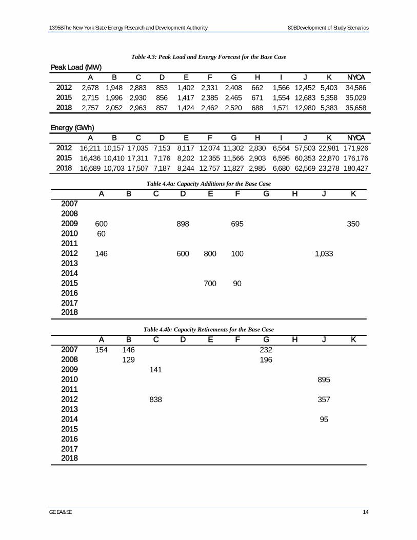
The Base Case is meant to portray the most likely system conditions in the future. The Base Case Scenario for this analysis is based on the assumptions used in the NYSERDA State Energy Plan (SEP) “Starting Point Case.” The Starting Point Case is based on the electricity demand forecast used by the NYISO in its 2009 Reliability Needs Assessment (RNA) for purposes of electricity system planning. In the Base Case Scenario, electricity demand is assumed to increase at an average rate of 0.8 percent per year from 2009 to 2018. The RNA load forecast assumed only currently authorized funding levels for energy efficiency programs, which translates into the assumption that approximately 27 percent of the 15-by-15 policy goal associated with the Energy Efficiency Portfolio Standard (EEPS) is achieved. The peak load and energy assumptions for the Base Case are shown in Table 4.3. The generation addition and retirement assumptions for the Base Case are shown in Table 4.4. These assumptions are consistent with those used in the NYSERDA SEP “Starting Point Case.” This case was studied under a regional carbon policy, i.e., no carbon-related costs were assigned to generators that were not in one of the RGGI states.
1395BThe New York State Energy Research and Development Authority 80BDevelopment of Study Scenarios
GE EA&SE 14
Table 4.3: Peak Load and Energy Forecast for the Base Case
Peak Load (MW)A B C D E F G H I J K NYCA
2012 2,678 1,948 2,883 853 1,402 2,331 2,408 662 1,566 12,452 5,403 34,5862015 2,715 1,996 2,930 856 1,417 2,385 2,465 671 1,554 12,683 5,358 35,0292018 2,757 2,052 2,963 857 1,424 2,462 2,520 688 1,571 12,980 5,383 35,658
Energy (GWh)A B C D E F G H I J K NYCA
2012 16,211 10,157 17,035 7,153 8,117 12,074 11,302 2,830 6,564 57,503 22,981 171,9262015 16,436 10,410 17,311 7,176 8,202 12,355 11,566 2,903 6,595 60,353 22,870 176,1762018 16,689 10,703 17,507 7,187 8,244 12,757 11,827 2,985 6,680 62,569 23,278 180,427
Table 4.4a: Capacity Additions for the Base Case
A B C D E F G H J K200720082009 600 898 695 3502010 6020112012 146 600 800 100 1,033201320142015 700 90201620172018
Table 4.4b: Capacity Retirements for the Base Case
A B C D E F G H J K2007 154 146 2322008 129 1962009 1412010 89520112012 838 35720132014 952015201620172018
1395BThe New York State Energy Research and Development Authority 80BDevelopment of Study Scenarios
GE EA&SE 15
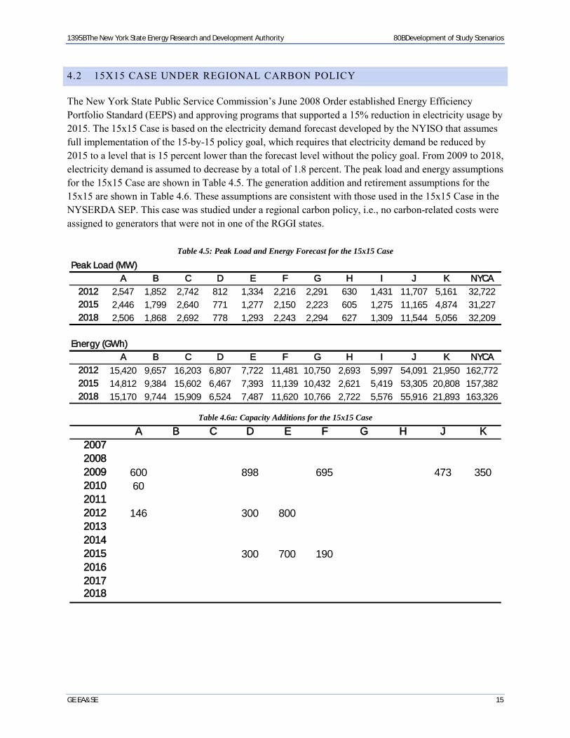
4.2 15X15 CASE UNDER REGIONAL CARBON POLICY
The New York State Public Service Commission’s June 2008 Order established Energy Efficiency Portfolio Standard (EEPS) and approving programs that supported a 15% reduction in electricity usage by 2015. The 15x15 Case is based on the electricity demand forecast developed by the NYISO that assumes full implementation of the 15-by-15 policy goal, which requires that electricity demand be reduced by 2015 to a level that is 15 percent lower than the forecast level without the policy goal. From 2009 to 2018, electricity demand is assumed to decrease by a total of 1.8 percent. The peak load and energy assumptions for the 15x15 Case are shown in Table 4.5. The generation addition and retirement assumptions for the 15x15 are shown in Table 4.6. These assumptions are consistent with those used in the 15x15 Case in the NYSERDA SEP. This case was studied under a regional carbon policy, i.e., no carbon-related costs were assigned to generators that were not in one of the RGGI states.
Table 4.5: Peak Load and Energy Forecast for the 15x15 Case
Peak Load (MW)A B C D E F G H I J K NYCA
2012 2,547 1,852 2,742 812 1,334 2,216 2,291 630 1,431 11,707 5,161 32,7222015 2,446 1,799 2,640 771 1,277 2,150 2,223 605 1,275 11,165 4,874 31,2272018 2,506 1,868 2,692 778 1,293 2,243 2,294 627 1,309 11,544 5,056 32,209
Energy (GWh)A B C D E F G H I J K NYCA
2012 15,420 9,657 16,203 6,807 7,722 11,481 10,750 2,693 5,997 54,091 21,950 162,7722015 14,812 9,384 15,602 6,467 7,393 11,139 10,432 2,621 5,419 53,305 20,808 157,3822018 15,170 9,744 15,909 6,524 7,487 11,620 10,766 2,722 5,576 55,916 21,893 163,326
Table 4.6a: Capacity Additions for the 15x15 Case
A B C D E F G H J K200720082009 600 898 695 473 3502010 6020112012 146 300 800201320142015 300 700 190201620172018
1395BThe New York State Energy Research and Development Authority 80BDevelopment of Study Scenarios
GE EA&SE 16
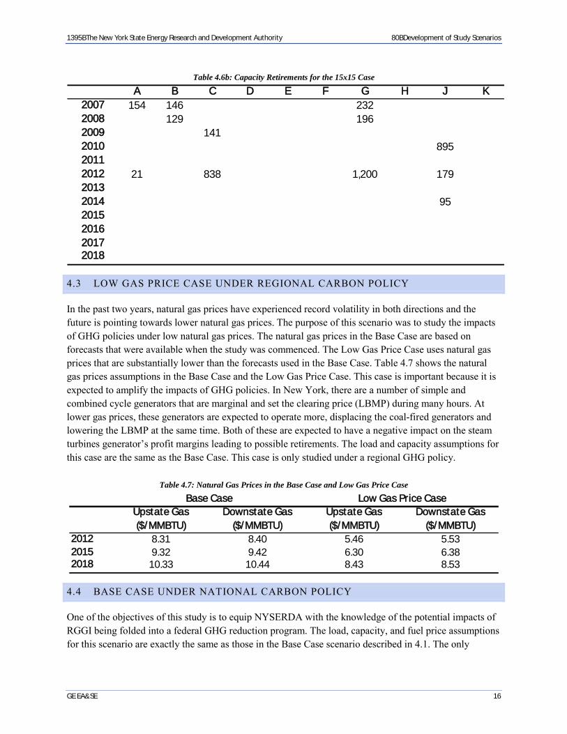
Table 4.6b: Capacity Retirements for the 15x15 Case
A B C D E F G H J K2007 154 146 2322008 129 1962009 1412010 89520112012 21 838 1,200 17920132014 952015201620172018
4.3 LOW GAS PRICE CASE UNDER REGIONAL CARBON POLICY
In the past two years, natural gas prices have experienced record volatility in both directions and the future is pointing towards lower natural gas prices. The purpose of this scenario was to study the impacts of GHG policies under low natural gas prices. The natural gas prices in the Base Case are based on forecasts that were available when the study was commenced. The Low Gas Price Case uses natural gas prices that are substantially lower than the forecasts used in the Base Case. Table 4.7 shows the natural gas prices assumptions in the Base Case and the Low Gas Price Case. This case is important because it is expected to amplify the impacts of GHG policies. In New York, there are a number of simple and combined cycle generators that are marginal and set the clearing price (LBMP) during many hours. At lower gas prices, these generators are expected to operate more, displacing the coal-fired generators and lowering the LBMP at the same time. Both of these are expected to have a negative impact on the steam turbines generator’s profit margins leading to possible retirements. The load and capacity assumptions for this case are the same as the Base Case. This case is only studied under a regional GHG policy.
Table 4.7: Natural Gas Prices in the Base Case and Low Gas Price Case
Base Case Low Gas Price CaseUpstate Gas Downstate Gas Upstate Gas Downstate Gas ($/MMBTU) ($/MMBTU) ($/MMBTU) ($/MMBTU)
2012 8.31 8.40 5.46 5.532015 9.32 9.42 6.30 6.382018 10.33 10.44 8.43 8.53
4.4 BASE CASE UNDER NATIONAL CARBON POLICY
One of the objectives of this study is to equip NYSERDA with the knowledge of the potential impacts of RGGI being folded into a federal GHG reduction program. The load, capacity, and fuel price assumptions for this scenario are exactly the same as those in the Base Case scenario described in 4.1. The only

1395BThe New York State Energy Research and Development Authority 80BDevelopment of Study Scenarios
GE EA&SE 17
difference is that a CO2 allowance price is modeled for all the generators in the Eastern Interconnection, not just those in the RGGI states.
4.5 ECONOMETRIC LOAD CASE UNDER REGIONAL CARBON POLICY
The impacts of any carbon policy, regional or national, will be amplified if the demand grows at a pace that is higher than forecast or if the energy efficiency programs do not produce the intended goals. The Econometric Load case uses a base load forecast from the NYISO Gold book, which was based upon econometric factors and did not include any energy efficiency penetration levels associated with the EEPS proposal. This scenario was studied in both the NYISO RNA and the NYSERDA SEP. In the NYSERDA SEP, this scenario was labeled as “High Demand Forecast” case. The load and capacity assumptions associated with the Econometric Load Case are given in Table 4.8 and 4.9 respectively. This case was studied under a regional carbon policy, i.e., no carbon-related costs were assigned to generators that were not in one of the RGGI states.
4.6 ECONOMETRIC LOAD CASE UNDER NATIONAL CARBON POLICY
This scenario is modeled after the Econometric Load Case described before, but under a federal carbon policy. The CO2 allowance price is modeled for all the generators in the Eastern Interconnection, not just those in the RGGI states. The load and capacity assumptions associated with the Econometric Load Case under the National carbon policy are given in Table 4.8 and 4.9 respectively.
Table 4.8: Peak Load and Energy Forecast for the Econometric Load Case
Peak Load (MW)A B C D E F G H I J K NYCA
2012 2,728 1,984 2,937 869 1,428 2,374 2,454 674 1,623 12,761 5,619 35,4522015 2,810 2,066 3,033 886 1,467 2,468 2,551 694 1,663 13,269 5,801 36,7082018 2,875 2,139 3,090 895 1,486 2,566 2,627 717 1,702 13,673 6,015 37,784
Energy (GWh)A B C D E F G H I J K NYCA
201220152018
16,515 10,349 17,35517,013 10,775 17,91917,404 11,155 18,260
7,2867,4287,499
8,2688,4908,601
12,301 11,51412,787 11,96913,292 12,327
2,8833,0033,109
6,8017,0527,231
58,918 23,901 176,09163,068 24,757 184,26265,803 25,981 190,662

1395BThe New York State Energy Research and Development Authority 80BDevelopment of Study Scenarios
GE EA&SE 18
Table 4.9a: Capacity Additions for the Econometric Load Case
A B C D E F G H J K200720082009 600 898 695 3502010 6020112012 146 600 800 100 1,033201320142015 700 90 75 125201620172018 440 100 769
Table 4.9b: Capacity Additions for the Econometric Load Case
A B C D E F G H J K2007 154 146 2322008 129 1962009 1412010 89520112012 35720132014 952015201620172018
4.7 WORST CASE UNDER REGIONAL CARBON POLICY
It is often customary in a scenario analysis to study the outcome of a policy under a so-called worst-case condition. The Worst Case Scenario in this study was meant to depict future system conditions that wouldlikely lead to most retirements. This case was a combination of the 15x15 caseloads and the natural gas price assumptions from the Low Gas Price Case. It is expected that under these two conditions, steam generators’ revenues will be negatively impacted. This case was studied under the RGGI carbon policy, i.e., no carbon-related costs were assigned to generators that were not in one of the RGGI states. Only theimpacts of high CO2 allowance price were studied under this scenario.
4.8 WORST CASE UNDER NATIONAL CARBON POLICY
This scenario modeled the worst case described before, but under a federal carbon policy. The CO2 allowance price is modeled for all the generators in the Eastern Interconnection, not just those in the

1395BThe New York State Energy Research and Development Authority 80BDevelopment of Study Scenarios
GE EA&SE 19
RGGI states. The load, capacity, and natural gas price assumptions associated with this case are same as those used for studying the regional carbon policy under worst-case conditions.
1395BThe New York State Energy Research and Development Authority 81BEnergy Market Modeling and Simulations of Scenarios
GE EA&SE 20
5 ENERGY MARKET MODELING AND SIMULATIONS OF SCENARIOS
In a deregulated wholesale market, generators recover their short-run marginal costs through the energy market. The net profit earned in the energy market each hour it operates can be calculated from the revenue it earns minus its variable costs of operations including fuel and other variable operations and maintenance costs. The hourly revenue that a unit earns can be approximated as the product of dispatch and the Location Based Marginal Price (LBMP) at its location.
The GE-MAPS production simulation program was used to simulate the operation of the NYISO energy market for the scenarios developed for this study. A production simulation program performs a least-cost dispatch of generators to meet loads on an hourly basis subject to the operational constraints of the generators and the limits of the transmission system. It inherently determines the locational marginal price at every generator and load bus and allows the determination of load payments, generator revenues, and congestion costs. Using the forecast hourly dispatch and prices, the net energy margin for each unit was calculated. In addition, CO2 emissions, energy generation, energy imports, average electricity prices, and cumulative steam units’ net revenue under each scenario were analyzed to determine the impact of the GHG policies. In analyzing the results, the cumulative steam units’ net revenue was used as a proxy for gauging the impact on individual steam units in the system – the likely candidates for retirement under high CO2 prices. The energy market simulation of the scenarios and a description of the major modeling outputs can be found in this section.
5.1 DESCRIPTION OF ENERGY MARKET IN NEW YORK
In New York, the State Public Service Commission (PSC) began restructuring the State’s electric industry in the mid-1990s to promote efficient energy services at just and reasonable rates while providing customers with greater choice, value and innovation. The PSC took a major step toward deregulation by requiring the State’s utility companies to give up their monopoly control of electricity and sell off their power plants to new owners. These new owners now compete with each other in a newly formed wholesale market. The New York Independent System Operator (NYISO) governs this market. Retail competition arrived later. Now the State’s utilities and newly formed energy service provider companies compete with each other to serve consumers through organized retail market.
The New York Independent System Operator (NYISO) operates a multi-settlement wholesale market system consisting of financially binding, day-ahead, and real-time markets for energy, operating reserves, and regulation. The Day-Ahead Market is a forward market in which hourly clearing prices are calculated for each hour of the next Operating Day based on the concept of Location Based Marginal Prices (LBMP). In the Day-Ahead Market, Load Serving Entities submit requests for energy for each hour through Demand Bids. Generation owners submit requests to sell energy for each hour through Supply Offers. These offers can be in the form of a self-schedule or can be in the form of a supply offer where the owner specifies certain prices given specific output levels. The Day-Ahead Energy Market is cleared using Security-Constrained Unit Commitment (SCUC) and Security-Constrained Economic Dispatch (SCED) computer programs to satisfy energy demand bid requirements and supply requirements of the Day-Ahead Energy Market. The results of the Day-Ahead Energy Market clearing include hourly LBMP values, hourly demand and supply quantities, and Scheduled Interchange. The Real-Time Energy Market is a “balancing” market in which the LBMPs are calculated every five minutes, based on NYISO dispatch
1395BThe New York State Energy Research and Development Authority 81BEnergy Market Modeling and Simulations of Scenarios
GE EA&SE 21
instructions and actual system operations. A generator that clears the day-ahead market is paid its hourly scheduled dispatch multiplied by the corresponding hourly LBMP. Deviations from the scheduled dispatch in real-time are settled using real-time LBMPs.
5.2 SIMULATION OF ENERGY MARKET
One of the practical difficulties in studying the impact of emission policies on the transmission system is the sheer scope of analytics involved. The model or software used for this purpose should not only be able to simulate the economics of GHG policies, but also be able to simulate the physical operation of the power system. The fact that GHG policies cannot be studied in isolation for a sub-system, rather the full system due to interdependencies, adds to the complexity of the problem. For example, in order to study the impact of regional and national carbon policies on New York, the rest of the Eastern Interconnection needs to be modeled since New York imports, as well as exports energy to its neighbors. Therefore, it is important to consider a broad enough region to assess accurately and exhaustively, all the impacts of a proposed GHG policy.
In light of the above discussion, the analytical model or software used to study transmission impact must have the following capabilities:
Ability to perform a realistic unit commitment and dispatch taking emissions costs into account Ability to monitor the physical flows on all major transmission lines and corridors, including
transmission interfaces with neighboring systems Ability to model and simulate large power systems without significant approximations
The GE-MAPS production simulation program was used to simulate the operation of the NYISO energy market for the scenarios that were developed in Task 1. The MAPS software simulates the operation of the interconnected utility power system and determines locational marginal prices at all the nodes. The major objective of multi-area production simulation is to model the least cost operation of a power system while ensuring that the system’s security constraints are not violated. Security constraints include the operating limits and capabilities of generation sources, constraints, and contingencies imposed by the transmission system and the operational limits such as minimum operating reserve levels. The market price for electricity is driven primarily by supply and demand, fuel prices, and transmission constraints. The power prices calculated by MAPS represent the incremental cost of generating power at a specific location. Incremental costs include the cost of fuel and variable operations, and maintenance costs, but not fixed costs. Prices determined using this model are conservative estimates of the market prices that would occur in a competitive power market since the model assumes cost-based bids. Additional information about the MAPS software can be found in Appendix B.
The outputs of MAPS include hourly generator dispatch, locational prices, generator emissions and fuel consumption, hourly load-area prices, and hourly flows and shadow prices of transmission interfaces. Based on the hourly output, annual summaries for generators, load-areas, and transmission interfaces can be created. The primary inputs to MAPS are hourly loads, generator capacity and characteristics, fuel prices and transmission constraints that need to be monitored. Sections 5.3 and 5.4 contain more information about the inputs and outputs of the MAPS software.

1395BThe New York State Energy Research and Development Authority 81BEnergy Market Modeling and Simulations of Scenarios
GE EA&SE 22
As mentioned before, the operation of all the generators in the entire Eastern Interconnection (EI) network was simulated for this study. In order to simulate the entire EI, a high-performance computing cluster (HPC) was used. The HPC is a system made up of approximately 100 top-of-the-line servers that allows MAPS to run in a highly parallel environment. Using the HPC, it is possible to partition the MAPS cases into weekly intervals and process each week in parallel on a different CPU. Once all weeks have been simulated, a post processing script allows them to be merged into run-years. It takes approximately two to simulate the hourly operation of all the generators in the EI for one year on the HPC. The post processing procedures required to merge the files takes an additional one-half hour per run-year.
5.3 DATABASE FOR ENERGY MARKET SIMULATION
The EI database consists of the generators in the Eastern Interconnection, their cost and emissions characteristics, loads at the substation level, and transmission lines and limits. The specific load, generation, fuel price and transmission assumptions related to each scenario developed in Task 1 of this study were superimposed on the EI database. The data sources for the underlying EI database are discussed in this section. A more detailed description of the EI database is included as Appendix C.
5.3.1 GENERATION DATA
The EI database contains detailed information regarding thermal, pondage, pumped storage, and renewable generators gathered from various sources. For thermal units, the summer/winter capacities, full load heat rate, and emission rates are obtained from the Ventyx Energy Velocity (EV) Database. Other thermal unit characteristics such as minimum uptime/downtime, start-up costs, variable and fixed O&M costs are based on GE’s assumptions. Pondage Hydro units are modeled using historical monthly energy and the minimum and maximum output rating of the plant. Pumped storage units are modeled using reservoir capacity and the minimum and maximum output rating of the plant. Renewable generation, in particular wind generation, is modeled as hourly load modifiers. For New York wind generators, the hourly load modifier is based on historical, hourly wind generation data by zone. The generator data modeled in GE-MAPS was verified using NYISO’s Gold Book. A more detailed description of the EI database is included as Appendix C.
5.3.2 LOAD DATA
In MAPS, load is modeled by inputting the peak load and energy for each MAPS area (each New York Zone is a MAPS area). The hourly load for each area is calculated by scaling a historical load shape for that area and the input peak load and energy. The GE MAPS program assigns a portion of the hourly load to each load bus in the region based on historical load distribution factors. This is discussed in Appendix C.
5.3.3 TRANSMISSION DATA
The MAPS EI database uses the transmission topology in the 2010 Summer Peak EI load flow case released by the 2005 Multi-Regional Model Working Group (MMWG). In the EI database, all flowgates in the Eastern Interconnection as defined in the North American Electric Reliability Corporation (NERC) Book of Flowgates (BOF) are monitored for overloads. The MAPS database includes the transmission

1395BThe New York State Energy Research and Development Authority 81BEnergy Market Modeling and Simulations of Scenarios
GE EA&SE 23
interfaces (Central East, Total East, etc.) and the limits associated with the first contingencies corresponding to these interfaces that are considered by NYISO in committing and dispatching the generators in the system. The database also includes other (n-1) contingencies that affect the commitment and dispatch of units in New York City. In addition, the MAPS database also models several operational procedures that dictate the commitment and dispatch of units in New York State.
5.4 DESCRIPTION OF MAJOR OUTPUTS
The MAPS software determines the locational marginal price at every generator and load bus and allows the determination of load payments, generator revenues, and congestion costs. Using the forecast hourly dispatch and prices for generators, the net energy margin for each generator was calculated. In addition, CO2 emissions, energy generation, energy imports, average electricity prices, and cumulative steam units’ net revenue under each scenario were analyzed to determine the impact of the GHG policies. In analyzing the results, the cumulative steam units’ net revenue was used as a proxy for gauging the impact on individual steam units in the system – the likely candidates for retirement under high CO2 prices. The major outputs from the energy simulation are described in more detail below.
RGGI States’ Annual CO2 Emissions (tons) – The annual CO2 emissions of the RGGI states include the CO2 emissions from power plants in the following 10 states: Connecticut, Delaware, Maine, Maryland, Massachusetts, New Hampshire, New Jersey, New York, Rhode Island, and Vermont.
New York Annual CO2 Emissions (tons) – The annual CO2 emissions from all the power plants in New York State.
New York State Generation (GWh) – The annual generation (GWH) from all the power plants in New York State.
New York State Load (GWh) – The annual demand (GWh) in New York State.
New York State Imports (GWh) – The annual energy imports (GWh) from neighboring regions, i.e., Pennsylvania Jersey Marland (PJM), ISO New England, Hydro Quebec and Independent Electric System Operator (IESO) of Ontario.
New York State Annual Average Spot Price ($/MWh) – The annual average spot price ($/MWh) is the weighted average zonal LBMP for the 11 New York ISO zones.
New York State Steam Units Cumulative Net Revenue ($) – The cumulative net revenue of all the steam turbine generators in New York State used as a proxy for determining the impact of the different GHG policies on the profitability of generators.
New York State Limiting Interfaces – The flows (GWh) and limiting hours for all the bulk transmission interfaces in New York.
In addition to the system-level outputs described above, MAPS was also used to calculate the net energy market revenue for all the generators in New York. The net energy market revenue is calculated as follows:
Net Annual Energy Revenue = Annual Energy Revenue + Uplift – Annual Energy Costs,

1395BThe New York State Energy Research and Development Authority 81BEnergy Market Modeling and Simulations of Scenarios
GE EA&SE 24
Where,
Annual Energy Revenue = Sum (Hourly Generator Dispatch* Hourly Spot Price),
Annual Energy Costs = Sum of Annual Fuel, Start-up, Var. O&M and Emissions Costs
The next section discusses the above outputs for the study scenarios developed in Task 1 of the project.

1395BThe New York State Energy Research and Development Authority 82BAnalysis of Energy Market Simulation Results
GE EA&SE 25
6 ANALYSIS OF ENERGY MARKET SIMULATION RESULTS
This section presents the results of the energy market analysis that was described in Section 5. Before undertaking a study using a simulation model, it is often necessary to perform a benchmark analysis to understand the efficacy of the model and explain the reasons for the gaps between the model results and historical observations. Section 6.1 discusses the results of the MAPS benchmark simulations that were performed as a part of this study. In order to understand the impact of the carbon policies under the various scenarios, one needs to establish a baseline for comparison. A Baseline simulation forecasts the operation of the system in the future assuming that there is no carbon policy in place. Results of the Baseline simulations are presented in Section 6.2. The impacts of the regional and national carbon policies under the scenarios developed in Task 1 of the project are presented in Section 6.3.
6.1 BENCHMARK SIMULATIONS
A MAPS simulation of the year 2007 was performed and compared with actual 2007 results with the aim of benchmarking the database and model used for this analysis. The objective of this exercise was to determine the ability of the MAPS program and the database to produce results that reflect the economic operation of the New York grid and not to perform an exact back cast of the year 2007. The assumptions for the benchmark simulation are given in Appendix C.
Table 6.1 shows a comparison of emissions (in tons) between MAPS and recorded values12. Comparison of simulated and actual zonal generation by unit type from the benchmark simulations can be found in Appendix C. This appendix also contains a comparison of simulated and actual LBMPs by NYISO zones.
Table 6.1: Comparison of MAPS and actual Emissions
MAPS Simulation 2007 Actuals Emissions (tons) Emissions (tons)
NOXSO2CO2
44,000 130,000 47,550,000
50,000115,000
50,000,000 It can be observed that the emissions from the MAPS model match reasonably well with recorded values. It should be reiterated that the MAPS benchmark simulation did not attempt to recreate the exact system conditions (i.e., model inputs) that existed in the year 2007; however, the loads and installed capacity in the model were matched to 2007 historical values.
It should be pointed out that the CO2 emissions obtained from the MAPS simulation should not be equated to actual CO2 emissions for the following reasons:
Bias in Continuous Emissions Monitoring System. There is a well-documented upward bias in the emissions measured by the Continuous Emissions Monitoring System (CEMS) on the order of two-10%. This is due to calibration of calculations that are based on measuring CO2 in parts per million from
12 The values were obtained from a April 2009 NYISO briefing paper titled “New York State Power Plant Emissions 1999-2008.”

1395BThe New York State Energy Research and Development Authority 82BAnalysis of Energy Market Simulation Results
GE EA&SE 26
samples of combustion exhaust gases. It was agreed that five% was a reasonable estimate for bias by stakeholders in the RGGI process. In contrast, MAPS emissions are estimated directly from projected fuel use based on CO2 emission rates expressed in pounds per MMBtu.
Inside the Fence Emissions: CEMS equipment13 in cogeneration facilities measures the CO2 emissions from generators that serve both internal or “inside the fence” loads, as well as external NYISO loads. The MAPS program models the net generation that serves the grid. Hence, the program captures emissions only from the portion of generation that serves the grid.
6.2 BASELINE SIMULATIONS
As mentioned previously, the Baseline simulations model that system under Base Case conditions without any carbon policy in effect. The results of the Baseline analysis are meant to provide results that will help isolate the impact of carbon allowance prices on the system. They also serve as a bridge between historical observations (market prices, generator dispatch etc. that don’t include the impact of a carbon policy and forecast simulation results, which do. The results of the Baseline simulations, along with those from the study scenarios are summarized in Tables 6.2a, 6.2b and 6.2 c.
6.3 DISCUSSION OF ENERGY MARKET SIMULATION RESULTS
This section presents the results from the MAPS simulations that were performed for the scenarios developed in Task 1. Detailed reports and results for each case are also given in Appendix D. Tables 6.2a, 6.2b and 6.2c shows the results for each scenario under low, medium, and high CO2 prices, if applicable, in the columns. This table shows the output described in Section 5.4 for the three study years.
6.3.1 RGGI STATES’ ANNUAL CO2 EMISSIONS
It can be observed that regardless of the scenario, total RGGI emissions are lower when the CO2 allowance prices are higher. For example, in the Base Case Regional Scenario, for the year 2012, CO2 emissions are 136 million tons under the high CO2 allowance price compared to 148 million tons under the low CO2 allowance price. This is due to the fact that under higher CO2 allowance prices, the RGGI states as a whole import more energy from their neighbors. It can also be observed that under any one of the scenarios, RGGI CO2 emissions decrease in 2015 compared to 2012, and then increase by 2018. This is due to two counteracting effects – the impact of load growth and the CO2 allowance price assumptions for the study years. In the period between 2012 and 2015, load grows by nearly 4,000 GWh in the Base Case. Nevertheless, the RGGI CO2 emissions are lower in 2015 due to the higher CO2 allowance price in 2015 when compared with 2012. For example, in the medium CO2 price scenario, CO2 allowance prices increase from $12/ton in 2012 to $26/ton in 2015, more than a two-fold increase. The higher allowance price in 2015 results in more energy imports into the RGGI states offsetting the effect of load growth.
In general, the RGGI states’ CO2 emissions under the national policy are higher than the corresponding scenario with a regional CO2 policy. This is due to the fact that with the national policy, the energy prices across the eastern U.S., are uniformly higher, which reduces any incentives for the RGGI states to import 13 Only generators rating greater than 25MW are required to install CEMS. Therefore reported CO2 emissions do not include the emissions from generators that are smaller than 25MW.

1395BThe New York State Energy Research and Development Authority 82BAnalysis of Energy Market Simulation Results
GE EA&SE 27
energy from their neighbors. From the results, it can be observed that the RGGI states’ CO2 emissions are highest for the Econometric Case under a National CO2 policy. For reference, actual RGGI states’ CO2 emissions in 2006 were approximately 165 million tons. It should be noted that the CO2 emissions from the model could not be directly equated to the actual emissions for the reasons mentioned before.
6.3.2 NEW YORK ANNUAL CO2 EMISSIONS
The CO2 emissions in New York follow the same trend as that of the RGGI states. The Base Case New York CO2 emissions for the year 2012 are approximately 47, 46, and 45 million tons for the low, medium, and high allowance prices cases respectively. For reference, actual New York State CO2 emissions in 2006 were approximately 53 million tons. It should be noted that the CO2 emissions from the model could not be directly equated to the actual emissions.
6.3.3 NEW YORK STATE GENERATION
Consistent with the CO2 emissions in New York State, the annual generation also is reduced at higher CO2 allowance costs. For example, the Base Case generation for the year 2012 is approximately 153, 152, and 151 thousand GWh for the low, medium, and high allowance prices cases respectively. This trend can be observed for the other scenarios studied. The generation under the national policy is higher than the corresponding scenario with a regional CO2 policy. This is due to the fact that, with the national policy, the energy prices across the eastern U.S., are uniformly higher, which reduces any incentives for the RGGI states to import energy from their neighbors. For reference, actual generation in 2006 was approximately 148 thousand GWh.

1395BThe New York State Energy Research and Development Authority 82BAnalysis of Energy Market Simulation Results
GE EA&SE 28
Table 6.2a: Energy Market Impacts of Carbon Policies

1395BThe New York State Energy Research and Development Authority 82BAnalysis of Energy Market Simulation Results
GE EA&SE 29
Table 6.2b: Energy Market Impacts of Carbon Policies (contd.)

1395BThe New York State Energy Research and Development Authority 82BAnalysis of Energy Market Simulation Results
GE EA&SE 30
Table 6.2c: Energy Market Impacts of Carbon Policies (Contd.)

1395BThe New York State Energy Research and Development Authority 82BAnalysis of Energy Market Simulation Results
GE EA&SE 31
6.3.4 NEW YORK STATE IMPORTS
Under the scenarios that model a regional carbon policy, energy imports are starkly higher than historical values, especially when the CO2 allowance prices are high. This is due to the cost of supply in New York being significantly higher compared to supply in states that do not have a carbon policy, incenting higher imports. For example, in the Base Case with regional carbon policy, energy imports in New York State are approximately 20, 24, and 27 thousand GWh respectively for the low, medium, and high CO2 cases, for the year 2018. Under a national policy, New York imports are comparable to historically observed values. This is due to the fact that energy is uniformly expensive in all the Eastern Interconnection states under this policy; therefore, imports remain substantially the same. For example, in the Base Case with National carbon policy, the 2018 energy imports in New York State are approximately 18 thousand GWh for the low, medium, and high CO2 cases, comparable to historical imports.14
6.3.5 NEW YORK STATE ANNUAL AVERAGE SPOT PRICE
Several different spot price trends can be observed in analyzing the results of the scenario simulations. As the price of CO2 allowance increases, so do energy prices. This is because of the fact that generation owners will include the cost of emission allowances in their bids. The increase in energy prices is more pronounced in the out simulation years (2015 and 2018) as the CO2 allowance costs also increase in those years. Even without any CO2 costs present, price increases can be seen over the study period due to an increase in load growth. Consistent with other results discussed before, the energy prices under the national policy are higher than those with regional carbon policy for corresponding scenarios. Since there is a decrease in the amount of lower priced energy available for import, the energy prices are higher in the National CO2 Case over the Regional CO2 Case. Energy prices in the near-term in the 15x15 case are similar to those in the Base Case; however, energy prices in the out years are lower due to the full impact of the 15x15 EEPS. For the 2018 study year, the average energy price in New York State is approximately 66 and 71 $/MWh respectively with the low and medium CO2 allowance costs in the 15x15 EEPS case. For the same study year, average energy price in New York State is approximately 72 and 78 $/MWh respectively with the low and medium CO2 allowance costs in the Base Case.
6.3.6 NEW YORK STATE STEAM UNITS’ CUMULATIVE NET REVENUE
The cumulative coal and oil-fired steam units’ net revenue was used as a proxy for gauging the impact on individual steam units in the system – the likely candidates for retirement under high CO2 prices. The results show that the cumulative net revenue of New York Steam15 units’ decreases as the CO2 allowance cost increases. This is because the operating costs of these units are higher, making them less profitable. The cumulative net revenues for steam units for the Base Case are approximately $540, $491, and $449 million for the low, medium and high CO2 allowance costs cases in 2012. For, the study year 2015, the cumulative net revenues for steam units are approximately $556, $420, and $377 million for the low, medium, and high CO2 allowance costs. The drop in the cumulative revenue as you go from low to high CO2 allowance prices is amplified in 2015 when compared with 2012 because of the higher allowance
14 For example, imports into New York were roughly 17 GWh in 2007 15 Steam units here refer to coal and oil-fired steam units.

1395BThe New York State Energy Research and Development Authority 82BAnalysis of Energy Market Simulation Results
GE EA&SE 32
prices in 2015. The cumulative net revenue for steam units is the lowest in the Worst Case. In this case, the load growth is lower compared with the Base Case. Also, the gas prices are lower when compared with the Base Case. Due to these two facts, steam units operate less, earning lower revenues.
It should be mentioned that the steam units’ cumulative net revenue was only used as a gauge of the overall impact of carbon policies under the various scenarios. The net energy market revenue for each generator was calculated for all the scenarios studied in this project. This net energy revenue, along with the capacity market revenue,e was used to determine the viability of the unit.
6.3.7 NEW YORK STATE LIMITING INTERFACES
All of the scenarios show an increase in congestion on Central East, Total East, and UPNY-SENY interfaces due to increased West to East to South flows. The increase in North to South flows from 2012 to 2108 primarily due to increased imports from Hydro Quebec (HQ) and increased generation in upstate New York due to Besicorp Empire generation and higher renewable generation in zones A through E. A comparison of the results for the study years 2012, 2015, and 2018 for the low, medium, or high CO2 allowance cost cases shows the following:
Increasing West to East flows from 2012 to 2018 due to increased renewable generation in zones A through E
Increasing North to South flows from 2012 to 2108 primarily due to increased imports from HQ and increased generation in upstate NY due to Besicorp Empire generation and higher renewable generation in zones A through E
Decreasing flow into Long Island from NY due to Neptune HVDC and Caithness CC in the near-term and more expensive units operating in Long Island in the long-term
Detailed discussion of the results for each scenario is included in Appendix D.
1395BThe New York State Energy Research and Development Authority 83BForecasting of New York Capacity Prices
GE EA&SE 33
7 FORECASTING OF NEW YORK CAPACITY PRICES
Since generators are only able to recover their variable costs in the New York energy market, the capacity market provides a mechanism by which a generator can recover some of its fixed operations and maintenance costs in order to stay in operation. It is known that in a competitive market, a generator would attempt to recover its net going-forward costs16 in the capacity market. This assumption is used to derive the supply curve for each locality or capacity zone in the NYISO. Section 7.1 gives additional information about the capacity market run by the NYISO. Section 7.2 describes the simulation of the capacity market using the supply curves derived from the net going-forward costs. Section 7.3 contains a discussion of the capacity market simulation results.
7.1 DESCRIPTION OF CAPACITY MARKETS
The NYISO operates the capacity market to ensure that sufficient capacity is available to reliably meet New York’s planning reserve margins. The NYISO uses the Installed Reserve Margin (IRM) requirement, which is the amount of reserves necessary to meet the reliability standards in New York (16.2% in 2009), in conjunction with the annual peak load forecast to calculate the Installed Capacity (“ICAP”) requirement for the New York Control Area. In addition, the NYISO also determines the locational ICAP requirements for New York City and Long Island since these areas are transmission constrained. The NYISO then converts the ICAP requirements for New York City (NYC), Long Island (LI), and Rest of State (ROS) into Unforced Capacity (UCAP) requirements by using the corresponding location-wide forced outage rates.
The obligations to satisfy the UCAP requirements are allocated to the Load Serving Entities (LSEs) in proportion to their annual peak load in each area. Load Serving Entities can satisfy their UCAP requirements by contracting for capacity bilaterally, by self-scheduling, or by purchasing in the NYISO-run auctions. The NYISO conducts three UCAP auctions: a forward strip auction where capacity is transacted in six-month blocks for the upcoming capability period, a monthly forward auction where capacity is transacted for the remaining months of the capability period, and a monthly spot auction. A generator that clears one of the auctions is paid its unforced capacity times the auction-clearing price for the area in which it is located.
The processes used by the NYISO to determine how much capacity needs to be procured by the various LSEs, is included in Appendix E for reference. This appendix also contains information about the use of demand curves in the spot auction run by the NYISO.
7.2 SIMULATION OF THE CAPACITY MARKET
The capacity price for a locality is determined by the intersection of the supply and demand curves in the spot auction. In order to forecast the capacity prices, the supply and demand curves for each locality needs to be developed for the study year. As mentioned in Appendix E, the demand curve for a locality is constructed using the Net Cost of New Entry (Net-CONE) value and the Unforced Capacity (UCAP) 16 The net going-forward cost for each unit is its going-forward costs minus its net energy market revenue. Going-Forward Costs are the costs that could be avoided if a unit is “mothballed” rather than being kept in service and used to provide capacity. Going forward costs are explained in Appendix F.

1395BThe New York State Energy Research and Development Authority 83BForecasting of New York Capacity Prices
GE EA&SE 34
requirement for the locality. The UCAP requirement for NYCA is derived from the peak load forecast and the IRM requirements. The UCAP requirement for NYC and LI depend on the Locational Capacity Requirements (LCR) requirements for these localities. All the parameters associated with the development of a demand curve (namely, Net CONE, Peak Load, IRM, LCR etc.) can be reasonable estimated for the study years. The more difficult task is the one of developing the supply curve for each locality.
In a competitive market, a unit would attempt to at least recover its going-forward costs from the energy and capacity markets. It can then be assumed that a unit would bid, at minimum, its net going-forward costs (i.e., going-forward cost minus net energy revenues) into the capacity market. This assumption is used to derive the supply curve for each locality. Going-Forward Costs are the costs that could be avoided if a unit is “mothballed” rather than being kept in service and used to provide capacity. Going-forward costs include a portion of the O&M labor, parts and contractual services, administrative and general costs, and insurance. Going-forward costs were estimated to be approximately 75% of the fixed O&M costs. Detailed information regarding going-forward costs is included in Appendix F. The net going-forward cost for each unit is its going-forward costs minus its net energy market revenue. The net energy market revenue for each unit was obtained from the MAPS simulation performed under Task 2 of this project.
The dynamics of the capacity markets in the Northeast are greatly intertwined. The New York capacity market is influenced by neighboring capacity markets, namely New England Forward Capacity Market (FCM) and the PJM Reliability Pricing Market (RPM). In forecasting the capacity prices in New York, these dynamics were taken into account. Based on NYISO’s External Rights Availability, the amount of capacity that can be transacted between New York and its neighbors (ISO New England, Pennsylvania Jersey Maryland, Hydro Quebec, and Independent Electric System Operator) were determined for the study years. This sets the upper and lower bounds for the capacity that can be transacted between New York and its neighbors. The actual capacity transacted will depend on the all the markets reaching equilibrium with respect to each other, subject to import/export limits and the transmission costs associated with selling capacity between markets. For example, if capacity prices were lower in New York ROS capacity market, generators from New York would bid into the ISO-NE capacity market until prices equalize or exports limits are reached. In this analysis, separate supply-demand curves were set up for ISONE and PJM to determine capacity prices in the respective markets. A wheeling rate was assumed between PJM and NYISO to reflect the transmission costs associated with selling energy between the two markets. No wheeling rate was assumed between ISONE and PJM to reflect the seams agreement between the two markets.
Another interesting aspect is how prices in New York City (NYC) locality are determined. In advance of each Obligation Procurement Period, the NYISO calculates the clearing price that would prevail if all qualified capacity in the NYC locality were sold, and establishes that price as the reference level for each mitigated unit. The suppliers in NYC will be required to offer the resources into the spot capacity market at or below its reference level17. The actual market-clearing price for NYC will be close to the reference level due to the limited amount supply that can participate in this market. In the simulation model, NYC capacity prices are determined as the clearing price that would prevail if all qualified capacity in the NYC Locality were sold. The capacity price for LI and ROS are determined based on the intersection of the
17 NYC mitigation rules are explained in Appendix E.

1395BThe New York State Energy Research and Development Authority 83BForecasting of New York Capacity Prices
GE EA&SE 35
supply-demand curves for these two localities. The capacity price for LI is set to be the higher of LI and ROS capacity prices.
In addition to internal generator resources, Special Case Resources (SCRs) can participate in the NYISO capacity market. The NYISO 2009 RNA report was used to obtain an estimate of SCRs in the different localities for the study years. A spreadsheet model using the supply and demand curves defined above was used to determine the cleared capacity and capacity price for each New York locality for the study years. The results of the model are discussed in Section 7.3. The capacity market revenue for a generator that clears the auction is determined as the product of capacity price and the unforced capacity rating of the generator.
7.3 DISCUSSION OF CAPACITY MARKET SIMULATION RESULTS
Table 7.1 gives the summer and winter capacity prices for the three localities under the Base Case scenario for all three study years. For reference, the most recent winter strip auction (November 2008 to April 2009) resulted in a price of 1.77, 2.79 and 1.77 $/KW-month for ROS, NYC and LI respectively. The most recent summer strip auction (May 2009 to October 2009) resulted in a price of 3.01, 6.75 and 3.01 $/KW-month for ROS, NYC and LI respectively.
From table 7.1, it can be observed that the summer prices for all three localities are forecast to be higher than the winter prices. This is due to the fact that the available capacity is lower in summer (due to capacity deration), although the same demand curve is used for the summer and winter auctions. Also, it can be observed that there is a price separation between ROS and NYC localities. The capacity price in NYC is determined by projecting the supply on the demand curve as explained before. The forecast price for New York City is higher than historical values due to demand growth and retirement of a large oil-fired generator. The prices in ROS are higher than historical values because of the influence of neighboring capacity markets. As mentioned before, prices in ROS reach equilibrium with the prices in PJM and ISONE subject to transmission limits and transmission costs between these regions. The capacity prices in PJM (East) are expected to be higher due to a shortage of supply in this region. The capacity prices in ISO-NE are also expected to be higher at least in the short-term, due to a floor price in the ISONE Forward Capacity Market (FCM) Auction. The ROS capacity prices are higher than historical values since they are primarily set by exports into ISO-NE.18
Table 7.2 shows the summer and winter capacity prices for the three localities under the 15x15 scenario for the study years. In general, the capacity prices under this scenario are lower than the base case due to lower load growth assumptions in the 15x15 case.
The prices shown for both the Base Case and the 15x15 Case are valid under the low, medium, and high CO2 allowance prices. Although the CO2 allowance prices have an impact on the net energy revenue and ultimately the supply curve, the capacity prices for under all these CO2 prices are virtually the same since they are set by either projecting the supply on the demand curve in NYC or by exports in ROS. Also, it should be noted that the capacity price forecasts for the Low Gas Price Scenario and the Econometric
18 Even though there is a price separation between NY and PJM capacity markets, the transmission wheeling costs prevent significant exchange of capacity between the two markets. Since there are no wheeling costs between NY and ISONE, New York exports more capacity to ISONE.

1395BThe New York State Energy Research and Development Authority 83BForecasting of New York Capacity Prices
GE EA&SE 36
scenario are virtually the same as the Base case. The capacity price forecasts for the Worst Case Scenario are same as the 15x15 case.
Table 7.1: Capacity Price ($/KW-month) Forecasts for the Base Case
Summer Winter2012 2015 2018 2012 2015 2018
Rest of State 4.44 3.62 3.94 1.60 1.24 1.19New York City 8.20 11.54 14.98 1.72 3.66 4.70Long Island 4.44 3.62 3.94 1.67 1.67 1.67
Table 7.2: Capacity Price ($/KW-month) Forecasts for the Base Case
Summer Winter2012 2015 2018 2012 2015 2018
ROS 4.40 3.28 3.87 1.62 1.26 1.27NYC 7.98 4.29 8.21 1.75 1.65 1.75LI 4.40 3.28 3.87 1.64 1.47 1.55
In general, based on the simulation of the New York capacity market, it can be expected that generators will earn more revenues from the capacity markets than in the past. The capacity prices for all three localities (NYC, LI, and ROS) are expected to be higher, somewhat offsetting the losses in the energy market due to any carbon policy. The capacity revenue, along with the energy market revenue, plays a significant role in determining the viability of the unit.
Many study efforts in the past have focused on determining the viability of generators solely based on energy market revenues. This may lead to erroneous conclusions since the revenues from the capacity markets play a significant role in the viability of generators. This is one of the key findings of the study.

1395BThe New York State Energy Research and Development Authority 84BAnalysis of Retirements due to Carbon Policies
GE EA&SE 37
8 ANALYSIS OF RETIREMENTS DUE TO CARBON POLICIES
In order to determine the impact of GHG policies on the reliability of New York State, it was necessary to identify generators that might mothball or retire if it became economically unviable for them to operate. It was assumed that a generator would continue to operate as a capacity resource as long as it earned enough income from the energy and capacity markets, to cover all its fixed operations and maintenance costs in addition to covering its variable costs. Retrofitting emission control technologies or repowering was not considered as viable options since the primary objective of this study is to evaluate the near-term, worst-case reliability of the system. Section 8.1 discusses the retirement analysis methodology in detail. Section 8.2 presents the results from the retirement analysis.
8.1 RETIREMENT ANALYSIS METHODOLOGY
In order to determine the impact of Green House gas (GHG) policies on the reliability of New York State, it is necessary to identify generators that might mothball or retire if it became economically unviable for them to operate. It can be assumed that a generator will continue to operate as a capacity resource as long as it earns enough income to cover all its fixed operations and maintenance (O&M) costs in addition to covering its variable costs. A generator that is not able to recover all its fixed O&M costs for multiple years into the future will likely retire. A generator that is not able to recover all its fixed O&M costs only in the near-term, but is able to do so in the long-term, may operate, or mothball in the near-term. The generator will operate as a capacity resource in the near term as long as its Net Income is greater than its Going Forward Costs in the near-term. If not, it will mothball.
The calculation of net Income for a generator (Income after tax, before debt principal and interest payments and Fixed O&M Costs) used in the determination of retirements is given in Appendix G. The fixed O&M costs are all the costs that are incurred by a power plant regardless of how much energy it produces. The components of a generator’s fixed cost are described in Appendix G. Going forward costs are the costs that could be avoided if a unit is “mothballed” rather than being kept in service and used to provide capacity. Going forward, costs do not include site leasing or land ownership costs, or property taxes. When a unit is mothballed, the land and physical facilities are maintained so that the option of returning the unit to service is preserved. A detailed description of going forward costs can be found in Appendix F.
Using the methodology described above, generating units that were likely to retire were identified for the three study years, namely 2012, 2015, and 2018. Based on the unit’s retirement status determined for each study year, the availability of the unit for the entire study period was determined using the retirement logic presented in Table 8.1. For example, if the Net Income and Fixed O&M costs of a unit were such that it needed to be (i) retired in 2012, (ii) operating (not retired) in 2015 and (iii) retired in 2018, then the retirement logic would indicate that this will not be available for all three study years (Row 6).
If on the other hand, the Net Income and Fixed O&M costs of a unit were such that it needed to be (i) Operating (not retired) in 2012, (ii) retired in 2015 and (iii) operating (not retired) in 2018, then the retirement logic would indicate that the net income be compared with the going forward cost to determine if the unit will operate or mothball (Row 3) in 2015. As mentioned before, a generator will operate as a

1395BThe New York State Energy Research and Development Authority 84BAnalysis of Retirements due to Carbon Policies
GE EA&SE 38
capacity resource as long as its Net Income is greater than its going forward costs in the near-term. If not, it will mothball.
Table 8.1: Retirement Logic
Row 2012 2015 2018 Retirement Logic1 Not Retire Not Retire Not Retire Available in all three years2 Not Retire Not Retire Retire Unit Not Available in 20183 Not Retire Retire Not Retire check 2015 for mothball4 Not Retire Retire Retire Unit Not Available in 2015, 20185 Retire Not Retire Not Retire check 2012 for mothball6 Retire Not Retire Retire Unit Not Available in 2012, 2015, 20187 Retire Retire Not Retire Unit Not Available in 2012, 2015, 20188 Retire Retire Retire Unit Not Available in 2012, 2015, 2018
8.2 DISCUSSION OF RETIREMENT ANALYSIS RESULTS
For the above analysis, the fixed O&M costs directly related to the power plant such as (i) Labor for routine operations and maintenance, (ii) Routine materials and contract services, (iii) Administrative and general costs, were obtained from a publicly available database. The fixed operations cost related to the location of the power plant such as insurance expense was estimated as given in Appendix G. Going-forward costs or costs that could be avoided if the generator mothballed, include a portion of the O&M labor, parts and contractual services, administrative and general costs, and insurance. Going-forward costs were estimated to be approximately 75% of the fixed O&M costs.
The results of the retirement analysis are given in Tables 8.2a and 8.2b. This table presents the retirement by NYISO super-zones. Super-zones are a combination of the NYISO zones are derived based on transmission congestion pattern in the system.
The retirements in the Base Case ranged from 200 MW in 2012 to around 650 MW in 2018. The maximum retirements were from the Worst Case scenario, which assumed low load growth and low gas prices. In this case, nearly 1400 MW of generators were identified for retirement for the year 2018, out of which nearly 1250 MW of capacity was from coal-fired steam units with an average age of 50 years.
It is interesting to note that even under the Worst Case Scenario (low gas price, low load growth and high CO2 price), the total expected retirements are below 1500 MW in the year 2018. This is primarily due to the robust forecast of capacity market prices in New York as described in Section 7. Many owners whose generators that make little or no revenue from the energy market under the Worst Case conditions are still able to put off retirement decisions due to the high capacity prices.

1395BThe New York State Energy Research and Development Authority 84BAnalysis of Retirements due to Carbon Policies
GE EA&SE 39
Table 8.2a: Generator retirements by Super Zone 2012
Super Zone
Base Case Regional Low CO2
Base Case Regional Med. CO2
Base Case Regional High CO2
15x15 Case Regional Low CO2
15x15 Case Regional Med. CO2
Low Gas Case Regional Low CO2
Low Gas Case Regional Med. CO2
ABCDEFGHIJKNYISO
000
197197
000
197197
000
197197
000
197197
000
197197
0008686
0008686
2015
Super Zone
Base Case Regional Low CO2
Base Case Regional Med. CO2
Base Case Regional High CO2
15x15 Case Regional Low CO2
15x15 Case Regional Med. CO2
Low Gas Case Regional Low CO2
Low Gas Case Regional Med. CO2
ABCDEFGHIJKNYISO
00
121180301
430
121180345
2470
121180548
870
121222430
2140
121222557
00
12170191
2040
12163388
2018
Super Zone
Base Case Regional Low CO2
Base Case Regional Med. CO2
Base Case Regional High CO2
15x15 Case Regional Low CO2
15x15 Case Regional Med. CO2
Low Gas Case Regional Low CO2
Low Gas Case Regional Med. CO2
ABCDEFGHIJKNYISO
00
121180301
430
121180345
2910
121180592
870
121222430
2140
121222557
870
121180389
2470
121180548

1395BThe New York State Energy Research and Development Authority 84BAnalysis of Retirements due to Carbon Policies
GE EA&SE 40
Table 8.2b: Generator retirements by Super Zone (contd.) 2012
Super Zone
Base Case National Low CO2
Base Case National Med. CO2
Base Case National High CO2
Econ. Case Regional Med. CO2
Econ. Case Regional High CO2
Econ. Case National Med. CO2
Econ. Case National High CO2
Worst Case Regional High CO2
Worst Case National High CO2
ABCDEFGHIJKNYISO
00000
00000
00000
00000
00000
00000
00000
000
197197
000
197197
2015
Super Zone
Base Case National Low CO2
Base Case National Med. CO2
Base Case National High CO2
Econ. Case Regional Med. CO2
Econ. Case Regional High CO2
Econ. Case National Med. CO2
Econ. Case National High CO2
Worst Case Regional High CO2
Worst Case National High CO2
ABCDEFGHIJKNYISO
430
121141305
00
121141262
1270
121141389
1060
121134361
2330
121134488
1060
121134361
1060
121134361
68755121222
1,085
1,02755121222
1,425
2018
Super Zone
Base Case National Low CO2
Base Case National Med. CO2
Base Case National High CO2
Econ. Case Regional Med. CO2
Econ. Case Regional High CO2
Econ. Case National Med. CO2
Econ. Case National High CO2
Worst Case Regional High CO2
Worst Case National High CO2
ABCDEFGHIJKNYISO
430
121141305
00
121141262
1270
121141389
1060
121134361
2330
121134488
1060
121134361
1060
121134361
68755121222
1,085
1,02755121222
1,425

1395BThe New York State Energy Research and Development Authority 85BImpact on Bulk Power System Transfer Limits
GE EA&SE 41
9 IMPACT ON BULK POWER SYSTEM TRANSFER LIMITS
The retirement of a generator may have a negative impact on the bulk power transfer capability of the system. The determination of bulk power system transfer limits requires careful consideration of thermal, voltage and stability limitations. The NYISO performs thermal transfer, voltage, and transient stability analyses to determine the transfer limits of bulk transmission interfaces in accordance with New York State Reliability Council (NYSRC) thermal, voltage, fault duty, and stability assessment criteria. A pictorial representation of the NYISO bulk transmission interfaces is given in Appendix H.
First, the NYISO determines the thermal transfer limits of the bulk power interfaces for normal and emergency transfers, such that no facility is loaded beyond its Long-Term Emergency (LTE) and Short-Term Emergency (STE) ratings respectively, following the design criteria specified by NYSRC. Secondly, the NYISO determines the transfer level of interfaces such that no bus voltage falls below its post-contingency low voltage limit or rises above its post-contingency high voltage limit under normal and emergency transfers. For those interfaces where interface power transfer levels may be constrained by voltage considerations, the NYISO also determines the transfer level corresponding to the tip of the nose curve (Voltage versus Interface Transfer Level). To ensure that a voltage-based transfer limit is determined with a safe margin, the lower of the two power transfer levels from the foregoing comparison is selected as the interface transfer limit. Finally, in order to ensure that the system is stable after a contingency, NYISO determines the angular stability limits of interfaces for normal and emergency transfer using NYSRC guidelines. The transfer limit for a transmission interface is the lower of corresponding thermal, voltage and stability limits.
In order to determine the exact impact of a generator retirement on the transfer limits, the above-mentioned analysis are required. Still, an estimate of the impact can be obtained from prior planning and operational studies. The NYISO reviewed the retirement assumptions behind the scenarios and suggested changes to the bulk transfer limits based on their operational experience. This section presents NYISO’s recommendation regarding transfer limit changes. It is to be pointed out that each scenario has different capacity addition and retirement assumptions to begin with. Therefore, even before determining the impact of the identified retirements due to carbon policies, the transfer limits have to be adjusted to reflect the capacity assumptions in each scenario.
It should be noted that not all the scenarios were selected for the transfer limit and reliability analyses. For the purpose of these two analyses, there are only three cases that need to be analyzed. This is due to the fact that here are only three different load conditions that the all the scenarios model – Base Case, 15x15 Case and the Econometric Load Case. For example, the Base Case Regional, Base Case National and the Low Gas price Cases all have the same load, generation and transmission assumptions. There is no need to study the impact of all these cases on the reliability. Since the objective is to determine the worst-case reliability, the reliability analysis is limited to only the scenario (for each study year) that results in the most retirements.
The impact of transfer limit changes due to the generator retirement assumptions in the Base Case, 15x15 Case, and the Econometric Case are discussed in Sections 9.1, 9.2 and 9.3 respectively. Section 9.4 discusses the impact of the retirements due to carbon policy for all of the above-mentioned scenarios.

1395BThe New York State Energy Research and Development Authority 85BImpact on Bulk Power System Transfer Limits
GE EA&SE 42
9.1 BASE CASE TRANSFER LIMIT IMPACTS
The Base Case scenario assumes that 838MW retire in ZoneA by 2012. NYISO’s review showed that the retirement of 838MW in Zone A was expected to impact bulk power system transfer limits. Per the Central East operating nomograms, the Central East and Total East transfer limits were reduced by 75 MW when these megawatts came offline.
9.2 15X15 CASE TRANSFER LIMIT IMPACTS
The NYISO determined that only two of the retirements assumed in the 15x15 case are expected to impact the bulk power system transfer limit. They include 838mw in Zone A and 1200MW in Zone G. Per the Central East operating nomograms, the Central East and Total East transfer limits were reduced by 75MW when 838MW were unavailable in Zone A.
The NYISO 2009 RNA MARS model already includes a dynamic interface rating for the UPNY-Con Ed interface based on the loss of up to 1200 MW in Zone G. This nomogram reduces the UPNY- ConEd interface by 300MW for the loss of 600MW of capacity in Zone G and an additional 300MW for the loss of 1200MW of capacity in Zone G. For the 15x15 Case, this nomogram was expanded to include the loss of up to nearly 2400MW with a reduction of the UPNY-Con Ed interface by 300MW per 600MW of retirements, for up to 2400MW of retirements in Zone G.
9.3 ECONOMETRIC CASE TRANSFER LIMIT IMPACTS
The Econometric load scenario assumes that the 838MW are retired from ZoneA. Per the Central East operating nomograms, the Central East and Total East transfer limits were reduced by 75 MW when this occurred. In addition, based on the analysis completed in the NYISO 2009 RNA study for the High Economic Growth and Extreme Weather scenario, the following additional transfer limit modifications were included due to the high load growth assumed in this case:
West Central is reduced by 200MW
Central East and Total East are reduced by 75MW (This reduction is in addition to the 75MWreduction due to the retirement of 838MW in Zone A)
Dunwoodie is reduced by 350MW
9.4 TRANSFER LIMIT CHANGES DUE TO RETIREMENTS
The NYISO also reviewed the generator retirements identified in this study for the Base Case, 15x15 and Econometric Load Scenarios due to the carbon policies. NYISO expects some of these retirements to cause local voltage problems. Still, for the purposes of this study, it is assumed that the local Transmission Owners would address any voltage impacts due to the plant retirements identified in this study. Therefore, no analysis was performed by the NYISO or GE EA&SE to determine the voltage impact of these retirements and no additional modifications to transfer limits were included. It is assumed that the impacts of these retirements will be localized and will not affect the bulk transmission capability of the system.

1395BThe New York State Energy Research and Development Authority 86BImpact on Power System Reliability
GE EA&SE 43
10 IMPACT ON POWER SYSTEM RELIABILITY
The reliable supply of electric services within the New York Control Area (NYCA) depends on adequate and dependable generation and transmission facilities. In Task 6 of the study discussed in the previous section, it was determined that the bulk power system transfer limits will not change due to generator retirements identified in this study. Nevertheless, retirements can also have a direct impact on the reliability, particularly in areas that are transmission constrained and need to maintain a minimum amount of locational capacity. This task discusses the results of the analysis performed to determine the reliability impacts of the identified retirements. Due to the proprietary nature of the database required to study reliability impacts, the New York Independent System Operator performed this study task. Section 10.1 presents a brief description of the determination of the Loss of Load Expectation (LOLE). Section 10.2 presents the results of the reliability analysis performed by the NYISO.
10.1 DETERMINATION OF LOSS OF LOAD EXPECTATION
The reliability of the New York Power system is determined using a probabilistic approach that is part of the Installed reserve Margin (IRM) process. This technique calculates the probabilities of outages of generating units, in conjunction with load and transmission models, to determine the number of days per year of expected capacity shortages. The result of the calculation is termed Loss of Load Expectation (LOLE), which provides a consistent measure of system reliability. The acceptable LOLE reliability level in the NYCA is stated in the NYSRC Reliability Rules. NYSRC Reliability Rule A-R1, Statewide Installed Reserve Margin Requirements, states:
The NYSRC shall establish the IRM requirement for the NYCA such that the probability (or risk) of disconnecting any firm load due to resource deficiencies shall be, on average, not more than once in ten years. Compliance with this criterion shall be evaluated probabilistically, such that the loss of load expectation (LOLE) of disconnecting firm load due to resource deficiencies shall be, on average, no more than 0.1 day per year. This evaluation shall make due allowance for demand uncertainty, scheduled outages and deratings, forced outages and deratings, assistance over interconnections with neighboring control areas, NYS Transmission System transfer capability, and capacity and/or load relief from available operating procedures.
The primary tool used in the probabilistic analysis for establishing NYCA IRM requirements is GE-MARS (Multi-Area Reliability Simulation). This program includes a detailed load, generation, and transmission representation for 11 NYCA zones (A through K), as well as the four external Control Areas (Outside World Areas) interconnected to the NYCA (see appendix H for a pictorial representation of the study system). A sequential Monte Carlo simulation forms the basis for MARS. The Monte Carlo method provides a fast, versatile, and easily expandable program that can be used to fully model many different types of generation and demand-side options. In MARS, the transmission system between interconnected areas is modeled through transfer limits on the interfaces between pairs of areas. Simultaneous transfer limits can also be modeled in which the total flow on user-defined groups of interfaces is limited. Random forced outages on the interfaces are modeled in the same manner as the outages on thermal units, through the use of state transition rates.

1395BThe New York State Energy Research and Development Authority 86BImpact on Power System Reliability
GE EA&SE 44
The MARS program calculates the standard reliability indices of daily and hourly LOLE (days/year and hours/year) and Loss of Energy Expectation (LOEE in MWh/year). The use of sequential Monte Carlo simulation allows for the calculation of time-correlated measures such as frequency (outages/year) and duration (hours/outage). The program also calculates the need for initiating Emergency Operating Procedures (EOPs), expressed in days/
The study procedures used for the 2008 IRM Study are described in detail in NYSRC Policy 5-3, Procedure for Establishing New York Control Area Installed Capacity Requirements19. Policy 5-3 describes the computer program used for the reliability calculation in addition to the procedures and types of input data and models used for the IRM Study.
It should be noted that not all the scenarios were selected for the transfer limit and reliability analyses. For the purpose of these two analyses, there are only three cases that need to be analyzed. There are only three different load conditions that the scenarios model – Base Case, 15x15 Case, and the Econometric Load Case. For example, the Base Case Regional, Base Case National and the Low Gas price Cases all have the same load, generation and transmission assumptions. In addition, these scenarios were studied under different CO2 allowance price assumptions. There is no need to study the impact of all these cases on the reliability. Since the objective is to determine the worst-case reliability, the reliability analysis is limited to only one out the three scenarios (for each study year) that results in the most retirements.
10.2 DISCUSSION OF RELIABILITY RESULTS
The NYISO performed the reliability analysis using the GE Multi-Area Reliability Simulation (MARS) program version 2.92. The reliability analysis was conducted to determine if the assumed capacity modifications and retirements would result in the violation of the Loss of Load Expectation (LOLE) criterion of once in 10 years (or 0.1 per year) as established by the Northeast Power Coordinating Council (NPCC) and the New York State Reliability Council (NYSRC). That criterion establishes that the resources available on the electric system in New York should be sufficient such that the probability of an unplanned disconnection of firm load due to resource deficiencies is never greater than once in ten years.
The NYISO uses the GE-MARS program and an associated database in both the IRM process, as well as the RNA process. Due to the proprietary nature of the databases, they are not available to the public. The NYISO used the RNA database as a starting point for this study. For each of the scenario that needed to be analyzed, the NYISO created a reference case and a change case. The reference case includes all the generation addition and retirement assumptions in a scenario in so far as these assumptions are different from the RNA assumptions. The reference case also includes the transfer limit changes identified in Task 6. The change case includes the retirements identified for each scenario, in addition. The results of the reliability analysis performed by the NYISO are discussed below.
Table 10.1 shows the LOLE for NYCA for the Base Case with and without the retirements identified in Task 5. The retirements do cause the LOLE to increase; however, the LOLE is well below 0.1 indicating that the system is reliable. This is because the Base Case assumes that approximately 27 percent of the 15 by 15 policy goal associated with the Energy Efficiency Portfolio Standard (EEPS) is achieved. The reduced load, in combination with the identified capacity additions, results in a healthy reserve margin 19 NYSRC Policy 5-3 can be found on the NYSRC website: http://www.nysrc.org

1395BThe New York State Energy Research and Development Authority 86BImpact on Power System Reliability
GE EA&SE 45
resulting in a very low LOLE. The NYISO RNA study also identified that with the Base case assumptions; New York will be in an over-supplied situation until 2017.
Table 10.2 shows the LOLE for NYCA for the 15x15 Case with and without the retirements identified in Task 5. As observed in the Base case, LOLE is well below 0.1 in both the cases with and without the retirements due to carbon policies. This is because the 15X15 Case assumes that approximately 100 percent of the 15x15 policy goal associated with the Energy Efficiency Portfolio Standard (EEPS) is achieved. The peak load and energy in the 15x15 Case is nearly 5% below the Base Case for the year 2012 and approximately 10% below the Base Case projections for 2015 and 2018. The reduced load, in combination with the identified capacity additions, results in a healthy reserve margin resulting in a very low LOLE.
Table 10.3 shows the LOLE results for the Econometric Load Forecast case. In this case, the peak load and energy assumptions are from the NYISO Gold Book, without any energy efficiency gains from the EEPS proposal assumed. The peak load and energy in the Econometric Load Case is nearly 3% above the Base Case for the year 2012 and approximately 6% above the Base Case projections for 2015 and 2018. Since the loads are significantly higher when compared with the Base Case, NYCA will have LOLE violations with or without the identified retirements by 2015. The results of this analysis are consistent with the 2009 RNA analysis where NYCA has LOLE violations in 2016/2017 for the same case. It can be seen that without the retirements due to carbon policy, the system is marginally reliable in 2015. However, with these retirements, the LOLE is greater than 0.1, indicating that the system will violate the reliability criterion. In the year 2018, the LOLE for both the case with and without retirements is well above 0.1 days/year. The retirements due to any carbon policy will expedite the violations and make them more severe by 2018. Still, it should be noted that the econometric case portrays a fictitious worst-case scenario in which generation additions do not keep up with the peak load increase due to unrealized efficiency gains.
Table 10.1: Reliability Analysis Summary for Base Case
NYCA LOLE NYCA LOLE NYCA LOLEwithout retirements with retirements Difference
2012 0.003 0.005 0.0022015 0.007 0.021 0.0142018 0.029 0.068 0.039
Table 10.2: Reliability Analysis Summary for 15x15 case
NYCA LOLE NYCA LOLE NYCA LOLEwithout retirements with retirements Difference
2012 0.005 0.010 0.0052015 0.000 0.000 0.0002018 0.001 0.008 0.007

1395BThe New York State Energy Research and Development Authority 86BImpact on Power System Reliability
GE EA&SE 46
Table 10.3: Reliability Analysis Summary for Econometric Load Case
NYCA LOLE NYCA LOLE NYCA LOLEwithout retirements with retirements Difference
2012 0.015 0.015 0.00020152018
0.0990.201
0.1800.297
0.0810.096

1395BThe New York State Energy Research and Development Authority 87BStudy Findings
GE EA&SE 47
11 STUDY FINDINGS
One of the big unknowns when considering the effect of any cap-and-trade emissions policy that covers electricity producers is its impact on the economics and reliability of the electric power grid. A cap-and-trade scheme increases thermal power plants owner’s variable cost of operation by forcing them to buy emissions allowances for each ton of carbon dioxide (CO2) their generating unit emits. The primary objective of this study is to determine the economic and reliability impacts of carbon policies under a range of future system conditions. Based on this study, the following conclusions can be made.
11.1 RELIABILITY IMPACTS
The reliability of the New York system will not be harmed due to a carbon policy under most conditions. With the current EEPS spend, the demand for energy in New York is expected to grow at only 0.8% per year from 2009 to 2018. If the 15x15 goal is fully realized, New York’s demand will actually be reduced by 1.5% from 2009 to 2018. Due to the reduced load, the system will have sufficient generation to result in an LOLE in excess of reliability targets, assuming only known retirements. Although a carbon policy will have a slight negative impact on the LOLE, the system will still be very reliable overall. In the scenario that none of the proposed gains due to EEPS are realized and no additional generators come on-line, the retirements due to any carbon policy will expedite the violations. Still, such a scenario is not likely since the NYISO would maintain the reliability of the system through its Comprehensive Reliability Planning Process (CRPP) and is used only to study the impact of carbon policy under an extreme case.
One of the primary reasons for the system’s reliability not being negatively impacted is that the bulk transfer capability will be maintained in spite of the retirements. It is expected that the impacts of the retirements due to a carbon policy will be localized and will not affect the bulk transmission capability of the system.
The impact on the bulk transmission is not severe because very few generators retire even under worst-case conditions. The maximum retirements were from the Worst Case scenario, which assumed low load growth and low gas prices. In this case, nearly 1400 MW of generators were identified for retirement for the year 2018, out of which nearly 1250 MW of capacity was from coal-fired steam units with an average age of 50 years. The retirements in the Base Case ranged from 200 MW in 2012 to around 650 MW in 2018
The reason for fewer than expected retirements is the robust forecast of capacity market prices in New York. The capacity markets in the Northeast are inter-twined. The neighboring markets prop up the prices in New York. Many of the generators that make little or no revenue from the energy market under the Worst Case conditions are still able to put off retirement decisions due to the high capacity prices.
Nevertheless, energy prices do increase due to the CO2 allowance costs being included in generators’ supply offer. This will be discussed in the next section.

1395BThe New York State Energy Research and Development Authority 87BStudy Findings
GE EA&SE 48
11.2 ENERGY PRICE IMPACTS
Any CO2 policy can in general be expected to lead to higher energy prices. If the CO2 allowances are auctioned, generators will attempt to recover these costs from the energy market by including the costs in their supply offers. At higher CO2 allowance prices, the offers from generators will also be higher, especially from coal-fired steam generators that have higher CO2 emissions. Under a regional carbon policy, this will result in energy being imported into the affected region from the region without a carbon policy. In the Base Case simulations, imports into New York will be higher by 10% and 45% under a low and high CO2 allowance price by the year 2018 when compared to case with no CO2 allowance prices (Baseline Case). As a result, the generation within New York, particularly from coal-fired and oil-fired generators will decrease, impacting their revenues. In the Base Case simulations, cumulative net energy margin of steam units in New York decrease by 16% and 44% under a low and high CO2 allowance price by the year 2018 when compared to a case with no CO2 allowance prices. The LBMP in New York will be higher since the clearing price will be set by gas turbines whose supply offers will include some recovery of the CO2 allowance prices. Under high CO2 allowance prices, the impact on energy prices will be higher. In the Base Case simulations with a regional CO2 policy, energy prices in New York will be higher by 5% and 22% under a low and high CO2 allowance price by the year 2018
Energy price impacts will be muted in the 15x15 Case. Under the 15x15 case, due to the full realization of the EEPS goal, the load will be much lower than the Base Case. The impact of any carbon policy on energy prices is negated by the lower load growth. Similarly, lower gas price will also negate the impact of any carbon policy at a regional level. The LBMP in New York is often set by gas-fired generators. An increase in the offer price of energy due to CO2 allowance price will be offset by a decrease in gas price. An 18 percent decease in gas price from the Base Case assumptions, is likely to lead to a 10% reduction in energy price in the 15x15 case with low CO2 allowance price in 2018.
An interesting finding is that an increase in load that could occur if the EEPS goals are not realized does not have any significant impact on the LBMP in New York. The econometric case assumed a peak load and energy that was approximately 6% higher than the Base Case. Nevertheless, this load increase is not significant enough to change the energy prices in New York. Coal-fired steam units, in fact, operate more and are less likely to retire under this scenario. The cumulative net revenue of steam units is 35% higher in the econometric case with high CO2 allowance cost when compared with the corresponding Base Case for the year 2018. This confirms the earlier finding that the reliability violations in the econometric case is driven more by shortage of installed capacity rather than by retirements due to any carbon policy.
The impacts of a national carbon policy replacing a regional carbon policy are discussed next.
11.3 CO2 EMISSION REDUCTIONS
Based primarily on previous emission history, New York received 64.3 million tons as its CO2 emissions budget. Beginning in 2015, this cap will be reduced by 2.5 percent each year, for a total reduction of 10 percent by 2019. The emission target for 2018 is roughly 59 million tons. The CO2 emissions under all the scenarios obtained from the MAPS simulations are well under this figure. In reality, New York’s CO2 emissions will most likely be below this limit, under all of the scenarios analyzed in this study, even after considering the downward emissions bias in the MAPS program. It is interesting to note that CO2
1395BThe New York State Energy Research and Development Authority 87BStudy Findings
GE EA&SE 49
emissions are below the prescribed limit even in the Baseline Case that assumes no carbon policy. This is due to the impact of partial or complete realization of existing policies such as 15x15 EEPS and 30% RPS goals. Any carbon policy only further accelerates the achievement of the target.
Still, the reduction in CO2 emissions also depends on the reach of the carbon policy. In general, New York will achieve more CO2 reductions sooner under a regional policy than a national policy. Under a regional policy, New York will import more energy from regions that don’t have a carbon policy. If RGGI is folded into a national program, imports into New York will decrease and more energy will be generated in New York by units that are more expensive. As a consequence, energy prices will increase.
In the Base Case scenario, a national carbon policy will result in imports being lower by 12% and 33% with low and high CO2 allowance price assumptions respectively, when compared with the same scenario under a regional carbon policy for the year 2018. At the same time, the energy produced within New York will be one% and six% higher and the energy prices three% to seven% higher than it is with a regional policy, depending on the CO2 allowance prices. CO2 emission under the national program will be four% and 17% higher with low and high CO2 allowance price assumptions respectively, when compared with the same scenario under a regional policy for the year 2018. Nevertheless, as mentioned before, CO2 emissions will still be under the target set by RGGI. CO2 emission reduction will be slower under a national program when compared with a regional program.

1395BThe New York State Energy Research and Development Authority 88BAppendix A MAPSPTMP Software
GE EA&SE 50
12 APPENDIX A MAPS TM SOFTWARE

1395BThe New York State Energy Research and Development Authority 88BAppendix A MAPSPTMP Software
GE EA&SE 51

1395BThe New York State Energy Research and Development Authority 89BAppendix B – EI Database Description
GE EA&SE 52
13 APPENDIX B – EI DATABASE DESCRIPTION
13.1 EASTERN INTERCONNECTION (EI) DATABASE BASE CASE ASSUMPTIONS
The purpose of this document is to describe the key underlying data and input assumptions for the GE-MAPSTM (MAPS) Eastern Interconnection (EI).
13.2 REGION AND CONTROL AREAS WITHIN EI
The Eastern Interconnection is one of the major electrical interconnections of North America. While electrically independent of its neighboring interconnections, the EI is nevertheless connected to the neighboring Quebec, Western, and Texas interconnections either through high voltage direct current (HVDC) ties and/or through variable frequency transformers (VFT). The EI is comprised mostly of the eastern and midwestern portions of the United States and Canada as shown in Figure 1 below.
Figure 1 - Electrical Interconnections of North America
13.3 LOAD FORECASTS, LOAD SHAPES
In general, the EI Database load forecast is based upon data from the North American Electric Reliability Council (NERC) Electricity Supply and Demand (ES&D) database and ISO/RTO data where available. The modeling of load is based on load shapes from FERC Form 714 data, which was extracted from Ventyx Energy Velocity (EV) database and adjusted to be consistent with forecasts of peak and energy.

1395BThe New York State Energy Research and Development Authority 89BAppendix B – EI Database Description
GE EA&SE 53
13.4 FUEL PRICE ASSUMPTIONS
The fuel price assumptions for the EI Database were obtained from forecasts within the EV dataset.
Natural gas and oil price forecast assumptions are based upon the NYMEX futures contracts for Henry Hub (HH) natural gas and West Texas Intermediate (WTI) crude oil. Daily closing prices were averaged by delivery month for each commodity to determine the default natural gas and oil price forecasts for those delivery months. Prices for natural gas at 52 nodes across the EI database were estimated by performing a historical analysis of basis differentials between these nodes and historical HH prices, including Transco Zone 6 Non-NY.
For future years, coal prices by grade are specified for each NERC sub-region modeled in the EI database, based upon EV coal price projections. The EV coal price projections (by grade, by region) are used to calculate an average price ($/MMBtu) for each sub-region within the EI database.
13.5 GENERATING RESOURCES
13.5.1 ENERGY VELOCITYTM DATA
The data for generating resources in the MAPS EI database was obtained from the EV database. Within the EI database, generating resources are represented at the unit level, based on individual unit cost, operations, and performance data from EV. Individual units or facilities with ratings less than 20 MW are generally aggregated into a larger, generic facility located within the geographical area.
For those existing generating resources where plant-specific data (cost, performance, operations, etc.) was publicly available, this data was included.
In the absence of plant-specific data, default assumptions were made using publicly available sources and/or EA&SE estimates. For example, EA&SE applies generating plant operation and performance curves (developed by GE Energy’s Engineering group) for each technology modeled, to estimate the power points and the incremental heat rates associated with each power point. Additional operational performance characteristics and assumptions are developed based upon various studies and analyses prepared by EA&SE:
Minimum Up Time: not currently modeled in MAPS Minimum Down Time: estimates based upon analysis of actual historical data Must Run: currently applies to all gas turbine, conventional hydro, and “RMR” or reliability Start-Up Costs: assumptions are based on GE Contract Services estimates of median costs amortizing
the inspection and maintenance costs over the number of operating hours or startups that would trigger inspections and maintenance
Planned and Forced Outage Rates: based on EA&SE estimates using the NERC Generating Availability Data System (GADS)

1395BThe New York State Energy Research and Development Authority 89BAppendix B – EI Database Description
GE EA&SE 54
13.5.2 MODELING OF COGENERATION/PRIVATE NETWORK UNITS
Cogeneration or “Private Network” resources in the EI database are modeled based on EV dataset, which is based on DOE EIA-860 database. In general, only the amount of capacity that is available to the grid (“Net to Grid”) is modeled in MAPS. The amount of capacity that is designated or contracted to serve the customer’s own load (“Host Load,” “Behind the Fence” or “Behind the Meter”) is not modeled in MAPS, since the load that this capacity serves is not modeled.
13.5.3 MODELING OF WIND RESOURCES
Wind turbine resources are modeled in MAPS using hourly wind generation profiles to more closely reflect the amount and timing of energy available by area. The hourly profiles are based on recent GE studies and assigned to the various wind resources in the EI database, based on the source location (longitude and latitude) of each profile.
13.5.4 MODELING OF HYDRO RESOURCES
Conventional hydro generation resources are modeled in MAPS based on numerical averages of historical monthly generation from 1996 through 2007. Plants are modeled with the following monthly constraints: minimum capacity, maximum capacity, and total volume of available energy. With these assumptions, MAPS seeks to optimize the hydro resource generation and provide regulation and load-following capability.
13.5.5 MODELING OF PUMPED STORAGE HYDRO RESOURCES
In general, pumped storage resources are assumed to an efficiency of 75% (1.33 MWh of pumping energy required to generate 1 MWh of output). MAPS schedules these resources weekly, and each pumped storage plant is assumed to have eight hours of storage available.
13.5.6 DEMAND-SIDE RESOURCES
Firm demand-side resources, including demand response (DR) and load management (e.g., direct load control, load acting as resource, interruptible loads) are included by modeling as load modifier with zero cost. If it is necessary to model specific demand-side resources as a (peaking) generating resource, the cost of such a resource is assumed to be in excess of the most expensive thermal generating resource (gas turbine).
13.5.7 TRANSMISSION & INTERCHANGE
The EI Generation-Transmission data file (GT file) contains assumptions on generating unit location, transmission flow gates and interface limits, line limits, contingencies, and HVDC interconnections and phase shifters. Each generating unit modeled in the EI Database is assigned to the respective generator bus on the EI system, based on the EI load flow data dictionary (CEII) and EV data.

1395BThe New York State Energy Research and Development Authority 89BAppendix B – EI Database Description
GE EA&SE 55
13.6 LOAD FLOW MODELS
The transmission model in MAPS is obtained from a solved AC load flow. The transmission model in the EI Database is based on the 2010 Summer Peak EI load flow case released by the 2005 Multi-Regional Model Working Group (MMWG), which formerly fell under the purview of NERC but currently falls under the purview of the Eastern Interconnection Reliability Assessment Group (ERAG). Additionally, select recently announced transmission projects for NYISO, ISONE, and PJM have been added to the load flows.
13.6.1 TRANSMISSION CONSTRAINTS
The EI Database reflects all transmission interfaces defined within the NERC Book of Flowgates (BOF) as well as selected “New England Potentially Limiting Bulk Transmission Interfaces” as defined in the New England Power Pool (NEPOOL) FERC Form 715 filings. The EI Ddatabase models the flow limits of transmission lines, interfaces, contingencies, Phase Angle Regulators (PARs), and High Voltage DC (HVDC) lines. In addition to the interface limits, the flows across all Phase Angle Regulators (PARs) and High Voltage DC (HVDC) transmission lines in the EI are monitored subject to their capabilities. The EI Database also contains hurdle rates that represent the wheeling and other transactional costs between the various RTOs/NERC regions in the EI.

1395BThe New York State Energy Research and Development Authority 90BAppendix C – GE MAPS Benchmark Simulation
GE EA&SE 56
14 APPENDIX C – GE MAPS BENCHMARK SIMULATION
A benchmark simulation was performed to determine the efficacy of the GE MAPS program and associated database in simulating the operations of the New York energy market. A MAPS simulation of the year 2007 was performed and compared with actual 2007 results. The objective of this exercise was to determine the ability of the MAPS program and the database to produce results that reflect the economic operation of the New York grid and not to perform an exact back cast of the year 2007. As such, no effort was made to exactly replicate the 2007 system conditions in the simulation. Some of the significant changes made to the model are discussed below.
14.1 GENERATION DATA
The EI database discussed in Section 5 was used as a starting point. The 2007 installed capacity in MAPS was verified with the 2007 NYISO Gold Book to ensure that all units were accounted for. Below are some specific changes made to the MAPS model for the benchmark simulation:
Actual 2007 planned maintenance outage periods for nuclear units in NY were modeled. For the remaining thermal and hydro units, the planned and forced maintenance outage periods were determined within MAPS
Niagara Moses unit was modeled using historical hourly generation Zonal gas prices were modeled using actual 2007 Henry Hub gas prices and standard basis
differentials.
14.2 LOAD DATA
2007 peak load and energy by New York zone were input. Still, 2007 actual load shapes were not used. Instead, 2002 load shapes were scaled to meet the 2007 zonal peak load and energy.
14.3 TRANSMISSION DATA
The transmission topology in the EI database was changed to reflect the system conditions in year 2007. Transmission projects that came online partway into the year (for example, Mott Haven), except the Neptune project, were assumed to be online throughout the year in MAPS. Nevertheless, transmission outages were not modeled.
Table C1 shows the generation by zone and by type from the 2007 MAPS benchmark simulation. Table C2 shows the same information for 2007 obtained from the 2008 Gold Book. In general, there is a good match between the two, establishing the ability of the MAPS program and the database to produce results that reflect the economic operation of the New York grid.
It can be observed that MAPS operates coal and combined cycle units slightly more than actuals, at the expense of GTs and Steam-Oil units. This is likely due to the fact that in reality, there may be non-economic reasons (for example, local reliability rules) to dispatch GTs and Steam-Oil units. As far as possible, all of the known operational procedures were modeled in the EI database. Also, as mentioned previously, actual generator and transmission line outages were not modeled in the MAPS database. These outages could also have an impact on the dispatch.

1395BThe New York State Energy Research and Development Authority 90BAppendix C – GE MAPS Benchmark Simulation
GE EA&SE 57
Table C1: 2007 Generation by zone and unit type from MAPS
Zone CC-GAS GT WIND ICICLUMPED UNITS NUCLEAR PONDAGE
PUMPED STORAGE ST-COAL ST-O&G
ST - WASTE TOTAL
A 295 71 29 - 25 - 13,709 - 12,956 - 252 27,337 B 20 0 - - 4 4,683 175 - 1,595 - - 6,477C 1,066 41 264 - 20 20,757 454 - 5,191 2 210 28,004 D 676 27 200 - - - 6,384 - - 65 - 7,352E 13 - 666 - 1 - 2,099 - 414 67 - 3,259F 13,240 - - - 5 - 2,033 750 - - 84 16,113 G - 1 - - 7 - 298 - 4,821 976 56 6,159H - - - - - 15,937 - - - - 369 16,305 J 15,750 433 - - - - - - - 6,349 - 22,532 K 2,780 591 - 28 123 - - - - 5,392 897 9,812
TOTAL 33,840 1,164 1,159 28 186 41,377 25,153 750 24,976 12,851 1,868 143,351
Table C2: 2007 Generation from NYISO Gold Book
Zone CC-GAS GT WIND ICICLUMPED UNITS NUCLEAR PONDAGE
PUMPED STORAGE ST-COAL ST-O&G
ST - WASTE TOTAL
A 316 707 10 111 - - 13,286 - 11,976 - 222 26,642 B 18 77 16 30 - 4,931 180 - 1,222 - - 6,474C 2,557 252 72 197 - 20,882 438 - 3,828 248 227 28,701 D 686 1,404 - - - - 6,378 - - - 136 8,604E 90 - 774 - - - 2,106 - 441 - 120 3,532F 10,860 - - 46 - - 2,089 768 - - 83 13,846 G - 2 - - - - 297 - 3,832 1,704 46 5,881H - - - - - 16,638 - - - - 390 17,028 J 16,072 1,446 - - - - - - - 9,199 - 26,716 K 1,922 1,467 - 32 - - - - - 8,627 935 12,982
TOTAL 32,521 5,355 873 416 - 42,451 24,774 768 21,299 19,777 2,159 150,407
Table C3 shows a comparison of the actual average 2007 NYISO DAM price with that obtained from the MAPS benchmark. The annual average price for NYISO obtained from MAPS is almost the same as the actual price. Nevertheless, MAPS slightly over-predicts the upstate prices and under-predicts the NYC and LI prices. This difference could be possibly due to transmission line outages not modeled in the benchmark database. It could also be due to some of the part-year transmission project such as Mott Haven that are assumed to come online in the beginning of the year in MAPS and due to marginal losses.

1395BThe New York State Energy Research and Development Authority 90BAppendix C – GE MAPS Benchmark Simulation
GE EA&SE 58
Table C3: Comparison of MAPS and actual zonal DAM Prices
Price Node Name 2007 DAM Price ($/MWh) 2007 MAPS Benchmark ($/MWh)
WEST (ZONE A) 53.11 58.94GENESE (ZONE B) 55.28 59.44CENTRL (ZONE C) 59.09 62.70NORTH (ZONE D) 58.94 62.58MHK VL (ZONE E) 61.42 62.93CAPITL (ZONE F) 69.29 67.75HUD VL (ZONE G) 72.23 69.52MILLWD (ZONE H) 73.41 70.98DUNWOD (ZONE I) 73.49 71.16N.Y.C. (ZONE J) 77.18 73.08LONGIL (ZONE K) 86.76 79.25AVERAGE 67.29 67.12
Table C4 shows a comparison of emissions (in tons) between MAPS and recorded values. It can be observed that the emissions from the MAPS model match reasonable well with recorded values.
Table C4: Comparison of MAPS and actual Emissions
MAPS Simulation 2007 Actuals Emissions (tons) Emissions (tons)
NOXSO2CO2
44,000 130,000 47,550,000
50,000115,000
50,000,000

1395BThe New York State Energy Research and Development Authority 91BAppendix D – Energy Market Summaries by Scenario
GE EA&SE 59
15 APPENDIX D – ENERGY MARKET SUMMARIES BY SCENARIO
15.1 BASE CASE UNDER REGIONAL CARBON POLICY
The results of the Base Case under regional carbon policy are discussed below. Table D1 in this appendix shows the study results.
15.1.1 RGGI AND NEW YORK CO2 EMISSIONS
It can be observed that the CO2 emissions in New York, as well as all the RGGI states, decreases as the allowance price for CO2 increases. For the study year 2012, total CO2 emissions in the RGGI states add up to nearly 149, 143, and 137 million tons respectively for the low, medium, and high CO2 case, compared to nearly 154 million tons without any allowance cost associated with CO2. A similar trend can be observed over the longer term, for the year 2018.
New York state emissions are also reduced at higher costs for CO2 allowance. For the study year 2012, total CO2 emissions in New York State adds up to nearly 47, 46 and 45 million tons respectively for the low, medium and high CO2 case, compared to approximately 46 million tons without any allowance cost associated with CO2. Over the longer term, the reduction is more pronounced. For the study year 2018, total CO2 emissions in New York State adds up to approximately 47, 43 and 38 million tons respectively for the low, medium and high CO2 case, compared to nearly 49 million tons without any allowance cost associated with CO2.
15.1.2 NYISO ANNUAL SUMMARY
Consistent with the carbon emission in New York State, the annual generation also is reduced at higher CO2 allowance costs. For the study year 2018, total generation in New York State is approximately 159, 155, and 153 thousand GWH respectively for the low, medium, and high CO2 case. RGGI region as a whole imports more energy from non-RGGI states due to the price of electricity being higher in the RGGI states due to CO2 allowance costs. New York state imports go up at higher costs of CO2 allowance as evident in the 2018 results. For the 2018 study year, energy imports in New York State is approximately 20, 24 and 27 thousand GWh respectively for the low, medium and high CO2 case, compared to nearly 18 thousand GWh without any allowance cost associated with CO2.
Energy prices in the near-term are higher when the CO2 allowance costs are higher, though not that pronounced. For the 2012 study year, the average energy price in New York State is approximately 56, 57 and 58 $/MWh respectively for the low, medium and high CO2 case, compared to approximately 55 $/MWh without any allowance cost associated with CO2. For the 2018 study year, the average energy price in New York State is approximately 72, 78 and 83 $/MWh respectively for the low, medium and high CO2 case, compared to approximately 69 $/MWh without any allowance cost associated with CO2. The reasons for the higher energy price difference in 2018 are discussed below.
The above discussions pertain to the impact of low, medium, and high CO2 allowance costs on the energy, emissions, and prices for a study year. Another interesting observation is the impact of load

1395BThe New York State Energy Research and Development Authority 91BAppendix D – Energy Market Summaries by Scenario
GE EA&SE 60
growth on energy, emissions, and prices for a given CO2 allowance price assumption. For example, in the low CO2 allowance price case, as the demand increases from 2012 to 2018 approximately 171, 175 and 180 GW in 2012, 2015 and 2018, respectively, the generation within New York State increases approximately 153, 158 and 159 GW in 2012, 2015 and 2018 respectively to meet the increased demand. Still, the CO2 emissions in New York emissions drop from slightly above 47 thousand tons to slightly below 47 thousand tons. This is due to the fact that the increase in generation in the later years comes from cleaner burning units. Units that produce more CO2 emissions run less in 2015 and 2018 compared with 2012 since the emissions price in the out years are higher than in 2012 (in the low CO2 case emission prices are $3, $12 and $15 respectively for the years 2012, 2015 and 2018). A similar, but more pronounced impact can be seen in the medium and high CO2 allowance price cases.
15.1.3 NYISO ZONAL ANNUAL SUMMARY
As observed in the Baseline results, there is an increased flow from West to East to South as the load increases for a given CO2 allowance price. This is due to the fact that at increased load levels, more energy is required in the load centers of New York City and Long Island resulting in a flow of energy from Western New York to these load centers. Similarly, there is an increased flow from west to east to south as the allowance price increases for a given load or a study year. This is because, when the allowance price for CO2 is high, New York imports more energy from its neighbors (PJM and HQ, in particular), causing more flows from west to east, as well as from north to south.
As observed in the Baseline results, there is increased congestion on the Central East and Total East interfaces. These two interfaces track flow of energy from Western New York to Eastern New York. Also, the UPNY-SENY interface, which tracks the flow from upstate to downstate, is also more congested in 2012 when compared with actuals and gets progressively worse in the out years (i.e., 2015 and 2018). The increasing North to South flows from 2012 to 2108 primarily due to increased imports from HQ and increased generation in upstate NY due to Besicorp Empire generation and higher renewable generation in zones A through E.
15.1.4 NYISO UNIT ANNUAL SUMMARY
The results show that the cumulative net revenue of New York Steam units decreases as the CO2 allowance cost increases. This is because the operating costs of these units are higher making them less profitable. The cumulative net revenues for steam units are approximately $540, $491, and $449 million for the low, medium and high CO2 allowance costs cases in 2012. Nevertheless, the cumulative net revenues for combined cycle units are approximately $174, $182, and $194 million for the low, medium and high CO2 allowance costs cases for the same year. In case of the combined cycle units, higher revenues from the energy market offset the higher cost of CO2 emissions.
For, the study year 2015, the cumulative net revenues for steam units are approximately $556, $420, and $377 million for the low, medium, and high CO2 allowance costs. The drop in the cumulative revenue as you go from low to high CO2 allowance prices is amplified in 2015 when compared with 2012 because of the higher allowance prices in 2015. The cumulative net revenues for combined cycle units are approximately $284, $343, and $418 million for the low, medium and high CO2 allowance costs cases for
1395BThe New York State Energy Research and Development Authority 91BAppendix D – Energy Market Summaries by Scenario
GE EA&SE 61
2015. The increase in the cumulative revenue as you go from low to high CO2 allowance prices is amplified in 2015 when compared with 2012 again because of the higher allowance prices in 2015
15.1.5 NYISO CONGESTION SUMMARY
As mentioned before, there is an increase in congestion on Central East, Total East, and UPNY-SENY interfaces due to increased west to east to south flows. The increase in north to south flows from 2012 to 2108 primarily due to increased imports from HQ and increased generation in upstate NY due to Besicorp Empire generation and higher renewable generation in zones A through E. A comparison of the results for the study years 2012, 2015, and 2018 for the low, medium, or high CO2 allowance cost cases shows the following:
Increasing north to south flows from 2012 to 2108 primarily due to increased imports from HQ and increased generation in upstate NY due to Besicorp Empire generation and higher renewable generation in zones A through E
Increasing west to east flows from 2012 to 2018 due to increased renewable generation in zones A through E
Decreasing flow into Long Island from NY due to Neptune HVDC and Caithness CC in the near-term and more expensive units operating in Long Island in the long-term.

1395BThe New York State Energy Research and Development Authority 91BAppendix D – Energy Market Summaries by Scenario
GE EA&SE 62
Figure D1: Base case with Regional Carbon Policy

1395BThe New York State Energy Research and Development Authority 91BAppendix D – Energy Market Summaries by Scenario
GE EA&SE 63
15.2 15X15 CASE UNDER REGIONAL CARBON POLICY
15.2.1 RGGI AND NEW YORK CO2 EMISSIONS
It can be observed that the CO2 emissions in the New York are markedly lower in the 15x15 EEPS case when compared with the Base Case with both low and medium CO2 allowance costs. This is primarily due to the fact the peak load and energy forecast for New York State is much lower in the 15x15 EEPS case when compared with the Base Case. For the study year 2012, total CO2 emissions in New York State adds up to nearly 42 and 41 million tons respectively with the low and medium CO2 allowance costs in the 15x15 EEPS case. For the same year, total CO2 emissions in New York State are nearly 47, and 46 million tons respectively with the low and medium CO2 allowance costs in the Base Case.
The difference between the 15x15 case and the Base Case is more pronounced in the out years. For the study year 2018, total CO2 emissions in New York State adds up to nearly 40 and 35 million tons respectively with the low and medium CO2 allowance costs in the 15x15 EEPS case. For the same year, total CO2 emissions in New York State are nearly 47, and 43 million tons respectively with the low and medium CO2 allowance costs in the Base Case.
RGGI state CO2 emissions as a whole are also lower in the 15x15 case when compared to the Base Case, primarily driven by the reduction in New York State CO2 emissions.
15.2.2 NYISO ANNUAL SUMMARY
Consistent with the CO2 emissions in New York State, the annual generation also is lower in the 15x15 EEPS case when compared to the Base Case. For the study year 2018, total generation in New York State is approximately 148 and 144 thousand GWh respectively with the low and medium CO2 allowance costs in the 15x15 EEPS case. This compares to a total generation in New York State of approximately 159 and 156 thousand GWH respectively with the low and medium CO2 allowance costs in the Base Case.
For the 2018 study year, energy imports in New York State is approximately 15 and 19 thousand GWh respectively with the low and medium CO2 allowance costs in the 15x15 EEPS case. For the same study year, energy imports in New York State are approximately 20 and 24 thousand GWh respectively for the low and medium cases for the Base Case. As before, it can be seen that NY energy imports in the 15x15 EEPS case are lower when compared to the Base Case due to lower demand in New York.
Energy prices in the near-term in the 15x15 case are similar to those in the Base Case; however, energy prices in the out years are lower due to the full impact of the 15x15 EEPS. For the 2018 study year, average energy price in New York State is approximately 66 and 71 $/MWh respectively with the low and medium CO2 allowance costs in the 15x15 EEPS case. For the same study year, average energy price in New York State is approximately 72 and 78 $/MWh respectively with the low and medium CO2 allowance costs in the Base Case. It can be seen that the energy prices are about $6/MWh higher in the medium CO2 price case compared with the low CO2 price case.

1395BThe New York State Energy Research and Development Authority 91BAppendix D – Energy Market Summaries by Scenario
GE EA&SE 64
15.2.3 NYISO ZONAL ANNUAL SUMMARY
In comparison to the Base Case (Regional CO2) results, there is a large decrease in in-state generation in this case due to lower demand. Most of the decrease in generation is evenly distributed in upstate and downstate New York. As observed in the Base Case (National CO2) results, there is congestion on the Central East and Total East interfaces. These two interfaces track flow of energy from western New York to eastern New York. Also, the UPNY-SENY interface, which tracks the flow from upstate to downstate, is also more congested in 2012 when compared with historical congestion. Still, the congestion on the UPNY-SENY interface is not as severe as in the Base Case due to the reduced transmissions flows as a result of lower demand. Due to these congested interfaces, there is a bigger price separation between upstate and downstate zones. In particular, there is a large price separation between zones A through E and zones F through K due to congestion on the Total East interface. In addition, there is a large price separation between zones E and F due to the congestion on Central East Interface. Nevertheless, the price separation between zones F and G due to congestion on the UPNY-SENY interface is not as pronounced as in the Base case due to the reasons mentioned before.
15.2.4 NYISO UNIT ANNUAL SUMMARY
The results show that the cumulative net revenue of New York Steam units is lower when compared with the Base Case with Regional CO2 prices. This is because the steam units’ capacity factor is lower in the 15x15 case due to the reduced demand. The cumulative net revenue for steam units are approximately $482 and $347 million respectively with the low and medium CO2 allowance costs in the 15x15 EEPS case for the year 2018. This compared to cumulative net revenue for steam units of approximately $616 and $471 million respectively with the low and medium CO2 allowance costs in the Base Case.
On the other hand, the 2018 cumulative net revenues for combined cycle units are approximately $190 and $233 million respectively with the low and medium CO2 allowance costs in the 15x15 EEPS case. For the Base Case (Regional CO2), the 2018 cumulative net revenues for combined cycle units are approximately $337 and $402 million for the low and medium CO2 allowance costs cases. The combined cycle units’ revenue is lower in the 15x15 case when compared with the Base Case (Regional CO2) due to lower demand.
15.2.5 NYISO CONGESTION SUMMARY
As observed in the Base Case with Regional CO2 prices, there is an increase in congestion on Central East, Total East, and UPNY-SENY interfaces due to increased west to east to south flows. Nevertheless, the congestion on the UPNY-SENY interface is not as severe as the Base Case for the reasons mentioned before. The increase in flows is primarily due to increased generation in upstate NY due to Besicorp Empire generation and higher renewable generation in zones A through E. A comparison of the results for the study years 2012, 2015, and 2018 for the low, medium, or high CO2 allowance cost cases shows the following:
Increasing north to south flows from 2012 to 2108 primarily due to increased generation in upstate NY due to Besicorp Empire generation and higher renewable generation in zones A through E

1395BThe New York State Energy Research and Development Authority 91BAppendix D – Energy Market Summaries by Scenario
GE EA&SE 65
Increasing west to east flows from 2012 to 2018 due to increased renewable generation in zones A through E
Decreasing flow into Long Island from NY due to Neptune HVDC and Caithness CC in the near-term and more expensive units operating in Long Island in the long-term.

1395BThe New York State Energy Research and Development Authority 91BAppendix D – Energy Market Summaries by Scenario
GE EA&SE 66
Figure D2: 15x15 Case with Regional Carbon Policy

1395BThe New York State Energy Research and Development Authority 91BAppendix D – Energy Market Summaries by Scenario
GE EA&SE 67
15.3 LOW GAS PRICE CASE WITH REGIONAL CARBON POLICY
15.3.1 RGGI AND NEW YORK CO2 EMISSIONS
It can be observed that the CO2 emissions in the New York are substantially the same in the Low Gas Price Case as in the Base Case with both low and medium CO2 allowance costs. This is primarily because the increase in emissions from natural gas-fired power plants is offset by the decrease in emissions from coal-fired power plants. For the study year 2012, total CO2 emissions in New York State add up to about 48 and 46 million tons respectively with the low and medium CO2 allowance costs in the Low Gas Price Case. For the same year, total CO2 emissions in New York State are nearly 47, and 46 million tons respectively with the low and medium CO2 allowance costs in the Base Case.
RGGI States CO2 emissions as a whole are markedly lower in each study year in the Low Gas Price Case scenario, as coal plants as a whole are displaced by cleaner technologies.
15.3.2 NYISO ANNUAL SUMMARY
Due to the lower gas prices, the annual generation is higher in the Low Gas Price Case when compared to the Base Case. For the study year 2012, total generation in New York State is approximately 158 and 157 thousand GWh respectively with the low and medium CO2 allowance costs in the Low Gas Price Case. This compares to a total generation in New York State of approximately 153 and 152 thousand GWH respectively with the low and medium CO2 allowance costs in the Base Case.
For the 2012 study year, energy imports in New York State are approximately 13 and 14 thousand GWh respectively with the low and medium CO2 allowance costs in the Low Gas Price Case. For the same study year, energy imports in New York State are approximately 18 and 19 thousand GWh respectively for the low and medium cases for the Base Case. It can be seen that NY energy imports in the Low Gas Price case are significantly lower when compared to the Base Case due to an increase in generation of in-state plants.
Energy prices are distinctly lower for each study year in the Low Gas Price Case due to the decrease in gas prices. For the 2012 study year, the average energy price in New York State is approximately 40 and 41 $/MWh respectively with the low and medium CO2 allowance costs in the Low Gas Price case. For the same study year, average energy price in New York State is approximately 56 and 57 $/MWh respectively with the low and medium CO2 allowance costs in the Base Case. This trend continues in the out years, as energy prices are more than 10 $/MWh higher for the low and medium CO2 allowances in the Base Case over the Low Gas Price Case.
15.3.3 NYISO ZONAL ANNUAL SUMMARY
In comparison to the Base Case results, the largest increase in generation is seen from combined cycle units. These units are in turn displacing some coal firing plants and largely limiting the imports coming in from neighboring areas. Nevertheless, since the combined cycle units are spread across New York State, the transmission flow pattern in remains relatively unchanged. As observed in the Base Case results, there is increased congestion on the Central East and Total East interfaces. These two interfaces track flow of
1395BThe New York State Energy Research and Development Authority 91BAppendix D – Energy Market Summaries by Scenario
GE EA&SE 68
energy from western New York to eastern New York. Also, the UPNY-SENY interface, which tracks the flow from upstate to downstate, is also more congested in 2012 when compared with actuals and gets progressively worse in the out years (i.e., 2015 and 2018).
15.3.4 NYISO UNIT ANNUAL SUMMARY
The results show that the cumulative net revenue of New York Steam units is much lower than in the Base Case due to a decrease in energy price and a shift in the type of generation from coal to gas-fired units. Though coal units begin to operate at higher capacity factors in the out years, the increase in their operating costs due to increased CO2 emissions rates and the lower energy prices due to lower fuel costs continues to suppress their net revenue. The cumulative net revenue for steam units are approximately $259 and $234 million respectively with the low and medium CO2 allowance costs in the Low Gas Price case in 2012. This compared to cumulative net revenue for steam units of approximately $540 and $491 million respectively with the low and medium CO2 allowance costs in the Base Case.
In 2012, cumulative net revenues for combined cycle units are approximately $173 and $193 million respectively with the low and medium CO2 allowance costs in the Low Gas Price case. For the Base Case, the 2012 cumulative net revenues for combined cycle units are approximately $174 and $182 million for the low and medium CO2 allowance costs cases. The cumulative net revenue is higher in the Low Gas Price in spite of lower energy margin for combined cycles due to higher generation from these units compared to the Base Case.
15.3.5 NYISO CONGESTION SUMMARY
As observed in the Base case with Regional CO2 prices, there is an increase in congestion on Central East, Total East, and UPNY-SENY interfaces due to increased west to east to south flows. The increase in flows is primarily due to increased generation in upstate NY due to Besicorp Empire generation and higher renewable generation in zones A through E. A comparison of the results for the study years 2012, 2015, and 2018 for the low, medium, or high CO2 allowance cost cases shows the following:
Increasing west to wast flows from 2012 to 2018 due to increased renewable generation in zones A through E
Increasing north to south flows from 2012 to 2108 primarily due to increased imports from HQ and increased generation in upstate NY due to Besicorp Empire generation and higher renewable generation in zones A through E
Decreasing flow into Long Island from NY due to Neptune HVDC and Caithness CC in the near-term and more expensive units operating in Long Island in the long-term.

1395BThe New York State Energy Research and Development Authority 91BAppendix D – Energy Market Summaries by Scenario
GE EA&SE 69
Figure D3: Low Gas Price Case with Regional Carbon Policy
1395BThe New York State Energy Research and Development Authority 91BAppendix D – Energy Market Summaries by Scenario
GE EA&SE 70
15.4 BASE CASE UNDER NATIONAL CO2 POLICY
15.4.1 RGGI AND NEW YORK CO2 EMISSIONS
It can be observed that the CO2 emissions in the RGGI states in the National CO2 case decrease as the allowance price for CO2 increases. For the study year 2015, total CO2 emissions in the RGGI states add up to nearly 154, 145 and 136 million tons respectively for the low, medium and high cases with National CO2 prices, compared to 142, 125, 111 million tons for the Base Case low, medium and high CO2 cases with Regional CO2 prices. The increase in CO2 in the RGGI states in the Base Case (National CO2) versus the Base Case (Regional CO2) can be attributed to a decrease of imports into the RGGI states. To meet the demand, the RGGI states are forced to produce more in state generation, thereby increasing the CO2 emissions over the Base Case (Regional CO2) scenario. A similar trend can be observed over the longer term, for the year 2018.
New York State emissions are also reduced at higher costs for CO2 allowance. For the study year 2015, total CO2 emissions in New York State adds up to approximately 49, 47 and 44 million tons respectively for the low, medium and high National CO2 case, compared to approximately 47, 42 and 38 million tons in the low, medium, and high CO2 Base Case with Regional CO2 prices.
15.4.2 NYISO ANNUAL SUMMARY
As mentioned before, the imports into the RGGI States and New York are lower in the Base Case (National CO2) when compared with the Base Case (Regional CO2) due the higher cost of power in the non-RGGI areas due to National CO2 emissions costs. As expected, the generation within the RGGI states as a whole increases, as it does in New York. For the study year 2018, total generation in New York State is approximately 161 thousand GWh for the low, medium, and high national CO2 cases versus 159, 155 and 153 thousand GWh respectively for the low, medium and high CO2 Base Cases. New York State imports remain fairly consistent between the Low and Medium and High CO2 cases. For the 2018 study year, energy imports in New York State are approximately 18 thousand GWh for the low, medium, and high National CO2 cases, compared to 20, 24, and 27 thousand GWh for the low, medium, and high CO2 Base Cases with Regional CO2 prices.
Since there is a decrease in the amount of lower priced energy available for import, the energy prices are higher in the National CO2 Case over the Regional CO2 Case. In both cases, the energy price is higher in the long-term when the demand grows and the CO2 costs are higher. For the 2015 study year, the average energy price in New York State is approximately 67, 74, 80 $/MWh for the National CO2 case, which is higher than the 65, 70 and 76 $/MWh respectively for the low, medium and high CO2 Base Cases with Regional CO2 prices. For the 2018 study year, the average energy price in New York State is approximately 74, 82 and 89 $/MWh versus 72, 78 and 83 $/MWh respectively for the low, medium and high CO2 Base Cases with National and Regional CO2 prices. The reasons for the jump in energy price in 2018 are discussed below.

1395BThe New York State Energy Research and Development Authority 91BAppendix D – Energy Market Summaries by Scenario
GE EA&SE 71
15.4.3 NYISO ZONAL ANNUAL SUMMARY
In comparison to the Base Case (Regional CO2) results, there is a large increase in in-state generation in this case due to reduced imports from neighboring regions. Most of the increase in generation comes from combined-cycle and steam units west of Central East. Nevertheless, the transmission flow pattern in remains relatively unchanged. As observed in the Base Case results, there is increased congestion on the Central East and Total East interfaces. These two interfaces track flow of energy from western New York to eastern New York. Also, the UPNY-SENY interface, which tracks the flow from upstate to downstate, is also more congested in 2012 when compared with actuals and gets progressively worse in the out years (i.e., 2015 and 2018). Due to these congested interfaces, there is a bigger price separation between upstate and downstate zones. In particular, there is a large price separation between zones A through E and zones F through K due to congestion on the Total East interface. In addition, there is a large price separation between zones E and F due to the congestion on Central East Interface and between zones F and G due to congestion on the UPNY-SENY interface.
15.4.4 NYISO UNIT ANNUAL SUMMARY
The results show that the cumulative net revenue of New York Steam units decreases as the CO2 allowance cost increases. This is because the operating costs of these units are higher making them less profitable. The net revenue is higher in the National CO2 case over the Regional CO2 Case as the Steam units are running more often to help offset the generation lost from a decrease in imports. The cumulative net revenues in 2015 for steam units are approximately $613, $496, and $444 million for the low, medium, and high CO2 allowance costs in the National CO2 case versus $556, $420, and $377 million for the low, medium, and high CO2 allowances in the 2015 Regional CO2 Base Case.
Similarly, the cumulative net revenues for combined cycle units are approximately $298, $370, and $460 million for the low, medium and high National CO2 allowance costs cases for the same year. In the Regional CO2 Base Case, the net revenues for combined cycles were $285, $343, and $418 million for the low, medium, and high CO2 cases. As seen in the case of steam units, the net revenue for combined cycle units is higher in the National CO2 case when compared with the Regional CO2 Case since these units run more often to help offset the generation lost from a decrease in imports.
15.4.5 NYISO CONGESTION SUMMARY
As observed in the Base Case with Regional CO2 prices, there is an increase in congestion on Central East, Total East, and UPNY-SENY interfaces due to increased west to east to south flows. The increase in flows is primarily due to increased generation in upstate NY due to Besicorp Empire generation and higher renewable generation in zones A through E. A comparison of the results for the study years 2012, 2015, and 2018 for the low, medium, or high CO2 allowance cost cases shows the following:
Increasing west to east flows from 2012 to 2018 due to increased renewable generation in zones A through E
Increasing north to south flows from 2012 to 2108 primarily due increased generation in upstate NY due to Besicorp Empire generation and higher renewable generation in zones A through E

1395BThe New York State Energy Research and Development Authority 91BAppendix D – Energy Market Summaries by Scenario
GE EA&SE 72
Decreasing flow into Long Island from NY due to Neptune HVDC and Caithness CC in the near-term and more expensive units operating in Long Island in the long-term.

1395BThe New York State Energy Research and Development Authority 91BAppendix D – Energy Market Summaries by Scenario
GE EA&SE 73
Figure D4: Base Case under National Carbon Policy

1395BThe New York State Energy Research and Development Authority 91BAppendix D – Energy Market Summaries by Scenario
GE EA&SE 74
15.5 ECONOMETRIC LOAD FORECAST CASE WITH REGIONAL CARBON POLICY
15.5.1 RGGI AND NEW YORK CO2 EMISSIONS
It can be observed that the CO2 emissions in the RGGI states are higher in the High Demand Load (Regional CO2) case when compared with the corresponding Base Case, i.e., with Regional CO2 emissions modeled. This is intuitive since a higher peak load and energy would result in increased generation in New York. For the study year 2015, total CO2 emissions in the RGGI states add up to approximately 128 and 115 million tons respectively for the medium and high cases for the High Demand (Regional CO2) scenario, compared to 125 and 111 million tons for the medium and high CO2 price Base Cases with Regional CO2 emissions modeled. A similar trend can be observed over the longer term, for the year 2018.
New York state emissions are correspondingly higher in the High Demand (Regional CO2) scenario. For the study year 2015, total CO2 emissions in New York State adds up to nearly 45 and 41 million tons respectively for the medium and high cases for the High Demand (Regional CO2) scenario. For the same study year, total CO2 emissions in New York State adds up to nearly 42 and 38 million tons respectively for the medium and high cases for the Base Case (Regional CO2) scenario.
15.5.2 NYISO ANNUAL SUMMARY
The load energy in the High Demand case is 183 GWh compared to 175 GWh in the Base Case for the year 2015. Due to the higher peak load and energy, annual generation in New York is higher in the High Demand case when compared to the Base Case. For the study year 2015, total generation in New York State are approximately 160 and 158 thousand GWh respectively with the medium and high CO2 allowance costs in the High Demand case. This compares to a total generation in New York State of approximately 154 and 152 thousand GWh respectively with the medium and high CO2 allowance costs in the Base Case.
For the 2015 study year, energy imports in New York State are approximately 23 and 25 thousand GWh respectively with the medium and high CO2 allowance costs in the High Demand case. For the same study year, energy imports in New York State are approximately 21 and 23 thousand GWh respectively for the medium and high cases for the Base Case (Regional CO2). It can be seen that NY energy imports in the High Demand Case are high when compared to the Base Case due to an increase in peak load and energy in New York.
Energy prices are correspondingly higher in the High Demand Case when compared to the Base Case. For the 2015 study year, the average energy prices in New York State are approximately 72 and 77 $/MWh respectively with the medium and high CO2 allowance costs in the High Demand case. For the same study year, average energy prices in New York State are approximately 70 and 76 $/MWh respectively with the medium and high CO2 allowance costs in the Base Case.

1395BThe New York State Energy Research and Development Authority 91BAppendix D – Energy Market Summaries by Scenario
GE EA&SE 75
15.5.3 NYISO ZONAL ANNUAL SUMMARY
The statewide generation increases to meet the higher load in the High Demand Case, however, the generation from combined cycle and steam oil units in Zone J and K increase significantly in this case. The increase in zone K is largely due to the additional generic CC capacity added in that area. The zonal energy price separation in the High Demand case is similar to the Base Case with a price differential of nearly $24/MWh between zones A and K in the 2015 High Demand Case with high CO2 allowance price. As explained previously, the price separation between upstate and downstate is primarily due to congestion on the UPNY-SENY interface.
15.5.4 NYISO UNIT ANNUAL SUMMARY
The results show that the cumulative net revenue of New York Steam units is much higher in this case when compared to the Base Case due to an increase in generation, as well as an increase in energy price due to the higher demand. The cumulative net revenue for steam units are approximately $616 and $425 million respectively with the medium and high CO2 allowance costs in the High Demand Case in 2015. This compared to cumulative net revenue for steam units of approximately $420 and $377 million respectively with the medium and high CO2 allowance costs in the Base Case for the same year.
In 2018, cumulative net revenues for combined cycle units are approximately $429 and $499 million respectively with the medium and high CO2 allowance costs in the High Demand Case. For the Base Case, the 2015 cumulative net revenues for combined cycle units are approximately $343 and $418 million for the medium and high CO2 allowance costs cases. The large increase can be explained by both the increase in demand, along with the more than 1000 excess MW of combined cycle capacity added in the High Demand scenario.
15.5.5 NYISO CONGESTION SUMMARY
Congestion pattern in New York remains relatively unchanged when compared to the Base Case. As observed in the Base Case, congestion in New York shifts due to increased generation in upstate New York coming from renewable generation and the Besicorp Empire generation project, along with additional generic downstate projects. The primary congestion is between zones F (Capital) and G (Hudson Valley) due to the limits on the UPNY-SENY interface. Still, the flow pattern in New York does not change considerably in any of the study years for the different CO2 allowance costs. A comparison of the results for the study years 2015 and 2018 for the medium or high CO2 allowance cost cases shows the following:
Increasing north to south flows from 2015 to 2108 primarily due to increased imports from HQ and increased generation in upstate NY due to higher renewable penetration.
Decreasing west to east flows from 2015 to 2018 due to reduced operation of western coal units. Decreasing flow into Long Island from NY due to Neptune HVDC and Caithness CC in the near-term
and generic CC’s and more expensive units operating in Long Island in the long-term.

1395BThe New York State Energy Research and Development Authority 91BAppendix D – Energy Market Summaries by Scenario
GE EA&SE 76
Figure D5: Econometric Load Case under Regional Carbon Policy

1395BThe New York State Energy Research and Development Authority 91BAppendix D – Energy Market Summaries by Scenario
GE EA&SE 77
15.6 ECONOMETRIC LOAD FORECAST CASE WITH NATIONAL CARBON POLICY
15.6.1 RGGI AND NEW YORK CO2 EMISSIONS
It can be observed that the CO2 emissions in the RGGI states are higher in the High Demand Load (National CO2) case when compared with the corresponding Base case, i.e., with National CO2 emissions modeled. This is intuitive since a higher peak load and energy would result in increased generation in New York. For the study year 2015, total CO2 emissions in the RGGI states add up to approximately 149 and 139 million tons respectively for the medium and high cases for the High Demand (National CO2) scenario, compared to 146 and 136 million tons for the medium and high CO2 price Base cases with National CO2 emissions modeled. A similar trend can be observed over the longer term, for the year 2018.
New York state emissions are correspondingly higher in the High Demand (National CO2) scenario. For the study year 2015, total CO2 emissions in New York State adds up to nearly 50 and 47 million tons respectively for the medium and high cases for the High Demand (National CO2) scenario. For the same study year, total CO2 emissions in New York State adds up to nearly 47 and 44 million tons respectively for the medium and high cases for the Base Case (National CO2) scenario.
15.6.2 NYISO ANNUAL SUMMARY
The load energy in the High Demand case is 183 GWh compared to 175 GWh in the Base Case for the year 2015. Due to the higher peak load and energy, annual generation in New York is higher in the High Demand case when compared to the Base Case. For the study year 2015, total generation in New York State are approximately 160 and 158 thousand GWh respectively with the medium and high CO2 allowance costs in the High Demand case. This compares to a total generation in New York State of approximately 154 and 152 thousand GWh respectively with the medium and high CO2 allowance costs in the Base Case.
For the 2015 study year, energy imports in New York State are approximately 17 and 16 thousand GWh respectively with the medium and high CO2 allowance costs in the High Demand case. For the same study year, energy imports in New York State are approximately 15 and 14 thousand GWh respectively for the medium and high cases for the Base Case (National CO2). It can be seen that NY energy imports in the High Demand case are high when compared to the Base Case due to an increase in peak load and energy in New York.
Energy prices are correspondingly higher in the High Demand case when compared to the Base Case. For the 2015 study year, the average energy prices in New York State are approximately 75 and 82 $/MWh respectively with the medium and high CO2 allowance costs in the High Demand case. For the same study year, average energy prices in New York State are approximately 74 and 80 $/MWh respectively with the medium and high CO2 allowance costs in the Base Case.

1395BThe New York State Energy Research and Development Authority 91BAppendix D – Energy Market Summaries by Scenario
GE EA&SE 78
15.6.3 NYISO ZONAL ANNUAL SUMMARY
The statewide generation increases to meet the higher load in the High Demand Case, however, the generation from combined cycle and steam oil units in Zone J and K increase significantly in this case. The increase in zone K is largely due to the additional generic CC capacity added in that area. The zonal energy price separation in the High Demand Case is similar to the Base Case with a price differential of approximately $20/MWh between zones A and K in the 2015 High Demand Case with high CO2 allowance price. As explained previously, the price separation between upstate and downstate is primarily due to congestion on the UPNY-SENY interface. As seen in the base case, the HighPeak Demand (national Co2) Case displays an increase of flows on both the Central East and Total East interfaces a in the out years.
15.6.4 NYISO UNIT ANNUAL SUMMARY
The results show that the cumulative net revenue of New York Steam units is much higher in this case when compared to the Base Case (National CO2) due to an increase in generation, as well as an increase in energy price due to the higher demand. Since the national policy is installed in this case, the decease in imports into NY over the same case with a regional policy also increases the net revenue of Steam and CC units. The cumulative net revenue for steam units are approximately $711 and $652 million respectively with the medium and high CO2 allowance costs in the High Demand Case in 2015. This compared to cumulative net revenue for steam units of approximately $496 and $444 million respectively with the medium and high CO2 allowance costs in the Base Case for the same year.
In 2015, cumulative net revenues for combined cycle units are approximately $457 and $544 million respectively with the medium and high CO2 allowance costs in the High Demand case. For the Base Case, the 2015 cumulative net revenues for combined cycle units are approximately $370 and $460 million for the medium and high CO2 allowance costs cases. The large increase can be explained by both the increase in demand, decrease in imports, and the more than 1000 excess MW of combined cycle capacity added in the High Demand scenario.
15.6.5 NYISO CONGESTION SUMMARY
Congestion pattern in New York remains relatively unchanged when compared to the Base Case. As observed in the Base Case, congestion in New York shifts due to increased generation in upstate New York coming from renewable generation and the Besicorp Empire generation project, along with additional generic downstate projects. The primary congestion is between zones F (Capital) and G (Hudson Valley) due to the limits on the UPNY-SENY interface. Nevertheless, the flow pattern in New York does not change considerably in any of the study years for the different CO2 allowance costs. A comparison of the results for the study years 2015 and 2018 for the medium or high CO2 allowance cost cases shows the following:
IncreasingnNorth to south flows from 2015 to 2108 primarily due to increased imports from HQ and increased generation in upstate NY due to higher renewable penetration
Decreasing west to east flows from 2015 to 2018 due to reduced operation of western coal units

1395BThe New York State Energy Research and Development Authority 91BAppendix D – Energy Market Summaries by Scenario
GE EA&SE 79
Decreasing flow into Long Island from NY due to Neptune HVDC and Caithness CC in the near-term and generic CCs and more expensive units operating in Long Island in the long-term
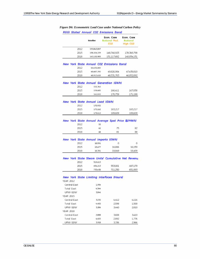
1395BThe New York State Energy Research and Development Authority 91BAppendix D – Energy Market Summaries by Scenario
GE EA&SE 80
Figure D6: Econometric Load Case under National Carbon Policy

1395BThe New York State Energy Research and Development Authority 91BAppendix D – Energy Market Summaries by Scenario
GE EA&SE 81
15.7 WORST CASE UNDER REGIONAL CARBON POLICY
15.7.1 RGGI AND NEW YORK CO2 EMISSIONS
It can be observed that the CO2 emissions in New York are markedly lower in the worst case with regional CO2 allowance costs when compared with the corresponding Base Case20 with high CO2 allowance costs. This is primarily due to the fact the peak load and energy forecast for New York State is much lower in the worst case (same load assumptions are the 15x15 EEPS case) when compared with the Base Case. Also, the gas price is lower when compared to the Base Case, resulting in lower operation of less clean coal and oil-fired generation. For the study year 2012, total CO2 emissions in New York State adds up to nearly 39 million tons with the high CO2 allowance cost assumption in the worst case. For the same year, total CO2 emissions in New York State are nearly 45 million tons with high CO2 allowance cost in the Base Case.
The difference between the worst case and the Base Case is more pronounced in the out years. For the study year 2018, total CO2 emissions in New York State adds up to nearly 30 million tons with the high CO2 allowance cost assumption in the worst case. For the same year, total CO2 emissions in New York State are nearly 38 million tons respectively with the high CO2 allowance cost in the Base Case.
RGGI state CO2 emissions as a whole are also lower in the worst case when compared to the Base Case, primarily driven by the reduction in New York State CO2 emissions.
15.7.2 NYISO ANNUAL SUMMARY
Consistent with the CO2 emissions in New York State, the annual generation also is lower in the worst EEPS case when compared to the Base Case. For the study year 2018, total generation in New York State is approximately 143 thousand GWh with the high CO2 allowance cost assumptions in the worst case. This compares to a total generation in New York State of approximately 153 thousand GWh with the high CO2 allowance cost assumptions in the Base Case.
For the 2018 study year, energy imports in New York State are approximately 20 thousand GWh with the high CO2 allowance cost assumption in the worst case. For the same study year, energy imports in New York State are approximately 27 thousand GWh with the high CO2 allowance cost assumption in the Base Case. As before, it can be seen that NY energy imports in the worst case are lower when compared to the Base Case due to lower demand and higher generation from gas-fired units in New York.
Energy prices in the worst case are much lower than in the Base Case due to lower load and lower marginal prices as a result of lower gas prices. For the 2018 study year, average energy price in New York State is approximately 67 $/MWh with the high CO2 allowance costs assumption in the worst case. For the same study year, average energy price in New York State is approximately 83 $/MWh with the high CO2 allowance costs assumption in the Base Case.
20 Base Case in this report refers to the Base Case with Regional CO2 prices.

1395BThe New York State Energy Research and Development Authority 91BAppendix D – Energy Market Summaries by Scenario
GE EA&SE 82
15.7.3 NYISO ZONAL ANNUAL SUMMARY
In comparison to the Base Case (Regional CO2) results, there is a large decrease in in-state generation in this case primarily due to lower demand. Most of the decrease in generation is evenly distributed in upstate and downstate New York. As observed in the Base Case results, there is congestion on the Central East and Total East interfaces. These two interfaces track flow of energy from western New York to eastern New York. Also, the UPNY-SENY interface, which tracks the flow from upstate to downstate, is also more congested in 2012 when compared with historical congestion. Nevertheless, the congestion on the UPNY-SENY interface is not as severe as in the Base Case due to the reduced transmissions flows as a result of lower demand. Due to these congested interfaces, there is a bigger price separation between upstate and downstate zones. In particular, there is a large price separation between zones A through E and zones F through K due to congestion on the Total East interface. In addition, there is a large price separation between zones E and F due to the congestion on Central East Interface. Still, the price separation between zones F and G due to congestion on the UPNY-SENY interface is not as pronounced as in the Base Case due to the reasons mentioned before.
15.7.4 NYISO UNIT ANNUAL SUMMARY
The results show that the cumulative net revenue of New York Steam units is lower when compared with the Base Case with Regional CO2 prices. This is because the steam units’ capacity factor is lower in the 15x15 case due to the reduced demand and lower gas price. The cumulative net revenue for steam units is approximately $229 million with the high CO2 allowance costs assumption in the worst case for the year 2018. This compared to cumulative net revenue for steam units of approximately $411 million with the high CO2 allowance costs assumption in the Base Case.
On the other hand, the 2018 cumulative net revenues for combined cycle units are approximately $335 million with the high CO2 allowance costs assumption in the worst case. For the Base Case (Regional CO2), the 2018 cumulative net revenues for combined cycle units are approximately $466 million for the high CO2 allowance costs case. The combined cycle units’ revenue is high in the worst case in spite of the lower demand due to lower gas prices.
15.7.5 NYISO CONGESTION SUMMARY
As observed in the Base Case with Regional CO2 prices, there is an increase in congestion on Central East, Total East, and UPNY-SENY interfaces due to increased west to east to south flows. Nevertheless, the congestion on the UPNY-SENY interface is not as severe as the Base Case for the reasons mentioned before. The increase in flows is primarily due to increased generation in upstate NY due to Besicorp Empire generation and higher renewable generation in zones A through E. A comparison of the results for the study years 2012, 2015, and 2018 for the low, medium, or high CO2 allowance cost cases shows the following:
Increasing west to east flows from 2012 to 2018 due to increased renewable generation in zones A through E
Increasing north to south flows from 2012 to 2108 primarily due to increased generation in upstate NY due to Besicorp Empire generation and higher renewable generation in zones A through E

1395BThe New York State Energy Research and Development Authority 91BAppendix D – Energy Market Summaries by Scenario
GE EA&SE 83
Decreasing flow into Long Island from NY due to Neptune HVDC and Caithness CC in the near-term and more expensive units operating in Long Island in the long-term
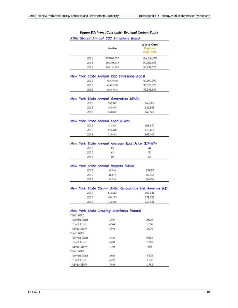
1395BThe New York State Energy Research and Development Authority 91BAppendix D – Energy Market Summaries by Scenario
GE EA&SE 84
Figure D7: Worst Case under Regional Carbon Policy

1395BThe New York State Energy Research and Development Authority 91BAppendix D – Energy Market Summaries by Scenario
GE EA&SE 85
15.8 WORST CASE UNDER NATIONAL CARBON POLICY
15.8.1 RGGI AND NEW YORK CO2 EMISSIONS
It can be observed that the CO2 emissions in the New York are markedly lower in the worst case with National CO2 allowance costs when compared with the corresponding Base Case with high CO2 allowance costs. This is primarily due to the fact the peak load and energy forecast for New York State is much lower in the worst case (same load assumptions are the 15x15 EEPS case) when compared with the Base Case. Also, the gas price is lower when compared to the Base Case resulting in lower operation of less clean coal and oil-fired generation. For the study year 2015, total CO2 emissions in New York State add up to about 36 million tons with the high CO2 allowance cost assumption in the worst case. For the same year, total CO2 emissions in New York State are nearly 45 million tons with high CO2 allowance cost in the Base Case.
The difference between the worst case and the Base Case with National CO2 stays consistent for the length of the study period. For the study year 2018, total CO2 emissions in New York State adds up to approximately 36 million tons with the high CO2 allowance cost assumption in the worst case. For the same year, total CO2 emissions in New York State are nearly 44 million tons respectively with the high CO2 allowance cost in the National Co2 Base Case.
RGGI state CO2 emissions as a whole are also lower in the worst case when compared to the Base Case, largely driven by the reduction in New York State CO2 emissions.
15.8.2 NYISO ANNUAL SUMMARY
Consistent with the CO2 emissions in New York State, the annual generation also is lower in the worst EEPS case with National CO2 when compared to the corresponding Base Case. For the study year 2018, total generation in New York State is approximately 154 thousand GWh with the high CO2 allowance cost assumptions in the worst case national. This compares to a total generation in New York State of approximately 161 thousand GWh with the high CO2 allowance cost assumptions in the Base Case National CO2
For the 2018 study year, energy imports in New York State are approximately eight thousand GWh with the high CO2 allowance cost assumption in the worst case. For the same study year, energy imports in New York State are approximately 17 thousand GWh with the high CO2 allowance cost assumption in the Base Case. As before, it can be seen that NY energy imports in the worst case are lower when compared to the Base Case due to lower demand and higher generation from gas-fired units in New York.
Energy prices in the worst case are much lower than in the Base Case due to lower load and lower marginal prices as a result of lower gas prices. For the 2018 study year, average energy price in New York State is approximately 75 $/MWh with the high CO2 allowance costs assumption in the worst case. For the same study year, average energy price in New York State is approximately 89 $/MWh with the high CO2 allowance costs assumption in the Base Case.
1395BThe New York State Energy Research and Development Authority 91BAppendix D – Energy Market Summaries by Scenario
GE EA&SE 86
15.8.3 NYISO ZONAL ANNUAL SUMMARY
In comparison to the Base Case National CO2 results, there is a large decrease in in-state generation in this case primarily due to lower demand. Most of the decrease in generation is evenly distributed in upstate and downstate New York. As observed in the Base Case results, there is congestion on the Central East and Total East interfaces. These two interfaces track flow of energy from Western New York to Eastern New York. Also, the UPNY-SENY interface, which tracks the flow from upstate to downstate, is also more congested in 2012 when compared with historical congestion. Nevertheless, the congestion on the UPNY-SENY interface is not as severe as in the Base Case due to the reduced transmissions flows as a result of lower demand. Due to these congested interfaces, there is a bigger price separation between upstate and downstate zones. In particular, there is a large price separation between zones A through E and zones F through K due to congestion on the Total East interface. In addition, there is a large price separation between zones E and F due to the congestion on Central East Interface. Still, the price separation between zones F and G due to congestion on the UPNY-SENY interface is not as pronounced as in the Base Case due to the reasons mentioned before.
15.8.4 NYISO UNIT ANNUAL SUMMARY
The results show that the cumulative net revenue of New York Steam units is lower when compared with the Base Case with National CO2 prices. This is because the steam units’ capacity factor is lower in the Worst Case National CO2 due to the reduced demand and lower gas price. The cumulative net revenue for steam units is approximately $286 million with the high CO2 allowance costs assumption in the Worst Case National for the year 2018. This compared to cumulative net revenue for steam units of approximately $501 million with the high CO2 allowance costs assumption in the Base Case National CO2
On the other hand, the 2018 cumulative net revenues for combined cycle units are approximately $433 million with the high CO2 allowance costs assumption in the worst case. For the Base Case (Regional CO2), the 2018 cumulative net revenues for combined cycle units are approximately $516 million for the high CO2 allowance costs case. While still lower than the Base Case National due to the lower demand, the combined cycle units’ revenue is relatively high in the Worst Case National in due lower gas prices.
15.8.5 NYISO CONGESTION SUMMARY
As observed in the Base Case with Regional CO2 prices, there is an increase in congestion on Central East, Total East, and UPNY-SENY interfaces due to increased west to east to south flows. Nevertheless, the congestion on the UPNY-SENY interface is not as severe as the Base Case for the reasons mentioned before. The increase in flows is primarily due to increased generation in upstate NY due to Besicorp Empire generation and higher renewable generation in zones A through E. A comparison of the results for the study years 2012, 2015, and 2018 for the low, medium, or high CO2 allowance cost cases shows the following:
Increasing west to east flows from 2012 to 2018 due to increased renewable generation in zones A through E

1395BThe New York State Energy Research and Development Authority 91BAppendix D – Energy Market Summaries by Scenario
GE EA&SE 87
Increasing north to south flows from 2012 to 2108 primarily due increased generation in upstate NY due to Besicorp Empire generation and higher renewable generation in zones A through E
Decreasing flow into Long Island from NY due to Neptune HVDC and Caithness CC in the near-term and more expensive units operating in Long Island in the long-term

1395BThe New York State Energy Research and Development Authority 91BAppendix D – Energy Market Summaries by Scenario
GE EA&SE 88
Figure D8: Worst Case under National Carbon Policy

1395BThe New York State Energy Research and Development Authority 92BAppendix E – NYISO Capacity Market Description
GE EA&SE 89
16 APPENDIX E – NYISO CAPACITY MARKET DESCRIPTION
Additionally, the NYISO determines the Minimum Locational Installed Capacity Requirements (“LCRs”) for New York City and Long Island, which it uses in conjunction with the locational annual peak load forecast to calculate the locational ICAP requirement. Since the NYISO operates an Unforced Capacity (“UCAP”) market, the ICAP requirements are translated into UCAP requirements, using location-wide forced outage rates. The obligations to satisfy the UCAP requirements are allocated to the Load Serving Entities (LSEs) in proportion to their annual peak load in each area.
The New York State Reliability Council (“NYSRC”) determines the Installed Reserve Margin (“IRM”) for NYCA, which is the amount of planning reserves necessary to meet the reliability standards for New York State. The NYISO uses the IRM in conjunction with the annual peak load forecast to calculate the Installed Capacity (“ICAP”) requirement for NYCA.
LSEs can satisfy their UCAP requirements by contracting for capacity bilaterally, by self-scheduling, or by purchasing in the NYISO-run auctions. The NYISO conducts three UCAP auctions: a forward strip auction where capacity is transacted in six-month blocks for the upcoming capability period, a monthly forward auction where capacity is transacted for the remaining months of the capability period, and a monthly spot auction. The two forward markets are voluntary, but all requirements must be satisfied at the conclusion of the spot market immediately prior to each month.
16.1 USE OF DEMAND CURVES IN THE SPOT AUCTION
Demand curves are used to determine the clearing prices and quantities purchased in each location in each spot auction. The demand curves New York City (NYC), Long Island (LI) and New York Control Area (NYCA) are defined by straight lines between three points as shown in Figure 1.1.
A point at the “Net CONE”, i.e., Cost of New Entry ("CONE") less energy and ancillary services revenues (seasonally adjusted), and the minimum requirement (currently at 116.5% of peak load). For NYCA, the price corresponding to this minimum requirement is $9.92/KW-Month for summer 2009 Auction as shown in Figure 1.1
A point at which the value of additional capacity can be presumed to have declined to zero ("Zero Crossing Point"). The Zero Crossing Point for the currently effective NYCA Demand Curve is 112% of the minimum requirement.
A point corresponding to 1.5 times “Net CONE.” For NYCA, the price corresponding to this point is $13.53/KW-Month.

1395BThe New York State Energy Research and Development Authority 92BAppendix E – NYISO Capacity Market Description
GE EA&SE 90
Figure 1.1: Summer 2009 Demand Curves for NYCA, NYC, and LI
Every three years, the NYISO updates the capacity demand curves. The demand curves are set so that the demand curve price equals the levelized cost of a new peaking unit (net of estimated energy and ancillary services revenue) when the quantity of UCAP procured equals the UCAP requirement.
16.2 DETERMINATION OF MARKET CLEARING PRICES IN THE SPOT AUCTION
In the ICAP Spot Market Auction, the NYISO will also construct a supply curve for all Unforced Capacity offered for each Locality which includes all Capacity in that Locality that LSEs or Installed Capacity Suppliers had designated for use to meet their respective LSE Unforced Capacity Obligations through self-supply, as well as all other Capacity in that Locality offered into the ICAP Spot Market Auction. Similarly, the NYISO will construct a supply curve for the total Unforced Capacity offered in the NYCA.

1395BThe New York State Energy Research and Development Authority 92BAppendix E – NYISO Capacity Market Description
GE EA&SE 91
Market Clearing Price
Figure 1.2: Intersection of Supply and Demand Curves for NYCA
The Market-Clearing Price will be determined for the NYCA, and for each Locality. The Market-Clearing Price for the NYCA will be the price at which the supply curve for the total Unforced Capacity intersects the applicable Demand Curve for the total Installed Capacity market, subject to applicable constraints. This is shown in Figure 1.2. The Market-Clearing Price for a Locality will be the price at which the supply curve for that Locality intersects the Demand Curve for that Locality unless the Market- Clearing Price determined for Rest of State is higher in which case the Market-Clearing Price for that Locality will be set at the Market-Clearing Price for Rest of State.
16.3 NEW YORK CITY MARKET POWER MITIGATION
The purpose of market power mitigation measures is to deter efforts to exercise market power in New York City and help ensure that auction outcomes are protected against the influence of market power. Most of the capacity in New York City is owned by the three Divested Generation Owners ("DGOs") that purchased the capacity from ConEd when it was required to divest itself of substantial amounts of its generation in 1998. A pivotal supplier test is used to determine whether any portion of units owned by a supplier are required to satisfy the minimum capacity requirement for NYC regardless of whether the capacity has been sold to another participant or sold in a prior NYISO administered auction. Resources that fail the test are subject to the offer cap.
In advance of each Obligation Procurement Period (one month), the NYISO would calculate the clearing price that would prevail if all qualified capacity in the NYC Locality were sold, and establish that price as the reference level for each mitigated unit. The mitigated supplier will be required to offer the resources into the spot capacity market at or below its reference level. Offers above the reference level would be reset to the reference level.
Additional information regarding New York City market power mitigation can be found in the Compliance Filing of the New York Independent System Operator, Inc. Regarding the New York City ICAP Market Structure.

1395BThe New York State Energy Research and Development Authority 93BAppendix F – Going-forward Cost Determination
GE EA&SE 92
17 APPENDIX F – GOING-FORWARD COST DETERMINATION
Going-Forward Costs are the costs that could be avoided if a unit is “mothballed” rather than being kept in service and used to provide capacity. A FERC filing made by the NYISO titled “Compliance Filing of The New York Independent System Operator, Inc. regarding the New York City ICAP Market Structure”, Docket No. EL07-39-000 contains detailed information on how GFCs are calculated. A description of going-forward costs in Docket Number EL07-39-000 is included below for reference21.
“Going-forward costs do not include site leasing or land ownership costs, or property taxes. When a unit is mothballed, the land and physical facilities are maintained so that the option of returning the unit to service is preserved. Hence, these costs are not avoidable. If a unit were retired instead of mothballed, site leasing or land ownership costs, and property tax costs, would become avoidable. The types and percentages of costs that are avoidable in a retirement scenario would be case specific. For example, land may be leased and the lease terminated, or the land may be owned and sold. Consequently, the amount of avoidable costs could be significantly different from case to case. Potentially, all of these costs, as well as all of the labor for routine operations and maintenance, routine materials and contract services, administrative and general, and insurance costs, could become avoidable in a retirement scenario.”
This filing identifies the costs that could be avoided by not supplying capacity. They include a percentage22 of the following costs:
1. Labor for routine operations and maintenance 2. Routine materials and contract services 3. Administrative and general costs, and 4. Insurance
Table 1 shows the going-forward costs from the FERC Docket by unit class for New York City. Detailed information on how these going-forward costs are derived can be found in the docket. It is to be noted that the docket includes GFC calculation only for New York City units since the subject of this docket was the NYC capacity market structure. Still, this information can be used as the starting point to determine the going-forward costs for units in Long Island (LI) and the Rest of State (ROS).
21 Affidavit of Christopher Ungate in Docket Number EL07-39-000 22 The percentage of cost in each cost category that would be saved by mothballing a unit (the avoidable cost) was estimated using percentages published by PJM. Additional information can be obtained from Docket Number EL07-39-000
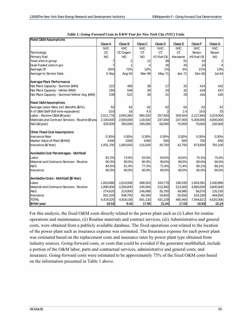
1395BThe New York State Energy Research and Development Authority 93BAppendix F – Going-forward Cost Determination
GE EA&SE 93
Table 1: Going-Forward Costs in $/KW-Year for New York City (NYC) Units Fixed O&M Assumptions
Class A Class B Class C Class D Class E Class F Class G
TechnologyPrimary FuelTotal units in groupDual-Fueled units in groAverage CFAverage In-Service Date
Average Plant PerformanceNet Plant Capacity - Summer (MW)Net Plant Capacity - Winter (MW)Net Plant Capacity - Summer/Winter Avg.
Fixed O&M AssumptionsAverage Labor Rate, incl. Benefits ($/hr)# of O&M Satff (full-time equivalent)Labor - Routine O&M ($/year)Materials and Contract Services - Routine A&G ($/year)
Other Fixed Cost AssumptionsInsurance RateMarket Value of Plant ($/KW)Insurance ($/Year)
Avoidable Cost Percentages - MothballLaborMaterial and Contracts Services - RoutineA&GInsurance
Avoidable Costs - Mothball ($/Year)LaborMaterial and Contracts Services - RoutineA&GInsuranceTOTAL$/KW-year
(MW)
($/yea
NYCCCNG
77
63%5-Sep
222255239
6215.6
2,011,7762,100,000
325,000
0.30%1400
1,001,700
82.2%90.0%84.5%60.0%
1,653,6801,890,000
274,625601,020
4,419,32518.53
NYCCC Cogen
NG21
72%Aug-94
495548522
6216
2,063,3602,500,000
350,000
0.30%1000
1,564,500
73.4%90.0%61.4%60.0%
1,514,5062,250,000
214,900938,700
4,918,1069.43
NYCCTNG
120
12%Mar-99
383939
624.5
580,320118,500190,000
0.30%1000
115,500
63.5%90.0%77.2%60.0%
368,503106,650146,68069,300
691,13317.95
NYCCT
#2 Fuel Oil3916
1%May-71
172421
622
257,920237,00050,000
0.30%500
30,750
63.5%90.0%71.4%60.0%
163,779213,30035,70018,450
431,22921.04
NYCCT
Kerosene5143
3%Jan-71
253229
622.4
309,504237,00070,000
0.30%500
42,750
63.5%90.0%71.4%60.0%
196,535213,30049,98025,650
485,46517.03
NYCSteam
#6 Fuel Oil1010
21%Dec-65
414418416
6216.5
2,127,8405,400,000
70,000
0.30%700
873,600
75.4%90.0%80.1%60.0%
1,604,3914,860,000
56,070524,160
7,044,62116.93
NYCSteam
NG20
13%Jul-64
432437435
6225
3,224,0004,000,000
150,000
0.30%600
782,100
75.4%90.0%80.1%60.0%
2,430,8963,600,000
120,150469,260
6,620,30615.24
For this analysis, the fixed O&M costs directly related to the power plant such as (i) Labor for routine operations and maintenance, (ii) Routine materials and contract services, (iii) Administrative and general costs, were obtained from a publicly available database. The fixed operations cost related to the location of the power plant such as insurance expense was estimated. The Insurance expense for each power plant was estimated based on the replacement costs and insurance rates by power plant type obtained from industry sources. Going-forward costs, or costs that could be avoided if the generator mothballed, include a portion of the O&M labor, parts and contractual services, administrative and general costs, and insurance. Going-forward costs were estimated to be approximately 75% of the fixed O&M costs based on the information presented in Table 1 above.

1395BThe New York State Energy Research and Development Authority 94BAppendix G – Retirement Analysis
GE EA&SE 94
18 APPENDIX G – RETIREMENT ANALYSIS
In order to determine the impact of Green House gas (GHG) policies on the reliability of New York State, it is necessary to identify generators that might mothball or retire if it becomes economically unviable for them to operate. It can be assumed that a generator will continue to operate as a capacity resource as long as it earns enough income to cover all its Fixed Operations and Maintenance costs in addition to covering its variable costs. A generator that is not able to recover all its Fixed O&M costs for multiple years into the future will likely retire. A generator that is not able to recover all its Fixed O&M costs only in the near-term, but is able to do so in the long-term, may choose to operate or mothball in the near-term; the generator will operate as a capacity resource as long as its Net Income is greater than its Going Forward Costs in the near-term. If not, it will mothball.
This appendix discusses how the fixed O&M costs, going-forward costs, and the income for a generator were derived.
18.1 FIXED OPERATIONS AND MAINTENANCE COSTS
Fixed O&M costs are all the costs that are incurred by a power plant regardless of how much energy it produces. Fixed O&M costs are generally divided into the following categories:
Labor for routine operations and maintenance Routine materials and contract services Administrative and general costs Insurance Expense Property Taxes23
The Fixed O&M costs directly related to the power plant such as (i) Labor for routine operations and maintenance, (ii) Routine materials and contract services, (iii) Administrative and general costs, were obtained from the Energy Velocity database24. The fixed operations cost related to the location of the power plant such as insurance expense was estimated. The Insurance expense for each power was estimated based on the replacement costs and insurance rates by power plant type obtained from industry sources.
18.2 GOING-FORWARD COSTS
Going-forward Costs are the costs that could be avoided if a unit is “mothballed” rather than being kept in service and used to provide capacity. Going-forward Costs do not include site leasing or land ownership costs, or property taxes. When a unit is mothballed, the land and physical facilities are maintained so that the option of returning the unit to service is preserved. Hence, these costs are not avoidable.
23 Property taxes are not included in this analysis since the assessment value and the tax rate are determined on a case-by-case basis. Also,property taxes may or may not be avoidable depending on whether the site is owned or leased and whether the plant needs to be decommissioned or not. Still, if it was determined that the property tax would impact the retirement decision for a generator, additional effort was put into estimating the property taxes for that generator.
24 The Energy Velocity database estimates the Fixed O&M costs related to the power plant from a number of sources such as the FERC Form 1 and EIA Form 860.

1395BThe New York State Energy Research and Development Authority 94BAppendix G – Retirement Analysis
GE EA&SE 95
Going-forward costs include a percentage of the following costs:
1. Labor for routine operations and maintenance 2. Routine materials and contract services 3. Administrative and general costs, and 4. Insurance
The going forward costs are estimated to be approximately 75% of the Fixed O&M costs. This is discussed in Appendix G of the report.
18.3 GENERATOR NET INCOME
The Net Income or Cash Flow earned by a generator is calculated as shown in Figure 1.
Figure 1: Net Cash Flow calculation
The net cash flow shown in this figure is the cash flow generated after the principal and interest payments on the debt and the Fixed O&M costs have been paid. Since we are interested in calculating the net revenue (or cash flow) after taxes, but prior to these expenses, we need to make minor modifications to this calculation.
The net after tax income before debt principal and interest payments and Fixed O&M costs can be estimated as follows:
Net Income (After Tax, before debt principal and interest payments and Fixed O&M Costs) = Energy Revenues + Capacity Revenues – Income Taxes
Where, Income Taxes25 = Income Tax Rate*EBITDA
25 The Income Taxes calculated this way would be higher than actual taxes for most units since debt expenses and depreciation (which are not publically available) are deductible from the EBITDA in determining the taxable income. Still, the income tax calculated this way could be assumed to be the maximum tax a generator may have to pay if it is completely depreciated and paid of its debt holders. As a result, the Net Income calculated using this method might be lower than actual Net Income. In the retirement analysis, realizing that the Net Income calculated may be lower than actual income, generators whose Net Income does not cover their Fixed O&M or Going Forward Costs are

1395BThe New York State Energy Research and Development Authority 94BAppendix G – Retirement Analysis
GE EA&SE 96
EBITDA = Energy Revenues26 + Capacity Revenues27 – Fixed O&M costs
checked to see if they will be able to cover those costs if their taxes are lower. If so, the income taxes need to estimate more accurately just for the affected units.
26 Determined in Task 3 of this project
27 Determined in Task 4 of this project

1395BThe New York State Energy Research and Development Authority 95BAppendix H – New York Transfer Limits
GE EA&SE 97
19 APPENDIX H – NEW YORK TRANSFER LIMITS
Source: 2009 NYISO RNA

1395BThe New York State Energy Research and Development Authority 96BAppendix I – NYISO Report on Reliability Impacts
March 18, 2010
20 APPENDIX I – NYISO REPORT ON RELIABILITY IMPACTS
NYSERDA Greenhouse Gas Study: NYISO Reliability Analysis

1395BThe New York State Energy Research and Development Authority 96BAppendix I – NYISO Report on Reliability Impacts
www.nyiso.com NYSERDA Greenhouse Gas Study: NYISO Reliability Analysis | March 18, 2010 | 99
20.1 BACKGROUND
The New York State Energy Research and Development Authority (NYSERDA) is conducting a study to understand and quantify the impact of Greenhouse Gas (GHG) policies on the power grid and obtain the necessary knowledge and justification for proposing measures consistent with the reliability and security of the power grid. In order to determine the impact of GHG policies on the reliability of electricity supply for New York State, it is necessary to identify generators that might mothball or retire if it becomes uneconomical for them to operate. It can be assumed that a generator will continue to operate as a capacity resource as long as it earns enough revenue to cover its Going-Forward Costs (GFC). NYSERDA contracted with General Electric (GE) to perform the study. Using GE’s MAPS program, various system conditions and scenarios based on the State Energy Planning Board study were analyzed. That analysis determined the most likely plant retirements that would occur due to their GFC exceeding their revenues.
The NYSERDA/GE team requested the NYISO to perform a reliability analysis using the GE Multi-Area Reliability Simulation (MARS) program version 2.92. The reliability analysis was conducted to determine if the assumed capacity modifications and retirements would result in the violation of the Loss of Load Expectation (LOLE) criterion of once in 10 years (or 0.1 per year) as established by the Northeast Power Coordinating Council (NPCC) and the New York State Reliability Council (NYSRC). That criterion establishes that the resources available on the electric system in New York should be sufficient such that the probability of an unplanned disconnection of firm load due to resource deficiencies is never greater than once in ten years.
20.2 RELIABILITY ANALYSIS
20.2.1 PROCESS
In order to assess the reliability impact of the capacity retirements/additions resulting from the NYSERDA/GE team’s MAPS study, the NYISO modeled the capacity recommendations provided by the NYSERDA/GE team in MARS and calculated the LOLE. The NYSERDA/GE team developed four base case models (Reference Cases). The first used the load forecast that was used in the NYISO 2009 Reliability Needs Assessment (RNA) base case study. This load forecast is based on achieving approximately 30% of the Energy Efficiency Portfolio Standard (EEPS) and will be referred to as the “NYSERDA GHG RNA” case in this study. This reference case also included approximately 3800MW in additional capacity over the NYISO 2009 RNA base case. The second reference case uses the load forecast based on fully achieving the EEPS and will be referred to as the “NYSERDA GHG 15 x 15” case. Since this case assumes a lower load forecast than the “NYSERDA GHG RNA” case, it also assumes approximately 1,500 MW net less capacity than the “NYSERDA GHG RNA” case. The third reference case assumes a high economic load growth and extreme weather condition and is referred to as the “NYSERDA GHG High Economic Growth” case. This reference case uses the same capacity as the “NYSERDA GHG RNA” case. The fourth reference case assumes an econometric load forecast which does not include any energy efficiency due to the EEPS. This reference case is referred to as the “NYSERDA GHG Econometric” case, The capacity modifications provided by the NYSERDA/GE team for these four reference cases are included as Exhibit B-1 in Appendix BB at the end of this section.

1395BThe New York State Energy Research and Development Authority 96BAppendix I – NYISO Report on Reliability Impacts
www.nyiso.com NYSERDA Greenhouse Gas Study: NYISO Reliability Analysis | March 18, 2010 | 100
As a comparison to the reference cases, four changed cases were also developed by the NYSERDA/GE team. The changed cases include the additional plant retirements due to their GFCs exceeding their revenues as determined by the GE/MAPS analysis.
Four study years (2009, 2012, 2015 and 2018) were evaluated in MARS to determine the NYCA and Zonal LOLEs for each reference and changed case model.
More details regarding the development of the models for the reliability analysis are included in Appendix BB at the end of this section.
The “bubble” diagram and transfer limits used for the NYISO 2009 RNA study are included in Appendix A. The capacity modifications and additional retirement lists provided by the NYSERDA/GE team were reviewed to assess if any of the capacity modifications may have an impact on the system’s transfer limits. The following describes the results of this review:
“NYSERDA GHG RNA” Reference Case
The retirement of 838MW in Zone A were the only retirements listed in the “NYSERDA GHG RNA” reference case capacity modification list that is expected to impact transfer limits. No intra-zonal impacts were considered.
Per the Central East operating nomograms, the Central East and Total East transfer limits are reduced by 75 MW when 838MW in Zone A are unavailable. This reduction was assumed for the retirements.
“NYSERDA GHG 15 x 15” Reference Case
The retirement of 838MW in Zone A and 1200MW in Zone G are the only retirements listed in the “NYSERDA GHG 15 x 15” referenced case capacity modification list that are expected to impact transfer limits. No intra-zonal impacts were considered.
Per the Central East operating nomograms, the Central East and Total East transfer limits are reduced by 75MW when 838MW in Zone A is unavailable. This reduction was assumed for this retirement.
The NYISO 2009 RNA MARS model already includes a dynamic interface rating for the UPNY-Con Ed interface based on the loss of up to 2400MW in Zone G. This nomogram reduces the UPNY- ConEd interface by 300MW for the loss of 600MW and reduces it by an additional 300MW for the loss of 1200MW. For the “NYSERDA GHG 15x15” reference case, this nomogram is expanded to include the loss of up to all 2400MW, with a reduction of the UPNY-Con Ed interface by 300MW per 600MW loss.
“NYSERDA GHG High Economic Growth” Reference Case*

1395BThe New York State Energy Research and Development Authority 96BAppendix I – NYISO Report on Reliability Impacts
www.nyiso.com NYSERDA Greenhouse Gas Study: NYISO Reliability Analysis | March 18, 2010 | 101
The retirement of 838MW in Zone A were the only retirements listed in the “NYSERDA GHG RNA” reference case capacity modification list that is expected to impact transfer limits. No intra-zonal impacts were considered.
Per the Central East operating nomograms, the Central East and Total East transfer limits are reduced by 75 MW when 838MW in Zone A are unavailable. This reduction was assumed for the retirements.
Based on the analysis completed in the NYISO 2009 RNA study for the High Economic Growth and Extreme Weather scenario, the following additional interface transfer limit modifications were included due to the high load growth:
West Central is reduced by 200MW
Central East and Total East are reduced by 75MW (This reduction is in addition to the 75MW reduction due to the retirement of 838MW in Zone A.)
Dunwoodie is reduced by 350MW
“NYSERDA GHG Econometric” Reference Case
Based on the analysis completed in the NYISO 2009 RNA study for the Econometric scenario, the following transfer limit modifications were included due to the load growth:
West Central is reduced by 66MW
Central East and Total East are reduced by 25MW
Dunwoodie is reduced by 116MW.
Changed Cases
For the purposes of the NYSERDA GHG Study, it is assumed that the local TOs would address any voltage impacts due to the plant retirements identified in the “Changed” case lists. Therefore, no analysis was completed to determine the voltage impact of these retirements and no additional modifications to transfer limits were included.
Based on engineering judgment or Local Transmission Plans (LTP), it is anticipated that several of the units listed for the changed cases would result in the need for system upgrades if they were to retire. For example, LIPA has stated in their LTP that the retirement of Far Rockaway Unit 4 would require the construction of five new 501 G power plants over the 20 year study period. Additional units included in the changed case lists which may require system upgrades if they were to retire are noted in Exhibit B-2. No analysis was completed by the NYISO to confirm the need for system upgrades or to determine what upgrades may be required
* This case was provided for reference and was not studied as a part of this analysis.
20.3 RESULTS
Reference Cases
1395BThe New York State Energy Research and Development Authority 96BAppendix I – NYISO Report on Reliability Impacts
www.nyiso.com NYSERDA Greenhouse Gas Study: NYISO Reliability Analysis | March 18, 2010 | 102
No LOLE violations of the 0.1 requirement occurred for all study years for the “NYSERDA GHG RNA” and “NYSERDA GHG 15 x 15” reference cases provided that the assumed load forecast is achieved.
The “NYSERDA GHG High Economic Growth” reference case results in a NYCA LOLE violation at 0.117 in 2009 and increases to 1.042 in 2018.
The “NYSERDA GHG Econometric” reference case results in a NYCA LOLE violation at 0.201 in 2018.
Changed Cases
No LOLE violations of the 0.1 requirement occurred for all study years for the “NYSERDA GHG RNA Load” and “NYSERDA GHG 15 x 15 Load” changed cases provided that the assumed load forecast is achieved. Still, if the 15 x 15 load forecast is not achieved, reliability violations may occur by 2015 for this given capacity condition. Utilizing the capacity assumptions for the “NYSERDA GHG 15 x 15 Case” but only achieving the 30% of the EEPS as assumed in the “NYSERDA GHG RNA Case” results in an NYCA LOLE of 0.214 in 2015 and increases to 0.593 in 2018.
The “NYSERDA GHG High Economic Growth” change case results in a NYCA LOLE violation at 0.117 in 2009 and increases to 1.418 in 2018.
The “NYSERDA GHG Econometric” change case results in a NYCA LOLE violation at 0.18 in 2015 and increases to 0.297 in 2018.
Differences Between NYSERDA GHG and NYISO 2009 RNA
The resulting LOLEs differ from that reported in the NYISO’s 2009 RNA study since different capacity additions and retirements are included in the NYSERDA GHG Study. As noted above, some of the assumed retirements impact the transfer limits which can also impact the LOLE results. The capacity differences are summarized in the Table 1 below by fuel types. More specific details on the capacity differences are included in Appendix BB at the end of this section.

1395BThe New York State Energy Research and Development Authority 96BAppendix I – NYISO Report on Reliability Impacts
www.nyiso.com NYSERDA Greenhouse Gas Study: NYISO Reliability Analysis | March 18, 2010 | 103
Table 1: Capacity Assumption Differences between NYSERDA GHG Reference Cases vs. NYISO 2009
RNA
NYSERDA GHG NYSERDA GHG NYSERDA GHG RNA and Extreme 15 x 15 Case Econometric Economic Growth Capacity as Case Capacity as Case Capacity as Compared to the Compared to the Compared to the NYISO 2009 NYISO 2009 NYISO 2009 RNA RNA Model RNA Model
Model (MW) (MW) (MW) Combined Cycle 1011 504
2080
Coal -53 -76 -53 Combustion Turbine -70 -70 -70 Hydro 180 180 180 Landfill Gas
112 112 552 Nuclear 106 106 106 Oil/Gas -1127 -2148 -347 Wind 3660 3660 3660 3819 2268 6108

1395BThe New York State Energy Research and Development Authority 96BAppendix I – NYISO Report on Reliability Impacts
www.nyiso.com NYSERDA Greenhouse Gas Study: NYISO Reliability Analysis | March 18, 2010 | 104
20.4 SUMMARY
NYISO completed a reliability analysis in order to determine the impact of NYSERDA/GE’s team recommended capacity modifications and additional retirements on the reliability of the system. Table 2 summarizes the LOLE results for the reference and changed cases.
Table 2: Reliability Analysis Summary
LOLE Results NYCA 2018 LOLE Delta
NYSERDA GHG RNA Reference Case No violation Changed Case No violation +0.039 NYSERDA GHG 15 x 15 Reference Case No violation Changed Case No violation if full 15 x 15
EEPS is achieved. A violation by 2015 may occur if only 30% of the EEPS is achieved.
+0.007 +0.592
NYSERDA GHG Extreme Economic Growth Reference Case A NYCA violation at 0.117
occurs in 2009 and increases to 1.042 in 2018.
Changed Case A NYCA violation at 0.117 occurs in 2009 and increases to 1.418 in 2018.
+0.376
NYSERDA GHG Econometric Reference Case A NYCA violation at
occurs in 2018. 0.201
Changed Case A NYCA violation at 0.18 occurs in 2015 and increases to 0.297 in 2018.
+0.096

1395BThe New York State Energy Research and Development Authority 96BAppendix I – NYISO Report on Reliability Impacts
www.nyiso.com NYSERDA Greenhouse Gas Study: NYISO Reliability Analysis | March 18, 2010 | 105
21 APPENDIX AA
D
OntarioOntario
PJM West
CT
Maine
Rest ofNew England
BostonBoston
PJM Mid-Atlantic
New England
DysingerEast
New York Control AreaTransmission System RepresentationFor 2009 RNA StudySummer Ratings
AB
C
E
PJM Central PJM
East
AstW
PJM East-NY East
550
550
550
550
1,550
1,450
1,550
1,450
2,200
1,999
1,3001,770
800
200
4,000
300
200
1,500
2,000
2,0001,500
2,600
1,600
West Central 1,999
4,270
VolneyEast
QuebecQuebec
400
350
1,0001,500
F
G
H
I
J
Moses South
1,600
3,150
1,999
Central East +
Fraser-Gilboa
Marcy South
CE Group3,4004,550
1,700
3,450
1,999
UPNY/SENY: 5,150 MW
Total East1,9996,000
150
0
800
800
600
2,200
1,400
3,600
SWCT
2,350 330
286/200
UPNY/CE
5,000 / 4,700 / 4,400
1,999G-SENY: 6,000 MW
Millwood South
8,450
1,290
530Y49/Y50
1,9994,000
CE-LIPA
Neptune Controllable Line
660
660
LI Sum576/397/223
LI West306*99,999
486/414/342/304/232
175
1,500
1,200 / 800 / 700 / 600
99,999
500
286
NE / NY1,200 to NY1,525 to NE
Cross Sound Controllable Line
Grouping used for monitoring
330KDunwoodie South
0
NYCA zonal connections
Standard Grouping
NYCA zonal interfaces
External connections
A NYCA zone
NYCA internal transfer limits
External transfer limits
A “Dummy” zone for analysis
AG
1,4656,500
200/3099,999
1,999
800
MISO Cedars167
0
VFT

1395BThe New York State Energy Research and Development Authority 96BAppendix I – NYISO Report on Reliability Impacts
www.nyiso.com NYSERDA Greenhouse Gas Study: NYISO Reliability Analysis | March 18, 2010 | 106
22 APPENDIX BB: MARS BASE CASE MODELS
22.1 MODEL ASSUMPTIONS
Study Period
The Reliability Study looks out over a 10 year period from 2009 to 2018. The years studied include 2009, 2012, 2015 and 2018.
Base Model
A base model was created by modifying the 2009 Installed Reserve Margin (IRM) model. Modifications to this one year IRM model are necessary in order to include known changes that will take place over the planning period as determined in the 2009 Reliability Needs Assessment (RNA) Base Case. This base model was used as the starting point for creating the reference cases being evaluated. The following modifications were made to the IRM model base on the NYISO 2009 Reliability Needs Assessment (RNA) Base Case:
The following generation additions and uprates that were included in the Base Case of the 2009 RNA were added:
Empire Generating (Besicorp) 660 MW
Blenheim-Gilboa Unit 1 30 MW
Blenheim-Gilboa Unit 2: 30 MW
Nine Mile Point Unit 2: 168 MW
The following generator retirements that were included in the Base Case of the 2009 RNA were included:
(a) 890.7 MW in ZONE J
The transfer limits used in the NYISO 2009 RNA base case were included.
All external area loads and capacity data were held constant through out the study period.
22.2 LOAD FORECAST
NYSERDA GHG RNA
The “NYSERDA GHG RNA” Case uses the load forecast used in the NYISO 2009 RNA Base Case. This load forecast is based on achieving approximately 30% of the Energy Efficiency Portfolio Standard (EEPS) as shown in Table B-1.
Table B-1: 2009 RNA Base Case Load Forecast (MW) (Per NYISO 2009 RNA Report Table 3-1)

1395BThe New York State Energy Research and Development Authority 96BAppendix I – NYISO Report on Reliability Impacts
www.nyiso.com NYSERDA Greenhouse Gas Study: NYISO Reliability Analysis | March 18, 2010 | 107
2009 2012 2015 2018 2009 RNA Base 34,059 34,586 35,029 35,658 Case
NYSERDA GHG 15 x 15 Case
The “NYSERDA GHG 15 x 15” case uses the load forecast used in Scenario 2 of the NYISO 2009 RNA. This load forecast is based on achieving 100% of the EEPS as shown in Table B-2.
Table B-2: 2009 RNA Scenario 2 Load Forecast (MW) (Per NYISO 2009 RNA Report Table 3-1) 2009 2012 2015 2018 2009 RNA 33,704 32,722 31,227 32,209 Scenario 2
NYSERDA GHG High Economic Growth Case
The “NYSERDA GHG High Economic Growth” case uses the load forecast used in the High Load Growth and Extreme Weather scenario of the NYISO 2009 RNA. This load forecast is based a high load forecast (95th percentile) and extreme weather conditions (high summer temperatures consistent with the 95th percentile of historic weather conditions) as shown in Table B-3.
Table B-3: 2009 RNA High Load Growth and Extreme Weather Load Forecast (MW) (Per NYISO 2009 RNA
Report Table 4-14)
2009 2012 2015 2018 2009 RNA High 36,607 37,211 37,737 38,464 Growth
NYSERDA GHG Econometric Case*
The “NYSERDA GHG Econometric” case uses the load forecast from the Econometric Load Forecast scenario of the NYISO 2009 RNA as shown in Table B-4. This forecast did not include any energy efficiency penetration levels associated with the EEPS proposal.
Table B-4: 2009 RNA Econometric Load Forecast (MW)
(Per NYISO 2009 RNA Report Table 4-9) 2009 2012 2015 2018 2009 RNA 34,247 35,452 36,708 37,784 Econometric
* THIS CASE WAS PROVIDED FOR REFERENCE AND WAS NOT STUDIED AS A PART OF THIS ANALYSIS.

1395BThe New York State Energy Research and Development Authority 96BAppendix I – NYISO Report on Reliability Impacts
www.nyiso.com NYSERDA Greenhouse Gas Study: NYISO Reliability Analysis | March 18, 2010 | 108
MARS RESULTS
22.2.1 NYSERDA GHG RNA CASE
Reference Case
Table B-5 provides the LOLE results for the “NYSERDA GHG RNA” reference case. The resultant LOLE criterion of 0.1 per year is not violated for any area for any study year.
Table B-5: NYSERDA GHG RNA Reference Case LOLE
Zone
NYSERDA GHG RNA Reference Case 2009 2012 2015 2018
A 0.0 0.0 0.0 0.0 B 0.0 0.0 0.001 0.004 C 0.0 0.0 0.0 0.0 D 0.0 0.0 0.0 0.0 E 0.0 0.0 0.0 0.001 F 0.0 0.0 0.0 0.0 G 0.0 0.0 0.0 0.001 H 0.0 0.0 0.0 0.0 I 0.001 0.002 0.006 0.025 J 0.001 0.002 0.007 0.027 K 0.0 0.0 0.0 0.0 NYCA 0.001 0.003 0.007 0.029

1395BThe New York State Energy Research and Development Authority 96BAppendix I – NYISO Report on Reliability Impacts
www.nyiso.com NYSERDA Greenhouse Gas Study: NYISO Reliability Analysis | March 18, 2010 | 109
Changed Case
Table B-6 provides the LOLE for the “NYSERDA GHG RNA” changed case. The additional retirements included in this case increases the LOLE in 2018 by .039. Still, the LOLE criterion of 0.1 per year is not violated for any area for any study year.
Table B-6: NYSERDA GHG RNA Changed Case LOLE
Zone
NYSERDA GHG RNA Changed Case 2009 2012 2015 2018
A 0.0 0.0 0.0 0.0 B 0.0 0.0 0.003 0.011 C 0.0 0.0 0.0 0.0 D 0.0 0.0 0.0 0.0 E 0.0 0.0 0.001 0.004 F 0.0 0.0 0.0 0.0 G 0.0 0.0 0.001 0.003 H 0.0 0.0 0.000 0.000 I 0.001 0.004 0.018 0.060 J 0.001 0.004 0.019 0.061 K 0.0 0.0 0.001 0.002 NYCA 0.001 0.005 0.021 0.068

1395BThe New York State Energy Research and Development Authority 96BAppendix I – NYISO Report on Reliability Impacts
www.nyiso.com NYSERDA Greenhouse Gas Study: NYISO Reliability Analysis | March 18, 2010 | 110
22.2.2 NYSERDA GHG 15 X 15 CASE
Reference Case
Table B-7 provides the LOLE results for the base “NYSERDA GHG 15 x 15” reference case. Even though there is less capacity assumed for this case, the lower load forecast is sufficient enough such that the LOLE is not violated through out the study period.
Table B-7: NYSERDA GHG 15 x 15 Reference Case LOLE
Zone
NYSERDA GHG 15 x 15 Reference Case 2009 2012 2015 2018
A 0.0 0.0 0.0 0.0 B 0.0 0.0 0.0 0.0 C 0.0 0.0 0.0 0.0 D 0.0 0.0 0.0 0.0 E 0.0 0.0 0.0 0.0 F 0.0 0.0 0.0 0.0 G 0.0 0.001 0.0 0.0 H 0.0 0.0 0.0 0.0 I 0.0 0.005 0.0 0.001 J 0.0 0.004 0.0 0.001 K 0.0 0.0 0.0 0.0 NYCA 0.001 0.005 0.0 0.001

1395BThe New York State Energy Research and Development Authority 96BAppendix I – NYISO Report on Reliability Impacts
www.nyiso.com NYSERDA Greenhouse Gas Study: NYISO Reliability Analysis | March 18, 2010 | 111
Changed Case
Table B-8 provides the LOLE for the “NYSERDA GHG 15 x 15” changed case. The additional retirements included in this case increases the NYCA LOLE in 2018 by .007. Still, the LOLE criterion of 0.1 per year is not violated for any area for any study year.
Neverthelesss, if the 15 x 15 load forecast is not achieved, reliability violations may occur by 2015 for this given capacity condition. Table B-9 shows the results based on using the capacity assumptions for the “NYSERDA GHG 15 x 15 Case” but only achieving the 30% of the EEPS as assumed in the “NYSERDA GHG RNA Case”. This shows that the NYCA LOLE would exceed 0.1 by 2015 and would approach 0.6 by 2018. The primary differences impacting these LOLE results are that the “NYSERDA GHG 15 x 15 Case” has over 1500MW less in fossil fuel capacity than the “NYSERDA GHG RNA Case”. This will result in a much lower reliable system if the loads aren’t sufficiently reduced to offset this lack of generation capacity.
Table B-8: NYSERDA GHG 15 x 15 Changed Case LOLE
Zone
NYSERDA GHG 15 x 15 Changed Case 2009 2012 2015 2018
A 0.0 0.0 0.0 0.000 B 0.0 0.0 0.0 0.001 C 0.0 0.0 0.0 0.0 D 0.0 0.0 0.0 0.0 E 0.0 0.0 0.0 0.0 F 0.0 0.0 0.0 0.0 G 0.0 0.002 0.0 0.002 H 0.0 0.0 0.0 0.0 I 0.0 0.009 0.0 0.007 J 0.0 0.007 0.0 0.006 K 0.0 0.000 0.0 0.000 NYCA 0.001 0.01 0.0 0.008

1395BThe New York State Energy Research and Development Authority 96BAppendix I – NYISO Report on Reliability Impacts
www.nyiso.com NYSERDA Greenhouse Gas Study: NYISO Reliability Analysis | March 18, 2010 | 112
Table B-9: NYSERDA GHG 15 x 15 Changed Case w/ 30% EEPS Load Forecast
LOLE
Zone
NYSERDA GHG 15 x 15 Changed Case w/ 30% EEPS Load Forecast 2009 2012 2015 2018
A 0.0 0.0 0.000 0.000 B 0.0 0.0 0.009 0.025 C 0.0 0.0 0.000 0.0 D 0.0 0.0 0.000 0.0 E 0.0 0.0 0.003 0.0 F 0.0 0.0 0.000 0.0 G 0.0 0.029 0.061 0.185 H 0.0 0.0 0.001 0.0 I 0.0 0.089 0.199 0.555 J 0.0 0.074 0.170 0.498 K 0.0 0.001 0.001 0.002 NYCA 0.001 0.096 0.214 0.593

1395BThe New York State Energy Research and Development Authority 96BAppendix I – NYISO Report on Reliability Impacts
www.nyiso.com NYSERDA Greenhouse Gas Study: NYISO Reliability Analysis | March 18, 2010 | 113
22.3 NYSERDA GHG HIGH ECONOMIC GROWTH
Reference Case
Table B-10 provides the LOLE for the “NYSERDA GHG High Economic Growth” reference case. The high load forecast included in this case results in a NYCA LOLE at 0.117 in 2009 and increasing to 1.042 in 2018 thus violating the 0.1 criterion for all study years. Also the LOLE for Zones I and J exceed 0.1 in 2012.
Table B-10: NYSERDA GHG High Economic Growth Case LOLE
NYSERDA GHG High Economic Growth Reference Case
Zone 2009 2012 2015 2018 A 0.0 0.0 0.0 0.0 B 0.039 0.062 0.074 0.132 C 0.0 0.0 0.0 0.0 D 0.0 0.0 0.0 0.0 E 0.014 0.027 0.037 0.079 F 0.0 0.0 0.0 0.0 G 0.003 0.007 0.011 0.026 H 0.001 0.001 0.001 0.002 I 0.086 0.226 0.415 0.884 J 0.098 0.239 0.457 0.999 K 0.035 0.019 0.020 0.037 NYCA 0.117 0.257 0.481 1.042

1395BThe New York State Energy Research and Development Authority 96BAppendix I – NYISO Report on Reliability Impacts
www.nyiso.com NYSERDA Greenhouse Gas Study: NYISO Reliability Analysis | March 18, 2010 | 114
Changed Case
Table B-11 provides the LOLE for the “NYSERDA GHG High Economic Growth” changed case. The additional retirements included in this case increases the NYCA LOLE in 2018 by 0.376. It also causes an LOLE violation in Zone K in 2018.
Table B-11: NYSERDA GHG High Economic Growth Changed Case LOLE
NYSERDA GHG High Economic Growth Changed Case
Zone 2009 2012 2015 2018 A 0.000 0.000 0.000 0.000 B 0.039 0.062 0.112 0.183 C 0.000 0.000 0.000 0.000 D 0.000 0.000 0.000 0.000 E 0.014 0.027 0.064 0.111 F 0.000 0.000 0.000 0.000 G 0.003 0.007 0.031 0.061 H 0.001 0.001 0.002 0.002 I 0.086 0.226 0.635 1.263 J 0.098 0.239 0.674 1.362 K 0.035 0.019 0.074 0.122 NYCA 0.117 0.257 0.709 1.418

1395BThe New York State Energy Research and Development Authority 96BAppendix I – NYISO Report on Reliability Impacts
www.nyiso.com NYSERDA Greenhouse Gas Study: NYISO Reliability Analysis | March 18, 2010 | 115
22.4 NYSERDA GHG ECONOMETRIC
Reference Case
Table B-12 provides the LOLE for the “NYSERDA Econometric” reference case. The load forecast included in this case results in a NYCA LOLE violation at 0.201 in 2018.Also the LOLE for Zones I and J exceed 0.1 in 2018.
Table B-12: NYSERDA GHG Econometric Case LOLE NYSERDA GHG Econometric Reference Case Zone 2009 2012 2015 2018 A 0.0 0.0 0.0 0.0 B 0.001 0.001 0.007 0.006 C 0.0 0.0 0.0 0.0 D 0.0 0.0 0.0 0.0 E 0.000 0.000 0.002 0.002 F 0.0 0.0 0.0 0.0 G 0.000 0.000 0.002 0.002 H 0.000 0.000 0.001 0.001 I 0.001 0.013 0.087 0.142 J 0.001 0.013 0.091 0.192 K 0.000 0.000 0.002 0.001 NYCA 0.002 0.015 0.099 0.201

1395BThe New York State Energy Research and Development Authority 96BAppendix I – NYISO Report on Reliability Impacts
www.nyiso.com NYSERDA Greenhouse Gas Study: NYISO Reliability Analysis | March 18, 2010 | 116
Changed Case
Table B-13 provides the LOLE for the “NYSERDA GHG Econometric” changed case. The additional retirements included in this case caused a NYCA LOLE violation of 0.18 in 2015 that increases to 0.297 in 2018. The NYCA LOLE in 2018 is an increase of 0.096 over the reference case. The changed case also results in the LOLE exceeding 0.1 for Zones I and J in 2015 and 2018.
Table B-13: NYSERDA GHG Econometric Changed Case LOLE
NYSERDA GHG Econometric Changed Case
Zone 2009 2012 2015 2018 A 0.000 0.000 0.000 0.000 B 0.001 0.001 0.016 0.016 C 0.000 0.000 0.000 0.000 D 0.000 0.000 0.000 0.000 E 0.000 0.000 0.005 0.005 F 0.000 0.000 0.000 0.000 G 0.000 0.000 0.007 0.006 H 0.000 0.000 0.001 0.001 I 0.001 0.013 0.160 0.238 J 0.001 0.013 0.167 0.281 K 0.000 0.000 0.010 0.004 NYCA 0.002 0.015 0.180 0.297
22.5 SUMMARY
The capacity modifications for the reference cases and the additional retirements for the changed cases for the “NYSERDA GHG RNA” and “NYSERDA GHG 15 x 15” cases did not result in any LOLE violations of once in 10 years throughout the study period provided that the corresponding load forecast is achieved. Still, if the full energy portfolio standard load forecast is not achieved, then a violation may occur in the “NYSERDA GHG 15 x 15” changed case starting in year 2015.
The capacity modifications for the reference cases and the additional retirements for the changed cases for the “NYSERDA GHG High Economic Growth” cases resulted in a NYCA LOLE violation of once in 10 years throughout the study period and an LOLE violation in Zones I and J starting in 2012 and in Zone K starting in 2018.
The capacity modifications for the reference cases for the “NYSERDA GHG Econometric” case resulted in a NYCA, Zone I and J LOLE violations of once in 10 years for year 2018. The changed case resulted in advancing the LOLE violations to 2015.