the new (g – 2) experiment: a proposal to measure the muon ... · test of lorentz and cpt...
TRANSCRIPT

The New (g – 2) Experiment:
A Proposal to Measure the Muon Anomalous
Magnetic Moment to ±0.14 ppm Precision
Submitted to FNAL
February 9, 2009
New (g – 2) Collaboration

The New (g − 2) Experiment:
A Proposal to Measure the Muon Anomalous Magnetic Moment
to ±0.14 ppm Precision
New (g − 2) Collaboration: R.M. Carey1, K.R. Lynch1, J.P. Miller1,
B.L. Roberts1, W.M. Morse2, Y.K. Semertzidis2, V.P. Druzhinin3, B.I. Khazin3,
I.A. Koop3, I. Logashenko3, S.I. Redin3, Y.M. Shatunov3, Y. Orlov4, R.M. Talman4,
B. Casey5, J. Johnstone5, D. Harding5, A. Klebaner5, A. Leveling5, J-F. Ostiguy5,
N. Mokhov5, D. Neuffer5, M. Popovic5, S. Strigonov5, M. Syphers5, G. Velev5,
S. Werkema5, F. Happacher6, G. Venanzoni6, P. Debevec7, M. Grosse-Perdekamp7,
D.W. Hertzog7, P. Kammel7, C. Polly7, K.L. Giovanetti8, K. Jungmann9,
C.J.G. Onderwater9, N. Saito10, C. Crawford11, R. Fatemi11, T.P. Gorringe11,
W. Korsch11, B. Plaster11, V. Tishchenko11, D. Kawall12, T. Chupp13,
C. Ankenbrandt14, M.A Cummings14, R.P. Johnson14, C. Yoshikawa14, Andre
de Gouvea15, T. Itahashi16, Y. Kuno16, G.D. Alkhazov17, V.L. Golovtsov17,
P.V. Neustroev17, L.N. Uvarov17, A.A. Vasilyev17, A.A. Vorobyov17, M.B. Zhalov17,
F. Gray18, D. Stockinger19, S. Baeßler20, M. Bychkov20, E. Frlez20, and D. Pocanic20
1Department of Physics, Boston University, Boston, MA 02215, USA
2Brookhaven National Laboratory, Upton, NY 11973, USA
3Budker Institute of Nuclear Physics, 630090 Novosibirsk, Russia
4Newman Laboratory, Cornell University, Ithaca, NY 14853, USA
5Fermi National Accelerator Laboratory, Batavia, IL 60510, USA
6Laboratori Nazionali di Frascati, INFN, I-00044 Frascati (Rome), Italy
7Department of Physics, University of Illinois, Urbana-Champaign, IL 61801, USA
8Department of Physics, James Madison University, Harrisonburg, VA 22807, USA
9Kernfysisch Versneller Instituut, Rijksuniversiteit,
Groningen, NL 9747 AA Groningen, The Netherlands
10KEK, High Energy Accelerator Research Organization, Tsukuba, Ibaraki 305-0801, Japan
11Department of Physics, University of Kentucky, Lexington, Ky 40506, USA
1

12Department of Physics, University of Massachusetts, Amherst, MA 01003, USA
13Physics Department, University of Michigan, Ann Arbor, MI 48109, USA
14Muons, Inc., Batavia, IL 60510, USA
15Physics & Astronomy Department, Northwestern University, Evanston, IL 60208, USA
16Department of Physics, Osaka University, Toyonaka, Osaka 560-0043, Japan
17Petersburg Nuclear Physics Institute, Gatchina 188350, Russia
18Department of Physics and Computational
Science, Regis University, Denver, CO 80221, USA
19Technische Universitat Dresden, Institut fur Kern-
und Teilchenphysik, D-01062 Dresden, Germany
20Department of Physics, The University of Virginia, Charlottesville, VA 22904, USA
Request: 4 × 10²⁰ protons on target in 6 of
20 Booster batches during 15 Hz operation
February 9, 2009
Contactpersons: David W. Hertzog ([email protected], 217-333-3988)
B. Lee Roberts ([email protected], 617-353-2187)
2
Abstract
We propose to measure the muon anomalous magnetic moment, aµ , to 0.14 ppm—a fourfold
improvement over the 0.54 ppm precision obtained in the BNL experiment E821. The muon
anomaly is a fundamental quantity and its precise determination will have lasting value. The
current measurement was statistics limited, suggesting that greater precision can be obtained in a
higher-rate, next-generation experiment. We outline a plan to use the unique FNAL complex of
proton accelerators and rings to produce high-intensity bunches of muons, which will be directed
into the relocated BNL muon storage ring. The physics goal of our experiment is a precision on the
muon anomaly of 16×10−11, which will require 21 times the statistics of the BNL measurement, as
well a factor of 3 reduction in the overall systematic error. Our goal is well matched to anticipated
advances in the worldwide effort to determine the standard model (SM) value of the anomaly. The
present comparison, ∆aµ(Expt.− SM) = (295 ± 81) × 10−11, is already suggestive of possible new
physics contributions to the muon anomaly. Assuming that the current theory error of 51× 10−11
is reduced to 30 × 10−11 on the time scale of the completion of our experiment, a future ∆aµ
comparison would have a combined uncertainty of ≈ 34 × 10−11, which will be a sensitive and
complementary benchmark for proposed standard model extensions. The experimental data will
also be used to improve the muon EDM limit by up to a factor of 100 and make a higher-precision
test of Lorentz and CPT violation.
We describe in this Proposal why the FNAL complex provides a uniquely ideal facility for a
next-generation (g − 2) experiment. The experiment is compatible with the fixed-target neutrino
program; indeed, it requires only the unused Booster batch cycles and can acquire the desired
statistics in less than two years of running. The proton beam preparations are largely aligned with
the new Mu2e experimental requirements. The (g − 2) experiment itself is based on the solid
foundation of E821 at BNL, with modest improvements related to systematic error control. We
outline the motivation, conceptual plans, and details of the tasks, anticipated budget, and timeline
in this proposal.
3

Contents
I. Executive Summary 7
II. Introduction 9
A. Principle of the Experiment 11
B. Experimental Specifics 14
III. The Physics Case for a New (g − 2) Experiment 16
A. The Standard-Model Value of aµ 18
1. QED and Weak Contributions 18
2. The Hadronic Contribution 19
3. The Lowest-order Hadronic Contribution 21
4. BaBar e+e− → π+π− Data 23
5. ahad;LOµ from Hadronic τ decay 23
6. The Hadronic Light-by-Light Contribution 24
B. Summary of the Standard Model Value and Comparison with Experiment 24
1. R(s) Measurements and the Higgs Mass, MH 26
C. Expected Improvements in the Standard Model Value 27
D. Physics Beyond the Standard Model 28
1. aµ as a benchmark for models of new physics 31
2. aµ is sensitive to quantities that are difficult to measure at the LHC 33
IV. A New (g − 2) Experiment 37
A. Scientific Goal 37
B. Key Elements to a New Experiment 37
C. The Expected Flash at FNAL 39
D. Event Rate and POT Request Calculation 40
V. Beam Preparation 43
A. Meeting the Experimental Requirements 44
B. Bunch Formation 46
C. Beam Delivery and Transfer 48
D. Target Station, Pion Capture and Decay 50
4
E. Toward a Beam Rate Calculation 50
F. Experimental Facility 51
G. Environmental Assessment 52
H. Opening the Inflector Ends 53
I. Accelerator R&D 53
J. Muon Storage Ring Magnet 55
K. Relocating the Storage Ring to FNAL 56
VI. The Precision Magnetic Field 59
A. Methods and Techniques 59
B. Past improvements 61
C. Shimming the Storage Ring Magnetic Field 63
D. Further Improvements 66
VII. ωa Measurement 69
A. Overview 69
B. Electromagnetic Calorimeters 73
C. Position-Sensitive Detectors 74
D. Waveform Digitizers for Calorimeter Readout 75
E. Clock systems 78
F. Data Acquisition 79
VIII. Systematic uncertainties on ωa 81
A. Gain Changes and Energy-Scale Stability 82
B. Lost Muons 83
C. Pileup 84
D. Coherent Betatron Oscillations 86
E. Electric Field and Pitch Correction 87
F. ωa Systematic Uncertainty Summary 88
IX. Parasitic Measurement of the Muon Electric Dipole Moment 88
A. E821 Traceback System 90
B. Improved Traceback System 91
5

X. Manpower, Cost Estimate and Schedule 93
A. Manpower 93
B. Cost Estimate 93
C. Schedule 97
XI. Planned R&D Efforts 98
XII. Summary of the Request 100
References 101
A. Muon Collection and Transport Beamline 106
1. Beamline Overview 106
2. Pion production 108
3. Transport in AP2 109
4. Performance Estimate 110
B. Beam Dynamics and Scraping 112
1. The Kicker and Quadrupoles 112
2. Beam Dynamics in the Ring 112
3. Oscillating Dipole Method of Scraping 115
4. Pulsed Octupole Method to Remove the CBO 117
C. New Calorimeters 121
6

I. EXECUTIVE SUMMARY
The muon anomalous magnetic moment aµ is a low-energy observable, which can be both
measured and computed to high precision. The comparison between experiment and the
standard model (SM) is a sensitive test of new physics. At present, both measurement and
theory cite similar sub-ppm uncertainties, and the “(g− 2) test” is being used to constrain
standard model extensions. Indeed, the difference, ∆aµ(Expt− SM) = (295 ± 81) × 10−11,
is a highly cited result, and a possible harbinger of new TeV-scale physics. The present
proposal is to reduce the experimental uncertainty to create a more precise (g − 2) test
that will sharply discriminate among models. A significant effort is ongoing worldwide to
reduce the uncertainty on the SM contributions. During the time required to mount, run
and analyze the New (g − 2) Experiment, we expect that the theory uncertainty will have
improved considerably.
The experimental determination of the muon anomalous magnetic moment aµ has an
uncertainty of 0.54 ppm, which is dominated by the statistical error of 0.46 ppm. This
suggests that a further increase in precision is possible if a higher integrated number of
stored muons can be obtained. We propose to measure aµ at FNAL to an uncertainty of
0.14 ppm, derived from a 0.10 ppm statistical sample and roughly equal 0.07 ppm systematic
uncertainty contributions from measurement of the magnetic field and from measurement
of the precession frequency. Twenty-one times more events are required compared to the
E821 experiment, which completed its data taking in 2001. Our proposal efficiently uses the
FNAL beam complex—in parasitic mode to the high-energy neutrino program—to produce
the necessary flux of muons, which will be injected and stored in the relocated muon storage
ring. In less than two years of running, the statistical goal can be achieved for positive
muons. A follow-up run using negative muons is possible, depending on future scientific
motivation. Two additional physics results will be obtained from the same data: a new
limit on the muon’s electric dipole moment; and, a more stringent limit on possible CPT or
Lorentz violation in muon spin precession.
The beam concept at FNAL can deliver the required flux at a higher injection frequency
compared to BNL. With the long FNAL decay channel, the stored muon rate per proton
rises considerably, while largely eliminating the troubling hadronic-induced beam-injection
background that plagued the BNL measurement. The new experiment will require upgrades
7

and maintenance on several components of the storage ring and a new suite of segmented
electromagnetic calorimeters and position-sensitive detectors. A modern data acquisition
system will be used to read out waveform digitizer data and store it so that both the
traditional event mode and a new integrating mode of data analysis can both be used in
parallel. Improvements in the field-measuring system are also required. They will both follow
well-developed upgrade plans and address challenges for even further precision through a
program of R&D efforts.
A challenging aspect of the new experiment will be the disassembly, transport, and re-
assembly of the BNL storage ring (See Fig. 1). We have examined the tasks in consultation
with the lead project engineers and can estimate the time and cost required with a fair
degree of confidence. The ring will be placed in a new and relatively modest building at
FNAL at the end of the AP2 line (near the AP0 blockhouse). The critical timescale to
be ready for data taking is driven by the effort to relocate the ring to FNAL and to re-
shim it to very high field uniformity. Detector and software development will take place
concurrently. The Laboratory cost for 1) the ring relocation; 2) special beamline elements;
and 3) detector, electronics and DAQ systems, is estimated to be approximately $20 M.
The Collaboration is built from a core group of E821 participants, together with many new
domestic and international groups.
Our planning envisions a development period following scientific approval of approxi-
mately 1 year, during which time we would complete a detailed design and cost document.
During this time period, we will complete the plans to move the storage ring, finalize the
beam optics, site and design the building, and begin R&D on the detectors, electronics,
and field-measuring systems. These tasks mainly involve personnel, and do not incur large
capital costs. We note that many of the beam developments required are also needed for
the approved Mu2e experiment.
8

FIG. 1: The existing muon storage ring that will be relocated to FNAL for the New (g − 2)
Experiment.
II. INTRODUCTION
The muon magnetic moment is related to its intrinsic spin by the gyromagnetic ratio gµ:
~µµ = gµ
(q
2m
)~S, (1)
where gµ = 2 is expected for a structureless, spin-12
particle of mass m and charge q = ±|e|,with radiative corrections (RC), which couple the muon spin to virtual fields, introduce an
anomalous magnetic moment defined by
aµ =1
2(gµ − 2). (2)
The leading RC is the lowest-order (LO) quantum electrodynamic process involving the
exchange of a virtual photon, the “Schwinger term,” [1] giving aµ(QED; LO) = α/2π ≈1.16× 10⁻³. The complete standard model value of aµ , currently evaluated to a precision of
approximately 0.5 ppm (parts per million), includes this first-order term along with higher-
order QED processes, electroweak loops, hadronic vacuum polarization, and other higher-
order hadronic loops. The measurement of aµ in Brookhaven E821 was carried out to a
similar precision [2]. The difference between experimental and theoretical values for aµ is a
9

valuable test of the completeness of the standard model. At sub-ppm precision, such a test
explores TeV-scale physics. The present difference between experiment and theory is
∆aµ(Expt− SM) = (295± 81))× 10−11, (3.6σ), (3)
which is based on the 2008 summary of the standard model (SM) by de Rafael [3]. A
contribution to the muon anomaly of this magnitude is expected in many popular standard
model extensions, while other models predict smaller or negligible effects. In the LHC
era, accurate and precise low-energy observables, such as aµ , will help distinguish between
candidate theories in defining a new standard model. The motivation for a new, more precise
(g − 2) experiment, is to contribute significantly to the determination of the expected new
physics at the electroweak scale. We devote a chapter of this proposal to the present and
expected future status of the standard model evaluation and to the physics probed by an
improved measurement.
Precision measurements of aµ have a rich history dating nearly 50 years. In Table I we give
a brief summary. With improved experimental methods, the precision on the measurement
of aµ has increased considerably. Advances in theoretical techniques—often driven by the
promise of a new more precise measurement—have largely stayed at pace and we expect
that the approval of a new FNAL based experiment will continue to drive improvements in
the determination of the SM value in the future.
We propose to measure the muon (g − 2) to the limit of the present experimental
technique, which will require more than 20 times the current event statistics. While we
will largely follow the proven method pioneered at CERN and significantly improved at
Brookhaven, the new experiment requires the unique high-intensity proton accelerator com-
plex at Fermilab to obtain a 21-times larger statistical sample. Upgrades in detectors,
electronics, and field-measuring equipment will be required as part of a comprehensive plan
to reduce systematic errors. These tasks are relatively well known to us as the collaboration
is quite experienced in the proposed measurement. Subsequent chapters will outline the
main issues and the beam use plan that is aimed to complete the experiment in less than 2
years of running.
10

TABLE I: Summary of aµ results from CERN and BNL, showing the evolution of experimental
precision over time. The average is obtained from the BNL 1999, 2000 and 2001 data sets only.
Experiment Years Polarity aµ × 1010 Precision [ppm] Reference
CERN I 1961 µ+ 11 620 000(50 000) 4300 [4]
CERN II 1962-1968 µ+ 11 661 600(3100) 270 [5]
CERN III 1974-1976 µ+ 11 659 100(110) 10 [7]
CERN III 1975-1976 µ− 11 659 360(120) 10 [7]
BNL 1997 µ+ 11 659 251(150) 13 [8]
BNL 1998 µ+ 11 659 191(59) 5 [9]
BNL 1999 µ+ 11 659 202(15) 1.3 [10]
BNL 2000 µ+ 11 659 204(9) 0.73 [11]
BNL 2001 µ− 11 659 214(9) 0.72 [12]
Average 11 659 208.0(6.3) 0.54 [2]
A. Principle of the Experiment
The cyclotron ωc and spin precession ωs frequencies for a muon moving in the horizontal
plane of a magnetic storage ring are given by:
~ωc = − q ~B
mγ, ~ωs = −gq ~B
2m− (1− γ)
q ~B
γm. (4)
The anomalous precession frequency ωa is determined from the difference
~ωa = ~ωs − ~ωc = −(
g − 2
2
)q ~B
m= −aµ
q ~B
m. (5)
Because electric quadrupoles are used to provide vertical focusing in the storage ring, their
electric field is seen in the muon rest frame as a motional magnetic field that can affect the
spin precession frequency. In the presence of both ~E and ~B fields, and in the case that ~β
is perpendicular to both ~E and ~B, the expression for the anomalous precession frequency
becomes
~ωa = − q
m
aµ
~B −(aµ − 1
γ2 − 1
)~β × ~E
c
. (6)
11
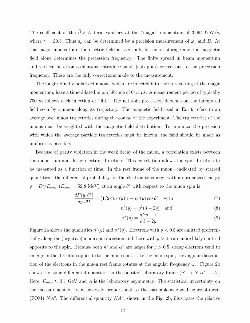
The coefficient of the ~β × ~E term vanishes at the “magic” momentum of 3.094 GeV/c,
where γ = 29.3. Thus aµ can be determined by a precision measurement of ωa and B. At
this magic momentum, the electric field is used only for muon storage and the magnetic
field alone determines the precession frequency. The finite spread in beam momentum
and vertical betatron oscillations introduce small (sub ppm) corrections to the precession
frequency. These are the only corrections made to the measurement.
The longitudinally polarized muons, which are injected into the storage ring at the magic
momentum, have a time-dilated muon lifetime of 64.4 µs. A measurement period of typically
700 µs follows each injection or “fill.” The net spin precession depends on the integrated
field seen by a muon along its trajectory. The magnetic field used in Eq. 6 refers to an
average over muon trajectories during the course of the experiment. The trajectories of the
muons must be weighted with the magnetic field distribution. To minimize the precision
with which the average particle trajectories must be known, the field should be made as
uniform as possible.
Because of parity violation in the weak decay of the muon, a correlation exists between
the muon spin and decay electron direction. This correlation allows the spin direction to
be measured as a function of time. In the rest frame of the muon—indicated by starred
quantities—the differential probability for the electron to emerge with a normalized energy
y = E∗/Emax (Emax = 52.8 MeV) at an angle θ∗ with respect to the muon spin is
dP (y, θ∗)dy dΩ
= (1/2π)n∗(y)[1− α∗(y) cos θ∗] with (7)
n∗(y) = y2(3− 2y) and (8)
α∗(y) =q
e
2y − 1
3− 2y. (9)
Figure 2a shows the quantities n∗(y) and α∗(y). Electrons with y < 0.5 are emitted preferen-
tially along the (negative) muon spin direction and those with y > 0.5 are more likely emitted
opposite to the spin. Because both n∗ and α∗ are larger for y > 0.5, decay electrons tend to
emerge in the direction opposite to the muon spin. Like the muon spin, the angular distribu-
tion of the electrons in the muon rest frame rotates at the angular frequency ωa. Figure 2b
shows the same differential quantities in the boosted laboratory frame (n∗ → N, α∗ → A).
Here, Emax ≈ 3.1 GeV and A is the laboratory asymmetry. The statistical uncertainty on
the measurement of ωa is inversely proportional to the ensemble-averaged figure-of-merit
(FOM) NA2. The differential quantity NA2, shown in the Fig. 2b, illustrates the relative
12

y0 0.1 0.2 0.3 0.4 0.5 0.6 0.7 0.8 0.9 1
Rel
ativ
e N
um
ber
(n
) o
r A
sym
met
ry (
A)
-0.2
0
0.2
0.4
0.6
0.8
1
n(y)
A(y)(y)α*
n (y)*
(a)Center-of-mass frame
y0 0.1 0.2 0.3 0.4 0.5 0.6 0.7 0.8 0.9 1
No
rmal
ized
nu
mb
er (
N)
or
Asy
mm
etry
(A
)
-0.2
0
0.2
0.4
0.6
0.8
1N
A
NA2
(b)Lab frame
FIG. 2: Relative number and asymmetry distributions versus electron fractional energy y in the
muon rest frame (left panel) and in the laboratory frame (right panel). The differential figure-of-
merit product NA2 in the laboratory frame illustrates the importance of the higher-energy electrons
in reducing the measurement statistical uncertainty.
weight by electron energy to the ensemble average FOM.
Because the stored muons are highly relativistic, the decay angles observed in the labora-
tory frame are greatly compressed into the direction of the muon momenta. The lab energy
of the relativistic electrons is given by
Elab = γ(E∗ + βp∗c cos θ∗) ≈ γE∗(1 + cos θ∗). (10)
Because the laboratory energy depends strongly on the decay angle θ∗, setting a laboratory
threshold Eth selects a range of angles in the muon rest frame. Consequently, the integrated
number of electrons above Eth is modulated at frequency ωa with a threshold-dependent
asymmetry. The integrated decay electron distribution in the lab frame has the form
Nideal(t) = N0 exp(−t/γτµ) [1− A cos(ωat + φ)] , (11)
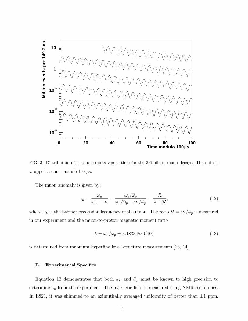
where N0, A and φ are all implicitly dependent on Eth. For a threshold energy of 1.8 GeV
(y ≈ 0.58 in Fig. 2b), the asymmetry is ≈ 0.4 and the average FOM is maximized. A
representative electron decay time histogram is shown in Fig. 3.
To determine aµ , we divide ωa by ωp, where ωp is the measure of the average magnetic
field seen by the muons. The magnetic field, measured using NMR, is proportional to the
free proton precession frequency, ωp.
13
sµTime modulo 1000 20 40 60 80 100
Mill
ion
eve
nts
per
149
.2 n
s
10-3
10-2
10-1
1
10
FIG. 3: Distribution of electron counts versus time for the 3.6 billion muon decays. The data is
wrapped around modulo 100 µs.
The muon anomaly is given by:
aµ =ωa
ωL − ωa
=ωa/ωp
ωL/ωp − ωa/ωp
=R
λ−R , (12)
where ωL is the Larmor precession frequency of the muon. The ratio R = ωa/ωp is measured
in our experiment and the muon-to-proton magnetic moment ratio
λ = ωL/ωp = 3.18334539(10) (13)
is determined from muonium hyperfine level structure measurements [13, 14].
B. Experimental Specifics
Equation 12 demonstrates that both ωa and ωp must be known to high precision to
determine aµ from the experiment. The magnetic field is measured using NMR techniques.
In E821, it was shimmed to an azimuthally averaged uniformity of better than ±1 ppm.
14

Improvements will be made in the re-shimming process with the aim of an even more uniform
field. To monitor the magnetic field during data collection, 366 fixed NMR probes are placed
around the ring to track the field in time. A trolley with 17 NMR probes will map the field
in the storage ring, in vacuum, several times per week. The trolley probes will be calibrated
with a special spherical water probe, which provides a calibration to the free proton spin
precession frequency ωp. The details are described later.
The experiment is run using positive muons owing to the higher cross section for π+
production from 8-GeV protons. In the ring, the decay positrons are detected in new,
segmented tungsten-scintillating-fiber calorimeters [15] where their energy and arrival time
are measured. The number of high-energy positrons above an energy threshold Eth as a
function of time is given by
N(t) = N0(Eth)e−t/γτ [1 + A(Eth) sin(ωat + φa(Eth))] . (14)
The uncertainty on ωa is given by
δωa
ωa
=
√2
ωaτµ
√NA
(15)
where the energy threshold Eth is chosen to optimize the quantity NA2.
The key to any precision measurement is the systematic errors. A summary of the
realized systematic errors from BNL E821 is given in Table II. Our goal is to improve the
net systematic error on both categories—ωa and ωp—to ≈ 0.07 ppm, each. The design of
the new experiment is based on a full consideration of items in this table, which will be
discussed in detail in the proposal. In some cases, R&D work will be required to develop
instrumentation to achieve the stated systematic goals.
15

σsyst ωp 1999 2000 2001 σsyst ωa 1999 2000 2001
(ppm) (ppm) (ppm) (ppm) (ppm) (ppm)
Inflector fringe field 0.20 - - Pile-Up 0.13 0.13 0.08
Calib. of trolley probes 0.20 0.15 0.09 AGS background 0.10 0.01 ‡Tracking B with time 0.15 0.10 0.07 Lost muons 0.10 0.10 0.09
Measurement of B0 0.10 0.10 0.05 Timing shifts 0.10 0.02 ‡µ-distribution 0.12 0.03 0.03 E-field/pitch 0.08 0.03 ‡Absolute calibration 0.05 0.05 0.05 Fitting/binning 0.07 0.06 ‡Others† 0.15 0.10 0.07 CBO 0.05 0.21 0.07
Beam debunching 0.04 0.04 ‡Gain changes 0.02 0.13 0.12
Total for ωp 0.4 0.24 0.17 Total for ωa 0.3 0.31 0.21
TABLE II: Systematic Errors from the E821 running periods in 1999, 2000 and 2001 [10–12]. CBO
stands for coherent betatron oscillations. The pitch correction comes from the vertical betatron
oscillations, since ~β · ~B 6= 0. The E-field correction is for the radial electric field seen by muons
with pµ 6= pmagic.
†Higher multipoles, the trolley frequency, temperature, and voltage response, eddy currents from
the kickers, and time-varying stray fields
‡In 2001 AGS background, timing shifts, E field and vertical oscillations, beam debunch-
ing/randomization, binning and fitting procedure together equaled 0.11 ppm
III. THE PHYSICS CASE FOR A NEW (g − 2) EXPERIMENT
In the first part of this section we present the standard model theory of the muon anoma-
lous magnetic moment (anomaly). Then we discuss physics beyond the standard model that
could contribute to the anomaly at a measurable level. The conclusion is that muon (g− 2)
will play a powerful role in the interpretation of new phenomena that might be discovered
at the LHC. If new phenomena are not discovered there, then muon (g − 2) becomes even
more important, since it would provide one of the few remaining ways to search for new
physics at the TeV scale.
The magnetic moment of the muon (or electron), which is aligned with its spin, is given
16
by
~µ = gq
2mµ,e
~s , g = 2︸ ︷︷ ︸Dirac
(1 + aµ) ; (16)
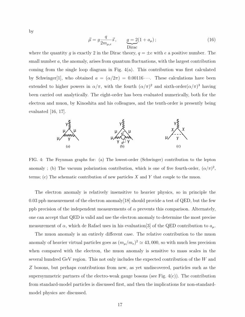
where the quantity g is exactly 2 in the Dirac theory, q = ±e with e a positive number. The
small number a, the anomaly, arises from quantum fluctuations, with the largest contribution
coming from the single loop diagram in Fig. 4(a). This contribution was first calculated
by Schwinger[1], who obtained a = (α/2π) = 0.00116 · · ·. These calculations have been
extended to higher powers in α/π, with the fourth (α/π)2 and sixth-order(α/π)3 having
been carried out analytically. The eight-order has been evaluated numerically, both for the
electron and muon, by Kinoshita and his colleagues, and the tenth-order is presently being
evaluated [16, 17].
(a) (b) (c)
γ
µγ γ
µγ
γµ
γ
µ
X X
Y
µ −e
+e
µ µ
FIG. 4: The Feynman graphs for: (a) The lowest-order (Schwinger) contribution to the lepton
anomaly ; (b) The vacuum polarization contribution, which is one of five fourth-order, (α/π)2,
terms; (c) The schematic contribution of new particles X and Y that couple to the muon.
The electron anomaly is relatively insensitive to heavier physics, so in principle the
0.03 ppb measurement of the electron anomaly[18] should provide a test of QED, but the few
ppb precision of the independent measurements of α prevents this comparison. Alternately,
one can accept that QED is valid and use the electron anomaly to determine the most precise
measurement of α, which de Rafael uses in his evaluation[3] of the QED contribution to aµ.
The muon anomaly is an entirely different case. The relative contribution to the muon
anomaly of heavier virtual particles goes as (mµ/me)2 ' 43, 000, so with much less precision
when compared with the electron, the muon anomaly is sensitive to mass scales in the
several hundred GeV region. This not only includes the expected contribution of the W and
Z bosons, but perhaps contributions from new, as yet undiscovered, particles such as the
supersymmetric partners of the electro-weak gauge bosons (see Fig. 4(c)). The contribution
from standard-model particles is discussed first, and then the implications for non-standard-
model physics are discussed.
17
The standard model value of aµ has three contributions from radiative processes: QED
loops containing leptons (e, µ, τ) and photons; loops containing hadrons in vacuum polariza-
tion loops where the e+e− pair in Fig 4(b) is replaced by hadrons; and weak loops involving
the weak gauge bosons W,Z, and Higgs such as is shown in Fig. 4(c) where X = W and
Y = ν, or X = µ and Y = Z. Thus
aµ(SM) = aµ(QED) + aµ(hadronic) + aµ(weak). (17)
Each of these contributions is discussed below.
A. The Standard-Model Value of aµ
1. QED and Weak Contributions
The QED and electroweak contributions to aµ are well understood. We take the numerical
values from reviews by de Rafael[3, 19] The QED contribution to aµ has been calculated
through four loops, with the leading five loop contributions estimated [16, 17]. The present
value is
aQEDµ = 116 584 718.09 (0.02)(0.14)(0.04)× 10−11 (18)
where the uncertainties are from the 4- and 5-loop QED contributions, and the value of α
taken from the electron (g − 2) value[3].
The electroweak contribution (shown in Fig. 5) is now calculated through two loops. The
single loop result
aEW(1)
µ =GF√
2
m2µ
8π2
10
3︸︷︷︸W
+1
3(1−4 sin2 θW )2 − 5
3︸ ︷︷ ︸Z
+ O(
m2µ
M2Z
logM2
Z
m2µ
)+
m2µ
M2H
∫ 1
0dx
2x2(2− x)
1− x +m2
µ
M2H
x2
= 194.8× 10⁻¹¹ , (19)
was calculated by five separate groups shortly after the Glashow-Salam-Weinberg theory
was shown by ’t Hooft to be renormalizable. With the present limit on the Higgs boson
mass, only the W and Z contribute at a measurable level.
18

µ νµ
W Wγ
µ
γ
Z0 µ
γ
Z0
f
f-
µ W
νµ νµ
γ
µ
γ G
W G
H
γ
(a) (b) (c) (d) (e)
FIG. 5: Weak contributions to the muon anomalous magnetic moment. Single-loop contributions
from (a) virtual W and (b) virtual Z gauge bosons. These two contributions enter with opposite
sign, and there is a partial cancellation. The two-loop contributions fall into three categories: (c)
fermionic loops which involve the coupling of the gauge bosons to quarks, (d) bosonic loops which
appear as corrections to the one-loop diagrams, and (e) a new class of diagrams involving the
Higgs where G is the longitudinal component of the gauge bosons. See Ref. [19] for details. The
× indicates the virtual photon from the magnetic field.
The two-loop weak contribution, (see Figs. 5(c-e) for examples) is negative, and the total
electroweak contribution is
aEWµ = 152(1)(2)× 10−11 (20)
where the first error comes from hadronic effects in the second-order electroweak diagrams
with quark triangle loops, and the latter comes from the uncertainty on the Higgs mass[3, 19].
The leading logs for the next-order term have been shown to be small. The weak contribution
is about 1.3 ppm of the anomaly, so the experimental uncertainty on aµ of ±0.54 ppm now
probes the weak scale of the standard model.
2. The Hadronic Contribution
The hadronic contribution to aµ is about 60 ppm of the total value. The lowest-order
diagram shown in Fig. 6(a) dominates this contribution and its error, but the hadronic
light-by-light contribution Fig. 6(e) is also important.
The energy scale for the virtual hadrons is of order mµc2, well below the perturbative
region of QCD. Thus it must be calculated from the dispersion relation shown pictorially in
19

µ
γ
Hµ
γ
e Hµ
γ
Hµ
γ
H H
µ
γ
H
(a) (b) (c) (d) (e)
FIG. 6: The hadronic contribution to the muon anomaly, where the dominant contribution comes
from the lowest-order diagram (a). The hadronic light-by-light contribution is shown in (e).
Fig. 7,
ahad;LOµ =
(αmµ
3π
)2 ∫ ∞
4m2π
ds
s2K(s)R(s), where R ≡ σtot(e
+e− → hadrons)
σ(e+e− → µ+µ−), (21)
using the measured cross sections for e+e− → hadrons as input, where K(s) is a kinematic
factor ranging from -0.63 at s = 4m2π to 1 at s = ∞. This dispersion relation relates the
bare cross section for e+e− annihilation into hadrons to the hadronic vacuum polarization
contribution to aµ. Because the integrand contains a factor of s−2, the values of R(s)
at low energies (the ρ resonance) dominate the determination of ahad;LOµ . This is shown
in Fig. 8, where the left-hand chart gives the relative contribution to the integral for the
different energy regions, and the right-hand gives the contribution to the error squared on
the integral. The contribution is dominated by the two-pion final state, but other low-energy
multi-hadron cross sections are also important.
ISR
*
(a) (b) (c)
γ
−e
+e
hγ
−e
+e
h
γγ
γ
µh
*
FIG. 7: (a) The “cut” hadronic vacuum polarization diagram; (b) The e+e− annihilation into
hadrons; (c) Initial state radiation accompanied by the production of hadrons.
These data for e+e− annihilation to hadrons are also important as input into the deter-
mination of αs(MZ) and other electroweak precision measurements, including the limit on
20
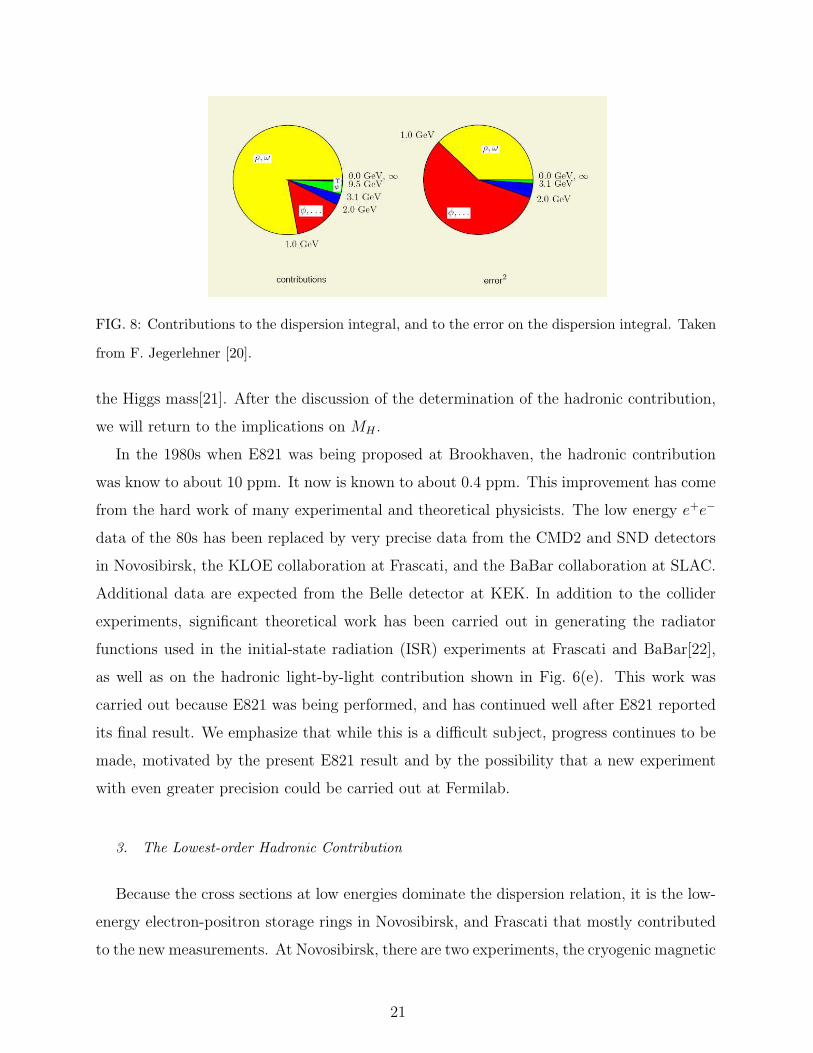
FIG. 8: Contributions to the dispersion integral, and to the error on the dispersion integral. Taken
from F. Jegerlehner [20].
the Higgs mass[21]. After the discussion of the determination of the hadronic contribution,
we will return to the implications on MH .
In the 1980s when E821 was being proposed at Brookhaven, the hadronic contribution
was know to about 10 ppm. It now is known to about 0.4 ppm. This improvement has come
from the hard work of many experimental and theoretical physicists. The low energy e+e−
data of the 80s has been replaced by very precise data from the CMD2 and SND detectors
in Novosibirsk, the KLOE collaboration at Frascati, and the BaBar collaboration at SLAC.
Additional data are expected from the Belle detector at KEK. In addition to the collider
experiments, significant theoretical work has been carried out in generating the radiator
functions used in the initial-state radiation (ISR) experiments at Frascati and BaBar[22],
as well as on the hadronic light-by-light contribution shown in Fig. 6(e). This work was
carried out because E821 was being performed, and has continued well after E821 reported
its final result. We emphasize that while this is a difficult subject, progress continues to be
made, motivated by the present E821 result and by the possibility that a new experiment
with even greater precision could be carried out at Fermilab.
3. The Lowest-order Hadronic Contribution
Because the cross sections at low energies dominate the dispersion relation, it is the low-
energy electron-positron storage rings in Novosibirsk, and Frascati that mostly contributed
to the new measurements. At Novosibirsk, there are two experiments, the cryogenic magnetic
21
detector (CMD2), and the spherical neutral detector (SND) which has no magnetic field.
Both of these experiments have measured the hadronic cross section in a traditional energy
scan. At Frascati, ISR (often called “radiative return”) has been used, where the accelerator
is operated at around 1 GeV (mostly on the φ resonance), using hadronic events accompanied
by an initial-state (ISR) photon (see Fig. 7(c)) to measure the hadronic cross-section. More
recently the BaBar experiment has used ISR to measure the hadronic cross sections, and
their data on multi-hadron final states have been published. The BaBar data, taken at
the PEP2 collider, differ from the lower-energy experiments at KLOE, since the initial-state
photon is quite energetic and easily detected. The Belle experiment at KEK is also beginning
to look at ISR data, and we assume that they too will join this effort.
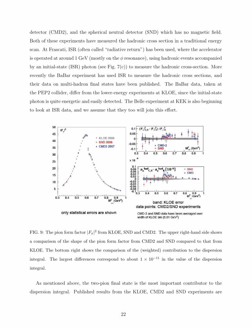
FIG. 9: The pion form factor |Fπ|2 from KLOE, SND and CMD2. The upper right-hand side shows
a comparison of the shape of the pion form factor from CMD2 and SND compared to that from
KLOE. The bottom right shows the comparison of the (weighted) contribution to the dispersion
integral. The largest differences correspond to about 1 × 10⁻¹¹ in the value of the dispersion
integral.
As mentioned above, the two-pion final state is the most important contributor to the
dispersion integral. Published results from the KLOE, CMD2 and SND experiments are
22

shown in Fig. 9. It is traditional to report the pion form factor Fπ, defined by
σe+e−→π+π− =πα2
3sβ3
π|Fπ|2 , (22)
which is shown below for KLOE, CMD2 and SND.
A recent analysis [27] gives:
ahvpµ = (6 908± 39exp ± 19rad ± 7QCD)× 10−11 . (23)
which represents the effort of many experimental groups. Important earlier global analyses
include those of HMNT [23], Davier [24], Jegerlehner[25] and Hocker and Marciano[26].
Following de Rafael, we use the recent analysis of Zhang [27], which however does not
include the new results from the KLOE experiment [28] which were published after Zhang’s
review. The next-order hadronic contribution shown in Fig. 6(b-d) can also be determined
from a dispersion relation, and the result is
ahvp(nlo)µ = (−97.9± 0.9exp ± 0.3rad )× 10−11 . (24)
4. BaBar e+e− → π+π− Data
In September 2008, preliminary results from the ππ final state using the radiative return
method were reported by the BaBar collaboration [29]. At the time of this proposal, they
remain preliminary and cannot yet be included in the dispersion relation. Davier, in his 30
January, 2009 seminar at Fermilab, announced that a systematic problem was discovered
in the threshold region, which affects the previously announced cross section measurements
in the higher-mass region. The BaBar Collaboration is completing their work now and will
make final results available in the next few months. Davier pointed out that the uncertainty
on the lowest-order hadronic contribution from “existing e+e− data (all experiments) can
reach a precision δaµ = 25×10−11” and he expressed optimism that “remaining discrepancies
will be brought close to quoted systematic uncertainties.”
5. ahad;LOµ from Hadronic τ decay
The value of ahad;LOµ from threshold up to mτ could in principle be obtained from hadronic
τ− decays (See Fig. 6), provided that the necessary isospin corrections are known. This
23

was first demonstrated by Almany, Davier and Hocker [30]. Hadronic τ decays to an even
number of pions such as τ− → π−π0ντ , which in the absence of second-class currents goes
through the vector part of the weak current, can be related to e+e− annihilation into π+π−
through the CVC hypothesis and isospin conservation (see Fig. 10) [30–32]. The τ -data
only contain an isovector piece, and the isoscalar piece present in e+e− annihilation has to
be put in “by hand” to evaluate ahad;LOµ . At present, most authors [3, 20, 23] conclude that
there are unresolved issues such as the isospin breaking corrections, which make it difficult
to use the τ data on an equal footing with the e+e− data .
-ττ
W-
ν
h
(b)
+e
-e
γh
(a)
FIG. 10: e+e− annihilation into hadrons (a), and hadronic τ decay (b).
6. The Hadronic Light-by-Light Contribution
The hadronic light-by-light contribution, (Fig. 6(e)) cannot at present be determined
from data, but rather must be calculated using hadronic models that correctly reproduce
the properties of QCD. A number of authors have calculated portions of this contribution,
and recently a compilation of all contributions has become available from Prades, de Rafael
and Vainshtein [33], which has been agreed to by authors from each of the leading groups
working in this field. They obtain
aHLbLµ = (105± 26)× 10−11 . (25)
Additional work on this contribution is underway at Minnesota [34].
B. Summary of the Standard Model Value and Comparison with Experiment
Following de Rafael [3], the standard-model value obtained from the published e+e− data
from KLOE, CMD2 and SND, and published data from BaBar for the multi-pion final states
is used to determine ahvpµ and ahvp(nlo)
µ . A summary of these values is given in Table III.
24

TABLE III: Standard model contributions to the muon anomaly. Taken from de Rafael[3].
Contribution Result in 10−11 units
QED (leptons) 11 6584 718.09± 0.14± 0.04α
HVP(lo) 6 908± 39exp ± 19rad ± 7pQCD
HVP(ho) −97.9± 0.9exp ± 0.3rad
HLxL 105± 26
EW 152± 2± 1
Total SM 116 591 785± 51
This standard-model value is to be compared with the combined a+µ and a−µ values from
E821 [2]:
aE821µ = (116 592 080± 63)× 10−11 (0.54 ppm), (26)
aSMµ = (116 591 785± 51)× 10−11 (0.44 ppm) (27)
which give a difference of
∆aµ(E821− SM) = (295± 81)× 10−11 . (28)
This comparison is shown graphically in Fig. 11.
S−M
The
ory
X 1
0−11
µ++µ
µ−
116
591
000
116
592
000
116
593
000
116
594
000
116
595
000
116
590
000
(13 ppm) E821 (97)
(9.4 ppm)
(10 ppm)
+
CERN
E821 (98)(5 ppm)
(0.7 ppm)E821 (01)(0.7 ppm)E821 (00)E821 (99)(1.3 ppm)
World Average
CERN µ
µ+
µ−
µ+
a µ
FIG. 11: Measurements of aµ along with the standard-model value given above.
25

This difference of 3.6 standard deviations is tantalizing, but we emphasize that whatever
the final agreement between the measured and standard-model value turns out to be, it will
have significant implications on the interpretation of new phenomena that might be found
at the LHC and elsewhere. This point is discussed in detail below.
The present theoretical error [3] of±51×10−11 (0.44 ppm) is dominated by the±39×10−11
uncertainty on the lowest-order hadronic contribution and the ±26 × 10−11 uncertainty on
the hadronic light-by-light contribution. As mentioned above, Davier suggested that the
uncertainty on the lowest-order hadronic contribution could be reduced to 25 × 10−11 with
“potentially existing data”. Future work described below could lower this further, and
along with future theoretical progress on the hadronic light-by-light contribution, the total
standard-model error could reach 30× 10−11.
With the proposed experimental error of ±16× 10−11, the combined uncertainty for the
difference between theory and experiment would be ±34 × 10−11, which is to be compared
with the ±81× 10−11 in Eq. 28.
1. R(s) Measurements and the Higgs Mass, MH
If the hadronic cross section that enters into the dispersion relation of Eq. 21 were to
increase significantly from the value obtained in the published papers of CMD2, SND and
KLOE, then as pointed out by Passera, Marciano and Sirlin [21], it would have significant
implications for the limit on the mass of the Higgs boson. The value of ∆α(5)had(MZ) depends
on the same measured cross-sections that enter into Eq. 21,
∆α(5)had(MZ) =
M2Z
4απ2P
∫ ∞
4m2π
dsσ(s)
M2Z − s
. (29)
The present bound of MH ≤ 150 GeV (95% C.L.) changes if ∆αhad(MZ) changes. Assuming
that the hadronic contribution to aµ is increased by the amount necessary to remove the
difference between the experimental and theoretical values of aµ, the effect on MH is to
move the upper bound down to ' 130 GeV. Given the experimental limit MH > 114.4 GeV
(95% C.L.), this significantly narrows the window for the Higgs mass. The details depend on
the s-region assumed to be incorrect in the hadronic cross section. A much more complete
discussion is given in Ref. [21].
26
C. Expected Improvements in the Standard Model Value
Much experimental and theoretical work is going on worldwide to refine the hadronic con-
tribution. One reflection of this effort is the workshop held in Glasgow[35], which brought
together 27 participants who are actively working on parts of this problem, including the be-
yond the standard model implications of aµ . These participants represented many additional
collaborators.
In the near term there will be two additional results from KLOE, in addition to the final
BaBar result. An upgrade at Novosibirsk is now underway.
• Novosibirsk: The CMD2 collaboration has upgraded their detector to CMD3, and
the VEPP2M machine has been upgraded to VEPP-2000. The maximum energy has
been increased from√
s = 1.4 GeV to 2.0 GeV. These upgrades will permit the cross
section to be measured from threshold to 2.0 GeV using an energy scan, filling in
the energy region between 1.4 GeV, where the CMD2 scan ended, up to 2.0 GeV,
the lowest energy point reached by the BES collaboration in their measurements. See
Fig. 8 for the present contribution to the overall error from this region. The SND
detector has also been upgraded. Engineering runs will take place in 2009, with data
collection beginning in late 2009 or 2010. They will also take data at 2 GeV, using
ISR, which will provide data between the PEP2 energy at the Υ(4s) and the 1 GeV φ
energy at the DAφNE facility in Frascati.
• KLOE: The KLOE collaboration has measured the hadronic cross section using
initial-state radiation (ISR) to lower the CM energy from the φ where DAφNE op-
erates. Significant data have now been published. Several additional analyses are in
progress: a measurement of the pion form factor from the bin by bin ratio of π+π−γ
to µ+µ−γ spectrum, (as is being done with the BaBar analysis) large-angle ISR data;
and ISR data taken off of the φ resonance, with a different data set, analysis selection,
and background conditions.
• BaBar: As discussed above, the BaBar collaboration is several months from reporting
the final analysis of their π+π− ISR data. They have significantly more data, but at
present, no member of the collaboration has taken on the leadership of that analysis
effort.
27
• Belle: Some work on ISR measurements of R(s) is going on but at present they are
not nearly as far along as BaBar.
• Calculations on the Lattice - Lowest-Order: With the increased computer power
available for lattice calculations, it may be possible for lattice calculations to contribute
to our knowledge of the lowest order hadronic contribution. Blum has performed a
proof-of-principle quenched calculation on the lattice.[36, 37] Several groups, UKQCD
(Edinburg), DESY-Zeuthen (Renner and Jansen), and the LSD (lattice strong dynam-
ics) group in the US are all working on the lowest-order contribution.
• Calculations on the Lattice - Hadronic light-by-light: The hadronic light-
by-light contribution has a magnitude of (105 ± 26) × 10−11, ∼ 1 ppm of aµ. A
modest calculation on the lattice would have a large impact. There are two separate
efforts to formulate the hadronic light-by-light calculation on the lattice. Blum and his
collaborators at BNL and RIKEN (RBC collaboration) are working on the theoretical
framework for a lattice calculation of this contribution, and are calculating the QED
light-by-light contribution as a test of the program.[38]
D. Physics Beyond the Standard Model
For many years, the muon anomaly has played an important role in constraining physics
beyond the standard model [39–42]. The 1260 citations to the major E821 papers [2, 10–12],
with 164 in 2008, demonstrates that this role continues.
In this section, we discuss how the muon anomaly provides a unique window to search
for physics beyond the standard model. If new physics is discovered at the LHC, then aµ
will play an important role in sorting out the interpretation of those discoveries. In the
sections below, examples of constraints placed on various models that have been proposed
as extensions of the standard model are discussed. However, perhaps the ultimate value of
an improved limit on aµ, will come from its ability to constrain the models that we have yet
invented.
If the LHC produces the standard model Higgs and nothing else, then the only tools
available to probe the high-energy frontier will be precision measurements of aµ or other
weak processes, together with searches for charged lepton flavor violation, electric dipole
28

moments, and rare decays.
The role of (g − 2) as a discriminator between very different standard model extensions
is well illustrated by a relation discussed by Czarnecki and Marciano [40] that holds in a
wide range of models: If a new physics model with a mass scale Λ contributes to the muon
mass δmµ(N.P.), it also contributes to aµ , and the two contributions are related as
aµ(N.P.) = O(1)×(
mµ
Λ
)2
×(
δmµ(N.P.)
mµ
). (30)
The ratio C(N.P.) ≡ δmµ(N.P.)/mµ is typically between O(α/4π) (for perturbative con-
tributions to the muon mass) and O(1) (if the muon mass is essentially due to radiative
corrections). Hence the contributions to aµ are highly model dependent.
A variety of models with radiative muon mass generation at some scale Λ have been
discussed in [40], including extended technicolor or generic models with naturally vanishing
bare muon mass. In these models the ratio C(N.P.) ' 1 and the new physics contribution
to aµ can be very large,
aµ(Λ) ' m2µ
Λ2' 1100× 10−11
(1 TeV
Λ
)2
. (31)
and the difference Eq. 3 can be used to place a lower limit on the new physics mass scale,
which is in the few TeV range [43]. In models with extra weakly interacting gauge bosons
Z ′, W ′, e.g. certain models with extra dimensions, C(N.P.) = O(α/4π), and a difference
as large as Eq. 3 is very hard to accommodate unless the mass scale is very small, of the
order of MZ . In a model with δ = 1 (or 2) universal extra dimensions, other measurements
already imply a lower bound of 300 (or 500) GeV on the masses of the extra states, and the
one-loop contributions to aµ are correspondingly small,
aµ(UED) ' −5.8× 10⁻¹¹(1 + 1.2δ)SKK (32)
with |SKK|<∼1 [44]. Many other models with extra weakly interacting particles give similar
results [45]. If any of these are realized in Nature, the new measurement of aµ would be
expected to agree with the standard model value within approximately ±34 × 10−11, the
projected sensitivity of the combined standard model plus experiment sensitivity.
Supersymmetric models lie in between these two extremes. Were they to exist, muon
(g − 2) would have substantial sensitivity to the supersymmetric particles. Compared
to generic perturbative models, supersymmetry provides an enhancement to C(SUSY) =
29

O(tan βα/4π) and to aµ(SUSY) by a factor tan β (the ratio of the vacuum expectation
values of the two Higgs fields). The SUSY diagrams for the magnetic dipole moment, the
electric dipole moment, and the lepton-number violating conversion process µ → e in the
field of a nucleus are shown pictorially in Fig. 12. In a model with SUSY masses equal to Λ
the supersymmetric contribution to aµ is given by [40]
aµ(SUSY) ' sgn (µ) 130× 10−11 tan β(
100 GeV
Λ
)2
(33)
which indicates the dependence on tan β, and the SUSY mass scale, as well as the sign of
the SUSY µ-parameter. Thus muon (g − 2) is sensitive to any SUSY model with large
tan β. Conversely, SUSY models with Λ in the few hundred GeV range could provide an
explanation of the deviation in Eq. 3.
FIG. 12: The supersymmetric contributions to the anomaly, and to µ → e conversion, showing the
relevant slepton mixing matrix elements. The MDM and EDM give the real and imaginary parts
of the matrix element, respectively. The × indicates a chirality flip.
In the next decade, LHC experiments will for the first time directly probe physics at the
TeV scale. This scale appears to be a crucial scale in particle physics. It is linked to elec-
troweak symmetry breaking, and many arguments indicate that radically new concepts such
as supersymmetry, extra dimensions, technicolor, or other new interactions, could be real-
ized at this scale. Furthermore, cold dark matter particles could have weak-scale/TeV-scale
masses, and if it exists, models of Grand Unification prefer the existence of supersymmetry
at the TeV scale. TeV-scale physics could be very rich, and the LHC is designed to discover
physics beyond the standard model. This will make the precision experiments such as muon
(g − 2) and searches for charged lepton flavor violation complementary partners
In the quest to identify the nature of TeV-scale physics and to answer questions related to
e.g. electroweak symmetry breaking and Grand Unification, we need to combine and cross-
check information from the LHC with information from as many complementary experiments
30

as possible. This need is highlighted by the unprecedented complexity of the LHC accelerator
and experiments, the involved initial and final states, and the huge backgrounds at the
LHC. In all these respects, an improved muon (g − 2) measurement is needed to provide
an indispensable complement.
In the following we discuss in more detail how aµ will be useful in understanding TeV-
scale physics in the event that the LHC established the existence of physics beyond the
standard model [46].
1. aµ as a benchmark for models of new physics
It has been established that the LHC is sensitive to virtually all proposed weak-scale
extensions of the standard model, ranging from supersymmetry (SUSY) to extra dimensions,
little Higgs models and others. However, even if the existence of physics beyond the standard
model is established, it will be far from easy for the LHC alone to identify which of the
possible alternatives is realized. The measurement of aµ to 16×10−11 will be highly valuable
in this respect since it will provide a benchmark and stringent selection criterion that can
be imposed on any model that is tested at the LHC.
For example, a situation is possible where the LHC finds many new heavy particles which
are compatible with both minimal-supersymmetric and universal-extra-dimension model
predictions [47]. The muon (g − 2) would especially aid in the selection since UED models
predict a tiny effect to aµ , while SUSY effects are usually much larger.
Likewise, within SUSY itself there are many different well-motivated scenarios that are
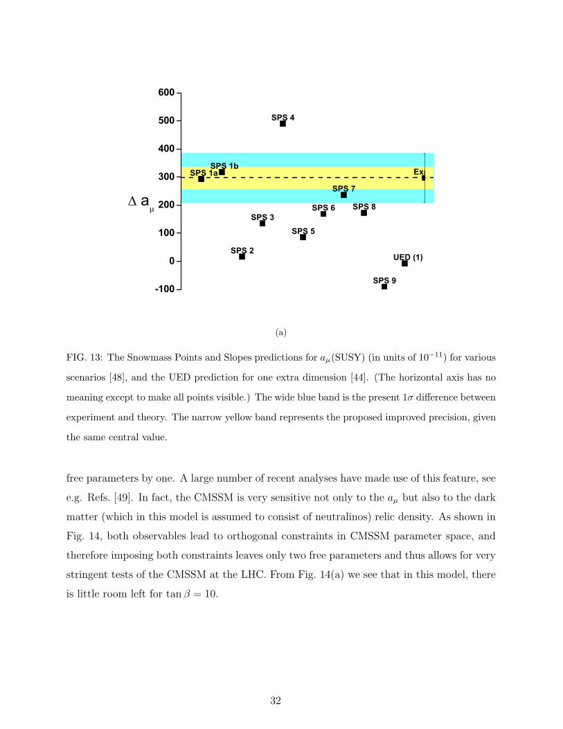
not always easy to distinguish at the LHC. Fig. 13 shows a graphical distribution of the 10
Snowmass Points and Slopes model benchmark predictions [48] for aµ(SUSY). They range
considerably and can be positive and negative, due to the factor sgn(µ) in Eq. 33, where this
sign would be particularly difficult to determine at LHC, even if SUSY were to be discovered.
The discriminating power of an improved (g− 2) measurement—even if the actual value of
∆aµ turned out to be smaller—is evident from Fig. 13.
A final example concerns the restriction of special, highly constrained models of new
physics such as the constrained MSSM (CMSSM). The CMSSM has only four free con-
tinuous parameters. One precise measurement such as the future determination of ∆aµ
effectively fixes one parameter as a function of the others and thus reduces the number of
31
SPS 1aSPS 1b
SPS 2
SPS 3
SPS 4
SPS 5
SPS 6
SPS 7
SPS 8
SPS 9
UED (1)
Expt-SM
-100
0
100
200
300
400
500
600
a
(a)
FIG. 13: The Snowmass Points and Slopes predictions for aµ(SUSY) (in units of 10−11) for various
scenarios [48], and the UED prediction for one extra dimension [44]. (The horizontal axis has no
meaning except to make all points visible.) The wide blue band is the present 1σ difference between
experiment and theory. The narrow yellow band represents the proposed improved precision, given
the same central value.
free parameters by one. A large number of recent analyses have made use of this feature, see
e.g. Refs. [49]. In fact, the CMSSM is very sensitive not only to the aµ but also to the dark
matter (which in this model is assumed to consist of neutralinos) relic density. As shown in
Fig. 14, both observables lead to orthogonal constraints in CMSSM parameter space, and
therefore imposing both constraints leaves only two free parameters and thus allows for very
stringent tests of the CMSSM at the LHC. From Fig. 14(a) we see that in this model, there
is little room left for tan β = 10.
32

100 200 300 400 500 600 700 800 900 10000
100
200
300
400
500
600
700
800
100 200 300 400 500 600 700 800 900 10000
100
200
300
400
500
600
700
800
m0
(GeV
)
m1/2 (GeV)
tan β = 10 , µ > 0
mh = 114 GeV
mχ± = 104 GeV
(a)
100 200 300 400 500 600 700 800 900 10000
100
200
300
400
500
600
700
800
100 200 300 400 500 600 700 800 900 10000
100
200
300
400
500
600
700
800
m0
(GeV
)
m1/2 (GeV)
tan β = 10 , µ > 0
mh = 114 GeV
mχ± = 104 GeV
(b)
100 200 300 400 500 600 700 800 900 10000
100
200
300
400
500
600
700
800
100 200 300 400 500 600 700 800 900 10000
100
200
300
400
500
600
700
800
m0
(GeV
)
m1/2 (GeV)
tan β = 10 , µ > 0
mh = 114 GeV
mχ± = 104 GeV
(c)
100 1000 15000
1000
100 1000 15000
1000
m0
(GeV
)
m1/2 (GeV)
tan β = 40 , µ > 0
mh = 114 GeV
mχ± = 104 GeV
(d)
100 1000 15000
1000
100 1000 15000
1000
m0
(GeV
)
m1/2 (GeV)
tan β = 40 , µ > 0
mh = 114 GeV
mχ± = 104 GeV
(e)
100 1000 15000
1000
100 1000 15000
1000
m0
(GeV
)m1/2 (GeV)
tan β = 40 , µ > 0
mh = 114 GeV
mχ± = 104 GeV
(f)
FIG. 14: The m0(scalar mass)–m1/2(gaugino mass) plane of the CMSSM parameter space for
tanβ = (10; 40), A0 = 0, sgn(µ) = + :
(a;d) The ∆a(today)µ = 295(81) × 10−11 between experiment and standard-model theory is from
Ref. [3]. The brown wedge on the lower right is excluded by the requirement the dark matter be
neutral. Direct limits on the Higgs and chargino χ± masses are indicated by vertical lines, with the
region to the left excluded. Restrictions from the WMAP satellite data are shown as a light-blue
line. The (g − 2) 1 and 2-standard deviation boundaries are shown in purple. The green region is
excluded by b → sγ. (b;e) The plot with ∆aµ = 295(39)× 10−11. (c;f) The same errors as (b), but
∆aµ = 0. (Figures courtesy of K. Olive, following Ref. [50])
2. aµ is sensitive to quantities that are difficult to measure at the LHC
As a hadron collider, the LHC is particularly sensitive to colored particles. In contrast,
aµ is particularly sensitive to weakly interacting particles that couple to the muon and to
33

new physics effects on the muon mass, see Eq. 30.
For unraveling the mysteries of TeV-scale physics it is not sufficient to determine which
type of new physics is realized, but it is necessary to determine model parameters as pre-
cisely as possible. Here the complementarity between the LHC and precision experiments
such as aµ becomes particularly important. A difficulty at the LHC is the very indirect
relation between LHC observables (cross sections, mass spectra, edges, etc) and model
parameters such as masses and couplings, let alone more underlying parameters such as
supersymmetry-breaking parameters or the µ-parameter in the MSSM. Generally, the LHC
Inverse problem [51] states that several different points in the supersymmetry parameter
space can give rise to indistinguishable LHC signatures. It has been shown that a promising
strategy is to determine the model parameters by performing a global fit of a model such
as the MSSM to all available LHC data. However, recent investigations have revealed that
in this way typically a multitude of almost degenerate local minima of χ2 as a function of
the model parameters results [52]. Independent observables such as the ones available at
the proposed International Linear Collider [53] or aµwill be highly valuable to break such
degeneracies, and in this way to unambiguously determine the model parameters.
In the following we provide further examples for the complementarity of LHC and aµ
for the well-studied case of the MSSM. The LHC has only a weak sensitivity to two central
parameters: the sign of the µ-parameter and tan β, the ratio of the two Higgs vacuum
expectation values. According to Eq. 33 the MSSM contributions to aµ are highly sensitive
to both of these parameters. Therefore, a future improved aµ measurement has the potential
to establish a definite positive or negative sign of the µ-parameter in the MSSM, which would
be a crucial piece of information.
In the event that SUSY is discovered, we give an illustration of a tan β measurement
and reconsider the case discussed in Ref. [52], assuming that the MSSM reference point
SPS1a [48] is realized at LHC. Using the comprehensive LHC-analysis of [52], tan β can
be determined only rather poorly to tan βLHC fit = 10.0 ± 4.5. In such a situation one can
study the MSSM prediction for aµ as a function of tan β (all other parameters are known
from the global fit to LHC data) and compare it to the measured value, in particular after
an improved measurement. As can be seen from Fig. 15, using today’s value for aµ would
improve the determination of tan β, but the improvement will be even more impressive after
a future more precise aµ measurement. The limits on tan β are: E821 tan β = 9.8+3.9−3.4; FNAL
34
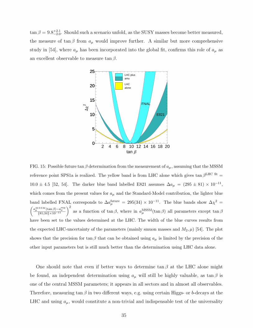
tan β = 9.8+2.1−2.0. Should such a scenario unfold, as the SUSY masses become better measured,
the measure of tan β from aµ would improve further. A similar but more comprehensive
study in [54], where aµ has been incorporated into the global fit, confirms this role of aµ as
an excellent observable to measure tan β.
LHC plusamu
LHCalone
2 4 6 8 10 12 14 16 18 2000
55
1010
1515
2020
2525
tan Β
DΧ
2 FNAL
E821
FIG. 15: Possible future tanβ determination from the measurement of aµ , assuming that the MSSM
reference point SPS1a is realized. The yellow band is from LHC alone which gives tanβLHC fit =
10.0 ± 4.5 [52, 54]. The darker blue band labelled E821 assumes ∆aµ = (295 ± 81) × 10−11,
which comes from the present values for aµ and the Standard-Model contribution, the lighter blue
band labelled FNAL corresponds to ∆afutureµ = 295(34) × 10−11. The blue bands show ∆χ2 =(
aMSSMµ (tan β)−aexp
µ
81;34×10−11
)2
as a function of tanβ, where in aMSSMµ (tanβ) all parameters except tanβ
have been set to the values determined at the LHC. The width of the blue curves results from
the expected LHC-uncertainty of the parameters (mainly smuon masses and M2, µ) [54]. The plot
shows that the precision for tanβ that can be obtained using aµ is limited by the precision of the
other input parameters but is still much better than the determination using LHC data alone.
One should note that even if better ways to determine tan β at the LHC alone might
be found, an independent determination using aµ will still be highly valuable, as tan β is
one of the central MSSM parameters; it appears in all sectors and in almost all observables.
Therefore, measuring tan β in two different ways, e.g. using certain Higgs- or b-decays at the
LHC and using aµ , would constitute a non-trivial and indispensable test of the universality
35

of tan β and thus of the structure of the MSSM.
At the 2007 Glasgow (g − 2) Workshop [35], Martin and Wells presented an update of
their so-called “superconservative analysis” [56], where a very conservative 5σ band around
the observed difference Eq. 3 and the general supersymmetric standard model are considered.
Surprisingly, it could be shown that even this mild assumption leads to regions of parameter
space which are excluded by (g−2) and nothing else. Hence, (g−2) provides complementary
information to collider, dark matter, or other low-energy observables. An improved (g − 2)
measurement will be very useful—independent of the actual numerical result.
In a similar spirit, Berger, Gainer, Hewett and Rizzo [57] discussed “supersymmetry
without prejudice.” First a large set of supersymmetry parameter points (“models”) in a
19-dimensional parameter space was identified, which was in agreement with many important
existing experimental and theoretical constraints. Then the implications for observables such
as (g − 2) were studied. The result for (g − 2) was rather similar to Fig. 13, although
the context was far more general: the entire range aSUSYµ ∼ (−100 . . . + 300) × 10−11 was
populated by a reasonable number of “models.” Therefore, a precise measurement of (g−2)
to ±16×10−11 will be a crucial way to rule out a large fraction of models and thus determine
supersymmetry parameters.
The anomalous magnetic moment of the muon is sensitive to contributions from a wide
range of physics beyond the standard model. It will continue to place stringent restrictions
on all of the models, both present and yet to be written down. Assuming that we will be so
fortunate as to discover new phenomena in the LHC era, aµ will constitute an indispensable
tool to discriminate between very different types of new physics, especially since it is highly
sensitive to parameters which are difficult to measure at the LHC. If we are unfortunate,
then it represents one of the few ways to probe beyond the standard model. In either case,
it will play an essential and complementary role in the quest to understand physics beyond
the standard model at the TeV scale. This prospect is what motivates our collaboration to
push forward with a new measurement.
36

IV. A NEW (g − 2) EXPERIMENT
A. Scientific Goal
The E821 results were based on three ∼ 2-month-long running periods in 1999, 2000, and
2001. A total of 8.55× 10⁹ events were included in the final fitted samples. Combined, this
leads to a relative statistical uncertainty of 0.46 ppm. The systematic uncertainties were, in
general, reduced in each running year, and a final combined averages for the magnetic field
measurement (0.17 ppm) and spin-precession analysis (0.21 ppm) were combined in quadra-
ture with the statistical error to obtain the final overall relative uncertainty of 0.54 ppm. In
absolute units, the experimental uncertainty on aµ is 63× 10−11.
The goal of the New (g − 2) Experiment is a precision improvement on aµ by a factor
of 4 to δaµ = 16 × 10−11, (0.14 ppm). This is an arrived at by assuming roughly equal
statistical and systematic uncertainty goals. At δaµ = 16 × 10−11, the uncertainty will be
well below the theoretical error for the seeable future. In consultation with theorists who
evaluate the SM contributions, we estimate that improved and larger HVP input data sets
will reduce the uncertainty from 51 to 30 in 10−11 units. Our experimental precision will
be well below theory, barring unforseen breakthroughs. The uncertainty on the comparison
between experiment and theory, ∆aµ , will be reduced to 34×10−11. This low-energy precision
SM test will provide a powerful discriminator of new physics models.
An improvement by a factor of 4 is both scientifically compelling and technically achiev-
able. To do so in less than 2 years of running, will require use of 6/20 of the Booster batches,
each subdivided fourfold leading to 18 Hz of storage ring fills (4 times the fill frequency at
BNL). The use of a long decay beamline, with true-forward decay kinematics and an open
inflector magnet, will serve to improve the muon storage efficiency per proton by a factor of
more than 6. A significant reduction in background will result from the long beamline. The
design of the experiment aims at a systematic error reduction by an overall factor of 3. The
plan described below will achieve these stated goals.
B. Key Elements to a New Experiment
The New (g−2) Experiment relies on the following improvements compared to the BNL
E821 Experiment:
37

1. Increasing the stored muon flux per incident proton,
2. Increasing the fill frequency (lowers the instantaneous rate),
3. Decreasing the hadron-induced flash at injection,
4. Improving the stored muon beam dynamics with a better kick into the ring and with
a damping scheme to reduce coherent betatron oscillations,
5. Improving the storage ring field uniformity and the measurement and calibration sys-
tem,
6. Increasing the detector segmentation to reduce the instantaneous rate.
Items 1− 3 will be realized by a clever use of the existing FNAL accelerator complex. A
single 8-GeV Booster batch will be injected into the Recycler, where it will be subdivided
into 4 bunches; 6 of the 20 batches per 15 Hz Booster cycle provide 24 individual bunches of
1012 protons. Each bunch is directed to the existing antiproton target to produce 3.1 GeV/c
positive pions, which will be focussed by the existing lithium lens system and a new pulsed
dipole magnet into the AP2 transfer line. The quadrupole density in the 270-m long AP2
line will be increased to reduce the beta function and consequently capture and transport a
high fraction of forward-decay muons. The muon beam will go around the Debuncher ring
for nearly one full turn, then be extracted into the existing AP3 channel back toward the
AP0 building. A new, short, transfer line will direct the beam into the storage ring through
a new open-ended inflector magnet. The storage ring will be located in a new building
near AP0 where ample cryo and power services are available nearby. In subsection IVC we
discuss how the background from the injection flash will be reduced.
Item 4 will be approached by optimization of the storage ring kicker pulse and possible
implementation of a damping scheme to reduce muon betatron oscillations. We discuss this
complex subject in Appendix B.
Item 5 involves the magnetic field. As the ring is rebuilt for FNAL, an extra degree of
effort will be required to shim the field to a higher level of uniformity. To meet the stringent
demands of the systematic error goal for this measurement, some R&D projects will be
required, as detailed in the Field section. Additionally, an improved positron traceback
system of detectors will be required to image the beam for folding together with the field
maps to obtain the muon-averaged magnetic field.
38
Finally, for item 6, we detail a plan to segment the positron detector system to reduce
pileup. Further, a new electronics and DAQ system will be capable of storing events having
lower electron energies.
C. The Expected Flash at FNAL
At BNL, one key limitation to simply increasing the rate was the hadronic flash that
was induced by pions entering the ring at injection. These pions crashed into the detectors
and the magnet steel, producing neutrons, which thermalized with a time constant close to
the time-dilated muon lifetime. In the calorimeters, neutron-capture gamma rays led to a
slowly decaying baseline shift in the light reaching the PMTs. Positron signals then had to
be extracted from above a time-shifting baseline. The baseline shift affected a number of
systematic errors, which we expect to be largely absent in the new experiment. The prompt
flash—the short burst of direct background in the detectors at injection—required us to
gate off all detectors during injection and turn them back on some 5 − 15 µs later. The
slow neutron capture produced a baseline shift that was evident for 10’s of µs afterward.
To estimate the flash for FNAL, we consider four differences in operation between BNL and
FNAL.
• At BNL, the proton intensity per storage ring fill was ∼ 4 × 10¹². At FNAL, it will
be 1× 10¹² (intensity factor = 4).
• At BNL, the proton beam energy was 24 GeV; at FNAL it is 8 GeV. The pion pro-
duction yield is approximately 2.5 times higher at BNL. (pion-yield factor = 2.5).
• The FNAL pion decay beamline will be ∼ 800 m longer compared to BNL. With a
decay length for 3.1 GeV/c pions of 173 m, the difference represents a reduction by a
factor of 100 in undecayed pions at FNAL compared to at BNL (decay factor = 100).
• To improve the ratio of injected muons to pions at BNL, the ratio of upstream pion-
selection momentum to final muon magic momentum, (Pπ/Pµ), was set to 1.017. This
reduced the pion flux by 50 (and the muon flux by ∼ 3−4). For FNAL the ideal ratio
of Pπ/Pµ = 1.005 will be used. The asymmetric BNL setting reduced the transmitted
undecayed pions compared to anticipated FNAL equivalent settings (Pπ/Pµ factor =
0.02).
39
The flash is based on the pion flux entering the ring per storage ring fill (not on the stored
muon rate). The four factors above—intensity, pion yield, decay, Pπ/Pµ—multiply: 4 ×2.5× 100× 0.02 = 20. This implies that the flash will be 20 times smaller at FNAL in the
new experiment compared to BNL.
D. Event Rate and POT Request Calculation
A preliminary estimate of the event rate and therefore total proton-on-target (POT) re-
quest required for acquiring the 1.8×10¹¹ events is outlined in Table IV. Up to the target, we
used known factors for proton beam delivery as outlined in this proposal. A pion production
calculation using MARS was made to estimate the number of 3.1 GeV/c pions emitted into
the accepted phase space of the AP2 line. From this point, a conservative approach was to
compare known factors between the muon capture and transmission at FNAL to those same
factors at BNL. Many of the factors are relatively trivial to compute, while others rely on
our detailed Decay Turtle simulations of the BNL lattice and modifications of this lattice for
FNAL. We are in the process of a complete end-to-end calculation of the beamline, but this
work will take additional time. In the comparison to BNL approach, we find the important
increase of stored muons per incident proton of 11.5; whereas, we require a factor of at least
6 for an experiment that can be done in less than 2 years. We use the factor of 6 in our
beam estimates, thus introducing a “beam-time contingency” factor of nearly 100% from
the beginning. Experience from E821 suggests that 4−6 weeks of setup time with beam will
be required before “good” data are obtained. We also assume that 66% of the data taking
period will result in the final statistics—this allows for regular magnet mapping intervals,
systematic runs, calibration runs, and normal experimental downtime. The origin of each
factor in Table IV, is explained in a series of notes following the Table.
40

TABLE IV: Event rate calculation using known factors and a comparison to the realized stored
muon fraction at BNL.
Item Factor Net Note
Booster cycle - 15 Hz operation 1.33 s/cycle 0.75 Hz 1
Batches to (g − 2) 6 4.51 Hz 2
Protons on target 4 ×10¹² p/batch 1.80 ×10¹³ p/s 3
Bunches (each bunch provides 1 fill of the ring) 4 /batch 18 fills/s 4
BNL stored muons per proton 1 ×10⁻⁹ µ/p 1000 µ/Tp 5
Minimum stored µ/p improvement FNAL vs. BNL 6.0 6000 µ/Tp 6
Positrons with t > 30 µs and E > 1.8 GeV 10 % 603 e+/fill 7
DAQ / Expt. production and uptime 66 % 8
Time to collect 1.8 ×10¹¹ events (2× 10⁷s/y) 1.25 years 9
Commissioning time 0.1 years 10
FNAL running years 1.35 years 11
Total Protons on Target 4× 10²⁰ POT 12
Notes explaining entries in Table IV:
1. 15 Hz Booster operation is assumed.
2. Neutrino program uses 12 out of 20 batches; 8 out of 20 are in principle available, but
6 should be clean for use by the muon program. Batches are injected into the Recycler
with 66 ms spacing.
3. Standard expected proton intensity per batch.
4. Subdivision in Recycler of each batch into 4 “bunches” with roughly equal intensity.
Each is extracted separately with ∼ 12 ms spacing and each initiates a storage ring
“fill.”
5. Measured stored muon fraction per 24-GeV proton on target at BNL per 1012 p (Tp).
This number folds up individual factors including the inflector transmission and the
storage ring kicker efficiency.
6. The improvement is done comparing to the known situation at BNL. We arrive at the
following factors: ×0.4 for the reduced pion yield; ×1.8 for the AP2 line with smaller
41

beta function; ×2 for the longer decay channel; ×3 for the forward decay optimal
muon tune; ×1.33 for opening up the pion momentum acceptance; ×2 for the open
inflector and improved kicker = 11.5. We use a factor of 6 to be very conservative.
See details in Section VE.
7. Product of 16% acceptance from GEANT Monte Carlo for decay positrons having
energy greater than 1.8 GeV and muon population reduction from injection to the
expected fit start time at t = 30 µs.
8. Expected global uptime fraction, which includes time for magnetic field mapping,
systematic error studies, calibration runs, and normal equipment malfunction.
9. With above factors, and using 2× 10⁷ s of delivered beam per FNAL year.
10. Estimate of setup time with beam on.
11. Total running.
12. Request POT under above conditions. Actual needs will depend on completed beam
design.
42

V. BEAM PREPARATION
The Proton Plan and the NOνA Project at Fermilab will allow the Main Injector to run
with a 1.333 s cycle time for its neutrino program (NuMI), with twelve batches of beam from
the Booster being accumulated in the Recycler and single-turn injected at the beginning of
the MI cycle. Thus, there remain eight Booster cycles during each MI period that could in
principle be used for an 8 GeV (kinetic energy)[103] beam experimental program. Under
the Proton Plan[58], the maximum average Booster repetition rate has been increased from
roughly 2.5 Hz to 9 Hz. While not required for the NuMI program, a further upgrade to the
Booster RF system remains necessary to allow the Booster to run at its maximum rate of 15
Hz. This upgrade is required for any use of the Booster for programs complementary to the
neutrino program and in subsequent subsections we will assume this has been performed.
Additionally the per cycle intensity may be greater with these upgrades, but for purposes
of this discussion we will use a typical 4× 10¹² protons (4 Tp) per Booster batch.
Beam for the g-2 experiment is to be transferred directly into the Recycler ring from the
Booster and out of the Recycler into the P1 transport line. At the moment these functions
are performed directly to and from the Main Injector. However, the NOνA project also
requires injection into the Recycler from the Booster, and so it will be assumed for our
discussion that this functionality has been achieved at the end of that project. Extraction
from the Recycler and delivery to the P1 beam line is required, with costs similar to the
aforementioned injection system.
The Debuncher, Accumulator, and Recycler rings all have equipment installed to per-
form stochastic cooling (and, in the Recycler, electron cooling) which can and should be
removed to generate less aperture restrictions for the high intensity operations of any 8 GeV
experimental program.
Particle losses in the Booster are currently observed over a 100 s running average as
detected by the beam loss monitor system and limit the beam delivered by the synchrotron
to about 1.6× 10¹⁷ protons/hour. Comparatively, 15 Hz operation at 4 Tp per batch would
produce roughly 2.2×10¹⁷ protons per hour. It is expected that the new magnetic corrector
system, the installation of which will be completed in 2009 under the Proton Plan, will allow
for this increased intensity under 15 Hz operation.
Table V outlines the scope of the work to be performed for implementation of the New
43
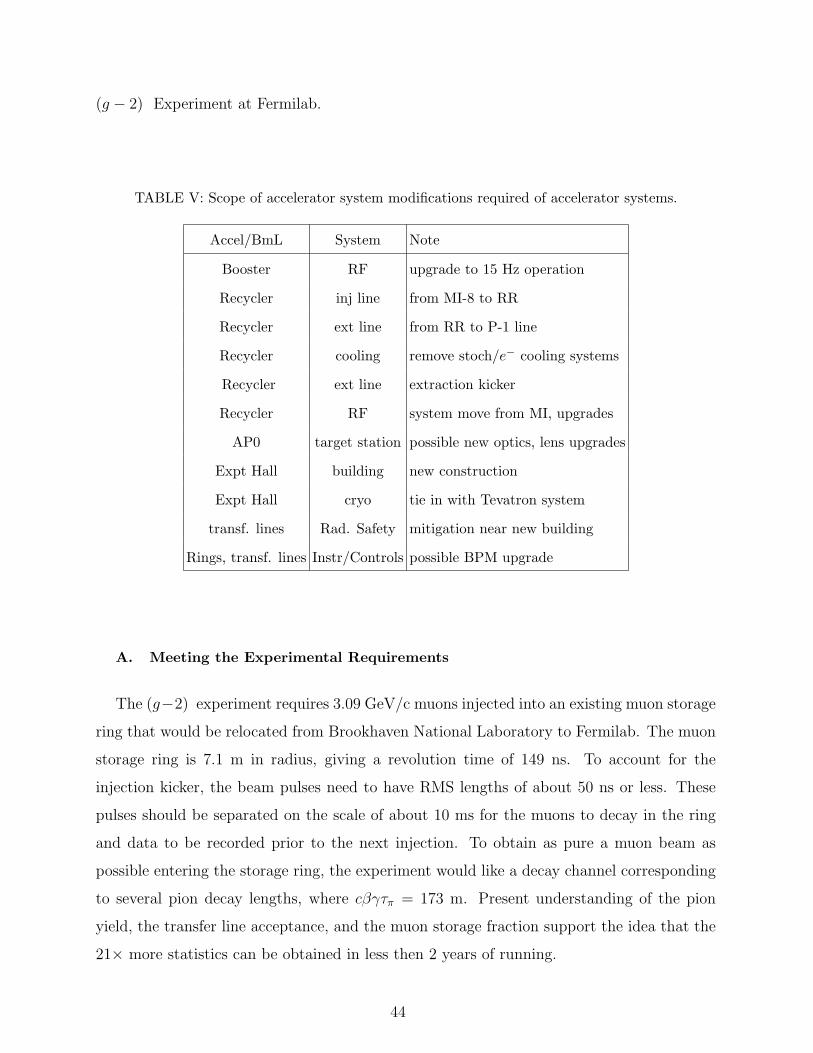
(g − 2) Experiment at Fermilab.
TABLE V: Scope of accelerator system modifications required of accelerator systems.
Accel/BmL System Note
Booster RF upgrade to 15 Hz operation
Recycler inj line from MI-8 to RR
Recycler ext line from RR to P-1 line
Recycler cooling remove stoch/e− cooling systems
Recycler ext line extraction kicker
Recycler RF system move from MI, upgrades
AP0 target station possible new optics, lens upgrades
Expt Hall building new construction
Expt Hall cryo tie in with Tevatron system
transf. lines Rad. Safety mitigation near new building
Rings, transf. lines Instr/Controls possible BPM upgrade
A. Meeting the Experimental Requirements
The (g−2) experiment requires 3.09 GeV/c muons injected into an existing muon storage
ring that would be relocated from Brookhaven National Laboratory to Fermilab. The muon
storage ring is 7.1 m in radius, giving a revolution time of 149 ns. To account for the
injection kicker, the beam pulses need to have RMS lengths of about 50 ns or less. These
pulses should be separated on the scale of about 10 ms for the muons to decay in the ring
and data to be recorded prior to the next injection. To obtain as pure a muon beam as
possible entering the storage ring, the experiment would like a decay channel corresponding
to several pion decay lengths, where cβγτπ = 173 m. Present understanding of the pion
yield, the transfer line acceptance, and the muon storage fraction support the idea that the
21× more statistics can be obtained in less then 2 years of running.
44
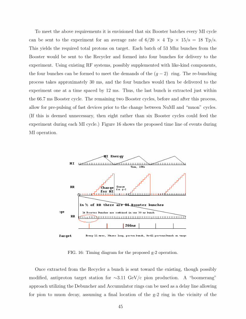
To meet the above requirements it is envisioned that six Booster batches every MI cycle
can be sent to the experiment for an average rate of 6/20 × 4 Tp × 15/s = 18 Tp/s.
This yields the required total protons on target. Each batch of 53 Mhz bunches from the
Booster would be sent to the Recycler and formed into four bunches for delivery to the
experiment. Using existing RF systems, possibly supplemented with like-kind components,
the four bunches can be formed to meet the demands of the (g − 2) ring. The re-bunching
process takes approximately 30 ms, and the four bunches would then be delivered to the
experiment one at a time spaced by 12 ms. Thus, the last bunch is extracted just within
the 66.7 ms Booster cycle. The remaining two Booster cycles, before and after this process,
allow for pre-pulsing of fast devices prior to the change between NuMI and “muon” cycles.
(If this is deemed unnecessary, then eight rather than six Booster cycles could feed the
experiment during each MI cycle.) Figure 16 shows the proposed time line of events during
MI operation.
FIG. 16: Timing diagram for the proposed g-2 operation.
Once extracted from the Recycler a bunch is sent toward the existing, though possibly
modified, antiproton target station for ∼3.11 GeV/c pion production. A “boomerang”
approach utilizing the Debuncher and Accumulator rings can be used as a delay line allowing
for pion to muon decay, assuming a final location of the g-2 ring in the vicinity of the
45

production target. A schematic of the beam line system is presented in Figure 17. The total
FIG. 17: Beam transport scheme for g-2 operation. Beam is prepared in the Recycler, exits via
the P1 line, passes through the Tevatron tunnel into the AP1 beam line, and to the AP0 target
area. (Blue curve.) Pions, decaying to muons, are transported from the target through the AP2
line, once around the “pbar” rings (Debuncher/Accumulator) and back toward the experimental
hall near AP0 via the AP3 beam line. (Thick red curve.)
length of the decay line would be ∼900 m. To obtain even further purity of the muon beam,
multiple revolutions in the Debuncher or Accumulator rings could be considered, perhaps as
an upgrade to the program. This upgrade would require the development of an appropriate
kicker system and is not included in this first design iteration. The 900 m decay length,
however, is already a large improvement over the original layout at BNL.
B. Bunch Formation
The major proton beam preparation will be performed in the Recycler ring. A broadband
RF system like that already installed in the Recycler would be used, except twice the voltage
may be required. The 2.5 MHz (max. Vrf = 60 kV) and 5 MHz (max. Vrf = 15 kV) RF
46

systems that presently reside in the MI would be relocated to the Recycler. Upgrades to
increase their maximum voltages by roughly 10-30% may be required. All of these upgrades
are assumed for the cost estimate.
As described in [59], the bunching scheme is to use a four period sawtooth wave form
across the Booster batch produced by the broadband RF system to break the batch into
four segments and rotate them in phase space sufficiently that they can be captured cleanly
in a linearized bucket provided by the resonant RF. Each of the four resulting bunches has
an RMS length of ∼50 ns. The first bunch is extracted immediately and the latter three
are extracted sequentially at half periods of the synchrotron oscillation. The beam loading
of the resonant cavities will be considerable, and further details need to be considered. It
is plausible to expect that a feedforward system can be developed without serious difficulty.
A combination of feedback with feed forward is potentially better yet, but feedforward will
be required with or without feedback. Figure 18 shows the resulting beam structure in the
FIG. 18: Resulting relative momentum spread (∆p/p) vs. time in seconds following injection into
the Recycler. After an initial phase using the broadband RF system, beam is captured into four
buckes. The beam rotates within the four buckets with period 12 ms and is extracted one-by-one
as the momentum spread reaches its peak (pulse length is at its shortest).
47

Recycler if the beam were not extracted. The plan would be to extract one pulse at a time,
every 12 ms, when the bunches are at their narrowest time extent (4σ widths of 38-58 ns).
The four bunches would be separated by roughly 400 ns center-to-center. For the sequence
shown, the RF systems require voltages of 4 kV (broadband), 80 kV (2.5 MHz), and 16 kV
(5.0 MHz). A longitudinal emittance of 0.07 eV-s per 53 MHz Booster bunch was assumed.
C. Beam Delivery and Transfer
Following the beam trajectory starting with extraction from the Booster, we see that the
proton beam needs to be injected into the Recycler from the MI-8 beam line at the MI-10
region of the Main Injector tunnel. This maneuver will be facilitated through the NOνA
project, which requires the same injection procedure. Once prepared with the RF systems
as described above, the beam will need to be extracted from the Recycler and injected into
the P1 beam line. The extraction location is at the MI-52 tunnel location, where the Main
Injector ties into this same beam line. (See Figure 17.) The P1 beam line is used to deliver
8 GeV antiprotons from the Accumulator into the Main Injector (and on into the Recycler)
in the reverse direction. During the g-2 operation, however, the Main Injector will contain
beam destined for NuMI and so this region will need to be modified in almost exactly the
same way as MI-10 to transport protons directly into the P1 line from the Recycler.
An appropriate kicker system will also be required for this region to extract one-by-
one the four proton bunches from the Recycler. The four bunches will be separated by
approximately 200 ns, so the kicker must rise in ∼180 ns and have a flat top of ∼50 ns. The
Recycler has a circumference seven times that of the Booster, and only one Booster batch
will be injected at a time. Thus, the last proton bunch of the four will be separated from
the first by about 8.6 µs or more. The kicker can then have a fall time on the order of 5 µs,
and must be pulsed 4 times separated by 10 ms within a Booster cycle. This operation is
repeated 6 times every 1.33 s MI cycle.
From the entrance of the P1 line through the Tevatron injection Lambertson (which is
kept off during this operation) the beam is directed through the P2 line (physically located
in the Tevatron tunnel) and into the AP1 line toward the AP0 target hall. Again, since this
system is run at 8 GeV for antiproton operations, no modifications are required for beam
transport in g-2 operations. After targeting, which is discussed in the next subsection,
48

3.1 GeV/c pions are collected into the AP2 line which is “retuned” to operate at 3.1 GeV/c
rather than today’s 8.89 GeV/c antiproton operation.
To obtain a long decay channel for the pions off the target, the beam is transported
through the AP2 line, into the Debuncher ring, and, through a new short transfer line,
into the AP3 line, and directed back toward AP0. (See Figure 17 again.) An alternative
option being considered is to transfer the beam from the Debuncher into the Accumulator
using existing lines; however, the present aperture restrictions in this simpler mode require
further study. As this will be the only use of these rings, kicker magnets will not be required
in this configuration, and the rings will be “partially powered” using only those magnet
strings required to perform the “boomerang.” Either corrector magnets or DC powered
trim magnets will be used in place of kickers to perform the injection/extraction between
the partially powered rings and associated beam lines. It is currently envisioned that the g-2
ring will be located on the surface near the AP0 service building as indicated in Figure 19.
The AP3 beam line will be modified to “punch through” the ceiling of the tunnel enclosure
FIG. 19: Proposed location of the new (g − 2) experimental hall (yellow).
and up into the g-2 ring.
As can be seen, little modifications are required of existing beam lines to perform the beam
transport all the way from the Booster to the g-2 ring. The end of the line and connection
49
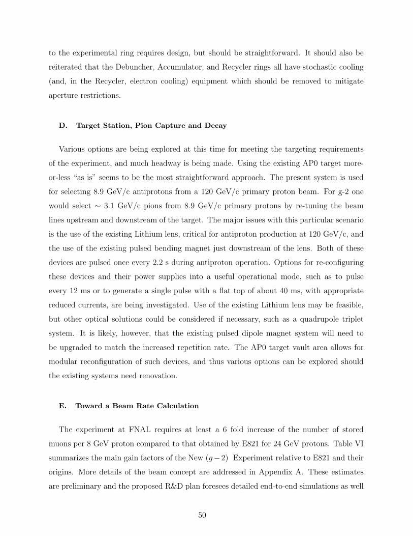
to the experimental ring requires design, but should be straightforward. It should also be
reiterated that the Debuncher, Accumulator, and Recycler rings all have stochastic cooling
(and, in the Recycler, electron cooling) equipment which should be removed to mitigate
aperture restrictions.
D. Target Station, Pion Capture and Decay
Various options are being explored at this time for meeting the targeting requirements
of the experiment, and much headway is being made. Using the existing AP0 target more-
or-less “as is” seems to be the most straightforward approach. The present system is used
for selecting 8.9 GeV/c antiprotons from a 120 GeV/c primary proton beam. For g-2 one
would select ∼ 3.1 GeV/c pions from 8.9 GeV/c primary protons by re-tuning the beam
lines upstream and downstream of the target. The major issues with this particular scenario
is the use of the existing Lithium lens, critical for antiproton production at 120 GeV/c, and
the use of the existing pulsed bending magnet just downstream of the lens. Both of these
devices are pulsed once every 2.2 s during antiproton operation. Options for re-configuring
these devices and their power supplies into a useful operational mode, such as to pulse
every 12 ms or to generate a single pulse with a flat top of about 40 ms, with appropriate
reduced currents, are being investigated. Use of the existing Lithium lens may be feasible,
but other optical solutions could be considered if necessary, such as a quadrupole triplet
system. It is likely, however, that the existing pulsed dipole magnet system will need to
be upgraded to match the increased repetition rate. The AP0 target vault area allows for
modular reconfiguration of such devices, and thus various options can be explored should
the existing systems need renovation.
E. Toward a Beam Rate Calculation
The experiment at FNAL requires at least a 6 fold increase of the number of stored
muons per 8 GeV proton compared to that obtained by E821 for 24 GeV protons. Table VI
summarizes the main gain factors of the New (g−2) Experiment relative to E821 and their
origins. More details of the beam concept are addressed in Appendix A. These estimates
are preliminary and the proposed R&D plan foresees detailed end-to-end simulations as well
50

as beam tests to corroborate these numbers. Additional improvements, due to a faster ring
injection kicker or tighter proton focusing on the production target, are under investigation.
Thus, the required gain factor of 6 can likely be exceeded, but we conservatively assume this
factor as a planning baseline for this proposal.
parameter BNL FNAL gain factor FNAL/BNL
Yπ pion/p into channel acceptance ≈ 2.7E-5 ≈ 1.1E-5 0.4
L decay channel length 88 m 900 m 2
decay angle in lab system 3.8 ± 0.5 mr forward 3
δpπ/pπ pion momentum band ±0.5% ±2% 1.33
FODO lattice spacing 6.2 m 3.25 m 1.8
inflector closed end open end 2
total 11.5
TABLE VI: Parameters for E821 and the New (g − 2) Experiment beamline and their relative
effect on the stored muons per proton fraction. Pion yield Yπ given for pion momentum bin pπ=
3.11 GeV/c ± 0.5%.
F. Experimental Facility
A first pass look at an experimental building was performed at Fermilab.[60] The building
would be approximately 80 ft × 80 ft and includes a full-span 40 ton bridge crane. Other
details of the cost exercise may be found in [60]. The building is large enough to enclose the
g-2 ring as well as associated electronics and counting room. A schematic of the building
location and adjacent parking area are found in Figure 20.
The cryogenic needs of the experiment can be met by the Tevatron accelerator cryogenics
system with some modifications and additional transfer line work. The Tevatron is located
only about 50 ft away from the AP0 service building, and is expected to be in 80K standby
mode during the time span of the experiment. Additionally, it is assumed that the Tevatron
F2 magnet string is allowed to be warmed up to room temperature during this time, freeing
up the refrigeration system at F2 to be used for g-2. A cost estimate of the required
modifications has been performed and documented.[61]
51
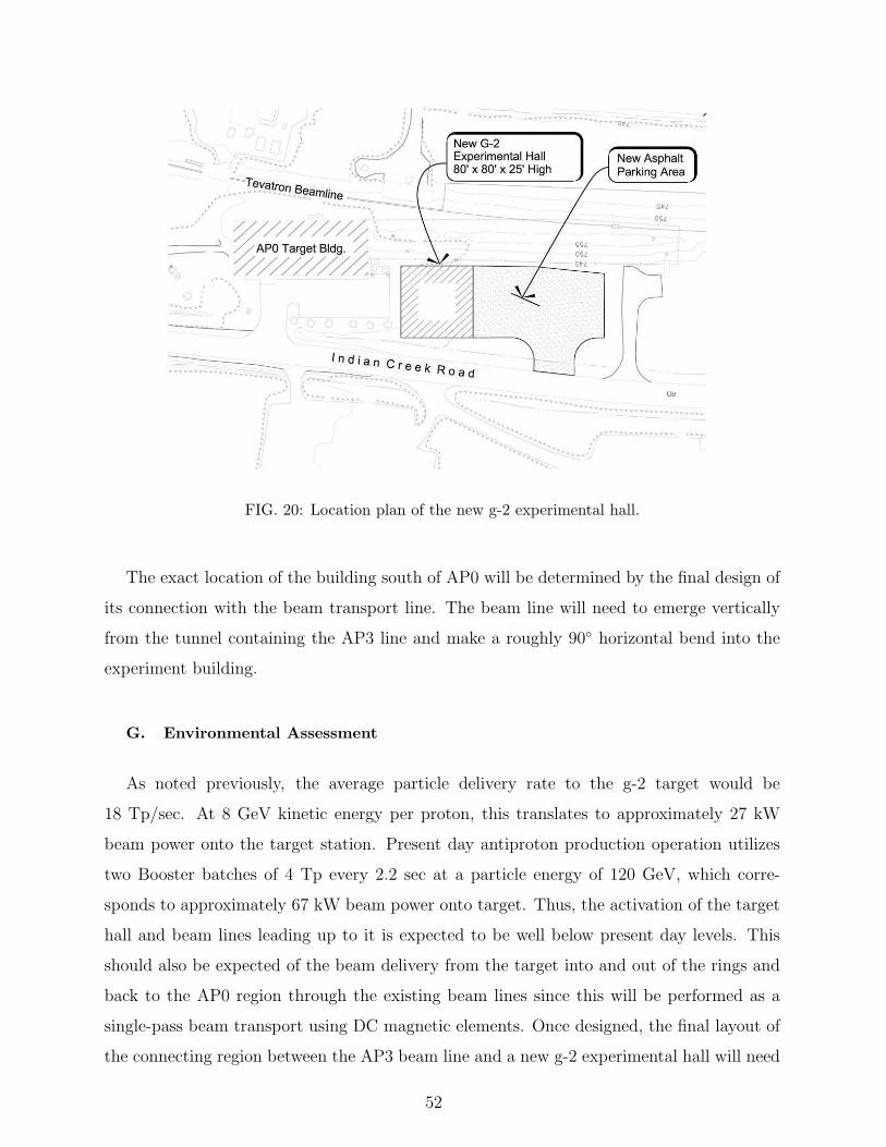
!
FIG. 20: Location plan of the new g-2 experimental hall.
The exact location of the building south of AP0 will be determined by the final design of
its connection with the beam transport line. The beam line will need to emerge vertically
from the tunnel containing the AP3 line and make a roughly 90 horizontal bend into the
experiment building.
G. Environmental Assessment
As noted previously, the average particle delivery rate to the g-2 target would be
18 Tp/sec. At 8 GeV kinetic energy per proton, this translates to approximately 27 kW
beam power onto the target station. Present day antiproton production operation utilizes
two Booster batches of 4 Tp every 2.2 sec at a particle energy of 120 GeV, which corre-
sponds to approximately 67 kW beam power onto target. Thus, the activation of the target
hall and beam lines leading up to it is expected to be well below present day levels. This
should also be expected of the beam delivery from the target into and out of the rings and
back to the AP0 region through the existing beam lines since this will be performed as a
single-pass beam transport using DC magnetic elements. Once designed, the final layout of
the connecting region between the AP3 beam line and a new g-2 experimental hall will need
52

to be assessed for appropriate shielding. While further work will be needed to validate the
environmental impact of the new use of these facilities for g-2, as well as for the experimental
building itself, this is seen as a straightforward effort.
H. Opening the Inflector Ends
The original superconducting inflector design for BNL E821 included two options for
the ends: open or closed, see Fig. 21. Both versions were built in 0.5 m long prototype
form, but only the closed-end version was built at full scale (1.7 m length) and used in the
experiment [62, 63]. The closed inflector was selected because of its simpler construction
and was thought to be more stable against Lorentz forces. Further, the closed-end inflector
has a smaller fringe field that could be more easily shielded from the storage ring field seen
by the muons. On the downside, beam transport studies show that multiple scattering and
energy loss in the closed end reduce the transmission of muons that store in the ring by a
factor of 2.
The stability of the open-ended coil configuration was demonstrated at full current in a
1.5 T external magnetic field. Based on our measurements [63], the added leakage field from
the open end can be excluded from the storage region by a passive superconducting sheet.
A factor of 2 increase in muon flux is expected from opening the ends. Much of the
investment in engineering for this device has already been made and custom tooling necessary
to construct the magnet exists. The inflector is discussed in detail in an appendix.
I. Accelerator R&D
As of this writing the major items requiring attention include:
• Targeting and Pion Flux: The target optics needs to be verified and/or re-designed if
necessary, including the possible use of the lithium lens, and the final target material
chosen or verified. The possible use of the existing pulsed dipole magnet in the target
hall needs to be addressed as well and options identified should this magnet not meet
specifications. Headway is being made quickly on understanding the expected pion flux
from targeting of 8 GeV kinetic energy protons. The associated production acceptance
53
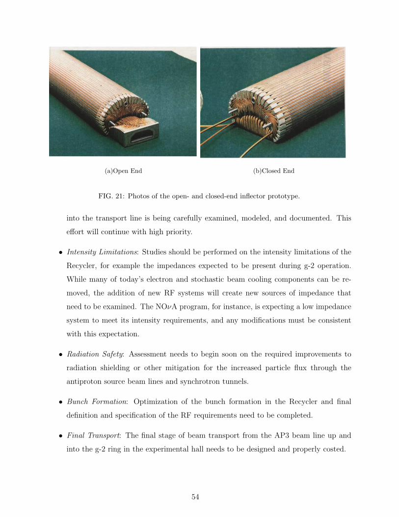
(a)Open End (b)Closed End
FIG. 21: Photos of the open- and closed-end inflector prototype.
into the transport line is being carefully examined, modeled, and documented. This
effort will continue with high priority.
• Intensity Limitations: Studies should be performed on the intensity limitations of the
Recycler, for example the impedances expected to be present during g-2 operation.
While many of today’s electron and stochastic beam cooling components can be re-
moved, the addition of new RF systems will create new sources of impedance that
need to be examined. The NOνA program, for instance, is expecting a low impedance
system to meet its intensity requirements, and any modifications must be consistent
with this expectation.
• Radiation Safety: Assessment needs to begin soon on the required improvements to
radiation shielding or other mitigation for the increased particle flux through the
antiproton source beam lines and synchrotron tunnels.
• Bunch Formation: Optimization of the bunch formation in the Recycler and final
definition and specification of the RF requirements need to be completed.
• Final Transport: The final stage of beam transport from the AP3 beam line up and
into the g-2 ring in the experimental hall needs to be designed and properly costed.
54
J. Muon Storage Ring Magnet
The muon storage ring [64] is a superferric “C”-shaped magnet, 7.112 m in central orbit
radius, and open on the inside to permit the decay electrons to curl inward to the detectors
(Fig. 22). A 5 V power supply drives a 5177 A current in the three NbTi/Cu superconducting
coils. Feedback to the power supply from the NMR field measurements maintains the field
stability to several ppm. The field is designed to be vertical and uniform at a central value
of 1.4513 T. High-quality steel, having a maximum of 0.08 percent carbon, is used in the
yoke. Low-carbon steel is used for the poles primarily because the fabrication process of
continuous cast steel greatly minimizes impurities such as inclusions of ferritic or other
extraneous material and air bubbles. An air gap between the yoke and the higher quality
pole pieces decouples the field in the storage region from non-uniformities in the yoke. Steel
wedge shims are placed in the air gap. Eighty low-current surface correction coils go around
the ring on the pole piece faces for active trimming of the field. The opening between the
pole faces is 180 mm and the storage region is 90 mm in diameter. A vertical cross section of
the storage ring illustrating some of these key features is shown in Fig. 23. Selected storage
ring parameters are listed in Table VII.
Attaining high field uniformity requires a series of passive shimming adjustments, starting
far from and then proceeding towards the storage region. First the twelve upper- and lower-
yoke adjustment plates are shimmed by placing precision spacers between them and the yoke
steel, modifying the air gap. Next the 1000 wedge shims in the yoke pole-piece air gap are
adjusted. With a wedge angle of 50 mrad, adjusting the wedge position radially by 1 mm
changes the thickness of iron at the center of the storage aperture by 50 µm. The wedge
angle is set to compensate the quadrupole component, and radial adjustments of the wedge
and other changes to the air gap are used to shim the local dipole field. The local sextupole
field is minimized by changing the thickness of the 144 edge shims, which sit on the inner
and outer radial edges of the pole faces. Higher moments, largely uniform around the ring,
are reduced by adjusting the 240 surface-correction coils, which run azimuthally for 360
degrees along the surface of the pole faces. They are controlled through 16 programmable
current elements. With adjustments made, the azimuthally averaged magnetic field in the
storage volume had a uniformity of ' 1 ppm during data-taking runs.
The main temporal variation in the magnetic field uniformity is associated with radial
55

TABLE VII: Selected muon storage ring parameters.
Parameter Value
Nominal magnetic field 1.4513 T
Nominal current 5200 A
Equilibrium orbit radius 7.112 m
Muon storage region diameter 90 mm
Magnet gap 180 mm
Stored energy 6 MJ
field changes from seasonal and diurnal drift in the iron temperature. Because of the “C”
magnet geometry, increasing (or decreasing) the outside yoke temperature can tilt the pole
faces together (or apart), creating a radial gradient. The yoke steel was insulated prior to
the R98 run with 150 mm of fiberglass to reduce the magnetic-field variation with external
temperature changes to a negligible level.
K. Relocating the Storage Ring to FNAL
Moving the experiment to FNAL entails the disassembly and shipping of the storage ring
along with all of its various subsystems. The subsystems can be disassembled and shipped
conventionally, including power supplies and control systems, cryo elements and quench
protection, vacuum chambers and pumping stations, electrostatic quadrupoles, shimming
devices and NMR systems, and magnetic kickers. The steel plates that form the yoke, see
Fig. 23, are constructed in 12 sectors each covering 30 degrees in azimuth. The plates can
be unbolted and transported with a total shipping weight of 680 metric tons.
The main complication in moving the storage ring involves transporting the cryostats that
contain the superconducting coils. The three cryostats, shown in cross-section in Fig. 23,
are monolithic rings approximately 14 m in diameter. The outer cryostat holds a 48-turn
coil separated into two blocks of 24 turns to allow the muons to enter through the space
between. Two inner cryostats hold 24-turn coils connected in series to the outer coil with
the current flow reversed. Given the large diameter of the coils, shipping overland is not
possible. Moving the coils requires airlifting them from Brookhaven to a barge off the Long
56

FIG. 22: A 3D engineering rendition of the E821 muon storage ring. Muons enter the back of
the storage ring through a field-free channel at approximately 10 o’clock in the figure. The three
kicker modulators at approximately 2 o’clock provide the short current pulse, which gives the
muon bunch a transverse 10 mrad kick. The regularly spaced boxes on rails represent the electron
detector systems.
Island Sound, shipping them through the St. Lawrence Seaway, and into the Great Lakes.
From Lake Michigan, the barge can travel via the Calumet SAG channel to a point near
Lemont, IL that minimizes the distance to Fermilab. From there, the coils can be airlifted a
second time to the laboratory. The total shipping cost for the water transport is estimated
at $700K.
One advantage of the proposed route, is the proximity of major expressways between the
barge and the laboratories. On Long Island, the William Floyd Parkway, and in Illinois,
I-355 to I-88, provide flight paths that avoid air space over residential or commercial areas.
Erickson Air-Crane has been contacted for an initial cost estimate and consultation on
feasibility. The company is an international specialist in heavy-lift applications, and their
S-64 aircrane has a 25,000 lb load capacity, which is enough to transfer the heaviest of the
57

Shim plateThrough bolt
Iron yoke
slotOuter coil
Spacer Plates
1570 mm
544 mm
Inner upper coil
Poles
Inner lower coil
To ring center
Muon beam
Upper push−rod
1394 mm
360 mm
FIG. 23: Cross sectional view of the “C” magnet.
coils along with its lifting rig. The cost for the entire air crane operation at both ends of
the barge voyage was quoted at $380K.
For the purpose of this proposal, it is assumed that the coils will be transferred from BNL
to FNAL. While this provides an upper limit to the overall cost estimate of approximately
$1.1M (without contingency) to transfer the coils, the price to re-fabricate the coils and
cryostats at Fermilab needs to be explored. Given that the price to construct the cryostats
and wind the coils originally totaled $2.3M in 1990 dollars, it is unlikely to be advantageous
to consider rebuilding them. There is also a secondary advantage in utilizing a barge in that
the steel from the magnet yoke can be delivered to and from the same barge for a significant
savings compared to shipping overland.
58
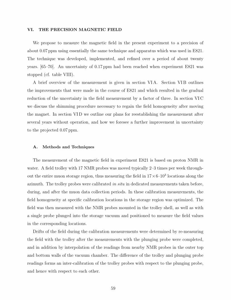
VI. THE PRECISION MAGNETIC FIELD
We propose to measure the magnetic field in the present experiment to a precision of
about 0.07 ppm using essentially the same technique and apparatus which was used in E821.
The technique was developed, implemented, and refined over a period of about twenty
years. [65–70]. An uncertainty of 0.17 ppm had been reached when experiment E821 was
stopped (cf. table VIII).
A brief overview of the measurement is given in section VIA. Section VIB outlines
the improvements that were made in the course of E821 and which resulted in the gradual
reduction of the uncertainty in the field measurement by a factor of three. In section VIC
we discuss the shimming procedure necessary to regain the field homogeneity after moving
the magnet. In section VID we outline our plans for reestablishing the measurement after
several years without operation, and how we foresee a further improvement in uncertainty
to the projected 0.07 ppm.
A. Methods and Techniques
The measurement of the magnetic field in experiment E821 is based on proton NMR in
water. A field trolley with 17 NMR probes was moved typically 2–3 times per week through-
out the entire muon storage region, thus measuring the field in 17×6 ·103 locations along the
azimuth. The trolley probes were calibrated in situ in dedicated measurements taken before,
during, and after the muon data collection periods. In these calibration measurements, the
field homogeneity at specific calibration locations in the storage region was optimized. The
field was then measured with the NMR probes mounted in the trolley shell, as well as with
a single probe plunged into the storage vacuum and positioned to measure the field values
in the corresponding locations.
Drifts of the field during the calibration measurements were determined by re-measuring
the field with the trolley after the measurements with the plunging probe were completed,
and in addition by interpolation of the readings from nearby NMR probes in the outer top
and bottom walls of the vacuum chamber. The difference of the trolley and plunging probe
readings forms an inter-calibration of the trolley probes with respect to the plunging probe,
and hence with respect to each other.
59

The plunging probe, as well as a subset of the trolley probes, were calibrated with respect
to a standard probe [74] with a 1 cm diameter spherical H2O sample in a similar sequence of
measurements in the storage region, which was opened to air for that purpose. The standard
probe is the same as the one used in the muonium measurements that determine the ratio
λ of muon to proton magnetic moments [13].
The NMR clock and the clock that measured the muon spin precession period were phase-
locked to the same LORAN-C [75] signal. Systematic effects include the instrument response
and were extensively studied. The leading uncertainties in the calibration procedure resulted
from the residual inhomogeneity of the field at the calibration locations, and from position
uncertainties in the active volumes of the NMR probes.
The ring magnet design [71], the inflector design [72], and extensive shimming contributed
to the overall uniformity of the field throughout the storage ring. Figure 24 shows one of the
magnetic field measurements with the center NMR probe in the trolley for E821’s final data
collection period in the year 2001. A uniformity of ±100 ppm in the center of the storage
region was achieved for both field polarities and for the full azimuthal range, in particular
also in the region where the inflector magnet is located.
Figure 25 shows a two-dimensional multipole expansion of the azimuthal average of the
field in the muon storage region from a typical trolley measurement in 2001. Since the aver-
age field is uniform to within 1.5 ppm over the storage aperture, the field integral encountered
by the (analyzed) muons is rather insensitive to the profile and the precise location of the
beam, which was determined to within a millimeter in both coordinates.
The measurements with the field trolley were used to relate the readings of about 150
(out of 370) NMR fixed probes in the outer top and bottom walls of the storage vacuum
chamber to the field values in the beam region. The fixed NMR probes were read out
continually. Their readings were used to interpolate the field during data collection periods,
when the field trolley was parked in a garage inside of the vacuum chamber. The garage is
located just outside the beam region. The uncertainty in this interpolation was estimated
from redundant measurements with the field trolley within the same magnet-on period.
The field change induced by eddy currents from the pulsed kickers was measured for
a prototype chamber with an optical magnetometer [73]. Time-varying stray fields from
the accelerator were measured in situ with the NMR system [66, 67] and found to con-
tribute negligible uncertainty. Another small uncertainty comes from the off-vertical field
60
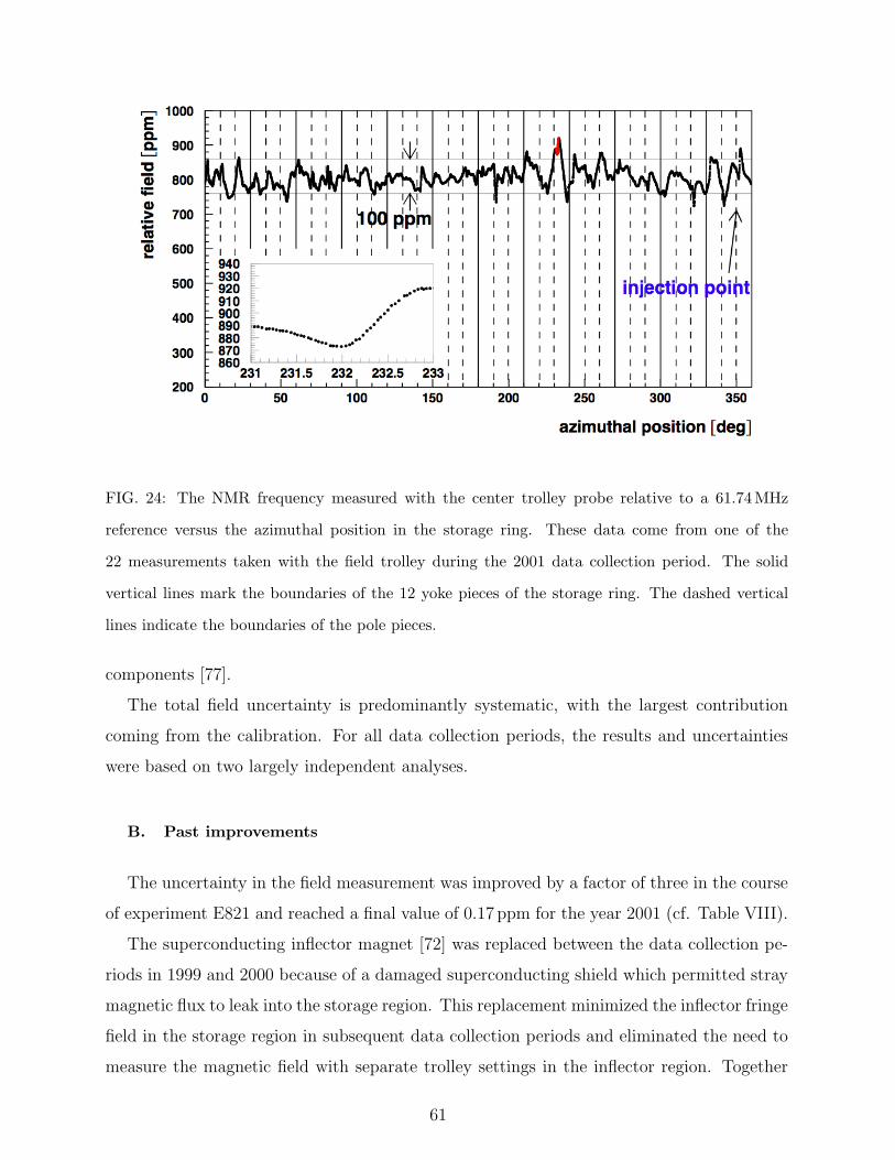
FIG. 24: The NMR frequency measured with the center trolley probe relative to a 61.74MHz
reference versus the azimuthal position in the storage ring. These data come from one of the
22 measurements taken with the field trolley during the 2001 data collection period. The solid
vertical lines mark the boundaries of the 12 yoke pieces of the storage ring. The dashed vertical
lines indicate the boundaries of the pole pieces.
components [77].
The total field uncertainty is predominantly systematic, with the largest contribution
coming from the calibration. For all data collection periods, the results and uncertainties
were based on two largely independent analyses.
B. Past improvements
The uncertainty in the field measurement was improved by a factor of three in the course
of experiment E821 and reached a final value of 0.17 ppm for the year 2001 (cf. Table VIII).
The superconducting inflector magnet [72] was replaced between the data collection pe-
riods in 1999 and 2000 because of a damaged superconducting shield which permitted stray
magnetic flux to leak into the storage region. This replacement minimized the inflector fringe
field in the storage region in subsequent data collection periods and eliminated the need to
measure the magnetic field with separate trolley settings in the inflector region. Together
61
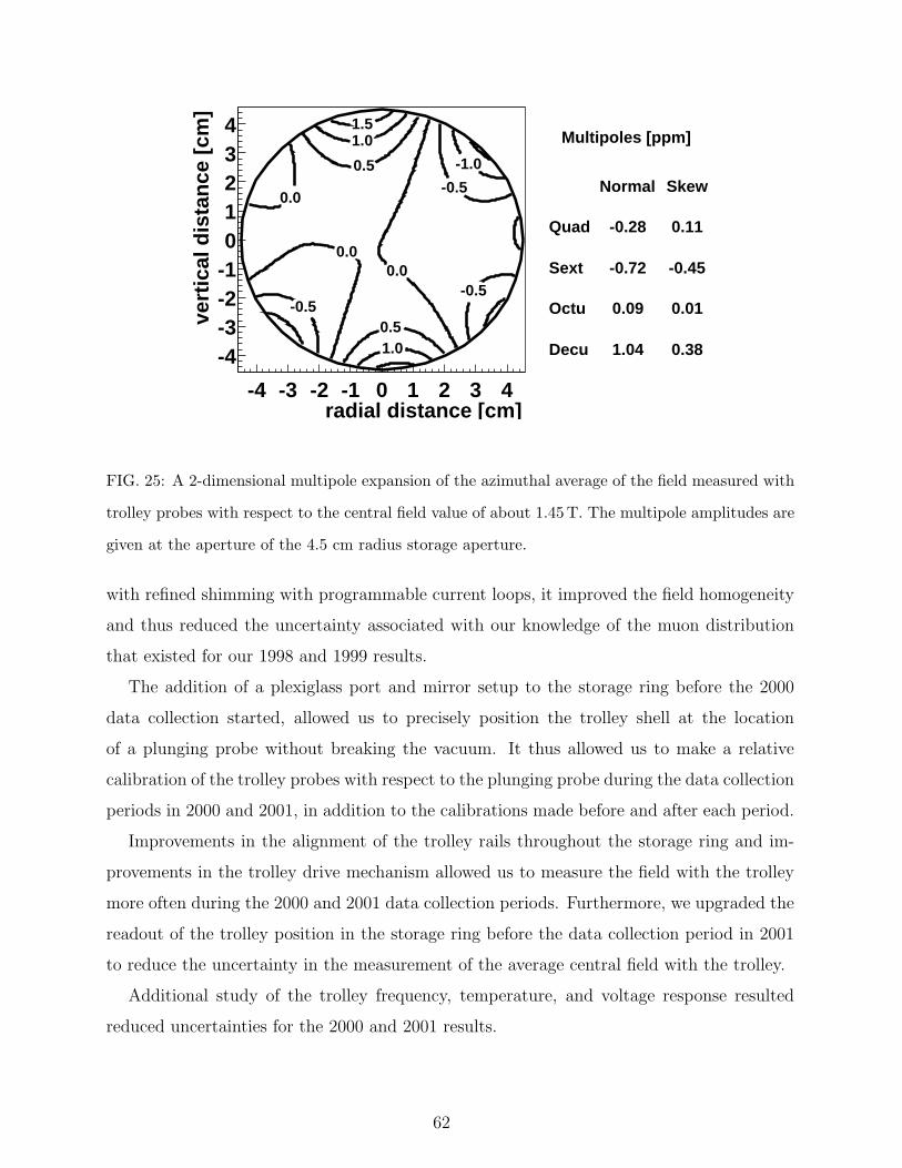
Multipoles [ppm]
Normal Skew
Quad -0.28 0.11
Sext -0.72 -0.45
Octu 0.09 0.01
Decu 1.04 0.38
radial distance [cm]-4 -3 -2 -1 0 1 2 3 4
vert
ical
dis
tan
ce [
cm]
-4-3-2-101234
-1.0
-0.5
-0.5-0.5
0.00.0
0.0
0.5
1.01.5
0.51.0
FIG. 25: A 2-dimensional multipole expansion of the azimuthal average of the field measured with
trolley probes with respect to the central field value of about 1.45T. The multipole amplitudes are
given at the aperture of the 4.5 cm radius storage aperture.
with refined shimming with programmable current loops, it improved the field homogeneity
and thus reduced the uncertainty associated with our knowledge of the muon distribution
that existed for our 1998 and 1999 results.
The addition of a plexiglass port and mirror setup to the storage ring before the 2000
data collection started, allowed us to precisely position the trolley shell at the location
of a plunging probe without breaking the vacuum. It thus allowed us to make a relative
calibration of the trolley probes with respect to the plunging probe during the data collection
periods in 2000 and 2001, in addition to the calibrations made before and after each period.
Improvements in the alignment of the trolley rails throughout the storage ring and im-
provements in the trolley drive mechanism allowed us to measure the field with the trolley
more often during the 2000 and 2001 data collection periods. Furthermore, we upgraded the
readout of the trolley position in the storage ring before the data collection period in 2001
to reduce the uncertainty in the measurement of the average central field with the trolley.
Additional study of the trolley frequency, temperature, and voltage response resulted
reduced uncertainties for the 2000 and 2001 results.
62

TABLE VIII: Systematic uncertainties in the measurement of the magnetic field for experiment
E821 (1998–2001) and our projections for a future effort based on known techniques and existing
equipment. The uncertainty ”Others” groups uncertainties caused by higher multipoles, the trolley
frequency, temperature, and voltage response, eddy currents from the kickers, and time-varying
stray fields.
Source of errors Size [ppm]
1998 1999 2000 2001 future
Absolute calibration of standard probe 0.05 0.05 0.05 0.05 0.05
Calibration of trolley probe 0.3 0.20 0.15 0.09 0.06
Trolley measurements of B0 0.1 0.10 0.10 0.05 0.02
Interpolation with fixed probes 0.3 0.15 0.10 0.07 0.06
Inflector fringe field 0.2 0.20 - - -
Uncertainty from muon distribution 0.1 0.12 0.03 0.03 0.02
Others 0.15 0.10 0.10 0.05
Total systematic error on ωp 0.5 0.4 0.24 0.17 0.11
C. Shimming the Storage Ring Magnetic Field
The success of the experiment requires that the magnetic field be shimmed to a uniformity
of ≈ 1 ppm averaged over the storage volume. This was essentially achieved by BNL E821.
A more stringent requirement of the new experiment is that the field be measured to a
precision of less than about 0.1 ppm. Improvements in field uniformity over those achieved
in E821 will help to reach this more challenging goal.
The magnet was assembled as a kit at BNL, and would be assembled in a similar fashion
at FNAL. The magnet is made of 12 C-shaped iron yoke sectors, each in turn composed
of precision engineered, low carbon steel plates. Variations in the yoke plate thicknesses of
the order of 200 µm, cause similar variations in the 20 cm air gap, leading to variations
in the dipole field of 1000 ppm around the storage ring. Changes in the yoke permeability
from sector to sector also lead to changes in the dipole field, as do tilts, gaps, and other
imperfections.
Practical mechanical tolerances thus inevitably lead to variations of the magnetic field of
63

a thousand ppm. It is therefore unavoidable that reassembling the storage ring at Fermilab
will lead to the loss of field homogeneity realized at Brookhaven.
Reattaining high field uniformity requires a series of shimming steps, well established by
E821, from coarse to fine adjustments, and from mechanical to electrical techniques.
First the 12 upper and lower-yoke adjustment plates are shimmed by placing precision
spacers between them and the yoke steel, modifying the air gap. The precision pole pieces
are adjusted so that the surfaces of adjacent pole pieces are matched to ± 10 µm. The
angles of the poles are measured to ± 50µrad, and adjusted so the pole faces are horizontal
when the magnet is powered.
Next, the precision pole pieces are attached to each yoke sector, separated by a 1 cm
air gap. In the air gap are inserted a total of 864 adjustable iron wedges. The wedges
were machined with an angle of 50mrad to compensate for the normal quadrupole moment
expected from the C-magnet design. Moving a single wedge radially by ±3mm changes
the air gap by ±150µm, changing the dipole field locally by ±300 ppm (with higher order
moments essentially unchanged). Finer movements allow correspondingly finer adjustments
of the dipole field.
The air gap also contains dipole corrections coils (DCCs) which allows the dipole field
over a pole to be adjusted by ± 200 ppm. The currents in these 72 DCCs were static in
E821, but active feedback is possible.
With these tools, the variation of the dipole field around the ring can be reduced to
acceptable levels.
Higher order moments of the field are reduced by shimming elements placed between
the pole faces and the storage volume. These include 5 cm wide iron shims placed on the
inner and outer radius of each pole. The edge shim thicknesses are adjusted to minimize
the normal sextupole, and skew quadrupole and sextupole. It would be prudent to produce
new edge shims, though it is possible none would be required.
Another tool for reducing higher order moments are the surface correction coils (SCCs).
These are a set of 2 × 120 coils, 360 in azimuth on PCBs, 2.5 mm apart, carrying ± 1A.
The currents through the coils are set individually to reduce the average of the normal
quadrupole and other moments over the ring. With these tools, a uniformity of ≈1 ppm
should be achievable.
It is important to mention that maintaining this homogeneity requires that the magnet
64
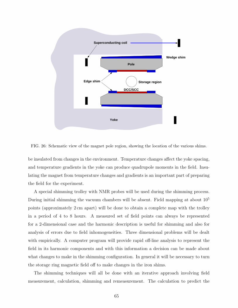
Wedge shim
Pole
Yoke
Storage region
Superconducting coil
DCC/SCC
Edge shim
FIG. 26: Schematic view of the magnet pole region, showing the location of the various shims.
be insulated from changes in the environment. Temperature changes affect the yoke spacing,
and temperature gradients in the yoke can produce quadrupole moments in the field. Insu-
lating the magnet from temperature changes and gradients is an important part of preparing
the field for the experiment.
A special shimming trolley with NMR probes will be used during the shimming process.
During initial shimming the vacuum chambers will be absent. Field mapping at about 105
points (approximately 2 cm apart) will be done to obtain a complete map with the trolley
in a period of 4 to 8 hours. A measured set of field points can always be represented
for a 2-dimensional case and the harmonic description is useful for shimming and also for
analysis of errors due to field inhomogeneities. Three dimensional problems will be dealt
with empirically. A computer program will provide rapid off-line analysis to represent the
field in its harmonic components and with this information a decision can be made about
what changes to make in the shimming configuration. In general it will be necessary to turn
the storage ring magnetic field off to make changes in the iron shims.
The shimming techniques will all be done with an iterative approach involving field
measurement, calculation, shimming and remeasurement. The calculation to predict the
65

shimming required to improve the field will depend on the particular shimming technique
being employed and on the character of the inhomogeneity.
We can anticipate at least 6 months or more will be required (once the magnet has been
reassembled and powered) to shim the magnet without the vacuum chambers in place. This
time would be used to adjust the pole face positions and tilts, to adjust the wedges and
DCCs, make fine adjustments with the thin iron shims, and to make any changes to the
edge shims. Note that some sort of mechanism for moving the shimming trolley around the
ring will be necessary, as well as a means of determining its azimuthal position.
D. Further Improvements
The methods and techniques used in E821 are not fully exhausted; to reach a precision
of 0.11 ppm, as detailed in Table VIII, only modest refinements are necessary. To reach the
projected 0.07 ppm, no single approach suffices, and several systematic error sources need
to be addressed simultaneously.
Our efforts to improve the existing apparatus and techniques would be focussed on the
following items.
• in situ measurement of the field change from kicker eddy currents [73].
• Extensive measurements with the magnetic field trolley, aiming in particular to better
resolve the position of the active NMR volumes inside the trolley shell and to map
out the response functions to the level where corrections can be applied, rather than
limits be set.
• More frequent measurements of the magnetic field in the storage ring during beam
periods (following mechanical maintenance on the trolley drive and garage).
• Repair and retuning of a number of the fixed NMR probes to improve the sampling
of the storage ring.
• Replacement of the power supplies for the surface correction coils to eliminate the
occasional data loss caused by oscillating outputs.
• Refinement of the analysis techniques to reduce trolley position uncertainties in the
storage ring.
66

• Temperature control of the environment of the storage ring magnet.
• Additional shimming of the storage ring once the homogeneity of the E821 field has
been reestablished at FNAL.
• Use thin (25-100µm) iron shims on the pole faces to further reduce azimuthal variations
in the dipole field, which primarily couples to uncertainty in trolley position.
• Replacement of outdated computing and readout infrastructure.
• Replacement of the LORAN-C time reference by GPS-based system, if necessary.
Better knowledge of the muon beam distribution, required by the anomalous precession
measurement, would also benefit the measurement of the average magnetic field.
Further improvements down to the final goal of 0.07 ppm require significant R&D. Several
aspects of the measurement need to be addressed simultaneously, as no single improvement
suffices to reach this level of precision. Development of new experimental techniques and
equipment include
• Replacement of the water-based absolute calibration probe by a 3He based system;
• Re-positioning of the fixed probes;
• Upgrade of the NMR trolley drive system;
• Upgrade of the plunging probe drive; and
• Re-machining of the precision poles.
Continued development of an independent helium-3 based standard probe [78], would benefit
the field measurement, however, the projected uncertainty of 0.07 ppm does not rely on it.
About half of the fixed probes could not be used effectively, due to their proximity to the
joints in the precision pole pieces and yoke and the resulting field inhomogeneity. For those
used, an empirical importance (weight factor) was assigned, depending on its location. By
increasing the usable number and effectiveness of the fixed probes, the field tracking uncer-
tainty in-between trolley runs can be further improved. An extensive simulation program,
including a detailed field description that includes the effect of the magnet imperfections
67

and the specifics of the fixed probes, will be needed to find optimal positions. Modification
of the vacuum chambers will have to be taken into account.
Tracking of higher multipoles, and thus the interpolation uncertainty, would greatly ben-
efit from the placement of probes in the midplane of the storage volume, rather than just
above and below it. Because of the geometry of the vacuum chambers this would imply
placement in vacuo and as close as possible to the horizontal quadrupole plates. At the
inner radius of the ring, these probes could interfere with the placement of the calorimeters
and other equipment. A probe that can operate in this environment, including a mounting
and cabling scheme, has to be developed and the vacuum chambers will have to be adapted.
An increase of the speed with which the trolley moves though the ring would allow
for more (frequent) measurements in the storage volume. It would simultaneously address
the reduction of several sources of uncertainty, such as the trolley temperature and field
interpolation. It requires the redesign of the trolley drive, together with an improvement in
the alignment of the trolley rails. Besides to an increase in trolley speed, the latter will also
lead to a reduction of the trolley position uncertainty, which coupled to the azimuthal field
inhomogeneity affects the uncertainty in the averaged field B0.
The relative calibration of the trolley probes can be improved by operating the plunging
probe more frequently, perhaps even during each trolley run. This would require the de-
velopment of a faster, more powerful plunging probe drive, which has to operate close the
precision field, without affecting it at a significant level.
Finally, with the advent of more powerful magnet design tools and computer-aided ma-
chining tools, it should be investigated whether the precision poles should be re-shaped to
eliminate the need and limitations of the edge shims.
The successful completion of these improvements are expected to suffice to reach the
projected goal 0.07 ppm, together with the refinements mentioned before. We do note,
however, that the improvement relies significantly on measurement of the field change from
kicker eddy currents and the absence of field perturbations caused by the redesigned (open)
inflector magnet. Neither of these have been demonstrated to a sufficient level at this time.
We are confident that a field knowledge to a precision of 0.11 ppm can be reached using the
existing experience in the field group. The present hardware has the potential to reach that
level with the moderate aforementioned repairs and upgrades. A further reduction down to
0.07 ppm appears reachable with the successful completion of a multi-facetted R&D program
68

aimed at reducing several systematic uncertainties simultaneously.
VII. ωA MEASUREMENT
A. Overview
The measurement of ωa is made by recording the arrival times and energies of decay
positrons in a suite of 24 electromagnetic calorimeters. A position-sensitive straw chamber
is placed upstream of each calorimeter to record impact positions and to provide horizontal
and vertical distributions, which are important for stored beam diagnostics. Coincident
events, which penetrate two or three adjacent calorimeter stations, serve as “lost muon” de-
tectors. Additional straw chambers, placed upstream of the calorimeters, inside the vacuum,
provide detailed beam dynamic information and serve as the basis for a parasitic electric
dipole moment measurement. This chapter describes the systems we will use for the ωa
measurement, which are largely based on the experience obtained in E821.
For planning purposes, we assume that the expected rates in the new experiment will
slightly exceed those of E821. The empirical argument to gauge the increase follows. The
total E821 statistics of 8.5 × 10⁹ events was accumulated in 2.5 × 10⁷ storage ring fills.
Allowing for efficiency factors consistent with those described in Table IV, E821 ran for
0.8 × 10⁷ seconds using ≈ 1.5 × 10²⁰ protons on target (POT). In this summary of E821,
commissioning time is excluded. At FNAL, the storage ring fill frequency will be greater by
a factor of 4 and the requested data-taking period is longer by a factor of nearly 4. Thus,
the number of storage ring fills in the final sample will be greater by a factor of ∼ 15;
the 21 times increase in statistics then roughly implies that the experiment will be carried
out at a rate ∼ 1.5 times higher (we are rounding here). Under planned beam delivery
scenarios, it could rise by as much as a factor of 3. Consequently, the detectors, electronics
and DAQ, will be designed to accept sustained rates per fill up to 3 times as high as BNL
E821. The rate comparison is important because it guides upgraded or new systems. First,
the instantaneous rate near fit start time determines the pileup fraction, which is a critical
systematic uncertainty. Second, the total data flow determines the details of the electronics
and DAQ systems, their data transfer rates and the total data storage required.
Higher data rates lead to the conclusion that segmented electromagnetic calorimeters
69

are required to reduce the pileup fraction per channel. Additionally, the position sensitive
detectors must have higher segmentation. We describe a design below, which satisfies these
demands.
New waveform digitizers (WFDs) will be used to continuously digitize the analog signals
from the calorimeter segments during each fill period. These data will flow to dedicated
pre-frontend processors upstream of the frontend data acquisition modules where they will
be packaged into event streams of derived databanks for the so-called T -method and Q-
method analyses (see below). The collaboration has experience in building and running
WFDs. After E821, we built more than 350 channels of 450-MHz, VME-based WFDs for
several precision muon lifetime experiments at the Paul Scherrer Institute (PSI). We also
built a precision clock distribution system to accurately drive all the WFDs at a known and
stable frequency. The two “lifetime” experiments—MuLan [79] and MuCap [80]—have data
rates and precision demands that prepare us for the requirements of a new (g − 2) effort.
Together, those experiments acquired more than 140 TB of data, which are being processed
using the NCSA computers and storage system at the University of Illinois. For the New
(g − 2) Experiment, we will have a larger data volume, which can be stored and processed
using the FNAL grid of computers and data storage. Significant computing resources also
exist in the collaborating institutions for studies and analysis of the processed data. As
in the past, we anticipate multiple independent approaches to the data analysis, following
standard “blinding” techniques.
The traditional, or T method, where individual decay-positron “events” are analyzed
for time and energy, remains our primary analysis tool. Additionally, we will employ a
complementary and elegant “integrating” method, the Q method. The Q method amounts
to digitizing the energy deposited in an entire calorimeter (all segments) vs. time following
injection. No threshold is necessary; all samples are recorded without bias and summed.
The method is robust and intrinsically immune to pileup, but it is new and other systematics
will likely emerge.
In the T method, positron decays are recorded individually and are sorted by energy and
time. For each positron recorded at time t and having energy greater than Eth, a single count
is incremented in a histogram, such as the one shown in Fig. 3. The asymmetry is determined
by the choice of threshold, and the statistical power is proportional to NA2. Optimizing
this figure-of-merit implies setting Eth between 1.8 and 1.9 GeV. The T method is well
70
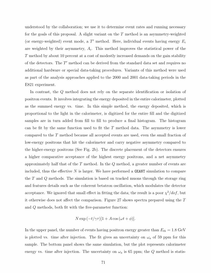
understood by the collaboration; we use it to determine event rates and running necessary
for the goals of this proposal. A slight variant on the T method is an asymmetry-weighted
(or energy-weighted) event mode, a T ′ method. Here, individual events having energy Ei
are weighted by their asymmetry, Ai. This method improves the statistical power of the
T method by about 10 percent at a cost of modestly increased demands on the gain stability
of the detectors. The T ′ method can be derived from the standard data set and requires no
additional hardware or special data-taking procedures. Variants of this method were used
as part of the analysis approaches applied to the 2000 and 2001 data-taking periods in the
E821 experiment.
In contrast, the Q method does not rely on the separate identification or isolation of
positron events. It involves integrating the energy deposited in the entire calorimeter, plotted
as the summed energy vs. time. In this simple method, the energy deposited, which is
proportional to the light in the calorimeter, is digitized for the entire fill and the digitized
samples are in turn added from fill to fill to produce a final histogram. The histogram
can be fit by the same function used to fit the T method data. The asymmetry is lower
compared to the T method because all accepted events are used, even the small fraction of
low-energy positrons that hit the calorimeter and carry negative asymmetry compared to
the higher-energy positrons (See Fig. 2b). The discrete placement of the detectors ensures
a higher comparative acceptance of the highest energy positrons, and a net asymmetry
approximately half that of the T method. In the Q method, a greater number of events are
included, thus the effective N is larger. We have performed a GEANT simulation to compare
the T and Q methods. The simulation is based on tracked muons through the storage ring
and features details such as the coherent betatron oscillation, which modulates the detector
acceptance. We ignored that small effect in fitting the data; the result is a poor χ2/dof , but
it otherwise does not affect the comparison. Figure 27 shows spectra prepared using the T
and Q methods, both fit with the five-parameter function:
N exp (−t/γτ)[1 + A cos (ωt + φ)].
In the upper panel, the number of events having positron energy greater than Eth = 1.8 GeV
is plotted vs. time after injection. The fit gives an uncertainty on ωa of 59 ppm for this
sample. The bottom panel shows the same simulation, but the plot represents calorimeter
energy vs. time after injection. The uncertainty on ωa is 65 ppm; the Q method is statis-
71
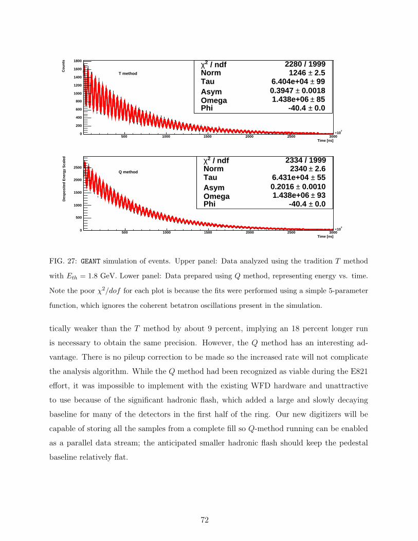
/ ndf 2χ 2280 / 1999Norm 2.5± 1246 Tau 99± 6.404e+04 Asym 0.0018± 0.3947 Omega 85± 1.438e+06 Phi 0.0± -40.4
Time [ns]500 1000 1500 2000 2500 3000
210×
Co
un
ts
0
200
400
600
800
1000
1200
1400
1600
1800 / ndf 2χ 2280 / 1999
Norm 2.5± 1246 Tau 99± 6.404e+04 Asym 0.0018± 0.3947 Omega 85± 1.438e+06 Phi 0.0± -40.4
T method
/ ndf 2χ 2334 / 1999Norm 2.6± 2340 Tau 55± 6.431e+04 Asym 0.0010± 0.2016 Omega 93± 1.438e+06 Phi 0.0± -40.4
Time [ns]500 1000 1500 2000 2500 3000
210×
Des
po
site
d E
ner
gy
Sca
led
0
500
1000
1500
2000
2500
/ ndf 2χ 2334 / 1999Norm 2.6± 2340 Tau 55± 6.431e+04 Asym 0.0010± 0.2016 Omega 93± 1.438e+06 Phi 0.0± -40.4
Q method
FIG. 27: GEANT simulation of events. Upper panel: Data analyzed using the tradition T method
with Eth = 1.8 GeV. Lower panel: Data prepared using Q method, representing energy vs. time.
Note the poor χ2/dof for each plot is because the fits were performed using a simple 5-parameter
function, which ignores the coherent betatron oscillations present in the simulation.
tically weaker than the T method by about 9 percent, implying an 18 percent longer run
is necessary to obtain the same precision. However, the Q method has an interesting ad-
vantage. There is no pileup correction to be made so the increased rate will not complicate
the analysis algorithm. While the Q method had been recognized as viable during the E821
effort, it was impossible to implement with the existing WFD hardware and unattractive
to use because of the significant hadronic flash, which added a large and slowly decaying
baseline for many of the detectors in the first half of the ring. Our new digitizers will be
capable of storing all the samples from a complete fill so Q-method running can be enabled
as a parallel data stream; the anticipated smaller hadronic flash should keep the pedestal
baseline relatively flat.
72
B. Electromagnetic Calorimeters
The electromagnetic calorimeters for the E821 experiment used a Pb/SciFi design [81, 82].
Each calorimeter consisted of a monolithic block of 1-mm diameter fibers arranged in a near
close-packed geometry within grooved lead alloy foils. The fractional composition of the
detector was Pb:Sb:Fiber:Glue = 0.466 : 0.049 : 0.369 : 0.096 (by volume), leading to a
radiation length X0 = 1.14 cm. The fibers were oriented radially so that the positrons
would impact on the detector at large angles with respect to the fiber axis. Four lightguides
directed the light to independent PMTs and the summed analog signal was processed by
waveform digitizers. The 14-cm high by 22.5-cm radial by 15-cm deep calorimeter dimensions
were largely dictated by the available space and the need to have a sufficient radial extension
to intercept the positrons. The energy resolution requirement for (g−2) is relatively modest,
∼ 10% or better at 2 GeV.
For the New (g − 2) Experiment, the systematic errors associated with gain instability
(0.12 ppm) and pileup (0.08 ppm) must each be reduced by a factor of ∼ 3 − 4. We have
designed [15] a new calorimeter that retains the fast response time of plastic scintillating
fiber, but is made from an array of dense submodules where each is oriented roughly tangen-
tial to the muon orbit. This configuration provides transverse segmentation and allows for
multiple simultaneous shower identification. A 50:50 ratio of tungsten to scintillator (and
epoxy) reduces shower transverse and longitudinal dimensions. The calculated [84] radiation
length, X0 = 0.69 cm, is 60% of the length for the Pb/SciFi modules used in E821. Conse-
quently, the modules can be made compact enough to free space for downstream readout in
the highly constricted environment of the storage ring. The high density leads to a smaller
radial shower size, which improves the isolation of simultaneous events. We find that using
0.5-mm layers gives an acceptable resolution close to 10% at 2 GeV for a prototype we have
built and tested; a non-trivial error contribution to this measured performance parameter
came from the beam momentum spread, photo-electron yield and transverse leakage fluc-
tuations in our test environment. Therefore, the intrinsic detector response from sampling
fluctuations alone is better.
A plan view of the vacuum chamber and the detector positioning is shown in Fig. 28,
indicating that this design looks promising for the standard vacuum chamber sections. In
this figure, 20 lightguides are indicated as they curl toward the inside of the storage ring. By
73

FIG. 28: Plan view of new calorimeters and existing scalloped vacuum chamber region.
design, the W/SciFi is a single monolithic array, which can be readout on the downstream
side by any segmentation of optical couplers. The choice of 20 or 35 readouts (4 × 5 array
or 5× 7 array) is an optimization to be determined based on the final readout solution. We
are exploring silicon photomultiplier (SiPM) arrays and will perform tests in the coming
year. At the time of this proposal, several large SiPM arrays are being produced, which
would nicely match the 35-segmented model mentioned above. However, a conservative
solution will be to use PMTs located outside of the field region. It is a solution that we have
considerable experience in implementing based on E821.
Appendix C includes a more detailed description of a tungsten / scintillating fiber (W-
SciFi) sampling calorimeter that meets these demands. In anticipation of this proposal,
we built a 4 × 6 cm2 prototype module made of 0.5-mm pitch layers of fiber ribbons and
pure tungsten plates. Measurements were made at PSI and at FNAL and results have been
reported [15].
C. Position-Sensitive Detectors
In E821, five-fold, vertically segmented scintillator hodoscopes were mounted on the up-
stream side of each calorimeter. To provide impact position information for shower recon-
struction and to obtain a better horizontal and vertical profile, we propose to use a system
of straw detectors in front of each station. These can be relatively simple detector systems
with standard multi-hit TDC digitized readout. The time-start for the straws will be derived
from a summed signal from the calorimeters. The straw system in front of each calorimeter
will provide information for shower impact, pileup identification, and muon loss monitor-
ing. For some stations, a complement of in-vacuum straws will serve as positron traceback
74

detectors, which are needed for beam dynamics imaging. These extended imaging stations
will also provide the data used in the physics analysis for a muon electric dipole moment
(See Section IX).
D. Waveform Digitizers for Calorimeter Readout
The primary data acquisition challenge for a new experiment is the readout and inter-
pretation of the calorimeter signals. For the New (g − 2) Experiment, we intend to gather
this information via waveform digitization, where the PMT analog output waveforms are
continuously digitized at high speed. While waveform digitization was used to great effect in
E821, significant advances in many fields - ranging from high speed analog circuitry to par-
allel computation - will allow us to both dramatically simplify and miniaturize the hardware
while extracting significantly more information from the raw data.
The E821 400 MHz waveform digitizer (WFD) hardware was based on an earlier design
from the MACRO experiment. It consisted of an analog input shaper, a clock input module,
the Flash digitizer itself, a data formatter, discrete RAM banks, and a VME32 interface. The
relatively low RAM densities available at the time coupled with stringent realtime processing
constraints required the time consuming design and high-cost implementation of a custom
data formatting ASIC. Current off-the-shelf and custom WFD designs are generally similar,
but typically contain on-board FIFO memories. The main difference lies in the replacement
of the inflexible custom ASICs with field programmable logic (in the form of FPGAs or
CPLDs). We have deployed such a design for use in the MuLan and MuCap precision muon
lifetime experiments at PSI.
For the New (g− 2) Experiment, we propose a departure from this model. FPGA based
designs excel at manipulating very low level, realtime logic transformations, including such
things as ADC readout, memory controllers, and network transceivers. High level data
manipulation on the devices, however, is complicated by relatively high implementation,
testing, and debugging barriers. These manipulations are much better done in high level
computer programming languages on commodity hardware. We propose a hybrid design
that merges the strengths of each approach, while minimizing engineering, construction,
and deployment costs.
The time structure of PMT pulses requires digitizing the output data stream at 500MHz
75

AnalogShaper
ControlLogic
ClockBuffer
FADC
ClockLogic
FrontendFPGA
BufferRAM
InterfaceFPGA
ROM/Flash
GigEInterface
Logic
WFD Block Diagram
ToDAQ
GigESwitch
Pre-FrontendComputer
FIG. 29: A block diagram of the hybrid waveform digitization system.
with an 8 bit flash digitizer. We will continuously digitize these signals, recording 600 µs of
data per calorimeter segment per fill. Having every sample of each fill permits simultaneous
extraction of T -method, Q-method, and other derived data streams from one digitization
record. Ideally, we would simply send all of this raw data to persistent storage. With 24
calorimeters, however, the total raw data rate is 3-5 GB/s (depending on segmentation),
significantly too great a rate to store completely. The DAQ system needs to reduce this, to
of order 50-100 MB/s; the final value will of course depend on details of the DAQ system
and the available FNAL network infrastructure and data storage resources at the time the
experiment is run. To meet this challenge, the hybrid digitization system will operate in
two stages: a simple hardware digitizer to record the data, and “pre-frontend” computers to
perform all triggering, data selection, and packaging tasks. The hybrid system will present
a configurable set of packaged data streams (e.g. T/Q-method datastreams) to the DAQ
system for collation and storage.
Each WFD hardware channel will consist of analog and clock input stages, a 500 MHz
flash digitizer, buffer memories, the communication interface, and various support modules
(firmware PROMS, programming and test ports, LED feedback, synchronization hardware,
etc.). These will be tied together with one or more FPGAs to move the data at high
76

speed between the various functional blocks (see Figure 29). Minimizing the duration of the
design life cycle is of great importance, and we approach this in part by using off-the-shelf
technologies whenever possible:
• We intend to use standard DDR computer memories in a bank switched configuration,
instead of more expense FIFO memories. This allows simultaneous storage of the
current fill while reading out the previous fill. It also permits use of previously written
and debugged memory controller firmware.
• Every channel will operate independently (although multiple channels may be carried
on one physical circuit board, they should share no processing or interface resources);
this simplifies the firmware for setup and communications, as well as simplifying re-
placement of failed channels.
• The boards will be mounted in VME-style crates to supply the large quantities of power
needed, but the communications interface will be Gigabit (or faster) ethernet. Again,
debugged firmware modules are readily available, and custom interconnect topologies
can be implemented with inexpensive commercial hardware. We may even consider
UDP or TCP transport instead of using raw ethernet communications.
• The raw data can be compressed before transport if necessary. We will utilize a
standard algorithm (such as the LZ77 algorithm embodied in the ubiquitous gzip
library) to minimize implementation and debugging costs.
As each WFD channel is independent, while positrons will typically deposit energy in mul-
tiple calorimeter segments, triggering decisions must be made globally over each calorimeter.
In the past, we might have performed this task in a separate analog module which would
then force digitization in each WFD channel. Recent advances in multicore and parallel
computation (embodied at the consumer level, for instance, in the popular Intel Core2 CPU
architecture) and practical parallel programming techniques will allow us to perform this
task cost effectively with off-the-shelf hardware and software written in a high level lan-
guage. For our needs, General Purpose Graphics Processing Units (GPGPUs), consisting of
multiple high-speed floating point units with hundreds of cores per die, are becoming read-
ily available at low cost. The available programming interfaces, such as NVIDIA’s CUDA,
77

AMD’s Stream, and the developing OpenCL standard hide the complexity of data transfer
and core scheduling, permitting relatively simple access to these massively parallel resources.
Each calorimeter station, then, will have a dedicated “pre-frontend” computer that will
perform WFD readout and triggering for a given calorimeter. This pre-frontend will decom-
press and reformat the WFD data to optimize computation speed. It will then perform a
number of parallel computations over each calorimeter:
• For the T -method, equal-time samples must be summed over all calorimeter segments,
triggers identified, and “data islands” formatted and written to a data stream.
• For the Q-method, blocks of consecutive samples must be decimated and summed
across calorimeter segments. Successive fills can being summed together to further
reduce the data rates.
• A potential new approach to pileup correction sums multiple successive fills before
performing the T -method triggering decisions. This additional “Pileup T -method”
stream could be easily derived from multiple recorded streams, and saved along with
the standard T -method data set.
• Occasionally, entire fill records should be stored for detailed studies of, for instance,
gain and pedestal stability.
Each of these potential computations, and others that are identified in the future, can be
independently formatted, packaged and presented to the DAQ system for persistent storage.
By performing all of this high level physics in software we can defer the actual specification
of the final data streams until very late in the experiment, once physics studies and data
acquisition performance tests have been performed.
E. Clock systems
A time base having 0.01 ppm absolute accuracy and stability over several months is not
difficult to obtain; vendors such as Precision Test Systems and Agilent provide inexpensive
synthesizers driven by ovenized oscillators which meet that specification. In the MuLan
experiment, for instance, the 500MHz system clock which drove the WFDs was generated
with an Agilent E4400 synthesizer. Extensive comparisons with external standard oscillators,
78

both before, during, and after the experiment, confirmed the stability and accuracy claims
of the manufacturer. The long term stability of such devices can be economically extended
to cover the multiyear duration of this experiment by slaving the master synthesizers to a
common GPS-disciplined 10MHz frequency standard.
Similar synthesizers will be used in the present experiment to drive the various acquisition
and NMR systems. We have extensive experience in distributing similar clock signals in other
precision experiments, using low skew linear fanout and amplifier modules from companies
such as Miniciruits. The final component of the clock system design is a robust blinding
methodology; we hide the absolute clock frequencies from the ωa and ωp analysis teams until
the analysis is completed. These are well understood techniques with very low design and
implementation risks.
F. Data Acquisition
By comparison to E821 the New (g − 2) Experiment will record about 21× the de-
cay electrons at ∼1.5× the rate per fill and ∼6× the rate per second. Moreover, the ex-
periment will record the signals from the individual calorimeter segments rather than the
calorimeter-segment sums, and record T -method datasets (comprising digitized pulses is-
lands), Q-method datasets (comprising digitized fill periods) and other derived datasets. In
addition, the new readout must incorporate the new straw counter arrays and account for
the different beam time structure.
The new data acquisition must handle both very high data rates (∼80 MB/sec) and very
large raw data volumes (∼1 PB total). It must transfer both the event data from various
detector sub-systems to the mass storage devices and the experimental parameters from the
various diagnostic sub-systems to an experiment database. Moreover, the readout system
must be deadtime-free during the measuring periods in order to avoid any distortions of the
time spectrum of the decay positrons. Finally, the DAQ must be flexible enough to use for
the installation, testing, diagnostic and production phases of the experiment.
The DAQ (see Fig. 30) will be implemented as a modular, distributed acquisition system
on a parallel, layered processor array using multi-threaded PC’s, a Linux platform and a
multi-layered Gbit network. A frontend (FE) layer will be responsible for the readout of
the calorimeter segment waveforms, straw counter hits and other detector sub-systems. The
79

FIG. 30: Schematic layout of the anticipated DAQ system.
backend (BE) layer will be responsible for both the assembly of data fragments into complete
events and the permanent storage of the complete events. A slow control layer will be
responsible for the control and monitoring of diagnostic instrumentation associated with the
ring, detectors and other sub-systems. Finally, an online analysis layer will be responsible for
the integrity-checking and basic histogramming that ensures the overall quality of recorded
data.
The primary source of high-rate data is the twenty-four calorimeters. As described earlier,
each calorimeter segment is instrumented with one waveform digitizer channel that transmits
packets of 500 MHz, 8-bit, continuous digitization (CD) data to so-called pre-FE processors.
These pre-FE processors derive the Q/T -method data-streams and transmit the resulting
derived databanks over the FE network to the FE layer of the data acquisition. We expect
a total rate of calorimeter Q/T -method data of roughly 80 MB/sec.
80
A second source of high-rate data are the straw counter arrays. We envisage a straw
counter readout system based on commercial VME multi-hit TDCs and VME-to-PCI inter-
faces that deliver their data to a dedicated FE processor on the FE network. We expect a
total rate of straw counter data of several MB/sec.
The backend layer will receive data fragments from the various frontend processors across
the frontend network, assemble the event fragments into complete events, and copy the events
to mass storage. Each event will represent a time-ordered history of the calorimeter, straw
counter, and other detector data for one entire fill. For mass storage we propose to store one
copy of the data on the Fermilab tape archive (i.e. the Fermilab Enstore system or its future
equivalent) and one copy of the data on a large disk array (e.g. a BlueArc storage node or
its future equivalent). The event building will utilize backend local memory segments for
temporary buffering of event fragments and the data logging will utilize backend local disks
for temporary buffering of complete events.
The slow control layer is essential for careful monitoring of systematic issues and will
incorporate the readout of instrumentation such as HV controls, current monitors, temper-
ature sensors, field probes and scalars. The slow control readout will operate in periodic
mode and be asynchronous to the beam cycles, DAQ cycles, etc. The slow control data will
be written to both the mass storage devices and the experimental database.
The online analysis layer will provide the integrity checks and diagnostics plots that ensure
the quality of recorded data. The online analysis system will be resident on a dedicated
network and receive events as ‘available’ from the backend layer (in order to avoid the
introduction of unnecessary deadtime). The system will provide for both local and remote
access to the experimental data.
VIII. SYSTEMATIC UNCERTAINTIES ON ωA
In this section we consider the primary systematic errors on the ωa analysis, which totaled
0.19 ppm in the final run of E821. [104] Our goal in the New (g− 2) Experiment is a factor
of 3 reduction for a total of ≤ 0.07 ppm. This goal can be met by incorporating a suite
of improvements to the experiment. Here, we briefly outline the plan to reduce the largest
sources of systematic error: gain changes, lost muons, pileup, coherent betatron oscillations,
and the uncertainty associated with the electric field and pitch corrections. Table IX lists the
81

final E821 uncertainties and projections for improvements in the New (g − 2) Experiment.
The traditional T method analysis is assumed because uncertainties can be reliably projected
based on our considerable experience in these analysis efforts. Since the Q method is new,
we have not included its positive and partially independent impact on the final statistical
result, nor are we able to fully project associated systematics. One key attractive feature
of the Q method is pileup immunity; there is no correction necessary so that systematic
uncertainty is absent. Comparing the analysis results using both T and Q methods will
provide a valuable confirmation that systematic errors are understood.
A. Gain Changes and Energy-Scale Stability
The hardware gains of the detectors were determined to be stable to ≈0.15% from early
to late times within a storage ring fill. This limit was established by plotting the average
energy for each (g − 2) period versus time after the PMTs were switched on. The gating
circuitry in the base that allowed the PMTs to be turned off to avoid the initial burst of
pions entering the ring, also resulted in a variation in the gain. For gain variations like this
one, where the time constant is long compared to the (g−2) oscillation period, the coupling
to the ωa frequency is small and after correction the residual systematic error is less than
0.02 ppm.
If the gain oscillates at a frequency ωa, with an amplitude that varies in time, and with a
phase that differs from that of the ωa oscillation of the positron sample, then a direct error
on the measured value of ωa is produced. The average rate at which energy is deposited
into the calorimeters oscillates with frequency ωa, and therefore any rate dependence in
the gain of the detectors produces gain oscillations. We were able to demonstrate that
the gain dependence on rate was small enough that its effect on ωa was typically less than
0.03 ppm. In the new experiment, the slightly increased beam rates will be offset by increased
detector segmentation. In E821, a UV-laser system was used to periodically pulse the
scintillator in the detectors and thus monitor the complete gain and reconstruction chain
during data collection against an out-of-beam reference counter. Unfortunately, the light
distribution system included too many branches and only one upstream reference detector.
Small fluctuations cascaded so that gain stability could be monitored to no better than a
few tenths of a percent. At PSI, we have recently built and used a simplified version of
82
this system, which monitors hardware gains at the sub-0.1% level by having a monitor on
a parallel level to that seen by the detectors. We intend to incorporate a similar system in
the New (g − 2) Experiment to largely eliminate this uncertainty.
The greater contribution to the gain systematic error came from artificial gain oscillations
at the ωa frequency, introduced by the data reconstruction software. Here, the “energy-
scale” stability is related to software reconstruction of waveforms. When a signal was above
the WFD hardware threshold, a pre-set minimum number of sequential WFD samples was
recorded. These data were fit offline for the peak plus linear background to deduce the
energy and time of the positron. But, if the trigger pulse was followed or preceded closely
by another pulse, both pulses were fit together with a common background term, and the
fitting region becomes longer compared to that used for a single pulse. The fitted energy
was found to depend slightly on the length of the fitting region and the fitting samples were
fixed in number by hardware. Because the data rate oscillates at frequency ωa, and is higher
at early than at late decay times, it follows that the fitting region length oscillates at ωa
and is, on average, longer at early times compared to late times. This produces a small,
effective gain oscillation with frequency ωa whose amplitude decreases with time, leading
to a systematic error on ωa. Given the current capabilities in data throughput, the new
electronics will record all samples in place of isolated islands, thus removing the source
of this reconstruction bias. In summary, the larger of the gain systematic pieces will be
eliminated by design and the smaller contribution will be monitored more precisely.
B. Lost Muons
“Lost muons” refers to muons that escape the storage ring before they decay. These losses
were about 1% per lifetime at early decay times and decrease to about 0.1% at later decay
times in the BNL experiment. One consequence of losses is that, in a fit to the data, the
lifetime is not quite correct. This is a slow change in the spectrum, having no ωa frequency
component; therefore the correlation to ωa in the fit is small. However, even though the
correlation is small, neglecting muon losses in the fit in E821 would have shifted the ωa
frequency by 0.18 ppm and resulted in a very poor χ2 from the fit. By monitoring the muon
losses with hodoscopes on the front of 14 of the calorimeters in E821, the muon loss profile
was constructed and the resulting uncertainty was held to better than 0.03 ppm. In the
83

upgraded experiment, all 24 calorimeters will incorporate muon sensitive detectors, straws
or scintillator, allowing muon losses to be monitored around the entire ring. Furthermore, an
open-ended inflector will reducing scattering as the muons enter the storage ring, resulting
in smaller losses. Finally, muon losses can be greatly reduced when an effective “scraping”
strategy is employed. During scraping, the stored muon orbit is shifted so that outliers in
the phase space are lost on collimators during the first 20 µs after injection. In the 2nd
half of the final E821 run, this technique resulted in an order of magnitude reduction in the
losses during the ωa fitting period.
The muon losses entry in Table IX arises mainly from the uncertainty in the possible
difference between the average phases for stored and lost muons. For example, one source
of muons, carrying a different phase and potentially lost at a higher rate, are those created
after the momentum-selecting slit just upstream of the inflector. These muons, born from
pion decay in that short region, have a different phase compared to those captured in the
decay channel (the later muons did not go through the final dipole bend, which precesses
the muon spin). In a 900-m long decay channel as we assume at FNAL, the population of
muons born in the last turn into the storage ring will be essentially negligible and will be
dwarfed fractionally by those born in the long AP2 decay channel. While this uncertainty
can almost be eliminated, we include a small estimate here of 0.02 ppm for smaller possible
contributions to the fitting.
C. Pileup
The error due to pileup scales linearly with rate in each segment of the detectors. The
effective size of the segment depends on the geometric extent of the shower. A simulation
was used to demonstrate that the new W/SciFi calorimeters, having 20 or 35 independent
segments, and a smaller Moliere radius, will provide an effective five-fold reduction in the
intrinsic pileup. With no further improvements, and the proposed factor of up to 3 increase
in data rate, the pileup error would be reduced by at least 3/5 to 0.048 ppm. While we
could accept this level of error, some improvement is desirable and achievable.
In the past, an artificial pileup spectrum was constructed from individual pulses in the
data, then subtracted from the raw spectrum. In the pileup construction, it is necessary to
use pulses with pulse heights below as well as above the hardware threshold. Because of
84
the relatively high hardware threshold and limited storage of the E821 WFD system, those
pulses below threshold were only found by searching during the relatively short period of
continuous WFD digitization following the trigger generated by the presence of a large pulse
above threshold. Consequently, the sample size for pileup events was limited and somewhat
biased, since they had to always ride on the tails of larger pulses. In the new data WFD and
data acquisition scheme, it will be possible to significantly improve the pileup construction
process. Continuous digitization, with local software sorting of data streams including T -
method, Pileup T -method and Q-method datasets, is anticipated. Pulses of all heights can
be searched for independent of whether there is a nearby large pulse that fired a hardware
trigger.
In E821, signals from four detector segments were combined before WFD digitization.
Any mismatch in the relative timing of these signals can lead to variation in the pulse shape
of the sum. In addition, the scintillator fiber in the calorimeters was strung radially, causing
the pulse shape to depend slightly on the radial entrance position into the detector. These
variations in the pulse shape hampered efforts to handle pileup, both in the fitting of two
nearby peaks, and in the process of constructing the pileup spectrum. The pulse shape is
expected to be more stable in the new design, because each segment will be individually
digitized. In addition, the E821 WFDs were composed of two 200 MHz ADCs that sampled
the pulse shape out of phase and were later stitched together to form a 400 MHz record. The
upgraded experiment will employ single phase 500 MHz WFDs based on a similar design
that we have already successfully used in muon lifetime experiments at PSI.
The contribution of pileup to the error in ωa for E821 was divided into three components.
The first two are correlated and add linearly. The third is not correlated so it is added in
quadrature to the other two.
1. Pileup efficiency, 0.036 ppm. This is due to an estimated 8% uncertainty in the
amplitude of the constructed pileup spectrum.
2. Pileup phase, 0.038 ppm. This is the error due to the uncertainty in the phase of the
constructed pileup spectrum.
3. Unseen pileup, 0.026 ppm. This is the error due to pulses so small that they cannot
be reconstructed and therefore they are not included in the pileup construction.
85

We expect that the lower rate per detector segment in the new experiment, coupled with
the new full-energy data stream will lead to a comprehensive pileup correction with minimal
uncertainty. We assign up to 0.04 ppm here to account for any difficulties in the anticipated
analysis. As mentioned earlier, the Q method is complementary to the traditional T method
and has different sources of systematic errors. The most significant difference is the effect
of pileup—it is greatly reduced for the Q method.
D. Coherent Betatron Oscillations
The average position and width of the stored beam can vary as a function of time as
the beam alternately focuses and defocuses in the ring. This imposes an additional time
structure on the decay time spectrum because the acceptance of the detectors depends on
the position and width of the stored muon ensemble.
The CBO frequency lies close to the second harmonic of ωa, so the difference frequency
ωCBO−ωa can be quite close to ωa, causing interference with the data fitting procedure and
thereby causing a significant systematic error. This was recognized in analyzing the E821
data set from 2000. In the 2001 running period the electrostatic focusing field index was
adjusted to minimize this problem. This greatly reduced the CBO systematic uncertainty.
We will follow this tuning strategy again.
In addition, several efforts are underway to reduce the CBO effect even further. They
include:
1. Improve the kicker pulse shape to better center the beam on orbit.
2. Use active RF schemes at very early decay times to reduce the amplitude of the CBO
(see Appendix B).
3. Use an octupole E or B field at very early decay times to damp out the CBO amplitude
(see Appendix B).
4. Increase the vertical size of the detectors. This reduces losses of positrons passing
above or below the detector, reducing sensitivity of the detector acceptance to beam
position and width.
The combined efforts should reduce the CBO uncertainty by a factor of 2 to 0.04 ppm.
86
E. Electric Field and Pitch Correction
With a vertical magnetic field By and radial electric field Er, the precession frequency is
given by
ωa = − q
m
[aµB −
(aµ − 1
(γ2 − 1)
)βEr
]. (34)
If By and Er vary with position, the time averages 〈By〉 and 〈Er〉 should be used. At exactly
the magic momentum the effect from Er is zero. Muons of slightly higher momentum δp
have an equilibrium orbit
xe =Ro
1− n· δp
p.
As they oscillate about this equilibrium orbit they experience a mean electric field 〈Er〉 =
n (βBy/R0) xe and their deviation from the magic momentum is proportional to xe. This
leads to a correction to ωa proportional to x2e. In this experiment n is measured from the
observed horizontal betatron frequency, and the distribution of muons with respect to xe is
found from the modulation of counting rate by the rotation frequency of the muon bunch.
The observed value of < x2e > was confirmed by simulation. The correction is 0.46 ppm.
With electric focusing, the plane in which the muon spin is precessing oscillates vertically,
exactly following the oscillation of the muon momentum. When the orbit is inclined at angle
ψ to the horizontal, ωa is reduced by the factor (1 − 12ψ2). If ψm is the angular amplitude
of the vertical oscillation, the average over the ensemble of muons is (1− 14〈ψ2
m〉) where the
brackets indicate an average over the muon population, 〈ψ2m〉 = n〈y2
m〉/r2o where ym is the
amplitude of the vertical oscillation.
Information on 〈ψ2〉 is obtained by simulation in which a representative set of muons is
tracked around the ring from the inflector exit, via the kicker magnet, for many turns. The
discrete quadrupole structure and aperture defining collimators are included as well as the
calculated deviations from a pure quadrupole field. The pitch correction is +0.29 ppm.
A combined (correlated) electric field and pitch correction uncertainty of 0.05 ppm was
used in E821. We expect to improve on our knowledge of the electric field and pitch correc-
tions by use of a new muon traceback system that can better image the beam motion versus
time at a number of azimuthal positions around the ring. Furthermore, our simulation effort
has improved, which is essential to some of these corrections. It is certainly feasible to reduce
the uncertainty on these important corrections and we estimate a final combined error of
0.03 ppm.
87

TABLE IX: The largest systematic uncertainties for the final E821 ωa analysis and proposed
upgrade actions and projected future uncertainties for data analyzed using the T method.
E821 Error Size Plan for the New (g − 2) Experiment Goal
[ppm] [ppm]
Gain changes 0.12 Better laser calibration and low-energy threshold 0.02
Lost muons 0.09 Long beamline eliminates non-standard muons 0.02
Pileup 0.08 Low-energy samples recorded; calorimeter segmentation 0.04
CBO 0.07 New scraping scheme; damping scheme implemented 0.04
E and pitch 0.05 Improved measurement with traceback 0.03
Total 0.18 Quadrature sum 0.07
F. ωa Systematic Uncertainty Summary
Our plan of data taking and hardware changes address the largest systematic uncertain-
ties and aims to keep the total combined uncertainty below 0.07 ppm. Experience shows
that many of the “known” systematic uncertainties can be addressed in advance and mini-
mized, while other more subtle uncertainties appear only when the data is being analyzed.
Because we have devised a method to take more complete and complementary data sets,
we anticipate the availability of more tools to diagnose such mysteries should they arise.
Table IX summarizes this section.
IX. PARASITIC MEASUREMENT OF THE MUON ELECTRIC DIPOLE MO-
MENT
As has been discussed earlier, the magnetic moment of the muon is a sensitive probe for
new, TeV scale, interactions. If the new interactions also contain CP violating phases, these
phases will give rise to an electric dipole moment (EDM) of the muon. Contrary to the muon
magnetic moment, there is no EDM expected in the Standard Model at a measurable level
and thus any signal indicates new sources of CP violation beyond the Standard Model [85].
As noted in several places, the search for extra sources of CP violation is strongly motivated
since the CP violation observed in the quark sector so far is insufficient to explain the matter
dominance of the universe [86].
88

If the CP violating phases of the new interactions are independent of lepton flavor, the
muon EDM will be related to the electron EDM by simple mass scaling. In this case,
the current electron EDM limits rule out the ability to discover a muon EDM with the
g-2 experiment proposed here. However, as discussed below, a muon EDM measurement
performed with the proposed experiment could potentially extend the exclusion of flavor
dependent CP violating interactions by 2 orders of magnitude.
The phenomenology of a muon EDM is described in detail in Ref. [87]. The muon dipole
moment is related to the muon spin by
~dµ =q
2mηµ~s
with ηµ playing a similar role to the g factor for the magnetic moment. The muon precession
receives components from both anomalous magnetic moment, aµ, and ηµ. At the magic
momentum we have
~ωa = − q
maµ
~B,
~ωEDM = − q
2mηµ
~β × ~B +
~E
c
= − ηµ
2mc~F .
From this one sees that a muon aligned with the magnetic field will experience a torque that
will act to tilt the precession plane away from the vertical direction by an angle
δ = tan−1(ηµβ/2aµ).
One also sees from the above equation that the modulation in the vertical plane is sinusoidal
and thus 90 out of phase with the aµ modulation.
The E821 collaboration has recently submitted for publication a measurement of the
muon EDM by including an up-down asymmetry, offset by 90 in the ωa fit yielding an
upper limit of |dµ| < 1.8 × 10⁻¹⁹ e cm [87] which is a factor of 5 improvement over the
previous best limit [88]. Results of the fit are displayed in Fig. 31. The measurement was
performed in part using straw tube tracking detectors [89] that were designed to determine
the muon beam distribution within the storage ring and instrumented in front of one of the
24 calorimeter stations.
89

FIG. 31: Data recorded by the E821 traceback system. The left distribution is the number of
tracks versus time modulo the precession frequency. The right distribution is the average vertical
angle of the tracks versus time also modulo the precession frequency.
A. E821 Traceback System
A replication of the E821 traceback system is required for the proposed g-2 measure-
ment. The available statistics for a muon EDM measurement could be greatly increased
by instrumenting several more calorimeter stations with tracking capability. This can be
accomplished by placing the straw tracking chambers inside the vacuum chambers in the
scallop region in front of the calorimeters.
A similar number of channels to the E821 traceback system can be mounted on extra
vacuum ports that exist and are not instrumented in most scallop regions as indicated in
Fig. 33. A final layer can be placed outside the vacuum, directly in front of the calorimeters.
While 23 additional calorimeter stations exist, several of them do not have a clear line
of sight to the muon beam due to quadrapole magnets or other instrumentation so that
instrumenting all stations with tracking capabilities may not be feasible.
Besides increasing the statistics for an EDM measurement, increased tracking instrumen-
tation will allow the beam profile to be measured at several locations around the ring. This
will be very useful input to beam simulation and it is expected to lead to a reduction in the
errors associated with the electric field pitch corrections from 0.05 ppm to 0.03 ppm.
90

Muon Orbit
Decay positrontrajectory
Muon decay point
~2 m
VacuumChamberWindow
Calo20Calo19
TB1 TB2 TB3 TB4
FIG. 32: Top view of the E821 traceback straw tracking system.
B. Improved Traceback System
A replication of the E821 traceback system is required for the proposed (g−2) measure-
ment. The available statistics for a muon EDM measurement could be greatly increased by
instrumenting more calorimeter stations with tracking capability. This can be accomplished
by placing the straw tracking chambers inside the vacuum chambers in the scallop region
in front of the calorimeters. In this position, the acceptance of the chambers is greatly
increased compared to that of E821.
A similar number of channels to the E821 traceback system can be mounted on extra
vacuum ports that exist and are not instrumented in most scallop regions as indicated in
Fig. 33. A final layer can be placed outside the vacuum, directly in front of the calorimeters.
While 23 additional calorimeter stations exist, several of them do not have a clear line
of sight to the muon beam due to quadrupole magnets or other instrumentation so that
instrumenting all stations with tracking capabilities may not be feasible.
An R&D program is underway at Fermilab to demonstrate the feasibility of such a track-
ing system. This program builds largely on experience gained from the CKM R&D program
to develop straws in vacuum [90] and current efforts to develop straws for improved instru-
mentation of the meson test beam area (MTest). Fermilab is also developing a Geant4 based
simulation to determine the overall requirements of the system such as the allowed material
budget, the effects of pileup and other beam backgrounds, and the effects of material, such
as the quadrupoles, that exist between the muon beam and the location of the tracking
stations.
91

Availableports
FIG. 33: Top: Beam Pipe schematic indicating available vacuum ports where straw tracking
chambers can be placed. Bottom: picture of available ports.
92

X. MANPOWER, COST ESTIMATE AND SCHEDULE
A. Manpower
We have formed a new collaboration to carry out this measurement, which represents a
healthy ratio of former E821 collaborators along with strong new institutions. Fortunately,
much of the expertise built up in E821 is represented and still available to us. We still
have senior experts in the collaboration who cover all of the different technical areas. New
institutions bring creative input and additional technical capabilities. These groups include
the host laboratory—Fermilab—and new university groups at James Madison, Kentucky,
Massachusetts, Michigan, Regis, and Virginia. New international groups include KEK and
Osaka from Japan, KVI-Groningen from The Netherlands, Frascati from Italy, and PNPI
from Russia. The Muons Inc. team has also joined the effort. In some cases, experienced
younger E821 collaborators are associated with their new institutions. The names listed
on the proposal masthead are mainly senior physicists. As the experiment develops, we
expect postdocs and students to sign on; indeed, with approval, we will immediately begin
a vigorous campaign to enlist the talents of young people. We are proud that E821 offered a
rewarding experience for dozens of postdocs and graduate students and we intend to welcome
young physicists in the new effort.
B. Cost Estimate
The New (g− 2) Experiment is based on the well understood efforts associated with the
BNL E821 experiment. We intend to utilize a large fraction of available custom instrumen-
tation from that effort, principally the storage ring magnet and its internal and supportive
subsystems. New to the FNAL experiment will be the beam delivery scheme and improve-
ments in the precession and field measurement instrumentation that will permit reduction
of systematic errors.
The tasks and costs fall into three main areas.
1. Beamline
The transformation of the existing FNAL rings and accelerator complex toward hosting
experiments at the intensity frontier involves upgrades to the Booster, transfer lines
93

into and out of the Recycler, RF upgrades to the Recycler, modifications of the AP0
pulsed dipole magnet, additional quadrupoles in the AP2 transfer line, an extraction
port from the Debuncher, the opening of certain fixed apertures in the AP3 transfer
line, and finally a new short beamline stub into the muon storage ring. Many of the
items are required for the approved Mu2e experiment and would be required for any
other high-intensity experiment based on the 8-GeV proton beams. We identify those
items that are unique to the New (g− 2) Experiment in our Table of costs. The costs
for some entries have only been estimated at this time. We note that none are risky
developments and none require any high-degree of technical design.
2. The Storage Ring
The superconducting storage ring, its power supplies, internal subsystems such as the
vacuum system, electrostatic quadrupoles, kicker, pickup electrodes, fiber monitors,
and the external FODO beamline and beamline stub into the ring all exist. They are
available to us from BNL under laboratory and DOE agreements (which will have to
be formalized). These items must be packaged and transported from BNL to FNAL
and reassembled. BNL engineers have estimated the costs for the ring disassembling,
shipping, and reassembly at FNAL. FNAL experts estimated the costs for a new
temperature-stable building and for necessary cryo and power connections. Because
the transport of such an instrument carries risk, we included a 100% contingency for
this effort. The re-assembly—mostly labor—is assigned at 50% contingency.
3. Detector and Measuring Systems
The magnetic field measuring system will be upgraded. It is of relatively modest cost
and will be provided for by the collaboration. A new set of electromagnetic calorime-
ters, their optical readout and waveform digitizers, are also required. Prototypes have
been built and bids for production quantities have been made for the detector. Wave-
form digitizers have been designed and built by our collaboration and costs for a new
system are relatively well understood. The data acquisition system will be new. Straw
detectors and their readout are required for each calorimeter station. We estimate that
most of the costs for the detector and measuring systems will come from collaborating
institutes with support from their respective funding agencies through supplemental
support. We also plan for support in this area from our international collaborators.
94
Figure 34 shows tables that summarize the cost estimates as we now know them. Below
the figure is a set of notes referring to the individual entries. Many of the local FNAL
estimates have been made by experts, but they are not based on detailed studies. Estimated
contingencies and overhead appropriate to the entry and risk are included. Notes provided
below the table indicate sources and other information where available. If Stage 1 approval is
awarded, will we begin a thorough design and cost review for the beamline and ring relocation
associated costs, which drive the budget. It is our intention to keep the total project costs
as lean as possible, while still providing a high-impact, state-of-the-art precision experiment
that can be built and run in the near-term.
We divide the cost tables into two general categories. In the shaded yellow box are items
required for a FNAL based high-intensity proton program (many of these are in progress
now). We believe these items will have longer term benefits, from more smoothly leading
up to Mu2e operation, to opening the possibility of other experiments not yet proposed,
which will require custom beam structures and high intensity. Specific to the New (g − 2)
Experiment are items shaded in green. The (g − 2) Table includes a column specific to
DOE-HEP (mainly beamline and ring relocation) and one that we expect to obtain from
support to NSF user groups and from our international partners. The numbers in the tables
include contingency.
95

FIG. 34: Preliminary Cost Estimate for the New (g − 2) Experiment. Rates used for labor
estimates were $228k/FTE for engineering, $130k/FTE for technician effort, and $135k/FTE for
drafting/design. The yellow table is generic for a high-intensity proton program at FNAL (including
the Mu2e Experiment.) The green table is specific to the New (g − 2) Experiment. Costs in the
table include contingencies.
1. FNAL AD/RF technical note
2. Part of the NOvA project; required for (g − 2)
3. FNAL AD/RF technical note
4. FNAL AD/EE technical note
5. Estimate based on NOvA project, Boo2RR line
6. Kicker magnet & PS; FNAL AD/EE
96
7. Estimate for new magnet
8. Estimate to bring quads from BNL, install; stands, etc.
9. Estimate to move transfer line to AP3 from ACC to DEB ring
10. Estimate; not designed
11. Estimate; not designed
12. Shipping based on commercial quotes and BNL engineer estimates of labor; includes
100% contingency
13. Assembly based on BNL manpower and time estimates; includes 50% contingency
14. FNAL AD/Cryo presentation 9/08
15. FNAL FESS; 25%contingency; includes EDIA and indirect
16. Commercial Quotes plus experience building similar systems
17. Tolkin Quote in Japan
18. Collaboration estimate
C. Schedule
Assuming approval of this proposal, we outline the technically driven schedule. If we
obtain CD–0 in mid-2009, then work can begin over the next 12 months—in parallel—on
three main fronts:
1. Detailed beamline calculations and design of the stub into the storage ring. Final
building plans and final citing decisions.
2. Inventory of all BNL equipment that will be available for the New (g−2) Experiment.
Detailed procedure for decommissioning the storage ring and a complete shipping plan.
3. R&D for the calorimeter readout using SiPMs, tests with a new full-scale prototype,
and R&D for in-vacuum straw detectors. A design and prototype for the out of vacuum
straw chambers.
97
With construction funding available, it will take approximately 1 year to build the new ring
housing at FNAL, 1 year to install and make operative the storage ring, and 1 year (with
cryo and power) to shim the magnet to high field uniformity. This sequence drives the
schedule and permits experiment commissioning in the mid-2013 (or, three years following
funding). In parallel, the beamline modifications will be made and the detector systems will
be built and tested. As part of our plan, selected beamline rate tests can be made earlier
with modest impact on the main program.
XI. PLANNED R&D EFFORTS
While the New (g− 2) Experiment is designed largely following the successful existence
proof from BNL E821, it is a challenge to increase the statistics by more than a factor of 20
and reduce the net systematics uncertainties by a fact of 3. Here, we outline some of the
main anticipated R&D efforts, where an expedient effort can influence the final design and
cost reliability. Many other R&D efforts are presented in previous sections.
• Lithium Lens Pulsing at 18 Hz. The existing antiproton target and lithium
lens system are envisioned for use by our experiment. The fundamental difference
between the current operation with antiprotons and the demands for (g − 2) are
higher repetition rate (0.5 Hz → 18 Hz), but at lower proton energy (120 → 8 GeV).
The lithium lens pulsing system must be studied and possibly tested to determine if
it can operate under these conditions.
• Decay Channel Optimization. Table VI lists several upgrades to significantly
improve the muon storage efficiency per proton. Several others are under consideration.
Detailed studies are required to make the most complete and cost-effective choices.
These studies include: optimization of the beam focus on the target; optimization of
the Li lens optics; complete an end-to-end decay simulation model of AP2 beam line
including additional quadrupole elements; optimization of the optics for maximum
magic muon collection; and, simulate the full transport chain through the inflector
and study transmission into ring with closed/open inflector versions and beam kicker
variants.
98
• Beamline test program. FNAL offers the attractive option that key factors con-
tributing to the anticipated stored muon rate can be verified in beam tests in the near
future. While the final experiment needs the dedicated pulse structure, the foreseen
intensity tests can be performed with booster batches brought on target through the
current main injector beamlines. A test program including required instrumentation
will be designed.
• Half-Length Kicker Plate Test. A prototype kicker plate system exists in a straight
vacuum chamber at BNL. To reduce the inductance of the kicker LCR pulse-forming
network, we can build a half-length kicker system and test it with existing equipment.
The outcome could provide a relatively straight-forward method of improving the
fast muon kicker waveform, and thereby increasing the muon storage efficiency. This
modification would require the construction of three additional kicker modulators to
drive the shorter kicker sections, and a re-working of the modulator housings.
• Tracking of the Magnetic Field. The measurement of the average magnetic field
in experiment E821 relied on continual measurements with fixed probes above and
below the muon storage region. These probes measured the field with respect to mea-
surements with the field trolley, which was calibrated with a plunging probe and an
absolute field probe. In E821 about half of the fixed probes could not be used effec-
tively, due to their proximity to the joints in the precision pole pieces and yoke and the
resulting field inhomogeneity. A detailed R&D effort to re-optimize the fixed probe
configuration around the storage ring would increase the number and effectiveness of
the fixed probes, and should thereby be expected to improve the tracking uncertainty
in the dipole field between field measurements with the trolley. The tracking of higher
multipoles should benefit greatly from the placement of probes besides the muon stor-
age region. These probes would need to be placed in vacuum near the horizontal
quadrupole plates, and a system that can operate in this environment would need to
be developed.
• Large-Scale W/SciFi Prototype and SiPM Readout. We intend to build a near
full-scale calorimeter prototype, which can be readout by both conventional PMTs and
new SiPM arrays. The comparison for pileup, gain stability, easy of assembly, and the
99
final segmentation will be part of the investigation. As with past prototypes, we would
use the FNAL Meson Test area for beam related tests.
• In-vacuum Straw Chambers. To make higher precision images of the beam dy-
namics, monitor muon losses, and to enable a high-statistics measurement of the muon
electric dipole moment, we plan to deploy a set of wire chambers on the face of each
calorimeter with a paired set placed directly upstream in vacuum. A test setup is
underway now at FNAL to investigate this concept and work out the technical details
of placing the straws in vacuum.
XII. SUMMARY OF THE REQUEST
We propose to improve the current measurement of the muon anomalous magnetic mo-
ment aµ by a factor of 4. Combined with expected progress on the theoretical value, a
0.14 ppm result will nearly triple the sensitivity of the measurement to standard model
extensions. The present suggestion from the final E821 result of a standard model violation
may be contradicted, or verified, but whether the new result agrees with the standard model
or not, it will place important constraints on candidate models of new physics—especially
in the context of eagerly anticipated data from the LHC.
In this proposal, we have identified a timely and cost-effective method of using the FNAL
beam complex in the post-Tevatron era to produce custom, high-intensity bunches of muons
that can be injected into the existing superconducting storage ring. While a major task
will be the relocation of the ring from Brookhaven to FNAL, it is work carrying relatively
low risk. The proposed experiment builds on the considerable expertise developed over
more than 20 years in the design, construction, data taking and analysis efforts from E821.
The collaboration has been re-invigorated with many strong new groups who will work in
concert with experts from the previous measurement. The physics motivation is compelling
and promises to continue to provide unique insight into fundamental questions in high-energy
physics.
100

[1] J. Schwinger, Phys. Rev. 73, 416 (1948).
[2] G.W. Bennett, et al., (Muon (g − 2) Collaboration), Phys. Rev. D 73, 072003 (2006).
[3] Eduardo de Rafael Present Status of the Muon Anomalous Magnetic Moment; To appear in
the proceedings of 14th High-Energy Physics International Conference in Quantum Chromo-
dynamics (QCD 08), Montpellier, France, 7-12 Jul 2008. e-Print: arXiv:0809.3085.
[4] G. Charpak, F.J.M. Farley, R.L. Garwin, T. Muller, J.C. Sens, and A. Zichichi, Phys. Lett.
1, 16 (1962).
[5] J. Bailey et al., Nuovo Cimento A9, 369 (1972).
[6] J. Aldins, S.J. Brodsky, A.J. Dufner and T. Kinoshita, Phys. Rev. D 1, 2378 (1970).
[7] J. Bailey et al., Nucl. Phys. B150, 1 (1979).
[8] The g − 2 Collaboration: R.M. Carey et al., Phys. Rev. Lett. 82, 1632 (1999).
[9] The g − 2 Collaboration: H.N. Brown et al., Phys. Rev. D 62, 091101 (2000).
[10] The g − 2 Collaboration: H.N. Brown et al., Phys. Rev. Lett. 86, 2227 (2001).
[11] The g−2 Collaboration: G.W. Bennett et al., Phys. Rev. Lett. 89, 101804 (2002); Erratum-
ibid. 89, 129903 (2002).
[12] The g − 2 Collaboration: G.W. Bennett et al., Phys. Rev. Lett. 92, 161802 (2004).
[13] W. Liu et al, Phys. Rev. Lett. 82, 711 (1999).
[14] K. Hagiwara et al, Phys. Rev. D66, 010001 (2002).
[15] R. McNabb et al, Nucl. Inst. Meth., in press, 2009.
[16] T. Kinoshita and M. Nio, Phys. Rev. D 73, 053007 (2006).
[17] T. Aoyama, M. Hayakawa, T. Kinoshita, M. Nio, and N. Watanabe, Phys. Rev. D 78, 053005
(2008).
[18] D. Hanneke, S. Fogwell and G. Gabrielse, Phys. Rev. Lett. 100, 120801 (2008).
[19] James P. Miller, Eduardo de Rafael and B. Lee Roberts, Rept. Prog. Phys. 70, 795-881,
2007.
[20] F. Jegerlehner, http://www.lnf.infn.it/conference/phipsi08/ International Workshop on e+e-
collisions from Phi to Psi, Frascati, 7-10 April, 2008.
[21] M. Passera, W.J. Marciano and A. Sirlin, Phys. Rev. D 78, 013009 (2008).
[22] See: http://www.lnf.infn.it/wg/sighad/ report of the ”Working Group on Rad. Corrections
101

and MC Generators for Low Energies” (Radio MontecarLow) to be published on Euro.
Phys.Jour. C.
[23] K. Hagiwara, A.D. Martin, D. Nomura and T. Teubner, Phys. Lett. B649 173 (2007).
[24] M. Davier, hep-ph/0701163v2, Jan. 2007.
[25] F. Jegerlehner, Acta Phys. Polon. B 38, 3021 (2007) [arXiv:hep-ph/0703125].
[26] A. Hocker and W.J. Marciano, The Muon Anomalous Moment, Particle Data Tables, Phys.
Lett. B667 1 (2008).
[27] Zhiqing Zhang, Muon g − 2: a mini review, arXiv:0801.4905v1 [hep-ph], Jan. 2008.
[28] KLOE collaboration (F. Ambrosino et al.), Phys. Lett. B669, 223-228 (2008).
[29] M. Davier, TAU’08, Novosibirsk, 22-25 September 2008.
[30] R. Alemany, M. Davier and A. Hocker, Eur.Phys.J. C2 123 (1998).
[31] M. Davier and A. Hocker, Phys. Lett.B435, 427 (1998).
[32] M. Davier, S. Eidelman, A. Hocker, and Z. Zhang, Eur. Phys J. C 27 497 (2003). See K.
Hagiwara, A.D. Martin, D. Nomura, and T. Teubner Phys. Lett. B557, 69 (2003) for an
independent analysis of the e+e− data.
[33] Joaquim Prades, Eduardo de Rafael and Arkady Vainshtein, arXiv:0901.0306v1 [hep-ph] Jan.
2009.
[34] Arkady Vainshtein, private communication.
[35] Topical Workshop on The Muon Magnetic Dipole Moment; Oct. 2007 School of Physics and
Astronomy, The University of Glasgow. See: www.ippp.dur.ac.uk/old/MuonMDM/.
[36] T. Blum, Phys. Rev. Lett. 91, 052001-1 (2003).
[37] T. Blum, Nucl. Phys. Proc. Suppl. 129, 904-906,2004, and arXiv hep-lat/0310064,
[38] T. Blum, private communication, February 2009.
[39] T. Kinoshita and W.J. Marciano in Quantum Electrodynamics (Directions in High Energy
Physics, Vol. 7), ed. T. Kinoshita, (World Scientific, Singapore, 1990), p. 419.
[40] Andrzej Czarnecki and William J. Marciano, Phys. Rev. D64 013014 (2001).
[41] M. Davier and W.J. Marciano, Ann. Rf. Nucl. Part. Phys. 54, 115 (2004).
[42] The articles listed in the SPIRES citations to Ref. [10] contain many different models beyond
the standard model.
[43] E. Eichten, et al., Phys. Rev. Lett. 45, 225 (1980), K. Lane, arXiv hep-ph/0102131, 2001.
[44] T. Appelquist and B. A. Dobrescu, “Universal extra dimensions and the muon magnetic
102
moment,” Phys. Lett. B 516 (2001) 85 [arXiv:hep-ph/0106140].
[45] Friedrich Jegerlehner, The Anomalous Magnetic Moment of the Muon, Springer Tracts in
Modern Physics Vol. 226.
[46] D. W. Hertzog, J. P. Miller, E. de Rafael, B. Lee Roberts and D. Stockinger, arXiv:0705.4617
[hep-ph].
[47] J. M. Smillie and B. R. Webber, JHEP 0510 (2005) 069 [arXiv:hep-ph/0507170].
[48] B. C. Allanach et al., Proc. of the APS/DPF/DPB Summer Study on the Future of Particle
Physics (Snowmass 2001) ed. N. Graf, Eur. Phys. J. C 25 (2002) 113 [eConf C010630
(2001) P125].
[49] R. Ruiz de Austri, R. Trotta and L. Roszkowski, JHEP 0605 (2006) 002 [arXiv:hep-
ph/0602028]; JHEP 0704 (2007) 084 [arXiv:hep-ph/0611173]; JHEP 0707 (2007) 075
[arXiv:0705.2012]; B. C. Allanach, C. G. Lester and A. M. Weber, JHEP 0612 (2006) 065;
B. C. Allanach, K. Cranmer, C. G. Lester and A. M. Weber, JHEP 0708, 023 (2007);
J. R. Ellis, S. Heinemeyer, K. A. Olive, A. M. Weber and G. Weiglein, JHEP 0708 (2007)
083; S. Heinemeyer, X. Miao, S. Su and G. Weiglein, JHEP 0808, 087 (2008).
[50] J. R. Ellis, K. A. Olive, Y. Santoso and V. C. Spanos, Phys. Lett. B 565 176 (2003); John
Ellis, Keith A. Olive, Yudi Santoso, and Vassilis C. Spanos, Phys. Rev. D71 095007 (2005),
and references therein.
[51] N. Arkani-Hamed, G. L. Kane, J. Thaler and L. T. Wang, JHEP 0608, 070 (2006) [arXiv:hep-
ph/0512190].
[52] R. Lafaye, T. Plehn, M. Rauch and D. Zerwas, arXiv:0709.3985 [hep-ph].
[53] C. F. Berger, J. S. Gainer, J. L. Hewett, B. Lillie and T. G. Rizzo, arXiv:0712.2965 [hep-ph].
[54] M. Alexander, S. Kreiss, R. Lafaye, T. Plehn, M. Rauch, and D. Zerwas, Chapter 9 in
M. M. Nojiri et al., arXiv:0802.3672 [hep-ph].
[55] G. Ross and M. Serna, arXiv:0704.1248 [hep-ph].
[56] S. P. Martin and J. D. Wells, Phys. Rev. D 67, 015002 (2003) [arXiv:hep-ph/0209309].
[57] C. F. Berger, J. S. Gainer, J. L. Hewett and T. G. Rizzo, arXiv:0812.0980 [hep-ph].
[58] For information about the Fermilab Proton Plan, see:
http://www-accel-proj.fnal.gov/Proton Plan/index.shtml.
[59] C. Bhat, J. MacLachlan, “RF Requirements for Bunching in the Recycler for Injection into
the g-2 Ring,” Beams-doc-3192 (28 Aug 2008).
103

[60] Russ Alber, Internal Memo, 25 Aug 2008. See Beams-doc-3197 (4 Sep 2008).
[61] J. Theilacker, Internal Memo, 21 Aug 2008.
[62] F. Krienen, D. Loomba and W. Meng, Nucl. Inst. and Meth. A 283, 5 (1989).
[63] A. Yamamoto, et al., Nucl. Instrum. and Methods Phys. Res. A491 23-40 (2002).
[64] G.T. Danby, et al., Nucl. Instr. and Methods Phys. Res. A 457, 151-174 (2001).
[65] E821 - Technical Design Report
[66] R. Prigl et al, Nucl. Instrum. Meth. A374, 118 (1996).
[67] R. Prigl, PhD Thesis, U. Heidelberg (1994).
[68] A.P. Grossmann, PhD Thesis, U. Heidelberg (1998).
[69] S.I. Redin, PhD Thesis, Yale University (1999).
[70] H. Deng, PhD Thesis, Yale University (2002).
[71] G. Danby et al, Nucl. Instrum. Meth. A457, 151 (2002).
[72] A. Yamamoto et al, Nucl. Instrum. Meth. A491, 23 (2002).
[73] E. Efstathiadis et al, Nucl. Instrum. Meth. A496, 8 (2003).
[74] X. Fei, V.W. Hughes, and R. Prigl, Nucl. Instrum. Meth. A394, 349 (1997).
[75] Superintendent of Documents, LORAN-C User’s Handbook, U.S. Government Printing Office
#050-012-00331-9, 1992.
[76] P.J. Mohr and B.N. Taylor, Rev. Mod. Phys. 72, 351 (2000).
[77] S. I. Redin et al., Nucl. Instrum. Meth. A 473, 260 (2001).
[78] P. Neumayer, Diploma Thesis, U. Heidelberg (1999).
[79] Paul Scherrer Instutut Experiment R-99-07, A Precision Measurement of the Positive Muon
Lifetime using a Pulsed Muon Beam and the µLan Detector.
[80] Paul Scherrer Instutut Experiment R-97-05, Precision Measurement of Singlet µp Capture
in Hydrogen.
[81] D.W. Hertzog et al., Nucl. Instrum. Methods Phys. Res. A294, 446 (1990).
[82] S.A. Sedykh et al., Nucl. Inst. Methods Phys. Res. A455 346 (2000)
[83] J. Ouyang et al., Nucl. Instrum. Methods Phys. Res. A374, 215 (1996).
[84] For example, see C. Fabjan, “Calorimetry in high-energy physics”, Experimental Techniques
in High-Energy Nuclear and Particle Physics, 2nd Ed., World Scientific Publishing Co., T.
Ferbel, Ed., (1991), 257.
[85] M. Raidal et al.,Eur. Phys. J. C57, 13 (2008).
104
[86] P. Huet, E. Sather, Phys. Rev. D51 379 (1995).
[87] G.W. Bennett et al. (Muon (g-2) Collaboration), arXiv:0811.1207v1, submitted to Phys. Rev.
D.
[88] J. Bailey et al., j. Phys. G4, 345 (1978).
[89] M. Sossong et al., submitted to Nucl. Int. Meth. A
[90] C. Kendziora et al., Fermilab-Pub-02-241-E, submitted to Nucl. Int. Meth. A
[91] J.L. Flowers, B.W. Petley, M.G. Richards, Metrologia 30 (1993) 75; K. Jackowski, M. Jaszun-
ski, B. Kamienski, M. Wilczek, J. Magn. Reson. 193 (2008) 147.
[92] N.V. Mokhov, ”The Mars Code System User’s Guide”, Fermilab-FN-628 (1995); N.V.
Mokhov, S.I. Striganov, ”MARS15 Overview”, Fermilab-Conf-07/008-AD (2007), in Proc.
of Hadronic Shower Simulation Workshop, Fermilab, September 2006, AIP Conf. Proc. 896,
pp. 50-60 (2007); http://www-ap.fnal.gov/MARS/
[93] U. Rohrer, http://pc532.psi.ch/optics.htm
[94] V. Lebedev, http://www-bdnew.fnal.gov/pbar/organizationalchart/lebedev/OptiM/optim.htm
[95] Y.K. Semertzidis, Nucl. Instrum. Methods Phys. Res. A503 458-484 (2003)
[96] This section was adapted from Yuri F. Orlov and Yannis K. Semertzidis, Muon (g−2) Note
431, January 21, 2003.
[97] This section was adapted from a preprint by I.A.Koop, A.V.Otboev, E.A.Perevedentsev,
P.Yu.Shatunov and Yu.M.Shatunov of the Budker Institute for Nuclear Physics, Novosibirsk.
[98] L.D.Landau, E.M.Lifshitz, ”Mechanics”, Moscow ”Nauka” (1988)
[99] A.N.Dubrovin, ”MERMAID user guide”, Novosibirsk (1994).
[100] E.A.Perevedentsev et al., Preprint BINP, Novosibirsk (1980)
[101] Saint-Gobain Crystals and Detectors, 12345 Kinsman Road, Newbury, OH 44065.
[102] Marketech International, 4750 Magnolia Street, Port Townsend, WA 98368.
[103] At Fermilab, the beam energy of the Booster is typically quoted as “8 GeV” and refers to the
kinetic energy. The total energy per incident proton is thus 8.938 GeV, and the momentum
per proton is 8.889 GeV/c.
[104] Other small uncertainties raise the cited total to 0.21 ppm. These additional errors are upper
limits that will improve with increased statistics of the sample and thus will not change our
projections significantly.
105

APPENDIX A: MUON COLLECTION AND TRANSPORT BEAMLINE
1. Beamline Overview
Fig. 35 compares the lattice function of the E821 beamline with the AP2 beamline at
FNAL. The E821 beamline is comprised of five sections: the pion collection and pion spec-
trometer, the matching section, the decay channel, the muon spectrometer, and the matching
section to the storage ring. The optical constraints determine an essentially unique tune for
the beamline. At slits K1K2 the initial pion momentum is selected in a 0.5% bin around
pπ = α pmagic, where pmagic= 3.094 GeV/c is the magic muon momentum. To collect magic
muons from forward decay in the pion CMS, a value of α= 1.005 is required. However,
given the short length of 88 m of the decay section compared to the relativistic pion decay
length of 173 m, this would lead to an insufficient pion suppression at the muon selecting slit
K3K4 and Fπ = 1× 10⁻⁵ pions per proton would be transmitted into the (g − 2) ring. As
the resulting hadronic flash leads to an unacceptable background in the experiment, E821
was operated at α=1.017, where the pion flash is reduced to Fπ = 2 × 10⁻³ at the cost of
reducing the number of stored muons by about a factor of 3. The straight FODO decay sec-
tion has a spacing of 6.2 m between 11 quadrupoles (4-inch diameter aperture) operating at
moderate fields of 1.8 kG. The overall unnormalized channel acceptance up to the inflector
is Ax = 42π mm−mrad and Ay = 56π mm−mrad, the combined ring-inflector acceptance
is similar.
106

FIG. 35: Beam envelopes and dispersion for E821 and FNAL AP2 beamline from TRANS-
PORT [93]. (top: y-plane, bottom: x-plane) and OptiM [94] calculations, respectively. The
total length of the beamlines are 120 m and 290 m, respectively.
107
For the New (g − 2) Experiment the muons from pion decay will be mainly collected
in the 290 m long AP2 beam line (80%) and to a smaller extent in the Debuncher. The
remainder of the beam line to the experiment serves to decay the pion content of the beam
to reduce the hadronic flash. With 900 m total beamline, the initial pion flux is suppressed
by a factor of 180. The AP2 line has a large transverse acceptance (unnormalized Ax =
35π mm−mrad and Ay = 35π mm−mrad) and a momentum bite of 3%. For transporting
positive pions the field of all magnets has to be reversed and scaled by the momentum
factor 3.11/8.89=0.350 relative to antiproton collection. After the target station the beam
is bent into a straight FODO section extending for 170 m, before it is bent left towards
the injection into the left Debuncher arc at 290 m. The spacing between FODO magnets is
13 m. The bending angle leads to a negligible phase rotation of the muon spin, so that the
forward produced muons maintain a high polarization of 0.98. The long decay line allows
the selection of the ideal pion over muon momentum ratio α= 1.005 and the integration of a
larger (2%) pion momentum bite. This results in a fourfold increase of collected muons per
proton relative to E821. The length of the channel relative to E821 provides another factor
of 2 gain.
2. Pion production
The E821 target was composed of 24 150-mm diameter nickel plates, 6.4-mm thick and
separated by 1.6 mm. The pion production yield for 24 GeV protons was originally calculated
with a simple Sanford-Wang parametrization of the cross sections and found in reasonable
agreement with the observed rates. Here we use a pion yield per proton Yπ into the E821
channel acceptance of ≈ 2.7×10⁻⁵ within a 0.5% momentum band, based on observed rates
and beam transport simulations.
First studies of particle yields into AP2 were performed using the MARS15 model [92].
The standard iconel target of the p source and the existing 1 cm radius Li lens were assumed,
but with the polarity reversed and the current scaled by the factor 0.350 mentioned above,
as the whole AP2 line is tuned to 3.11 GeV/c. The results in Fig. 36 are promising and
indicate an accepted pion yield per proton Yπ = 1.1 × 10⁻⁵ per 0.5% pion momentum bin.
This value is calculated at the end of the first deflection magnet PMAG in the target vault.
This corresponds to a pion yield per 8 GeV proton of 0.4 times the yield observed at 24 GeV,
108
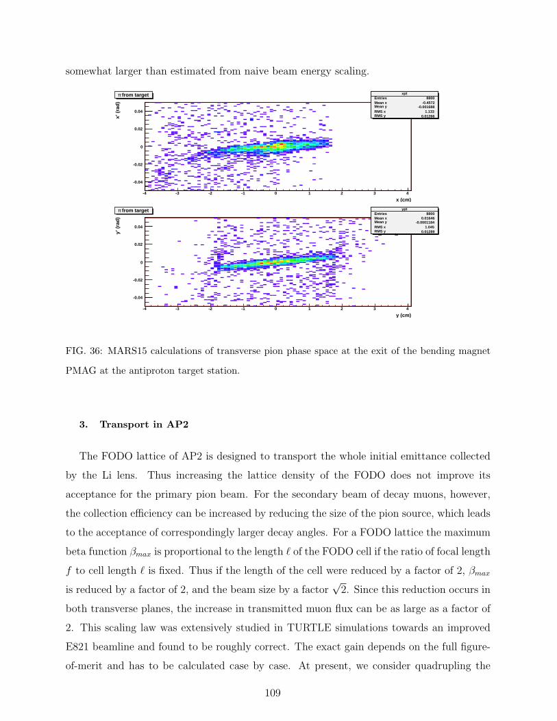
somewhat larger than estimated from naive beam energy scaling.
x (cm)-4 -3 -2 -1 0 1 2 3 4
x’ (
rad
)
-0.04
-0.02
0
0.02
0.04
xptEntries 8800Mean x -0.4572Mean y -0.001688RMS x 1.133RMS y 0.01266
xptEntries 8800Mean x -0.4572Mean y -0.001688RMS x 1.133RMS y 0.01266
from targetπ
y (cm)-4 -3 -2 -1 0 1 2 3 4
y’ (
rad
)
-0.04
-0.02
0
0.02
0.04
yptEntries 8800Mean x 0.01646Mean y -0.0001184RMS x 1.045RMS y 0.01289
yptEntries 8800Mean x 0.01646Mean y -0.0001184RMS x 1.045RMS y 0.01289
from targetπ
FIG. 36: MARS15 calculations of transverse pion phase space at the exit of the bending magnet
PMAG at the antiproton target station.
3. Transport in AP2
The FODO lattice of AP2 is designed to transport the whole initial emittance collected
by the Li lens. Thus increasing the lattice density of the FODO does not improve its
acceptance for the primary pion beam. For the secondary beam of decay muons, however,
the collection efficiency can be increased by reducing the size of the pion source, which leads
to the acceptance of correspondingly larger decay angles. For a FODO lattice the maximum
beta function βmax is proportional to the length ` of the FODO cell if the ratio of focal length
f to cell length ` is fixed. Thus if the length of the cell were reduced by a factor of 2, βmax
is reduced by a factor of 2, and the beam size by a factor√
2. Since this reduction occurs in
both transverse planes, the increase in transmitted muon flux can be as large as a factor of
2. This scaling law was extensively studied in TURTLE simulations towards an improved
E821 beamline and found to be roughly correct. The exact gain depends on the full figure-
of-merit and has to be calculated case by case. At present, we consider quadrupling the
109

lattice density of the present AP2 beamline with cost effective permanent quadrupoles and
elements of the existing E821 beamline. Pending further optimization studies, a reduction
of the magnet spacing from presently 13 m to 3.25 m in the first part of the AP2 could
increase the stored muon fraction by a factor of 1.8 compared to E821.
4. Performance Estimate
Fig. 37 sketches the basic figure of merit of the anticipated beamlines for the new FNAL
versus the previous BNL experiment. Particle numbers per 1012 protons (Tp) are presented
as a function of the assumed beamline length. The pion curve indicates the number of pions
entering the (g − 2) ring and generating the hadronic background flash. The muon curves
denote the number of stored muons. The advantage of the FNAL set-up is evident. The
significantly longer decay channel together with other beam transport improvements allows
the collection of 6 times more muons at the experimental location. The number of pions
per Tp is also reduced. The quantity relevant for the flash related background problem is
the number of pions per fill, which is smaller by another factor of four due to the higher fill
repetition rates at FNAL.
110
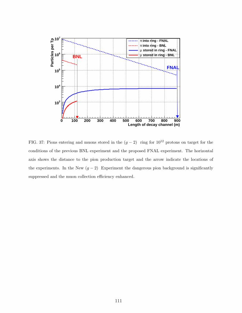
Length of decay channel (m)0 100 200 300 400 500 600 700 800 900
Par
ticl
es p
er T
p
310
410
510
610
710 into ring - FNALπ into ring - BNLπ stored in ring - FNALµ stored in ring - BNLµBNL
FNAL
FIG. 37: Pions entering and muons stored in the (g − 2) ring for 1012 protons on target for the
conditions of the previous BNL experiment and the proposed FNAL experiment. The horizontal
axis shows the distance to the pion production target and the arrow indicate the locations of
the experiments. In the New (g − 2) Experiment the dangerous pion background is significantly
suppressed and the muon collection efficiency enhanced.
111

APPENDIX B: BEAM DYNAMICS AND SCRAPING
1. The Kicker and Quadrupoles
The incoming bunched beam from the AGS is kicked on orbit by a fast muon kicker
consisting of three identical pulse-forming networks and kicker magnets. [73] The fast muon
kicker worked adequately during the running period of E821, but there are several mainte-
nance items which must be attended to. The first kicker unit must be repaired to replace a
cracked ceramic insulator, which prevented it from holding full voltage. We are also study-
ing the absolute injection efficiency to see if an additional kicker module might improve the
reliability and efficiency of injection. The rate calculations in this proposal do not assume
any additional factor from the kicker.
The electrostatic quadrupoles, which provide the (weak) vertical focusing in the storage
ring, worked well in E821. We do need to improve the lead geometry inside of the vacuum
chamber to further reduce trapped electrons, as well as improve the lead configuration
outside of the vacuum chamber where the high voltage feed-throughs are located to make
them more reliable. These changes represent modest improvements and will not be discussed
further in this proposal.
2. Beam Dynamics in the Ring
The storage ring is a weak focusing ring, with the field index n < 1.0 determined by the
strength of the electrostatic quadrupole field. In the limit of a continuous quadrupole field,
the stored muons execute simple harmonic motion radially (x) and vertically (y) with the
frequencies given by
fy = fC
√n ' 0.37fC ; fx = fC
√1− n ' 0.929fC , (B1)
where fC is the cyclotron frequency, and the field index n is given by
n =κR0
βB0
. (B2)
The numerical values are for n = 0.137. The frequencies in the ring are given in Table X.
One of the systematic errors which must be improved in the new experiment comes
from muon losses out of the storage ring which result from processes other than muon
112

Quantity Expression Frequency Period
fae
2πmcaµB 0.23 MHz 4.37 µs
fcv
2πR06.7 MHz 149 ns
fx
√1− nfc 6.23 MHz 160 ns
fy√
nfc 2.48 MHz 402 ns
fCBO fc − fx 0.477 MHz 2.10 µs
fVW fc − 2fy 1.74 MHz 0.574 µs
TABLE X: Frequencies in the (g − 2) ring. CBO = coherent betatron oscillation; V W =vertical
waist; a, c refer to spin precession ωa and cyclotron frequencies respectively.
decay. In E821 we reduced these losses by scraping off particles on the edge of the storage
volume. Scraping is defined as the creation of a gap of several mm between the beam
and the collimators that will either eliminate altogether or drastically reduce particle losses
during data collection time. This was achieved by asymmetrically powering the electrostatic
quadrupoles during and after injection for 10-15 µs and scraping the beam on collimators
placed around the ring. This asymmetry caused the beam to be lifted and moved sideways
during this scraping time. At the end of the scraping period, the beam was returned to the
equilibrium orbit with a 5 µs time constant. While losses were reduced from 0.6% per muon
lifetime in the ring with no scraping to 0.2% with scraping, we will need to do better in the
new experiment.
Because of the small inflector size relative to the storage volume, shown in Fig. 38, the
phase space in the ring is not uniformly filled. This causes the bunched beam to oscillate
coherently both vertically and horizontally in the storage ring. For a detector at a fixed point
in azimuth, the apparent radial motion of the beam is the difference frequency between the
cyclotron frequency and the horizontal betatron frequency given in Eq. B1. The inflector
image is re-formed every betatron wavelength, so that this “waist” in the beam also moves
around the ring with the difference frequency between the the cyclotron frequency and
twice the radial (vertical) betatron frequency. Since the detector acceptance depends on the
radial position of the muon when it decays, the coherent radial betatron oscillations (CBO)
amplitude-modulate the time spectrum. The modulation effect decreases in the time due to
113

(a) (b)
FIG. 38: (a) The geometry of the inflector exit and the muon storage volume. (b) The cross section
of the inflector.
the “natural” chromaticity of the betatron oscillations, which slightly mix up phases of the
particle oscillations. In E821 we measured a decoherence time of about 100 µs for the CBO,
and the muon lifetime was 64.4 µs .
In the new experiment we wish to reduce the CBO effects, and to improve the scraping
of the beam. Two approaches to reduce the coherent betatron motion and scrape the beam
have been proposed:
1. Using a RF dipole field during the time immediately after injection to first drive the
coherent betatron oscillations to scrape the beam, and then to reverse the phase to
damp the CBO. This technique would get rid of the main CBO but not the “waist”
motion in the beam.
2. A scheme which causes a fast phase mixing in the betatron tune through the intro-
duction into the machine lattice of a nonlinear focusing element such as an octupole.
Preliminary studies indicate that the CBO modulation can be minimized by applying
this field during less than a hundred turns after injection. This will also serve the
purpose of scraping the beam simultaneously with the CBO decoherence.
114
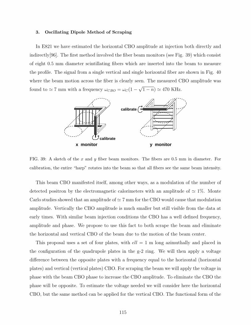
3. Oscillating Dipole Method of Scraping
In E821 we have estimated the horizontal CBO amplitude at injection both directly and
indirectly[96]. The first method involved the fiber beam monitors (see Fig. 39) which consist
of eight 0.5 mm diameter scintillating fibers which are inserted into the beam to measure
the profile. The signal from a single vertical and single horizontal fiber are shown in Fig. 40
where the beam motion across the fiber is clearly seen. The measured CBO amplitude was
found to ' 7 mm with a frequency ωCBO = ωC(1−√1− n) ' 470 KHz.
x monitor y monitor
calibrate
calibrate
FIG. 39: A sketch of the x and y fiber beam monitors. The fibers are 0.5 mm in diameter. For
calibration, the entire “harp” rotates into the beam so that all fibers see the same beam intensity.
This beam CBO manifested itself, among other ways, as a modulation of the number of
detected positron by the electromagnetic calorimeters with an amplitude of ' 1%. Monte
Carlo studies showed that an amplitude of' 7 mm for the CBO would cause that modulation
amplitude. Vertically the CBO amplitude is much smaller but still visible from the data at
early times. With similar beam injection conditions the CBO has a well defined frequency,
amplitude and phase. We propose to use this fact to both scrape the beam and eliminate
the horizontal and vertical CBO of the beam due to the motion of the beam center.
This proposal uses a set of four plates, with ell = 1 m long azimuthally and placed in
the configuration of the quadrupole plates in the g-2 ring. We will then apply a voltage
difference between the opposite plates with a frequency equal to the horizontal (horizontal
plates) and vertical (vertical plates) CBO. For scraping the beam we will apply the voltage in
phase with the beam CBO phase to increase the CBO amplitude. To eliminate the CBO the
phase will be opposite. To estimate the voltage needed we will consider here the horizontal
CBO, but the same method can be applied for the vertical CBO. The functional form of the
115
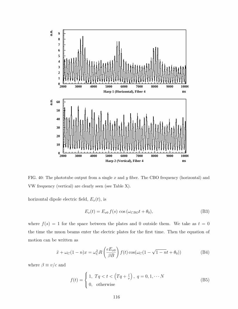
Harp 1 (Horizontal), Fiber 4 ns
a.u.
Harp 2 (Vertical), Fiber 4 ns
a.u.
0
1
2
3
4
5
6
7
8
9
2000 3000 4000 5000 6000 7000 8000 9000 10000
0
10
20
30
40
50
60
2000 3000 4000 5000 6000 7000 8000 9000 10000
FIG. 40: The phototube output from a single x and y fiber. The CBO frequency (horizontal) and
VW frequency (vertical) are clearly seen (see Table X).
horizontal dipole electric field, Ex(t), is
Ex(t) = Ex0 f(s) cos (ωCBOt + θ0), (B3)
where f(s) = 1 for the space between the plates and 0 outside them. We take as t = 0
the time the muon beams enter the electric plates for the first time. Then the equation of
motion can be written as
x + ωC(1− n)x = ω2CR
(eEx0
βB
)f(t) cos(ωC(1−√1− nt + θ0)) (B4)
where β ≡ v/c and
f(t) =
1, T q < t <(Tq + l
ν
), q = 0, 1, · · ·N
0, otherwise(B5)
116

Where T ' 149 ns, the cyclotron period of the ring. The exact solution of equation 3
with f(t) given by Eq. B5 is
x = a(t)eiωxt + a∗(t)e−iωxt (B6)
a = a0 − ieiθ0N + 1
4√
1− n
(Ex0l
βB
) [1 +
ei2θ0 [1− e−i2ωC(1−√1−nT (N+1))]
N + 1[1− e−i2ωC(1−√1−n)T ]
]. (B7)
where a0 = (xmax/2)eiα corresponds to t = 0 and defines the electric field phase θ0. After
N + 1 turns we get Eq. B7 which for large N > 10 simplifies to
a = a0 − ieiθ0N + 1
4√
1− n
(Ex0l
βB
), (B8)
where B is the storage ring dipole magnetic field. For xmax = 0.7 mm, N = 60 (i.e. about
10 µs), n = 0.142, and B = 1.45 T we need Ex0 ' 0.9 kV/cm at the CBO frequency of
' 470 KHz. For a plate separation of 10 cm it means a voltage amplitude of ' 9 KV across
the opposite plates horizontally driven at 470KHz, which is quite reasonable.
The expected beam losses after scraping the beam are going to be dominated by the
vertical scraping since it is expected that horizontally we wouldn’t need to scrape more than
' 7 mm oscillation of the beam at injection. Horizontally we would therefore just wait of
the order of 5µs for the beam to scrape off the collimators after which we would apply the
voltage estimated above to eliminate it. Vertically we would need to apply a voltage for
about 5 µs after injection in phase with the natural one so that we induce an overall vertical
oscillation of the order of 5 mm after which we will flip the sign of the phase to eliminate it.
The total beam losses induced by this method of scraping for a beam gap of 5 mm vertically
and 7 mm horizontally are estimated to be less than 20%.
4. Pulsed Octupole Method to Remove the CBO
This method effects a fast phase mixing by an introduction of a nonlinear focusing element
in the machine lattice[97]. The nonlinearity induces a dependence of betatron tunes on
amplitudes of transverse oscillations ( δQδa2 ).[98] The CBO modulation could be minimized
during a few tens of turns in the storage ring. Using a time (up to 100 turns) to apply a
pulsed closed orbit distortion can make the CBO vanish while simultaneously scraping the
beam.
117
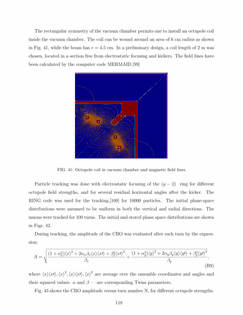
The rectangular symmetry of the vacuum chamber permits one to install an octupole coil
inside the vacuum chamber. The coil can be wound around an area of 6 cm radius as shown
in Fig. 41, while the beam has r = 4.5 cm. In a preliminary design, a coil length of 2 m was
chosen, located in a section free from electrostatic focusing and kickers. The field lines have
been calculated by the computer code MERMAID.[99]
FIG. 41: Octupole coil in vacuum chamber and magnetic field lines
Particle tracking was done with electrostatic focusing of the (g − 2) ring for different
octupole field strengths, and for several residual horizontal angles after the kicker. The
RING code was used for the tracking,[100] for 10000 particles. The initial phase-space
distributions were assumed to be uniform in both the vertical and radial directions. The
muons were tracked for 100 turns. The initial and stored phase space distributions are shown
in Figs. 42.
During tracking, the amplitude of the CBO was evaluated after each turn by the expres-
sion:
A =
√√√√(1 + α2x)〈x〉2 + 2αxβx〈x〉〈x′〉+ β2
x〈x′〉2βx
+(1 + α2
y)〈y〉2 + 2αyβy〈y〉〈y′〉+ β2y〈y′〉2
βy
,
(B9)
where 〈x〉〈x′〉, 〈x〉2, 〈x〉〈x′〉, 〈x〉2 are average over the ensemble coordinates and angles and
their squared values. α and β — are corresponding Twiss parameters.
Fig. 43 shows the CBO amplitude versus turn number N, for different octupole strengths.
118
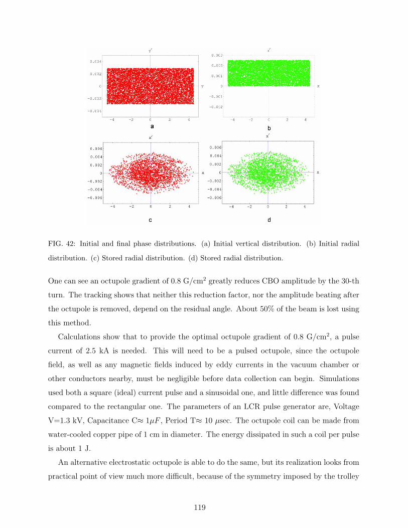
FIG. 42: Initial and final phase distributions. (a) Initial vertical distribution. (b) Initial radial
distribution. (c) Stored radial distribution. (d) Stored radial distribution.
One can see an octupole gradient of 0.8 G/cm2 greatly reduces CBO amplitude by the 30-th
turn. The tracking shows that neither this reduction factor, nor the amplitude beating after
the octupole is removed, depend on the residual angle. About 50% of the beam is lost using
this method.
Calculations show that to provide the optimal octupole gradient of 0.8 G/cm2, a pulse
current of 2.5 kA is needed. This will need to be a pulsed octupole, since the octupole
field, as well as any magnetic fields induced by eddy currents in the vacuum chamber or
other conductors nearby, must be negligible before data collection can begin. Simulations
used both a square (ideal) current pulse and a sinusoidal one, and little difference was found
compared to the rectangular one. The parameters of an LCR pulse generator are, Voltage
V=1.3 kV, Capacitance C≈ 1µF , Period T≈ 10 µsec. The octupole coil can be made from
water-cooled copper pipe of 1 cm in diameter. The energy dissipated in such a coil per pulse
is about 1 J.
An alternative electrostatic octupole is able to do the same, but its realization looks from
practical point of view much more difficult, because of the symmetry imposed by the trolley
119

FIG. 43: Behavior of the CBO amplitude as a function of turn number and octupole strength.
rails which go all the way around inside the vacuum chamber with four-fold symmetry.
120
APPENDIX C: NEW CALORIMETERS
The basic material design requirements for a new calorimeter are largely unchanged; it
must be dense and fast. Additionally, the new calorimeter must be segmented transversely
with respect to the incoming positron, so that simultaneous events can be distinguished 4
out of 5 times. Building new Pb/SciFi calorimeters with fibers running longitudinally (i.e.,
rotated by 90 degrees) is one possible solution. The downstream face of the detector would
be a fiber / lead grid that could be readout in small and independent segments. Members of
our Collaboration have built detectors of this type in the past, with incoming photons nearly
co-linear with the fiber direction. This re-oriented Pb/SciFi option is attractive in principle,
but there are two drawbacks. First, the downstream space is limited by the existing vacuum
chamber structures. A denser detector is desired to open up additional space for the readout
system. Second, simple simulations using ρM = 2.5 cm and the requirement that showers
be separated by at least 2ρM , indicate a pileup separation factor of no better than 3 (the
simulation uses the actual distribution of positrons on the calorimeter face, see Fig. 44).
The goal of the new detectors is to separate simultaneous showers by a factor of about 5.
To do so requires the detector to have a smaller Moliere radius.
We have designed and built a simple detector made of alternating layers of 0.5-mm thick
tungsten (W) plate and 0.5-mm-diameter plastic scintillator fiber ribbons. A NIM paper
is in press at the time of this writing [15]. We briefly summarize some of the interesting
findings from our studies.
The prototype module is 4× 6× 17 cm3. The calculated radiation length is 0.69 cm and
the Moliere radius is 1.7 cm. Both are much smaller than the Pb/SciFi design used in E821.
The fiber ribbons are oriented vertically so that the positrons, which are curling inward, must
cross W layers and initiate showers. The full sized detector will be made as one monolithic
structure with dimension 15 cm high by 21-cm radial. The 11-cm depth represents more than
15 X0. Fibers will be either gathered into small bundles on the downstream side forming
individual “segments” or a direct array of lightguide couplers will be attached to provide
the segmentation. At the present time, we are exploring either a 5 × 7 array of 3 × 3 cm2
segments or, with slight overall dimension changes to the SciFi block, a coarser array of
4×5 segments with front faces of 4×4 cm2. Either segmentation will easily meet our design
specifications related to pileup reduction.
121

cm0 2 4 6 8 10 12 14 16 18 20
0
500
1000
1500
2000
2500
3000
3500
4000
4500
cm-8 -6 -4 -2 0 2 4 6 8
0
1000
2000
3000
4000
5000
6000
7000
100
200
300
400
500
cm0 2 4 6 8 10 12 14 16 18 20
cm
-8
-6
-4
-2
0
2
4
6
8
FIG. 44: Right panel: Hit position of positrons on calorimeter front face from from GEANT sim-
ulation. Top left panel: radial distribution; storage ring edge is at large x values. Bottom left:
vertical distribution.
The prototype is shown in Fig. 45a. The full conceptual design array of 4 × 4 × 11 cm3
modules is shown in Fig. 45b; 24 such arrays are required for the proposed muon (g − 2)
experiment.
We have developed a simple and effective assembly procedure for these modules that
will assure consistent uniformity of the completed modules. Quotes [101, 102] have been
obtained for the fiber ribbons and flat tungsten plates, required for the full production of
24 calorimeter modules. The total cost of the calorimeter modules just under $0.5M, with
construction by the technicians at Illinois.
The prototype used 0.5-mm diameter BCF-20, “green-emitting” scintillating fibers ob-
tained from Saint-Gobain Crystals [101]. These fibers were conveniently available owing to
a large production for an independent project. They arrived as 12-cm wide by 17.5-cm long
“ribbons.” Each ribbon came as a self-contained structure with the individual 0.5-mm fibers
held adjacent by a coating of a polyurethane-acrylic blend cement. We split each ribbon
into two 6-cm wide strips to match the tungsten plate widths. The fibers are coated with
a 10 − 15 µm thick white extra mural absorber for better light transmission. For the final
122

(a)Prototype module and guide (b)Proposed array of 20 modules
FIG. 45: a) Prototype 4 × 6 × 17 cm3 module and b) proposed array of twenty 4 × 4 × 11 cm3
modules. The lightguides must curl toward the (g − 2) storage ring center and connect to PMTs
outside of the storage ring magnetic field.
production modules, BCF-10 (or equivalent) “blue” fibers will be used to better match the
quantum efficiency of the readout device and for faster time response.
The W/SciFi detector was first tested at the Paul Scherrer Institut (PSI) and at the
Meson Test Beam at Fermilab. The focus of the test beam measurements was on calorime-
ter linearity and energy resolution. While neither beamline was optimized to provide a
small momentum resolution or spot size, sufficient performance information was obtained to
compare measurement to GEANT-4 based Monte Carlo simulations.
The typical (g − 2) energy threshold for including events is 1.8 − 2 GeV; positrons are
only accepted above this threshold. A resolution of ∼ 10% (defined as σ/E for a simple
Gaussian fit) would give an acceptable performance for this threshold in a future (g − 2)
experiment. The response of the prototype tungsten detector is shown in Fig. 46 for 2 GeV
electrons impacting at 5 degrees with respect to the fiber axis. An entrance cut is made
using beamline wire chamber information to select the central 15 mm by 30 mm (width by
height) of the 40- by 60-mm detector face. Even with no corrections for leakage into side
detectors, or adjustments for sub-optimal light collection, or beam momentum uncertainty,
the resolution at 10.1± 0.3% meets the experimental goal.
Our goal is to understand the intrinsic sampling resolution of this detector and compare it
to simulation. While the stochastic term is mainly determined by the sampling fluctuations
123

intrinsic to the active-to-absorber material ratio and the effective layer thickness, additional
contributions enter from photo-statistics. A 5% contribution exists from photo-statistics,
because the measured photoelectron (pe) yield is 400 pe/GeV. This is a smaller light yield
than we would expect had the lightguide been better matched in area to the photomultiplier
tube and if blue fibers were used instead of green (higher quantum efficiency). Two factors
that scale with energy contribute to energy degradation—the transverse leakage, and the
momentum uncertainty of the test beam. The leakage can be explored with data cuts and
simulation; the ∆P/P is unknown but estimated to be a few percent. In Fig. 47, we plot
the FNAL data fit toσ(E)
E=
√A2 + ∆2
pe
E+ B2. (C1)
Here A/√
E represents the intrinsic sampling term, ∆pe/√
E is the photo-statistics uncer-
tainty, and B is a linear term. The term ∆pe is fixed at 5% and E is given in GeV. The
upper curve is a fit based on data where a 25 mm “wide cut” in the entrance width of the
beam was used, while the lower curve is a fit based on a 5 mm “narrow cut.” The change
affects both the sampling and the constant term as they are not easily separable, given the
statistics. The narrow cut result minimizes, but does not eliminate, the leakage, resulting
in Ameas = 11.8 ± 1.1% and Bmeas = 3.7 ± 1.3% for the stochastic and constant terms,
respectively.
The sampling fluctuation component can be predicted using a complete GEANT-4 model.
A plot of this resolution versus energy for simulated electrons impacting on the module
center at a 5-degree angle is shown in Fig. 48. Three curves are presented representing a
high-statistics “pencil beam” with a 1 mm spot size in both dimensions, as well a separate
simulation with data-like cuts of 5- and 25-mm entrance widths, which match the narrow
and wide definitions for the data. The most appropriate comparison to data is the narrow
cut, which yields Asim = 10.6± 0.8% and Bsim = 2.9± 1.1% for the stochastic and constant
terms, respectively. The B term is representative of the leakage, since no ∆P/P uncertainty
contributes for Monte Carlo. If we deconvolute the leakage contribution from the B term in
the data, a ∆P/P of ≈ 2.3% is implied, which is not unreasonable.
The simulation is, not surprisingly, somewhat better than the actual prototype—Asim =
10.6±0.8% vs. Ameas = 11.8±1.1%. Detector construction imperfections can contribute, as
would non-uniform light collection in the guide. However, to explore this comparison more
124

/ ndf = 35.96 / 362χAmp 2.24± 49.45
Mean 0.8± 209.3 Sigma 0.72± 21.11
Channels100 150 200 250 300
Co
un
ts
0
10
20
30
40
50
60 / ndf = 35.96 / 362χAmp 2.24± 49.45
Mean 0.8± 209.3 Sigma 0.72± 21.11
FIG. 46: Example raw W/SciFi detector ADC data for a 2 GeV electron beam impacting at a 5
degree incidence. A modest containment cut of 15 mm width is made.
completely will require a larger test module with improved readout and a better controlled
test beam environment. Note, that we carefully checked the GEANT-4 cut parameters, but
found no dependence on them that altered our results.
Based on these studies, we intend to build a larger prototype that allows for full shower
containment and readout by multiple optical devices. We are considering two options. The
conservative plan is to use 29-mm (1-1/8 in) PMTs whose basic characteristics are under-
stood and standard. We are using an array of 340 Photonis XP-2982, 11-stage PMTs for the
muon lifetime experiment MuLan at PSI. The similar 10-stage XP-2972 is more appropriate
for the New (g−2) Experiment because of the high light yield from the calorimeter modules.
Both tubes were carefully evaluated by us and feature similar important characteristics: low
noise, high gain, no detectable after-pulses. We will have to design a robust, rate-dependent
base as the initial rate of up to a few MHz is higher than what can be comfortably handled
by the stock resistor divider network in the simplest Photonis bases. For E821, we developed
a gated base that allowed the PMT to be “turned off” during injection and turned back
on within 1 µs after injection. Depending on the level of hadronic flash, we may need to
incorporate this gating feature—therefore, we will plan to do so in our design.
The rapid development of silicon photomultiplier tubes (SiPMs) and their packaging
125

/ ndf 2χ 7.767 / 3Percent 0.57± 12.78 Constant 0.646± 4.521
Energy (GeV)1.5 2 2.5 3 3.5
Sig
ma
/ Mea
n (
%)
7
8
9
10
11
12
13 / ndf 2χ 7.767 / 3
Percent 0.57± 12.78 Constant 0.646± 4.521
/ ndf 2χ 3.93 / 3Percent 1.08± 11.78 Constant 1.339± 3.733
Wide cut
Narrow cut
FIG. 47: Measured resolution at 5-degree impact angle versus energy. The upper curve (dotted) is
a fit to data obtained requiring a 25-mm-wide entrance cut. The lower curve (solid) is a fit to data
obtained using a 5-mm-wide entrance cut. The“Percent” term represents the intrinsic sampling
term (A in the text); a 5% photo-statistics stochastic term has been removed in the fit function.
into relatively large arrays is very attractive. These SiPMs are very fast and they can be
mounted onboard, in the magnetic field, thus avoiding the costly and clumsy development
of lightguides and external housing. We are adopting this as our baseline, given the time
we have to develop this technique together with several of our new collaborators who have
expertise in this field.
126

/ ndf 2χ 3.119 / 3Percent 0.37± 11.33 Constant 0.436± 3.796
Energy (GeV)1.5 2 2.5 3 3.5
Sig
ma(
E)/
E
5
6
7
8
9
10
11 / ndf 2χ 3.119 / 3Percent 0.37± 11.33 Constant 0.436± 3.796
/ ndf 2χ 1.667 / 2Percent 0.500± 9.496 Constant 0.971± 2.105
/ ndf 2χ 7.87 / 3Percent 0.79± 10.59 Constant 1.14± 2.88
Wide cut
Narrow cut
Pencil beam
FIG. 48: Fits to resolution versus energy in the central module of an array of W/SciFi modules.
Three entrance width cuts are imposed: 25 mm (dotted), 5 mm (dashed), and 1 mm “pencil”
(solid).
127

FIG. 49: Plan view of new calorimeter in the region of the bellows between vacuum chambers
where the available space for lightguides is quite restricted.
128