the nature of the trappist-1 exoplanets

Astronomy & Astrophysics manuscript no. trappist1 c©ESO 2018January 31, 2018

The nature of the TRAPPIST-1 exoplanetsSimon L. Grimm1, Brice-Olivier Demory1, Michaël Gillon2, Caroline Dorn1,19, Eric Agol3,4,17,18, Artem Burdanov2,

Laetitia Delrez5,2, Marko Sestovic1, Amaury H.M.J. Triaud6,7, Martin Turbet8, Émeline Bolmont9, Anthony Caldas10,Julien de Wit11, Emmanuël Jehin2, Jérémy Leconte10, Sean N. Raymond10, Valérie Van Grootel2, Adam J. Burgasser12,

Sean Carey13, Daniel Fabrycky14, Kevin Heng1, David M. Hernandez15, James G. Ingalls13, Susan Lederer16,Franck Selsis10, Didier Queloz5

1 University of Bern, Center for Space and Habitability, Gesellschaftsstrasse 6, CH-3012, Bern, Switzerland2 Space Sciences, Technologies and Astrophysics Research (STAR) Institute, Université de Lège, Allée du 6 Août 19C, B-4000Liège, Belgium3 Astronomy Department, University of Washington, Seattle, WA, 98195, USA4 NASA Astrobiology Institute’s Virtual Planetary Laboratory, Seattle, WA, 98195, USA5 Cavendish Laboratory, J J Thomson Avenue, Cambridge, CB3 0HE, UK6 Institute of Astronomy, Madingley Road, Cambridge CB3 0HA, UK7 School of Physics & Astronomy, University of Birmingham, Edgbaston, Birmingham B15 2TT, United Kingdom.8 Laboratoire de Météorologie Dynamique, IPSL, Sorbonne Universités, UPMC Univ Paris 06, CNRS, 4 place Jussieu, 75005 Paris,France9 Université Paris Diderot, AIM, Sorbonne Paris Cité, CEA, CNRS, F-91191 Gif-sur-Yvette, France.10 Laboratoire d’astrophysique de Bordeaux, Univ. Bordeaux, CNRS, B18N, allée Geoffroy Saint-Hilaire, 33615 Pessac, France11 Department of Earth, Atmospheric and Planetary Sciences, Massachusetts Institute of Technology, 77 Massachusetts Avenue,Cambridge, MA 02139, USA12 Center for Astrophysics and Space Science, University of California San Diego, La Jolla, CA, 92093, USA13 IPAC, Mail Code 314-6, Calif. Inst. of Technology, 1200 E California Blvd, Pasadena, CA 91125, USA14 Department of Astronomy and Astrophysics, Univ. of Chicago, 5640 S Ellis Ave, Chicago, IL 60637, USA15 Department of Physics and Kavli Institute for Astrophysics and Space Research, Massachusetts Institute of Technology, 77Massachusetts Ave., Cambridge, Massachusetts 02139, USA16 NASA Johnson Space Center, 2101 NASA Parkway, Houston, Texas, 77058, USA17 Guggenheim Fellow18 Institut d’Astrophysique de Paris, 98 bis bd Arago, F-75014 Paris, France19 University of Zurich, Institute of Computational Sciences, Winterthurerstrasse 190, CH-8057, Zurich, Switzerland

Received

ABSTRACT

Context. The TRAPPIST-1 system hosts seven Earth-sized, temperate exoplanets orbiting an ultra-cool dwarf star. As such, it rep-resents a remarkable setting to study the formation and evolution of terrestrial planets that formed in the same protoplanetary disk.While the sizes of the TRAPPIST-1 planets are all known to better than 5% precision, their densities have significant uncertainties(between 28% and 95%) because of poor constraints on the planet’s masses.Aims. The goal of this paper is to improve our knowledge of the TRAPPIST-1 planetary masses and densities using transit-timingvariations (TTV). The complexity of the TTV inversion problem is known to be particularly acute in multi-planetary systems (con-vergence issues, degeneracies and size of the parameter space), especially for resonant chain systems such as TRAPPIST-1.Methods. To overcome these challenges, we have used a novel method that employs a genetic algorithm coupled to a full N-bodyintegrator that we applied to a set of 284 individual transit timings. This approach enables us to efficiently explore the parameter spaceand to derive reliable masses and densities from TTVs for all seven planets.Results. Our new masses result in a five- to eight-fold improvement on the planetary density uncertainties, with precisions rang-ing from 5% to 12%. These updated values provide new insights into the bulk structure of the TRAPPIST-1 planets. We find thatTRAPPIST-1 c and e likely have largely rocky interiors, while planets b, d, f, g, and h require envelopes of volatiles in the form ofthick atmospheres, oceans, or ice, in most cases with water mass fractions less than 5%.

Key words. Planets and satellites – Techniques: photometric – Methods: numerical

1. Introduction

The TRAPPIST-1 system, which harbours seven Earth-size ex-oplanets orbiting an ultra-cool star (Gillon et al. 2017), repre-sents a fascinating setting to study the formation and evolutionof tightly-packed small planet systems. While the TRAPPIST-1

planet sizes are all known to better than 5%, their densities suf-fer from significant uncertainty (between 28 and 95%) becauseof loose constraints on planet masses. This critically impacts inturn our knowledge of the planetary interiors, formation path-way (Ormel et al. 2017; Unterborn et al. 2017) and long-termstability of the system. So far, most exoplanet masses have been

Article number, page 1 of 24

A&A proofs: manuscript no. trappist1

measured using the radial-velocity technique. But because ofthe TRAPPIST-1 faintness (V=19), precise constraints on Earth-mass planets are beyond the reach of existing spectrographs.

Thankfully, the resonant chain formed by the planetary septet(Luger et al. 2017) dramatically increases the exchange of torqueat each planet conjunction, resulting in transit timing variations(TTV) (Holman 2005; Agol et al. 2005) that are well above ourdemonstrated noise limit for this system. Presently, the TTV ap-proach thus represents the only avenue to characterise the phys-ical properties of the system. The TRAPPIST-1 system showsdynamical similarities to Kepler-90 system (Cabrera et al. 2014)which contains also seven planets and resonances conditions be-tween pairs of the them.

Planetary masses published in the TRAPPIST-1 discoverypaper (Gillon et al. 2017) were bearing conservative uncertain-ties because the different techniques used by the authors sug-gested a non-monotonous parameter space with the absence ofa single global minimum. Subsequent studies have adequatelyinvoked the requirement for long-term stability to refine thesemasses further (Quarles et al. 2017; Tamayo et al. 2017a), butthe parameter space allowed by this additional constraint maystill be too large to precisely identify the planet physical prop-erties. The recent K2 observations of TRAPPIST-1 (Luger et al.2017) enabled another team to compute updated masses for thesystem using the K2 data combined to archival data (Wang et al.2017). Their approach relies on the TTVFast algorithm (Decket al. 2014), which uses low-order symplectic co-ordinates andan approximate scheme for finding transit times to increase effi-ciency. It is however unclear from that paper how the correlationsbetween parameters are taken into account and how comprehen-sive the search of the parameter space is. Only a full benchmark-ing of this approach with more accurate integrators for this spe-cific system could validate their results.

In the present paper, we have used a novel approach thatcombines an efficient exploration of the parameter space basedon a genetic algorithm with an accurate N-body integrationscheme. The associated complexity being compensated by morecomputing resources. The philosophy of this approach could beconsidered ‘brute force’but still represents a useful avenue to ap-preciate the degeneracy of the problem without doubting the ac-curacy of the numerical integration scheme.

2. Observations

2.1. Published data

This study is based on 284 transit timings obtained betweenSeptember 17, 2015 and March 27, 2017 through the TRAP-PIST and SPECULOOS collaboration. The input data for ourtransit-timing analysis includes 107 transits of planet b, 72 of c,35 of d, 28 of e, 19 of f, 16 of g and 7 of h. In addition to theTRAPPIST-1 transit timings already presented in the literature(Gillon et al. 2016, 2017; de Wit et al. 2016; Luger et al. 2017),we have included new data from the Spitzer Space Telescope(PID 12126, 12130 and 13067) and from Kepler and K2 (PID12046). Transit timing uncertainties range from 8 sec to 6.5 minwith a median precision across our dataset of 55 sec. The analy-sis of the K2 data is presented below while the new Spitzer dataobtained between February and March 2017 are presented in aseparate publication (Delrez et al. 2018). We include the full listof transit timings used in this work in Tables A.1 through A.10of Appendix A.

2.2. K2 short-cadence photometry

For the purpose of this analysis we have included the transit tim-ings derived from the K2 photometry (Howell et al. 2014), whichobserved TRAPPIST-1 during Campaign 12 (Luger et al. 2017).We detail in the following the data reduction of this dataset.We used the K2’s pipeline-calibrated short-cadence target pixelfiles (TPF) that includes the correct timestamps. The K2 TPFTRAPPIST-1 (EPIC ID 246199087) aperture is a 9x10 postagestamp centred on the target star, with 1-minute cadence intervals.We performed the photometric reduction by applying a centroid-ing algorithm to find the (x, y) position of the PSF centre in eachframe. We used a circular top-hat aperture, centred on the fit-ted PSF centre of each frame, to sum up the flux. We find thismethod to produce a better photometric precision compared toapertures with fixed positions.

The raw lightcurve contains significant correlated noise, pri-marily from instrumental systematics due to K2’s periodic rollangle drift and stellar variability. We have accounted for thesesystematic sources using a Gaussian-processes (GP) method, re-lying on the fact that the instrumental noise is correlated with thesatellite’s roll angle drift (and thus also the (x, y) position of thetarget) and that the stellar variability has a much longer timescalethan the transits. We used an additive kernel with separate spa-tial, time and white noise components (Aigrain et al. 2015, 2016;Luger et al. 2017):

kxy(xi, yi, x j, y j) = Axy exp− (xi − x j)2

L2x

−(yi − y j)2

L2y

(1)

kxy(ti, t j) = At exp[−

(ti − t j)2

L2t

](2)

Ki j = kxy(xi, yi, x j, y j) + kt(ti, t j) + σ2δi j, (3)

where x and y are the pixel co-ordinates of the centroid, t isthe time of the observation, and the other variables (Axy, Lx, Ly,At, Lt, σ) are hyperparameters in the GP model (Aigrain et al.2016). We used the GEORGE package (Ambikasaran et al. 2016)to implement the GP model. We used a differential evolution al-gorithm (Storn & Price 1997) followed by a local optimisationto find the maximum-likelihood hyperparameters.

We optimised the hyperparameters and detrended thelightcurve in three stages. In each stage, using the hyperparam-eter values from the previous stage (starting with manually cho-sen values), we fitted the GP regression and flag all points fur-ther than 3σ from the mean as outliers. The next GP regressionand hyperparameter optimisation is performed by excluding theoutlier values. Points in and around transits are not included inthe fit. Due to the large numbers of points in the short cadencelightcurve, only a random subset of the points is used to performeach detrending and optimisation step to render the computa-tion less intensive. We achieved a final RMS of 349 ppm per 6hours (excluding in-transit points and flares). Out of the entiredataset, we discarded only two transits because of a low SNRat the following BJDT DB: 7795.706 and 7799.721. Both eclipsescorrespond to transits of planet d.

We then used a Markov Chain Monte Carlo (MCMC) algo-rithm previously described in the literature (Gillon et al. 2012)to derive the individual transit timings of TRAPPIST-1b, c, d, e,f, g, and h from the detrended K2 light curve. Each photometricdata point is attached to a conservative error bar that accounts for


Grimm et al.: The nature of the TRAPPIST-1 exoplanets

0.06 0.04 0.02 0.00 0.02 0.04 0.06

Time from mid-transit (d)

0.88

0.90

0.92

0.94

0.96

0.98

1.00

Rela

tive b

rightn

ess

b

c

d

e

f

g

h

Fig. 1. Folded short-cadence lightcurves extracted from K2 data, cor-rected for their TTVs. For clarity, the short-cadence data are binned toproduce the coloured points, with five cadences per point. The whitepoints are further binned, with ten points taken from the folded curveper bin.

the uncertainties in the detrending process presented above. Wehave imposed normal priors in the MCMC fit on the orbital pe-riod, transit mid-time centre and impact parameter for all plan-ets to the published values (Gillon et al. 2017). We computedthe quadratic limb-darkening coefficients u1 and u2 in the Ke-pler bandpass from theoretical tables (Claret & Bloemen 2011)and employ the transit model of Mandel & Agol (2002) for ourfits. We derived the transit-timing variations directly from ourMCMC fit for all TRAPPIST-1 planets. We report the medianand 1-sigma credible intervals of the posterior distribution func-tions for the 124 K2 transit timings in Tables A.1 to A.10. Theresulting K2 short-cadence stacked light curves are shown onFigure 1.

3. Methodology

3.1. Dynamical modelling

Dynamical studies of the TRAPPIST-1 system are challengingdue to the 7-planet, Laplace resonance-chain architecture withtight pair period ratios of 8:5, 5:3, 3:2, 3:2, 4:3 and 3:2. Thisconfiguration requires computationally-expensive orbital inte-grations over a large parameter space. The observed transit timesare distributed over more than 550 days, corresponding to over370 orbits of the innermost planet b. In order to accommodate theorder of one billion time steps needed in a Markov Chain MonteCarlo (MCMC) method to match the timing precisions with thetimespan of observations, we used graphics processing units(GPUs) and the GPU N-body code GENGA (Grimm & Stadel2014). We calculated the orbits of all seven planets and deter-mine the transit timing variations (TTVs) through MCMC tech-niques. GENGA uses a hybrid symplectic integration scheme(Chambers 1999) to run many instances of planetary systemsin parallel on the same GPU. We have extended the GENGAcode by implementing a GPU version of the parallel DifferentialEvolution MCMC (DEMCMC) technique (Braak 2006; Vrugtet al. 2009). DEMCMC deploys multiple Markov chains si-multaneously that efficiently sample the highly-correlated multi-dimensional parameter space that is typical of TTV inversionproblems (Mills et al. 2016). In addition we have modified theDEMCMC sampling method, such that it works more efficientlywith the large correlations impacting the masses, semi-majoraxes and mean anomalies of the different planets.

3.2. Transit timing calculations

Following (Fabrycky 2010), we defined the X-Y plane as theplane of the sky, while planets transit in front of the star at posi-tive values of the Z co-ordinate. The mid-transit times are foundby minimising the value of the function

g(xi, xi, yi, yi)=xi xi + yiyi, (4)

which can be solved by setting the next time step of our numeri-cal integrator to

δt = −g(∂g∂t

)−1

, (5)

with

∂g∂t

= x2i + xi xi + y2

i + yiyi. (6)

The quantities xi and yi are the astrocentric co-ordinates ofthe planet i.

We used a pre-checker in the integrator to determine if a tran-sit is expected to happen during the next time step. This will hap-pen if the value of gi moves from a negative value to a positivevalue during the next time step, and if zi > 0. In addition, weused the conditions |g/g| < 3.5 ·dt and rsky < (Rstar + Ri) + |vi| ·dtto refine the pre-checker, where |rsky| = |(xi, yi)| is the radial co-ordinate on the sky plane, |vi| is the norm of the velocity, and Rithe radius of planet i; and R? the radius of the star.

Since the integration is performed with a symplectic integra-tor, the co-ordinates of the position and velocity of a planet arenot simultaneously known, which leads to a small error in thecalculation of g. If a transit occurs very close to a time step, thenit can happen that the transit is reported in both successive time



steps with a slightly different mid-transit time. But when the timestep is small enough, this error can be safely neglected. Also, inhighly eccentric orbits, the described pre-checker may not workproperly, because g changes too quickly between each time step.We thus restricted ourselves in this work to eccentricities smallerthat 0.2 and used the fourth-order integrator scheme with a timestep of 0.08 days. When the pre-checker has detected a transitcandidate, then all planets are integrated with a Bulirsh-Stoerdirect N-body method for a time step and the Eq. 5 is iterateduntil δt is smaller than a tolerance value. A transit is reported ifrsky < Rstar + Ri.

3.3. Orbital parameter search

To determine the best orbital parameters, we used a parallel dif-ferential evolution Markov Chain Monte Carlo method (DEM-CMC) (Braak 2006; Vrugt et al. 2009). We used N parallelMarkov chains, where each chain consists of a d dimensionalparameter vector xi. To update the population of N chains, eachx is updated by generating a proposal

xp = xi + γ(x j − xk) + e, (7)

with i , j, i , k, j , k, γ = 2.38√

2dand a small perturbation e. The

proposal is accepted with a probability p = min(1, π(xp)/π(xi)).When the proposal is accepted, then xi is replaced by xp in thenext generation; otherwise the state remains unchanged. In each30th generation, we set γ = 0.98 to allow jumps between mul-timodal solutions (Braak 2006). In addition, we set γ = 0.01and xi = xl,i during the burn-in phase to eliminate outliers. Al-ternatively, we also tested the affine invariant ensemble walkerMCMC method (Goodman & Weare 2010; Foreman-Mackeyet al. 2013), which yields a comparable performance.

For the probability density function, π(xi) we used

π(xi) = exp(−χ2(xi

2))

= exp

12−

∑t

(Tcalc,t − Tobs,t

σt

)2 , (8)

where the running index t refers to the transit epoch, Tcalc are thecalculated mid transit times, Tobs are the observed mid-transittimes and σ are the observation uncertainties. Using Eq. 8, werewrite the acceptance probability as

p = min[1, exp

(−χ2(xp) + χ2(xi)

2τ

)], (9)

where τ is the MCMC sampling ‘temperature’. In this work, weused values for τ between 1000 and 1. Using a large value forτ increases the acceptance probability of the next DEMCMCstep and allows the walkers to explore more easily a large pa-rameter space, but the obtained probability distribution does notcorrespond to the likelihood. Resampling the so-obtained like-lihood region with a smaller value of τ, and starting from themedian values of the previous runs, refines the sampling moreaccurately. Using different values of τ in an iterative order al-lows us to sample a large parameter space, with good accuracyin the most likely region. The median and the standard deviationare calculated with a value of τ = 1. Figure 4 shows the obtainedposterior probability distribution of the masses and eccentrici-ties. We note that using a value for τ < 1 in Eq. 9 would lead tosmaller standard deviations.

According to (Gozdziewski et al. 2016), we used the follow-ing fitting parameters for the orbital elements:

Pi = 2π

√a3

i

G(M? + mi)(10)

Ti = t +Pi

2π

(MT

i − Mi

)(11)

xi =√

ei cosωi (12)

yi =√

ei sinωi (13)mi, (14)

with the period Pi, the time of the first transit Ti, the starttime of the simulation t, the mean anomaly at the first transitMT

i , the mean anomaly Mi, the eccentricity ei, the argument ofperihelion ωi and the Jacobi mass mi for each planet i. The Ja-cobi mass of planet i includes also the masses of all objects witha smaller semi-major axis. We used the square root of the ec-centricity in the parameters xi and yi to favour low eccentricitysolutions. We set the longitude of the ascending node Ωi to zeroand the inclination of all planets to π/2, which allows us to cal-culate MT

i through the true anomaly at the transit νTi = π/2 − ωi

1.Assuming coplanarity is motivated by the fact that the stan-

dard deviation of the derived inclinations for all seven planetswith respect to the sky plane is 0.08 degrees only (Gillon et al.2017). If the longitudes of nodes were distributed randomly onthe sky, then the probability that all planets transit would be verysmall (most observers would see only one planet transit if thiswere the case). Thus, the three-dimensional mutual inclinationcan be constrained by simulating the angular momentum vectorsof the planets drawn from an 3-D Gaussian inclination distribu-tion of width σθ, allowing the density of the star to vary, ρ∗, anddetermining which set of parameters matches the transit dura-tions most precisely from observers drawn from random loca-tions on the sphere. This yields a constraint on the three dimen-sional inclination distributions of σθ < 0.3 at the 90% confi-dence level (Luger et al. 2017). Transit timing variations dependvery weakly on the mutual inclinations of the planets (Nesvorný& Vokrouhlický 2014), and since these planets are constrained tobe coplanar to a high degree based upon the argument in Lugeret al. (2017), our model is justified in neglecting mutual inclina-tions of the planets for our dynamical analysis.

As initial conditions of the DEMCMC parameter search,we have randomly distributed the parameters in the range mi ∈

[0, 6 × 10−6M], ei ∈ [0, 0.05]2, ωi ∈ [0, 2π] and Mi ∈ [0, 2π].We did not assume any priors on the parameters, but restrict theeccentricity to e < 0.2.

A difficulty in sampling the orbital parameters of TTVs is,that there can exist strong correlations between some of the pa-rameters, especially between m and a or between e and ω. Thecorrelation between m and a can be explained, because the pe-riod Pi in Eq. 10 depends on all the masses of the more innerplanets. The correlation between e and ω is caused by the res-onance configuration, and a change in one of these parametersmust be compensated by the others to get a similar time of clos-est approach between the planets. When the different walkers

1 This equation is only valid for i = 90. A discussion for the casei , 90 is given in Gimenez & Garcia-Pelayo (1983)2 Tests show that setting higher initial values of e, up to 0.2, does notchange the results. Additionally, having higher eccentricities make sucha packed planetary system very likely to be dynamically unstable. Inthe long term stability analysis in section 6.2, the eccentricities remainbelow 0.025.



of the DEMCMC method are spread out over a large region inthe parameter space, then the acceptance ratio of the DEMCMCsteps will get very low, due to inaccurate guesses of the semi-major axes and mean anomalies.

3.3.1. Sub-step optimisation

The DEMCMC algorithm generates proposal values of the pa-rameters, by linearly interpolating between two accepted values,but often the parameters in the optimisation problem show a non-linear dependency. This means that the DEMCMC approach al-ways deviates from an optimal choice of the new proposal steps.Since the value of χ2 is very sensitive to small perturbations ofthe semi-major axis and the mean anomaly, inaccurate guesseson these parameters will lead to dramatic high values of χ2, andthe proposal step is very unlikely to be accepted. The conse-quence is an acceptance ratio going towards zero as the param-eters begin to populate a broader region in the parameter space.To improve this issue, we introduced a sub-step optimisationscheme to find the optimal values for the semi-major axis a andthe mean anomaly M. The sub-step scheme is applied after eachDEMCMC step, and has to be performed for each planet in a se-rial way. When the value of a or M is changed for only a singleplanet, then the χ2 shows a parabolic behaviour, which enablesthe use of a quadratic estimator to find its optimal values x, basedon three guesses x1, x2 and x3 as follows:

x =x1 + x2

2−

b1

2b2, (15)

withb0 = y1

b1 =y2 − y1

x2 − x1

b2 =1

x3 − x2·

[y3 − y1

x3 − x1− b1

],

where x means either a or M, and y j means the values of χ2

at locations x j. The cost of the described sub-step optimisationscheme is, that three times as many walkers are needed to gen-erate the values y1, y2 and y3, and each DEMCMC step has tobe followed by 14 sub-steps of computing the TTVs to adjust aand M for each planet. But even if this scheme is expensive tocompute, it allows us to achieve an acceptance rate that remains> 20 − 30% for a much larger number of DEMCMC steps. Thebest χ2 obtained is 342, details are listed in Table 1. The evo-lution of the masses and the autocorrelation functions of 5000DEMCMC steps with the described sub-step sampling for 100chains are shown in Figure 5, which shows efficient convergenceof the chains.

3.3.2. Independent analysis

We also carried out an independent transit timing analysis with anew version of TTVFast (Deck et al. 2014) which utilises a novelsymplectic integrator based upon a fast Kepler solver (Wisdom& Hernandez 2015; Hernandez & Bertschinger 2015). The inte-grator uses a time step of 0.05 days, assumes a plane-parallel ge-ometry, and alternates between drifts and universal Kepler stepsbetween pairs of planets. A drift in Cartesian co-ordinates is de-fined as an update of some or all positions assuming constantvelocities. The initial conditions are constructed with Jacobi co-ordinates, and the integration uses Cartesian co-ordinates in a

planet Nobservations Ndo f χ2 reduced χ2

b 107 102 126.15 1.23c 72 67 101.47 1.51d 35 30 31.48 1.04e 28 23 24.44 1.06f 19 14 32.75 2.33g 16 11 21.16 1.92h 7 2 4.81 2.40

all 284 249 342.29 1.37Table 1. Number of observations, number of degrees of freedom Ndo f =Nobservations −Nparameters, χ2 from Eq. 8 and reduced χ2 = χ2/Ndo f , for allplanets separately and for all planets together.

center-of-mass frame. The transit times are found by trackingthe projected sky position and velocity, and finding when the dotproduct changes sign, using Eq. 4-6. The transit centre is foundby bracketing and interpolating the time steps (Deck et al. 2014).This yields timing precisions of better than a few seconds, whichis sufficient to model the data given the observational uncertain-ties. We modelled the transit times with this code, and obtainedidentical masses for the maximum likelihood (within the uncer-tainties) , as well as broadly consistent eccentricities. Since thisanalysis was carried out with a different code in a different lan-guage (Julia) with a different integration technique, the fact thata similar maximum a posteriori likelihood gives confidence thatwe have found a unique solution for the mass ratios of this planetsystem.

4. Results

The TTV values of 1000 MCMC posterior samples with τ =1 are shown in Figure 2, in comparison to the observed transittimes. The TTV residuals for each transit are shown in Figure 3.We compute the planet densities ρp independently from the stel-lar mass, by using the planetary radii- and mass-ratio posteriorsMp

M?and Rp

R?, along with the well constrained stellar density ρ?

determined photometrically from the Spitzer dataset (Seager &Mallén-Ornelas 2003). The planet density then is ρp = ρ?

Mp

M?

R3?

R3p

(Jontof-Hutter et al. 2014). Using the stellar density from thephotometry is valid in our case because the planets’ eccentrici-ties are found to be small. Determining planetary densities usingthis approach effectively removes any inaccuracy from the stellarmodels and improves our constraints on the planetary interiors.To transform our results into physical masses and radii, we usethe most recent stellar mass estimate of 0.089 ± 0.007 M (VanGrootel et al. 2018).

Our resulting posterior distribution functions for the massesand eccentricities for all seven planets are shown in Figure 4.To perform the search over a large parameter space, differentsampling ‘temperatures’ τ are used in an iterated order. Throughour extensive exploration of the parameter space we find thatthe masses and eccentricities for all planets are reasonably con-strained (3% - 9% for mass, and 6% - 25% for eccentricity). Ta-ble 2 summarises the planetary physical parameters (mass andradius ratios) while Table 3 displays the planets’ orbital param-eters. A full posterior distribution between all mutual pairs ofparameters is shown in Figure 6.



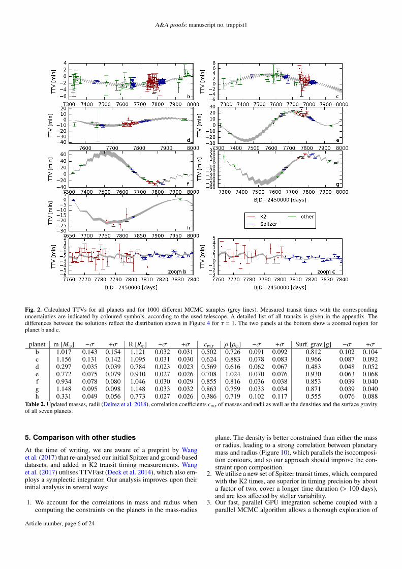
Fig. 2. Calculated TTVs for all planets and for 1000 different MCMC samples (grey lines). Measured transit times with the correspondinguncertainties are indicated by coloured symbols, according to the used telescope. A detailed list of all transits is given in the appendix. Thedifferences between the solutions reflect the distribution shown in Figure 4 for τ = 1. The two panels at the bottom show a zoomed region forplanet b and c.

planet m [M⊕] −σ +σ R [R⊕] −σ +σ cm,r ρ [ρ⊕] −σ +σ Surf. grav.[g] −σ +σb 1.017 0.143 0.154 1.121 0.032 0.031 0.502 0.726 0.091 0.092 0.812 0.102 0.104c 1.156 0.131 0.142 1.095 0.031 0.030 0.624 0.883 0.078 0.083 0.966 0.087 0.092d 0.297 0.035 0.039 0.784 0.023 0.023 0.569 0.616 0.062 0.067 0.483 0.048 0.052e 0.772 0.075 0.079 0.910 0.027 0.026 0.708 1.024 0.070 0.076 0.930 0.063 0.068f 0.934 0.078 0.080 1.046 0.030 0.029 0.855 0.816 0.036 0.038 0.853 0.039 0.040g 1.148 0.095 0.098 1.148 0.033 0.032 0.863 0.759 0.033 0.034 0.871 0.039 0.040h 0.331 0.049 0.056 0.773 0.027 0.026 0.386 0.719 0.102 0.117 0.555 0.076 0.088

Table 2. Updated masses, radii (Delrez et al. 2018), correlation coefficients cm,r of masses and radii as well as the densities and the surface gravityof all seven planets.

5. Comparison with other studies

At the time of writing, we are aware of a preprint by Wanget al. (2017) that re-analysed our initial Spitzer and ground-baseddatasets, and added in K2 transit timing measurements. Wanget al. (2017) utilises TTVFast (Deck et al. 2014), which also em-ploys a symplectic integrator. Our analysis improves upon theirinitial analysis in several ways:

1. We account for the correlations in mass and radius whencomputing the constraints on the planets in the mass-radius

plane. The density is better constrained than either the massor radius, leading to a strong correlation between planetarymass and radius (Figure 10), which parallels the isocomposi-tion contours, and so our approach should improve the con-straint upon composition.

2. We utilise a new set of Spitzer transit times, which, comparedwith the K2 times, are superior in timing precision by abouta factor of two, cover a longer time duration (> 100 days),and are less affected by stellar variability.

3. Our fast, parallel GPU integration scheme coupled with aparallel MCMC algorithm allows a thorough exploration of



Fig. 3. Residuals of the TTVs shown in Figure 2. The transit data index corresponds to the column index of the tables A.1 - A.10 .

planet a [au] σa e σe ω [] σω M [] σMb 0.01154775 5.7e-08 0.00622 0.00304 336.86 34.24 203.12 34.34c 0.01581512 1.5e-07 0.00654 0.00188 282.45 17.10 69.86 17.30d 0.02228038 4.4e-07 0.00837 0.00093 -8.73 6.17 173.92 6.17e 0.02928285 3.4e-07 0.00510 0.00058 108.37 8.47 347.95 8.39f 0.03853361 4.8e-07 0.01007 0.00068 368.81 3.11 113.61 3.13g 0.04687692 3.2e-07 0.00208 0.00058 191.34 13.83 265.08 13.82h 0.06193488 8.0e-07 0.00567 0.00121 338.92 9.66 269.72 9.51

Table 3. Median and standard deviation σ of the semi-major axis a, eccentricity e, argument of periapsis ω, and mean anomaly M of the sevenplanets. These results are obtained from the MCMC runs with τ = 1, using a fixed stellar mass of 0.09 M.

parameter space. The reduced chi-square of our best fits arenear unity, while Wang et al. (2017) utilise models with highreduced chi-square in their analysis.

These improvements over the Wang et al. (2017) analysis shouldlead to more robust and accurate constraints upon the composi-tions, masses and radii of the planets.

6. Dynamical properties of the TRAPPIST-1 system

In this section we use the results of our dynamical modelling ofthe system to investigate the degeneracies in the planetary pa-rameters and the stability of the system over long time-scales.

6.1. Tackling degeneracies

Degeneracies commonly plague TTV inversion problems (Agol& Fabrycky 2017), in particular, between mass and eccentric-ity (Lithwick et al. 2012). However, Figure 4 shows that theeccentricities and masses are well constrained for all sevenTRAPPIST-1 planets. A combination of the 1) high-precisionSpitzer photometry, 2) K2’s 80-day long quasi-continuous cov-erage and the 3) resolved high-frequency component of the TTVpattern known as ‘chopping’(Holman et al. 2010; Deck & Agol2015) all contribute to mitigate the mass-eccentricity degener-acy. The chopping patterns for all planets except for h are de-tected in the data (Figure 2), while their periodicities encode the



Fig. 4. Posterior probability distribution of the mass and eccentricities of all seven planets, for different MCMC sampling ’temperatures’ τ,assuming a stellar mass of M? = 0.09M (Van Grootel et al. 2018). The contours correspond to significance levels of 68%, 95% and 99% forτ = 1. Sampling ’temperatures’ greater than one are used to cover a larger parameter space.

timespan between successive conjunctions of pairs of successiveplanets whose amplitudes yield the masses of adjacent perturb-ing planets.

6.2. Long-term stability

We study in the following the temporal evolution of the eccen-tricities and arguments of periapsis, respectively, for all sevenplanets over 10 Myr. The discussion on the evolution of the ar-gument of periapsis and eccentricities for all planets are basedon Figures 7 and 8. We show on Figure 9 the temporal evolu-tion of the Laplace three body resonant angles φ. Eccentricitiesremain below 0.025 for all planets and show a very regular evo-lution for 2 Myr (i.e. 487 millions orbits of planet b and closeto 30 millions of planet h). After that, the eccentricities evolvemore irregularly, but are still bound to low values. The argumentsof periapsis, however, exhibit different behaviours. All planetsshow an average precession of ω ≈ 2 π/ 300 years. Planets d,e, f, and g show a more sporadic evolution, with ω undergoingperiodic phases of fast precession during which ω > 2π/year.This behaviour arises from the small eccentricities and strongmutual gravitational perturbations between the planets. We alsostudy the evolution with time of the three-body Laplace angles

φ. The initial values of φ agree well with reported values(Lugeret al. 2017) but after 2 Myr, the resonance chain is perturbed.This behaviour reflects well the evolution of the eccentricitiesand is an indication that the initial conditions we are using arenot known sufficiently accurately to assess resonances over very-long timescales. The exact solution should survive for severalGyrs in the resonance chain as the TRAPPIST system is com-prised of a suite of resonance chains (Luger et al. 2017).

Tides could in addition be particularly important in thisclosely-packed system (Luger et al. 2017). Tides damp eccen-tricity and stabilise the dynamical perturbations. Preliminary re-sults using the Mercury-T code (Bolmont et al. 2015) show thata small tidal dissipation factor at the level 1% that of the Earth(Neron de Surgy & Laskar 1997) would generate a tidal heat fluxof 10-20 W/m2, which is significantly higher than Io’s tidal heatflux(Spencer et al. 2000) of 3 W/m2. Given the estimated age ofthe system, most of the eccentricity of planet b at least shouldhave been damped.

7. The nature of the TRAPPIST-1 planets

Our improved masses and densities show that TRAPPIST-1 cand e likely have largely rocky interiors, while planets b, d, f,



Fig. 5. Left panels: evolution of the masses of all planets of the entire ensemble of 100 walker chains in blue, and the evolution of a single chainin green. Right panels: the auto-correlation function of the masses for the ensemble and a single chain.

g, and h require envelopes of volatiles in the form of thick atmo-spheres, oceans, or ice, in most cases with water mass fractions. 5% (Figure 10). These values are close to the ones inferred byanother recent study based on mass-radius modelling (Unterbornet al. 2017). It is also consistent with accretion from embryos thatgrew past the snow line and migrated inwards through a regionof rocky planet growth.

7.1. Planetary interiors

We calculate the theoretical mass-radius curves shown in Fig-ure 10 for interior layers of rock, ice, and water ocean follow-ing the thermodynamic model of Dorn et al. (2017). This modeluses the equation of state (EoS) model for iron by Bouchet et al.(2013). The silicate-mantle model of Connolly (2009) is used tocompute equilibrium mineralogy and density profiles for a givenbulk mantle composition. For the water layers, we follow Vazanet al. (2013), using a quotidian equation of state (QEOS) for lowpressure conditions and the tabulated EoS from Seager et al.(2007) for pressures above 44.3 GPa. We assume an adiabatictemperature profile within core, mantle and water layers.

The mass-radius diagram in Figure 10 compares theTRAPPIST-1 planets with theoretical mass-radius relations cal-culated with published models (Dorn et al. 2017). We estimate

the probability pvolatiles of each planet to be volatile-rich by com-paring masses and radii to the idealised composition of Fe/Mg =0 and Mg/Si = 1.02 (Figure 10), which represents a lower boundon bulk density for a purely rocky planet. Planets b, d, f, g, andh very likely contain volatile-rich layers (with pvolatiles of at least0.96, 0.99, 0.66, 1, and 0.71, respectively). Volatile-rich layerscould comprise atmosphere, oceans, and/or ice layers. In con-trast, planets c and e may be rocky (with pvolatiles of at least 0.24and <0.01, respectively).

The comparison of masses and radii with the idealised in-terior end-member of mwater/M = 0.05 (fixed surface tempera-ture of 200 K, Figure 10, blue solid line) suggest that all plan-ets, except planet b and d, do very likely not contain more than5% mass fraction in condensed water. For planets b and d, wethereby estimate a probability of 0.7 and 0.5 to contain less than5 % water mass fraction. However, because the runaway green-house limit for tidally locked planets lies near the orbit of planetd (Kopparapu et al. 2016; Turbet et al. 2017), the large amountof volatiles needed to explain the radius of the most irradiatedplanet b is likely to reside in the atmosphere (possibly as a super-critical fluid), reducing the mass fraction needed in a condensedphase.



Fig. 6. Posterior probability distribution between all pairs of parameters, the masses m, the semi-major axes a, the eccentricities e, the argumentsof perihelion ω, and the mean longitudes l = Ω + ω + M of all seven planets. It is showing strong correlations between many pairs of parameters,especially between m and a and between e and ω.

7.2. Limits for the possible atmosphere-scenarios

We use the LMD-G one-dimensional cloud-free numerical cli-mate model (Wordsworth et al. 2010) to simulate the verticaltemperature profiles of the seven TRAPPIST-1 planets. Calcula-tions are performed using a synthetic spectrum of TRAPPIST-1and molecular spectroscopic properties from Turbet et al. (2017).We assume atmospheric compositions that range from pure H2,H2-CH4, H2-H2O to pure CO2. We further assume a volumemolecular mixing ratio of 5x10−4 for methane and 1x10−3 forwater, to match solar abundances in C and O(Asplund et al.

2009). We finally assume a core composition of Fe/Mg = 0.75and Mg/Si= 1.02 (Unterborn et al. 2017).

For each planet, atmospheric composition and a wide rangeof surface pressures (from 10 mbar to 103 bar, see Table 4), wedecompose the thermal structure of the atmosphere into 500 log-spaced layers in altitude co-ordinates. We estimate the transitradii of the planets, as measured by Spitzer in the 4.5µm IRACband, solving radiative transfer equations including molecularabsorption, Rayleigh scattering, and various other sources ofcontinuua, that are Collision Induced Absorptions (CIA) and/orfar line wing broadening, when needed and available. Radiative



Fig. 7. Temporal evolution of the eccentricities of all planets. The eccen-tricities are well constrained to values below 0.015 and show a regularbehaviour for 2 Myr. After that, the systems shows irregularities, causedby small uncertainties in the initial conditions. We also show the relativeenergy error and the relative angular momentum error of the integrator.

Fig. 8. Temporal evolution of ω, showing a fast precession and strongmutual orbital perturbations between the planets.

transfer equations are solved through the 500 layers in spheri-cal geometry (Waldmann et al. 2015) to determine the effectivetransit radius of a given configuration in the Spitzer band.

A fit was found when the surface pressure resides at the nom-inal transit radius of the Spitzer observations and thus corre-sponds to the maximum surface pressure. It is maximal in thesense that any reservoir of volatiles at the surface would yield ahigher core radius and reduce the mass of the atmosphere neededto match the observed radius.

For atmospheres with a higher mean molecular weight, theinferred pressures are too large for a perfect gas approximation.Assuming that the mass of the atmosphere is much lower thanthe core, the surface pressure Psurf can be estimated by integrat-ing the hydrostatic equation, which yields:

Psurf = Ptransit exp((1 −

Rcore

Rtransit)

Rcore

H

), (16)

Fig. 9. Temporal evolution of the three body resonant angle φi = pλi−1−

(p + q)λi + qλi+1, where the values of p and q for consecutive triples ofplanets are (2,3), (1,2), 2,3), (1,2) and (1,1)(Luger et al. 2017). After 2Myr, the systems shows irregularities, caused by small uncertainties inthe initial conditions.

where Ptransit is the pressure at the transit radius Rtransit, Rcorethe radius at the solid surface, H = kT

µmHg the mean atmosphericscale height, k is Boltzmann’s constant, T the surface tempera-ture, µ the mean molecular weight, and mH the mass of the hy-drogen atom. This relation demonstrates that the surface pressureincreases exponentially with µ

T ; and is why, at the low tempera-tures expected for the planets beyond d, it is difficult to explainthe observed radii with an enriched atmosphere above a bare core(with a standard Earth-like composition) without unrealisticallylarge quantities of gas.

For the colder, low density planets (f, g, and h), explain-ing the radius with only a CO2 atmosphere is difficult due tothe small pressure scale height and the fact that CO2 shouldinevitably collapse on the surface beyond the orbit of planet g(Turbet et al. 2017). We acknowledge that these various resultscould be challenged with a significantly different rock composi-tion or thermal state of the planets.

Planet b however, is located beyond the runaway greenhouselimit for tidally locked planets (Kopparapu et al. 2016; Turbetet al. 2017) and could potentially reach – with a thick watervapour atmosphere – a surface temperature up to 2000 K (Kop-parapu et al. 2013). Assuming more realistic mean tempera-tures of 750-1500 K, the above estimate yields pressures of wa-ter vapour of the order of 101-104 bar, which could explain itsrelatively low density (assuming Ptransit = 20 millibar). As such,TRAPPIST-1 b is the only planet above the runaway greenhouselimit which seems to require volatiles.

Given the density constraints and assuming a standard rockcomposition(Unterborn et al. 2017), planets b to g cannot ac-commodate H2-dominated atmospheres thicker than a few bars.Within these assumptions and considering the expected intenseatmospheric escape around TRAPPIST-1 (Bolmont et al. 2017),the lifetime of such atmospheres would be very limited, makingthis scenario rather unlikely. For heavier molecules, the surfacepressure needed to match a given radius varies roughly expo-nentially with the mean molecular weight, which imposes enor-mous surface pressures for which a more detailed equation ofstate would be needed.



Fig. 10. Mass-radius diagram for the TRAPPIST-1 planets, Earth, and Venus. Curves trace idealised compositions of rocky and water-rich interiors(surface temperature fixed to 200 K). Median values are highlighted by a black dot. Coloured contours correspond to significance levels of 68%and 95% for each planet. The interiors are calculated with model II of Dorn et al. (2017). Rocky interiors are composed of Fe, Si, Mg, and O,assuming different bulk ratios of Fe/Mg and Mg/Si. U17 refers to Unterborn et al. (2017). Equilibrium temperatures for each planet are indicatedby the coloured contours.

7.3. Mass-ratios, densities and irradiation

The mass of a celestial object is its most fundamental property.We now compare the masses of the TRAPPIST-1 planets andplace them into wider context. Exoplanet discoveries are heav-ily biased towards single Sun-like stars. TRAPPIST-1 providesa glimpse of what results around stars, and within disks, that areone order of magnitude lighter than the norm.

Figure 11 displays a mass-ratio versus period diagram com-paring the TRAPPIST-1 system to other exoplanets (where theorbital period is used to separate various sub-populations). Wealso push the comparison to include the planets of the Solar sys-tem, and the principal moons of Jupiter. TRAPPIST-1’s planetscover mass-ratio a range 10−4 − 10−5, which is shared with thesub-Neptune and super-Earth exoplanets population that orbitsSun-like stars. The similarity may suggest a similar formationmechanism, or at minimum a comparable scaling in protoplane-

tary disk mass. Notably, sub-Neptunes and super-Earths are themost abundant planet types for Sun-like stars (Mayor et al. 2011;Howard et al. 2012). This region also encompasses the Galileansatellite system, and thus reflects a host or satellite configurationthat spans over three orders of magnitude in mass, like has beennoticed in the literature (Canup & Ward 2006).

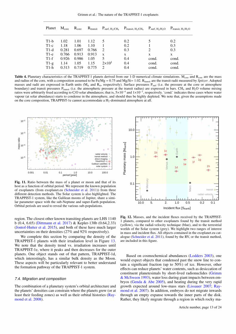
The irradiation of the TRAPPIST-1 planets plays an impor-tant role in their evolution. It is thus also insightful to comparethe TRAPPIST-1 masses and incident flux in the context of thecurrently known exoplanet population. Figure 12 shows a focuson planets receiving irradiation that spans Mars to Venus and 0.1to 4.5 M⊕. The upper mass limit is set to 4.5 M⊕ because this cor-responds to 1.5 R⊕, an indicative limit for rocky worlds (Rogers2015; Fulton et al. 2017). The lower mass limit was arbitrarilyset to 0.1 M⊕, corresponding to Mars, to represent objects thathave difficulties retaining an atmosphere. It is interesting to notethat TRAPPIST-1d & e are the only transiting exoplanets in this



Planet Mcore Rcore Rtransit Psurf, H2/CH4 Ptransit, H2/CH4 Psurf, H2/H2O Ptransit, H2/H2O

T1-b 1.02 1.01 1.12 5 0.2 5 0.2T1-c 1.18 1.06 1.10 1 0.2 1 0.3T1-d 0.281 0.697 0.766 2 0.3 2 0.3T1-e 0.766 0.913 0.913 x x x xT1-f 0.926 0.986 1.05 5 0.4 cond. cond.T1-g 1.14 1.05 1.15 2×101 0.4 cond. cond.T1-h 0.313 0.719 0.775 2 0.4 cond. cond.

Table 4. Planetary characteristics of the TRAPPIST-1 planets derived from our 1-D numerical climate simulations. Mcore and Rcore are the massand radius of the core, with a composition assumed to be Fe/Mg = 0.75 and Mg/Si= 1.02. Rtransit are the transit radii measured by Spitzer. Adoptedmasses and radii are expressed in Earth units (M⊕ and R⊕, respectively). Surface pressures Psurf (i.e. the pressure at the core or atmosphereboundary) and transit pressures Ptransit (i.e. the atmospheric pressure at the transit radius) are expressed in bars. CH4 and H2O volume mixingratios were arbitrarily fixed according to C/O solar abundances; that is, 5×10−4 and 1×10−3, respectively. ’cond.’ indicates those cases where watervapour (at solar abundance) starts to condense in the atmosphere, and should thus be highly depleted. We note that, given the assumptions madeon the core composition, TRAPPIST-1e cannot accommodate a H2-dominated atmosphere at all.

radial velocitytransit methoddirect imagingTRAPPIST−1

Galilean satellitessolar system

0.001 0.01 0.1 1.0 10.0 100.0

10−5

10−4

10−3

10−2

period [year]

mas

s ra

tio

. .

. .

Fig. 11. Ratio between the mass of a planet or moon and that of itshost as a function of orbital period. We represent the known populationof exoplanets (from exoplanet.eu (Schneider et al. 2011)) from threedifferent detection methods. The Solar system is also highlighted. TheTRAPPIST-1 system, like the Galilean moons of Jupiter, share a simi-lar parameter space with the sub-Neptune and super-Earth population.Orbital periods are used to reveal the various sub-populations.

region. The closest other known transiting planets are LHS 1140b (0.4, 6.65) (Dittmann et al. 2017) & Kepler-138b (0.64,2.33)(Jontof-Hutter et al. 2015), and both of these have much largeruncertainties on their densities (27% and 92% respectively).

We complete this section by comparing the density of theTRAPPIST-1 planets with their irradiation level in Figure 13.We note that the density trend vs. irradiation increases untilTRAPPIST-1e, where it peaks and then decreases for the outerplanets. One object stands out of that pattern, TRAPPIST-1d,which interestingly, has a similar bulk density as the Moon.These aspects will be particularly relevant to better understandthe formation pathway of the TRAPPIST-1 system.

7.4. Migration and composition

The combination of a planetary system’s orbital architecture andthe planets’ densities can constrain where the planets grew (or atleast their feeding zones) as well as their orbital histories (Ray-mond et al. 2008).

Ear

th

Ven

us

Mer

cury

Mar

s

1b1c

1d1e

1f1g

1h

transit

radial−velocity

0.11.010.0 0.22. 0.55.

0.1

1.0

10.0

. .

. . Incident flux [Searth]

Pla

neta

ry m

ass

[Mea

rth]

Fig. 12. Masses, and the incident fluxes received by the TRAPPIST-1 planets, compared to other exoplanets found by the transit method(yellow), via the radial-velocity technique (blue), and to the terrestrialworlds of the Solar system (grey). We highlight two ranges of interestin mass and incident flux. All objects contained in the exoplanet.eu cat-alogue (Schneider et al. 2011), found by the RV, or the transit method,are included in this figure.

Based on cosmochemical abundances (Lodders 2003), onewould expect objects that condensed past the snow line to con-tain a significant fraction (up to 50%) of ice. However, othereffects can reduce planets’ water contents, such as desiccation ofconstituent planetesimals by short-lived radionuclides (Grimm& McSween 1993), water loss during giant impacts between em-bryos (Genda & Abe 2005), and heating during the very rapidgrowth expected around low-mass stars (Lissauer 2007; Ray-mond et al. 2007). In addition, embryos do not migrate inwardsthrough an empty expanse towards the inner parts of the disk.Rather, they likely migrate through a region in which rocky ma-



Ear

thM

oon

Ven

us

Mer

cury

Mar

s

TRAPPIST−1

1b 1c 1d 1e 1f 1g 1h

0.11.010.0 0.22. 0.55.

4.

6.

. .

. . Incident flux [Searth]

Pla

neta

ry d

ensi

ty [g

cm

−3 ]

Fig. 13. Densities, and the incident fluxes received by the TRAPPIST-1planets (red), compared to the Solar System’s telluric planets and theMoon (grey). Other exoplanets with reported uncertainties on mass andradius smaller than 100% are shown in yellow and originate from theTEPCAT catalogue (Southworth 2011).

terial is already growing (Izidoro et al. 2014). The water contentsof migrating icy embryos are likely to be diluted by impacts withrocky embryos. In some situations, migrating icy embryos canstimulate the growth of large rocky embryos, creating a largedensity contrast between neighbouring planets (Raymond et al.2006).

Gravitational interactions with the gaseous disk cause∼Earth-mass planetary embryos to migrate, usually inwards(Ward 1997; Baruteau et al. 2014). Current models invoke twosteps in the growth of these embryos. First, as dust coagulatesand drifts through the disk (Güttler et al. 2010; Birnstiel et al.2012), 10-100 km-scale planetesimals form by a hydrodynam-ical instability (such as the streaming instability; (Youdin &Goodman 2005; Johansen et al. 2014)) in regions where the lo-cal solids-to-gas ratio is sufficiently high (Drazkowska & Dulle-mond 2014; Carrera et al. 2015). These conditions are expectedto be met first beyond the snow line (Armitage et al. 2016;Schoonenberg & Ormel 2017). Next, the largest planetesimalsgrow rapidly by accreting inwards-drifting pebbles (Ormel &Klahr 2010; Lambrechts & Johansen 2012). Models of pebbleaccretion find that large embryos preferentially grow beyond thesnow line (Morbidelli et al. 2015; Ormel et al. 2017). However,embryos’ growth is self-limiting. When an embryo reaches acritical mass, it creates a pressure bump in the gas disk exte-rior to its orbit, which traps drifting pebbles and shuts off pebbleaccretion (Lambrechts et al. 2014). This critical mass dependson the disk structure but was calculated by Ormel et al. (2017)to be ∼ 0.7M⊕ for the case of TRAPPIST-1 (for a specific diskmodel), close to the actual planet masses. In their model, em-bryos form sequentially, reaching this critical mass before mi-grating inwards.

The resonant structure of the TRAPPIST-1 system (Lugeret al. 2017) is a telltale sign of orbital migration (Terquem & Pa-paloizou 2007; Ogihara & Ida 2009). The fact that all seven plan-

ets form a single resonant chain indicates that the entire systemmigrated in concert (Cossou et al. 2014; Izidoro et al. 2017). In-deed, orbital solutions generated by disk-driven migration havebeen shown to be more stable than other solutions (Tamayo et al.2017b). Whereas most resonant systems are likely to be unstable((Izidoro et al. 2017; Matsumoto et al. 2012)), the TRAPPIST-1can be interpreted as a system that underwent a relatively slowmigration creating a long-lived resonant system.

8. Conclusions

In this paper we have used the most recent set of transit timingsof the TRAPPIST-1 system to constrain the masses, densities ofthe seven Earth-size planets found earlier this year. Our purpose-built TTV code enables an extensive exploration of the param-eter space combined to a full n-body integration scheme. Ourresults yield a significant improvement in our knowledge of theplanetary bulk density, with corresponding uncertainties rangingbetween 5 and 12%. This level of precision is unprecedented forexoplanets receiving modest irradiation in this mass range. Ourconclusions regarding the nature of the TRAPPIST-1 planets arethe following:

– The TRAPPIST-1 planets display densities ranging from 0.6to 1.0 ρ⊕.

– TRAPPIST-1 c and e likely have largely rocky interiors.– TRAPPIST-1 b, d, f, g and h require envelopes of volatiles in

the form of thick atmospheres, oceans, or ice, in most caseswith water mass fractions . 5%. For comparison, the Earth’swater content is < 0.1%.

– TRAPPIST-1 d, e, f, g and h are unlikely to have an en-riched atmosphere (e.g. CO2) above a bare core (assuminga standard Earth-like composition) without invoking unreal-istically large quantities of gas.

– TRAPPIST-1 b is the only planet above the runaway green-house limit that seems to require volatiles, with pressures ofwater vapour of the order of 101-104 bar.

These updated mass and density measurements represent keyinformation for upcoming studies straddling astrophysics, plan-etary sciences and geophysics aimed at an improved understand-ing of the interiors of temperate, Earth-sized planets.Acknowledgements. We are grateful to the referee for an helpful review that im-proved the manuscript. We thank Robert Hurt for suggesting the inclusion ofFigure 13 as well as Yann Alibert, Gavin Coleman, Apurva Oza and ChristophMordasini for insightful discussions on the TRAPPIST-1 system. B.-O.D. ac-knowledges support from the Swiss National Science Foundation (PP00P2-163967). This work has been carried out within the frame of the National Cen-tre for Competence in Research PlanetS supported by the Swiss National Sci-ence Foundation. This project has received funding from the European ResearchCouncil (ERC) under the European Union’s Horizon 2020 research and inno-vation programme (grant agreement No. 679030/WHIPLASH), and FP/2007-2013 grant agreement No. 336480, as well as from the ARC grant for ConcertedResearch Actions, financed by the Wallonia-Brussels Federation. M. Gillon,and V. Van Grootel are Belgian F.R.S.-FNRS Research Associates, E. Jehin isF.R.S.-FNRS Senior Research Associate. S.N.R. thanks the Agence Nationalepour la Recherche for support via grant ANR-13-BS05-0003-002 (grant MOJO).This work is based in part on observations made with the Spitzer Space Tele-scope, which is operated by the Jet Propulsion Laboratory, California Insti-tute of Technology under a contract with NASA. Support for this work wasprovided by NASA through an award issued by JPL/Caltech. E.A. acknowl-edges NSF grant AST-1615315, NASA grant NNX14AK26G and from theNASA Astrobiology Institute’s Virtual Planetary Laboratory Lead Team, fundedthrough the NASA Astrobiology Institute under solicitation NNH12ZDA002Cand Cooperative Agreement Number NNA13AA93A This paper includes datacollected by the K2 mission. Funding for the K2 mission is provided by theNASA Science Mission directorate. Calculations were performed on UBELIX(http://www.id.unibe.ch/hpc), the HPC cluster at the University of Bern.



ReferencesAgol, E. & Fabrycky, D. 2017, ArXiv e-prints [arXiv:1706.09849]Agol, E., Steffen, J., Sari, R., & Clarkson, W. 2005, Monthly Notices of the Royal

Astronomical Society, 359, 567Aigrain, S., Hodgkin, S. T., Irwin, M. J., Lewis, J. R., & Roberts, S. J. 2015,

Monthly Notices of the Royal Astronomical Society, 447, 2880Aigrain, S., Parviainen, H., & Pope, B. J. S. 2016, Monthly Notices of the Royal

Astronomical Society, 459, 2408Ambikasaran, S., Foreman-Mackey, D., Greengard, L., Hogg, D. W., & O’Neil,

M. 2016, IEEE T. Pattern. Anal., 38, 252Armitage, P. J., Eisner, J. A., & Simon, J. B. 2016, The Astrophysical Journall,

828, L2Asplund, M., Grevesse, N., Sauval, A. J., & Scott, P. 2009, Annual Review of

Astron and Astrophys, 47, 481Baruteau, C., Crida, A., Paardekooper, S.-J., et al. 2014, Protostars and Planets

VI, 667Birnstiel, T., Klahr, H., & Ercolano, B. 2012, Astronomy & Astrophysics, 539,

A148Bolmont, E., Raymond, S. N., Leconte, J., Hersant, F., & Correia, A. C. M. 2015,

Astronomy and Astrophysics, 583, A116Bolmont, E., Selsis, F., Owen, J. E., et al. 2017, Monthly Notices of the RAS,

464, 3728Bouchet, J., Mazevet, S., Morard, G., Guyot, F., & Musella, R. 2013, Physical

Review B, 87, 094102Braak, C. J. F. T. 2006, Statistics and Computing, 16, 239Cabrera, J., Csizmadia, S., Lehmann, H., et al. 2014, ApJ, 781, 18Canup, R. M. & Ward, W. R. 2006, Nature, 441, 834Carrera, D., Johansen, A., & Davies, M. B. 2015, Astronomy & Astrophysics,

579, A43Chambers, J. E. 1999, The Monthly Notices of the Royal Astronomical Society,

304, 793Claret, A. & Bloemen, S. 2011, Astronomy & Astrophysics, 529, A75Connolly, J. 2009, Geochemistry, Geophysics, Geosystems, 10Cossou, C., Raymond, S. N., Hersant, F., & Pierens, A. 2014, A&A, 569, A56de Wit, J., Wakeford, H. R., Gillon, M., et al. 2016, Nature, 537, 69Deck, K. M. & Agol, E. 2015, The Astrophysical Journal, 802, 116Deck, K. M., Agol, E., Holman, M. J., & Nesvorný, D. 2014, The Astrophysical

Journal, 787, 132Delrez, L., Gillon, M., Triaud, A. H. M. J., et al. 2018, Monthly Notices of the

Royal Astronomical Society, sty051Dittmann, J. A., Irwin, J. M., Charbonneau, D., et al. 2017, Nature, 544, 333Dorn, C., Venturini, J., Khan, A., et al. 2017, Astronomy & Astrophysics, 597,

A37Drazkowska, J. & Dullemond, C. P. 2014, Astronomy & Astrophysics, 572, A78Fabrycky, D. C. 2010, ArXiv e-prints [arXiv:1006.3834]Foreman-Mackey, D., Hogg, D. W., Lang, D., & Goodman, J. 2013, Publications

of the Astronomical Society of the Pacific, 125, 306Fulton, B. J., Petigura, E. A., Howard, A. W., et al. 2017, AJ, 154, 109Genda, H. & Abe, Y. 2005, Nature, 433, 842Gillon, M., Demory, B.-O., Benneke, B., et al. 2012, Astronomy & Astrophysics,

539, A28Gillon, M., Jehin, E., Lederer, S. M., et al. 2016, Nature, 533, 221Gillon, M., Triaud, A. H. M. J., Demory, B.-O., et al. 2017, Nature, 542, 456Gimenez, A. & Garcia-Pelayo, J. M. 1983, Ap&SS, 92, 203Goodman, J. & Weare, J. 2010, Communications in Applied Mathematics and

Computational Science, Vol. 5, No. 1, p. 65-80, 2010, 5, 65Gozdziewski, K., Migaszewski, C., Panichi, F., & Szuszkiewicz, E. 2016, The

Monthly Notices of the Royal Astronomical Society, 455, L104Grimm, R. E. & McSween, H. Y. 1993, Science, 259, 653Grimm, S. L. & Stadel, J. G. 2014, The Astrophysical Journal, 796, 23Güttler, C., Blum, J., Zsom, A., Ormel, C. W., & Dullemond, C. P. 2010, Astron-

omy & Astrophysics, 513, A56Hernandez, D. M. & Bertschinger, E. 2015, Monthly Notices of the Royal As-

tronomical Society, 452, 1934Holman, M. J. 2005, Science, 307, 1288Holman, M. J., Fabrycky, D. C., Ragozzine, D., et al. 2010, Science, 330, 51Howard, A. W., Marcy, G. W., Bryson, S. T., et al. 2012, The Astrophysical

Journal Supp., 201, 15Howell, S. B., Sobeck, C., Haas, M., et al. 2014, Publications of the Astronomical

Society of the Pacific, 126, 398Izidoro, A., Morbidelli, A., & Raymond, S. N. 2014, The Astrophysical Journal,

794, 11Izidoro, A., Ogihara, M., Raymond, S. N., et al. 2017, MNRAS, 470, 1750Johansen, A., Blum, J., Tanaka, H., et al. 2014, Protostars and Planets VI, 547Jontof-Hutter, D., Lissauer, J. J., Rowe, J. F., & Fabrycky, D. C. 2014, The As-

trophysical Journal, 785, 15Jontof-Hutter, D., Rowe, J. F., Lissauer, J. J., Fabrycky, D. C., & Ford, E. B.

2015, Nature, 522, 321

Kopparapu, R. K., Ramirez, R., Kasting, J. F., et al. 2013, Astrophysical Journal,765, 131

Kopparapu, R. k., Wolf, E. T., Haqq-Misra, J., et al. 2016, Astrophysical Journal,819, 84

Lambrechts, M. & Johansen, A. 2012, Astronomy & Astrophysics, 544, A32Lambrechts, M., Johansen, A., & Morbidelli, A. 2014, Astronomy & Astro-

physics, 572, A35Lissauer, J. J. 2007, The Astrophysical Journal Letters, 660, L149Lithwick, Y., Xie, J., & Wu, Y. 2012, The Astrophysical Journal, 761, 122Lodders, K. 2003, The Astrophysical Journal, 591, 1220Luger, R., Sestovic, M., Kruse, E., et al. 2017, Nature Astronomy, 1, 0129Mandel, K. & Agol, E. 2002, The Astrophysical Journal Letters, 580, L171Matsumoto, Y., Nagasawa, M., & Ida, S. 2012, Icarus, 221, 624Mayor, M., Marmier, M., Lovis, C., et al. 2011, ArXiv e-printsMills, S. M., Fabrycky, D. C., Migaszewski, C., et al. 2016, Nature, 533, 509Morbidelli, A., Lambrechts, M., Jacobson, S., & Bitsch, B. 2015, Icarus, 258,

418Neron de Surgy, O. & Laskar, J. 1997, Astronomy and Astrophysics, 318, 975Nesvorný, D. & Vokrouhlický, D. 2014, ApJ, 790, 58Ogihara, M. & Ida, S. 2009, The Astrophysical Journal, 699, 824Ormel, C. W. & Klahr, H. H. 2010, Astronomy & Astrophysics, 520, A43Ormel, C. W., Liu, B., & Schoonenberg, D. 2017, A&A, 604, A1Quarles, B., Quintana, E. V., Lopez, E., Schlieder, J. E., & Barclay, T. 2017, The

Astrophysical Journal Letters, 842, L5Raymond, S. N., Barnes, R., & Mandell, A. M. 2008, The Monthly Notices of

the Royal Astronomical Society, 384, 663Raymond, S. N., Mandell, A. M., & Sigurdsson, S. 2006, Science, 313, 1413Raymond, S. N., Scalo, J., & Meadows, V. S. 2007, The Astrophysical Journal,

669, 606Rogers, L. A. 2015, ApJ, 801, 41Schneider, J., Dedieu, C., Le Sidaner, P., Savalle, R., & Zolotukhin, I. 2011,

Astronomy and Astrophysics, 532, A79Schoonenberg, D. & Ormel, C. W. 2017, Astronomy & Astrophysics, 602, A21Seager, S., Kuchner, M., Hier-Majumder, C., & Militzer, B. 2007, The Astro-

physical Journal, 669, 1279Seager, S. & Mallén-Ornelas, G. 2003, The Astrophysical Journal, 585, 1038Southworth, J. 2011, MNRAS, 417, 2166Spencer, J. R., Rathbun, J. A., Travis, L. D., et al. 2000, Science, 288, 1198Storn, R. & Price, K. 1997, J. Global Optim., 11, 341Tamayo, D., Rein, H., Petrovich, C., & Murray, N. 2017a, The Astrophysical

Journall, 840, L19Tamayo, D., Rein, H., Petrovich, C., & Murray, N. 2017b, The Astrophysical

Journal Letters, 840, L19Terquem, C. & Papaloizou, J. C. B. 2007, The Astrophysical Journal, 654, 1110Turbet, M., Bolmont, E., Leconte, J., et al. 2017, ArXiv e-prints

[arXiv:1707.06927]Unterborn, C. T., Desch, S. J., Hinkel, N., & Lorenzo, A. 2017, ArXiv e-printsVan Grootel, V., Fernandes, C. S., Gillon, M., et al. 2018, ApJ, 853, 30Vazan, A., Kovetz, A., Podolak, M., & Helled, R. 2013, Monthly Notices of the

Royal Astronomical Society, 434, 3283Vrugt, J. A., Ter Braak, C., Diks, C., et al. 2009, International Journal of Nonlin-

ear Sciences and Numerical Simulation, 10, 273Waldmann, I. P., Tinetti, G., Rocchetto, M., et al. 2015, Astrophysical Journal,

802, 107Wang, S., Wu, D.-H., Barclay, T., & Laughlin, G. P. 2017, ArXiv e-printsWard, W. R. 1997, Icarus, 126, 261Wisdom, J. & Hernandez, D. M. 2015, Monthly Notices of the Royal Astronom-

ical Society, 453, 3015Wordsworth, R. D., Forget, F., Selsis, F., et al. 2010, Astronomy and Astro-

physics, 522, A22Youdin, A. N. & Goodman, J. 2005, The Astrophysical Journal, 620, 459



Appendix A: Transit timings



Mid-transit time [BJDTDB] uncertainty [days] Source2457322.51531 0.00071 TS (Gillon et al. 2016)2457325.53910 0.00100 TS (Gillon et al. 2016)2457328.55860 0.00130 TS2457331.58160 0.00100 TS (Gillon et al. 2016)2457334.60480 0.00017 VLT (Gillon et al. 2016)2457337.62644 0.00092 TS (Gillon et al. 2016)2457340.64820 0.00140 TS (Gillon et al. 2016)2457345.18028 0.00080 HCT (Gillon et al. 2016)2457361.79945 0.00028 UK (Gillon et al. 2016)2457364.82173 0.00077 UK (Gillon et al. 2016)2457440.36492 0.00020 Sp (Gillon et al. 2017)2457452.45228 0.00014 Sp (Gillon et al. 2017)2457463.02847 0.00019 Sp (Gillon et al. 2017)2457509.86460 0.00210 TS (Gillon et al. 2017)2457512.88731 0.00029 HST (de Wit et al. 2016)2457568.78880 0.00100 TS (Gillon et al. 2017)2457586.91824 0.00064 TS (Gillon et al. 2017)2457589.93922 0.00092 TS (Gillon et al. 2017)2457599.00640 0.00021 UK (Gillon et al. 2017)2457602.02805 0.00071 UK (Gillon et al. 2017)2457612.60595 0.00085 TN (Gillon et al. 2017)2457615.62710 0.00160 TS (Gillon et al. 2017)2457624.69094 0.00066 TN (Gillon et al. 2017)2457645.84400 0.00110 WHT (Gillon et al. 2017)2457651.88743 0.00022 Sp (Gillon et al. 2017)2457653.39809 0.00026 Sp (Gillon et al. 2017)2457654.90908 0.00084 Sp (Gillon et al. 2017)2457656.41900 0.00029 TN+LT (Gillon et al. 2017)2457657.93129 0.00020 Sp (Gillon et al. 2017)2457659.44144 0.00017 Sp (Gillon et al. 2017)2457660.95205 0.00035 Sp (Gillon et al. 2017)2457662.46358 0.00020 Sp (Gillon et al. 2017)

Table A.1. Planet b. TS/TN stands for TRAPPIST-South/-North, VLT for the Very Large Telescope with the HAWK-I instrument, HCT for theHimalayan Chandra Telescope, UK for UKIRT, Sp for Spitzer with the IRAC instrument, HST for the Hubble Space Telescope with the WFC3instrument, WHT for the William Herschel Telescope, LT for the Liverpool Telescope, SSO for the Speculoos Southern Observatory.



Mid-transit time [BJDTDB] uncertainty [days] Source2457663.97492 0.00070 Sp (Gillon et al. 2017)2457665.48509 0.00017 Sp (Gillon et al. 2017)2457666.99567 0.00025 Sp (Gillon et al. 2017)2457668.50668 0.00030 Sp (Gillon et al. 2017)2457670.01766 0.00034 Sp (Gillon et al. 2017)2457671.52876 0.00033 Sp (Gillon et al. 2017)2457721.38747 0.00035 TN2457739.51770 0.00059 K22457741.02787 0.00055 K22457742.53918 0.00058 K22457744.05089 0.00061 K22457745.56164 0.00072 K22457747.07208 0.00085 K22457748.58446 0.00087 K22457750.09387 0.00089 K22457751.60535 0.00082 K22457753.11623 0.00075 K22457754.62804 0.00077 K22457756.13856 0.00060 K22457757.64840 0.00089 K22457759.15953 0.00073 K22457760.67112 0.00082 K22457762.18120 0.00073 K22457763.69221 0.00071 K22457765.20298 0.00077 K22457766.71479 0.00055 K22457768.22514 0.00103 K22457769.73704 0.00064 K22457771.24778 0.00091 K22457772.75738 0.00075 K22457774.26841 0.00080 K22457775.77995 0.00058 K22457777.28899 0.00099 K22457778.80118 0.00062 K22457780.31297 0.00068 K22457781.82231 0.00145 K22457783.33410 0.00071 K22457784.84372 0.00068 K22457792.39979 0.00110 K22457793.90955 0.00064 K2

Table A.2. Continued.



Mid-transit time [BJDTDB] uncertainty [days] Source2457795.41987 0.00058 K22457796.93134 0.00065 K22457798.44211 0.00061 K22457799.95320 0.00083 K22457801.46314 0.00127 K22457802.97557 0.00016 Sp + K22457804.48638 0.00053 K22457805.99697 0.00016 Sp + K22457807.50731 0.00017 Sp + K22457809.01822 0.00017 Sp + K22457810.52781 0.00110 K22457812.04038 0.00020 Sp + K22457813.55121 0.00014 Sp + K22457815.06275 0.00017 Sp + K22457816.57335 0.00011 Sp + K22457818.08382 0.00015 Sp2457819.59478 0.00017 Sp2457821.10550 0.00020 Sp2457824.12730 0.00018 Sp2457825.63813 0.00018 Sp2457827.14995 0.00012 Sp2457828.66042 0.00024 Sp2457830.17087 0.00021 Sp2457833.19257 0.00018 Sp2457834.70398 0.00016 Sp2457836.21440 0.00017 Sp2457837.72526 0.00014 Sp2457839.23669 0.00017 Sp2457917.80060 0.00110 TS2457923.84629 0.00045 SSO2457935.93288 0.00023 SSO2457952.55450 0.00110 TN2457955.57554 0.00069 TN2457967.66254 0.00050 SSO2457973.70596 0.00040 SSO




Mid-transit time [BJDTDB] uncertainty [days] Source2457282.80570 0.00140 TS (Gillon et al. 2016)2457333.66400 0.00090 TS (Gillon et al. 2016)2457362.72605 0.00038 UK (Gillon et al. 2016)2457367.57051 0.00033 TS+VLT (Gillon et al. 2016, 2017)2457384.52320 0.00130 TS (Gillon et al. 2016)2457452.33470 0.00015 Sp (Gillon et al. 2017)2457454.75672 0.00066 Sp (Gillon et al. 2017)2457512.88094 0.00009 HST (de Wit et al. 2016)2457546.78587 0.00075 TS (Gillon et al. 2017)2457551.62888 0.00066 TS (Gillon et al. 2017)2457580.69137 0.00031 LT (Gillon et al. 2017)2457585.53577 0.00250 TN (Gillon et al. 2017)2457587.95622 0.00054 TS+UK (Gillon et al. 2017)2457600.06684 0.00036 UK (Gillon et al. 2017)2457604.90975 0.00063 TS (Gillon et al. 2017)2457609.75461 0.00072 TS (Gillon et al. 2017)2457614.59710 0.00130 TS (Gillon et al. 2017)2457626.70610 0.00110 TS (Gillon et al. 2017)2457631.55024 0.00056 TN+TS (Gillon et al. 2017)2457638.81518 0.00048 TS (Gillon et al. 2017)2457650.92395 0.00023 Sp (Gillon et al. 2017)2457653.34553 0.00024 Sp (Gillon et al. 2017)2457655.76785 0.00043 Sp (Gillon et al. 2017)2457658.18963 0.00024 Sp (Gillon et al. 2017)2457660.61168 0.00051 Sp (Gillon et al. 2017)2457663.03292 0.00028 Sp (Gillon et al. 2017)2457665.45519 0.00025 Sp (Gillon et al. 2017)2457667.87729 0.00031 Sp (Gillon et al. 2017)2457670.29869 0.00035 Sp (Gillon et al. 2017)2457672.71944 0.00081 Sp (Gillon et al. 2017)2457711.46778 0.00064 TN2457723.57663 0.00050 TS2457740.53361 0.00088 K22457742.95276 0.00115 K22457745.37429 0.00063 K2

Table A.4. Planet c



Mid-transit time [BJDTDB] uncertainty [days] Source2457747.79699 0.00056 K22457750.21773 0.00096 K22457752.64166 0.00093 K22457755.05877 0.00165 K22457757.48313 0.00066 K22457759.90281 0.00058 K22457762.32806 0.00081 K22457764.74831 0.00072 K22457767.16994 0.00125 K22457769.59209 0.00081 K22457772.01483 0.00100 K22457774.43458 0.00081 K22457776.85815 0.00102 K22457779.27911 0.00089 K22457781.70095 0.00072 K22457784.12338 0.00054 K22457791.38801 0.00064 K22457793.81141 0.00079 K22457796.23153 0.00052 K22457798.65366 0.00082 K22457801.07631 0.00084 K22457803.49747 0.00020 Sp + K22457805.91882 0.00017 Sp + K22457808.34123 0.00023 Sp + K22457810.76273 0.00019 Sp + K22457813.18456 0.00024 Sp + K22457815.60583 0.00017 Sp + K22457818.02821 0.00020 Sp2457820.45019 0.00022 Sp2457822.87188 0.00021 Sp2457825.29388 0.00022 Sp2457827.71513 0.00022 Sp2457830.13713 0.00026 Sp2457832.55888 0.00015 Sp2457834.98120 0.00025 Sp2457837.40280 0.00017 Sp2457839.82415 0.00031 Sp




Mid-transit time [BJDTDB] uncertainty [days] Source2457560.79730 0.00230 TS (Gillon et al. 2017)2457625.59779 0.00078 WHT (Gillon et al. 2017)2457641.79360 0.00290 TS (Gillon et al. 2017)2457645.84360 0.00210 TS (Gillon et al. 2017)2457653.94261 0.00051 Sp (Gillon et al. 2017)2457657.99220 0.00063 Sp (Gillon et al. 2017)2457662.04284 0.00051 Sp (Gillon et al. 2017)2457666.09140 0.00160 Sp (Gillon et al. 2017)2457670.14198 0.00066 Sp (Gillon et al. 2017)2457726.83975 0.00029 HST2457738.99169 0.00160 K22457743.03953 0.00180 K22457747.08985 0.00145 K22457751.14022 0.00195 K22457755.18894 0.00155 K22457759.24638 0.00225 K22457763.28895 0.00150 K22457767.33866 0.00190 K22457771.39077 0.00260 K22457775.44026 0.00125 K22457779.48843 0.00190 K22457783.54023 0.00240 K22457791.64083 0.00135 K22457803.79083 0.00049 Sp + K22457807.84032 0.00030 Sp + K22457811.89116 0.00050 Sp + K22457815.94064 0.00030 Sp + K22457819.99050 0.00050 Sp2457824.04185 0.00067 Sp2457828.09082 0.00043 Sp2457832.14036 0.00037 Sp2457836.19171 0.00042 Sp2457961.73760 0.00130 SSO+TS2457969.83708 0.00068 SSO2457973.88590 0.00066 SSO

Table A.6. Planet d



Mid-transit time [BJDTDB] uncertainty [days] Source2457312.71300 0.00270 TS (Gillon et al. 2017)2457367.59683 0.00037 TS+VLT (Gillon et al. 2016, 2017)2457611.57620 0.00310 TN (Gillon et al. 2017)2457623.77950 0.00100 TS (Gillon et al. 2017)2457654.27862 0.00049 Sp (Gillon et al. 2017)2457660.38016 0.00078 Sp (Gillon et al. 2017)2457666.48030 0.00180 TS+LT (Gillon et al. 2017)2457672.57930 0.00260 TS (Gillon et al. 2017)2457721.37514 0.00099 TN (Gillon et al. 2017)2457733.57300 0.00140 TS2457739.67085 0.00135 K22457745.77160 0.00120 K22457751.87007 0.00034 HST2457757.96712 0.00160 K22457764.06700 0.00240 K22457770.17109 0.00215 K22457776.26378 0.00160 K22457782.36226 0.00175 K22457794.56159 0.00160 K22457800.66354 0.00170 K22457806.75758 0.00041 Sp + K22457812.85701 0.00034 Sp + K22457818.95510 0.00030 Sp2457825.05308 0.00035 Sp2457831.15206 0.00027 Sp2457837.24980 0.00025 Sp2457934.83095 0.00050 SSO+TS2457940.92995 0.00086 SSO

Table A.7. Planet e

Mid-transit time [BJDTDB] uncertainty [days] Source2457321.52520 0.00200 TS (Gillon et al. 2017)2457367.57629 0.00044 TS+VLT (Gillon et al. 2016, 2017)2457634.57809 0.00061 TS+LT (Gillon et al. 2017)2457652.98579 0.00032 Sp (Gillon et al. 2017)2457662.18747 0.00040 Sp (Gillon et al. 2017)2457671.39279 0.00072 Sp (Gillon et al. 2017)2457717.41541 0.00091 TN (Gillon et al. 2017)2457726.61960 0.00026 TS (Gillon et al. 2017)2457745.03116 0.00135 K22457754.23380 0.00155 K22457763.44338 0.00024 HST2457772.64752 0.00160 K22457781.85142 0.00180 K22457800.27307 0.00140 K22457809.47554 0.00027 Sp + K22457818.68271 0.00032 Sp2457827.88669 0.00030 Sp2457837.10322 0.00032 Sp2457956.80549 0.00054 SSO+HST

Table A.8. Planet f



Mid-transit time [BJDTDB] uncertainty [days] Source2457294.78600 0.00390 TS (Gillon et al. 2016)2457356.53410 0.00200 TS (Gillon et al. 2017)2457615.92400 0.00170 TS (Gillon et al. 2017)2457640.63730 0.00100 TS (Gillon et al. 2017)2457652.99481 0.00030 Sp (Gillon et al. 2017)2457665.35151 0.00028 Sp (Gillon et al. 2017)2457739.48441 0.00115 K22457751.83993 0.00017 HST2457764.19098 0.00155 K22457776.54900 0.00110 K22457801.25000 0.00093 K22457813.60684 0.00023 Sp + K22457825.96112 0.00020 Sp2457838.30655 0.00028 Sp2457924.77090 0.00140 SSO+TS2457961.82621 0.00068 SSO+TS

Table A.9. Planet g

Mid-transit time [BJDTDB] uncertainty [days] Source2457662.55467 0.00054 Sp (Gillon et al. 2017; Luger et al. 2017)2457756.38740 0.00130 K22457775.15390 0.00160 K22457793.92300 0.00250 K22457812.69870 0.00450 K22457831.46625 0.00047 Sp2457962.86271 0.00083 SSO

Table A.10. Planet h


the nature of the trappist-1 exoplanets

Documents