The National Dam Safety ProgramFinal Report on Coordination and Cooperation with theEuropean Union on Embankment Failure Analysis

FEMA 602 / August 2007

REPORT This report is submitted as the final report by Dr. Greg Hanson and Darrel Temple of the USDA-ARS-HERU. PROJECT SPONSOR Federal Emergency Management Agency National Dam Safety Program Research Subcommittee 500 C Street SW Washington, DC 20047 PROJECT COORDINATOR Dr. Greg Hanson USDA-ARS-HERU 1301 N. Western Stillwater, OK 74075 REFERENCE CONTRACT NO. EMW-2003-IA-0256, M003

Contents List 1.0 Introduction…………………………………………………………………………… 4

1.1 Overview………………………………………………………………………. …. 4 1.2 Background…………………………………………………………………….…. 4

2.0 Research Activities of Erosion Mechanics of Overtopped Embankments…........ 6

2.1 Review…………………………………………………………………………….... 6 2.2 Description of Field and Laboratory Research Tests……………………….…. 7

2.2.1 Small-scale Laboratory Tests of Breach Formation – UK…………………. 7 2.2.1.1 Series #1 – 0.5 m Small Scale Embankment Overtopping Tests….. 7 2.2.1.2 Series #2 – 0.6 m Small Scale Embankment Overtopping Tests….. 7 2.2.1.3 Series #3 – Small Scale Internal Erosion Tests……………...………. 7

2.2.2 Large-scale Field Tests of Breach Formation – Norway…………..……… 7 2.2.3 Embankment Overtopping Research – US………………………..……….. 9

2.2.3.1 Steep Grass and Bare Earth Channel Tests………………..…….... 10 2.2.3.2 Large-scale Flume Studies of Headcut Migration…………………....10 2.2.3.3 Large-scale Tests of Breach Initiation and Formation…….….…..... 11 2.2.3.3 Large-scale Tests of Breach Widening……………………..……….. 12

2.3 Summary of Results Related to Cohesive Embankment Tests…….………. 13 2.4 Lessons Learned from Cohesive Embankment Breach Tests….…………… 13

2.4.1 Observed Erosion Processes of Cohesive Embankments…………..….. 13 2.4.2 Initiation and Formation Time……………………….……………………… 16 2.4.3 Rate of Erosion and Compaction Effects…….......................................... 17

3.0 Workshop ……………………………………………………………………………. 18

3.1 Summary of Workshop Papers………………………………………………… 18 3.1.1 Paper 1 ………………………………………………………………………. 18 3.1.2 Paper 2 ………………………………………………………………………. 19 3.1.3 Paper 3 ………………………………………………………………………. 19 3.1.4 Paper 4 ………………………………………………………………………. 19 3.1.5 Paper 5 ………………………………………………………………………. 19 3.1.6 Paper 6 ………………………………………………………………………. 20 3.1.7 Paper 7 ………………………………………………………………………. 20 3.1.8 Paper 8 ………………………………………………………………………. 20 3.1.9 Paper 9 ………………………………………………………………………. 21 3.1.10 Paper 10 ……………………………………………………………………….21

4.0 Conclusions…………………………………………………………………………….21 5.0 References……………………………………………………………………………. 22 6.0 Appendix (Workshop Papers 1 – 10)………………………………………………. 24

1. INTRODUCTION 1.1 Overview The US Dam Safety community has similar needs and activities to those of the European (EU) Dam Safety community. There has been an emphasis in the EU community on investigation of extreme flood processes and the uncertainties related to these processes. The purpose of this project was to cooperate with the organizations involved in these investigations over a three year period. The purpose of this cooperation was to: 1) coordinate US and EU efforts and collect information necessary to integrate data and knowledge with US activities and interests related to embankment overtopping and failure analysis, 2) Utilize the data obtained by both groups to improve embankment failure analysis methods, and 3) provide dissemination of these activities and their results to the US dam safety community. Dissemination was to be accomplished by:

1) Conducting a special workshop at a professional society meeting involving invited speakers from Europe and the United States. This session was held as a one day workshop at the Annual Conference of the Association of State Dam Safety Officials 2004 Dam Safety. The title of the day long workshop was; “Workshop on International Progress in Dam Breach Evaluation.” Ten presentations were included in the workshop (see appendix for manuscripts).

2) A final report integrating EU and US research findings and results related to

earthen embankment overtopping failure over the 3-year period would be developing and reporting in the form of a FEMA/USDA document. This report is included in the following pages.

1.2 Background Sending U.S. representatives to cooperate with EU was included in the research needs identified by participants in the FEMA, “Workshop on Issues, Resolutions, and Research Needs Related to Embankment Dam Failure Analysis,” held June 26-28th, 2001, in Oklahoma City, OK. The prioritized list of fourteen research needs, taken from the proceedings of this workshop (USDA, 2001), is shown in table 1. This list was based on an aggregate score of votes by the workshop participants on value, cost, and probability of success of the specified research needs. Topic number 13 (No. 7 priority ranking) of the research list, cooperation with EU dam failure analysis activities, contributes to addressing topic numbers 4, 5, 7, 10, 11, and 12, with priority rankings of 10, 3, 5, 13, 11, and 2 respectively. Both the US and EU have had research activities related to prediction of performance of earth embankment dams during extreme flood events. These projects including; the EU Concerted Action on Dambreak Modeling (CADAM) project, Investigation of Extreme Flood Processes and Uncertainty (IMPACT), Integrated Flood Risk Analysis and Management Methodologies (FLOODsite) (Morris et al., 2004), and the work of USDA-

4

Agricultural Research Service to address overtopping of aging dams were summarized in the workshop proceedings (USDA, 2001). These projects are seen to have a number of complimentary concerns and goals. Within these projects there has been a component of research focused on erosion mechanics of overtopped earthen embankments including physical and numerical modeling. This report focuses on the effort of both groups in this area and on integrating these findings. TABLE 1 – RESEARCH TOPICS RANKED BY AGGREGATE SCORE TOPIC NUMBER RESEARCH / DEVELOPMENT TOPIC(S) AGGREGATE

SCORE RANK

2

Develop forensic guidelines and standards for dam safety experts to use when reporting dam failures or dam incidents. Create a forensic team that would be able to collect and disseminate valuable forensic data.

54 1

12 Using physical research data, develop guidance for the selection of breach parameters used during breach modeling. 52 2

5

Perform basic physical research to model different dam parameters such as soil properties, scaling effects, etc. with the intent to verify the ability to model actual dam failure characteristics and extend dam failure knowledge using scale models.

40 3

1 Update, Revise, and Disseminate the historic data set / database. The data set should include failure information, flood information, and embankment properties.

38 4

7 Develop better computer-based predictive models. Preferably build upon existing technology rather than developing new software. 34 5

9

Make available hands-on end-user training for breach and flood routing modeling that is available to government agencies and regulators, public entities (such as dam owners), and private consultants.

30 6

13 Send U.S. representatives to cooperate with EU dam failure analysis activities. 30 7

3 Record an expert-level video of Danny Fread along the lines of the ICODS videos from Jim Mitchell, Don Deer, etc. 29 8

6 Update the regression equations used to develop the input data used in dam breach and flood routing models. 20 9

4 Identify critical parameters for different types of failure modes 14 10

11 Develop a method to combine deterministic and probabilistic dam failure analyses including the probability of occurrence and probable breach location.

10 11

14 Lobby the NSF to fund basic dam failure research. 4 12

10 Validate and test existing dam breach and flood routing models using available dam failure information. 2 13

8 Develop a process that would be able to integrate dam breach and flood routing information into an early warning system. 0 14

5

2.0 RESEARCH ON EROSION MECHANICS OF OVERTOPPED EMBANKMENT

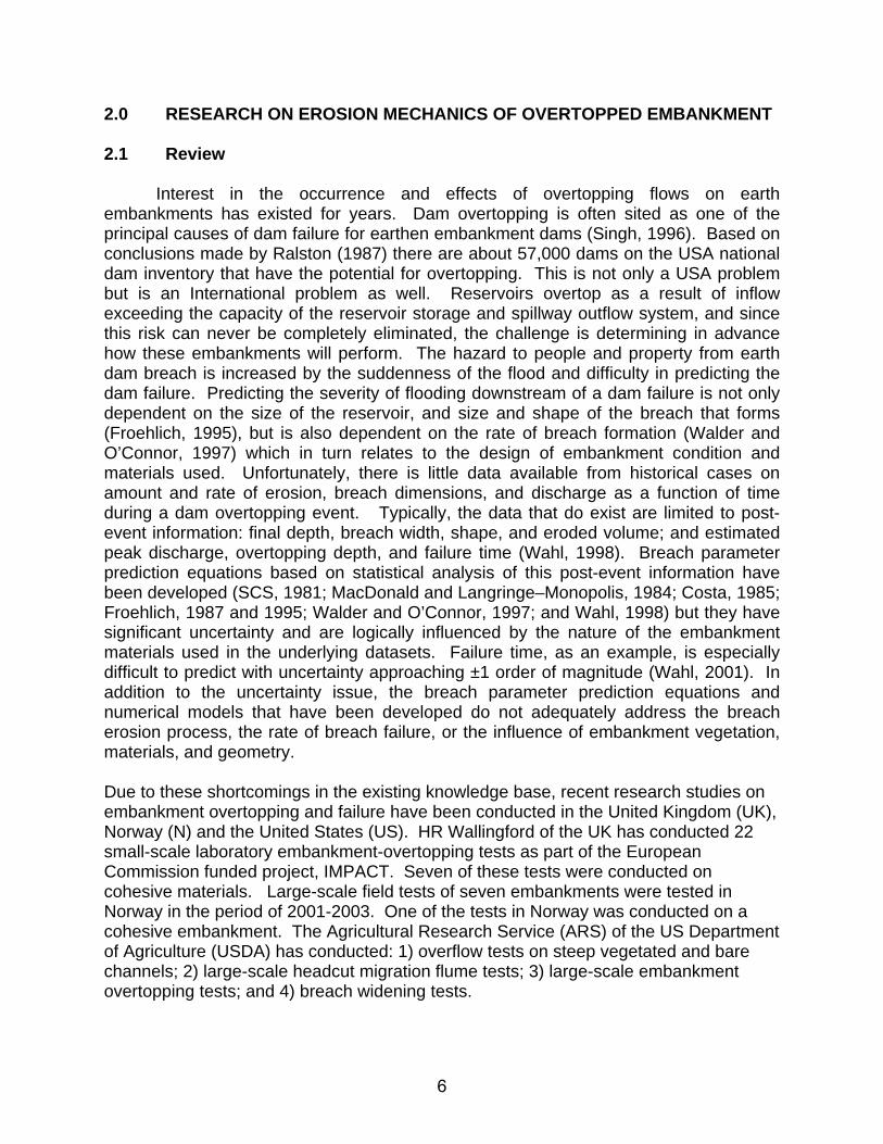
2.1 Review

Interest in the occurrence and effects of overtopping flows on earth embankments has existed for years. Dam overtopping is often sited as one of the principal causes of dam failure for earthen embankment dams (Singh, 1996). Based on conclusions made by Ralston (1987) there are about 57,000 dams on the USA national dam inventory that have the potential for overtopping. This is not only a USA problem but is an International problem as well. Reservoirs overtop as a result of inflow exceeding the capacity of the reservoir storage and spillway outflow system, and since this risk can never be completely eliminated, the challenge is determining in advance how these embankments will perform. The hazard to people and property from earth dam breach is increased by the suddenness of the flood and difficulty in predicting the dam failure. Predicting the severity of flooding downstream of a dam failure is not only dependent on the size of the reservoir, and size and shape of the breach that forms (Froehlich, 1995), but is also dependent on the rate of breach formation (Walder and O’Connor, 1997) which in turn relates to the design of embankment condition and materials used. Unfortunately, there is little data available from historical cases on amount and rate of erosion, breach dimensions, and discharge as a function of time during a dam overtopping event. Typically, the data that do exist are limited to post-event information: final depth, breach width, shape, and eroded volume; and estimated peak discharge, overtopping depth, and failure time (Wahl, 1998). Breach parameter prediction equations based on statistical analysis of this post-event information have been developed (SCS, 1981; MacDonald and Langringe–Monopolis, 1984; Costa, 1985; Froehlich, 1987 and 1995; Walder and O’Connor, 1997; and Wahl, 1998) but they have significant uncertainty and are logically influenced by the nature of the embankment materials used in the underlying datasets. Failure time, as an example, is especially difficult to predict with uncertainty approaching ±1 order of magnitude (Wahl, 2001). In addition to the uncertainty issue, the breach parameter prediction equations and numerical models that have been developed do not adequately address the breach erosion process, the rate of breach failure, or the influence of embankment vegetation, materials, and geometry. Due to these shortcomings in the existing knowledge base, recent research studies on embankment overtopping and failure have been conducted in the United Kingdom (UK), Norway (N) and the United States (US). HR Wallingford of the UK has conducted 22 small-scale laboratory embankment-overtopping tests as part of the European Commission funded project, IMPACT. Seven of these tests were conducted on cohesive materials. Large-scale field tests of seven embankments were tested in Norway in the period of 2001-2003. One of the tests in Norway was conducted on a cohesive embankment. The Agricultural Research Service (ARS) of the US Department of Agriculture (USDA) has conducted: 1) overflow tests on steep vegetated and bare channels; 2) large-scale headcut migration flume tests; 3) large-scale embankment overtopping tests; and 4) breach widening tests.

6

This report provides a summary of research activity focusing on overtopped cohesive earth embankment tests in the UK, Norway, and the US. It is hoped that the data from these research activities can: 1) establish a better understanding of the embankment breaching processes; 2) determine the rate of breach of cohesive embankments; 3) provide data for numerical model validation, calibration and testing, and hence improve modeling tool performance; and 4) provide information and data to assess the scaling effect between field and laboratory experiments. 2.2 Description of Field and Laboratory Research Tests

The entities conducting the embankment breach research described herein each have unique facilities, expertise, and perspective on the problems to be addressed. The studies conducted are briefly described below. 2.2.1 Small-scale laboratory tests of breach formation – UK A total of 22 laboratory experiments were undertaken at HR Wallingford in the UK (Hassan et al., 2004). The overall objective of these tests was to better understand the breach processes in embankments failed by overtopping or internal erosion and identify the important parameters that influence these processes: 2.2.1.4 Series #1 – 0.5 m Small scale embankment overtopping tests.

Nine tests were conducted on homogeneous non-cohesive 0.5-m high by 6-m long embankments. Each embankment was constructed from non-cohesive material, with more than one grading of sand used along with different embankment geometries, breach locations, and seepage rates. The three gradings used in testing were: 1) uniform coarse grading with a D50 of 0.70-0.90 mm; 2) uniform fine grading with D50 = 0.25 mm; and 3) wide grading with a D50=0.25 mm.

2.2.1.5 Series #2 – 0.6 m Small scale embankment overtopping tests.

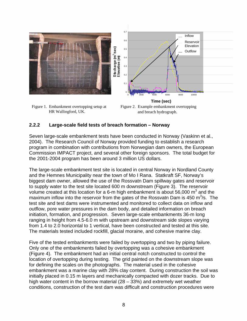
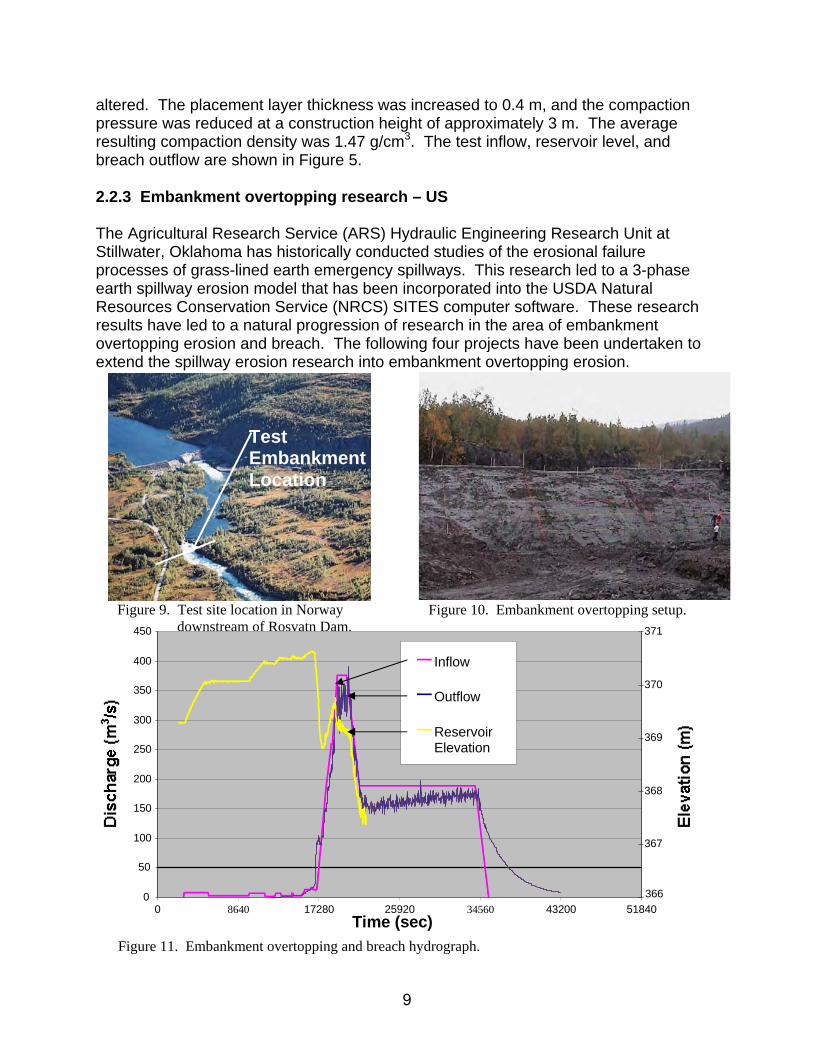
Eight tests were conducted on homogeneous cohesive 0.6-m high by 4-m long embankments (Figure 1). Seven embankments were constructed from a cohesive soil material having a D50 = 0.005 mm with 43% clay and one embankment was built from a moraine material with D50 = 0.715 mm with 10% fines. The seven cohesive embankments were constructed using two different compaction efforts and various water contents. One compaction effort was half the other based on the number of drops of a hand-tamping tool. The compaction water content ranged from 19 to 28% for the seven tests. The resulting compaction densities ranged from 1.13 to 1.23 g/cm3. The physical modeling set-up and results including; inflow, outflow, and reservoir water surface elevations for one of the cohesive embankment overtopping breach tests are shown in Figures 1 and 2.

2.2.1.6 Series #3 – Small scale internal erosion tests.

Five tests on homogeneous moraine and actual river embankment materials were conducted to assess mechanisms and dimensions associated with the initiation of internal erosion.

7

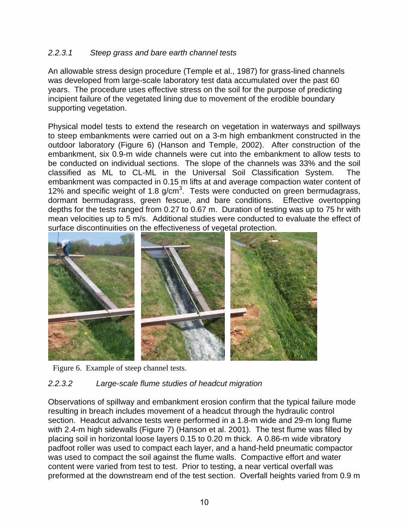
2.2.2 Large-scale field tests of breach formation – Norway Seven large-scale embankment tests have been conducted in Norway (Vaskinn et al., 2004). The Research Council of Norway provided funding to establish a research program in combination with contributions from Norwegian dam owners, the European Commission IMPACT project, and several other foreign sponsors. The total budget for the 2001-2004 program has been around 3 million US dollars. The large-scale embankment test site is located in central Norway in Nordland County and the Hemnes Municipality near the town of Mo I Rana. Statkraft SF, Norway’s biggest dam owner, allowed the use of the Rossvatn Dam spillway gates and reservoir to supply water to the test site located 600 m downstream (Figure 3). The reservoir volume created at this location for a 6-m high embankment is about 56,000 m3 and the maximum inflow into the reservoir from the gates of the Rossvatn Dam is 450 m3/s. The test site and test dams were instrumented and monitored to collect data on inflow and outflow, pore water pressures in the dam body, and detailed information on breach initiation, formation, and progression. Seven large-scale embankments 36-m long ranging in height from 4.5-6.0 m with upstream and downstream side slopes varying from 1.4 to 2.0 horizontal to 1 vertical, have been constructed and tested at this site. The materials tested included rockfill, glacial moraine, and cohesive marine clay. Five of the tested embankments were failed by overtopping and two by piping failure. Only one of the embankments failed by overtopping was a cohesive embankment (Figure 4). The embankment had an initial central notch constructed to control the location of overtopping during testing. The grid painted on the downstream slope was for defining the scales on the photographs. The material used in the cohesive embankment was a marine clay with 28% clay content. During construction the soil was initially placed in 0.15 m layers and mechanically compacted with dozer tracks. Due to high water content in the borrow material (28 – 33%) and extremely wet weather conditions, construction of the test dam was difficult and construction procedures were

0

0.1

0.2

0.3

0.4

0.5

0.6

0.7

0 2000 4000 6000 8000 10000

Time (sec)

Outflow

Inflow

Reservoir Elevation

Figure 1. Embankment overtopping setup at HR Wallingford, UK.

Figure 2. Example embankment overtopping and breach hydrograph.

8

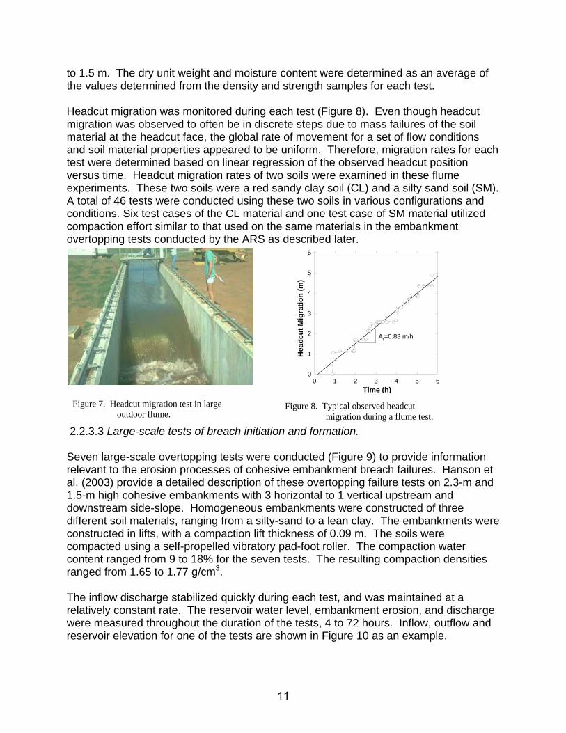
altered. The placement layer thickness was increased to 0.4 m, and the compaction pressure was reduced at a construction height of approximately 3 m. The average resulting compaction density was 1.47 g/cm3. The test inflow, reservoir level, and breach outflow are shown in Figure 5.

2.2.3 Embankment overtopping research – US The Agricultural Research Service (ARS) Hydraulic Engineering Research Unit at Stillwater, Oklahoma has historically conducted studies of the erosional failure processes of grass-lined earth emergency spillways. This research led to a 3-phase earth spillway erosion model that has been incorporated into the USDA Natural Resources Conservation Service (NRCS) SITES computer software. These research results have led to a natural progression of research in the area of embankment overtopping erosion and breach. The following four projects have been undertaken to extend the spillway erosion research into embankment overtopping erosion.

Test Embankment Location

Figure 9. Test site location in Norway downstream of Rosvatn Dam.

Figure 10. Embankment overtopping setup.

0

50

100

150

200

250

300

350

400

450

0 8640 17280 25920 34560 43200 51840Time (sec)

366

367

368

369

370

371

Inflow

Outflow

Reservoir Elevation

Figure 11. Embankment overtopping and breach hydrograph.

9

2.2.3.1 Steep grass and bare earth channel tests An allowable stress design procedure (Temple et al., 1987) for grass-lined channels was developed from large-scale laboratory test data accumulated over the past 60 years. The procedure uses effective stress on the soil for the purpose of predicting incipient failure of the vegetated lining due to movement of the erodible boundary supporting vegetation. Physical model tests to extend the research on vegetation in waterways and spillways to steep embankments were carried out on a 3-m high embankment constructed in the outdoor laboratory (Figure 6) (Hanson and Temple, 2002). After construction of the embankment, six 0.9-m wide channels were cut into the embankment to allow tests to be conducted on individual sections. The slope of the channels was 33% and the soil classified as ML to CL-ML in the Universal Soil Classification System. The embankment was compacted in 0.15 m lifts at and average compaction water content of 12% and specific weight of 1.8 g/cm3. Tests were conducted on green bermudagrass, dormant bermudagrass, green fescue, and bare conditions. Effective overtopping depths for the tests ranged from 0.27 to 0.67 m. Duration of testing was up to 75 hr with mean velocities up to 5 m/s. Additional studies were conducted to evaluate the effect of surface discontinuities on the effectiveness of vegetal protection.

2.2.3.2 Large-scale flume studies of headcut migration Observations of spillway and embankment erosion confirm that the typical failure mode resulting in breach includes movement of a headcut through the hydraulic control section. Headcut advance tests were performed in a 1.8-m wide and 29-m long flume with 2.4-m high sidewalls (Figure 7) (Hanson et al. 2001). The test flume was filled by placing soil in horizontal loose layers 0.15 to 0.20 m thick. A 0.86-m wide vibratory padfoot roller was used to compact each layer, and a hand-held pneumatic compactor was used to compact the soil against the flume walls. Compactive effort and water content were varied from test to test. Prior to testing, a near vertical overfall was preformed at the downstream end of the test section. Overfall heights varied from 0.9 m

Figure 6. Example of steep channel tests.

10

to 1.5 m. The dry unit weight and moisture content were determined as an average of the values determined from the density and strength samples for each test. Headcut migration was monitored during each test (Figure 8). Even though headcut migration was observed to often be in discrete steps due to mass failures of the soil material at the headcut face, the global rate of movement for a set of flow conditions and soil material properties appeared to be uniform. Therefore, migration rates for each test were determined based on linear regression of the observed headcut position versus time. Headcut migration rates of two soils were examined in these flume experiments. These two soils were a red sandy clay soil (CL) and a silty sand soil (SM). A total of 46 tests were conducted using these two soils in various configurations and conditions. Six test cases of the CL material and one test case of SM material utilized compaction effort similar to that used on the same materials in the embankment overtopping tests conducted by the ARS as described later.

2.2.3.3 Large-scale tests of breach initiation and formation. Seven large-scale overtopping tests were conducted (Figure 9) to provide information relevant to the erosion processes of cohesive embankment breach failures. Hanson et al. (2003) provide a detailed description of these overtopping failure tests on 2.3-m and 1.5-m high cohesive embankments with 3 horizontal to 1 vertical upstream and downstream side-slope. Homogeneous embankments were constructed of three different soil materials, ranging from a silty-sand to a lean clay. The embankments were constructed in lifts, with a compaction lift thickness of 0.09 m. The soils were compacted using a self-propelled vibratory pad-foot roller. The compaction water content ranged from 9 to 18% for the seven tests. The resulting compaction densities ranged from 1.65 to 1.77 g/cm3. The inflow discharge stabilized quickly during each test, and was maintained at a relatively constant rate. The reservoir water level, embankment erosion, and discharge were measured throughout the duration of the tests, 4 to 72 hours. Inflow, outflow and reservoir elevation for one of the tests are shown in Figure 10 as an example.

Figure 7. Headcut migration test in large outdoor flume.

0 1 2 3 4 5 60

1

2

3

4

5

6

Hea

dcut

Mig

ratio

n (m

)

Time (h)

Ar=0.83 m/h

Figure 8. Typical observed headcut migration during a flume test.

11

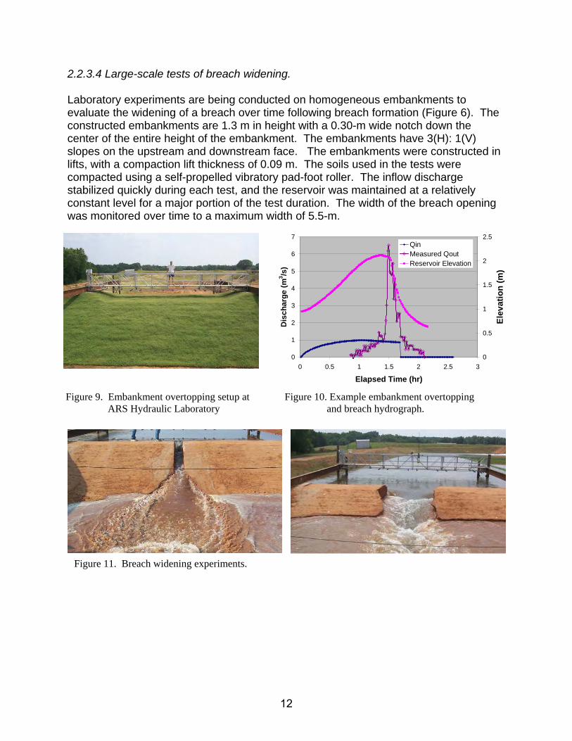
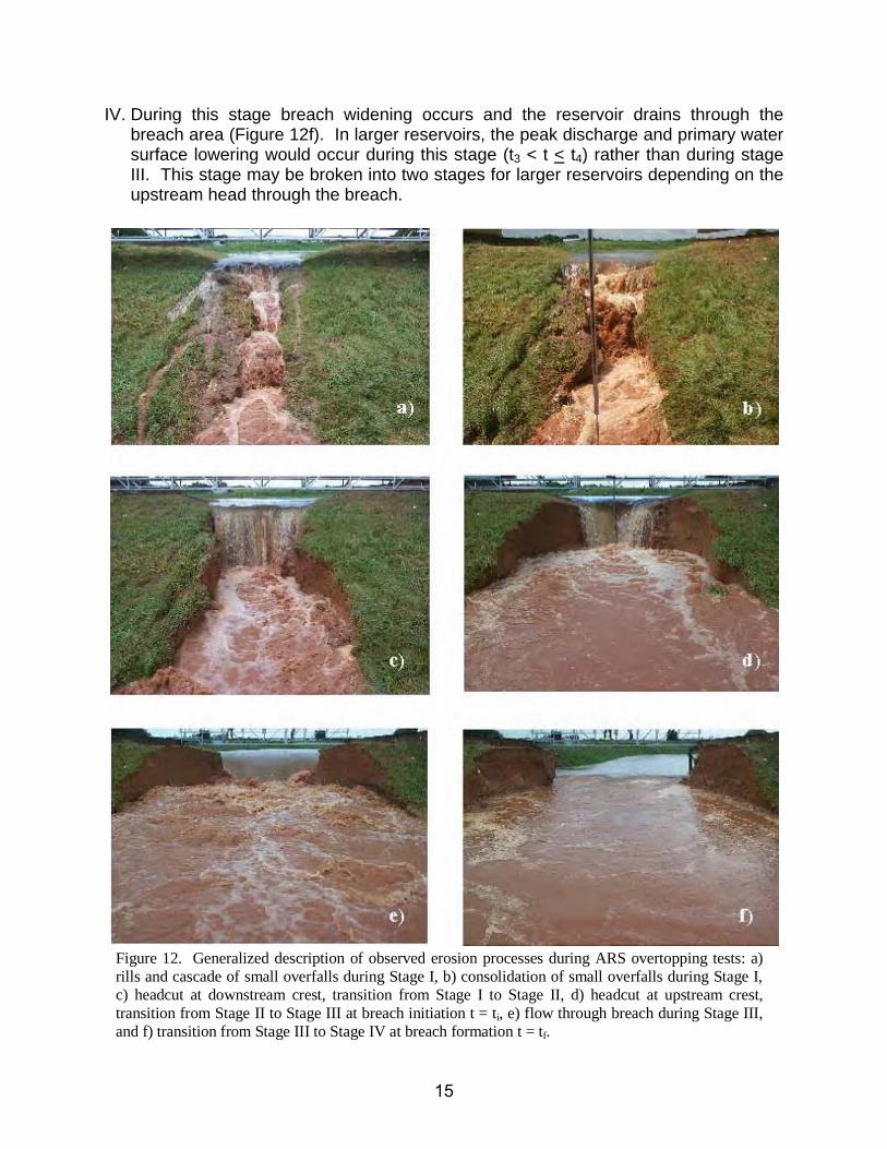
2.2.3.4 Large-scale tests of breach widening. Laboratory experiments are being conducted on homogeneous embankments to evaluate the widening of a breach over time following breach formation (Figure 6). The constructed embankments are 1.3 m in height with a 0.30-m wide notch down the center of the entire height of the embankment. The embankments have 3(H): 1(V) slopes on the upstream and downstream face. The embankments were constructed in lifts, with a compaction lift thickness of 0.09 m. The soils used in the tests were compacted using a self-propelled vibratory pad-foot roller. The inflow discharge stabilized quickly during each test, and the reservoir was maintained at a relatively constant level for a major portion of the test duration. The width of the breach opening was monitored over time to a maximum width of 5.5-m.

Figure 11. Breach widening experiments.

Figure 9. Embankment overtopping setup at ARS Hydraulic Laboratory

0

1

2

3

4

5

6

7

0 0.5 1 1.5 2 2.5 3

Elapsed Time (hr)

Dis

char

ge (m

3 /s)

0

0.5

1

1.5

2

2.5

Elev

atio

n (m

)

QinMeasured QoutReservoir Elevation

Figure 10. Example embankment overtopping and breach hydrograph.

12

2.3 Summary of Results Related to Cohesive Embankment Tests A significant amount of information from these tests has been collected. Tables 2, 3, and 4 provide a summary of data for the tests conducted in the US, UK, and Norway including, embankment geometry, soil properties, and breach parameters. Table 2. Summary of Cohesive Embankment Overtopping Tests.

Embankment Dimensions Notch Dimensions Reservoir Test Series

Height (m)

Section Length

(m)

Crest Width (m)

D.S. Slope

U.S. Slope

BottomWidth (m)

Depth

(m)

Side Slopes

Storage Volume

(m3)

Inflow (m3/s)

US-1 2.3 7.3 3 3:1 3:1 1.83 0.46 3:1 3787 1.0 -2 2.3 7.3 3 3:1 3:1 1.83 0.46 3:1 3975 1.0 - 3 2.3 7.3 3 3:1 3:1 1.83 0.46 3:1 3942 1.0 - 4 1.5 4.9 2 3:1 3:1 1.22 0.30 3:1 4404 1.0 - 5 1.5 4.9 2 3:1 3:1 1.22 0.30 3:1 4552 1.0 - 6 1.5 4.9 2 3:1 3:1 1.22 0.30 3:1 4368 0.33 - 7 2.1 12.2 3 3:1 3:1 8.23 0.30 3:1 4094 1.93 UK-1 0.6 4.0 0.2 2:1 2:1 0.54 0.05 2:1 244 0.02-0.26 -2 0.6 4.0 0.2 2:1 2:1 0.54 0.05 2:1 244 0.02-0.26 -3 0.6 4.0 0.2 2:1 2:1 0.54 0.05 2:1 244 0.03-0.27 -4 0.6 4.0 0.2 2:1 2:1 0.54 0.05 2:1 244 0.02-0.09 -5 0.6 4.0 0.2 2:1 2:1 0.54 0.05 2:1 244 0.10-0.27 -6 0.6 4.0 0.2 1:1 2:1 0.54 0.05 2:1 244 0.03-0.26 -7 0.6 4.0 0.2 3:1 2:1 0.54 0.05 2:1 244 0.02-0.26 N –2 6.0 36 2.0 2.3:1 2.4:1 6.65 0.45 1:1 56000 1-350

Table 3. Summary of Material Properties for Cohesive Embankment Tests.

Classification Parameters1 Compaction Test Series Sand %

>0.105 mm Clay %

<0.002 mm PI2 USCS3 WC4

% γd

5

(g/cm2)US -1 70 5 NP SM 8.7 1.72 - 2 25 26 17 CL 16.4 1.65 - 3 63 6 NP SM 12.1 1.73 -4 67 3 NP SM 11.5 1.73 -5 27 26 16 CL 17.8 1.67 -6 65 6 NP SM 14.5 1.74 -7 64 6 NP SM 11.5 1.77 UK -1 0 43 35 CH 24.6 1.20 -2 0 43 35 CH 23.7 1.20 -3 0 43 35 CH 21.5 1.10 -4 0 43 35 CH 27.9 1.23 -5 0 43 35 CH 27.9 1.23 -6 0 43 35 CH 19.6 1.16 -7 0 43 35 CH 19.2 1.13 N – 2 5 30 13 CL 30.0 1.47 1Tests by USDA-NRCS Soil Mechanics Center. 2PI – Plasticity Index, 3USCS – Universal Soil Classification System, 4WC – water content, 5γd – dry unit weight.

13

Table 4. Embankment overtopping breach results. Breach Values (Following Overtopping) Headcut Migration

Rate, dX/dt DowncuttingRate, dZ/dt

Test Series Breach1 Initiation

Time (sec)

Breach1 Formation Time (sec)

Final Breach

Width (m)

Peak Discharge

(m3/s) Stage II1

(m/hr) Stage III1

(m/hr) Stage III1

(m/hr) US -1 1860 1200 6.9 6.5 7.4 15.7 5.5 -2 >72000 - - - 0.14 - - -3 19200 5990 6.2 1.8 0.68 2.3 1.1 -4 2400 4000 3.3 2.3 7.6 2.4 1.1 -5 >260000 - - - 0.04 - - -6 70320 21960 3.3 1.3 0.23 0.28 0.2 -7 18420 3140 4.5 4.2 1.3 3.1 2.1 UK -1 840 4400 1.83 0.31 0.86 0.90 0.45 -2 840 3670 1.69 0.34 0.86 1.08 0.54 -3 513 1477 2.60 0.53 1.4 2.68 1.34 -4 - - - - 0.26 - - -5 - 11194 1.33 0.28 - 0.36 0.18 -6 212 2829 1.73 0.35 3.40 1.40 0.70 -7 248 1740 2.34 0.43 2.90 2.28 1.14 N –2 6540 566 22.7 390 1.10 49 35 1 Terms for breach initiation, formation, and stages defined in section, “LESSONS LEARNED.” 2.4 Lessons Learned from Cohesive Embankment Breach Tests 2.4.1 Observed erosion processes of cohesive embankments Observations and data recorded during overtopping of the seven ARS embankments testsd, led to a four-stage description of the embankment breach processes (Hanson et al., 2003): I. Flow over the embankment initiates at t = t0. Initial overtopping flow results in sheet

and rill erosion with one or more master rills developing into a series of cascading overfalls (Figure 12a). Cascading overfalls develop into a large headcut (Figure 12b and 12c). This stage ends with the formation of a large headcut at the downstream crest and the width of erosion approximately equal to the width of flow at the downstream crest at t = t1,

II. The headcut migrates from the downstream to the upstream edge of the embankmet crest. The erosion widening occurs due to mass wasting of material from the banks of the gully. This stage ends when the headcut reaches the upstream crest at t = t2 (Figure 12d),

III. The headcut migrates into the reservoir lowering of the crest occurs during this stage and ends when downward erosion has virtually stopped at t = t3 (Figure 12e). Because of the small reservoir size, the peak discharge and primary water surface lowering occurred during this stage, and

14

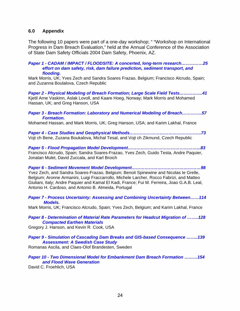
IV. During this stage breach widening occurs and the reservoir drains through the breach area (Figure 12f). In larger reservoirs, the peak discharge and primary water surface lowering would occur during this stage (t3 < t < t4) rather than during stage III. This stage may be broken into two stages for larger reservoirs depending on the upstream head through the breach.

Figure 12. Generalized description of observed erosion processes during ARS overtopping tests: a) rills and cascade of small overfalls during Stage I, b) consolidation of small overfalls during Stage I, c) headcut at downstream crest, transition from Stage I to Stage II, d) headcut at upstream crest, transition from Stage II to Stage III at breach initiation t = ti, e) flow through breach during Stage III, and f) transition from Stage III to Stage IV at breach formation t = tf.

15

Stages I and II encompass the time period of breach initiation up to t = ti, and Stage III encompasses the time period referred to as breach formation t = tf. These stages as described are a generalization of the processes that were observed. These same general processes were observed in the tests conducted in Norway (Figure 13) and the UK. In addition to the observed stages of erosion and headcut formation and migration as one of the dominant erosion processes, other observations included: 1) Vertical or nearly vertical sidewalls during erosion and breach widening in all test cases (Figures 12-14); and 2) Formation of an arch-type weir during breach formation (Figure 14). 2.4.2 Initiation and formation time Wahl (1998) defined breach initiation time as the time that spans from the first flow over the dam to the point of lowering of the upstream embankment crest of the dam and breach formation times as the time that spans from the point of lowering of the upstream embankment crest of the dam to the point at which the upstream face is eroded to full depth of the dam. The breach initiation time can be important in determining hazard downstream, warning time, and evacuation planning. Breach initiation involves stages I and II as described previously. The steep channel vegetation tests indicate that vegetation can increase the length of time for breach initiation and within certain flow durations and stresses the vegetation may prevent breach initiation altogether. Results from embankment overtopping tests at the ARS, HR Wallingford, and Norway also indicate that breach initiation time can be quite lengthy and often greater than breach formation time. Breach initiation times were observed to range from a low of 0.07 to 11.6 times the breach formation time (Table 4). Two of the ARS tests were observed to still be in breach initiation at the end of the tests after overtopping durations of 20 and

Figure 13. Observed headcut erosion during cohesive embankment overtopping test in Norway

Figure 14. Curved weir control section during breach formation during Norway test.

Curved Weir Section

16

72 hours (Table 4). The breach initiation time is dependent on embankment vegetation, material type and placement, embankment geometry, reservoir storage, and discharge. 2.4.3 Rate of erosion and compaction effects Walder and O’Connor (1997) point out the importance of breach erosion rate, in addition to reservoir volume and dam embankment height, for determining peak discharge. Hassan et al. 2004 observed that a decrease in compaction energy and water content of the embankment accelerated the erosion process, which led to higher peak outflow and large final breach width. Erosion rate not only impacts peak discharge and final breach width but also affects the amount of erosion damage, breach initiation time, breach formation time, and rate of breach widening. As an example, headcut erosion is one of the key erosion processes observed during cohesive embankment overtopping (Figure 12). The flume headcut migration tests conducted by the ARS indicate that the rate of headcut migration and breach erosion is impacted by placement compaction energy and water content (Hanson and Cook, 2004). Inspection of a simple headcut migration equation developed by Temple (1992) indicates that the rate of headcut migration dX/dt is a function of the unit discharge q, headcut height H, and C a headcut migration coefficient:

dX/dt = C(qH)1/3 [1] The headcut migration coefficient C is a function of the material properties. A preliminary comparison of calculated C values for the ARS flume and the ARS, HR Wallingford, and Norway embankment test results for Stages I and II is shown in Figure 15. These results indicate: 1) the compaction energy for the ARS flume and ARS embankment tests were equivalent indicating a consistency in C values for these two different test environments; 2) for the six different cohesive soils used in the ARS flume and embankment tests, the C value is dependent on the compaction energy and water content; 3) the compaction water content has a significant effect on the headcut migration coefficient; and 4) the compaction energy used in the construction of HR Wallingford and Norway embankments was significantly less than the compaction energy used in the ARS flume and embankment tests. This difference in compaction energy resulted in a significant shift upward for the results of C, but a similar slope for C versus compaction water content was retained. Integrating the results from the different tests that have been conducted will be important in developing numerical models to predict breaching. One of the key

Water Content %8 9 20 30 4010

C (s

ec)-2

/3

10-5

10-4

10-3

10-2

ARS EmbUK DataNorway ARS Flume

Figure 15. Headcut migration coefficient for flume and embankment test results.

17

requirements in modeling will be the development of approaches to determine appropriate input parameters for identifying processes and predicting erosion rates. 3.0 WORKSHOP The one day workshop was held at the Annual Conference of the Association of State Dam Safety Officials 2004 Dam Safety. The title of the day long workshop was; “Workshop on International Progress in Dam Breach Evaluation.” Ten presentations were included in the workshop. Even though the primary focus of the research interaction described in section 2.0 was on cohesive embankment overtopping and failure testing, data collection, and integration; the workshop included a broader scope of papers. The workshop covered subject matters related to embankment failure and flooding such as: embankment overtopping and failure testing of cohesive, non-ochesive, and rockfill embankments; geophysical measurements of embankments and material property implications related to embankment breach; flood propogation, sediment movement, and embankment dam breach modeling; and risk and uncertainty related to flooding. The broad scope of the workshop reflects not only the concerns in Europe related to dam failures and flooding but also the concerns in the USA. Note: The papers in the workshop do not describe all of the research being conducted

in Europe or the US but provide an overview of the effort and insight into the current state of the science. In order to understand in fuller detail the research being conducted in Europe related to flooding, a network described at the following link http://www.crue-eranet.net/ , has been established. The purpose of the CRUE network is to 1) consolidated European flood research programs, promote best practice and identify gaps and opportunities for collaboration on future research program content. At present it consists of 13 European countries that have been particularly affected by flooding.

3.1 Summary of Workshop Papers (see appendix for actual manuscripts) 3.1.1 Paper 1 –

CADAM / IMPACT / FLOODSITE: A concerted, long-term research effort on dam safety, risk, dam failure prediction, sediment transport, and flooding – Authors: Mark Morris, UK; Yves Zech and Sandra Soares Frazao, Belgium; Francisco Alcrudo, Spain; and Zuzanna Boulalova, Czech Republic.

This paper reviews the research covered in the three European Commission Projects (CADAM, IMPACT, and FLOODSITE). These three projects have resulted in concerted long term research in Europe to investigate 1) breaching of embankments, 2) flood inundation and routing, 3) mechanisms of sediment movement, 4) geophysical methods to assess embankment integrity and 5) uncertainty and risk related to flood defenses and prediction.

18

3.1.2 Paper 2 – Physical Modeling of Breach Formation; Large Scale Field Tests – Authors: Kjetil Arne Vaskinn, Aslak Lovoll, and Kaare Hoeg, Norway; Mark Morris and Mohamed Hassan, UK; and Greg Hanson, USA

This paper describes the large scale physical modeling of embankment erosion and failure due to overtopping and internal erosion. The tests have been conducted on 5 to 6m embankments constructed in the middle of Norway near the town of Mo I Rana. The test site was located about 600 m downstream of the Rossvassdammen Dam which made it possible to control inflow to the test site. A total of 7 field tests were performed on cohesive, and non-cohesive materials (i.e. moraine and rockfill). The structures were failed by overtopping and internal erosion with the purpose of observing erosion processes, rates of erosion, and rates of resulting discharge. One of the key erosion processe observed was headcut development and migration. It was interesting to note that headcutting was even observed in the non-cohesive rockfill structures. 3.1.3 Paper 3 –

Breach Formation: Laboratory and Numerical Modeling of Breach Formation – Authors: Mohamed Hassan, and Mark Morris, UK; Greg Hanson, USA; and Karim Lakhal, France

This paper describes the small scale testing that was conducted on 0.5 to 0.6 m height non-cohesive and cohesive embankments as well as numerical model development and comparisons using the physical model results. A total of 22 laboratory embankment failures tests were conducted. The physical model results indicated the importance of embankment geometry, breach location, erosion processes, erosion rate, and material type and placement on embankment breach. Numerical model results and performance were also compared in this paper. Not all numerical models were compared against all physical model results. 3.1.4 Paper 4 –

Case Studies and Geophysical Methods – Authors: Vojt ch Bene, Zuzana Boukalova, Michal Tesal, and Vojt ch Zikmund, Czech Republic

Results from geophysical measurements at selected locations in the Czech republic are present in this paper. A framework design for a dike breach parameters database is also presented. It is concluded in this paper that a combination of geophysical methods is appropriate for determining preventive repair and maintenance needs of embankments. The suggested combination of geophysical methods fall into three basic categories: 1) rapid testing methods, 2) diagnostic methods, and 3) monitoring methods. 3.1.5 Paper 5 –

Flood Propagation Model Development – Authors: Francisco Alcrudo, Spain; Sandra Soares-Frazao, Yves Zech, Guido Testa, Andre Paquier, Jonatan Mulet, David Zuccala, and Karl Broich

19

This paper provides a review of the main issues and research being conducted concerning flood propagation, model development, and validation. Experimental set-up and data collection for validating the Shallow Water Equations flood routing models described in this paper fall into two types; 1) very simple geometric configurations in which the flooding is idealized and 2) scale physical models of actual topographies. Two of the idealized configurations include a dam break flow in a flume with an isolated building and another with an idealized hillside. One of the scale physical models is a 1:100 scale of a reach of the Alpine River Toce and another physical model described in this paper is of a model city flooding experiment. 3.1.6 Paper 6 –

Sediment Movement Model Development – Authors: Yvez Zech, and Sandra Soares-Frazao, Belgium; Benoit Spinewine and Nicolas Ie Grelle, Belgium; Aronne Armanini, Luigi Fraccarrollo, Michele Larcher, Rocco Fabrizi, and Matteo Giuliani, Italy; Andre Paquier and Kamal El Kadi, France; Fui M. Ferreira, Joao G.A.B. Leal, Antonio H. Cardoso, and Antonio B. Almeida, Portugal

This paper presents aspects of sediment movement modeling related to a flood wave following a dam-break. The difficulty in modeling dam-break flows is that they involve rapid changes and intense rates of transport. This paper reviews physical and numerical modeling of the near-field behavior and far field behavior related to sediment movement following a dam break. 3.1.7 Paper 7 –

Process Uncertainty: Assessing and Combining Uncertainty Between Models – Authors: Mark Morris, UK; Francisco Alcrudo, Spain; Yves Zech, Belgium; and Karim Lakhal, France

This paper identifies the advances that have been made relative to uncertainty associated with breach formation, flood propogation, and sediment movement and the importance to risk management of flood defenses. A methodology is described for combining sensitivity analysis, Monte Carlo analysis and expert judgement to allow assessment of modeling uncertainty and integration of uncertainty between models. 3.1.8 Paper 8 –

Determination of Material Rate Parameters for Headcut Migration of Compacted Earthen Materials – Authors: Gregory J. Hanson, and Kevin R. Cook, USA

This paper recognizes the importance of embankment material properties on embankment erosion and failure. The rate of embankment failure can dramatically impact the rate of water released from a reservoir and the resulting downstream peak flooding and duration of flooding. Headcut development and migration is recognized as one of the key erosion processes related to overtopping of cohesive embankments. Flume test results and observerd impact of material types and placement of the soil materials on rate of headcut migration are discussed in this paper.

20

3.1.9 Paper 9 –

Simulation of Cascading Dam Breaks and GIS-based Consequence Assessment: A Swedish Case Study – Authors: Romanas Ascila, and Claes-Olof Brandesten, Sweden

This paper describes the use and development of an integrated approach in Sweden that looks at dam-break modeling over an entire system including potentially a cascade of dams. A specific study area presented in the paper is a dam cascade situated on the river Lilla Lule Alv in the northern part of Sweden. This study covers eight dams. The methodology covers procedures for data collection and processing, hydraulic modeling, GIS integration and modeling, and consequence analysis and dissemination of the results. This approach enables the simulation of the whole system and provides a better understanding of possible consequences and identified system needs. 3.1.10 Paper 10 - Two Dimensional Model for Embankment Dam Breach Formation

and Flood Wave Generation – Authors: David C. Froehlich, USA This paper describes a two-dimensional depth-averaged breach model including assumptions, inputs, governing equations, formulations, and computation simulation results. The simulations results described in this paper are based on data from the large-scale earthen embankment experimental erosion tests conducted in Norway described in paper 2 of this workshop. 4.0 CONCLUSION

Study of the erosion mechanics of overtopping flow of cohesive embankments in Europe and the US has advanced the science in a number of areas including: vegetation effects, erosion processes, erosion rates, failure timing, breach hydrograph, material type and placement effects, and scaling. There is still much work to be conducted to integrate the work described in this report to continue the formulation of a cohesive embankment breach model. Work, as described in the papers presented in the workshop (Appendix), has begun the development of computational models, and risk analysis based on the physical modeling results. The value of integrating research programs nationally and internationally has been recognized and cooperation is ongoing. Effective integration of this work avoids duplication of research effort and allows ideas and concepts from a wider range of sources to be considered. The Federal Emergency Management Agency through the National Dam Safety Program provided the resources to coordinate the ongoing efforts described in the report for the benefit of the dam safety community.

21

5.0 REFERENCES Costa, J.E. 1985. Floods from dam failures, U.S. Geological Survey Open-File Report

85-560, Denver, Colorado, 54 p. Froehlich, D.C. 1987. Embankment-dam breach parameters. Hydraulic Engineering

Proceedings of the 1987 ASCE National Conference on Hydraulic Engineering, Williamsburg, Virginina, August 3-7, 1987, p. 570-575.

Froehlich, D.C. 1995. Embankment dam breach parameters revisited. Water Resources Engineering, Proceedings of the 1995 ASCE Conference on Water Resources Engineering, San Antonio, Texas, August 14-18, 1995, p. 887-891.

Hanson, G. J. and K. R. Cook. 2004. Determination of material rate parameters for headcut migration of compacted earthen materials. Proceedings from Dam Safety 2004, ASDSO, Inc. CD ROM.

Hanson, G. J. , K. M. Robinson, and K. R. Cook. 2001. Prediction of Headcut Migration Using a Deterministic Approach. Transactions of the ASAE 44(3): 525-531.

Hanson, G. J., and Temple, D. M. 2002. Performance of Bare-Earth and Vegetated Steep Channels Under Long-Duration Flows. Transactions of the ASAE 45(3):695-701.

Hanson, G. J., K.R. Cook, W. Hahn, and S. L. Britton. 2003. Observed erosion processes during embankment overtopping tests. ASAE Paper No. 032066. ASAE St. Joseph, MI.

Hassan, M., M. Morris, G. Hanson, and K. Lakhal. 2004. Breach Formation: Laboratory and Numerical Modeling of Breach Formation. Proceedings from Dam Safety 2004, ASDSO, Inc. CD ROM.

MacDonald, T.C. and J. Langringe–Monopolis. 1984. Breaching characteristics of dam failures. Journal of Hydraulic Engineering, Vol.110(5):567-586.

Morris, M., Y. Zech, S. S. Frazao, F. Alcrudo, Z. Boulalova., 2004. CADAM / IMPACT / FLOODSITE: A concerted, long-term research effort on dam safety, risk, dam failure prediction, sediment transport, and flooding. Proceedings from Dam Safety, 2004, ASDSO, Inc. CD ROM.

Ralston, D.C. 1987. Mechanics of embankment erosion during overflow. Proceedings of the 1987 National Conference on Hydraulic Engineering, Hydraulics Division of ASCE. P. 733-738.

Temple, D. M., K.M. Robinson, A. H. Ahring, and A. G. Davis. 1987. Stability Design of Grass-Lined Open Channels. USDA, ARS, Agriculture Handbook #667.

Temple, D. M. 1992. Estimating Flood Damage to Vegetated Deep Soil Spillways. Applied Engineering in Agriculture, 8(2):237-242. American Society of Agricultural Engineers

Soil Conservation Service (Now NRCS, formerly SCS). 1981. Simplified dam-breach routing procedure. Technical Release No. 66 (Rev. 1), 39p.

Singh V. P. 1996. Dam Breach Modeling Technology. Water Science and Technology Library Volume 17. Kluwer Academic Publishers. Boston. Pp. 242.

Vaskinn, K. A., A. Lovoll, K. Hoeg, M. Morris, G. Hanson, M. A. A. M. Hassan. 2004. Physical Modeling of Breach Formation: Large scale field tests. Proceedings from Dam Safety 2004, ASDSO, Inc. CD ROM.

22

Walder, J.S., and J.E. O’Connor. 1997. Methods for predicting peak discharge of floods caused by failure of natural and constructed earth dams. Water Resources Research, Vol.33(10):10p.

Wahl, T.L. 1998. Prediction of embankment dam breach parameters: A literature review and needs assessment. DSO-98-004. Dam Safety Office, Water Resources Research Laboratory, U.S. Bureau of Reclamation. Denver, CO.

Wahl, T.L. 2001. The uncertainty of embankment dam breach parameter predictions based on dam failure case studies. Proceedings of the USDA/FEMA Workshop Issues, resolutions, and research needs related to embankment dam failure analysis. Oklahoma City, OK.

23

6.0 Appendix

The following 10 papers were part of a one-day workshop; “ “Workshop on International Progress in Dam Breach Evaluation,” held at the Annual Conference of the Association of State Dam Safety Officials 2004 Dam Safety, Phoenix, AZ.

Paper 1 - CADAM / IMPACT / FLOODSITE: A concerted, long-term research……………25

effort on dam safety, risk, dam failure prediction, sediment transport, and flooding.

Mark Morris, UK; Yves Zech and Sandra Soares Frazao, Belgium; Francisco Alcrudo, Spain; and Zuzanna Boulalova, Czech Republic Paper 2 - Physical Modeling of Breach Formation; Large Scale Field Tests…………….41 Kjetil Arne Vaskinn, Aslak Lovoll, and Kaare Hoeg, Norway; Mark Morris and Mohamed Hassan, UK; and Greg Hanson, USA Paper 3 - Breach Formation: Laboratory and Numerical Modeling of Breach…………..57

Formation. Mohamed Hassan, and Mark Morris, UK; Greg Hanson, USA; and Karim Lakhal, France Paper 4 - Case Studies and Geophysical Methods…………………………………………..73 Vojt ch Bene, Zuzana Boukalova, Michal Tesal, and Vojt ch Zikmund, Czech Republic Paper 5 - Flood Propagation Model Development…………………………………………...83 Francisco Alcrudo, Spain; Sandra Soares-Frazao, Yves Zech, Guido Testa, Andre Paquier, Jonatan Mulet, David Zuccala, and Karl Broich Paper 6 - Sediment Movement Model Development…………………………………………98 Yvez Zech, and Sandra Soares-Frazao, Belgium; Benoit Spinewine and Nicolas Ie Grelle, Belgium; Aronne Armanini, Luigi Fraccarrollo, Michele Larcher, Rocco Fabrizi, and Matteo Giuliani, Italy; Andre Paquier and Kamal El Kadi, France; Fui M. Ferreira, Joao G.A.B. Leal, Antonio H. Cardoso, and Antonio B. Almeida, Portugal Paper 7 - Process Uncertainty: Assessing and Combining Uncertainty Between……114

Models. Mark Morris, UK; Francisco Alcrudo, Spain; Yves Zech, Belgium; and Karim Lakhal, France Paper 8 - Determination of Material Rate Parameters for Headcut Migration of ……..128

Compacted Earthen Materials Gregory J. Hanson, and Kevin R. Cook, USA Paper 9 - Simulation of Cascading Dam Breaks and GIS-based Consequence ……..139

Assessment: A Swedish Case Study Romanas Ascila, and Claes-Olof Brandesten, Sweden Paper 10 - Two Dimensional Model for Embankment Dam Breach Formation ………154

and Flood Wave Generation David C. Froehlich, USA

24

CADAM / IMPACT / FLOODSITE

Mark Morris, HR Wallingford UK Mohamed Hassan, HR Wallingford UK

Yves Zech, UCL, Belgium Sandra Soares Frazão, UCL, Belgium

Francisco Alcrudo, UDZ, Spain Zuzanna Boukalova, Geo Group, Czech Republic

Abstract In the EU, the asset value of dams and flood defence structures amounts to billions of Euro. These structures include, amongst others, concrete and embankment dams, tailing dams, flood banks, dikes, etc. Many large dams in Europe are located close to centres of population and industry and the consequences of catastrophic failure of one of these structures would be far worse than most other types of technological disaster. To manage and minimise risks effectively, it is necessary to be able to identify hazards and vulnerability in a consistent and reliable manner, to have good knowledge of structure behaviour in emergency situations, and to understand the potential consequences of failure in order to allow effective contingency planning for public safety. This has led to concerted long term research in Europe (including the CADAM, IMPACT, and FLOODsite projects) to reduce uncertainty in predicting extreme flood conditions and improve predictions of risk due to these structures. The specific objectives of the research described in this paper and the following sessions are to advance scientific knowledge and understanding, and develop predictive modelling tools and methods in a number of areas including: (1) breaching of embankments, (2) catastrophic inundation, (3) mechanisms of sediment movement and (4) embankment integrity assessment through the use of geophysical techniques.

What are CADAM, IMPACT and FLOODSITE? The European Commission funds multiple, wide ranging programmes of research and development work aimed at improving the efficiency and quality of life in Europe. Research programmes are typically aimed at addressing European, rather than national issues. Research funding is normally to the extent of 50% for commercial organisations so as to encourage integration and support from industry, which in turn helps to ensure the value of the research. CADAM, IMPACT and FLOODSITE are all projects funded by the Commission that address different aspects of flood risk management.

CADAM (Concerted action on dambreak modelling) was completed in 2000 and, amongst other results, provided prioritised recommendations for research in the field of dambreak analysis to improve the reliability of predictions. CADAM did not fund new research work, but provided a mechanism for researchers and practitioners to meet, exchange information and to some extent, co-ordinate existing national research work. The value of funding for CADAM was ~ €250K. IMPACT (Investigation of extreme flood processes and uncertainty) is a 3-year project under the EC 5th framework programme that finishes in November 2004. IMPACT addresses a number of the key issues that were highlighted by the

Paper - 1

25

CADAM project. The value of work undertaken by IMPACT is ~€2.6M. FLOODsite (Integrated flood risk analysis and management methodologies) is a new project funded under the EC 6th framework programme integrating a wide range of work, undertaken by 36 different partners drawn from 13 countries. The value of work funded is ~€14M. The focus of work under FLOODsite is on flood risk management in general, whilst CADAM and IMPACT specifically address dambreak or extreme flood related issues. Nevertheless, there are aspects of research under the FLOODsite project that are of continuing interest to the dams industry.

The CADAM Concerted Action Project

Members of the CADAM project team comprised researchers and industrialists from across Europe who had an interest in the various aspects of dam-break modelling. The CADAM project team aimed to: • exchange dam-break modelling information between participants: Universities <=>

Research organisations <=> Industry • promote the comparison of numerical dam-break models and modelling procedures with

analytical, experimental and field data. • promote the comparison and validation of software packages developed or used by the

participants. • define and promote co-operative research.

The project was funded as a concerted action by the European Commission, formally commenced in February 1998 and ran for a period of two years. The principal focus of the Concerted Action was a series of expert meetings and workshops, each of which considered a particular topic (e.g. breach formation, flood routing, risk analysis etc). The performance of various numerical models was assessed throughout by comparison under analytical and physical model tests cases and finally against real dam break data. Detailed information relating to the project may be found at www.hrwallingford.co.uk/projects/CADAM). Findings and Recommendations

The final report from CADAM (available on the CADAM website) drew some 31 specific conclusions and identified a series of areas where further research and development was needed to improve the reliability and accuracy of dambreak analysis. A number of these priority areas form the basis for the IMPACT project research programme. These included:

Breach Formation Modelling:

Considerable uncertainty related to the modelling of breach formation processes was identified and the accuracy of existing breach models considered very limited. Research was recommended in a number of areas including:

1. Structure failure mechanisms 2. Breach formation mechanisms 3. Breach location

Debris and Sediments:

It was identified that the movement of debris and sediment can significantly affect flood water levels during a dambreak event and may also be the process through which

Paper - 1

26

contaminants are dispersed. A clear need to incorporate an assessment of these effects within dambreak analyses was identified in order to reduce uncertainties in water level prediction and to allow the risk posed by contaminants, held for example by tailings dams, to be determined. Flow modelling:

The following research areas relate to the performance of flow models and the accuracy of predicted results:

1. Performance of Flow Models 2. Modelling Flow Interaction with Valley Infrastructure 3. Valley Roughness 4. Modelling Flow in Urban Areas

Other research priorities were identified under the headings of database needs and risk / information management. These are not detailed here, but may be found in the CADAM final report.

The IMPACT Project

The IMPACT project addresses the assessment and reduction of risks from extreme flooding caused by natural events or the failure of dams and flood defence structures. The work programme is divided into five main areas, addressing issues raised by the CADAM project. Research into the various process areas is undertaken by groups within the overall project team. Some work areas interact, but all areas are drawn together through an assessment of modelling uncertainty and a demonstration of modelling capabilities through an overall case study application. The IMPACT project provides support for the dam industry in a number of ways, including: • Provision of state of the art summaries for capabilities in breach formation modelling,

dambreak prediction (flood routing, sediment movement etc) • Clarification of the uncertainty within existing and new predictive modelling tools (along with

implications for end user applications) • Demonstration of capabilities for impact assessment (in support of risk management and

emergency planning) • Guidance on future and related research work supporting dambreak assessment, risk

analysis and emergency planning

The core of this paper provides an introduction to the work being undertaken in each of the IMPACT work packages (WPs). Each of these programmes is also detailed under a separate paper in this workshop and more detailed information on all research may be found via the project website at www.impact-project.net. The WPs comprise: WP2: Breach formation WP3: Flood propagation WP4: Sediment movement WP5: Uncertainty analysis WP6: Geophysics and data collection

Paper - 1

27

WP2: Breach Formation Overview of breach work programme aims and objectives

Existing breach models have significant limitations (Morris & Hassan, 2002). A fundamental problem for improving breach models is a lack of reliable case study data through which failure processes may be understood and model performance assessed. The approach taken under IMPACT was to undertake a programme of field and lab work to collate reliable data. Five field tests were undertaken during 2002 and 2003 using embankments 4-6m high. A series of 22 laboratory tests were undertaken during the same period, the majority at a scale of 1:10 to the field tests. Data collected included detailed photographic records, breach growth rates, flow, water levels etc. In addition, soil parameters such as grading, cohesion, water content, density etc. were taken. Both field and lab data were then used within a programme of numerical modelling to assess existing model performance and to allow development of improved model performance.

Current position of research All field and laboratory modelling work has now been completed. The tests undertaken comprised: • Field Test #1 6m homogeneous, cohesive embankment.

(D50 ≈ 0.01mm, <15% sand, ~25% clay); overtopping. • Field Test #2 5m homogeneous non-cohesive embankment (D50 ≈ 5 mm, <5 % fines);

overtopping. • Field Test #3 6m composite embankment (rockfill with moraine core); overtopping. • Field Test #4 6m composite embankment (rockfill with moraine core); piping. • Field Test #5 4m homogeneous embankment (moraine); piping. • Lab Series #1 This series of 9 tests was based around Field Test #2 at a scale of 1:10.

The test material was non-cohesive with variation in material grading, embankment geometry and breach location (side breach).

• Lab Series #2 This series of 8 tests was based around Field Test #1 at a scale of 1:10. The test material was cohesive, with two different materials used, along with different embankment geometry, compaction effort and moisture content.

• Lab Series #3 This series of 5 tests was based around the initiation of pipe formation for Field Test #5.Test data was used to develop reliable failure mechanisms for the field tests. Tests were also undertaken on 1m3 samples of embankment taken from flood defences in the UK.

In conjunction with the field and laboratory tests and data collection an extensive

programme of numerical model testing has been undertaken. Some core objectives of this component of work included: • Identification of more reliable modelling approaches for simulating breach formation • Assessment of the level of uncertainty of current breach modelling techniques • Incorporation of knowledge gained from the field and laboratory tests into existing modelling

tools

Paper - 1

28

Figure 1 Field and laboratory breach tests Modelling was undertaken by members of the IMPACT Team plus additional

organisations internationally. Modelling was first undertaken without access to the field or lab data, and subsequently with access. In this way the performance of models and modellers may be assessed objectively – which more closely matches the conditions under which modellers are typically asked to predict embankment failure. Analysis of the modelling results highlighted some interesting facts and features. Some of these are listed below. All are explained in more detail in the associated paper on breach formation (Hassan et al). • The laboratory tests highlighted the effect that variation in soil parameters / embankment

condition could have on the breach formation process. For example, varying compaction effort and / or changing moisture content, particularly for cohesive materials, could change the erodibility and hence rate and nature of breach growth by an order of magnitude. It was noticeable that very few breach models included these parameters and hence would struggle to reproduce the true embankment behaviour.

• Whilst some models appeared to predict the flood hydrograph reasonably well for some test conditions, all models either over or under predicted the breach growth rate and dimensions. This suggests that prediction of the basic physical growth processes in conjunction with flow calculation is not undertaken accurately. An observation that supports this is the fact that most models predict a critical flow point within the body of the embankment and hence a flow area based upon breach body width. However, both field and laboratory tests often show the growth of curved flow control sections which move upstream out of the breach body and the flow erodes material from the upstream slope.

• Variation in embankment geometry such as slope from 1:3 to 1:2 or 1:4 appears to have little impact on the breach growth process. However, variation in breach location from the centre of an embankment to the side, where lateral growth is restricted in one direction, does have a noticeable effect. This should be taken into consideration when using data to validate models such as from the Teton failure, which was a breach event adjacent to an abutment. It is also relevant in the case of planning breach growth through a landslide generated embankment. Initiating failure adjacent to an abutment will limit the rate of breach growth and hence the rate of flooding downstream.

• An average accuracy of perhaps ±50% may be attributed to many models (broadly considering timing, peak discharge etc). Models simulating aspects of embankment soil behaviour (e.g. slope stability, failure etc.) appeared to show better performance with an indicative accuracy reaching perhaps ±20%.

Paper - 1

29

Future Direction of Research At the time of writing, analysis of the field, laboratory and numerical modelling data is still to be completed, along with the consideration of scale effects between field and laboratory data. A further area of work investigating factors affecting breach location in long fluvial flood defence embankments is also underway. Results and conclusions from a breach review workshop held at Wallingford in April 2004 will be made available. Research work will continue in this area beyond the completion of the IMPACT project through work packages in the FLOODsite project. It is anticipated, however, that the emphasis of analysis under FLOODsite will shift from breach formation (IMPACT) to breach initiation, so helping to enhance our overall ability to predict and ultimately prevent breach formation occurring.

WP 3: Flood Propagation Overview and objectives

The objective of this area of work is to improve our understanding of the dynamics of a catastrophic (extreme) flood and to improve our propagation modelling capability. Four partners are involved in this area, namely the Université Catholique de Louvain (Belgium), CEMAGREF (France), CESI (formerly ENEL) and the University of Zaragoza (Spain). The scope is broadly divided into two areas; urban flooding and flood propagation in natural topographies. General objectives of the work package are to: • identify dam-break flow behaviour in complex valleys, around infrastructure and in urban

areas ( i.e. gain insight into flood flow characteristics) • collect flood propagation and urban flooding data from scaled laboratory experiments that

can be used for development and validation of mathematical models • adapt and develop modelling techniques for the specific features of high intensity floods,

like those induced by the failure of man made structures • perform mathematical model validation and benchmarking, compare different modelling

techniques and identify best approaches including the assessment of accuracy • develop guidelines and appropriate strategies concerning modelling techniques for the

reliable prediction of flood effects • identify, select and document a real flood event affecting an urban area to be used as a

case study where modelling techniques and lessons learned can be applied and tested Current position

To achieve these goals a combination of desk work, laboratory experiments, field work and computer modelling has been undertaken.

The mathematical description of extreme flood flows has been tackled on the basis of the non-linear shallow water equations. Issues like non-linear convective transport, the formation of travelling waves (bores and hydraulic jumps), the forcing due to bottom and bank reaction forces (as included in the source terms of the equations of motion) and wetting and drying problems are key issues in devising the appropriate computer model.

As regards modelling of flood propagation in a city, several strategies have been investigated. A simple one-dimensional model of a city with the streets modelled as water channels has proven effective despite its simplicity. Limitations concern model applicability at wide junctions such as squares etc. Also important two-dimensional features of the flow are often lost, as happens with wave reflections and expansions around building corners. Another technique referred to as bottom elevation, represents buildings and obstacles to flow as abrupt

Paper - 1

30

elevations of the bed function within a two-dimensional model. This is easy to set up but the numerical method must be robust enough to accommodate this sort of singular source term forcing. Another simple technique analysed entailed increasing the roughness coefficient of the area where buildings or obstructions were located. Finally, the highest level of detail can be attained, at least in theory, by careful two-dimensional meshing of the streets and other city areas prone to flooding.

The aim of the experimental work was to provide an insight into understanding key flow features and to provide data under controlled, reproducible conditions that can be used for computational model validation and improvement. Two types of laboratory experiment at a scaled down geometry have been conducted for urban flooding; one devoted to the study of the flow structure around a single building (front impingement and reflection, refraction etc.) and the other to overall flood-city interaction in which a model city in a scaled down (1:100) valley was subjected to a simulated flood event. The data obtained have been used to set up two benchmark sessions against which computer models have been tested, firstly in a blind phase and then followed by the release of experimental data to allow for model tuning.

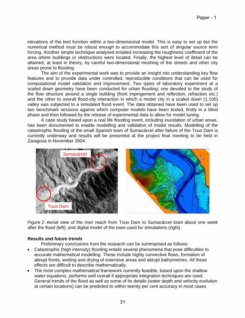
A case study based upon a real life flooding event, including inundation of urban areas, has been documented to enable modelling and validation of model results. Modelling of the catastrophic flooding of the small Spanish town of Sumacárcel after failure of the Tous Dam is currently underway and results will be presented at the project final meeting to be held in Zaragoza in November 2004.

Figure 2: Aerial view of the river reach from Tous Dam to Sumacárcel town about one week after the flood (left); and digital model of the town used for simulations (right).

Results and future trends

Preliminary conclusions from the research can be summarised as follows: • Catastrophic (high intensity) flooding entails several phenomena that pose difficulties to

accurate mathematical modelling. These include highly convective flows, formation of abrupt fronts, wetting and drying of extensive areas and abrupt bathymetries. All these effects are difficult to describe mathematically.

• The most complex mathematical framework currently feasible, based upon the shallow water equations, performs well overall if appropriate integration techniques are used. General trends of the flood as well as some of its details (water depth and velocity evolution at certain locations) can be predicted to within twenty per cent accuracy in most cases

Tous Dam

Sumacárcel

Paper - 1

31

when the flood characteristics (inflow hydrograph and timing etc …) and bathymetry data are well known.

• However important details of the flood may be completely lost when strong deviations from the model equations appear (strong vertical accelerations, high curvature of the streamlines etc…), when the spatial resolution is not enough to precisely describe the geometry or when the flood characteristics are not well known.

Spatial resolution is likely to be a problem when urban areas are to be treated at the same time as propagation of the flood down a natural valley or open terrain. As a general conclusion it can be said that careful validation initiatives like the ones

represented by the Impact project, in particular involving real life data, are still needed to assess the accuracy and uncertainty of present day models and hopefully improve our modelling capabilities.

WP4: Sediment Movement

Overview of WP4 work-programme aims and objectives The “Sediment movement” IMPACT work package explores the field of dam-break

induced geomorphic flows. In a number of ancient and recent catastrophes, floods from dam or dike failures have induced severe soil movements in various forms. Other natural hazards also induce such phenomena: glacial-lake outburst floods and landslides resulting in an impulse wave in the dam reservoir or in the formation of natural dams subject to major failure risk. In some cases, the volume of entrained material can reach the same order of magnitude (up to millions of cubic meters) as the initial volume of water released from the failed dam.

The main goal of work package is to gain a more complete understanding of geomorphic flows and their consequences on the dam-break wave. Dam-break induced geomorphic flows generate intense erosion and solid transport, resulting in dramatic and rapid evolution of the valley geometry. In counterpart, this change in geometry strongly affects the wave behaviour and thus the arrival time and the maximum water level, which are the main characteristics to evaluate for risk assessment and alert organisation.

Near-field and far-field behaviour

Depending on the distance to the broken dam and on the time elapsed since the dam break, two types of behaviour may be described and have to be understood and modelled.

In the near field, rapid and intense erosion accompanies the development of the dam-break wave. The flow exhibits strong free surface features: wave breaking occurs at the centre (near the location of the dam), and a nearly vertical wall of water and debris overruns the sediment bed at the wave forefront, resulting in an intense transient debris flow. However, at the front of the dam-break wave, the debris flow is surprisingly not so different as a uniform one. An important part of the work program was thus devoted to the characterisation of the debris flow in uniform conditions.

Behind the debris-flow front, the behaviour seems completely different: inertial effects and bulking of the sediments may play a significant role. Surprisingly, such a difficult feature appears to be suitably modelled by a two-layer model based on the shallow-water assumptions and methods. The work package included experiments, modelling and validation of this near-field behaviour.

Paper - 1

32

In the far field, the solid transport remains intense but the dynamic role of the sediments decreases. On the other hand dramatic geomorphic changes occur in the valley due to sediment de-bulking, bank erosion and debris deposition. Experiments, modelling and validation of the far-field behaviour composed he last part of the work package.

Current position of research

It appears that one of the most promising approaches of the near-field modelling is a three-layer description (Fig. 3). Three zones are defined: the upper layer (hw) is clear water while the lower layers are composed of a mixture of water and sediments, the upper part of this mixture (hs) being in movement.

In the frame of shallow-water approach, it is possible to express the continuity of both the sediments and the mixture and also the momentum conservation with the additional assumption that the pressure distribution is hydrostatic in the moving layers, which implies that no vertical movement is taken into consideration:

Figure 3. Assumptions for mathematical description of near-field flow

Comparisons and validation were carried out from experimental data on idealised dam-

break: typically, horizontal beds composed of cohesionless sediments saturated with water extending on both sides of an idealised "dam", with various sediment and water depths.

For the far field, special attention was paid to the modelling of the bank behaviour. The bank failure mechanism was observed and modelled, taking into account the specific performance of eroded / deposed material in emerged / submerged conditions.

The far-field experiments consisted in a dam-break flow in an initially prismatic valley made of erodible material, evidencing the bank erosion, the transport of the so-deposed material, and the genera widening of the valley.

Results and future direction of work

Experimental results, obtained at the University of Louvain (Belgium) were proposed as a benchmark to various partners: University of Louvain (Belgium), University of Trento, Cemagref (France) and Technical University of Lisbon (Portugal). Fig. 4 presents a comparison between experimental observation and the model presented above.

Figure 4. Comparison between experiments and numerical results, 1 s after the dam break

Paper - 1

33

It appears that some characters of the movement are well modelled, such as the jump at the water surface, the scouring at the dam location, the moving layer thickness. The modelled front is ahead but this advance appears constant, which implies that the front celerity is correctly estimated.

Also for the far-field behaviour and the valley widening, the models at this stage can produce valuable results to compare with experimental data from idealised situations.

But it is suspected – and this is general conclusion for the “Sediment movement” work package – that we are far from a completely integrated model able to accurately simulate a complex real case. A tentative answer to this could probably be given from the results of real-case benchmark regarding the Lake Ha!Ha! dike break occurred in Quebec in July 1996. The first results of this benchmark will be available after the last IMPACT meeting to be held in Zaragoza, Spain, in November 2004.

WP 5: Uncertainty Analysis

The objective of this work package was to try and identify the uncertainty associated with the various components of the flood prediction process; namely uncertainty in breach formation, flood routing and sediment transport models. In addition, to demonstrate the effect that uncertainty has on the overall flood prediction process through application to a real or virtual case study and to consider the implications of uncertainty in specific flood conditions (such as water level, time of flood arrival etc.) for end users of the information (such as emergency planners). The scope of work under IMPACT does not allow for an investigation of uncertainty in the impact of flooding or in the assessment and management of flood risk.

The challenge of assessing overall modelling uncertainty is complicated by the need to assess uncertainty within two or more models, to somehow transfer a measure of uncertainty between these models and to develop a system that allows for the different complexities of the various models. Two basic approaches were adopted, namely sensitivity analysis and Monte Carlo analysis. However, whilst a breach formation model may be able to run hundreds or thousands of simulations within a period of hours, it is unrealistic to assume that a complex 2D flood propagation model can undertake a similar process without undertaking weeks or months of analysis. A compromise solution was adopted for IMPACT that combines sensitivity analysis, Monte Carlo simulation and expert judgement. Whilst this approach may provide an estimate of uncertainty which contains a degree of subjectivity (expert judgement) it also provides a mechanism that is achieved relatively simply and provides a quick indication of potential uncertainty.

At the time of writing, the approach had been tested using the HR Breach model only. The steps undertaken included: • Sensitivity analysis of the model to a range of model parameters (implicit within this is

expert judgement on selection of appropriate and realistic ranges for parameter variation) • Prioritisation of the modelling parameters to identify those with the greatest effect on

modelling results • Selection of the top three parameters for Monte Carlo analysis (implicit within this is the

selection of a probability distribution function for each parameter, again based upon judgement)

• Analysis of results from 1000 model runs; selection of upper, mid and lower scenarios leading to a comparison between the base run (best estimate of model with chosen

Paper - 1

34

modelling parameters) and the uncertainty analysis upper, mid and lower estimates Table 1 shows analysis of results from 44 model runs to assess model sensitivity to various modelling parameters. This analysis considers only peak discharge. Figure 5 then shows the distribution of model results from the Monte Carlo analysis (based on peak discharge) and specific flood hydrographs representing base, upper, mid and lower scenarios. Table 1: Sensitivity of the peak outflow to the different input parameters

Figure 5: Probability distribution of peak outflow and selected upper, mid and lower scenarios

These results start to give an indication of the uncertainty within the overall flood prediction process. Certainly for breach peak discharge, the suggested realistic range (in this case) is at least ~±30% for peak discharge. However, it is interesting to note that the base run, which represents the experts best judgement in this case, is within 10% of the observed peak discharge. It remains to be seen within the IMPACT project how this band of uncertainty translates through a flood propagation model to uncertainty within the prediction of flood water levels lower in the valley. Whilst attenuation of the flood hydrograph along the valley will tend to reduce the band of uncertainty in water level prediction, the addition of uncertainty within the flood propagation model itself will tend to increase the uncertainty in water level prediction.

Future Direction of Work During the summer of 2004 further analysis will be undertaken to link propagation of breach and flood routing uncertainty, leading to an overall prediction of uncertainty within the estimation of flood water levels lower in the valley.

0

50

100

150

200

250

0 1000 2000 3000 4000 5000 6000Time (s)

Flow

(m

^3/s

)

Lower

Meduim

Upper

Base Run

Measured Peak Outflow

0-65

70-7

5

80-8

5

90-9

5

100-

105

110-

115

120-

125

130-

135

140-

145

150-

155

160-

165

170-

175

180-

185

190-

195

200-

205

210-

215

220-

225

230-

235

240-

245

250-

255

260-

265

270-

275

280-

285

290-

295

New0.00

10.00

20.00

30.00

40.00

50.00

60.00

Freq

uenc

y

Peak outflow ranks (m^3/s)

Peak outflow

5% 50% 95%

Paper - 1

35

WP6: Geophysical Investigation This 2-year module of work was added to the IMPACT project through a programme to

encourage wider research participation with Eastern European countries. The work comprises two components; (1) review and field testing of different geophysical investigation techniques and (2) collation of historic records of breach formation.

The objective of the geophysical work is to develop an approach for the ‘rapid’ integrity assessment of linear flood defence embankments. This aims to address the need for techniques that offer more information than visual assessment, but are significantly quicker (and cheaper) than detailed site investigation work. Research is being undertaken through a series of field trial applications in the Czech Republic at sites where embankments have already been repaired and at sites where overtopping and potential breach is known to be a high risk.

The objective of collecting breach data is to create a database of events that includes as much information as possible relating to the failure mechanisms, local conditions, embankment material and local surface materials. Analysis may then be undertaken to identify any correlation between failure mode, location and embankment material, surface geology etc. Geophysics and Data Collection

Geophysical methods may be used in several variants, most commonly in the surface variant (measurement is performed directly on the earth surface), in the underground variant (in the drills, adits, cellars, etc.) and in the variant of remote monitoring from aeroplanes, satellites, etc. (so-called remote sensing).

During a survey for either hydrogeological, engineering-geological, or geotechnical purposes, it is necessary to select an appropriate combination of these approaches and methodology for the field works. Likewise, it is necessary to understand the relationship between measured physical properties of rocks and parameters that have to be measured or indirectly determined. From the principle point of view, geophysical methods are considered to be indirect methods, because they substitute direct field works such as drilling, excavation etc. Thus, they may significantly save both time and money in comparison and / or combination with direct methods. The main contribution of geophysical methods consists, therefore, in getting higher quality, more extensive and more reliable background information for further survey works. During their application, it is necessary to remain flexible in selecting the most appropriate methods for the site, by working in stages the most effective approach, both scientifically and financially, may be developed.

The key to success in utilising results of geophysical methods is in attaining close co-operation of geophysicists with specialists in hydrogeology and engineering geology. The aim of geophysical testing measurements within the IMPACT project is to investigate and confirm the possibility of using these non-destructive methods in assessing the description and state of existing flood defence dikes. In particular, the rapid assessment of long lengths of flood defence embankment. Geophysical measurements have been conducted on a number of pilot sites within the IMPACT study utilising the following geophysical methods: • geoelectric methods

resistivity profiling (RP), self potential method (SP), multielectrode method (MEM), electromagnetic frequency method (EFM)

• seismic methods shallow seismic method (SSM), seismic tomography (ST), multi-channel analysis of seismic waves (MASW)

Paper - 1

36

• microgravimetric methods • GPR methods • geomagnetic survey, gamma-ray spectrometric survey Current position of research

Geophysical tests and the monitoring of dikes have demonstrated the possibility of developing and subsequent application of specific geophysical technology that could be utilised for a “rapid integrity assessment“ approach. The proposed approach is based upon the use of modified apparatus GEM-2. To finalise this approach it is necessary to collect verification data within the defined catchment, and to verify performance by supplementary methods (multi-electrode method ARS-200, method of spontaneous resistance polarisation – SRP, etc.). If successful, the new geophysical monitoring system should help catchment management and organisation through: • quick testing measurement – its purpose is to provide a basic description of dike

materials and structures and to delimit quasi-homogeneous blocks and potentially hazardous segments. Repeated quick testing measurement data will be stored in the database, allowing us to analyse long-term changes of the dike condition.

• diagnostic measurement for a detailed description of problematic and disturbed dike segments – it serves for optimal repair planning

• monitoring measurement of changes of geotechnical parameters – it serves for repair quality control and for observation of earth structures ageing processes, etc.

Results and conclusions so far

The IMPACT monitoring and tests show that with expert application of geophysical methods we can better describe the real state of a dike. We expect that a proposed combination of geophysical methods would supplement other surveys and activities performed during maintenance (analysis of aerial and satellite photographs, inspection walks). We anticipate proposing a convenient methodology for embankment integrity assessment.

Future direction of work

At the present time, we are striving to prepare a programme of work for the year 2005 and 2006. This programme should cover regular monitoring of dikes in the catchment of Odra or Morava river, and the creation of a database with data measured by modified GEM-2 equipment. In problematic sections (changes of homogeneity of dikes) basic data should be complemented with data obtained by the more precise measurements performed by detail geo-electrical method ARS-200. Assessment of this database will enable us to determine the effectiveness and success of this methodology based on the fast preliminary measurement by GEM-2. This methodology should (together with other supplementary and more precise methods) serve to provide a fast and inexpensive check on flood defence embankments, allowing specific changes in their state with time to be identified (i.e. systematic monitoring of dikes by modified GEM-2 should be used for evaluation of weak places in the dikes, where failure could occur in case of overspill). In future, this fast and non-destructive geophysical method could make operation of water-management bodies within the catchment more effective, and assure early prevention of dike failure. Regular measurements of the dike state could enable estimation of risk of the dike failure, under the various hydrological conditions and plan early and effective repairs of embankments in selected sections. This method can be used for dikes up to about 10 m high of any length.

Paper - 1

37

Where from here? The IMPACT project has made significant advances in science in a number of areas but work is still to be implemented during the summer of 2004 in order to pull together and demonstrate this new knowledge. The Tous Dam failure (Spain) and Lake Ha! Ha! failure (Canada) will be used as case studies to demonstrate modelling capabilities in breach, propagation, sediment movement and uncertainty analysis. Final reporting of this work will be made through a 4th and final project workshop to be held in Zaragoza, Spain on 4-5 November 2004. Information will also be posted via the project website (www.impact-project.net). The nature of the work undertaken and the type of funding from the EC (50%) means that much of the research work has also been integrated with existing national or organisation research projects. Within the UK, the research is meshed within a wider national programme of work funded by the government. Consequently, uptake of knowledge occurs through these links and, where appropriate, continuation of the research. The concept and potential value of integrating research programmes, both nationally and internationally, is now being recognised. Effective integration of work avoids duplication of research effort and allows ideas and concepts from a wider range of sources to be considered. Building on best practice and experience from around the world has to be a more beneficial for all partners than remaining isolated in approach!

Within the last few years, real integration of research programmes can be seen nationally and internationally. This has probably been prompted by the growing use of the Internet as a means of disseminating information. For example, within the UK there are three major programmes of work for which full integration is being attempted. These programmes will run during the coming 3-5 years and comprise: • Environment Agency / Defra national flood defence programme (applied research in field of

flood risk management) [See www.defra.gov.uk/environ/fcd/default.htm] • EPSRC / EA / Defra Flood Risk Management Research Consortium (FRMRC) programme

(academic research programme) [See www.floodrisk.org.uk] • EC FLOODsite Project (processes through to implementation for flood risk management)

[See www.floodsite.net] The FLOODsite Project

The FLOODsite project addresses a wide range of issues dealing with flood risk management. The research programme structure is shown by Figure 6 and covers activities from research into specific processes, through flood risk management, integration of tools, pilot site application and development, training, dissemination and networking. FLOODsite is the European Commission project addressing flood risk management.

The scope of FLOODsite is such that it is not possible to detail the programme here.

However, it should be noted that issues of direct relevance to the dams industry such as breach initiation, flood inundation, integrated modelling and decision support tools, emergency planning tools, vulnerability, social and economic impacts are included within the programme of work. The European Commission has also recognised the value of integrating research from around the world. Under FP6, research projects may include partners from outside of the EC – such as the United States. Such a change in approach has not yet been widely recognised by European researchers, and uptake of funds to date has been limited. Opportunities exist here! For more information on European research initiatives see the Cordis website at

Paper - 1

38

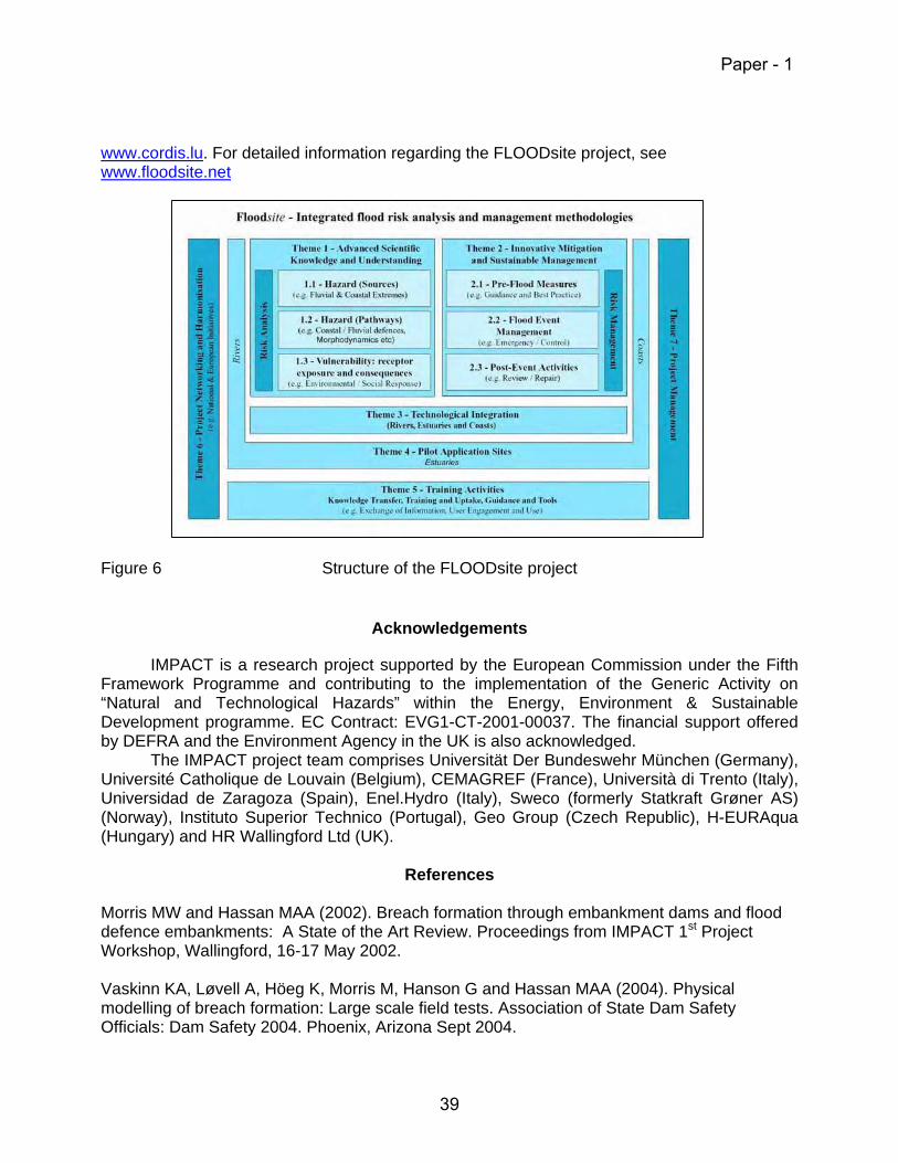
www.cordis.lu. For detailed information regarding the FLOODsite project, see www.floodsite.net

Figure 6 Structure of the FLOODsite project

Acknowledgements

IMPACT is a research project supported by the European Commission under the Fifth Framework Programme and contributing to the implementation of the Generic Activity on “Natural and Technological Hazards” within the Energy, Environment & Sustainable Development programme. EC Contract: EVG1-CT-2001-00037. The financial support offered by DEFRA and the Environment Agency in the UK is also acknowledged.

The IMPACT project team comprises Universität Der Bundeswehr München (Germany), Université Catholique de Louvain (Belgium), CEMAGREF (France), Università di Trento (Italy), Universidad de Zaragoza (Spain), Enel.Hydro (Italy), Sweco (formerly Statkraft Grøner AS) (Norway), Instituto Superior Technico (Portugal), Geo Group (Czech Republic), H-EURAqua (Hungary) and HR Wallingford Ltd (UK).

References Morris MW and Hassan MAA (2002). Breach formation through embankment dams and flood defence embankments: A State of the Art Review. Proceedings from IMPACT 1st Project Workshop, Wallingford, 16-17 May 2002. Vaskinn KA, Løvell A, Höeg K, Morris M, Hanson G and Hassan MAA (2004). Physical modelling of breach formation: Large scale field tests. Association of State Dam Safety Officials: Dam Safety 2004. Phoenix, Arizona Sept 2004.

Paper - 1

39

Hassan MAA, Morris MW, Hanson G and Lakhal K (2004). Breach formation: Laboratory and numerical modelling of breach formation. Association of State Dam Safety Officials: Dam Safety 2004. Phoenix, Arizona Sept 2004. Alcrudo F, Soares-Frazão S, Zech Y, Testa G, Paquier A, Mulet J, Zuccala D and Broich K (2004). Flood propagation model development. Association of State Dam Safety Officials: Dam Safety 2004. Phoenix, Arizona Sept 2004. Zech Y and Soares-Frazão S (2004). Sediment movement model development. Association of State Dam Safety Officials: Dam Safety 2004. Phoenix, Arizona Sept 2004. Morris MW, Hassan MAA, Alcrudo F, Zech Y and Lakhal K (2004). Process uncertainty: assessing and combining uncertainty between models. Association of State Dam Safety Officials: Dam Safety 2004. Phoenix, Arizona Sept 2004. Boukalova Z and Benes V(2004). Case studies and geophysical methods. Association of State Dam Safety Officials: Dam Safety 2004. Phoenix, Arizona Sept 2004. Morris M W (2005). IMPACT Project Final Report. European Commission. FP5 Research Programme. Contract No. EVG1-CT-2001-00037. (Draft under development 2004).

Paper - 1

40

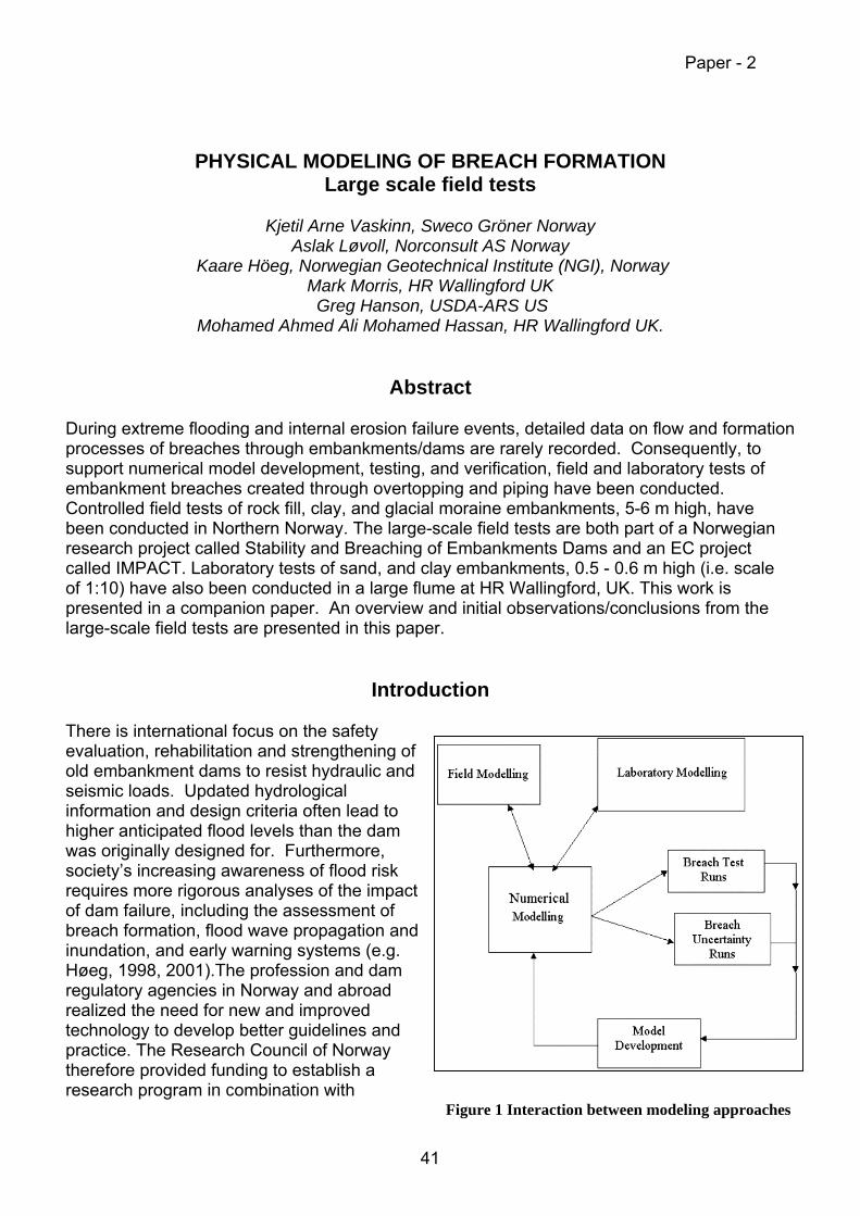
PHYSICAL MODELING OF BREACH FORMATION Large scale field tests

Kjetil Arne Vaskinn, Sweco Gröner Norway

Aslak Løvoll, Norconsult AS Norway Kaare Höeg, Norwegian Geotechnical Institute (NGI), Norway

Mark Morris, HR Wallingford UK Greg Hanson, USDA-ARS US

Mohamed Ahmed Ali Mohamed Hassan, HR Wallingford UK.

Abstract During extreme flooding and internal erosion failure events, detailed data on flow and formation processes of breaches through embankments/dams are rarely recorded. Consequently, to support numerical model development, testing, and verification, field and laboratory tests of embankment breaches created through overtopping and piping have been conducted. Controlled field tests of rock fill, clay, and glacial moraine embankments, 5-6 m high, have been conducted in Northern Norway. The large-scale field tests are both part of a Norwegian research project called Stability and Breaching of Embankments Dams and an EC project called IMPACT. Laboratory tests of sand, and clay embankments, 0.5 - 0.6 m high (i.e. scale of 1:10) have also been conducted in a large flume at HR Wallingford, UK. This work is presented in a companion paper. An overview and initial observations/conclusions from the large-scale field tests are presented in this paper.

Introduction There is international focus on the safety evaluation, rehabilitation and strengthening of old embankment dams to resist hydraulic and seismic loads. Updated hydrological information and design criteria often lead to higher anticipated flood levels than the dam was originally designed for. Furthermore, society’s increasing awareness of flood risk requires more rigorous analyses of the impact of dam failure, including the assessment of breach formation, flood wave propagation and inundation, and early warning systems (e.g. Høeg, 1998, 2001).The profession and dam regulatory agencies in Norway and abroad realized the need for new and improved technology to develop better guidelines and practice. The Research Council of Norway therefore provided funding to establish a research program in combination with

Figure 1 Interaction between modeling approaches

Paper - 2

41

contributions from Norwegian dam owners. The EC and several foreign sponsors also joined the programme. The total budget for the 2001-2004 programme was ca. NOK 19 mill (ca. USD 2.9 mill). In addition to significant financial support, Statkraft SF, Norway’s biggest dam owner, allowed the use of the Rössvatn Dam spillway gates and reservoir to supply water to the field tests located downstream, and also provided other services to the research project.. Furthermore, BC Hydro, Canada has sponsored additional testing related to the use of geophysical methods for the possible detection of internal leakage (erosion) in embankment dams. Initiation of the European IMPACT1 Project was undertaken in parallel with the Norwegian project. An important part of the IMPACT project is the undertaking of field, laboratory and numerical modeling of breach formation through embankments. Objectives for this modeling work are to: • Establish a better understanding of the embankment breaching process • Provide data for numerical model validation, calibration and testing, and hence improve

modeling tool performance • Provide information / data to assess the scaling effect between field and laboratory

experiments • Identify best approach /approaches to simulate breach formation through embankments • Assess and quantify the level of uncertainty of the current breach modeling techniques Figure 1 shows the interaction between the three modeling approaches undertaken within the IMPACT project. In this paper, details of large-scale field modeling are given. Two additional companion papers detail the laboratory modeling, breach data analysis and uncertainty assessment (Hassan et al, 2004 and Morris et al, 2004)

Description of the embankment breach test site

The large scale embankment test site is located in the middle of Norway in Nordland County and the Hemnes Municipality, near the town of Mo i Rana. The location is shown in Figure 2. On the detailed map the Røssvatn Reservoir and Røssåga River flowing north and into Sørfjorden is seen. Figure 3 shows a picture of the test area with the Røssvassdammen Dam and about 1000 m of the Røssåga River. The test site is located as indicated on the picture, about 600 m downstream of the Røssvassdammen Dam. The location downstream of the Røssvassdammen Dam makes it possible to control the inflow to the reservoir behind the test dam by regulating one or more of the three flood gates. Røssvatn is the intake reservoir for Upper Røssåga power plant which outlets into Stormyr-bassenget reservoir at an elevation of 247.9. The 8500 m reach of the 1 IMPACT Project: Investigation of Extreme Flood Processes and Uncertainty. EC Contract No: EVG1-CT-2001-00037. www.impact-project.net

Figure 2 Location of the test-site

Paper - 2

42

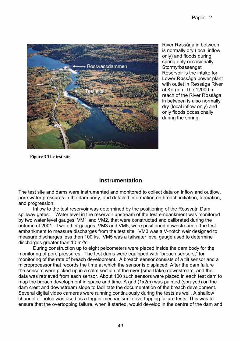
River Røssåga in between is normally dry (local inflow only) and floods during spring only occasionally. Stormyrbassenget Reservoir is the intake for Lower Røssåga power plant with outlet in Røssåga River at Korgen. The 12000 m reach of the River Røssåga in between is also normally dry (local inflow only) and only floods occasionally during the spring.

Instrumentation The test site and dams were instrumented and monitored to collect data on inflow and outflow, pore water pressures in the dam body, and detailed information on breach initiation, formation, and progression. Inflow to the test reservoir was determined by the positioning of the Rossvatn Dam spillway gates. Water level in the reservoir upstream of the test embankment was monitored by two water level gauges, VM1 and VM2, that were constructed and calibrated during the autumn of 2001. Two other gauges, VM3 and VM5, were positioned downstream of the test embankment to measure discharges from the test site. VM3 was a V-notch weir designed to measure discharges less then 100 l/s. VM5 was a tailwater level gauge used to determine discharges greater than 10 m3/s. During construction up to eight peizometers were placed inside the dam body for the monitoring of pore pressures. The test dams were equipped with “breach sensors,” for monitoring of the rate of breach development. A breach sensor consists of a tilt sensor and a microprocessor that records the time at which the sensor is displaced. After the dam failure the sensors were picked up in a calm section of the river (small lake) downstream, and the data was retrieved from each sensor. About 100 such sensors were placed in each test dam to map the breach development in space and time. A grid (1x2m) was painted (sprayed) on the dam crest and downstream slope to facilitate the documentation of the breach development. Several digital video cameras were running continuously during the tests as well. A shallow channel or notch was used as a trigger mechanism in overtopping failure tests. This was to ensure that the overtopping failure, when it started, would develop in the centre of the dam and

Figure 3 The test-site

Paper - 2

43

not towards the abutments. Otherwise the presence of the abutments would interfere with the development of the breach opening both vertically and laterally.

Field Test program A total of 7 field tests (Table 1) have been performed with 5 of these tests as part of the IMPACT project. All the test embankments, with the exception of Test No.4, were tested to complete failure, but the tests were run in stages to gather information for sub-projects a) and b) before failure occurred. Table 1 Listing of field tests. Test No.

Type of dam Objective EC-IMPACT

1 Homogeneous rockfill dam a) three different test with

specially built drainage toe b) Toe removed and the dam

brought to failure

Test of stability with high through flow and breaching mechanism of a rock filling.

2 (1-2002)

Homogeneous clay fill dam Breaching mechanism of a homogenous cohesive dam

IMPACT

3 (2-2002)

Homogenous gravel dam a) With a rockfill berm up the

downstream slope b) With rockfill berm partly

removed c) With rockfill berm removed

and dam brought to failure

Test of stability of gravel dam and study of the breaching mechanism of a dam of non-cohesive material

3C is part of the IMPACT project

4 Homogeneous rockfill dam, but with a smaller crest width and coarser rockfill than that used in Test # 1.

Test of stability with high through flow and breaching mechanism of a rock filling.

5 (1-2003)

Rockfill dam with central moraine core. Dam was failed by overtopping

Study of the breaching mechanism

IMPACT

6 (2-2003)

Rockfill dam with central moraine core. Dam was failed by internal erosion

Study of the breaching mechanism

IMPACT

7 (3-2003)

Homogeneous dam made of same moraine as for the core in Tests # 5 and #6. Dam was failed by internal erosion.

Test #7 was run to compare the progression of the breaching process with that observed in test # 6

IMPACT

Paper - 2

44

Test 1-2002 Homogenous clay dam

Figure 4 Homogenous clay fill dam (from Höeg et al. 2004) The layout of the test dam 1-2002 is shown in Figure 4.The sieve curve for the clay(marine clay) is shown in figure 5. The dam was constructed during the period 14 August to 10 September 2002 to the specifications shown in Figure 4. A 0.5 m deep and 3 m wide channel at the top of the dam was made for initiation of the breach. During construction the soil was placed in 15 centimeter layers and mechanically compacted. Due to high water content in the borrow material (w = 28-33%) and extremely wet weather conditions, construction of the dam was difficult. Therefore, construction procedures were altered, placement layer thickness was increased to 0.4 m and the compaction pressure was reduced. Figure 6 shows 4 pictures taken during the test. The outflow hydrograph is shown in Figure 7.

Figure 5 Sieve curve for clay.

Paper - 2

45

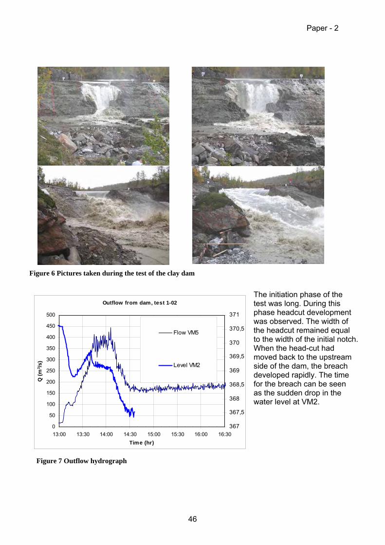
Figure 6 Pictures taken during the test of the clay dam

The initiation phase of the test was long. During this phase headcut development was observed. The width of the headcut remained equal to the width of the initial notch. When the head-cut had moved back to the upstream side of the dam, the breach developed rapidly. The time for the breach can be seen as the sudden drop in the water level at VM2.

Figure 7 Outflow hydrograph

Outflow from dam, test 1-02

0

50

100

150

200

250

300

350

400

450

500

13:00 13:30 14:00 14:30 15:00 15:30 16:00 16:30Time (hr)

Q (m

3 /s)

367

367,5

368

368,5

369

369,5

370

370,5

371

Flow VM5

Level VM2

Paper - 2

46

Test 2-2002 Homogenous gravel dam

Figure 8a Test of homogenous gravel dam. (from Höeg et al. 2004)

The layout of the test dam 2-2002 is shown in Figure 8a. The sieve curve for the gravel used in the dam is shown in Figure 8b. Figure 9 shows 4 pictures taken during the test. The outflow hydrograph is shown in Figure 10.The test was conducted late in the autumn of 2002. The air temperature was zero degree Celsius (freezing point) the night before the test. The upper

layer of the dam (a few centimeters) was frozen. Before we could start the test we had to melt that layer. There was no release of water from the gates at Røssvassdammen during the test. Consequently the level of the test dam was lowered rapidly during failure.

The initial phase of the failure process was not as expected. The overtopping discharge was steadily increased from 30 to 50 l/s in a 2-meter wide notch for 45 minutes. During this phase there was headcut development more or less the same way as in the clay dam. Following the breach initiation the vertical erosion finished after 5 minutes and the horizontal erosion after 5-10 minutes

Sieve curves at every layer dam 2-02 (sandy

0.074 0.149 0.297 0.59 1.19 2.38 4.76 9.52 19.05 38.1 76.2

0 10 20 30 40 50 60 70 80 90

100

0.01 0.1 1 10 100d [mm]

% finer

than

d

U.S. Standard Sieves (mm) 1 1.5 2 2.5 3 3.5 4

Figure 8b Sieve curves for test 2-2002

Paper - 2

47

Figure 9 Pictures taken during the test of the gravel dam

Outflow from dam: Test 2C-02

0

20

40

60

80

100

120

140

12:00 12:30 13:00 13:30 14:00 14:30

Time (hh:mm)

Q (m

3 /s)

Figure 10 Reservoir level and outflow hydrograph during the gravel dam test

Paper - 2

48

Test 1-2003 Rockfill dam with central moraine core The layout of the test dam 1-2003 is shown in Figure 11. The dam consists of a moraine core supported by rockfill on the upstream and downstream sides. The grading curves for the moraine (1) and rockfill on the downstream side (2) are shown in Figure 12. On the upstream side the rock material (3) was 300 - 400 mm.

Figure 11 Composite dam: Rockfill with moraine core. (from Höeg et al. 2004)

Grain distribution moraine and rockfill dam 1-03 0,074 0,149 0,297 0,59 1,19 2,38 4,76 9,52 19,05 38,1 76,2 152,4 406,4

0

10

20

30

40

50

60

70

80

90

100

0,001 0,01 0,1 1 10 100 1000d (mm)

Rel

ativ

e w

eigh

t of g

rain

s <

d in

%

U.S. Standard Sieves (mm)MoraineMoraine < 19 mmRockfill

Figure 12 Sieve curves for the materials in the composite dam

Paper - 2

49

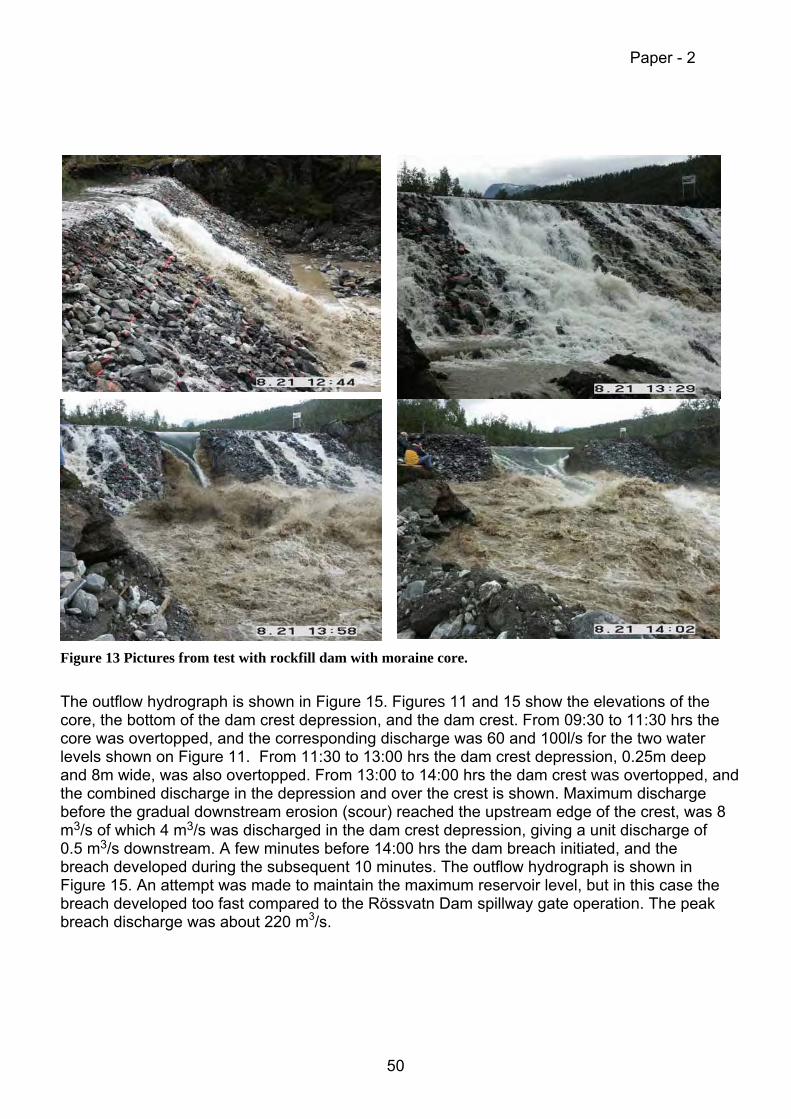
Figure 13 Pictures from test with rockfill dam with moraine core. The outflow hydrograph is shown in Figure 15. Figures 11 and 15 show the elevations of the core, the bottom of the dam crest depression, and the dam crest. From 09:30 to 11:30 hrs the core was overtopped, and the corresponding discharge was 60 and 100l/s for the two water levels shown on Figure 11. From 11:30 to 13:00 hrs the dam crest depression, 0.25m deep and 8m wide, was also overtopped. From 13:00 to 14:00 hrs the dam crest was overtopped, and the combined discharge in the depression and over the crest is shown. Maximum discharge before the gradual downstream erosion (scour) reached the upstream edge of the crest, was 8 m3/s of which 4 m3/s was discharged in the dam crest depression, giving a unit discharge of 0.5 m3/s downstream. A few minutes before 14:00 hrs the dam breach initiated, and the breach developed during the subsequent 10 minutes. The outflow hydrograph is shown in Figure 15. An attempt was made to maintain the maximum reservoir level, but in this case the breach developed too fast compared to the Rössvatn Dam spillway gate operation. The peak breach discharge was about 220 m3/s.

Paper - 2

50

VM2 and overtopping discharge

370,0

370,1

370,2

370,3

370,4

370,5

370,6

370,7

370,8

370,9

371,0

21.08 08:30 21.08 09:30 21.08 10:30 21.08 11:30 21.08 12:30 21.08 13:30 21.08 14:30

Time

Stag

e (m

asl)

0

1

2

3

4

5

6

7

8

9

10

Dis

char

ge (m

3/s)

level Top core

Dam crest overtopping

Figure 14 Water elevation in the testdam prior to the test

VM5 discharge

0

50

100

150

200

250

21.08 11 21.08 12 21.08 13 21.08 14 21.08 15

Time (dd.mm hh)

Dis

char

ge (m

3 /s)

Figure 15 Outflow hydrograph from the test with rockfill dam

Paper - 2

51

Test 2-2003 Rockfill dam with central moraine core breaching by piping The layout of the test dam 2-2003 is shown in Figure 16. This dam was made of the same material, as the dam in test 1-2003. Two different trigger mechanisms to initiate internal erosion were built into the dam. Two pipes, diameter of 200 mm, with openings on the top were used, as triggers (Figure 17). These pipes were covered with homogenous sand. Trigger device number one was covered with a sand layer of 1 by 1 meter. The sand layer around trigger number 2 was extended to the top of the dam. At the start of the test the pipes were closed at the downstream end. By opening of the valve at the downstream end of the devices the sand was flushed out and the internal erosion started. Trigger device number one was opened first and was kept open for 4 days, but we had no failure of the dam. After opening trigger device number 2 a sinkhole rapidly formed on top of the dam. This can be seen in Figure 18. The sinkhole formed a notch through the dam and the dam failed the same way as by overtopping. The outflow hydrograph is shown in Figure 19.

Figure 16 Composite dam with moraine core breaching by overtopping. (from Höeg et al. 2004)

Figure 17 Construction of trigger devices

Paper - 2

52

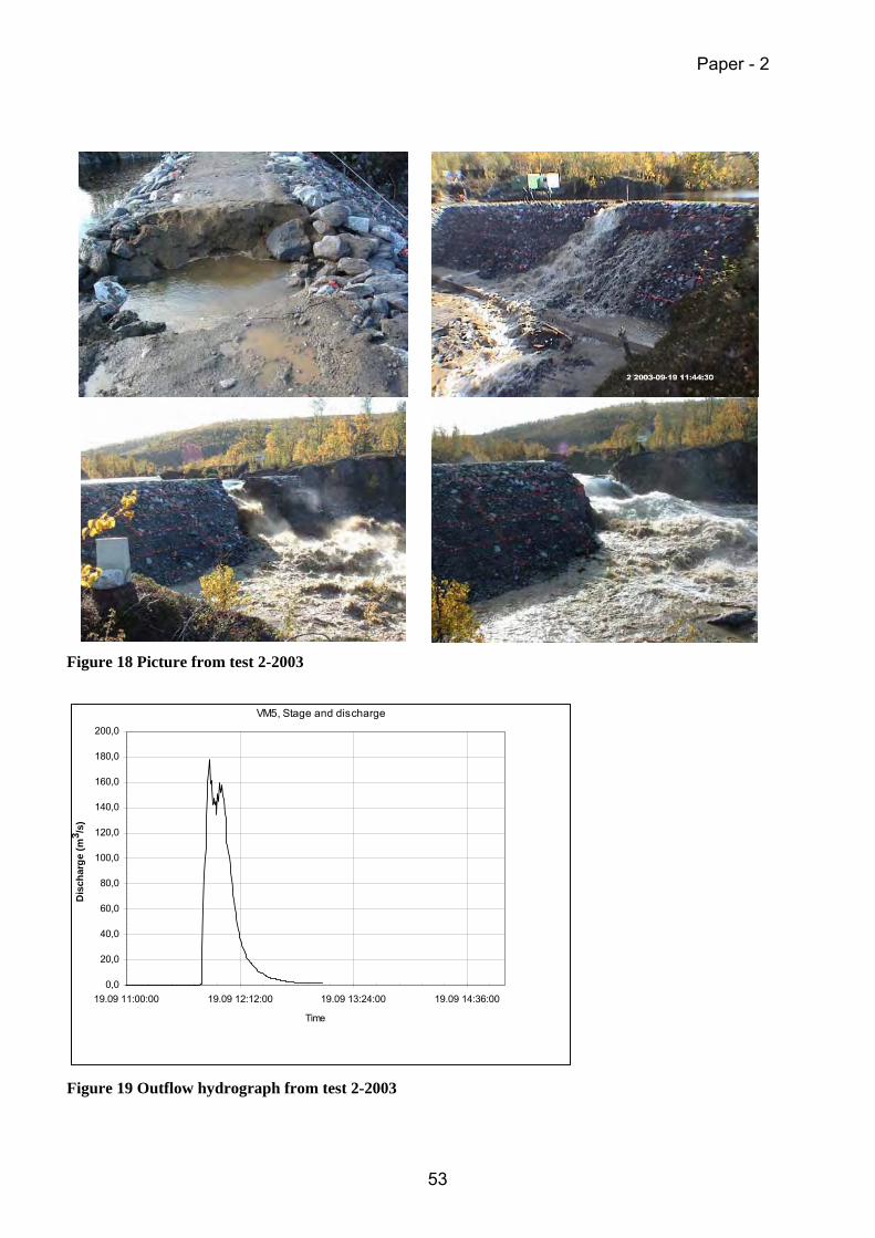
Figure 18 Picture from test 2-2003

VM5, Stage and discharge

0,0

20,0

40,0

60,0

80,0

100,0

120,0

140,0

160,0

180,0

200,0

19.09 11:00:00 19.09 12:12:00 19.09 13:24:00 19.09 14:36:00

Time

Dis

char

ge (m

3 /s)

Figure 19 Outflow hydrograph from test 2-2003

Paper - 2

53

Test 3-2003 Homogenous moraine dam

Test 3-2003 was run to compare the progression of the breaching process with that observed in 2-2003 where the moraine was protected by the rockfill upstream and downstream. The layout of the test dam is shown in Figure 20

Figure 20 Homogenous clay fill dam. (from Höeg et al. 2004) The sieve curve for the moraine is the same as the sieve curve shown in Figure 12. The trigger mechanism was exactly like the trigger mechanism 1 in test 2-2003. Figure 22 shows 4 pictures taken during the test. The failure of this test was very rapid. It took only about 20 minutes from opening of the trigger mechanism until the dam was breached. The outflow hydrograph is shown in Figure 21. It is interesting to note that the piping failure tests 2-2003 and 3-2003 resulted in virtually identical peak discharges.

Figure 21 Outflow hydrograph in test 3-2003

0

20

40

60

80

100

120

140

160

180

200

08.1013:00:03

08.1013:14:27

08.1013:28:51

08.1013:43:15

08.1013:57:39

08.1014:12:03

08.1014:26:27

08.1014:40:51

08.1014:55:15

Time

Dis

char

ge (m

3 /s)

Paper - 2

54

Figure 22 Pictures taken during the test

Conclusions This paper has provided an introduction to field work undertaken in Norway during the last few years, aimed at collecting reliable information and data sets detailing the failure mechanisms of a range of different embankment dams. Reliable data sets now exist for the failure of a range of different large-scale embankment geometries and material types. Analysis of this data has started and is likely to continue for some years. The data will assist in the development of understanding and validation of predictive models. Prior to this analysis, some initial, broad observations may be made based upon field observations and data analysis to date. These include the following: • The data collected for each test comprises a mixture of flows, levels, breach growth

dimensions, video and still photo footage. The failure processes of the different embankments may be observed. Features such as cracking, arching (pipe formation), headcut formation and progression were all observed. Existing breach models does not accurately simulate many of these features.

• The first phase in the external erosion of the downstream slope due to overtopping is slow and very gradual. However, when the scour and unraveling finally reaches the upstream edge of the dam crest, the breaching is rapid and dramatic. The same general observations were made for the rockfill, gravel and clay dams. The opening of the breach first progresses

Paper - 2

55

down to base of the dam, before it expands laterally. The sides of the breach were very steep, almost vertical, in all three materials.

• The rate of breach growth for the homogeneous clay and gravel dams was not as expected. The clay dam failure more quickly, whilst the gravel dam more slowly than expected. It is likely that this was due to the condition of material and nature of construction / compaction. This demonstrates the significant impact that material condition and construction method may have on breach formation and hence the need to consider these aspects within predictive models.

• The internal erosion process, initiated at the defects built into the moraine core of the rockfill dam (Test 2-2003), took a very long time to develop, even in this dam with no filters between the moraine core and the downstream rockfill. Breaching of the dam did not take place until the erosion had proceeded up to the dam crest, and then the dam failed by overtopping as in Test 1-2003, but the breach opening was not so wide.

• The difference in rate of embankment failure for the homogeneous moraine embankment and the composite moraine / rockfill embankment was significant. This demonstrates the importance of the interaction between layers of material within a composite structure. This has implications for overall dam stability and in the development of predictive breach models.

• Many of the field test scenarios simulated typical rockfill embankment dams. As such, there was surprise that the rate and mechanisms of failure observed were typically more resistant than existing analyses and guidelines prescribe.

References

1. Höeg, K. (1998) New dam safety legislation and the use of risk analysis, The International

Journal of Hydropower and Dams, Vol 5, Issue 5, pp 85-89. 2. Höeg, K. (2001) Embankment-dam engineering, safety evaluation and upgrading, Invited

Perspective Lecture, 15th ICSMGE, Vol. 4, pp. 2491-3504, Istanbul, Turkey. 3. Höeg, K., Løvoll, A. and Vaskinn, K. A (2004) Stability and breaching of embankment

dams: field tests on 6 meter high dams. The International Journal of Hydropower and Dams, Issue 5, 2004.

4. Hassan MAA, Morris MW, Hanson G and Lakhal K (2004). Breach formation: Laboratory and numerical modelling of breach formation. Association of State Dam Safety Officials: Dam Safety 2004. Phoenix, Arizona Sept 2004.

5. Morris MW, Hassan MAA, Alcrudo F, Zech Y and Lakhal K (2004). Process uncertainty: assessing and combining uncertainty between models. Association of State Dam Safety Officials: Dam Safety 2004. Phoenix, Arizona Sept 2004.

Acknowledgements The authors wish to thank the IMPACT project partners and the partners of the Norwegian project for their valuable help. The project was made possible through funding from the following institutions: The Research Council of Norway (NFR) Norwegian Electricity Industry Association (EBL-K), several Norwegian dam owners, the Norwegian Water Resources and Energy Directorate (NVE), the EC-Impact Project (European Commission), Swedish Electrical Utilities (ELFORSK), Sweden, Hydro Québec, Canada and Electricité de France (EDF), France

Paper - 2

56

BREACH FORMATION: Laboratory and Numerical Modelling of Breach Formation

Mohamed Hassan, HR Wallingford UK

Mark Morris, HR Wallingford UK Greg Hanson, USDA-ARS US

Karim Lakhal, Engineering School of Science and Technology of Lyon France

Abstract

Our ability to predict the flow and rate of development of a breach through a flood embankment or dam to date has been limited. Lack of data and understanding of the breach processes are probably the main reasons for this. A program of field and laboratory experiments has been undertaken under the IMPACT project to improve the understanding of the breach processes. In conjunction with this, a programme of numerical modelling comparison and development has been conducted using the data from field and laboratory experiment undertaken under the project. This paper presents details of the undertaken laboratory experiments and numerical modelling. Details of the field experiments are given in a companion paper.

Introduction

An important part of the IMPACT1project is the undertaking of field, laboratory and numerical modelling of breach formation through embankments. Objectives for this modelling work are to: • Establish a better understanding of the

embankment breaching process • Provide data for numerical model

validation, calibration and testing, and hence improve modelling tools performance

• Provide information / data to assess the scaling effect between field and laboratory experiments

• Identify best approach /approaches to simulate breach formation through embankments

• Assess and quantify the level of uncertainty of the current breach modelling techniques

Figure 1 shows the interaction between the three modelling approaches undertaken under the IMPACT project. In this paper, details of the laboratory modelling, the breach test

1 For details on the IMPACT project visit www.impact-project.net

Figure 1: Interaction between modelling approaches

Paper - 3

57

runs, and part of the numerical modelling are given. In another two companion papers2 details of the field modelling and breach uncertainty runs are given.

Laboratory Modelling

A total of 22 laboratory experiments have been undertaken at HR Wallingford in the UK.

The overall objective of these tests was to better understand the breach processes in embankments failed by overtopping or piping and identify the important parameters that influence these processes. These tests were divided into 3 series. Table 1 shows the details of each series of tests. The focus, in this paper, is on the analysis of series #1 and #2.

Table 1: Laboratory tests description

Laboratory Test Description Laboratory Test Objective

Series # 1 (9 tests)

This series of tests was based around the homogeneous non-cohesive field test at scale of 1:10. Each embankment was built from non-cohesive material, however, more than one grading of sediment were used along with different embankment geometry, breach location and time before failure (seepage effect).

To better understand breach formation processes and to identify the effect of a variety of parameters on these processes in homogeneous non-cohesive embankments failed by overtopping

Series # 2 (8 tests)

This series of tests was based around the homogeneous cohesive field test at scale of 1:10. Each embankment was built from cohesive material, however, two different grading of sediment were used along with different embankment geometry, compaction effort and moisture content.

To better understand breach formation processes and to identify the effect of a variety of parameters on these processes in homogeneous cohesive embankments failed by overtopping

Assess initiation of the piping mechanism and dimensions for the homogeneous field test

Provide information about the pipe formation to assist in development of the field test failure mechanism

Series # 3 (5 tests)

Material brought from a UK flood embankment. Samples were 1m (W) x 1m (L) x 0.8m (D)

Monitor piping initiation and development

Series #1 - breach processes

The following processes were observed during the breach formation for this series of tests:

1. Water erodes the downstream slope and the slope becomes milder. Head cutting was not observed in this series of tests

2. The crest of the embankment retreats and erodes downward 3. Once the breach is fully developed (i.e. material is nearly eroded to the base), the material

below the water level is eroded. This undermines the slopes and leads to block failure 4. The above processes continue until there is not enough water to erode more material 5. Upstream slope erosion was also observed leading to a curved ‘bell mouth’ entrance to the

breach. This ‘bell mouth’ weir controlled flow through the breach. Slumping was also 2 See special workshop #1: “International Progress in Dam Breach Evaluation”

Paper - 3

58

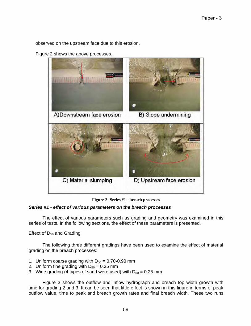
observed on the upstream face due to this erosion.

Figure 2 shows the above processes.

Figure 2: Series #1 - breach processes

Series #1 - effect of various parameters on the breach processes The effect of various parameters such as grading and geometry was examined in this

series of tests. In the following sections, the effect of these parameters is presented.

Effect of D50 and Grading The following three different gradings have been used to examine the effect of material

grading on the breach processes: 1. Uniform coarse grading with D50 = 0.70-0.90 mm 2. Uniform fine grading with D50 = 0.25 mm 3. Wide grading (4 types of sand were used) with D50 = 0.25 mm

Figure 3 shows the outflow and inflow hydrograph and breach top width growth with

time for grading 2 and 3. It can be seen that little effect is shown in this figure in terms of peak outflow value, time to peak and breach growth rates and final breach width. These two runs

Paper - 3

59

show that the effect of grading is insignificant at this laboratory scale.

-0.1

0

0.1

0.2

0.3

0.4

0.5

0.6

0.7

0.8

0.9

2700 2800 2900 3000 3100 3200 3300 3400 3500

Time (sec)

Dis

char

ge

(m3 /s

)

-0.5

0

0.5

1

1.5

2

2.5

3

3.5

4

4.5

Wid

th (

m)

Outflow Wide Grading

Inflow Wide Grading

Outflow Uniform FineGrading

Inflow Uniform Fine Grading

Breach Top Width UniformFine Grading

Breach Top Width WideGrading

Figure 33: Grading variation results

Effect of Breach Location To examine the effect of the breach location, the initial breach notch was placed once

on the centre and once on the side of two different embankments with similar properties and same geometry. Figure 4 shows the outflow and inflow hydrograph and breach top width growth with time for these two tests.

-0.1

0

0.1

0.2

0.3

0.4

0.5

0.6

0.7

0.8

2700 2800 2900 3000 3100 3200 3300 3400 3500

Time (sec)

Dis

char

ge

(m3 /s

)

-0.5

0

0.5

1

1.5

2

2.5

3

3.5

4

Wid

th (

m)

Outflow Side Breach

Inflow Side Breach

Outflow Central Breach

Inflow Central Breach

Side Breach Top Width

Central Breach TopWidth

Figure 4: Breach location variation results

It is noticeable that a side breach has a lower peak outflow, erosion rate and final breach width. These two runs show that the effect of breach location is significant at this laboratory scale.

3 The authors acknowledge that it is difficult to interpret the figures unless they are in colour. If this not the case, the reader can obtain a digital coloured copy from www.impact-project.net or the conference CD.

Paper - 3

60

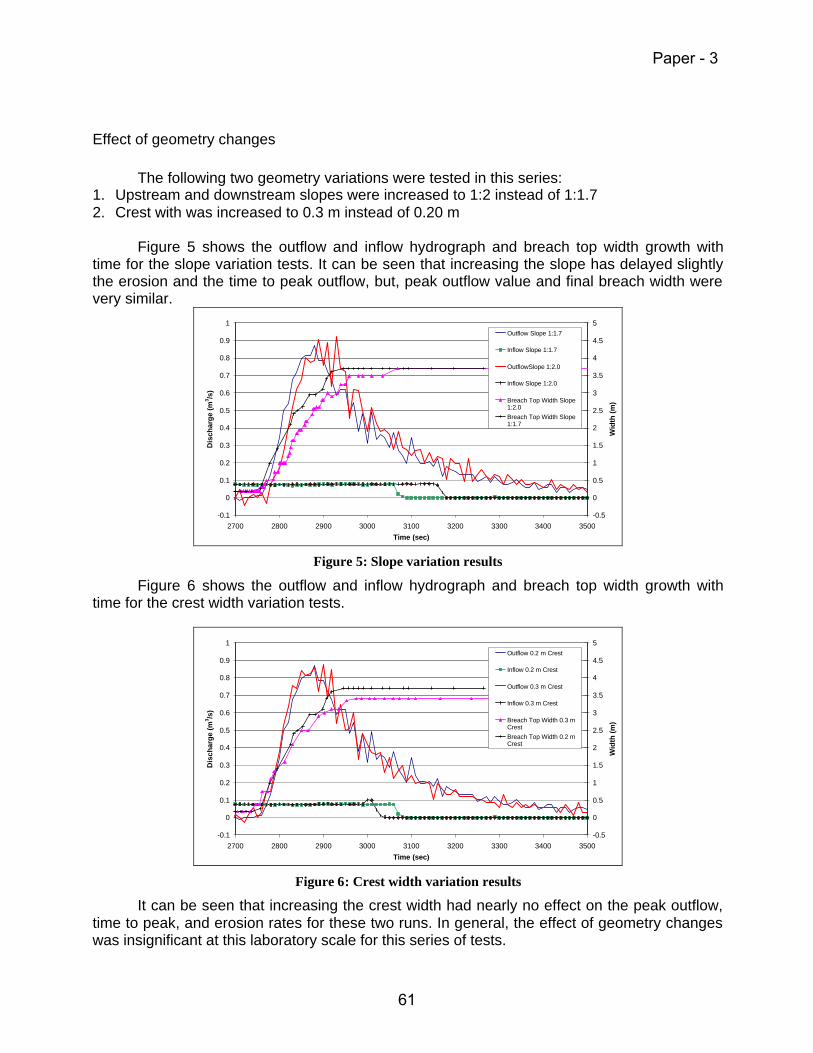
Effect of geometry changes The following two geometry variations were tested in this series:

1. Upstream and downstream slopes were increased to 1:2 instead of 1:1.7 2. Crest with was increased to 0.3 m instead of 0.20 m

Figure 5 shows the outflow and inflow hydrograph and breach top width growth with time for the slope variation tests. It can be seen that increasing the slope has delayed slightly the erosion and the time to peak outflow, but, peak outflow value and final breach width were very similar.

-0.1

0

0.1

0.2

0.3

0.4

0.5

0.6

0.7

0.8

0.9

1

2700 2800 2900 3000 3100 3200 3300 3400 3500

Time (sec)

Dis

char

ge

(m3 /s

)

-0.5

0

0.5

1

1.5

2

2.5

3

3.5

4

4.5

5

Wid

th (

m)

Outflow Slope 1:1.7

Inflow Slope 1:1.7

OutflowSlope 1:2.0

Inflow Slope 1:2.0

Breach Top Width Slope1:2.0

Breach Top Width Slope1:1.7

Figure 5: Slope variation results

Figure 6 shows the outflow and inflow hydrograph and breach top width growth with time for the crest width variation tests.

-0.1

0

0.1

0.2

0.3

0.4

0.5

0.6

0.7

0.8

0.9

1

2700 2800 2900 3000 3100 3200 3300 3400 3500

Time (sec)

Dis

char

ge

(m3 /s

)

-0.5

0

0.5

1

1.5

2

2.5

3

3.5

4

4.5

5

Wid

th (

m)

Outflow 0.2 m Crest

Inflow 0.2 m Crest

Outflow 0.3 m Crest

Inflow 0.3 m Crest

Breach Top Width 0.3 mCrest

Breach Top Width 0.2 mCrest

Figure 6: Crest width variation results

It can be seen that increasing the crest width had nearly no effect on the peak outflow, time to peak, and erosion rates for these two runs. In general, the effect of geometry changes was insignificant at this laboratory scale for this series of tests.

Paper - 3

61

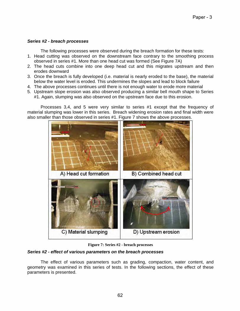
Series #2 - breach processes

The following processes were observed during the breach formation for these tests: 1. Head cutting was observed on the downstream face contrary to the smoothing process

observed in series #1. More than one head cut was formed (See Figure 7A) 2. The head cuts combine into one deep head cut and this migrates upstream and then

erodes downward 3. Once the breach is fully developed (i.e. material is nearly eroded to the base), the material

below the water level is eroded. This undermines the slopes and lead to block failure 4. The above processes continues until there is not enough water to erode more material 5. Upstream slope erosion was also observed producing a similar bell mouth shape to Series

#1. Again, slumping was also observed on the upstream face due to this erosion.

Processes 3,4, and 5 were very similar to series #1 except that the frequency of material slumping was lower in this series. Breach widening erosion rates and final width were also smaller than those observed in series #1. Figure 7 shows the above processes.

Figure 7: Series #2 - breach processes

Series #2 - effect of various parameters on the breach processes The effect of various parameters such as grading, compaction, water content, and

geometry was examined in this series of tests. In the following sections, the effect of these parameters is presented.

Paper - 3

62

Effect of material type and grading The following two material grades were used to examine the effect of material type and

grading on the breach processes: 1. Fine-grained clay material with D50 = 0.005 mm with 24-43 % of clay (This was used for

all the tests except one where the moraine material was used) 2. Moraine material with D50 = 0.715 mm with less than 10 % fines.

Figure 8 shows the outflow and inflow hydrograph and breach top width growth with time for the material variation tests. It is quite clear that the moraine material was more erodible than the clay material. This has accelerated the erosion process and led to a higher peak outflow and larger final breach width.

-0.100

0.000

0.100

0.200

0.300

0.400

0.500

0.600

0.700

0 1000 2000 3000 4000 5000 6000 7000 8000

Time (sec)

Dis

char

ge

(m^3

/s)

0

0.5

1

1.5

2

2.5

3

3.5

4

Wid

th (

m)

Outflow clay

Inflow clay

Outflow moraine

Inflow moraine

Breach Top Width clay

Breach Top Width moraine

Figure 8: Material variation results

Effect of compaction Two compaction efforts were used, to examine the effect of compaction on the clay

material, with one compaction effort half of the other. Figure 9 shows the outflow and inflow hydrograph and breach top width growth with time for the compaction variation tests. Halving the compaction had an impact on the breaching processes for these two test cases but that impact is clouded by the effects of the compaction water content which is discussed in the next section. The decrease in compaction effort has accelerated the erosion process and led to a higher peak outflow and final breach width at this laboratory scale. The compaction water content for the higher compaction effort case was 25% and the half compaction effort case was 22%. This decrease in water content, as discussed in the next section, also accelerates erosion rates.

Paper - 3

63

-0.1

0

0.1

0.2

0.3

0.4

0.5

0.6

0 1000 2000 3000 4000 5000 6000 7000 8000

Time (sec)

Dis

char

ge

(m^3

/s)

0

0.5

1

1.5

2

2.5

3

3.5

Wid

th (

m)

Outflow normal compaction

Inflow normal compaction

Outflow half compaction

Inflow half compaction

Breach Top Width normal compaction

Breach Top Width half compaction

Figure 9: Compaction variation results

Effect of water content To check the effect of the compaction water content, two different values of water

content were used. The first was very near to the optimum water content (30 %) for the material used in this series of tests. The other was the natural water content of this material (24 %) which is lower than the optimum water content value.

-0.050

0.000

0.050

0.100

0.150

0.200

0.250

0.300

0.350

0 2000 4000 6000 8000 10000 12000 14000

Time (sec)

Dis

char

ge

(m^3

/s)

0

0.25

0.5

0.75

1

1.25

1.5

1.75

2

Wid

th (

m)

Outflow low water content

Inflow low water content

Outflow optimum water content

Inflow optimum water content

Breach Top Width low water content

Breach Top Width optimum water content

Figure 10: Water content variation results

The compaction effort for these two tests was basically the same therefore, the effect on erosion and outflow can be attributed to changes in the compaction water content. Figure 10 shows the outflow and inflow hydrograph and breach top width growth with time for the water content variation tests. Changing the water content to the optimum has significantly change the

Paper - 3

64

erosion properties of the material used. The embankment with optimum water content resisted failure and at the end of the test only partially failed with a smaller breach width and a lower peak outflow value compared to the other embankment. Laboratory tests, undertaken using the Jet-Test apparatus (ASTM, 1996), showed a difference in the erodibility of about 93 % between the two embankments.

Effect of geometry changes The following two geometry variations were tested in this series:

1. Downstream slope was changed to 1V:1H instead of 1V:2H 2. Downstream slope was changed to 1V:3H instead of 1V:2H

Figure 11 shows the outflow and inflow hydrograph and breach top width growth with time for the slope variation No. 1. Both tests, the test with 1V:1H and the test with 1V:3H slopes, sped up failure and led to a higher peak outflow. This was not expected for the 1V:3H slope embankment as it had more material that the other two slopes (i.e. longer failure time). This could be due to the fact that both tests were at a lower bulk density than the 1V:2H slope and also at lower water content. These issues clouded the outcome of both tests and made the results of these two tests inconclusive.

-0.050

0.000

0.050

0.100

0.150

0.200

0.250

0.300

0.350

0.400

0 1000 2000 3000 4000 5000 6000 7000 8000Time (sec)

Dis

char

ge

(m^3

/s)

0

0.25

0.5

0.75

1

1.25

1.5

1.75

2

2.25

Wid

th (

m)Outflow 1:2 slope

Inflow1:2 slope

Outflow 1:1 slope

Inflow 1:1 slope

Breach Top Width 1:2 slope

Breach Top Width 1:1 slope

Figure 11: Geometry variation results

Numerical Modelling - Breach Test Runs

Extensive numerical modelling has been undertaken by selected members of the IMPACT project team and the value of model comparison was enhanced by additional participation from modellers world-wide (See Table 2 for details). A significant number of numerical model runs has been undertaken as blind tests to ensure complete objectivity. Blind means that numerical modellers were asked to undertake their work and submit their results before the results from the field and laboratory tests are released. Modellers were then invited to submit further (revised) modelling results after receiving the field or lab test results (Aware testing). Results presented in this paper are blind except for laboratory series #1 where only aware testing was undertaken due to data processing errors.

Paper - 3

65

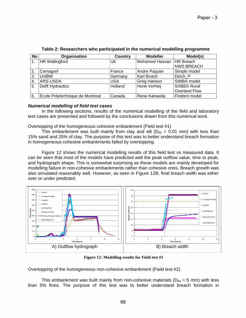
Table 2: Researchers who participated in the numerical modelling programme

No Organisation Country Modeller Model(s) 1. HR Wallingford UK Mohamed Hassan HR Breach

NWS BREACH 2. Cemagref France Andre Paquier Simple model 3. UniBW Germany Karl Broich Deich_P 4. ARS-USDA USA Greg Hanson SIMBA model 5. Delft Hydraulics Holland Henk Verheij SOBEK Rural

Overland Flow 6. Ecole Polytechnique de Montreal Canada Rene Kahawita Firebird model

Numerical modelling of field test cases

In the following sections, results of the numerical modelling of the field and laboratory test cases are presented and followed by the conclusions drawn from this numerical work. Overtopping of the homogeneous cohesive embankment (Field test #1)

This embankment was built mainly from clay and silt (D50 = 0.01 mm) with less than 15% sand and 25% of clay. The purpose of this test was to better understand breach formation in homogeneous cohesive embankments failed by overtopping.

Figure 12 shows the numerical modelling results of this field test vs measured data. It

can be seen that most of the models have predicted well the peak outflow value, time to peak, and hydrograph shape. This is somewhat surprising as these models are mainly developed for modelling failure in non-cohesive embankments rather than cohesive ones. Breach growth was also simulated reasonably well. However, as seen in Figure 12B, final breach width was either over or under predicted.

0

50

100

150

200

250

300

350

400

450

0 2 4 6 8 10 12

Time (hours)

Flo

w (

m3 /s

)

DEICH

Cemagref Model

FireBird

SOBEK

HR BREACH

Measured Data

Moving Average Outflow

NWS BREACH

A) Outflow hydrograph

0

5

10

15

20

25

30

35

40

0 2 4 6 8 10 12Time (hours)

Bre

ach

wid

th (

m)

DEICH

Cemagref Model

SOBEK

HR BREACH

Measured Data

NWS BREACH

B) Breach width

Figure 12: Modelling results for Field test #1

Overtopping of the homogeneous non-cohesive embankment (Field test #2)

This embankment was built mainly from non-cohesive materials (D50 ≈ 5 mm) with less

than 5% fines. The purpose of this test was to better understand breach formation in

Paper - 3

66

homogeneous non-cohesive embankments failed by overtopping.

0

20

40

60

80

100

120

140

0 1000 2000 3000 4000 5000 6000 7000 8000 9000 10000

Time (s)

Ou

tflo

w (

m3/

s)

DEICH

CemagrefModelSOBEK

MeasuredDataHR BREACH

NWSBREACH

A) Outflow hydrograph

0

2

4

6

8

10

12

14

16

0 1000 2000 3000 4000 5000 6000 7000 8000 9000 10000

Time (s)

Ou

tflo

w (

m3/

s)

DEICH Cemagref Model SOBEK HR BREACH NWS BREACH

B) Breach width

Figure 13: Modelling results for Field test #2

Figure 13 shows the numerical modelling results of this field test vs measured data (If available). It is quite clear that all of the models have underestimated the time to peak (See Figure 13A). Investigation of this issue revealed that the test conditions given to modellers were different, in terms of the initiation of the breach, from those actually occurred in the field. This resulted in underestimation of the time to peak. Despite that, results of the peak outflow still represent what would be the output of the model if field test conditions were used. It can be noted from Figure 13A that the scatter of the results is wider than that of Field test #1. This is again surprising as these models are mainly developed for modelling failure in non-cohesive embankments. Models have either over or under predicted the final breach width of the breach compared with the average final measured breach width that was about 12 m. Overtopping of homogeneous composite embankment (Field test #3)

The upstream and downstream shoulders of this embankment were built from rock fill with a central moraine core. The purpose of this test was to better understand breach formation in composite embankments failed by overtopping

Figure 14 shows the numerical modelling results of this field test vs measured data (If available). It can be seen that most of the models have predicted well the peak outflow value, time to peak, and to a certain extent the hydrograph shape. This was unexpected, as most the models used to model this case do not model the complex processes due to the existence of the central core. This poses an important question of how simple could we make models without being far from predicting what really happens. Models have either over or under predicted the final breach width of the breach compared with the final measured width that was about 18 m.

Paper - 3

67

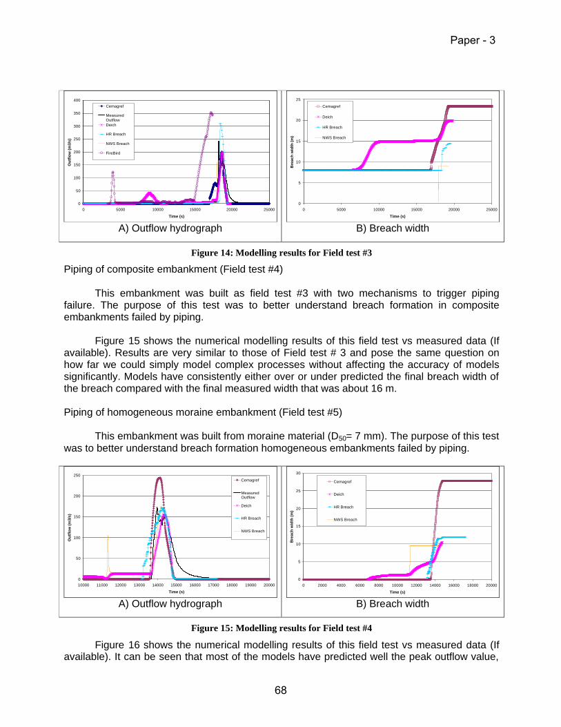
0

50

100

150

200

250

300

350

400

0 5000 10000 15000 20000 25000

Time (s)

Ou

tflo

w (

m3/

s)

Cemagref

MeasuredOutflowDeich

HR Breach

NWS Breach

FireBird

A) Outflow hydrograph

0

5

10

15

20

25

0 5000 10000 15000 20000 25000

Time (s)

Bre

ach

wid

th (

m)

Cemagref

Deich

HR Breach

NWS Breach

B) Breach width

Figure 14: Modelling results for Field test #3

Piping of composite embankment (Field test #4)

This embankment was built as field test #3 with two mechanisms to trigger piping failure. The purpose of this test was to better understand breach formation in composite embankments failed by piping.

Figure 15 shows the numerical modelling results of this field test vs measured data (If available). Results are very similar to those of Field test # 3 and pose the same question on how far we could simply model complex processes without affecting the accuracy of models significantly. Models have consistently either over or under predicted the final breach width of the breach compared with the final measured width that was about 16 m.

Piping of homogeneous moraine embankment (Field test #5)

This embankment was built from moraine material (D50= 7 mm). The purpose of this test was to better understand breach formation homogeneous embankments failed by piping.

0

50

100

150

200

250

10000 11000 12000 13000 14000 15000 16000 17000 18000 19000 20000

Time (s)

Ou

tflo

w (

m3/

s)

Cemagref

MeasuredOutflow

Deich

HR Breach

NWS Breach

A) Outflow hydrograph

0

5

10

15

20

25

30

0 2000 4000 6000 8000 10000 12000 14000 16000 18000 20000

Time (s)

Bre

ach

wid

th (

m)

Cemagref

Deich

HR Breach

NWS Breach

B) Breach width

Figure 15: Modelling results for Field test #4

Figure 16 shows the numerical modelling results of this field test vs measured data (If available). It can be seen that most of the models have predicted well the peak outflow value,

Paper - 3

68

time to peak, and the hydrograph shape. Despite that breach growth and breach final width scatter is wide (See Figure 16B) and final breach width was either over or under predicted compared with the final measured width that was about 15 m.

0

20

40

60

80

100

120

140

160

180

200

10000 15000 20000

Time (s)

Ou

tflo

w (

m3/

s)

Cemagref

Measured Outflow

Deich

HR Breach

NWS Breach

A) Outflow hydrograph

0

5

10

15

20

25

30

35

40

0 2000 4000 6000 8000 10000 12000 14000 16000 18000 20000

Time (s)

Bre

ach

wid

th (

m)

Cemagref

Deich

HR Breach

NWS Breach

B) Breach width

Figure 16: Modelling results for Field test #5

Numerical modelling of laboratory test cases Replication of Field test #2 – Laboratory Series #1

This test case was a direct replication of Field test # 2. Geometry and material size was

scaled down to 1:10 scale. Figure 17 shows the numerical modelling results of this test vs measured data. It can be seen that most of the models have predicted well the peak outflow value, time to peak, and the hydrograph shape. Breach growth rate and final breach width were also reasonably predicted by most models in this case, contrary to the rest of the test cases.

0.000

0.200

0.400

0.600

0.800

1.000

1.200

0 1000 2000 3000 4000 5000

Time (s)

Flo

w (

m^3

/s)

MeasuredOutflow

Cemagref

Deich

NWS Breach

Henk

HR Breach

A) Outflow hydrograph

0

1

2

3

4

5

6

7

0 1000 2000 3000 4000 5000

Time (s)

Bre

ach

wid

th (

m)

Cemagref

Measured top width

Deich

Measured bottomwidthSOBEK

NWS Breach

HR Breach

B) Breach width

Figure 17: Modelling results of replication of Field test #2 - Laboratory Series #1

Replication of Field Test #1- Series #2

This test case was a direct replication of Field test # 1. Geometry was scaled down to 1:10 scale. Material was scaled down based on the erodibility rather than geometrically (i.e.

Paper - 3

69

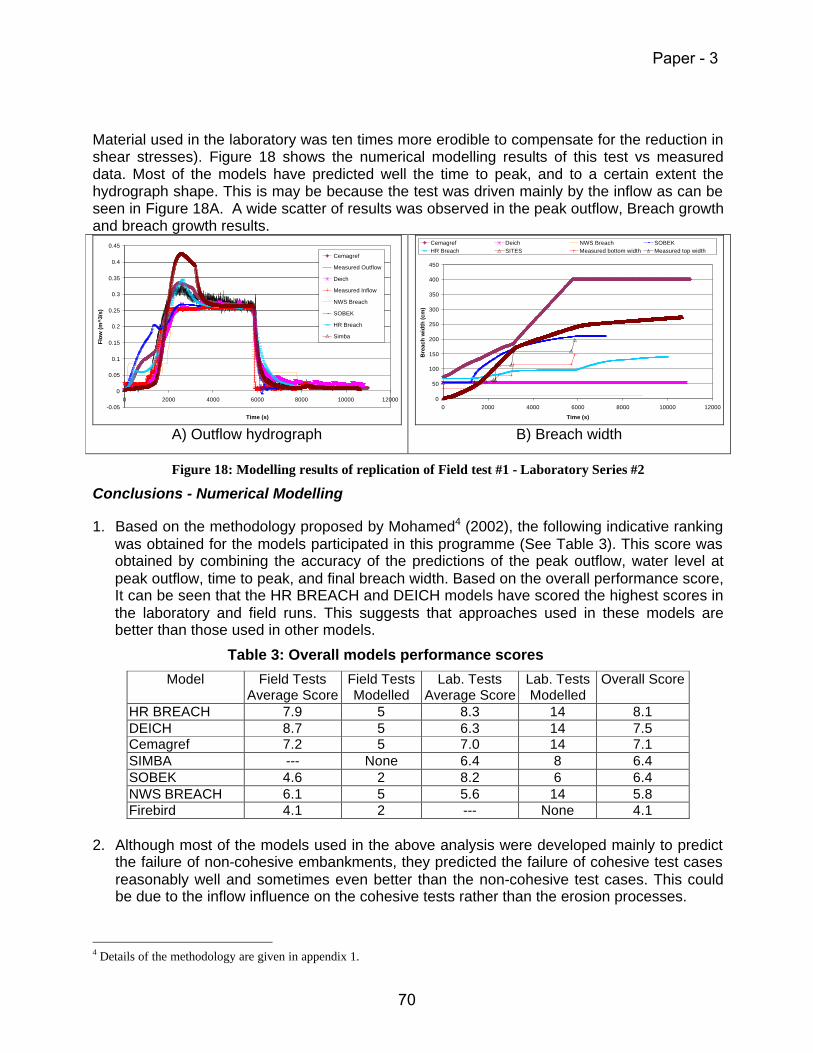
Material used in the laboratory was ten times more erodible to compensate for the reduction in shear stresses). Figure 18 shows the numerical modelling results of this test vs measured data. Most of the models have predicted well the time to peak, and to a certain extent the hydrograph shape. This is may be because the test was driven mainly by the inflow as can be seen in Figure 18A. A wide scatter of results was observed in the peak outflow, Breach growth and breach growth results.

-0.05

0

0.05

0.1

0.15

0.2

0.25

0.3

0.35

0.4

0.45

0 2000 4000 6000 8000 10000 12000

Time (s)

Flo

w (

m^3

/s)

Cemagref

Measured Outflow

Deich

Measured Inflow

NWS Breach

SOBEK

HR Breach

Simba

A) Outflow hydrograph

0

50

100

150

200

250

300

350

400

450

0 2000 4000 6000 8000 10000 12000

Time (s)B

reac

h w

idth

(cm

)

Cemagref Deich NWS Breach SOBEKHR Breach SITES Measured bottom width Measured top width

B) Breach width

Figure 18: Modelling results of replication of Field test #1 - Laboratory Series #2

Conclusions - Numerical Modelling 1. Based on the methodology proposed by Mohamed4 (2002), the following indicative ranking

was obtained for the models participated in this programme (See Table 3). This score was obtained by combining the accuracy of the predictions of the peak outflow, water level at peak outflow, time to peak, and final breach width. Based on the overall performance score, It can be seen that the HR BREACH and DEICH models have scored the highest scores in the laboratory and field runs. This suggests that approaches used in these models are better than those used in other models.

Table 3: Overall models performance scores

Model Field Tests Average Score

Field Tests Modelled

Lab. Tests Average Score

Lab. Tests Modelled

Overall Score

HR BREACH 7.9 5 8.3 14 8.1 DEICH 8.7 5 6.3 14 7.5 Cemagref 7.2 5 7.0 14 7.1 SIMBA --- None 6.4 8 6.4 SOBEK 4.6 2 8.2 6 6.4 NWS BREACH 6.1 5 5.6 14 5.8 Firebird 4.1 2 --- None 4.1

2. Although most of the models used in the above analysis were developed mainly to predict

the failure of non-cohesive embankments, they predicted the failure of cohesive test cases reasonably well and sometimes even better than the non-cohesive test cases. This could be due to the inflow influence on the cohesive tests rather than the erosion processes.

4 Details of the methodology are given in appendix 1.

Paper - 3

70

3. All models, for field and laboratory tests, have either overestimated or underestimated the breach width. This might be because most of these models were not calibrated or verified with breach growth data or this is the effect of using sediment transport equations not suitable or valid for breach test conditions.

4. The test conditions of Field Test # 2 delayed the failure of the dam by about 4 times the

time predicted by most of the models. This highlights the importance of including site specific properties when modelling the failure of embankments.

References

1. ASTM (1996). Designation: D5852-95 Standard Test Method for Erodibility Determination

of Soil in the Field or in the Laboratory by the Jet Index Method. Annual Book of ASTM (American Society for Testing and Materials) Standards, Section 4 Construction, Volume 04.09 Soil and Rock.

2. Mohamed, M. (2002). Embankment Breach Formation and Modelling Methods. PhD. Thesis, The Open University.

Appendix 1: Numerical modelling scoring system Model performance is judged by a category and score. Based on the difference in percentage between the measured and predicted values, the following categories are suggested: 1. Very Good Performance. 2. Good Performance 3. Reasonable Performance 4. Satisfactory Performance 5. Unsatisfactory Performance 6. Inadequate Performance

These categories overlap as shown in Figure 20. The score is a number represents the model performance and it is computed based on these categories. If the difference between the measured and the predicted data is more than ±50 %, the model performance is considered unacceptable and the score is assumed to be zero. Parameters can also be weighted according to their importance. The overall performance of the models can be calculated according to the following formula (Other terms can also be added to the above formula to take into consideration other parameters such as breach dimensions, growth rate, etc..):

......

......**

++

++=

sTsQ

sTTsQQ

s CC

CSCST (1)

where: Ts : Overall score of the model performance. SQ : Outflow of the model score. ST : Time to peak score CsQ : Outflow weighting factor. CsT : Time to peak weighting factor.

Acknowledgements The Authors wish to thank IMPACT project partners particularly André Paquier, Karl Broich, and Kjetil Vaskinn for their valuable help and the European Commission for funding this project. The Authors are also grateful for the Association of State Dam Safety Officials and the

Figure 19: Model performance criteria

0

25

50

75

100

± 10% ± 20% ± 30% ± 40%

V. Good Good

Satisfactory Unsatisfactory

Reasonable

Key:

± 50%

Inadequate

10 9 8 7 6 5Score

% Diff.

% S

core

Paper - 3

71

Egyptian Ministry of Water Resources and Irrigation for their valuable support.

Paper - 3

72

CASE STUDIES AND GEOPHYSICAL METHODS

RNDr. Vojtìch Bene�, RNDr. Zuzana BoukalovÆ, RNDr. Michal Tesał, RNDr. Vojtìch Zikmund

GEO Group a.s., Czech Republic

Introduction

In recent years, due to more and more frequently occurring weather effects of extreme nature which cause disastrous floods, increased attention has been paid to inspection and maintenance of dikes. This contribution is aimed at drawing attention to the possibilities brought about by the application of geophysical methods in these activities. Analyses of databases and compiliation of existing data on the history of dike breaches and failures during particular floods (case studies) may also be of significant help in the field of flood prevention. Results of experimental geophysical measurements at selected locations in the Czech Republic are presented in this paper. These studies were performed within the framework of the EU IMPACT project (see website www.impact-project.net). This project also facilitated development of databases containing information on historical dike breaches and failures in the selected catchment areas (river basins) in Hungary and the Czech Republic.

Case Studies Experience gained by us in the Czech Republic show that inadequate attention has so far been paid to the documentation of dike breaches and failures after extensive floods. Basic data on the reasons for, and the extent and course of dike breaches are missing in the majority of the cases. Exact data are seldom known, even from the recent disastrous floods in central Europe that occurred in 1997 and 2002. The data are often incomplete and of insufficient authenticity. However, it is evident that analyses of such information, followed by appropriate adjustments and repairs of the dikes, may significantly reduce the risk of occurrence of new dike breaches and failures. We particularly talk about those dike segments where the reasons for destruction were, for example, inappropriate dike structure, inappropriate material or reduced stream channel capacity due to clogging. Furthermore, after analyzing a database, it often turned out that dike breaches in these sections had occurred repeatedly. Statistical analysis of dike breach parameters may also allow some important generalizations related to the causes and characteristics of breach in specific river basins (catchment areas). For example, it turns out that the prevailing reason for dike breach occurrences in Slovakia is liquefaction caused by seepages in the underlying beds. The main reason for dike failures in Hungary is overtopping. Entirely different mechanisms of dike breach occurrences of course require different types of preventive dike modifications. Within the framework of IMPACT project, a database of dike breach parameters has been designed and prepared for Hungarian river-basin agencies by colleagues from H-EURAqua Ltd. (contact: Eur Ing. Sándor Tóth M.Sc.E., Eur Ing. László Nagy M.Sc.E.). A database heading, presenting the monitored dike breach parameters, is shown on Fig. 1.

Paper - 4

73

Fig. 1 Breach parameters database heading

Location of the breach Breach data Origin of flood

Date river

name ba

nk

stat

ioni

ng o

f dik

e

piec

es

final

leng

th

final

dep

th b

elow

cre

st

scou

r pi

t dep

th

snow

mel

t

rain

fall

ice

jam

othe

r

dd/m

m/y

yy-h

rs

Cou

ntry

km+000m m m m

Failure mechanism Cause of breach

stability loss of embankment due to

stability loss of foundation due

to

seep

age

leak

age

sand

boil

(pip

ing)

over

topp

ing

dike

bod

y

at th

e ba

se

dike

bod

y

at th

e ba

se

satu

ratio

n

wav

e er

osio

n

scou

ring

from

wat

er s

ide

stru

ctur

e fa

ilure

delib

erat

e cu

t

slow

rapi

d

lique

fact

ion

hydr

aulic

failu

re

othe

r

not w

ell i

dent

ified

bad

mat

eria

l

bad

desi

gn

bad

cons

truc

tion

bad

mai

nten

ance

la

ck o

f app

ropr

iate

em

erge

ncy

oper

atio

n

no in

form

atio

n

Flood parameters Data on damages

The breach

was

Hb ab

ove

base

befo

re p

eak

afte

r pe

ak

Hb

belo

w p

eak

Riv

er fl

ow r

ate

Ret

urn

perio

d of

floo

d

Riv

er fl

ow v

eloc

ity

Flo

w th

roug

h br

each

(es

timat

ed m

ax.)

inun

date

d ar

ea

vict

ims

hous

es d

estr

oyed

othe

r lo

sses

estim

ated

tota

l los

s

m m m3/s yr m/s m3/s ha capita pcs M€

Paper - 4

74

Embankment parameters Soiltypes

according to BS categorisation

heig

ht o

f dik

e

cres

t wid

th

wat

er s

ide

slop

e

air

side

slo

pe

base

wid

th o

f dik

e

foundation soil

h b ñw ñpr B

dike body

depth soil

River morphology description

Remarks Literature

m m v/h v/h m m nomination

Geophysical Methods in Dike Maintenance and Monitoring At present, dike maintenance and preventive repairs are based on a system of visual inspection complemented by analyses of airborne or satellite photographs. Only rarely is the project documentation of complemented by detailed information on dike structures and material properties, i.e. information acquired by engineering-geological investigation, drilling, laboratory tests of soils, etc. The reason for this is the considerable cost of such investigation and the large extent of the dikes. However, we believe that information on the nature of materials and basic dike structure is essential for efficient failure prevention. This particularly applies to old dikes for which construction documentation is missing. Furthermore, in some countries (for example, developing countries or countries of former East Europe) we may expect low quality of construction work that may contribute to dike breach when stressed (see Fig. 2).

Fig. 2 Example of inappropriate material in the core of a damaged dike

Paper - 4

75

It is in this area that a package of geophysical methods can be of particular value. Geophysical methods provide a continuous image of physical properties of a dike body and, furthermore, this type of investigation is relatively inexpensive. Within the framework of IMPACT project, we concentrated on testing the possibilities of application of the following geophysical methods:

- geoelectric methods resistivity profiling (RP), self potential method (SP), multielectrode method (MEM), electromagnetic frequency method (EFM)

- seismic methods shallow seismic method (SSM), seismic tomography (ST), multi-channel analysis of seismic waves (MASW)

- microgravimetric method - GPR method

- geomagnetic survey, gamma-ray spectrometric survey

In order to incorporate the geophysical methods into a complex of dike prevention and maintenance, we first have to identify the effects that can be monitored by these methods. Figure 3 illustrates an approach to incorporation of geophysical methods into a dike maintenance program. From the viewpoint of dike maintenance – dike breach, timing of the action is of central importance.

- breach formation itself takes place at a time scale of hours, max. a few days. A hazardous segment is evident, application of geophysical measurements is not assumed here.

- however, except for overtopping, the remaining defects mostly show somewhat

hidden PRE-breach formation stage (for example, seepage through the underlying beds, repeated seepage at an increased water level, structure defects, etc.) which predisposes the point of future dike breach. This stage often lasts for even tens of years.

The above mentioned PRE-breach formation stage is our area of interest for the application of geophysical methods. Based on the needs of dike administrators we recommend the application of geophysical methods in three basic fields that are included in package of geophysical measurements we call a geophysical monitoring system (Fig. 3, top left). A detailed description of geophysical monitoring system methodology will be included in Final Deliverable of the IMPACT project. The basic component of the monitoring system is a database of quick testing measurements. We particularly tested the application of electromagnetic frequency method (EFM) of measurement of conductivity. It is a very promising method for assessment of properties of materials used for dike construction. Conductivity (resistivity) is closely related to changes in clay content, porosity and permeability of soils. So far, it has been mostly applied for military purposes (detection of ammunition, subsurface distribution systems,

Paper - 4

76

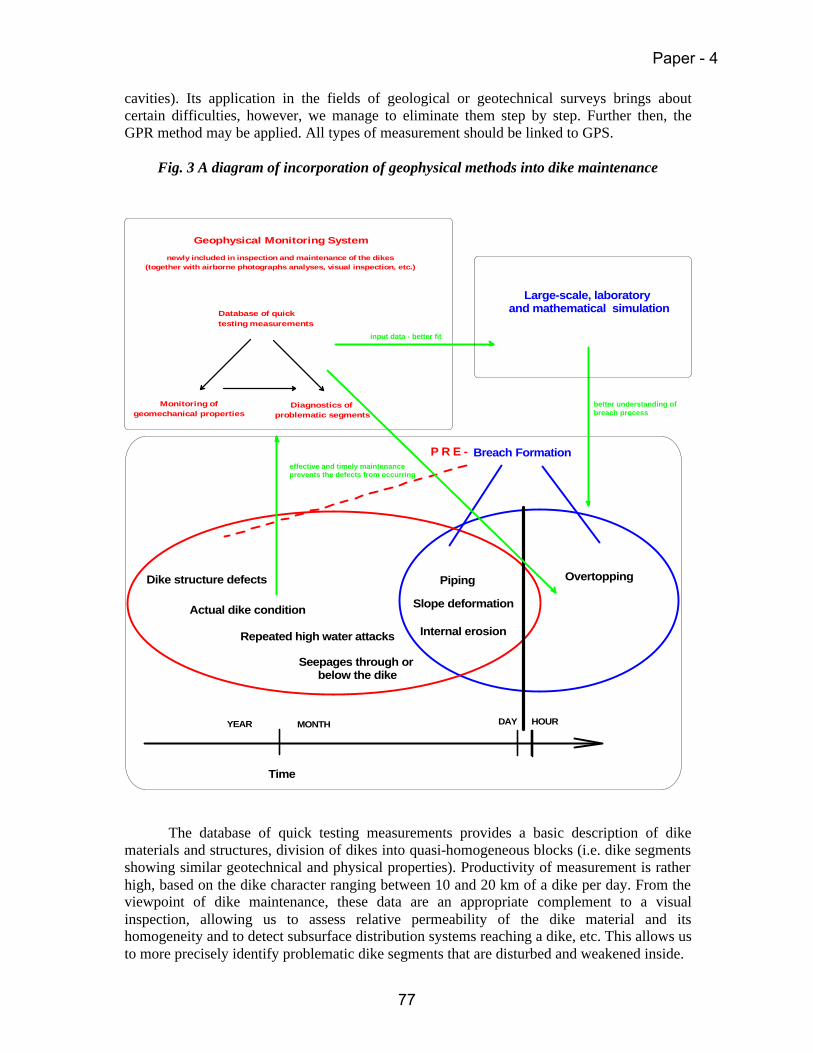
cavities). Its application in the fields of geological or geotechnical surveys brings about certain difficulties, however, we manage to eliminate them step by step. Further then, the GPR method may be applied. All types of measurement should be linked to GPS.

Fig. 3 A diagram of incorporation of geophysical methods into dike maintenance

Time

YEAR MONTH DAY HOUR

Breach Formation

OvertoppingPiping

Slope deformation

Seepages through or below the dike

Dike structure defects

Repeated high water attacks

Actual dike condition

newly included in inspection and maintenance of the dikes(together with airborne photographs analyses, visual inspection, etc.)

Large-scale, laboratory and mathematical simulation

Internal erosion

P R E -

Database of quick testing measurements

Monitoring ofgeomechanical properties

Diagnostics of problematic segments

input data - better fit

better understanding ofbreach process

effective and timely maintenance prevents the defects from occurring

Geophysical Monitoring System

The database of quick testing measurements provides a basic description of dike materials and structures, division of dikes into quasi-homogeneous blocks (i.e. dike segments showing similar geotechnical and physical properties). Productivity of measurement is rather high, based on the dike character ranging between 10 and 20 km of a dike per day. From the viewpoint of dike maintenance, these data are an appropriate complement to a visual inspection, allowing us to assess relative permeability of the dike material and its homogeneity and to detect subsurface distribution systems reaching a dike, etc. This allows us to more precisely identify problematic dike segments that are disturbed and weakened inside.

Paper - 4

77

On Fig. 4 we see a demonstration of quick testing measurement by the EFM method at the point of old breach. The breach extent (block B) is entirely evident from the resistivity curves. The curves bring resistivity information from different dike depth levels depending on the frequency applied. We see that the material used for repair shows entirely different properties (lower apparent resistivity indicating higher clay content) in comparison with the original material. For this reason, the contact (keying) of a repaired segment with the original dike can be considered hazardous. Different materials showing different levels of compressibility and absorbability may fail to tie together well, thus allowing water penetration into the gaps. Therefore, the contact between the A and B blocks has been delimitated as a hazardous/problematic dike segment.

Fig. 4 Quick testing measurement by the EFM method

Block A Block B Block C

Problematicsegment

0 20 40 60 80 100 120 140 160 180 200 220 240 260 280 300

x (m)

0

100

200

300

app

. res

itivi

ty (

ohm

m)

6325 Hz

16475 Hz

24725 Hz

35625 Hz For a detailed description of problematic segments we recommend application of a package of diagnostic methods. These are particularly MEM, SP, microgravimetric method, seismic methods and thermometry. Using a package of these methods allows us to construct a physico-geotechnical model of a problematic segment. This allows us to precisely determine the extent and intensity of dike disturbance and to draw up an optimal way of potential repair. On Fig. 5, a resistivity model of dike breach repair keying at a boundary between A and B blocks is shown. High-level material inhomogeneity of both parts has been confirmed. In addition, microgravimetric and GPR measurements has confirmed the existence of open joints between both parts (significantly increased porosity, tiny cavities). At high water level this means a risk of water penetration into the joints. Dike seepages cannot be excluded.

Paper - 4

78

Fig. 5 Diagnostic measurement by the MEM method

-5 0 5

x (m)

-4

-2

0

dept

h (m

)

-5 0 5

x (m)

-4

-2

0

dep

th (

m)

-8 -6 -4 -2 0 2 4 6 8

x (m)

-4

-2

0

dept

h (m

)

-8 -6 -4 -2 0 2 4 6 8

x (m)

-4

-2

0

dep

th (

m)

-8 -6 -4 -2 0 2 4 6 8

x (m)

-4

-2

0

dept

h (

m)

Problematic segm

ent

A special group of geophysical measurements is formed by the methods allowing us to

monitor the changes of geotechnical properties of selected dike segments (monitoring measurements). This approach can be employed, for example, in repair quality control, new dike consolidation monitoring, long-term internal erosion monitoring, etc. Here, particularly seismic methods (ST, MASW) and microgravimetry can be applied. We believe that special applications of these methods might help to better describe breach formation processes for large-scale physical models. As an example of long-term monitoring of a repaired dike segment consolidation we present on Fig. 6 the results of repeated gravity measurements. In the block A area (original, consolidated dike segment), no measurable change in material bulk density occurred during the measurement, on the other hand, block B (repaired dike segment) shows gradual consolidation.

Fig. 6 Gravimetric monitoring of consolidation

2003 2003.2 2003.4 2003.6 2003.8 2004 2004.2 2004.4

time (year)

-0.05

0

0.05

0.1

0.15

Bou

gu

er`s

an

om

aly

diff

eren

ce

2003 2003.2 2003.4 2003.6 2003.8 2004 2004.2 2004.4

time (year)

-50

0

50

100

150

den

sity

diff

eren

ce (

kg/m

)3

Change of gravity potential Change of bulk density in repaired area

out of repaired area

repaired area

Organization of Geophysical Monitoring System Within the framework of the geophysical monitoring system we assume immediate repeated quick testing measurement in the event of dike flooding. Otherwise, we assume the dike measurements will be performed in intervals of 3 years. The purpose of quick testing

Paper - 4

79

measurements will be to evaluate shape similarities of the measured resistivity curves, and/or to analyze differences in GPR records. Repeated measurement is aimed at drawing attention to new anomalous segments developed as the result of flood action or groundwater action in the dike foundation. Evaluation of repeated quick testing measurements will, of course, be followed by targeted diagnostic or monitoring measurement. The database of geophysical measurements will be administered by a specialized geophysical company cooperating with the river-basin agency. Their task will be, if necessary, to carry out a new round of monitoring measurements, to archive the data and make comparative evaluation of such data. With regard to limited duration of the IMPACT project, we could not fully prove expedience of repeated measurements at the dikes. We had an opportunity to monitor an effect of „dike flooding“ at a reservoir which is step-by-step being filled (Velký Bìlèický pond, the Czech Republic). The dam was reconstructed with a segment close to a bottom outlet completely replaced. By means of repeated measurements we monitored the process of dam material saturation with water. The main objective of the monitoring was to delimitate potential points showing increased permeability (more rapidly progressing moisture content) which might be a source of hazardous seepages in the future. The results of monitoring measurements are shown on Fig‘s. 7a and 7b. Fig. 7a shows resistivity curves acquired by the EFM method applied in the pond dam axis during the pond filling (October 2003 – 0 % of water level, December 2003 – 50 % of water level, April 2004 – 100 % of water level). Resistivity curves are standardized to the resistivity values corresponding to 25 % and 75 % of Min / Max ratio in the analyzed segment. In this way we limit the effect of weather conditions at the locality on the measured data. In other words, the purpose of interpretation of repeated measurements of conductivity is not to compare the absolute values, but the shapes of measured curves (relative anomalies). We see that the curves from October 2003 and December 2003 do not show significant deviations. However, a difference is evident for the curve from April 2004 (100 % of water level in the reservoir), where we can see a local decline of relative resistivities close to the interval between m 60 and m 90. This is a part of the dam that was fully reconstructed. We see a showing of new material saturation with water in the process of the pond water level increasing. We would probably record a similar effect if long-term seepages through a dike were monitored. A more precise description of where seepage occurs in a dike is provided by diagnostic measurement by the MEM method (Fig. 7b). The left part of Figure 7b represents changes of resistivities in a longitudinal section. The right part shows changes of resistivities in a cross-section. We can see that the most distinctive change was identified at the dam base at the points of contact with the underlying bed. In the cross-section which has a limited depth penetration due to a limited space for placing the electrodes, a showing of an anomaly corresponding to a peak of the seepage curve can be observed.

Paper - 4

80

Fig. 7a Relative resistivity anomalies detected by the EFM method at the Velký BìlŁický pond dam during filling

apparatus CM031 - September 2003

apparatus CM031 - December 2003

apparatus GEM2 - (frequency 16475 Hz)April 2004

0 20 40 60 80 100 120 140

x (m)

0

50

100

150

200

250

300re

lativ

e re

sist

ivity

an

omal

y (%

)

anomalous area

Fig. 7b Map of resistivity differences detected by the MEM method at the Velký BìlŁ ický pond dam during filling

40 60 80 100 120 140

x (m)

-10

-5

0

dep

th (

m)

40 60 80 100 120 140

x (m)

-10

-5

0

dep

th (

m)

!!!

Map of resistivity differences stage 2 minus stage 1

90 95 100 105 110

x (m)

-6

-4

-2

0

dept

h (m

)

90 95 100 105 110 115

x (m)

-6

-4

-2

0

dept

h (m

)

95 100 105 110 115

x (m)

-8

-6

-4

-2

0

dept

h (m

)

Resistivity cross-section stage 1

load bench

load bench

load bench

Map of resistivity differences stage 3 minus stage 1

Resistivity cross-section stage 2

Resistivity cross-section stage 3

Paper - 4

81

Summary

Geophysical testing measurements within the framework of the IMPACT project have proven that combination of appropriate methods brings valuable grounds for preventive repairs and maintenance of the dikes.

A suggested package of geophysical measurements for the purpose of dike prevention and maintenance we call a Geophysical Monitoring System. It is comprised of three basic fields:

A) quick testing measurement – its purpose is to provide a basic description of dike materials and structures and to delimitate quasihomogeneous blocks and potentially hazardous segments. Repeated quick testing measurement data will be stored in the database, allowing us to analyze long-term changes of the dike condition.

B) diagnostic measurement for a detailed description of problematic and disturbed dike

segments – it serves for optimal repair planning

C) monitoring measurement of changes of geotechnical parameters – it serves for repair quality control and for observation of earth structures ageing processes, etc.

Valuable information for the dike prevention from damage is also provided by analyses of

historical dike breaches in a given river-basin area. Keeping a database of dike breaches should be a routine part of dike control and maintenance.

References Beneš V., Boukalova Z., Kuthan B. (2003). Geophysical methods application in the time of benchmark experiments and tests. Project IMPACT, milestone M6.2.A – 1st stage. Beneš V., Boukalova Z., Heller (2003). Geophysical methods application in the time of benchmark experiments and tests. Project IMPACT, milestone M6.2.B – 2nd stage. Beneš V., Boukalova Z., Heller (2004). Geophysical methods application in the time of benchmark experiments and tests. Project IMPACT, milestone M6.2.C – 3rd stage. (under development) Beneš V., Boukalova Z., Heller (2004). Guidelines for application of geophysical modelling on prediction of dam failure. Project IMPACT, milestone M6.4. (under development)

Paper - 4

82

FLOOD PROPAGATION MODEL DEVELOPMENT

Francisco Alcrudo, Sandra Soares-Frazão, Yves Zech, Guido Testa, André Paquier, Jonatan Mulet, David Zuccala, Karl Broich

Abstract The prediction of the effects of the uncontrolled release of water from a structure failure

requires the ability to simulate rapidly varying flow conditions of much greater magnitude than are normally associated with natural flood propagation. Such conditions often pose difficulties for many modeling methods in commercial use and often adopt one-dimensional approximations that can limit the applicable range and description level of the flood. This often places a greater emphasis on modeler expertise in order to achieve realistic modeling results. This paper describes methods for practical computations in this area, their capabilities and limitations as well as guidelines for use. Presently, an increased interest in predicting flood characteristics in populated areas is perceived as a need within the industry. According to this, strategies adopted for the simulation of flood propagation in urban areas are described. The methods are verified against data from dedicated laboratory experiments and real flood cases, including past flooding of European urban areas.

1. Introduction

Flood propagation modeling can be defined as the art of quantitatively describing the

characteristics and evolution of the flow that is set up when a large amount of water moves along the earth surface in an uncontrolled way. Usually computers play a capital role in this art. The sizes and scales of terrestrial floods can span several orders of magnitude as the affected surface areas do. Their nature and origin can also vary, ranging from slow, reservoir-filling like inundations due to long lasting rains, to extreme, short, violent floods that can follow the failure of a dam or other control structure.

The use of computational models in flood propagation dates back to the sixties; although it has been during the last decade that thanks to the availability of high performance computers, an explosion of publications reporting the development and use of flood propagation models has occurred (Alcrudo 2002). Stringent regulations with regards to hazard and risk mitigation and management affecting dam owners, basin authorities, land use planning bodies, etc… have been slowly but constantly enforced by states worldwide for many years now. This fact may have something to do with present interest in flood propagation models.

Progress in this area is directly related to the following issues: - Understanding the flow processes relative to the problem. - Formulation of appropriate mathematical laws describing it. - Development and tuning numerical techniques to solve them. - Validation of model output against representative experimental data and real life

observations. Very important to every day engineering practice are model interfacing with other

engineering tools, such as topography and visualization software, data acquisition, and geographical information systems (GIS), that can considerably simplify and speed up problem

Paper - 5

83

set up and analysis time. Most of the models commercially in use are particularly strong on these issues; however they will not be discussed here.

Validation of the output obtained from computer simulations is one of the most important steps in model development in order to quantify the uncertainty associated with its predictions. Every effort should be made to confront model results with real life data. Since it is difficult to retrieve well-documented extreme flood events, resorting to laboratory scaled down experiments is a useful means to gain knowledge in model performance. The amount of output provided by present day models can be overwhelming and is usually analyzed by means of sophisticated graphical software that can easily lead the engineer to think that displayed information is inherently correct. A strong knowledge of a given model basic assumptions and limitations, sound judgment as well as a critical attitude is always advisable. In the following sections these issues are discussed in more detail within the particular framework of the IMPACT Research Project.

2. Mathematical models of flood propagation

2.1 Model equations

From the fluid dynamics point of view, flood propagation constitutes a formidable problem that has to be simplified by means of sensible judgment and sound approximations in order to make it mathematically tractable. Pioneering work can be traced back to the late fifties and the sixties (Isaacson et al. 1958, Cunge et al. 1964, Martin et al. 1969). Some of the models that are yet in use today appeared to the general public already in the seventies like the most well known Fread’s DAMBRK (later followed by its sequel FLDWAV, Fread 1993).

The fundamental mathematical laws that govern the phenomenon, the Navier-Stokes equations (NS), are well known. However their solution is practically impossible for the spatial and temporal scales of any real situation (see Alcrudo 2002 for a survey of potential applications of NS and simpler equations to the problem of flood propagation). This leads to the need for simplified descriptions such as the Shallow Water equations (SWE) which is presently the most widely used, despite its many shortcomings. Up to some years ago the vast majority of models available were one-dimensional (1-D) with all the limitations inherent to such approximation. A higher dimensional approach was reserved to research and academic institutions. Presently, two-dimensional (2-D) models have come to a high degree of maturity, and there are now several on the market. A two-dimensional description can provide much more information; and hence, it is quickly becoming the standard save for particular cases where the topography is very markedly 1-D.

The SWE can be derived from the NS system by a depth averaging process, or alternatively from a mass and momentum balance in the plane of motion (tangent to the earth surface) after making several assumptions:

i) Vertical velocities are neglected/not considered (therefore vertical accelerations are identically zero).

ii) The pressure field is hydrostatic. iii) The bottom slope is assumed small (such that the sinus of the slope angle can be

approximated to the angle itself). iv) A uniform horizontal velocity field is assumed across the water layer. Since the mathematical expression of the SWE can be easily found elsewhere, it will not

be included here for the sake of brevity. A real flood event implies the movement of water in the vertical direction too and

restrictions i) to iii) altogether make the SWE lack fundamental physical effects. It is likely that

Paper - 5

84

situations in which vertical movement is substantial be poorly represented in a SWE simulation. An ingenious idea within the SWE context that has been put to work recently (Zhou et al. 2002) considers the movement of the layer of fluid in a horizontal plane over a succession of a piecewise flat discontinuous bed.

It is clear that a boundary layer must extend from the bed to the free surface, and the fact that the horizontal velocity field is considered uniform across the depth of the water layer (point iv) may also be responsible for important deviations between model predictions and real observations. The effect can be shown to be analogous to shear stresses in the plane of motion, but the equivalent kinematic viscosity may be more than an order of magnitude larger than the kinematic viscosity of the fluid, thus competing with turbulence terms. Krüger et al. (1998) have derived an extended form of the SWE including a linear horizontal velocity profile plus a quadratic vertical velocity distribution and pressure correction to the hydrostatic law. Tests run by the authors on supercritical spillway flows with hydraulic jumps show consistent improvement of the modified SWE with respect to the standard model when compared with experimental data. No applications of this idea to flood propagation have been found.

The turbulent contribution to the momentum equations has not been traditionally considered an important matter. In some cases a constant eddy viscosity coefficient is used, which seems to play more the role of a tuning parameter rather than a characterization of the turbulence characteristics. As regards bed friction, empirical laws of the Manning or Chézy type, which scale with the square of the depth averaged velocities, are usually assumed.

2.2 Numerical solution of the model equations

It can be said that the numerical solution of the governing equations is the best addressed issue in latest years. This is due to a well-founded theoretical work on the solution of partial differential equations during the last two decades. The fact is that there are now plenty of numerical methods to accurately solve the equations of motion, what does not prevent ongoing research in this area.

The SWE constitute a system of partial differential equations of the hyperbolic type with two space coordinates (running roughly along the earth surface) and time as independent variables. The dependent variables are water depth and the velocity vector in the surface plane. In order to obtain a numerical solution the domain of integration must be first discretized. This is usually done separately for the space and time variables. Considering the spatial discretization, the great majority of methods fall in one of the following three categories: finite difference, finite volume and finite element. All three are being used in current models, but it seems that the finite volume approach is favored for combining the conceptual simplicity of the first category, and the flexibility of the last one.

Most numerical schemes in use today perform a separate spatial-temporal discretization, whereby the spatial derivative terms are firstly discretized, and then the resulting ordinary differential equation is integrated in time. It is now common use of formally second order accurate operators both in space and time.

Among the important issues in flood propagation stands the numerical location and propagation of wave fronts while conserving water mass. The so called shock capturing methods are capable of automatically locate and propagate fronts. This feature has made them very popular, and most models in use today include some sort of shock capturing operator. It can be said that this is now a solved problem (see Toro, 2001, for a good overview of different methods).

In practical applications, flows governed by the SWE are dominated by the source terms arising from bed slope and, in 1-D, lateral reactions. This has had a profound influence on the

Paper - 5

85

development and application of numerical methods for flood propagation: The flux discretization must be performed in a way compatible with the source term contribution. Otherwise the simulation of a mass of water initially at rest contained in a reservoir with abrupt bottom will result in the generation of unphysical movement instead of preserving the water body at rest. Appropriate source term discretizations to fix this problem were firstly developed by Bermudez and Vazquez (1994) for upwind schemes by upwinding also the source term. A collation of other strategies developed by several authors can be found in Soares-Frazão (2002).

Intrinsic to the propagation of a flood is the wetting and drying process of affected areas. Many numerical methods present an unstable behavior in the wetting-drying edge where a transition from zero to a finite depth must occur. Sometimes negative water depths are generated. The effect is severely aggravated for irregular topographies, which is usually the case in practical applications and some methods fail to propagate a flood over a dry bottom. For the sake of brevity, the reader is referred to the review by Alcrudo (2002) where original works on the subject are cited.

3. Modeling urban flooding

The modeling of flood propagation in urban areas has been perceived within the Impact

project as a source of increasing interest. The term urban flooding is understood in the context of this paper as the extreme surface inundation of areas with high density of buildings. The reason for this interest is mainly two-fold: On the one hand potential damage in urban areas is several times that in open field due to the intensity of land use; it is therefore unquestionable that industry be eager for modeling capability in that area. On the other hand present day modeling technology is capable of providing some sort of inundation prediction in urban areas and hence the induced interest. Impact project work in this area covers:

- Development of suitable strategies for urban flood modeling. - Laboratory work to learn about urban flood characteristics and gathering of

experimental data. - Field work to locate past urban flooding scenarios and collect flood data. - Model validation against laboratory and real life data. There are several modeling techniques that can be embedded within open field flood

propagation models to deal with urban inundation. The simplest approach consists of representing urban environments as areas of reduced conveyance by simply ascribing a high bed friction coefficient. Manning’s roughnesses as high as 0.5 have been reportedly used to account for the presence of a city. During Impact project work evidence suggests that friction coefficient figures are subject to scale effects that are not yet clear: They depend on building density, scale of flooded area, and ratio of flow depth to building height.

A step further is brought by the concepts of Urban Porosity and Transmissivity that are used to represent the effect that the area subject to flooding is only a fraction of the total surface area, hence affecting the mass conservation equation. This approach has been successfully used by Braschi and Gallatti (1989), who proposed the method. A disadvantage is the lack of momentum interchange between the flow and the buildings. This can be arranged via the friction term in the momentum equation by artificially increasing the roughness in the area where buildings are present as in the previous approach (Testa et al. 1998).

The increased resistance and the urban porosity approaches both provide an averaged view of the city-flood interaction; and, hence no local effects can be told from the output of

Paper - 5

86

such type of simulation. The fluid dynamics information provided can have the appearance of being local because the flow variables (water depth and velocity vector) are given for every grid point of the domain. However, they represent averaged or smeared values of those quantities over a certain surface area somehow related to the grid spacing and the building density.

These techniques are devised for two-dimensional models and are best suited for modeling large areas where it is impractical or plainly impossible to seek high resolution of topographic and flow features due to problem size. Although they could eventually be applied within one-dimensional models this does not seem natural.

There is frequently a need to know not only whether a given area is going to be flooded or not but also what local inundation conditions are likely to occur. Within Impact project, work has focused around techniques that can provide insight into local flow conditions, at the cost of higher computational cost or problem size reduction. In particular four strategies have been considered:

- A one-dimensional (1-D) treatment of the city area whereby it can be represented as a channel network (see for instance Tanguy et al. 2001).

- Friction based local representation of buildings and obstacles to flow in a two-dimensional (2-D) approach.

- 2-D topography building representation - Detailed 2-D meshing and solution of the streets and city areas, incorporating

buildings as solid walls. The first alternative is capable of providing local flow information at low computational

cost, although problem set up may require considerable work and expertise for network layout and data management. Problems may arise at junctions, in particular if these are numerous, or in wide areas where some flow features can be lost because the flow is markedly 2-D. Another difficulty of 1-D channel models lies in its interaction with larger area models. If the urban flood is the result of flooding of surrounding terrain, appropriate coupling between the urban network and the outer flood plain model is needed.

Representation of buildings as local areas with increased friction coefficient within a 2-D simulation can provide the needed resolution to capture local flow effects with little extra cost. This approach is easy to set up because local friction can be treated as another field variable, and provides reasonably accurate results. The problem lies in that buildings turn practically into local water storage tanks which is not the case in reality. Some sort of urban porosity treatment would be needed to offset this effect. Coupling the urban area with surrounding terrain subject to flooding is straightforward.

The topography based approach involves placing buildings upon the bottom representation within a 2-D calculation scheme. This can be easily done after the meshing stage of problem set up by rising the grid points that fall within a building area to the roof top elevation. Often some sort of mesh adaptation will be needed to accurately represent the city. Although buildings protrude vertically from the surface up, the discrete slope representation is not infinite but is extremely steep and depends on cell size. When flooding water reaches such adverse bed slope, its momentum is abruptly reduced; and if flow head is lower than building elevation, then it stagnates. In case flow head is large enough, water can overtop the building and it is submerged. This simple idea must be implemented with care because many numerical integration methods will not accommodate extremely steep bottom slopes as those generated with such building representation. This has also implications with the wetting and drying treatment. Further, it must be pointed out that the assumptions on which the SWE are based

Paper - 5

87

are systematically violated at the building borders. Coupling with surrounding terrain is straightforward as in previously described strategy.

Finally, the most accurate city representation can be obtained from a careful 2-D meshing of the area subject to flooding, excluding buildings from the computational domain. This can be done by blocking grid cells occupied by buildings or by meshing them around so that buildings are treated as impervious zones. The flood propagation model is then run in the void area. This method can theoretically provide the highest accuracy because the assumptions of the underlying model equations (SWE) are less likely to be violated and the topography is more accurately represented. However, the meshing procedure can be extremely complex, particularly if structured grids are used.

The techniques described above have been run and tested by Impact partners participating in flood propagation work. Their performance with respect to experimental data will be discussed in the next section.

4. Experimental data and model validation

Model validation is an unavoidable task that should be conducted in as much as

possible under controlled conditions in order that influences from different parameters are properly attributable to their true sources. This is rarely the case when validation is performed with data obtained from real life events because these seldom occur under controlled conditions; rather the opposite. During the Impact research project dedicated laboratory experiments have been conducted to get insight into flow characteristics, and complete data sets usable for model validation that are practically impossible to obtain from a real flood.

The experiments performed can be classified into two types: a) very simple geometric configurations in which the flooding is extremely idealized and b) scale physical models of actual topographies with some simplified assumptions.

Idealized situations allow focusing only on a limited number of parameters and providing interesting information on specific features. Scaled down physical models allow a more realistic representation of the flood processes but still under controlled conditions. The first type of experiments has been performed at Université Catholique de Louvain (UCL), in Louvain-La-Neuve (Belgium), and the second type at CESI (formerly ENEL-CRIS) at its Milano (Italy) facilities. Both will be more thoroughly described below.

Since laboratory data are not truly representative of actual flood events due to unavoidable scale effects and experimental simplifications, data from the extreme flood caused by Tous Dam break (Spain 1982) including the catastrophic inundation of the town of Sumacárcel have been collected and used as a case study for model validation. It is needless to say however, that real life data are not as comprehensive as experimental ones.

4.1 Experiments performed at UCL

Experimental work performed at Université Catholique de Louvain (UCL) by the team of Prof. Y. Zech comprises two idealized configurations: (i) a dam-break flow in a prismatic flume with an isolated building (Soares-Frazão et al. 2003 and 2004) hereafter called The isolated building experiment, and (ii) a dam-break flow in a prismatic flume with a submersible hill-shaped obstacle (Soares-Frazão et al. 2002), named The bump case.

The isolated building experiment was designed with the aims of firstly investigating near-field effects and secondly assessing the consequences of the presence of a building on the downstream flow. The set-up is as sketched in Figure 1, but more detailed descriptions of the experiment can be found in the cited references. Near-field effects around the building consist

Paper - 5

88

mainly in the formation of hydraulic jumps and a wake zone behind the building. Figure 2 shows a picture taken with the high-speed cameras placed above the channel, where the main flow features can be identified. After the rapid opening of the gate, the strong dam-break wave reflects against the building, almost submerging it, and the flow separates, forming a series of shock waves crossing each other. A wake zone can be identified just downstream from the building, surrounded by cross waves. The flow rapidly reaches an almost steady state with a decreasing discharge due to the emptying of the reservoir. Also, recirculation zones can be identified between the building and the walls. A flow simulation is shown in Figure 3.

Figure 1: Experimental set-up for the isolated building test case (all units are meters).

Figure 2: Picture of the flow at time t=5s after gate opening.

Experimental data recorded comprises water level and velocity vector evolution during the runs at some 6 gauging points, plus stills of the surface velocity vectors at several times.

The isolated building experiment was used to set up a benchmark named The isolated building test case, (Soares-Frazao et al. 2002) made up of two phases: The first one was of the blind type where experimental data were withheld until model results had been handed over by the participants. In the second phase, experimental data were disclosed to allow model calibration.

The blind test was run by eight different modelers from six different institutions. These modelers were both members and non-members of the IMPACT project. The participant members were (i) Noël, Soares-Frazão and Zech from the Catholic University of Louvain (Belgium), (ii) Mignot and Paquier from CEMAGREF (France), (iii) Mulet and Alcrudo from the

Paper - 5

89

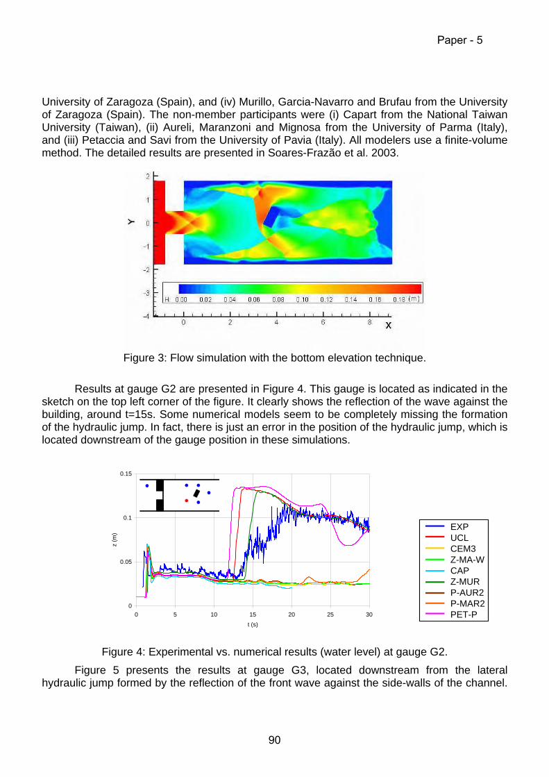
University of Zaragoza (Spain), and (iv) Murillo, Garcia-Navarro and Brufau from the University of Zaragoza (Spain). The non-member participants were (i) Capart from the National Taiwan University (Taiwan), (ii) Aureli, Maranzoni and Mignosa from the University of Parma (Italy), and (iii) Petaccia and Savi from the University of Pavia (Italy). All modelers use a finite-volume method. The detailed results are presented in Soares-Frazão et al. 2003.

Figure 3: Flow simulation with the bottom elevation technique.

Results at gauge G2 are presented in Figure 4. This gauge is located as indicated in the

sketch on the top left corner of the figure. It clearly shows the reflection of the wave against the building, around t=15s. Some numerical models seem to be completely missing the formation of the hydraulic jump. In fact, there is just an error in the position of the hydraulic jump, which is located downstream of the gauge position in these simulations.

0

0.05

0.1

0.15

0 5 10 15 20 25 30

t (s)

z (m

)

EXPUCLCEM3Z-MA-WCAPZ-MURP-AUR2P-MAR2PET-P

Figure 4: Experimental vs. numerical results (water level) at gauge G2. Figure 5 presents the results at gauge G3, located downstream from the lateral

hydraulic jump formed by the reflection of the front wave against the side-walls of the channel.

Paper - 5

90

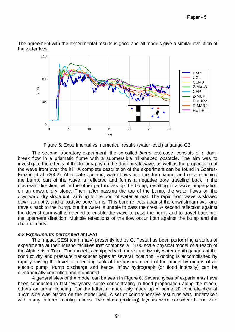
The agreement with the experimental results is good and all models give a similar evolution of the water level.

0

0.05

0.1

0.15

0 5 10 15 20 25 30t (s)

z (m

)

EXPUCLCEM3Z-MA-WCAPZ-MURP-AUR2P-MAR2PET-P

Figure 5: Experimental vs. numerical results (water level) at gauge G3. The second laboratory experiment, the so-called bump test case, consists of a dam-

break flow in a prismatic flume with a submersible hill-shaped obstacle. The aim was to investigate the effects of the topography on the dam-break wave, as well as the propagation of the wave front over the hill. A complete description of the experiment can be found in Soares-Frazão et al. (2002). After gate opening, water flows into the dry channel and once reaching the bump, part of the wave is reflected and forms a negative bore traveling back in the upstream direction, while the other part moves up the bump, resulting in a wave propagation on an upward dry slope. Then, after passing the top of the bump, the water flows on the downward dry slope until arriving to the pool of water at rest. The rapid front wave is slowed down abruptly, and a positive bore forms. This bore reflects against the downstream wall and travels back to the bump, but the water is unable to pass the crest. A second reflection against the downstream wall is needed to enable the wave to pass the bump and to travel back into the upstream direction. Multiple reflections of the flow occur both against the bump and the channel ends.

4.2 Experiments performed at CESI

The Impact CESI team (Italy) presently led by G. Testa has been performing a series of experiments at their Milano facilities that comprise a 1:100 scale physical model of a reach of the Alpine river Toce. The model is equipped with more than twenty water depth gauges of the conductivity and pressure transducer types at several locations. Flooding is accomplished by rapidly raising the level of a feeding tank at the upstream end of the model by means of an electric pump. Pump discharge and hence inflow hydrograph (or flood intensity) can be electronically controlled and monitored.

A general view of the model can be seen in Figure 6. Several types of experiments have been conducted in last few years: some concentrating in flood propagation along the reach, others on urban flooding. For the latter, a model city made up of some 20 concrete dice of 15cm side was placed on the model bed. A set of comprehensive test runs was undertaken with many different configurations. Two block (building) layouts were considered: one with

Paper - 5

91

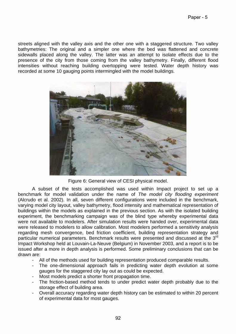
streets aligned with the valley axis and the other one with a staggered structure. Two valley bathymetries: The original and a simpler one where the bed was flattened and concrete sidewalls placed along the valley. The latter was an attempt to isolate effects due to the presence of the city from those coming from the valley bathymetry. Finally, different flood intensities without reaching building overtopping were tested. Water depth history was recorded at some 10 gauging points intermingled with the model buildings.

Figure 6: General view of CESI physical model.

A subset of the tests accomplished was used within Impact project to set up a benchmark for model validation under the name of The model city flooding experiment (Alcrudo et al. 2002). In all, seven different configurations were included in the benchmark, varying model city layout, valley bathymetry, flood intensity and mathematical representation of buildings within the models as explained in the previous section. As with the isolated building experiment, the benchmarking campaign was of the blind type whereby experimental data were not available to modelers. After simulation results were handed over, experimental data were released to modelers to allow calibration. Most modelers performed a sensitivity analysis regarding mesh convergence, bed friction coefficient, building representation strategy and particular numerical parameters. Benchmark results were presented and discussed at the 3rd Impact Workshop held at Louvain-La-Neuve (Belgium) in November 2003, and a report is to be issued after a more in depth analysis is performed. Some preliminary conclusions that can be drawn are:

- All of the methods used for building representation produced comparable results. - The one-dimensional approach fails in predicting water depth evolution at some

gauges for the staggered city lay out as could be expected. - Most models predict a shorter front propagation time. - The friction-based method tends to under predict water depth probably due to the

storage effect of building area. - Overall accuracy regarding water depth history can be estimated to within 20 percent

of experimental data for most gauges.

Paper - 5

92

Figure 7: A model city flooding test run.

A general view of one of the urban flooding test runs with a staggered city lay out and the original valley bathymetry can be seen in Figure 7, and a synthetic image representing flood wave arrival produced with a mathematical model by means of the bottom elevation technique described in previous section is shown in Figure 8.

Figure 8: Simulation of the model city flooding with the bottom elevation strategy. Finally, Figure 9 presents a comparison of the results obtained at gauges No. 5 and No.

6 located after the first and second row of buildings respectively, computed with the different building representation techniques as implemented in one particular model.

Paper - 5

93

Figure 9: Comparison of experimental data with model predictions at two gauge locations.

4.3 The Tous Dam break case study

In order to compare model predictions with real life data an effort has been made within Impact Project to locate and document an actual extreme flood that could be used for model validation. The main requirements imposed were that the flood were extreme (i.e. catastrophic), such that enough data were available to allow a reasonable modeling scenario and such that urban areas were affected in accordance with the project objectives. Several floods involving cities or towns were considered (Nîmes, France, 1988 flash flood, Florence, Italy 1966, Estes Park after Cascade Dam break, USA 1982, Sumacárcel after Tous Dam break 1982, Badajoz flash flood, Spain 1997). Tous Dam break was finally chosen representing a compromise between required characteristics and data availability.

Tous Dam, located in the Southeast of Spain, close to the Mediterranean Sea, failed in October 1982 after extremely heavy rainfall in the basin totaling 600Hm3 in three days (largely exceeding reservoir capacity) caused overtopping. The dam was of the rock fill type and stood only a few hours of overtopping. The effects of the flood downstream of Tous Dam were catastrophic: 300 km2 of inhabited land, including many towns and villages were severely flooded, affecting some 200,000 people of which 100,000 had to be evacuated, totaling 8 casualties. The first affected town is Sumacárcel (population 2000), about 5 km downstream Tous Dam, lying at the foot of a hill on the right bank of the river. The ancient part of the village, located closer to the river course was completely flooded for only a few hours, with high water marks reaching between 6m and 7m above the ground (see Figure 10).

An Impact project team gathered the available information and data from the competent bodies, local authorities, and from several field visits whereby eyewitnesses were interviewed. The collected information was indexed and described in several Impact project reports (Alcrudo and Mulet 2004) and used as a case study for the project. Modeling work is currently underway by involved partners and results and conclusions will be presented at the Impact project closing workshop to be held in Zaragoza (Spain) on the first week of November 2004.

It is interesting to note that information on the breaching process itself could also be retrieved and collated in order to make up a case study for breach formation work within the project (Mulet and Alcrudo 2004, 2004b).

Data available for model validation comprise two digital terrain models (DTM) of the area with 5m spacing: one obtained from CEDEX (Ministerio de Medio Ambiente, Spain) and

Paper - 5

94

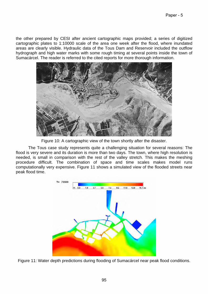
the other prepared by CESI after ancient cartographic maps provided; a series of digitized cartographic plates to 1:10000 scale of the area one week after the flood, where inundated areas are clearly visible. Hydraulic data of the Tous Dam and Reservoir included the outflow hydrograph and high water marks with some rough timing at several points inside the town of Sumacárcel. The reader is referred to the cited reports for more thorough information.

Figure 10: A cartographic view of the town shortly after the disaster.

The Tous case study represents quite a challenging situation for several reasons: The flood is very severe and its duration is more than two days. The town, where high resolution is needed, is small in comparison with the rest of the valley stretch. This makes the meshing procedure difficult. The combination of space and time scales makes model runs computationally very expensive. Figure 11 shows a simulated view of the flooded streets near peak flood time.

Figure 11: Water depth predictions during flooding of Sumacárcel near peak flood conditions.

Paper - 5

95

5. Conclusions and future trends A short review of the main issues concerning flood propagation model development has

been presented in this paper. Particular emphasis has been put on model validation where the perspective of Impact research project work has been given.

The vast majority of flood propagation models in use today are based upon the Shallow Water equations (SWE). Computational methods developed for their solution provide presently a high degree of accuracy and resolution, and it can be said that all the numerical problems encountered a few years ago are practically solved. The computer power available today makes it possible modeling the inundation of large areas with great topographical detail. This may lead to think that simply by mesh refining more accurate predictions can be made. However, this is only partially true, because the numerical solution so computed will converge to the exact solution of the SWE that is not the solution of the flooding problem itself. It could be said that the main reason for the lack of agreement between experimental measurements and a careful and well resolved model simulation is the inadequacy of the SWE formulation to describe flood flow. Nevertheless, it is the view of the authors that there is yet some room for improvement still within the SWE framework: Vertical slopes should be accommodated within the models and the influence of diffusion terms needs some clarification. In any case more elaborate mathematical descriptions of free surface flow, that is the basis of flood propagation models, are not yet ready for practical use nor is it expected that they will be so in the near future.

In the meanwhile validation is a sure path to gain confidence in model predictions. Routine application of models to real world floods will help sort out strategies and algorithms that perform well in idealized situations or against laboratory experimental data, but may encounter operational problems in real life applications.

The future is challenging because it is perceived that industry interest in flood propagation models grows at the same pace as modeling technology advances, and current models are accurate enough to make useful predictions of the effects of extreme inundations.

6. Acknowledgements

The authors wish to acknowledge the financial support provided by the European

Commission for the IMPACT project, under the Fifth Framework Program (1998-2002), Environment and Sustainable Development Thematic Program, EVG1-2001-00017, for which Karen Fabbri was the EC project officer. The first author would like to acknowledge the funding provided by the Spanish Ministerio de Ciencia y Tecnología through project BFM2000-1053.

7. References

1. Alcrudo, F., A state of the art review on mathematical modeling of flood propagation,

Proceedings 1st IMPACT Project Workshop, Wallingford, UK, 16-17 May 2002 (CD-ROM). It can be found at http://www.samui.co.uk/impact-project/cd2/default.htm.

2. Alcrudo, F., Testa, G., Zuccalá, D., García, P., Brufau P., Murillo, J., García, D., Mulet, J., (2002), The model city flooding experiment, Internal IMPACT Project Report. It can be found at http://www.samui.co.uk/impact-project/wp3_benchmarking2.htm.

3. Alcrudo, F., Mulet, F., (2004), IMPACT Project Flood Propagation Case Study: The Flooding of Sumacárcel after Tous Dam Break. IMPACT project internal report. 2004.

Paper - 5

96

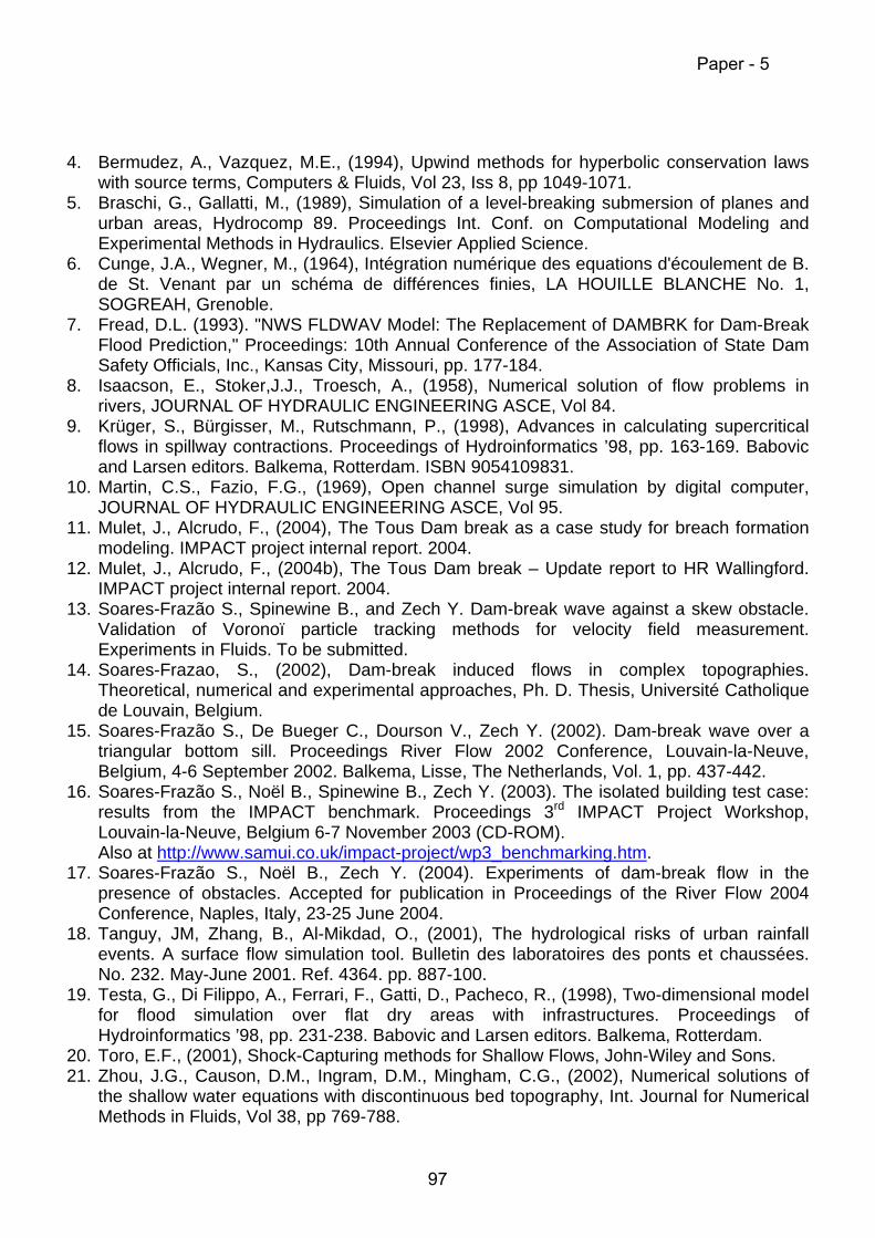
4. Bermudez, A., Vazquez, M.E., (1994), Upwind methods for hyperbolic conservation laws with source terms, Computers & Fluids, Vol 23, Iss 8, pp 1049-1071.

5. Braschi, G., Gallatti, M., (1989), Simulation of a level-breaking submersion of planes and urban areas, Hydrocomp 89. Proceedings Int. Conf. on Computational Modeling and Experimental Methods in Hydraulics. Elsevier Applied Science.

6. Cunge, J.A., Wegner, M., (1964), Intégration numérique des equations d'écoulement de B. de St. Venant par un schéma de différences finies, LA HOUILLE BLANCHE No. 1, SOGREAH, Grenoble.

7. Fread, D.L. (1993). "NWS FLDWAV Model: The Replacement of DAMBRK for Dam-Break Flood Prediction," Proceedings: 10th Annual Conference of the Association of State Dam Safety Officials, Inc., Kansas City, Missouri, pp. 177-184.

8. Isaacson, E., Stoker,J.J., Troesch, A., (1958), Numerical solution of flow problems in rivers, JOURNAL OF HYDRAULIC ENGINEERING ASCE, Vol 84.

9. Krüger, S., Bürgisser, M., Rutschmann, P., (1998), Advances in calculating supercritical flows in spillway contractions. Proceedings of Hydroinformatics ’98, pp. 163-169. Babovic and Larsen editors. Balkema, Rotterdam. ISBN 9054109831.

10. Martin, C.S., Fazio, F.G., (1969), Open channel surge simulation by digital computer, JOURNAL OF HYDRAULIC ENGINEERING ASCE, Vol 95.

11. Mulet, J., Alcrudo, F., (2004), The Tous Dam break as a case study for breach formation modeling. IMPACT project internal report. 2004.

12. Mulet, J., Alcrudo, F., (2004b), The Tous Dam break – Update report to HR Wallingford. IMPACT project internal report. 2004.

13. Soares-Frazão S., Spinewine B., and Zech Y. Dam-break wave against a skew obstacle. Validation of Voronoï particle tracking methods for velocity field measurement. Experiments in Fluids. To be submitted.

14. Soares-Frazao, S., (2002), Dam-break induced flows in complex topographies. Theoretical, numerical and experimental approaches, Ph. D. Thesis, Université Catholique de Louvain, Belgium.

15. Soares-Frazão S., De Bueger C., Dourson V., Zech Y. (2002). Dam-break wave over a triangular bottom sill. Proceedings River Flow 2002 Conference, Louvain-la-Neuve, Belgium, 4-6 September 2002. Balkema, Lisse, The Netherlands, Vol. 1, pp. 437-442.

16. Soares-Frazão S., Noël B., Spinewine B., Zech Y. (2003). The isolated building test case: results from the IMPACT benchmark. Proceedings 3rd IMPACT Project Workshop, Louvain-la-Neuve, Belgium 6-7 November 2003 (CD-ROM).

Also at http://www.samui.co.uk/impact-project/wp3_benchmarking.htm. 17. Soares-Frazão S., Noël B., Zech Y. (2004). Experiments of dam-break flow in the

presence of obstacles. Accepted for publication in Proceedings of the River Flow 2004 Conference, Naples, Italy, 23-25 June 2004.

18. Tanguy, JM, Zhang, B., Al-Mikdad, O., (2001), The hydrological risks of urban rainfall events. A surface flow simulation tool. Bulletin des laboratoires des ponts et chaussées. No. 232. May-June 2001. Ref. 4364. pp. 887-100.

19. Testa, G., Di Filippo, A., Ferrari, F., Gatti, D., Pacheco, R., (1998), Two-dimensional model for flood simulation over flat dry areas with infrastructures. Proceedings of Hydroinformatics ’98, pp. 231-238. Babovic and Larsen editors. Balkema, Rotterdam.

20. Toro, E.F., (2001), Shock-Capturing methods for Shallow Flows, John-Wiley and Sons. 21. Zhou, J.G., Causon, D.M., Ingram, D.M., Mingham, C.G., (2002), Numerical solutions of

the shallow water equations with discontinuous bed topography, Int. Journal for Numerical Methods in Fluids, Vol 38, pp 769-788.

Paper - 5

97

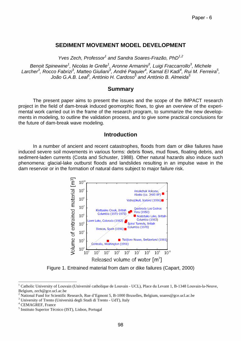
SEDIMENT MOVEMENT MODEL DEVELOPMENT

Yves Zech, Professor1 and Sandra Soares-Frazão, PhD1,2

Benoit Spinewine1, Nicolas le Grelle1, Aronne Armanini3, Luigi Fraccarrollo3, MicheleLarcher3, Rocco Fabrizi3, Matteo Giuliani3, André Paquier4, Kamal El Kadi4, Rui M. Ferreira5,

João G.A.B. Leal5, António H. Cardoso5 and António B. Almeida5

Summary

The present paper aims to present the issues and the scope of the IMPACT researchproject in the field of dam-break induced geomorphic flows, to give an overview of the experi-mental work carried out in the frame of the research program, to summarize the new develop-ments in modeling, to outline the validation process, and to give some practical conclusions forthe future of dam-break wave modeling.

Introduction

In a number of ancient and recent catastrophes, floods from dam or dike failures haveinduced severe soil movements in various forms: debris flows, mud flows, floating debris, andsediment-laden currents (Costa and Schuster, 1988). Other natural hazards also induce suchphenomena: glacial-lake outburst floods and landslides resulting in an impulse wave in thedam reservoir or in the formation of natural dams subject to major failure risk.

Figure 1. Entrained material from dam or dike failures (Capart, 2000)

1 Catholic University of Louvain (Université catholique de Louvain - UCL), Place du Levant 1, B-1348 Louvain-la-Neuve,Belgium, zech@gce.ucl.ac.be2 National Fund for Scientific Research, Rue d’Egmont 5, B-1000 Bruxelles, Belgium, soares@gce.ucl.ac.be3 University of Trento (Università degli Studi di Trento - UdT), Italy4 CEMAGREF, France5 Instituto Superior Técnico (IST), Lisbon, Portugal

Paper - 6

98

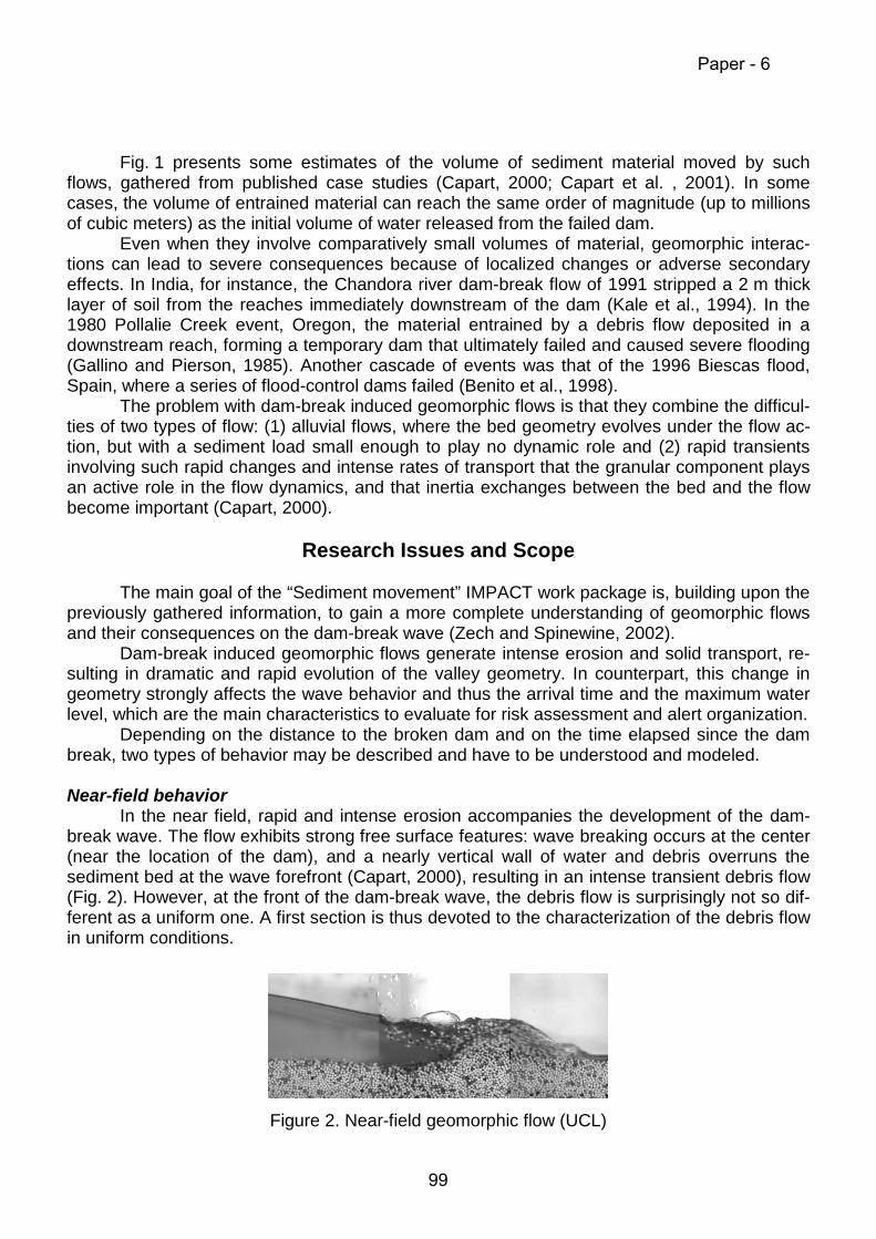
Fig. 1 presents some estimates of the volume of sediment material moved by suchflows, gathered from published case studies (Capart, 2000; Capart et al. , 2001). In somecases, the volume of entrained material can reach the same order of magnitude (up to millionsof cubic meters) as the initial volume of water released from the failed dam.

Even when they involve comparatively small volumes of material, geomorphic interac-tions can lead to severe consequences because of localized changes or adverse secondaryeffects. In India, for instance, the Chandora river dam-break flow of 1991 stripped a 2 m thicklayer of soil from the reaches immediately downstream of the dam (Kale et al., 1994). In the1980 Pollalie Creek event, Oregon, the material entrained by a debris flow deposited in adownstream reach, forming a temporary dam that ultimately failed and caused severe flooding(Gallino and Pierson, 1985). Another cascade of events was that of the 1996 Biescas flood,Spain, where a series of flood-control dams failed (Benito et al., 1998).

The problem with dam-break induced geomorphic flows is that they combine the difficul-ties of two types of flow: (1) alluvial flows, where the bed geometry evolves under the flow ac-tion, but with a sediment load small enough to play no dynamic role and (2) rapid transientsinvolving such rapid changes and intense rates of transport that the granular component playsan active role in the flow dynamics, and that inertia exchanges between the bed and the flowbecome important (Capart, 2000).

Research Issues and Scope

The main goal of the “Sediment movement” IMPACT work package is, building upon thepreviously gathered information, to gain a more complete understanding of geomorphic flowsand their consequences on the dam-break wave (Zech and Spinewine, 2002).

Dam-break induced geomorphic flows generate intense erosion and solid transport, re-sulting in dramatic and rapid evolution of the valley geometry. In counterpart, this change ingeometry strongly affects the wave behavior and thus the arrival time and the maximum waterlevel, which are the main characteristics to evaluate for risk assessment and alert organization.

Depending on the distance to the broken dam and on the time elapsed since the dambreak, two types of behavior may be described and have to be understood and modeled.

Near-field behaviorIn the near field, rapid and intense erosion accompanies the development of the dam-

break wave. The flow exhibits strong free surface features: wave breaking occurs at the center(near the location of the dam), and a nearly vertical wall of water and debris overruns thesediment bed at the wave forefront (Capart, 2000), resulting in an intense transient debris flow(Fig. 2). However, at the front of the dam-break wave, the debris flow is surprisingly not so dif-ferent as a uniform one. A first section is thus devoted to the characterization of the debris flowin uniform conditions.

Figure 2. Near-field geomorphic flow (UCL)

Paper - 6

99

Behind the debris-flow front, the behavior seems completely different: inertial effectsand bulking of the sediments may play a significant role. Surprisingly, such a difficult featureappears to be suitably modeled by a two-layer model based on the shallow-water assumptionsand methods. The second section relates experiments, modeling and validation of this near-field behavior.

Far-field behaviorIn the far field, the solid transport remains intense, but the dynamic role of the sedi-

ments decreases. On the other hand, dramatic geomorphic changes occur in the valley due tosediment de-bulking, bank erosion, and debris deposition (Fig. 3). The third section is devotedto experiments, modeling, and validation of the far-field behavior.

Figure 3. Dam-break consequences in the far fieldLake Ha!Ha! 1996 dam break (Brooks and Lawrence, 1999)

Debris flow in uniform conditions

Iverson (1997) reports some interesting information about various debris-flow events inUSA, Peru, Colombia, and New Zealand. The main characteristics of this type of event are theinvolved volume, the run-out distance (sometimes hundredths of kilometers), the descentheight (till 6000 m in the quoted examples), and the origin of the debris flow (mainly landslidesand volcanic events).

A debris-flow also occurs at the front of a dam-break wave, if the latter happens on mo-bile bed and/or banks. In this case, a high amount of sediments is generally mobilized, induc-ing a vertical velocity component able to form a kind of plug at the front of the wave.

Experimental works (University of Trento UdT)To investigate the vertical structure of free-surface liquid-granular flows, it is of particular

interest to be able to materialize steady uniform flow conditions. A re-circulating flume was de-signed and constructed for this purpose at the Università degli Studi di Trento, Italy. It consistsin a tilting glass-walled channel linked with a conveyer belt, forming a closed loop for the cir-culation of both water and sediment (Fig. 4).

Paper - 6

100

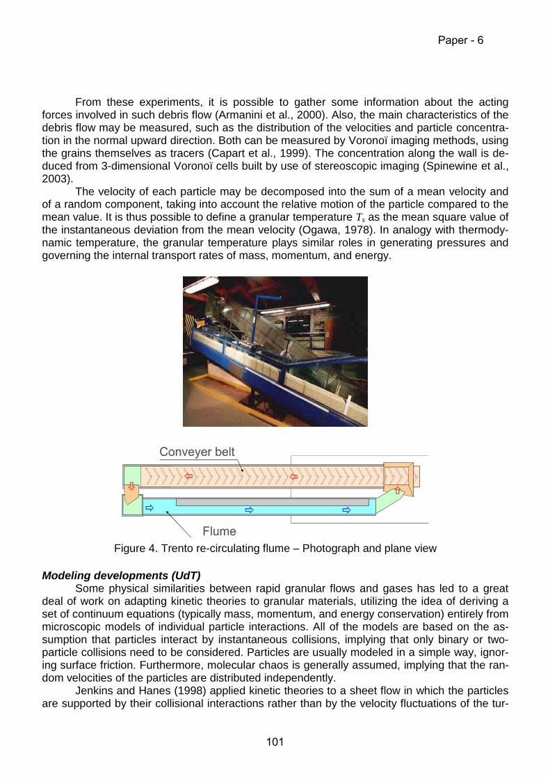
From these experiments, it is possible to gather some information about the actingforces involved in such debris flow (Armanini et al., 2000). Also, the main characteristics of thedebris flow may be measured, such as the distribution of the velocities and particle concentra-tion in the normal upward direction. Both can be measured by Voronoï imaging methods, usingthe grains themselves as tracers (Capart et al., 1999). The concentration along the wall is de-duced from 3-dimensional Voronoï cells built by use of stereoscopic imaging (Spinewine et al.,2003).

The velocity of each particle may be decomposed into the sum of a mean velocity andof a random component, taking into account the relative motion of the particle compared to themean value. It is thus possible to define a granular temperature Ts as the mean square value ofthe instantaneous deviation from the mean velocity (Ogawa, 1978). In analogy with thermody-namic temperature, the granular temperature plays similar roles in generating pressures andgoverning the internal transport rates of mass, momentum, and energy.

Figure 4. Trento re-circulating flume – Photograph and plane view

Modeling developments (UdT)Some physical similarities between rapid granular flows and gases has led to a great

deal of work on adapting kinetic theories to granular materials, utilizing the idea of deriving aset of continuum equations (typically mass, momentum, and energy conservation) entirely frommicroscopic models of individual particle interactions. All of the models are based on the as-sumption that particles interact by instantaneous collisions, implying that only binary or two-particle collisions need to be considered. Particles are usually modeled in a simple way, ignor-ing surface friction. Furthermore, molecular chaos is generally assumed, implying that the ran-dom velocities of the particles are distributed independently.

Jenkins and Hanes (1998) applied kinetic theories to a sheet flow in which the particlesare supported by their collisional interactions rather than by the velocity fluctuations of the tur-

Paper - 6

101

bulent fluid. The purpose of their analysis is the prediction of mean fluid velocity, particle con-centration, and granular temperature profiles obtained as solutions of the balance equations offluid and particle momentum and particle fluctuation energy. The flow of the mixture of particlesand fluid is assumed to be, on average, steady and fully developed. The grains are taken to beidentical spherical particles of diameter D composed of a material of mass density ρs. The fluidis assumed to have a mass density ρw . The constitutive relation for the particle pressure istaken to be the quasi-elastic approximation for a dense molecular gas proposed by Chapmanand Cowling (1970):

( ) ss

sssss T

CC

CC

−−

+ρ=σ 3122

41 (1)

where Cs is the grain concentration, the fraction (2- Cs)/2(1- Cs)3 is the radial distribution functionat contact, describing the variation with concentration of the rate of collisions among the parti-cles. In the same way, the constitutive relation for the particle shear stress is taken:

( )( )( ) dz

duCC

CT

CC

CDss

ss

s

ssss

−

−+π+

−−

ρπ

=τ23

213

221 2

12851

121

122

58 (2)

From experiments, it is possible to derive σs and τs by assuming that the buoyant weightof the grains is entirely supported by collisional granular contacts.

In Fig. 5 comparison is made between so-derived experimental results and the theoreti-cal relations in Eq. 1 and Eq. 2 (blue lines). A better fit is obtained by accounting for an added-mass effect by replacing ρs in Eq. 1 and Eq. 2 by:

( )

ρρ

−+

+ρ=ρs

w

s

sss C

C12

211' (3)

resulting in the red line in Fig. 5. More details can be found in Armanini et al. (2003).

Figure 5: Particle pressure and shear stress: points represent experimental results,blue line theoretical kinetic relation, red line accounting for added mass effect

Paper - 6

102

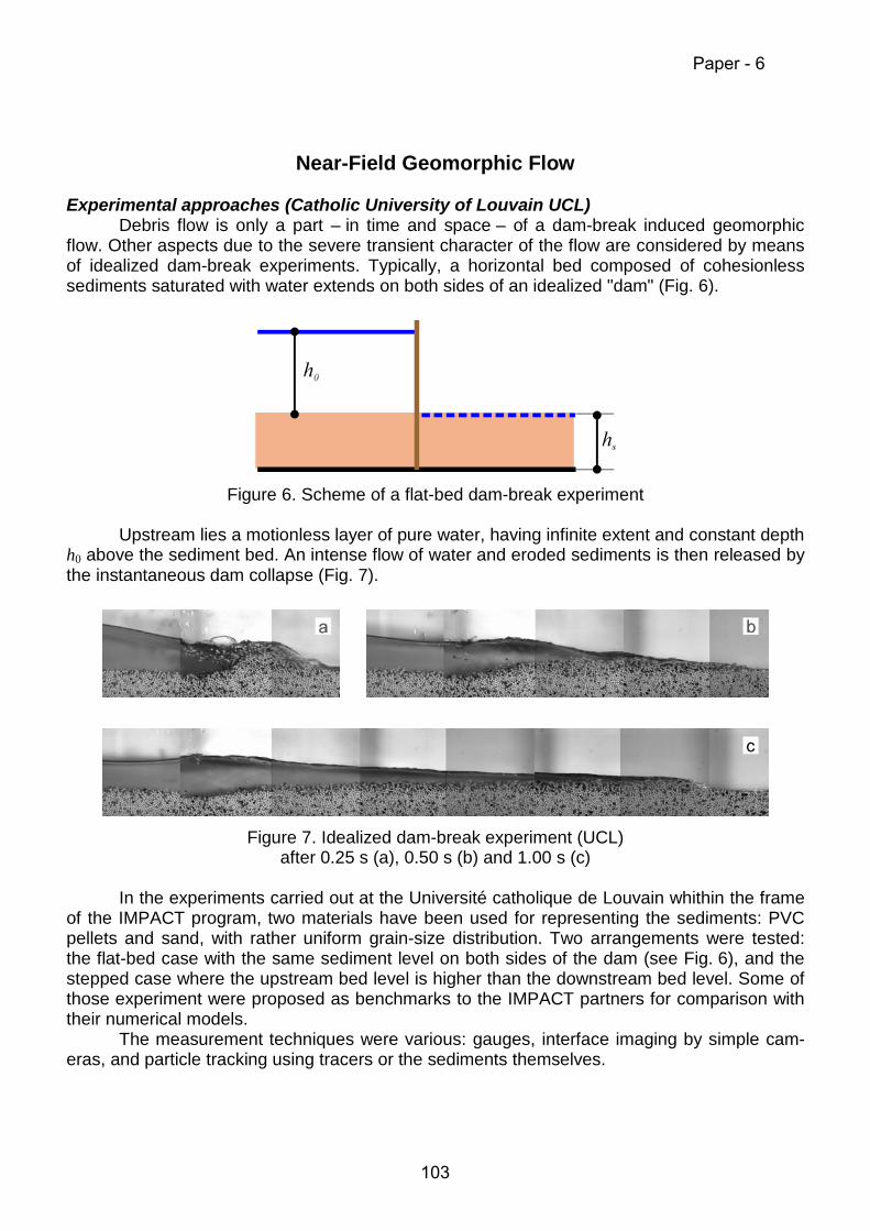
Near-Field Geomorphic Flow

Experimental approaches (Catholic University of Louvain UCL)Debris flow is only a part – in time and space – of a dam-break induced geomorphic

flow. Other aspects due to the severe transient character of the flow are considered by meansof idealized dam-break experiments. Typically, a horizontal bed composed of cohesionlesssediments saturated with water extends on both sides of an idealized "dam" (Fig. 6).

Figure 6. Scheme of a flat-bed dam-break experiment

Upstream lies a motionless layer of pure water, having infinite extent and constant depthh0 above the sediment bed. An intense flow of water and eroded sediments is then released bythe instantaneous dam collapse (Fig. 7).

Figure 7. Idealized dam-break experiment (UCL)after 0.25 s (a), 0.50 s (b) and 1.00 s (c)

In the experiments carried out at the Université catholique de Louvain whithin the frameof the IMPACT program, two materials have been used for representing the sediments: PVCpellets and sand, with rather uniform grain-size distribution. Two arrangements were tested:the flat-bed case with the same sediment level on both sides of the dam (see Fig. 6), and thestepped case where the upstream bed level is higher than the downstream bed level. Some ofthose experiment were proposed as benchmarks to the IMPACT partners for comparison withtheir numerical models.

The measurement techniques were various: gauges, interface imaging by simple cam-eras, and particle tracking using tracers or the sediments themselves.

Paper - 6

103

Numerical modeling development (UCL)The near-field modeling generally relies on numerical methods, since analytical solu-

tions (Fraccarollo and Capart, 2002), whilst clever, cannot take into consideration real-casegeometry.

Fig. 8 illustrates a simplified but fruitful approach to the problem (Spinewine, 2003;Spinewine and Zech, 2002a). Three zones are defined: the upper layer (hw) is clear water whilethe lower layers are composed of a mixture of water and sediments. In the original model (Ca-part, 2000), the concentration of sediment was assumed to be constant (Cs = Cb) and the upperpart of this mixture (hs) was assumed to be in movement with the same uniform velocity as theclear-water layer (us = uw). According to those assumptions the shear stress was supposed ascontinuous along a vertical line.

One of the main improvements brought to the model is to give new degrees of freedomto concentrations (Cs ≠ Cb) and velocities (us ≠ uw) between the three layers.

In the frame of shallow-water approach, it is now possible to express the continuity ofboth the sediments and the mixture and also the momentum conservation with the additionalassumption that the pressure is hydrostaticaly distributed in the moving layers, which impliesthat no vertical movement is taken into consideration:

Figure 8. Assumptions for mathematical description of near-field flow

( )s

sbbww

w

CCCeuh

xth −−=

∂∂+

∂∂ (4a)

( )s

bbss

s

CC

euhxt

h=

∂∂+

∂∂

(4b)

bb etz −=

∂∂ (4c)

( )

<>−−−=+

∂∂+

+

∂∂+

∂∂

0 if 0 if

2)( 2

2

bs

bw

s

sbb

w

wsbw

www

ww

eueu

CCCehz

xghghuh

xtuh

ρτ (5a)

<>−+−=

∂∂+

∂∂+

+

∂∂+

∂∂

0 if 0 if

.2

)( 22

bs

bwb

s

sb

s

w

s

b

s

ww

s

wbs

sss

ss

eueu

eC

CCxh

xzghghuh

xtuh

ρρ

ρτ

ρτ

ρρ (5b)

where eb is the erosion rate (negative is the case of deposition), resulting from the inequalitybetween the shear stresses τs and τb on both faces of the bed interface:

Paper - 6

104

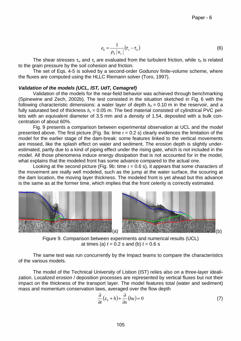
( )bssb

b ue ττ

ρ−= 1 (6)

The shear stresses τw and τs are evaluated from the turbulent friction, while τb is relatedto the grain pressure by the soil cohesion and friction.

The set of Eqs. 4-5 is solved by a second-order Godunov finite-volume scheme, wherethe fluxes are computed using the HLLC Riemann solver (Toro, 1997).

Validation of the models (UCL, IST, UdT, Cemagref)Validation of the models for the near-field behavior was achieved through benchmarking

(Spinewine and Zech, 2002b). The test consisted in the situation sketched in Fig. 6 with thefollowing characteristic dimensions: a water layer of depth h0 = 0.10 m in the reservoir, and afully saturated bed of thickness hs = 0.05 m. The bed material consisted of cylindrical PVC pel-lets with an equivalent diameter of 3.5 mm and a density of 1.54, deposited with a bulk con-centration of about 60%.

Fig. 9 presents a comparison between experimental observation at UCL and the modelpresented above. The first picture (Fig. 9a: time t = 0.2 s) clearly evidences the limitation of themodel for the earlier stage of the dam-break: some features linked to the vertical movementsare missed, like the splash effect on water and sediment. The erosion depth is slightly under-estimated, partly due to a kind of piping effect under the rising gate, which is not included in themodel. All those phenomena induce energy dissipation that is not accounted for in the model,what explains that the modeled front has some advance compared to the actual one.

Looking at the second picture (Fig. 9b: time t = 0.6 s), it appears that some characters ofthe movement are really well modeled, such as the jump at the water surface, the scouring atthe dam location, the moving layer thickness. The modeled front is yet ahead but this advanceis the same as at the former time, which implies that the front celerity is correctly estimated.

(a) (b)Figure 9. Comparison between experiments and numerical results (UCL)

at times (a) t = 0.2 s and (b) t = 0.6 s

The same test was run concurrently by the Impact teams to compare the characteristicsof the various models.

The model of the Technical University of Lisbon (IST) relies also on a three-layer ideali-zation. Localized erosion / deposition processes are represented by vertical fluxes but not theirimpact on the thickness of the transport layer. The model features total (water and sediment)mass and momentum conservation laws, averaged over the flow depth

( ) ( ) 0=∂∂++

∂∂ hu

xhz

t b (7)

Paper - 6

105

( ) ( ) ( ) ( ) bb

sswwsssswwwwwssswwwm xzhhghhhhhh

xghuhu

xuh

tτ−

∂∂ρ+ρ−=ρ+ρ+ρ

∂∂+ρ+ρ

∂∂+ρ

∂∂ 2222 2

21 (8)

and mass conservation equations of the transport layer and of the bed, respectively:

( ) ( ) ssssss uhCx

hCt

Φ=∂∂+

∂∂ (9)

( ) sb

tz

Φ−=∂

∂ε− 01 (10)

where h = hs + hw, u = (ushs+ uwhw)/h represent the average velocity of the moving layers (whosethickness are hs and hw, respectively), τb is the bed shear stress, ρm is the mean density of thelayers such that ρm h u = ρw hw uw+ ρs hs us, ρs = ρw(1+(s−1)Cs) is the transport layer density, ε0 isthe porosity, and Φs is the flux between the bed and the transport layer.

In the IST model the dependent variables are h, u, zb and Cs. Closure equations are re-quired for: hs, derived from the equation of conservation of granular kinetic energy; us, averagedfrom a power-law distribution; τb, quadratic dependence on the shear rate; and Φs, dependingon the imbalance between capacity and actual transport. Further details can be found in Fer-reira et al. (2003) and Leal et al. (2003).

The model used by the University of Trento (Fraccarollo et al., 2003) considers constantconcentration of sediment (Cs = Cb), and the upper part of this mixture (hs) is assumed to be inmovement with the same uniform velocity as the clear-water layer (us = uw = u) in such a waythat Eq. 4a-c may be combined in the following way:

( ) ( )[ ] 0=+∂∂+++

∂∂ uhh

xhhz

t wswsb (11a)

( ) ( )[ ] 0=+∂∂++

∂∂ uhh

xhz

t wssb (11b)

and Eq. 5a-b are merged in the following form, where h = hs + hw and r = (s–1)Cs with s = ρs/ρw,the latter being the density supplement due to the presence of the sediment load.

( )[ ] ( )[ ] ( )w

bbssss x

zrhhghgrhgurhh

xurhh

t ρτ

−=∂∂

+++++∂∂++

∂∂ 2

212

212 (12)

The Cemagref model RubarBE (El Kadi and Paquier, 2003) relies on the classical Saint-Venant equations extended to the whole cross section:

0=∂∂+

∂∂

xQ

tA (13)

fw Sgx

zgA

AQ

xtQ −=

∂∂

+

∂∂+

∂∂ 2

(14)

where A and Q are the section area and the discharge, zw is the water level, and Sf the frictionslope. The conservation of bed material is expressed by the Exner equation, very similar toEq. 10:

( ) 01 0 =∂

∂+

∂∂

ε−x

Qt

A ss (15)

where As is the bed material area and Qs the solid discharge. Only the water layer is taken intoconsideration, and the closure of the system is made by the solid discharge.

Paper - 6

106

The comparison of the various models with the experimental data is made in Fig. 10.Regarding the front celerity the results by Trento (UdT) take advantage of the calibration proc-ess, which involves these celerity as a calibration parameter. In contrast, their moving sedi-ment layer is underestimated, due to the fact that the concentration of this layer is assumed tobe the same as the bed material, which is not the case of the Louvain (UCL) and Lisbon (IST)models: in the reality, the concentration of this moving layer has to decrease to allow themovement of the particles. The erosion due to the front mobilization only appears in the Lou-vain and Cemagref (CEM) models. Even though Cemargref’s simple model cannot provide anyresults for the moving sediment layer, it still yields a valuable estimate for the water surfaceafter the shock. The asymmetric treatment of erosion and deposition in Eq. 6 could explain thesuccess for the UCL model in this regard.

-0.2

0

0.2

0.4

0.6

0 4 8 12 16 20

EXPCEMUdTUCLIST

0hz

0hgt

Figure 10. Comparison between experimental and numerical results from the benchmarkon dam-break wave over an initially flat erodible bed at x = 5 h0. For each set of results, the

lower line corresponds to the fixed bed level, the middle line to the moving sediment layer andthe upper line to the water surface

Channel alteration in the far field

The transition between near-field and far-field behavior is not absolutely clear. The de-bris-flow front resulting from the early stage of dam-break forms a kind of obstacle, which isprogressively subject to piping and overtopping. That means that a sediment de-bulking oc-curs, and the solid transport evolves to a bed- and suspended-load transport with a particularlyhigh concentration. The flow is highly transient and invades a part of the valley that was proba-bly never inundated in the past. All the bank geotechnical equilibrium characteristics are ru-ined, in such a way that a dramatic channel metamorphosis may be expected. This corre-sponds to the so-called far-field behavior.

A spectacular channel widening generally occurs due to bank scouring and collapse(see Fig. 3). This eroded material over-supplies the bed-load transport resulting in bed deposi-tion and eventual generation of natural dams in the downstream reaches, which may rapidlycollapse.

Paper - 6

107

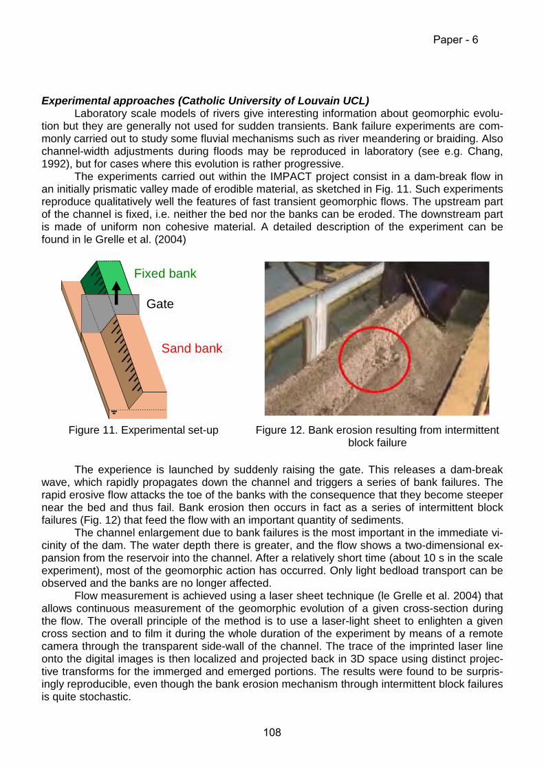
Experimental approaches (Catholic University of Louvain UCL)Laboratory scale models of rivers give interesting information about geomorphic evolu-

tion but they are generally not used for sudden transients. Bank failure experiments are com-monly carried out to study some fluvial mechanisms such as river meandering or braiding. Alsochannel-width adjustments during floods may be reproduced in laboratory (see e.g. Chang,1992), but for cases where this evolution is rather progressive.

The experiments carried out within the IMPACT project consist in a dam-break flow inan initially prismatic valley made of erodible material, as sketched in Fig. 11. Such experimentsreproduce qualitatively well the features of fast transient geomorphic flows. The upstream partof the channel is fixed, i.e. neither the bed nor the banks can be eroded. The downstream partis made of uniform non cohesive material. A detailed description of the experiment can befound in le Grelle et al. (2004)

Fixed bank

Gate

Sand bank

Figure 11. Experimental set-up Figure 12. Bank erosion resulting from intermittentblock failure

The experience is launched by suddenly raising the gate. This releases a dam-breakwave, which rapidly propagates down the channel and triggers a series of bank failures. Therapid erosive flow attacks the toe of the banks with the consequence that they become steepernear the bed and thus fail. Bank erosion then occurs in fact as a series of intermittent blockfailures (Fig. 12) that feed the flow with an important quantity of sediments.

The channel enlargement due to bank failures is the most important in the immediate vi-cinity of the dam. The water depth there is greater, and the flow shows a two-dimensional ex-pansion from the reservoir into the channel. After a relatively short time (about 10 s in the scaleexperiment), most of the geomorphic action has occurred. Only light bedload transport can beobserved and the banks are no longer affected.

Flow measurement is achieved using a laser sheet technique (le Grelle et al. 2004) thatallows continuous measurement of the geomorphic evolution of a given cross-section duringthe flow. The overall principle of the method is to use a laser-light sheet to enlighten a givencross section and to film it during the whole duration of the experiment by means of a remotecamera through the transparent side-wall of the channel. The trace of the imprinted laser lineonto the digital images is then localized and projected back in 3D space using distinct projec-tive transforms for the immerged and emerged portions. The results were found to be surpris-ingly reproducible, even though the bank erosion mechanism through intermittent block failuresis quite stochastic.

Paper - 6

108

Numerical modeling development (UCL)The key issue in modeling geomorphic processes is to properly include bank failure

mechanisms in the system. Indeed, such important geomorphic changes occur randomly andabruptly, and cannot be considered just as a continuous process such as bedload transport.Two different models were developed by UCL within the frame of the IMPACT project.

First, a 2D extension of the model presented for the near field (Eq. 4-5) was developed,including a bank erosion mechanism. A detailed description of the method, summarized here,can be found in Spinewine et al. (2002) and Capart and Young (2002). The key idea is that byallowing separate water and fluid-like slurry layers to flow independently, the governing equa-tions are fully equipped to deal with flow slides of bank material slumping into the waterstream. Once failure is initiated, the post-failure flow can be captured just like any other patternof water and sediment motion.

A liquefaction criterion is needed to determine when and where portions of the banksare to be transformed from a solid-like to a fluid-like medium. Therefore, the following funda-mental mechanism is assumed: activation of a block failure event occurs whenever and wher-ever the local slope exceeds a critical angle ϕc. An extended failure surface is then defined asa cone centered on the failure location and sloping outwards at residual angle ϕr < ϕc. Finally,sediment material above this cone is assumed to instantaneously liquefy upon failure.

In order to account for the observed contrast between submerged and emerged regions,four distinct angles of repose are defined as indicated in Fig. 13: angles ϕcs and ϕrs apply tothe submerged domain, and ϕce and ϕre to the emerged domain.

z z− s0

unstable metastable stable

submergedemergedhw0

( )( ) +( )x x y y− −0 02 2 1/2

Figure 13. Stability diagram for the 2D geostatic failure operator

The second model selected for coupling with the above bank erosion mechanism is aone- dimensional scheme. It comprises a hydrodynamic finite-volume algorithm and a separatesediment transport routine (paper in preparation). The finite-volume scheme, developed withthe aim of coping with complex topographies (Soares-Frazão and Zech, 2002), solves the hy-drodynamic shallow-water equations, under the form of Eq. 13-14.

The changes in cross-sectional geometry due to longitudinal sediment transport (bed-load) over one computational time step are derived from the Exner continuity equation of thesediment phase (Eq. 15).

In addition to sediment fluxes at the upstream and downstream faces of a cell, lateralsediment inflow resulting from bank failures must be considered. A failure is triggered by thesubmergence of a bank by a rise ∆h in water level that destabilises a prismatic portion of mate-rial as sketched in Fig. 14 that results in a lateral solid discharge qs. The final shape of thecross section shows a submerged slope of angle αe,s (angle of repose under the water level

Paper - 6

109

after erosion) while the emerged part gets the angle αe,e corresponding to the angle of reposeof humid sand above the water level after the erosion process.

Figure 14. Bank failure triggered by the sub-mergence of the bank

Figure 15. Deposition of the material erodedfrom the banks

The eroded material deposits into the channel as sketched in Fig. 15. The submergedportion deposits with an angle αd,s corresponding to the angle of repose under water while theemerged portion stabilizes at an angle αd,s (angle of repose above the water level after thedeposition process). All those angles of repose are specific to the material used in the experi-ments and were measured by means of static and dynamic experiments.

Finally, the numerical 1D model consists in solving in a de-coupled way the three differ-ent key steps of the process: (i) the hydrodynamic routing of the water, (ii) the longitudinalsediment transport and the resulting erosion and deposition, and (ii) the bank failures and theresulting morphological changes in the cross-section shape.

Validation of the models (UCL, UT, Cemagref, IST)Validation of the models will be achieved through benchmarking at two different levels.

A first benchmark concerns the idealized dam-break flow experiment presented in a previoussection. The blind test was achieved by the involved partners and the comparison process isunderway. The second level concerns the simulation of a real event, namely the Lake Ha!Ha!flood that occurred in the Saguenay region of Quebec in 1996 (Brooks and Lawrence, 1999).This second benchmark has just started and the blind modeling by the partners is in progress.

Some preliminary comparisons for the first benchmark are presented in Fig. 16. The ex-perimental measurements are compared to the results obtained by the 1D model developed byUCL. The overall agreement is good: the numerical model appears to follow quite accuratelythe progressive enlargement of the cross section.

Conclusions

The problem with dam-break induced geomorphic flows is that they combine severaldifficulties. They involve such rapid changes and intense rates of transport that the granularcomponent plays an active role in the flow dynamics, and that inertia exchanges between thebed and the flow become important. Dam-break induced geomorphic flows generate intenseerosion and solid transport, resulting in dramatic and rapid evolution of the valley geometry. Inreturn, this change in geometry strongly affects the wave behavior and thus the arrival timeand the maximum water level.

Paper - 6

110

(a) (c)

(b) (d)Figure 16. Bank erosion benchmark: comparison between UCL 1D model and experiments

Distance downstream from the dam: 0.50 m (a-b), 1.50 m (c-d) : initial situation, experiments, and numerical modeling

In the near field, rapid and intense erosion accompanies the development of the dam-break wave, leading to an intense transient debris flow. The numerical models existing at thisstage provide encouraging results. The jump at the water surface, the scouring at the dam lo-cation, and the moving layer thickness are fairly well represented. But the earlier stage of thedam-break flow is not so well modeled, since the vertical movements depart from the shallow-water assumptions. Finally, all those phenomena dissipate some energy, what is not repre-sented in the models, what explains that the computed front is generally too fast at the begin-ning.

For the far field behavior, the models at this stage can produce valuable results to com-pare with experimental data from idealized situations, but it is suspected that we are far from acompletely integrated model able to accurately simulate a complex real case. A tentative an-swer to this could probably be given from the results of the second benchmark regarding theLake Ha!Ha! test case, available after the last IMPACT meeting to be held in Zaragoza, Spain,in November 2004.

Acknowledgements

The authors wish to acknowledge the financial support offered by the European Com-mission for the IMPACT project under the fifth framework program (1998-2002), Environmentand Sustainable Development thematic program, for which Karen Fabbri was the EC ProjectOfficer. In addition, the authors acknowledge the financial support offered by the Fonds pour laRecherche dans l’Industrie et l’Agriculture, Belgium and by the Fonds National de la Recher-che Scientifique, Belgium.

Paper - 6

111

References

(1) Armanini A., Fraccarollo L., Guarino L., Martino R., Bin Y . (2000). Experimental analysisof the general features of uniform debris flow over a loose bed. Proceedings Second Int.Conf. on Debris-Flow Hazards Mitigation, Taipei, Taiwan, August 2000, 327-334.

(2) Armanini A., Fabrizi R.B., Fraccarollo L., Giuliani M., Larcher M., Rosatti G. (2003) Dy-namics of steady and unsteady granular debris flows with uniform material. In EC Con-tract EVG1-CT-2001-00037 IMPACT Investigation of Extreme Flood Processes and Un-certainty, Proceedings 3rd Project Workshop, Louvain-la-Neuve, Belgium 6-7 November2003 (CD-ROM).

(3) Brooks G.R, Lawrence D.E. (1999) The drainage of Lake Ha!Ha! reservoir and down-stream geomorphic impacts along Ha!Ha! River, Saguenay area, Quebec, Canada.Geomorphology 28: 141-168.

(4) Benito G., Grodek T., Enzel Y. (1998). The geomorphic and hydrologic impacts of thecatastrophic failure of flood-control dams during the 1996-Biescas flood (Central Pyren-ees, Spain). Z. Geomorph. 42, 417-437.

(5) Capart H., Fraccarollo L., Guarino L., Armanini A., Zech Y. (1999). Recent developmentsin debris-flow characterisation by digital imaging measurements, CD-ROM proceedingsof the 4th CADAM meeting Zaragoza, Spain, 367-380.

(6) Capart H. (2000) Dam-break induced geomorphic flows. PhD thesis, Universitécatholique de Louvain, Louvainla-Neuve, Belgium

(7) Capart H., Young D.L., Zech Y. (2001) Dam-break induced debris flow. “Particulate grav-ity currents”, special publication of the International Association of Sedimentologists (edsB Kneller, B McCaffrey, J Peakall, T Druitt), vol. 31, 2001, pp. 149-156.

(8) Capart H., Young D.L. (2002) Two-layer shallow water computations of torrential geo-morphic flows. Proceedings of River Flow 2002, Louvain-la-Neuve, Belgium, September2002.

(9) Chang H.H. (1992). Fluvial processes in river engineering. Krieger publishing company,Malabar, Florida.

(10) Chapman S., Cowling, T.G. (1970). The Mathematical Theory of Non-Uniform Gases, 3rd

Edn. Cambridge University Press.(11) Costa J.E., Schuster R.L. (1988) The formation and failure of natural dams. Bull. Geol.

Soc. Am. 100: 1054-1068.(12) El Kadi Abderrezzak K. and Paquier A. (2003). IMPACT project: Dam-break waves over

movable beds. In EC Contract EVG1-CT-2001-00037 IMPACT Investigation of ExtremeFlood Processes and Uncertainty, Proceedings 3rd Project Workshop, Louvain-la-Neuve,Belgium 6-7 November 2003 (CD-ROM).

(13) Ferreira R., Leal J., Cardoso A.H. and Almeida A.B. (2003). Sediment Transport by Dam-Break Flows. A Conceptual Framework Drawn from the Theories for Rapid GranularFlows. In EC Contract EVG1-CT-2001-00037 IMPACT Investigation of Extreme FloodProcesses and Uncertainty, Proceedings 3rd Project Workshop, Louvain-la-Neuve, Bel-gium 6-7 November 2003 (CD-ROM).

(14) Fraccarollo L., Capart H. (2002). Riemann wave description of erosional dam-breakflows. Journal of Fluid Mechanics, 461, 183-228.

(15) Fraccarollo L., Capart H., Zech Y. (2003). A Godunov method for the computation of ero-sional shallow water transient. Int. Journal of Numerical Methods in Fluids, 41:951-976.

Paper - 6

112

(16) Gallino G.L., Pierson T.C. (1985). Pollalie Creek debris flow and subsequent dam-breakflood of 1980, East Fork Hood River Basin, Oregon. U. S. Geological Survey Water Sup-ply Paper 2273, 22 pages.

(17) Iverson R.M. (1997). The physics of debris flow. Reviews of Geophysics, 35, 3, 245-296.(18) Jenkins J.T., Hanes D.M. (1998). Collisional sheet flows of sediment driven by a turbulent

fluid. Fluid Mechanics, vol. 370: 29-52, Cambridge University Press.(19) Kale V.S., Ely L.L., Enzel Y., Baker V.R. (1994). Geomorphic and hydrologic aspects of

mon-soon floods on the Narmada and Tapi Rivers in central India. Geomorphology 10,157-168.

(20) Leal J.G.A.B., Ferreira R.M.L., Cardoso A.H., Almeida A.B. (2003). Overview of ISTGroup Results on the Sediment Benchmark. In EC Contract EVG1-CT-2001-00037IMPACT Investigation of Extreme Flood Processes and Uncertainty, Proceedings 3rdProject Workshop, Louvain-la-Neuve, Belgium 6-7 November 2003 (CD-ROM).

(21) le Grelle N., Spinewine B., Soares-Frazão S., Zech Y. (2004). Non-intrusive imagingmeasurements of the morphological evolution of a channel during a dam-break flow. Pro-ceedings of River Flow 2004, Naples, Italy, June 2004

(22) Ogawa S. (1978). Multitemperature Theory of Granular Materials. Proc. U.S-JapanSeminar on Continuum Mechanical and Statistical Approaches in the Mechanics ofGranular Materials, S. C. Cowin & M. Satake Eds., Gakujutsu Bunken Fukyukai, Tokyo,208-217.

(23) Soares-Frazão S., Zech Y. (2002) Dam-break in channels with 90° bend, Journal of Hy-draulic Engineering, American Society of Civil Engineers (ASCE), Vol. 128, n°11, pp.956-968

(24) Spinewine B., Capart H., Le Grelle N., Soares-Frazão S., Zech Y (2002). Experimentsand computations of bankline retreat due to geomorphic dam-break floods. Proceedingsof River Flow 2002, Louvain-la-Neuve, Belgium, September 2002

(25) Spinewine B., Zech Y. (2002a). Geomorphic dam-break floods: near-field and far-fieldperspectives. In EC Contract EVG1-CT-2001-00037 IMPACT Investigation of ExtremeFlood Processes and Uncertainty, Proceedings 1st Project Workshop, Wallingford, UK,16-17 May 2002 (CD-ROM).

(26) Spinewine B., Zech Y. (2002b) Dam-break waves over movable beds: a “flat bed” testcase. In EC Contract EVG1-CT-2001-00037 IMPACT Investigation of Extreme FloodProcesses and Uncertainty, Proceedings 2nd Project Workshop, Mo-i-Rana, Norway, 12-13 September 2002 (CD-ROM).

(27) Spinewine B. (2003). Ecoulements transitoires sévères d’un milieu diphasique liquide /granulaire (eau / sédiments), en tenant compte du couplage rhéologique entre les deuxphases et des composantes verticales du mouvement (in French). MSc thesis. Universitécatholique de Louvain, Louvain-la-Neuve, Belgium

(28) Spinewine B., Capart H., Larcher M., Zech Y. (2003). Three-dimensional Voronoï imag-ing methods for the measurement of near-wall particulate flows. Experiments in Fluids,vol. 34, pp. 227-241

(29) Toro E.F. (1997) Riemann Solvers and Numerical Methods for Fluid Dynamics. A Practi-cal Introduction. Springer-Verlag, Berlin, Germany

(30) Zech Y., Spinewine B. (2002). Dam-break induced floods and sediment movement –State of the art and need for research. In EC Contract EVG1-CT-2001-00037 IMPACTInvestigation of Extreme Flood Processes and Uncertainty, Proceedings 1st ProjectWorkshop, Wallingford, UK, 16-17 May 2002 (CD-ROM).

Paper - 6

113

PROCESS UNCERTAINTY:ASSESSING AND COMBINING UNCERTAINTY BETWEEN MODELS

Mark Morris, HR Wallingford UKMohamed Hassan, HR Wallingford UK

Francisco Alcrudo, UDZ, SpainYves Zech, UCL, Belgium

Karim Lakhal, Engineering School of Science and Technology of Lyon France

Abstract

The uncertainty associated with breach formation, flood propagation, and sedimentmovement is important in the risk management of these structures. Assessing risks involvesidentifying the hazards associated with each issue. This paper identifies the advances thathave been made as a result of the IMPACT Project research. Guidance and relativeimportance of the uncertainty for each process is considered for the purposes of improved riskmanagement of these structures.

Scoping the Problem

The wider pictureUncertainty is a general concept that reflects our lack of sureness about something,

ranging from just short of complete sureness to an almost lack of conviction about an outcome!Two main sources of uncertainty include:

1. Natural variability: referring to the randomness observed in nature.2. Knowledge uncertainty: referring to our state of knowledge of a system and our ability to

measure and model it.

Knowledge uncertainty may be further divided according to:1. Statistical uncertainty: referring to the uncertainty resulting from the need to extrapolate

a particular set of data.2. Process model uncertainty: describing the uncertainty associated with using a process

model based on incomplete knowledge of the process, data, or representation of reality.3. Decision uncertainty: describing the strength of belief in the decision made and its

robustness. This decision is likely to be linked to one or all of the above categories ofuncertainty.

Work on uncertainty1 within the IMPACT2 project focuses on knowledge uncertainty –and specifically process model uncertainty.

1 It should be noted that the word uncertainty means process model uncertainty for numerical models for the rest of this document.

2 IMPACT Project: Investigation of Extreme Flood Processes and Uncertainty. EC Contract No: EVG1-CT-2001-00037. www.impact-project.net

Paper - 7

114

Scope of work feasible within the IMPACT ProjectThe objective of this work package is to identify and emphasise the uncertainty

associated with the various components of the flood prediction process; namely breachformation, flood routing and sediment transport. The effect that uncertainty in each of thesepredictions has on the overall flood prediction process will be demonstrated through applicationto a real or virtual case study. Thus, the focus of work under IMPACT was to:

a) Investigate uncertainty within modelling predictions for predicting breachformation, flood propagation and sediment transport

b) Demonstrate how uncertainty within each of these modelling approaches maycontribute towards overall uncertainty within the prediction of specific conditions(such as flood water level at a specific location)

c) Consider the implications of uncertainty in specific flood conditions (such aswater level, time of flood arrival etc.) for end users of the information (such asemergency planners).

The scope of work under IMPACT does not allow for an investigation of uncertainty inthe impact of flooding or in the assessment and management of flood risk. The assessment ofmodelling uncertainty provides essential information upon which a later assessment of theuncertainty in risk may be developed through further research.

The IMPACT Approach

The challenge of assessing overall modelling uncertainty is complicated by the need toassess uncertainty within two or more models, to somehow transfer a measure of uncertaintybetween these models and to develop a system that allows for the different complexities of thevarious models. Two basic approaches were adopted, namely sensitivity analysis and MonteCarlo analysis. However, whilst a breach formation model may be able to run hundreds orthousands of simulations within a period of hours, it is unrealistic to assume that a complex 2Dflood propagation model can undertake a similar process without undertaking weeks or monthsof analysis. A compromise solution was adopted for IMPACT that combines sensitivityanalysis, Monte Carlo simulation and expert judgement. Whilst this approach may provide anestimate of uncertainty which contains a degree of subjectivity (expert judgement) it alsoprovides a mechanism that is achieved relatively simply and provides a quick indication ofpotential uncertainty.

Sensitivity AnalysesThe uncertainty of various modelling parameters is examined here by first selecting

some representative values for each parameter (e.g. the upper, most likely, and lower values).The modeller then runs the model using these values for each parameter. The output from themodel for values other than the most likely value can then be compared with the output of themost likely value or a range is assigned to this model output in relation with the range of theinput parameter. This comparison gives an indication of the uncertainty in output derived fromeach of the input parameters.

For example, consider the situation whereby the broad crested weir equation is used ina numerical model and an assessment of the uncertainty contributed by the weir coefficient

Paper - 7

115

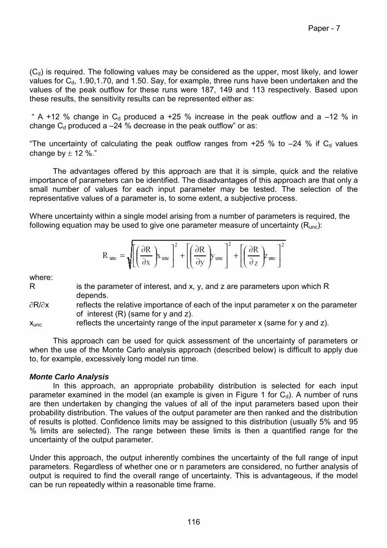
(Cd) is required. The following values may be considered as the upper, most likely, and lowervalues for Cd, 1.90,1.70, and 1.50. Say, for example, three runs have been undertaken and thevalues of the peak outflow for these runs were 187, 149 and 113 respectively. Based uponthese results, the sensitivity results can be represented either as:

“ A +12 % change in Cd produced a +25 % increase in the peak outflow and a –12 % inchange Cd produced a –24 % decrease in the peak outflow” or as:

“The uncertainty of calculating the peak outflow ranges from +25 % to –24 % if Cd valueschange by ± 12 %.”

The advantages offered by this approach are that it is simple, quick and the relativeimportance of parameters can be identified. The disadvantages of this approach are that only asmall number of values for each input parameter may be tested. The selection of therepresentative values of a parameter is, to some extent, a subjective process.

Where uncertainty within a single model arising from a number of parameters is required, thefollowing equation may be used to give one parameter measure of uncertainty (Runc):

where:R is the parameter of interest, and x, y, and z are parameters upon which R

depends.∂R/∂x reflects the relative importance of each of the input parameter x on the parameter

of interest (R) (same for y and z).xunc reflects the uncertainty range of the input parameter x (same for y and z).

This approach can be used for quick assessment of the uncertainty of parameters orwhen the use of the Monte Carlo analysis approach (described below) is difficult to apply dueto, for example, excessively long model run time.

Monte Carlo AnalysisIn this approach, an appropriate probability distribution is selected for each input

parameter examined in the model (an example is given in Figure 1 for Cd). A number of runsare then undertaken by changing the values of all of the input parameters based upon theirprobability distribution. The values of the output parameter are then ranked and the distributionof results is plotted. Confidence limits may be assigned to this distribution (usually 5% and 95% limits are selected). The range between these limits is then a quantified range for theuncertainty of the output parameter.

Under this approach, the output inherently combines the uncertainty of the full range of inputparameters. Regardless of whether one or n parameters are considered, no further analysis ofoutput is required to find the overall range of uncertainty. This is advantageous, if the modelcan be run repeatedly within a reasonable time frame.

Paper - 7

116

0

1

2

3

4

5

6

1.4 1.5 1.6 1.7 1.8 1.9 2

Cd

Like

lihoo

d

Figure 1: Example triangular probability distribution of Cd

Figure 2 shows an example of this approach where 1000 runs were undertaken, leading to thedistribution shown. Taking the confidence limits as 5% and 95%, the range of uncertaintywould be 55-180 m3/s with a likely peak outflow of 120 m3/s (at 50%). This translates to – 65m3/s to + 60 m3/s uncertainty in the peak outflow generated from all of the selected inputparameters.

02 04 06 08 0

1 0 01 2 01 4 01 6 01 8 02 0 0

0 20 40 60 80 100

120

140

160

180

200

220

240

260

280

300

Mor

e

P e a k o u tflo w ra n k s

Freq

uenc

y

Figure 2: Peak outflow distribution based on the Monte Carlo analysis approach

The advantages of this approach are that a wider range of data is tested giving a betterindication of uncertainty in comparison to a simple sensitivity analysis. In addition, a probabilitydistribution is produced for the output parameters (e.g. Peak outflow). The main disadvantagesof this approach are that the relative importance of each input parameter is not identified and agreater number of model runs is required in comparison to the simple sensitivity analysisapproach (i.e. long run time).

Paper - 7

117

Balancing the ApproachWith the pros and cons of each approach in mind, the approach adopted by IMPACT

was to:

1 Assess breach model uncertainty via sensitivity analysis and Monte Carlo simulation2 Extract representative flood hydrographs from the breach model analyses representing

upper, mid and lower scenarios for use in flood propagation3 Assess flood propagation models through sensitivity analysis only4 Either select flood propagation model parameters to match upper, mid and lower

scenarios for running with upper, mid and lower scenario breach hydrographs – endingwith three sets of model predictions

orSelect upper, mid and lower scenario parameters for application to each of the 3 breachhydrographs, resulting in 9 sets of model predictions, from which representative upper,mid and lower conditions may be extracted (see Figure 3)

Figure 3: Linking uncertainty analysis between models

Example Analysis of Uncertainty within a Breach Model

The HR BREACH model has been used to develop and demonstrate the approach foruncertainty analysis. Data from the Norwegian Field Test #2 (homogeneous non-cohesivefield), which was undertaken in Norway in 2002, was selected for analysis. This field test(Figure 4) was built mainly from non-cohesive materials (D50 ≈ 5 mm) with less than 5 % fines.The purpose of this test was to better understand breach formation and to identify the differentfailure mechanisms in homogeneous non-cohesive embankments failed by overtopping. Moreinformation on the field test programme may be found in Vaskinn (2004). Hassan (2002) givesan overview of the HR BREACH model whilst Morris(2005) gives an overall report on theIMPACT project.

Paper - 7

118

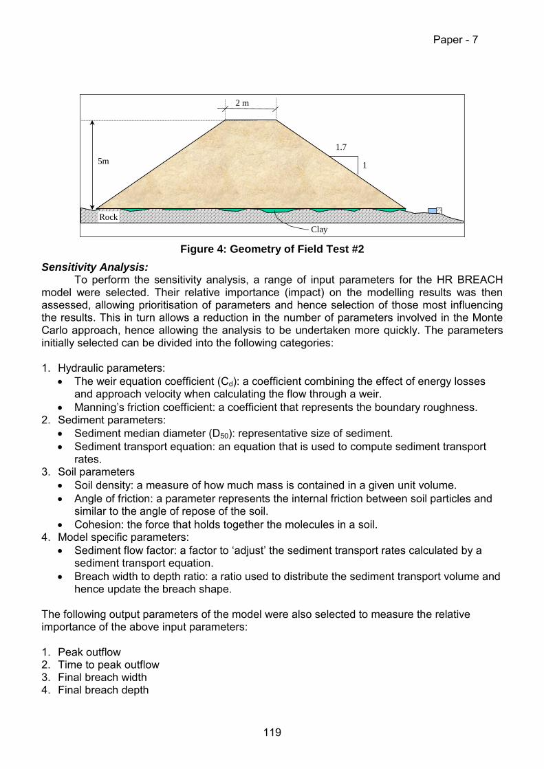
2 m

1.7

15m

ClayRock

Figure 4: Geometry of Field Test #2Sensitivity Analysis:

To perform the sensitivity analysis, a range of input parameters for the HR BREACHmodel were selected. Their relative importance (impact) on the modelling results was thenassessed, allowing prioritisation of parameters and hence selection of those most influencingthe results. This in turn allows a reduction in the number of parameters involved in the MonteCarlo approach, hence allowing the analysis to be undertaken more quickly. The parametersinitially selected can be divided into the following categories:

1. Hydraulic parameters:• The weir equation coefficient (Cd): a coefficient combining the effect of energy losses

and approach velocity when calculating the flow through a weir.• Manning’s friction coefficient: a coefficient that represents the boundary roughness.

2. Sediment parameters:• Sediment median diameter (D50): representative size of sediment.• Sediment transport equation: an equation that is used to compute sediment transport

rates.3. Soil parameters

• Soil density: a measure of how much mass is contained in a given unit volume.• Angle of friction: a parameter represents the internal friction between soil particles and

similar to the angle of repose of the soil.• Cohesion: the force that holds together the molecules in a soil.

4. Model specific parameters:• Sediment flow factor: a factor to ‘adjust’ the sediment transport rates calculated by a

sediment transport equation.• Breach width to depth ratio: a ratio used to distribute the sediment transport volume and

hence update the breach shape.

The following output parameters of the model were also selected to measure the relativeimportance of the above input parameters:

1. Peak outflow2. Time to peak outflow3. Final breach width4. Final breach depth

Paper - 7

119

Table 1 below shows the base values used in the model to simulate the failure of thetest case. These values were considered the ‘base’ for comparison as they represent thebest estimate value for each parameter and they are either measured in the field,estimated, or default values of the model. Table 1 also shows the range values that wereselected for each parameter to undertake the sensitivity analysis. This range of values waseither based upon the variation of the measured data (e.g. D50) or judgement of what is areasonable range for each parameter (i.e. Cd). 5 variations of each parameter wereconsidered enough to present the valid range for this test case except for the sedimenttransport equation where only the three available equations in the model were used varyingthe sediment flow factor once. Therefore, 44 model runs were undertaken, in addition to thebase run, varying only one parameter for each run and recording its effect on the selectedoutput parameters.

Table 1: Base value and variations of each parameterVariationsInput

ParametersBaseValue 1 2 3 4 5

CD 1.50 1.55 1.60 1.70 1.80 1.90Mannings’n 0.020 0.025 0.030 0.035 0.040 0.045D50 (mm) 4.65 2.00 3.00 4.00 5.00 6.00Density(KN/m3)

21.15 19.00 20.00 21.00 22.00 23.00

Angle ofFriction (o)

42 25 30 35 40 45

Sediment flowfactor

1.0 0.5 1.5 2.0 2.5 3.0

Breach width todepth ratio

0.50 1.00 1.50 1.75 2.00 2.50

Sedimenttransportequation

Yang Visser (1flow factor)

Chen(Sand) (1

flow factor)

Visser (2flow factor)

Chen(Sand) (2

flow factor)

---

Cohesion(KN/m2)

0.9 0.0 2.0 2.0 7.0 10.0

As an example of the output of the sensitivity analysis, Table 2 shows the minimum,maximum, and mean values of the peak outflow (obtained by varying the input parameters)and also the outcome of the base run for those parameters. It also shows the minimum,maximum, and the range of variation from the mean and the base values. Based upon thesensitivity analysis results, It was found that:

1- The sediment transport equation and the sediment flow factor are consistently showing thehighest impact on all output parameters.

2- The angle of friction, however to a less extent than the two parameters above, is constantlyshowing a higher impact than other physical parameters.

3- Other physical parameters such as D50, Manning‘s n, and Cd and model parameters suchas the breach width to depth ratio have a lesser effect than the above input parameters.

4- Cohesion has a low effect on the model output parameters. This is expected for a non-cohesive embankment where the value of cohesion is very low.

Paper - 7

120

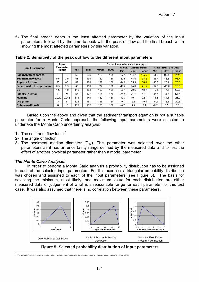
5- The final breach depth is the least affected parameter by the variation of the inputparameters, followed by, the time to peak with the peak outflow and the final breach widthshowing the most affected parameters by this variation.

Table 2: Sensitivity of the peak outflow to the different input parameters

Based upon the above and given that the sediment transport equation is not a suitableparameter for a Monte Carlo approach, the following input parameters were selected toundertake the Monte Carlo uncertainty analysis:

1- The sediment flow factor3

2- The angle of friction3- The sediment median diameter (D50). This parameter was selected over the other

parameters as it has an uncertainty range defined by the measured data and to test theeffect of another physical parameter rather than a model parameter.

The Monte Carlo Analysis:In order to perform a Monte Carlo analysis a probability distribution has to be assigned

to each of the selected input parameters. For this exercise, a triangular probability distributionwas chosen and assigned to each of the input parameters (see Figure 5). The basis forselecting the minimum, most likely, and maximum value for each distribution are eithermeasured data or judgement of what is a reasonable range for each parameter for this testcase. It was also assumed that there is no correlation between these parameters.

Sediment Flow Factor Probability Distribution

D50 Probability Distribution Angle of Friction Probability Distribution

0

0.1

0.2

0.3

0.4

0.5

0.6

2 4 6D50 Value

Like

lihoo

d

0

0.02

0.04

0.06

0.08

0.1

0.12

25 30 35 40 45Angle of Friction Value

Like

lihoo

d

0

0.2

0.4

0.6

0.8

1

0.5 1 1.5 2 2.5 3Sediment Flow Factor Value

Like

lihoo

d

Figure 5: Selected probability distribution of input parameters 3 The sediment flow factor relates to the distribution of sediment movement around the wetted perimeter of the breach formation area (Mohamed (2002)).

Paper - 7

121

The question now arises as to how many runs should be undertaken to ensure that theresults truly reflect the full range of possibilities. It was considered that 30-50 runs are neededfor each parameter. This means that for 3 parameters a total number of (30)3 to (50)3 runs arerequired, which = 27000 – 125000 runs! This number of runs is clearly impractical in terms oftime and effort. Reducing the number of runs from range from 30-50 per parameter to say 10per parameter (tactical Monte Carlo) = 1000 runs, which is achievable. The adequacy of thisnumber of runs can be checked by considering how the probability distribution of the outputparameters is converging towards a consistent distribution with the number of runs.

Figure 6 shows the probability distribution of the model peak outflows after undertaking theMonte Carlo analysis.

0-65

70-7

5

80-8

5

90-9

5

100-

105

110-

115

120-

125

130-

135

140-

145

150-

155

160-

165

170-

175

180-

185

190-

195

200-

205

210-

215

220-

225

230-

235

240-

245

250-

255

260-

265

270-

275

280-

285

290-

295

New0.00

10.00

20.00

30.00

40.00

50.00

60.00

Freq

uenc

y

Peak outflow ranks (m^3/s)

Peak outflow

5% 50% 95%

Figure 6: Probability distribution of peak outflow

The following conclusions were drawn from the results of the Monte Carlo analysis for this testcase:

1- The probability distribution of each output parameter has converged towards a consistentdistribution for all parameters.

2- The final breach depth is the least affected parameter by the variation of the model-inputparameters.

3- The range of variation of the model output parameters is very similar to that obtained for thesame parameters using the sensitivity analysis.

4- The probability distribution of all the monitored output parameters except the final breachdepth converged to approximately a triangular distribution.

Paper - 7

122

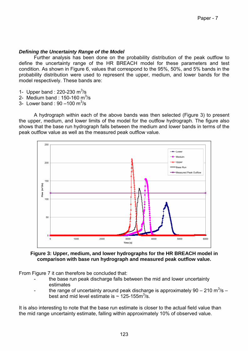
Defining the Uncertainty Range of the ModelFurther analysis has been done on the probability distribution of the peak outflow to

define the uncertainty range of the HR BREACH model for these parameters and testcondition. As shown in Figure 6, values that correspond to the 95%, 50%, and 5% bands in theprobability distribution were used to represent the upper, medium, and lower bands for themodel respectively. These bands are:

1- Upper band : 220-230 m3/s2- Medium band : 150-160 m3/s3- Lower band : 90 –100 m3/s

A hydrograph within each of the above bands was then selected (Figure 3) to presentthe upper, medium, and lower limits of the model for the outflow hydrograph. The figure alsoshows that the base run hydrograph falls between the medium and lower bands in terms of thepeak outflow value as well as the measured peak outflow value.

0

50

100

150

200

250

0 1000 2000 3000 4000 5000 6000Time (s)

Flow

(m

^3/s

)

Lower

Meduim

Upper

Base Run

Measured Peak Outflow

Figure 3: Upper, medium, and lower hydrographs for the HR BREACH model incomparison with base run hydrograph and measured peak outflow value.

From Figure 7 it can therefore be concluded that:- the base run peak discharge falls between the mid and lower uncertainty

estimates- the range of uncertainty around peak discharge is approximately 90 – 210 m3/s –

best and mid level estimate is ~ 125-155m3/s.

It is also interesting to note that the base run estimate is closer to the actual field value thanthe mid range uncertainty estimate, falling within approximately 10% of observed value.

Paper - 7

123

Analysis of Uncertainty within Flood Propagation and Sediment Transport Models

As highlighted earlier, the analysis of uncertainty within flood propagation and sedimenttransport models is not so simple. Within IMPACT, the analysis of uncertainty for the TousDambreak case study will be undertaken for both breach and flood propagation models todemonstrate application of the whole approach. However, this work is scheduled forcompletion during summer 2004 and hence cannot be reported here. Instead, the following twosections provide a short discussion of the issues relating to the prediction of uncertaintyrelating to flood propagation and sediment movement.

Analysis of Uncertainty within Flood Propagation ModelsUncertainty in flood propagation model results is a key issue because many important

decisions depend upon the output of a flood propagation model: Risk maps, land use,evacuation time... depend heavily on the model flood forecast. Within flood propagation modelsthe following sources of uncertainty can be listed:

- Lack of knowledge as regards proper mathematical description of the flood. In fact it iscertain that the mathematical models used (flat pond models, kinematic, dynamic,liberalised or non-linear shallow water models etc…) are not a good enoughmathematical description of a flood. The extent to which one particular model deviatesfrom reality is unknown a priori since some of the conditions that make it fail oftendepend upon the event itself. Unfortunately not much can be done in this respect.

- Lack of knowledge concerning the description of the initial (for instance floodhydrograph) or boundary conditions. Among the latter the bathymetric description of theflooded area can be included, and is usually of paramount importance. However, withcurrent topographic techniques (e.g. LIDAR) this is just a question of economics.

- Uncertainties regarding physical parameters affecting the flood. The most typical is thebottom roughness and its distribution.

Since flood propagation models combine a range of modelling parameters and formulaeit is not a simple process to analyse and understand the effect that one (or more) inputparameters could have on results under a variety of different conditions. The only way to obtainthis relationship is by running the model with different values of every input parameter and toobserve the effect on the outputs (i.e. Monte Carlo type analysis). However, for floodpropagation models the problem is aggravated by the fact that state of the art propagationmodels usually require considerable computing power and can take hours or days to completeone simulation. These constraints typically prevent a Monte Carlo approach and encouragesimpler sensitivity analyses to be undertaken instead.

In the course of the IMPACT project, several attempts to determine the uncertainty offlood propagation models have been carried out depending upon the phase of the project.During model validation against laboratory data, many of the parameters that usually bear acertain amount of uncertainty are relatively well known. This is, for instance, the case with theManning’s n or the topography that is described with high accuracy. Also, most of thecharacteristics of the flood are well controlled during the experiment, and usually subject torepeatability checks: Inflow hydrographs, timing, depth measurements etc… are known withgreat accuracy. Therefore the uncertainty analysis can concentrate on model parameters:Mesh influence, model numerical parameters and strategies have been tested.

Paper - 7

124

When coping with a real case situation some input data are not well known. This is thecase when attempting to model a case study for which the inflow hydrograph is not certain andthe bathymetry prior to the event is not exactly known.

The strategy adopted to ascertain the influence of the inflow hydrograph on the floodcharacteristics and effects downstream entails making several runs of the flood propagationmodel with input hydrographs coming from the uncertainty analysis performed during breachformation work. A representative high, medium and low hydrograph as estimated from thebreach models will be fed to the different flood propagation models. Water elevation at differentlocations will be monitored as a representative output variable to assess the influence of theinflow hydrograph.

Despite the simplicity of the procedure, it is expected that it will provide a measure ofthe uncertainty associated with a representative input parameter.

Analysis of Uncertainty within Sediment Movement Models

IssuesFloods from dam or dike failures induce severe soil movements in various forms. Other

natural hazards also induce such phenomena: glacial-lake outburst floods and landslidesresulting in an impulse wave in the dam reservoir or in the formation of natural dams subject tomajor failure risk. In some cases, the volume of entrained material can reach the same order ofmagnitude (up to millions of cubic meters) as the initial volume of water released from thefailed dam. The risks associated to the sediment movement is thus substantial.

Dam-break induced geomorphic flows generate intense erosion and solid transport,resulting in dramatic and rapid evolution of the valley geometry. In counterpart, this change ingeometry strongly affects the wave behaviour, and thus the arrival time and the maximumwater level, which are the main characteristics to evaluate for risk assessment and alertorganisation. That means that the uncertainties affecting the sediment movement predictionmay critically affect the whole prediction process.

Uncertainties in the sediment movement modellingIn the near field, rapid and intense erosion accompanies the development of the dam-

break wave. Wave breaking occurs at the centre (near the location of the dam), and a nearlyvertical wall of water and debris overruns the sediment bed at the wave forefront, resulting inan intense transient debris flow. Behind the debris-flow front, the behaviour is different: inertialeffects and bulking of the sediments may play a significant role.

Most of the processes involved in this kind of phenomenon are uncertain. The modelsare based on an idealisation of the dam break. The problem is represented in a vertical planeand the dam is supposed to instantaneously disappear without lateral effects. Only the valley-bed material is taken into account in the near-field solid transport, neglecting the materialissued of the breaching itself. At the current stage of the models, the bed mobilisationmodelling is not yet coupled with the breaching modelling. The models are promising foridealised situations but are still far to represent the real-life situations.

Paper - 7

125

Also the data needed for such a modelling are commonly difficult to get. The materialconstituting the reservoir bottom is not uniform, its thickness is not well known, this materialseriously evolves with the time, above all in case of fine material. The material of the valley beddownstream from the dam is also heterogeneous: it consists of soils and rocks in anunpredictable arrangement. Measurement of this is tedious, difficult and expensive.

For the far field, the point is to represent the valley evolution, with a succession oferosion and deposition supplied by the upstream solid transport and by the bank collapses. Apart of the morphologic evolution may be modelled, above all locally, but for a reach of a fewkilometres, there are so many stochastic phenomena involved that the cascade of eventsbecomes unpredictable, forming a kind of uncertainty tree that is difficult to manage.

Overall Progress and Conclusions

A methodology has been developed combining sensitivity analysis, Monte Carloanalysis and expert judgement to allow assessment of modelling uncertainty and integration ofuncertainty between different models. The approach adopted does not adopt a rigorousanalysis of uncertainty, but includes subjective components as a trade off against developing amethod that is practicable given modelling and user time constraints.

The methodology has been applied to the HR BREACH model, using real field data todemonstrate a potential range in breach flood hydrograph results. Similar modelling for theflood propagation of these hydrographs has not yet been completed, but will be undertakenduring summer 2004. The procedure will be demonstrated using the Tous Dam failure as acase study. The analysis will be extended from the dam downstream to the prediction of floodwater levels at selected locations in a town some kilometres below the dam. Based upon therange of uncertainty predicted, implications may then be drawn for the use of such data by endusers such as emergency planners.

Analysis of uncertainty within the field of sediment movement is far less developed. Theissues discussed above all suggest that our ability to model such phenomena is not yet matureenough to allow analysis in detail regarding the uncertainties. It is possible to carry out somesensitivity analyses in order to identify the most relevant among the uncertainty sources.However, the order of magnitude of these uncertainties is still too large to be of immediatevalue and application for end users. It may be concluded therefore that further detailed andfundamental research on this important topic is still needed.

Future Direction of Work

The analysis of uncertainty within dambreak or extreme flood predictions is clearlyimportant if we are to adopt a risk based approach to flood risk management – includingactivities such as emergency planning, land use planning, defence optimisation etc. The scopeof work within the IMPACT project was limited to an assessment of the issues and applicationof relatively simple techniques for assessing potential uncertainty. Clearly, there are multipleaspects to the assessment of uncertainty within the flood risk management concept, thatrequire detailed and fundamental research work. One project where this issue will beconsidered in some considerable detail is the EC FLOODsite project (see www.floodsite.net )

Paper - 7

126

which will run from March 2004 until February 2009. It is also understood that work currentlybeing reported by the Dam Safety Interest Group (DSIG) should also significantly advanceunderstanding in this area.

Acknowledgements

IMPACT is a research project supported by the European Commission under the FifthFramework Programme and contributing to the implementation of the Generic Activity on“Natural and Technological Hazards” within the Energy, Environment & SustainableDevelopment programme. EC Contract: EVG1-CT-2001-00037. The financial support offeredby DEFRA and the Environment Agency in the UK is also acknowledged.

The IMPACT project team comprises Universität Der Bundeswehr München (Germany),Université Catholique de Louvain (Belgium), CEMAGREF (France), Università di Trento (Italy),Universidad de Zaragoza (Spain), Enel.Hydro (Italy), Sweco (formerly Statkraft Grøner AS)(Norway), Instituto Superior Technico (Portugal), Geo Group (Czech Republic), H-EURAqua(Hungary) and HR Wallingford Ltd (UK).

References

Mohamed, M.A.A., SAMUELS, P.G., MORRIS, M.W. and GHATAORA, G.S. (2002). Improvingthe accuracy of prediction of breach formation through embankment dams and floodembankments - Proc. of the Int. Conf. On Fluvial Hydraulics, Louvain-la-Neuve, Belgium, 3-6Sept. 2002 - River Flow 2002, Bousmar & Zech (editors).

Morris M W (2005). IMPACT Project Final Report. European Commission. FP5 ResearchProgramme. Contract No. EVG1-CT-2001-00037. (Draft under development 2004).

Vaskinn KA, Løvell A, Höeg K, Morris M, Hanson G and Hassan MAA (2004). Physicalmodelling of breach formation: Large scale field tests. Association of State Dam SafetyOfficials: Dam Safety 2004. Phoenix, Arizona Sept 2004.

Paper - 7

127

DETERMINATION OF MATERIAL RATE PARAMETERS FOR HEADCUT MIGRATION OF COMPACTED EARTHEN MATERIALS

By 1Greg Hanson, and 2Kevin Cook

Abstract. The timing and formation process of a dam embankment breach due to flood overtopping can dramatically impact the rate that water is released from a reservoir. This rate of water release directly impacts the hazard to life and property downstream of a breached dam. Therefore, dam embankment erosion and breaching from overtopping events is important to both engineers and planners alike, who must predict impacts on local communities and surrounding areas affected by flooding. Based on observations from overtopping tests the erosion process has been described as a four-stage process. A key erosion feature has been observed to be headcut formation and migration. Therefore, determination of the material parameter for predicting rate of headcut migration is important to modeling embankment erosion. An equation for predicting the material parameter based on results from a flume study is compared to results from embankment overtopping tests. Flume tests were conducted on 2 soil materials and embankment-overtopping tests were conducted on 3 soil materials. The flume tests and overtopping tests were compacted using similar compaction efforts. It was concluded that the headcut migration parameter was primarily dependent on compaction water content. A 4% change in compaction water content caused an order of magnitude change in the headcut migration parameter.

1 Greg Hanson, Research Hydraulic Engineer, USDA-ARS, 1301 N. Western St. Stillwater, OK 74075, Phone (405) 624-4135 ext. 224, Fax (405) 624-4136, e-mail: greg.hanson@ars.usda.gov.

2 Kevin Cook, Civil Engineer, USDA-NRCS, State Office, Stillwater, OK 74075, Phone (405) 742-1257 e-mail: Kevin.Cook@ok.usda.gov.

Paper - 8

128

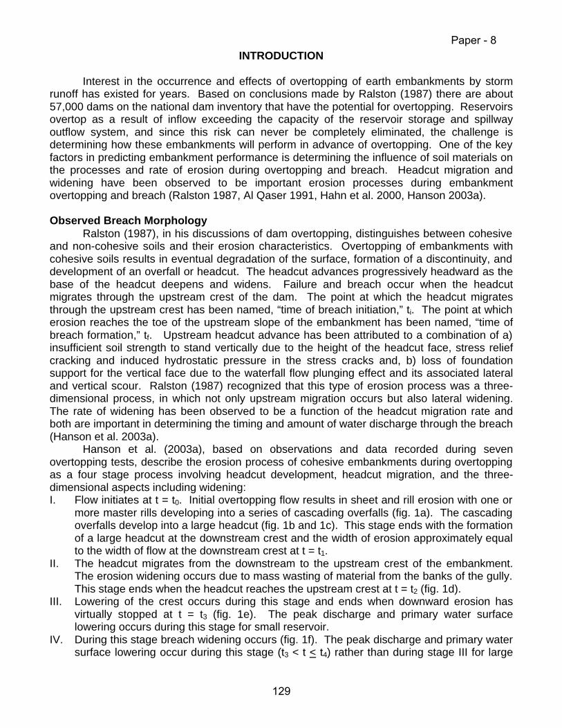
INTRODUCTION

Interest in the occurrence and effects of overtopping of earth embankments by storm runoff has existed for years. Based on conclusions made by Ralston (1987) there are about 57,000 dams on the national dam inventory that have the potential for overtopping. Reservoirs overtop as a result of inflow exceeding the capacity of the reservoir storage and spillway outflow system, and since this risk can never be completely eliminated, the challenge is determining how these embankments will perform in advance of overtopping. One of the key factors in predicting embankment performance is determining the influence of soil materials on the processes and rate of erosion during overtopping and breach. Headcut migration and widening have been observed to be important erosion processes during embankment overtopping and breach (Ralston 1987, Al Qaser 1991, Hahn et al. 2000, Hanson 2003a).

Observed Breach Morphology

Ralston (1987), in his discussions of dam overtopping, distinguishes between cohesive and non-cohesive soils and their erosion characteristics. Overtopping of embankments with cohesive soils results in eventual degradation of the surface, formation of a discontinuity, and development of an overfall or headcut. The headcut advances progressively headward as the base of the headcut deepens and widens. Failure and breach occur when the headcut migrates through the upstream crest of the dam. The point at which the headcut migrates through the upstream crest has been named, “time of breach initiation,” ti. The point at which erosion reaches the toe of the upstream slope of the embankment has been named, “time of breach formation,” tf. Upstream headcut advance has been attributed to a combination of a) insufficient soil strength to stand vertically due to the height of the headcut face, stress relief cracking and induced hydrostatic pressure in the stress cracks and, b) loss of foundation support for the vertical face due to the waterfall flow plunging effect and its associated lateral and vertical scour. Ralston (1987) recognized that this type of erosion process was a three-dimensional process, in which not only upstream migration occurs but also lateral widening. The rate of widening has been observed to be a function of the headcut migration rate and both are important in determining the timing and amount of water discharge through the breach (Hanson et al. 2003a).

Hanson et al. (2003a), based on observations and data recorded during seven overtopping tests, describe the erosion process of cohesive embankments during overtopping as a four stage process involving headcut development, headcut migration, and the three-dimensional aspects including widening: I. Flow initiates at t = t0. Initial overtopping flow results in sheet and rill erosion with one or

more master rills developing into a series of cascading overfalls (fig. 1a). The cascading overfalls develop into a large headcut (fig. 1b and 1c). This stage ends with the formation of a large headcut at the downstream crest and the width of erosion approximately equal to the width of flow at the downstream crest at t = t1.

II. The headcut migrates from the downstream to the upstream crest of the embankment. The erosion widening occurs due to mass wasting of material from the banks of the gully. This stage ends when the headcut reaches the upstream crest at t = t2 (fig. 1d).

III. Lowering of the crest occurs during this stage and ends when downward erosion has virtually stopped at t = t3 (fig. 1e). The peak discharge and primary water surface lowering occurs during this stage for small reservoir.

IV. During this stage breach widening occurs (fig. 1f). The peak discharge and primary water surface lowering occur during this stage (t3 < t < t4) rather than during stage III for large

Paper - 8

129

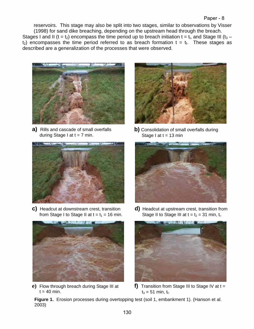
reservoirs. This stage may also be split into two stages, similar to observations by Visser (1998) for sand dike breaching, depending on the upstream head through the breach.

Stages I and II (t = t2) encompass the time period up to breach initiation t = ti, and Stage III (t3 – t2) encompasses the time period referred to as breach formation t = tf. These stages as described are a generalization of the processes that were observed.

a) Rills and cascade of small overfalls during Stage I at t = 7 min.

b) Consolidation of small overfalls during Stage I at t = 13 min

e) Flow through breach during Stage III at t = 40 min.

f) Transition from Stage III to Stage IV at t = t3 = 51 min, tf.

c) Headcut at downstream crest, transition from Stage I to Stage II at t = t1 = 16 min.

d) Headcut at upstream crest, transition from Stage II to Stage III at t = t2 = 31 min, ti.

Figure 1. Erosion processes during overtopping test (soil 1, embankment 1). (Hanson et al. 2003)

Paper - 8

130

Compaction Effects The headcut migration rate is a function of the soil material properties as well as the

hydrodynamic forces and embankment geometry. The embankment materials are typically compacted cohesive soils. It has been observed that the nature and magnitude of compaction have a significant effect on the physical behavior of a soil (White and Gayed 1943, Powledge and Dodge 1985, Robinson and Hanson 1996, Hanson et al. 2003b). White and Gayed (1943) observed from overtopping tests on 0.3 m high embankments constructed in the laboratory that the rate of erosion of the cohesive embankments varied from test to test in such a complicated fashion that the tests could not be correlated numerically. They did observe, however, that the variations could be traced to the clay and water content, to which the erosion rates were very sensitive. Powledge and Dodge (1985) observed that increasing compaction from 95 to 102 percent of standard Proctor compaction resulted in reducing, by half, the erosion of small embankments in flume tests. Robinson and Hanson (1996) conducted large-scale flume studies on headcut migration of cohesive soils. Based on these studies, resistance to headcut migration was reported to increase over several orders of magnitude as compaction water content and compaction energy were increased (Hanson et al. 1998). Hanson et al. (2003b), based on results from seven embankment overtopping tests of 3 different soil materials, observed that since compaction efforts were similar, compaction water content played a major role in setting the rate of erosion of the embankments, including headcut migration and widening. Embankments are constructed of soil material and therefore are affected by these factors in an overtopping event. Therefore it is important to develop algorithms that incorporate hydrodynamic forces as well as soil properties in predicting the erosion processes occurring in an embankment failure during overtopping.

Headcut Migration Prediction

Predicting the rate of headcut migration has been observed to be one of the keys to predicting cohesive embankment failure during overtopping (Hanson et al. 2003a). Simple relationships for headcut migration prediction have almost universally focused on energy at the overfall as the driving mechanism (De Ploey, 1989, Temple 1992, Temple and Moore, 1997). One of the exceptions to the energy-based approach has been a stress-based approach proposed by Robinson and Hanson (1994). The energy-based formulations typically use some form of unit discharge q and headcut height H to describe hydraulic attack in terms of energy dissipation at the headcut. Temple (1992) proposed a simple model describing headcut migration dX/dt based on a material dependent coefficient C and a hydraulic attack parameter A such that:

dX/dt = C(A) (1) A = qaHb (2)

where: a and b = exponents.

Temple and Moore (1997) used a value of 1/3 for both exponent values of a and b. At present there is no approach for determining the material dependent coefficient C

other than based on observed migration rates dX/dt, and q and H. The objective of this paper is to develop a relationship for the material dependent coefficient C based on flume results and compare this relationship to embankment overtopping results.

Paper - 8

131

TEST SETUP Flume Tests

Headcut advance tests were performed in a 1.8-m wide and 29-m long flume with 2.4-m high sidewalls (fig. 2). The test section within the flume was constructed by placing soil in horizontal loose layers 0.15 to 0.20 m thick. A 0.86-m wide vibratory padfoot roller was used to compact each layer, and a hand-held pneumatic compactor was used to compact the soil against the flume walls. Compactive effort and water content were varied from test to test. Prior to testing, a near vertical overfall was preformed at the downstream end of the test section. Overfall heights varied from 0.9 m to 1.5 m. The surface of the fill was protected using carpet strips or a soil cement surface layer to minimize surface erosion and emphasize headcut migration. Following placement of soil in the flume and before testing, samples were taken from the downstream end of the placed soil. The dry unit weight γd and water content wc% were determined as an average of the values determined from undisturbed tube samples. Following soil sampling and headcut forming, the outlet basin was filled with water to the desired level, and flow was delivered to the test flume (fig. 3). Even though advance of the headcut was observed to often be in discrete steps due to mass failures of the soil material at the headcut face, the global rate of movement for a set of flow conditions and soil material properties appeared to be uniform. Therefore, advance rates for each test were determined based on linear regression of the observed headcut position versus time (fig 4).

Headcut migration rates of two soils were examined in these flume experiments, Soil E and Soil F (table 1). Standard proctor tests on Soil E exhibited a maximum dry unit weight of 1.90 Mg/m3 at optimum water content of 12% (fig. 5) while Soil F exhibited a maximum dry unit weight of 1.96 Mg/m3 at optimum water content of 10.5%. A total of 46 tests were conducted using Soil E and Soil F, and in 6 test cases of Soil E and one test case of Soil F the compaction effort was similar to the compaction effort used in the embankment overtopping tests. The compaction water contents and dry unit weights for these seven tests are plotted on figure 5.

Figure 2. Schematic of flume set-up (Robinson and Hanson, 1996).

Paper - 8

132

Water Content %

6 8 10 12 14 16 18 20

Dry

uni

t wei

ght (

Mg/

m3 )

1.65

1.70

1.75

1.80

1.85

1.90

1.95

2.00

2.05

2.10

Soil ESoil F

Saturation = 100%

StandardLaboratoryCompaction

Soil E

Soil F

Figure 5. Compaction results for Soil E and Soil F in the laboratory and in the flume.

Figure 3. Headcut migration test in large outdoor flume.

0 1 2 3 4 5 60

1

2

3

4

5

6

Hea

dcu

t M

igra

tio

n (

m)

Time (h)

Ar=0.83 m/h

Figure 4. Typical observed headcut migration during a flume test.

Paper - 8

133

Embankment Overtopping Tests Three large-scale embankments, two at 2.3 m and one at 1.5 m in height were

constructed and tested. Two of the embankments, 2.3 m high (embankment 1) and 1.5 m high (embankment 2), had three test sections, 7.3 m and 4.9 m wide with 2 m and 1.5m trapezoidal notch overflow sections, respectively (fig. 6), and 3H:1V slopes on both the upstream and downstream sides. The three test sections for each embankment had three different soil materials: Soil 1, Soil 2, and Soil 3 (table 1). In order to test each soil material individually, the notches in the other test sections were filled on the upstream end with a soil plug. The height of the embankment at the notch crests was 1.83 m and 1.22 m for the 2.3 m and 1.5 m high embankments, respectively. The third embankment constructed and tested was 2.3 m high (embankment 3) and had a single 12 m test section of Soil 2 with an 8.2 m wide trapezoidal overflow notch. Embankment 3 was constructed and tested in the same location as embankment 1 (fig. 6). The soils were placed in loose lifts 0.15 m thick and compacted with 2 passes with vibration of a vibratory roller, resulting in a compactive effort similar to the seven flume tests previously described.

Soil Parameters Soil E Soil F Soil 1 Soil 2 Soil 3 Gradation % Clay < 0.002 mm % Silt % Sand

25 40 35

13 30 57

4

28 68

6

30 64

26 48 26

Liquid Limit Plastic Limit Plasticity Index

26 9

15

16 13 3

NP

NP

34 17 17

USCS CL SM SM SM CL Standard Compaction Values Maximum Dry Unit Weight (Mg/m3) Optimum Water Content %

1.90 12.0

1.96 10.5

1.84 9.0

1.86 10.5

1.79 14.0

1.7-membankment

2.3-membankment

ReservoirStaff Gage

1.2-mmodifiedParshallFlume(Inflow)

SupplyCanal

1.2-mH Flume(Outflow)

V – notchWeir(Outflow)

ReservoirDrain

Figure 6. Schematic of embankment overtopping facilities.

2 1&3

Table 1. Properties of soils used in flume and embankment tests.

Paper - 8

134

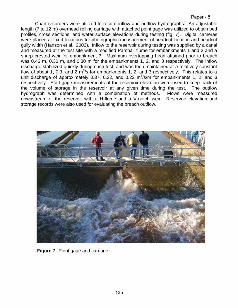
Chart recorders were utilized to record inflow and outflow hydrographs. An adjustable length (7 to 12 m) overhead rolling carriage with attached point gage was utilized to obtain bed profiles, cross sections, and water surface elevations during testing (fig. 7). Digital cameras were placed at fixed locations for photographic measurement of headcut location and headcut gully width (Hanson et al., 2002). Inflow to the reservoir during testing was supplied by a canal and measured at the test site with a modified Parshall flume for embankments 1 and 2 and a sharp crested weir for embankment 3. Maximum overtopping head attained prior to breach was 0.46 m, 0.30 m, and 0.30 m for the embankments 1, 2, and 3 respectively. The inflow discharge stabilized quickly during each test, and was then maintained at a relatively constant flow of about 1, 0.3, and 2 m3/s for embankments 1, 2, and 3 respectively. This relates to a unit discharge of approximately 0.37, 0.22, and 0.22 m3/s/m for embankments 1, 2, and 3 respectively. Staff gage measurements of the reservoir elevation were used to keep track of the volume of storage in the reservoir at any given time during the test. The outflow hydrograph was determined with a combination of methods. Flows were measured downstream of the reservoir with a H-flume and a V-notch weir. Reservoir elevation and storage records were also used for evaluating the breach outflow.

Figure 7. Point gage and carriage.

Paper - 8

135

Table 2. Relevant flume test measurements.

Water Content %

8 9 10 11 12 13 14 15 16 17 18

C (

s-2/3

)

10-5

10-4

10-3

10-2

Soil E Soil F

C = 3000 (wc%)-6.5

Flume Data

Figure 8. Compaction wc% versus C for flume tests at a specific compaction effort.

RESULTS

Flume Tests

The results from the seven flume tests that were compacted with similar compaction effort to the embankment studies indicated that the compaction water content played a significant role in setting the rate of headcut migration (table 2). The migration rate was observed to change 50 times from a compaction water content of 9.2% to 15.9%. The C parameter was calculated from equation 1 using the flume test measurements of q, H, and dX/dt (table 2). A plot of compaction water content wc% versus C (fig. 8) shows the correlation between these two parameters for these seven flume tests. The following equation can be used to estimate C: C = 3000 (wc%)-6.5 (3) where C is in units (s-2/3). Embankment Overtopping Tests

The results from the seven embankment overtopping tests indicate, as did the flume tests, that the compaction water content plays a significant role in influencing the rate of headcut migration (table 3). Stage II of the embankment erosion for the seven tests was used to determine and compare headcut migration rates. Stage II is the phase of erosion in which the headcut that has formed migrates from the downstream crest of the embankment to the upstream crest (Hanson et al. 2003a). This stage was chosen due to the fact that the headcut height is typically equivalent to the embankment height at the notch during this stage, discharge is nearest its constant rate (typically equal to inflow), and the headcut migration rate is nearly constant (fig. 9). Values of C predicted from equation 3 compare well to

Test

#

Soil WC

(%)

γd

(Mg/m3)

dX/dt

(m/s)

q

(m2/s)

H

(m)

C

(s-2/3)

1 E 9.2 1.68 1.5x10-3 0.84 1.2 1.5x10-3

2 F 12.1 1.86 3.5x10-4 0.87 1.2 3.4x10-4

3 E 12.4 1.84 4.1x10-4 0.89 1.2 4.0x10-4

4 E 14.2 1.79 9.3x10-5 0.86 1.3 9.0x10-5

5 E 14.4 1.79 4.2x10-5 0.86 1.3 4.0x10-5

6 E 14.8 1.81 3.5x10-5 1.36 1.0 3.1x10-5

7 E 15.9 1.78 3.0x10-5 0.85 1.3 2.9x10-5

Soil WC (%)

Emb. #

γd (Mg/m3)

dX/dt (m/s)

q (m3/s)

H (m)

C (s-2/3)

1 8.7 1 1.72 2.1x10-3 0.38 1.8 2.3x10-3

1 11.5 2 1.73 2.1x10-3 0.21 1.2 3.3x10-3

2 11.5 3 1.77 3.6x10-4 0.22 1.8 4.9x10-4

2 12.1 1 1.73 1.9x10-4 0.34 1.8 2.2x10-4

2 14.5 2 1.74 6.4x10-5 0.19 1.2 1.0x10-4

3 16.4 1 1.65 3.9x10-5 0.39 1.8 4.4x10-5

3 17.8 2 1.67 1.1x10-5 0.21 1.2 1.7x10-5

Table 3. Embankment overtopping results.

Paper - 8

136

computed values of C from the embankment overtopping test results (fig. 10) with the exception of Soil 1 for test 4. These results indicate that a functional relationship between water content and the material parameter C of equation 1 for a given compactive effort can be used to make excellent predictions independent of material texture. These results also point out the consistency in results for headcut migration rates between 2-D tests in the flume and 3-D tests of an embankment overtopping. It is significant to note, that even though the data set is small, the relationship appears to be independent of texture.

CONCLUSIONS AND SUMMARY

One of the key erosion processes that have been identified in embankment overtopping

erosion and failure is headcut development and migration. The rate of headcut migration influences the timing of embankment breach and the discharge hydrograph associated with a breach. Development of a computer model to predict breach and the discharge hydrograph requires the identification of appropriate algorithms and definition of the input parameters. In the case of predicting breach this will require determination of a material parameter similar to the C value identified in equation 1. Evaluation of seven headcut migration tests conducted in a flume that were compacted at similar compactive efforts to seven embankment overtopping tests led to the development of equation 3 to predict the C coefficient based strictly on compaction water content independent of soil texture. These results show promise in developing a universal relationship for C to compaction water content and compaction effort. This type of development will be useful in evaluating existing embankments as well as planned embankments and the potential risk of breaching.

TIME (minutes)

0 100 200 300 400

Hea

dcut

Loc

atio

n (m

)

0

2

4

6

8

10

Data from CameraData from Point Gage

dX/dt

Stages

I II III

IV

Figure 9. Headcut location versus time. (Hanson et al. 2003b)

Cpredicted= 3000(wc%)-6.5 (s-2/3)

10-5 10-4 10-3 10-2

C (

s-2/3

)

10-5

10-4

10-3

10-2

Soil 1Soil 2Soil 3

Embankment Data

Figure 10. Predicted C versus computed C for embankment overtopping tests.

Paper - 8

137

REFERENCES

Al-Qaser, G. N. 1991. Progressive failure of an overtopped embankment. Unpublished PhD Dissertation. Colorado State University. Fort Collins, CO.

De Ploey, J. 1989. A model for headcut retreat in rills and gullies. CATENA Supplement 14, 81-86. Cremlingen, West Germany.

Hahn, W., Hanson, G. J., and Cook, K. R. 2000. Breach morphology observations of embankment overtopping tests. Proceedings of the 2000 Joint Conference of Water Resources Eng., Planning, and Management, ASCE. Minneapolis, MN. 10 pp.

Hanson, G. J., Cook, K.R., Hahn, W., and Britton, S. L. 2003a. Observed erosion processes during embankment overtopping tests. ASAE Paper No. 032066. ASAE St. Joseph, MI.

Hanson, G. J., Cook, K.R., Hahn, W., and Britton, S.L. 2003b. Evaluating erosion widening and headcut migration rates for embankment overtopping tests. ASAE Paper No. 032067, ASAE St. Joseph, MI.

Hanson, G. J., Robinson, K. M. and Cook, K. R. 1998. Effects of compaction on embankment resistance to headcut migration. Proceedings of ASDSO, 11-16 Oct. 1998, Las Vegas, NV. pp. 13-20.

Powledge, G. R. and Dodge, R. A. 1985. Overtopping of small dams – An alternative for dam safety. Hydraulics and Hydrology in the Small Computer Age. Vol. 2. Proc. Hydr. Div. Specialty Conf., Orlando, FL. ASCE. pp. 1071-1076.

Ralston, D. C. 1987. Mechanics of embankment erosion during overflow. Proceedings of the 1987 National Conference on Hydraulic Engineering, Hydraulics Division of ASCE. p.733-738.

Robinson, K. M. and Hanson, G. J. 1994. A deterministic headcut advance model. Transactions of the ASAE 37:1437-1443.

Robinson, K.M. and Hanson, G. J. 1996. Gully headcut advance. Transactions of the ASAE 39(1):33-38.

Temple, D. M. 1992. Estimating flood damage to vegetated deep soil spillways. Applied Engineering in Agriculture 8(2):237-242.

Temple, D. M., and Moore, J. S. 1997. Headcut advance prediction for earth spillways. Transactions of the ASAE 40(3):557-562.

Visser, P. J. 1998. Breach Growth in Sand-Dikes. Communications on Hydraulic and Geotechnical Engineering. Report no. 98-1. Hydraulic and Geotechnical Engineering Division. Faculty of Civil Engineering and Geosciences. Delft University of Technology.

White, C.M. and Gayed, Y. K. 1943. Hydraulic models of breached earthen banks. Institute of Civil Engineers. Vol. 3 of The Civil Engineer in War. p.181-200.

Paper - 8

138

SIMULATION OF CASCADING DAM BREAKS AND GIS-BASED CONSEQUENCE ASSESSMENT:

A SWEDISH CASE STUDY Romanas Ascila, M. Sc. (CE) Principal Engineer, SwedPower AB, P.O. Box 527, SE-162 16, Stockholm, Sweden Phone: +46 8 739 66 91; Fax: +46 8 739 53 32; E-mail: romanas.ascila@swedpower.com Claes-Olof Brandesten, Lic. Eng. (CE) Head of Dam Safety Office, Vattenfall AB, SE-162 87, Stockholm, Sweden Phone: +46 8 739 70 95; Fax: +46 8 739 60 30; E-mail: claesolof.brandesten@vattenfall.com

Abstract Dam owners are commonly liable for the consequences of failure of any of their dams.

In Sweden, like in some other countries, this liability is also strict, meaning that the dam owner is responsible for the consequences whatever the reasons for incidents and failures may be. In some cases the consequences are potentially of such a large scale as to be uninsurable and may also be in excess of the dam owners financial capacity. Swedish legislation for public safety management makes specific reference to risk analysis and risk characterization for major hazards to people, property and the environment.

Further, and increasingly, owners of hazardous facilities are required to identify the

hazards, assess the risks, prepare a safety case demonstrating how the risks will be prevented or otherwise controlled, and set out a safety management system demonstrating how the safety case will be implemented and maintained.

This paper presents how the integrated methodology with state-of-the-art techniques

was introduced and practically tested to perform consequence analysis and assessment due to dam-break. This paper addresses different issues including methods for systematic data management, advanced hydraulic and hydrologic modeling, breach formation processes, geographical information systems (GIS) and developments in detailed consequence analysis. The study was performed on the dam cascade including eighth dams, which are situated on the river Lilla Lule Älv in Northern Sweden.

Paper - 9

139

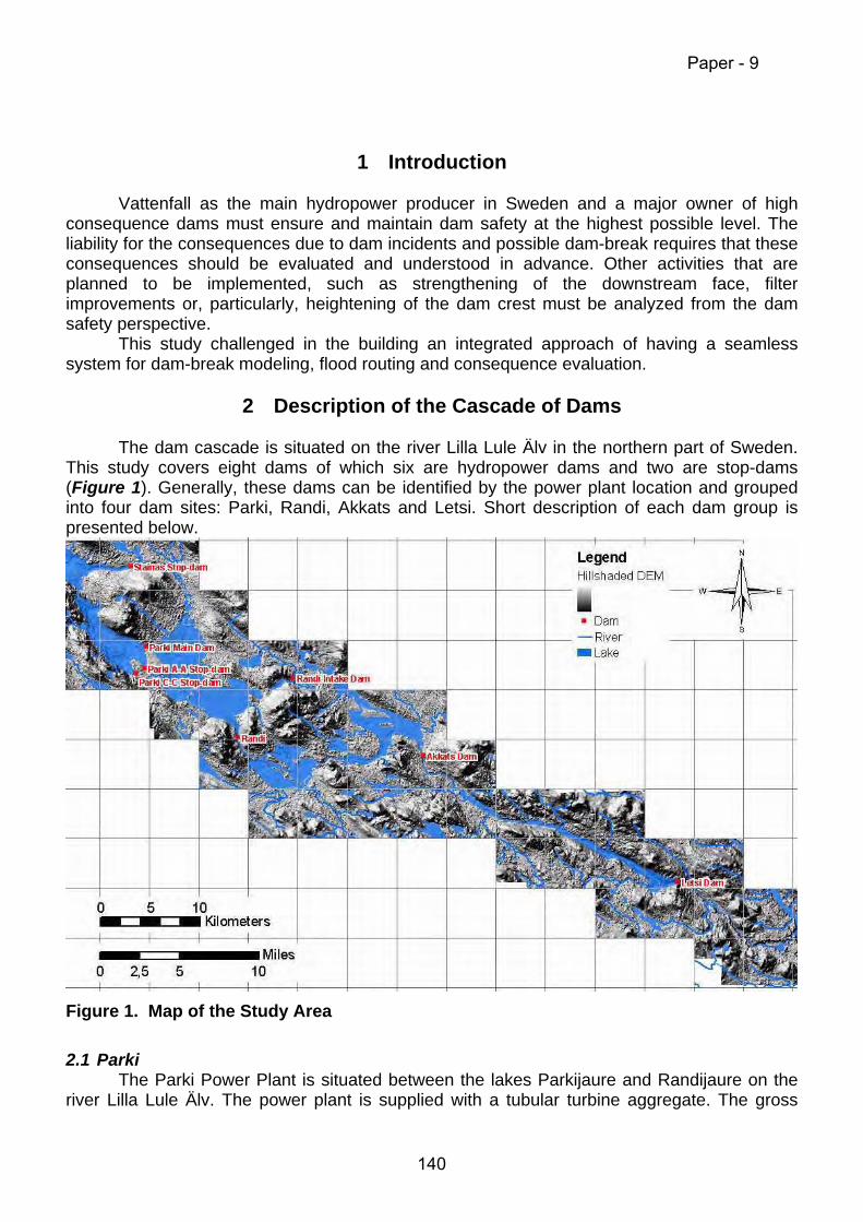
1 Introduction Vattenfall as the main hydropower producer in Sweden and a major owner of high

consequence dams must ensure and maintain dam safety at the highest possible level. The liability for the consequences due to dam incidents and possible dam-break requires that these consequences should be evaluated and understood in advance. Other activities that are planned to be implemented, such as strengthening of the downstream face, filter improvements or, particularly, heightening of the dam crest must be analyzed from the dam safety perspective.

This study challenged in the building an integrated approach of having a seamless system for dam-break modeling, flood routing and consequence evaluation.

2 Description of the Cascade of Dams The dam cascade is situated on the river Lilla Lule Älv in the northern part of Sweden.

This study covers eight dams of which six are hydropower dams and two are stop-dams (Figure 1). Generally, these dams can be identified by the power plant location and grouped into four dam sites: Parki, Randi, Akkats and Letsi. Short description of each dam group is presented below.

Figure 1. Map of the Study Area 2.1 Parki

The Parki Power Plant is situated between the lakes Parkijaure and Randijaure on the river Lilla Lule Älv. The power plant is supplied with a tubular turbine aggregate. The gross

Paper - 9

140

head is 14 m, with a maximum capacity of about 20 MW. The rock fill dam, which is common to the power plant and the regulation of the Lake Skalka, provides a storage capacity of 460 million m3. The power plants construction started during the autumn of 1967 and the plant was taken into service in 1970.

The Parki Power Plant has a main dam with the crest length of 1 900 m, one stop-dam at Stainas with the crest length of 700 m, and three stop-dams at Parkijaure reservoir with the total crest length of about 650 m.

2.2 Randi

The Randi Power Plant is situated between the lakes Randijaure and Vaikijaure on the river Lilla Lule Älv. The gross head is 25 m, with a maximum capacity of about 80 MW. The power plants construction started during the summer of 1973 and the plant was taken into service in 1976.

The Randi Power Plant has an intake dam with the crest length of 100 m and a regulation dam with the crest length of 160 m. There is an intake tunnel of the length of 480 m.

2.3 Akkats

The Akkats power plant is situated on the river Lilla Lule Älv about 4 km from the community of Jokkmokk. The plant is utilizing the gross head between the lake Vaikijaure and the storage of the Letsi power plant. The Gross head is 45.5 m, with a nominal turbine discharge of 385 m3/s and the capacity of about 146 MW.

The dam, which is common to the power plant and the regulation of the lake Vaikijaure, will provide a storage capacity of 42 million m3.

The main dam is constructed as an earth and rock-fill dam and is founded partly on bedrock, partly on moraine. The total length of the dam is 1515 m. A small stop-dam, which length is 240 m, is constructed to the right of the main dam.

Construction was started during the autumn of 1969 and the plant was taken into service during the autumn of 1973.

2.4 Letsi

The Letsi power plant was the first power plant in the river Lilla Lule Älv. The plant is situated about 16 km upstream of the confluence with the river Stora Lule Älv. The plant is utilizing the gross head between the lake Valjates and the storage of the Porsi power plant. The gross head is 136 m, with a nominal turbine discharge of 220 m3/s and a capacity of about 268 MW.

The dam is constructed as an earth and rock-fill dam and is founded on bedrock. The length of the dam crest is 520 m.

Construction was started in the end of 1960 and the plant was taken into operation during the spring of 1976.

3 Integrated Methodology

3.1 General

Various initiatives have been taken earlier in integrating GIS and hydraulic applications in Sweden and elsewhere (Ascila, Brandesten 2002). The methodology developed for this project covers procedures for data collection and processing, hydraulic modeling, GIS integration and modeling, consequence analysis and dissemination of the results.

Paper - 9

141

The different components of work have been linked together in what can be denoted as a methodological framework (Figure 2), which describes the logic of the work and the linkages between work packages and models.

All components used in the methodological framework compound an integrated scalable system which was implemented, tested and used on the Microsoft Windows® 2000 platform.

Figure 2. Methodology Framework The methodology constitutes state-of-the-art, integrated and modular approach for

analyzing consequences related to rivers and watercourses. The core of the framework is the GIS shell in which all geographical data is collected,

stored, analyzed and presented. Coupled to the GIS are industry proven hydraulic models, for the purpose of solving issues and problems within the watercourse.

According to the Figure 2, six Work Packages (WP) are defined: WP1 – Data Collection, WP2 – Site Description, WP3 – Data Processing, WP4 – Hydraulic Modeling, WP5 – Consequence Analysis and WP6 – Information Transfer.

The subsequent chapters include brief introductions and explanations of the modules applied within the scheme; also brief descriptions of tools are given.

Paper - 9

142

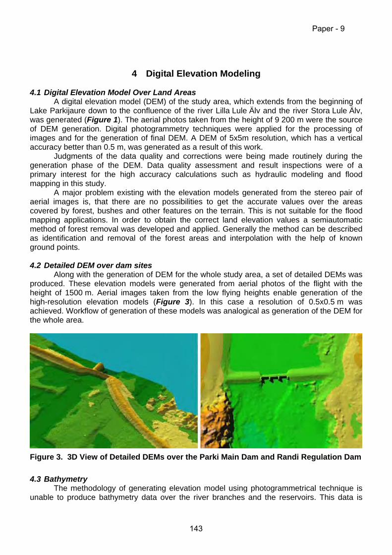
4 Digital Elevation Modeling 4.1 Digital Elevation Model Over Land Areas

A digital elevation model (DEM) of the study area, which extends from the beginning of Lake Parkijaure down to the confluence of the river Lilla Lule Älv and the river Stora Lule Älv, was generated (Figure 1). The aerial photos taken from the height of 9 200 m were the source of DEM generation. Digital photogrammetry techniques were applied for the processing of images and for the generation of final DEM. A DEM of 5x5m resolution, which has a vertical accuracy better than 0.5 m, was generated as a result of this work.

Judgments of the data quality and corrections were being made routinely during the generation phase of the DEM. Data quality assessment and result inspections were of a primary interest for the high accuracy calculations such as hydraulic modeling and flood mapping in this study.

A major problem existing with the elevation models generated from the stereo pair of aerial images is, that there are no possibilities to get the accurate values over the areas covered by forest, bushes and other features on the terrain. This is not suitable for the flood mapping applications. In order to obtain the correct land elevation values a semiautomatic method of forest removal was developed and applied. Generally the method can be described as identification and removal of the forest areas and interpolation with the help of known ground points.

4.2 Detailed DEM over dam sites

Along with the generation of DEM for the whole study area, a set of detailed DEMs was produced. These elevation models were generated from aerial photos of the flight with the height of 1500 m. Aerial images taken from the low flying heights enable generation of the high-resolution elevation models (Figure 3). In this case a resolution of 0.5x0.5 m was achieved. Workflow of generation of these models was analogical as generation of the DEM for the whole area.

Figure 3. 3D View of Detailed DEMs over the Parki Main Dam and Randi Regulation Dam

4.3 Bathymetry

The methodology of generating elevation model using photogrammetrical technique is unable to produce bathymetry data over the river branches and the reservoirs. This data is

Paper - 9

143

very important in order to be able to develop the accurate hydraulic model for simulation of dam-breaks. In this project the bathymetry data was obtained by scanning and digitizing bathymetry maps (Figure 4). All maps were georectified to the common coordinate system to make possible integration with the elevation model over the land area.

Figure 4. Scanned and Georectified Bathymetry Map With Satellite Image in the Background (left) and 3D View of the Digital Bathymetry Data (right)

4.4 Control of Dam Crest Levels with the Help of Detailed DEMs

All dams analyzed in this study were built during the period of 1960-1973. Since the commissioning time some deformations may have occurred. In order to check the values known from the technical documentation a control with the help of the detailed elevation models was carried out. The spatial analysis performed with the help of GIS procedures indicates some declinations from the earlier known values of the dam crests (Figure 5). The new updated values were used as the input for the dam-break initiation levels in the hydraulic model.

Paper - 9

144

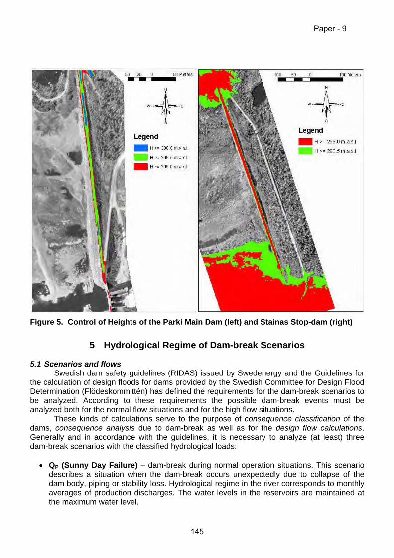
Figure 5. Control of Heights of the Parki Main Dam (left) and Stainas Stop-dam (right)

5 Hydrological Regime of Dam-break Scenarios

5.1 Scenarios and flows

Swedish dam safety guidelines (RIDAS) issued by Swedenergy and the Guidelines for the calculation of design floods for dams provided by the Swedish Committee for Design Flood Determination (Flödeskommittén) has defined the requirements for the dam-break scenarios to be analyzed. According to these requirements the possible dam-break events must be analyzed both for the normal flow situations and for the high flow situations.

These kinds of calculations serve to the purpose of consequence classification of the dams, consequence analysis due to dam-break as well as for the design flow calculations. Generally and in accordance with the guidelines, it is necessary to analyze (at least) three dam-break scenarios with the classified hydrological loads:

• QP (Sunny Day Failure) – dam-break during normal operation situations. This scenario

describes a situation when the dam-break occurs unexpectedly due to collapse of the dam body, piping or stability loss. Hydrological regime in the river corresponds to monthly averages of production discharges. The water levels in the reservoirs are maintained at the maximum water level.

Paper - 9

145

• Q100 (Risk Class 2) – dam-break in combination with the Risk Class 2 flood means that

the dam-break occurs during a flood of 100-year return period. Causes for dam-break can be the same as above, and the initiation of the dam-break may start at the peak of the reservoir lever or at the peak of the flood. Causes for the dam-break can also be a combination of the flood together with failure of operation of the discharge facilities. The flows in the river must correspond to the floods of 100-year probability, which are calculated according to the methodology of calculating Risk Class 2 floods. According to the requirements for Consequence Class 1 (High Consequence Dam) and Consequence Class 2 (Low Consequence Dam) dam facilities, this flow should be possible to discharge at the max water level of the reservoir or, in some cases, slightly more than max water level. Initial water levels in the reservoirs are set up to max water level marker. The initial water levels in the rivers are calculated to be corresponding Risk Class 2 level.

• Q10 000 (Risk Class 1) – dam-break in combination with the Risk Class 1 Flood means

that the dam-break occurs in connection to the extreme flood situation which corresponds to the flow of 10 000 years probability. The causes for dam-break can be the same as both previous scenarios, while the flood will be much higher than Risk Class 2 flood. That means that it can exceed the maximum water level in the reservoir and freeboard leading to overtopping of the dam crest. In those cases when overtopping is not occurring the causes for dam-break are the same as in previous scenarios – peak of the flood or water level in the reservoir. The flows in the river system are based on the flows calculated according to the methodology for calculating of Risk Class 1 floods. The initial water levels in the rivers are calculated to be corresponding Risk Class 1 level.

5.2 Primary and secondary dam breaks or cascading dam-breaks

Most of the Swedish rivers are regulated with many cascading dam facilities. In some cases, the dam-break upstream causes the secondary dam-breaks all the way downstream.

The primary dam-breaks were analyzed in this study for the Parki and Randi dam sites. The secondary dam-breaks may follow as a consequence of a primary dam-break upstream.

The primary dam-break by its nature can be defined as overtopping, piping or stability loss. The secondary dam-break is defined only as overtopping in this study.

5.3 Dam-break initiation and breaching

In the beginning of dam-break calculations it is necessary to describe the situation at which the dam-break initiates. For the overtopping situation, this can be accomplished by defining the reservoir level (usually this corresponds to the lowest dam crest value, but in some cases even the level of the impervious dam core is used). For the piping situation either reservoir water level or the time moment can be used.

It was possible to describe the breaching process by using the parametric approach i.e. a successful breach opening by time or by using the erosion based method.

The erosion-based method was chosen in order to take into account the material properties of the dam. The method is based on the Engelund-Hansen formulation and is built in within the model. To define the maximum size of the breach opening limiting sections were identified. The erosion based approach was used both for simulation of breaching caused by overtopping and piping.

Paper - 9

146

5.4 Regulation strategies under the dam-break situation

Different regulation strategies can lead to significant differences regarding the consequences due to dam-break. Realistic and conservative assumptions were applied when defining the regulation strategies under the different dam-break situations. Special emphasis was laid on existing instructions for regulation strategies, which are used in the real world situations when the dam-break incidents happen. These are the following:

Main principles of regulation strategies: 1. Appropriate initial conditions in the river and in the reservoirs. This links to the

descriptions of different hydrological load scenarios and flows. 2. It is assumed that the electricity production stops under the dam-break situation. 3. With the increasing inflows the spillway gates opens gradually until the full spillage is

reached. 4. It is assumed that the gates cannot be operated when the dam-break occurs on the

same facility. The level of the gates remains at the same position as before the dam-break initiation.

5. It is assumed that opening of gates of the downstream spillway is possible when the primary dam-break occurs. This allows the spilling of water from the downstream water storages and thus freeing some storage for the dam-break flood.

6 Linking of Hydraulic Model and GIS Hydraulic modeling and GIS technology become more powerful when they are coupled

into an integrated system. This combination enables bi-directional data exchange; modeling is performed in the common geographic reference system, and once the system is developed, data update procedures become simple and effective.

One of the most valuable and efficient procedures using this approach is the possibility of automatic extraction of the hydraulic parameters from digital elevation model. Among various parameters available, the most important for hydraulic modeling are river geomorphologic characteristics, representing the geometry of riverbed and floodplain.

In this study all data was prepared and stored in the GIS shell. This enables the efficiency in maintaining and sharing data for the various purposes within this project. As indicated in the methodology, the integration of the hydraulic model into GIS was possible by using pre- and post-processing routines. They enabled bi-directional integrated communications between GIS and hydraulic model.

The major advantages of this integration were the possibilities to automatically prepare the cross-section database and to import it into hydraulic model. Data generated by the hydraulic model was transferred to the GIS in order to perform further analysis.

7 Hydraulic Modeling

7.1 Hydraulic Model As indicated in the Methodological Framework (Figure 2), different hydraulic models

can be applied for the 1-D flood routing, such as HEC-RAS, DAMBRK or MIKE 11, for the 1-D flood routing. It was decided to use MIKE 11 hydrodynamic model for this study. MIKE 11 is a 1-D model used for the simulation of hydrodynamic flow and sediment transport. More information about the model can be found in the references.

Paper - 9

147

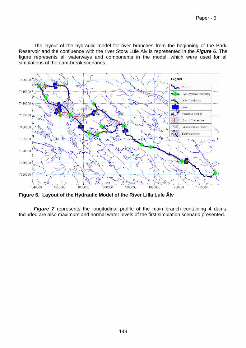
The layout of the hydraulic model for river branches from the beginning of the Parki Reservoir and the confluence with the river Stora Lule Älv is represented in the Figure 6. The figure represents all waterways and components in the model, which were used for all simulations of the dam-break scenarios.

Figure 6. Layout of the Hydraulic Model of the River Lilla Lule Älv

Figure 7 represents the longitudinal profile of the main branch containing 4 dams.

Included are also maximum and normal water levels of the first simulation scenario presented.

Paper - 9

148

Figure 7. Plot of Longitudinal Profile of the Dam Cascade

7.2 Model calibration

Control calculations have been performed in order to calibrate the model to obtain the accurate water levels, which were known from earlier hydrological simulations. Model was calibrated by using the flow resistance values, which were associated to the land cover information available as a GIS layer.

8 Modeling Results and Discussion

8.1 General

By utilizing the methods and techniques described in this paper, 16 dam-break scenarios were analyzed in this study. The content of some of the scenarios was obvious in the beginning, while the other scenarios have evolved after summarizing the results of previous ones. That means, that besides the analysis of current situation in the river system, a set of “what-if?” cases were analyzed. Due to limited extent of this paper, only the most significant scenarios are presented in this chapter. For the same reason only fragments of the inundation maps are presented in this chapter and these cover only the “hot spots” in the area.

8.2 Present Conditions with the Risk Class 1 Flood

This scenario covers the analysis of the dams with the present properties and Risk Class 1 flood used as a hydrological load. By routing this flood trough the river system it was concluded that two dams in the system couldn’t pass the flood and were overtopped.

Paper - 9

149

These were the Stainas Stop-Dam and the Randi Intake Dam. The breaching of these dams resulted, however, in no secondary dam-breaks in the dam cascade.

Further analysis of third party consequences indicated that these two dams should be categorized as low consequence dams that require a design flood capacity of the 100-year probability.

Figure 8. Inundation due to Primary Dam-break in Stainas Stop-dam and Secondary

Dam-break in Randi Intake Dam under the Risk Class 2 Hydrological Conditions

8.3 Heightening of the Stainas Stop-dam and Randi Dams

This scenario evolves as a natural step after obtaining the results from the scenario described in the previous chapter, i.e. it has been necessary to model what would be the consequences if the dams that breached were heightened to the level capable to pass through the Risk Class 1 flood. After the describing of these measures in the model it was possible to simulate how the heightening of the dams would change the inundation and the consequences. The difference of the consequences is presented in the next chapter while the visual representation is provided in the Figure 9.

Paper - 9

150

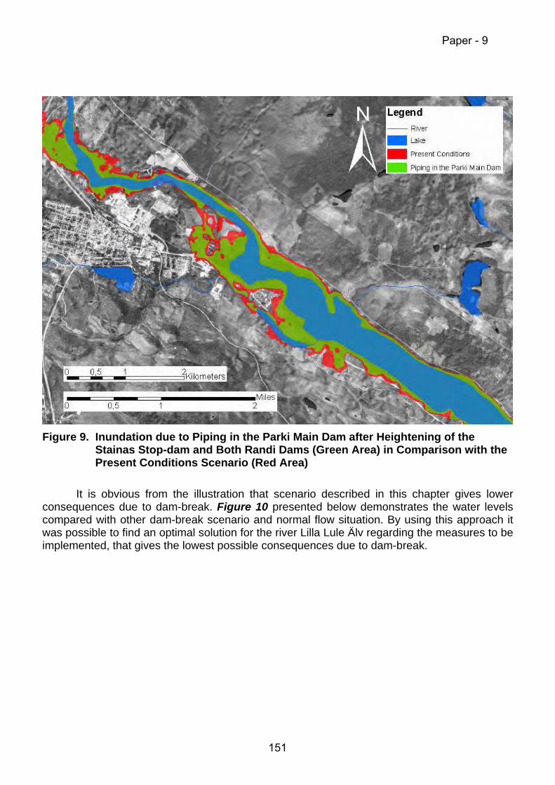
Figure 9. Inundation due to Piping in the Parki Main Dam after Heightening of the

Stainas Stop-dam and Both Randi Dams (Green Area) in Comparison with the Present Conditions Scenario (Red Area)

It is obvious from the illustration that scenario described in this chapter gives lower

consequences due to dam-break. Figure 10 presented below demonstrates the water levels compared with other dam-break scenario and normal flow situation. By using this approach it was possible to find an optimal solution for the river Lilla Lule Älv regarding the measures to be implemented, that gives the lowest possible consequences due to dam-break.

Paper - 9

151

13-8-1981 15-8-1981 17-8-1981 19-8-1981 21-8-1981 23-8-1981 25-8-1981217.0

217.5

218.0

218.5

219.0

219.5

220.0

220.5

221.0

221.5

Water Level (m.a.s.l.) Comparison of the Water Levels of Three Dam-break Scenarios

Figure 10. Water Level Comparison

9 Consequence Evaluation

Based on the information gathered from the hydraulic model in the GIS it is possible to determine the aerial extent of various land-types as well as individual objects that will be flooded as a consequence of dam-break. These consequences were analyzed within GIS application and some of the major scenarios are summarized in the Table 1 below: Table 1. Summary of the Consequences of Characteristic Dam-break Scenarios

Inun

datio

n (h

a)

Dw

ellin

g H

ouse

s (U

nits

Affe

cted

)

Aux

iliary

Bui

ldin

gs

(Uni

ts A

ffect

ed)

Tran

sfor

mer

St

atio

ns (U

nits

A

ffect

ed)

Rai

lroad

s (k

m)

Roa

ds (k

m)

Pow

er L

ines

(km

)

Reference Scenarios Without Dam-break Scenario 10. Reference QP 0 0 0 0 0 0 0 Scenario 9. Reference Q100 (Risk Class 2 Flood) 622 15 29 0 0 26 10 Dam-break Scenarios with Risk Class 1 Flood (Q10 000) Scenario 1. Current Conditions 1700 75 103 2 24 202 212Scenario 2. Current conditions and piping in Parki Main Dam 2833 134 169 2 19 528 306

Water Level in Present Conditions Scenario

Normal Water Level

Water Level due to Piping in Parki Main Dam after heightening of the Stainas Stop-dam and Both Randi Dams

Paper - 9

152

Scenario 5. Stainas Stop-dam and both Randi dams are heightened and piping in Parki Main Dam 2667 100 130 3 22 221 254Scenario 7. Stainas Stop-dam and all Parki dams are heightened and piping in Randi Regulation Dam 1750 81 110 3 24 215 160Dam-break Scenario with Risk Class 2 Flood (Q100) Scenario 11. Piping in Randi Intake Dam 553 12 26 0 0 32 8

10 Conclusions This study demonstrates the efficiency of the methods of applying an integrated

approach by combining different technologies in order to understand how the regulated waterways are functioning. By having this understanding and by having the data necessary it is possible to make the decisions which are based on the material of high accuracy. This leads to better solutions when implementing dam safety measures or when dealing with other tasks such as emergency planning.

All dam facilities are described in one model, which enables simulation of the whole river system i.e. the cascading dam-breaks, which leads to better understanding of possible consequences of such event.

Results from the study presented in this paper demonstrated that hydrological upgrading is necessary for the Parki main dam. At present pre-studies on the hydrological upgrading, as well as general dam safety improvements are about to be initiated at both Parki and Randi facilities.

It is planned to maintain the system for the future applications by adding new features and by updating data.

11 References

1. Parki – Technical Data (1968). Swedish State Power Board. 2. Randi kraftstation (1974). Vattenfall (in Swedish). 3. Parki – Technical Data (1971). Swedish State Power Board. 4. Parki – Technical Data (1971). Swedish State Power Board. 5. Consequence Analysis due to Dam-break: A Pilot Study for Messaure (2002). Report.

SwedPower. 6. RIDAS - Swedish Dam Safety Guidelines (2002), Swedenergy AB. 7. Flödeskommittén - Riktlinjer för bestämning av dimensionerande flöden för

dammanläggningar (1990). (In Swedish: Guidelines for the calculation of design floods for dams). Final report from the Swedish Committee for Design Flood Determination. Swedish State Power Board, Swedish Power Association and Swedish Meteorological and Hydrological Institute, Stockholm and Norrköping, Sweden.

8. MIKE 11 – Users Guide (2003). DHI Water & Environment. 9. MIKE 11 – Reference Manual (2003). DHI Water & Environment. 10. Flodvågsberäkning för Luleälven (1997). Vattenfall Hydropower AB. (In Swedish: Hydraulic

calculations for river Lule Älv) 11. Flodvågsberäkning vid klass 2 flöde för 10 dammar i Luleälven (1997). Vattenfall

Hydropower AB. (In Swedish: Hydraulic calculations with the Risk Class 2 flow for 10 dams in the river Lule Älv)

Paper - 9

153

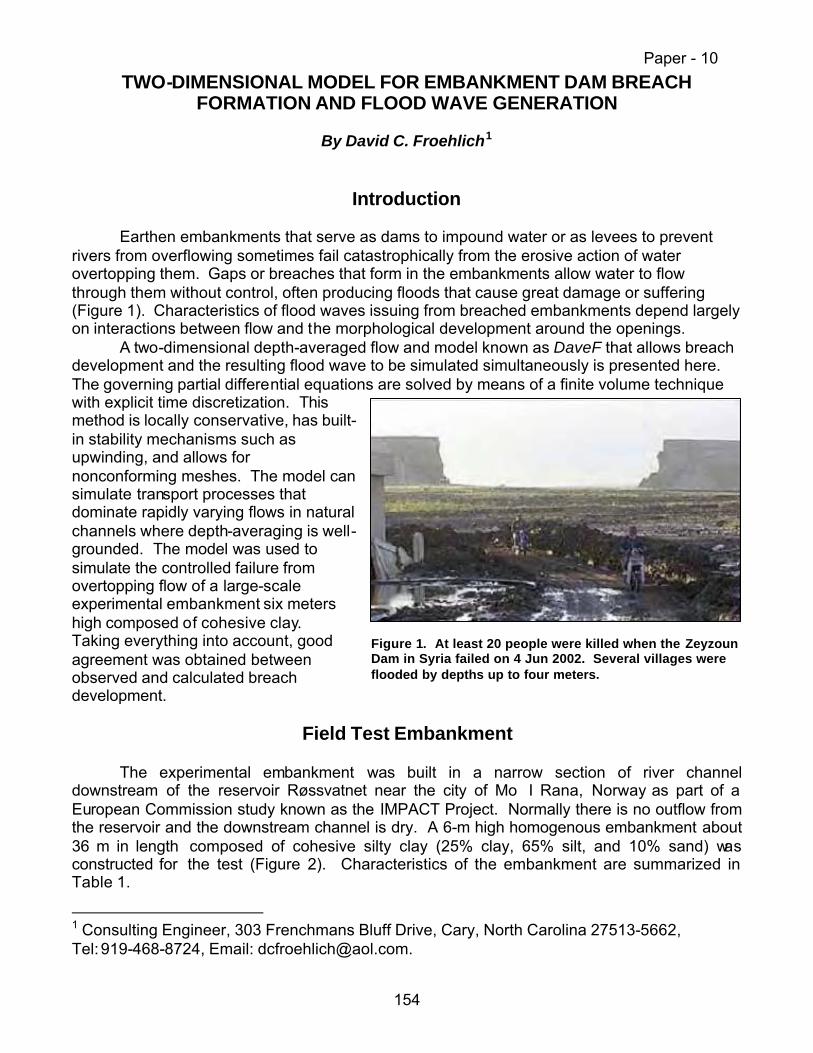
TWO-DIMENSIONAL MODEL FOR EMBANKMENT DAM BREACH FORMATION AND FLOOD WAVE GENERATION

By David C. Froehlich1

Introduction

Earthen embankments that serve as dams to impound water or as levees to prevent rivers from overflowing sometimes fail catastrophically from the erosive action of water overtopping them. Gaps or breaches that form in the embankments allow water to flow through them without control, often producing floods that cause great damage or suffering (Figure 1). Characteristics of flood waves issuing from breached embankments depend largely on interactions between flow and the morphological development around the openings.

A two-dimensional depth-averaged flow and model known as DaveF that allows breach development and the resulting flood wave to be simulated simultaneously is presented here. The governing partial differential equations are solved by means of a finite volume technique with explicit time discretization. This method is locally conservative, has built-in stability mechanisms such as upwinding, and allows for nonconforming meshes. The model can simulate transport processes that dominate rapidly varying flows in natural channels where depth-averaging is well-grounded. The model was used to simulate the controlled failure from overtopping flow of a large-scale experimental embankment six meters high composed of cohesive clay. Taking everything into account, good agreement was obtained between observed and calculated breach development.

Field Test Embankment

The experimental embankment was built in a narrow section of river channel

downstream of the reservoir Røssvatnet near the city of Mo I Rana, Norway as part of a European Commission study known as the IMPACT Project. Normally there is no outflow from the reservoir and the downstream channel is dry. A 6-m high homogenous embankment about 36 m in length composed of cohesive silty clay (25% clay, 65% silt, and 10% sand) was constructed for the test (Figure 2). Characteristics of the embankment are summarized in Table 1.

1 Consulting Engineer, 303 Frenchmans Bluff Drive, Cary, North Carolina 27513-5662, Tel: 919-468-8724, Email: dcfroehlich@aol.com.

Figure 1. At least 20 people were killed when the Zeyzoun Dam in Syria failed on 4 Jun 2002. Several villages were flooded by depths up to four meters.

Paper - 10

154

To initiate breaching, a notch 0.5 m deep and about 2 m wide was cut through the center of embankment crests. Impoundments behind the embankments were filled to crest level, and upstream water-surface elevations were held nearly constant during the initial overtopping. Parameters for the test embankment are summarized in Table 1.

.

Table 1. Experimental Embankment Characteristics

Embankment parameter Value Height 6.0 m Crest elevation 670.81 m Crest width 2.0 m Crest length 36.0 m Embankment slope: Upstream 2:1 Downstream 2:1 Median grain size, D50 0.010 mm Porosity 0.200 Dry unit weight, ?d 17,000 N Friction angle, f 10o Cohesion 25,000 N/m2

Plasticity index 15 Manning coefficient, n 0.030

Figure 2. Experimental embankment at test site near Mo I Rana, Norway just before start of overtopping

Paper - 10

155

Governing Equations

The numerical model is based on conservation forms of the depth-averaged fluid, and

momentum transport relations, which comprise a coupled system of nonlinear, hyperbolic, partial differential equations as follows:

[ ( ), ( )] 0t

∂+ ∇ ⋅ + =

∂U F U G U Q (1)

where

1 22

21 1 21

221 2 22

01 12

1 12

bbx

bby

q qh

zq q qq gh gh

h h xq q q q zgh ghh h y

τρ

τρ

∂ = = + = = +

∂ ∂+ + ∂

U F G Q (2)

t = time, h = water depth, q1 and q2 = unit flow rates in the horizontal x and y Cartesian coordinate directions respectively, 2 2

1 2q q q= + = total unit flow rate, g = gravitational acceleration, zb = bed elevation, ρ = water mass density, and t bx and t by = bed shear stresses in the x and y directions respectively. Bed shear stresses are given by

2 2 2 21 1 2 2 1 2

2 2andbx f b by f bq q q q q q

c m c mh h

τ ρ τ ρ+ +

= = (3)

where

2

2 1 / 3fgnc

hψ= (4)

Is a dimensionless bed friction factor, n = Manning’s roughness coefficient, ? = units factor (1.0 for SI, 1.486 for U.S. Customary), and

22

1 b bb

z zm

x y∂ ∂

= + + ∂ ∂ (5)

is a coefficient that accounts for a sloping bed. defined, although some guidance is available

Paper - 10

156

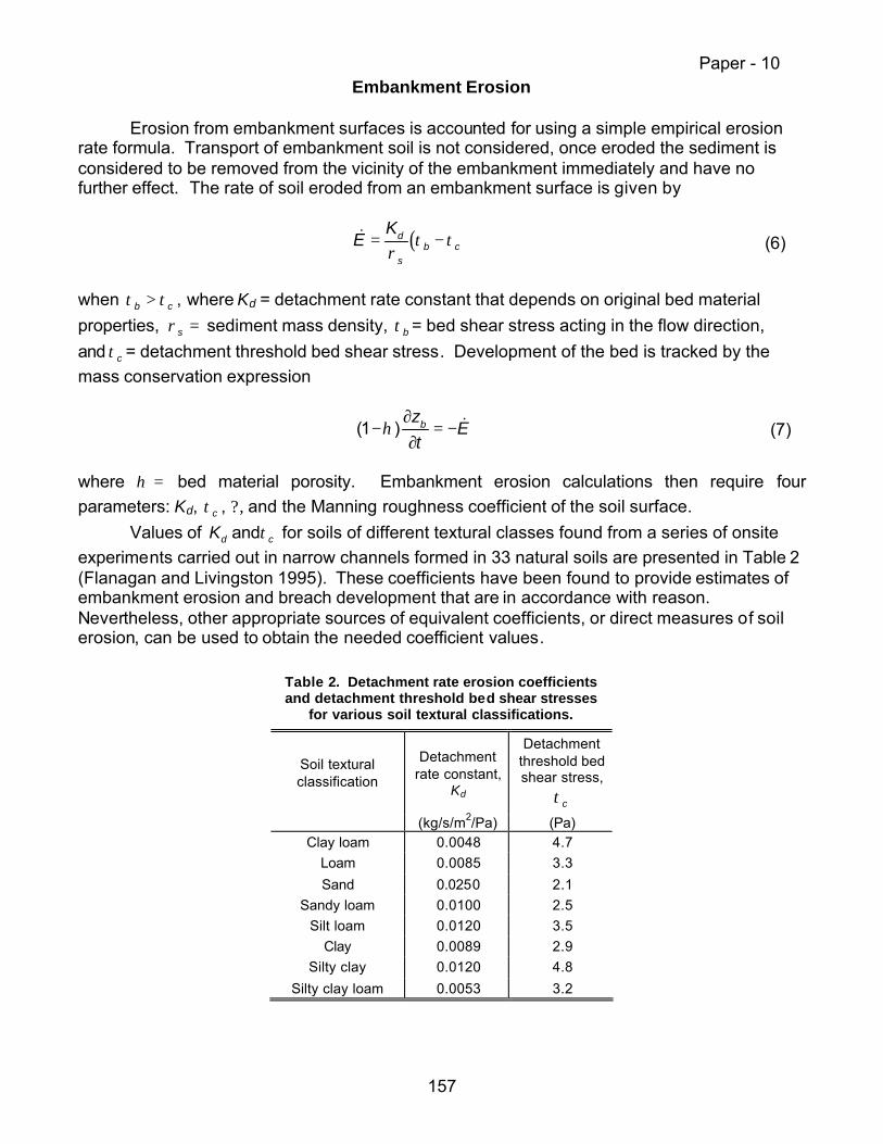
Embankment Erosion

Erosion from embankment surfaces is accounted for using a simple empirical erosion rate formula. Transport of embankment soil is not considered, once eroded the sediment is considered to be removed from the vicinity of the embankment immediately and have no further effect. The rate of soil eroded from an embankment surface is given by

( )db c

s

KE τ τ

ρ= −& (6)

when b cτ τ> , where Kd = detachment rate constant that depends on original bed material properties, sρ = sediment mass density, bτ = bed shear stress acting in the flow direction, and cτ = detachment threshold bed shear stress. Development of the bed is tracked by the mass conservation expression

(1 ) bzE

tη

∂− = −

∂& (7)

where η = bed material porosity. Embankment erosion calculations then require four parameters: Kd, cτ , ?, and the Manning roughness coefficient of the soil surface.

Values of andd cK τ for soils of different textural classes found from a series of onsite experiments carried out in narrow channels formed in 33 natural soils are presented in Table 2 (Flanagan and Livingston 1995). These coefficients have been found to provide estimates of embankment erosion and breach development that are in accordance with reason. Nevertheless, other appropriate sources of equivalent coefficients, or direct measures of soil erosion, can be used to obtain the needed coefficient values.

Table 2. Detachment rate erosion coefficients and detachment threshold bed shear stresses

for various soil textural classifications.

Soil textural classification

Detachment rate constant,

Kd

Detachment threshold bed shear stress,

cτ

(kg/s/m2/Pa) (Pa) Clay loam 0.0048 4.7

Loam 0.0085 3.3 Sand 0.0250 2.1

Sandy loam 0.0100 2.5 Silt loam 0.0120 3.5

Clay 0.0089 2.9 Silty clay 0.0120 4.8

Silty clay loam 0.0053 3.2

Paper - 10

157

Model Formulation

The depth-averaged surface-water flow and sediment transport equations are solved numerically using a two-dimensional, cell-centered, Godunov-type, finite volume scheme. Godunov-type methods for solving first-order hyperbolic systems of equations are based on solutions of initial value problems, known as Riemann problems, involving discontinuous neighboring states. These methods are found to be accurate and robust when used to solve partial differential equations describing fluid motion, being able to capture locations of shocks and contact surfaces.

Values of the conserved variables are calculated for each of the volumes or cells. Cells can be any convex polygon, but are limited in DaveF to triangles and quadrilaterals. Bed slope source terms are taken into account by combining them with edge fluxes in a manner that leads to proper balance of forces.

Discretization of integral forms of the conservation equations (1) by the finite volume method assures that the basic quantities, mass and momentum, will be conserved across discontinuities (Hirsch 1988). Applying the divergence theorem to (1) and integrating over an arbitrary cell Ei gives the basic finite volume equation

[ ( ) ( )] 0i i iE E E

dA dS dAt ∂

∂+ ⋅ + =

∂ ∫ ∫ ∫U F U , G U n QÑ (8)

where 1 2[ , ] [cos ,sin ]n n θ θ≡ ≡ =n outward unit normal vector to the boundary Si, ? = angle between the positive x direction and the vector n, and dA and dS are the area and boundary elements of the cell, respectively. Making use of the rotational invariance property of (1) (Toro 2001, p. 65), the normal flux component through a surface is given by

1[ ( ), ( )] ( )−⋅ =n F U G U T F TU (9) where T = T(?) = rotation matrix given as

1 0 00 cos sin0 sin cos

θ θθ θ

= −

T (10)

Using the normal flux expression given by (9), the integral relation (8) becomes

1 ( ) 0i i iE E E

dA dS dAt

−

∂

∂+ + =

∂ ∫ ∫ ∫U T F TU QÑ (11)

Within each cell U is considered to be constant, and the flux across any edge is based on the states in the two adjacent cells. Letting ≡ =U TU% variables transformed to the edge-normal/tangential directions, (11) becomes

Paper - 10

158

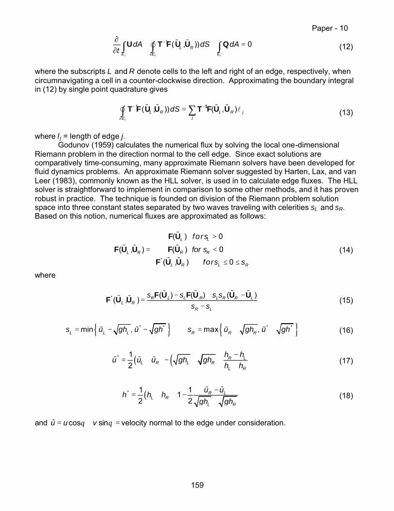
1 ( , )) 0i i i

L RE E E

dA dS dAt

−

∂

∂+ + =

∂ ∫ ∫ ∫U T F U U Q% %Ñ (12)

where the subscripts L and R denote cells to the left and right of an edge, respectively, when circumnavigating a cell in a counter-clockwise direction. Approximating the boundary integral in (12) by single point quadrature gives

1 ( , )) ( , )i

L R L R jjE

dS− −

∂

= ∑∫ 1T F U U T F U U% % % % lÑ (13)

where l j = length of edge j.

Godunov (1959) calculates the numerical flux by solving the local one-dimensional Riemann problem in the direction normal to the cell edge. Since exact solutions are comparatively time-consuming, many approximate Riemann solvers have been developed for fluid dynamics problems. An approximate Riemann solver suggested by Harten, Lax, and van Leer (1983), commonly known as the HLL solver, is used in to calculate edge fluxes. The HLL solver is straightforward to implement in comparison to some other methods, and it has proven robust in practice. The technique is founded on division of the Riemann problem solution space into three constant states separated by two waves traveling with celerities sL and sR. Based on this notion, numerical fluxes are approximated as follows:

*

( ) 0

( , ) ( ) 0( , ) 0

L L

L R R R

L R L R

fo rs

for sfors s

>

= < ≤ ≤

F UF U U F U

F U U

%% % %

% % (14)

where

* ( ) ( ) ( )( , ) R L L R L R R LL R

R L

s s s ss s

− + −=

−F U F U U UF U U

% % % %% % (15)

{ } { }* * * *min , max ,L L L R R Rs u gh u gh s u gh u gh= − − = + +% % % % (16)

( ) ( )* 12

R LL R L R

L R

h hu u u gh gh

h h −

= + − + + % % % (17)

( )* 1 112 2

R LL R

L R

u uh h hgh gh

−= + − +

% % (18)

and cos sinu u vθ θ= + =% velocity normal to the edge under consideration.

Paper - 10

159

Bed Slope Terms

Centered approximation of bed slope source terms in (12) unfortunately leads to unbalanced forces for non-horizontal beds, which prevents retrieval of trivial solutions having horizontal water surfaces and motionless states when only no-flux boundary conditions are applied around the computational mesh. Bermúdez and Vázquez-Cendón (1994), Bermúdez et al. (1996) and Leveque (1998) address this predicament for other Godunov-type finite volume schemes. To provide a proper balance of pressure and gravitational forces using the HLL solver, bed slope terms are merged with edge flux vectors as follows:

where ( )′F U% = modified normal flux vector. Source terms are modified accordingly as

The finite volume problem statement then becomes

( , ) 0i i

L R jjE E

dA dAt

−∂ ′ ′+ + =∂ ∑∫ ∫1U T F U U Q% % l (21)

with ( )F U% replaced by ( )′F U% in (14) and (15).

Solution of the Discrete System

The local one-dimensional problem given by (21) is solved using Strang splitting (1968) whereby the pure advection problem given by the homogeneous part, that is,

( , ) 0i

L R jjE

dAt

−∂ ′+ =∂ ∑∫ 1U T F U U% % l (22)

is solved first by evaluating the area integral and applying forward Euler time integration to obtain

01

( ) ( ) ( )( )2

0

L R bR bLg h h z z

′ = + + −

F U F U% % (19)

01

1

bx

by

τρ

τρ

′ =

Q (20)

Paper - 10

160

where advi =U the advection-only solution. This is followed by solution of the ordinary

differential equation

that accounts for source terms due to bed friction and sediment erosion/deposition. Solving (24) with forward Euler time integration gives

which is considered to be the standard splitting scheme (Toro 2001, p. 233).

The Field Test Model

A computational mesh consisting of a mixture of triangular and quadrilateral cells covering a 300 m length of river channel was used to simulate overtopping flow and breach development (Figure 3). Bed elevations defined by the mesh are shown in Figure 4. Erosive soil was modeled only in embankment areas, although eroded embankment soils deposited

downstream could be re-entrained and transported further downstream.

Initial conditions consisted of a level water-surface equal to the embankment crest elevations and motionless states in the upstream channel. Constant head boundary conditions maintaining the initial water-surface elevations were applied at the upstream end of the channel in each case, and free-outfall conditions (that is, critical depth) was set at the downstream end.

( , )adv ni i L R j

ji

tA

− ∆′= −

∑ 1U U T F U U% % l (23)

( ) 0advii

ddt

′+ =U Q U (24)

1 ( , ) ( ) 0n n advi i L R j i

ji

tt

A+ − ∆

′ ′= − − ∆ = ∑ 1U U T F U U Q U% % l (25)

Figure 3. Finite volume mesh consisting of triangles and quadrilaterals covering a 300 m section of river channel containing the test embankment.

Figure 4. Color contours showing bed elevations represented in the field test finite volume mesh. Water flows from the bottom to top of the

Paper - 10

161

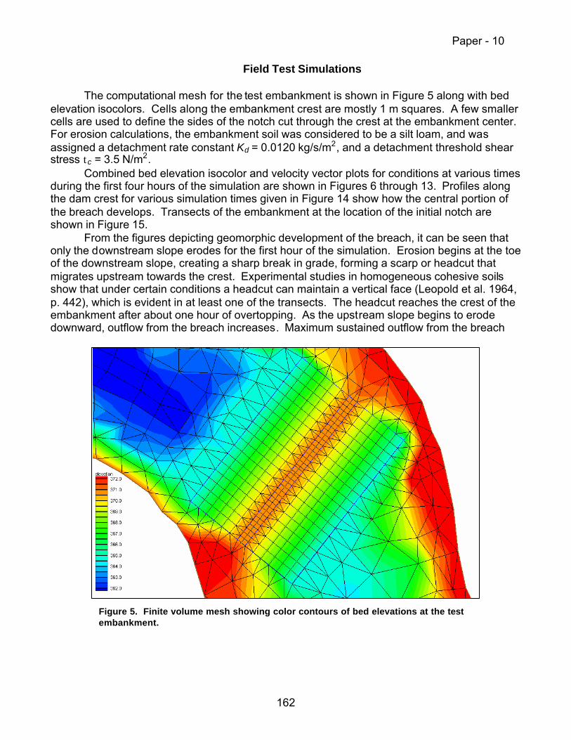
Field Test Simulations

The computational mesh for the test embankment is shown in Figure 5 along with bed

elevation isocolors. Cells along the embankment crest are mostly 1 m squares. A few smaller cells are used to define the sides of the notch cut through the crest at the embankment center. For erosion calculations, the embankment soil was considered to be a silt loam, and was assigned a detachment rate constant Kd = 0.0120 kg/s/m2, and a detachment threshold shear stress tc = 3.5 N/m2.

Combined bed elevation isocolor and velocity vector plots for conditions at various times during the first four hours of the simulation are shown in Figures 6 through 13. Profiles along the dam crest for various simulation times given in Figure 14 show how the central portion of the breach develops. Transects of the embankment at the location of the initial notch are shown in Figure 15.

From the figures depicting geomorphic development of the breach, it can be seen that only the downstream slope erodes for the first hour of the simulation. Erosion begins at the toe of the downstream slope, creating a sharp break in grade, forming a scarp or headcut that migrates upstream towards the crest. Experimental studies in homogeneous cohesive soils show that under certain conditions a headcut can maintain a vertical face (Leopold et al. 1964, p. 442), which is evident in at least one of the transects. The headcut reaches the crest of the embankment after about one hour of overtopping. As the upstream slope begins to erode downward, outflow from the breach increases. Maximum sustained outflow from the breach

Figure 5. Finite volume mesh showing color contours of bed elevations at the test embankment.

Paper - 10

162

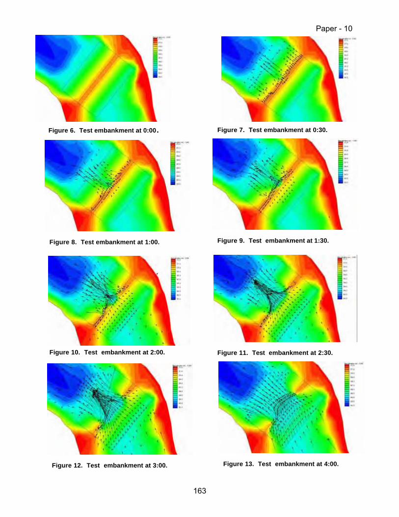
Figure 6. Test embankment at 0:00.

Figure 7. Test embankment at 0:30.

Figure 8. Test embankment at 1:00. Figure 9. Test embankment at 1:30.

Figure 10. Test embankment at 2:00. Figure 11. Test embankment at 2:30.

Figure 12. Test embankment at 3:00. Figure 13. Test embankment at 4:00.

Paper - 10

163

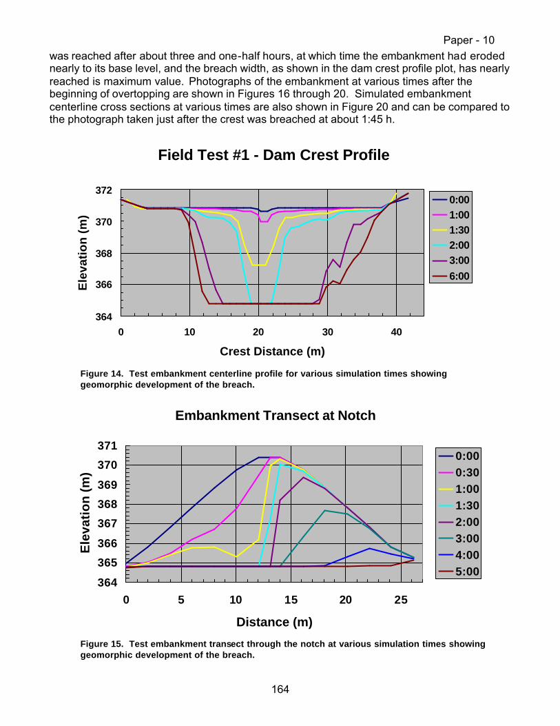
was reached after about three and one-half hours, at which time the embankment had eroded nearly to its base level, and the breach width, as shown in the dam crest profile plot, has nearly reached is maximum value. Photographs of the embankment at various times after the beginning of overtopping are shown in Figures 16 through 20. Simulated embankment centerline cross sections at various times are also shown in Figure 20 and can be compared to the photograph taken just after the crest was breached at about 1:45 h.

Field Test #1 - Dam Crest Profile

364

366

368

370

372

0 10 20 30 40

Crest Distance (m)

Elev

atio

n (m

)

0:001:001:302:003:006:00

Figure 14. Test embankment centerline profile for various simulation times showing geomorphic development of the breach.

Embankment Transect at Notch

364365366367368369370371

0 5 10 15 20 25

Distance (m)

Elev

atio

n (m

)

0:000:301:001:302:003:004:005:00

Figure 15. Test embankment transect through the notch at various simulation times showing geomorphic development of the breach.

Paper - 10

164

Figure 16. Start of over overtopping flow.

Figure 17. Beginning of erosion at the toe of the embankment as headcuts are formed.

Paper - 10

165

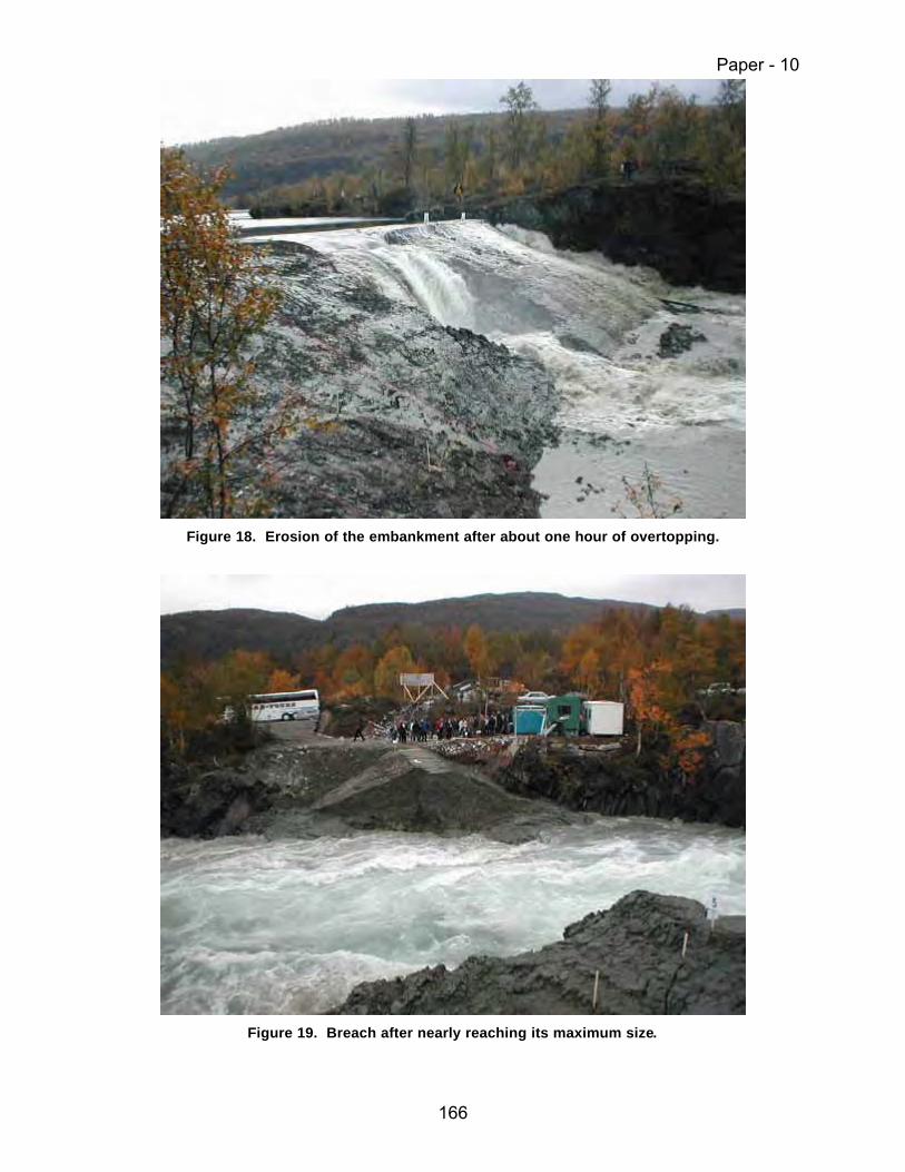
Figure 18. Erosion of the embankment after about one hour of overtopping.

Figure 19. Breach after nearly reaching its maximum size.

Paper - 10

166

Figure 20. Embankment cross sections at various times and photograph of embankment as the embankment crest is breached, about time 1:45.

Summary and Conclusions

Erosion of a large-scale experimental earthen embankment from erosion by overtopping was simulated using a two-dimensional depth-averaged flow model that allows breach development and the resulting flood wave to be simulated simultaneously. The governing partial differential equations were solved by means of a Godunov-type finite volume technique using an approximate Riemann solver. The model can simulate all transport processes that dominate rapidly varying flows in natural channels where depth-averaging is well-grounded.

The model also shows that erosion began at the toe of the downstream slope, creating distinct scarps or headcuts that migrated upstream towards the embankment crest, as observed during the test. The numerical simulations also predict the test embankment to form in the general shape of a trapezoid, first eroding downward to an erosion resistant base level, and then expanding laterally, also as observed. Taking everything into account, good agreement was obtained between the observed breach development and the calculated embankment erosion and flood wave generation.

Paper - 10

167

References

Bermúdez, A., and Vázquez, M. E. (1994). “Upwind methods for hyperbolic conservation laws with source terms.” Computers and Fluids, 23, 1049-1071.

Bermúdez, A., Dervieux, A., Désidéri, J. A., and Vázquez, M. E. (1995). “Upwind schemes for

the two-dimensional shallow water equations with variable depth using unstructured meshes.” Computer Methods in Applied mechanics and Engineering, 155, 49-72.

Flanagan, D. C., and Livingston, S. J. (1995). “WEPP user summary.” NSERL Report No. 11,

National Soil Erosion Research Laboratory, U.S. Department of Agriculture, Agricultural Research Service, West Lafayette, Indiana.

Froehlich, D. C. (1995). “Embankment dam breach parameters revisited.” Proceedings of the

First International Conference on Water Resources Engineering, San Antonio, Texas, August 14-18, 1995, American Society of Civil Engineers, New York, NY, 887-891.

Godunov, S. K. (1959). “A difference scheme for numerical computation of discontinuous

solutions of hydrodynamics equations.” Matemsticheskly Sboraik, 47 (translated by U.S. Joint Publications research Service).

Harten, A., Lax, P. D., and van Leer, B. (1983). “On upstream differencing and Godunov-type

schemes for hyperbolic conservation laws.” SIAM Review, 25(1), 35-61. Hirsch, C. (1988) Numerical computation of internal and external flows, volume 1,

fundamentals of numerical discretization. John Wiley and Sons, new York, New York. Leopold, L. B., Wolman, M. G., and Miller, J. P. (1964). Fluvial processes in geomorphology.

W. H. Freeman and Company, San Francisco, California. LeVeque, R. J. (1998). “Balancing source terms and flux gradients in high-resolution Godunov

methods: the quasi-steady wave-propagation algorithm.” Journal of Computational Physics, 146, 346-365.

Pugh, C. A. (1985). “Hydraulic model studies of fuseplug embankments.” Report No. REC-

ERC-85-7, U.S. Department of the Interior, Bureau of Reclamation, Denver, Colorado. Roe, P. L. (1981). “Approximate Riemann solvers, parameter vectors, and difference

schemes.” Journal of Computational Physics, 43, 357-372. Strang, G. (1968). “On the construction and comparison of finite difference schemes.” SIAM

Journal on Numerical Analysis, 5(3), 506-517. Toro, E. F. (1997). Riemann solvers and numerical methods for fluid dynamics: a practical

introduction. Springer-Verlag, Berlin. Toro, E. F. (2001). Shock-capturing methods for free-surface shallow flows . John Wiley and

Sons, Chichester, United Kingdom.

Paper - 10

168