the modelling of oil agglomeration of coal fines

Journal of Computational and Applied Mathematics 28 (1989) 359-366 North-Holland

359

The modelling of oil agglomeration of coal fines

J. SPOELSTRA Department of Mathematics and Applied Mathematics, Potchefstroom University for CHE, Private Bag X6001, 2520 Potchefstroom, S. Africa

Received 20 May 1988 Revised 24 January 1989

Abstract: Coal-oil agglomeration is an emerging process in the treatment of coal fines. In this paper a mathematical model for the agglomeration growth is constructed. In the model the rate at which individual coal particles get coated with oil, and the rate at which they consequently agglomerate with other coated particles are considered as two separate steps in the agglomeration process. Parameters characterising the process are introduced and the prediction of the model for the resultant growth in agglomerate size is discussed.

Keywords: Mathematical modelling, agglomeration.

1. Introduction

In the coal-oil agglomeration process for refining coal, oil is added to an agitated coal slurry. The hydrophobic coal particles are wetted with the oil, but not the hydrophilic clay particles and other residues. The coal particles then agglomerate into particles large enough to be separated from the residues by means of a sieve.

Quite a number of laboratory and pilot plant investigations into the process have been carried out, investigating different factors affecting the yield [1,4]. This method is arguably the only promising method that can be successfully used for the treatment when most of the fines are smaller than 200 mesh, for lower-rank coals and for oxidized coal surfaces [6].

In Section 2 we discuss a typical experimental procedure for the agglomeration process. The process is modelled by differentiating between basic particles unwetted by the oil, basic

particles sufficiently wetted to form agglomerates, agglomerates of different sizes which are not wet enough to form further agglomerates, and particles of different sizes which are wet enough to agglomerate further. For each of these types of particles a differential equation is constructed. This model is constructed in Section 3, and differs considerably from other attempts at modelling the process [2].

By means of certain simplifying assumptions in the model, a model is obtained which can be solved numerically and which depends on only four parameters. This is done in Section 4, while numerical results and the correspondence with experimental results is discussed in Section 5.

0377-0427/89/$3.50 0 1989, Elsevier Science Publishers B.V. (North-Holland)

360 J. Spoelstra / Modelling of oil agglomeration

2. Experimental procedure

Coal, usually containing clay and other impurities, is crushed smaller than 5 mm and then ballmilled into particles with diameter approximately 10 micron. These are then placed into suspension in water and stirred continually. At this stage an amount of some type of oil, the bridging liquid, in our case tetralin, is added. Particles start clustering together and forming agglomerates, which are considerably larger than the original particles. The whole mixture is then placed on a sieve and rinsed with water. The agglomerates remain on the sieve, while the impurities fall through. In this way the coal, with a small amount of oil added, is retained, and the clay rinsed away.

In a typical experiment, after the oil has been added, at first little seems to happen, until suddenly the colour of the slurry starts to change from a homogeneous black-brown mixture into one in which visible particles swirl around in muddy water. This stage cannot only be observed visually; the viscosity of the slurry increases rapidly at this stage, which viscosity can be observed by the increase in the current needed to agitate the mixture at the given rate. A model for the process must account for the slow initial build-up followed by sudden changes in the sizes of the agglomerates.

The experiments were carried out by Labuschagne [3] in a 500 cm3 beaker on 200 cm3 coal slurries containing 20 g solids (10% solids by weight). The stirring speed selected was 1000 r/min. The amount of bridging liquid was 15 cm3. The agglomerated product was collected on a 106 micron sieve and washed with water. The agglomeration characteristics measured were agglomeration time, final agglomerate size and organic recovery.

Agglomeration time, also called inversion time, was measured in seconds and is the minimum time needed for complete agglomeration. Organic recovery was defined as the percentage of coal retained by the sieve at any given instant, and is thus the percentage of coal particles which are packed together in agglomerates with a size larger than 106 pm.

Factors influencing the outcome of the process include the size of the coal particles, the type and quantity of oil added, the density of the mixture and the rate of stirring.

3. A mathematical model

We assume that at any stage, different types of agglomerates and particles are present in the mixture. These are some of the original particles, agglomerates consisting of two of the original particles, agglomerates consisting of three particles, etc. All these particles and agglomerates are simply called particles.

Each type of the above particles can occur in a form with as yet an insufficient amount of oil to bind to others, and in a form which does have enough oil. We will call the first type dry particles and the second wet particles.

Notation

The amount of dry particles, consisting of a number i of the original particles clustered together, will be denoted by di and such a particle will be called a dry i-particle, while the amount of wet particles consisting of i particles clustered together will be denoted by wi and called wet i-particles.

J. Spoelstra / Modelling of oil agglomeration 361

The concentration of free oil, that is, oil which has not yet bound to the particles, will be denoted by C.

The initial conditions

Call the original amount of l-particles A. Originally there are no wet particles and no other dry particles.

Denote the initial concentration of oil by C,. Thus, on t = 0 the following holds:

d,=A, dj=O, j=2, 3 ,..., A,

wj= 0, j=l, 2 ,..., A,

c= co.

The change in the amounts of the particles

Consider the i-particles at instant t of time. We assume that the only source of wet particles is from dry particles getting wet according to the following assumption.

Assumption. The rate with respect to time at which dry i-particles get wet is proportional to the amount of dry i-particles that are present at that instant and proportional to the amount of free oil present. Thus, it is equal to

g;d;C,

with g,, i = 1, 2,. . . , A, constants.

We assume further that a wet i-particle can join to a wet j-particle to form a dry (i + j)-particle, as follows.

Assumption. The rate with respect to time at which wet i-particles join wet j-particles is proportional to the amount of i-particles and to the amount of j-particles and thus equal to

k;,wiwj >

with k,,, i, j = 1, 2,. . . , A, constants. This is the rate at which particles disappear from the wet i-particles and disappear from the wet j-particles and arrive at the dry (i + j)-particles.

Note that according to this assumption, an amount of 2k,,w ;w, disappears from the wet i-particles and arrives at the dry (i + i)-particles. We therefore obtain the following equations for the change in the amount of wet particles:

3 dt

=g,d;C- ; k ,]wiwj - ki;w,w;, i=l,2 ,..., A. j=l

Combining all the terms contributing to a gain of dry i-particles, we get similarly,

ddi

dt - -gid;C+ C k,,wlwj, i=l, 2 ,..., A.

f+J’=i, /<J’


The condition 1 <j is necessary to ensure that in the summation the contribution of the i +j and j + i terms are not counted twice.

Conservation of mass

The total mass of coal in all the particles must remain constant. This assumption was already used in the assumption that particles leaving one kind of state must arrive at another. Nevertheless, we can still use it as a correcting measure in the numerical treatment.

An i-particle contains i times the amount of coal of a l-particle. Thus we have,

d, + 2d, + - . . +Ad/,+w,+2w,+ --a +Aw,=A.

Conservation of oil

It is necessary to build this conservation equation up rather carefully, as certain surprising simplifying assumptions follow from this construction.

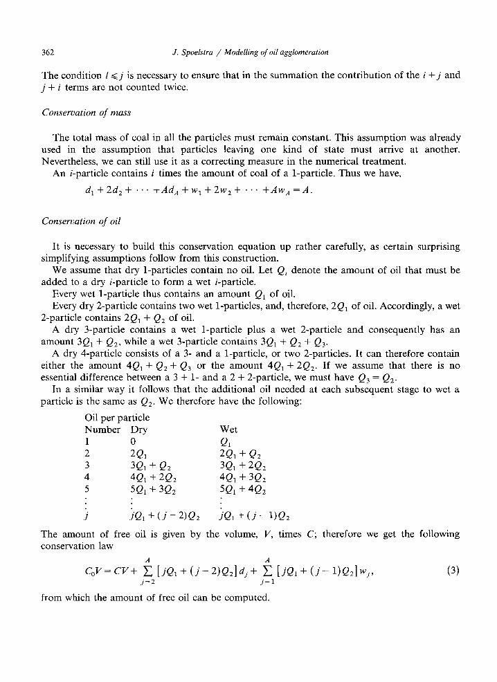
We assume that dry l-particles contain no oil. Let Qi denote the amount of oil that must be added to a dry i-particle to form a wet i-particle.

Every wet l-particle thus contains an amount Q, of oil. Every dry 2-particle contains two wet l-particles, and, therefore, 2Q, of oil. Accordingly, a wet

2-particle contains 2Qi + Q2 of oil. A dry 3-particle contains a wet l-particle plus a wet 2-particle and consequently has an

amount 3Qi + Q2, while a wet 3-particle contains 3Qi + Q2 + Q3. A dry 4-particle consists of a 3- and a l-particle, or two 2-particles. It can therefore contain

either the amount 4Qi + Q2 + Q3 or the amount 4Qi + 2Q2. If we assume that there is no essential difference between a 3 + l- and a 2 + 2-particle, we must have Q3 = Q2.

In a similar way it follows that the additional oil needed at each subsequent stage to wet a particle is the same as Q2. We therefore have the following:

Oil per particle Number Dry Wet 1 0 Q, 2 2Ql 2Q1+ Qz 3 3Q1+ Qz 3Q1+ 2Q2 4 4Q1-t 2Q2 4Ql+ 3Qz 5 5Q1+ 3Q2 5Q1+ 4Qz

j ~Ql+(j-2)Q2 jQl + (j - 1)Q2

The amount of free oil is given by the volume, I’, times C; therefore we get the following conservation law

CP=Cv+ 6 [jQl+(j-2)Q2]dj+ ? [jQl+(j-l)Q21wjy j=2 j=l

from which the amount of free oil can be computed.

(3)


The model thus consists of the system of 2A equations (1) and (2) and the conservation equation (3) in the 2A + 1 unknown functions d,, . . . , dA, wl,. . . , wA and C. These equations contain the A + A2 + 2 parameters g,, . . . , g,, k,,, i, j = 1,. . . , A, Q, and Q2.

In the following section we discuss ways of reducing the number of parameters and a method of solving the equations.

4. Solving the model

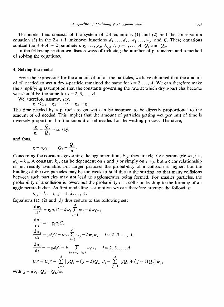
From the expressions for the amount of oil on the particles, we have obtained that the amount of oil needed to wet a dry i-particle remained the same for i = 2,. . . , A. We can therefore make the simplifying assumption that the constants governing the rate at which dry i-particles become wet should be the same for i = 2, 3,. . . , A.

We, therefore assume, say, g,<g,=g,= *** =g,=g.

The time needed by a particle to get wet can be assumed to be directly proportional to the amount of oil needed. This implies that the amount of particles getting wet per unit of time is inversely proportional to the amount of oil needed for the wetting process. Therefore,

g - !ZfL = (y say --

g1 Q2 ’ ’

and thus,

g= Ql, Q,=+

Concerning the constants governing the agglomeration, k,,, they are clearly a symmetric set, i.e., kij = kji. A constant kij can be dependent on i and j or simply on i +j, but a clear relationship is not readily available. For larger particles the probability of a collision is higher, but the binding of the two particles may be too weak to hold due to the stirring, so that many collisions between such particles may not lead to agglomerates being formed. For smaller particles, the probability of a collision is lower, but the probability of a collision leading to the forming of an agglomerate higher. As first modelling assumption we can therefore attempt the following:

kij=k, i, j=l,2 ,..., A.

Equations (l), (2) and (3) thus reduce to the following set:

d w, A

- = g,d,C - kw, c wj - kwlwl, dt j=l

dd, - = -g,d,C,

dt

dw,

dt = gdiC - kwi 6 wj - kwiwi, i=2,3 > . . . > A,

j=l

Cv= C,v- C [jQl + (_i_2)Qz]dj- C j=2 j=l

[jQl + (j - l)Q2IWj,

ddi

dt - -gd,C+k c w[wj9 i = 2, 3,

/+j=i, /Cj

A A

. . . . A,

with g = agl, Q2 = Q,/a.


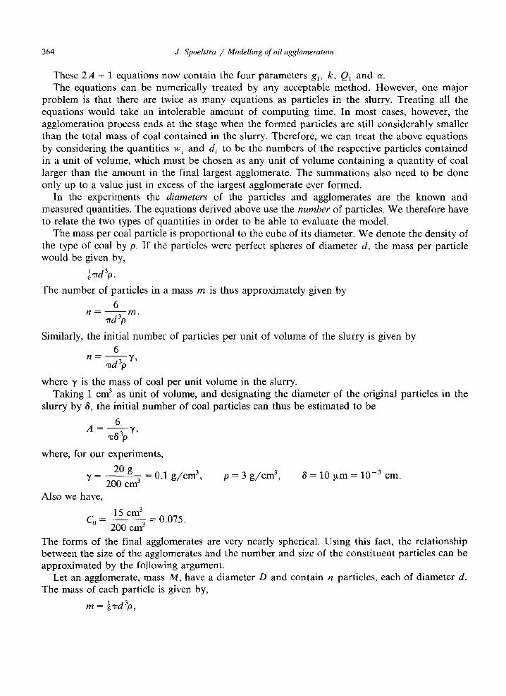
These 2A + 1 equations now contain the four parameters g,, k, Qi and (Y. The equations can be numerically treated by any acceptable method. However, one major

problem is that there are twice as many equations as particles in the slurry. Treating all the equations would take an intolerable amount of computing time. In most cases, however, the agglomeration process ends at the stage when the formed particles are still considerably smaller than the total mass of coal contained in the slurry. Therefore, we can treat the above equations by considering the quantities wi and di to be the numbers of the respective particles contained in a unit of volume, which must be chosen as any unit of volume containing a quantity of coal larger than the amount in the final largest agglomerate. The summations also need to be done only up to a value just in excess of the largest agglomerate ever formed.

In the experiments the diameters of the particles and agglomerates are the known and measured quantities. The equations derived above use the number of particles. We therefore have to relate the two types of quantities in order to be able to evaluate the model.

The mass per coal particle is proportional to the cube of its diameter. We denote the density of the type of coal by p. If the would be given by,

+=d3p.

The number of particles in a

6 n=-m.

,rrd3p

particles were perfect spheres of diameter d, the mass per particle

mass m is thus approximately given by

Similarly, the initial number of particles per unit of volume of the slurry is given by

6 n=-y,

Td3p

where y is the mass of coal per unit volume in the slurry. Taking 1 cm3 as unit of volume, and designating the diameter of the original particles in the

slurry by 6, the initial number of coal particles can thus be estimated to be

6 A=-y,

7TS3p

where, for our experiments,

20 Y= g = = 200 cm3

0.1 g/cm3, p 3 g/cm3, 6 = 10 pm = lop3 cm.

Also we have,

c = 15 cm3 0

200 cm3 = 0.075.

The forms of the final agglomerates are very nearly spherical. Using this fact, the relationship between the size of the agglomerates and the number and size of the constituent particles can be approximated by the following argument.

Let an agglomerate, mass M, have a diameter D and contain n particles, each of diameter d. The mass of each particle is given by,

m = &d3p,


while the mass of the agglomerate is given by,

M=nm.

But, ignoring the oil and spaces between particles, it is also approximately given by

A4 = +7D3p.

Thus D3 = nd3 or, D = n’13d and consequently the diameter of an i-particle can be approximated by

D. = n?13g I 1.

5. Numerical results and conclusions

In solving the equations we used Euler’s method and a Runge-Kutta method of order 4. In both methods we started with a step size of 0.01 along the time axis, which was increased by 5% following each step. Experimental data were available at 60 s, 120 s,. . . ,300 s as in the first column of Table 1. Due to the 5% increases in the time steps, these instants of time would normally not be reached exactly. The step size therefore had to be adjusted near these instants in order to obtain the prediction of the model for the organic recovery at those moments. The time step was then readjusted to 0.4 and allowed to increase by 5% per step once again. In the Euler method the step size was never allowed to exceed 0.5. No such bound was placed on the step size for the Runge-Kutta method, as the adjustments mentioned above restricted the step size sufficiently.

Parameters in the model characterizing the experiments, were computed in the same way as discussed fully by Spoelstra and van Wyk [5]. We considered the sum of the squares of the differences between experimental data and predictions of the model, called the sum of the

Table 1 Correspondence between model and an experiment

Parameters

g1

1.426

k

2.697.10F6

PI (Y

2.620.10-l’ 0.8443

Time (s) Organic Recovery

0 60

120 150 180 200 240 300

* Experimental value unreliable.

Experimental Predicted

0 0.0

* 0.1

56 55.6

63 76.7

95 85.4 100 88.6 100 92.3

100 95.0


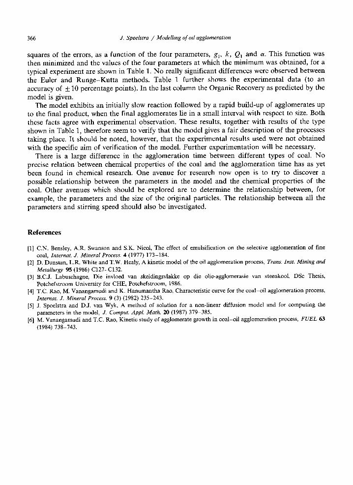
squares of the errors, as a function of the four parameters, g,, k, Q, and (Y. This function was then minimized and the values of the four parameters at which the minimum was obtained, for a typical experiment are shown in Table 1. No really significant differences were observed between the Euler and Runge-Kutta methods. Table 1 further shows the experimental data (to an accuracy of + 10 percentage points). In the last column the Organic Recovery as predicted by the model is given.

The model exhibits an initially slow reaction followed by a rapid build-up of agglomerates up to the final product, when the final agglomerates lie in a small interval with respect to size. Both these facts agree with experimental observation. These results, together with results of the type shown in Table 1, therefore seem to verify that the model gives a fair description of the processes taking place. It should be noted, however, that the experimental results used were not obtained with the specific aim of verification of the model. Further experimentation will be necessary.

There is a large difference in the agglomeration time between different types of coal. No precise relation between chemical properties of the coal and the agglomeration time has as yet been found in chemical research. One avenue for research now open is to try to discover a possible relationship between the parameters in the model and the chemical properties of the coal. Other avenues which should be explored are to determine the relationship between, for example, the parameters and the size of the original particles. The relationship between all the parameters and stirring speed should also be investigated.

References

[l] C.N. Bensley, A.R. Swanson and SK. Nicol, The effect of emulsification on the selective agglomeration of fine coal, Znternat. J. Mineral Process. 4 (1977) 173-184.

[2] D. Dunstan, L.R. White and T.W. Healy, A kinetic model of the oil agglomeration process, Trans. Inst. Mining and

Metallurgy 95 (1986) C127-C132.

[3] B.C.J. Labuschagne, Die invloed van skeidingsvlakke op die olie-agglomerasie van steenkool, DSc Thesis, Potchefstroom University for CHE, Potchefstroom, 1986.

[4] T.C. Rao, M. Vanangamudi and K. Hanumantha Rao, Characteristic curve for the coal-oil agglomeration process, Znternat. J. Mineral Process. 9 (3) (1982) 235-243.

[5] J. Spoelstra and D.J. van Wyk, A method of solution for a non-linear diffusion model and for computing the parameters in the model, J. Comput. Appl. Math. 20 (1987) 379-385.

[6] M. Vanangamudi and T.C. Rao, Kinetic study of agglomerate growth in coal-oil agglomeration process, FUEL 63

(1984) 738-743.

the modelling of oil agglomeration of coal fines

Documents