The Mismatch Between Life Insurance Holdings and Financial Vulnerabilities:Evidence from the Health and Retirement Survey

by

B. Douglas BernheimStanford University and

National Bureau of Economic Researchbernheim@leland.stanford.edu

Lorenzo ForniBoston University and

Bank of Italylforni@bu.edu

Jagadeesh GokhaleFederal Reserve Bank of Cleveland

ajgokhale@stratos.net

Laurence J. KotlikoffBoston University and

National Bureau of Economic Researchkotlikof@bu.edu

January 2001

__________________________We are grateful to two referees and seminar participants at the National Bureau of Economic Researchfor helpful comments, and to Neva Kerbeshian and Noshua Watson for able research assistance. TheNational Institute of Aging provided financial support. Economic Security Planner (ESPlanner) is used inthis study with the permission of Economic Security Planning, Inc.

Abstract

Using data on older workers from the 1992 Health and Retirement Survey along with an elaborate life-cycleplanning model, we quantify the extent to which the death of each individual would affect the financial statusof his or her survivors, and we measure the degree to which life insurance holdings moderate theseconsequences. The average change in living standard that would result from a spouse’s death is small bothin absolute terms and relative to the decline that would occur in the absence of insurance. However, thisaverage obscures a startling mismatch between insurance holdings and underlying vulnerabilities. For manyof those with the greatest vulnerabilities, the amounts purchased are surprisingly small, and for many of thosewith the smallest vulnerabilities, the amounts are surprisingly large. As a result, uninsured vulnerabilities arereasonably widespread. The magnitude of these vulnerabilities, as well as the proclivity to address any givendegree of vulnerability by purchasing life insurance, vary systematically with individual and householdcharacteristics.

1Social security earnings histories are contained in a matched, supplemental data set, which we have usedin compliance with confidentiality requirements and security restrictions.

2The model is embodied in financial planning software, Economic Security Planner (or ESPlanner), whichwas co-developed by three of this paper’s authors. Economic Security Planning, Inc. provides free copies of the

1

1. Introduction

The purpose of this study is to examine life insurance holdings and financial vulnerabilities among

couples approaching retirement age. Two separate concerns motivate our analysis. First, there are reasons

to suspect that life insurance coverage may be poorly correlated with underlying financial vulnerabilities. A

well-known insurance industry adage holds that life insurance is “sold and not bought.” Alternatively,

households may purchase long-term policies relatively early in life, and subsequently fail to adjust coverage

appropriately because of inertia and/or other psychological considerations. Second, households that purchase

little or no life insurance may leave either or both spouses at risk of serious financial consequences.

Past studies address the second issue, but provide little evidence concerning the first. Analyzing data

gathered during the 1960s from households in middle age through early retirement, Auerbach and Kotlikoff

[1987, 1991a, 1991b] found that roughly one-third of wives and secondary earners would have seen their

living standards decline by 25 percent or more had their spouses died. Holden, Burkhauser, and Myers [1986]

and Hurd and Wise [1989] documented sharp declines in living standards and increases in poverty rates (from

9 to 35 percent) among women whose husbands actually passed away.

This study builds on Auerbach and Kotlikoff’s work in four ways. First, we use recent, high quality

data drawn from the 1992 wave of the Health and Retirement Study (HRS). Second, we obtain more

accurate estimates of survival-contingent income streams through the use of actual social security earnings

histories and a highly detailed benefits calculator.1 Third, to evaluate the financial vulnerabilities of each

household, we employ an elaborate life-cycle model that accounts for a broad array of demographic,

economic, and financial factors not considered in previous research.2 These factors include household

software for academic research. For additional information, consult www.ESPlanner.com.

2

composition, economies of shared living, liquidity constraints, inflexible expenses, and various details of state

and federal tax codes. Fourth, we quantify the financial vulnerabilities that would have existed in the absence

of insurance, and evaluate the extent to which life insurance holdings addressed those vulnerabilities,

particularly for cases in which the potential financial consequences of a spouse’s death were severe.

Throughout our analysis, we adopt a concrete and easily understood yardstick for quantifying financial

vulnerabilities: the percentage decline in an individual’s sustainable living standard that would result from a

spouse’s death. The use of this yardstick permits us to make apples-to-apples comparisons of vulnerabilities

across households, and to investigate correlations between vulnerabilities and insurance coverage. We also

compare actual life insurance holdings to a natural benchmark, defined as the level of coverage required to

assure survivors of no change in their sustainable living standard. It is worth emphasizing that we do not

regard this benchmark as a definitive standard of adequacy or rationality. Rational decision makers may elect

to purchase either higher or lower levels of insurance. However, when combined with other evidence on

household objectives, comparisons with the benchmark potentially shed light on the adequacy of life insurance

coverage.

Averaged across our entire sample, the change in living standard that would result from a spouse’s

death is small both in absolute terms and relative to the average decline that would have occurred in the

absence of insurance (henceforth referred to as the underlying vulnerability). However, this average

obscures a startling mismatch between life insurance holdings and underlying vulnerabilities. Many older

workers required little or no insurance to ensure survivors of undiminished living standards, yet nevertheless

maintained substantial coverage. Relative to earnings, individuals with greater underlying vulnerabilities did

not, on average, purchase more life insurance. Moreover, the likelihood of having no life insurance protection

was greatest for those with the largest exposures. On the margin, life insurance offset only ten percent of

3

the variation in financial vulnerability across all individuals, and virtually none of the variation in financial

vulnerability across individuals at risk of reduced living standards. Consequently, among those with serious

financial vulnerabilities, differences between benchmark and actual levels of life insurance were substantial.

Ignoring life insurance, 33 percent of secondary earners and 6 percent of primary earners would have

experienced significant (20 percent or greater) declines in living standards had their spouses died in 1992; 20

percent of secondary earners and 3 percent of primary earners would have experienced severe (40 percent

or greater) declines. Only one in three households in these at-risk populations held sufficient life insurance

to avert significant or severe financial consequences for surviving secondary earners; for at-risk primary

earners, the figure is less than one in six. The magnitude of uninsured financial vulnerabilities, as well as the

proclivity to address any given degree of vulnerability by purchasing life insurance, varies systematically with

individual and household characteristics.

The paper proceeds as follows: section 2 discusses methods, section 3 describes the data, section 4

presents basic results, section 5 provides sensitivity analysis, and section 6 concludes.

2. A Strategy for Measuring Financial Vulnerabilities

A. Concepts

We clarify our strategy for measuring financial vulnerabilities through an example. Imagine that a

husband and wife each live for at most two years (equivalently, they are within two years of maximum

lifespan). Both are alive initially, but either may die before the second year. The household’s well-being

depends on consumption in each year and survival contingency. As discussed further below, we allow for

the possibility that some ongoing expenditures are either exogenous or determined early in life by “sticky”

choices. We refer to these expenditures as “fixed consumption,” and to residual spending as “variable

consumption.” Let y1 denote initial assets plus first period earnings net of fixed consumption, and let y2s

4

(1)

(2)

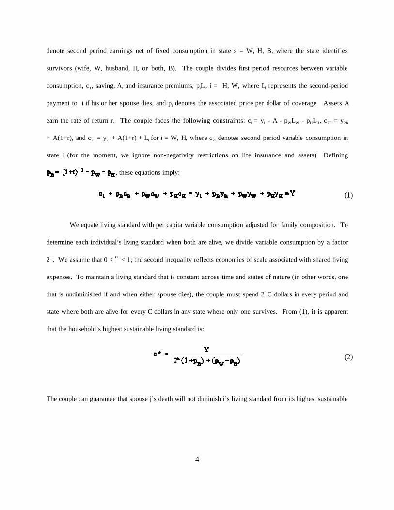
denote second period earnings net of fixed consumption in state s = W, H, B, where the state identifies

survivors (wife, W, husband, H, or both, B). The couple divides first period resources between variable

consumption, c1, saving, A, and insurance premiums, piLi, i = H, W, where Li represents the second-period

payment to i if his or her spouse dies, and pi denotes the associated price per dollar of coverage. Assets A

earn the rate of return r. The couple faces the following constraints: c1 = y1 - A - pWLW - pHLH, c2B = y2B

+ A(1+r), and c2i = y2i + A(1+r) + Li for i = W, H, where c2i denotes second period variable consumption in

state i (for the moment, we ignore non-negativity restrictions on life insurance and assets) Defining

, these equations imply:

We equate living standard with per capita variable consumption adjusted for family composition. To

determine each individual’s living standard when both are alive, we divide variable consumption by a factor

2". We assume that 0 < " < 1; the second inequality reflects economies of scale associated with shared living

expenses. To maintain a living standard that is constant across time and states of nature (in other words, one

that is undiminished if and when either spouse dies), the couple must spend 2"C dollars in every period and

state where both are alive for every C dollars in any state where only one survives. From (1), it is apparent

that the household’s highest sustainable living standard is:

The couple can guarantee that spouse j’s death will not diminish i’s living standard from its highest sustainable

3In the special case where the household has Leontief preferences (defined over per capita adjustedexpenditures), this is also the utility maximizing outcome.

4Note that, when actual life insurance is below the benchmark, the intact couple saves on insurancepremiums, so its actual consumption exceeds c*. Hence, the IMPACT variables understate the change in livingstandard that an individual experiences upon a spouse’s death. However, since life insurance premiums typicallyaccount for a small fraction of expenditures, the degree of understatement is small.

5A non-negativity constraint for life insurance purchases is equivalent to the restriction that life annuitiesare not available for purchase at the margin. For further discussion, see Yaari (1965), Kotlikoff and Spivak (1981), andBernheim (1987).

5

level, c*, by purchasing a life insurance policy with face value .3

We measure underlying financial vulnerabilities by comparing an individual’s highest sustainable living

standard, c*, with , which represents the living standard he or she would enjoy if widowed,

ignoring life insurance. We define the variable IMPACT (ignoring insurance) as , i = W,H.

This is a measure of the percent by which the survivor’s actual living standard would, with no insurance

protection, fall short of or exceed the couple’s highest sustainable living standard. Similarly, we measure

uninsured financial vulnerabilities by comparing c* with , which represents the living

standard that the individual would actually enjoy if widowed, based on actual life insurance coverage, .

We define the variable IMPACT (actual) as . This is a measure of the percent by which

the survivor’s actual living standard would, given actual levels of coverage, fall short of or exceed the

couple’s highest sustainable living standard. The IMPACT variables are based on a concrete and easily

understood yardstick for quantifying the consequences of a spouse’s death.4 We also compare actual life

insurance holdings, , with the benchmark level, .

For the preceding example, we implicitly assumed that individuals could borrow at the rate r and issue

survival-contingent claims at the prices pH and pW. As a practical matter, households encounter liquidity

constraints and are typically unable to purchase negative quantities of (i.e. sell) life insurance.5 In solving for

each household’s highest sustainable living standard, we take these restrictions into account, smoothing

6Formally, one can think of the outcome that we identify as the limit of the solutions to a series of utilitymaximization problems in which the intertemporal elasticity of substitution approaches zero. In the limit (the Leontiefcase), the household is actually indifferent with respect to the distribution of consumption across any years in whichits living standard exceeds the minimum level.

6

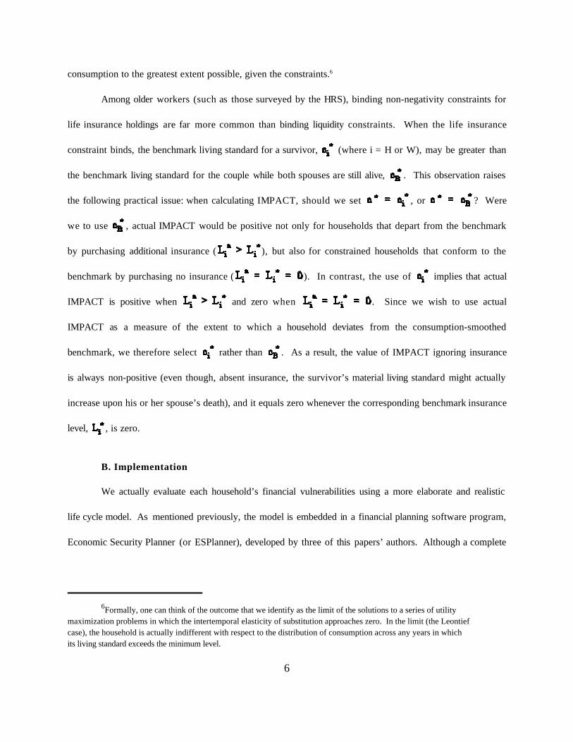
consumption to the greatest extent possible, given the constraints.6

Among older workers (such as those surveyed by the HRS), binding non-negativity constraints for

life insurance holdings are far more common than binding liquidity constraints. When the life insurance

constraint binds, the benchmark living standard for a survivor, (where i = H or W), may be greater than

the benchmark living standard for the couple while both spouses are still alive, . This observation raises

the following practical issue: when calculating IMPACT, should we set , or ? Were

we to use , actual IMPACT would be positive not only for households that depart from the benchmark

by purchasing additional insurance ( ), but also for constrained households that conform to the

benchmark by purchasing no insurance ( ). In contrast, the use of implies that actual

IMPACT is positive when and zero when . Since we wish to use actual

IMPACT as a measure of the extent to which a household deviates from the consumption-smoothed

benchmark, we therefore select rather than . As a result, the value of IMPACT ignoring insurance

is always non-positive (even though, absent insurance, the survivor’s material living standard might actually

increase upon his or her spouse’s death), and it equals zero whenever the corresponding benchmark insurance

level, , is zero.

B. Implementation

We actually evaluate each household’s financial vulnerabilities using a more elaborate and realistic

life cycle model. As mentioned previously, the model is embedded in a financial planning software program,

Economic Security Planner (or ESPlanner), developed by three of this papers’ authors. Although a complete

7The software has many capabilities that we do not make use of here due to data limitations. For example, itcan account for a variety of special expenditures (college education, weddings, etc.), plans to change homes,various kinds of state contingent plans (e.g. a non-working wife plans to return to work and spend less on a child’seducation if her husband dies), and estate plans (including intended bequests).

8Our child-adult equivalency factor is that used by the OECD (see Ringen, 1991). Nelson’s (1992) worksuggests a smaller value, but she considers total household expenditures whereas our child-adult equivalency factorapplies only to non-housing consumption expenditure; for our base-case results, we treat housing expenditure asinflexible. It appears from Nelson’s work that a higher equivalency factor is appropriate for non-housingexpenditures.

9The OECD uses a value of 0.7 for " (see Ringen, 1991). Williams, et. al. (1998) consider values of 0.5 forboth " and $.

7

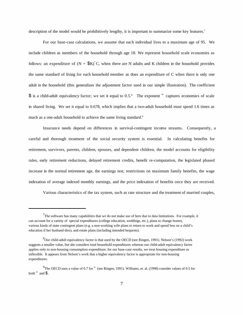
description of the model would be prohibitively lengthy, it is important to summarize some key features.7

For our base-case calculations, we assume that each individual lives to a maximum age of 95. We

include children as members of the household through age 18. We represent household scale economies as

follows: an expenditure of (N + $K)"C, when there are N adults and K children in the household provides

the same standard of living for each household member as does an expenditure of C when there is only one

adult in the household (this generalizes the adjustment factor used in our simple illustration). The coefficient

$ is a child-adult equivalency factor; we set it equal to 0.5.8 The exponent " captures economies of scale

in shared living. We set it equal to 0.678, which implies that a two-adult household must spend 1.6 times as

much as a one-adult household to achieve the same living standard.9

Insurance needs depend on differences in survival-contingent income streams. Consequently, a

careful and thorough treatment of the social security system is essential. In calculating benefits for

retirement, survivors, parents, children, spouses, and dependent children, the model accounts for eligibility

rules, early retirement reductions, delayed retirement credits, benefit re-computation, the legislated phased

increase in the normal retirement age, the earnings test, restrictions on maximum family benefits, the wage

indexation of average indexed monthly earnings, and the price indexation of benefits once they are received.

Various characteristics of the tax system, such as rate structure and the treatment of married couples,

10More specifically, 5,753 said that they planned to stay in their current home after retirement, 180 said thatthe expected to divide time between their current home and another location, 2,192 said that they planned to move,41 said that they had already moved, and 679 said that they don’t know. In addition, 3,705 households were notasked the question (mainly because they had already retired), and 102 households were asked but did not answer.

8

can alter insurance needs by influencing the distribution of after-tax income across the various survival

contingencies. Consequently, a careful treatment of taxation is also critical. The model calculates federal

and state income and payroll taxes for each year in each survival contingency. It incorporates wide range

of provisions, including federal deductions and exemptions, the decision to itemize deductions, the taxation of

social security benefits, the earned income tax credit, the child tax credit, the phase-out at higher income

levels of itemized deductions, and the indexation of tax brackets to the consumer price index. In computing

federal deductions, it determines whether the sum of state income taxes, mortgage interest payments, and

property taxes is large enough to justify itemization. Contributions to tax-favored retirement savings accounts

are excluded from taxable income, and withdrawals are included. Though the model determines total saving

simultaneously with life insurance, tax-favored saving is specified exogenously.

Choices concerning housing may also affect life insurance needs. Unlike many other expenditures,

housing outlays are not easily smoothed. It is difficult to scale mortgage, property tax, and insurance

payments up and down with other expenditures. Cost and inconvenience discourage many households from

moving or refinancing mortgages; others form psychological attachments to their homes, and resist changing

residences prior to death (Venti and Wise, 2000). For the HRS sample, roughly three quarters of respondents

reported that they planned to remain in their current home after retirement.10 Moreover, few households

access the equity in their homes through refinancing or reverse annuity mortgages (Caplin, 2000).

Consequently, for our base-case calculations, we treat housing as fixed consumption. In effect, we assume

that couples and survivors remain in the same home until death, and die with home equity intact. Formally,

we subtract housing expenses from income off-the-top, itemizing mortgage interest and property taxes as

11See Lundberg (1999) for a discussion.

12For additional examples, and for comparisons with recommendations generated by Quicken FinancialPlanner, see Gokhale, Kotlikoff, and Warshawsky (1999).

9

deductions for federal income tax purposes when it is optimal to do so, prior to smoothing variable

consumption.

Several potentially important factors are omitted from our analysis. We do not model uncertainty

concerning future income and non-discretionary expenses (e.g. medical care). Since small groups of

individuals can share risks to some extent, the adverse effect of uncertainty on living standard is probably

greater for widows and widowers than for couples. For this reason, our analysis tends to understate

insurance needs. We also neglect the possibility that an individual might remarry after a spouse’s death. The

extent to which remarriage mitigates the financial consequences of a spouse’s death depends on one’s view

of the marriage market.11 In any case, remarriage is relatively uncommon for the age group we consider (see

section 5).

Table 1 summarizes some illustrative life insurance calculations.12 We begin with a couple consisting

of a 54 year-old man earning $45,000 per year, and a 50 year-old woman earning $25,000 per year. The man

intends to retire at age 64, the woman at age 63. They have one 18 year old child. The net value of their

non-housing assets is $50,000; in addition, they own a $100,000 home, and have an unpaid mortgage balance

of $20,000. They expect their real earnings to grow at the rate of one percent per year until retirement. They

also expect to earn a real after-tax return of 3 percent on their non-housing investments. According to our

model, this couple must purchase $133,500 in term insurance on the husband’s life, and no insurance on the

wife’s life, to ensure each potential survivor of an undiminished living standard. The remainder of the table

illustrates the sensitivity of insurance needs to changes in various household characteristics and economic

parameters.

10

C. Interpretation

We do not regard our IMPACT variables as perfect measures of financial vulnerability. Though

elaborate, the life cycle model used in our analysis is still an abstraction, and we have imperfect information

concerning the economic circumstances of each household (see the Appendix). Nor do we regard the

benchmark level of life insurance as an objective standard of adequacy or rationality. Optimal insurance

coverage depends on a variety of considerations, including (but not limited to) the manner in which marginal

utilities vary across survival states, the weights that households attach to the well-being of each family

member, degrees of risk aversion, and load factors (more generally, the degree to which the industry departs

from actuarially fair pricing). Consequently, it is possible to rationalize a wide range of behaviors.

Nevertheless, the absence of a significant correlation between life insurance and financial

vulnerabilities (measured by IMPACT, ignoring insurance) would be difficult to reconcile with theories of

rational financial behavior. Even if a household places less weight on the well-being of a particular spouse,

and even if it must pay actuarially unfair rates, it should still obtain greater insurance protection when the

spouse in question is exposed to more severe financial consequences. To explain the absence of a correlation,

one would need to believe either that our measure of IMPACT (ignoring insurance) is largely unrelated to

underlying vulnerabilities, or that marginal utilities vary in a way that just offsets the differences in measured

vulnerabilities. Both possibilities strike us as improbable.

Evidence of widespread and substantial uninsured vulnerabilities (as measured by actual IMPACT

or by the divergence of actual insurance from the benchmark) would also be more difficult to rationalize than

it might at first appear. Most potential explanations presuppose that households deliberately choose different

living standards for survivors. Yet this premise is inconsistent with preliminary findings from a financial

planning case study at Boston University, involving (to date) more than 300 subjects. Each of these

individuals constructed a comprehensive financial plan using the same financial planning software employed

13Even with risk aversion, such choices are reasonable if load factors are low. For evidence on load factorsin the context of life annuities, see Mitchell, Poterba, Warshawsky, and Brown (1999).

14 The HRS sampled 5,000 married couples in which both spouses responded, 200 married couples in which

one spouse refused to answer, and 2,452 single individuals.

15 Mitchell and Moore (1997a and 1997b) provide excellent descriptions of the HRS, in general, and the

wealth accumulation of the HRS sample in particular.

11

in the current study. Participants hoped to benefit from these sessions, and therefore had strong incentives

to provide accurate information. Though the software permits users to specify different living standards for

intact couples and each potential survivor, every subject selected the same living standard for each

contingency.13 While it is perfectly rational for individuals to have other objectives, it is irrational for

individuals with these objectives to purchase coverage that diverges significantly from our benchmark

(assuming, of course, that the benchmark is derived from a model that correctly depicts all important aspects

of the household’s opportunity set).

3. Data

The 1992 wave of the HRS (fielded between April 1992 and March 1993) surveyed over 7000

households with at least one spouse between the ages of 51 and 61.14 The data cover health status, income,

wealth, pensions, social security benefits, demographics, education, housing, food consumption, family

structure and transfers, current and past employment, retirement plans, cognition, health and life insurance,

intra vivos gifts, inheritances, and bequests.15 Despite the survey’s thoroughness, it was necessary to impute

a number of household characteristics; see the Appendix for details.

Our final sample consists of 2,113 couples. Table 2 provides some descriptive statistics. We

excluded couples for the following reasons: a) Social Security earnings records were unavailable for either

spouse; b) a spouse provided inadequate information concerning life insurance policies; c) a spouse refused

to be interviewed; d) a spouse was unemployed; or e) the couple’s reported income and other economic

12

resources were insufficient to support its reported fixed expenditures. Criterion (a) accounted for nearly 80

percent of excluded observations, and criterion (b) accounted for most of the remaining exclusions.

4. Results

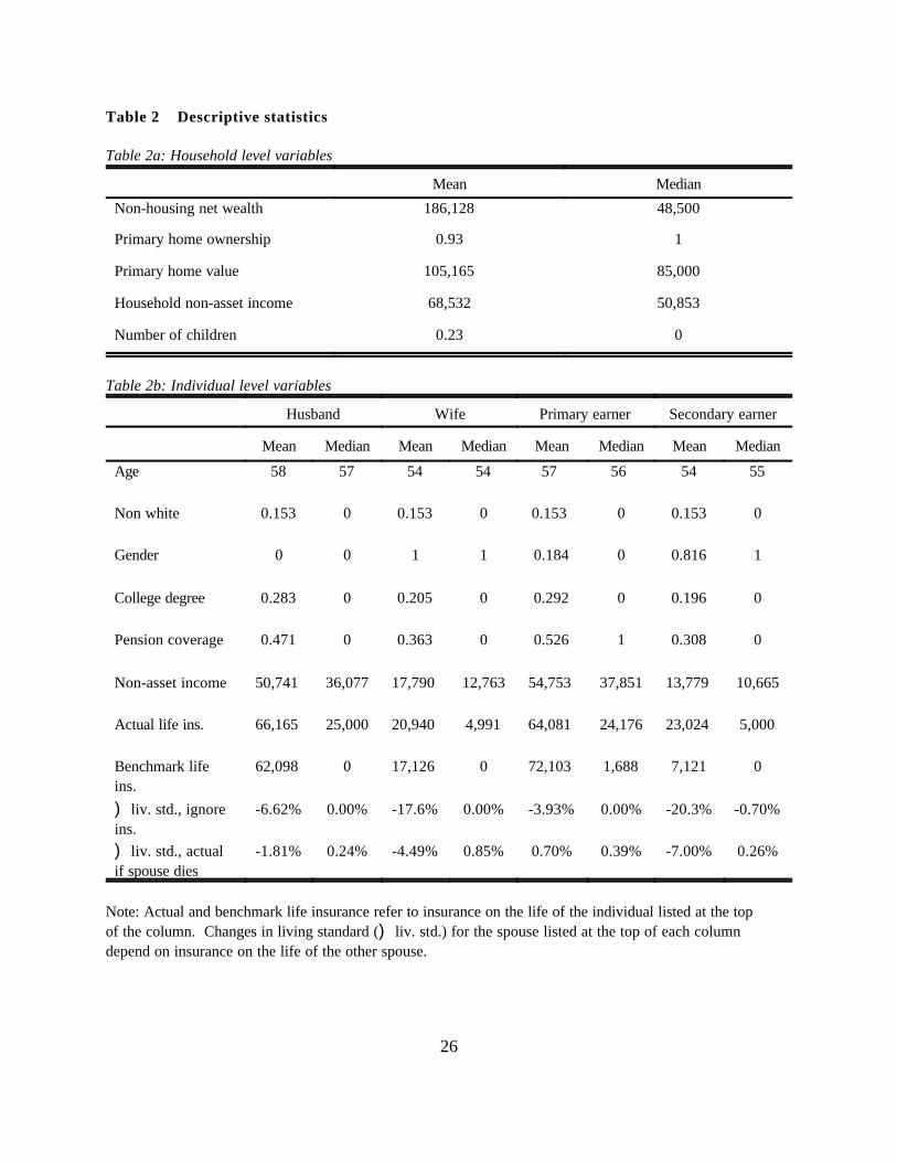
According to table 2, average actual life insurance holdings were close to average benchmark levels

for husbands and wives. The average benchmark exceeded the average level of insurance on the life of a

primary earner by $8,022 (a rather small sum when amortized over the individual’s remaining lifespan); for

secondary earners, this relation was reversed. In each case, median life insurance surpassed the median

benchmark.

In the second-to-last line of table 2b () liv. std., ignore ins.), we tabulate means and medians for

IMPACT calculated as if each household held no life insurance. This variable measures underlying financial

exposure. Without insurance, the average living standards for surviving husbands, wives, primary earners,

and secondary earners would have been, respectively, 6.6 percent, 17.6 percent, 3.9 percent, and 20.3 percent

below their highest sustainable levels. Since the corresponding medians for husbands, wives, and primary

earners are zero, we can infer that more than half of these individuals were not at-risk of a reduction in

sustainable living standard. This finding reflects the fact that many older workers have relatively little human

capital to protect.

In the final line of table 2b () liv. std., actual), we tabulate means and medians for IMPACT based

on actual insurance holdings. This variable measures residual (uninsured) financial exposure. For both

husbands and wives, life insurance reduced average IMPACT by nearly 75 percent. The proportional effect

is somewhat smaller for surviving secondary earners, who would, on average, have seen their living standards

decline by 7 percent. Accounting for life insurance, a surviving primary earner would not, on average, have

experienced any decline in living standard.

13

Based on these initial findings, one might be inclined to conclude that households with older workers

generally carry sufficient insurance to protect survivors against significant declines in living standards.

However, this conclusion is premature. Underlying financial exposures vary dramatically across households.

From an inspection of averages (table 2), one cannot determine whether the distribution of insurance holdings

matches up with the distribution of exposures.

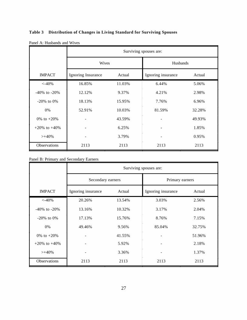
Table 3 provides further information on the distributions of both IMPACT variables. As discussed

previously, ignoring insurance, IMPACT is never strictly greater than zero. This reflects the fact that we

have imposed a non-negativity constraint on life insurance purchases. An individual’s living standard may

rise upon a spouse’s death; however, without life insurance, it cannot exceed the living standard that the he

or she would enjoy as a survivor assuming implementation of the (constrained) benchmark financial plan.

Note also that actual IMPACT is exactly equal to zero for a substantial fraction of the population. Generally,

these are individuals for whom actual and (model-generated) benchmark levels of insurance protection are

both zero.

It is readily evident that insurance holdings match up poorly with financial vulnerabilities. Only 47.1

percent of wives, 18.4 percent of husbands, 50.5 percent of secondary earners, and 15.0 percent of primary

earners in the HRS sample required insurance protection to avoid reductions in sustainable living standards

upon their spouses’ deaths (in Table 3, those with IMPACT, ignoring insurance, less than zero). In contrast,

life insurance actually protected 78.7 percent of wives, 61.2 percent of husbands, 77.9 percent of secondary

earners, and 62.1 percent of primary earners. Overall, 53.6 percent of wives, 52.7 percent of husbands, 50.8

percent of secondary earners, and 55.5 percent of primary earners had strictly positive life insurance

protection despite the fact that they would have experienced increases in living standards upon the deaths of

their spouses (in Table 3, those with actual IMPACT greater than zero).

If life insurance holdings were sufficient on average to avert significant declines in survivors’ living

14

standards, and if a significant portion of this coverage “protected” individuals without serious exposures, then

many of those at-risk must have had substantial uninsured vulnerabilities. According to table 3, insurance

reduced the fraction of individuals at-risk of severe financial consequences (defined as a decline in living

standard of 40 percent or greater) from 16.9 percent to 11.0 percent for wives, from 20.3 percent to 13.5

percent of secondary earners, from 6.4 percent to 5.1 percent of husbands, and from 3.0 percent to 2.6

percent for primary earners. Similarly, insurance reduced the fraction of individuals at-risk of significant

financial consequences (defined as a decline in living standard of 20 percent or greater) from 29.0 percent

to 20.4 percent for wives, from 33.4 percent to 23.9 percent for secondary earners, from 10.7 percent to 8.0

percent for husbands, and from 6.2 percent to 4.6 percent for primary earners. Roughly speaking, only 25

to 30 percent of households with significant financial exposures held sufficient life insurance to avert

significant consequences for survivors.

Thus far, we have measured the consequences of a spouse’s death in terms of the proportional

change in sustainable living standard. For many individuals, the potential financial consequences of a spouse’s

death are also severe in absolute terms. Prior to the death of either spouse, sustainable consumption for 8.0

percent of the couples in our sample fell below the 1992 poverty thresholds published by the U.S. Census

Bureau. Taking into account actual levels of insurance coverage, poverty rates would have been 22.5 percent

among surviving wives and 14.6 percent among surviving husbands. These findings imply that 64 percent

(14.5 of 22.5 percentage points) of poverty among surviving women and nearly 45 percent (6.6 out of 14.6

percentage points) of poverty among surviving men resulted from a failure to ensure survivors of an

undiminished living standard through insurance. Ignoring insurance, poverty rates would have been 27.6

percent among surviving wives and 16.0 percent among surviving husbands. Consequently, insurance

eliminated only 26 percent of the avoidable poverty among surviving widows (5.1 out of 19.6 percentage

points), and only 18 percent of the avoidable poverty among surviving men (1.4 out of 8.0 percentage points).

15

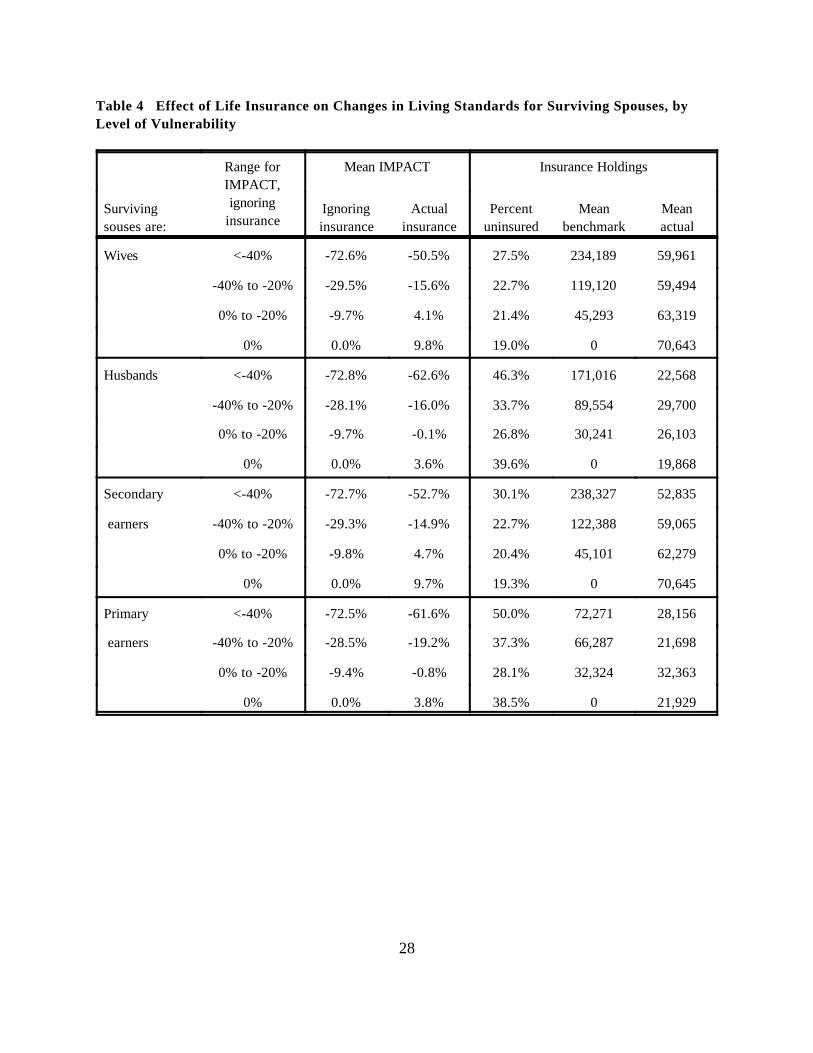
In table 4, we subdivide the population based on underlying financial exposure, measured by the value

of IMPACT, ignoring insurance. For each subgroup, we then calculate the means of both IMPACT

variables, as well as summary statistics describing insurance holdings. When we examine the data in this

way, it is even more apparent that insurance holdings are poorly correlated with financial vulnerabilities.

Note that the likelihood of having no life insurance protection was greatest for those with the largest

exposures. For secondary (primary) earners, 30.1 percent (50.0 percent) of those with severe exposures had

no insurance protection, compared with only 19.3 percent (38.5 percent) of those with no financial exposure.

In a simple probit regression explaining whether the couple held insurance on the primary earner’s life as a

function of IMPACT for the secondary earner (ignoring insurance), the slope coefficient was 0.00525 (F =

0.00097). For a similar probit regression explaining whether the couple held insurance on the secondary

earner’s life as a function of IMPACT for the primary earner (ignoring insurance), the slope coefficient was

0.00267 (F = 0.00194). In both instances, the positive coefficient indicates that those with lower

vulnerabilities are more likely to have insurance protection.

More generally, those with greater vulnerabilities did not, on average, have greater insurance

protection. According to table 4, the average level of protection for secondary earners falls monotonically

with the degree of underlying vulnerability, from $70,645 among those with no exposure, to only $52,835

among those with severe exposures. For primary earners, there is no obvious relation between average

insurance holdings and underlying vulnerabilities. For each observation, we computed the ratio of insurance

on the primary earner’s life to the primary earner’s annual wages, and regressed this on IMPACT for the

secondary earner (ignoring insurance). The slope coefficient was 0.0261 (F = 0.0095). In a similar

regression of the insurance-to-earnings ratio for the secondary earner on IMPACT for the primary earner

(ignoring insurance), the slope coefficient was 0.0491 (F = 0.0638). The positive coefficients indicate that

those with smaller vulnerabilities hold more insurance on average.

16For secondary earners, insurance reduced mean IMPACT by 22.1 percentage points (from -72.6 percent to-50.5 percent) among those with severe exposures, by 13.9 percentage points (from -29.5 percent to -15.6 percent)among those with IMPACT (ignoring insurance) between -20 percent and -40 percent, by 13.8 percentage points(from -9.7 percent to 4.1 percent) among those with IMPACT (ignoring insurance) between 0 percent and -20 percent,and by 9.8 percentage points (from 0.0 percent to 9.8 percent) among those with no exposure.

16

The difference between our two IMPACT variables (actual and ignoring insurance) provides another

measure of insurance coverage. If couples hold insurance to moderate the financial consequences of a

spouse’s death, then this difference should be larger for those with greater vulnerabilities. To some extent,

the statistics in table 4 confirm this prediction.16 However, the correlation is rather weak. In simple

regressions of IMPACT (actual insurance) on IMPACT (ignoring insurance), the coefficients of the latter

variable are 0.918 (F = 0.018) for primary earners, and 0.874 (F = 0.018) for secondary earners. In

analogous median regressions, the corresponding coefficients are 1.01 (0.018) for primary earners, and 1.01

(0.026) for secondary earners. The OLS regressions suggest that, on the margin, life insurance holdings

offset perhaps 10 percent of the variation in financial vulnerabilities, while the median regressions imply that

insurance coverage is entirely unrelated to the degree of financial vulnerability. Furthermore, when we

restrict attention to those for whom living standards would actually decline (absent insurance) upon a spouse’s

death, the corresponding OLS coefficients are 1.01 (F = 0.039) for primary earners, and 0.913 (F = 0.031)

for secondary earners, while the corresponding median regression coefficients are 1.04 (F = 0.009) for

primary earners, and 1.10 (F = 0.020) for secondary earners. Consequently, for those at-risk of some

reduction in living standard, insurance coverage bears very little relation to the degree of financial

vulnerability, and there is even some evidence that the correlation may be slightly negative (as indicated by

a coefficient in excess of unity).

We draw two other important conclusions from table 4. First, life insurance had, at best, a moderate

impact on financial exposures among the at-risk population. For example, among severely at-risk secondary

earners, insurance reduced the average consequences of a spouse’s death (mean IMPACT) by only thirty

17Formally, frac. addr. (fraction addressed) = [(Freq. Ins=0) - (Freq. Actual)]/(Freq. Ins=0).

17

percent, from -72.6 percent to -50.5 percent. This is a far cry from the three-fourths overall reduction in

mean IMPACT noted in table 2. For this same group, households would have needed to hold an average of

$234,189 to assure each surviving secondary earner of an undiminished living standard. In fact, they held on

average roughly one-quarter of this amount ($59,961). This implies a discrepancy far larger than the $8,022

overall difference noted in table 2.

Second, for a fixed level of financial exposure, households were more inclined to protect wives and

secondary earners than to protect husbands and primary earners. For example, among severely at-risk

individuals, only 27.5 percent of wives had no insurance protection, compared with 46.3 percent of husbands.

For severely at-risk wives, insurance reduced mean IMPACT by 22.1 percentage points (from -72.6 percent

to -50.5 percent), compared with only 10.2 percentage points (from -72.8 percent to -62.6 percent) for

husbands.

The frequencies of severe and significant uninsured financial exposures, implied by the distributions

of actual IMPACT in table 3, are lower than Auerbach and Kotlikoff’s estimates. Possible explanations for

the disparity include increases in female labor force participation since the 1960s, changes in patterns of

insurance coverage, and methodological differences.

Table 5 provides disaggregated results for various population subgroups. To conserve space, we

confine our attention to primary and secondary earners (results for husbands and wives are similar). In

addition to reporting the percentage of each subgroup with severe and significant exposures based on

IMPACT with actual insurance (Freq. Actual) and on IMPACT ignoring insurance (Freq. Ins=0), we also

report the fractional reduction in each exposure rate resulting from insurance coverage (Frac. Addr.).17

Significant and severe uninsured financial vulnerabilities were more common among low income

households, couples with disparate earnings, relatively young households, couples with dependent children,

18

and especially non-whites. As one would expect, the likelihood of having a substantial uninsured vulnerability

declines monotonically with the affected individual’s age. For secondary earners, the frequency of

vulnerability is non-monotonic in total household earnings; those belonging to middle income households are

least likely to experience significant or severe declines in living standard upon the primary earner’s death.

Households with combinations of risk factors may be particularly likely to have substantial uninsured

financial vulnerabilities. To investigate this possibility, we estimated quantile regressions (omitted) describing

actual IMPACT as a function of various individual and household characteristics. Among wives and

secondary earners, financial vulnerabilities tend to rise with total household earnings and spouse’s earnings

share, and tend to fall with own age, spouse’s age, educational attainment, own pension status, spouse’s

pension status, and homeownership. In many cases, these effects are strongest among the fraction of the

population that is least well insured (that is, at the 25th percentile), and weakest among the fraction of the

population that is best insured (at the 75th percentile). This suggests that well-insured individuals may better

appreciate the relationships between household characteristics and insurance needs. The coefficients for

other variables, including total household earnings, the ratio of assets to earnings, number of dependents, and

self-assessed survival probabilities (own and spouse) were generally insignificant. For husbands and primary

earners, the estimated coefficients were typically smaller and often statistically insignificant at conventional

levels of confidence.

The absence of significant relations between actual IMPACT and self-assessed measures of survival

probabilities merits emphasis. It implies that low levels of insurance are not attributable to optimism

concerning longevity. Fixing insurance premiums, an increase in perceived longevity is equivalent to an

increase in the implied load factor. Consequently, this finding also casts doubt on the hypothesis that high load

factors account for substantial uninsured vulnerabilities.

Using these regression estimates, we computed fitted quantiles for households with the following

19

profiles of high-risk characteristics: spouse accounts for 100 percent of earnings (50 percent in the case of

primary earners), ages 52 (husband) and 48 (wife), one dependent, no college degree, no pensions, non-white,

renter. According to our estimates, the median high-risk secondary earner (wife) would experience a drop

in sustainable living standard upon his or her spouse’s death of 40.0 (31.2) percent. Even at the 75th

percentile, there would be a 6.9 (2.9) percent decline. At the 25th percentile, resources would not be

sufficient even to cover fixed expenditures (the fitted value is less than -100). In contrast, for primary earners

and husbands, the effects of high-risk characteristics are smaller, and concentrated in the lower tail of the

distribution. The fitted median and 75th percentile values of IMPACT for high-risk primary earners and

husbands are within a percentage point of zero, while the 25th percentile values are -15.4 percent for primary

earners, and -36.8 percent for husbands.

According to table 5, conditional upon the existence of a significant or severe vulnerability, households

in the upper and lower tails of the income distribution, older households, and non-whites were less likely to

moderate the financial consequences of a spouse’s death through life insurance. Households were less likely

to address severe vulnerabilities for primary earners. Note that a low proclivity to address exposures can

coincide either with high (as in the case of lower income households and especially non-whites) or low (as

in the case of older individuals and primary earners) levels of underlying vulnerability.

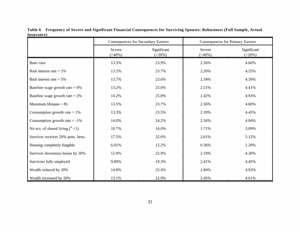
5. Robustness

In table 6, we examine the extent to which our estimated frequencies of significant and severe

uninsured vulnerabilities are sensitive to changes in key assumptions and parameters. To conserve space,

we focus on primary and secondary earners. For purposes of comparison, we reproduce our base-case

results in the first line of the table.

Changes in the real interest rate, baseline wage growth rate, and maximum lifespan are relatively

18For our base case, we assume that the inflation rate and real interest rate are both 3 percent.

20

inconsequential.18 In each case, this reflects the opposing effects of offsetting forces. With higher interest

rates, a given level of life insurance coverage generates higher real income. However, since survivors are

typically more dependent on long-duration life annuities than intact couples, the present discounted value of

their resources tends to decline by a larger proportion when the rate of return rises. For older workers, the

rate of wage growth is relatively unimportant because it affects comparatively few years of earnings.

Moreover, while a given rate of growth produces a larger absolute increase in earnings for primary earners,

secondary earners tend to be younger, and therefore benefit from higher growth over a longer time frame.

A reduction in maximum lifespan reduces the resources that a survivor needs to achieve a given living

standard, but increases the living standard that the intact couple can achieve from available resources.

The consumption growth rate refers to steepness of the sustainable living standard trajectory. For

our base-case, we compute the highest living standard that is sustainable throughout life in all contingencies;

this corresponds to a consumption growth rate of zero. For sufficiently patient (impatient) households, it may

be more natural to construct benchmarks based on a rising (falling) living standard trajectory. The

proportional effects of a change in the consumption growth rate on the resource needs of survivors and intact

couples are approximately equal. Our results are therefore robust with respect to changes in this parameter.

In contrast, our findings are sensitive to assumptions concerning household economies of scale,

pension survivor benefits, and housing. The frequencies of exposure to significant and severe financial

consequences are noticeably lower in the absence of household scale economies (an extreme and somewhat

implausible assumption), and higher when we reduce the rate of pension survivor benefits from 100 percent

to 50 percent.

As mentioned previously, our base case assumptions concerning housing are consistent with empirical

evidence indicating that older households avoid changing residences prior to death, and that they resist using

19Apparently, there is some sample selection: those who do not move are more likely to remain in thesample.

20In this exercise, we assume that the financing for the new house is the same as the continuation financingfor the old house. Consequently, upon a spouse’s death, the decline in home equity equals the reduction in thevalue of the home, and there is an offsetting increase in non-housing assets; mortgage payments are unchanged, butother housing expenses fall by 30 percent.

21

housing equity to finance ordinary living expenses. Analysis of the HRS panel corroborates the reluctance

to move among widows. By the second wave of the HRS (April 1994 through December 1994), 83.8 percent

of newly widowed women had not changed residence. Wave 3 (May 1996 through February 1997) contains

information on residences for 62.3 percent of these initial widows; 82.7 percent had not moved. Wave 4

(February 1998 through March 1999) contains information on 56.3 percent of the initial widows; 92.6 percent

had not moved.19

Since some widows do move, we examine sensitivity to two alternative assumptions. For the first,

we adopt the extreme position that housing consumption is completely and continuously flexible, and that

housing equity is a perfect substitute for other forms of wealth. For the second alternative, we adopt an

intermediate position: a survivor downsizes the couple’s primary residence by 30 percent, but thereafter avoids

using housing equity to finance ordinary living expenses.20 Though the first alternative dramatically reduces

the estimated frequencies of individuals at risk of severe or significant financial consequences, the effect of

the second alternative is small.

For our base case, we assume that survivors do not alter their labor force participation. Since non-

working wives approaching retirement age have limited employment options subsequent to their husbands’

deaths, this assumption is particularly appropriate for the HRS sample. Between the first two waves of the

HRS survey, only 2.9 percent of newly-widowed non-working women went back to work, compared with

4.0 percent of non-working non-widows; 6.7 percent of newly-widowed working women withdrew from the

labor force, compared with 9.3 percent of working non-widows. Thus, the net change in labor force

22

participation differed only slightly for these two groups. Only 5.6 percent of new widows said that they

increased their work hours subsequent to their husbands’ deaths; 4.2 percent said that they decreased their

hours, and 90.2 percent reported no change. On average, contemporaneously reported employment fell by

2.8 hours per week for widows, compared with 0.4 hours per week for non-widows. Results for subsequent

waves of the HRS are qualitatively similar.

To evaluate the sensitivity of our results with respect to possible changes in labor force participation,

we consider an extreme alternative assumption: all survivors, whether out of the labor force or employed part-

time, return to full-time employment. We impute full-time earnings based on regressions of earnings on

demographic characteristics, estimated separately for fully employed men and women. A survivor’s

contingent earnings are set equal to the maximum of imputed earnings and actual earnings. Due to familiar

sample selection problems, this procedure tends to overstate potential earnings for non-workers; it therefore

understates survivors’ financial vulnerabilities. As indicated in table 6, the estimated frequencies of financial

vulnerability are only moderately sensitive to this alternative assumption. This not particularly surprising.

Financial vulnerabilities are common even among dual-earner couples (recall table 5). Moreover, only 32

percent of the wives in our sample were not employed, and only 13 percent worked part-time.

In principle, shifts in non-labor income might also cushion the financial impact of a spouse’s death.

Our analysis makes no allowance for this possibility. Presumably, the most important source of potential

support is assistance from relatives. Between the first two waves of the HRS, only 6.2 percent of new

widows reported receiving any assistance of this type. Between the second and third waves, the figure was

7.5 percent; and between the third and fourth waves, it was only 2.5 percent. In addition, support may have

been modest and/or temporary in many of these cases. Consequently, there is little evidence that external

support payments are significant in practice.

If important economic variables are measured with error, our calculations may overstate the thickness

21The Life Insurance Marketing and Research Organization (LIMRA) has published statistics on ownershipof life insurance for 1984; see American Council of Life Insurance (1992). LIMRA classifies households by the ageof the household head. The percentages of households for which at least one member owned individual or grouplife insurance were as follows: 71 percent for age 65 and over, 91 percent for ages 55 through 64, and 89 percent forages 45-54. Average total coverage (inflated to 1992 dollars) among households with insurance was $17,959 for age65 and over, $64,681 for ages 55 through 64, and $110,998 for ages 45 through 54. The HRS sample cuts across thesethree age groups. At least one household member owned insurance for 84 percent of HRS households, and averagetotal coverage among households with insurance was $117,010.

22Wave 4 contains marital status information on 87.0 percent of women who were widowed between waves2 and 3.

23

of the upper and lower tails of the distribution of IMPACT, thereby exaggerating the frequencies of significant

and severe financial vulnerabilities. Measures of household assets tend to be particularly noisy. However,

as illustrated in the final two rows of table 6, our findings are not particularly sensitive to moderate changes

in the values of wealth (a 20 percent increase or decrease). Accurate measurement of life insurance

coverage is, of course, particularly critical for our analysis. Fortunately, the HRS data match up reasonably

well with other sources of information concerning this variable.21

As mentioned in section 2, we have ignored the possibility that remarriage might cushion the impact

of a spouse’s death. Since it is difficult to model the consequences of remarriage, we did not conduct

pertinent sensitivity analysis. However, given the age distribution of individuals in the HRS sample, the

assumption of no remarriage seems generally appropriate. Analysis of the HRS panel corroborates this

suspicion. By the second wave of the HRS, only 3.6 percent of newly widowed women had remarried.

Wave 3 contains information on marital status for 62.2 percent of these initial widows; 11.5 percent had

remarried. Wave 4 contains information on 56.7 percent of the initial widows; 10.6 percent had remarried.

Of those widowed between waves 2 and 3, less than one percent had remarried by wave 3, and only 4.3

percent had married by wave 4.22

Although the estimated fractions of individuals with significant and severe uninsured financial

vulnerabilities are sensitive to certain critical assumptions, it is important to emphasize that the poor correlation

24

between coverage and vulnerability is robust. From table 6, we see that the reduction in the estimated

incidence of vulnerability is largest when we assume either that there are no economies of shared living, that

housing expenditures are completely flexible, or that all survivors work full time. However, for all of these

alternative scenarios, simple probit and OLS regression (identical to those discussed in section 4) continue to

indicate that those with greater vulnerabilities (measured by IMPACT, ignoring insurance) are less likely to

have coverage, and have less coverage on average, than those with greater vulnerabilities.

6. Conclusions

Using data on older workers from the 1992 Health and Retirement Survey along with an elaborate

life-cycle planning model, we have quantified the extent to which the death of each individual would have

affected the financial status of his or her survivors, and we have measured the degree to which life insurance

holdings moderated these consequences. On average, life insurance was sufficient to avert significant

declines in survivors’ living standards. However, this average obscures a startling mismatch between

insurance holdings and underlying financial vulnerabilities. The impact of life insurance on the financial

security of at-risk individuals was surprisingly small. We have also identified household characteristics that

are correlated with uninsured financial vulnerabilities, as well as with the proclivity to address any given

degree of vulnerability by purchasing life insurance.

25

Table 1 Sample life insurance benchmarks

Insurance benchmarkfor husband

Insurance benchmarkfor wife

Base case 133,500 0

+ Age (58,54) 68,500 0

- Age (50,46) 192,000 0

+ Husband's earnings ($60K) 195,000 0

- Husband's earnings ($30K) 70,500 28,000

+ Wife's earnings ($30K) 111,500 69,000

- Wife's earnings ($0) 174,000 0

+ Child (age 16) 139,000 0

- Child 132,000 0

+ Earnings growth (2%) 143,500 0

- Earnings growth (0%) 125,000 0

+ Real interest rate (5%) 118,500 0

- Real interest rate (1%) 152,000 0

Assumptions for base case: age of husband: 54, age of wife: 50, husband’s employee earnings: $45,000,wife’s employee earnings: $25,000, husband’s retirement age: 64, wife’s retirement age: 63, number ofchildren: 1, age of child: 18, non-housing net wealth: $50,000, primary home value: $100,000, mortgagebalance: $20,000, earnings growth: 1%, real interest rate: 3%.

26

Table 2 Descriptive statistics

Table 2a: Household level variables

Mean Median

Non-housing net wealth 186,128 48,500

Primary home ownership 0.93 1

Primary home value 105,165 85,000

Household non-asset income 68,532 50,853

Number of children 0.23 0

Table 2b: Individual level variables

Husband Wife Primary earner Secondary earner

Mean Median Mean Median Mean Median Mean Median

Age 58 57 54 54 57 56 54 55

Non white 0.153 0 0.153 0 0.153 0 0.153 0

Gender 0 0 1 1 0.184 0 0.816 1

College degree 0.283 0 0.205 0 0.292 0 0.196 0

Pension coverage 0.471 0 0.363 0 0.526 1 0.308 0

Non-asset income 50,741 36,077 17,790 12,763 54,753 37,851 13,779 10,665

Actual life ins. 66,165 25,000 20,940 4,991 64,081 24,176 23,024 5,000

Benchmark lifeins.

62,098 0 17,126 0 72,103 1,688 7,121 0

) liv. std., ignoreins.

-6.62% 0.00% -17.6% 0.00% -3.93% 0.00% -20.3% -0.70%

) liv. std., actualif spouse dies

-1.81% 0.24% -4.49% 0.85% 0.70% 0.39% -7.00% 0.26%

Note: Actual and benchmark life insurance refer to insurance on the life of the individual listed at the topof the column. Changes in living standard () liv. std.) for the spouse listed at the top of each columndepend on insurance on the life of the other spouse.

27

Table 3 Distribution of Changes in Living Standard for Surviving Spouses

Panel A: Husbands and Wives

Surviving spouses are:

Wives Husbands

IMPACT Ignoring Insurance Actual Ignoring insurance Actual

<-40% 16.85% 11.03% 6.44% 5.06%

-40% to -20% 12.12% 9.37% 4.21% 2.98%

-20% to 0% 18.13% 15.95% 7.76% 6.96%

0% 52.91% 10.03% 81.59% 32.28%

0% to +20% - 43.59% - 49.93%

+20% to +40% - 6.25% - 1.85%

>+40% - 3.79% - 0.95%

Observations 2113 2113 2113 2113

Panel B: Primary and Secondary Earners

Surviving spouses are:

Secondary earners Primary earners

IMPACT Ignoring insurance Actual Ignoring insurance Actual

<-40% 20.26% 13.54% 3.03% 2.56%

-40% to -20% 13.16% 10.32% 3.17% 2.04%

-20% to 0% 17.13% 15.76% 8.76% 7.15%

0% 49.46% 9.56% 85.04% 32.75%

0% to +20% - 41.55% - 51.96%

+20% to +40% - 5.92% - 2.18%

>+40% - 3.36% - 1.37%

Observations 2113 2113 2113 2113

28

Table 4 Effect of Life Insurance on Changes in Living Standards for Surviving Spouses, byLevel of Vulnerability

Range forIMPACT,ignoring

insurance

Mean IMPACT Insurance Holdings

Survivingsouses are:

Ignoringinsurance

Actualinsurance

Percentuninsured

Meanbenchmark

Meanactual

Wives <-40% -72.6% -50.5% 27.5% 234,189 59,961

-40% to -20% -29.5% -15.6% 22.7% 119,120 59,494

0% to -20% -9.7% 4.1% 21.4% 45,293 63,319

0% 0.0% 9.8% 19.0% 0 70,643

Husbands <-40% -72.8% -62.6% 46.3% 171,016 22,568

-40% to -20% -28.1% -16.0% 33.7% 89,554 29,700

0% to -20% -9.7% -0.1% 26.8% 30,241 26,103

0% 0.0% 3.6% 39.6% 0 19,868

Secondary <-40% -72.7% -52.7% 30.1% 238,327 52,835

earners -40% to -20% -29.3% -14.9% 22.7% 122,388 59,065

0% to -20% -9.8% 4.7% 20.4% 45,101 62,279

0% 0.0% 9.7% 19.3% 0 70,645

Primary <-40% -72.5% -61.6% 50.0% 72,271 28,156

earners -40% to -20% -28.5% -19.2% 37.3% 66,287 21,698

0% to -20% -9.4% -0.8% 28.1% 32,324 32,363

0% 0.0% 3.8% 38.5% 0 21,929

29

Table 5 Frequency of Severe and Significant Financial Consequences for Surviving Spouses: Selected Population Subgroups

Consequences for Secondary Earners Consequences for Primary Earners

Severe(>40%)

Significant(>20%)

Severe(>40%)

Significant(>20%)

Freq.Actual

Freq. Ins=0

Frac.Addr.

Freq.Actual

FreqIns=0

Frac.Addr.

Freq.Actual

Freq Ins=0

Frac.Addr.

Freq.Actual

FreqIns=0

Frac.Addr.

Full sample 13.5% 20.3% 0.335 23.9% 33.4% 0.284 2.56% 3.03% 0.155 4.60% 6.20% 0.258

HH earnings < $45K20.5%

27.0% 0.241 31.0% 40.0% 0.225 5.37% 5.83% 0.080 7.93% 9.57% 0.171

HH earnings $45-$100K 7.62% 15.1% 0.495 17.3% 28.4% 0.391 0.68% 1.25% 0.456 2.51% 4.15% 0.395

HH earnings > $100K 14.2% 18.4% 0.228 27.1% 31.7% 0.145 0.46% 0.46% 0.000 1.38% 2.75% 0.498

Dual earners 12.1% 18.5% 0.346 22.8% 32.4% 0.296 3.11% 3.64% 0.146 5.64% 7.52% 0.250

Single earners 19.6% 27.6% 0.290 28.4% 37.7% 0.247 0.24% 0.49% 0.510 0.24% 0.73% 0.671

Earnings diff. 1-1 to 2-1 8.52% 12.5% 0.318 17.5% 25.0% 0.300 5.49% 6.32% 0.131 10.6% 13.9% 0.237

Earnings diff. over 4-1 18.6% 27.7% 0.329 29.6% 40.4% 0.267 0.32% 0.54% 0.407 0.32% 0.65% 0.508

Age of survivor: 40-49 15.8% 27.3% 0.421 29.8% 43.8% 0.320 6.60% 7.55% 0.126 11.3% 11.3% 0.000

Age of survivor: 50-59 14.2% 20.9% 0.321 25.2% 35.1% 0.282 2.53% 2.97% 0.148 4.49% 6.23% 0.279

Age of survivor: 60-69 8.90% 12.6% 0.294 14.1% 19.9% 0.291 1.35% 1.86% 0.274 3.21% 4.90% 0.345

No children 12.3% 18.8% 0.346 22.7% 31.6% 0.282 2.27% 2.78% 0.183 4.20% 5.79% 0.275

One or more child 19.8% 27.5% 0.280 29.8% 42.7% 0.302 4.01% 4.30% 0.070 6.59% 8.31% 0.207

Whites 11.2% 17.9% 0.374 21.0% 31.0% 0.323 1.90% 2.23% 0.148 3.69% 5.08% 0.274

Non-whites 26.4% 33.2% 0.205 39.8% 46.9% 0.151 6.23% 7.48% 0.167 9.66% 12.5% 0.227

30

31

Table 6 Frequency of Severe and Significant Financial Consequences for Surviving Spouses: Robustness (Full Sample, ActualInsurance)

Consequences for Secondary Earners Consequences for Primary Earners

Severe(>40%)

Significant(>20%)

Severe(>40%)

Significant(>20%)

Base case 13.5% 23.9% 2.56% 4.60%

Real interest rate = 1% 13.2% 23.7% 2.20% 4.55%

Real interest rate = 5% 13.7% 23.6% 2.34% 4.39%

Baseline wage growth rate = 0% 13.2% 23.0% 2.51% 4.41%

Baseline wage growth rate = 2% 14.2% 25.0% 2.42% 4.93%

Maximum lifespan = 85 13.5% 23.7% 2.56% 4.60%

Consumption growth rate = 1% 13.3% 23.5% 2.39% 4.45%

Consumption growth rate = -1% 14.0% 24.2% 2.56% 4.84%

No ecs. of shared living ("=1) 10.7% 16.0% 1.71% 3.09%

Survivor receives 50% pens. bens. 17.5% 32.0% 2.61% 5.12%

Housing completely fungible 6.01% 12.2% 0.36% 1.20%

Survivor downsizes house by 30% 12.9% 22.9% 2.18% 4.30%

Survivors fully employed 9.89% 19.3% 2.41% 4.45%

Wealth reduced by 20% 14.8% 25.4% 2.84% 4.93%

Wealth increased by 20% 13.1% 22.9% 2.45% 4.61%

32

References

American Council of Life Insurance, 1992 Life Insurance Fact Book , American Council of Life Insurance:Washington, DC, 1992.

Auerbach, Alan J., and Laurence J. Kotlikoff, “Life Insurance of the Elderly: Its Adequacy andDeterminants,” in G. Burtless (ed.), Work, Health, and Income Among the Elderly, The Brookings Institution,Washington D.C., 1987.

Auerbach, Alan J., and Laurence J. Kotlikoff, “Life Insurance Inadequacy - Evidence from a Sample ofOlder Widows,” National Bureau of Economic Research Working Paper No. 3765, 1991a.

Auerbach, Alan J., and Laurence J. Kotlikoff, “The Adequacy of Life Insurance Purchases,” Journal ofFinancial Intermediation, 1(3), June 1991b, 215-241.

Bernheim, B. Douglas, “The Economic Effects of Social Security: Towards a Reconciliation of Theory andMeasurement,” Journal of Public Economics 33 (3), August 1987, 273-304.

Bernheim, B. Douglas, Lorenzo Forni, Jagadeesh Gokhale, and Laurence J. Kotlikoff, “The Adequacy of LifeInsurance: Evidence from the Health and Retirement Survey,” NBER working paper no. 7372, October 1999.

Caplin, Andrew, “The Reverse Mortgage Market: Problems and Prospects,” in Zvi Bodie, Brett Hammond,Olivia Mitchell, and Steven Zeldes (eds.), Innovations in Managing the Financial Risks of Retirement,Pension Reserach Council, the Wharton School, University of Pennsylvania, forthcoming, 2000.

Gokhale, Jagadeesh, Laurence J. Kotlikoff, and Mark Warshawsky, “Financial Planning -- The Economic vs.the Conventional Approach,” mimeo, NBER working paper, 1999.

Holden, K.C., R.V. Burkhauser, and D.A. Myers, “Pensioners’ Annuity Choice: Is the Well-Being of theirWidows Considered?” University of Wisconsin Institute for Research on Poverty Discussion Paper 802-86,1986.

Hurd, Michael D. and David A. Wise, “The Wealth and Poverty of Widows: Assets Before and After theHusband’s Death,” in D. Wise (ed.), The Economics of Aging, Chicago and London: University of ChicagoPress, 1989, 177-99.

Kotlikoff, Laurence J. and Avia Spivak, “The Family as an Incomplete Annuities Market,” Journal of PoliticalEconomy, 89 (2), April 1981, 372-91.

Kotlikoff, Laurence J., What Determines Savings?, Cambridge, MA.: MIT Press, 1989

Lundberg, Shelly, “Family Bargaining and Retirement Behavior,” in Henry Aaron (ed.), Behavioral Economicsand Retirement Policy, Brookings Institution, 1999 (forthcoming).

Mitchell, Olivia S. and James F., Moore, “Retirement Wealth Accumulation and Decumulation: New

33

Developments and Outstanding Opportunities,” NBER working paper, no. 6178, 1997a.

Mitchell, Olivia S. and James F., Moore, “Projected Retirement Wealth and Savings Adequacy in the Healthand Retirement Study,” NBER working paper, no. 6240, 1997b.

Mitchell, Olivia S., James M. Poterba, Mark J. Warshawsky, and Jeffrey R. Brown, “New Evidence on theMoney’s Worth of Individual Annuities,” American Economic Review 89(5), December 1999, 1299-1318.

Nelson, Julie A., “Methods of Estimating Household Equivalence Scales: An Empirical Investigation,” Reviewof Income and Wealth, 38 (3), September 1992.

Ringen, S. “Households, Standard of Living, and Inequality,” Review of Income and Wealth, 37, 1991, 1-13.

Venti, Steve, and David Wise, “Patterns of Housing Equity Use Among the Elderly,” in Zvi Bodie, BrettHammond, Olivia Mitchell, and Steven Zeldes (eds.), Innovations in Managing the Financial Risks ofRetirement, Pension Reserach Council, the Wharton School, University of Pennsylvania, forthcoming,2000.

Williams, Roberton, David Weiner, and Frank Sammartino, “Equivalence Scales, the Income Distribution, andFederal Taxes,” Technical Paper Series 1999-2, Congressional Budget Office, October 1998.

Yaari, Menachem, “Uncertain Lifetime, Life Insurance, and the Theory of the Consumer,” Review ofEconomic Studies, 32, April 1965, 137-50.

23In this analysis, we restrict attention to policies that name the spouse or children living in the householdas beneficiaries. Roughly 5 percent of individuals hold a life insurance policy that names some other party or entity(such as a trust) as beneficiary.

24The HRS reports only the sum of child support and spousal support. However, we confine our attentionto couples, 98 percent of which are married. Since spousal support generally ends upon remarriage (and alsodeclines somewhat on average when individuals become unmarried partners), we can safely assume that the entirereported amount is child support.

34

Appendix

Data Imputation

Life Insurance. The HRS collects information about term and whole life insurance policies, but not the termcomponent of whole life policies. We impute the term component using a regression explaining the ratio ofcash value to face value as a function of the age of each spouse, the face value of the policy, family income,family size, and financial assets. We estimate this regression using data from the 1995 Survey of ConsumerFinances (SCF).23

Non-Asset Income. Our calculations require data on each spouse’s past and future covered earnings as wellas future total (covered and uncovered) earnings. We obtain past covered earnings from the HRS restricteddata file. We impute future covered and total earnings as follows. First, we adjust actual earnings in thecurrent year (1991) to remove the effects of temporary fluctuations. Specifically, we assume that actualearnings for 1991 equaled the maximum of 1991 reported earnings and 1991 covered earnings. We thendefine adjusted covered earnings in year t # 1991 as covered earnings in year t adjusted for inflation to 1991dollars, multiplied by (1 + assumed earnings growth rate) (1991-t). Next, we define normal adjusted coveredearnings as a five year average (1987-1991) of adjusted covered earnings. We then set normal earningsequal to 1991 earnings times the ratio of normal adjusted covered earnings to 1991 covered earnings. Tocompute future earnings, we let normal earnings grow at the assumed real earnings growth rate. We obtainfuture covered earnings directly from imputed future earnings based on applicable statutes.

The HRS provides information on other kinds of non-asset income. We treat some of these income sources,such as Veteran’s Benefits, SSI, disability income, welfare, child support, and regular help from friends orrelatives, as non-taxable. Except for Social Security disability income and child support, we assume theseincome streams continue, with full adjustments for inflation, until the respondent’s death. Social Securitydisability income is assumed to end at age 62, when the recipient becomes eligible for Social Securityretirement benefits. We divide child support received by the number of children to obtain child support perchild and assume it is received until the child in question reaches 18.24 We treat other kinds of specialreceipts, such as income from trust funds and royalties, as taxable. We assume they will be received for tenyears beyond the survey date, and that the payments will be constant in nominal terms. Relatively fewrespondents receive these kinds of income flows, and the amounts are generally small relative to averageearnings. We assume that HRS respondents retire at their stated intended ages of retirement or age 70,whichever is smaller. For those who fail to say when they will retire, we use age 65.

Pension Plans, Retirement Accounts, and Social Security. The HRS provides information on nominal benefitscurrently received from defined benefit pension plans as well as expected nominal benefits for future pension

25The ownership of these balances influences the timing of withdraws. This, in turns, affects tax liabilities. The timing of withdrawals also may determine whether the couple is liquidity constrained as it approachesretirement.

35

recipients. It also indicates whether these benefits are indexed for inflation. We assume that a survivingspouse would receive 100 percent of the monthly benefit or lump-sum distribution. We further assume thatemployer-sponsored defined contribution plans and all private retirement accounts (IRAs and Keoghs) providefor tax-deductible contributions and tax-deferred accumulation. Contributions in all future years up to age59 are set equal, in real terms, to contributions in the survey year. The HRS contains information on 401(k)accounts for individual spouses, but IRA and Keogh account balances are reported only at the householdlevel. We impute each spouse’s IRA and Keogh account balances and contribution amounts based on theirshare of 1991 household labor earnings.25

We code an individual as having a pension or retirement account of a particular type if and only if theindividual affirmatively indicates that he or she had such a pension or retirement account. If the individualprovides insufficient information to ascertain whether he or she had a pension or retirement account (forexample, if the response was “don’t know”), we assume that no such account exists.

If an individual is already receiving Social Security benefits, we assume that benefits have already started.Otherwise, we impute the initial age of benefit receipt as follows. If the individual is still working, we assumethat benefits will start at his or her projected retirement age (but not earlier than age 62). If the individual isretired, we assume that benefits will start at age 62 for those currently under 62, and at the current age forthose over 62. In all cases, the initial age of benefit receipt is between 62 and 70. For respondents currentlyreceiving social security disability benefits, we assume that they switch to retirement benefits at age 62.

Our calculations also require information on the age at which individuals begin to receive private pensionbenefits. If the individual is already receiving benefits, we assume that benefits have already started. If theindividual is not receiving benefits, but indicates the age at which he or she expects benefits to begin, we usethat age. Otherwise, we impute the initial age of pension benefit receipt in exactly the same manner as forSocial Security retirement benefits, based on work status, current age, and projected retirement age. In allcases, we truncate the benefit inception date at 70.

Individuals with previous marriages lasting more than ten years and ending in divorce or separation (roughly20 percent of the total HRS sample), and individuals with previous marriages lasting more than nine monthsand ending in the spouse’s death (roughly 8 percent of the total HRS sample) are eligible to receive SocialSecurity benefits based on the earnings history of their prior spouse. This presents us with a problem, sincewe do not have access to covered earnings histories for prior spouses. We assume that all such individualsreceive benefits based on either their own earnings history or that of their current spouse.

Housing. Our calculations require information on a variety of specific housing expenditures, includingmortgages, home insurance premiums, property taxes, and other recurring expenses. The HRS containsdetailed information on recurring expenses such as association fees and site rental charges for householdsliving in mobile homes. While it does not contain information on home insurance premiums, it does includethe face amount of insurance. We imputed annual home insurance premiums by assuming a rate of $0.0025

26Ten respondents did not report month of birth; we assume they were born in June.

34

for each dollar of insurance coverage. Information on property taxes is usually available. When it is not, weimpute it using the home value and applying the average ratio of property taxes to home value obtained fromthe rest of the sample.

In some instances, mortgage payments reported in the sample include property taxes and home insurancepremiums; in such cases, respondents were not asked separately about their taxes and premiums. We imputeproperty taxes from home value by applying the average ratio of property tax to house value for our entiresample. Similarly, we impute insurance premiums by applying the average ratio of (imputed) insurancepremium to house value for our entire sample. We assume that the mortgage payment accounts for anyresidual.

Unfortunately, the HRS does not report the number of years left on each mortgage. We assume that eachhousehold took out a 30 year mortgage in the year it purchased its home (which is reported in the HRS), andthat it has never refinanced; this allows us to compute the number of years remaining on the mortgage. Incases where the respondent did not report a mortgage payment, we impute one based on the reportedbalance, the imputed number of years left in the loan, and a representative mortgage interest rate for 1991.

In some instances, rental payments reported in the sample include heat and electricity expenses; in suchcases, respondents were not asked separately about these utility payments. We apportion the reportednumber into separate components by assuming that the ratio of rent to utilities is the same for theserespondents as the average ratio computed from the rest of the sample. The HRS does not include anyinformation concerning property taxes paid on second homes. We calculate these from second home valuesbased on the assumption that the ratio of property taxes to value is the same as the average for primaryhomes (0.0018 monthly). Finally, we set monthly rental payments equal to zero for the few respondents whoreport that they live in a house or apartment that they neither rent nor own.

Other Variables. For confidentiality reasons, the HRS does not report the respondent’s date of birth or stateof residency. We assume that each respondent was born on the fifteenth of his or her birth month.26 For thepurposes of computing state taxes, we use Massachusetts law. We set the maximum age of life to 95 forall individuals. We assume that funeral expenses and associated legal fees for deceased spouses will be equal(in real terms) to the sample median for those who died in 1991 ($5,000, based on 90 observations). Asidefrom funerals, we do not impute any other special expenditures. We set intended bequests equal to zero. Asa measure of a household’s net worth, we use total non-housing assets minus total non-housing liabilities.Total non-housing assets include checking and saving accounts, money market funds, CDs, government savingbonds, T-bills, stocks, mutual funds, investment trusts, business equity, bonds, bond funds, real estate otherthan primary and vacation homes, the cash value of life insurance policies, and some miscellaneous items.Total non-housing liabilities include personal loans, student loans, credit card balances, car loans, installmentloans, and other non housing debt. Housing debt (mortgages and equity lines of credit) are consideredseparately (see above). We assume that, apart from mortgages and other outstanding housing debt,households cannot borrow against future income. For our base case, we use a 3 percent rate of inflation anda 3 percent real pre-tax rate of return.

35