the microfluidics module user’s guide

Microfluidics ModuleUser’s Guide

C o n t a c t I n f o r m a t i o n

Visit the Contact COMSOL page at www.comsol.com/contact to submit general inquiries, contact Technical Support, or search for an address and phone number. You can also visit the Worldwide Sales Offices page at www.comsol.com/contact/offices for address and contact information.

If you need to contact Support, an online request form is located at the COMSOL Access page at www.comsol.com/support/case. Other useful links include:

• Support Center: www.comsol.com/support

• Product Download: www.comsol.com/product-download

• Product Updates: www.comsol.com/support/updates

• COMSOL Blog: www.comsol.com/blogs

• Discussion Forum: www.comsol.com/community

• Events: www.comsol.com/events

• COMSOL Video Gallery: www.comsol.com/video

• Support Knowledge Base: www.comsol.com/support/knowledgebase

Part number: CM021901

M i c r o f l u i d i c s M o d u l e U s e r ’ s G u i d e © 1998–2018 COMSOL

Protected by patents listed on www.comsol.com/patents, and U.S. Patents 7,519,518; 7,596,474; 7,623,991; 8,457,932; 8,954,302; 9,098,106; 9,146,652; 9,323,503; 9,372,673; and 9,454,625. Patents pending.

This Documentation and the Programs described herein are furnished under the COMSOL Software License Agreement (www.comsol.com/comsol-license-agreement) and may be used or copied only under the terms of the license agreement.

COMSOL, the COMSOL logo, COMSOL Multiphysics, COMSOL Desktop, COMSOL Server, and LiveLink are either registered trademarks or trademarks of COMSOL AB. All other trademarks are the property of their respective owners, and COMSOL AB and its subsidiaries and products are not affiliated with, endorsed by, sponsored by, or supported by those trademark owners. For a list of such trademark owners, see www.comsol.com/trademarks.

Version: COMSOL 5.4

www.comsol.com/patents/

http://www.comsol.com/comsol-license-agreement/

http://www.comsol.com/contact/

http://www.comsol.com/contact/offices/

http://www.comsol.com/support/case/

http://www.comsol.com/support/

http://www.comsol.com/product-download/

http://www.comsol.com/support/updates/

http://www.comsol.com/trademarks/

http://www.comsol.com/blogs/

http://www.comsol.com/community/

http://www.comsol.com/events/

http://www.comsol.com/video/

http://www.comsol.com/support/knowledgebase/

C o n t e n t s

C h a p t e r 1 : I n t r o d u c t i o n

About the Microfluidics Module 14

About Microfluidics . . . . . . . . . . . . . . . . . . . . . . 14

About the Microfluidics Module . . . . . . . . . . . . . . . . . 15

The Microfluidics Module Physics Interface Guide . . . . . . . . . . 15

Coupling to Other Physics Interfaces . . . . . . . . . . . . . . . 18

The Microfluidics Module Study Capabilities by Physics Interface . . . . . 19

Common Physics Interface and Feature Settings and Nodes . . . . . . 20

The Liquids and Gases Materials Database . . . . . . . . . . . . . 21

Where Do I Access the Documentation and Application Libraries? . . . . 21

Overview of the User’s Guide 25

C h a p t e r 2 : M i c r o f l u i d i c M o d e l i n g

Physics and Scaling in Microfluidics 28

Dimensionless Numbers in Microfluidics 31

Dimensionless Numbers Important for Solver Stability . . . . . . . . 31

Other Dimensionless Numbers . . . . . . . . . . . . . . . . . 33

Modeling Microfluidic Fluid Flows 36

Selecting the Right Physics Interface. . . . . . . . . . . . . . . . 36

Single-Phase Flow . . . . . . . . . . . . . . . . . . . . . . 37

Multiphase Flow . . . . . . . . . . . . . . . . . . . . . . . 39

Porous Media Flow . . . . . . . . . . . . . . . . . . . . . . 40

The Relationship Between the Physics Interfaces . . . . . . . . . . . 42

Modeling Coupled Phenomena in Microfluidics 44

Chemical Transport and Reactions . . . . . . . . . . . . . . . . 44

Electrohydrodynamics . . . . . . . . . . . . . . . . . . . . . 46

C O N T E N T S | 3

4 | C O N T E N T S

Heat Transfer . . . . . . . . . . . . . . . . . . . . . . . . 53

Coupling to Other Physics Interfaces . . . . . . . . . . . . . . . 55

Modeling Rarefied Gas Flows 56

The Flow Regimes . . . . . . . . . . . . . . . . . . . . . . 56

Slip Flow . . . . . . . . . . . . . . . . . . . . . . . . . . 57

References for the Theory of Microfluidics . . . . . . . . . . . . . 58

C h a p t e r 3 : S i n g l e - P h a s e F l o w I n t e r f a c e s

The Laminar Flow and Creeping Flow Interfaces 60

The Creeping Flow Interface . . . . . . . . . . . . . . . . . . 60

The Laminar Flow Interface . . . . . . . . . . . . . . . . . . . 61

Fluid Properties . . . . . . . . . . . . . . . . . . . . . . . 66

Volume Force . . . . . . . . . . . . . . . . . . . . . . . . 69

Initial Values . . . . . . . . . . . . . . . . . . . . . . . . 69

Wall . . . . . . . . . . . . . . . . . . . . . . . . . . . 70

Inlet . . . . . . . . . . . . . . . . . . . . . . . . . . . . 72

Outlet . . . . . . . . . . . . . . . . . . . . . . . . . . . 75

Symmetry . . . . . . . . . . . . . . . . . . . . . . . . . 77

Open Boundary . . . . . . . . . . . . . . . . . . . . . . . 78

Boundary Stress . . . . . . . . . . . . . . . . . . . . . . . 78

Periodic Flow Condition . . . . . . . . . . . . . . . . . . . . 80

Flow Continuity . . . . . . . . . . . . . . . . . . . . . . . 81

Pressure Point Constraint . . . . . . . . . . . . . . . . . . . 81

Point Mass Source . . . . . . . . . . . . . . . . . . . . . . 81

Line Mass Source . . . . . . . . . . . . . . . . . . . . . . . 82

Gravity . . . . . . . . . . . . . . . . . . . . . . . . . . 83

Theory for the Single-Phase Flow Interfaces 85

General Single-Phase Flow Theory . . . . . . . . . . . . . . . . 86

Compressible Flow . . . . . . . . . . . . . . . . . . . . . . 88

Weakly Compressible Flow . . . . . . . . . . . . . . . . . . . 88

The Mach Number Limit . . . . . . . . . . . . . . . . . . . . 88

Incompressible Flow . . . . . . . . . . . . . . . . . . . . . 89

The Reynolds Number. . . . . . . . . . . . . . . . . . . . . 90

Non-Newtonian Flow . . . . . . . . . . . . . . . . . . . . . 91

Theory for the Wall Boundary Condition . . . . . . . . . . . . . 93

Prescribing Inlet and Outlet Conditions . . . . . . . . . . . . . . 97

Mass Flow . . . . . . . . . . . . . . . . . . . . . . . . . 98

Fully Developed Flow (Inlet) . . . . . . . . . . . . . . . . . 100

Fully Developed Flow (Outlet). . . . . . . . . . . . . . . . . 101

No Viscous Stress . . . . . . . . . . . . . . . . . . . . . 102

Normal Stress Boundary Condition . . . . . . . . . . . . . . . 103

Pressure Boundary Condition . . . . . . . . . . . . . . . . . 103

Mass Sources for Fluid Flow . . . . . . . . . . . . . . . . . 105

Numerical Stability — Stabilization Techniques for Fluid Flow . . . . . 107

Solvers for Laminar Flow . . . . . . . . . . . . . . . . . . . 109

Pseudo Time Stepping for Laminar Flow Models . . . . . . . . . . 111

Discontinuous Galerkin Formulation . . . . . . . . . . . . . . 113

Particle Tracing in Fluid Flow . . . . . . . . . . . . . . . . . 113

References for the Single-Phase Flow, Laminar Flow Interfaces . . . . 114

C h a p t e r 4 : M u l t i p h a s e F l o w , T w o - P h a s e F l o w

I n t e r f a c e s

The Laminar Two-Phase Flow, Level Set and Laminar

Two-Phase Flow, Phase Field Interfaces 118

The Laminar Two-Phase Flow, Level Set Interface . . . . . . . . . 118

T he Two-Phase Flow, Level Set Coupling Feature . . . . . . . . . 119

The Wetted Wall Coupling Feature. . . . . . . . . . . . . . . 122

The Laminar Two-Phase Flow, Phase Field Interface . . . . . . . . 124

The Two-Phase Flow, Phase Field Coupling Feature. . . . . . . . . 124

Domain, Boundary, Point, and Pair Nodes for the Laminar Flow,

Two-Phase, Level Set and Phase Field Interfaces . . . . . . . . . 127

The Laminar Three-Phase Flow, Phase Field Interface 129

The Laminar Three-Phase Flow, Phase Field Interface . . . . . . . . 129

The Three-Phase Flow, Phase Field Coupling Feature . . . . . . . . 130

Domain, Boundary, Point, and Pair Nodes for the Laminar

Three-Phase Flow, Phase Field Interface . . . . . . . . . . . . 132

C O N T E N T S | 5

6 | C O N T E N T S

The Laminar Two-Phase Flow, Moving Mesh Interface 134

Select Laminar Flow Properties . . . . . . . . . . . . . . . . 135

Deforming Domain . . . . . . . . . . . . . . . . . . . . . 135

Fluid-Fluid Interface . . . . . . . . . . . . . . . . . . . . . 136

External Fluid Interface . . . . . . . . . . . . . . . . . . . 137

Wall-Fluid Interface . . . . . . . . . . . . . . . . . . . . . 139

Theory for the Level Set and Phase Field Interfaces 141

Level Set and Phase Field Equations . . . . . . . . . . . . . . . 141

Conservative and Nonconservative Formulations . . . . . . . . . 144

Phase Initialization . . . . . . . . . . . . . . . . . . . . . 145

Numerical Stabilization . . . . . . . . . . . . . . . . . . . 146

References for the Level Set and Phase Field Interfaces . . . . . . . 146

Theory for the Three-Phase Flow, Phase Field Interface 148

Governing Equations of the Three-Phase Flow, Phase Field Interface . . 148

Reference for the Three-Phase Flow, Phase Field Interface . . . . . . 151

Theory for the Two-Phase Flow, Moving Mesh Interface 152

Domain Level Fluid Flow . . . . . . . . . . . . . . . . . . . 152

About the Moving Mesh . . . . . . . . . . . . . . . . . . . 153

About the Fluid Interface Boundary Conditions . . . . . . . . . . 154

Wall-Fluid Interface Boundary Conditions . . . . . . . . . . . . 158

References for the Two-Phase Flow, Moving Mesh Interface . . . . . 159

C h a p t e r 5 : M a t h e m a t i c s , M o v i n g I n t e r f a c e s

The Level Set Interface 162

Domain, Boundary, and Pair Nodes for the Level Set Interface . . . . 163

Level Set Model . . . . . . . . . . . . . . . . . . . . . . 164

Initial Values . . . . . . . . . . . . . . . . . . . . . . . 164

Inlet . . . . . . . . . . . . . . . . . . . . . . . . . . . 165

Initial Interface . . . . . . . . . . . . . . . . . . . . . . . 166

No Flow . . . . . . . . . . . . . . . . . . . . . . . . . 166

Thin Barrier. . . . . . . . . . . . . . . . . . . . . . . . 166

The Phase Field Interface 167

Domain, Boundary, and Pair Nodes for the Phase Field Interface . . . . 168

Phase Field Model . . . . . . . . . . . . . . . . . . . . . 169

Initial Values . . . . . . . . . . . . . . . . . . . . . . . 170

Inlet . . . . . . . . . . . . . . . . . . . . . . . . . . . 171

Initial Interface . . . . . . . . . . . . . . . . . . . . . . . 171

Wetted Wall . . . . . . . . . . . . . . . . . . . . . . . 171

Interior Wetted Wall . . . . . . . . . . . . . . . . . . . . 172

The Ternary Phase Field Interface 173

Domain, Boundary, and Pair Nodes for the Ternary Phase Field

Interface. . . . . . . . . . . . . . . . . . . . . . . . 174

Mixture Properties . . . . . . . . . . . . . . . . . . . . . 174

Initial Values . . . . . . . . . . . . . . . . . . . . . . . 176

Inlet . . . . . . . . . . . . . . . . . . . . . . . . . . . 176

Outlet . . . . . . . . . . . . . . . . . . . . . . . . . . 176

Symmetry . . . . . . . . . . . . . . . . . . . . . . . . 177

Wetted Wall . . . . . . . . . . . . . . . . . . . . . . . 177

Theory for the Level Set Interface 179

The Level Set Method . . . . . . . . . . . . . . . . . . . . 179

Conservative and Nonconservative Form . . . . . . . . . . . . 181

Initializing the Level Set Function . . . . . . . . . . . . . . . . 182

Variables For Geometric Properties of the Interface . . . . . . . . 182

Reference for the Level Set Interface . . . . . . . . . . . . . . 183

Theory for the Phase Field Interface 184

About the Phase Field Method. . . . . . . . . . . . . . . . . 184

The Equations for the Phase Field Method . . . . . . . . . . . . 184

Conservative and Nonconservative Forms . . . . . . . . . . . . 186

Additional Sources of Free Energy . . . . . . . . . . . . . . . 187

Initializing the Phase Field Function . . . . . . . . . . . . . . . 187

Variables and Expressions . . . . . . . . . . . . . . . . . . 188

Reference for the Phase Field Interface . . . . . . . . . . . . . 188

Theory for the Ternary Phase Field Interface 189

About the Phase Field Method. . . . . . . . . . . . . . . . . 189

The Equations of the Ternary Phase Field Method . . . . . . . . . 189

C O N T E N T S | 7

8 | C O N T E N T S

Reference for the Ternary Phase Field Interface . . . . . . . . . . 191

C h a p t e r 6 : P o r o u s M e d i a F l o w I n t e r f a c e s

The Darcy’s Law Interface 194

Domain, Boundary, Edge, Point, and Pair Nodes for the Darcy’s

Law Interface . . . . . . . . . . . . . . . . . . . . . . 195

Fluid and Matrix Properties . . . . . . . . . . . . . . . . . . 197

Mass Source . . . . . . . . . . . . . . . . . . . . . . . 198

Initial Values . . . . . . . . . . . . . . . . . . . . . . . 198

Pressure . . . . . . . . . . . . . . . . . . . . . . . . . 198

Mass Flux. . . . . . . . . . . . . . . . . . . . . . . . . 199

Inlet . . . . . . . . . . . . . . . . . . . . . . . . . . . 199

Symmetry . . . . . . . . . . . . . . . . . . . . . . . . 200

No Flow . . . . . . . . . . . . . . . . . . . . . . . . . 200

Flux Discontinuity . . . . . . . . . . . . . . . . . . . . . 200

Outlet . . . . . . . . . . . . . . . . . . . . . . . . . . 201

Cross Section . . . . . . . . . . . . . . . . . . . . . . . 201

Thickness. . . . . . . . . . . . . . . . . . . . . . . . . 202

The Brinkman Equations Interface 203

Domain, Boundary, Point, and Pair Nodes for the Brinkman

Equations Interface . . . . . . . . . . . . . . . . . . . . 205


Forchheimer Drag . . . . . . . . . . . . . . . . . . . . . 207

Mass Source . . . . . . . . . . . . . . . . . . . . . . . 207

Volume Force . . . . . . . . . . . . . . . . . . . . . . . 208

Initial Values . . . . . . . . . . . . . . . . . . . . . . . 208

Fluid Properties . . . . . . . . . . . . . . . . . . . . . . 208

The Free and Porous Media Flow Interface 210

Domain, Boundary, Point, and Pair Nodes for the Free and Porous

Media Flow Interface . . . . . . . . . . . . . . . . . . . 211

Fluid Properties . . . . . . . . . . . . . . . . . . . . . . 212


Volume Force . . . . . . . . . . . . . . . . . . . . . . . 214

Forchheimer Drag . . . . . . . . . . . . . . . . . . . . . 214

Initial Values . . . . . . . . . . . . . . . . . . . . . . . 214

Microfluidic Wall Conditions . . . . . . . . . . . . . . . . . 214

Wall . . . . . . . . . . . . . . . . . . . . . . . . . . 215

Theory for the Darcy’s Law Interface 217

Darcy’s Law — Equation Formulation . . . . . . . . . . . . . . 217

Theory for the Brinkman Equations Interface 219

About the Brinkman Equations . . . . . . . . . . . . . . . . 219

Brinkman Equations Theory. . . . . . . . . . . . . . . . . . 220

References for the Brinkman Equations Interface. . . . . . . . . . 221

Theory for the Free and Porous Media Flow Interface 222

Reference for the Free and Porous Media Flow Interface. . . . . . . 222

C h a p t e r 7 : R a r e f i e d F l o w I n t e r f a c e

The Slip Flow Interface 224

Domain, Boundary, Edge, Point, and Pair Nodes for the Slip Flow

Interface. . . . . . . . . . . . . . . . . . . . . . . . 226

Fluid . . . . . . . . . . . . . . . . . . . . . . . . . . 227

External Slip Wall . . . . . . . . . . . . . . . . . . . . . 228

Initial Values . . . . . . . . . . . . . . . . . . . . . . . 229

Slip Wall . . . . . . . . . . . . . . . . . . . . . . . . . 229

Periodic Condition . . . . . . . . . . . . . . . . . . . . . 230

Symmetry . . . . . . . . . . . . . . . . . . . . . . . . 230

Continuity . . . . . . . . . . . . . . . . . . . . . . . . 230

Theory for the Slip Flow Interface 231

Slip Flow Boundary Conditions . . . . . . . . . . . . . . . . 231

References for the Slip Flow Interface . . . . . . . . . . . . . . 233

C O N T E N T S | 9

10 | C O N T E N T S

C h a p t e r 8 : C h e m i c a l S p e c i e s T r a n s p o r t I n t e r f a c e s

The Transport of Diluted Species Interface 236

The Transport of Diluted Species in Porous Media Interface . . . . . 240

Domain, Boundary, and Pair Nodes for the Transport of Diluted

Species Interface. . . . . . . . . . . . . . . . . . . . . 241

Transport Properties . . . . . . . . . . . . . . . . . . . . 243

Turbulent Mixing . . . . . . . . . . . . . . . . . . . . . . 245

Initial Values . . . . . . . . . . . . . . . . . . . . . . . 246

Mass-Based Concentrations . . . . . . . . . . . . . . . . . . 246

Reactions. . . . . . . . . . . . . . . . . . . . . . . . . 246

No Flux . . . . . . . . . . . . . . . . . . . . . . . . . 248

Inflow . . . . . . . . . . . . . . . . . . . . . . . . . . 248

Outflow . . . . . . . . . . . . . . . . . . . . . . . . . 249

Concentration . . . . . . . . . . . . . . . . . . . . . . . 249

Flux . . . . . . . . . . . . . . . . . . . . . . . . . . . 249

Symmetry . . . . . . . . . . . . . . . . . . . . . . . . 250

Flux Discontinuity . . . . . . . . . . . . . . . . . . . . . 250

Partition Condition . . . . . . . . . . . . . . . . . . . . . 251

Periodic Condition . . . . . . . . . . . . . . . . . . . . . 252

Line Mass Source . . . . . . . . . . . . . . . . . . . . . . 252

Point Mass Source . . . . . . . . . . . . . . . . . . . . . 253

Open Boundary . . . . . . . . . . . . . . . . . . . . . . 254

Thin Diffusion Barrier . . . . . . . . . . . . . . . . . . . . 254

Thin Impermeable Barrier . . . . . . . . . . . . . . . . . . 254

Equilibrium Reaction . . . . . . . . . . . . . . . . . . . . 255

Surface Reactions . . . . . . . . . . . . . . . . . . . . . 256

Surface Equilibrium Reaction . . . . . . . . . . . . . . . . . 256

Fast Irreversible Surface Reaction . . . . . . . . . . . . . . . 257

Porous Electrode Coupling . . . . . . . . . . . . . . . . . . 257

Reaction Coefficients . . . . . . . . . . . . . . . . . . . . 258

Electrode Surface Coupling . . . . . . . . . . . . . . . . . . 258

Porous Media Transport Properties. . . . . . . . . . . . . . . 259

Adsorption . . . . . . . . . . . . . . . . . . . . . . . . 261

Partially Saturated Porous Media . . . . . . . . . . . . . . . . 262

Volatilization . . . . . . . . . . . . . . . . . . . . . . . 264

Reactive Pellet Bed . . . . . . . . . . . . . . . . . . . . . 265

Reactions. . . . . . . . . . . . . . . . . . . . . . . . . 268

Species Source. . . . . . . . . . . . . . . . . . . . . . . 269

Hygroscopic Swelling . . . . . . . . . . . . . . . . . . . . 270

Fracture . . . . . . . . . . . . . . . . . . . . . . . . . 270

Theory for the Transport of Diluted Species Interface 272

Mass Balance Equation . . . . . . . . . . . . . . . . . . . . 273

Equilibrium Reaction Theory . . . . . . . . . . . . . . . . . 274

Convective Term Formulation. . . . . . . . . . . . . . . . . 276

Solving a Diffusion Equation Only . . . . . . . . . . . . . . . 276

Mass Sources for Species Transport . . . . . . . . . . . . . . 277

Adding Transport Through Migration . . . . . . . . . . . . . . 279

Supporting Electrolytes . . . . . . . . . . . . . . . . . . . 280

Crosswind Diffusion . . . . . . . . . . . . . . . . . . . . 281

Danckwerts Inflow Boundary Condition . . . . . . . . . . . . . 282

Mass Balance Equation for Transport of Diluted Species in Porous

Media . . . . . . . . . . . . . . . . . . . . . . . . . 282

Convection in Porous Media . . . . . . . . . . . . . . . . . 284

Diffusion in Porous Media . . . . . . . . . . . . . . . . . . 286

Dispersion . . . . . . . . . . . . . . . . . . . . . . . . 287

Adsorption . . . . . . . . . . . . . . . . . . . . . . . . 288

Reactions. . . . . . . . . . . . . . . . . . . . . . . . . 290

References . . . . . . . . . . . . . . . . . . . . . . . . 290

C h a p t e r 9 : G l o s s a r y

Glossary of Terms 294

C O N T E N T S | 11

12 | C O N T E N T S

1

I n t r o d u c t i o n

This guide describes the Microfluidics Module, an optional add-on package that extends the COMSOL Multiphysics® modeling environment with customized physics interfaces for microfluidics.

This chapter introduces you to the capabilities of this module. A summary of the physics interfaces and where you can find documentation and model examples is also included. The last section is a brief overview with links to each chapter in this guide.

In this chapter:

• About the Microfluidics Module

• Overview of the User’s Guide

13

14 | C H A P T E R

Abou t t h e M i c r o f l u i d i c s Modu l e

In this section:

• About Microfluidics

• About the Microfluidics Module

• The Microfluidics Module Physics Interface Guide

• Coupling to Other Physics Interfaces

• The Microfluidics Module Study Capabilities by Physics Interface

• Common Physics Interface and Feature Settings and Nodes

• The Liquids and Gases Materials Database

• Where Do I Access the Documentation and Application Libraries?

About Microfluidics

The field of microfluidics evolved as engineers and scientists explored new avenues to exploit the fabrication technologies developed by the microelectronics industry. These technologies enabled complex micron and submicron structures to be integrated with electronic systems and batch fabricated at low cost. Mechanical devices fabricated using these technologies have become known as microelectromechanical systems (MEMS), whilst fluidic devices are commonly referred to as microfluidic systems or “lab-on-a-chip” devices. A proper description of these microsystems usually requires multiple physical effects to be incorporated.

At the microscale different physical effects become important to those dominant at macroscopic scales. Properties that scale with the volume of the system (such as inertia) become comparatively less important than those that scale with the surface area of the system (such as viscosity and surface tension). Fluid flow is therefore usually laminar and chemical migration is often limited by diffusion. Electrokinetic effects become important as the electric double layers present at interfaces in the system interact with external applied fields. As systems are further miniaturized, the mean free path of the fluid can become comparable to the size of the system and rarefaction effects become important. At moderate Knudsen numbers (the Knudsen number is the ratio of the mean free path to the system size), it is still possible to use the Navier-Stokes equations to solve the flow; however, special slip boundary conditions are required.

1 : I N T R O D U C T I O N

Research activity in microfluidics is changing medical-diagnostic processes such as DNA analysis, and it is spurring the development of successful commercial products.

Tools to address the flow of fluids within porous media are also included as well as a physics interface to model moderately rarefied gas flows (the Slip Flow interface).

About the Microfluidics Module

The Microfluidics Module is a collection of tailored physics interfaces for the simulation of microfluidic devices. It has a range of tools to address the specific challenges of modeling micro- and nanoscale flows.

Physics interfaces that address laminar flow, multiphase flow, flow in porous media, and moderately rarefied flow (the Slip Flow interface) are available. Enhanced capabilities to treat chemical reactions between dilute species are also included. COMSOL Multiphysics also has tools to model the transport and reactions of concentrated species, but the Chemical Reaction Engineering Module is required for these physics interfaces. In addition to the standard tools for modeling fluid flow, interfaces between fluids can be modeled by the Level Set, Phase Field, and Moving Mesh interfaces, making it possible to model surface tension and multiphase flow at the microscale.

The Microfluidics Module Applications Libraries and supporting documentation explain how to use the physics interfaces to model a range of microfluidic devices.

The Microfluidics Module Physics Interface Guide

The physics interfaces in the Microfluidics Module form a complete set of simulation tools, which extends the functionality of the physics interfaces of the base package for COMSOL Multiphysics. The details of the physics interfaces and study types for the Microfluidics Module are listed in the table. The functionality of the COMSOL Multiphysics base package is given in the COMSOL Multiphysics Reference Manual.

In the COMSOL Multiphysics Reference Manual:

• Studies and Solvers

• The Physics Interfaces

• For a list of all the core physics interfaces included with a COMSOL Multiphysics license, see Physics Interface Guide.

A B O U T T H E M I C R O F L U I D I C S M O D U L E | 15

16 | C H A P T E R

PHYSICS INTERFACE ICON TAG SPACE DIMENSION

AVAILABLE STUDY TYPE

Chemical Species Transport

Transport of Diluted Species1

tds all dimensions stationary; time dependent

Transport of Diluted Species in Porous Media

tds all dimensions stationary; time dependent

Reacting Flow

Laminar Flow, Diluted Species1

— 3D, 2D, 2D axisymmetric

stationary; time dependent

Fluid Flow

Single-Phase Flow

Creeping Flow spf 3D, 2D, 2D axisymmetric


Laminar Flow1 spf 3D, 2D, 2D axisymmetric


Multiphase Flow

Two-Phase Flow, Level Set

Laminar Two-Phase Flow, Level Set


time dependent with phase initialization

Two-Phase Flow, Phase Field

Laminar Two-Phase Flow, Phase Field


time dependent with phase initialization

Three-Phase Flow, Phase Field

Laminar, Three-Phase Flow, Phase Field


time dependent


Two-Phase Flow, Moving Mesh

Laminar Two-Phase Flow, Moving Mesh


time dependent

Porous Media and Subsurface Flow

Brinkman Equations br 3D, 2D, 2D axisymmetric


Darcy’s Law dl all dimensions stationary; time dependent

Free and Porous Media Flow

fp 3D, 2D, 2D axisymmetric


Rarefied Flow

Slip Flow slpf 3D, 2D, 2D axisymmetric


Mathematics

Moving Interface

Level Set ls all dimensions time dependent with phase initialization

Phase Field pf all dimensions time dependent; time dependent with phase initialization

Ternary Phase Field terpf 3D, 2D, 2D axisymmetric

time dependent

1 This physics interface is included with the core COMSOL package but has added functionality for this module.

PHYSICS INTERFACE ICON TAG SPACE DIMENSION

AVAILABLE STUDY TYPE


18 | C H A P T E R

Coupling to Other Physics Interfaces

The Microfluidics Module connects to COMSOL Multiphysics and other add-on modules in the COMSOL Multiphysics product line. Table 1-1 summarizes the most important microfluidics couplings and other common devices you can model.

The Microfluidics column lists transport phenomena that are key issues in, for example, lab-on-a-chip type devices.

This list is only the tip of the iceberg — an overview of the most important applications where you can use the Microfluidics Module. In your hands, the multiphysics combinations and applications are unlimited.

TABLE 1-1: EXAMPLES OF COUPLED PHENOMENA AND DEVICES YOU CAN MODEL USING THE MICROFLUIDICS MODULE

MICROFLUIDICS

PHENOMENA/ COUPLING

Pressure-driven flow

Chemical Reactions in two-phase flow

Dielectrophoresis

Electroosmotic flow

Electrophoresis

Electrothermal flow

Electrowetting

Magnetophoresis

Mass transport using diffusion, migration, and convection

Slip Flow

DEVICES Lab-on-a-chip devices

Microfluidic channels

Microreactors

Micromixers

MEMS heat exchangers

Nonmechanical pumps and valves


The Microfluidics Module Study Capabilities by Physics Interface

Table 1-2 lists the Preset Studies available for each physics interface specific to this module.

When using the axisymmetric interfaces, the horizontal axis represents the r direction and the vertical axis the z direction. The geometry must be created in the right half-plane (that is, only for positive r).

Studies and Solvers in the COMSOL Multiphysics Reference Manual

TABLE 1-2: MICROFLUIDICS MODULE DEPENDENT VARIABLES AND PRESET STUDY AVAILABILITY

PHYSICS INTERFACE NAME DEPENDENT VARIABLES

PRESET STUDIES*

ST

AT

ION

AR

Y

TIM

E D

EP

EN

DE

NT

TR

AN

SIE

NT

WIT

H I

NIT

IAL

IZA

TIO

NCHEMICAL SPECIES TRANSPORT

Transport of Diluted Species tds c √ √

Transport of Diluted Species in Porous Media

tds c √ √

FLUID FLOW>RAREFIED FLOW

Slip Flow slpf u, v, w, p, T √ √FLUID FLOW>SINGLE-PHASE FLOW

Laminar Flow spf u, v, w, p √ √

Creeping Flow spf u, v, w, p √ √FLUID FLOW>MULTIPHASE FLOW

Laminar Two-Phase Flow, Level Set tpf u, v, w, p, √φ


20 | C H A P T E R

Common Physics Interface and Feature Settings and Nodes

There are several common settings and sections available for the physics interfaces and feature nodes. Some of these sections also have similar settings or are implemented in the same way no matter the physics interface or feature being used. There are also some physics feature nodes that display in COMSOL Multiphysics.

In each module’s documentation, only unique or extra information is included; standard information and procedures are centralized in the COMSOL Multiphysics Reference Manual.

Laminar Two-Phase Flow, Phase Field tpf u, v, w, p, , ψ √

Laminar Two-Phase Flow, Moving Mesh spf u, v, w, p √FLUID FLOW>POROUS MEDIA AND SUBSURFACE FLOW

Brinkman Equations br u, v, w, p √ √

Darcy’s Law dl u, v, w, p √ √

Free and Porous Media Flow fp u, v, w, p √ √MATHEMATICS

Level Set ls √

Phase Field pf , ψ √

* Custom studies are also available based on the physics interface.

In the COMSOL Multiphysics Reference Manual see Table 2-3 for links to common sections and Table 2-4 to common feature nodes. You can also search for information: press F1 to open the Help window or Ctrl+F1 to open the Documentation window.

TABLE 1-2: MICROFLUIDICS MODULE DEPENDENT VARIABLES AND PRESET STUDY AVAILABILITY

PHYSICS INTERFACE NAME DEPENDENT VARIABLES

PRESET STUDIES*

ST

AT

ION

AR

Y

TIM

E D

EP

EN

DE

NT

TR

AN

SIE

NT

WIT

H I

NIT

IAL

IZA

TIO

N

φ

φ

φ


The Liquids and Gases Materials Database

The Microfluidics Module includes an additional Liquids and Gases material database with temperature-dependent fluid dynamic and thermal properties.

Where Do I Access the Documentation and Application Libraries?

A number of internet resources have more information about COMSOL, including licensing and technical information. The electronic documentation, topic-based (or context-based) help, and the application libraries are all accessed through the COMSOL Desktop.

T H E D O C U M E N T A T I O N A N D O N L I N E H E L P

The COMSOL Multiphysics Reference Manual describes the core physics interfaces and functionality included with the COMSOL Multiphysics license. This book also has instructions about how to use COMSOL Multiphysics and how to access the electronic Documentation and Help content.

Opening Topic-Based HelpThe Help window is useful as it is connected to the features in the COMSOL Desktop. To learn more about a node in the Model Builder, or a window on the Desktop, click to highlight a node or window, then press F1 to open the Help window, which then

For detailed information about materials and the Liquids and Gases Materials Database, see Materials in the COMSOL Multiphysics Reference Manual.

If you are reading the documentation as a PDF file on your computer, the blue links do not work to open an application or content referenced in a different guide. However, if you are using the Help system in COMSOL Multiphysics, these links work to open other modules, application examples, and documentation sets.


22 | C H A P T E R

displays information about that feature (or click a node in the Model Builder followed by the Help button ( ). This is called topic-based (or context) help.

Opening the Documentation Window

To open the Help window:

• In the Model Builder, Application Builder, or Physics Builder click a node or window and then press F1.

• On any toolbar (for example, Home, Definitions, or Geometry), hover the mouse over a button (for example, Add Physics or Build All) and then press F1.

• From the File menu, click Help ( ).

• In the upper-right corner of the COMSOL Desktop, click the Help ( ) button.

To open the Help window:

• In the Model Builder or Physics Builder click a node or window and then press F1.

• On the main toolbar, click the Help ( ) button.

• From the main menu, select Help>Help.

To open the Documentation window:

• Press Ctrl+F1.

• From the File menu select Help>Documentation ( ).

To open the Documentation window:

• Press Ctrl+F1.

• On the main toolbar, click the Documentation ( ) button.

• From the main menu, select Help>Documentation.


T H E A P P L I C A T I O N L I B R A R I E S W I N D O W

Each model or application includes documentation with the theoretical background and step-by-step instructions to create a model or app. The models and applications are available in COMSOL Multiphysics as MPH files that you can open for further investigation. You can use the step-by-step instructions and the actual models as templates for your own modeling. In most models, SI units are used to describe the relevant properties, parameters, and dimensions, but other unit systems are available.

Once the Application Libraries window is opened, you can search by name or browse under a module folder name. Click to view a summary of the model or application and its properties, including options to open it or its associated PDF document.

Opening the Application Libraries WindowTo open the Application Libraries window ( ):

C O N T A C T I N G C O M S O L B Y E M A I L

For general product information, contact COMSOL at [email protected].

C O M S O L A C C E S S A N D T E C H N I C A L S U P P O R T

To receive technical support from COMSOL for the COMSOL products, please contact your local COMSOL representative or send your questions to [email protected]. An automatic notification and a case number are sent to you by

The Application Libraries Window in the COMSOL Multiphysics Reference Manual.

• From the Home toolbar, Windows menu, click ( ) Applications

Libraries.

• From the File menu select Application Libraries.

To include the latest versions of model examples, from the File>Help menu, select ( ) Update COMSOL Application Library.

Select Application Libraries from the main File> or Windows> menus.

To include the latest versions of model examples, from the Help menu select ( ) Update COMSOL Application Library.


24 | C H A P T E R

email. You can also access technical support, software updates, license information, and other resources by registering for a COMSOL Access account.

C O M S O L O N L I N E R E S O U R C E S

COMSOL website www.comsol.com

Contact COMSOL www.comsol.com/contact

COMSOL Access www.comsol.com/access

Support Center www.comsol.com/support

Product Download www.comsol.com/product-download

Product Updates www.comsol.com/support/updates

COMSOL Blog www.comsol.com/blogs

Discussion Forum www.comsol.com/community

Events www.comsol.com/events

COMSOL Video Gallery www.comsol.com/video

Support Knowledge Base www.comsol.com/support/knowledgebase


http://www.comsol.com

http://www.comsol.com/contact/

http://www.comsol.com/access/

http://www.comsol.com/support/

http://www.comsol.com/product-download/

http://www.comsol.com/support/updates

https://www.comsol.com/blogs/

http://www.comsol.com/community

http://www.comsol.com/events/

http://www.comsol.com/video/

http://www.comsol.com/support/knowledgebase/

Ove r v i ew o f t h e U s e r ’ s Gu i d e

The Microfluidics Module User’s Guide gets you started with modeling microfluidic systems using COMSOL Multiphysics. The information in this guide is specific to this module. Instructions how to use COMSOL Multiphysics in general are included with the COMSOL Multiphysics Reference Manual.

T A B L E O F C O N T E N T S , G L O S S A R Y , A N D I N D E X

To help you navigate through this guide, see the Contents, Glossary, and Index.

M O D E L I N G I N M I C R O F L U I D I C S

The Microfluidic Modeling chapter familiarizes you with modeling procedures useful when working with this module. Topics include Dimensionless Numbers in Microfluidics, Modeling Microfluidic Fluid Flows, Modeling Coupled Phenomena in Microfluidics, and Modeling Rarefied Gas Flows.

T H E F L U I D F L O W B R A N C H I N T E R F A C E S

There are several fluid flow interfaces available. The various types of momentum transport that you can simulate includes laminar and creeping flow, multiphase two-phase flow, and flow in porous media. Every section describes the applicable physics interfaces in detail and concludes with the underlying interface theory.

Single-Phase FlowSingle-Phase Flow Interfaces chapter describes the Laminar Flow and Creeping Flow interfaces.

Multiphase Flow Two-Phase FlowMultiphase Flow, Two-Phase Flow Interfaces chapter describes the Laminar Flow, Two-Phase Flow Level Set and Phase Field interfaces as well as the Laminar Flow, Two-Phase Flow, Moving Mesh interface. Some multiphase flow is described using the Phase Field and Level Set interfaces found under Mathematics, Moving Interfaces branch. In this module, these physics are already integrated into the relevant physics interfaces.

As detailed in the section Where Do I Access the Documentation and Application Libraries? this information can also be searched from the COMSOL Multiphysics software Help menu.

O V E R V I E W O F T H E U S E R ’ S G U I D E | 25

26 | C H A P T E R

Porous Media and Subsurface Flow Porous Media Flow Interfaces chapter describes the Darcy’s Law, Brinkman Equations, and Free and Porous Media Flow interfaces.

Rarefied FlowRarefied Flow Interface chapter describes the Slip Flow interface, including the underlying theory.

T H E C H E M I C A L S P E C I E S T R A N S P O R T B R A N C H I N T E R F A C E S

The transport and conversion of material is denoted as chemical species transport. Chemical Species Transport Interfaces chapter describes the Transport of Diluted Species and the Transport of Diluted Species in Porous Media as well as the underlying theory.


2

M i c r o f l u i d i c M o d e l i n g

This chapter gives an overview of the physics interfaces available for modeling microfluidic flows and provides guidance on choosing the appropriate physics interface for a specific problem.

In this chapter:

• Physics and Scaling in Microfluidics

• Dimensionless Numbers in Microfluidics

• Modeling Microfluidic Fluid Flows

• Modeling Coupled Phenomena in Microfluidics

• Modeling Rarefied Gas Flows

27

28 | C H A P T E R

Phy s i c s and S c a l i n g i n M i c r o f l u i d i c s

Microfluidic flows occur on length scales that are orders of magnitude smaller than macroscopic flows. Manipulation of fluids at the microscale has a number of advantages — typically microfluidic systems are smaller, operate faster, and require less fluid than their macroscopic equivalents. Energy inputs and outputs are also easier to control (for example, heat generated in a chemical reaction) because the surface-to-area volume ratio of the system is much greater than that of a macroscopic system.

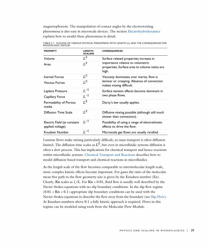
In general, as the length scale (L) of the fluid flow is reduced, properties that scale with the surface area of the system become comparatively more important than those that scale with the volume of the flow (see Table 2-1). This is apparent in the fluid flow itself as the viscous forces, which are generated by shear over the isovelocity surfaces (scaling as L2), dominate over the inertial forces (which scale volumetrically as L3). The Reynolds number (Re), which characterizes the ratio of these two forces, is typically low, so the flow is laminar. In many cases the creeping (Stokes) flow regime applies ( ). The section Single-Phase Flow describes microfluidic fluid flows in greater detail.

When multiple phases are present surface tension effects become important relative to gravity and inertia at small length scales. The Laplace pressure, capillary force, and Marangoni forces all scale as 1/L. The section Multiphase Flow gives more information on modeling flows involving several phases.

Flow through porous media can also occur on microscale geometries. Because the permeability of a porous media scales as L2 (where L is the average pore radius) the flow is often friction dominated when the pore size is in the micron range and Darcy’s law can be used. For intermediate flows this module also provides a physics interface to model flows where Brinkman equation is appropriate. For more information see Porous Media Flow.

At the microscale a range of electrohydrodynamic effects can be exploited to influence the fluid flow. The electric field strength for a given applied voltage scales as 1/L, making it easier to apply relatively large fields to the fluid with moderate voltages. In electroosmosis the uncompensated ions in the charged electric double layer (EDL) present on the fluid surfaces are moved by an electric field, causing a net fluid flow. Electrophoretic and dielectrophoretic forces on charged or polarized particles in the fluid can be used to induce particle motion, as can diamagnetic forces in the case of

Re 1«

2 : M I C R O F L U I D I C M O D E L I N G

magnetophoresis. The manipulation of contact angles by the electrowetting phenomena is also easy in microscale devices. The section Electrohydrodynamics explains how to model these phenomena in detail.

Laminar flows make mixing particularly difficult, so mass transport is often diffusion limited. The diffusion time scales as L2, but even in microfluidic systems diffusion is often a slow process. This has implications for chemical transport and hence reactions within microfluidic systems. Chemical Transport and Reactions describes how to model diffusion-based transport and chemical reactions in microfluidics.

As the length scale of the flow becomes comparable to intermolecular length scale, more complex kinetic effects become important. For gases the ratio of the molecular mean free path to the flow geometry size is given by the Knudsen number (Kn). Clearly, Kn scales as 1/L. For Kn < 0.01, fluid flow is usually well described by the Navier-Stokes equations with no-slip boundary conditions. In the slip flow regime (0.01 < Kn < 0.1) appropriate slip boundary conditions can be used with the Navier-Stokes equations to describe the flow away from the boundary (see Slip Flow). At Knudsen numbers above 0.1 a fully kinetic approach is required. Flows in this regime can be modeled using tools from the Molecular Flow Module.

TABLE 2-1: SCALING OF VARIOUS PHYSICAL PHENOMENA WITH LENGTH (L) AND THE CONSEQUENCES FOR MICROFLUIDIC DEVICES

PROPERTY LENGTH SCALING

CONSEQUENCES

Volume L3 Surface related properties increase in importance relative to volumetric properties, Surface area to volume ratios are high.

Area L2

Inertial Forces L3 Viscosity dominates over inertia, flow is laminar or creeping. Absence of convection makes mixing difficult.

Viscous Forces L2

Laplace Pressure L−1 Surface tension effects become dominant in two phase flows.Capillary Force L−1

Permeability of Porous media

L2 Darcy’s law usually applies.

Diffusion Time Scale L2 Diffusive mixing possible (although still much slower than convection).

Electric Field (at constant applied voltage)

L−1 Possibility of using a range of electrokinetic effects to drive the flow.

Knudsen Number L−1 Microscale gas flows are usually rarefied.

P H Y S I C S A N D S C A L I N G I N M I C R O F L U I D I C S | 29

30 | C H A P T E R

The next section describes the importance of Dimensionless Numbers in Microfluidics, which are frequently used in transport equations.

The Free Molecular Flow and Transitional Flow interfaces are available in the Molecular Flow Module.

The Physics Interfaces and Building a COMSOL Multiphysics Model in the COMSOL Multiphysics Reference Manual


D imen s i o n l e s s Numbe r s i n M i c r o f l u i d i c s

Information about the dominant physics in a microfluidics problem is contained in many of the dimensionless numbers that are used to characterize the flow. When using the finite element method, dimensionless numbers defined on the element or “cell” level can contain important information about the numerical stability of the problem (the term “cell” is carried over from the finite volume method in this context). This section includes information about the dimensionless numbers that are relevant to microfluidic flows.

In this section:

• Dimensionless Numbers Important for Solver Stability

• Other Dimensionless Numbers

Dimensionless Numbers Important for Solver Stability

When solving a microfluidics problem numerically there are two critical dimensionless numbers to consider in terms of solver stability. These numbers are:

• The Reynolds number (Re)

• The Peclet number (Pe)

Each of these numbers is defined in Table 2-2. Both the Reynolds number and the Peclet number are associated with the relative importance of convective terms in the corresponding partial differential equation. The Peclet number describes the importance of convection in relation to diffusion (for either heat or mass transfer), and the Reynolds number describes the importance of the “convective” inertia term in relation to viscosity in the Navier-Stokes equations themselves.

Both the Reynolds number and the Peclet number can be defined on the “cell” or element level. As they are defined in COMSOL Multiphysics numerical instabilities can arise when the cell Reynolds or Peclet number is greater than one. These instabilities are usually manifested as spurious oscillations in the solution. Taking the Peclet

D I M E N S I O N L E S S N U M B E R S I N M I C R O F L U I D I C S | 31

32 | C H A P T E R

number as an example, oscillations can occur when the cell Peclet number is greater than one in the following circumstances:

• A Dirichlet boundary condition can lead to a solution containing a steep gradient near the boundary, forming a boundary layer. If the mesh cannot resolve the boundary layer, this creates a local disturbance.

• A space-dependent initial condition that the mesh does not resolve can cause a local initial disturbance that propagates through the computational domain.

• A small initial diffusion term close to a nonconstant source term or a nonconstant Dirichlet boundary condition can result in a local disturbance.

In theory the grid can be refined to bring the cell Reynolds or Peclet number below one, although this is often impractical for many problems. Several stabilization techniques are included, which enable problems with larger cell Reynolds or Peclet numbers to be solved. At the crudest level additional numerical diffusion can be added to the problem to improve its stability. This is achieved by selecting Isotropic Diffusion under Inconsistent Stabilization for any physics interface.

This method is termed “inconsistent” as a solution to the problem without numerical diffusion is not necessarily a solution to the problem with diffusion. COMSOL Multiphysics also has consistent stabilization options. A consistent stabilization technique reduces the numerical diffusion added to the problem as the solution approaches the exact solution. Both streamline diffusion and crosswind diffusion are available. Streamline diffusion adds numerical diffusion along the direction of the flow velocity (that is, the diffusion is parallel to the streamlines). Crosswind diffusion adds diffusion in the direction orthogonal to the velocity.

Generally it is best to use consistent stabilization where possible. If convergence problems are still encountered, inconsistent stabilization can be used with a parametric or time-dependent solver that slowly eliminates this term.

The stabilization options are visible when the Show button ( ) is clicked and Stabilization is selected.

• Stabilization and Numerical Stabilization in the COMSOL Multiphysics Reference Manual

• Other Dimensionless Numbers


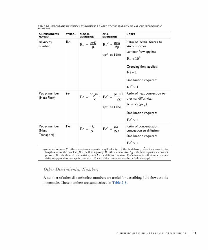
Other Dimensionless Numbers

A number of other dimensionless numbers are useful for describing fluid flows on the microscale. These numbers are summarized in Table 2-3.

TABLE 2-2: IMPORTANT DIMENSIONLESS NUMBERS RELATED TO THE STABILITY OF VARIOUS MICROFLUIDIC PROBLEMS.

DIMENSIONLESS NUMBER

SYMBOL GLOBAL DEFINITION

CELL DEFINITION

NOTES

Reynolds number

Re

spf.cellRe

Ratio of inertial forces to viscous forces.

Laminar flow applies:

Creeping flow applies:

Stabilization required:

Peclet number (Heat Flow)

Pe

spf.cellPe

Ratio of heat convection to thermal diffusivity,

.


Peclet number (Mass Transport)

Pe Ratio of concentration convection to diffusion.


Symbol definitions: v is the characteristic velocity or cell velocity, r is the fluid density, L is the characteristiclength scale for the problem, μ is the fluid viscosity, h is the element size, cp is the heat capacity at constantpressure, κ is the thermal conductivity, and D is the diffusion constant. For anisotropic diffusion or conduc-tivity an appropriate average is computed. The variables names assume the default name spf.

Re ρvLμ-----------= Rec ρvh

2μ----------=

Re 103<

Re 1«

Rec 1>

PeρcpvL

κ-----------------= Pec ρcpvh

2κ----------------=

α κ ρcp( )⁄=

Pec 1>

Pe vLD-------= Pec vh

2D--------=

Pec 1>


34 | C H A P T E R

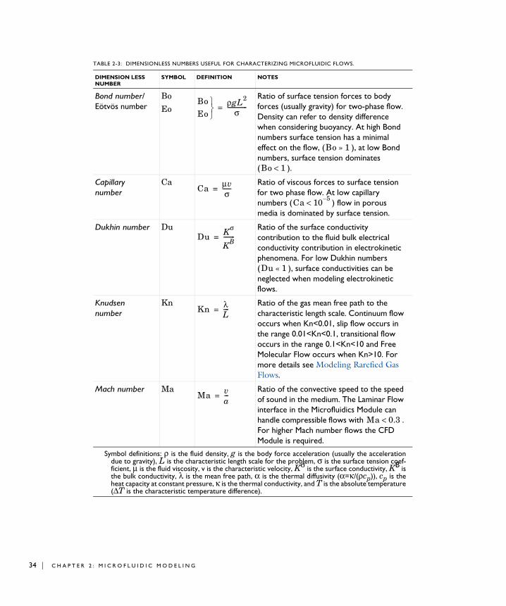
TABLE 2-3: DIMENSIONLESS NUMBERS USEFUL FOR CHARACTERIZING MICROFLUIDIC FLOWS.

DIMENSION LESS NUMBER

SYMBOL DEFINITION NOTES

Bond number/ Eötvös number

Bo

Eo

Ratio of surface tension forces to body forces (usually gravity) for two-phase flow. Density can refer to density difference when considering buoyancy. At high Bond numbers surface tension has a minimal effect on the flow, ( ), at low Bond numbers, surface tension dominates ( ).

Capillary number

Ca Ratio of viscous forces to surface tension for two phase flow. At low capillary numbers ( ) flow in porous media is dominated by surface tension.

Dukhin number Du Ratio of the surface conductivity contribution to the fluid bulk electrical conductivity contribution in electrokinetic phenomena. For low Dukhin numbers ( ), surface conductivities can be neglected when modeling electrokinetic flows.

Knudsen number

Kn Ratio of the gas mean free path to the characteristic length scale. Continuum flow occurs when Kn<0.01, slip flow occurs in the range 0.01<Kn<0.1, transitional flow occurs in the range 0.1<Kn<10 and Free Molecular Flow occurs when Kn>10. For more details see Modeling Rarefied Gas Flows.

Mach number Ma Ratio of the convective speed to the speed of sound in the medium. The Laminar Flow interface in the Microfluidics Module can handle compressible flows with . For higher Mach number flows the CFD Module is required.

Symbol definitions: ρ is the fluid density, g is the body force acceleration (usually the accelerationdue to gravity), L is the characteristic length scale for the problem, σ is the surface tension coef-ficient, μ is the fluid viscosity, v is the characteristic velocity, Kσ is the surface conductivity, KB isthe bulk conductivity, λ is the mean free path, α is the thermal diffusivity (α=κ/(ρcp)), cp is theheat capacity at constant pressure, κ is the thermal conductivity, and T is the absolute temperature(ΔT is the characteristic temperature difference).

BoEo

ρgL2

σ--------------=

Bo 1»

Bo 1<

Ca μvσ------=

Ca 10 5–<

Du Kσ

KB--------=

Du 1«

Kn λL----=

Ma va---=

Ma 0.3<


Marangoni number

Mg Ratio of thermal surface tension forces to viscous forces. In the low Marangoni number range ( ) viscous forces dominate over surface tension gradients.

Ohnesorge /Laplace /Surataman numbers

Oh

La

Su

Relates the inertial and surface tension forces to the viscous forces. Used to describe the breakup of liquid jets and sheets: at low Ohnesorge and Reynolds numbers the Rayleigh instability occurs, at high Ohnesorge and Reynolds numbers atomization occurs.

Weber number We Ratio of inertial forces to surface tension forces. For small Weber numbers ( ) surface tension dominates the flow.

TABLE 2-3: DIMENSIONLESS NUMBERS USEFUL FOR CHARACTERIZING MICROFLUIDIC FLOWS.

DIMENSION LESS NUMBER

SYMBOL DEFINITION NOTES

Symbol definitions: ρ is the fluid density, g is the body force acceleration (usually the accelerationdue to gravity), L is the characteristic length scale for the problem, σ is the surface tension coef-ficient, μ is the fluid viscosity, v is the characteristic velocity, Kσ is the surface conductivity, KB isthe bulk conductivity, λ is the mean free path, α is the thermal diffusivity (α=κ/(ρcp)), cp is theheat capacity at constant pressure, κ is the thermal conductivity, and T is the absolute temperature(ΔT is the characteristic temperature difference).

Mg dσdT--------LΔT

μα------------=

Mg 1000«

Oh μρσL---------------=

LaSu

1

Oh2-----------=

We ρv2Lσ

-------------=We 1«


36 | C H A P T E R

Mode l i n g M i c r o f l u i d i c F l u i d F l ow s

This section describes the modeling of fluid flows with the Navier Stokes or Stokes equations (the section Modeling Rarefied Gas Flows gives details on how to model rarefied flows). The following topics are covered:

• Selecting the Right Physics Interface

• Single-Phase Flow

• Multiphase Flow

• Porous Media Flow

• The Relationship Between the Physics Interfaces

Selecting the Right Physics Interface

COMSOL Multiphysics has a range of physics interfaces to use for fluid flow in a variety of circumstances. Often the selection of a particular physics interface implies certain assumptions about the equations of flow. If it is known in advance which assumptions are valid, then the appropriate physics interface can be added. However, when the flow type is unclear from the outset, or if it is difficult to reach a solution easily, starting with a simplified model and adding complexity subsequently is often a good approach. Using this approach the results of a simulation are tested against the underlying assumptions and against experimental results and the simulation can then be refined if necessary. For complex models it is often beneficial to take this approach even when the fluid flow is well characterized from the outset because a model with simplifying assumptions can be easier to solve initially. The solution process can then be fine-tuned for the more complex problem. Typically The Laminar Flow Interface is a good starting point for many problems.

The following sections describe the options available for simulating Single-Phase Flow, Multiphase Flow, and Porous Media Flow.

• Building a COMSOL Multiphysics Model in the COMSOL Multiphysics Reference Manual

• Modeling Rarefied Gas Flows


Single-Phase Flow

The Fluid Flow>Single-Phase Flow branch ( ) when adding a physics interface includes the Laminar and Creeping Flow interfaces.

The Laminar Flow Interface ( ) is used primarily to model slow-moving flow in environments without sudden changes in geometry, material distribution, or temperature. The Navier-Stokes equations are solved without a turbulence model. laminar flow typically occurs at Reynolds numbers less than 1000. By default the flow is incompressible (see Figure 2-1).

The Creeping Flow Interface ( ) uses the same equations as the Laminar Flow interface with the additional assumption that the contribution of the inertia term is negligible. This is often referred to as Stokes flow and is appropriate for use when viscous flow is dominant, which is often the case in microfluidics applications. Creeping flow applies when the Reynolds number is much less than one. A creeping flow problem is significantly simpler to solve than a laminar flow problem — so it is best to make this assumption explicitly if it applies. By default the flow is incompressible (see below).

For both physics interfaces several additional options are available.

S H A L L O W C H A N N E L A P P R O X I M A T I O N

Often you might want to simplify long, narrow channels by modeling them in 2D. The Use Shallow Channel Approximation option is useful as it includes a drag term to approximate the added affects given by thinness of the gap between one set of boundaries in comparison to the others.

C O M P R E S S I B L E F L O W

For compressible flow it is important that the density and any mass balances are well defined throughout the domain. Choosing to model incompressible flow simplifies the equations to be solved and decreases solution times. Most gas flows should be modeled as compressible flows; however, liquid flows can usually be treated as incompressible.

By selecting the Neglect Inertial Form (Stokes Flow) check-box, on the Settings window for Laminar Flow quickly convert a Laminar Flow interface into a Creeping Flow interface.

M O D E L I N G M I C R O F L U I D I C F L U I D F L O W S | 37

38 | C H A P T E R

N O N - N E W T O N I A N F L O W

The physics interfaces also allow for easy definition of non-Newtonian fluid flow through access to the dynamic viscosity in the Navier-Stokes equations. The fluid can be modeled using the power law and Carreau models or by means of any expression that describes the dynamic viscosity appropriately.

Both physics interfaces also include a feature to compute a laminar velocity profile at arbitrarily shaped inlets and outlets, which makes models much easier to set up.

Figure 2-1: The Settings window for Laminar Flow. Model incompressible or compressible (Ma<0.3) flow, and Stokes flow. Combinations are also possible.


Multiphase Flow

The Multiphase Flow branch ( ) enables the modeling of multiphase flows. These physics interfaces are included:

• The Laminar Two-Phase Flow, Level Set Interface ( ) (available under the Two-Phase Flow, Level Set branch ( )).

• The Laminar Two-Phase Flow, Phase Field Interface ( ) (available under the Two-Phase Flow, Phase Field branch ( )).

• The Laminar Two-Phase Flow, Moving Mesh Interface ( ) (available under the Two-Phase Flow, Moving Mesh branch ( )).

The Two-Phase Flow interfaces can add surface tension forces (including the Marangoni effect) at the two fluid interface(s). A library of surface tension coefficients between some common substances is available.

For problems involving topological changes (for example, jet breakup), use either the Level Set or Phase Field interfaces. These techniques use an auxiliary function (the level set and phase field functions, respectively) to track the location of the interface, which is necessarily diffuse. The Level Set interface does not include surface tension force per default, and is recommended for use in larger scale problems with larger velocities, or when the effects of the gradient of the surface tension coefficient are relevant. The phase field method is physically motivated and is usually more numerically stable than the level set method. It is can also be extended to more phases and is compatible with fluid-structure interactions (requires the MEMS Module or the Structural Mechanics Module).

The moving mesh method represents the interface as a boundary condition along a line or surface in the geometry. Because the physical thickness of phase boundaries is usually very small, for most practical meshes The Laminar Two-Phase Flow, Moving Mesh Interface describes the two-phase boundary the most accurately. However, it cannot accommodate topological changes in the boundary.

Switch between the Two-Phase Flow, Level Set interface and the Two-Phase

Flow, Phase Field interface by selecting one or other from a list available in both interfaces. This is useful if you are not sure which provides the best solution.


40 | C H A P T E R

For all the Two-Phase Flow interfaces, compressible flow is possible to model at speeds of less than 0.3 Mach. You can also choose to model incompressible flow by simplifying the equations to be solved. Stokes’ law is also an option.

In each physics interface, the density and viscosity are specified for both fluids. You can easily use non-Newtonian models for any of the two fluids, based on the power law, the Carreau model, or using an arbitrary user-defined expression.

It is often advantageous to use more than one of these techniques to solve a problem — for example, a level set model for jet breakup could be checked prior to breakup by a moving mesh model to ensure that the surface tension is captured accurately by the diffuse interface.

Porous Media Flow

The Porous Media and Subsurface Flow branch ( ) has the physics interfaces to model flow in porous media. The flow can be modeled by Darcy’s Law or the Brinkman Equations interfaces. Additionally the Brinkman equations can be combined with laminar flow in the Free and Porous Media Flow interface.

D A R C Y ’ S L A W

The Darcy’s Law Interface ( ) is used to model fluid movement through interstices in a porous medium in the case where the fluid viscosity dominates over its inertia. Together with the continuity equation and the equation of state for the pore fluid (or gas) Darcy’s law is used to model low velocity flows, for which the pressure gradient is the dominant driving force (typically when the Reynolds number of the flow is less than one). The penetration of reacting gases in a tight catalytic layer, such as a washcoat or membrane, is an example in which Darcy’s law applies. Often Darcy’s law is applicable for microfluidic applications, as it is appropriate for the limit of small pore size.

Under the Mathematics>Moving Interface branch ( ) when adding an interface, The Level Set Interface ( ) and The Phase Field Interface ( ) are available in a form uncoupled with the equations of flow. These interfaces can be used to model phenomena in which other factors dominate over the fluid flow, such as some forms of phase separation.


B R I N K M A N E Q U A T I O N S

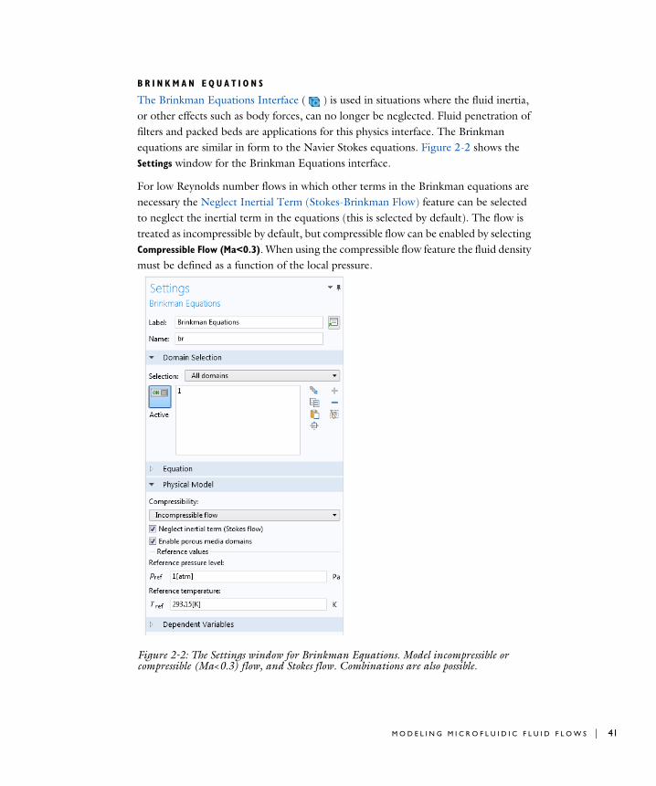
The Brinkman Equations Interface ( ) is used in situations where the fluid inertia, or other effects such as body forces, can no longer be neglected. Fluid penetration of filters and packed beds are applications for this physics interface. The Brinkman equations are similar in form to the Navier Stokes equations. Figure 2-2 shows the Settings window for the Brinkman Equations interface.

For low Reynolds number flows in which other terms in the Brinkman equations are necessary the Neglect Inertial Term (Stokes-Brinkman Flow) feature can be selected to neglect the inertial term in the equations (this is selected by default). The flow is treated as incompressible by default, but compressible flow can be enabled by selecting Compressible Flow (Ma<0.3). When using the compressible flow feature the fluid density must be defined as a function of the local pressure.

Figure 2-2: The Settings window for Brinkman Equations. Model incompressible or compressible (Ma<0.3) flow, and Stokes flow. Combinations are also possible.


42 | C H A P T E R

F R E E A N D P O R O U S M E D I A

The Free and Porous Media Flow Interface ( ) has predefined couplings between the Brinkman Equations interface and the Laminar Flow interface. Porous regions of the models are included by adding a Porous Matrix Properties node with the appropriate selections to the model. The default Fluid Properties node can then be used to define regions of free laminar flow. This physics interface has all the options from both The Laminar Flow Interface and The Brinkman Equations Interface. An example application area for this physics interface would be a catalytic converter.

It should be noted that if the porous medium is large in comparison to the free channel, and the results in the region of the interface are not of interest, then it is possible to manually couple a Fluid Flow interface to the Darcy’s Law interface. This makes the model computationally cheaper.

The Relationship Between the Physics Interfaces

Several of the physics interfaces vary only by one or two default settings (see Table 2-4, Table 2-5) in the Physical Model section, which are selected either from a check box or list. For the Single-Phase Flow branch, the Laminar Flow and Creeping Flow interfaces have the same Name (spf), and this is the same for two of the Two-Phase Flow interfaces. In the Porous Media Flow branch the Free and Porous Media Flow interface combines a Laminar Flow interface with a Brinkman Equations interface (see Table 2-6).

TABLE 2-4: THE SINGLE-PHASE FLOW PHYSICAL MODEL DEFAULT SETTINGS

PHYSICS INTERFACE LABEL

NAME COMPRESSIBILITY NEGLECT INERTIAL TERM (STOKES FLOW)

Laminar Flow spf Compressible flow (Ma<0.3)

None

Creeping Flow spf Compressible flow (Ma<0.3)

Stokes Flow

TABLE 2-5: TWO-PHASE FLOW PHYSICAL MODEL DEFAULT SETTINGS


NAME MULTIPHASE FLOW MODEL

COMPRESSIBILITY NEGLECT INERTIAL TERM (STOKES FLOW)

Laminar, Two-Phase Flow, Level Set

tpf Two phase flow, level set

Incompressible flow

None


Laminar, Two-Phase Flow, Phase Field

tpf Two phase flow, phase field

Incompressible flow

None

Laminar, Two-Phase Flow, Moving Mesh

spf not applicable Incompressible flow

None

TABLE 2-6: THE POROUS MEDIA FLOW DEFAULT SETTINGS


NAME COMPRESSIBILITY NEGLECT INERTIAL TERM

PORE SIZE

Darcy's Law dl n/a n/a Low porosity and low permeability, slow flow

Brinkman Equations

br Incompressible flow

Yes - Stokes-Brinkman

High permeability and porosity, faster flow

Free and Porous Media Flow

fp Incompressible flow

Not selected High permeability and porosity, fast flow

TABLE 2-5: TWO-PHASE FLOW PHYSICAL MODEL DEFAULT SETTINGS


NAME MULTIPHASE FLOW MODEL

COMPRESSIBILITY NEGLECT INERTIAL TERM (STOKES FLOW)


44 | C H A P T E R

Mode l i n g Coup l e d Phenomena i n M i c r o f l u i d i c s

In this section:

• Chemical Transport and Reactions

• Electrohydrodynamics

• Heat Transfer

• Coupling to Other Physics Interfaces

Chemical Transport and Reactions

In the Microfluidics Module, The Transport of Diluted Species Interface ( ) and The Transport of Diluted Species in Porous Media Interface ( ) are available for modeling the transport of chemical species and ions. The assumption in these physics interfaces is that one component, a solvent, is present in excess (typically more than 90 mol%). This means that the mixture properties, such as density and viscosity, are independent of concentration. To model concentrated species, the Chemical Reaction Engineering Module is recommended in addition to the Microfluidics Module.

By default the Transport of Diluted Species interface accounts for the diffusion of species by Fick’s law and convection due to bulk fluid flow (see Figure 2-3). The fluid velocity field can be coupled from another physics interface (for example, Laminar Flow) by means of a domain level model input. The migration of ionic species in an electric field can also be added by selecting the appropriate check box in the Settings window for the physics interface—in this case an additional Electrostatics interface is usually coupled into the problem by an additional model input.

Chemical reactions can be added to the physics interface at the domain level by the Reactions node, which requires the Chemical Reaction Engineering Module. This allows you to specify expressions for the consumption or production of species in terms

See The AC/DC Interfaces in the COMSOL Multiphysics Reference Manual for details, including theory, about The Electrostatics Interface and The Magnetic Fields Interface, which are included with the basic COMSOL Multiphysics license and discussed in this section.


of their concentration, the concentration of other species and other model parameters, such as the temperature.

Figure 2-3: The Settings window for Transport of Diluted Species, with Convection selected as the Transport Mechanism by default.

S T A B I L I Z A T I O N S E T T I N G S F O R D I L U T E D S P E C I E S T R A N S P O R T

For some laminar flow problems it can be useful to change the settings for the dilute species transport stabilization. To do this, click the Show button ( ) and select Stabilization. A Consistent stabilization section is now visible in the Transport of Diluted species settings, and in some cases it can be desirable to change the settings for the crosswind diffusion. By default the Crosswind diffusion type is set to Do Carmo and

Galeão. This type of crosswind diffusion reduces undershoot and overshoot to a minimum but can in rare cases give equations systems that are difficult to fully converge. The alternative option, Codina is less diffusive and so should be used if the species transport is highly convective, or if convergence problems occur. This option can result in more undershoot and overshoot and is also less effective for anisotropic meshes. The Codina option activates a text field for the Lower gradient limit glim (SI unit: mol/m4). It defaults to 0.1[mol/m^3)/tds.helem, where tds.helem is the local element size.

M O D E L I N G C O U P L E D P H E N O M E N A I N M I C R O F L U I D I C S | 45

46 | C H A P T E R

For both consistent stabilization methods, the Equation residual can also be changed. Approximate residual is the default setting and it means that derivatives of the diffusion tensor components are neglected. This setting is usually accurate enough and is faster to compute. If required, select Full residual instead.

Electrohydrodynamics

Electrohydrodynamics is a general term describing phenomena that involve the interaction between solid surfaces, ionic solutions, and applied electric and magnetic fields. Electrohydrodynamics is frequently employed in microfluidic devices to manipulate fluids and move particles for sample handling and chemical separation.

Electrokinetics refers to a range of fluid flow phenomena involving electric fields. These include electroosmosis, electrothermal effects, electrophoresis and dielectrophoresis. Electrosmosis describes the motion of fluids induced by the forces on the charged EDLs at the surfaces of the fluid. Electrothermal effects occur in a conductive fluid where the temperature is modified by Joule heating from an AC electric field. This creates variations in conductivity and permittivity and thus Coulomb and dielectric body forces. Electrophoresis and dielectrophoresis describe the motion of charged and polarized particles in a non-uniform AC or DC applied field.

Magnetohydrodynamics refers to fluid flow phenomena involving magnetic fields. Magnetophoresis is the motion of diamagnetic particles in a nonuniform magnetic field and is commonly used for magnetic bead separation.

Table 2-7 summarizes these categories. Although these examples describe specific multiphysics couplings, COMSOL Multiphysics is not limited to these cases—for


example, it is possible to include both magnetic and electric fields to simulate electromagnetophoresis.

E L E C T R O O S M O S I S

When a polar liquid (such as water) and a solid surface (such as glass or a polymer-based substrate) come into contact, charge transfer occurs between the surface and the electrolytic solution. At finite temperature the charges on the surface are not screened perfectly by the ions in the liquid and a finite thickness electric double layer (EDL) or Debye layer develops. Electroosmosis is the process by which motion is induced in a liquid due to the body force acting on the EDL in an electric field.

A complete model of the system includes the space charge layer explicitly. The electric potential is the solution of a nonlinear partial differential equation, the Poisson-Boltzmann equation, which can be solved by coupling an Electrostatics interface to a Transport of Diluted Species interface (with migration enabled) for the ion species. The software then computes the forces on the fluid and a further coupled Laminar Flow or Creeping Flow interface is used to compute the overall fluid flow. In practice this approach is only possible for nanoscale channels—as typically the EDL thickness is 1-10 nm.

The Poisson Boltzmann equation is sometimes linearized—this is referred to as the Debye-Hückel approximation which applies when , where ζ is the potential at the surface of the moving volume of fluid (the zeta potential). At room temperature

TABLE 2-7: ELECTROHYDRODYNAMIC PHENOMENA

TYPE OF FIELD/FORCE DC AC

ELECTRIC FIELD (ELECTROKINETICS)

Surface force on fluid Electroosmosis AC electroosmosis

Force on suspended particles Electrophoresis / Dielectrophoresis

AC Electrophoresis /AC Dielectrophoresis

Body force on fluid - Electrothermal

Magnetic Field

Force on suspended particles Magnetophoresis -

See The AC/DC Interfaces in the COMSOL Multiphysics Reference Manual for details, including theory, about The Electrostatics Interface and The Magnetic Fields Interface, which are included with the basic COMSOL license and discussed in this section.

zeζ kBT«


48 | C H A P T E R

this corresponds to the limit mV. Note that there is a layer of immobile ions trapped adjacent to the surface (the Stern Layer, which is of order one hydrated ion radius thick) with an associated volume of immobile fluid; this means that ζ is not simply the wall potential. ζ is usually determined experimentally from electroosmotic flow measurements.

The Poisson-Boltzmann equation has a characteristic length scale — the Debye length, λD:

where kB is Boltzmann’s constant, T is the temperature, z is the ion’s valance number, e is the electron charge, and c∞ is the ion’s molar concentration in the bulk solution. When the Debye length is small compared to the channel thickness, the electroosmotic flow velocity can be modeled by the Helmholtz-Smoluchowski equation:

where E is the applied electric field and μ is the liquid’s dynamic viscosity. From this equation, the electroosmotic mobility is naturally defined as:

(2-1)

The Laminar Flow and Creeping Flow interfaces include a wall boundary condition option for an Electroosmotic Velocity boundary condition. This enables you to specify the external electric field (which can be manually specified or coupled from an Electrostatics interface) and the electroosmotic mobility to define an electroosmotic flow.

Further details of the theory of electroosmosis can be found in Ref. 1 and Ref. 2.

A C E L E C T R O O S M O S I S

Because an alternating electric field does not generate a net force on the EDL, AC electroosmosis is not used for fluid transport in microfluidics. However, the back-and-forth movements an AC field generates are useful for mixing purposes. To model AC electroosmotic flow when the frequency of the electric field is sufficiently low, the same approaches can be taken as for DC electroosmosis. An Electrostatics interface should still be used to calculate the electric field, but when this is coupled into other physics interfaces, the AC dependence should be explicitly added using an

ζ 26«

λDεkBT

2z2e2c∞

---------------------=

ueoεζμ-----E=

μeoεζμ-----=


expression. With increasing frequency, AC electroosmosis becomes less important so this approach is valid for most practical examples.

E L E C T R O P H O R E S I S

Electrophoresis describes the motion of charged particles or molecules suspended in a liquid due to an applied electric field.

In COMSOL Multiphysics it is easy to calculate the electrophoretic velocity for spherical particles for the cases when the Debye length is much smaller or much larger than the particle size. If the surface conductivity of the particle can be neglected (this is sometimes referred to as the limit or small Dukhin number) the electrophoretic velocity (the particle velocity relative to the bulk flow) is given by:

where a is the radius of the particle, E is the electric field, and f(a/λD) is known as Henry’s function (note that f(a/λD) is often written as f(κa) where κ=1/λD). Henry’s function takes the value of 1 in the limiting case where (often known as the Hückel approximation) and 3/2 in the case where (this is equivalent to Equation 2-1 and is referred to as the Smoluchowski approximation). Note that if λD is large compared to the fluid volume, the charge is effectively unscreened and the electric force is simply that due to the charge on the molecule. The following result is obtained from the force balance between the Stokes drag and the electric force for an unscreened charged particle:

where q is the charge on the molecule and μ is the fluid viscosity. Further details of the theory of electroosmosis can be found in Ref. 2.

These velocity fields can be computed directly from an electric field calculated by the Electrostatics interface. If necessary the velocity can be added to the flow velocity field to compute the net particle velocity.

Electroosmotic Micromixer: Application Library path Microfluidics_Module/Micromixers/electroosmotic_mixer

uep23---μeof a

λD------- E=

a λD«

a λD»

uepq

6πμa--------------E=


50 | C H A P T E R

D I E L E C T R O P H O R E S I S

Dielectrophoresis (DEP) describes the motion of polarizable particles suspended in a fluid with an applied nonuniform electric field. The electric field induces a dipole moment on the particles, which in turn produces a net force. In the following discussion the general case of AC electrophoresis is treated, which is more commonly used for practical reasons (see Ref. 1 for further details).

The time-dependent dielectrophoretic force acting on a particle in an applied field is given by (Ref. 1):

(2-2)

where εm and εp are the complex permittivities of the medium and the particle respectively, a is the radius of the particle’s equivalent homogeneous sphere and K(εm,εp) is the Clausius-Mossotti function. The complex permittivity, ε*, for an isotropic homogeneous dielectric is

where ε is the electric permittivity, σ is the electrical conductivity, and ω is the angular field frequency. The Clausius-Mossotti function is given by:

which depends on the particle’s complex permittivity, εp, and that of the medium, εm.

Taking the time average of Equation 2-2 gives the time averaged force:

By balancing this force with the Stokes drag force the dielectrophoretic velocity is obtained:

For a DC field these results can be applied if Erms=E is used.

FDEP

t( ) 2πεma3K εm εp,( )∇ E t( ) E t( )⋅( )=

ε∗ ε iσω----–=

K εm εp,( )εp ε– m

εp 2ε+ m----------------------=

FDEP

t( ) 2πεmr0Re K εm εp,( )( )∇ Erms Erms⋅( )=

uDEP

εmr0Re K εm εp,( )( )∇ Erms Erms⋅( )3μ

---------------------------------------------------------------------------------------------=


where μ is the dynamic viscosity.

The value of Erms can be computed from an Electrostatics interface in which the root mean square (RMS) voltages are applied as boundary conditions. The gradient of the field can then be computed term by term from the spatial derivatives of an expression for the dot product of the electric field with itself. Finally the dielectrophoretic velocity term can be added to the velocity field to compute the particle velocity field.

M A G N E T O P H O R E S I S

Particles with an induced or permanent magnetization can be moved relative to a fluid flow by the application of an external, inhomogeneous magnetic field. This process is analogous to dielectrophoresis and is usually termed magnetophoresis. In the case of a nonconducting particle, in a static, irrotational external applied field, Hext, the magnetophoretic force is given by (Ref. 1):

where μm and μp are the permeabilities of the medium and the particle respectively (usually μm =μ0), a is the radius of the particle’s equivalent homogeneous sphere and K(μm,μp) is the Clausius-Mossotti function. Note that the external magnetic field, Hext, should be distinguished from the local field H which includes contributions from the particle itself. In this case the Clausius-Mossotti function is given by:

By balancing this force with the Stokes drag force the magnetophoretic velocity is obtained:

where μ is the dynamic viscosity.

The value of Hext can be computed from a Magnetic Fields or a Magnetic Fields, No Currents interface.

FMAP 2πμmK μm μp,( )a3 Hext Hext⋅( )∇=

K μm μp,( )μp μm–

μp 2μm+------------------------=

uMAP

μmr0K μm μp,( )∇ Hext Hext⋅( )3μ

-------------------------------------------------------------------------------=

The Magnetic Fields, No Currents interface requires the AC/DC Module.


52 | C H A P T E R

The gradient of the field can then be computed term by term from the spatial derivatives of an expression for the dot product of the magnetic field with itself. Finally the magnetophoretic velocity term can be added to the velocity field to compute the particle velocity field.

E L E C T R O T H E R M A L L Y - D R I V E N F L O W

Electrothermal body forces arise from electrically generated, nonuniform Joule heating, which creates variations in conductivity and permittivity and thus Coulomb and dielectric body forces. It is possible to determine the resulting fluid motion by solving the Navier-Stokes equations with an additional electrothermal body force term. The electric field is once again assumed to be quasi-static and can be coupled in from an Electrostatics interface.

The electrothermal force is given by:

where σ is the conductivity, ε is the fluid’s permittivity, ω is the angular frequency of the electric field, and τ = ε/σ is the fluid’s charge-relaxation time. The electric-field vector E contains the amplitude and direction of the AC electric field but not its instantaneous value.

Because of the heating, ε and σ are temperature dependent, and their gradients are functions of the temperature gradient: ∇ε = (∂ε/∂T)∇T and ∇σ = (∂σ/∂T)∇T. With water, for example, the relative change rates for the permittivity and the conductivity are (1/ε)(∂ε/∂T) = −0.004 1/K and (1/σ)(∂σ/∂T) = 0.02 1/K, respectively.

E L E C T R O W E T T I N G

The contact angle of a two-fluid interface with a solid surface is determined by the balance of the forces at the contact point. The equilibrium contact angle, θ0, is given by Young’s equation:

The Magnetic Fields Interface in the COMSOL Multiphysics Reference Manual

F 12--- ∇σ

σ-------- ∇ε

ε-------+

E εE

1 ωτ( )2+

------------------------ 12--- E 2∇ε+⋅–=

γs1 σ+ 12 θ0cos γs2=


Here γs1 is the surface energy per unit area between fluid 1 and the solid surface, γs2 is the surface energy per unit area between fluid 2 and the solid surface, and σ12 is the surface tension at the interface between the two fluids.

In electrowetting the balance of forces at the contact point is modified by the application of a voltage between a conducting fluid and the solid surface. For many applications the solid surface consists of a thin dielectric deposited onto a conducting layer; this is often referred to as Electrowetting on Dielectric (EWOD). In this case, the capacitance of the dielectric layer dominates over the double layer capacitance at the solid-liquid interface (Ref. 3). The energy stored in the capacitor formed between the conducting liquid and the conducting layer in the solid reduces the effective surface energy of the liquid to which the voltage is applied. For the case when a voltage difference occurs between fluid 1 and the conductor beyond the dielectric Young’s equation is modified as follows:

Here ε is the permittivity of the dielectric, V is the potential difference applied, and df is the dielectric thickness. This equation can be rewritten as

(2-3)

Electrowetting can therefore be used to modify the contact angle dynamically by changing the applied voltage.

The EWOD applications can be modeled by using Equation 2-3 as an expression for the contact angle. This can simply be entered as the value of the contact angle in the Two-Phase Flow interface that is being used. Note that the software automatically handles a time varying voltage in this expression.

Heat Transfer

It is often necessary to consider the effect of heat flow and temperature dependent material properties (such as the viscosity or the surface tension) in microfluidic systems. The COMSOL Multiphysics base package includes physics interfaces for heat transfer

γs1εV2

2df----------– σ+

12θewcos γs2=

θewcos θ0cos εV2

2σ12df------------------+=

For step-by-step instructions, see Electrowetting Lens: Application Library path Microfluidics_Module/Two-Phase_Flow/electrowetting_lens.


54 | C H A P T E R

in incompressible fluids and solids. The Heat Transfer Module is required in addition to this module to model heat flow in compressible fluids and to include viscous heating terms. This section describes how to couple heat transfer to microfluidics models using the functionality available in the COMSOL Multiphysics base package and the Microfluidics Module.

The Heat Transfer interface includes the equations for heat transfer in both fluid and solid domains. To model a system consisting of both solid and liquid domains add a single Heat Transfer interface and then add nodes for Heat Transfer in Solids and Heat Transfer in Fluids with selections corresponding to the solid and fluid domains respectively. For a fluid domain the convective flow is coupled into domain by selecting the velocity field from a corresponding Laminar Flow or Creeping Flow interface.

The fluid domain models the heat transfer including both convection and conduction according to the equation:

where, ρ is the fluid density (SI unit: kg/m3), Cp is the specific heat capacity at constant pressure (SI unit: J/(kg·K)), T is absolute temperature (SI unit: K), u is the velocity vector (SI unit: m/s), q is the heat flux by conduction (SI unit: W/m2), and Q contains heat sources other than viscous heating (SI unit: W/m3). For a solid domain the following equation applies:

When using the heat transfer in solids and in fluids domain properties the software automatically includes the heat transfer between the solid and the fluid. It is important to include the correct thermal boundary conditions on regions where fluid flows into or out of a domain, typically a Temperature condition for an inlet and an Outflow condition for an outlet.

ρCp∂T∂t------- u ∇⋅( )T+ ∇ q⋅( )– Q+=

ρCp∂T∂t------- ∇ q⋅( )– Q+=

For a detailed discussion of the fundamentals of heat transfer, see Ref. 4. More details of the heat transfer capabilities can be found in The Heat Transfer Interfaces in the COMSOL Multiphysics Reference Manual.


Coupling to Other Physics Interfaces

The COMSOL Multiphysics software is not limited to the common couplings described in this chapter — there are many other phenomena that can be easily modeled in microfluidics. In many cases, physics interfaces can be coupled simply by entering expressions from one physics interface (such as the local temperature) into fields in another physics interface (for example in the Model Inputs section of a Fluid

Properties node). Additionally, COMSOL Multiphysics includes powerful coupling operators that enable physics interfaces to be linked by projections, extrusions, or scalar quantities such as integrals and global averages.

Component Couplings and Coupling Operators in the COMSOL Multiphysics Reference Manual


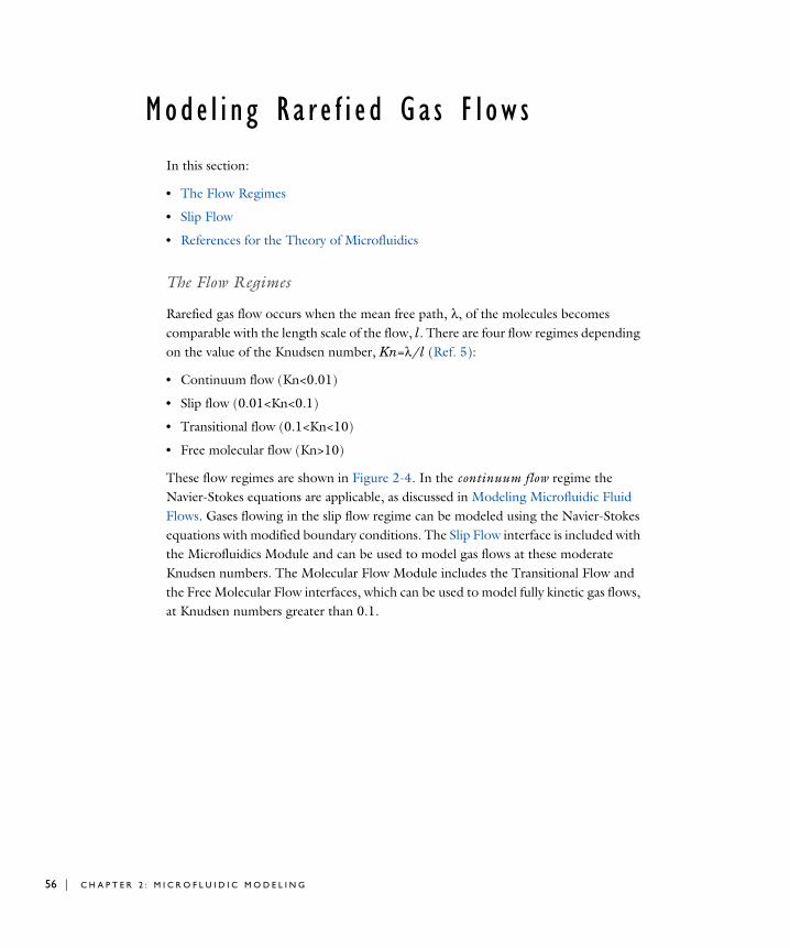
56 | C H A P T E R

Mode l i n g Ra r e f i e d Ga s F l ow s

In this section:

• The Flow Regimes

• Slip Flow

• References for the Theory of Microfluidics

The Flow Regimes

Rarefied gas flow occurs when the mean free path, λ, of the molecules becomes comparable with the length scale of the flow, l. There are four flow regimes depending on the value of the Knudsen number, Kn=λ/l (Ref. 5):

• Continuum flow (Kn<0.01)

• Slip flow (0.01<Kn<0.1)

• Transitional flow (0.1<Kn<10)

• Free molecular flow (Kn>10)

These flow regimes are shown in Figure 2-4. In the continuum flow regime the Navier-Stokes equations are applicable, as discussed in Modeling Microfluidic Fluid Flows. Gases flowing in the slip flow regime can be modeled using the Navier-Stokes equations with modified boundary conditions. The Slip Flow interface is included with the Microfluidics Module and can be used to model gas flows at these moderate Knudsen numbers. The Molecular Flow Module includes the Transitional Flow and the Free Molecular Flow interfaces, which can be used to model fully kinetic gas flows, at Knudsen numbers greater than 0.1.


Figure 2-4: A plot showing the main fluid flow regimes for rarefied gas flows. Different regimes are separated by lines of constant Knudsen numbers. The number density of the gas is normalized to the number density of an ideal gas at a pressure of 1 atmosphere and a temperature of 0 °C (n0).

Slip Flow

In the slip flow regime, the Navier-Stokes equations can still be used with modified boundary conditions to account for rarefaction effects close to the wall. A layer of rarefied gas with a size similar to the mean free path develops close to the wall—this is termed the Knudsen layer. The Navier-Stokes equations are not applicable in this layer, but the flow outside the layer can be described by extrapolating the bulk gas flow toward the wall and applying Maxwell’s slip boundary condition at the wall (Ref. 5). For thermal flows the von Smoluchowski temperature jump boundary condition must also be applied (Ref. 5).

To model flows in the slip flow regime use the Slip Flow interface. That physics interface can be used to model isothermal and non-isothermal flows with or without explicit modeling of thermal processes in adjacent solid domains. To model isothermal flows use the Temperature boundary condition on all external model surfaces, with the temperature set equal to the fluid temperature. The Slip Wall and External Slip Wall boundary conditions are used to model slip on interior and exterior model boundaries respectively. These boundary conditions include thermal creep or transpiration, viscous

Continuum flow

Slip flow

Transitional flow

Free molecular flow

M O D E L I N G R A R E F I E D G A S F L O W S | 57

58 | C H A P T E R

slip, and the von Smoluchowski temperature jump. The slip coefficients can be specified directly or by means of Maxwell’s model. For further details see The Slip Flow Interface and Theory for the Slip Flow Interface.

References for the Theory of Microfluidics

1. H. Bruus, Theoretical Microfluidics, Oxford University Press, 2008.

2. R.F. Probstein, Physicochemical Hydrodynamics: An Introduction, 2nd ed., Wiley-Interscience, 2003.

3. F. Mugele and J.C. Baret, “Electrowetting: from basics to applications”, J. Phys. Condens. Matter, vol. 17, pp. R705–R774, 2005.

4. F.P. Incropera and D.P. DeWitt, Fundamentals of Heat and Mass Transfer, 4th ed., John Wiley & Sons, 1996.

5. G. Kariadakis, A. Beskok, and N. Aluru, Microflows and Nanoflows, Springer Science and Business Media, 2005.

• The Temperature boundary condition is described for the Heat Transfer interface in the COMSOL Multiphysics Reference Manual.

• Slip Velocity


3

S i n g l e - P h a s e F l o w I n t e r f a c e s

There are several Fluid Flow interfaces available with the Microfluidics Module. These are grouped by type and found under the Fluid Flow>Single-Phase Flow branch ( ) when adding a physics interface. See Modeling Microfluidic Fluid Flows to help you select which physics interface to use.

In this chapter:

• The Laminar Flow and Creeping Flow Interfaces

• Theory for the Single-Phase Flow Interfaces

59

60 | C H A P T E R

Th e L am i n a r F l ow and C r e e p i n g F l ow I n t e r f a c e s

In this section:

• The Creeping Flow Interface

• The Laminar Flow Interface

In the COMSOL Multiphysics Reference Manual, see Table 2-3 for links to common sections such as Discretization, Consistent Stabilization, Inconsistent Stabilization, and Advanced Settings sections, all accessed by clicking the Show button ( ) and choosing the applicable option. You can also search for information: press F1 to open the Help window or Ctrl+F1 to open the Documentation window.

The Creeping Flow Interface

The Creeping Flow (spf) interface ( ) is used for simulating fluid flows at very low Reynolds numbers for which the inertial term in the Navier-Stokes equations can be neglected. Creeping flow, also referred to as Stokes flow, occurs in systems with high viscosity or small geometrical length scales (for example, in microfluidics and MEMS devices). The fluid can be compressible or incompressible, as well as Newtonian or non-Newtonian.

The equations solved by the Creeping Flow interface are the Stokes equations for conservation of momentum and the continuity equation for conservation of mass.

The Creeping Flow interface can be used for stationary and time-dependent analyses.

The main feature is the Fluid Properties node, which adds the Stokes equations and provides an interface for defining the fluid material and its properties. Except where noted below, see The Laminar Flow Interface for all other settings.

• Domain, Boundary, Pair, and Point Nodes for Single-Phase Flow


3 : S I N G L E - P H A S E F L O W I N T E R F A C E S

P H Y S I C A L M O D E L

By default, the Neglect inertial term (Stokes flow) check box is selected. If unchecked, the inertial terms are included in the computations.

D I S C R E T I Z A T I O N

By default, the Creeping Flow interface uses P2+P1 elements. Contrary to general laminar and turbulent single-phase flow simulations employing purely linear P1+P1 elements, P2+P1 elements are well suited for most creeping flow simulations but are not in general fully conservative. Full conservation properties and high accuracy is obtained by selecting P2+P2 or P3+P3 elements.

Note that P1+P1, P2+P2, and P3+P3 discretizations (the so-called equal order interpolations) require streamline diffusion to be active.

C O N S I S T E N T S T A B I L I Z A T I O N

This check box is selected by default and should remain selected for optimal performance. The consistent stabilization method does not perturb the original transport equation.

The Laminar Flow Interface

The Laminar Flow (spf) interface ( ) is used to compute the velocity and pressure fields for the flow of a single-phase fluid in the laminar flow regime. A flow remains laminar as long as the Reynolds number is below a certain critical value. At higher Reynolds numbers, disturbances have a tendency to grow and cause transition to turbulence. This critical Reynolds number depends on the model, but a classical example is pipe flow, where the critical Reynolds number is known to be approximately 2000.

• The Laminar Flow Interface


• Transport in an Electrokinetic Valve: Application Library path Microfluidics_Module/Fluid_Flow/electrokinetic_valve

• Controlled Diffusion Micromixer: Application Library path Microfluidics_Module/Micromixers/controlled_diffusion_micromixer

T H E L A M I N A R F L O W A N D C R E E P I N G F L O W I N T E R F A C E S | 61

62 | C H A P T E R

The physics interface supports incompressible flow, weakly compressible flow (the density depends on temperature but not on pressure), and compressible flow at low Mach numbers (typically less than 0.3). It also supports flow of non-Newtonian fluids.

The equations solved by the Laminar Flow interface are the Navier-Stokes equations for conservation of momentum and the continuity equation for conservation of mass.

The Laminar Flow interface can be used for stationary and time-dependent analyses. Time-dependent studies should be used in the high-Reynolds number regime as these flows tend to become inherently unsteady.

When the Laminar Flow interface is added, the following default nodes are also added in the Model Builder: Fluid Properties, Wall (the default boundary condition is No slip), and Initial Values. Other nodes that implement, for example, boundary conditions and volume forces, can be added from the Physics toolbar or from the context menu displayed when right-clicking Laminar Flow.

S E T T I N G S

The Label is the default physics interface name.

The Name is used primarily as a scope prefix for variables defined by the physics interface. Physics interface variables can be referred to using the pattern <name>.<variable_name>. In order to distinguish between variables belonging to different physics interfaces, the name string must be unique. Only letters, numbers, and underscores (_) are permitted in the Name field. The first character must be a letter.

The default Name (for the first physics interface in the model) is spf.

About the Physics Interface Label NamesThe label for a single-phase flow interface (the node name in the Model Builder) is dynamic and is reset according to the turbulence model and the neglect inertial term (Stokes flow) property set at the physics interface level. The availability also depends on the software license.

If the Neglect inertial term (Stokes flow) check box is selected, then the Label changes to Creeping Flow, which is the same Label that displays when that interface is added from the Model Wizard or Add Physics window.


CompressibilityDepending of the fluid properties and the flow regime, three options are available for the Compressibility option. In general the computational complexity increases from


Incompressible flow to Weakly compressible flow to Compressible flow (Ma<0.3) but the underlying hypotheses are increasingly more restrictive in the opposite direction.

When the Incompressible flow option (default) is selected, the incompressible form of the Navier-Stokes and continuity equations is applied. In addition, the fluid density is evaluated at the Reference pressure level defined in this section. The Reference

temperature is set to 293.15 K.

The Weakly compressible flow option models compressible flow when the pressure dependency of the density can be neglected. When selected, the compressible form of the Navier-Stokes and continuity equations is applied. In addition, the fluid density is evaluated at the Reference pressure level defined in this section.

When the Compressible flow (Ma<0.3) option is selected, the compressible form of the Navier-Stokes and continuity equations is applied. Ma < 0.3 indicates that the inlet and outlet conditions, as well as the stabilization, may not be suitable for transonic and supersonic flow. For more information, see The Mach Number Limit.

Neglect Inertial Term (Stokes Flow)For low Reynolds number flows, the inertial terms in the Navier-Stokes equations may be neglected.

Porous Media DomainsWith the addition of various modules, the Enable porous media domains check box is available. Selecting this option, a Fluid and Matrix Properties node, a Mass Source node, and a Forchheimer Drag subnode are added to the physics interface. These are described for the Brinkman Equations interface in the respective module’s documentation. The Fluid and Matrix Properties can be applied on all domains or on a subset of the domains.

Use Shallow Channel ApproximationFor 2D components, selecting the Use shallow channel approximation check box enables modeling of fluid flow in shallow channels in microfluidics applications. Such channels often have an almost rectangular cross section where the Channel thickness dz is much smaller than the channel width. Simple 2D components often fail to give correct results for this type of problems because they exclude the boundaries that have the greatest effect on the flow. The shallow channel approximation takes the effect of these boundaries into account by adding a drag term as a volume force to the momentum equation. The form of this term is

(3-1)Fμ 12 μu

dz2

--------–=


64 | C H A P T E R

where μ is the fluid’s dynamic viscosity, u is the velocity field, and dz is the channel thickness. This term represents the resistance that the parallel boundaries impose on the flow; however, it does not account for any changes in velocity due to variations in the cross-sectional area of the channel.

Reference valuesReference values are global quantities used to evaluate the density of the fluid when the Incompressible flow or the Weakly compressible flow option is selected.

Reference pressure level There are generally two ways to include the pressure in fluid flow computations: either to use the absolute pressure pA=p+pref, or the gauge pressure p. When pref is nonzero, the physics interface solves for the gauge pressure whereas material properties are evaluated using the absolute pressure. The reference pressure level is also used to define the reference density.

Reference temperature The reference temperature is used to define the reference density.

Reference position When Include gravity is selected, the reference position can be defined. It corresponds to the location where the total pressure (that includes the hydrostatic pressure) is equal to the Reference pressure level.

D E P E N D E N T V A R I A B L E S

The following dependent variables (fields) are defined for this physics interface — the Velocity field u and its components, and the Pressure p.

If required, the names of the field, component, and dependent variable can be edited. Editing the name of a scalar dependent variable changes both its field name and the dependent variable name. If a new field name coincides with the name of another field of the same type, the fields share degrees of freedom and dependent variable names. A new field name must not coincide with the name of a field of another type or with a component name belonging to some other field. Component names must be unique within a model except when two fields share a common field name.

A D V A N C E D S E T T I N G S

To display this section, click the Show button ( ) and select Advanced Physics Options. Normally these settings do not need to be changed.

The Use pseudo time stepping for stationary equation form is per default set to Automatic

from physics. This option can add pseudo time derivatives to the equation when the Stationary equation form is used in order to speed up convergence. Pseudo time


stepping is triggered when the Laminar Flow interface is selected in some multiphysics coupling features. Set Automatic from physics to On to apply pseudo time stepping also for laminar flows. Set it to Off to disable pseudo time stepping completely.

When Use pseudo time stepping for stationary equation form is set to Automatic from

physics or On, a CFL number expression should also be defined. For the default Automatic option, the local CFL number (from the Courant–Friedrichs–Lewy condition) is determined by a PID regulator.


The default discretization for Laminar Flow is P1+P1 elements — that is, piecewise linear interpolation for velocity and pressure. This is suitable for most flow problems.

Some higher-order interpolations are also available, and they can be cost-effective options to obtain high accuracy for flows with low Reynolds numbers.

The P2+P2 and P3+P3 options, the equal-order interpolation options, are the preferred higher-order options because they have higher numerical accuracy than the mixed-order options P2+P1 and P3+P2. The equal-order interpolation options do, however, require streamline diffusion to be active.

• Pseudo Time Stepping for Laminar Flow Models

• Domain, Boundary, Pair, and Point Nodes for Single-Phase Flow


Flow Past a Cylinder: Application Library path COMSOL_Multiphysics/Fluid_Dynamics/cylinder_flow


66 | C H A P T E R

Domain, Boundary, Pair, and Point Nodes for Single-Phase Flow

The following nodes, listed in alphabetical order, are available from the Physics ribbon toolbar (Windows users), Physics context menu (Mac or Linux users), or by right-clicking to access the context menu (all users).

In the COMSOL Multiphysics Reference Manual, see Table 2-3 for links to common sections and Table 2-4 to common feature nodes. You can also search for information: press F1 to open the Help window or Ctrl+F1 to open the Documentation window.

Fluid Properties

The Fluid Properties node adds the momentum and continuity equations solved by the physics interface, except for volume forces, which are added by the Volume Force feature. The node also provides an interface for defining the material properties of the fluid.

M O D E L I N P U T S

Fluid properties, such as density and viscosity, can be defined through user inputs, variables, or by selecting a material. For the latter option, additional inputs, for example temperature or pressure, may be required to define these properties.

• Boundary Stress

• Flow Continuity

• Fluid Properties

• Initial Values

• Inlet

• Line Mass Source1

• Open Boundary

• Outlet

• Periodic Flow Condition

• Point Mass Source1

• Pressure Point Constraint

• Symmetry

• Volume Force

• Wall

1 A feature that may require an additional license

For 2D axisymmetric components, COMSOL Multiphysics takes the axial symmetry boundaries (at r = 0) into account and adds an Axial Symmetry node that is valid on the axial symmetry boundaries only.


TemperatureBy default, the Temperature model input is set to Common model input, and the temperature is controlled from Common Model Inputs under Global Definitions or by a locally defined Model Input. If a Heat Transfer interface is included in the component, it controls the temperature Common model input. Alternatively, the temperature field can be selected from another physics interface. All physics interfaces have their own tags (Name). For example, if a Heat Transfer in Fluids interface is included in the component, the Temperature (ht) option is available for T.

You can also select User defined from the Temperature model input in order to manually prescribe T.

Absolute PressureThis input appears when a material requires the absolute pressure as a model input. The absolute pressure is used to evaluate material properties, but it also relates to the value of the calculated pressure field. There are generally two ways to calculate the pressure when describing fluid flow: either to solve for the absolute pressure or for a pressure (often denoted gauge pressure) that relates to the absolute pressure through a reference pressure.

The choice of pressure variable depends on the system of equations being solved. For example, in a unidirectional incompressible flow problem, the pressure drop over the modeled domain is probably many orders of magnitude smaller than the atmospheric pressure, which, when included, may reduce the stability and convergence properties of the solver. In other cases, such as when the pressure is part of an expression for the gas volume or the diffusion coefficients, it may be more convenient to solve for the absolute pressure.

The default Absolute pressure pA is p+pref, where p is the dependent pressure variable from the Navier-Stokes or RANS equations, and pref is from the user input defined at the physics interface level. When pref is nonzero, the physics interface solves for a gauge pressure. If the pressure field instead is an absolute pressure field, pref should be set to 0.

The Absolute pressure field can be edited by clicking Make All Model Inputs Editable ( ) and entering the desired value in the input field.

Model Inputs and Multiphysics Couplings in the COMSOL Multiphysics Reference Manual


68 | C H A P T E R

F L U I D P R O P E R T I E S

DensityThe density can either be specified by a material, or by a User defined expression. The density in a material can depend on temperature and/or pressure and these dependencies are automatically replaced by pref for weakly compressible flows and pref and Tref for incompressible flows (as specified by the Compressibility setting at the physics interface level). If density variations with respect to pressure are to be included in the computations, Compressibility must be set to compressible. Any dependencies in the density on quantities other than temperature and pressure must be consistent with the Compressibility setting at the interface level.

Dynamic ViscosityThe Dynamic viscosity μ describes the relationship between the shear rate and the shear stresses in a fluid. Intuitively, water and air have low viscosities, and substances often described as thick (such as oil) have higher viscosities.

Using the built-in variable for the shear rate magnitude, spf.sr, makes it possible to define arbitrary expressions of the dynamic viscosity as a function of the shear rate.

For laminar flow, the Non-Newtonian power law may be used to model the viscosity of a non-Newtonian fluid.

The following model parameters are required for the Power law:

• Fluid consistency coefficient m

• Flow behavior index n

• Lower shear rate limit

For the Carreau model, the following parameters are required:

• Zero shear rate viscosity μ0

• Infinite shear rate viscosity μinf

• Model parameter λ and n

For the Bingham-Papanastasiou model, the following parameters are required:

• Plastic viscosity μp

• Yield stress τy

• Model parameter mp

γ·min


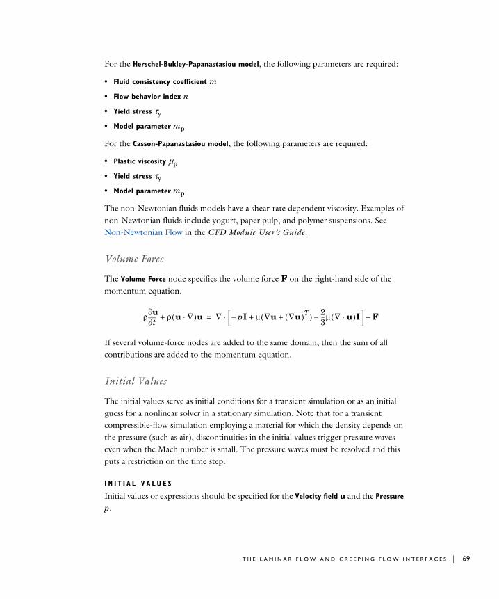
For the Herschel-Bukley-Papanastasiou model, the following parameters are required:

• Fluid consistency coefficient m

• Flow behavior index n



For the Casson-Papanastasiou model, the following parameters are required:

• Plastic viscosity μp



The non-Newtonian fluids models have a shear-rate dependent viscosity. Examples of non-Newtonian fluids include yogurt, paper pulp, and polymer suspensions. See Non-Newtonian Flow in the CFD Module User’s Guide.

Volume Force

The Volume Force node specifies the volume force F on the right-hand side of the momentum equation.

If several volume-force nodes are added to the same domain, then the sum of all contributions are added to the momentum equation.

Initial Values

The initial values serve as initial conditions for a transient simulation or as an initial guess for a nonlinear solver in a stationary simulation. Note that for a transient compressible-flow simulation employing a material for which the density depends on the pressure (such as air), discontinuities in the initial values trigger pressure waves even when the Mach number is small. The pressure waves must be resolved and this puts a restriction on the time step.

I N I T I A L V A L U E S

Initial values or expressions should be specified for the Velocity field u and the Pressure p.

ρt∂

∂u ρ u ∇⋅( )u+ ∇ pI– μ ∇u ∇u( )T+( ) 2

3---μ ∇ u⋅( )I–+⋅ F+=


70 | C H A P T E R

Wall

The Wall node includes a set of boundary conditions describing fluid-flow conditions at stationary, moving, and leaking walls.

B O U N D A R Y C O N D I T I O N

Select a Boundary condition for the wall.

No SlipNo slip is the default boundary condition to model solid walls. A no slip wall is a wall where the fluid velocity relative to the wall velocity is zero. For a stationary wall that means that u = 0.

SlipThe Slip option prescribes a no-penetration condition, u·n=0. It is implicitly assumed that there are no viscous effects at the slip wall and hence, no boundary layer develops. From a modeling point of view, this can be a reasonable approximation if the main effect of the wall is to prevent fluid from leaving the domain.

Electroosmotic VelocityWhen an electric field drives a flow along the boundary, the components for the Electric

field E along with the Electroosmotic mobility μeo should be defined. The Built-in

expression for the Electroosmotic mobility requires values or expressions for the Zeta potential ζ and the Relative permittivity εr.

Slip VelocityIn the microscale range, the flow condition at a boundary is seldom strictly no slip or slip. Instead, the boundary condition is something in between, and there is a Slip

velocity at the boundary. Two phenomena account for this velocity: noncontinuum effects and the flow induced by a thermal gradient along the boundary.

When the Use viscous slip check box is selected, the default Slip length Ls is User defined. Another value or expression may be entered if the default value is not applicable. For Maxwell’s model values or expressions for the Tangential momentum accommodation

coefficient av and the Mean free path λ should be specified. Tangential accommodation coefficients are typically in the range of 0.85 to 1.0 and can be found in G. Kariadakis,

• No Slip

• Slip

• Electroosmotic Velocity

• Slip Velocity

• Leaking Wall

• Navier Slip


A. Beskok, and N. Aluru, Microflows and Nanoflows, Springer Science and Business Media, 2005.

When the Use thermal creep check box is selected, a thermal creep contribution with Thermal slip coefficient σT is activated. Thermal slip coefficients are typically between 0.3 and 1.0 and can be found in G. Kariadakis, A. Beskok, and N. Aluru, Microflows and Nanoflows, Springer Science and Business Media, 2005.

Navier SlipThis boundary condition enforces no-penetration at the wall, , and adds a friction force of the form

where β is a slip length. The boundary condition does not set the tangential velocity component to zero; however, the extrapolated tangential velocity component is 0 at a distance β outside of the wall.

The Slip Length setting is per default set to Factor of minimum element length. The slip length β is then defined as , where is the smallest element side (corresponds to the element size in the wall normal direction for boundary layer elements) and is a user input. Select User defined from Slip Length selection list in order to manually prescribe β.

The Navier Slip boundary condition is suitable for walls adjacent to a fluid-fluid interface or a free surface when solving for laminar flow. Applying this boundary condition, the contact line (fluid-fluid-solid interface) is free to move along the wall.

The Navier Slip option is not available when selecting a turbulence model.

Leaking WallThis boundary condition may be used to simulate a wall where fluid is leaking into or leaving the domain with the velocity u = ul through a perforated wall. The components of the Fluid velocity ul on the leaking wall should be specified.

W A L L M O V E M E N T

This section contains controls to describe the wall movement relative to the lab (or spatial) frame.

The Translational velocity setting controls the translational wall velocity, utr. The list is per default set to Automatic from frame. The physics automatically detects if the spatial frame moves. This can for example happen if an ALE interface is present in the model

u nwall⋅ 0=

Ffrμβ---u–=

β fhhmin= hmin

fh


72 | C H A P T E R

component. If there is no movement utr = 0. If the frame moves, utr becomes equal to the frame movement. utr is accounted for in the actual boundary condition prescribed in the Boundary condition section.

Select Zero (Fixed wall) from Translational velocity selection list to prescribe utr = 0.

Select Manual from Translational velocity selection list in order to manually prescribe Velocity of moving wall, utr. This can for example be used to model an oscillating wall where the magnitude of the oscillations are very small compared to the rest of the model. Specifying translational velocity manually does not automatically cause the associated wall to move. An additional Moving Mesh interface needs to be added to physically track the wall movement in the spatial reference frame.

The Sliding wall option is appropriate if the wall behaves like a conveyor belt; that is, the surface is sliding in its tangential direction. A velocity is prescribed at the wall and the boundary itself does not have to actually move relative to the reference frame.

• For 3D components, values or expressions for the Velocity of sliding wall uw should be specified. If the velocity vector entered is not in the plane of the wall, COMSOL Multiphysics projects it onto the tangential direction. Its magnitude is adjusted to be the same as the magnitude of the vector entered.

• For 2D components, the tangential direction is unambiguously defined by the direction of the boundary. For this reason, the sliding wall boundary condition has different definitions in different space dimensions. A single entry for the Velocity of

the tangentially moving wall Uw should be specified in 2D.

C O N S T R A I N T S E T T I N G S

This section is displayed by clicking the Show button ( ) and selecting Advanced

Physics Options.

Inlet

This condition should be used on boundaries for which there is a net flow into the domain. To obtain a numerically well-posed problem, it is advisable to also consider the Outlet conditions when specifying an Inlet condition. For example, if the pressure is specified at the outlet, the velocity may be specified at the inlet, and vice versa.

• Theory for the Wall Boundary Condition

• The Moving Mesh Interface in the COMSOL Multiphysics Reference Manual


Specifying the velocity vector at both the inlet and the outlet may cause convergence difficulties.


The available Boundary condition options for an inlet are Velocity, Fully developed flow, Mass flow, and Pressure. After selecting a Boundary Condition from the list, a section with the same or a similar name displays underneath. For example, if Velocity is selected, a Velocity section, where further settings are defined, is displayed.

V E L O C I T Y

The Normal inflow velocity is specified as u = −nU0, where n is the boundary normal pointing out of the domain and U0 is the normal inflow speed.

The Velocity field option sets the velocity vector to u = u0. The components of the inlet velocity vector u0 should be defined for this choice.

P R E S S U R E C O N D I T I O N S

This option specifies the normal stress, which in most cases is approximately equal to the pressure. If the reference pressure pref, defined at the physics interface level, is equal to 0, the value of the Pressure p0, at the boundary, is the absolute pressure. Otherwise, p0 is the relative pressure at the boundary.

• The Suppress backflow option adjusts the inlet pressure locally in order to prevent fluid from exiting the domain through the boundary. If you clear the suppress backflow option, the inlet boundary can become an outlet depending on the pressure field in the rest of the domain.

• Flow direction controls in which direction the fluid enters the domain.

- For Normal flow, it prescribes zero tangential velocity component.

- For User defined, an Inflow velocity direction du (dimensionless) should be specified. The magnitude of du does not matter, only the direction. du must point into the domain.

M A S S F L O W

The mass flow at an inlet can be specified by the Mass flow rate, the Pointwise mass flux,

the Standard flow rate, or the Standard flow rate (SCCM).

Mass Flow RateThe Mass flow rate option sets the integrated mass flow across the entire boundary, the Normal mass flow rate to a specific value, m. The mass flow is assumed to be parallel to the boundary normal, and the tangential flow velocity is set to zero.


74 | C H A P T E R

For 2D components, the Channel thickness dbc is used to define the area across which the mass flow occurs. This setting is not applied to the whole model. Line or surface integrals of the mass flow over the boundary evaluated during postprocessing or used in integration coupling operators do not include this scaling automatically. Such results should be appropriately scaled when comparing them with the specified mass flow.

Pointwise Mass FluxThe Pointwise mass flux sets the mass flow parallel to the boundary normal. The tangential flow velocity is set to zero. The mass flux is a model input, which means that COMSOL Multiphysics can take its value from another physics interface when available. When User defined is selected a value or function Mf should be specified for the Mass flux.

Standard Flow RateThe Standard flow rate Qsv sets a standard volumetric flow rate, according to the SEMI standard E12-0303. The mass flow rate is specified as the volumetric flow rate of a gas at standard density — the Mean molar mass Mn divided by a Standard molar volume Vm (that is, the volume of one mole of a perfect gas at standard pressure and standard temperature). The flow occurs across the whole boundary in the direction of the boundary normal and is computed by a surface (3D) or line (2D) integral. The tangential flow velocity is set to zero.

The standard density can be defined directly, or by specifying a standard pressure and temperature, in which case the ideal gas law is assumed. The options in the Standard flow rate defined by list are:

• Standard density, for which the Standard molar volume Vm should be specified.

• Standard pressure and temperature, for which the Standard pressure Pst and the Standard temperature Tst should be defined.

For 2D components, the Channel thickness dbc is used to define the area across which the mass flow occurs. This setting is not applied to the whole model. Line or surface integrals of the mass flow over the boundary evaluated during postprocessing or used in integration coupling operators do not include this scaling automatically. Such results should be appropriately scaled when comparing them with the specified mass flow.

Standard Flow Rate (SCCM)The Standard flow rate (SCCM) boundary condition is equivalent to the Standard flow

rate boundary condition, except that the flow rate is entered directly in SCCMs (standard cubic centimeters per minute) without the requirement to specify units. Here, the dimensionless Number of SCCM units Qsccm should be specified.


F U L L Y D E V E L O P E D F L O W

The Fully developed flow option adds contributions to the inflow boundary, which force the flow towards the solution for a fully developed channel flow. The channel can be thought of as a virtual extrusion of the inlet cross section. The inlet boundary must hence be flat in order for the fully developed flow condition to work properly. In 2D axisymmetric models, the inlet normal must be parallel to the symmetry axis.

Select an option to control the flow rate at the inlet:

• Average velocity, Uav.

• Flow rate, V0. Two-dimensional models also require an Entrance thickness, Dz, which is the out-of-plane thickness of the extruded entrance channel.

• Average pressure, Pav. Observe that Pav is the average pressure on the inflow boundary.

The fully developed flow condition requires any volume force to be approximately aligned with the normal of the inlet boundary. A fully developed flow boundary cannot be adjacent to any Interior Wall feature.



Physics Options.

Outlet

This condition should be used on boundaries for which there is a net outflow from the domain. To obtain a numerically well-posed problem, it is advisable to also consider the Inlet conditions when specifying an Outlet condition. For example, if the velocity is specified at the inlet, the pressure may be specified at the outlet, and vice versa. Specifying the velocity vector at both the inlet and the outlet may cause convergence difficulties. Selecting appropriate outlet conditions for the Navier-Stokes equations is a nontrivial task. Generally, if there is something interesting happening at an outflow boundary, the computational domain should be extended to include this phenomenon.

• Prescribing Inlet and Outlet Conditions

• Normal Stress Boundary Condition


76 | C H A P T E R


The available Boundary condition options for an outlet are Pressure, Fully developed flow, and Velocity.

P R E S S U R E C O N D I T I O N S

This option specifies the normal stress, which in most cases is approximately equal to the pressure. The tangential stress component is set to zero. If the reference pressure pref, defined at the physics interface level, is equal to 0, the value of the Pressure p0, at the boundary, is the absolute pressure. Otherwise, p0 is the relative pressure at the boundary.

• The Normal flow option changes the no tangential stress condition to a no tangential velocity condition. This forces the flow to exit (or enter) the domain perpendicularly to the outlet boundary.

• The Suppress backflow check box is selected by default. This option adjusts the outlet pressure in order to prevent fluid from entering the domain through the boundary.

V E L O C I T Y

See the Inlet node Velocity section for the settings.

F U L L Y D E V E L O P E D F L O W

This boundary condition is applicable when the flow exits the domain into a long pipe or channel, at the end of which a flow profile is fully developed.

The channel can be thought of as a virtual extrusion of the outlet cross section. The outlet boundary must hence be flat in order for the fully developed flow condition to work properly. In 2D axisymmetric models, the outlet normal must be parallel to the symmetry axis.

Select an option to control the flow rate at the outlet:

• Average velocity, Uav.

• Flow rate, V0. Two-dimensional models also require an Entrance thickness, Dz, which is the out-of-plane thickness of the extruded entrance channel.

• Average pressure, Pav. Observe that Pav is the average pressure on the outflow.

The fully developed flow condition requires any volume force to be approximately aligned with the normal of the outlet boundary. A fully developed flow boundary cannot be adjacent to any Interior Wall feature.




Physics Options.

Symmetry

The Symmetry boundary condition prescribes no penetration and vanishing shear stresses. The boundary condition is a combination of a Dirichlet condition and a Neumann condition:

for the compressible and incompressible formulations. The Dirichlet condition takes precedence over the Neumann condition, and the above equations are equivalent to the following equation for both the compressible and incompressible formulations:

B O U N D A R Y S E L E C T I O N

For 2D axial symmetry, a boundary condition does not need to be defined for the symmetry axis at r = 0. The software automatically provides a condition that prescribes ur = 0 and vanishing stresses in the z direction and adds an Axial Symmetry node that implements these conditions on the axial symmetry boundaries only.



Physics Options.

Prescribing Inlet and Outlet Conditions

u n⋅ 0,= pI– μ ∇u ∇u( )T+( ) 23---μ ∇ u⋅( )I–

+ n 0=

u n⋅ 0,= pI– μ ∇u ∇u( )T+( )+( )n 0=

u n⋅ 0,= K K n⋅( )n– 0=

K μ ∇u ∇u( )T+( )n=


78 | C H A P T E R

Open Boundary

The Open Boundary condition describes boundaries in contact with a large volume of fluid. Fluid can both enter and leave the domain on boundaries with this type of condition.

B O U N D A R Y C O N D I T I O N S

The Boundary condition options for open boundaries are Normal stress and No viscous

stress.

Normal StressThe Normal stress f0 condition implicitly imposes .

No Viscous StressThe No Viscous Stress condition specifies vanishing viscous stress on the boundary. This condition does not provide sufficient information to fully specify the flow at the open boundary and must at least be combined with pressure constraints at adjacent points.

The No viscous stress condition prescribes:

for the compressible and the incompressible formulations. This condition can be useful in some situations because it does not impose any constraint on the pressure. A typical example is a model with volume forces that give rise to pressure gradients that are hard to prescribe in advance. To make the model numerically stable, this boundary condition should be combined with a point constraint on the pressure.

Boundary Stress

The Boundary Stress node adds a boundary condition that represents a general class of conditions also known as traction boundary conditions.


The Boundary condition options for the boundary stress are General stress, Normal

stress, and Normal stress, normal flow.

p f0≈

μ ∇u ∇u( )T+( ) 23---μ ∇ u⋅( )I–

n 0=

μ ∇u ∇u( )T+( )n 0=


General StressWhen General stress is selected, the components for the Stress F should be specified. The total stress on the boundary is set equal to the given stress F:

for the compressible and the incompressible formulations.

This boundary condition implicitly sets a constraint on the pressure that for 2D flows is

(3-2)

If ∂un/∂n is small, Equation 3-2 states that p ≈ −n·F.

Normal StressNormal Stress is described for the Open Boundary node.

Normal Stress, Normal FlowFor Normal stress, normal flow, the magnitude of the Normal stress f0 should be specified. The tangential velocity is set to zero on the boundary:

for the compressible and the incompressible formulations.

This boundary condition implicitly sets a constraint on the pressure that for 2D flows is

(3-3)

If ∂un/∂n is small, Equation 3-3 states that p ≈ f0.



Physics Options.

pI– μ ∇u ∇u( )T+( ) 23---μ ∇ u⋅( )I–

+ n F=

pI– μ ∇u ∇u( )T+( )+( )n F=

p 2μ∂un∂n---------- n F⋅–=

nT pI– μ ∇u ∇u( )T+( ) 23---μ ∇ u⋅( )I–

+ n f0,–= t u⋅ 0=

nT pI– μ ∇u ∇u( )T+( )+( )n f0,–= t u⋅ 0=

p 2μ∂un

∂n---------- f0+=


80 | C H A P T E R

If Normal Stress, Normal Flow is selected as the Boundary condition, then to Apply

reaction terms on all dependent variables, the All physics (symmetric) option should be selected. Alternatively, the Individual dependent variables could be selected to restrict the reaction terms as needed.

Periodic Flow Condition

The Periodic Flow Condition splits its selection into a source group and a destination group. Fluid that leaves the domain through one of the destination boundaries enters the domain through the corresponding source boundary. This corresponds to a situation where the geometry is a periodic part of a larger geometry. If the boundaries are not parallel to each other, the velocity vector is automatically transformed.

If the boundaries are curved, the orientation of the source must be specified manually (see Orientation of Source).

No input is required when Compressible flow (Ma<0.3) is selected for Compressibility under the Physical Model section for the physics interface. Typically when a periodic boundary condition is used with a compressible flow, the pressure is the same at both boundaries and the flow is driven by a volume force.

P R E S S U R E D I F F E R E N C E

This section is available when Incompressible flow is selected for Compressibility under the Physical Model section for the physics interface.

A value or expression should be specified for the Pressure difference, psrc − pdst. This pressure difference can, for example, drive the fully developed flow in a channel.

To set up a periodic boundary condition, both boundaries must be selected in the Periodic Flow Condition node. COMSOL Multiphysics automatically assigns one boundary as the source and the other as the destination. To manually set the destination selection, a Destination Selection subnode is available from the context menu (by right-clicking the parent node) or from the Physics toolbar, Attributes menu. All destination sides must be connected.



Physics Options.


O R I E N T A T I O N O F S O U R C E

For information about the Orientation of Source section, see Orientation of Source and Destination in the COMSOL Multiphysics Reference Manual.

Flow Continuity

The Flow Continuity condition is suitable for pairs where the boundaries match; it prescribes that the flow field is continuous across the pair.

A Wall subnode is added by default and it applies to the parts of the pair boundaries where a source boundary lacks a corresponding destination boundary and vice versa. The Wall feature can be overridden by any other boundary condition that applies to exterior boundaries. By right-clicking the Flow Continuity node, additional Fallback feature subnodes can be added.

Pressure Point Constraint

The Pressure Point Constraint condition can be used to specify the pressure level. If it is not possible to specify the pressure level using a boundary condition, the pressure level must be set in some other way, for example, by specifying a fixed pressure at a point.

P R E S S U R E C O N S T R A I N T

The relative pressure value is set by specifying the Pressure p0. Or, if the reference pressure pref defined at the physics interface level is equal to zero, p0 represents the absolute pressure.



Physics Options.

The Apply reaction terms on setting is set per default to Individual dependent variables. All physics (symmetric) cannot be used together with a segregated solver when fluid flow is coupled with Moving Mesh, Level Set, or Phase Field.

Point Mass Source

This feature requires at least one of the following licenses: Batteries & Fuel Cells Module, CFD Module, Chemical Reaction Engineering Module, Corrosion Module,


82 | C H A P T E R

Electrochemistry Module, Electrodeposition Module, Microfluidics Module, Pipe Flow Module, or Subsurface Flow Module.

The Point Mass Source feature models mass flow originating from an infinitely small domain centered around a point

For the Reacting Flow in Porous Media, Diluted Species interface, which is available with the CFD Module, Chemical Reaction Engineering Module, or Batteries & Fuel Cells Module, there are two nodes: one for the fluid flow (Fluid Point Source) and one for the species (Species Point Source).

S O U R C E S T R E N G T H

The source Mass flux, should be specified. A positive value results in mass being ejected from the point into the computational domain. A negative value results in mass being removed from the computational domain.

Point sources located on a boundary or on an edge affect the adjacent computational domains. This has the effect, for example, that a point source located on a symmetry plane has twice the given strength.

Line Mass Source

This feature requires at least one of the following licenses: Batteries & Fuel Cells Module, CFD Module, Chemical Reaction Engineering Module, Corrosion Module, Electrochemistry Module, Electrodeposition Module, Microfluidics Module, Pipe Flow Module, or Subsurface Flow Module.

The Line Mass Source feature models mass flow originating from a tube region with infinitely small radius.

For the Reacting Flow in Porous Media, Diluted Species interface, which is available with the CFD Module, Chemical Reaction Engineering Module, or Batteries & Fuel Cells Module, there are two nodes, one for the fluid flow (Fluid Line Source) and one for the species (Species Line Source).

q·p

Mass Sources for Fluid FlowMass Sources for Fluid Flow in the COMSOL Multiphysics Reference Manual


S E L E C T I O N

The Line Mass Source feature is available for all dimensions, but the applicable selection differs between the dimensions.

S O U R C E S T R E N G T H

The source Mass flux, , should be specified. A positive value results in mass being ejected from the line into the computational domain and a negative value means that mass is removed from the computational domain.

Line sources located on a boundary affect the adjacent computational domains. This, for example, has the effect that a line source located on a symmetry plane has twice the given strength.

Gravity

This feature requires at least one of the following licenses: CFD Module, Heat Transfer Module.

The Gravity global feature is automatically added when Include gravity is selected at the interface level in the Physical Model settings. It defines the gravity forces from the Acceleration of gravity value. When a turbulence model that solves for the turbulent kinetic energy, k, is used, the option Include buoyancy-induced turbulence is available. When selected, the Buoyancy contribution is by default set to Automatic from

multiphysics. Contributions are only obtained from multiphysics couplings that support buoyancy-induced turbulence, such as Nonisothermal Flow. If the Buoyancy

contribution is switched to User defined, an edit field for the Turbulent Schmidt number

appears. See also Theory for Buoyancy-Induced Turbulence in the CFD Module User’s Guide.

MODEL DIMENSION APPLICABLE GEOMETRICAL ENTITY

2D Points

2D Axisymmetry Points not on the axis of symmetry

3D Edges

q· l

Mass Sources for Fluid Flow in the COMSOL Multiphysics Reference Manual


84 | C H A P T E R

A C C E L E R A T I O N O F G R A V I T Y

The Acceleration of gravity (SI unit m/s, default value −gconstez in 2D axial symmetry and 3D and −gconstey in 2D) is used to define the gravity forces. It should be a global quantity.


Th eo r y f o r t h e S i n g l e - Pha s e F l ow I n t e r f a c e s

The theory for the Single-Phase Flow, Laminar Flow interface is described in this section:

• General Single-Phase Flow Theory

• Compressible Flow

• Weakly Compressible Flow

• The Mach Number Limit

• Incompressible Flow

• The Reynolds Number

• Non-Newtonian Flow


• Prescribing Inlet and Outlet Conditions

• Mass Flow

• Fully Developed Flow (Inlet)

• Fully Developed Flow (Outlet)

• No Viscous Stress

• Normal Stress Boundary Condition

• Mass Sources for Fluid Flow

• Numerical Stability — Stabilization Techniques for Fluid Flow

• Solvers for Laminar Flow


• Discontinuous Galerkin Formulation

• Particle Tracing in Fluid Flow

• References for the Single-Phase Flow, Laminar Flow Interfaces

The theory about most boundary conditions is found in Ref. 2.

T H E O R Y F O R T H E S I N G L E - P H A S E F L O W I N T E R F A C E S | 85

86 | C H A P T E R

General Single-Phase Flow Theory

The Single-Phase Fluid Flow interfaces are based on the Navier-Stokes equations, which in their most general form read

(3-4)

(3-5)

(3-6)

where

• ρ is the density (SI unit: kg/m3)

• u is the velocity vector (SI unit: m/s)

• p is pressure (SI unit: Pa)

• τ is the viscous stress tensor (SI unit: Pa)

• F is the volume force vector (SI unit: N/m3)

• Cp is the specific heat capacity at constant pressure (SI unit: J/(kg·K))

• T is the absolute temperature (SI unit: K)

• q is the heat flux vector (SI unit: W/m2)

• Q contains the heat sources (SI unit: W/m3)

• S is the strain-rate tensor:

The operation “:” denotes a contraction between tensors defined by

(3-7)

This is sometimes referred to as the double dot product.

Equation 3-4 is the continuity equation and represents conservation of mass. Equation 3-5 is a vector equation which represents conservation of momentum. Equation 3-6 describes the conservation of energy, formulated in terms of

∂ρ∂t------ ∇ ρu( )⋅+ 0=

ρ∂u∂t------- ρ u ∇⋅( )u+ ∇ pI– τ+[ ]⋅ F+=

ρCp∂T∂t------- u ∇⋅( )T+ ∇ q⋅( )– τ:S T

ρ---- ∂ρ

∂T-------

p

∂p∂t------ u ∇⋅( )p+ – Q+ +=

S 12--- ∇u ∇u( )T+( )=

a:b anmbnm

m

n=


temperature. This is an intuitive formulation that facilitates boundary condition specifications.

To close the equation system, Equation 3-4 through Equation 3-6, constitutive relations are needed. For a Newtonian fluid, which has a linear relationship between stress and strain, Stokes (Ref. 1) deduced the following expression:

(3-8)

The dynamic viscosity, μ (SI unit: Pa·s), for a Newtonian fluid is allowed to depend on the thermodynamic state but not on the velocity field. All gases and many liquids can be considered Newtonian. Examples of non-Newtonian fluids are honey, mud, blood, liquid metals, and most polymer solutions. With the Microfluidics Module, you can model flows of non-Newtonian fluids using the predefined models. The following models which describe the dynamic viscosity for non-Newtonian fluids are avalible: power law, Carreau, Bingham-Papanastasiou, Herschel-Bukley-Papanastasiou, and Casson-Papanastasiou models. The Heat Transfer Module treats all fluids as Newtonian according to Equation 3-8.Other commonly used constitutive relations are Fourier’s law of heat conduction and the ideal gas law.

In theory, the same equations describe both laminar and turbulent flows. In practice, however, the mesh resolution required to simulate turbulence with the Laminar Flow interface makes such an approach impractical.

Many applications describe isothermal flows for which Equation 3-6 is decoupled from Equation 3-4 and Equation 3-5.

2 D A X I S Y M M E T R I C F O R M U L A T I O N S

A 2D axisymmetric formulation of Equation 3-4 and Equation 3-5 requires to be zero. That is, there must be no gradients in the azimuthal direction. A common additional assumption is, however, that . In such cases, the -equation can be removed from Equation 3-5. The resulting system of equations is both easier to converge and computationally less expensive compared to retaining the -equation.

τ 2μS 23---μ ∇ u⋅( )I–=

There are several books where derivations of the Navier-Stokes equations and detailed explanations of concepts such as Newtonian fluids can be found. See, for example, the classical text by Batchelor (Ref. 3) and the more recent work by Panton (Ref. 4).

∂ ∂φ⁄

uφ 0= φ

φ


88 | C H A P T E R

The default 2D axisymmetric formulation of Equation 3-4 and Equation 3-5 therefore assumes that

Compressible Flow

The equations of motion for a single-phase fluid are the continuity equation:

(3-9)

and the momentum equation:

(3-10)

These equations are applicable for incompressible as well as for compressible flow with density and viscosity variations.

Weakly Compressible Flow

The same equations as for Compressible Flow are applied for weakly compressible flow. The only difference is that the density is evaluated at the reference pressure. The density may be a function of other quantities, in particular it may be temperature dependent.

The weakly compressible flow equations are valid for incompressible as well as compressible flow with density variations independent of the pressure.

Provided that the densities dependency pressure is specified through model inputs, the density is automatically evaluated at the reference pressure level.

The Mach Number Limit

An important dimensionless number in fluid dynamics is the Mach number, Ma, defined by

∂ ∂φ⁄ 0=

uφ 0=

∂ρ∂t------ ∇ ρu( )⋅+ 0=

ρ∂u∂t------- ρu ∇u⋅+ ∇p– ∇ μ ∇u ∇u( )T+( ) 2

3---μ ∇ u⋅( )I–

F+⋅+=

Ma ua-------=


where a is the speed of sound. A flow is formally incompressible when Ma = 0. This is theoretically achieved by letting the speed of sound tend to infinity. The Navier-Stokes equations then have the mathematical property that pressure disturbances are instantaneously propagated throughout the entire domain. This results in a parabolic equation system.

The momentum equation, Equation 3-10, is parabolic for unsteady flow and elliptic for steady flow, whereas the continuity equation, Equation 3-9, is hyperbolic for both steady and unsteady flow. The combined system of equations is thus hybrid parabolic-hyperbolic for unsteady flow and hybrid elliptic-hyperbolic for steady flow. An exception occurs when the viscous term in Equation 3-10 becomes vanishingly small, such as at an outflow boundary, in which case the momentum equation becomes locally hyperbolic. The number of boundary conditions to apply on the boundary then depends on the number of characteristics propagating into the computational domain. For the purely hyperbolic system, the number of characteristics propagating from the boundary into the domain changes as the Mach number passes through unity. Hence, the number of boundary conditions required to obtain a numerically well-posed system must also change. The compressible formulation of the laminar and turbulent interfaces uses the same boundary conditions as the incompressible formulation, which implies that the compressible interfaces are not suitable for flows with a Mach number larger than or equal to one.

The practical Mach number limit is lower than one, however. The main reason is that the numerical scheme (stabilization and boundary conditions) of the Laminar Flow interface does not recognize the direction and speed of pressure waves. The fully compressible Navier-Stokes equations do, for example, start to display very sharp gradients already at moderate Mach numbers. But the stabilization for the single-phase flow interface does not necessarily capture these gradients. It is impossible to give an exact limit where the low Mach number regime ends and the moderate Mach number regime begins, but a rule of thumb is that the Mach number effects start to appear at Ma = 0.3. For this reason, the compressible formulation is referred to as Compressible flow (Ma<0.3) in COMSOL Multiphysics.

Incompressible Flow

When the temperature variations in the flow are small, a single-phase fluid can often be assumed incompressible; that is, ρ is constant or nearly constant. This is the case for all liquids under normal conditions and also for gases at low velocities. For constant ρ, Equation 3-9 reduces to


90 | C H A P T E R

(3-11)

and Equation 3-10 becomes

(3-12)

Provided that the densities dependency on temperature and pressure is specified through model inputs, the density is evaluated at the reference pressure level and at the reference temperature. However, if the density is a function of other quantities such as a concentration field, or if the density is specified by a user defined expression, the user has to make sure that the density is defined as constant when the incompressible flow formulation is used.

The Reynolds Number

A fundamental characteristic in analyses of fluid flow is the Reynolds number:

where U denotes a velocity scale, and L denotes a representative length. The Reynolds number represents the ratio between inertial and viscous forces. At low Reynolds numbers, viscous forces dominate and tend to damp out all disturbances, which leads to laminar flow. At high Reynolds numbers, the damping in the system is very low, giving small disturbances the possibility to grow by nonlinear interactions. If the Reynolds number is high enough, the flow field eventually ends up in a chaotic state called turbulence.

Observe that the Reynolds number can have different meanings depending on the length scale and velocity scale. To be able to compare two Reynolds numbers, they must be based on equivalent length and velocity scales.

The Fluid Flow interfaces automatically calculate the local cell Reynolds number Rec = ρ|u|h/(2μ) using the element length h for L and the magnitude of the velocity vector u for the velocity scale U. This Reynolds number is not related to the character of the flow field, but to the stability of the numerical discretization. The risk for numerical oscillations in the solution increases as Rec grows. The cell Reynolds number is a predefined quantity available for visualization and evaluation (typically it is available as: spf.cellRe).

ρ∇ u⋅ 0=

ρt∂

∂u ρ u ∇⋅( )u+ ∇ pI– μ ∇u ∇u( )T+( )+[ ]⋅ F+=

Re ρULμ

------------=


Non-Newtonian Flow

The viscous stress tensor is directly dependent on the strain rate tensor and can be written as:

using the compressible and incompressible formulations. Here denotes the strain-rate tensor defined by:

Its magnitude, the shear rate, is:

where the contraction operator “:” is defined by

For a non-Newtonian fluid, the dynamic viscosity is assumed to be a function of the shear rate:

The Laminar Flow interfaces have five predefined models to prescribe a non-Newtonian viscosity: power law, Carreau, Bingham-Papanastasiou, Herschel-Bukley-Papanastasiou, and Casson-Papanastasiou.

P O W E R L A W

The power law model is an example of a generalized Newtonian model. It prescribes

(3-13)

where m and n are scalars that can be set to arbitrary values. For n > 1, the power law describes a shear thickening (dilatant) fluid. For n < 1, it describes a shear thinning (pseudoplastic) fluid. A value of n equal to one gives the expression for a Newtonian fluid.

τ 2μS 23---μ ∇ u⋅( )I–=

τ 2μS=

S

S 12--- ∇u ∇u( )T+( )=

γ· 2S:S=

a:b anmbnm

m

n=

μ μ γ·( )=

μ mγ· n 1–=


92 | C H A P T E R

Equation 3-13 predicts an infinite viscosity at zero shear rate for n < 1. This is however never the case physically. Instead, most fluids have a constant viscosity for shear rates smaller than 10−2 s−1 (Ref. 17). Since infinite viscosity also makes models using Equation 3-13 difficult to solve, COMSOL Multiphysics implements the power law model as

(3-14)

where is a lower limit for the evaluation of the shear rate magnitude. The default value for is 10−2 s−1, but can be given an arbitrary value or expression using the corresponding text field.

C A R R E A U M O D E L

The Carreau model defines the viscosity in terms of the following four-parameter expression

(3-15)

where λ is a parameter with the unit of time, μ0 is the zero shear rate viscosity, μinf is the infinite shear-rate viscosity, and n is a dimensionless parameter. This expression is able to describe the viscosity for most stationary polymer flows.

B I N G H A M - P A P A N A S T A S I O U

Viscoplastic fluid behavior is characterized by existence of the yield stress τy — a limit which must be exceeded before significant deformation can occur. To model the stress-deformation behavior of viscoplastic materials, different constitutive equations have been propose. The Bingham plastic model is written as

where μp is the plastic viscosity.

To allow computation in both yielded and unyielded region, the Papanastasiou

continuous regularization for the viscosity function is used:

(3-16)

where mp is a scale that controls the exponential growth of stress.

μ mmax γ· γ·min,( )n 1–=

γ·min

γ·min

μ μ∞ μ0 μinf–( ) 1 λγ·( )2+[ ]n 1–( )

2-----------------

+=

μ μpτy

γ·----- τ τy>,+=

μ μpτy

γ·----- 1 mpγ·–( )exp–[ ]+=


H E R S C H E L - B U L K L E Y - P A P A N A S T A S I O U

The Herschel-Bulkley -Papanastasiou model combines the effects of the power law and Bingham behavior:

(3-17)

where m and n are scalars that can be set to arbitrary values. For a value of n equal to one, the Bingham-Papanastasiou model is recovered. This equation is valid in both yielded and unyielded regions. The exponent mp controls the smoothness of the viscosity function.

C A S S O N - P A P A N A S T A S I O U

The Casson-Papanastasiou model combines Casson eqaution with Papanastasiou regularization:

(3-18)

The equation is valid in both yielded and unyielded regions.

Theory for the Wall Boundary Condition

See Wall for the node settings.

S L I P

The Slip condition assumes that there are no viscous effects at the slip wall and hence, no boundary layer develops. From a modeling point of view, this is a reasonable approximation if the important effect of the wall is to prevent fluid from leaving the domain. Mathematically, the constraint can be formulated as:

The no-penetration term takes precedence over the Neumann part of the condition and the above expression is therefore equivalent to

expressing that there is no flow across the boundary and no viscous stress in the tangential direction.

μ mγ· n 1– τy

γ·----- 1 mpγ·–( )exp–[ ]+=

μ μpτy

γ·----- 1 mpγ·–( )exp–[ ]+

2

=

u n⋅ 0,= pI– μ ∇u ∇u( )T+( )+( )n 0=

u n⋅ 0,= K K n⋅( )n– 0=

K μ ∇u ∇u( )T+( )n=


94 | C H A P T E R

For a moving wall with translational velocity utr, u in the above equations is replaced by the relative velocity urel = u−utr.

The boundary condition for ν is .

S L I D I N G W A L L

The sliding wall option is appropriate if the wall behaves like a conveyor belt; that is, the surface is sliding in its tangential direction. The wall does not have to actually move in the coordinate system.

• In 2D, the tangential direction is unambiguously defined by the direction of the boundary, but the situation becomes more complicated in 3D. For this reason, this boundary condition has slightly different definitions in the different space dimensions.

• For 2D and 2D axisymmetric components, the velocity is given as a scalar Uw and the condition prescribes

where t = (ny , −nx) for 2D and t = (nz, −nr) for axial symmetry.

• For 3D components, the velocity is set equal to a given vector uw projected onto the boundary plane:

The normalization makes u have the same magnitude as uw even if uw is not exactly parallel to the wall.

S L I P V E L O C I T Y

In the microscale range, the flow at a boundary is seldom strictly no slip or slip. Instead, the boundary condition is something in between, and there is a slip velocity at the boundary. Two phenomena account for this velocity: violation of the continuum hypothesis for the viscosity and flow induced by a thermal gradient along the boundary.

The following equation relates the viscosity-induced jump in tangential velocity to the tangential shear stress along the boundary:

∇ν n⋅ 0=

u n⋅ 0,= u t⋅ Uw=

uuw n uw⋅( )n–

uw n uw⋅( )n–-------------------------------------------- uw=

Δu 1β---τn t,=


For gaseous fluids, the coefficient β is given by

where μ is the fluid’s dynamic viscosity (SI unit: Pa·s), αv represents the tangential momentum accommodation coefficient (TMAC) (dimensionless), and λ is the molecules’ mean free path (SI unit: m). The tangential accommodation coefficients are typically in the range of 0.85 to 1.0 and can be found in Ref. 16.

A simpler expression for β is

where Ls, the slip length (SI unit: m), is a straight channel measure of the distance from the boundary to the virtual point outside the flow domain where the flow profile extrapolates to zero. This equation holds for both liquids and gases.

Thermal creep results from a temperature gradient along the boundary. The following equation relates the thermally-induced jump in tangential velocity to the tangential gradient of the natural logarithm of the temperature along the boundary:

where σT is the thermal slip coefficient (dimensionless) and ρ is the density of the fluid. The thermal slip coefficients range between 0.3 and 1.0 and can be found in Ref. 16.

Combining the previous relationships results in the following equation:

Relate the tangential shear stress to the viscous boundary force by

where the components of K are the Lagrange multipliers that are used to implement the boundary condition. Similarly, the tangential temperature gradient results from the difference of the gradient and its normal projection:

β μ2 αv–

αv--------------- λ-------------------------=

β μLs------=

Δu σTμρ---∇t Tlog=

u uw t,–Ls

μ------τn t, σT

μρT-------∇tT+=

τn t, K n K⋅( )n–=

∇tT ∇T n ∇T⋅( )n–=


96 | C H A P T E R

Use Viscous SlipWhen viscous slip is used, select Maxwell’s model to calculate Ls using:

Also see Wall for the node settings.

E L E C T R O O S M O T I C V E L O C I T Y

Most solid surfaces acquire a surface charge when brought into contact with an electrolyte. In response to the spontaneously formed surface charge, a charged solution forms close to the liquid-solid interface. This is known as an electric double layer. If an electric field is applied to the fluid, this very narrow layer starts to move along the boundary.

It is possible to model the fluid’s velocity near the boundary using the Helmholtz-Smoluchowski relationship between the electroosmotic velocity u and the applied electric field:

where μeo is the electroosmotic mobility and Et is the fluid electric field tangential to the wall.

Built-in ExpressionUse the Electroosmotic mobility μeo (SI unit: m2/(s·V)) Built-in expression to compute the electroosmotic mobility from:

(3-19)

Here εr is the fluid’s relative permittivity, ε0 the permittivity of free space (SI unit F/m), which is a predefined physical constant, ζ is the fluid’s zeta potential (SI unit: V), and μ the fluid’s dynamic viscosity (Pa·s). Typically μeo≈7×10-8m2/(s·V) and ζ≈100 mV (see H. Bruus, Theoretical Microfluidics, Oxford University Press, 2008). See Wall for the node settings.

Ls2 αv–

αv--------------- λ=

u μeoEt=

μeo εrε0ζμ---–=

Electroosmotic Micromixer: Application Library path Microfluidics_Module/Micromixers/electroosmotic_mixer


Prescribing Inlet and Outlet Conditions

The Navier-Stokes equations can show large variations in mathematical behavior, ranging from almost completely elliptic to almost completely hyperbolic. This has implications when it comes to prescribing admissible boundary conditions. There is also a discrepancy between mathematically valid boundary conditions and practically useful boundary conditions. See Inlet and Outlet for the node settings.

I N L E T C O N D I T I O N S

An inlet requires specification of the velocity components. The most robust way to do this is to prescribe a velocity field using a Velocity condition.

A common alternative to prescribing the complete velocity field is to prescribe a pressure and all but one velocity component. The pressure cannot be specified pointwise because this is mathematically over-constraining. Instead the pressure can be specified via a stress condition:

(3-20)

where ∂un/∂n is the normal derivative of the normal velocity component. Equation 3-20 is prescribed by the Pressure condition in the Inlet and Outlet features and the Normal stress condition in the Open Boundary and Boundary Stress features. Equation 3-20 is mathematically more stringent compared to specifying the pressure pointwise and at the same time cannot guarantee that p obtains the desired value. In practice, p is close to Fn, except for low Reynolds number flows where viscous effects are the only effects that balance the pressure. In addition to Equation 3-20, all but one velocity component must be specified. For low Reynolds numbers, this can be specified by a vanishing tangential stress condition:

which is what the Normal stress condition does. Vanishing tangential stress becomes a less well-posed inlet condition as the Reynolds number increases. The Pressure condition in the Inlet feature therefore requires a flow direction to be prescribed, which provides a well-posed condition independent of Reynolds number.

O U T L E T C O N D I T I O N S

The most common approach is to prescribe a pressure via a normal stress condition on the outlet. This is often accompanied by a vanishing tangential stress condition:

p– 2μun∂n∂---------+ Fn=

μut∂n∂-------- 0=


98 | C H A P T E R

where ∂ut/∂n is the normal derivative of the tangential velocity field. It is also possible to prescribe ut to be zero. The latter option should be used with care since it can have a significant effect on the upstream solution.

The elliptic character of the Navier-Stokes equations mathematically permit specifying a complete velocity field at an outlet. This can, however, be difficult to apply in practice. The reason being that it is hard to prescribe the outlet velocity so that it is consistent with the interior solution at each point. The adjustment to the specified velocity then occurs across an outlet boundary layer. The thickness of this boundary layer depends on the Reynolds number; the higher the Reynolds number, the thinner the boundary layer.

A L T E R N A T I V E F O R M U L A T I O N S

COMSOL provides several specialized boundary conditions that either provide detailed control over the flow at the boundary or that simulate specific devices. In practice they often prescribe a velocity or a pressure, but calculate the prescribed values using for example ODEs.

Mass Flow

The Mass Flow boundary condition constrains the mass flowing into the domain across an inlet boundary. The mass flow can be specified in a number of ways.

P O I N T W I S E M A S S F L U X

The pointwise mass flux sets the velocity at the boundary to:

where mf is the normal mass flux and ρ is the density.

μut∂n∂-------- 0=

Normal Stress Boundary Condition

umfρ-------n–=


M A S S F L O W R A T E

The mass flow rate boundary condition sets the total mass flow through the boundary according to:

where dbc (only present in the 2D Cartesian axis system) is the boundary thickness normal to the fluid-flow domain and m is the total mass flow rate.

In addition to the constraint on the total flow across the boundary, the tangential velocity components are set to zero on the boundary

(3-21)

S T A N D A R D F L O W R A T E

The standard flow rate boundary condition specifies the mass flow as a standard volumetric flow rate. The mass flow through the boundary is set by the equation:

where dbc (only present in the 2D component Cartesian axis system) is the boundary thickness normal to the fluid-flow domain, ρst is the standard density, and Qsv is the standard flow rate. The standard density is defined by one of the following equations:

where Mn is the mean molar mass of the fluid, Vn is the standard molar volume, pst is the standard pressure, R is the universal molar gas constant, and Tst is the standard temperature.

Equation 3-21 or Equation 3-22 is also enforced for compressible and incompressible flow, respectively, ensuring that the normal component of the viscous stress and the tangential component of the velocity are zero at the boundary.

dbcρ u n⋅( ) Sd∂Ω– m=

u n× 0=

dbcρ

ρst------- u n⋅( ) Sd

∂Ω– Qsv=

ρstMn

Vn--------=

ρstpstMnRTst-----------------=


100 | C H A P T E

Fully Developed Flow (Inlet)

The Fully Developed Flow boundary condition can be understood from the following figure:

The flow to the domain Ω is assumed to enter through a straight channel of length L. The channel is a virtual extrusion of the inlet cross section and a pressure constant pressure Pinl is applied on the inlet of the virtual channel.

The Fully Developed Flow boundary condition prescribes that the tangential flow component on the boundary is zero:

The momentum equation for a fully developed flow in the virtual extrusion of the inlet cross section can then be projected onto the inlet boundary with the following weak equation as the result:

The exact value of L is somewhat arbitrary as long as it is not too high or too low. L is therefore set to ten times the inlet edge length in 2D and to ten times the square root of the inlet area in 2D axisymmetry and in 3D.

The fact that the velocity profile is not prescribed, but rather the solution of a projected weak contribution, means that the actual velocity profile that is obtained on the inlet can deviate from the analytical fully developed flow profile (in cases such an analytical solution exists) if required by the solution inside the computational domain, Ω. This is most notably if the flow is strongly curved just downstream of the inlet. This can for example be the case if an object is positioned just downstream of the inlet or if the adjacent boundaries are not orthogonal to the inlet. The analytical solution can in these cases be recovered by including a little bit of the inlet channel in the computational domain.

The inlet pressure, Pinl, must be solved for and the its equation is a discrete algebraic equation (DAE) for Pinl. When, for example, the average velocity is specified, the DAE reads

L

Ωpinl

u u n⋅( )n– 0=

μ– ut∇ ut∇( )T+( ) p+( ) uLt∇ Pinl n u⋅( )–

R 3 : S I N G L E - P H A S E F L O W I N T E R F A C E S

where <⋅> denotes the average over the inlet. Since the equation for Pinl is a DAE (the equation for Pinl does not contain Pinl), it must be solved coupled to Navier-Stokes and it must be treated by a Vanka pre- and post-smoother if iterative solvers are employed.

The boundary conditions for the virtual inlet channel are inherited from the boundaries adjacent to the inlet channel. Virtual boundaries adjacent to walls (except slip walls) are treated as no-slip walls. Virtual boundaries adjacent to any other type of boundary are treated as slip-walls (or equivalently as symmetry boundaries). So in the figure above, if the lower boundary of Ω is a no-slip wall and the top boundary is a symmetry boundary, the lower boundary of the virtually extruded channel becomes a no-slip wall and the upper boundary a symmetry boundary.

Algebraic turbulence models need to additional equations or constraints. For all other turbulence models, their weak equations in the virtual inlet channel are projected onto the inlet of the computational domain. The projections are regularized to prevent the production to fall to zero, so the solutions of the projects can show slight deviation from the correct solutions close to no-slip walls.

Fully Developed Flow (Outlet)

The Fully Developed Flow boundary condition can be understood from the following figure:

The flow to the domain Ω is assumed to enter through a straight channel of length L. The channel is a virtual extrusion of the inlet cross section and a pressure constant pressure Pexit is applied on the inlet of the virtual channel.

The Fully Developed Flow boundary condition prescribes that the tangential flow component on the boundary is zero:

u n⋅ Uav+( )Pinl

Ω pexit

L

u u n⋅( )n– 0=


102 | C H A P T E

The momentum equation for a fully developed flow in the virtual extrusion of the inlet cross section can then be projected onto the inlet boundary with the following weak equation as the result:

The exact value of L is somewhat arbitrary as long as it is not too high or too low. L is therefore set to ten times the inlet edge length in 2D and to ten times the square root of the inlet area in 2D axisymmetry and in 3D.

The fact that the velocity profile is not prescribed, but rather the solution of a projected weak contribution, means that the actual velocity profile that is obtained on the outlett can deviate from the analytical fully developed flow profile (in cases such an analytical solution exists) if required by the solution inside the computational domain, Ω. The inlet pressure, Pexit, must be solved for and the its equation is a discrete algebraic equation (DAE) for Pexit. When, for example, the average velocity is specified, the DAE reads

where <⋅> denotes the average over the inlet. Since the equation for Pext is a DAE, it must be solved coupled to Navier-Stokes and it must be treated by a Vanka pre- and post-smoother if iterative solvers are employed.

The boundary conditions for the virtual outlet channel are inherited from the boundaries adjacent to the outlet channel. Virtual boundaries adjacent to walls (except slip walls) are treated as no-slip walls. Virtual boundaries adjacent to any other type of boundary are treated as slip-walls (or equivalently as symmetry boundaries).

No Viscous Stress

For this module, and in addition to the Pressure, No Viscous Stress boundary condition, the viscous stress condition sets the viscous stress to zero:

using the compressible/weakly compressible and the incompressible formulation, respectively.

μ– ut∇ ut∇( )T+( ) p+( ) uLt∇ Pexit n u⋅( )–

u n⋅ Uav+( )Pexit

μ ∇u ∇u( )T+( ) 23---μ ∇ u⋅( )I–

n 0=

μ ∇u ∇u( )T+( )( )n 0=


The condition is not a sufficient outlet condition since it lacks information about the outlet pressure. It must hence be combined with pressure point constraints on one or several points or lines surrounding the outlet.

This boundary condition is numerically the least stable outlet condition, but can still be beneficial if the outlet pressure is nonconstant due to, for example, a nonlinear volume force.

Normal Stress Boundary Condition

The total stress on the boundary is set equal to a stress vector of magnitude f0, oriented in the negative normal direction:


This implies that the total stress in the tangential direction is zero. This boundary condition implicitly sets a constraint on the pressure which for 2D flows is

(3-22)

If ∂un/∂n is small, Equation 3-22 states that p ≈ f0.

The Normal Stress condition is the mathematically correct version of the Pressure Conditions condition (Ref. 4), but it is numerically less stable.

Pressure Boundary Condition

For single-phase flow, a mathematically correct natural boundary condition for outlets is

(3-23)

(3-24)

pI– μ ∇u ∇u( )T+( ) 23---μ ∇ u⋅( )I–

+ n f0n–=

pI– μ ∇u ∇u( )T+( )+( )n f0n–=

p 2μ∂un∂n---------- f0+=

pI– μ ∇u ∇u( )T+( ) 23---μ ∇ u⋅( )I–+

n p0n–=

pI– μ ∇u ∇u( )T+( )+( )n p0n–=


104 | C H A P T E


This is a normal stress condition together with a no-tangential-stress condition. When μ > 0, Equation 3-23 or Equation 3-24 can be supplemented with a tangential velocity condition

u⋅t = 0 (3-25)

If so, the no-tangential-stress condition is overridden. An issue with Equation 3-23 or Equation 3-24 is that it does not strongly enforce unidirectional flow on the boundary. If the prescribed pressure on an outlet is too high, parts of the outlet can actually have inflow. This is not as much of an issue for the Navier-Stokes equations as it is an issue for scalar transport equations solved along with the Navier-Stokes equations. Hence, when applying the Pressure boundary condition at an outlet or inlet you can further constrain the flow. With the Suppress backflow option

, (3-26)

the normal stress is adjusted to keep

(3-27)

Equation 3-26 effectively means that the prescribed pressure is p0 if u⋅n ≥ 0, but smaller at locations where u⋅n < 0. This means that Equation 3-26 does not completely prevent backflow, but the backflow is substantially reduced. Backflow is suppressed also when external forces are acting on the fluid, provided the magnitude of these forces are of the same order as the dynamic pressure at the outlet.

A pressure condition can also be applied at an inlet. In this case, either the normal stress is prescribed

(3-28)

pI– μ ∇u ∇u( )T+( ) 23---μ ∇ u⋅( )I–+

n p0n–=

pI– μ ∇u ∇u( )T+( )+( )n p0n–=

p0 p0≤

u n⋅ 0≥

nT pI– μ ∇u ∇u( )T+( ) 23---μ ∇ u⋅( )I–+

n p0–=

nT pI– μ ∇u ∇u( )T+( )+( )n p0–=

p0 p0≥


together with the tangential condition in Equation 3-25, or, a general flow direction is prescribed.

(3-29)

The “>” option is used with suppress backflow to have or .

See Inlet, Outlet, Open Boundary, and No Viscous Stress for the individual node settings. Note that some modules have additional theory sections describing options available with that module.

Mass Sources for Fluid Flow

There are two types of mass sources in a Single-Phase Flow interface: point sources and line sources.

P O I N T S O U R C E

A point source is theoretically formed by taking a mass injection/ejection, (SI unit: kg/(m3·s)), in a small volume δV and then letting the size of the volume tend to zero while keeping the total mass flux constant. Given a point source strength, (SI unit: kg/s), this can be expressed as

(3-30)

An alternative way to form a point source/sink is to assume that mass is injected/extracted through the surface of a small object. Letting the object surface

ruT pI– μ ∇u ∇u( )T+( ) 2

3---μ ∇ u⋅( )I–+

n p0 ru n⋅( )–=

ruT pI– μ ∇u ∇u( )T+( )+( )n p0 ru n⋅( )–=

p0 p0≥

u u ru⋅( )ru 0 rududu-------------=,=–

u n 0≤⋅ u ru 0≥⋅

These features require at least one of the following licenses: Batteries & Fuel Cells Module, CFD Module, Chemical Reaction Engineering Module, Corrosion Module, Electrochemistry Module, Electrodeposition Module, Microfluidics Module, Pipe Flow Module, or Subsurface Flow Module.

Q·

q·p

δV 0→lim Q

·

δV q·p=


106 | C H A P T E

area tend to zero while keeping the mass flux constant, results in the same point source. For this alternative approach, effects resulting from the physical object volume, such as drag and fluid displacement, need to be neglected.

The weak contribution

is added to a point in the geometry. As can be seen from Equation 3-30, must tend to plus or minus infinity as δV tends to zero. This means that in theory the pressure also tends to plus or minus infinity.

Observe that “point” refers to the physical representation of the source. A point source can therefore only be added to points in 3D components and to points on the symmetry axis in 2D axisymmetry components. Other geometrical points in 2D components represent physical lines.

The finite element representation of Equation 3-30 corresponds to a finite pressure in a point with the effect of the point source spread out over a region around the point. The size of the region depends on the mesh and on the strength of the source. A finer mesh gives a smaller affected region, but also a more extreme pressure value. It is important not to mesh too finely around a point source since the resulting pressure can result in unphysical values for the density, for example. It can also have a negative effect on the condition number for the equation system.

L I N E S O U R C E

A line source can theoretically be formed by assuming a source of strength (SI unit: kg/(m3·s)), located within a tube with cross-sectional area δS and then letting δS tend to zero, while keeping the total mass flux per unit length constant. Given a line source strength, (SI unit: kg/(m·s)), this can be expressed as

(3-31)

As in the point source case, an alternative approach is to assume that mass is injected/extracted through the surface of a small object. This results in the same mass source, but requires that effects on the fluid resulting from the physical object volume are neglected.


q·ptest p( )

Q·

Q·

q· l

δS 0→lim Q

·

δS q· l=

q· ltest p( )


is added to lines in 3D or to points in 2D (which represent cut-through views of lines). Line sources can also be added to the axisymmetry line in 2D axisymmetry components. It cannot, however, be added to geometrical lines in 2D because they represent physical planes.

As with a point source, it is important not to mesh too finely around the line source.

Numerical Stability — Stabilization Techniques for Fluid Flow

The momentum equation (Equation 3-10 or Equation 3-12) is a (nonlinear) convection-diffusion equation. Such equations can easily become unstable if discretized using the Galerkin finite element method. Stabilized finite element methods are usually necessary in order to obtain physical solutions. The stabilization settings are found in the main Fluid Flow interface features. To display this section, click the Show button ( ) and select Stabilization.

There are three types of stabilization methods available for Navier-Stokes — streamline diffusion, crosswind diffusion, and isotropic diffusion. Streamline diffusion and crosswind diffusion are consistent stabilization methods, whereas isotropic diffusion is an inconsistent stabilization method.

For optimal functionality, the exact weak formulations of and constants in the streamline diffusion and crosswind diffusion methods depend on the order of the shape functions (basis functions) for the elements. The values of constants in the streamline diffusion and crosswind diffusion methods follow Ref. 5 and Ref. 6.

For feature node information, see Line Mass Source and Point Mass Source in the COMSOL Multiphysics Reference Manual.

For the Reacting Flow in Porous Media, Diluted Species interface, which is available with the CFD Module, Chemical Reaction Engineering Module, or Batteries & Fuel Cells Module, these shared physics nodes are renamed as follows:

• The Line Mass Source node is available as two nodes, one for the fluid flow (Fluid Line Source) and one for the species (Species Line Source).

• The Point Mass Source node is available as two nodes, one for the fluid flow (Fluid Point Source) and one for the species (Species Point Source).


108 | C H A P T E

S T R E A M L I N E D I F F U S I O N

For strongly coupled systems of equations, the streamline diffusion method must be applied to the system as a whole rather than to each equation separately. These ideas were first explored by Hughes and Mallet (Ref. 7) and were later extended to Galerkin least-squares (GLS) applied to the Navier-Stokes equations (Ref. 8). This is the streamline diffusion formulation that COMSOL Multiphysics supports. The time-scale tensor is the diagonal tensor presented in Ref. 9.

The time-scale tensors for time-dependent problems should in theory depend on a time-scale that many references just set to the time-step taken by the time-solver, Δt (see for example Ref. 8 and Ref. 9). This simple approach doesn’t however necessarily reflect on the actual time-scales in the physics. A typical example is reacting flows where the time-step is often guided by fast reactions, while the flow develops relatively slowly. COMSOL Multiphysics therefore replaces Δt2 in the time scale tensor with measures of type which are calculated from projections of weak expressions in a fashion similar to those in Ref. 10. Streamline diffusion is active by default because it is necessary when convection is dominating the flow.

The governing equations for incompressible flow are subject to the Babuška-Brezzi condition, which states that the shape functions (basis functions) for pressure must be of lower order than the shape functions for velocity. If the incompressible Navier-Stokes equations are stabilized by streamline diffusion, it is possible to use equal-order interpolation. Hence, streamline diffusion is necessary when using first-order elements for both velocity and pressure. This applies also if the model is solved using geometric multigrid (either as a solver or as a preconditioner) and at least one multigrid hierarchy level uses linear Lagrange elements.

C R O S S W I N D D I F F U S I O N

Crosswind diffusion can also be formulated for systems of equations, and when applied to the Navier-Stokes equations it becomes a shock-capturing operator. COMSOL Multiphysics supports the formulation in Ref. 8 with a shock-capturing viscosity of the Hughes-Mallet type Ref. 7.

Incompressible flows do not contain shock waves, but crosswind diffusion is still useful for introducing extra diffusion in sharp boundary layers and shear layers that otherwise would require a very fine mesh to resolve.

Crosswind diffusion is active by default as it makes it easier to obtain a solution even if the problem is fully resolved by the mesh. Crosswind diffusion also enables the iterative solvers to use inexpensive presmoothers. If crosswind diffusion is deactivated, more expensive preconditioners must be used instead.

1 Δ t( )2⁄( ) 1–


I S O T R O P I C D I F F U S I O N

Isotropic diffusion adds diffusion to the Navier-Stokes equations. Isotropic diffusion significantly reduces the accuracy of the solution but does a very good job at reducing oscillations. The stability of the continuity equation is not improved.

Solvers for Laminar Flow

The Navier-Stokes equations constitute a nonlinear equation system. A nonlinear solver must hence be applied to solve the problem. The nonlinear solver iterates to reach the final solution. In each iteration, a linearized version of the nonlinear system is solved using a linear solver. In the time-dependent case, a time marching method must also be applied. The default suggestions for each of these solver elements are discussed below.

N O N L I N E A R S O L V E R

The nonlinear solver method depends on if the model solves a stationary or a time-dependent problem.

Stationary SolverIn the stationary case, a fully coupled, damped Newton method is applied. The initial damping factor is low since a full Newton step can be harmful unless the initial values are close to the final solution. The nonlinear solver algorithm automatically regulates the damping factor in order to reach a converged solution.

For advanced models, the automatically damped Newton method might not be robust enough. A pseudo time-stepping algorithm can then be invoked. See Pseudo Time Stepping for Laminar Flow Models.

Time-Dependent SolverIn the time-dependent case, the initial guess for each time step is (loosely speaking) the previous time step, which is a very good initial value for the nonlinear solver. The automatic damping algorithm is then not necessary. The damping factor in the Newton method is instead set to a constant value slightly smaller than one. Also, for the same reason, it suffices to update the Jacobian once per time-step.

Numerical Stabilization and Iterative in the COMSOL Multiphysics Reference Manual


110 | C H A P T E

It is seldom worth the extra computational cost to update the Jacobian more than once per time step. For most models it is more efficient to restrict the maximum time step or possibly lower the damping factor in the Newton method.

L I N E A R S O L V E R

The linearized Navier-Stokes equation system has saddle point character, unless the density depends on the pressure. This means that the Jacobian matrix has zeros on the diagonal. Even when the density depends on the pressure, the equation system effectively shares many numerical properties with a saddle point system.

For small 2D and 3D models, the default solver suggestion is a direct solver. Direct solvers can handle most nonsingular systems and are very robust and also very fast for small models. Unfortunately, they become slow for large models and their memory requirement scales as somewhere between N1.5and N2, where N is the number of degrees of freedom in the model. The default suggestion for large 2D and 3D models is therefore the iterative GMRES solver. The memory requirement for an iterative solver optimally scales as N.

GMRES is accelerated by a multigrid method, per default the Smoothed Aggregation Algebraic Mutligrid (SAAMG) method. The cost of SAAMG is typically very low compared to the number of GMRES iterations necessary if no multigrid method is used. As the name implies, SAAMG builds its coarser meshes algebraically, so the application requires no additional meshes in order to employ SAAMG. In contrast, Geometric Multigrid (GMG) requires actual meshes. If a sufficient number of multigrid levels can be constructed, GMG is often faster than SAAMG. GMG is also superior for cluster computations and for shared memory computations with many cores. When the default linear solver is GMRES, an optional, but deactivated, linear solver node is available where GMRES is accelerated by GMG.

Multigrid methods need smoothers, but the saddle point character of the linear system restricts the number of applicable smoothers. The choices are further restricted by the anisotropic meshes frequently encountered in fluid-flow problems. The efficiency of the smoothers is highly dependent on the numerical stabilization. Iterative solvers perform at their best when both Streamline Diffusion and Crosswind Diffusion are active.

The default smoother for P1+P1 elements is SCGS. This is an efficient and robust smoother specially designed to solve saddle point systems on meshes that contain anisotropic elements. The SCGS smoother works well even without crosswind diffusion. SCGS can sometimes work for higher-order elements, especially if Method in the SCGS settings is set to Mesh element lines. But there is no guarantee for this, so the


default smoother for higher order elements is an SOR Line smoother. SOR Line handles mesh anisotropy but does not formally address the saddle point character. It does, however, function in practice provided that streamline diffusion and crosswind diffusion are both active.

A different kind of saddle point character can arise if the equation system contains ODE variables. Some advanced boundary conditions can add equations with such variables. These variables must be treated with the Vanka algorithm. SCGS includes an option to invoke Vanka. Models with higher-order elements must apply SCGS or use the Vanka smoother. The latter is the default suggestion for higher-order elements, but it does not work optimally for anisotropic meshes.

T I M E - D E P E N D E N T S O L V E R S

The default time-dependent solver for Navier-Stokes is the BDF method with maximum order set to two. Higher BDF orders are not stable for transport problems in general nor for Navier-Stokes in particular.

BDF methods have been used for a long time and are known for their stability. However, they can have severe damping effects, especially the lower-order methods. Hence, if robustness is not an issue, a model can benefit from using the generalized-α method instead. Generalized-α is a solver which has properties similar to those of the second-order BDF solver but it is much less diffusive.

Both BDF and generalized-α are per default set to automatically adjust the time step. While this works well for many models, extra efficiency and accuracy can often be gained by specifying a maximum time step. It is also often beneficial to specify an initial time step to make the solver progress smoothly in the beginning of the time series.

Pseudo Time Stepping for Laminar Flow Models

A stationary formulation has per definition no time derivatives and Equation 3-12 reduces to:

(3-32)


• Time-Dependent Solver

• Multigrid, Direct, Iterative, SCGS, SOR Line, and Vanka

• Stationary Solver

ρ u ∇⋅( )u ∇ pI– μ ∇u ∇u( )T+( )+[ ]⋅ F+=


112 | C H A P T E

Solving Equation 3-32 requires a starting guess that is close enough to the final solution. If no such guess is at hand, the fully transient problem can be solved instead. This is, however, a rather costly approach in terms of computational time. An intermediate approach is to add a fictitious time derivative to Equation 3-32:

where is a pseudo time step. Since u−nojac(u) is always zero, this term does not affect the final solution. It does, however, affect the discrete equation system and effectively transforms a nonlinear iteration into a step of size of a time-dependent solver.

Pseudo time stepping is not active per default. The pseudo time step can be chosen individually for each element based on the local CFL number:

where h is the mesh cell size. A small CFL number means a small time step. It is practical to start with a small CFL number and gradually increase it as the solution approaches steady state.

If the automatic expression for CFLloc is set to the built-in variable CFLCMP, then the automatic setting suggests a PID regulator for the pseudo time step in the default solver. The PID regulator starts with a small CFL number and increases CFLloc as the solution comes closer to convergence.

The default manual expression is

(3-33)

The variable niterCMP is the nonlinear iteration number. It is equal to one for the first nonlinear iteration. CFLloc starts at 1.3 and increases by 30% each iteration until it reaches . It remains there until iteration number 20 at which it starts to increase until it reaches approximately 106. A final increase after iteration number 40

ρu nojac u( )–

Δ t--------------------------------- ρ+ u ∇⋅( )u ∇ pI– μ ∇u ∇u( )T

+( )+[ ]⋅ F+=

Δ t

Δ t

Δ t

Δ t CFLlochu-------=

1.3min niterCMP 9,( ) +

if niterCMP 20> 9 1.3min niterCMP 20– 9,( )⋅ 0, ,( ) +

if niterCMP 40> 90 1.3min niterCMP 40– 9,( )⋅ 0, ,( )

1.39 10.6≈


then takes it to 1060. Equation 3-33 can, for some advanced flows, increase CFLloc too slowly or too quickly. CFLloc can then be tuned for the specific application.

Discontinuous Galerkin Formulation

Some boundary conditions are implemented using a discontinuous Galerkin formulation. These boundary conditions include

• Wall — Slip, sliding walls, and moving walls (that is, walls with nonzero translational velocity).


• Flow Continuity

The formulation used in the Fluid Flow interfaces in COMSOL Multiphysics is the Symmetric Interior Penalty Galerkin method (SIPG). The SIPG method can be regarded to satisfy the boundary conditions in an integral sense rather than pointwise. More information on SIPG can be found in Ref. 14.

In particular, the SIPG formulation includes a penalty parameter that must be large enough for the formulation to be coercive. The higher the value, the better the boundary condition is fulfilled, but a too high value results in an ill-conditioned equation system. The penalty parameter in COMSOL Multiphysics is implemented according to Ref. 15.

Particle Tracing in Fluid Flow

The Particle Tracing Module is available to assist with these types of modeling problems.

It is possible to model particle tracing with COMSOL Multiphysics provided that the impact of the particles on the flow field is negligible. First compute the flow field, and then, as an analysis step, calculate the motion of the particles. The motion of a particle is defined by Newton’s second law

For details about the CFL regulator, see Pseudo Time Stepping in the COMSOL Multiphysics Reference Manual.

mt2

2

dd x F t x

tddx, ,

=


114 | C H A P T E

where x is the position of the particle, m the particle mass, and F is the sum of all forces acting on the particle. Examples of forces acting on a particle in a fluid are the drag force, the buoyancy force, and the gravity force. The drag force represents the force that a fluid exerts on a particle due to a difference in velocity between the fluid and the particle. It includes the viscous drag, the added mass, and the Basset history term. Several empirical expressions have been suggested for the drag force. One of those is the one proposed by Khan and Richardson (Ref. 12). That expression is valid for spherical particles for a wide range of particle Reynolds numbers. The particle Reynolds number is defined as

where u is the velocity of the fluid, up the particle velocity, r the particle radius, ρ the fluid density, and μ the dynamic viscosity of the fluid. The empirical expression for the drag force according to Khan and Richardson is

References for the Single-Phase Flow, Laminar Flow Interfaces

1. G.G. Stokes, Trans. Camb. Phil. Soc., 8, pp. 287–305, 1845

2. P.M. Gresho and R.L. Sani, Incompressible Flow and the Finite Element Method, Volume 2: Isothermal Laminar Flow, John Wiley & Sons, 2000.

3. G.K. Batchelor, An Introduction To Fluid Dynamics, Cambridge University Press, 1967.

4. R.L. Panton, Incompressible Flow, 2nd ed., John Wiley & Sons, 1996.

5. I. Harari and T.J.R. Hughes, “What are C and h? Inequalities for the Analysis and Design of Finite Element Methods”, Comp. Meth. Appl. Mech. Engrg, vol. 97, pp. 157–192, 1992.

Repu up– 2rρ

μ------------------------------=

F πr2 ρ u up– u up–( ) 1.84Rep-0.31 0.293Rep

0.06+[ ]3.45

=

The model Flow Past a Cylinder (Application Library path COMSOL_Multiphysics/Fluid_Dynamics/cylinder_flow) demonstrates how to add and set up particle tracing in a plot group using the Particle Tracing

with Mass node. It uses the predefined Khan-Richardson model for the drag force and neglects gravity and buoyancy forces.


6. Y. Bazilevs, V.M. Calo, T.E. Tezduyar, and T.J.R. Hughes, “YZβ Discontinuity Capturing for Advection-dominated Processes with Application to Arterial Drug Delivery”, Int.J.Num. Meth. Fluids, vol. 54, pp. 593–608, 2007.

7. T.J.R. Hughes and M. Mallet, “A New Finite Element Formulation for Computational Fluid Dynamics: III. The Generalized Streamline Operator for Multidimensional Advective-Diffusive System”, Comp. Meth. Appl. Mech. Engrg, vol. 58, pp. 305–328, 1986.

8. G. Hauke and T.J.R. Hughes, “A Unified Approach to Compressible and Incompressible Flows”, Comp. Meth. Appl. Mech. Engrg, vol. 113, pp. 389–395, 1994.

9. G. Hauke, “Simple Stabilizing Matrices for the Computation of Compressible Flows in Primitive Variables”, Comp. Meth. Appl. Mech. Engrg, vol. 190, pp. 6881–6893, 2001.

10. M.-C. Hsu, Y. Bazilevs, V.M. Cali, T.E. Tezduyar, and T.J.R. Hughes, “Improving stability of stabilized and multiscale formulations in flow simulations at small time steps”, Comp. Meth. Appl. Mech. Engrg, vol. 199, pp. 828–840, 2010.

11. D.J. Tritton, Physical Fluid Dynamics, 2nd ed., Oxford University Press, 1988.

12. J.M. Coulson and J.F. Richardson, “Particle Technology and Separation Processes”, Chemical Engineering, Volume 2, Butterworth-Heinemann, 2002.

13. J.L. Guermond, P. Minev, and J. Shen, “An overview of projection methods for incompressible flows”, Comp. Meth. Appl. Mech. Engrg, vol. 195, pp. 6011–6045, 2006.

14. B. Rivière, Discontinuous Galerkin Methods for Solving Elliptic and Parabolic Equations, SIAM, 2008.

15. Y. Epshteyn and B. Rivière, “Estimation of penalty parameters for symmetric interior penalty Galerkin methods”, J. Computational and Applied Mathematics, vol. 206, pp. 843–872, 2007.


17. R.P. Chhabra and J.F. Richardson, Non-Newtonian Flow and Applied Rheology, 2nd ed., Elsevier, 2008.


116 | C H A P T E

4

M u l t i p h a s e F l o w , T w o - P h a s e F l o wI n t e r f a c e s

There are several Fluid Flow interfaces available with the Microfluidics Module. These are found under the Fluid Flow>Multiphase Flow branch ( ) when adding a physics interface. See Modeling Microfluidic Fluid Flows to help select the physics interface to use.

In this chapter:

• The Laminar Two-Phase Flow, Level Set and Laminar Two-Phase Flow, Phase Field Interfaces

• The Laminar Three-Phase Flow, Phase Field Interface

• The Laminar Two-Phase Flow, Moving Mesh Interface

• Theory for the Level Set and Phase Field Interfaces

• Theory for the Three-Phase Flow, Phase Field Interface

• Theory for the Two-Phase Flow, Moving Mesh Interface

| 117

118 | C H A P T E

Th e L am i n a r Two -Pha s e F l ow , L e v e l S e t and L am i n a r Two -Pha s e F l ow , Pha s e F i e l d I n t e r f a c e s

This section includes the following topics:

• The Laminar Two-Phase Flow, Level Set Interface

• T he Two-Phase Flow, Level Set Coupling Feature

• The Wetted Wall Coupling Feature

• The Laminar Two-Phase Flow, Phase Field Interface

• The Two-Phase Flow, Phase Field Coupling Feature

• Domain, Boundary, Point, and Pair Nodes for the Laminar Flow, Two-Phase, Level Set and Phase Field Interfaces

The Laminar Two-Phase Flow, Level Set Interface

The Laminar Two-Phase Flow, Level Set interface ( ) found under the Multiphase

Flow>Two-Phase Flow, Level Set branch ( ), is a multiphysics interface designed to track the interface between two immiscible fluids. The flow is assumed to be laminar, that is, to be of low to moderate Reynolds number. The fluids can be incompressible or compressible.

When adding the Laminar Two-Phase Flow, Level Set multiphysics interface, a Laminar

Flow and a Level Set interface are added to the Model Builder. In addition, a multiphysics coupling feature, T he Two-Phase Flow, Level Set Coupling Feature, is added automatically under the Multiphysics node. Another multiphysics coupling feature, The Wetted Wall Coupling Feature, can be added when needed.

Simulations using the Laminar Two-Phase Flow, Level Set interface are always time-dependent since the position of an interface is almost always dependent of its history.

Mathematics, Moving Interfaces

R 4 : M U L T I P H A S E F L O W , T W O - P H A S E F L O W I N T E R F A C E S

T H E L A M

I N T E R F A C E P R O P E R T I E S

DiscretizationBy default the fluid flow discretization is set to P1+P1, and the level set discretization is set to Linear. This combination provides exact conservation of the integral of the level set variable when using the nonconservative form of the level set equation.

T he Two-Phase Flow, Level Set Coupling Feature

The Laminar Two-Phase Flow, Level Set, ( ) and Turbulent Two-Phase Flow, Level Set,

( ) interfaces contain a multiphysics coupling feature, Two-Phase Flow, Level Set, which is added automatically.

The Two-Phase Flow, Level Set multiphysics coupling feature defines the density and dynamic viscosity of the fluid used in the Laminar Flow interface, and it defines the surface tension on the interface in form of a volume force used in the momentum equation. It also enables the Level Set interface to use the velocity field calculated from the Laminar Flowinterface to transport the interface.

S E T T I N G S

The Label is the default multiphysics coupling feature name.

The Name is used primarily as a scope prefix for variables defined by the coupling node. Refer to such variables in expressions using the pattern <name>.<variable_name>. In order to distinguish between variables belonging to different coupling nodes or physics interfaces, the name string must be unique. Only letters, numbers, and underscores (_) are permitted in the Name field. The first character must be a letter.

The default Name (for the first multiphysics coupling feature Two-Phase Flow, Level Set

in the model) is tpf1.

D O M A I N S E L E C T I O N

When nodes are added from the context menu, you can select All domains (the default) or select Manual from the Selection list to choose specific domains.



I N A R T W O - P H A S E F L O W , L E V E L S E T A N D L A M I N A R T W O - P H A S E F L O W , P H A S E F I E L D I N T E R F A C E S | 119

120 | C H A P T E

C O U P L E D I N T E R F A C E S

This section controls which individual interfaces are coupled by the current coupling feature. If a physics interface is deleted and then added to the model again, then in order to reestablish the coupling, you need to choose the correct physics interface again from the Fluid flow or Moving interfaces lists.


Fluid properties of each phase, such as density, viscosity, or the surface tension coefficient, can be defined through user inputs, variables, or by selecting a material. For the latter option, additional inputs, for example temperature or pressure, may be required to define these properties.



Absolute PressureThis input appears when a material requires the absolute pressure as a model input. The default Absolute pressure pA is p+pref, where p is the dependent pressure variable from the Navier-Stokes or RANS equations, and pref is from the user input defined at the fluid flow physics interface level.



Use the corresponding section to specify the properties of the two fluids. The fluids are denoted Fluid 1 and Fluid 2 respectively.



T H E L A M

To specify the properties of Fluid 1from a material, select the appropriate material in the Fluid 1 list. Also make sure that the Density of fluid 1 ρ1 and Dynamic viscosity of

fluid 1 μ1 are both set to From Material.

The density in a material can depend on temperature and/or pressure and these dependencies are automatically replaced by pref and Tref for incompressible flows (as specified by the Compressibility setting of the fluid flow interface).

The non-Newtonian power-law and Carreau models can alternatively be used to specify the dynamic viscosities of the two fluids.

To instead apply a variable or expression for the density or dynamic viscosity for Fluid A, select User defined in the Density of fluid 1 ρ1 or the Dynamic viscosity of fluid 1 μ1 drop down list and enter the expression in the corresponding edit field.

Similarly, the properties of Fluid 2 can be specified.

The material properties are obtained from the domain irrespective of the location of the interface. If two different materials are selected in domains 1 and 2, with the phase boundary initially coincident with the domain boundary, the model has convergence issues once the phase boundary moves away from the domain boundary. This is because a density discontinuity and a viscosity discontinuity occurs at the boundary separating the two fluids. For this reason selecting the material directly is recommended when setting the material properties for Fluid 1 and Fluid 2.

S U R F A C E T E N S I O N

Select the Include surface tension check box to include surface tension force.

Select a Surface tension coefficient σ (SI unit: N/m):

• To use a predefined expression, select Library coefficient, liquid/gas interface or Library coefficient, liquid/liquid interface. Then select an option from the list that displays below (for example, Water/Air, Glycerol/Air and so forth).

• For User defined enter a value or expression for the surface tension coefficient σ (SI unit: N/m).

Care should be taken when using the Domain Material setting for the material properties for Fluid 1 and Fluid 2.


122 | C H A P T E

The Wetted Wall Coupling Feature

The Laminar Two-Phase Flow, Level Set, ( ) interface contain an optional multiphysics coupling boundary feature, Wetted Wall. It is an exclusive feature which overrides the Wall feature in the Laminar or Turbulent Flow interface as well as the No

Flow feature in the Level Set interface.The Wetted Wall boundary condition is suitable for walls in contact with the fluid-fluid interface. When this boundary condition is used, the fluid-fluid interface can move along the wall.

For laminar flow, this boundary condition enforces the no-penetration condition u ⋅ nwall = 0 and adds a frictional force on the form

where β is the slip length. For numerical calculations, a suitable choice is β = h, where h is the mesh element size. The boundary condition does not set the tangential velocity component to zero. However, the extrapolated tangential velocity component is 0 at a distance β outside the wall (see Figure 4-1).

The Wetted Wall boundary condition also adds the following boundary force to enforce the contact angle:

The contact angle θw is defined as the angle between the fluid interface and the wall (see Figure 4-1). For more information, see Ref. 4 and Ref. 5.

Figure 4-1: Definition of the contact angle θ at interface/wall contact points (left) and an illustration of the slip length β (right).

S E T T I N G S


Ffrμβ---– u=

Fθ σδ nwall n⋅ θwcos–( )n=

Fluid 1

Fluid 2

Wallθ

β

u Wall


T H E L A M

The default Name (for the first Wetted Wall multiphysics coupling feature in the model) is ww1.

B O U N D A R Y S E L E C T I O N

When nodes are added from the context menu, select All boundaries (the default) or select Manual from the Selection list to choose specific boundaries.



W A L L M O V E M E N T

This section contains controls to describe the wall movement relative to the lab (or spatial) frame.

The Translational velocity setting controls the translational wall velocity, utr. The list is per default set to Automatic from frame. The physics automatically detects if the spatial frame moves. This can for example happen if an ALE interface is present in the model component. If there is no movement utr = 0. If the frame moves, utr becomes equal to the frame movement.

Select Manual from Translational velocity selection list in order to manually prescribe Velocity of moving wall, utr. This can for example be used to model an oscillating wall where the magnitude of the oscillations are very small compared to the rest of the model. Specifying translational velocity manually does not automatically cause the associated wall to move. An additional Moving Mesh interface needs to be added to physically track the wall movement in the spatial reference frame.

W E T T E D W A L L

Specify the following two properties for the wetted wall:

• Enter a value or expression for the Contact angle θw. The default is pi/2 (π/2) rad.

• Enter a value or expression for the Slip length β (SI unit: m). The default is h, which is the variable for the local mesh element size h.

Theory for the Level Set and Phase Field Interfaces


124 | C H A P T E

The Laminar Two-Phase Flow, Phase Field Interface

The Laminar Two-Phase Flow, Phase Field interface ( ) found under the Multiphase

Flow>Two-Phase Flow, Phase Field branch ( ), is a multiphysics interface designed to track the interface between two immiscible fluids. The flow is assumed to be laminar, that is, to be of low to moderate Reynolds number. The fluids can be incompressible or compressible.

When adding the Laminar Two-Phase Flow, Phase Field multiphysics interface, a Laminar

Flow and a Phase Field interface are added to the Model Builder. In addition, a multiphysics coupling feature, The Two-Phase Flow, Phase Field Coupling Feature, is added automatically under the Multiphysics node. Note that unlike the Two-Phase Flow, Level Set interfaces, the wetted wall function here is not implemented as a separated multiphase coupling boundary feature but as the default Wetted Wall feature of Phase Field interface.

Simulations using the Laminar Two-Phase Flow, Phase Field interface are always time-dependent since the position of an interface almost always depends on its history.


DiscretizationBy default the fluid flow discretization is set to P1+P1, and the phase field discretization is set to Linear. This combination provides improved conservation of the integral of the phase field variable when using the nonconservative form of the phase field equations.

The Two-Phase Flow, Phase Field Coupling Feature

The Laminar Two-Phase Flow, Phase Field, ( ) and Turbulent Two-Phase Flow, Phase

Field, ( ) interfaces contain a multiphysics coupling feature, Two-Phase Flow, Phase

Field, which is added automatically.

Wetted Wall

Theory for the Two-Phase Flow Interfaces


T H E L A M

The Two-Phase Flow, Phase Field multiphysics coupling feature defines the density and dynamic viscosity of the fluid used in the Laminar Flow interfaces, and it defines the surface tension on the interface in form of a volume force used in the momentum equation. It also enables the Phase Field interface to use the velocity field calculated from the Laminar Flowinterface to transport the interface.

S E T T I N G S



The default Name (for the first multiphysics coupling feature Two-Phase Flow, Phase

Field in the model) is tpf1.


When nodes are added from the context menu, you can select All domains (the default) or select Manual from the Selection list to choose specific domains.




Fluid properties of each phase, such as density, viscosity, or the surface tension coefficient, can be defined through user inputs, variables, or by selecting a material. For the latter option, additional inputs, for example temperature or pressure, may be required to define these properties.

TemperatureBy default, the Temperature model input is set to Common model input, and the temperature is controlled from Common Model Inputs under Global Definitions or by a locally defined Model Input. If a Heat Transfer interface is included in the component, it controls the temperature Common model input. Alternatively, the temperature field can be selected from another physics interface. All physics interfaces


126 | C H A P T E

have their own tags (Name). For example, if a Heat Transfer in Fluids interface is included in the component, the Temperature (ht) option is available for T.





Use the corresponding section to specify the properties of the two fluids. The fluids are denoted Fluid 1 and Fluid 2, respectively.

To specify the properties of Fluid 1from a material, select the appropriate material in the Fluid 1 list. Also make sure that the Density of fluid 1ρ1 and Dynamic viscosity of fluid

1μ1 are both set to From Material.

The density in a material can depend on temperature and/or pressure and these dependencies are automatically replaced by pref and Tref for incompressible flows (as specified by the Compressibility setting of the fluid flow interface).

The non-Newtonian power-law and Carreau models can alternatively be used to specify the dynamic viscosities of the two fluids.

To instead apply a variable or expression for the density or dynamic viscosity for Fluid A, select User defined in the Density of fluid 1 ρ1 or the Dynamic viscosity of fluid 1 μ1 drop down list and enter the expression in the corresponding edit field.

Similarly, the properties of Fluid 2 can be specified.


Care should be taken when using the Domain Material setting for the material properties for Fluid 1 and Fluid 2.


T H E L A M

The material properties are obtained from the domain irrespective of the location of the interface. If two different materials are selected in domains 1 and 2, with the phase boundary initially coincident with the domain boundary, the model has convergence issues once the phase boundary moves away from the domain boundary. This is because a density discontinuity and a viscosity discontinuity occurs at the boundary separating the two fluids. For this reason selecting the material directly is recommended when setting the material properties for Fluid 1 and Fluid 2.

The fluid defined as Fluid 1 affects the wetting characteristics on wetted walls. See the Wetted Wall node for details.


Select the Neglect surface tension in momentum equation check box to neglect surface tension.

Select a Surface tension coefficient σ (SI unit: N/m):

• To use a predefined expression, select Library coefficient, liquid/gas interface or Library coefficient, liquid/liquid interface. Then select an option from the list that displays below (for example, Water/Air, Glycerol/Air and so forth).

• For User defined, enter a value or expression for the surface tension coefficient σ (SI unit: N/m).

Domain, Boundary, Point, and Pair Nodes for the Laminar Flow, Two-Phase, Level Set and Phase Field Interfaces

The Two-Phase Flow, Level Set and Phase Field Interfaces are multiphysics interfaces combining Laminar Flow or Turbulent Flow interfaces together with Level Set or Phase Field interfaces.

L A M I N A R F L O W

The available physics features for the Laminar Flow interface are listed in the section Domain, Boundary, Pair, and Point Nodes for Single-Phase Flow.

Theory for the Level Set and Phase Field Interfaces


128 | C H A P T E

L E V E L S E T

The available physics features for the Level Set Interface are listed in the section Domain, Boundary, and Pair Nodes for the Level Set Interface.

P H A S E F I E L D

The available physics features for the Phase Field Interface are listed in the section Domain, Boundary, and Pair Nodes for the Phase Field Interface.

All domain, boundary, point, and pair nodes are available from the Physics ribbon toolbar (Windows users), Physics context menu (Mac or Linux users), or by right-clicking to access the context menu (all users).


Th e L am i n a r Th r e e - Pha s e F l ow , Pha s e F i e l d I n t e r f a c e

This section includes the following topics:

• The Laminar Three-Phase Flow, Phase Field Interface

• The Three-Phase Flow, Phase Field Coupling Feature

• Domain, Boundary, Point, and Pair Nodes for the Laminar Three-Phase Flow, Phase Field Interface

The Laminar Three-Phase Flow, Phase Field Interface

The Laminar Three-Phase Flow, Phase Field interface ( ), found under the Multiphase

Flow>Three-Phase Flow, Phase Field branch ( ), is a multiphysics interface designed to track the interfaces between three immiscible and incompressible fluids. The flow is assumed to be laminar, that is, to be of low to moderate Reynolds number. The density of each fluid is assumed to be constant, but the there is no restriction on the density differences between the separate fluids.

When adding the Laminar Three-Phase Flow, Phase Field multiphysics interface, a Laminar Flow and a Ternary Phase Field interface are added to the Model Builder. In addition the Multiphysics node, including the multiphysics coupling feature Three-Phase

Flow, Phase Field is added.

Simulations using the Laminar Three-Phase Flow, Phase Field interface are always time-dependent since the position of an interface is almost always dependent of its history.

Mathematics, Moving Interfaces

The Multiphysics Branch in the COMSOL Multiphysics Reference Manual.

T H E L A M I N A R T H R E E - P H A S E F L O W , P H A S E F I E L D I N T E R F A C E | 129

130 | C H A P T E


Turbulence Model Since the Three-Phase Flow, Phase Field interface assumes laminar flow, the Turbulence Model property in the Laminar Flow interface is deactivated when the interface is added as a part of a multiphysics interface.

Multiphysics Coupling OptionLaminar Flow interfaces coupled to a Three-Phase Flow, Phase Field interface contains a Multiphysics coupling option property to control the form of the continuity equation. Adding the Three-Phase Flow, Phase Field interface Multiphysics coupling option is automatically set to Ternary Phase Field. In this case the following form of the continuity equation, appropriate for high density difference mixtures is used

(4-1)

When Multiphysics coupling option is set to None, the form of the continuity equation follows the definitions in Theory for the Single-Phase Flow Interfaces.

The Three-Phase Flow, Phase Field Coupling Feature

Use the Three-Phase Flow, Phase Field ( ) multiphysics coupling to simulate the flow of a three immiscible fluids while explicitly tracking the interface separating each pair of the fluids.

The Three-Phase Flow interface solves Navier-Stokes equations for the conservation of momentum, and a continuity equation for the conservation of mass. The positions of the interfaces separating the fluid phases are tracked by solving four additional transport equations: two equations governing phase field variables and two equations for the corresponding generalized chemical potentials. The movement of the fluid-fluid interfaces is determined by minimization of free energy.

S E T T I N G S



∂ ρlog∂t

--------------- ∇+ u⋅ u ∇ ρlog⋅+ 0=


The default Name (for the first multiphysics coupling feature in the model) is tfpf1.


When nodes are added from the context menu, you can select Manual (the default) from the Selection list to choose specific domains to define the three-phase flow, or select All domains as needed.


Fluid properties of each phase, such as density and viscosity, can be defined through user inputs, variables, or by selecting a material. For the latter option, additional inputs, for example temperature or pressure, may be required to define these properties.






Use the corresponding section to specify the properties of all three fluids. The fluids are denoted Fluid A, Fluid B, and Fluid C, respectively.



132 | C H A P T E

To specify the properties of Fluid A from a material, select the appropriate material in the Fluid A list. Also make sure that the Density of fluid A ρA and Dynamic viscosity of

fluid A μA are both set to From material.

The density in a material can depend on temperature and/or pressure and these dependencies are automatically replaced by pref and Tref for incompressible flows (as specified by the Compressibility setting of the laminar flow interface).

The non-Newtonian power-law and Carreau models can alternatively be used to specify the dynamic viscosities of the three fluids.

To instead apply a variable or expression for the density or dynamic viscosity for Fluid A, select User defined in the Density of fluid A ρA or the Dynamic viscosity of fluid A μA drop down list and enter the expression in the corresponding edit field.



Domain, Boundary, Point, and Pair Nodes for the Laminar Three-Phase Flow, Phase Field Interface

The Laminar Three-Phase Flow, Phase Field Interface is a multiphysics interface combining The Laminar Flow Interface and The Ternary Phase Field Interface.

L A M I N A R F L O W

The available physics features for The Laminar Flow Interface are listed in Domain, Boundary, Pair, and Point Nodes for Single-Phase Flow.

T E R N A R Y P H A S E - F I E L D

The available physics features for The Ternary Phase Field Interface are listed in Domain, Boundary, and Pair Nodes for the Ternary Phase Field Interface.



All domain, boundary, point, and pair nodes are available from the Physics ribbon toolbar (Windows users), Physics context menu (Mac or Linux users), or by right-clicking to access the context menu (all users).


134 | C H A P T E

Th e L am i n a r Two -Pha s e F l ow , Mo v i n g Me s h I n t e r f a c e

The Laminar Two-Phase Flow, Moving Mesh interface ( ), found under the Multiphase

Flow>Two-Phase Flow, Moving Mesh branch ( ), is a multiphysics interface designed to model laminar two–phase flow of immiscible fluids separated by a moving interface. The velocity field, pressure, and mesh deformation are solved for, and the location of the interface is tracked by the deformed mesh.

When adding the Laminar Two-Phase Flow, Moving Mesh multiphysics interface, a Laminar Flow interface is added to the component, and a Moving Mesh interface with a Deforming Domain feature is added under the Definitions node. The Laminar Flow interface adds the Navier–Stokes equations and provides a way of defining the properties of the fluids. For each of the fluids the density and viscosity must be specified (these are typically taken from the corresponding materials, but can be user defined).

Simulations using the Laminar Two-Phase Flow, Moving Mesh interface are always time-dependent since the position of an interface is almost always dependent of its history. There are additional boundary conditions to describe how the fluid-fluid interface moves from the Laminar Flow context menu under the option Two-Phase Flow,

Moving Mesh:

• Fluid-Fluid Interface

• External Fluid Interface

• Wall-Fluid Interface (as a subfeature to the two conditions above)

In previous versions of COMSOL Multiphysics (prior to version 5.4), a specific physics interface called Laminar Two-Phase Flow, Moving Mesh

(tpfmm) was added to the Model Builder. Now, a predefined multiphysics coupling approach is used, improving the flexibility and design options for your modeling. For specific details, see The Multiphysics Branch and Multiphysics Modeling Approaches in the COMSOL Multiphysics Reference Manual.


Select Laminar Flow Properties

For a full list of available properties, see The Laminar Flow Interface.


This physics interface deforms the mesh within the domains on either side of the two fluid interfaces to track its movement.

The Compressibility defaults to Incompressible flow to use the incompressible (constant density) formulation of the Navier-Stokes equations. Select Compressible flow (Ma<0.3) to use the compressible formulation.

If flow is occurring at very low Reynolds numbers, the inertial term in the Navier-Stokes equations can be neglected and the linear Stokes equations can be solved on the domain. This flow type is referred to as creeping flow or Stokes flow and can occur in microfluidics and MEMS devices, where the flow length scales are very small. To make this approximation select the Neglect inertial term (Stokes flow) check box, which significantly improves the solver speed.

Enter a Reference pressure level pref (SI unit: Pa). The default value is 1[atm].


The dependent variables (field variables) are for the Velocity field and Pressure. The names can be changed in the corresponding fields, but the names of fields and dependent variables must be unique within a model.

Deforming Domain

When the Laminar Two-Phase Flow, Moving Mesh multiphysics interface is added using the Model Wizard, a Deforming Domain node is added automatically in the Model Builder

under the Definitions>Moving Mesh node. This node serves to represent domains and boundaries where the mesh can deform. By default, the selection is all domains. Under the Deforming Domain, you can also chose the Mesh smoothing type, by default set to

The following models are found at this Application Library path Microfluidics_Module/Two_Phase_Flow>[filename]

• Jet Instability — Moving Mesh: jet_instability

• Electrowetting Lens: electrowetting_lens

• The Viscous Catenary: viscous_catenary

T H E L A M I N A R T W O - P H A S E F L O W , M O V I N G M E S H I N T E R F A C E | 135

136 | C H A P T E

Yeoh with a default Stiffening factor of 10. More information of the smoothing type can be found in Deforming Domain chapter in the COMSOL Multiphysics Reference Manual.

By default, the mesh is fixed at all external boundaries of the geometry. Use the Symmetry/Roller node to select the external boundaries, where the fluid-fluid interface can slide along the boundary. You can also add other types of boundary conditions for the mesh motion, for details see Moving Mesh Features in the COMSOL Multiphysics Reference Manual.

Fluid-Fluid Interface

The Fluid-Fluid Interface node defines the initial position of a fluid-fluid interface and includes equations to track the evolution of the interface. The Wall-Fluid Interface subnode is added by default, and is also available from the context menu (right-click the parent node) or from the Physics toolbar, Attributes menu.

M O D E L I N P U T

Enter a value for the Temperature T (SI unit: K). This option is only necessary when the surface tension coefficient comes from a library of coefficients, as explained below.


The Surface tension coefficient σ (SI unit: N/m) can be User defined, or select Library

coefficient, liquid/gas interface (default) or Library coefficient, liquid/liquid interface.

• For Library coefficient, liquid/gas interface select an option from the list—Water/Air (default), Acetone/Air, Acetic acid/Air, Ethanol/Air, Ethylene glycol/Ethylene glycol vapor, Diethyl ether/Air, Glycerol/Air, Heptane/Nitrogen, Mercury/Mercury vapor, or Toluene/Air.

• For Library coefficient, liquid/liquid interface select an option from the list — Benzene/Water, 20°C, Corn oil/Water, 20°C, Ether/Water, 20°C, Hexane/Water, 20°C, Mercury/Water, 20°C, or Olive oil/Water, 20°C.

M A S S F L U X

The mass flux setting specifies the mass transfer across the boundary, due to processes such as boiling. The default Mass Flux Mf (SI unit: kg/(m2⋅ s)) is User defined, with a value of 0.


N O R M A L D I R E C T I O N

The normal direction on the selected boundaries can be reversed by selecting Reverse

normal direction. The direction is indicated by a red arrow in the Graphics window.

L O C A T I O N I N U S E R I N T E R F A C E

Context MenusRight click the physics interface and select Two-Phase Flow, Moving Mesh>Fluid-Fluid

Interface

RibbonPhysics tab with Laminar Flow selected:

Boundaries>Two-Phase Flow, Moving Mesh>Fluid-Fluid Interface

External Fluid Interface

The External Fluid Interface node defines the initial position of an external fluid interface - that is, an interface in which the viscosity in the fluid outside the domain can be neglected. It also includes equations to model the interface. The Wall-Fluid Interface subnode is available from the context menu (right-click the parent node) or from the Physics toolbar, Attributes menu.

The Fluid-Fluid Interface feature imposes a mesh deformation in the normal direction. On adjacent boundaries, the mesh displacement parallel to those boundaries cannot be fixed if the contact point is moving. In this case a Mesh Slip, Symmetry/Roller, Prescribed Normal Mesh Displacement, or Prescribed Normal Mesh Velocity boundary condition under Definitions>Moving Mesh should be selected. A Mesh Slip condition is automatically used on boundaries that are adjacent to the Fluid-Fluid Interface and dot not have a prescribed Moving Mesh boundary condition.

If a Fluid-Fluid Interface feature is in contact with a solid boundary, the movement of the contact point is not compatible with the no slip condition. In this case the Wall boundary condition with the Navier Slip option should be selected


138 | C H A P T E

M O D E L I N P U T

Enter a value for the Temperature T (SI unit: K). This option is only necessary when the surface tension coefficient comes from a library of coefficients, as explained below.

F R E E S U R F A C E

Enter an External pressure pext (SI unit: Pa).


The default Surface tension coefficient σ (SI unit: N/m) can be User defined, or select Library coefficient, liquid/gas interface (default) or Library coefficient, liquid/liquid

interface.

• For Library coefficient, liquid/gas interface select an option from the list—Water/Air (default), Acetone/Air, Acetic acid/Air, Ethanol/Air, Ethylene glycol/Ethylene glycol vapor, Diethyl ether/Air, Glycerol/Air, Heptane/Nitrogen, Mercury/Mercury vapor, or Toluene/Air.

• For Library coefficient, liquid/liquid interface select an option from the list — Benzene/Water, 20°C, Corn oil/Water, 20°C, Ether/Water, 20°C, Hexane/Water, 20°C, Mercury/Water, 20°C, or Olive oil/Water, 20°C.

M A S S F L U X

The mass flux setting specifies the mass transfer across the boundary, due to processes such as boiling. The default Mass Flux Mf (SI unit: kg/(m2⋅ s)) is User defined, with a value of 0.

L O C A T I O N I N U S E R I N T E R F A C E

Context MenusLaminar Flow>Two-Phase Flow, Moving Mesh>External Fluid Interface

RibbonPhysics tab with Laminar Flow selected:

Boundaries>Two-Phase Flow, Moving Mesh>External Fluid Interface


Wall-Fluid Interface

The Wall Fluid Interface subnode is available from the context menu (right-click the Fluid-Fluid Interface and External Fluid Interface parent node) or from the Physics toolbar, Attributes menu. This feature applies the forces necessary to maintain the contact angle at the wall.

W A L L - F L U I D I N T E R F A C E

Select an option from the Specify contact angle list — Directly (the default) or Through

Young’s equation.

• For Directly enter a Contact angle θw (SI unit: rad). The default is π/2 radians.

• For Through Young’s equation enter values or expressions for Phase 1-Solid surface

energy density γs1 (SI unit: J/m2) and Phase 2-Solid surface energy density γs2 (SI unit: J/m2).

N O R M A L W A L L V E L O C I T Y

Select whether to Constrain the wall-normal velocity. This ensures that the fluid velocity normal to the wall on the contact edge or point is exactly the desired value. This can be helpful when the adjacent wall uses a Discontinuous Galerkin Formulation and the no-penetration condition is satisfied in an integral sense rather than pointwise.

The External Fluid Interface feature imposes a mesh deformation in the normal direction. On adjacent boundaries, the mesh displacement parallel to those boundaries cannot be fixed if the contact point is moving. In this case a Mesh Slip, Symmetry/Roller, Prescribed Normal Mesh Displacement, or Prescribed Normal Mesh Velocity boundary condition under Definitions>Moving Mesh should be selected. A Mesh Slip condition is automatically used on boundaries that are adjacent to the External Fluid Interface and dot not have a prescribed Moving Mesh boundary condition.

If an External Fluid Interface feature is in contact with a solid boundary, the movement of the contact point is not compatible with the no slip condition. In this case the Wall boundary condition with the Navier Slip option should be selected


140 | C H A P T E

Moreover, constraining the wall-normal velocity simplifies the equilibrium of forces in the wall-normal direction. This setting should not be selected when the adjacent boundary has an unknown velocity.

The contact angle θw is defined between the fluid-fluid interface and the surface of the wall adjacent to phase 1.

The moving mesh boundary condition must be compatible with the motion of the wall for the problem to have a valid solution.


Th eo r y f o r t h e L e v e l S e t and Pha s e F i e l d I n t e r f a c e s

The Two-Phase Flow, Level Set and Phase Field interfaces can be used to model the flow of two different, immiscible fluids, where the exact position of the interface between the two fluids is of interest. The fluid-fluid interface is tracked using an auxiliary function on a fixed mesh. These methods account for differences in the two fluids’ densities and viscosities and include the effects of surface tension and gravity.

The Laminar Two-Phase Flow, Level Set and Laminar Two-Phase Flow, Phase Field Interfaces theory is described in this section:

• Level Set and Phase Field Equations

• Conservative and Nonconservative Formulations

• Phase Initialization

• Numerical Stabilization

• References for the Level Set and Phase Field Interfaces

Level Set and Phase Field Equations

By default, the Level Set and Phase Field interfaces use the incompressible formulation of the Navier-Stokes equations:

(4-2)

(4-3)

Note that Equation 4-2, and Equation 4-3 are solved in the contained interface, Laminar Flow or Turbulent Flow interface. Note that the form of the continuity equation, appropriate for high density difference mixtures, differs from the definition in Theory for the Single-Phase Flow Interfaces.

U S I N G T H E L E V E L S E T M E T H O D

If the level set method is used to track the interface, it adds the following equation:

ρt∂

∂u ρ u ∇⋅( )u+ ∇ p– I μ ∇u ∇uT+( )+[ ] Fg Fst Fext F++ + +⋅=

∇ u⋅ 0=

T H E O R Y F O R T H E L E V E L S E T A N D P H A S E F I E L D I N T E R F A C E S | 141

142 | C H A P T E

(4-4)

where γ is the reinitialization parameter (set to 1 by default), and ε is the interface thickness controlling parameter (set to hmax/2 where hmax is the maximum element size in the component). The density is a function of the level set function defined as

and the dynamic viscosity is given by

where ρ1 and ρ2 are the constant densities of Fluid 1 and Fluid 2, respectively, and μ1 and μ2 are the dynamic viscosities of Fluid 1 and Fluid 2, respectively. Here, Fluid 1 corresponds to the domain where , and Fluid 2 corresponds to the domain where .

Further details of the theory for the level set method are in Ref. 1.

U S I N G T H E P H A S E F I E L D M E T H O D

If the phase field method is used to track the interface, it adds the following equations:

(4-5)

(4-6)

where the quantity λ (SI unit: N) is the mixing energy density and ε (SI unit: m) is a capillary width that scales with the thickness of the interface. These two parameters are related to the surface tension coefficient, σ (SI unit: N/m), through the equation

and γ is the mobility parameter which is related to ε through γ=χε2 where χ is the mobility tuning parameter (set to 1 by default). The volume fraction of Fluid 2 is computed as

φ∂t∂------ u ∇φ⋅+ γ∇ ε∇φ φ 1 φ–( ) ∇φ

∇φ----------–

⋅=

ρ ρ1 ρ2 ρ1–( )φ+=

μ μ1 μ2 μ1–( )φ+=

φ 0.5<φ 0.5>

t∂∂φ u φ∇⋅+ ∇ γλ

ε2------∇ψ⋅=

ψ ∇ ε2 φ∇⋅– φ2 1–( )φ ε2

λ-----

φ∂∂fext+ +=

σ 2 23-----------λ

ε---=

Vf min max 1 φ+( ) 2⁄[ ] 0,( ) 1,( )=


where the min and max operators are used so that the volume fraction has a lower limit of 0 and an upper limit of 1. The density is then defined as

and the dynamic viscosity according to

where ρ1 and ρ2 are the densities and μ1 and μ2 are the dynamic viscosities of Fluid 1 and Fluid 2, respectively.

The mean curvature (SI unit: 1/m) can be computed by entering the following expression:

where G is the chemical potential defined as:

Details of the theory for the phase field method are found in Ref. 2.

F O R C E T E R M S

The four forces on the right-hand side of Equation 4-2 are due to gravity, surface tension, a force due to an external contribution to the free energy (using the phase field method only), and a user-defined volume force.

The Surface Tension Force for the Level Set MethodFor the level set method, the surface tension force acting on the interface between the two fluids is:

where σ is the surface tensions coefficient (SI unit: N/m), n is the unit normal to the interface, and is the curvature. δ (SI unit: 1/m) is a Dirac delta function located at the interface. is the surface gradient operator

The δ-function is approximated by a smooth function according to

ρ ρ1 ρ2 ρ1–( )Vf+=

μ μ1 μ2 μ1–( )Vf+=

κ 2 1 φ+( ) 1 φ–( )Gσ----=

G λ φ∇2–φ φ2 1–( )

ε2-----------------------+

f∂φ∂------+=

Fst σδκn δ∇sσ+=

κ ∇– n⋅=

∇s

∇s I nnT–( )∇=


144 | C H A P T E

The Surface Tension Force for the Phase Field MethodThe surface tension force for the phase field method is implemented as a body force

where G is the chemical potential (SI unit: J/m3) defined in The Equations for the Phase Field Method and is a user-defined source of free energy.

The Gravity ForceThe gravity force is Fg = ρg where g is the gravity vector. Add this as a Gravity feature to the fluid domain.

The User Defined Volume ForceWhen using a Phase Field interface, a force arising due to a user-defined source of free energy is computed according to:

This force is added when a -derivative of the external free energy has been defined in the External Free Energy section of the Fluid Properties feature.

Conservative and Nonconservative Formulations

When the velocity field is divergence free, you can use either the conservative or the nonconservative formulation of the level set or phase field equation. The conservative form perfectly conserves the mass of each fluid, but the computational time is generally longer.

When the Level Set or Phase Field interface are coupled to a fluid flow interface by means of the T he Two-Phase Flow, Level Set Coupling Feature or The Two-Phase Flow, Phase Field Coupling Feature, improved conservation of the integral of the level set or phase field variable is obtained using the nonconservative form provided that the discretization order of the level set or phase field variable is equal to or lower than the order of the pressure.

δ 6 ∇φ φ 1 φ–( )=

Fst G f∂φ∂------–

∇φ=

f∂ φ∂⁄

Fext φ∂∂f ∇φ=

φ


Phase Initialization

If the study type Transient with Phase Initialization is used in the model, the level set or phase field variable is automatically initialized. For this study, two study steps are created, Phase Initialization and Time Dependent. The Phase Initialization step solves for the distance to the initial interface >, Dwi. The Time Dependent step then uses the initial condition for the level set function according to the following expression:

in domains initially filled with Fluid 1 and

in domains initially filled with Fluid 2.

Correspondingly, for the phase field method the following expressions are used:

in Fluid 1 and

φ01

1 eDwi ε⁄

+------------------------=

φ01

1 eDwi– ε⁄

+--------------------------=

φ0Dwi

2ε---------- tanh–=

φ0Dwi

2ε---------- tanh=


146 | C H A P T E

in Fluid 2. The initial condition for the help variable is ψ0 = 0. These expressions are based on the analytical solution of the steady state solution of Equation 4-4, Equation 4-5, and Equation 4-6 for a straight, non-moving interface.

Numerical Stabilization

Three types of stabilization methods are available for the flow (Navier-Stokes) and interface (level set or phase field) equations. Two are consistent stabilization methods — Streamline diffusion and Crosswind diffusion — and one is inconsistent — Isotropic diffusion.

To display this section, click the Show button ( ) and select Stabilization.

References for the Level Set and Phase Field Interfaces

1. E. Olsson and G. Kreiss, “A Conservative Level Set Method for Two Phase Flow”, J. Comput. Phys., vol. 210, pp. 225–246, 2005.

For the initialization to work it is crucial that there are two Initial Values nodes and one Initial Interface node. One of the Initial Values nodes should use Specify phase: Fluid 1 and the other Specify phase: Fluid 2. The Initial Interface node is not default but can be added and should have all interior boundaries where the interface is initially present as selection. If the selection of the Initial Interface node is empty, the initialization fails. Note that when the value of Level set variable or Phase field variable is User

defined, arbitrary user defined initial values are used. In this case, no Initial

Interface node should be added, and a Time Dependent study should be used instead of Time Dependent with Phase Initialization.

• The Laminar Two-Phase Flow, Level Set and Laminar Two-Phase Flow, Phase Field Interfaces

• Studies and Solvers and Time Dependent with Phase Initialization in the COMSOL Multiphysics Reference Manual


• Stabilization in the COMSOL Multiphysics Reference Manual


2. P. Yue, J.J. Feng, C. Liu, and J. Shen, “A Diffuse-interface Method for Simulating Two-phase Flows of Complex Fluids”, J. Fluid Mech., vol. 515, pp. 293–317, 2004.

3. B. Lafaurie, C. Nardone, R. Scardovelli, S. Zaleski, and G. Zanetti “Modelling Merging and Fragmentation in Multiphase Flows with SURFER.”, J. Comput. Phys., vol. 113, no. 1, pp. 134–147, 1994.

4. Y. D. Shikhmurzaev, “The Moving Contact line on a Smooth Solid Surface”, Int. J. Multiph. Flow, vol. 19, no. 4, pp. 589–610, 1993.

5. J. F. Gerbeau and T. Lelièvre, “Generalized Navier Boundary Condition and Geometric Conservation Law for surface tension”, Comput. Methods Appl. Mech. Eng, vol. 198, no. 5-8, pp. 644–656, 2009.


148 | C H A P T E

Th eo r y f o r t h e Th r e e - Pha s e F l ow , Pha s e F i e l d I n t e r f a c e

The Three-Phase Flow, Phase Field interface can be used to model the flow and interaction of three different, immiscible fluids, when the exact positions of the interfaces separating the fluids are of interest. The fluid-fluid interfaces are tracked using a ternary phase field formulation which account for differences in the fluids’ densities and viscosities and include the effects of surface tension.

The Laminar Three-Phase Flow, Phase Field Interface theory is described in the following sections:

• Governing Equations of the Three-Phase Flow, Phase Field Interface

• Reference for the Three-Phase Flow, Phase Field Interface

Governing Equations of the Three-Phase Flow, Phase Field Interface

L A M I N A R F L O W E Q U A T I O N S

The Three-Phase Flow, Phase Field interface is used to study the evolution of three immiscible fluid phases denoted by fluid A, fluid B, and fluid C. The interface solves the Navier-Stokes equations governing conservation of momentum and mass. The momentum equations solved correspond to

(4-7)

where Fst is the surface tension force. The physics interface assumes that the density of each phase is constant. The density may however vary between the phases. In order to accurately handle systems where density of the phases are significantly different, as well as systems with phases of similar density, the following fully compressible continuity equation is solved by the interface

(4-8)

ρt∂

∂u ρ u ∇⋅( )u+ ∇ p– I μ ∇u ∇uT+( ) 2

3---μ ∇ u⋅( )I–+ Fst F+ +⋅=

∂ ρlog∂t

--------------- ∇+ u⋅ u ∇ ρlog⋅+ 0=


T E R N A R Y P H A S E F I E L D E Q U A T I O N S

In order to track the interfaces between three immiscible fluids, a ternary phase field model based on the work of Boyer and co-workers in Ref. 1 is used. The model solves the following Cahn-Hilliard equations

(4-9)

governing the phase field variable, φi, and a generalized chemical potential, ηi, of each phase i = A, B, C. The phase field variables vary between 0 and 1 and are a measure of the concentration of each phase. The phase field variable for phase A is one in instances containing only this phase, and zero where there is no phase A. Since the fluids are immiscible, variations in the phase field variable occur, and define the interface separating two phases. At each point the phase field variables satisfy the following constraint

(4-10)

The density of each phase is assumed to be constant which implies that the phase field variable corresponds to the volume fraction of the phase in question. In order to satisfy Equation 4-10, two sets of the equations shown in Equation 4-9 are solved, namely those for phase A and phase B. The phase field variable, and correspondingly the mass fraction, for fluid C is computed from Equation 4-10.

The density and viscosity of the fluid mixture used in Equation 4-2 and 4-3 are defined as:

(4-11)

Free energyThe free energy of the three phase system is defined as a function of the phase field variables in the manner of:

∂φi∂t-------- ∇ uφi( )⋅+ ∇

M0Σi--------∇ηi ⋅=

ηi4ΣT

ε---------- 1

Σj----- ∂F

∂φi-------- ∂F

∂φj--------–

3

4---εΣj∇

2φi–

j i≠=

φi

i A B C, ,= 1=

ρ ρAφA ρBφB ρCφC+ +=

μ μAφA μBφB μCφC+ +=

T H E O R Y F O R T H E T H R E E - P H A S E F L O W , P H A S E F I E L D I N T E R F A C E | 149

150 | C H A P T E

(4-12)

Here the σij denotes the surface tension coefficient of the interface separating phase i and j, and the capillary parameters Σi are defined for each phase in the manner of:

(4-13)

Λ in the free energy is a function or parameter specifying the additional free bulk energy of the system. By default Λ is zero. In this case it can be seen that the free energy in Equation 4-12 represents the mixing energy, since only interfaces between two phases (where two phase field variables varies between the limiting values) contributes to the free energy.

Ternary Phase Field parametersIn Equation 4-9, ε (SI unit: 1/m) is a parameter controlling the interface thickness, M0 (SI unit: m3/s) is a molecular mobility parameter, and the parameter ΣT is defined as

(4-14)

When using the interface it is recommended that the parameter ε is given a value in the same order as the elements in the regions passed by the fluid-fluid interfaces. The mobility determines the time scale of the Cahn-Hilliard diffusion and must be large enough to retain a constant interfacial thickness, but small enough to avoid damping the convective transport. In order to ensure that the mobility is in the correct range, it is recommended to a apply a mobility parameter such that the following holds approximately

(4-15)

where Lc and Uc are the characteristic length and velocity scales of the system at hand.


The surface tension force applied in the momentum equations (Equation 4-2) as a body force computed from the generalized chemical potentials:

F σABφA2 φB

2 σACφA2 φC

2 σBCφB2 φC

2+ + +=

φAφBφC ΣAφA ΣBφB ΣCφC+ +( ) ΛφA2 φB

2 φC2

+

ΣA σAB σAC σBC–+=

ΣB σAB σBC σAC–+=

ΣC σBC σAC σAB–+=

3ΣT------ 1

ΣA------- 1

ΣB------- 1

ΣC-------+ +=

M0 LcUcε 10 2–⋅=


(4-16)

Reference for the Three-Phase Flow, Phase Field Interface

1. F. Boyer, C. Lapuerta, S. Minjeaud, B. Piar, and M. Quintard, “Cahn-Hilliard/Navier-Stokes model for the simulation of three-phase flows”, Transport in Porous Media, vol. 28, pp. 463–484, 2010.

Fst ηi∇φii A B C, ,==

T H E O R Y F O R T H E T H R E E - P H A S E F L O W , P H A S E F I E L D I N T E R F A C E | 151

152 | C H A P T E

Th eo r y f o r t h e Two -Pha s e F l ow , Mo v i n g Me s h I n t e r f a c e

The Laminar Two-Phase Flow, Moving Mesh Interface can be used to model the flow of two different, immiscible fluids, when the exact position of the interface is of interest. The interface position is tracked by a moving mesh, with boundary conditions that account for surface tension and wetting, as well as mass transport across the interface.

In this section:

• Domain Level Fluid Flow

• About the Moving Mesh

• About the Fluid Interface Boundary Conditions

• Wall-Fluid Interface Boundary Conditions

• References for the Two-Phase Flow, Moving Mesh Interface

Domain Level Fluid Flow

Two Phase Flow Moving Mesh interface is a predefined physics interface coupling between a Single-Phase Flow interface and the Moving Mesh interface. Within the domains corresponding to individual phases the fluid flow is solved using the Navier-Stokes equations as in the Laminar Flow interface. The general form for the isothermal Navier-Stokes equations is:

where:

• ρ is the density (SI unit: kg/m3)

• u is the velocity vector (SI unit: m/s)

• p is pressure (SI unit: Pa)

• F is the volume force vector (SI unit: N/m3)

∂ρ∂t------ ∇ ρu( )⋅+ 0=

ρ∂u∂t------- ρ u ∇⋅( )u+ ∇ pI– τ+[ ]⋅ F+=


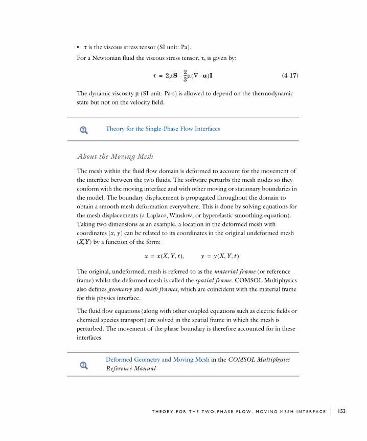
• τ is the viscous stress tensor (SI unit: Pa).

For a Newtonian fluid the viscous stress tensor, τ, is given by:

(4-17)

The dynamic viscosity μ (SI unit: Pa·s) is allowed to depend on the thermodynamic state but not on the velocity field.

About the Moving Mesh

The mesh within the fluid flow domain is deformed to account for the movement of the interface between the two fluids. The software perturbs the mesh nodes so they conform with the moving interface and with other moving or stationary boundaries in the model. The boundary displacement is propagated throughout the domain to obtain a smooth mesh deformation everywhere. This is done by solving equations for the mesh displacements (a Laplace, Winslow, or hyperelastic smoothing equation). Taking two dimensions as an example, a location in the deformed mesh with coordinates (x, y) can be related to its coordinates in the original undeformed mesh (X,Y) by a function of the form:

The original, undeformed, mesh is referred to as the material frame (or reference frame) whilst the deformed mesh is called the spatial frame. COMSOL Multiphysics also defines geometry and mesh frames, which are coincident with the material frame for this physics interface.

The fluid flow equations (along with other coupled equations such as electric fields or chemical species transport) are solved in the spatial frame in which the mesh is perturbed. The movement of the phase boundary is therefore accounted for in these interfaces.

τ 2μS 23---μ ∇ u⋅( )I–=

Theory for the Single-Phase Flow Interfaces

x x X Y t, ,( ) y, y X Y t, ,( )= =

Deformed Geometry and Moving Mesh in the COMSOL Multiphysics Reference Manual

T H E O R Y F O R T H E T W O - P H A S E F L O W , M O V I N G M E S H I N T E R F A C E | 153

154 | C H A P T E

About the Fluid Interface Boundary Conditions

The interfaces between phases are tracked with specific boundary conditions for the mesh displacement and the fluid flow. Two options are available — External Fluid Interface and Fluid-Fluid Interface. The External Fluid Interface boundary condition is appropriate when the viscosity of the external fluid is negligible compared to that of the internal fluid. In this case the pressure of the external fluid is the only parameter required to model the fluid and the flow is not solved for in the external fluid. For a fluid-fluid interface the flow is solved for both phases.

F L U I D - F L U I D I N T E R F A C E

The boundary conditions applied at an interface between two immiscible fluids, fluid 1 and fluid 2 (see Figure 4-2), are given by (Ref. 1):

(4-18)

(4-19)

(4-20)

where u1 and u2 are the velocities of the fluids 1 and 2 respectively, umesh is the velocity of the mesh at the interface between the two fluids, ni is the normal of the interface (outward from the domain of fluid 1), τ1 and τ2 are the total stress tensors in domains 1 and 2 respectively, fst is the force per unit area due to the surface tension and Mf is the mass flux across the interface (SI unit: kg/(m2s)).

Figure 4-2: Definition of fluid 1 and fluid 2 and the interface normal.

u1 u21ρ1------ 1

ρ2------

–

Mfni+=

ni τ2⋅ ni τ1⋅ fst+=

umesh u1 ni⋅Mf ρ1---------–

ni=


The tangential components of Equation 4-18 enforce a no-slip condition between the fluids at the boundary. In the absence of mass transfer across the boundary, Equation 4-18 and Equation 4-20 ensure that the fluid velocity normal to the boundary is equal to the velocity of the interface. When mass transfer occurs these equations result from conservation of mass and are easily derived in the frame where the boundary is stationary.

The components of the total stress tensor, τuv, represent the uth component of the force per unit area perpendicular to the v-direction. n·τ=nv τuv (using the summation convention) is therefore interpreted as the force per unit area acting on the boundary - in general this is not normal to the boundary. Equation 4-19 therefore expresses the force balance on the interface between the two fluids.

The force due to the surface tension is given by the following expression:

(4-21)

where ∇s is the surface gradient operator (∇s = (I − ni niT)∇ where I is the identity

matrix) and σ is the surface tension at the interface.

In the two dimensional case it is straightforward to see the physical origin of Equation 4-21. Consider an element of the surface of unit depth into the page as shown in Figure 4-3. The normal force per unit area Fn on the element in the limit δs → 0 is:

Because Rδθ → δs in the limit,

The quantity ∇s·ni in the first term on the right-hand side of Equation 4-21 is related to the mean curvature, κ, of the surface by the equation κ=−∇s·ni. In two dimensions the mean curvature κ = −1/R so ∇s·ni = 1/R. The first term in Equation 4-21 is therefore the normal force per unit area acting on the boundary due to the surface tension.

Two boundary conditions (Equation 4-18 and Equation 4-19) are necessary to couple the two domains as there are two separate sets of Navier-Stokes equations, one set for each of the domains.

fst σ ∇s ni⋅( )ni ∇sσ–=

Fnδs σ δσ+( ) δθ( )sin σδθ→=

FnσR----=


156 | C H A P T E

The tangential force per unit area, Ft, acting on the interface in Figure 4-3 can be obtained from the force balance along the direction of δs in the limit δs → 0:

This is equivalent to the second term on the right of Equation 4-21.

To obtain additional insight into the boundary condition, it is helpful to re-write Equation 4-19 as

assuming Newtonian fluids with viscosities μ1 and μ2 for fluids 1 and 2, respectively, and that p1 and p2 are the pressures in the respective fluids adjacent to the boundary. This equation expresses the equality of two vector quantities. It is instructive to consider the components perpendicular and tangential to the boundary. In the direction of the boundary normal

(4-22)

whereas in the tangential direction, ti,

(4-23)

Ftδs σ δσ+( ) δθ( ) σ–cos σ δσ+( ) σ–→=

Ftσ δσ+( ) σ–

δs-----------------------------→

ni p1 p2–( )I μ1– u∇ 1 u∇ 1( )T–( ) μ2 u∇ 2 u∇ 2( )T

–( )+( )⋅ σ ∇s ni⋅( )ni ∇sσ–=

p1 p2– n+ i μ2 u∇ 2 u∇ 2( )T–( ) μ1 u∇ 1 u∇ 1( )T

–( )–( ) ni⋅ ⋅ σ ∇s ni⋅( )ni=

ni μ2 u∇ 2 u∇ 2( )T–( ) μ1 u∇ 1 u∇ 1( )T

–( )–( ) ti⋅ ⋅ ∇sσ=


Figure 4-3: Diagrammatic representation of the forces acting on an element of a two-dimensional curved surface.

For the case of a static interface, Equation 4-22 expresses the pressure difference across the interface that results from its curvature. For a moving interface, the surface tension balances the difference in the total normal stress on either side of the interface.

Equation 4-23 involves only velocity gradients and the gradient of the surface tension. The implication of this is that surface tension gradients always drive motion; this is known as the Marangoni effect.

E X T E R N A L F L U I D I N T E R F A C E

It is often the case that the viscosity of fluid 1 is significantly greater than that of fluid 2 (for example for a liquid-vapor interface). In this case, the viscosity terms in the total stress from fluid 2 can be neglected and Equation 4-19 becomes:

(4-24)

The outer fluid (fluid 2) now enters the equation system only through the pressure term and the system can be represented by a domain consisting solely of the fluid 1 domain with an expression (or constant value) for the external pressure, pext, in the fluid 2 domain. Since the velocity in fluid 2 does not affect fluid 1, fluid 2 does not need to be explicitly modeled and Equation 4-18 can be dropped.

ni τ1⋅ pextn– i fst+=


158 | C H A P T E

Wall-Fluid Interface Boundary Conditions

At a three-phase boundary, it is necessary to add force terms on the boundary to ensure that the fluid maintains a consistent contact angle. Additionally the Wall boundary condition with the Navier Slip option must be used on the walls. The forces acting on the contact point are applied to the model by the Wall-Fluid Interface node.

Figure 4-4: Forces per unit length acting on a fluid-fluid interface at a three phase boundary with a solid wall. The surface tension force per unit length, σ, is balanced by a reaction force per unit length at the surface, Fn, and by the forces generated by the surface energies of the two phases at the interface: γs1 and γs2.

In equilibrium, the surface tension forces and the normal restoring force from the surface are in balance at a constant contact angle (θc), as shown in Figure 4-4. This equilibrium is expressed by Young's equation, which considers the components of the forces in the plane of the surface:

(4-25)

where σ is the surface tension force between the two fluids, γs1 is the surface energy density on the fluid 1 — solid interface and γs2 is the surface energy density on the fluid 2 — solid interface.

There is still debate in the literature as to precisely what occurs in non-equilibrium situations (for example, drop impact) when the physical contact angle deviates from the contact angle specified by a simple application of Young’s equation. A simple approach is to assume that the unbalanced part of the in plane Young Force acts on the fluid to move the contact angle towards its equilibrium value (Ref. 2). COMSOL

σ θc( )cos γs1+ γs2=


Multiphysics employs this approach as it is physically motivated and is consistent with the allowed form of the boundary condition from thermodynamics (Ref. 3, Ref. 4).

The normal force balance at the solid surface is handled by the wall boundary condition, which automatically prevents fluid flow across the solid boundary by the application of a constraint force. The wall-fluid interface feature applies a force on the fluid at the interface, fwf, with magnitude:

where θ is the actual contact angle and ms is the binormal to the solid surface, as defined in Figure 4-5.

Figure 4-5: Diagram showing normal and tangential vectors defined on the interface between two fluids and a solid surface in 3D (left) and 2D (right). The following vectors are defined: ni, the fluid-fluid interface unit normal; ns, the solid surface unit normal; tc, the tangent to the three-phase contact line; and mi and ms, the two unit binormals, which are defined as mi=tc×ni and ms=tc×ns, respectively.

References for the Two-Phase Flow, Moving Mesh Interface

1. R. Scardovell and S. Zalesk, “Direct Numerical Simulation of Free Surface and Interfacial Flow,” Annu. Rev. Fluid Mech., vol. 31, pp. 567–60, 1999.

2. J. Gerbeau and T. Lelievre, “Generalized Navier Boundary Condition and Geometric Conservation Law for Surface Tension,” Computer Methods In Applied Mechanics and Engineering, vol. 198, pp. 644–656, 2009.

fwf σ θc( )cos θ( )cos–( )ms=


160 | C H A P T E

3. W. Ren and E. Weinan, “Boundary Conditions for the Moving Contact Line Problem”, Physics of Fluids, vol. 19, p. 022101, 2007.

4. W. Ren and D. Hu, “Continuum Models for the Contact Line Problem”, Physics of Fluids, vol. 22, p. 102103, 2010.


5

M a t h e m a t i c s , M o v i n g I n t e r f a c e s

The Level Set and Phase Field Moving Interfaces are available under the Mathematics>Moving Interface branch ( ) when adding interfaces. See Modeling Microfluidic Fluid Flows to help you select which interface to use.

• The Level Set Interface

• The Phase Field Interface

• The Ternary Phase Field Interface

• Theory for the Level Set Interface

• Theory for the Phase Field Interface

• Theory for the Ternary Phase Field Interface

161

162 | C H A P T E

Th e L e v e l S e t I n t e r f a c e

The Level Set (ls) interface ( ), found under the Mathematics>Moving Interface branch ( ) when adding an interface, is used to track moving interfaces in fluid-flow models by solving a transport equation for the level set function. Simulations using the Level Set interface are always time dependent since the position of an interface almost always depends on its history.

The main node is the Level Set Model feature, which adds the level set equation and provides an interface for defining the level set properties and the velocity field.

When this physics interface is added, the following default nodes are also added in the Model Builder — Level Set Model, No Flow (the default boundary condition) and Initial

Values. Then, from the Physics toolbar, add other nodes that implement, for example, boundary conditions. You can also right-click Level Set to select physics features from the context menu.

S E T T I N G S


The Name is used primarily as a scope prefix for variables defined by the physics interface. Refer to such physics interface variables in expressions using the pattern <name>.<variable_name>. In order to distinguish between variables belonging to different physics interfaces, the name string must be unique. Only letters, numbers, and underscores (_) are permitted in the Name field. The first character must be a letter.

The default Name (for the first physics interface in the model) is ls.

S T A B I L I Z A T I O N

To display this sections, click the Show button ( ) and select Stabilization.

There are two stabilization methods available — Streamline diffusion and Crosswind

diffusion. Both are active by default and should remain selected for optimal performance.


To display this sections, click the Show button ( ) and select Advanced settings

options.

Specify the Convective term as Nonconservative form (default) or Conservative form.

R 5 : M A T H E M A T I C S , M O V I N G I N T E R F A C E S


By default, the Level Set interface uses Linear elements. When coupling the physics interface to a fluid flow interface by means of the T he Two-Phase Flow, Level Set Coupling Feature, exact conservation of the integral of is obtained using the nonconservative form provided that the discretization order of the level set variable is equal to or lower than the order of the pressure.


The dependent variable (field variable) is the Level set variable phi. The name can be changed but the names of fields and dependent variables must be unique within a model.

Domain, Boundary, and Pair Nodes for the Level Set Interface

The Level Set Interface has the following domain, boundary and pair nodes described.

φ

• Conservative and Nonconservative Form

• Domain, Boundary, and Pair Nodes for the Level Set Interface

• Theory for the Level Set Interface


• Initial Interface

• Initial Values

• Inlet

• Level Set Model

• No Flow

• Outlet1

• Periodic Condition (see Periodic Boundary Conditions in the COMSOL Multiphysics Reference Manual)

• Symmetry1

• Thin Barrier

1 Described for the Laminar Flow interface.

Boundary conditions for axial symmetry boundaries are not required. For the symmetry axis at r = 0, the software automatically provides a suitable boundary condition and adds an Axial Symmetry node that is valid on the axial symmetry boundaries only.

T H E L E V E L S E T I N T E R F A C E | 163

164 | C H A P T E

Level Set Model

The Level Set Model node adds the following transport equation governing a level set function

and provides the options to define the associated level set parameters and the velocity field.

L E V E L S E T P A R A M E T E R S

Enter a value or expression for the Reinitialization parameter γ (SI unit: m/s). The default is 1 m/s.

Enter a value or expression for the Parameter controlling interface thickness els (SI unit: m). The default expression is ls.hmax/2, which means that the value is half of the maximum mesh element size in the region through which the interface passes.

C O N V E C T I O N

Enter values or expressions for the components (u, v, and w in 3D, for example) of the Velocity field u (SI unit: m/s). The applied velocity field transports the level set function through convection.

Initial Values

Use the Initial Values node to define the initial values of the level set variable.


The initial positions of the two fluids, and consequently the separating interface, can be specified in two ways. The level set function can be specified explicitly, using any type of variable or expression. Alternatively the fluid occupying the current domain selection can be specified. Using the former method, a Time Dependent study step can


φ

t∂∂φ u φ∇⋅+ γ∇ ε∇φ φ 1 φ–( ) ∇φ

∇φ----------–

⋅=


directly be solved. Using the latter method, a Phase Initialization study step is needed in order to initialize the level set function across the fluid-fluid interface.

Specify the Level set variable as one of the following:

• To specify the fluid occupying the domain, select Specify phase (default). Then select the check box Fluid 1 ( ) or Fluid 2 ( ).

• For User defined enter a value or expression for the level set variable .

Inlet

S E T T I N G S

Specify Level Set Condition according to one of the following options:

• Fluid 1 ( )

• Fluid 2 ( )

• Specify level set function explicitly

When the Specify level set function explicitly is selected, the level set function must be specified in the entire domain. The value must be in the range from 0 to 1, where the default is 0.

φ 0= φ 1=

φ

If the Phase Initialization ( ) study step is being used, for the initialization to work it is crucial that there are two Initial Values nodes and one Initial Interface node. The Initial Values nodes should specify the Level set variable as Specify phase: Fluid 1 and Specify phase: Fluid 2 respectively. The Initial Interface node should include all interior boundaries that define the initial position of the fluid-fluid interface. If the selection of the Initial interface node is empty, the initialization fails.

See Initializing the Level Set Function.

φ 0=

φ 1=

φ

T H E L E V E L S E T I N T E R F A C E | 165

166 | C H A P T E

Initial Interface

The Initial Interface node defines the boundary as the initial position of the interface .

No Flow

The No Flow node adds a boundary condition that represents boundaries where there is no flow across the boundary. This is the default boundary condition.

Thin Barrier

The Thin Barrier feature is available on interior boundaries and introduces a discontinuity in the level set variable across the boundary. A No Flow condition is prescribed on each side. This node can be used to avoid meshing thin structures.

φ 0=

If the Transient with Initialization ( ) study is being used, for the initialization to work it is crucial that there are two Initial Values nodes and one Initial Interface node. One of the Initial Values nodes should use Specify phase: Fluid 1 and the other Specify phase: Fluid 2. The Initial Interface node should have all interior boundaries where the interface is initially present as selection. If the selection of the Initial interface node is empty, the initialization fails.

See Initializing the Level Set Function.


Th e Pha s e F i e l d I n t e r f a c e

The Phase Field (pf) interface ( ), found under the Mathematics>Moving Interface branch ( ) when adding a physics interface, is used to track moving interfaces by solving two transport equations, one for the phase field variable, , and one for the mixing energy density, ψ. The position of the interface is determined by minimizing the free energy.

The main node is the Phase Field Model feature, which adds the phase field equations and provides an interface for defining the phase field model properties.

When this physics interface is added, the following default nodes are also added in the Model Builder — Phase Field Model, Wetted Wall (the default boundary condition) and Initial Values. Then, from the Physics toolbar, add other nodes that implement, for example, boundary conditions. You can also right-click Phase Field to select physics features from the context menu.

S E T T I N G S



The default Name (for the first physics interface in the model) is pf.


To display this sections, click the Show button ( ) and select Advanced settings

options.

Specify the Convective term as Nonconservative form (default) or Conservative form.


By default, the Phase Field interface uses Linear elements.

φ

T H E P H A S E F I E L D I N T E R F A C E | 167

168 | C H A P T E


This interface defines the dependent variables (fields) Phase field variable and Phase

field help variable ψ. If required, edit the name, but dependent variables must be unique within a model.

Domain, Boundary, and Pair Nodes for the Phase Field Interface

The Phase Field Interface includes the following domain, boundary, and pair nodes, listed in alphabetical order, available from the Physics ribbon toolbar (Windows users), Physics context menu (Mac or Linux users), or right-click to access the context menu (all users).

φ

• Conservative and Nonconservative Forms

• Domain, Boundary, and Pair Nodes for the Phase Field Interface

• Theory for the Phase Field Interface

In general, to add a node, go to the Physics toolbar, no matter what operating system you are using. Subnodes are available by clicking the parent node and selecting it from the Attributes menu.

• Initial Interface

• Initial Values

• Inlet

• Interior Wetted Wall

• Outlet1

• Periodic Condition (see Periodic Boundary Conditions in the COMSOL Multiphysics Reference Manual)

• Phase Field Model

• Symmetry1

• Wetted Wall

1 Described for the Laminar Flow interface.



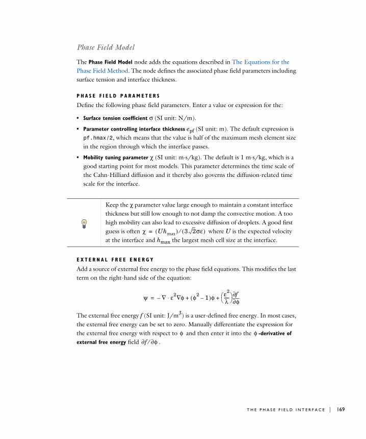
Phase Field Model

The Phase Field Model node adds the equations described in The Equations for the Phase Field Method. The node defines the associated phase field parameters including surface tension and interface thickness.

P H A S E F I E L D P A R A M E T E R S

Define the following phase field parameters. Enter a value or expression for the:

• Surface tension coefficient σ (SI unit: N/m).

• Parameter controlling interface thickness epf (SI unit: m). The default expression is pf.hmax/2, which means that the value is half of the maximum mesh element size in the region through which the interface passes.

• Mobility tuning parameter χ (SI unit: m·s/kg). The default is 1 m·s/kg, which is a good starting point for most models. This parameter determines the time scale of the Cahn-Hilliard diffusion and it thereby also governs the diffusion-related time scale for the interface.

E X T E R N A L F R E E E N E R G Y

Add a source of external free energy to the phase field equations. This modifies the last term on the right-hand side of the equation:

The external free energy f (SI unit: J/m3) is a user-defined free energy. In most cases, the external free energy can be set to zero. Manually differentiate the expression for the external free energy with respect to and then enter it into the -derivative of

external free energy field .

Keep the χ parameter value large enough to maintain a constant interface thickness but still low enough to not damp the convective motion. A too high mobility can also lead to excessive diffusion of droplets. A good first guess is often where U is the expected velocity at the interface and hmax the largest mesh cell size at the interface.

χ Uhmax( ) 3 2σε( )⁄=

ψ ∇ ε2 φ∇⋅– φ2 1–( )φ ε2

λ-----

φ∂∂f

+ +=

φ φ∂f ∂φ⁄


170 | C H A P T E

C O N V E C T I O N

Enter values or expressions for the components (u, v, and w in 3D, for example) of the Velocity field u (SI unit: m/s). The applied velocity field transports the phase field variables through convection.

Initial Values

Use the Initial Values node to define the initial values of the phase field variable.


The initial positions of the two fluids, and consequently the fluid-fluid interface, can be specified in two ways. The phase field variable can be specified explicitly, using any type of variable or expression. Alternatively the fluid occupying the current domain selection can be specified. Using the former method, a Time Dependent study step can directly be solved. Using the latter method, a Phase Initialization study step is needed in order to initialize the phase field function across the fluid-fluid interface.

Specify the Phase field variable as one of the following:

• To specify the fluid occupying the domain, select Specify phase (default). Then select the check box Fluid 1 ( ) or Fluid 2 ( ).

• For User defined enter a value or expression for the phase field variable .

Additional Sources of Free Energy

φ 1–= φ 1=

φ

If the Phase Initialization ( ) study step is being used, for the initialization to work it is crucial that there are two Initial Values nodes and one Initial Interface node. The Initial Values nodes should specify the Phase field variable as Specify phase: Fluid 1 and Specify phase: Fluid 2 respectively. The Initial Interface node should include all interior boundaries that defines the initial position of the fluid-fluid interface. If the selection of the Initial interface node is empty, the initialization will fail.


Inlet

S E T T I N G S

Specify Phase field Condition according to one of the following options:

• Fluid 1 ( )

• Fluid 2 ( )

• Specify phase field function explicitly

When Specify phase field function explicitly is selected, the phase field function must be specified in the entire domain. The value must be in the range from -1 to 1, where the default is 1.

Initial Interface

The Initial Interface node defines the boundary as the initial position of the interface .

Wetted Wall

The Wetted Wall node is the default boundary condition representing wetted walls. Along a wetted wall the contact angle for the fluid, θw, is specified, and across it, the mass flow is zero. This is prescribed by

in combination with

φ 1–=

φ 1=

φ

φ 0=

If the Transient with Phase Initialization ( ) study is being used, for the initialization to work it is crucial that there are two Initial Values nodes and one Initial Interface node. One of the Initial Values nodes is set to Specify

phase: Fluid 1 and the other to Specify phase: Fluid 2. The Initial Interface node should have all interior boundaries where the interface is initially present as selection. If the selection of the Initial Interface node is empty, the initialization fails.

n ε2 φ∇⋅ ε2 θw( )cos φ∇=

n γλε2------ ψ∇⋅ 0=


172 | C H A P T E

W E T T E D W A L L

Enter a value or expression for the Contact angle θw. The default value is π/2 rad.

Interior Wetted Wall

The Interior Wetted Wall feature is available on interior boundaries. It is similar to the Wetted Wall condition except that it applies on both sides of an internal boundary and introduces a discontinuity of the phase field variables across the boundary. This node can be used to avoid meshing thin structures.

Along an interior wetted wall the contact angle for the fluid, θw, is specified on both sides of the boundary, and across it, the mass flow is zero.

W E T T E D W A L L

Enter a value or expression for the Contact angle θw. The default value is π/2 rad.


Th e T e r n a r y Pha s e F i e l d I n t e r f a c e

The Ternary Phase Field (terpf) interface ( ), found under the Mathematics>Moving

Interface branch ( ) when adding a physics interface, is used to track moving interfaces separating three different phases. The interface solves four transport equations: two equations governing phase field variables, and , and two equations for the corresponding generalized chemical potentials, ηA and ηB. The position of the interfaces are determined by minimization of the free energy.

The phase field variables are defined such that they represent the volume fraction of the respective phase. The volume fraction of the third phase not solved for, but computed from the natural constraint that the sum of the volume fractions of all phases is one.

The main node of the interface is the Phase Field Model feature, which adds the phase field equations and provides an interface for defining the phase field model properties such as surface tensions and parameters controlling the interface thickness.

When this physics interface is added, the following default nodes are also added in the Model Builder — Mixture Properties, Wetted Wall and Initial Values. Then, from the Physics toolbar, add other nodes that implement, for example, boundary conditions. You can also right-click Ternary Phase Field to select physics features from the context menu.

S E T T I N G S



The default Name (for the first physics interface in the model) is terpf.


This interface defines the dependent variables (fields):

• Phase field variable, fluid A phiA

• Phase field variable, fluid B phiB

φA φB

T H E T E R N A R Y P H A S E F I E L D I N T E R F A C E | 173

174 | C H A P T E

• Generalized chemical potential of fluid A etaA

• Generalized chemical potential of fluid B etaB

If required, edit the any of the names, but dependent variables must be unique within a model.

Domain, Boundary, and Pair Nodes for the Ternary Phase Field Interface

The Ternary Phase Field Interface includes the following domain, boundary, and pair nodes, listed in alphabetical order, available from the Physics ribbon toolbar (Windows users), Physics context menu (Mac or Linux users), or by right-clicking the interface node to access the context menu (all users).

Mixture Properties

The Mixture Properties node adds the equations described in The Equations of the Ternary Phase Field Method. The node defines the associated phase field parameters, including the surface tension coefficients and parameters controlling the thickness of the interfaces.


The surface tension coefficients can be defined through user inputs, variables, or by selecting a material. For the latter option, an additional input, the temperature, may be required to define these properties.

TemperatureBy default, the Temperature model input is set to Common model input, and the temperature is controlled from Common Model Inputs under Global Definitions or by a locally defined Model Input. If a Heat Transfer interface is included in the

Theory for the Ternary Phase Field Interface

• Initial Values

• Inlet

• Outlet

• Phase Field Model

• Symmetry

• Wetted Wall


component, it controls the temperature Common model input. Alternatively, the temperature field can be selected from another physics interface. All physics interfaces have their own tags (Name). For example, if a Heat Transfer in Fluids interface is included in the component, the Temperature (ht) option is available for T.

You can also select User defined from the Temperature model input in order to manually prescribe T

P H A S E F I E L D P A R A M E T E R S

Define the following phase field parameters. Enter a value or expression for the:

• Parameter controlling interface thickness ε. The default expression applied is terpf.hmax*sqrt(2), which means that the thickness is related to the maximum mesh element size in the domain. If the element size in the regions passed by the interfaces is known beforehand, it is recommended to apply a value of ε in that order.

• Mobility tuning parameter M0. This parameter determines the time scale of the Cahn-Hilliard diffusion and it thereby also governs the diffusion-related time scale for the interface. Keep the mobility tuning parameter value large enough to maintain a constant interface thickness but still low enough to not damp the convective motion. A too high mobility can also lead to excessive diffusion of droplets. By default, M0 is set to 1·10-4 m3/s, which is a good starting point for most models.

• Additional free bulk energy Λ. When needed, add a user-defined expression for the additional bulk energy.


Specify the surface tension coefficients for the three types of interfaces present.

• To use a predefined expression, select Library coefficient, liquid/gas interface or Library coefficient, liquid/liquid interface. Then select an option from the list that displays below (Water/Air, Glycerol/Air, and so forth).

• For User defined, enter a value or expression for the surface tension coefficient.



176 | C H A P T E

C O N V E C T I O N

Enter values or expressions for the components (u, v, and w in 3D, for example) of the Velocity field u. The applied velocity field transports the phase field variables through convection.

Initial Values

The Initial Values node adds initial values for the phase field variables that can serve as initial conditions for a transient simulation.


Enter initial values or expressions for Phase field variable A and the Phase field variable

B corresponding to the mass fraction of the respective phase. The value must be in the range from 0 to 1.

Inlet

This condition should be used on boundaries for which there is a net convective flow of the phases into the adjacent domain.

I N L E T

Specify phase field variables, corresponding to the volume fractions, of phase A and phase B. The value must be in the range from 0 to 1. The volume fraction of phase C will be evaluated such that the sum of all mass fractions equals one.

Mathematically this boundary condition imposes

,

for phases i = A and B.

Outlet

This condition should be used on boundaries for which there is a net convective outflow from the domain.


φi φi 0,= nM0Σi-------- ηi∇⋅ 0=

nM0Σi-------- ηi∇⋅ 0=



Symmetry

Use this condition on boundaries that represent a geometrical symmetry line across which the flow of the fluid phases is zero.



Wetted Wall

Use this node to represent a solid wall along which the contact angles between the separating interfaces and the wall should be prescribed.

W E T T E D W A L L

Enter values or expressions for the contact angles for the three interfaces types:

• The Contact angle of interface from phase A to phase C θα.

• The Contact angle of interface from phase B to phase C θβ.

• The Contact angle of interface from phase A to phase B θγ.

nM0Σi-------- ηi∇⋅ 0=


178 | C H A P T E

The definition of the contact angles with respect to the wall are shown in the figure below

Figure 5-1: Definitions of the contact angels in the Wetted Wall feature of the Ternary Phase Field interface.


Th eo r y f o r t h e L e v e l S e t I n t e r f a c e

Fluid flow with moving interfaces or boundaries occur in a number of different applications, such as fluid-structure interaction, multiphase flows, and flexible membranes moving in a liquid. One way to track moving interfaces is to use a level set method. A certain contour line of the globally defined function, the level set function, then represents the interface between the phases. For The Level Set Interface the fluid-fluid interface can be advected with an arbitrary velocity field.

In this section:

• The Level Set Method

• Conservative and Nonconservative Form

• Initializing the Level Set Function

• Variables For Geometric Properties of the Interface

• Reference for the Level Set Interface

The Level Set Method

The level set method is a technique to represent moving interfaces or boundaries using a fixed mesh. It is useful for problems where the computational domain can be divided into two domains separated by an interface. Each of the two domains can consist of several parts. Figure 5-2 shows an example where one of the domains consists of two separated parts. The interface is represented by a certain level set or isocontour of a globally defined function, the level set function . In COMSOL Multiphysics, is a smooth step function that equals zero (0) in one domain and one (1) in the other. Across the interface, there is a smooth transition from zero to one. The interface is

φ φ

T H E O R Y F O R T H E L E V E L S E T I N T E R F A C E | 179

180 | C H A P T E

defined by the 0.5 isocontour, or level set, of . Figure 5-3 shows the level set representation of the interface in Figure 5-2.

Figure 5-2: An example of two domains divided by an interface. In this case, one of the domains consists of two parts. Figure 5-3 shows the corresponding level set representation.

Figure 5-3: A surface plot of the level set function corresponding to Figure 5-2.

The physics interface solves Equation 5-1 in order to move the interface with the velocity field u:

(5-1)

The terms on the left-hand side give the correct motion of the interface, while those on the right-hand side are necessary for numerical stability. The parameter, ε, determines the thickness of the region where varies smoothly from zero to one and is typically of the same order as the size of the elements of the mesh. By default, ε is

φ

t∂∂φ u φ∇⋅+ γ∇ ε∇φ φ 1 φ–( ) ∇φ

∇φ----------–

⋅=

φ


constant within each domain and equals the largest value of the mesh size, h, within the domain. The parameter γ determines the amount of reinitialization or stabilization of the level set function. It needs to be tuned for each specific problem. If γ is too small, the thickness of the interface might not remain constant and oscillations in can appear because of numerical instabilities. On the other hand, if γ is too large the interface moves incorrectly. A suitable value for γ is the maximum magnitude of the velocity field u.

Conservative and Nonconservative Form

If the velocity is divergence free, that is, if

(5-2)

the volume (area for 2D problems) bounded by the interface should be conserved if there is no inflow or outflow through the boundaries. To obtain exact numerical conservation in cases where Equation 5-2 is not fully satisfied, switch to the conservative form

(5-3)

in Settings window for The Level Set Interface.

Using the conservative level set form, exact numerical conservation of the integral of is obtained. However, the nonconservative form is better suited for numerical

calculations and usually converges more easily. The nonconservative form, which is the default form, only conserves the integral of the level set function approximately, but this is sufficient for most applications.

When the Level Set interface is coupled to a fluid flow interface by means of T he Two-Phase Flow, Level Set Coupling Feature, exact conservation of the integral of is obtained using the nonconservative form provided that the discretization order of the level set variable is equal to or lower than the order of the pressure.

φ

∇ u⋅ 0=

t∂∂φ ∇ uφ( )⋅+ γ∇ ε∇φ φ 1 φ–( ) ∇φ

∇φ----------–

⋅=

φ

φ

Rising Bubble: path CFD_Module/Multiphase_Tutorials/rising_bubble_2daxi


182 | C H A P T E

Initializing the Level Set Function

If the study type Transient with Phase Initialization is used in the model, the level set variable is first initialized so that it varies smoothly between zero and one over the interface. For that study, two study steps are created, Phase Initialization and Time Dependent. The Phase Initialization step solves for the distance to the initial interface, Dwi. The Time Dependent step then uses the initial condition for the level set function according to the following expression:

in domains initially outside the interface and

in domains initially inside the interface. Here, inside refers to domains where and outside refers to domains where .

Variables For Geometric Properties of the Interface

Geometric properties of the interface are often needed. The unit normal to the interface is given by

(5-4)

φ01

1 eDwi ε⁄–

+--------------------------=

φ01

1 eDwi ε⁄

+------------------------=

φ 0.5<φ 0.5>

For the initialization to work it is crucial that there are two Initial Values nodes and one Initial Interface node. One of the Initial Values nodes should use Specify phase: Fluid 1 ( ) and the other Specify phase: Fluid

2 ( ). The Initial Interface node should have all interior boundaries where the interface is initially present as selection. If the selection of the Initial interface node is empty, the initialization fails.

• The Level Set Interface

• Studies and Solvers and Time Dependent with Initialization in the COMSOL Multiphysics Reference Manual

φ 0=

φ 1=

n ∇φ∇φ----------

φ 0.5=

=


This variable is available in the physics interface as the interface normal ls.intnorm.

Reference for the Level Set Interface

1. E. Olsson and G. Kreiss, “A Conservative Level Set Method for Two Phase Flow,” J. Comput. Phys., vol. 210, pp. 225–246, 2005.


184 | C H A P T E

Th eo r y f o r t h e Pha s e F i e l d I n t e r f a c e

The Phase Field Interface theory is described in this section:

• About the Phase Field Method

• The Equations for the Phase Field Method

• Conservative and Nonconservative Forms

• Additional Sources of Free Energy

• Initializing the Phase Field Function

• Variables and Expressions

• Reference for the Phase Field Interface

About the Phase Field Method

The phase field method offers an attractive alternative to more established methods for solving multiphase flow problems. Instead of directly tracking the interface between two fluids, the interfacial layer is governed by a phase field variable, . The surface tension force is added to the Navier-Stokes equations as a body force by multiplying the chemical potential of the system by the gradient of the phase field variable.

The evolution of the phase field variable is governed by the Cahn-Hilliard equation, which is a 4th-order PDE. The Phase Field interface decomposes the Cahn-Hilliard equation into two second-order PDEs.

For the level set method, the fluid interface is simply advected with the flow field. The Cahn-Hilliard equation, on the other hand, does not only convect the fluid interface, but it also ensures that the total energy of the system diminishes correctly. The phase field method thus includes more physics than the level set method.

The free energy of a system of two immiscible fluids consists of mixing, bulk distortion, and anchoring energy. For simple two-phase flows, only the mixing energy is retained, which results in a rather simple expression for the free energy.

The Equations for the Phase Field Method

The free energy is a functional of a dimensionless phase field parameter, :

φ

φ


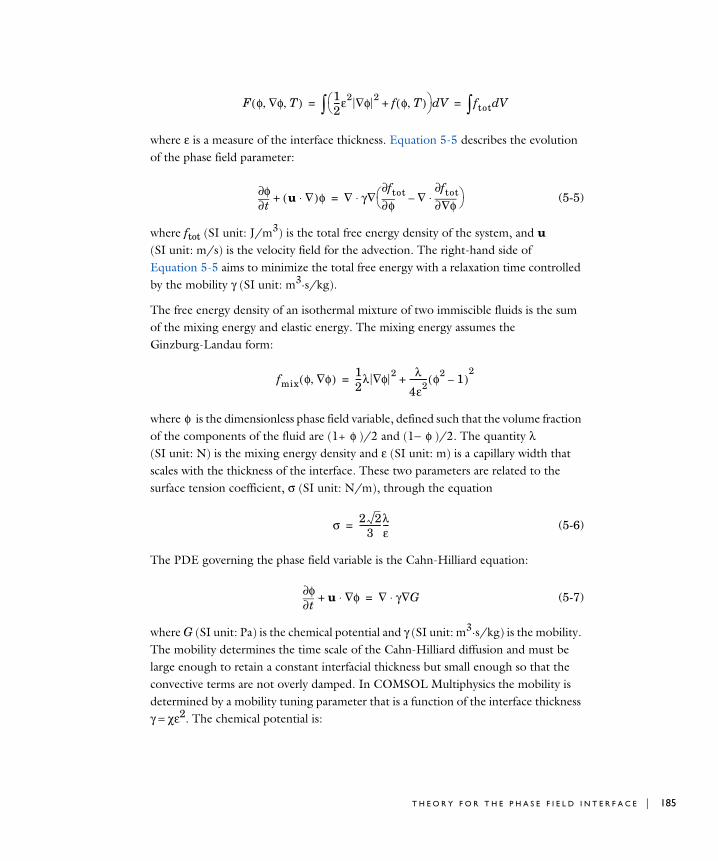
where ε is a measure of the interface thickness. Equation 5-5 describes the evolution of the phase field parameter:

(5-5)

where ftot (SI unit: J/m3) is the total free energy density of the system, and u (SI unit: m/s) is the velocity field for the advection. The right-hand side of Equation 5-5 aims to minimize the total free energy with a relaxation time controlled by the mobility γ (SI unit: m3·s/kg).

The free energy density of an isothermal mixture of two immiscible fluids is the sum of the mixing energy and elastic energy. The mixing energy assumes the Ginzburg-Landau form:

where is the dimensionless phase field variable, defined such that the volume fraction of the components of the fluid are (1+ )/2 and (1− )/2. The quantity λ (SI unit: N) is the mixing energy density and ε (SI unit: m) is a capillary width that scales with the thickness of the interface. These two parameters are related to the surface tension coefficient, σ (SI unit: N/m), through the equation

(5-6)

The PDE governing the phase field variable is the Cahn-Hilliard equation:

(5-7)

where G (SI unit: Pa) is the chemical potential and γ (SI unit: m3·s/kg) is the mobility. The mobility determines the time scale of the Cahn-Hilliard diffusion and must be large enough to retain a constant interfacial thickness but small enough so that the convective terms are not overly damped. In COMSOL Multiphysics the mobility is determined by a mobility tuning parameter that is a function of the interface thickness γ = χε2. The chemical potential is:

F φ φ∇ T, ,( ) 12---ε2 φ∇ 2 f φ T,( )+ Vd ftot Vd= =

t∂∂φ u ∇⋅( )φ+ ∇ γ∇

φ∂∂ftot ∇

φ∇∂∂ftot⋅–

⋅=

fmix φ φ∇,( ) 12---λ φ∇ 2 λ

4ε2--------- φ2 1–( )

2+=

φφ φ

σ 2 23-----------λ

ε---=

t∂∂φ u φ∇⋅+ ∇ γ G∇⋅=

T H E O R Y F O R T H E P H A S E F I E L D I N T E R F A C E | 185

186 | C H A P T E

(5-8)

The Cahn-Hilliard equation forces to take a value of 1 or −1 except in a very thin region on the fluid-fluid interface. The Phase Field interface breaks Equation 5-7 up into two second-order PDEs:

(5-9)

(5-10)

Conservative and Nonconservative Forms

If the velocity field is divergence free, that is, if

(5-11)

the volume (area for 2D problems) bounded by the interface should be conserved if there is no inflow or outflow through the boundaries. To obtain exact numerical conservation in cases where Equation 5-11 is not fully satisfied, switch to the conservative form

Using the conservative phase field form, exact numerical conservation of the integral of is obtained. However, the nonconservative form is better suited for numerical calculations and usually converges more easily. The nonconservative form, which is the default form, only conserves the integral of the phase field function approximately, but this is sufficient for most applications.

When the Phase Field interface is coupled to a fluid flow interface by means of the The Two-Phase Flow, Phase Field Coupling Feature, conservation of the integral of using the nonconservative form can be improved provided that the discretization order of the phase field variables is equal to or lower than the order of the pressure.

G λ ∇2φ–φ φ2 1–( )

ε2-----------------------+=

φ

t∂∂φ u φ∇⋅+ ∇ γλ

ε2------∇ψ⋅=

ψ ∇ ε2 φ∇⋅– φ2 1–( )φ+=

∇ u⋅ 0=

t∂∂φ ∇ uφ⋅+ ∇ γλ

ε2------∇ψ⋅=

φ

φ


Additional Sources of Free Energy

In some cases, the expression for the free energy can include other sources. It is possible to incorporate these by modifying Equation 5-10:

(5-12)

where f is a user-defined free energy (SI unit: J/m3).

Initializing the Phase Field Function

If the study type Transient with Phase Initialization is used in the model, the phase field variable is first initialized so that it varies smoothly between zero and one over the interface. For this study, two study steps are created, Phase Initialization and Time Dependent. The Phase Initialization step solves for the distance to the initial interface, Dwi. The Time Dependent step then uses the initial condition for the phase field function according to the following expression:

in Fluid 1 and

ψ ∇ ε2 φ∇⋅– φ2 1–( )φ ε2

λ-----

φ∂∂f

+ +=

The expression for the external free energy must be manually differentiated with respect to and then entered into the field. In most cases, the external free energy is zero.

φ ∂f ∂φ⁄

φ0Dwi

2ε---------- tanh–=

φ0Dwi

2ε---------- tanh=

T H E O R Y F O R T H E P H A S E F I E L D I N T E R F A C E | 187

188 | C H A P T E

in Fluid 2. These expressions are based on a steady, analytic solution to Equation 5-9 and Equation 5-10 for a straight, non-moving interface.

Variables and Expressions

Unlike the level set method, the phase field method does not require expressions for the unit normal to the interface or smoothed delta functions, so they are not available for analysis. Variables that are defined are the chemical potential, which can be rewritten in terms of the dependent variable ψ,

and the surface tension force F = G∇ .

The mean curvature (SI unit: 1/m) of the interface can be computed by entering the following expression:

Reference for the Phase Field Interface

1. P. Yue, C. Zhou, J.J. Feng, C.F. Ollivier-Gooch, and H.H. Hu, “Phase-field Simulations of Interfacial Dynamics in Viscoelastic Fluids Using Finite Elements with Adaptive Meshing,” J. Comp. Phys., vol. 219, pp. 47–67, 2006.

If the Transient with Phase Initialization ( ) study is being used, for the initialization to work it is crucial that there are two Initial Values nodes and one Initial Interface node. One of the Initial Values nodes is set to Specify

phase: Fluid 1 and the other to Specify phase: Fluid 2. The Initial Interface node should have all interior boundaries where the interface is initially present as selection. If the selection of the Initial Interface node is empty, the initialization fails.

Studies and Solvers in the COMSOL Multiphysics Reference Manual

G λψε2-------=

φ

κ 2 1 φ+( ) 1 φ–( )Gσ----=


Th eo r y f o r t h e T e r n a r y Pha s e F i e l d I n t e r f a c e

The Ternary Phase Field Interface theory is described in this section:

• About the Phase Field Method

• The Equations of the Ternary Phase Field Method

• Reference for the Phase Field Interface

About the Phase Field Method

The phase field method offers an attractive alternative to more established methods for solving multiphase flow problems. Instead of directly tracking the interface between two fluids, the separating interface is identified as the region across which the phase field variables of the two adjacent phases varies between its two limiting values. The surface tension force is added to the Navier-Stokes equations as a body force by multiplying the chemical potentials of the phases by the gradient of the corresponding phase field variable.

The evolution of each phase field variable is governed by the Cahn-Hilliard equation, which is a 4th-order PDE. The Ternary Phase Field interface decomposes each Cahn-Hilliard equation into two second-order PDEs.

For the level set method, the fluid interface is simply advected with the flow field. The Cahn-Hilliard equation, on the other hand, does not only convect the fluid interface, but it also ensures that the total energy of the system diminishes correctly. The phase field method thus includes more physics than the level set method.

The free energy of a system of immiscible fluids consists of mixing, bulk distortion, and anchoring energy. For simple three-phase flows, only the mixing energy is retained.

The Equations of the Ternary Phase Field Method

The ternary phase field model implemented in COMSOL is based the work of Boyer and co-workers in Ref. 1. The model is designed in order to study the evolution of the three immiscible phases, denoted phase A, phase B, and phase C, respectively. Each phase is represented by a phase field variable , which takes values between 0 and 1. The phase field variables satisfies the constraint

φ

T H E O R Y F O R T H E T E R N A R Y P H A S E F I E L D I N T E R F A C E | 189

190 | C H A P T E

(5-13)

and density of each phase is assumed to be constant. This implies that the phase field variable corresponds directly to the volume fraction of the phase in question.

The free energy of the three phase system is defined as a function of the phase field variables in the manner of:

(5-14)

Here the σij denotes the surface tension coefficient of the interface separating phase i and j, and the capillary parameters Σi are defined as

(5-15)

and Λ is a function or parameter specifying the additional free bulk energy. By default Λ is zero. In this case it can be seen that the free energy in Equation 5-14 represents the mixing energy, since only interfaces between two phases (where two phase field variables varies between the limiting values) contributes to the free energy.

The Cahn-Hilliard equations to be solved for each phase p = A,B,C are

(5-16)

It can be noted that the Cahn-Hilliard equation is originally a 4th-order PDE. In COMSOL Multiphysics, that PDE is split up into two second-order PDEs by introducing an additional dependent variable, the generalized potential η, one for each phase. In order to satisfy Equation 5-14, two sets of the equations shown in Equation 5-16 are solved, those for phase A and phase B. The phase field variable, and correspondingly the mass fraction, for fluid C is computed from Equation 5-14.

In Equation 5-16 ε (SI unit: 1/m) is a parameter controlling the interface thickness, M0 (SI unit: m3/s) is a molecular mobility parameter, and the parameter ΣT is defined as

φi

i A B C, ,= 0=

F σABφA2 φB

2 σACφA2 φC

2 σBCφB2 φC

2+ + +=

φAφBφC ΣAφA ΣBφB ΣCφC+ +( ) ΛφA2 φB

2 φC2

+

Σi σij σik σjk–+=

∂φi∂t--------

∂ujφi∂xj-------------+

∂∂xj--------

M0Σi--------

∂ηi

∂xj--------

=

ηi4ΣT

ε---------- 1

Σj----- ∂F

∂φi-------- ∂F

∂φj--------–

3

4---εΣj

∂∂xj--------

∂ηi

∂xj-------- –

j i≠=


(5-17)

Reference for the Ternary Phase Field Interface

1. F. Boyer, C. Lapuerta, S. Minjeaud, B. Piar, and M. Quintard, “Cahn-Hilliard/Navier-Stokes model for the simulation of three-phase flows”, Transport in Porous Media, vol. 28, pp. 463–484, 2010.

3ΣT------ 1

ΣA------- 1

ΣB------- 1

ΣC-------+ +=

T H E O R Y F O R T H E T E R N A R Y P H A S E F I E L D I N T E R F A C E | 191

192 | C H A P T E

6

P o r o u s M e d i a F l o w I n t e r f a c e s

This chapter discusses the physics interfaces found under the Fluid Flow>Porous

Media and Subsurface Flow branch ( ). See Modeling Microfluidic Fluid Flows to help you select which physics interface to use.

In this chapter:

• The Darcy’s Law Interface

• The Brinkman Equations Interface

• The Free and Porous Media Flow Interface

• Theory for the Darcy’s Law Interface

• Theory for the Brinkman Equations Interface

• Theory for the Free and Porous Media Flow Interface

193

194 | C H A P T E

Th e Da r c y ’ s L aw I n t e r f a c e

The Darcy’s Law (dl) interface ( ), found under the Porous Media and Subsurface Flow branch ( ) when adding a physics interface, is used to simulate fluid flow through interstices in a porous medium. It can be used to model low-velocity flows or media where the permeability and porosity are very small, and for which the pressure gradient is the major driving force and the flow is mostly influenced by the frictional resistance within the pores. Set up multiple Darcy's Law interfaces to model multiphase flows involving more than one mobile phase. The Darcy’s Law interface can be used for stationary and time-dependent analyses.

The main feature is the Fluid and Matrix Properties node, which provides an interface for defining the fluid material along with the porous medium properties.

When this physics interface is added, the following default nodes are also added in the Model Builder — Fluid and Matrix Properties, No Flow (the default boundary condition), and Initial Values. Then, from the Physics toolbar, add other nodes that implement, for example, boundary conditions and mass sources. You can also right-click Darcy's Law

to select physics features from the context menu.

S E T T I N G S



The default Name (for the first physics interface in the model) is dl.


Enter a Reference pressure level pref (SI unit: Pa). The default value is 1[atm].


The dependent variable (field variable) is the Pressure. The name can be changed but the names of fields and dependent variables must be unique within a model.

R 6 : P O R O U S M E D I A F L O W I N T E R F A C E S


To display all settings available in this section, click the Show button ( ) and select Advanced Physics Options.

The Compute boundary fluxes check box is not activated by default. When this option is selected, the solver computes variables storing accurate boundary fluxes from each boundary into the adjacent domain.

If the check box is cleared, the COMSOL Multiphysics software instead computes the flux variables from the dependent variables using extrapolation, which is less accurate in postprocessing results, but does not create extra dependent variables on the boundaries for the fluxes.

Also the Apply smoothing to boundary fluxes check box is available if the previous check box is checked. The smoothing can provide a better behaved flux value close to singularities.

For details about the boundary fluxes settings, see Computing Accurate Fluxes in the COMSOL Multiphysics Reference Manual.

The Value type when using splitting of complex variables setting should in most pure mass transport problems be set to Real which is the default. It makes sure that the dependent variable does not get affected by small imaginary contributions, which can occur, for example, when combining a Time Dependent or Stationary study with a frequency-domain study. For more information, see Splitting Complex-Valued Variables in the COMSOL Multiphysics Reference Manual.

Domain, Boundary, Edge, Point, and Pair Nodes for the Darcy’s Law Interface

The Darcy’s Law Interface has the following domain, boundary, edge, point, and pair nodes, These nodes available from the Physics ribbon toolbar (Windows users), Physics

• Domain, Boundary, Edge, Point, and Pair Nodes for the Darcy’s Law Interface

• Theory for the Darcy’s Law Interface

• Physical Constants in the COMSOL Multiphysics Reference Manual

T H E D A R C Y ’ S L A W I N T E R F A C E | 195

196 | C H A P T E

context menu (Mac or Linux users), or right-click to access the context menu (all users).

D O M A I N

B O U N D A R Y , E D G E , A N D P O I N T

The following nodes (listed in alphabetical order) are available on exterior boundaries:

The relevant physics interface condition at interior boundaries is continuity:

The continuity boundary condition ensures that the pressure and mass flux are continuous. In addition, the Pressure boundary condition is available on interior boundaries.


For axisymmetric components, COMSOL Multiphysics takes the axial symmetry boundaries (at r = 0) into account and automatically adds an Axial Symmetry node that is valid on the axial symmetry boundaries only.


• Fluid and Matrix Properties

• Mass Source

• Initial Values

n ρ1u1 ρ2u2–( )⋅ 0=


Fluid and Matrix Properties

The Fluid and Matrix Properties node adds the equations for Darcy’s law, Equation 6-1 and Equation 6-2(excluding any mass sources), and contains settings for the fluid properties and the porous matrix properties such as the effective porosity.

(6-1)

(6-2)


Select the Fluid material to use for the fluid properties. Select Domain material (the default) to use the material defined for the domain. Select another material to use that material’s properties for the fluid.

DensityThe default Density ρ (SI unit: kg/m3) uses values From material based on the Fluid

material selection.

• For User defined enter another value or expression. The default is 0 kg/m3.

• For Ideal gas it uses the ideal gas law to describe the fluid. In this case, specify the thermodynamics properties. Select a Gas constant type—Specific gas constant Rs (the default) or Mean molar mass Mn (SI unit: J/(mol·K)). For Mean molar mass the universal gas constant R = 8.314 J/(mol·K) is used as the built-in physical constant. For both properties, the defaults use values From material. For User defined enter another value or expression.

Dynamic ViscositySelect a Dynamic viscosity μ (SI unit: Pa·s). The default uses values From material as defined by the Fluid material selected. For User defined the default is 0 Pa·s.

M A T R I X P R O P E R T I E S

Select the material to use as porous matrix. Select Domain material from the Porous

material list (the default) to use the material defined for the porous domain. Select another material to use that material’s properties.

The default Porosity εp (a dimensionless number between 0 and 1) uses the value From

material, defined by the Porous material selected. For User defined the default is 0.

t∂∂ ρε( ) ∇ ρu( )⋅+ Qm=

u κμ---∇p–=


198 | C H A P T E

Select a Permeability model to specify the capacity of the porous material to transmit flow—Permeability to define the permeability of the porous matrix, or Kozeny-Carman to define the permeability from the porosity and mean particle diameter.

The default Permeability κ (SI unit: m2) uses the value From material, as defined by the Porous material selected. For User defined select Isotropic to define a scalar value or Diagonal, Symmetric, or Anisotropic to define a tensor value and enter another value or expression in the field or matrix.

For Kozeny-Carman, enter the mean particle diameter dp (SI unit: m), the default value is 0.5 mm.

Mass Source

The Mass Source node adds a mass source Qm, which appears on the right-hand side of the Darcy’s Law equation (Equation 6-8, the equation for porosity).

(6-3)

M A S S S O U R C E

Enter a value or expression for the Mass source Qm (SI unit: kg/(m3·s)). The default is 0 kg/(m3·s).

Initial Values

The Initial Values node adds an initial value for the pressure that can serve as an initial condition for a transient simulation or as an initial guess for a nonlinear solver.


Enter a value or expression for the initial value of the Pressure p (SI unit: Pa). The default value is 0 Pa.

Pressure

Use the Pressure node to specify the pressure on a boundary. In many cases the distribution of pressure is known, giving a Dirichlet condition p = p0 where p0 is a known pressure given as a number, a distribution, or an expression involving time, t, for example.

t∂∂ ρε( ) ∇ ρu( )⋅+ Qm=


P R E S S U R E

Enter a value or expression for the Pressure p0(SI unit: Pa). Enter a relative pressure value in p0 (SI unit: Pa).


To display this section, click the Show button ( ) and select Advanced Physics Options.

Mass Flux

Use the Mass Flux node to specify the mass flux into or out of the model domain through some of its boundaries. It is often possible to determine the mass flux from the pumping rate or from measurements. With this boundary condition, positive values correspond to flow into the model domain:

where N0 is a value or expression for the specified inward (or outward) Darcy flux.

For modeling mass flux from very thin objects add a Line Mass Source or a Point Mass

Source node.

The Line Mass Source node adds mass flow originating from a tube of infinitely small radius. It is available for edges in 3D geometries or points in 2D and 2D axisymmetric geometries.

The Point Mass Source node models mass flow originating from an infinitely small sphere centered around a point. It is available for points in 3D geometries.

M A S S F L U X

Enter a value or expression for the Inward mass flux N0. A positive value of N0 represents an inward mass flux whereas a negative value represents an outward mass flux. The units are based on the geometric entity: Boundaries: (SI unit: kg/(m2·s)), Edges (SI unit: kg/(m·s), and Points (SI unit: kg/s)).

Inlet

The Inlet node adds a boundary condition for the inflow (or outflow) perpendicular (normal) to the boundary:

n ρκμ--- p∇⋅ N0=

n ρκμ---∇p⋅ ρU0=


200 | C H A P T E

where U0 is a value or expression for the specified inward (or outward) Darcy velocity. A positive value of the velocity U0 corresponds to flow into the model domain whereas a negative value represents an outflow.

I N L E T

Enter a value or expression for the Normal inflow velocity U0 (SI unit: m/s). A positive value of U0 represents an inflow velocity. A negative value represents an outflow velocity.

Symmetry

The Symmetry node describes a symmetry boundary. The following condition implements the symmetry condition on an axis or a flow divide:

For axisymmetric components, COMSOL Multiphysics takes the axial symmetry boundaries (at r = 0) into account and automatically adds an Axial Symmetry node that is valid on the axial symmetry boundaries only.

No Flow

The No Flow node is the default boundary condition stating that there is no flow across impervious boundaries. The mathematical formulation is:

where n is the vector normal to the boundary.

Flux Discontinuity

Use the Flux Discontinuity node to specify a mass flux discontinuity through an interior boundary. The condition is represented by the following equation:

In this equation, n is the vector normal (perpendicular) to the interior boundary, ρ is the fluid density, u1 and u2 are the Darcy velocities in the adjacent domains (as defined in Equation 6-7) and N0 is a specified value or expression for the flux discontinuity.

n κμ--- p∇⋅ 0=

n ρκμ--- p∇⋅ 0=

n– ρu1 ρ– u2( )⋅ N0=


(6-4)

For this boundary condition, a positive value of N0 corresponds to a flow discontinuity in the opposite direction to the normal vector of the interior boundary.

M A S S F L U X

Enter a value or expression for the Inward mass flux N0 (SI unit: kg/(m2·s)). A positive value of N0 represents a mass flux discontinuity in the opposite direction to the normal vector of the interior boundary.

Outlet

The Outlet node adds a boundary condition for the outflow (or inflow) perpendicular (normal) to the boundary:

where U0 is a specified value or expression for the outward (or inward) Darcy velocity. A positive value of the velocity U0 corresponds to flow out of the model domain whereas a negative value represents an inflow.

O U T L E T

Enter a value or expression for the Normal outflow velocity U0 (SI unit: m/s). A positive value of U0 represents an outflow velocity whereas a negative value represents an inflow velocity.

Cross Section

Use this node with 1D components to model domains with another cross sectional area than the global one that is used in the interface Physical Model section. In 1D geometries, the pressure is assumed to be constant in the radial direction, and Darcy’s Law accounts for that.

C R O S S S E C T I O N

Enter values for the Cross-sectional area Ac to set the cross section of the domain in the plane perpendicular to the 1D geometry.

u κμ---∇p–=

n– ρκμ---∇p⋅ ρU0=


202 | C H A P T E

Thickness

Use this node with 2D and 1D axisymmetric components to model domains with another thickness than the overall thickness that is specified in the interface Physical

Model section. In 2D geometries, the pressure is assumed to be constant in the out-of-plane direction (z direction with default spatial coordinate names). In 1D axisymmetric geometries the thickness represents the z direction.

T H I C K N E S S

Specify a value for the Thickness dz of the domain in the out-of-plane direction. This value replaces the overall thickness in the domains that are selected in the Domain

Selection section, and is used to multiply some terms into the heat equation.


Th e B r i n kman Equa t i o n s I n t e r f a c e

The Brinkman Equations (br) interface ( ), found under the Porous Media and

Subsurface Flow branch ( ) when adding a physics interface, is used to compute fluid velocity and pressure fields of single-phase flow in porous media in the laminar flow regime. The physics interface extends Darcy’s law to describe the dissipation of the kinetic energy by viscous shear, similar to the Navier-Stokes equations. Fluids with varying density can be included at Mach numbers below 0.3. Also the viscosity of a fluid can vary, for example, to describe non-Newtonian fluids. To simplify the equations, select the Stokes-Brinkman flow feature to reduce the dependence on inertial effects when the Reynolds number is significantly less than 1. The physics interface can be used for stationary and time-dependent analyses.

The main node is the Fluid and Matrix Properties feature, which adds the Brinkman equations and provides an interface for defining the fluid material and the porous matrix.

When this physics interface is added, the following default nodes are also added in the Model Builder — Fluid and Matrix Properties, Wall (the default boundary type, using No

slip as the default boundary condition), and Initial Values. Then, from the Physics toolbar, add other nodes that implement, for example, boundary conditions and volume forces. You can also right-click Brinkman Equations to select physics features from the context menu.

The boundary conditions are essentially the same as for the Laminar Flow interface. Differences exist for the following boundary types: Outlet, Symmetry, Open Boundary, and Boundary Stress where the viscous part of the stress is divided by the porosity to appear as

In the COMSOL Multiphysics Reference Manual see Table 2-3 for links to common sections such as Discretization, Consistent Stabilization, and Inconsistent Stabilization, and Advanced Settings sections, all accessed by clicking the Show button ( ) and choosing the applicable option. You can also search for information: press F1 to open the Help window or Ctrl+F1 to open the Documentation window.

1εp----- μ ∇u ∇u( )T

+( ) 23---μ ∇ u⋅( )I–

T H E B R I N K M A N E Q U A T I O N S I N T E R F A C E | 203

204 | C H A P T E

S E T T I N G S



The default Name (for the first physics interface in the model) is br.


This node specifies the properties of the Brinkman Equations interface, which describe the overall type of fluid flow model.

CompressibilityBy default the physics interface uses the Incompressible flow formulation of the Brinkman equations to model constant density flow. Alternatively, select Compressible

flow (Ma<0.3) from the Compressibility list if there are small variations in the density, typically dependent on the temperature (nonisothermal flow). For compressible flow modeled with the Brinkman Equations interface, the Mach number must be below 0.3.

Neglect Inertial Term (Stokes-Brinkman Flow)The Neglect inertial term (Stokes-Brinkman) check box is selected by default to model flow at very low Reynolds numbers for which the inertial term can be neglected in the Brinkman equations. This results in the linear Stokes-Brinkman equations.

Enable porous media domainsThe Enable porous media domains check box is selected by default to solve Brinkman equations in porous domains.

Reference Pressure LevelEnter a Reference pressure level pref (SI unit: Pa). The default value is 1[atm].


The following dependent variables (fields) are defined for this physics interface — the Velocity field u (SI unit: m/s) and its components, and the Pressure p (SI unit: Pa).


To display this section, click the Show button ( ) and select Advanced Physics Options. Normally these settings do not need to be changed.


The Use pseudo time stepping for stationary equation form option adds pseudo time derivatives to the equation when the Stationary equation form is used in order to speed up convergence. When selected, a CFL number expression should also be defined. For the default Automatic option, the local CFL number (from the Courant–Friedrichs–Lewy condition) is determined by a PID regulator.

Domain, Boundary, Point, and Pair Nodes for the Brinkman Equations Interface

The Brinkman Equations Interface has the following domain, boundary, point, and pair nodes, listed in alphabetical order, available from the Physics ribbon toolbar (Windows users), Physics context menu (Mac or Linux users), or right-click to access the context menu (all users).

These nodes are described in this section:

• Domain, Boundary, Point, and Pair Nodes for the Brinkman Equations Interface

• Theory for the Brinkman Equations Interface

• Pseudo Time Stepping for Laminar Flow Models and Pseudo Time Stepping in the COMSOL Multiphysics Reference Manual

• Numerical Stability — Stabilization Techniques for Fluid Flow

• Discontinuous Galerkin Formulation



• Forchheimer Drag

• Initial Values

• Mass Source

• Volume Force



206 | C H A P T E

The following nodes(listed in alphabetical order) are described for the Laminar Flow interface :


The Fluid and Matrix Properties node adds the Brinkman equations: Equation 6-10 and Equation 6-11 (excluding any mass sources), and provides an interface for defining the properties of the fluid material and the porous matrix The Forchheimer Drag subnode is available from the context menu (right-click the parent node) or from the Physics toolbar, Attributes menu.


The default Fluid material uses the Domain material (the material defined for the domain). Select another material as needed.

Both the default Density ρ (SI unit: kg/m3) and Dynamic viscosity μ (SI unit: Pa·s) use values From material based on the Fluid material selection. For User defined enter another value or expression. In this case, the default is 0 kg/m3 for the density and 0 Pa·s for the dynamic viscosity. The dynamic viscosity describes the relationship between the shear stresses and the shear rate in a fluid. Intuitively, water and air have a low viscosity, and substances often described as thick, such as oil, have a higher viscosity. Non-Newtonian fluids have a viscosity that is shear-rate dependent. Examples of non-Newtonian fluids include yogurt, paper pulp, and polymer suspensions.

• Flow Continuity

• InletLine Mass Source

• Boundary Stress

• Outlet

• Open Boundary


• Point Mass Source

• Pressure Point ConstraintSymmetry

• Wall



P O R O U S M A T R I X P R O P E R T I E S

The default Porous material uses the Domain material (the material defined for the domain) for the porous matrix. Select another material as needed.

Both the default Porosity εp (a dimensionless number between 0 and 1) and Permeability κ (SI unit: m2) use values From material as defined by the Porous material selection. For User defined select Isotropic, Diagonal, Symmetric, or Anisotropic based on the characteristics of the permeability, and enter another value or expression. The components of a permeability in the case that it is a tensor (κxx, κyy, and so on, representing an anisotropic permeability) are available as br.kappaxx, br.kappayy, and so on (using the default name br).

Forchheimer Drag

The Forchheimer Drag subnode is available from the context menu (right-click the Fluid and Matrix Properties parent node) or from the Physics toolbar, Attributes menu. While the drag of the fluid on the porous matrix in the basic Brinkman equations is proportional to the flow velocity, (Darcy’s law drag), the Forchheimer drag is proportional to the square of the fluid velocity. The latter term accounts for an inertial turbulent drag effect that comes into play for fast flows through large pores. Adding the Forchheimer term takes into account all drag contributions that the Ergun equation covers.

F O R C H H E I M E R D R A G

Enter a value for the Forchheimer coefficient βF (SI unit: kg/m4). The default is 0 kg/m4.

Mass Source

The Mass Source node adds a mass source (or mass sink) Qbr to the right-hand side of the continuity equation: Equation 6-10. This term accounts for mass deposit and/or mass creation in porous domains. The physics interface assumes that the mass exchange occurs at zero velocity.

(6-5)


Only Porous Matrix domains are available.

t∂∂ εpρ( ) ∇ ρu( )⋅+ Qbr=


208 | C H A P T E

M A S S S O U R C E

Enter a value or expression for the Source term Qbr (SI unit: kg/(m3·s)). The default is 0 kg/(m3·s).

Volume Force

Use the Volume Force node to specify the force F on the right-hand side of Equation 6-11. It then acts on each fluid element in the specified domains. A common application is to include gravity effects.

(6-6)

V O L U M E F O R C E

Enter the components of Volume force F (SI unit: N/m3).

Initial Values

The Initial Values node adds initial values for the velocity field and the pressure that can serve as an initial condition for a transient simulation or as an initial guess for a nonlinear solver.


Enter initial values or expressions for the Velocity field u (SI unit: m/s) and the Pressure p (SI unit: Pa). The default values are 0 m/s and 0 Pa, respectively.

Fluid Properties

The Fluid Properties node adds the momentum and continuity equations to solve for free flow in nonporous domains. The node also provides an interface for defining the material properties of the fluid.


Fluid properties, such as density and viscosity, can be defined through user inputs, variables or by selecting a material. For the latter option, additional inputs — for example, temperature or pressure — may be required to define these properties.

ρεp-----

t∂∂u u ∇⋅( ) u

εp-----+

=

∇– p ∇+1εp----- μ ∇u ∇u( )T

+( ) 23---μ ∇ u⋅( )I–

κ 1– μQbr

εp2

---------+

u F+–⋅


TemperatureBy default, the single-phase flow interfaces are set to model isothermal flow. Hence, the Temperature is User defined and defaults to 293.15 K. If a Heat Transfer interface is included in the component, the temperature may alternatively be selected from this physics interface. All physics interfaces have their own tags (Name). For example, if a Heat Transfer in Fluids interface is included in the component, the Temperature (ht) option is available.

Absolute PressureThis input appears when a material requires the absolute pressure as a model input. The absolute pressure is used to evaluate material properties, but it also relates to the value of the calculated pressure field. There are generally two ways to calculate the pressure when describing fluid flow: either to solve for the absolute pressure or for a pressure (often denoted gauge pressure) that relates to the absolute pressure through a reference pressure.

The choice of pressure variable depends on the system of equations being solved. For example, in a unidirectional incompressible flow problem, the pressure drop over the modeled domain is probably many orders of magnitude smaller than the atmospheric pressure, which, when included, may reduce the stability and convergence properties of the solver. In other cases, such as when the pressure is part of an expression for the gas volume or the diffusion coefficients, it may be more convenient to solve for the absolute pressure.

The default Absolute pressure pA is p+pref where p is the dependent pressure variable from the Navier-Stokes equations, and pref is from the user input defined at the physics interface level. When pref is nonzero, the physics interface solves for a gauge pressure. If the pressure field instead is an absolute pressure field, pref should be set to 0.



If density variations with respect to pressure are to be included in the computations, the flow must be set to compressible.

The Dynamic viscosity μ describes the relationship between the shear rate and the shear stresses in a fluid. Intuitively, water and air have low viscosities, and substances often described as thick (such as oil) have higher viscosities.


210 | C H A P T E

Th e F r e e and Po r ou s Med i a F l ow I n t e r f a c e

The Free and Porous Media Flow (fp) interface ( ), found under the Porous Media and

Subsurface Flow branch ( ) when adding a physics interface, is used to compute fluid velocity and pressure fields of single-phase flow where free flow is connected to porous media. The Free and Porous Media Flow interface is used over at least two different domains: a free channel and a porous medium. The physics interface is well suited for transitions between slow flow in porous media, governed by the Brinkman equations, and fast flow in channels described by the Navier-Stokes equations. Fluids with varying density can be included at Mach numbers below 0.3. Also the viscosity of a fluid can vary, for example, to describe non-Newtonian fluids. The physics interface can be used for stationary and time-dependent analyses.

When this physics interface is added, the following default nodes are also added in the Model Builder— Fluid Properties, Wall, and Initial Values. Then, from the Physics toolbar, add a Fluid and Matrix Properties node to be used on the domain selection corresponding to the porous media, or add other nodes that implement, for example, boundary conditions and volume forces. You can also right-click Free and Porous Media

Flow to select physics features from the context menu.

S E T T I N G S



The default Name (for the first physics interface in the model) is fp.


CompressibilityBy default the physics interface uses the Incompressible flow formulation of the Navier-Stokes and Brinkman equations to model constant density flow. If required, select Compressible flow (Ma<0.3) from the Compressibility list, to account for small


variations in the density, typically dependent on the temperature (non-isothermal flow). For compressible flow modeled with this physics interface, the Mach number must be below 0.3.

Neglect Inertial TermSelect the Neglect inertial term (Stokes flow) check box if the inertial forces are small compared to the viscous forces. This is typical for creeping flow, where .

Reference Pressure LevelEnter a Reference pressure level pref (SI unit: Pa). The default value is 1[atm].

Reference TemperatureEnter a Reference temperature Tref (SI unit: K). The default value is 293.15[K].


The following dependent variables (fields) are defined for this physics interface—the Velocity field u (SI unit: m/s) and its components, and the Pressure p (SI unit: Pa).

Domain, Boundary, Point, and Pair Nodes for the Free and Porous Media Flow Interface

The Free and Porous Media Flow Interface has the following domain, boundary, point, and pair nodes, listed in alphabetical order, available from the Physics ribbon toolbar (Windows users), Physics context menu (Mac or Linux users), or right-click to access the context menu (all users).

Re 1«

• Domain, Boundary, Point, and Pair Nodes for the Free and Porous Media Flow Interface

• Theory for the Free and Porous Media Flow Interface


T H E F R E E A N D P O R O U S M E D I A F L O W I N T E R F A C E | 211

212 | C H A P T E

The following nodes (listed in alphabetical order) are described for the Laminar Flow interface:

Fluid Properties

Use the Fluid Properties node to define the fluid material, density, and dynamic viscosity.


The default Fluid material uses the Domain material (the material defined for the domain). Select another material as needed.

The default Density ρ (SI unit: kg/m3) uses values From material based on the Fluid

material selection. For User defined enter another value or expression. The default is 0 kg/m3.

The Dynamic viscosity μ (SI unit: Pa·s) uses values From material based on the Fluid

material selection. For User defined enter another value or expression. The default is 0 Pa·s.


• Forchheimer Drag

• Initial Values

• Mass Source


• Volume Force

• Wall

• No Viscous Stress

• Flow Continuity

• Inlet

• Line Mass Source

• Outlet

• Open Boundary




• Symmetry




Use the Fluid and Matrix Properties node to define which domains contain porous material and to define the porous matrix properties, such as the porosity and permeability in these domains. The Forchheimer Drag subnode is available from the context menu (right-click the parent node) or from the Physics toolbar, Attributes menu.


Choose domains from the Selection list, to solve for porous media flow governed by the Brinkman equations. In the domains not selected, the Free and Porous Media Flow interface solves for laminar flow governed by the Navier-Stokes (or Stokes) equations.

P O R O U S M A T R I X P R O P E R T I E S

The default Porous material uses the Domain material (the material defined for the domain) for the porous matrix. Select another material as needed.

PorosityThe default Porosity εp (a dimensionless number between 0 and 1) uses values From

material as defined by the Porous material selection. For User defined enter another value or expression. The default is 0.

PermeabilityThe default Permeability κbr (SI unit: m2) uses values From material as defined by the Porous material selection. For User defined select Isotropic, Diagonal, Symmetric, or Anisotropic from the list and then enter other values or expressions. The components of a permeability in the case that it is a tensor (κxx, κyy, and so on, representing an anisotropic permeability) are available as fp.kappaxx, fp.kappayy, and so on (using the default name fp). The default is 0 m2.

Source TermEnter a value or expression for an optional mass source (or sink) Source term Qbr (SI unit: kg/(m3·s)). This term accounts for mass deposit and mass creation within domains. The physics interface assumes that the mass exchange occurs at zero velocity.

In this node you specify the porosity εp, whereas in other nodes the volume fraction of solid material θp=1- εp is required instead. See Porous Medium in the Heat Transfer Module User’s Guide for an example.


214 | C H A P T E

Volume Force

The Volume Force node specifies the force F on the right-hand side of the Navier-Stokes or Brinkman equations, depending on whether the Porous Matrix Properties node is active for the domain. Use it, for example, to incorporate the effects of gravity in a model.

V O L U M E F O R C E

Enter the components of the Volume force F (SI unit: N/m3).

Forchheimer Drag

The Forchheimer Drag subnode is available from the context menu (right-click the Fluid and Matrix Properties parent node) or from the Physics toolbar, Attributes menu. It can be used on the domain selection that corresponds to the porous medium. For the Brinkman equations the drag of the fluid on the porous matrix is proportional to the flow velocity, in the same way as for Darcy’s law. Add a Forchheimer drag, proportional to the square of the fluid velocity, as needed.

F O R C H H E I M E R D R A G

Enter a value for the Forchheimer coefficient βF (SI unit: kg/m4).

Initial Values

The Initial Values node adds initial values for the velocity field and the pressure that can serve as an initial condition for a transient simulation or as an initial guess for a nonlinear solver.


Enter initial values or expressions for the Velocity field u (SI unit: m/s) and for the Pressure p (SI unit: Pa). The default values are 0 m/s and 0 Pa, respectively.

Microfluidic Wall Conditions

Use the Microfluidic Wall Conditions node to add boundary conditions to the moving wall and specify whether to use viscous slip or thermal creep.



The default Boundary condition for the wall is Slip velocity. Enter values or expressions for the components of the Velocity of moving wall uw (SI unit: m/s).

Use Viscous SlipSelect the Use viscous slip check box to define the slip length:

• The default is User defined. Enter a value for Ls (SI unit: m). The default is 1e-7 m.

• Select Maxwell’s model to calculate it from:

• Then enter values or expressions for the Tangential momentum accommodation

coefficient (TMAC) av (dimensionless) (the default is 0.9) and the Mean free path λ (SI unit: m) (the default is 1e-6 m).

Use Thermal CreepSelect the Use thermal creep check box to activate the thermal creep component of the boundary condition. Enter the fluid’s Temperature T (SI unit: K) and the Thermal slip

coefficient σT. The default temperature is 293.15 K and the default thermal slip coefficient is 0.75.

If you also have a license for the MEMS Module, an additional Boundary condition option Electroosmotic velocity is available. This is described in the MEMS Module User’s Guide.

Wall

The Wall node includes a set of boundary conditions describing fluid-flow conditions at stationary, moving, and leaking walls.


Select a Boundary condition for the wall.

• No Slip1

• Slip

• Leaking Wall

Ls2 αv–

αv--------------- λ=


216 | C H A P T E

No SlipNo slip is the default boundary condition for a stationary solid wall for laminar flow (and SST, Low Re k-ε, Algebraic yPlus, L-VEL, and Spalart-Allmaras turbulence models). The condition prescribes u = 0; that is, the fluid at the wall is not moving.

SlipThe Slip option prescribes a no-penetration condition, u·n=0. It is implicitly assumed that there are no viscous effects at the slip wall and hence, no boundary layer develops. From a modeling point of view, this can be a reasonable approximation if the main effect of the wall is to prevent fluid from leaving the domain.

Leaking WallThis boundary condition may be used to simulate a wall where fluid is leaking into or leaving the domain with the velocity u = ul through a perforated wall. The components of the Fluid velocity ul on the leaking wall should be specified.



Physics Options.


• The Moving Mesh Interface in the COMSOL Multiphysics Reference Manual


Th eo r y f o r t h e Da r c y ’ s L aw I n t e r f a c e

The Darcy’s Law Interface theory is described in this section.

In a porous medium, the global transport of momentum by shear stresses in the fluid is often negligible: the pore walls impede momentum transport between fluid occupying different pores. In most applications, a detailed description of the resolution of every pore is not practical. A homogenization of the porous and fluid media into a single medium is a common alternative approach. Darcy’s law, together with the continuity equation and equation of state for the pore fluid provides a complete mathematical model suitable for a variety of applications involving porous media flows when the pressure gradient is the major driving force.

Darcy’s Law — Equation Formulation

Darcy’s law states that the velocity field is determined by the pressure gradient, the fluid viscosity, and the structure of the porous medium:

(6-7)

In this equation, κ (SI unit: m2) denotes the permeability of the porous medium, μ (SI unit: kg/(m·s)) the dynamic viscosity of the fluid, p (SI unit: Pa) the pressure, and u (SI unit: m/s) the Darcy velocity. The Darcy’s Law interface combines Darcy’s law with the continuity equation:

(6-8)

In the above equation, ρ (SI unit: kg/m3) is the density of the fluid, ε (dimensionless) is the porosity, and Qm (SI unit: kg/(m3·s)) is a mass source term. Porosity is defined as the fraction of the control volume that is occupied by pores. Thus, the porosity can vary from zero for pure solid regions to unity for domains of free flow.

If the Darcy’s Law interface is coupled to an energy balance, then the fluid density can be a function of the temperature, pressure, and composition (for mixture flows). For gas flows in porous media, the relation is given by the ideal gas law:

(6-9)

u κμ---∇p–=

t∂∂ ρε( ) ∇ ρu( )⋅+ Qm=

ρ pMRT---------=

T H E O R Y F O R T H E D A R C Y ’ S L A W I N T E R F A C E | 217

218 | C H A P T E

where R= 8.314 J/(mol·K) is the universal gas constant, M (SI unit: kg/mol) is the molecular weight of the gas, and T (SI unit: K) is the temperature.


Th eo r y f o r t h e B r i n kman Equa t i o n s I n t e r f a c e

The Brinkman Equations Interface theory is described in this section:

• About the Brinkman Equations

• Brinkman Equations Theory

• References for the Brinkman Equations Interface

About the Brinkman Equations

The Brinkman equations describe fluids in porous media for which the momentum transport within the fluid due to shear stresses is of importance. This mathematical model extends Darcy’s law to include a term that accounts for the viscous transport in the momentum balance, and it treats both the pressure and the flow velocity vector as independent variables. Use the Free and Porous Media Flow interface to model combinations of porous media and free flow domains. These types of problems are often encountered in applications such as monolithic reactors and fuel cells.

In porous domains, the flow variables and fluid properties are defined at any point inside the medium by means of averaging of the actual variables and properties over a certain volume surrounding the point. This control volume must be small compared to the typical macroscopic dimensions of the problem, but it must be large enough to contain many pores and solid matrix elements.

Porosity is defined as the fraction of the control volume that is occupied by pores. Thus, the porosity can vary from zero for pure solid regions to unity for domains of free flow.

The physical properties of the fluid, such as density and viscosity, are defined as intrinsic volume averages that correspond to a unit volume of the pores. Defined this way, they present the relevant physical parameters that can be measured experimentally, and they are assumed to be continuous with the corresponding parameters in the adjacent free flow.

The Free and Porous Media Flow Interface

T H E O R Y F O R T H E B R I N K M A N E Q U A T I O N S I N T E R F A C E | 219

220 | C H A P T E

The flow velocity is defined as a superficial volume average, and it corresponds to a unit volume of the medium including both the pores and the matrix. It is sometimes called the Darcy velocity, defined as the volume flow rate per unit cross section of the medium. Such a definition makes the velocity field continuous across the boundaries between porous regions and regions of free flow.

Brinkman Equations Theory

The dependent variables in the Brinkman equations are the Darcy velocity and the pressure. The flow in porous media is governed by a combination of the continuity equation and the momentum equation, which together form the Brinkman equations:

(6-10)

(6-11)

In these equations:

• μ (SI unit: kg/(m·s)) is the dynamic viscosity of the fluid

• u (SI unit: m/s) is the velocity vector

• ρ (SI unit: kg/m3) is the density of the fluid

• p (SI unit: Pa) is the pressure

• εp is the porosity

• κ (SI unit: m2) is the permeability tensor of the porous medium, and

• Qbr (SI unit: kg/(m3·s)) is a mass source or mass sink

Influence of gravity and other volume forces can be accounted for via the force term F (SI unit: kg/(m2·s2)).

When the Neglect inertial term (Stokes-Brinkman) check box is selected, the term (u · ∇)(u/εp) on the left-hand side of Equation 6-11 is disabled.

The mass source, Qbr, accounts for mass deposit and mass creation within the domains. The mass exchange is assumed to occur at zero velocity.

t∂∂ εpρ( ) ∇ ρu( )⋅+ Qbr=

ρεp-----

t∂∂u u ∇⋅( ) u

εp-----+

=

∇– p ∇+1εp----- μ ∇u ∇u( )T

+( ) 23---μ ∇ u⋅( )I–

κ 1– μQbr

εp2

---------+

u F+–⋅


The Forchheimer drag option, βF (SI unit: kg/m4), adds a viscous force proportional to the square of the fluid velocity, FF = −βF|u|u, to the right-hand side of Equation 6-11.

In case of a flow with variable density, Equation 6-10 and Equation 6-11 must be solved together with the equation of state that relates the density to the temperature and pressure (for instance the ideal gas law).

For incompressible flow, the density stays constant in any fluid particle, which can be expressed as

and the continuity equation (Equation 6-10) reduces to

References for the Brinkman Equations Interface

1. D. Nield and A. Bejan, Convection in Porous Media, 3rd ed., Springer, 2006.

2. M. Le Bars and M.G. Worster, “Interfacial Conditions Between a Pure Fluid and a Porous Medium: Implications for Binary Alloy Solidification,” J. of Fluid Mechanics, vol. 550, pp. 149–173, 2006.

t∂∂ εpρ( ) u ∇ρ⋅+ 0=

ρ∇ u⋅ Qbr=

T H E O R Y F O R T H E B R I N K M A N E Q U A T I O N S I N T E R F A C E | 221

222 | C H A P T E

Th eo r y f o r t h e F r e e and Po r ou s Med i a F l ow I n t e r f a c e

The Free and Porous Media Flow Interface uses the Navier-Stokes equations to describe the flow in open regions, and the Brinkman equations to describe the flow in porous regions.

The same fields, u and p, are solved for in both the free flow domains and in the porous domains. This means that the pressure in the free fluid and the pressure in the pores is continuous over the interface between a free flow domain and a porous domain. It also means that continuity is enforced between the fluid velocity in the free flow and the Darcy velocity in the porous domain. This treatment is one of several possible models for the physics at the interface. Examples of other models can be found in Ref. 1.

The continuity in u and p implies a stress discontinuity at the interface between a free-flow domain and a porous domain. The difference corresponds to the stress absorbed by the rigid porous matrix, which is a consequence implicit in the formulations of the Navier-Stokes and Brinkman equations.

Reference for the Free and Porous Media Flow Interface

1. M.L. Bars and M.G. Worster, “Interfacial Conditions Between a Pure Fluid and a Porous Medium: Implications for Binary Alloy Solidification,” J. Fluid Mech., vol. 550, pp. 149–173, 2006.


7

R a r e f i e d F l o w I n t e r f a c e

This chapter describes the physics interface available to model the flow of rarefied gases. The physics interface is found under the Fluid Flow>Rarefied Flow branch ( ). See Modeling Microfluidic Fluid Flows to help select the physics interface to use.

• The Slip Flow Interface

• Theory for the Slip Flow Interface

223

224 | C H A P T E

Th e S l i p F l ow I n t e r f a c e

The Slip Flow (slpf) interface ( ), found under the Rarefied Flow branch ( ) when adding a physics interface, is used to model thermal and isothermal flows within the slip flow regime. In the slip flow regime, the Navier-Stokes equations can be used to model the flow of the gas, except within a thin layer of rarefied gas adjacent to the walls (known as the Knudsen layer). The effect of the Knudsen layer on the continuum part of the flow can be modeled by means of modified boundary conditions for the Navier Stokes equations. Thermal effects are also important in this regime, with effects such as thermal creep or transpiration often playing a significant role. For this reason the Slip Flow interface includes the heat flow equations. Typically slip flow applies at Knudsen numbers between 0.01 and 0.1.

When this physics interface is added, these default nodes are also added to the Model

Builder: Fluid, External Slip Wall, and Initial Values. Then, from the Physics toolbar, add other nodes that implement, for example, boundary conditions and volume forces. You can also right-click Slip Flow to select physics features from the context menu.

S E T T I N G S



The default Name (for the first physics interface in the model) is slpf.


Select the Neglect inertial term (Stokes flow) check box to model flow at very low Reynolds numbers where the inertial term in the Navier-Stokes equations can be neglected. When this option is checked COMSOL Multiphysics solves the linear Stokes equations for the fluid flow. The Stokes flow or creeping flow regime frequently

R 7 : R A R E F I E D F L O W I N T E R F A C E

applies in microfluidic devices, where the flow length scales are very small. Enter a Reference pressure level pref. The default value is 1[atm].


This physics interface defines these dependent variables (fields):

• Temperature T (SI unit: K)

• Velocity field u (SI unit: m/s)

• Pressure p (SI unit: Pa)

For each of the dependent variables, the name can be changed in the corresponding field, but the name of fields and dependent variables must be unique within a model.


To display this section, click the Show button ( ) and select Advanced Physics Options. Normally these settings do not need to be changed. The Default model is Fluid.

Select the Use pseudo time stepping for stationary equation form check box to add pseudo time derivatives to the equation when the Stationary equation form is used. When selected, also choose a CFL number expression—Automatic (the default) or Manual. Automatic calculates the local CFL number (from the Courant–Friedrichs–Lewy condition) from a built-in expression. For Manual enter a Local CFL number CFLloc.

By default the Enable conversions between material and spatial frames check box is selected.

If you have the Heat Transfer Module, additional check boxes are available. See the Heat Transfer Module User’s Guide for information.


T H E S L I P F L O W I N T E R F A C E | 225

226 | C H A P T E

Domain, Boundary, Edge, Point, and Pair Nodes for the Slip Flow Interface

The Slip Flow Interface has these domain, boundary, edge, point, and pair nodes available from the Physics ribbon toolbar (Windows users), Physics context menu (Mac or Linux users), or right-click to access the context menu (all users)..

These nodes are available and described in this section (listed in alphabetical order):

• Domain, Boundary, Edge, Point, and Pair Nodes for the Slip Flow Interface

• Theory for the Slip Flow Interface



• Handling Frames in Heat Transfer

Slip Flow Benchmark: Application Library path Microfluidics_Module/Rarefied_Flow/slip_flow_benchmark


For axisymmetric components, COMSOL Multiphysics takes the axial symmetry boundaries (at r = 0) into account and automatically adds an Axial Symmetry node to the component that is valid on boundaries that represent the symmetry axis.

• Continuity

• External Slip Wall

• Fluid

• Initial Values

• Periodic Condition

• Slip Wall

• Symmetry


H E A T T R A N S F E R I N F L U I D S S U B M E N U

These nodes and one subnode are described for the Heat Transfer interface in the COMSOL Multiphysics Reference Manual (listed in alphabetical order):

L A M I N A R F L O W S U B M E N U

These nodes are described for the Laminar Flow interface in this guide (listed in alphabetical order):

Fluid

The Fluid node prescribes its domains to be a fluid by adding momentum and energy transport equations.

• Boundary Heat Source

• Heat Flux

• Heat Source

• Solid

• Line Heat Source

• Outflow

• Change Thickness

• Point Heat Source

• Diffuse Surface

• Temperature

• Thermal Insulation

• Thin Layer

• Translational Motion

• Boundary Stress

• Inlet


• Open Boundary

• Outlet



• Volume Force

• Wall



228 | C H A P T E

H E A T C O N D U C T I O N , F L U I D

The default uses the Thermal conductivity k (SI unit: W/(m·K)) From material. For User

defined, select Isotropic, Diagonal, Symmetric, or Anisotropic based on the characteristics of the thermal conductivity and enter another value or expression in the field or matrix.

T H E R M O D Y N A M I C S , F L U I D

The Fluid type defaults to Gas/Liquid.

By default the Density ρ (SI unit: kg/m3), Heat capacity at constant pressure Cp (SI unit: J/(kg·K)), and Ratio of specific heats γ (dimensionless) take values From

material. For User defined to enter other values or expressions.

D Y N A M I C V I S C O S I T Y

The default Dynamic viscosity μ (SI unit: Pa·s) is taken From material. Or select Non-Newtonian power law, Non-Newtonian Carreau model, or User defined. For User

defined it uses a built-in variable for the shear rate magnitude, spf.sr, which makes it possible to define arbitrary expressions of the dynamic viscosity.

External Slip Wall

Use the External Slip Wall node to specify a wall with slip when the adjacent wall is external to the whole geometry. The wall temperature, wall velocity, and slip coefficients are specified.

S L I P W A L L

Enter the components for the Velocity of moving wall uw.

Enter a value or expression for the Wall temperature Tw. The default is 293.15 K.

Select the Slip coefficients: Maxwell’s model (the default) or User defined.

Maxwell’s ModelFor Maxwell’s Model enter values or expressions for the Tangential momentum

accommodation coefficient av. The tangential accommodation coefficients are typically in the range of 0.85 to 1.0 and can be found in Ref. 4.

The thermal conductivity describes the relationship between the heat flux vector q and the temperature gradient ∇T as in q = −k∇T which is Fourier’s law of heat conduction. Enter this quantity as power per length and temperature.


User definedFor User defined select a Mean free path definition — Standard (the default) or Alternative (Shapirov). Then enter values for the following. Note that the defaults are different based on the Mean free path definition chosen.

• Thermal slip coefficient σT. The defaults are 0.97 for Standard and 1.1 for Alternative

(Shapirov).

• Viscous slip coefficient σS. The defaults are 0.89 for Standard and 1 for Alternative

(Shapirov).

• Temperature jump coefficient ζT. The defaults are 1.73 for Standard and 1.95 for Alternative (Shapirov).

Initial Values

The Initial Values node adds initial values for the velocity field, pressure, and temperature. For the transient solver, these values define the state of the problem at the initial time step; for the stationary solver, they serve as a starting point for the nonlinear solver.


Enter values or expressions for the initial estimate the solver uses for the Velocity field u, Pressure p, and Temperature T.

Slip Wall

Use the Slip Wall node to specify a wall with slip adjacent to a solid region in which the heat transfer equations are solved. A wall velocity can be specified along with the slip coefficients.

S L I P W A L L

Enter the components for the Velocity of moving wall uw. Select the Slip coefficients: Maxwell’s model (the default) or User defined. These settings are the same as for External Slip Wall.

Theoretical and experimental values of these coefficients for various gas surface combinations are available in Ref. 5. Note that it is more convenient to use the Alternative (Shapirov) mean free path definition when using this data.


230 | C H A P T E

Periodic Condition

The Periodic Condition node applies periodic boundary conditions for the fluid flow and the heat transfer equations, as appropriate.

For more information, see Periodic Boundary Conditions in the COMSOL Multiphysics Reference Manual.



Symmetry

The Symmetry node applies symmetry conditions for the fluid flow and heat transfer equations, as appropriate.



Continuity

The Continuity node can be added to pairs. It prescribes that the temperature field is continuous across the pair. Continuity is only suitable for pairs where the boundaries match.

Since it is not usual to use an assembly to represent the fluid flow domains, Continuity is only appropriate between two domains in which Heat Transfer in Solids applies.




Th eo r y f o r t h e S l i p F l ow I n t e r f a c e

The Slip Flow Interface theory is described in this section:

• Slip Flow Boundary Conditions

• References for the Slip Flow Interface

Slip Flow Boundary Conditions

Maxwell was the first person to consider the boundary conditions required for the solution of the Boltzmann equation in the case of a slightly rarefied gas (Ref. 1). The boundary conditions he derived can be used as boundary conditions for the Navier Stokes equations in the slip flow regime, although Maxwell considered the particular case of a monatomic hard-sphere gas, so some generalization is required.

Maxwell’s boundary condition takes the form:

(7-1)

where uslip is the slip velocity, n is the boundary normal, τ is the viscous stress tensor, μ is the viscosity of the gas, ρ is its density, and Tg is its temperature. The factor G (which has dimensions of length) is given by:

where λ is the mean free path and av is the tangential momentum accommodation coefficient (for a model in which the surface reflects some molecules diffusely and

If you have the Heat Transfer Module, the Highly Conductive Layer node (and subnodes) is also available. The feature and the background theory is described in the Heat Transfer Module User’s Guide.

uslipGμ---- τn nTτ n( )n( )–( ) 3

4--- μ

ρTg---------- ∇ n n ∇⋅( )–[ ] Tg

83---– G n Tg∇⋅( )+=

G2 av–

av---------------λ=

T H E O R Y F O R T H E S L I P F L O W I N T E R F A C E | 231

232 | C H A P T E

some secularly, this is equivalent to the fraction of molecules which are reflected diffusely).

In Equation 7-1 the left-hand term represents the phenomena of viscous slip, whilst the right-hand term produces thermal slip or transpiration. Maxwell was aware that the temperature of the gas was not necessarily equal to that of the wall but formulated the boundary condition using only the gas temperatures. When the wall temperature is included, the following equations are obtained (Ref. 2 and Ref. 3):

where Tw is the wall temperature, σs is the viscous slip coefficient, σT is the thermal slip coefficient, and ζT is the temperature jump coefficient. Within a generalized Maxwell’s model the three coefficients σs, σT, and ζT are given by:

(7-2)

where κ is the thermal conductivity of the gas. The mean free path can be computed from the gas properties using the following equation (Ref. 3):

(7-3)

consequently:

A slightly different definition of the mean free path is used here: in terms of Maxwell’s original parameter, l, the mean free path is λ = 2l/3. In Maxwell’s original paper, he uses a coordinate based notation, the vector notation is available in Ref. 2.

uslip σsλμ--- τn nTτ n( )n( )–( ) σT

μρTg---------- Tw ∇ n Tw ∇⋅( )n–[ ]+=

Tw Tg ζTλn Tg ∇⋅–=

σs2 av–

av---------------=

σT34--- =

ζT 2 av–

av---------------

2γ γ 1+------------

κ μCp-----------=

λ 2μρ c -----------=

c 8RTπMn------------ 1 2⁄ 8p

πρ------- 1 2⁄

= =


In some cases an alternative definition of the mean free path, λ′, is used (as, for example, in Ref. 5):

It is possible to use this definition of the mean free path when entering user defined values for the slip coefficients.

References for the Slip Flow Interface

1. J.C. Maxwell, “On Stresses in Rarefied Gases Arising from Inequalities of Temperature”, Phil. Trans. R. Soc. Lond., vol. 170, pp. 231–256, 1879.

2. D.A. Lockerby, J. M. Reese, D.R. Emerson, and R.W. Barber, “Velocity Boundary Condition at Solid Walls in Rarefied Gas Calculations”, Phys. Rev. E, vol. 70, 017303, 2004.

3. E.H. Kennard, Kinetic Theory of Gases, McGraw-Hill, New York, 1938.


λ π2ρp----------μ=

λ' π2-------λ=

Values of the parameters given in Equation 7-2, are available in Ref. 5, although care should be taken with the slip and temperature jump coefficients to adjust for differences between the author’s definition of the mean free path and that used in COMSOL Multiphysics.

Also note that the formulation assumes that the ideal gas laws apply. This assumption is implicit in the derivation of the above equations (Ref. 3) and at the level of approximation of the equations is reasonable.

For mixtures of gases in which concentration gradients exist an additional term should be added to the slip on the wall. At present this feature is not implemented in COMSOL.

T H E O R Y F O R T H E S L I P F L O W I N T E R F A C E | 233

234 | C H A P T E

5. F. Sharipov, “Data on the Velocity Slip and Temperature Jump on a Gas-Solid Interface”, J. Phys. Chem. Ref. Data, vol. 40, no. 2, 023101, 2011.


8

C h e m i c a l S p e c i e s T r a n s p o r t I n t e r f a c e s

The Microfluidics Module has an enhanced version of the Transport of Diluted Species interface that is available with the basic COMSOL Multiphysics® license. In addition, the Transport of Diluted Species in Porous Media interface is available. Both physics interfaces are found under the Chemical Species Transport branch ( ).

In this chapter:

• The Transport of Diluted Species Interface

• The Transport of Diluted Species in Porous Media Interface

• Theory for the Transport of Diluted Species Interface

235

236 | C H A P T E

Th e T r a n s p o r t o f D i l u t e d S p e c i e s I n t e r f a c e

The Transport of Diluted Species (tds) interface ( ), found under the Chemical Species

Transport branch ( ), is used to calculate the concentration field of a dilute solute in a solvent. Transport and reactions of the species dissolved in a gas, liquid, or solid can be handled with this interface. The driving forces for transport can be diffusion by Fick’s law, convection when coupled to a flow field, and migration, when coupled to an electric field.

The interface supports simulation of transport by convection and diffusion in 1D, 2D, and 3D as well as for axisymmetric components in 1D and 2D. The dependent variable is the molar concentration, c. Modeling multiple species transport is possible, whereby the physics interface solves for the molar concentration, ci, of each species i.

S E T T I N G S



The default Name (for the first physics interface in the model) is tds.


If any part of the model geometry should not partake in the mass transfer model, remove that part from the selection list.

T R A N S P O R T M E C H A N I S M S

Mass transport due to diffusion is always included. Use the check boxes available under Additional transport mechanisms to control other transport mechanisms.

R 8 : C H E M I C A L S P E C I E S T R A N S P O R T I N T E R F A C E S

Note: Some of the additional transport mechanisms listed below are available in all products. For details see http://www.comsol.com/products/specifications/.

• By default, the Convection check box is selected. Clear the check box to disable convective transport.

• Select the Migration in electric field check box to activate transport of ionic species in an electric field. See further the theory section Adding Transport Through Migration.

Mass Transport in Porous MediaThe Mass transport in porous media check box activates functionality specific to species transport in porous media. When selected, the following transport mechanisms are available:

• Select the Dispersion in porous media check box to activate the dispersion mechanism in porous media. See further Dispersion in the theory chapter.

• Select the Volatilization in partially saturated porous media check box to model volatilization in partially saturated domains. See further Theory for the Transport of Diluted Species Interface.

The following features are also enabled when selecting the Mass transport in porous

media check box:

• Adsorption

• Partially Saturated Porous Media

• Porous Media Transport Properties

Transport of ionic species in an electric field is available in a limited set of add-on products. See http://www.comsol.com/products/specifications/ for more details on availability.

T H E T R A N S P O R T O F D I L U T E D S P E C I E S I N T E R F A C E | 237

http://www.comsol.com/products/specifications/


238 | C H A P T E

C O N S I S T E N T S T A B I L I Z A T I O N

To display this sections, click the Show button ( ) and select Stabilization.

• When the Crosswind diffusion check box is selected, a weak term that reduces spurious oscillations is added to the transport equation. The resulting equation system is always nonlinear. There are two options for the Crosswind diffusion type:

- Do Carmo and Galeão — the default option. This type of crosswind diffusion reduces undershoots and overshoots to a minimum but can in rare cases give equation systems that are difficult to fully converge.

- Codina. This option is less diffusive compared to the Do Carmo and Galeão option but can result in more undershoots and overshoots. It is also less effective for anisotropic meshes. The Codina option activates a text field for the Lower

gradient limit glim. It defaults to 0.1[mol/m^3)/tds.helem, where tds.helem is the local element size.

• For both consistent stabilization methods, select an Equation residual. Approximate

residual is the default and means that derivatives of the diffusion tensor components are neglected. This setting is usually accurate enough and is computationally faster. If required, select Full residual instead.

I N C O N S I S T E N T S T A B I L I Z A T I O N

To display this section, click the Show button ( ) and select Stabilization. By default, the Isotropic diffusion check box is not selected, because this type of stabilization adds artificial diffusion and affects the accuracy of the original problem. However, this option can be used to get a good initial guess for underresolved problems.


To display this section, click the Show button ( ) and select Advanced Physics Options. Normally these settings do not need to be changed. Select a Convective term—Nonconservative form (the default) or Conservative form. The conservative formulation should be used for compressible flow. See Convective Term Formulation for more information.


To display all settings available in this section, click the Show button ( ) and select Advanced Physics Options.

The Compute boundary fluxes check box is activated by default so that COMSOL Multiphysics computes predefined accurate boundary flux variables. When this option


is checked, the solver computes variables storing accurate boundary fluxes from each boundary into the adjacent domain.

If the check box is cleared, the COMSOL Multiphysics software instead computes the flux variables from the dependent variables using extrapolation, which is less accurate in postprocessing results but does not create extra dependent variables on the boundaries for the fluxes.

The flux variables affected in the interface are:

• ndflux_c (where c is the dependent variable for the concentration). This is the normal diffusive flux and corresponds to the boundary flux when diffusion is the only contribution to the flux term.

• ntflux_c (where c is the dependent variable for the concentration). This is the normal total flux and corresponds to the boundary flux plus additional transport terms, for example, the convective flux when you use the nonconservative form.

Also the Apply smoothing to boundary fluxes check box is available if the previous check box is checked. The smoothing can provide a more well-behaved flux value close to singularities.

For details about the boundary fluxes settings, see Computing Accurate Fluxes in the COMSOL Multiphysics Reference Manual.

The Value type when using splitting of complex variables setting should in most pure mass transfer problems be set to Real, which is the default. It makes sure that the dependent variable does not get affected by small imaginary contributions, which can occur, for example, when combining a Time Dependent or Stationary study with a frequency-domain study. For more information, see Splitting Complex-Valued Variables in the COMSOL Multiphysics Reference Manual.


The dependent variable name is the Concentration c by default. The names must be unique with respect to all other dependent variables in the component.

Add or remove species variables in the model and also change the names of the dependent variables that represent the species concentrations.

Enter the Number of species. Use the Add concentration ( ) and Remove

concentration ( ) buttons as needed.


240 | C H A P T E

F U R T H E R R E A D I N G

The Transport of Diluted Species in Porous Media Interface

This interface ( ), found under the Chemical Species Transport branch ( ), is used to calculate the species concentration and transport in free and porous media. The interface is the same as the Transport of Diluted Species interface but it uses other defaults: The Mass Transport in Porous Media property is selected, and a Porous Media Transport Properties node is added by default. The interface includes reaction rate expressions and solute sources for modeling of species transport and reaction in porous media.

This interface is dedicated to modeling transport in porous media, including immobile and mobile phases, where the chemical species may be subjected to diffusion, convection, migration, dispersion, adsorption, and volatilization in porous media. It supports cases where either the solid phase substrate is exclusively immobile, or when a gas-filling medium is also assumed to be immobile.

It applies to one or more diluted species or solutes that move primarily within a fluid that fills (saturated) or partially fills (unsaturated) the voids in a solid porous medium. The pore space not filled with fluid contains an immobile gas phase. Models including a combination of porous media types can be studied.

The main feature nodes are the Porous Media Transport Properties and Partially

Saturated Porous Media nodes, which add the equations for the species concentrations


• Numerical Stabilization in the COMSOL Multiphysics Reference Manual.

• In the COMSOL Multiphysics Reference Manual, see Table 2-3 for links to common sections and Table 2-4 for common feature nodes. You can also search for information: press F1 to open the Help window or Ctrl+F1 to open the Documentation window.

• Effective Diffusivity in Porous Materials: Application Library path COMSOL_Multiphysics/Diffusion/effective_diffusivity

• Micromixer: Application Library path COMSOL_Multiphysics/Fluid_Dynamics/micromixer


and provide an interface for defining the properties of the porous media, as well as additional properties governing adsorption, volatilization, dispersion and diffusion, migration, and the velocity field to model convection.

The physics interface can be used for stationary and time-dependent analysis.

When this physics interface is added, these default nodes are also added to the Model

Builder — Porous Media Transport Properties, No Flux (the default boundary condition), and Initial Values. Then, from the Physics toolbar, add other nodes that implement, for example, boundary conditions, reaction rate expressions, and species sources. You can also right-click Transport of Diluted Species in Porous Media to select physics features from the context menu.

S E T T I N G S

The rest of the settings are the same as The Transport of Diluted Species Interface.


Domain, Boundary, and Pair Nodes for the Transport of Diluted Species Interface

The Transport of Diluted Species Interface has the following domain, boundary, and pair nodes, listed in alphabetical order, available from the Physics ribbon toolbar


• Domain, Boundary, and Pair Nodes for the Transport of Diluted Species Interface

• Variably Saturated Flow and Transport — Sorbing Solute: Application Library path Subsurface_Flow_Module/Solute_Transport/sorbing_solute

Web link: http://www.comsol.com/model/variably-saturated-flow-and-transport-sorbing-solute-490


http://www.comsol.com/model/variably-saturated-flow-and-transport-sorbing-solute-490

242 | C H A P T E

(Windows users), Physics context menu (Mac or Linux users), or by right-clicking to access the context menu (all users).

To add a node, go to the Physics toolbar, no matter what operating system you are using. Subnodes are available by clicking the parent node and selecting it from the Attributes menu.

• Adsorption

• Concentration

• Electrode Surface Coupling

• Equilibrium Reaction

• Fast Irreversible Surface Reaction

• Flux

• Flux Discontinuity

• Fracture

• Inflow

• Initial Values


• Mass-Based Concentrations

• No Flux

• Open Boundary

• Outflow

• Partially Saturated Porous Media

• Partition Condition

• Periodic Condition


• Porous Electrode Coupling

• Porous Media Transport Properties

• Reaction Coefficients

• Reactions

• Reactive Pellet Bed

• Species Source

• Surface Reactions

• Surface Equilibrium Reaction

• Symmetry

• Thin Diffusion Barrier

• Thin Impermeable Barrier

• Transport Properties

• Turbulent Mixing

• Volatilization

Some features require certain add-on modules. See details http://www.comsol.com/products/specifications/

For axisymmetric components, COMSOL Multiphysics takes the axial symmetry boundaries (at r = 0) into account and automatically adds an Axial Symmetry node that is valid on boundaries representing the symmetry axis.



Transport Properties

The settings in this node are dependent on the check boxes selected under Transport Mechanisms on the Settings window for the Transport of Diluted Species interface. It includes only the sections required by the activated transport mechanisms. It has all the equations defining transport of diluted species as well as inputs for the material properties.

When the Convection check box is selected, the Turbulent Mixing subnode is available from the context menu as well as from the Physics toolbar, Attributes menu.


The temperature model input is always available. Select the source of the Temperature. For User defined, enter a value or expression for the temperature in the input field. This input option is always available.

You can also select the temperature solved for by a Heat Transfer interface added to the model component. These physics interfaces are available for selection in the Temperature list.

C O N V E C T I O N

If transport by convection is active, the velocity field of the solvent needs to be specified. Select the source of the Velocity field. For User defined, enter values or expressions for the velocity components in the input fields. This input option is always available.

You can also select the velocity field solved for by a Fluid Flow interface added to the model component. These physics interfaces are available for selection in the Velocity

field list.

D I F F U S I O N

Select an option from the Material list. This selection list can only be used if a material has been added in the Materials node and if that material has a diffusion coefficient defined. Else, you need to type in the diffusivity in the User Defined edit field.

In the COMSOL Multiphysics Reference Manual, see Table 2-3 for links to common sections and Table 2-4 for common feature nodes. You can also search for information: press F1 to open the Help window or Ctrl+F1 to open the Documentation window.


244 | C H A P T E

Enter the Diffusion coefficient Dc for each species. This can be a scalar value for isotropic diffusion or a tensor describing anisotropic diffusion. Select the appropriate tensor type — Isotropic, Diagonal, Symmetric, or Anisotropic that describes the diffusion transport, and then enter the values in the corresponding element (one value for each species).

Note that multiple species, as well as Migration in Electric fields (described below) is only available for certain COMSOL Multiphysics add-on products. See details: http://www.comsol.com/products/specifications/.

M I G R A T I O N I N E L E C T R I C F I E L D

This section is available when the Migration in electric field check box is selected. From the Electric potential list, select the source of the electric field.

• Enter a value or expression for the Electric potential V, which is User defined; this input option is always available.

• Select the electric potential solved by an AC/DC-based interface that has also been added to the model.

• Select the electric potential defined or solved by Electrochemistry interface that has been added to the component.

By default the Mobility is set to be calculated based on the species diffusivity and the temperature using the Nernst-Einstein relation. For User defined, and under Mobility, select the appropriate scalar or tensor type — Isotropic, Diagonal, Symmetric, or Anisotropic — and type in the value of expression of the mobility um,c.

Enter the Charge number zc (dimensionless, but requires a plus or minus sign) for each species.

The temperature (if you are using mobilities based on the Nernst-Einstein relation) is taken from Model Inputs section.

Note that the migration in electric fields feature is only available in some COMSOL products. See details: http://www.comsol.com/products/specifications/.




E X A M P L E M O D E L S

Turbulent Mixing

Use this node to account for the turbulent mixing of the chemical species caused by the eddy diffusivity. This node should typically be used when the specified velocity field corresponds to a RANS solution.

The subnode can added from the context menu (right-click the Transport Properties parent node), as well as from the Physics toolbar, Attributes menu, provided that Convection is selected as a transport mechanism.

T U R B U L E N T M I X I N G P A R A M E T E R S

Some physics interfaces provide the turbulent kinematic viscosity, and these appear as options in the Turbulent kinematic viscosity νT list. The list always contains the User

defined option where any value or expression can be entered.

The default Turbulent Schmidt number ScT is 0.71 (dimensionless).


See the section About Turbulent Mixing in the CFD Module User’s Guide (this link is available online or if you have the CFD Module documentation installed).

• Separation Through Dialysis: Application Library path Chemical_Reaction_Engineering_Module/Mixing_and_Separation/dialysis

Web link: http://www.comsol.com/model/separation-through-dialysis-258

• Transport in an Electrokinetic Valve: Application Library path Microfluidics_Module/Fluid_Flow/electrokinetic_valve

Web link: http://www.comsol.com/model/electrokinetic-valve-603

This feature is only available in a limited set of add-on products. See http://www.comsol.com/products/specifications/ for more details on availability.


http://www.comsol.com/model/separation-through-dialysis-258

http://www.comsol.com/model/electrokinetic-valve-603


246 | C H A P T E

Initial Values

The Initial Values node specifies the initial values for the concentration of each species. These serve as an initial guess for a stationary solver or as initial conditions for a transient simulation.


If there are several types of domains with different initial values defined, it might be necessary to remove some domains from the selection. These are then defined in an additional Initial Values node.


Enter a value or expression for the initial value of the Concentration or concentrations, ci. This also serves as a starting guess for stationary problems.

Mass-Based Concentrations

Use the Mass-Based Concentrations node to add postprocessing variables for mass-based concentrations (SI unit: kg/m3) and mass fractions (dimensionless) for all species.

M I X T U R E P R O P E R T I E S

The default Solvent density ρsolvent is taken From material. For User defined, enter a value or expression manually. Define the Molar mass of each species, which is needed to calculate the mass-based concentration.

Reactions

Use the Reactions node to account for the consumption or production of species through chemical reactions. Define the rate expressions as required.


From the Selection list, choose the domains on which to define rate expression or expressions that govern the source term in the transport equations.

Several reaction nodes can be used to account for different reactions in different parts for the modeling geometry.

R E A C T I O N R A T E S

Add a rate expression R (SI unit: mol/(m3·s)) for species i. Enter a value or expression in the field. Note that if you have the Chemistry interface available, provided with the


Chemical Reaction Engineering Module, the reaction rate expressions can be automatically generated and picked up using the drop-down menu. For an example, see the application Fine Chemical Production in a Plate Reactor as linked below.

R E A C T I N G V O L U M E

This section is only available when the Mass Transport in Porous Media property is available and selected. See http://www.comsol.com/products/specifications/ for more details on availability.

When specifying reaction rates for a species in porous media, the specified reaction rate may have the basis of the total volume, the pore volume, or the volume of a particular phase.

• For Total volume, the reaction expressions in mol/(m3·s) are specified per unit volume of the model domain (multiplied by unity).

• For Pore volume, the reaction expressions in mol/(m3·s) are specified per unit volume of total pore space. The reaction expressions will be multiplied by the domain porosity, εp. (εp equals unity for nonporous domains.)

• For Liquid phase, the reaction expressions in mol/(m3·s) are specified per unit volume of liquid in the pore space. The expressions will be multiplied by the liquid volume fraction θ. (θ equals εp for Saturated Porous Media domains).

• For Gas phase, the expressions are multiplied by the gas volume fraction av = εp − θ. av equals 0 for Saturated Porous Media domains.


See the theory chapter on chemical species transport, starting with the section Mass Balance Equation.

• Fine Chemical Production in a Plate Reactor: Application Library path Chemical_Reaction_Engineering_Module/Reactors_with_Mass_and_Heat_T

ransfer/plate_reactor

Web link: http://www.comsol.com/model/fine-chemical-production-in-a-plate-reactor-8589



http://www.comsol.com/model/fine-chemical-production-in-a-plate-reactor-8589

248 | C H A P T E

No Flux

This node is the default boundary condition on exterior boundaries. It should be used on boundaries across which there is no mass flux, typically exterior solid walls where no surface reactions occur. The condition applied for each species corresponds to

Inflow

Use this node to specify all species concentrations at an inlet boundary.

If you want to specify the concentration of a subset of the partaking species, this can be done by using the Concentration node instead.

For the Electroanalysis interface, this node is available when you select the Convection check box on the physics interface Settings window.

C O N C E N T R A T I O N

For the concentration of each species c0,c (SI unit: mol/m3), enter a value or expression.

B O U N D A R Y C O N D I T I O N T Y P E

This section in the settings is only available for some products. Search for “Inflow” on the page: http://www.comsol.com/products/specifications/ for more details on availability.

The option Concentration constraint constrains the concentration values on the boundary by the use of pointwise constraints. The other option, Flux (Danckwerts) can be more stable and fast to solve when high reaction rates are anticipated in the vicinity of the inlet. Oscillations on the solutions can also be avoided in such cases. The latter condition uses a flux boundary condition based on the velocity across the boundary and the concentration values. See further details in the theory section.


To display this section, click the Show button ( ) and select Advanced Physics Options. You can find details about the different constraint settings in the section Constraint Reaction Terms.


See the theory chapter in the section .

n– Ji⋅ 0=



Outflow

Apply this condition at outlets boundaries where species should be transported out of the model domain by fluid motion or by an electric field (in the case of ions). It is assumed that convection and migration in an electric are the dominating transport mechanisms across the boundary, and therefore that the diffusive transport can be ignored, that is:

Note that the Convection or the Migration in electric field transport mechanisms needs to be included for this node to be available.

Concentration

This condition node adds a boundary condition for the species concentration. For example, a c = c0 condition specifies the concentration of species c.

C O N C E N T R A T I O N

Individually specify the concentration for each species. Select the check box for the Species to specify the concentration, and then enter a value or expression in the corresponding field. To use another boundary condition for a specific species, click to clear the check box for the concentration of that species.


To display this section, click the Show button ( ) and select Advanced Physics Options. You can find details about the different constraint settings in the section Constraint Reaction Terms.

Flux

This node can be used to specify the species flux across a boundary. The prescribed flux of a species c is defined as:

When the mass transport includes migration of ionic species, the flux is defined as:

n D c∇–( )⋅ 0=

n– D∇c–( )⋅ J0=

n– D∇c– zumFc∇φ–( )⋅ J0=


250 | C H A P T E

The flux prescribed, J0, is an arbitrary user-specified flux expression. It can for example represent a flux due to chemical reactions or phase change, or the transport to or from a surrounding environment currently not included model. J0 can be constant or a function of the any dependent variable, for example the concentration, temperature, pressure or the electric potential φ.

I N W A R D F L U X

Select the Species check box for the species to specify and enter a value or expression for the inward flux in the corresponding field. Use a minus sign when specifying a flux directed out of the system. To use another boundary condition for a specific species, click to clear the check box for that species.

External convectionSet Flux type to External convection to prescribe a flux to or from an exterior domain (not modeled) assumed to include convection. The exterior can for example include a forced convection to control the temperature or to increase the mass transport. In this case the prescribed mass flux corresponds to

where kc is a mass transfer coefficient and cb is the bulk concentration, the typical concentration far into the surrounding exterior domain.

Symmetry

The Symmetry node can be used to represent boundaries where the species concentration is symmetric, that is, where there is no mass flux across the boundary.

This boundary condition is identical to that of the No Flux node.

Flux Discontinuity

This node represents a discontinuity in the mass flux across an interior boundary:

where the value N0 (SI unit: mol/(m2·s)) specifies the jump in total flux at the boundary. This can be used to model a boundary source, for example a surface reaction, adsorption or desorption.

J0 kc cb c–( )=

n– J uc+( )u J uc+( )d–[ ]⋅ N0= J D∇c– zumFc∇φ–=


F L U X D I S C O N T I N U I T Y

In this section the jump in species flux (or surface source) is specified.

Select the Species check box for the species to specify and enter a value or expression for the material flux jump in the corresponding field. To use a different boundary condition for a specific species, click to clear the check box for the flux discontinuity of that species.

Partition Condition

The Partition Condition node can be used to prescribe the ratio between the concentration of a solute species in two different immiscible phases. It can for example be used on interior boundaries separating two liquid phases, a gas-liquid interface, or on a boundary separating a liquid phase and a solid or porous media. For a species concentration ci, the ratio between the concentration on the up side and on the down side of the boundary (ci,u and ci,d respectively) is defined as

in terms of a partition coefficient Ki. The up and down side of the selected boundary is indicated in the Graphics window. The arrows point from the down side into the up side.

P A R T I T I O N C O E F F I C I E N T

Select the Reverse direction check box to reverse the direction of the arrows on the selected boundaries, and the corresponding definition of the up and down side concentration.

Use the associated input fields to prescribe the partition coefficient Ki.

Kici u,ci d,---------=




252 | C H A P T E


For an example of using a partition condition, see this application example:

Periodic Condition

The Periodic Condition node can be used to define periodicity for the mass transport between two sets of boundaries. The node prescribes continuity in the concentration and the mass flux between the “source” and the “destination” side respectively. Note that these names are arbitrary and does not influence the direction in which mass is transported. It is dictated by mass transfer equations in the adjacent domains.

The node can be activated on more than two boundaries, in which case the feature tries to identify two separate surfaces that each consist of one or several connected boundaries.

For more complex geometries, it might be necessary to add the Destination Selection subnode, which is available from the context menu (right-click the parent node) as well as from the Physics toolbar, Attributes menu. With this subnode, the boundaries that constitute the source and destination surfaces can be manually specified.


For an example of using a periodic condition, see this application example:

Line Mass Source

The Line Mass Source feature models mass flow originating from a tube or line region with an infinitely small radius.

Separation Through Dialysis: Application Library path Chemical_Reaction_Engineering_Module/Mixing_and_Separation/dialysis

The KdV Equation and Solitons: Application Library path COMSOL_Multiphysics/Equation_Based/kdv_equation




S E L E C T I O N

The Line Mass Source feature is available for all dimensions, but the applicable selection differs between the dimensions.

S P E C I E S S O U R C E

Enter the source strength, , for each species (SI unit: mol/(m·s)). A positive value results in species injection from the line into the computational domain, and a negative value means that the species is removed from the computational domain.

Line sources located on a boundary affect the adjacent computational domains. This effect makes the physical strength of a line source located in a symmetry plane twice the given strength.


See the section Mass Sources for Species Transport.

Point Mass Source

The Point Mass Source feature models mass flow originating from an infinitely small domain around a point.


Enter the source strength, , for each species (SI unit: mol/s). A positive value results in species injection from the point into the computational domain, and a negative value means that the species is removed from the computational domain.

Point sources located on a boundary or on an edge affect the adjacent computational domains. This has the effect, for example, that the physical strength of a point source located in a symmetry plane is twice the given strength.

MODEL DIMENSION APPLICABLE GEOMETRICAL ENTITY

2D Points

2D Axisymmetry Points not on the symmetry axis and the symmetry axis

3D Edges

q· l,c


q·p,c



254 | C H A P T E


See the section Mass Sources for Species Transport.

Open Boundary

Use this node to set up mass transport across boundaries where both convective inflow and outflow can occur. On the parts of the boundary where fluid flows into the domain, an exterior species concentration is prescribed. On the remaining parts, where fluid flows out of the domain, a condition equivalent to the Outflow node is instead prescribed.

The direction of the flow across the boundary is typically calculated by a fluid flow interface and is provided as a model input to the Transport of Diluted Species interface.

E X T E R I O R C O N C E N T R A T I O N

Enter a value or expression for the Exterior concentration.

Thin Diffusion Barrier

Use this boundary condition to model a thin layer through which mass is transported by diffusion only. The node is applicable on interior boundaries and can be used to avoid meshing thin structures.

T H I N D I F F U S I O N B A R R I E R

Specify the Layer thickness, ds, and input a Diffusion coefficient, Ds,c, for each of the species included.

Thin Impermeable Barrier

This feature models a thin mass transfer barrier. It is available on interior boundaries and introduces a discontinuity in the concentration across the boundary. On each side, a no-flux condition is prescribed for the mass transport implying that it acts as a barrier. The feature can be used to avoid meshing thin structures.




Solving a model involving coupled fluid flow and mass transfer, the Thin Impermeable Barrier feature can be combined with an Interior Wall feature in order to model a thin solid wall.

Equilibrium Reaction

Use this node to model an equilibrium reaction, involving two or more species, in a domain. Note that a necessary requirement for this is feature to be available is that two or more species are solved for by the interface.

The equilibrium reaction is defined by the relation between the chemical activities of the chemical species participating in the reaction (the equilibrium condition) and the stoichiometry of the reaction.

The node solves for an additional degree of freedom (the reaction rate) to fulfill the equilibrium condition at all times in all space coordinates.

If the Apply equilibrium condition on inflow boundaries check box is selected, the specified inflow concentration values in all active Inflow boundary nodes for the physics interface are modified to comply with the equilibrium condition.

E Q U I L I B R I U M C O N D I T I O N

The list defaults to Equilibrium constant or select User defined. For either option, the Apply equilibrium condition on inflow boundaries check box is selected by default.

For Equilibrium constant, enter an Equilibrium constant Keq (dimensionless). The default is 1. Enter a value or expression for the Unit activity concentration Ca0 (SI unit: mol/m3). The default is 1·10-3 mol/m3. Equilibrium constant creates an equilibrium condition based on the stoichiometric coefficients, the species activities, and the law of mass action.

For User defined, enter an Equilibrium expression Eeq (dimensionless).

S T O I C H I O M E T R I C C O E F F I C I E N T S

Enter a value for the stoichiometric coefficientνc (dimensionless). The default is 0. Use negative values for reactants and positive values for products in the modeled reaction.




256 | C H A P T E

Species with a stoichiometric coefficient value of 0 are not affected by the Equilibrium

Reaction node.

Surface Reactions

The Surface Reactions node can be used to account for the species boundary flux due to chemical reactions occurring on a surface (heterogeneous reactions). For a domain species participating in a surface reaction, the boundary flux corresponds to the reaction rate at the surface.

S U R F A C E R E A C T I O N R A T E

Specify the surface reaction rate J0 of each species resulting from the reactions. Note that if you have the Chemistry interface available, provided with the Chemical Reaction Engineering Module, the reaction rate expressions can be automatically generated and picked up using the drop-down menu.


For an example of using the Surface Reactions node, see this application example:

Surface Equilibrium Reaction

Use this node to model an equilibrium reaction on a boundary (surface). The settings for this node are similar to Equilibrium Reaction. Note that a necessary requirement for this is feature to be available is that two or more species are solved for by the interface.

Chemical Vapor Deposition of GaAs: Application Library path Chemical_Reaction_Engineering_Module/Reactors_with_Mass_and_Heat_Tran

sfer/gaas_cvd




Fast Irreversible Surface Reaction

This boundary node defines an irreversible reaction where the kinetics is so fast that the only factor limiting the reaction rate is the transport of a species to the reacting surface.

The node will set the Rate limiting species concentration to zero at the boundary, and balance the fluxes of the species participating in the reaction and the current densities according to the Stoichiometric Coefficients settings.

Porous Electrode Coupling

Use this node to add a molar source in a domain that is coupled to one or multiple Electrode Reaction nodes of an Electrochemistry Interface.

The molar source is calculated from the number of electrons, stoichiometric coefficients, and volumetric current densities of the coupled porous electrode reactions specified in the Reaction Coefficients subnodes.

In the Transport of Concentrated Species interface, the molar sources (or sinks) are multiplied by the species molar masses to obtain the corresponding mass sources.

Additional Reaction Coefficients subnodes are available from the context menu (right-click the parent node) as well as from the Physics toolbar, Attributes menu.

Note that if you are also modeling the momentum transport and expect a non-negligible total mass source or sink, which is often the case in gas diffusion electrodes, you need to also add a corresponding Porous Electrode Coupling node in the Fluid Flow interface.






258 | C H A P T E

Reaction Coefficients

Add this node to the Electrode Surface Coupling and Porous Electrode Coupling features to define molar fluxes and sources based on electrode current densities in an Electrochemistry interface.

The molar flux or source is proportional to the stoichiometric coefficients and the current density according to Faraday’s law.

Current densities from Electrode Reaction (iloc, SI unit: A/m2) or Porous Electrode

Reaction nodes (iv, SI unit: A/m3) of any Electrochemistry interface in the model are available for selection as the Coupled reaction, and user-defined expressions are also supported.

Enter the Number of participating electrons nm (dimensionless) and the Stoichiometric

coefficient vc (dimensionless) as explained in the theory section linked below.

Use multiple subnodes to couple to multiple reactions.

Electrode Surface Coupling

Use this node to define a flux boundary condition based on current densities of one or multiple Electrode Reaction nodes in an Electrochemistry interface.

The flux is proportional to the current densities and the stoichiometric coefficients according to Faraday’s law as defined by summation over the Reaction Coefficients subnodes.

Note that if you are also modeling the momentum transport and expect a non-negligible total mass flux over the boundary, which is often the case for gas diffusion electrodes, you need to also add a corresponding Electrode Surface Coupling node in the Fluid Flow interface.




Porous Media Transport Properties

Use this node to model the concentration of diluted species transported through interstices in porous media. A part form convection and diffusion, the node contains functionality to include species evolution through adsorption, dispersion, and reaction.





Use the Porous material list to define a material specifying the matrix properties on the current selection. By default the Domain material is used.

Specify the Porosity, εp (dimensionless) of the porous matrix. This is by default taken From material. Select User defined to instead enter a different value.

C O N V E C T I O N



field list.

D I F F U S I O N

Select a Fluid material (when available and applicable).




260 | C H A P T E

Specify the Fluid diffusion coefficient DF,i (SI unit: m2/s). Enter a value or expression for each of the species in the corresponding input field. The default is 1·10-9 m2/s.

Select the Effective diffusivity model: Millington and Quirk model (the default), Bruggeman model, Tortuosity model, or User defined. For Tortuosity model, enter a value for the tortuosity τF,i (dimensionless). The default is 1.


This section is available when the Migration in electric field check box is selected. From the Electric potential list, select the source of the electric field.

• Enter a value or expression for the Electric potential V, which is User defined; this input option is always available.

• Select the electric potential solved by an AC/DC-based interface that has also been added to the model.

• Select the electric potential defined or solved by Electrochemistry interface that has been added to the component.

By default the Mobility is set to be calculated based on the species effective diffusivity and the temperature using the Nernst-Einstein relation. For User defined, and under Mobility, select the appropriate scalar or tensor type — Isotropic, Diagonal, Symmetric, or Anisotropic — and type in the value of expression of the effective mobility ume,c.

Enter the Charge number zc for each species.

D I S P E R S I O N

This section is available when the Dispersion in porous media check box is selected on the Settings window for the physics interface.

Select the Specify dispersion for each species individually check box to specify the dispersion tensor DD (SI unit: m2/s) for each species separately. The default is to use the same dispersion tensor DD for all species.

Select an option from the Dispersion tensor list — User defined (the default) or Dispersivity. For User defined, use it to specify the dispersion components as user-defined constants or expressions. Select Isotropic, Diagonal, Symmetric, or Anisotropic based on the properties of the dispersion tensor.

Select Dispersivity when Convection has been added as the transport mechanism. Specify the dispersivities (SI unit: m) to define the dispersion tensor DD (SI unit: m2/s) together with the velocity field u. Select an option from the Dispersivity model list: Isotropic (the default) or Transverse isotropic based on the properties of the porous


media. For isotropic porous media, specify the longitudinal and transverse dispersivities. For transverse isotropic porous media, specify the longitudinal, horizontal transverse, and vertical transverse dispersivities.

Adsorption

Use this node to model adsorption of the fluid phase species onto the porous media surface. It is available as a subnode to the Porous Media Transport Properties and the Partially Saturated Porous Media nodes.



The density of the porous media is needed when modeling adsorption to the surface of the porous matrix. By default Density ρ is defined from the domain material.

A D S O R P T I O N

Select a Sorption type — Langmuir (the default), Freundlich, or User defined to specify how to compute cP, the amount of species sorbed to the solid phase (moles per unit dry weight of the solid):

• For Langmuir:

Enter a Langmuir constant kL,c (SI unit: m3/mol) and an Adsorption maximum cp,max,c (SI unit: mol/kg):

• For Freundlich:


cP cPmaxKLc

1 KLc+--------------------=

cP∂c∂--------

KLcPmax

1 KLc+( )2----------------------------=



262 | C H A P T E

Enter a Freundlich constant kF,c (SI unit: mol/kg), a Freundlich exponent NF,c (dimensionless), and a Reference concentration cref,c (SI unit: mol/m3).

• For User defined:

Enter an Adsorption isotherm kP,c (SI unit: m3/kg).

For more information, see Adsorption in the theory section.


See the theory chapter in the section Mass Balance Equation for Transport of Diluted Species in Porous Media.

Partially Saturated Porous Media

Use this node to model the concentration of diluted species transported by a liquid through in partially filled porous media. The interstices of the porous media contains the liquid carrier phase and gas pockets. A part from convection and diffusion, the node contains functionality to include species evolution through adsorption, dispersion, reaction, and volatilization.




cP KFc

cref-------- N

=cP∂c∂-------- N

cPc------= Freundlich

cP KPc=cP∂c∂-------- KP= User defined







S A T U R A T I O N

Select Saturation or Liquid volume fraction from the list.

For Saturation, enter a value for s (dimensionless) between 0 and 1. The liquid volume fraction is then computed from the saturation and porosity as θ = sεp.

For Liquid volume fraction, enter a value for θ (dimensionless) between 0 and the value of porosity. The saturation is then computed from the porosity and the liquid volume fraction as s = θεp.

Select a Fluid fraction time change: Fluid fraction constant in time (the default), Time

change in fluid fraction, or Time change in pressure head.

• For Time change in fluid fraction, enter dθ/dt (SI unit: 1/s).

• For Time change in pressure head, enter dHp/dt (SI unit: m/s) and a Specific

moisture capacity Cm (SI unit: 1/m).

C O N V E C T I O N



field list.

D I F F U S I O N

Select a Liquid material from the list.

Specify the Liquid diffusion coefficient DL,c (SI unit: m2/s). Enter a value or expression for each of the species in the corresponding input field. The default is 1·10-9 m2/s.

Select the Effective diffusivity model, liquid: Millington and Quirk model (the default), Bruggeman model, Tortuosity model, or User defined. For Tortuosity model, enter a value for τL,c (dimensionless). The default is 1.


264 | C H A P T E

When the Volatilization in partially saturated porous media check box is selected on the Settings window for the physics interface, also define the Gas material, Gas diffusion

coefficient, and Effective diffusivity model, gas.


This section is available when the Migration in electric field check box is selected. It is similar to that in Porous Media Transport Properties feature. Select the source of electric field from the Electric potential list. The default selection to Mobility is the Nernst-Einstein relation.

D I S P E R S I O N

This section is available when the Dispersion in porous media check box is selected on the Settings window for the physics interface. The settings are the same as for Porous Media Transport Properties.

V O L A T I L I Z A T I O N

This section is available when the Volatilization in partially saturated porous media check box is selected on the Settings window for the physics interface.

Enter a value for the Volatilization kG,c (dimensionless) for each species.

Volatilization

This feature is available when the Volatilization in partially saturated porous media check box is selected on the Settings window for the physics interface.

Use this feature to model mass transfer at the boundary due to volatilization. The feature can be added on boundaries of a Partially Saturated Porous Media domain. In this case the porous media contains a liquid phase and a gas phase. The species dissolved in the liquid are assumed to be vaporized at the boundary, and transported into the surrounding bulk region due to convection and diffusion. The mass transfer at the boundary is defined as

n– Jc⋅ hc– kG,cc cGatm,c–( )=


where hc is the mass transfer coefficient, kG,c the volatilization coefficient, and cGatm,c the concentration in the surrounding atmosphere.

V O L A T I L I Z A T I O N

Enter a Mass transfer coefficient hc defining the transfer into the surrounding media. This can be given by boundary layer theory. When assuming that no convective flow is present in the surrounding, the mass transfer coefficient can be defined from the gas diffusion coefficient DGc and the thickness of the diffusion layer ds in the manner of

Also give the atmospheric concentration for each species, cGatm,c. The Volatilization

coefficient kG,c for each species are taken from the adjacent Partially Saturated Porous

Media domain.

Reactive Pellet Bed

Use this feature to model packed bed reactors with catalytic pellets. For details, see the section Theory for the Reactive Pellet Bed. By default, subnodes for Reactions and are added.

B E D P A R A M E T E R S

Here you can specify the bed porosity, which is the void fraction in the packed bed structure. Select From densities to calculate the porosity from the bed density and the individual pellet density. Select User defined to specify the porosity directly.

P E L L E T S H A P E A N D S I Z E

The default shape is spherical. Cylinders, flakes, and user-defined shapes can also be selected. A uniform pellet size or a discrete size distribution can be selected. Select a


hcDGcds----------=





266 | C H A P T E

Pellet size distribution — Uniform size (the default), Two sizes, Three sizes, Four sizes, or Five sizes to select up to five different particle sizes.

Depending on the shape selection, equivalent radii or volumes and surface areas will be required as input. If a size distribution is selected, the volume percentage of each size is required as input.

Note that different chemical reactions can be specified for each pellet size if a distribution is specified.

S U R F A C E S P E C I E S

In order to add surface species, click the Add button and enter the species name in the Surface species table. Added surface species are be available inside all pellet types defined in the Pellet Shape and Size section, but not in the bulk fluid.

For each pellet type, specify the Reactive specific surface area, Sb,reac (SI unit: 1/m), corresponding to the surface area, per volume, available for surface reactions.

P E L L E T P A R A M E T E R S

Enter a Pellet porosity εpe (dimensionless) to specify the porosity of the pellet internals.

Select Diffusion model — Millington and Quirk model (the default), Bruggeman model, Tortuosity model, or User defined to describe the effective correction of the diffusion coefficient in the pellet. In the case of the Tortuosity model, a value for the tortuosity τpe within the pellet is required.

Enter also the Diffusion coefficient Dpe,c (SI unit: m2/s). If a User defined diffusion model is selected, an Effective diffusion coefficient Dpeff,c (SI unit: m2/s) is entered. The default value is 1·10-9 m2/s in both cases.

P E L L E T - F L U I D S U R F A C E

For the coupling of concentration between the pellet internals and the surrounding fluid, two Coupling type options are available:

• Continuous concentration, assuming that all resistance to mass transfer to/from the pellet is within the pellet and no resistance to pellet-fluid mass transfer is on the bulk fluid side. The concentration in the fluid will thus be equal to that in the pellet pore just at the pellet surface: . This constraint also automatically ensures flux continuity between the internal pellet domain and the free fluid domain through so-called reaction forces in the finite element formulation.

cpe,i ci=


• Film resistance (mass flux): The flux of mass across the pellet-fluid interface into the pellet is possibly rate determined on the bulk fluid side, by film resistance. The resistance is expressed in terms of a film mass transfer coefficient, hDi, such that:

.

The Film resistance (mass flux) option computes the inward surface flux, Ni,inward=hDi(ci-cpe,i). hDi is the mass transfer coefficient (SI unit: m/s) and is calculated with the default Automatic setting from a dimensionless Sherwood number

expression or with User defined mass transfer coefficients.

The Active specific surface area (SI unit: m-1) is required to couple the mass transfer between the pellets and the bed fluid. Select either the Automatic setting that calculates the specific surface area from the shape information given above. User defined is also available for explicit surface area specification.

The Sherwood number expression can be computed from three available expressions: Frössling, Rosner, and Garner and Keey. The Frössling equation is the default and probably the most commonly used for packed spheres. All of these are based on the dimensionless Reynolds, Re, and Schmidt, Sc, numbers, which are computed from Density and Dynamic viscosity. Select these to be taken either From material or choose the User defined alternative.

P E L L E T D I S C R E T I Z A T I O N

The extra dimension in the pellet needs to be discretized into elements. Select a Distribution — Cubic root sequence (the default), Linear, or Square root sequence. Enter the Number of elements Nelem.


To display this section, click the Show button ( ) and select Advanced Physics Options. See the details about the different constraint settings in the section Constraint Reaction Terms.


Theory for the Reactive Pellet Bed in the Theory section of this manual.

Ni,inward hD i, ci cpe i,–( )=


268 | C H A P T E

For an application using the Reactive Pellet Bed feature, see

Reactions

The Reactions subfeature to the Reactive Pellet Bed is used to define reaction terms to the transport within the reactive pellets. The feature also defines the corresponding averaged heat sources to be applied to heat transport in the bulk fluid.


From the Selection list, choose the domains on which to define rate expression or expressions that govern source terms in the transport equations.

Several reaction nodes can be used to account for different reactions in different parts for the modeling geometry.

R E A C T I O N R A T E S

Add a rate expression R (SI unit: mol/(m3·s)) for species i using a value or an expression. One reaction rate per species and pellet type can be entered.

Note that if you have the Chemistry interface available, provided with the Chemical Reaction Engineering Module, the reaction rate expressions can be automatically generated and picked up using the drop-down menu. For an example, see the application Fine Chemical Production in a Plate Reactor.

S U R F A C E R E A C T I O N R A T E S

The section is available when one or more surface species have been added in the Surface Species section of the Reactive Pellet Bed feature.

Specify the rate expression R (SI unit: mol/(m2·s)) corresponding to the surface reaction rate of each volumetric species i participating in the surface reaction. Furthermore, specify the surface reaction rates for the participating surface species in the corresponding table.

• A Multiscale 3D Packed Bed Reactor: Application Library path Chemical_Reaction_Engineering_Module/Reactors_with_Porous_Catalysts/

packed_bed_reactor_3d

Web link: http://www.comsol.com/model/a-multiscale-3d-packed-bed-reactor-17019


http://www.comsol.com/model/a-multiscale-3d-packed-bed-reactor-17019

If several pellet types have been defined, one set of surface reaction rates per pellet type can be defined.

Note that if you have the Chemistry interface available, provided with the Chemical Reaction Engineering Module, the reaction rate expressions can be automatically generated and picked up using the drop-down menu.

H E A T S O U R C E

Specify the heat source originating from the heat of reaction of the chemical reactions inside the pellet can be specified. Both heat sources from reactions in the fluid, and heat sources resulting from surface reactions can be defined. When using several pellet types, heat sources for each type can be added.

The heat sources are most conveniently picked up from a Chemistry feature that defines the reaction rate and the heat of reactions. In that case, the Rate expression can be selected from the drop-down menu. Else it can be set to User Defined.

The defined heat source can be used by a Heat Source feature in any of the heat transfer interfaces.

Species Source

In order to account for consumption or production of species in porous domains, the Species Source node adds source terms expressions Si to the right-hand side of the species transport equations.


From the Selection list, choose the domains on which to define rate expression or expressions that govern the source term in the transport equations.

If there are several types of domains, with subsequent and different reactions occurring within them, it might be necessary to remove some domains from the selection. These are then defined in an additional Species Source node.


Add a source term Si (SI unit: mol/(m3·s)) for each of the species solved for. Enter a value or expression in the field of the corresponding species.


270 | C H A P T E

Hygroscopic Swelling

The Hygroscopic Swelling multiphysics coupling node ( ) is used for moisture concentration coupling between the Solid Mechanics interface and either the Transport of Diluted Species or Transport of Diluted Species in Porous Media interfaces.

Hygroscopic swelling is an effect of internal strain caused by changes in moisture content. This strain can be written as

where βh is the coefficient of hygroscopic swelling, Mm is the molar mass, cmo is the moisture concentration, and cmo,ref is the strain-free reference concentration.

It requires a license of either the MEMS Module or the Structural Mechanics Module. The multiphysics feature will appear automatically if both the Transport of Diluted Species and the Solid Mechanics interfaces are added to the same component. For the most current information about licensing, please see See http://www.comsol.com/products/specifications/.


More information about how to use hygroscopic swelling can be found in Hygroscopic Swelling Coupling section in the Structural Mechanics Module User’s Guide.

More information about multiphysics coupling nodes can be found in the section The Multiphysics Branch.

Fracture

Use this node to model mass transport along thin fractures in porous media. The node assumes that the transport in the tangential direction along the fracture is dominant, as a result of lower flow resistance.

F R A C T U R E P R O P E R T I E S

Specify a value for the Fracture thickness dfr.

εhs βhMm cmo cmo ,ref–( )=






Use the Porous material list to define a material specifying the matrix properties on the current selection. By default the Boundary material is used.


C O N V E C T I O N

Select an option from the Velocity field list to specify the convective velocity along the fracture. For a consistent model, use a Fracture Flow feature in a Darcy’s Law interface to compute the fluid flow velocity in the fracture.

For User defined, enter values or expressions for the velocity components in the table shown.

The settings for the Diffusion, and Dispersion sections are the same as for Porous Media Transport Properties.


272 | C H A P T E

Th eo r y f o r t h e T r a n s po r t o f D i l u t e d S p e c i e s I n t e r f a c e

The Transport of Diluted Species Interface provides a predefined modeling environment for studying the evolution of chemical species transported by diffusion and convection as well as migration due to an electric field. The physics interface assumes that all species present are dilute; that is, that their concentration is small compared to a solvent fluid or solid. As a rule of thumb, a mixture containing several species can be considered dilute when the concentration of the solvent is more than 90 mol%. Due to the dilution, mixture properties such as density and viscosity can be assumed to correspond to those of the solvent.

When studying mixtures that are not dilute, the mixture and transport properties depend on the composition, and a different physics interface is recommended. See The Transport of Concentrated Species Interface for more information.

Fick’s law governs the diffusion of the solutes, dilute mixtures, or solutions, while the phenomenon of ionic migration is sometimes referred to as electrokinetic flow. The Transport of Diluted Species interface supports the simulations of chemical species transport by convection, migration, and diffusion in 1D, 2D, and 3D as well as for axisymmetric components in 1D and 2D.

In this section:

• Adding Transport Through Migration

• Convective Term Formulation

• Crosswind Diffusion

• Mass Balance Equation

• Mass Sources for Species Transport

• Solving a Diffusion Equation Only

• References


The section also includes the theory for The Transport of Diluted Species in Porous Media Interface:

Mass Balance Equation

The default node attributed to the Transport of Diluted Species interface models chemical species transport through diffusion and convection and solves the mass conservation equation for one or more chemical species i:

(8-1)

Equation 8-1 in its form above includes the transport mechanisms diffusion and convection. If Migration in Electric Field is activated (only available in some add-on products), the migration mechanism will be added to the equation as well. See more details in the section Adding Transport Through Migration.

• ci is the concentration of the species (SI unit: mol/m3)

• Di denotes the diffusion coefficient (SI unit: m2/s)

• Ri is a reaction rate expression for the species (SI unit: mol/(m3·s))

• u is the mass averaged velocity vector (SI unit: m/s)

The mass flux diffusive flux vector

The mass flux relative to the mass averaged velocity, Ji (SI unit: mol/(m2·s)), is associated with the mass balance equation above and used in boundary conditions and flux computations. The Transport of Diluted Species interface always includes mass transport due to molecular diffusion. In this case the mass flux Ji defines the diffusive flux vector

(8-2)

An input field for the diffusion coefficient is available. Anisotropic diffusion tensor input is supported.

• Adsorption

• Convection in Porous Media

• Diffusion in Porous Media

• Dispersion

• Mass Balance Equation for Transport of Diluted Species in Porous Media

• Reactions

ci∂t∂------- ∇ Ji⋅ u+ ∇ci⋅+ Ri=

Ji D– c∇=

T H E O R Y F O R T H E T R A N S P O R T O F D I L U T E D S P E C I E S I N T E R F A C E | 273

274 | C H A P T E

When Migration in Electric Fields is activated, the migration term is also added to the diffusive flux vector as shown in the section Adding Transport Through Migration.

The third term on the left side of Equation 8-1 describes the convective transport due to a velocity field u. This field can be expressed analytically or obtained from coupling the physics interface to one that solves for fluid flow, such as Laminar Flow. Note that all fluid flow interfaces solve for the mass averaged velocity.

On the right-hand side of the mass balance equation (Equation 8-1), Ri represents a source or sink term, typically due to a chemical reaction or desorption on a porous matrix. To specify Ri, another node must be added to the Transport of Diluted Species interface — the Reaction node for example, which includes an input field for specifying a reaction expression using the variable names of all participating species.

Equilibrium Reaction Theory

The feature Equilibrium Reaction is described in this section. A chemical equilibrium reaction system is defined by the stoichiometry of the reaction and the relation between the chemical activities of the chemical species participating in the reaction (the equilibrium condition).

The kinetics of the reaction is so fast that the equilibrium condition is fulfilled at all times in all space coordinates.

The equilibrium condition is commonly based on the stoichiometric coefficients, νi (dimensionless), of the reaction; the species activities of the reacting species ai (dimensionless); and an equilibrium constant, Keq (1) according to:

where the species activities are defined as

where ca0 (SI unit: mol/m3) is the standard molarity, and γc,i (dimensionless) an activity coefficient.

Keq

aiνi

i products∈∏

aiνi–

i reactants∈∏

----------------------------------=

ai γc i,cica0-------=


Defining the stoichiometric coefficients positive for products and negative for reactants, the above equilibrium condition can also be written:

E Q U I L I B R I U M R E A C T I O N S A N D I N F L O W B O U N D A R Y C O N D I T I O N S

Contradictory constraints arise if the boundary conditions for concentrations or activities are set so that the domain equilibrium condition is not fulfilled. Special treatment is therefore needed at Inflow boundaries, where the concentrations are set for all species in the mass transport interfaces.

One way of avoiding competing constraints on an inflow boundary is to add an additional reaction coordinate degree of freedom, solved for to create a set of modified inflow concentrations that fulfill the domain equilibrium condition. The reaction coordinate gives rise to a concentration shift, which is the offset to the inflow concentrations provided by the user. The shift for each species obeys the stoichiometry of the reaction and the equilibrium expression. The modified inflow concentrations are then used in the boundary conditions for the domain mass transport equations. The resulting modified inflow concentrations can be seen as the stationary solution for a batch reactor with the user inflow concentrations as initial concentrations. In addition, the domain reaction rate degree of freedom of the equilibrium reaction is constrained to zero on all Inflow boundaries.

E Q U I L I B R I U M R E A C T I O N S A N D C O N C E N T R A T I O N B O U N D A R Y

C O N D I T I O N S

No special treatment is made with regards to input concentration values of the Concentration boundary node. Using this feature, you can explicitly set one or a set of concentrations, and the equilibrium condition acts on the rest of the concentrations. However, there is no solution to the problem if more concentrations than the number of species minus the number of equilibrium reactions are set using this feature.

Keq aiνi

i∏=

γc,i is set to unity when the Equilibrium constant is selected on the Settings window. For nonunity activity coefficients, a user defined equilibrium condition can be used.


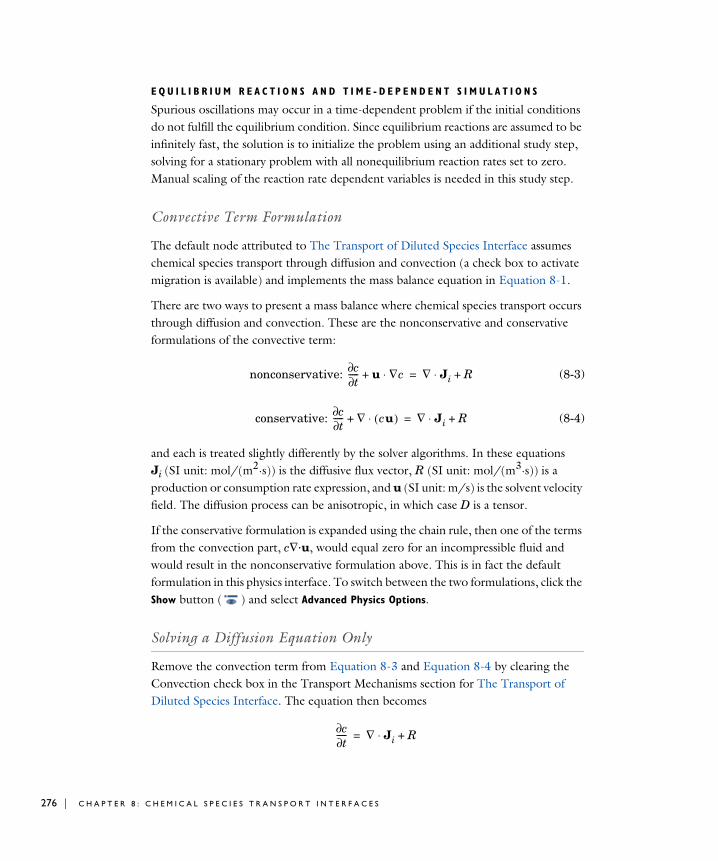
276 | C H A P T E

E Q U I L I B R I U M R E A C T I O N S A N D T I M E - D E P E N D E N T S I M U L A T I O N S

Spurious oscillations may occur in a time-dependent problem if the initial conditions do not fulfill the equilibrium condition. Since equilibrium reactions are assumed to be infinitely fast, the solution is to initialize the problem using an additional study step, solving for a stationary problem with all nonequilibrium reaction rates set to zero. Manual scaling of the reaction rate dependent variables is needed in this study step.

Convective Term Formulation

The default node attributed to The Transport of Diluted Species Interface assumes chemical species transport through diffusion and convection (a check box to activate migration is available) and implements the mass balance equation in Equation 8-1.

There are two ways to present a mass balance where chemical species transport occurs through diffusion and convection. These are the nonconservative and conservative formulations of the convective term:

nonconservative: (8-3)

conservative: (8-4)

and each is treated slightly differently by the solver algorithms. In these equations Ji (SI unit: mol/(m2·s)) is the diffusive flux vector, R (SI unit: mol/(m3·s)) is a production or consumption rate expression, and u (SI unit: m/s) is the solvent velocity field. The diffusion process can be anisotropic, in which case D is a tensor.

If the conservative formulation is expanded using the chain rule, then one of the terms from the convection part, c∇·u, would equal zero for an incompressible fluid and would result in the nonconservative formulation above. This is in fact the default formulation in this physics interface. To switch between the two formulations, click the Show button ( ) and select Advanced Physics Options.

Solving a Diffusion Equation Only

Remove the convection term from Equation 8-3 and Equation 8-4 by clearing the Convection check box in the Transport Mechanisms section for The Transport of Diluted Species Interface. The equation then becomes

c∂t∂----- u ∇c⋅+ ∇ Ji⋅ R+=

c∂t∂----- ∇ cu( )⋅+ ∇ Ji⋅ R+=

c∂t∂----- ∇ Ji⋅ R+=


Mass Sources for Species Transport

There are two types of mass sources in the Transport of Diluted Species interface: point sources and line sources.

Note: The features below are only available in a limited set of add-on products. For a detailed overview of which features are available in each product, visithttp://www.comsol.com/products/specifications/

P O I N T S O U R C E

A point source is theoretically formed by assuming a mass injection/ejection, (SI unit: mol/(m3·s)), in a small volume δV and then letting the size of the volume tend to zero while keeping the total mass flux constant. Given a point source strength, (SI unit: mol/s), this can be expressed as

(8-5)

An alternative way to form a point source is to assume that mass is injected/extracted through the surface of a small object. Letting the object surface area tend to zero while keeping the mass flux constant results in the same point source. For this alternative approach, effects resulting from the physical object’s volume need to be neglected.


is added at a point in the geometry. As can be seen from Equation 8-5, must tend to plus or minus infinity as δV tends to zero. This means that in theory the concentration also tends to plus or minus infinity.

Observe that “point” refers to the physical representation of the source. A point source can therefore only be added to points in 3D components and to points on the symmetry axis in 2D axisymmetry components. Other geometrical points in 2D components represent physical lines.

The finite element representation of Equation 8-5 corresponds to a finite concentration at a point with the effect of the point source spread out over a region around the point. The size of the region depends on the mesh and on the strength of

Q·

c

q·p,c

δV 0→lim Q

·c

δV q·p,c=

q·p,ctest c( )

Q·

c



278 | C H A P T E

the source. A finer mesh gives a smaller affected region but also a more extreme concentration value. It is important not to mesh too finely around a point source since this can result in unphysical concentration values. It can also have a negative effect on the condition number for the equation system.

L I N E S O U R C E

A line source can theoretically be formed by assuming a source of strength (SI unit: mol/(m3·s)), located within a tube with cross section δS and then letting δS tend to zero while keeping the total mass flux per unit length constant. Given a line source strength, (SI unit: mol/(m·s)), this can be expressed as

(8-6)

As in the point source case, an alternative approach is to assume that mass is injected/extracted through the surface of a small object. This results in the same mass source, but requires that effects resulting from the physical object’s volume are neglected.


is added on lines in 3D or at points in 2D (which represent cut-through views of lines). Line sources can also be added on the axisymmetry line in 2D axisymmetry components. It cannot, however, be added on geometrical lines in 2D since those represent physical planes.

As with a point source, it is important not to mesh too finely around the line source.

Q·

l,c

q· l,c

δS 0→lim Q· l,c

δS q· l,c=

q· l,ctest c( )

For feature node information, see Line Mass Source and Point Mass Source in the COMSOL Multiphysics Reference Manual.


Adding Transport Through Migration

Note: Migration is only available in a limited set of add-on products. For a detailed overview of which features are available in each product, visithttp://www.comsol.com/products/specifications/

In addition to transport due to convection and diffusion, the Transport of Diluted Species interface supports ionic species transport by migration. This is done by selecting the Migration in Electric Field check box under the Transport Mechanisms section for the physics interface. The mass balance then becomes:

(8-7)

where

• ci (SI unit: mol/ m3) denotes the concentration of species i

• Di (SI unit: m2/s) is the diffusion coefficient of species i

• u (SI unit: m/s) is the fluid velocity

• F (SI unit: A·s/mol) refers to Faraday’s constant

• V (SI unit: V) denotes the electric potential

• zi (dimensionless) is the charge number of the ionic species, and

• um,i (SI unit: mol·s/kg) is its ionic mobility

In this case the diffusive flux vector is

The velocity, u, can be a computed fluid velocity field from a Fluid Flow interface or a specified function of the spatial variables x, y, and z. The potential can be provided by an expression or by coupling the system of equations to a current balance, such as the Electrostatics interface. Sometimes it is assumed to be a supporting electrolyte present, which simplifies the transport equations. In that case, the modeled charged species concentration is very low compared to other ions dissolved in the solution. Thus, the species concentration does not influence the solution’s conductivity and the net charge within the fluid.

t∂∂ci ∇ Di∇ci– zium i, Fci V∇– ciu+( )⋅+ Ri=

Ji Di∇ci– zium i, Fci V∇–=



280 | C H A P T E

The Nernst-Einstein relation can in many cases be used for relating the species mobility to the species diffusivity according to

where R (SI unit: J/(mol·K)) is the molar gas constant and T (SI unit: K) is the temperature.

Note: In the Nernst-Planck Equations interface, the ionic species contribute to the charge transfer in the solution. It includes an electroneutrality condition and also computes the electric potential field in the electrolyte. For more information, see Theory for the Nernst-Planck Equations Interface. This interface is included in the Chemical Reaction Engineering Module.

Supporting Electrolytes

In electrolyte solutions, a salt can be added to provide a high electrolyte conductivity and decrease the ohmic losses in a cell. These solutions are often called supporting electrolytes, buffer solutions, or carrier electrolytes. The added species, a negative and a positive ion pair, predominates over all other species. Therefore, the supporting electrolyte species can be assumed to dominate the current transport in the solution. In addition, the predominant supporting ions are usually selected so that they do not react at the electrode surfaces since the high conductivity should be kept through the process, that is, they should not be electro-active species. This also means that the concentration gradients of the predominant species in a supporting electrolyte are usually negligible.

Modeling and solving for a supporting electrolyte in the Electrostatics or Secondary Current Distribution interfaces will give a potential distribution that drives the migration in the Transport of Diluted Species Interface.

The current density vector is proportional to the sum of all species fluxes as expressed by Faraday’s law:

um i,Di

RT--------=

i F ziNi

i=


The electroneutrality condition ensures that there is always a zero net charge at any position in a dilute solution. Intuitively, this means that it is impossible to create a current by manually pumping positive ions in one direction and negative ions in the other. Therefore, the convective term is canceled out to yield the following expression for the electrolyte current density, where j denotes the supporting species:

(8-8)

Equation 8-8 is simply Ohm’s law for ionic current transport and can be simplified to

(8-9)

where κ is the conductivity of the supporting electrolyte. A current balance gives the current and potential density in the cell

which, in combination with Equation 8-9, yields:

(8-10)

Equation 8-10 can be easily solved using the Electrostatics or Secondary Current Distribution interface and, when coupled to the Transport in Diluted Species interface, the potential distribution shows up in the migration term.

Crosswind Diffusion

Transport of diluted species applications can often result in models with a very high cell Péclèt number—that is, systems where convection or migration dominates over diffusion. Streamline diffusion and crosswind diffusion are of paramount importance to obtain physically reasonable results. The Transport of Diluted Species interface provides two crosswind diffusion options using different formulations. Observe that crosswind diffusion makes the equation system nonlinear even if the transport equation is linear.

D O C A R M O A N D G A L E Ã O

This is the formulation described in Numerical Stabilization in the COMSOL Multiphysics Reference Manual. The method reduces over- and undershoots to a minimum, even for anisotropic meshes.

i F zj2um j, F cj φ∇–

j=

i κ φ∇–=

∇ i⋅ 0=

∇ κ φ∇–( )⋅ 0=


282 | C H A P T E

In some cases, the resulting nonlinear equation system can be difficult to converge. This can happen when the cell Péclèt number is very high and the model contains many thin layers, such as contact discontinuities. You then have three options:

• Refine the mesh, especially in regions with thin layers.

• Use a nonlinear solver with a constant damping factor less than one.

• Switch to the Codina crosswind formulation.

C O D I N A

The Codina formulation is described in Ref. 1. It adds diffusion strictly in the direction orthogonal to the streamline direction. Compared to the do Carmo and Galeão formulation, the Codina formulation adds less diffusion but is not as efficient at reducing over- and undershoots. It also does not work as well for anisotropic meshes. The advantage is that the resulting nonlinear system is easier to converge and that underresolved gradients are less smeared out.

Danckwerts Inflow Boundary Condition

Constraining the composition to fixed values at an inlet to a reactor may sometimes result in issues with unreasonably high reaction rates or singularities at the inlet boundary. These problems may many times be mitigated by using a flux boundary condition instead, based on the inlet concentrations and the fluid velocity. In chemical engineering, this type of flux boundary condition is also known as a Danckwerts condition.

Use the Danckwerts condition to specify inlet concentrations to domains where high reaction rates are anticipated in the vicinity to the inlet (Ref. 2).

Given an inlet concentration ci,0, the Danckwerts inflow boundary condition reads

(8-11)

Mass Balance Equation for Transport of Diluted Species in Porous Media

V A R I A B L Y S A T U R A T E D P O R O U S M E D I A

The following equations for the molar concentrations, ci, describe the transport of solutes in a variably saturated porous medium for the most general case, when the pore space is primarily filled with liquid but also contain pockets or immobile gas:

n Ji uci+( )⋅ n uci 0,( )⋅=


(8-12)

On the left-hand side of Equation 8-12, the first three terms correspond to the accumulation of species within the liquid, solid, and gas phases, while the last term describes the convection due to the velocity field u (SI unit: m/s).

In Equation 8-12 ci denotes the concentration of species i in the liquid (SI unit: mol/m3), cP, i the amount adsorbed to solid particles (moles per unit dry weight of the solid), and cG, i the concentration of species i in the gas phase.

The equation balances the mass transport throughout the porous medium using the porosity εp, the liquid volume fraction θ; the matrix (drained) density, ρ = (1 − εp)ρp, and the solid phase density ρp.

For saturated porous media, the liquid volume fraction θ is equal to the porosity εp, but for partially saturated porous media, they are related by the saturation s as θ = sεp. The resulting gas volume fraction is av = εp − θ = (1-s)εp.

On the right-hand side of Equation 8-12, the first term introduces the spreading of species due to mechanical mixing resulting from the porous media (dispersion), as well as from diffusion and volatilization to the gas phase. The dispersion tensor is denoted DD (SI unit: m2/s) and the effective diffusion by De (SI unit: m2/s).

The last two terms on the right-hand side of Equation 8-12 describe production or consumption of the species; Ri is a reaction rate expression which can account for reactions in the liquid, solid, or gas phase, and Si is an arbitrary source term, for example due to a fluid flow source or sink.

Adsorption The time evolution of the adsorption, the solute transport to or from the solid phase, is defined by assuming that the amount of solute adsorbed to the solid, cP,i, is a function of the concentration in the fluid ci. This implies that the solute concentration in the liquid and solid phase are in instant equilibrium. The adsorption term can be expanded to give

(8-13)

where kP,i = ∂cP,i/∂ci is the adsorption isotherm.

t∂∂ θci( )

t∂∂ ρcP i,( )

t∂∂

+ avcG i,( ) u ∇ci⋅+ + =

∇ DD i, De i,+( ) ci∇[ ]⋅ R+ i S+i

t∂∂ ρcP i,( ) ρ

ci∂∂cP i,

t∂∂ci ρcP i, t∂

∂εP–= ρkP,i t∂∂ci ρcP i, t∂

∂εP–=


284 | C H A P T E

VolatilizationVolatilization is the process where a solute species in the liquid is transported to the gas phase due to vaporization. Assuming that the amount of solute in the gas phase, cG,i, is a linear function of the liquid phase concentration, the volatilization term is defined as

(8-14)

where kG,i = ∂cG,i/∂ci is the linear volatilization.

S A T U R A T E D P O R O U S M E D I A

In the case of transport in a saturated porous medium, θ = εp, and the governing equations are

(8-15)

Convection in Porous Media

Convection describes the movement of a species, such as a pollutant, with the bulk fluid velocity. The velocity field u corresponds to a superficial volume average over a unit volume of the porous medium, including both pores and matrix. This velocity is sometimes called Darcy velocity, and defined as volume flow rates per unit cross section of the medium. This definition makes the velocity field continuous across the boundaries between porous regions and regions with free flow.

The average linear fluid velocities ua, provides an estimate of the fluid velocity within the pores:

t∂∂ avcG i, av ci∂

∂cG i,t∂

∂ci kG i, ci t∂∂av+= avkG i, t∂

∂ci kG i, ci t∂∂av+=

t∂∂ εpci( )

t∂∂ ρcP i,( ) u ∇ci⋅+ + ∇ DD i, De i,+( ) ci∇[ ]⋅ R+ i S+

i=

The velocity field to be used in the Model Inputs section on the physics interface can, for example, be prescribed using the velocity field from a Darcy’s Law or a Brinkman Equations interface.

uauεp-----= Saturated

uauθ----= Partially saturated


where εp is the porosity and θ = sεp the liquid volume fraction, and s the saturation, a dimensionless number between 0 and 1.

Figure 8-1: A block of a porous medium consisting of solids and the pore space between the solid grains. The average linear velocity describes how fast the fluid moves within the pores. The Darcy velocity attributes this flow over the entire fluid-solid face.

C O N V E C T I V E T E R M F O R M U L A T I O N

The Transport of Diluted Species in Porous Media interface includes two formulations of the convective term. The conservative formulation of the species equations in Equation 8-12 is written as:

(8-16)

If the conservative formulation is expanded using the chain rule, then one of the terms from the convection part, ci∇·u, would equal zero for an incompressible fluid and would result in the nonconservative formulation described in Equation 8-12.

When using the nonconservative formulation, which is the default, the fluid is assumed incompressible and divergence free: ∇ ⋅ u = 0. The nonconservative formulation

t∂∂ θci( )

t∂∂ ρbcP i,( )

t∂∂

+ avcG i,( ) ∇ uci⋅+ + =

∇ DD i, De i,+( ) ci∇[ ]⋅ R+ i S+i


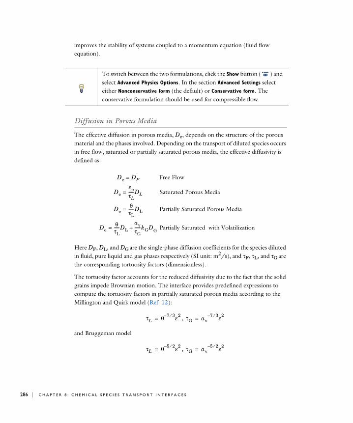
286 | C H A P T E

improves the stability of systems coupled to a momentum equation (fluid flow equation).

Diffusion in Porous Media

The effective diffusion in porous media, De, depends on the structure of the porous material and the phases involved. Depending on the transport of diluted species occurs in free flow, saturated or partially saturated porous media, the effective diffusivity is defined as:

Here DF, DL, and DG are the single-phase diffusion coefficients for the species diluted in fluid, pure liquid and gas phases respectively (SI unit: m2/s), and τF, τL, and τG are the corresponding tortuosity factors (dimensionless).

The tortuosity factor accounts for the reduced diffusivity due to the fact that the solid grains impede Brownian motion. The interface provides predefined expressions to compute the tortuosity factors in partially saturated porous media according to the Millington and Quirk model (Ref. 12):

,

and Bruggeman model

,

To switch between the two formulations, click the Show button ( ) and select Advanced Physics Options. In the section Advanced Settings select either Nonconservative form (the default) or Conservative form. The conservative formulation should be used for compressible flow.

De DF= Free Flow

DeεpτL-----DL= Saturated Porous Media

DeθτL-----DL= Partially Saturated Porous Media

DeθτL-----DL

avτG------kGDG+= Partially Saturated with Volatilization

τL θ 7– 3⁄ ε2= τG av

7– 3⁄ ε2=

τL θ 5– 2⁄ ε2= τG av

5– 2⁄ ε2=


For saturated porous media θ = εp. The fluid tortuosity for the Millington and Quirk model is

and for the Bruggeman model the tortuosity is defined as

User defined expressions for the tortuosity factor can also be applied.

Dispersion

The contribution of dispersion to the mixing of species typically overshadows the contribution from molecular diffusion, except when the fluid velocity is very small.

The spreading of mass, as species travel through a porous medium is caused by several contributing effects. Local variations in fluid velocity lead to mechanical mixing referred to as dispersion occurs because the fluid in the pore space flows around solid particles, so the velocity field varies within pore channels. The spreading in the direction parallel to the flow, or longitudinal dispersivity, typically exceeds the transverse dispersivity from up to an order of magnitude. Being driven by the concentration gradient alone, molecular diffusion is small relative to the mechanical dispersion, except at very low fluid velocities.

Figure 8-2: Spreading of fluid around solid particles in a porous medium.

is controlled through the dispersion tensor DD. The tensor components can either be given by user-defined values or expressions, or derived from the directional dispersivities.

Using the longitudinal and transverse dispersivities in 2D, the dispersivity tensor components are (Ref. 9):

τL εp1– 3⁄

=

τL εp1– 2⁄

=


288 | C H A P T E

In these equations, DDii (SI unit: m2/s) are the principal components of the dispersivity tensor, and DDji and DDji are the cross terms. The parameters αL and αT (SI unit: m) specify the longitudinal and transverse dispersivities; and ui (SI unit: m/s) stands for the velocity field components.

In order to facilitate modeling of stratified porous media in 3D, the tensor formulation by Burnett and Frind (Ref. 10) can be used. Consider a transverse isotropic media, where the strata are piled up in the z direction, the dispersivity tensor components are:

(8-17)

In Equation 8-17 the fluid velocities u, v, and w correspond to the components of the velocity field u in the x, y, and z directions, respectively, and α1 (SI unit: m) is the longitudinal dispersivity. If z is the vertical axis, α2 and α3 are the dispersivities in the transverse horizontal and transverse vertical directions, respectively (SI unit: m). Setting α2 = α3 gives the expressions for isotropic media shown in Bear (Ref. 9 and Ref. 11).

Adsorption

As species travel through a porous medium they typically attach to (adsorb), and detach (desorb) from the solid phase, which slows chemical transport through the porous medium. Adsorption and desorption respectively reduces or increases species

DDii αLui

2

u------- αT

uj2

u-------+=

DDij DDji αL αT–( )uiuj

u-----------= =

DLxx α1u2

u------- α2

v2

u------- α3

w2

u-------+ +=

DLyy α1v2

u------- α2

u2

u------- α3

w2

u-------+ +=

DLzz α1w2

u------- α3

u2

u------- α3

v2

u-------+ +=

DLxy DLyx α1 α2–( )uvu-------= =

DLxz DLzx α1 α3–( )uwu--------= =

DLyz DLzy α1 α3–( )vwu--------= =


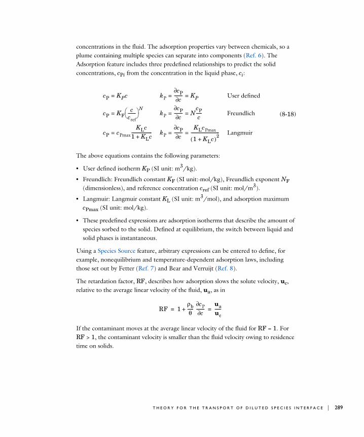
concentrations in the fluid. The adsorption properties vary between chemicals, so a plume containing multiple species can separate into components (Ref. 6). The Adsorption feature includes three predefined relationships to predict the solid concentrations, cPi from the concentration in the liquid phase, ci:

(8-18)

The above equations contains the following parameters:

• User defined isotherm KP (SI unit: m3/kg).

• Freundlich: Freundlich constant KF (SI unit:·mol/kg), Freundlich exponent NF (dimensionless), and reference concentration cref (SI unit: mol/m3).

• Langmuir: Langmuir constant KL (SI unit: m3/mol), and adsorption maximum cPmax (SI unit: mol/kg).

• These predefined expressions are adsorption isotherms that describe the amount of species sorbed to the solid. Defined at equilibrium, the switch between liquid and solid phases is instantaneous.

Using a Species Source feature, arbitrary expressions can be entered to define, for example, nonequilibrium and temperature-dependent adsorption laws, including those set out by Fetter (Ref. 7) and Bear and Verruijt (Ref. 8).

The retardation factor, RF, describes how adsorption slows the solute velocity, uc, relative to the average linear velocity of the fluid, ua, as in

If the contaminant moves at the average linear velocity of the fluid for RF = 1. For RF > 1, the contaminant velocity is smaller than the fluid velocity owing to residence time on solids.

cP KPc= kPcP∂c∂-------- KP= = User defined

cP KFc

cref-------- N

= kPcP∂c∂-------- N

cPc------= = Freundlich

cP cPmaxKLc

1 KLc+--------------------= kP

cP∂c∂--------

KLcPmax

1 KLc+( )2----------------------------= = Langmuir

RF 1ρbθ------

cP∂c∂--------+

uauc------= =


290 | C H A P T E

Reactions

Chemical reactions of all types influence species transport in porous media. Examples include biodegradation, radioactive decay, transformation to tracked products, temperature- and pressure-dependent functions, exothermic reactions, and endothermic reactions. The reactions represent change in species concentration per unit volume porous medium per time. Reaction terms are used on the right-hand side of the governing equation to represent these processes. For reactions in a fluid phase, multiply the expression by the fluid volume fraction θ. Similarly, solid phase reaction expressions include the bulk density, ρb, and gas phase reactions include the gas volume fraction, av.

References

1. R. Codina, “A discontinuity-capturing crosswind-dissipation for the finite element solution of the convection-diffusion equation”, Computer Methods in Applied Mechanics and Engineering, vol. 110, pp. 325–342, 1993.

2. P.V. Danckwerts, “Continuous flow systems: Distribution of residence times”, Chem. Eng. Sci., vol. 2, no. 1, 1953.

3. J.M. Coulson and J.F. Richardson, Chemical Engineering, vol. 2, 4th ed., Pergamon Press, Oxford, U.K., 1991.

4. J.M. Coulson and J.F. Richardson, Chemical Engineering, vol. 1, 4th ed., Pergamon Press, Oxford, U.K., 1991.

5. D.E Rosner, Transport Processes in Chemically Reacting Flow Systems, ISBN-13: 978-1483130262, Butterworth-Heinemann, 1986

6. D.M. Mackay, D.L. Freyberg, P.V. Roberts, and J.A. Cherry, “A Natural Gradient Experiment on Solute Transport in a Sand Aquifer: 1. Approach and Overview of Plume Movement”, Water Resourc. Res., vol. 22, no. 13, pp. 2017–2030, 1986.

7. C.W. Fetter, Contaminant Hydrogeology, Prentice Hall, 1999.

8. J. Bear and A. Verruijt, Modeling Groundwater Flow and Pollution, D. Reidel Publishing, 1994.

9. J. Bear, Hydraulics of Groundwater, McGraw-Hill, 1979.

10. R.D. Burnett and E.O. Frind, “An Alternating Direction Galerkin Technique for Simulation of Groundwater Contaminant Transport in Three Dimensions: 2. Dimensionality Effects”, Water Resour. Res., vol. 23, no. 4, pp. 695–705, 1987.


11. J. Bear, Dynamics of Fluids in Porous Media, Elsevier Scientific Publishing, 1972.

12. R.J. Millington and J.M. Quirk, “Permeability of Porous Solids”, Trans. Faraday Soc., vol. 57, pp. 1200–1207, 1961.

13. I. Langmuir, “Chemical Reactions at Low Temperatures”, J. Amer. Chem. Soc., vol. 37, 1915.

14. R.B. Bird, W.E. Stewart, and E.N. Lightfoot, Transport Phenomena, 2nd ed., John Wiley & Sons, Inc., 2007.


292 | C H A P T E

9

G l o s s a r y

This Glossary of Terms contains finite element modeling terms specific to the Microfluidics Module and its applications. For mathematical terms as well as geometry and CAD terms specific to the COMSOL Multiphysics® software and its documentation, see the glossary in the COMSOL Multiphysics Reference Manual. To find references in the documentation set where you can find more information about a given term, see the index.

293

294 | C H A P T E

G l o s s a r y o f T e rm sabsorption (gas) Uptake of a gas into the bulk of a liquid. Gas absorption takes place, for example, in the liquid of a scrubber tower where an up-streaming gas is washed by a down-going flow of a scrubber solution.

adsorption (molecule) Attachment of a molecule or atom to a solid surface. Adsorption involves a chemical bond between the adsorbed species and the surface.

ALE See arbitrary Lagrangian-Eulerian method.

arbitrary Lagrangian-Eulerian (ALE) method A technique to formulate equations in a mixed kinematical description. An ALE referential coordinate system is typically a mix between the material (Lagrangian) and spatial (Eulerian) coordinate systems.

biosensor A general term for sensor devices that either detect biological substances or use antibodies, enzymes, or other biological molecules in their operation. Biosensors are a subcategory of chemical sensors.

Bond number A dimensionless number given by the ratio of surface tension forces to body forces (usually gravity) for a two-phase flow. It is also known as the Eötvös number, Eo. At high Bond numbers surface tension has a minimal effect on the flow; at low Bond numbers, surface tension dominates. The Bond number, Bo, is given by:

where ρ is the density, g is the body force acceleration, L is the characteristic length, and σ is the surface tension coefficient. The density can refer to a density difference when considering buoyancy.

Brinkman equations A set of equations extending Darcy’s law in order to include the transport of momentum through shear in porous media flow.

capillary number A dimensionless number given by the ratio of viscous forces to surface tension for a two phase flow. At low capillary numbers flow in porous media is dominated by surface tension. The capillary number, Ca, is given by:

Bo ρgL2

σ--------------=

R 9 : G L O S S A R Y

where μ is the viscosity, v is the characteristic velocity of the problem, and σ is the surface tension coefficient.

continuum flow Fluid flow which is well described by approximating the liquid as a continuum with the Navier-Stokes equations.

convection Transport of molecules or heat due to the movement of the surrounding medium.

creeping flow Models the Navier-Stokes equations without the contribution of the inertia term. This is often referred to as Stokes flow and is appropriate for use when viscous flow is dominant, such as in very small channels or microfluidic applications.

crosswind diffusion A numerical technique for stabilization of the numeric solution to a convection-dominated PDE by artificially adding diffusion perpendicular to the direction of the streamlines.

Darcy’s Law Equation that gives the velocity vector as proportional to the pressure gradient. Often used to describe flow in porous media.

Debye layer See electric double layer.

dielectrophoresis (DEP) Migration of polarizable particles in an electrolyte in a nonuniform applied electric field.

diffusion Transport of material resulting from the random motion of molecules in the presence of a concentration gradient.

Dukhin number A dimensionless number given by the ratio of the surface conductivity contribution to the fluid bulk electrical conductivity contribution in electrokinetic phenomena. The Dukhin number, Du, is given by:

where Kσ is the surface conductivity and KB is the bulk conductivity. For low Dukhin numbers, surface conductivities can be neglected when modeling electrokinetic flows.

Ca μvσ------=

Du Kσ

KB--------=

G L O S S A R Y O F T E R M S | 295

296 | C H A P T E

electric double layer (EDL) Sometimes referred to as the Debye layer. At the contact of a solid and a polar fluid (such as water), the solid acquires an electric charge. This charge attracts ions within the fluid, and a narrow fluid layer of opposite charge, the Stern layer, forms on the boundary. In addition, adjacent to the Stern layer, a wider layer with the same charge as in the Stern layer forms in the fluid. Together, the Stern layer and the wider layer (called the diffuse or Gouy-Chapman layer) form the electric double layer. Due to the close distance between the charges, the Stern layer is fixed on the surface, but the more distant diffuse layer can move.

electrohydrodynamics A general term describing phenomena that involve the interaction between solid surfaces, ionic solutions, and applied electric and magnetic fields. It is frequently used in microfluidic devices to manipulate fluids and move particles for sample handling and chemical separation.

electrokinetics Study of the motion of charged particles under an applied electric field in moving substances such as water.

electrokinetic flow Transport of fluid or charged particles within a fluid by means of electric fields. See also electroosmosis, electrophoresis, electrothermal flow, and dielectrophoresis.

electrolyte A solution that can carry an electric current through the motion of ions.

electroosmosis Fluid flow in a narrow channel produced by the movement of the electric double layer (EDL) along the channel boundary under the influence of an applied electric field. Also, fluid flow through a membrane under the influence of an applied electric field. See also electric double layer.

electroosmotic flow See electroosmosis.

electrophoresis Migration of charged electrolyte ions or particles in an applied electric field.

electrothermal effects These effects occur in a conductive fluid where the temperature is modified by Joule heating from an AC electric field. This creates variations in conductivity and permittivity and thus Coulomb and dielectric body forces.


electrothermal flow Fluid flow resulting from an applied nonuniform AC electric field on a fluid. The Joule heating changes the fluid’s electrical properties locally, and that effect, together with the power gradient of the AC electric field, results in fluid motion.

electrowetting The electrowetting effect describes the change in solid-electrolyte contact angle that occurs when a potential difference is applied between the solid and the electrolyte.

electrowetting-on-dielectric (EWOD) A form of electrowetting in which a thin insulating layer separates the conducting solid surface from the electrolyte.

Eötvös number See Bond number.

Eulerian frame A frame of reference with its coordinate axes fixed in space.

Fick’s laws The first law relates the concentration gradients to the diffusive flux of low concentration solute diluted in a solvent. The second law introduces the first law into a differential material balance for the solute.

fluid-structure interaction (FSI) When a flow affects the deformation of a solid object and vice versa.

free molecular flow The flow of gas molecules through a geometry which is much smaller than the mean free path (Knudsen number, Kn>10). In the free molecular flow regime the gas molecules collide with the walls of the geometry much more frequently than they collide with themselves.

fully developed laminar flow Laminar flow along a channel or pipe that has velocity components only in the main direction of the flow. The velocity profile perpendicular to the flow does not change downstream in the flow.

Gouy-Chapman layer See electric double layer (EDL).

Hagen-Poiseuille equation See Poiseuille’s law.

Helmholtz-Smoluchowski equation Gives the velocity of a parallel electroosmotic flow for an applied electric field.

intrinsic volume averages The physical properties of the fluid, such as density, viscosity, and pressure.


298 | C H A P T E

Knudsen number A dimensionless number that provides a measure of how rarefied a gas flow is, in other words, the mean free path of the gas molecules compared to the length scale of the flow. The following equation defines the Knudsen number Kn where λ is the mean free path of the molecules and L is a length scale characteristic to the flow.

Knudsen layer A layer of rarefied fluid flow that occurs within a few mean free paths of the walls in a gas flow. The continuum Navier-Stokes equations break down in this layer.

Lagrangian frame A frame of reference with its coordinate axes fixed in a reference configuration of a deforming material. As the material deforms, the Lagrangian frame deforms with it.

Laplace number The Laplace number, La, (also known as the Surataman number, Su) relates the inertial and surface tension forces to the viscous forces. It is used to describe the breakup of liquid jets and sheets: at high Laplace and low Reynolds numbers the Rayleigh Instability occurs, at low Laplace and high Reynolds numbers atomization occurs. The Laplace number is given by:

where ρ is the fluid density, σ is the surface tension coefficient, L is the characteristic length scale of the problem, and μ is the viscosity. The Laplace number is directly related to the Ohnesorge number, Oh, through the equation La=1/Oh2.

Mach number Ratio of the convective speed, v, to the speed of sound in the medium, a. The Mach number, Ma, is defined by the equation:

magnetohydrodynamics Fluid-flow phenomena involving magnetic fields.

magnetophoresis Migration of magnetic or paramagnetic particles suspended in a fluid as a result of an applied magnetic field. The field must be nonuniform in the case of paramagnetic particles.

Kn λL----=

La ρσL

μ2-----------=

Ma va---=


Marangoni effect Fluid flow parallel to an interface induced by surface tension gradients.

Marangoni number Ratio of thermal surface tension forces to viscous forces. The Marangoni number, Mg, is given by:

where σ is the surface tension coefficient, T is the absolute temperature (ΔT is the characteristic temperature difference), L is the characteristic length, and α is the thermal diffusivity (α=κ/(ρcp)), where cp is the heat capacity at constant pressure, κ is the thermal conductivity, and ρ is the density of the fluid.

microfluidics Study of the behavior of fluids at the microscale. Also refers to MEMS fluidic devices.

migration The transport of charged species in an electrolyte due to the electric force imposed by the electric field.

mobility The relation between the drift velocity of a molecule within a fluid and the applied electric field.

Newtonian flow Flow characterized by a constant viscosity or a viscosity that is independent of the shear rate in the fluid.

Nernst-Planck equation Flow equation that describes the flux of an ion through diffusion, convection, and migration in an electric field. The equation is valid for diluted electrolytes.

Ohnesorge number A dimensionless number relating the inertial and surface tension forces to the viscous forces. Used to describe the breakup of liquid jets and sheets: at low Ohnesorge and Reynolds numbers the Rayleigh instability occurs; at high Ohnesorge and Reynolds numbers, atomization occurs. The Ohnesorge number, Oh, is given by:

Mg dσdT--------LΔT

μα------------=

Oh μρσL---------------=


300 | C H A P T E

where ρ is the fluid density, σ is the surface tension coefficient, L is the characteristic length scale of the problem, and μ is the viscosity. The Ohnesorge number is directly related to the Laplace number, La, through the equation Oh=1/La1/2.

Peclet number A dimensionless number describing the ratio of convection to diffusion in a fluid flow. The Peclet number, Pe, can be used to describe concentration diffusion or heat diffusion. It is given by:

where v is the convective velocity, L is the flow length scale, and D is the diffusion constant.

Poiseuille’s law Equation that relates the mass rate of flow in a tube as proportional to the pressure difference per unit length and to the fourth power of the tube radius. The law is valid for fully developed laminar flow.

Reynolds number A dimensionless number classifying how laminar or turbulent a flow is. The Reynolds number Re is a measure of the relative magnitude of the flow’s viscous and inertial forces. It is defined by the following equation where ρ is the fluid density, μ is the dynamic viscosity, ν is its kinematic viscosity, v is a velocity characteristic to the flow, and L is a length scale characteristic to the flow.

slip flow Fluid flow that occurs when the Knudsen number, Kn, is in the range 0.01<Kn<0.1. As a result of rarefaction effects in the Knudsen layer the no slip boundary condition fails. The flow outside the Knudsen layer can be represented by the continuum Navier-Stokes equations provided that an appropriate slip boundary condition is used for the fluid flow and the correct temperature jump boundary condition is applied at the interface.

streamline diffusion A numerical technique for stabilization of the numeric solution to a convection-dominated PDE by artificially adding diffusion in the direction of the streamlines.

Stern layer A layer of immobile ions and associated solvent molecules present at the solid-liquid interface in an electric double layer (EDL).

Pe vLD-------=

Re ρvLμ----------- vL

ν-------= =


Stokes flow See creeping flow.

superficial volume averages The flow velocities, which correspond to a unit volume of the medium including both pores and matrix. They are sometimes called Darcy velocities, defined as volume flow rates per unit cross section of the medium.

surface tension Surface tension is a property of the surface of a liquid that allows it to resist an external force. Equivalently it can be through of as the energy per unit area of the liquid surface. It is caused by asymmetries in the cohesive forces between molecules at the surface of the liquid.

Surataman number See Laplace number.

transitional flow Fluid flow that occurs when the Knudsen number, Kn, is in the range 0.1<Kn<10. In this regime the flow is so rarefied that continuum equations break down completely. However collisions between the molecules are still important, so free molecular flow is not applicable.

Weber number A dimensionless number describing the ratio of inertial forces to surface tension forces. The Weber number is given by:

where ρ is the density of the fluid, v is the characteristic velocity of the flow, L is the characteristic length scale, and σ is the surface tension coefficient.

zeta potential The potential of at the interface between the electric double layer and a solid surface in an electrolyte.

We ρv2Lσ

-------------=


302 | C H A P T E

I n d e x

A absolute pressure 67, 120, 126, 131, 209

AC electric fields 52

AC electroosmosis 48

AC/DC Module 51

adsorption 261

Application Libraries window 23

application library examples

convection and diffusion 245

creeping flow 61

electroosmosis 49

electrowetting lens 53

laminar flow 65

laminar, two-phase flow, moving mesh

135

level set conservation 181

migration in electric field 245

slip flow 226

transport of diluted species 240

B Bond and Eötvös numbers 34

boundary nodes

Brinkman equations 205

Darcy’s law interface 195

free and porous media flow 211

level set 163

phase field 168

slip flow 226

ternary phase field 174


boundary stress (node) 78


Brinkman equations interface 203

theory 219

C Cahn-Hilliard equation 184, 189

capillary number 34

CFL number

settings 65, 205

chemical potential variable 188

Chemical Reaction Engineering Module

15, 44

chemical transport and reactions, mode-

ling 44

Clausius-Mosotti factor

dielectrophoresis 50

magnetophoresis 51

common settings 20

complex permittivity 50

concentration (node)


continuity (node) 230

continuity equation, Darcy’s law 217

continuum flow 56

convection 284

convective terms, diluted species 276

coupling interfaces 46

coupling, fluid flow and electric fields 46

creeping flow 135, 224

creeping flow (spf) interface 60

crosswind diffusion, in fluid flow 32

D Darcy velocity 200, 217, 284


theory 217

Debye layer, electroosmosis and 47

Debye length 48

Debye-Hückel approximation 47

dielectrophoresis (DEP) 50

dimensionless numbers 31–33

Dirichlet boundary condition 32

documentation 21

domain nodes


Darcy’s law 195

I N D E X | 303

304 | I N D E X


level set 163

phase field 168

slip flow 226



Dukhin number 34

E edge nodes


slip flow 226

electric double layer (EDL), electroos-

mosis and 47

electrode-electrolyte interface coupling

(node)


electrohydrodynamics, definition 46

electrokinetic flows 46

electrokinetics 46

electroosmosis 47

electroosmotic velocity, wall boundary

condition 70

electrophoresis 46, 49

electrothermally driven flow 52

electrowetting on dielectric (EWOD) 53

emailing COMSOL 23

Equilibrium Reaction

theory for 274

equilibrium reaction (node) 255

external fluid interface (node) 137

external slip wall (node) 228

F Faraday’s law 280

flow continuity (node) 81

flow rate in SCCMs 74

flow regimes, for rarefied flows 56

fluid (node) 227

fluid and matrix properties (node)


Darcy’s law 197

fluid flow

Brinkman equations theory 219

Darcy’s law theory 217

electrothermally driven 52

two-phase flow moving mesh theory

152

fluid properties (node)


single-phase, laminar flow 66

fluid-fluid interface (node) 136

flux (node)


flux discontinuity (node) 250

Darcy’s law 200


Forchheimer drag (node)



free and porous matrix properties

(node) 213

free and porous media flow interface 210

theory 222

Freundlich exponent 289

fully developed flow 75

G general stress (boundary stress condi-

tion) 79

geometry frames 153

Ginzburg-Landau equation 185

gravity 83

H heat transfer 54

Heat Transfer Module 54

Helmholtz-Smoluchowski equation 48

Henry’s function 49

Hygroscopic Swelling 270

I inflow (node) 248

initial interface (node)

level set 166

phase field 171

initial values (node)


Darcy’s law 198


level set 164, 170

phase field 176

single-phase, laminar flow 69

slip flow 229


initializing functions 182, 187

inlet (node) 199

single-phase flow 72

ternary phase field 176–177

interface normal variable 183

interior wetted wall (node) 172

internet resources 21

intrinsic volume averages 219

isotropic diffusion 32

J Joule heating 52

K knowledge base, COMSOL 24

Knudsen layer 57

Knudsen number 14, 34, 56

L lab-on-a-chip devices 14

laminar flow interface 61

laminar three-phase flow, phase field in-

terface 129

laminar two-phase flow

moving mesh interface 134

laminar two-phase flow, level set (tpf) in-

terface 118, 124

Langmuir constant 289

Laplace number 35

leaking wall, wall boundary condition 71,

216

level set functions, initializing 182, 187

level set interface 162

theory 141, 179

level set model (node) 164

line mass source (node)

fluid flow 82

species transport 252

line source


local

CFL number 65, 205

M Mach number 34

magnetohydrodynamics 46

magnetophoresis 46, 51

Marangoni number 35

mass based concentrations (node) 246

mass conservation, level set equations

144

mass flux (node) 199

mass source (node)


Darcy’s law 198

material frames 153

mathematics, moving interfaces

level set 162

phase field 167, 173

theory 179, 184, 189

MEMS Module 215

MEMS, definition 14

mesh frames 153

microfluidic wall conditions (node) 214

microfluidics

definition 14

dimensionless numbers, and 31–33

modeling techniques 28

stabilization techniques 32

mixture properties (node) 174

modeling

electrohydrodynamics 46

microfluidics 28

I N D E X | 305

306 | I N D E X

transport of chemical species and ions

44

moving interfaces 184, 189

MPH-files 23

multiphase flow

moving mesh theory 152

multiphase flow theory 141, 179, 184, 189

N Navier-Stokes equations 141

Nernst-Einstein relation 244, 260, 264,

280

no flow (node)

Darcy’s law 200

level set 166

no flux (node) 248

no slip, wall boundary condition 70, 216

no viscous stress (open boundary) 78

nodes, common settings 20

non-conservative formulations 144

nonconservative formulations 276

normal stress, normal flow (boundary

stress condition) 79

numerical instability, dimensionless num-

bers and 31

O Ohm’s law 281

Ohnesorge number 35

open boundary (node)



outflow (node)


outlet (node) 201



P pair nodes




level set 163

phase field 168

slip flow 226



partially saturated porous media (node)

262

Peclet number 31

periodic condition (node) 230


periodic flow condition (node) 80

permeability models 198

phase field interface 167

theory 141, 184, 189

phase field model (node) 169

physics interfaces, common settings 20

point mass source (node)

fluid flow 82


point nodes




slip flow 226

point source


porous electrode coupling (node) 257

porous media and subsurface flow

Brinkman equations interface 203


free and porous media flow interface

210

theory, Brinkman equations 219

theory, Darcy’s law 217

theory, free and porous media flow

222

porous media transport properties

(node) 259

pressure (node) 198

pressure point constraint (node) 81

pseudo time stepping

settings 65, 205

R rarefied gas flow 56

Reacting Volume 247

reaction coefficients (node) 258

Reactions

in porous catalyst pellets 268

reactions (node)


reactive pellet bed (node) 265

retardation factor 289

Reynolds number, dimensionless num-

bers and 31

S SCCM, flow rate in 74

selecting

multiphase flow interfaces 39

porous media flow interfaces 40

single-phase flow interfaces 37

SEMI standard E12-0303 74

shear rate magnitude variable 68

single-phase flow interface

laminar flow 61

sliding wall 72

slip

Maxwell’s boundary condition 57

slip flow 57

slip flow interface 224

theory 231

slip velocity, wall boundary condition 70

slip wall (node) 229

slip, wall boundary condition 70, 216

spatial frames 153

spf.sr variable 68

stabilization techniques, dimensionless

numbers and 32

standard cubic centimeters per minute

74

standard flow rate 74

standard settings 20

Stern layer 48

Stokes equations 60

Stokes flow 60, 135

stratified porous media 288

streamline diffusion, in fluid flow 32

superficial volume average, porous me-

dia 220

superficial volume averages, porous me-

dia 284

Supporting Electrolytes 280

Surataman number 35

surface equilibrium reaction (node) 256

surface tension force variable 188

symmetry (node) 77, 230

Darcy’s law 200


T technical support, COMSOL 23

ternary phase field interface 173

theory


Darcy’s law 217


level set 179

phase field 184, 189

slip flow 231

tpf interfaces 141

transport of diluted species in porous

media interface 273

transport of diluted species interface

272

two-phase flow moving mesh 152

thermal creep, wall boundary condition

71

thickness

fracture 270

I N D E X | 307

308 | I N D E X

out-of-plane 202

thin barrier (node)

level set 166

thin diffusion barrier (node) 254

Thin Impermeable Barrier 254

TMAC, microfluidic wall conditions 215

tortuosity factors 286

traction boundary conditions 78

transport of diluted species in porous

media interface 240

theory 273

transport of diluted species interface 236

theory 272

turbulent mixing (node)


two-phase flow

moving mesh, theory 152

V variables

level set interface 183

phase field interface 188

viscous slip, wall boundary condition 70

volume averages 219

volume force (node) 69



W wall (node)



wall fluid interface (node) 139

Weber number 35

websites, COMSOL 24

wetted wall (boundary condition) 122

wetted wall (node) 171, 177

Y Young’s equation 52

the microfluidics module user’s guide

Documents